NBER WORKING PAPER SERIES

PREDICTING THE EQUITY PREMIUM OUT OF SAMPLE:CAN ANYTHING BEAT THE HISTORICAL AVERAGE?

John Y. CampbellSamuel B. Thompson

Working Paper 11468http://www.nber.org/papers/w11468

NATIONAL BUREAU OF ECONOMIC RESEARCH1050 Massachusetts Avenue

Cambridge, MA 02138June 2005

Both authors: Department of Economics, Littauer Center, Harvard University, Cambridge MA 02138, USA,and NBER. Email john_campbell@harvard.edu and sthompson@harvard.edu. We are grateful to Jan Szilagyifor able research assistance, to Amit Goyal and Ivo Welch for sharing their data, and to Malcolm Baker, LutzKilian, Martin Lettau, Sydney Ludvigson, and Rossen Valkanov for helpful comments on an earlier draft.This material is based upon work supported by the National Science Foundation under Grant No. 0214061to Campbell. The views expressed herein are those of the author(s) and do not necessarily reflect the viewsof the National Bureau of Economic Research.

©2005 by John Y. Campbell and Samuel B. Thompson. All rights reserved. Short sections of text, not toexceed two paragraphs, may be quoted without explicit permission provided that full credit, including ©notice, is given to the source.

Predicting the Equity Premium Out Of Sample: Can Anything Beat the Historical Average?John Y. Campbell and Samuel B. ThompsonNBER Working Paper No. 11468June 2005JEL No. G1

ABSTRACT

A number of variables are correlated with subsequent returns on the aggregate US stock market in

the 20th Century. Some of these variables are stock market valuation ratios, others reflect patterns

in corporate finance or the levels of shortand long-term interest rates. Amit Goyal and Ivo Welch

(2004) have argued that in-sample correlations conceal a systematic failure of these variables out of

sample: None are able to beat a simple forecast based on the historical average stock return. In this

note we show that forecasting variables with significant forecasting power insample generally have

a better out-of-sample performance than a forecast based on the historical average return, once

sensible restrictions are imposed on the signs of coefficients and return forecasts. The out-of-sample

predictive power is small, but we find that it is economically meaningful. We also show that a

variable is quite likely to have poor out-of-sample performance for an extended period of time even

when the variable genuinely predicts returns with a stable coefficient.

John Y. CampbellDepartment of EconomicsHarvard UniversityLittauer Center 213Cambridge, MA 02138and NBERjohn_campbell@harvard.edu

Samuel B. ThompsonDepartment of EconomicsHarvard UniversityLittauer Center 125Cambridge, MA 02138sthompson@harvard.edu

1 Introduction

Towards the end of the last century, academic finance economists came to take se-riously the view that aggregate stock returns are predictable. During the 1980’s anumber of papers studied valuation ratios, such as the dividend-price ratio, earnings-price ratio, or smoothed earnings-price ratio. Value-oriented investors in the traditionof Graham and Dodd (1934) had always asserted that high valuation ratios are an in-dication of an undervalued stock market and should predict high subsequent returns,but these ideas did not carry much weight in the academic literature until authorssuch as Rozeff (1984), Fama and French (1988), and Campbell and Shiller (1988a,b)found that valuation ratios are positively correlated with subsequent returns and thatthe implied predictability of returns is substantial at longer horizons. Around thesame time, several papers pointed out that yields on short- and long-term Treasuryand corporate bonds are correlated with subsequent stock returns (Fama and Schwert1977, Keim and Stambaugh 1986, Campbell 1987, Fama and French 1989).

During the 1990’s and early 2000’s, research continued on the prediction of stockreturns from valuation ratios (Kothari and Shanken 1997, Pontiff and Schall 1998) andinterest rates (Hodrick 1992). Several papers suggested new predictor variables ex-ploiting information in corporate payout and financing activity (Lamont 1998, BakerandWurgler 2000), the level of consumption in relation to wealth (Lettau and Ludvig-son 2001), and the relative valuations of high- and low-beta stocks (Polk, Thompson,and Vuolteenaho 2003). At the same time, several authors expressed concern thatthe apparent predictability of stock returns might be spurious. Many of the predictorvariables in the literature are highly persistent, and Stambaugh (1999) pointed outthat persistence leads to biased coefficients in predictive regressions if innovations inthe predictor variable are correlated with returns (as is strongly the case for valuationratios, although not for interest rates). Under the same conditions the standard t-test for predictability has incorrect size (Cavanagh, Elliott, and Stock 1995). Theseproblems are exacerbated if researchers are data mining, considering large numbersof variables and reporting only those results that are apparently statistically signif-icant (Ferson, Sarkissian, and Simin 2003). An active recent literature discussesalternative econometric methods for correcting the Stambaugh bias and conductingvalid inference (Cavanagh, Elliott, and Stock 1995, Mark 1995, Kilian 1999, Ang andBekaert 2003, Jansson and Moreira 2003, Lewellen 2004, Torous, Valkanov, and Yan2004, Campbell and Yogo 2005, Polk, Thompson, and Vuolteenaho 2005).

1

A somewhat different critique emphasizes that predictive regressions have oftenperformed poorly out-of-sample (Goyal and Welch 2003, 2004, Butler, Grullon, andWeston 2004). This critique had particular force during the bull market of the late1990’s, when low valuation ratios predicted extraordinarily low stock returns that didnot materialize until the early 2000’s (Campbell and Shiller 1998). Goyal and Welch(2004) argue that the poor out-of-sample performance of predictive regressions is asystemic problem, not confined to any one decade. They compare predictive regres-sions with historical average returns and find that historical average returns almostalways generate superior return forecasts. They write: “Our paper has systemati-cally investigated the empirical real-world out-of-sample performance of plain linearregressions to predict the equity premium. We find that none of the popular variableshas worked–and not only post-1990... Our profession has yet to find a variable thathas had meaningful robust empirical equity premium forecasting power, at least fromthe perspective of a real-world investor.”

In this note we evaluate the out-of-sample performance of a wide variety of fore-casting variables and argue that the case for stock return predictability is muchstronger than Goyal and Welch admit. We review the empirical evidence in Sec-tion 2. We first discuss the mundane but important issues of return measurementand sample selection, arguing that it is important to evaluate predictive power usinghigh-quality data on total returns: Price returns, or estimated total returns basedon interpolated dividends, are not an acceptable alternative. For this reason weuse the period since 1927, when CRSP monthly total returns are available, as ourout-of-sample forecast evaluation period.

Next we compare in-sample and out-of-sample forecast performance. We use thein-sample t statistic as a measure of the apparent in-sample predictability from a givenvariable. We show that many of the variables with particularly poor out-of-sampleperformance have low t statistics, so in-sample and out-of-sample forecast evaluationmethods often deliver similar results. We also calculate an out-of-sample R2 statisticthat can be compared with the usual in-sample R2 statistic. Like Goyal and Welch,we find poor out-of-sample performance for many of the usual linear regressions.

Goyal and Welch recommend that one should adopt “the perspective of a real-world investor”. Our next contribution is to argue that a real-world investor wouldnot mechanically forecast using a linear regression, but would impose some restrictionson the regression coefficients. We consider two alternative restrictions: first, that theregression coefficient has the theoretically expected sign; and second, that the fitted

2

value of the equity premium is positive. We impose these restrictions sequentially andthen together, and find that they substantially improve the out-of-sample evidencefor predictability.

Section 2 shows that several commonly used forecasting variables do have someability to predict stock returns out-of-sample. The out-of-sample R2 statistics arepositive, but very small. This raises the question of whether the predictive poweris economically meaningful. In Section 3 we show that even very small R2 statisticsare relevant for investors because they can generate large improvements in portfolioperformance. In a related exercise, we calculate the fees that investors would bewilling to pay to exploit the information in each of our forecasting variables.

In Section 4 we discuss the interpretation of out-of-sample forecasting results.Goyal andWelch write as if poor out-of-sample performance is strong evidence againstthe view that stock returns are predictable. We show to the contrary, that a predictivemodel may have a stable coefficient equal to its in-sample OLS estimate, and withhigh probability the model will not beat the historical average return out of sample.A similar point has been made by Inoue and Kilian (2004), who argue that in-sampletests of predictability are often more powerful than out-of-sample tests. Section 5briefly concludes.

2 Empirical results

In this section we conduct an out-of-sample forecasting exercise inspired by Goyaland Welch (2004), with modifications that reveal the sensitivity of their conclusions.We use a monthly time horizon and predict simple monthly stock returns. Thisimmediately creates a tradeoff between the length of the data sample and the qualityof the available data. High-quality total return data are available monthly fromCRSP since 1927, while total monthly returns before that time are constructed byinterpolation of lower-frequency dividend payments and therefore may be suspect.Accordingly we use the CRSP data period as our out-of-sample forecast evaluationperiod, but use earlier data to estimate an initial regression.

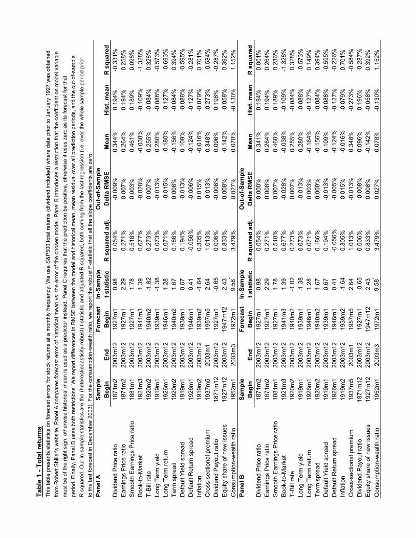
Table 1, whose format is based on the tables in Goyal and Welch, reports theresults. We begin by discussing panel A, and then discuss modifications to thebasic method reported in panels B, C, and D. Each row of the table considers

3

a different forecasting variable. The first four rows consider valuation ratios: thedividend price ratio, earnings price ratio, smoothed earnings price ratio, and book tomarket ratio. Each of these ratios has some accounting measure of corporate valuein the numerator, and market value in the denominator. The smoothed earningsprice ratio, proposed by Campbell and Shiller (1988b, 1998) is the ratio of a 10-year moving average of earnings to current prices. Campbell and Shiller argue thatthis ratio should have better forecasting power than the current earnings price ratiobecause aggregate corporate earnings display short-run cyclical noise; in particularearnings drop close to zero in recession years such as 1934 and 1992, creating spikes inthe current earnings price ratio that have nothing to do with stock market valuationlevels.2

The next seven rows consider nominal interest rates and inflation: the short-terminterest rate, long-term bond yield, lagged long-term bond return, the term spreadbetween long- and short-term Treasury yields, the default spread between corporateand Treasury bond yields, the lagged excess return on corporate over Treasury bonds,and the lagged rate of inflation.

The last four rows of the table evaluate forecasting variables that have beenproposed more recently: the cross-sectional beta premium of Polk, Thompson, andVuolteenaho (2003), the dividend payout ratio proposed by Lamont (1998), the equityshare of new issues proposed by Baker and Wurgler (2000), and the consumption-wealth ratio of Lettau and Ludvigson (2001). This last variable is based on a coin-tegrating relationship between consumption, aggregate labor income, and aggregatefinancial wealth. Rather than estimate a separate cointegrating regression, we simplyinclude the three variables directly in the forecasting equation for stock returns.

The first column of Table 1 reports the first date at which we have data to runthe forecasting regression. For dividends, earnings, and stock returns we have data,originally assembled by Robert Shiller, back to 1871. Other data series typicallybegin shortly after the end of World War I. All data series continue to the end of2003 as reported in the second column of the table. The third column reports thedate at which we begin the out-of-sample forecast evaluation. This is the beginningof 1927, when accurate data on total monthly stock returns become available from

2Goyal and Welch consider these variables, and also the ratio of lagged dividends to lagged prices(the “dividend yield” in Goyal and Welch’s terminology). We drop this variable as there is noreason to believe that it should predict better than the ratio of lagged dividends to current prices(the “dividend price ratio”).

4

CRSP, or 20 years after the date in column 1, whichever comes later.

The fourth and fifth columns of Table 1 report the full-sample t statistic for thesignificance of each variable in forecasting stock returns, and the adjusted R2 statisticof the full-sample regression.3 It is immediately obvious from the column of t sta-tistics that many of the valuation ratios and interest-rate variables are statisticallyinsignificant in predicting stock returns over this long sample period. The most suc-cessful variables are the two variants of the earnings price ratio, the Treasury bill rate,and the inflation rate. It may not be surprising that interest-rate variables are weakpredictors over the sample periods used here, as interest-rate behavior changed radi-cally in the early 1950’s when the modern era of monetary policy began. The threerecently proposed variables are much more successful return predictors in-sample,with t statistics of at least 2.4.

The remaining columns of the table evaluate the out-of-sample performance ofthese forecasts. The sixth column, labelled “Delta RMSE”, reports the difference inthe root mean squared error between the predictive regression and a forecast equalto the historical average return measured at each date (equivalent to a regressionof stock returns onto a constant). When this difference is negative, the historicalaverage return beats the predictive regression out of sample.

The seventh and eighth columns report the mean out-of-sample residual for thepredictive regression and the historical average return forecast. In the first few rowsof the table, which have initial data from the late 19th and early 20th centuries andan out-of-sample period starting in 1927, these residuals are typically positive. Thisreflects the strong performance of the US stock market in the later 20th Century.In rows corresponding to slowly moving valuation ratios such as the dividend-priceand earnings-price ratios, and also in the cross-sectional premium row, the residualsare more positive for the predictive regression than for the historical average return,reflecting the tendency of these variables to generate pessimistic return forecasts to-wards the end of the 20th Century.

The last column reports an out-of-sample R2 statistic that can be compared with3The adjustment of the R2 statistic for degrees of freedom makes only a very small difference in

samples of the size used here. For a regression from 1871 through 2003, the adjustment is -0.06%,and it is -0.11% for a regression from 1927 through 2003.

5

the in-sample R2 statistic. This is computed as

R2OS = 1−PT

t=1(rt − brt)2PTt=1(rt − rt)2

, (1)

where brt is the fitted value from a predictive regression estimated through periodt − 1, and rt is the historical average return estimated through period t − 1. Theout-of-sample R2 has the same sign as the change in the root mean squared errorreported in column 6, but it is measured in the same units as the in-sample R2 incolumn 5.

The out-of-sample performance of the predictor variables is quite mixed. PanelA of Table 1 shows that only two out of four valuation ratios, three out of seveninterest-rate variables, and two out of four recently proposed variables deliver positiveout-of-sample R2 statistics.

It is premature, however, to conclude with Goyal and Welch that predictive re-gressions cannot profitably be used by investors in real time. A regression estimatedover a short sample period can easily generate perverse results, such as a negativecoefficient when theory suggests that the coefficient should be positive. Since out-of-sample forecast evaluation begins as little as 20 years after the start of the data set,this can be an important problem in practice. For example, in the early 1930s theearnings-price ratio was very high, but the coefficient on the predictor was estimatedto be negative. This led to a negative forecast of the equity premium in the early1930s and subsequent poor forecast performance. In practice, an investor would notuse a perverse coefficient but would likely conclude that the coefficient is zero, ineffect imposing prior knowledge on the output of the regression.

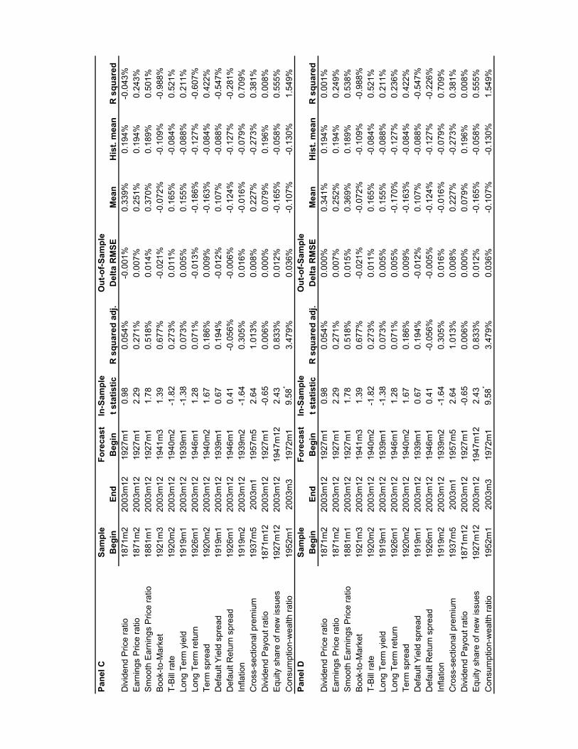
In panels B, C, and D we explore the impact of imposing sensible restrictions onthe out-of-sample forecasting exercise. In panel B we set the regression coefficientto zero whenever it has the “wrong” sign (different from the theoretically expectedsign estimated over the full sample). In panel C we assume that investors rule outa negative equity premium, and set the forecast to zero whenever it is negative. Wefollow the same procedure for the historical mean forecast, setting it to zero wheneverit is negative. In panel D we impose first the sign restriction on the coefficient, andthen the sign restriction on the forecast.

These restrictions improve the out-of-sample performance of predictive regressions.In panel A, as we noted above, only 2 out of 4 valuation ratios have a positive out-of-sample R2. In panels B and D this improves to 3 out of 4. Similarly, in panel A only

6

3 out of 7 interest-rate variables have a positive out-of-sample R2 statistic, but thisimproves to 4 out of 7 in panels B and C, and 5 out of 7 in panel D. The restrictionthat the equity premium be positive helps the performance of the cross-sectionalequity premium and the dividend payout ratio, so that all four recently proposedvariables have positive out-of-sample R2 in panels C and D. Importantly, once weimpose these restrictions the regressions that perform well out-of-sample now tendto be the ones that also work well in-sample. In fact the out-of-sample R2 in panelD sometimes exceeds the in-sample R2. The main exception is the book-to-marketratio, which generates a negative out-of-sample R2 statistic in all four panels of thetable.

Figure 1 illustrates the effect of the restrictions for the smoothed earnings-price ra-tio. The coefficient restriction significantly improves the forecasts in the 1930s, whenthe coefficient was estimated to be negative. The forecast restrictions are bindingduring the 1960s and 1990s, and improve the forecast performance during the 1990s.Valuation ratios were unusually low during these periods, leading to unprecedentedlylow forecasts. Campbell and Shiller (2001) also noted the unusually low earnings-price ratios of the 1990s, and wrote “We do not find this extreme forecast credible;when the independent variable has moved so far from the historically observed range,we cannot trust a linear regression line.” Our forecast restriction offers a simple wayto correct for this incredible forecast.

Looking at the performance of individual variables, it is striking how much betterthe earnings-based valuation ratios perform than the dividend-price ratio. This maywell be due to changes in payout policy as firms have shifted from paying dividends torepurchasing shares. Boudoukh, Michaely, Richardson, and Roberts (2004) empha-size that in recent years the total payout to price ratio, including share repurchases,has much stronger predictive power than the dividend-price ratio. Also, short- andlong-term Treasury yields perform reasonably well both in-sample and out-of-sample,consistent with the conclusion of Ang and Bekaert (2003) that these variables arerobust return predictors. The performance of these variables would be stronger ifwe started the sample period later, because the interest-rate process changed dra-matically at the time of the Federal Reserve-Treasury Accord in 1951. The recentlyproposed variables tend to perform well, particularly Lettau and Ludvigson’s combi-nation of consumption, income, and wealth; however it should be remembered thatthese variables may have been selected with the aid of a specification search basedon almost all the data used here, and this may give them an artificial advantage overpredictor variables that were proposed in the late 1980’s or before.

7

All the regressions we have reported predict simple stock returns rather than logstock returns. The use of simple returns makes little difference to the comparison ofpredictive regressions with historical mean forecasts, but all forecasts tend to generatehigher mean residuals when log returns are used. The reason for this is that highstock market volatility in the 1920’s and 1930’s depressed log returns relative to simplereturns in this period. Thus the gap between average stock returns in the late 20thCentury and the early 20th Century is greater when log returns are used.

3 How large an R2 should we expect?

In the previous section we showed that many of the forecasting variables that havebeen discussed in the literature do have positive out-of-sample predictive power foraggregate US stock returns, when reasonable restrictions are imposed on the predic-tive regression. However the R2 statistics are very small in magnitude. This raisesthe important question of whether they are economically meaningful.

To explore this issue, consider the following example:

rt+1 = µ+ xt + εt+1, (2)

where rt+1 is the excess simple return on a risky asset over the riskless interest rate, µis the unconditional average excess return, xt is a predictor variable with mean zero,and εt+1 is a random shock with mean zero. For tractability, consider an investorwith a single-period horizon and mean-variance preferences. The investor’s objectivefunction is expected portfolio return less (γ/2) times portfolio variance, where γ canbe interpreted as the coefficient of relative risk aversion.4 If the investor does notobserve xt, she chooses a portfolio weight in the risky asset

αt = α =

µ1

γ

¶µµ

σ2x + σ2ε

¶(3)

and earns an average excess return ofµ1

γ

¶µµ2

σ2x + σ2ε

¶=S2

γ, (4)

4Merton (1969) presents the analogous portfolio solution for the case where the investor has powerutility with relative risk aversion γ, asset returns are lognormally distributed, and the portfolio can becontinuously rebalanced. Campbell and Viceira (2002, Chapter 2) use a discrete-time approximateversion of Merton’s solution.

8

where S is the unconditional Sharpe ratio of the risky asset.

If the investor observes xt, she sets

αt =

µ1

γ

¶µµ+ xtσ2ε

¶, (5)

where the denominator is now σ2ε rather than σ2x + σ2ε because the variation in thepredictor variable xt is now expected and does not contribute to risk. The investorearns an average excess return ofµ

1

γ

¶µµ2 + σ2x

σ2ε

¶=

µ1

γ

¶µS2 +R2

1−R2¶, (6)

where

R2 =σ2x

σ2x + σ2ε(7)

is the R2 statistic for the regression of excess return on the predictor variable xt.

The difference between the two expected returns isµ1

γ

¶µR2

1−R2¶(1 + S2) (8)

which is always larger than R2/γ, and is close to R2/γ when the time interval is shortand R2 and S2 are both small. The proportional increase in the expected returnfrom observing xt is µ

R2

1−R2¶µ

1 + S2

S2

¶(9)

which is always larger than R2/S2 and is close to R2/S2 when the time interval isshort and R2 and S2 are both small.

This analysis shows that the right way to judge the magnitude of R2 is to compareit with the squared Sharpe ratio S2. If R2 is large relative to S2, then an investorcan use the information in the predictive regression to obtain a large proportionalincrease in portfolio return. In our monthly data since 1871, the monthly Sharperatio for stocks is 0.108, corresponding to an annual Sharpe ratio of 0.374. Thesquared monthly Sharpe ratio S2 = 0.012 = 1.2%. This can be compared with theout-of-sample R2 statistic for, say, the earnings-price ratio of 0.25% in Panel D ofTable 1. A mean-variance investor can use the earnings-price ratio to increase her

9

average monthly portfolio return by a proportional factor of 0.25/1.2 = 21%. Theabsolute increase in portfolio return depends on risk aversion, but is about 25 basispoints per month or 3% per year for an investor with unit risk aversion, and about 1%per year for an investor with a risk aversion coefficient of three. Predictor variables inTable 1 with higher out-of-sample R2 statistics imply correspondingly larger increasesin return.

The investor who observes xt gets a higher portfolio return in part by taking ongreater risk. Thus the increase in the average return is not pure welfare gain fora risk-averse investor. To take account of this, in Table 2 we calculate the welfarebenefits generated by optimally trading on each predictor variable for an investor withrelative risk aversion of three. We impose realistic portfolio constraints, preventingthe investor from shorting stocks or taking more than 50% leverage, that is, confiningthe portfolio weight on stocks to lie between 0 and 150%. The investor’s optimalportfolio depends on her estimate of stock return variance at each point in time, andwe consider two alternative assumptions about how the investor forms this estimate.In the central panel of the table, the investor estimates variance using all data availableup to the time her investment is made, while in the right hand panel, the investorestimates variance using a rolling five-year window of monthly data. The latterapproach may be more appropriate if the investor believes that there are short-termfluctuations in variance. We report the utility level from investing with the historicalmean forecast of the equity premium, and the changes in utility caused by investingwith the unrestricted linear regression of Table 1, Panel A, or the doubly restrictedlinear regression of Table 1, Panel D. These utility differences have the units ofexpected return, so they can also be interpreted as the transactions costs or portfoliomanagement fees that investors would be prepared to pay each month to exploit theinformation in the predictor variable.

In Table 2 the imposition of forecast restrictions makes less difference than it didin Table 1. The reason is that we rule out short sales, so investors are unable to act onnegative forecasts of the equity premium even if their predictive regressions generatesuch forecasts. The use of time-varying variance forecasts makes little difference forvaluation ratios or the recently proposed predictor variables, but it generally increasesthe utility gain from predicting stock returns with interest rates. Three out of seveninterest rates generate positive utility gains when a constant variance assumption isused, while six out of seven do so when a time-varying variance estimate is used.

The predictor variables that generate the highest out-of-sample R2 statistics gen-

10

erally deliver positive utility gains to investors. The main exception to this is thesmoothed earnings-price ratio, which has a positive out-of-sample R2 statistic but anegative utility gain. This result is driven by volatile monthly returns in the early1930’s, together with the diminishing marginal utility of risk-averse investors thatdownweights portfolio profits relative to losses. The smoothed earnings-price ra-tio increases utility if the evaluation period excludes the early 1930’s, or if a longerinvestment horizon is used as we discuss below.

The utility gains reported in Table 2 are limited by the leverage constraint, to-gether with the high average equity premium. Predictable variations in stock returnsdo not generate portfolio gains when there is a binding upper limit on equity invest-ment. Utility gains would be larger if we relaxed the portfolio constraint or includedadditional assets, with higher average returns than Treasury bills, in the portfoliochoice problem. On the other hand, Table 2 does not take any account of trans-actions costs. Modest gains from market timing strategies could be offset by theadditional costs implied by those strategies. Optimal trading strategies in the pres-ence of transactions costs are complex, and so we do not explore this issue furtherhere. We note that even the baseline strategy based on a historical-mean forecastincurs rebalancing costs and that utility gains of 10 basis points per month, or 1.2%per year, as reported in several rows of Table 2, are sufficient to cover substantialadditional costs.

Since small R2 statistics can generate large benefits for investors, we should expectpredictive regressions to have only modest explanatory power. Regressions with largeR2 statistics would be too profitable to believe. The saying “If you’re so smart,why aren’t you rich?” applies with great force here, and should lead investors tosuspect that highly successful predictive regressions are spurious. Note, however,that the squared Sharpe ratio and average real interest rate increase in proportionwith the investment horizon; thus much larger R2 statistics are believable at longerhorizons. Authors such as Fama and French (1988) have found that R2 statisticsincrease strongly with the horizon when the predictor variable is persistent, a findingthat is analyzed in Campbell, Lo, and MacKinlay (1997, Chapter 7) and Campbell(2001). This behavior is completely consistent with our analysis here.

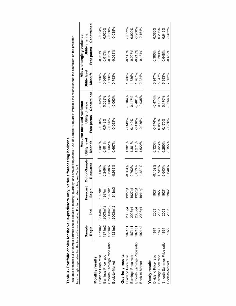
Table 3 illustrates the effect of increasing the investment horizon on the perfor-mance of our four valuation ratios. These predictor variables are highly persistent,so we would expect their explanatory power to increase as we change the horizonfrom one month in the top panel, to one quarter in the middle panel, to one year

11

in the bottom panel. Indeed the out-of-sample R2 statistics increase dramaticallyfor the two earnings-based ratios and become positive for the book-to-market ratio.However the forecasting performance of the dividend-price ratio does not improve atlonger horizons. The right hand part of Table 3 reports utility gains for these fourratios implemented at different horizons. The earnings-based ratios deliver solid im-provements when used to invest over one year, as does the dividend-price ratio whenthe investor allows for changing volatility of stock returns, but the book-to-marketratio does not improve utility despite its positive out-of-sample R2 at a one yearhorizon.

4 Reconciling in-sample with out-of-sample results

How do we reconcile apparent differences between in-sample and out-of-sample perfor-mance of the predictors? We emphasize that the differences are not typically large: InTable 1 small in-sample t statistics generally correspond to poor out-of-sample perfor-mance. However there are predictors, such as the book-to-market ratio, that displaystatistically significant t statistics along with inferior out-of-sample performance.

There are many reasons why out-of-sample evidence can contradict in-sampleresults. These include the effects of data mining, structural change, parameter uncer-tainty, and bad luck. Data mining occurs when a researcher evaluates several differentpredictors, but only reports those that are significant. This specification search canlead to spurious evidence of predictability. In principle out-of-sample analysis cancounter data mining, since a spurious predictor should not work out-of-sample. Ofcourse, the RMSE comparisons reported here and in Goyal and Welch (2004) are nottrue out-of-sample statistics. Just like the in-sample t statistics, they are functions ofhistorical data. To see this point more clearly, suppose that finance academics decidedto evaluate predictive relationships using RMSE comparisons instead of t statistics.A researcher could evaluate several different predictors, then choose to report onlythose that show large improvements in out-of-sample RMSE. So it seems unlikelythat data mining explains the different results.

Certain kinds of structural change can lead to spurious findings of in-sample pre-dictability (Clark and McCracken 2003, Giacomini and White 2003, Paye and Tim-mermann 2003). Suppose the predictive relationship is strong at the beginning ofthe sample but weakens over time. In this case the in-sample t statistic may detect

12

the strong relationship on average. However a market participant might not havebeen able to use the forecasting relationship, since at the beginning of the sample itwould be hard to estimate, and toward the end of the sample it would have disap-peared. While this represents a weakness of in-sample statistics, Inoue and Kilian(2004) have shown that out-of-sample statistics have the same problems. To continuethe example, if the predictive relationship declines slowly the out-of-sample statisticswill also detect past predictability. Inoue and Kilian (2004) argue that the relativeperformance of in-sample and out-of-sample statistics has a great deal to do with theform of structural change. Without a specific model of structural change, it is difficultto conclude which statistics are more useful to forecasters.

Next we turn to the effects of parameter uncertainty. To fix ideas, consider thepredictive regression

rt+1 = µ+ θxt + εt+1, (10)

with E εt = 0. rt is the excess return on the S&P 500 and xt is a predictor variablelike the dividend-price ratio. Should a forecaster use the historical mean or the fittedvalue brt+1 = bµ+ bθxt? If θ 6= 0 the historical mean of rt+1 will be a biased predictor,while brt+1 will be unbiased so long as the regression estimates are unbiased. On theother hand, estimation error for θ will increase the variance of brt+1 over the historicalmean. Thus there is a choice between the unbiased but noisy predictor brt+1 and thepossibly biased and less-noisy historical mean. If θ = 0, we expect the historicalmean to forecast more accurately since both predictors are unbiased while estimationerror for θ will add noise to the forecast. As θ increases the bias of the historicalmean becomes more important. However, if θ and the sample size are both small,then the noise from estimating θ may dominate the gains from eliminating the bias.In light of the bias-variance tradeoff, consider Inoue and Kilian’s (2004) result thatin-sample predictability tests are generally more powerful than out-of-sample tests.In some situations a powerful in-sample test could correctly detect predictability, butthat predictability could be useless to a market participant who cannot estimate thepredictive coefficient accurately enough to improve her forecast.

The bias-variance tradeoff becomes more complicated when the regression esti-mates are biased. This will occur when the predictor variable is persistent and shocksto the predictor are correlated with shocks to the market return. Following Stam-baugh (1999), we model the predictor with

xt+1 = ν + ρxt + ut+1 (11)

13

with Eut+1 = 0. Classical asymptotic theory states that in a large sample the ordinaryleast squares estimator for θ is unbiased and has the smallest sampling variabilityamong unbiased estimators. It is well known, however, that when ρ is close to 1and Corr (et+1, ut+1) is nonzero, classical asymptotics offers a poor approximation tothe true sampling distribution of the OLS estimator in small samples. For example,Stambaugh (1999) shows that when x is the dividend yield the OLS estimator and thein-sample t statistic are biased upward, leading to findings of spurious predictability.

These concerns about parameter uncertainty led us to impose the forecast restric-tions in Table 1. We required θ to have the theoretically correct sign, and we alsorequired the forecasted equity premium to be positive. This solution is not opti-mal, but there does not appear to exist an optimal forecaster when the predictor ispersistent. An unbiased estimator for θ does not exist, although Stambaugh (1999)and Amihud and Hurvich (2004) have developed bias corrections. Litterman (1986)encountered these issues when forecasting macroeconomic series. His solution wasto impose Bayesian prior information on θ. Our forecast restrictions can loosely bethought of as a uniform prior in a restricted part of the parameter space.

Finally, we turn to the problem of bad luck. Consider the unrealistic scenariowhere θ is known and nonzero. In this case a market participant will use the fore-casting variable xt since it improves her forecast in expectation. However, in a finitesample it may still be the case that the historical mean beats the forecasting variablewith known θ. This does not mean that the market participant should not use theforecasting variable. Rather she made the right decision but was unlucky.

We carried out a Monte Carlo experiment to assess the effects of parameter uncer-tainty and bad luck. For each predictor variable, we estimated equations (10) and (11)by ordinary least squares, and fit a constant-correlation GARCH model (Bollerslev1990) to the residuals.5 We then simulated 5000 data sets from the estimated mod-

5The error variances follow

σ2e,t = ω1 + α1e2t−1 + β1σ

2e,t−1; σ2u,t = ω2 + α2u

2t−1 + β2σ

2u,t−1

with σ2e,t ≡ Vart−1(et) and σ2u,t ≡ Vart−1(ut). The conditional correlations Corrt−1(et, ut) areconstant. Let (bet, but) denote residuals from regressions (10) and (11). We estimate the CC GARCHmodel by maximum likelihood, assuming the errors (et, ut) are bivariate normal. Bollerslev andWooldridge (1992) have shown that these parameter estimates will be consistent even if the trueerrors are not distributed bivariate normal. Our Monte Carlo simulations do not impose normality;rather they match the empirical distribution of the residuals (bet, but). Our algorithm for simulatingthe jth pair (ej , uj) follows. We normalize the residuals by their implied variances to obtain the

14

els, and for each simulated data set compared the out-of-sample forecasting resultsfrom using the historical mean to the results from using the predictor variable. Sincenone of the estimated values of θ are zero, all of the data generating processes implysome degree of predictability. The central panel of Table 4 reports the percentage ofsimulated data sets where the predictor variable leads to an inferior mean-squarederror forecast than the historical mean.

Table 4 shows that parameter uncertainty can have a large effect on out-of-sampleperformance. For example, the in-sample R2 statistic for the book-to-market ratiois 0.677%, yet at those in-sample parameter values the historical mean beats theunrestricted regression forecast in 35.5% of the simulations. The table also showsthat forecast restrictions lead to significant improvements on average. For predictionwith the inflation rate, the unrestricted regression forecast is inferior to the mean in54.4% of the draws, but once the restrictions are imposed that drops to 36.3%.

The table demonstrates that poor out-of-sample performance can also come frombad luck. The last column of the central panel of Table 4, labelled “known θ”,reports the infeasible results from using the true value of θ. Even when θ is known,the historical mean beats the forecasting variable in a surprisingly large number ofcases. For the book-to-market ratio, the historical mean is superior in almost 10% ofthe cases. Thus a strong “true” forecasting relationship can be associated with poorout-of-sample performance.

The right hand panel of Table 4 conducts a similar exercise for the utility gainsreported in Table 2. The first column in this panel reports the fraction of cases inwhich a portfolio, optimally constructed given a restricted linear regression, deliverslower average utility than a portfolio constructed using the historical equity-premiumforecast. Both portfolios are based on a 5-year rolling variance estimate for stockreturns. The second column reports the fraction of cases in which the investorunderperforms even though she knows the true coefficient of the linear regression.The results make it clear that prolonged underperformance is quite likely even whenstock returns can be stably predicted using the forecast variables discussed in therecent finance literature.

In unreported results we also calculated the percent of simulations where theout-of-sample R2 was smaller than the actual value in Table 1. Recall that the out-

empirical distribution of draws (bet/σe,t, but/σu,t). We randomly draw a pair from this unit-variancedistribution, then multiply the elements by the variances implied by the simulated Garch model.

15

of-sample R2 compares the forecast based on the predictive regression to the forecastbased on the historical mean, so a negative value implies that the historical mean issuperior. If the simulation percentages are very low, then the simulated data tend togenerate out-of-sample statistics which are larger than the ones we see in the data.This would suggest that the out-of-sample R2 values we see in the data are lower thanwhat we would expect based on the full sample parameter estimates. The simulationpercentages can be interpreted as p-values for the null hypothesis that the in-sampleand out-of-sample results are consistent with one another.

We computed 60 p-values, based on 15 predictors and four possible forecast re-strictions. The median p-value was 46.4%. P -values for the book-to-market ratioand default yield predictors range from 0.9% to 5.5%. Therefore these two predictorsgenerate unusually small out-of-sample R2 statistics given the full sample results. Forthe rest of the predictors the smallest p-value is 3.7%, for the long-term return withthe forecast restricted to be positive. All of the rest of the p-values are greater than5%. We conclude that for nearly all the predictors and various forecast restrictions,the out-of-sample R2 statistics in Table 1 are consistent with the in-sample t statisticsand R2 values.

These results shed light on an interesting question. Suppose a forecasting variablehas a significant t statistic, but has underperformed the historical mean out-of-sample.Should an investor use that variable in the future? On the one hand, poor out-of-sample performance could indicate the presence of structural breaks in the data, ordeleterious effects of parameter uncertainty. These factors suggest that investmentdecisions should not be based on this predictor variable. On the other hand, poorout-of-sample results could be due to bad luck. Also, since more data are availablenow, the effects of parameter uncertainty are less serious now than in the past. Theseconsiderations suggest that the investor should use the forecasting variable, relying onits in-sample predictive power. Without further theory or information this questiondoes not have a clear answer, but our results in Table 4 suggest that one should notexaggerate the significance of poor out-of-sample statistics.

16

5 Conclusion

A number of variables are correlated with subsequent returns on the aggregate USstock market in the 20th Century. Some of these variables are stock market valuationratios, others reflect the levels of short- and long-term interest rates, patterns incorporate finance or the cross-sectional pricing of individual stocks, or the level ofconsumption in relation to wealth. Amit Goyal and IvoWelch (2004) have argued thatin-sample correlations conceal a systematic failure of these variables out of sample:None are able to beat a simple forecast based on the historical average stock return.

In this note we have shown that most of these predictor variables, and almostall that are statistically significant in-sample, perform better out-of-sample than thehistorical average return forecast, once sensible restrictions are imposed on the signsof coefficients and return forecasts. The out-of-sample explanatory power is small,but nonetheless is economically meaningful for investors. We have also shown that avariable is quite likely to have poor out-of-sample performance for an extended periodof time even when the variable genuinely predicts returns with a stable coefficient.

17

References

Amihud, Yakov and Clifford Hurvich, 2004, Predictive regressions: a reduced-biasestimation method, forthcoming Journal of Financial and Quantitative Analy-sis.

Ang, Andrew and Geert Bekaert, 2003, Stock return predictability: Is it there?,unpublished paper, Columbia University.

Baker, Malcolm and Jeffrey Wurgler, 2000, The equity share in new issues andaggregate stock returns, Journal of Finance 55, 2219—2257.

Bollerslev, Tim, 1990, Modelling the coherence in short-run nominal exchange rates:a multivariate generalized ARCH model, Review of Economics and Statistics72, 498—505.

Bollerslev, Tim and Jeff Wooldridge 1992, Quasi-maximum likelihood estimationand inference in dynamic models with time-varying covariances, EconometricReviews 11, 143—172.

Boudoukh, Jacob, Roni Michaely, Matthew Richardson, and Michael Roberts, 2004,On the importance of measuring payout yield: Implications for empirical assetpricing, NBER Working Paper 10651.

Butler, Alexander W., Gustavo Grullon, and James P. Weston, 2004, Can managersforecast aggregate market returns?, unpublished paper, University of SouthFlorida and Rice University.

Campbell, John Y., 1987, Stock returns and the term structure, Journal of FinancialEconomics 18, 373—399.

Campbell, John Y., 2001, Why long horizons? A study of power against persistentalternatives, Journal of Empirical Finance 8, 459—491.

Campbell, John Y., Andrew W. Lo, and A. Craig MacKinlay, 1997, The Economet-rics of Financial Markets, Princeton University Press, Princeton, NJ.

Campbell, John Y. and Robert J. Shiller, 1988a, The dividend-price ratio and ex-pectations of future dividends and discount factors, Review of Financial Studies1, 195—228.

18

Campbell, John Y. and Robert J. Shiller, 1988b, Stock prices, earnings, and expecteddividends, Journal of Finance 43, 661—676.

Campbell, John Y. and Robert J. Shiller, 1998, Valuation ratios and the long-runstock market outlook, Journal of Portfolio Management.

Campbell, John Y. and Robert J. Shiller, 2001, Valuation ratios and the long-runstock market outlook: an update, NBER Working Paper 8221.

Campbell, John Y. and Luis M. Viceira, 2002, Strategic Asset Allocation: PortfolioChoice for Long-Term Investors, Oxford University Press, New York, NY.

Campbell, John Y. and Motohiro Yogo, 2003, Efficient tests of stock return pre-dictability, unpublished paper, Harvard University.

Cavanagh, Christopher L., Graham Elliott, and James H. Stock, 1995, Inference inmodels with nearly integrated regressors, Econometric Theory 11, 1131 —1147.

Clark, Todd E. and Michael W. McCracken, 2003, The power of tests of predictiveability in the presence of structural breaks, unpublished paper, Federal ReserveBank of Kansas City and University of Missouri-Columbia.

Fama, Eugene F. and Kenneth R. French, 1988, Dividend yields and expected stockreturns, Journal of Financial Economics 22, 3—25.

Fama, Eugene F. and Kenneth R. French, 1989, Business conditions and expectedreturns on stocks and bonds, Journal of Financial Economics 25, 23—49.

Fama, Eugene F. and G. William Schwert, 1977, Asset returns and inflation, Journalof Financial Economics 5, 115—146.

Ferson, Wayne E., Sergei Sarkissian, and Timothy T. Simin, 2003, Spurious regres-sions in financial economics?, Journal of Finance 58, 1393—1413.

Giacomini, Raffaella and Halbert White, Tests of conditional predictive ability, un-published paper, University of California at Los Angeles and University of Cal-ifornia at San Diego.

Goyal, Amit and Ivo Welch, 2003, Predicting the equity premium with dividendratios, Management Science 49, 639—654.

19

Goyal, Amit and Ivo Welch, 2004, A comprehensive look at the empirical perfor-mance of equity premium prediction, NBER Working Paper 10483.

Graham, Benjamin and David L. Dodd, 1934, Security Analysis, first edition, Mc-Graw Hill, New York, NY.

Hodrick, Robert J., 1992, Dividend yields and expected stock returns: Alternativeprocedures for inference and measurement, Review of Financial Studies 5, 257—286.

Inoue, Atsushi and Lutz Kilian, 2004, In-sample or out-of-sample tests of predictabil-ity: which one should we use?, forthcoming Econometric Reviews.

Jansson, Michael, and Marcelo J. Moreira, 2003, Optimal inference in regressionmodels with nearly integrated regressors, unpublished paper, Harvard Univer-sity.

Keim, Donald B. and Robert F. Stambaugh, 1986, Predicting returns in the stockand bond markets, Journal of Financial Economics 17, 357—390.

Kilian, Lutz, 1999, Exchange rates and monetary fundamentals: What do we learnfrom long-horizon regressions?, Journal of Applied Econometrics 14, 491—510.

Kothari, S.P. and Jay Shanken, 1997, Book-to-market, dividend yield, and expectedmarket returns: A time-series analysis, Journal of Financial Economics 44, 169—203.

Lamont, Owen, 1998, Earnings and expected returns, Journal of Finance 53, 1563—1587.

Lettau, Martin and Sydney Ludvigson, 2001, Consumption, aggregate wealth, andexpected stock returns, Journal of Finance 56, 815—849.

Lewellen, Jonathan, 2004, Predicting returns with financial ratios, Journal of Fi-nancial Economics 74, 209—235.

Litterman, Robert, 1986, Forecasting with Bayesian vector autoregressions: Fiveyears of experience, Journal of Business & Economic Statistics 4, 25—38.

Mark, Nelson C., 1995, Exchange rates and fundamentals: Evidence on long-horizonpredictability, American Economic Review 85, 201—218.

20

Merton, Robert C., 1969, Lifetime portfolio selection under uncertainty: the contin-uous time case, Review of Economics and Statistics 51, 247—257.

Paye, Bradley and Alan Timmermann, 2003, Instability of return prediction models,unpublished paper, University of California at San Diego.

Polk, Christopher, Samuel Thompson, and TuomoVuolteenaho, 2005, Cross-sectionalforecasts of the equity premium, forthcoming, Journal of Financial Economics.

Pontiff, Jeffrey and Lawrence D. Schall, 1998, Book-to-market ratios as predictorsof market returns, Journal of Financial Economics 49, 141—160.

Rozeff, Michael S., 1984, Dividend yields are equity risk premiums, Journal of Port-folio Management 11(1), 68—75.

Stambaugh, Robert F., 1999, Predictive regressions, Journal of Financial Economics54, 375—421.

Torous, Walter, Rossen Valkanov, and Shu Yan, 2004, On predicting stock returnswith nearly integrated explanatory variables, Journal of Business 77, 937—966.

21

Tabl

e 1

- Tot

al re

turn

sTh

is ta

ble

pres

ents

sta

tistic

s on

fore

cast

err

ors

for s

tock

retu

rns

at a

mon

thly

freq

uenc

y. W

e us

e S

&P

500

tota

l ret

urns

(div

iden

d in

clud

ed) w

here

dat

a pr

ior t

o Ja

nuar

y 19

27 w

as o

btai

ned

from

Rob

ert S

hille

r's w

ebsi

te. P

anel

A c

ompa

res

fore

cast

err

or o

f his

toric

al m

ean

vs. t

he e

rror

of t

he c

hose

n m

odel

. Pan

el B

intro

duce

s a

rest

rictio

n th

at th

e co

effic

ient

on

mod

el v

aria

ble

mus

t be

of th

e rig

ht s

ign,

oth

erw

ise

hist

oric

al m

ean

is u

sed

as a

pre

dict

or in

stea

d. P

anel

C re

quire

s th

at th

e pr

edic

tion

be p

ositi

ve, o

ther

wis

e it

uses

zer

o as

its

fore

cast

for t

hat

perio

d. F

inal

ly, P

anel

D u

ses

both

rest

rictio

ns. W

e re

port

diffe

renc

es in

RM

SE

bet

wee

n th

e m

odel

and

his

toric

al m

ean,

mea

n re

sidu

al o

ver a

ll pr

edic

tion

perio

ds, a

nd th

e ou

t-of-s

ampl

eR

squ

ared

. Our

in-s

ampl

e st

atis

tics

are

the

(het

eros

keda

stic

ity-r

obus

t) t-s

tatis

tic a

nd a

djus

ted

R s

quar

ed, b

oth

com

ing

from

the

last

regr

essi

on (i

.e. o

ver t

he w

hole

sam

ple

perio

d pr

ior

to th

e la

st fo

reca

st in

Dec

embe

r 200

3). F

or th

e co

nsum

ptio

n-w

ealth

ratio

, we

repo

rt th

e ro

bust

F-s

tatis

tic th

at a

ll th

e sl

ope

coef

ficie

nts

are

zero

.Pa

nel A

Sam

ple

Fore

cast

In-S

ampl

eO

ut-o

f-Sam

ple

Beg

inEn

dB

egin

t sta

tistic

R s

quar

ed a

dj.

Del

ta R

MSE

Mea

nH

ist.

mea

nR

squ

ared

Div

iden

d P

rice

ratio

1871

m2

2003

m12

1927

m1

0.98

0.05

4%-0

.009

%0.

344%

0.19

4%-0

.331

%E

arni

ngs

Pric

e ra

tio18

71m

220

03m

1219

27m

12.

290.

271%

0.00

7%0.

264%

0.19

4%0.

258%

Sm

ooth

Ear

ning

s P

rice

ratio

1881

m1

2003

m12

1927

m1

1.78

0.51

8%0.

003%

0.46

1%0.

189%

0.09

8%B

ook-

to-M

arke

t19

21m

320

03m

1219

41m

31.

390.

677%

-0.0

28%

-0.0

38%

-0.1

09%

-1.3

28%

T-B

ill ra

te19

20m

220

03m

1219

40m

2-1

.82

0.27

3%0.

007%

0.25

5%-0

.084

%0.

328%

Long

Ter

m y

ield

1919

m1

2003

m12

1939

m1

-1.3

80.

073%

-0.0

13%

0.28

0%-0

.088

%-0

.573

%Lo

ng T

erm

retu

rn19

26m

120

03m

1219

46m

11.

280.

071%

-0.0

15%

-0.1

80%

-0.1

27%

-0.6

93%

Term

spr

ead

1920

m2

2003

m12

1940

m2

1.67

0.18

6%0.

008%

-0.1

56%

-0.0

84%

0.39

4%D

efau

lt Y

ield

spr

ead

1919

m1

2003

m12

1939

m1

0.67

0.19

4%-0

.013

%0.

109%

-0.0

88%

-0.5

95%

Def

ault

Ret

urn

spre

ad19

26m

120

03m

1219

46m

10.

41-0

.056

%-0

.006

%-0

.124

%-0

.127

%-0

.281

%In

flatio

n19

19m

220

03m

1219

39m

2-1

.64

0.30

5%0.

015%

-0.0

16%

-0.0

79%

0.70

1%C

ross

-sec

tiona

l pre

miu

m19

37m

520

03m

119

57m

52.

641.

013%

-0.0

13%

0.34

8%-0

.273

%-0

.584

%D

ivid

end

Pay

out r

atio

1871

m12

2003

m12

1927

m1

-0.6

50.

006%

-0.0

08%

0.09

6%0.

196%

-0.2

87%

Equ

ity s

hare

of n

ew is

sues

1927

m12

2003

m12

1947

m12

2.43

0.83

3%0.

008%

-0.1

42%

-0.0

58%

0.39

2%C

onsu

mpt

ion-

wea

lth ra

tio19

52m

120

03m

319

72m

19.

58*

3.47

9%0.

027%

0.07

8%-0

.130

%1.

152%

Pane

l BSa

mpl

eFo

reca

stIn

-Sam

ple

Out

-of-S

ampl

eB

egin

End

Beg

int s

tatis

ticR

squ

ared

adj

.D

elta

RM

SEM

ean

His

t. m

ean

R s

quar

edD

ivid

end

Pric

e ra

tio18

71m

220

03m

1219

27m

10.

980.

054%

0.00

0%0.

341%

0.19

4%0.

001%

Ear

ning

s P

rice

ratio

1871

m2

2003

m12

1927

m1

2.29

0.27

1%0.

008%

0.26

4%0.

194%

0.26

4%S

moo

th E

arni

ngs

Pric

e ra

tio18

81m

120

03m

1219

27m

11.

780.

518%

0.00

7%0.

460%

0.18

9%0.

236%

Boo

k-to

-Mar

ket

1921

m3

2003

m12

1941

m3

1.39

0.67

7%-0

.028

%-0

.038

%-0

.109

%-1

.328

%T-

Bill

rate

1920

m2

2003

m12

1940

m2

-1.8

20.

273%

0.00

7%0.

255%

-0.0

84%

0.32

8%Lo

ng T

erm

yie

ld19

19m

120

03m

1219

39m

1-1

.38

0.07

3%-0

.013

%0.

280%

-0.0

88%

-0.5

73%

Long

Ter

m re

turn

1926

m1

2003

m12

1946

m1

1.28

0.07

1%0.

003%

-0.1

64%

-0.1

27%

0.14

9%Te

rm s

prea

d19

20m

220

03m

1219

40m

21.

670.

186%

0.00

8%-0

.156

%-0

.084

%0.

394%

Def

ault

Yie

ld s

prea

d19

19m

120

03m

1219

39m

10.

670.

194%

-0.0

13%

0.10

9%-0

.088

%-0

.595

%D

efau

lt R

etur

n sp

read

1926

m1

2003

m12

1946

m1

0.41

-0.0

56%

-0.0

05%

-0.1

24%

-0.1

27%

-0.2

26%

Infla

tion

1919

m2

2003

m12

1939

m2

-1.6

40.

305%

0.01

5%-0

.016

%-0

.079

%0.

701%

Cro

ss-s

ectio

nal p

rem

ium

1937

m5

2003

m1

1957

m5

2.64

1.01

3%-0

.013

%0.

348%

-0.2

73%

-0.5

84%

Div

iden

d P

ayou

t rat

io18

71m

1220

03m

1219

27m

1-0

.65

0.00

6%-0

.008

%0.

096%

0.19

6%-0

.287

%E

quity

sha

re o

f new

issu

es19

27m

1220

03m

1219

47m

122.

430.

833%

0.00

8%-0

.142

%-0

.058

%0.

392%

Con

sum

ptio

n-w

ealth

ratio

1952

m1

2003

m3

1972

m1

9.58

*3.

479%

0.02

7%0.

078%

-0.1

30%

1.15

2%

Pane

l CSa

mpl

eFo

reca

stIn

-Sam

ple

Out

-of-S

ampl

eB

egin

End

Beg

int s

tatis

ticR

squ

ared

adj

.D

elta

RM

SEM

ean

His

t. m

ean

R s

quar

edD

ivid

end

Pric

e ra

tio18

71m

220

03m

1219

27m

10.

980.

054%

-0.0

01%

0.33

9%0.

194%

-0.0

43%

Ear

ning

s P

rice

ratio

1871

m2

2003

m12

1927

m1

2.29

0.27

1%0.

007%

0.25

1%0.

194%

0.24

3%S

moo

th E

arni

ngs

Pric

e ra

tio18

81m

120

03m

1219

27m

11.

780.

518%

0.01

4%0.

370%

0.18

9%0.

501%

Boo

k-to

-Mar

ket

1921

m3

2003

m12

1941

m3

1.39

0.67

7%-0

.021

%-0

.072

%-0

.109

%-0

.988

%T-

Bill

rate

1920

m2

2003

m12

1940

m2

-1.8

20.

273%

0.01

1%0.

165%

-0.0

84%

0.52

1%Lo

ng T

erm

yie

ld19

19m

120

03m

1219

39m

1-1

.38

0.07

3%0.

005%

0.15

5%-0

.088

%0.

211%

Long

Ter

m re

turn

1926

m1

2003

m12

1946

m1

1.28

0.07

1%-0

.013

%-0

.186

%-0

.127

%-0

.607

%Te

rm s

prea

d19

20m

220

03m

1219

40m

21.

670.

186%

0.00

9%-0

.163

%-0

.084

%0.

422%

Def

ault

Yie

ld s

prea

d19

19m

120

03m

1219

39m

10.

670.

194%

-0.0

12%

0.10

7%-0

.088

%-0

.547

%D

efau

lt R

etur

n sp

read

1926

m1

2003

m12

1946

m1

0.41

-0.0

56%

-0.0

06%

-0.1

24%

-0.1

27%

-0.2

81%

Infla

tion

1919

m2

2003

m12

1939

m2

-1.6

40.

305%

0.01

6%-0

.016

%-0

.079

%0.

709%

Cro

ss-s

ectio

nal p

rem

ium

1937

m5

2003

m1

1957

m5

2.64

1.01

3%0.

008%

0.22

7%-0

.273

%0.

381%

Div

iden

d P

ayou

t rat

io18

71m

1220

03m

1219

27m

1-0

.65

0.00

6%0.

000%

0.07

9%0.

196%

0.00

8%E

quity

sha

re o

f new

issu

es19

27m

1220

03m

1219

47m

122.

430.

833%

0.01

2%-0

.165

%-0

.058

%0.

555%

Con

sum

ptio

n-w

ealth

ratio

1952

m1

2003

m3

1972

m1

9.58

*3.

479%

0.03

6%-0

.107

%-0

.130

%1.

549%

Pane

l DSa

mpl

eFo

reca

stIn

-Sam

ple

Out

-of-S

ampl

eB

egin

End

Beg

int s

tatis

ticR

squ

ared

adj

.D

elta

RM

SEM

ean

His

t. m

ean

R s

quar

edD

ivid

end

Pric

e ra

tio18

71m

220

03m

1219

27m

10.

980.

054%

0.00

0%0.

341%

0.19

4%0.

001%

Ear

ning

s P

rice

ratio

1871

m2

2003

m12

1927

m1

2.29

0.27

1%0.

007%

0.25

2%0.

194%

0.24

9%S

moo

th E

arni

ngs

Pric

e ra

tio18

81m

120

03m

1219

27m

11.

780.

518%

0.01

5%0.

369%

0.18

9%0.

538%

Boo

k-to

-Mar

ket

1921

m3

2003

m12

1941

m3

1.39

0.67

7%-0

.021

%-0

.072

%-0

.109

%-0

.988

%T-

Bill

rate

1920

m2

2003

m12

1940

m2

-1.8

20.

273%

0.01

1%0.

165%

-0.0

84%

0.52

1%Lo

ng T

erm

yie

ld19

19m

120

03m

1219

39m

1-1

.38

0.07

3%0.

005%

0.15

5%-0

.088

%0.

211%

Long

Ter

m re

turn

1926

m1

2003

m12

1946

m1

1.28

0.07

1%0.

005%

-0.1

70%

-0.1

27%

0.23

6%Te

rm s

prea

d19

20m

220

03m

1219

40m

21.

670.

186%

0.00

9%-0

.163

%-0

.084

%0.

422%

Def

ault

Yie

ld s

prea

d19

19m

120

03m

1219

39m

10.

670.

194%

-0.0

12%

0.10

7%-0

.088

%-0

.547

%D

efau

lt R

etur

n sp

read

1926

m1

2003

m12

1946

m1

0.41

-0.0

56%

-0.0

05%

-0.1

24%

-0.1

27%

-0.2

26%

Infla

tion

1919

m2

2003

m12

1939

m2

-1.6

40.

305%

0.01

6%-0

.016

%-0

.079

%0.

709%

Cro

ss-s

ectio

nal p

rem

ium

1937

m5

2003

m1

1957

m5

2.64

1.01

3%0.

008%

0.22

7%-0

.273

%0.

381%

Div

iden

d P

ayou

t rat

io18

71m

1220

03m

1219

27m

1-0

.65

0.00

6%0.

000%

0.07

9%0.

196%

0.00

8%E

quity

sha

re o

f new

issu

es19

27m

1220

03m

1219

47m

122.

430.

833%

0.01

2%-0

.165

%-0

.058

%0.

555%

Con

sum

ptio

n-w

ealth

ratio

1952

m1

2003

m3

1972

m1

9.58

*3.

479%

0.03

6%-0

.107

%-0

.130

%1.

549%

Tabl

e 2

- Por

tfolio

cho

ice

This

tabl

e pr

esen

ts o

ut-o

f-sam

ple

portf

olio

cho

ice

resu

lts a

t a m

onth

ly fr

eque

ncy.

"Out

-of-S

ampl

e R

-squ

ared

" com

es fr

om P

anel

D o

f Tab

le 1

. "A

ssum

e co

nsta

nt v

aria

nce"

resu

ltsca

lcul

ate

the

varia

nce

from

the

entir

e av

aila

ble

hist

ory

of e

xces

s re

turn

s. "A

llow

cha

ngin

g va

rianc

e" re

sults

cal

cula

te th

e va

rianc

e fro

m a

rolli

ng w

indo

w o

f the

last

5 y

ears

of d

ata.

"Util

ity le

vel,

mea

n fc

" is

the

aver

age

valu

e of

the

utili

ty fr

om fo

reca

stin

g th

e m

arke

t with

the

hist

oric

al m

ean.

"Util

ity c

hang

e" is

the

chan

ge in

ave

rage

util

ity fr

om fo

reca

stin

g th

e m

arke

t with

the

pred

icto

r ins

tead

of t

he h

isto

rical

mea

n. "F

ree

parm

s" in

dica

tes

that

we

used

the

unco

nstra

ined

ols

pre

dict

or o

f the

equ

ity p

rem

ium

(fro

m P

anel

A o

f Tab

le 1

)."C

onst

rain

ed" i

ndic

ates

that

we

cons

train

the

coef

ficie

nt o

n th

e pr

edic

tor t

o be

the

right

sig

n, a

nd w

e re

quire

that

the

pred

ictio

n be

non

-neg

ativ

e (fr

om P

anel

D o

f Tab

le 1

).Th

e ut

ility

func

tion

is E

(Rp)

- (γ

/2)V

ar(R

p), w

here

Rp

is th

e po

rtfol

io re

turn

and

γ=3

.

Sam

ple

Fore

cast

Out

-of-S

ampl

eU

tility

leve

lU

tility

leve

lB

egin

End

Beg

inR

squ

ared

Mea

n fc

Free

par

ms

Con

stra

ined

Mea

n fc

Free

par

ms

Con

stra

ined

Div

iden

d P

rice

ratio

1871

m2

2003

m12

1927

m1

0.00

1%0.

501%

-0.0

16%

-0.0

24%

0.66

0%-0

.037

%-0

.024

%E

arni

ngs

Pric

e ra

tio18

71m

220

03m

1219

27m

10.

249%

0.50

1%0.

048%

0.05

3%0.

660%

0.01

7%0.

020%

Sm

ooth

Ear

ning

s P

rice

ratio

1881

m1

2003

m12

1927

m1

0.53

8%0.

502%

-0.0

95%

-0.0

85%

0.66

0%-0

.053

%-0

.050

%B

ook-

to-M

arke

t19

21m

320

03m

1219

41m

3-0

.988

%0.

667%

-0.0

63%

-0.0

63%

0.79

3%-0

.038

%-0

.038

%T-

Bill

rate

1920

m2

2003

m12

1940

m2

0.52

1%0.

639%

-0.0

08%

-0.0

08%

0.77

1%0.

117%

0.11

7%Lo

ng T

erm

yie

ld19

19m

120

03m

1219

39m

10.

211%

0.62

6%-0

.021

%-0

.021

%0.

753%

0.08

6%0.

086%

Long

Ter

m re

turn

1926

m1

2003

m12

1946

m1

0.23

6%0.

641%

0.00

7%0.

040%

0.76

7%0.

015%

0.06

0%Te

rm s

prea

d19

20m

220

03m

1219

40m

20.

422%

0.63

9%0.

088%

0.08

8%0.

771%

0.13

1%0.

131%

Def

ault

Yie

ld s

prea

d19

19m

120

03m

1219

39m

1-0

.547

%0.

626%

-0.0

73%

-0.0

73%

0.75

3%-0

.075

%-0

.075

%D

efau

lt R

etur

n sp

read

1926

m1

2003

m12

1946

m1

-0.2

26%

0.64

1%-0

.014

%-0

.009

%0.

767%

0.01

0%0.

013%

Infla

tion

1919

m2

2003

m12

1939

m2

0.70

9%0.

630%

0.05

1%0.

051%

0.75

9%0.

108%

0.10

8%C

ross

-sec

tiona

l pre

miu

m19

37m

520

03m

119

57m

50.

381%

0.61

1%0.

010%

0.01

0%0.

621%

0.05

7%0.

057%

Div

iden

d P

ayou

t rat

io18

71m

1220

03m

1219

27m

10.

008%

0.50

2%0.

094%

0.09

4%0.

659%

0.01

2%0.

012%

Equ

ity s

hare

of n

ew is

sues

1927

m12

2003

m12

1947

m12

0.55

5%0.

649%

0.10

2%0.

102%

0.82

6%0.

128%

0.12

8%C

onsu

mpt

ion-

wea

lth ra

tio19

52m

120

03m

319

72m

11.

549%

0.53

3%0.

379%

0.37

9%0.

655%

0.30

0%0.

300%

Ass

ume

cons

tant

var

ianc

eA

llow

cha

ngin

g va

rianc

eU

tility

cha

nge

Util

ity c

hang

e

Tabl

e 3

- Por

tfolio

cho

ice

for t

he v

alue

-pre

dict

ors

only

, var

ious

fore

cast

ing

horiz

ons

This

tabl

e pr

esen

ts o

ut-o

f-sam

ple

portf

olio

cho

ice

resu

lts a

t mon

thly

, qua

rterly

, and

ann

ual f

requ

enci

es. "

Out

-of-S

ampl

e R

-squ

ared

" im

pose

s th

e re

stric

tion

that

the

coef

ficie

nt o

n th

e pr

edic

tor

has

the

right

sig

n, a

lso

that

the

fore

cast

is n

onne

gativ

e. F

or fu

rther

tabl

e no

tes,

see

Tab

le 2

.

Sam

ple

Fore

cast

Out

-of-S

ampl

eU

tility

leve

lU

tility

leve

lB

egin

End

Beg

inR

squ

ared

Mea

n fc

Free

par

ms

Con

stra

ined

Mea

n fc

Free

par

ms

Con

stra

ined

Mon

thly

resu

ltsD

ivid

end

Pric

e ra

tio18

71m

220

03m

1219

27m

10.

001%

0.50

1%-0

.016

%-0

.024

%0.

660%

-0.0

37%

-0.0

24%

Ear

ning

s P

rice

ratio

1871

m2

2003

m12

1927

m1

0.24

9%0.

501%

0.04

8%0.

053%

0.66

0%0.

017%

0.02

0%S

moo

th E

arni

ngs

Pric

e ra

tio18

81m

120

03m

1219

27m

10.

538%

0.50

2%-0

.095

%-0

.085

%0.

660%

-0.0

53%

-0.0

50%

Boo

k-to

-Mar

ket

1921

m3

2003

m12

1941

m3

-0.9

88%

0.66

7%-0

.063

%-0

.063

%0.

793%

-0.0

38%

-0.0

38%

Qua

rter

ly re

sults

Div

iden

d P

rice

ratio

1871

q120

03q4

1927

q1-0

.004

%1.

301%

-0.1

43%

-0.1

04%

1.78

6%-0

.145

%-0

.092

%E

arni

ngs

Pric

e ra

tio18

71q1

2003

q419

27q1

0.76

3%1.

301%

0.14

0%0.

147%

1.78

6%-0

.007

%0.

000%

Sm

ooth

Ear

ning

s P

rice

ratio

1871

q120

03q4

1927

q10.

613%

1.27

1%-0

.418

%-0

.401

%1.

767%

-0.2

13%

-0.2

08%

Boo

k-to

-Mar

ket

1921

q220

03q4

1941

q2-1

.630

%1.

622%

-0.0

35%

-0.0

35%

2.22

1%-0

.161

%-0

.161

%

Year

ly re

sults

Div

iden

d P

rice

ratio

1871

2003

1927

-0.1

59%

6.32

3%-0

.474

%-0

.474

%5.

947%

0.38

5%0.

385%

Ear

ning

s P

rice

ratio

1871

2003

1927

1.73

1%6.

323%

0.08

9%0.

122%

5.94

7%0.

290%

0.29

8%S

moo

th E

arni

ngs

Pric

e ra

tio18

8120

0319

276.

643%

6.28

0%0.

170%

0.17

0%5.

883%

0.64

8%0.

648%

Boo

k-to

-Mar

ket

1922

2003

1942

0.64

0%8.

155%

-0.2

56%

-0.2

56%

7.80

2%-0

.462

%-0

.462

%

Ass

ume

cons

tant

var

ianc

eA

llow

cha

ngin

g va

rianc

eU

tility

cha

nge

Util

ity c

hang

e

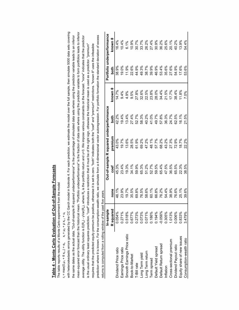
Tabl

e 4

- Mon

te C

arlo

Eva

luat

ion

of O

ut-o

f-Sam

ple

Fore

cast

sTh

e ta

ble

repo

rts re

sults

of a

Mon

te C

arlo

exp

erim

ent f

rom

the

mod

elr t

= m

ax(0

,µ1 +

θ x

t-1) +

et,

x

t = µ

2 + ρ

xt-1

+ u

t

with

het

eros

keda

stic

err

ors

gene

rate

d by

the

CC

Gar

ch m

odel

in fo

otno

te 4

. For

eac

h pr

edic

tor,

we

estim

ate

the

mod

el o

ver t

he fu

ll sa

mpl

e, th

en s

imul

ate

5000

dat

a se

ts c

over

ing

the

sam

e da

tes

as th

e ac

tual

dat

a. "O

ut-o

f-sam

ple

R s

quar

ed u

nder

perfo

rman

ce" i

s th

e pe

rcen

tage

of s

imul

ated

dat

a se

ts w

here

usi

ng th

e pr

edic

tor v

aria

ble

lead

s to

an

infe

rior

mea

n-sq

uare

d er

ror f

orec

ast t

han

the

hist

oric

al m

ean.

"Por

tfolio

und

erpe

rform

ance

" is

the

fract

ion

of d

ata

sets

whe

re u

sing

the

pred

icto

r var

iabl

e to

form

por

tfolio

s le

ads

to in

ferio

rav

erag

e ut

ility

. The

util

ity fu

nctio

n is

E(R

p) - γV

ar(R

p), w

here

Rp i

s th

e po

rtfol

io re

turn

and

γ=3

. We

impo

se v

ario

us c

onst

rain

ts o

n th

e fo

reca

st. "

none

" ind

icat

es th

at th

e pr

edic

tor

is th

e us

ual o

rdin

ary

leas

t squ

ares

pre

dict

ion.

"coe

f" in

trodu

ces

a re

stric

tion

that

θ m

ust b

e of

the

right

sig

n, o

thew

ise

the

hist

oric

al m

ean

is u

sed

as a

pre

dict

or. "

prem

ium

"re

quire

s th

at th

e pr

edic

ted

equi

ty p

rem

ium

be

posi

tive,

oth

erw

ise

it is

set

to z

ero.

"bot

h" in

dica

tes

both

the

"coe

f" an

d "p

rem

ium

" res

trict

ions

. "kn

own θ"

use

s th

e in

feas

ible

pred

ictio

n w

here

θ is

kno

wn.

For

the

cons

umpt

ion-

wea

lth ra

tio, w

e si

mul

ate

from

a 4

-dim

ensi

onal

vec

tor a

utor

egre

ssio

n. F

or p

ortfo

lio fo

rmat

ion

the

stan

dard

dev

iatio

n of

exc

ess

retu

rns

is c

ompu

ted

from

a ro

lling

win

dow

of t

he p

ast f

ive

year

s.In

-sam

ple

R s

quar

edno

neco

efpr

emiu

mbo

thkn

own θ

both

know

n θ

Div

iden

d P

rice

ratio

0.05

4%46

.1%

45.3

%43

.0%

42.2

%14

.7%

38.9

%16

.4%

Ear

ning

s P

rice

ratio

0.27

1%23

.9%

23.4

%19

.7%

19.4

%9.

4%19

.0%

10.4

%S

moo

th E

arni

ngs

Pric

e ra

tio0.

518%

19.7

%19

.3%

13.6

%13

.4%

4.9%

11.9

%6.

1%B

ook-

to-M

arke

t0.

677%

35.5

%34

.1%

28.5

%27

.4%

9.5%

22.6

%10

.9%

T-B

ill ra

te0.

273%

69.8

%59

.9%

61.9

%52

.7%

27.8

%44

.9%

30.7

%Lo

ng T

erm

yie

ld0.

073%

76.5

%65

.3%

69.2

%58

.3%

32.6

%49

.3%

33.7

%Lo

ng T

erm

retu

rn0.

071%

58.6

%51

.2%

47.2

%40

.2%

22.5

%38

.7%

26.2

%Te

rm s

prea

d0.

186%

60.1

%52

.7%

48.1

%41

.0%

23.8

%39

.9%

27.4

%D

efau

lt Y

ield

spr

ead

0.19

4%66

.8%

59.5

%57

.7%

49.7

%28

.0%

46.9

%30

.9%

Def

ault

Ret

urn

spre

ad-0

.056

%76

.2%

65.4

%68

.2%

57.8

%34

.4%

53.4

%36

.2%

Infla

tion

0.30

5%54

.4%

47.5

%43

.2%

36.3

%21

.5%

35.6

%25

.6%

Cro

ss-s

ectio

nal p

rem

ium

1.01

3%38

.9%

36.5

%27

.3%

24.7

%17

.7%

27.6

%20

.1%

Div

iden

d P

ayou

t rat

io0.

006%

76.6

%65

.5%

72.9

%62

.5%

38.4

%54

.9%

40.2

%E

quity

sha

re o

f new

issu

es0.

833%

25.1

%22

.3%

18.7

%16

.1%

11.8

%17

.6%

13.9

%C

onsu

mpt

ion-

wea

lth ra

tio3.

479%

39.6

%38

.5%

22.2

%21

.5%

7.0%

53.6

%54

.4%

Out

-of-s

ampl

e R

squ

ared

und

erpe

rfor

man

cePo

rtfo

lio u

nder

perf

orm

ance

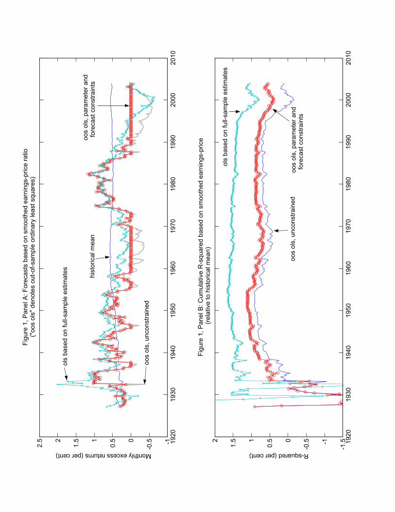
1920

1930

1940

1950

1960

1970

1980

1990

2000

2010

-1

-0.50

0.51

1.52

2.5

Figu

re 1

, Pan

el A

: For

ecas

ts b

ased

on

smoo

thed

ear

ning

s-pr

ice

ratio

("oo

s ol

s" d

enot

es o

ut-o

f-sam

ple

ordi

nary

leas

t squ

ares

)

Monthly excess returns (per cent)

1920

1930

1940

1950

1960

1970

1980

1990

2000

2010

-1.5-1

-0.50

0.51

1.52

Figu

re 1

, Pan

el B

: Cum

ulat

ive

R-s

quar

ed b

ased

on

smoo

thed

ear

ning

s-pr

ice

(rel

ativ

e to

his

toric

al m

ean)

R-squared (per cent)

oos

ols,

unc

onst

rain

ed

oos

ols,

par

amet

er a

ndfo

reca

st c

onst

rain

ts

hist

oric

al m

ean

ols

base

d on

full-

sam

ple

estim

ates

oos

ols,

unc

onst

rain

ed

oos

ols,

par

amet

er a

ndfo

reca

st c

onst

rain

ts

ols

base

d on

full-

sam

ple

estim

ates