Embed Size (px)
Citation preview
NBER WORKING PAPER SERIES
PRODUCTS AND PRODUCTIVITY
Peter K. SchottAndrew B. BernardStephen J. Redding
Working Paper 11575http://www.nber.org/papers/w11575
NATIONAL BUREAU OF ECONOMIC RESEARCH1050 Massachusetts Avenue
Cambridge, MA 02138August 2005
Bernard and Schott acknowledge financial support from the National Science Foundation (SES-0241474).Redding acknowledges financial support from a Philip Leverhulme Prize. Responsibility for any opinionsand errors lies with the authors. The views expressed herein are those of the author(s) and do not necessarilyreflect the views of the National Bureau of Economic Research.
©2005 by Peter K. Schott, Andrew B. Bernard and Stepehn J. Redding. All rights reserved. Shortsections of text, not to exceed two paragraphs, may be quoted without explicit permission provided thatfull credit, including © notice, is given to the source.

Products and Productivity Peter K. Schott, Andrew B. Bernard and Stephen J. ReddingNBER Working Paper No. 11575August 2005JEL No. L11, D21, L60
ABSTRACT
Firms' decisions about which goods to produce are often made at a more disaggregate level than the
data observed by empirical researchers. When products differ according to production technique or
the way in which they enter demand, this data aggregation problem introduces a bias into standard
measures of firm productivity. We develop a theoretical model of heterogeneous firms endogenously
self-selecting into heterogeneous products. We characterize the bias introduced by unobserved
variation in product mix across firms, and the implications of this bias for identifying firm and
industry responses to exogenous policy shocks such as deregulation. More generally, we demonstrate
that product switching gives rise to a richer set of industry-level dynamics than models where firm
product mix remains fixed.
Andrew B. BernardTuck School of Business AdministrationDartmouth College100 Tuck HallHanover, NH 03755and [email protected]
Stephen ReddingLondon School of EconomicsHoughton StreetLondon WC2A 2AEUNITED [email protected]
Peter K. SchottYale School of Management135 Prospect StreetNew Haven, CT 06520-8200and [email protected]
Products and Productivity 2
1. Introduction
Product choice is one of the central business decisions made by a firm. Apple’sdecision to enter the market for personal music players with the iPod was a substantivedeparture from its existing product mix and has received much attention.1 Whilecentral to business strategy, firms’ decisions about which product markets to enter areoften made at a more disaggregate level than the data available to researchers. Thismismatch is important for the measurement of productivity because the products thatfirms switch into may utilize different production techniques — and display differentconsumer demand patterns — than the products firms leave behind. As a result,variation in firms’ observed performance may be driven by unobserved product choicesin addition to underlying (and observable) firm characteristics.This paper examines the implications of unobserved product-mix variation and
product switching for the measurement of firm- and industry-level productivity. Wedevelop a general equilibrium model of industry evolution where heterogeneous firmsendogenously self-select into asymmetric products within an industry. We demon-strate that production-technology differences across products and product-choice vari-ation across firms interact to bias standard superlative-index and production-function-based estimates of firm productivity. This bias persists even if the econometrician canobserve and control for firm-specific variation in prices, inputs and output. Solvingthe problem requires knowledge of the evolution of firms’ product mix over time.We demonstrate that measured productivity differences across firms can be decom-
posed into a component due to true differences in firm productivity and a componentattributable to variation in production technology across products. Depending onhow product technologies vary, measured productivity dispersion can exceed or fallshort of true productivity variation. This finding suggests that differences in firms’product mix may play a role in explaining the substantial within-industry variationin firm productivity noted in many empirical studies.2 At the industry level, weshow that measured productivity depends upon the weight of products in consumerutility. Changes in these weights cause estimated productivity to rise or fall even iftrue industry productivity remains the same.Our approach emphasizes the role of product choice by surviving firms — along
with ongoing entry and exit of firms — in mediating firm and industry responses toexogenous shifts in public policy such as deregulation. We show that estimates of
1See, for example, ‘The Meaning of iPod’, The Economist, June 10th, 2004.2See, for example, the survey in Foster et al. (2001).
Products and Productivity 3
these responses are biased in the presence of unobserved product switching. Eventhough true firm productivity is a parameter in the model and remains unchangedduring deregulation, firms may appear as if they are experiencing productivity growthdue to their endogenous decisions to switch products. For this reason, identification offirm productivity growth as a result of policy reforms is incomplete unless informationon the goods firms produce before and after the reform is incorporated into theanalysis. More generally, we demonstrate that product switching gives rise to aricher set of industry-level dynamics than models where firm product mix remainsfixed. In the framework we develop, deregulation generates aggregate (i.e., industry-level) productivity growth through three channels: the exit of low productivity firms,changes in the composition of output across firms that keep making the same product,and changes in the relative importance of different product markets within the sameindustry. Accounting for these responses promotes more comprehensive evaluationsof public policy.Our findings contribute to a wide range of research in the international trade,
productivity and macroeconomic growth literatures. A great deal of empirical workin these fields has made use of plant- and firm-level datasets from production censusesor surveys. These micro datasets have yielded many insights and are a considerableimprovement over the industry-level datasets that preceded them.3 Nevertheless,most studies making use of microdata assign firms (or plants) to a single, relatively-aggregate industry despite variation in firms’ underlying product mix.4 In the U.S.manufacturing census, for example, BMW would be allocated to the four-digit Stan-dard Industry Classification (SIC) 3711 “Motor Vehicles and Car Bodies” based onthe company’s main source of revenue, which is manufacturing passenger cars. Butpassenger cars are only one five-digit product within this four-digit industry. Firmsproducing buses, combat vehicles, tractors and a variety of truck categories would alsobe found in SIC 3711.5 As a result, estimation of BMW’s productivity might involve
3Early studies using microdata include Davis and Haltiwanger (1991) and Baily et al. (1992).4Exceptions are where detailed information on the product market is used, as for example in
Berry et al. (1995), Goldberg (1995) and Syverson (2004).5Similarly, the UK four-digit industry called Manufacture of Motor Vehicles (UKSIC03
3410) includes passenger cars, buses, commercial vehicle and golf carts among others. Seehttp://www.statistics.gov.uk/methods_quality/sic/downloads/UK_SIC_Vol1(2003).pdf. Sincethe UK system is designed to comply with Eurostat regulations on the common statistical classifi-cation of economic activities (NACE), other European classification schemes face similar problemsof clustering dissimilar products within an industry. While attempts have been made to reviseindustrial classifications to group products and industries by production processes, it remains in-evitable that activities with heterogeneous production techniques and demand-side characteristicsare classified together.

Products and Productivity 4
grouping it with defense contractors such as AM General which produces armor-plated Humvees. The likely dissimilarity of production technologies and demandpatterns across products as diverse as passenger cars and combat vehicles highlightsthe difficulties of using coarse industry classifications to identify firm productivity.There is a long tradition in the industrial organization literature of analyzing en-
dogenous product choice, including Hotelling (1929), Lancaster (1966), Shaked andSutton (1982), Spence (1976) and Sutton (1998) among others. More recent researchby Berry et al. (1995), Hausman (1997), Petrin (2002) and Trajtenberg (1989) hassought to quantify the welfare gains from new product introduction. Other work hasemphasized problems of measuring productivity using revenue data when firms oper-ate in imperfectly competitive markets and charge different prices, including Kletteand Griliches (1996), Levinsohn and Melitz (2002), Katayama, Lu and Tybout (2003),De Loecker (2005) and Martin (2005).A separate tradition has analyzed industry dynamics, where the Darwinian se-
lection of high productivity firms through entry and exit is central in determiningindustry equilibrium, as in Jovanovic (1982), Hopenhayn (1992) and Ericsson andPakes (1995). In contrast with the research noted above, product choice does notfeature prominently in this literature, where the decision to create a firm is equivalentto the decision to enter a product market. One explanation for this difference maybe that models of industry dynamics solve for heterogeneous quantities and pricesacross firms and trace the stochastic evolution of the firm productivity distribution.Analyzing the dynamics of entire distributions in general equilibrium is a demandingexercise. To allow heterogeneous firms to choose between products with diverse at-tributes would be to introduce a further equilibrium distribution (the distribution ofproducts across firms) that must be analyzed over time.We make progress in this direction by adopting a number of stark assumptions.
In particular, we build on Melitz’s (2003) model of industry equilibrium, which sub-stantially simplifies industry dynamics by assuming a monopolistically competitiveindustry structure where firms produce varieties of a single product, and by assumingthat firm productivity is a parameter which is drawn from a fixed distribution at thepoint of entry, with firms facing a constant exogenous probability of death thereafter.Into this structure we introduce a choice between two heterogeneous products withdifferent production techniques. These products enter demand asymmetrically, andtheir relative price is determined endogenously in general equilibrium. We believethis to be the simplest framework for understanding the impact of product choice onproductivity measurement. It captures both product heterogeneity and self-selection
Products and Productivity 5
by firms into product markets while yielding particularly tractable results.The remainder of the paper is structured as follows. Section 2 places the paper
in the context of the existing literature on deregulation, industry dynamics and pro-ductivity. Section 3 develops the theoretical model. Section 4 solves for industryequilibrium. Section 5 examines the properties of general equilibrium and derivesthe bias in standard productivity measures. Section 6 examines the implications ofan exogenous policy reform, in the form of a reduction in barriers to entry, on prod-uct choice, measured productivity growth at the firm-level and on aggregate industryproductivity growth. Section 7 concludes. An appendix at the end of the papercollects together proofs and technical derivations.
2. Deregulation, Industry Dynamics and Productivity
A great deal of recent research in industrial organization and international tradefocuses on industry responses to deregulation and trade liberalization. The influen-tial study of the U.S. telecommunications industry by Olley and Pakes (1996) andthe analyses of trade liberalization in Chile by Tybout et al. (1991) and Pavcnik(2002) are prominent examples. An important contribution of this analysis is thedevelopment of methodologies for consistent estimation of productivity when firmsendogenously choose factor inputs as well as whether or not to exit the industryin response to changing market conditions and technology.6 The estimated valuesof productivity that emerge from this literature show considerable dispersion acrossplants and firms within narrowly defined industries as well as exit by low productivityfirms. Changes in the composition of output are found to play an important role inthe response of industries to exogenous changes in the policy environment. Pavcnik(2002), for example, finds that aggregate productivity growth in Chile grew by 19.3percent during the seven years following trade liberalization in 1979, with a contribu-tion of 6.6 percent from increased productivity within plants and a 12.7 percent fromthe reallocation of resources from less to more efficient producers.A related literature has argued that gross rates of firm entry and exit are large
relative to net rates, and that firm entry and exit play an important role in accountingfor aggregate productivity growth. Leading examples include Baily et al. (1992),Davis and Haltiwanger (1991), Dunne et al. (1989), Disney et al. (2003) and Foster etal. (2002). Foster et al. (2002), for example, find that virtually all of the productivitygrowth in the U.S. retail trade sector during the 1990s is accounted for by more
6See in particular Olley and Pakes (1996) and Levinsohn and Petrin (2003).
Products and Productivity 6
productive entrants displacing less productive exiters.Finally, a separate body of research has emphasized the problems associated with
measuring productivity using revenue data when there is dispersion in output pricesacross firms within industries, including work by Klette and Griliches (1996), Levin-sohn and Melitz (2002), Katayama et al. (2003), De Loecker (2005), and Martin(2005). In the presence of this price dispersion, deflating firm revenue using a com-mon industry price deflator, as is common in empirical work, yields biased estimatesof firm productivity.The theoretical model we develop in this paper incorporates all of these features:
heterogeneous firm productivity, ongoing entry and exit in steady-state, selectionon survival where exiting firms are on average of lower productivity, and imperfectcompetition inducing variation in prices across firms. In addition, we incorporatean additional feature of firm-level data not emphasized in existing research, namelythe idea that firm choices about which good to manufacture are typically made ata more disaggregate level than the industry concordances according to which firmsare classified. These products often have different production technologies and dis-play heterogeneous consumer demand patterns, which mean that they are not wellmodelled as differentiated varieties of the same product. Even if firm-specific dataon prices or information on physical quantities of output is available, measured firmproductivity is biased because it captures both true productivity differences acrossfirms as well as differences across products in production technique.We illustrate the importance of these ideas by describing a particular micro
dataset, the Longitudinal Research Database (LRD) of the U.S. Census Bureau. Inthe LRD, manufacturing censuses are conducted every five years. Plants are allo-cated to four-digit SIC industries, of which there are 457, according to the industrythat accounts for the main share of plant revenue. Information on output and inputssuch as employment, wages, physical capital, materials, and energy is reported at theplant-level.Existing research relying on the LRD generally focuses on plants’ primary indus-
tries.7 However, more detailed information on plant production is available. TheLRD also tracks the identity and output of plants’ five-digit SIC products, of whichthere are 1462. To provide a sense of the relative level of detail between productsand industries, Table 1 lists the thirteen products captured by industry 3357, “Non-ferrous Wire-Drawing and Insulating.” The products in this industry — which rangefrom Copper Wire (33571) to Fiber Optic Cable (33579) — differ both in terms of end
7See, for example, Baily et al. (1992), Davis and Haltiwanger (1991) and Olley and Pakes (1996).
Products and Productivity 7
use and in terms of the inputs and technologies required to manufacture them. Thecurrent UK SIC2003 system also groups fiber optic and insulated wire cable underthe four-digit industry 3130, Manufacture of Insulated Wire and Cable.8
Table 2 provides a more systematic view of the level of product detail availablein the U.S. SIC by reporting the number of four- and five-digit categories in eachtwo-digit sector. The typical two-digit manufacturing sector has 24 industries and76 products. However, there is a substantial degree of variation across sectors. Thenumber of five-digit products per two-digit sector ranges from a low of 12 in Leather(31) to 187 in Industrial Machinery (35). Similarly, the number of five-digit productsper four-digit industry ranges from a low of 1.1 in Leather to a high of 5.1 in Printingand Publishing (27). The industry highlighted in Table 1, Nonferrous Wiredrawingand Insulating (3357), is just one of 26 Primary Metal industries, and its productsrepresent 14 percent (13/89) of the total number of products in that sector.In the theoretical model developed below, we allow heterogeneous firms to endoge-
nously self-select into products that vary in terms of their demand and supply-sideattributes. Product choice is shaped by the interaction of the heterogeneous charac-teristics of firms and products. The product chosen by the firm affects its measuredproductivity and its response to industry deregulation. The distribution of firmsacross products influences measured industry productivity at a point in time. Theendogenous re-sorting of firms across products in response to industry deregulationshapes the dynamic response of the industry as a whole to policy reform over time.
3. Theoretical Model
Consider a single industry within which consumers and firms choose whether toconsume and produce varieties of two distinct products.9 To keep the analysis astractable as possible, we assume that consumer preferences between the two products
8Even at further levels of disaggregation, e.g. seven-digit SIC categories, goods are often quitedistinct. For example, in the Motor Vehicles Parts and Accessories industry (3714), the five-digitproduct “Gasoline Engines and Gasoline Engine Parts for Motor Vehicles, New” (37142) includes thefollowing seven-digit categories: “Intake Manifolds” (3714206), “Rocker Arms and Parts (3714215),“Fuel Injection Systems” (3714218), and “Radiators, Complete” (3714235). These seven-digitcategories are likely to display heterogeneous technological requirements and to face different patternsof consumer demand. For a complete list of four-, five-, and seven- digit SIC87 categories, see U.S.Census (1996) available at http://www.census.gov/prod/2/manmin/mc92-r-1.pdf.
9It is straightforward to embed this framework in a multi-industry model or to allow a finitenumber of distinct products within the industry. The model developed here is the simplest frame-work within which to demonstrate the importance of firms’ choice between heterogeneous productsin influencing measured firm and industry outcomes.
Products and Productivity 8
can be well represented with the following CES utility function:
U = [aCν1 + (1− a)Cν
2 ]1/ν . (1)
where a captures the relative strength of preferences for each product, and we assumethat the products are imperfect substitutes with elasticity of substitution ψ = 1
1−ν >
1. Firms produce horizontally differentiated varieties of their chosen product. Ci istherefore a consumption index defined over varieties ω of each product i:
Ci =
∙Zω∈Ωi
qi(ω)ρdω
¸1/ρ, Pi =
∙Zω∈Ωi
pi(ω)1−σdω
¸1/1−σ. (2)
where Ωi is the set of available varieties in market i, Pi is the price index dual toCi, and σ = 1
1−ρ > 1 is the elasticity of substitution between varieties of the sameproduct. We make the natural assumption that varieties of the same product aremore easily substitutable than different products, so that σ > ψ.Consumer expenditure minimization yields the following expression for equilib-
rium expenditure (equals revenue, ri(ω)) on a variety:
ri(ω) = Ri
µpi(ω)
Pi
¶1−σ= αi (P)R
µpi(ω)
Pi
¶1−σ(3)
which is increasing in aggregate expenditure (equals aggregate revenueR = R1+R2 =Rω∈Ω1 r1(ω)dω +
Rω∈Ω2 r2(ω)dω), increasing in the share of expenditure allocated to
product i, αi(P2/P1) = αi(P), decreasing in own variety price, pi(ω), and increasingin the price of competing varieties as summarized in the price index, Pi.With CES utility, the share of expenditure allocated to product 1 is increasing
in the relative price of product 2, P = P2/P1 (since ψ > 1), and increasing in therelative weight given to product 1 in consumer utility, a:
α1 (P) ="1 +
µ1− a
a
¶ψ
P1−ψ#−1
, α2 (P) = 1− α1 (P) . (4)
3.1. Production
As well as entering demand in different ways, the products have different produc-tion technologies. We consider the case where this difference in production technologytakes the form of a difference in the fixed and variable costs of production. We as-sume that product 2 has a higher fixed cost of production: f2 > f1. Variable costsare indexed by the parameter bi and, without loss of generality, we normalize b1 = 1
Products and Productivity 9
and b2 = b. We allow variable costs of production for product 2 to be either smalleror greater than those for product 1.Labor is the sole factor of production and is supplied inelastically at its aggregate
level L , which also indexes the size of the economy. The production technologyfollows Melitz (2003) in that variable cost is assumed to depend on heterogeneousfirm productivity. We differ in that we allow for multiple distinct products andhence endogenous product choice within the industry. The labor required to produceqi units of a variety in product market i is given by:
li = fi +biqiϕ
(5)
so that the variable cost of production depends on bi, which is common to all firms,as well as on the firm-specific productivity, ϕ.10
The existence of fixed production costs implies that, in equilibrium, each firm willchoose to produce a unique variety. Profit maximization yields the standard resultthat equilibrium prices are a constant mark-up over marginal cost, with the size ofthe mark-up depending on the elasticity of substitution between varieties:
pi(ϕ) =
µσ
σ − 1
¶wbiϕ
. (6)
We choose the wage as the numeraire so that w = 1. Using this choice ofnumeraire and the pricing rule in the expression for revenue above, equilibrium firmrevenue and profits are:
ri(ϕ) = αi(P)RµPiρ
ϕ
bi
¶σ−1(7)
πi(ϕ) =ri(ϕ)
σ− fi.
One property of equilibrium revenue that will prove useful below is that the relativerevenue of two firms with different productivity levels in the same product marketdepends solely on their relative productivity: ri (ϕ00) = (ϕ00/ϕ0)
σ−1 ri (ϕ0). Similarly,
the relative revenue of two firms with different productivity levels in different productmarkets depends on their relative productivities, the relative variable cost of making
10The assumption that fixed costs of production are independent of productivity captures the ideathat many fixed costs, such as building and equipping a factory with machinery, are unlikely to varysubstantially with firm productivity. As long as fixed costs are less sensitive to productivity thanvariable costs, there will be endogenous selection on productivity in firms’ exit and product choicedecisions.

Products and Productivity 10
the two products, the relative expenditure share devoted to the two products, andrelative price indices:
r2 (ϕ00) =
µ1− α1(P)α1(P)
¶ ∙µϕ00
ϕ0
¶P 1b
¸σ−1r1 (ϕ
0) . (8)
3.2. Industry Entry and Exit
To enter the industry (and produce either product), firms must pay a fixed entrycost, fe > 0, which is thereafter sunk. After paying the sunk cost, firms draw theirproductivity, ϕ, from a distribution, g (ϕ), with corresponding cumulative distributionG (ϕ). This formulation captures the idea that there are sunk costs of entering anindustry and that, once these costs are incurred, some uncertainty regarding thenature of production and firm profitability is realized. Firm productivity is assumedto remain fixed thereafter, and firms face a constant exogenous probability of death,δ, which we interpret as due to force majeure events beyond managers’ control.11
A particularly tractable productivity distribution, which we use at some pointsbelow and which provides a good approximation to observed firm-level productivitydata is the Pareto distribution, g (ϕ) = zkzϕ−(z+1). The parameter k > 0 correspondsto the minimum value of productivity in the industry, while z > 0 determines theskewness of the distribution, and in order for the variance of log firm sales to be finitewe require z > σ − 1.After entry, firms decide whether to begin producing in the industry or exit. If
they decide to produce, they choose which product to make. The value of a firm withproductivity ϕ is, therefore, the maximum of 0 (if the firm exits) or the stream offuture profits from producing one of the two products discounted by the probabilityof firm death:
v (ϕ) = max
½0,1
δπ1 (ϕ) ,
1
δπ2 (ϕ)
¾. (9)
11Firm death ensures steady-state entry into the industry. New entrants make an endogenous exitdecision, since their decision whether or not to produce in the industry depends on their productivitydraw ϕ from the distribution g (ϕ). Together with fixed production costs, this will generate the resultthat exiting firms are on average less productive than surviving firms. For incumbent firms, theprobability of death δ is independent of productivity. This assumption can be relaxed by allowingfirm productivity to evolve stochastically after entry (e.g. Hopenhayn 1992). While this wouldachieve greater realism, it would not change the qualitative results below on the importance ofendogenous product choice for measured firm and industry productivity, and would come at the costof a substantial increase in the complexity of the industry dynamics.
Products and Productivity 11
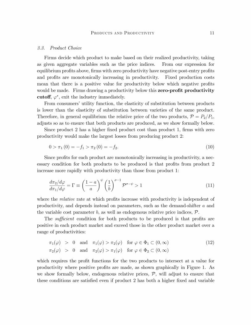
3.3. Product Choice
Firms decide which product to make based on their realized productivity, takingas given aggregate variables such as the price indices. From our expression forequilibrium profits above, firms with zero productivity have negative post-entry profitsand profits are monotonically increasing in productivity. Fixed production costsmean that there is a positive value for productivity below which negative profitswould be made. Firms drawing a productivity below this zero-profit productivitycutoff, ϕ∗, exit the industry immediately.From consumers’ utility function, the elasticity of substitution between products
is lower than the elasticity of substitution between varieties of the same product.Therefore, in general equilibrium the relative price of the two products, P = P2/P1,adjusts so as to ensure that both products are produced, as we show formally below.Since product 2 has a higher fixed product cost than product 1, firms with zero
productivity would make the largest losses from producing product 2:
0 > π1 (0) = −f1 > π2 (0) = −f2. (10)
Since profits for each product are monotonically increasing in productivity, a nec-essary condition for both products to be produced is that profits from product 2increase more rapidly with productivity than those from product 1:
dπ2/dϕ
dπ1/dϕ= Γ ≡
µ1− a
a
¶ψ µ1
b
¶σ−1Pσ−ψ > 1 (11)
where the relative rate at which profits increase with productivity is independent ofproductivity, and depends instead on parameters, such as the demand-shifter a andthe variable cost parameter b, as well as endogenous relative price indices, P.The sufficient condition for both products to be produced is that profits are
positive in each product market and exceed those in the other product market over arange of productivities:
π1(ϕ) > 0 and π1(ϕ) > π2(ϕ) for ϕ ∈ Φ1 ⊂ (0,∞) (12)
π2(ϕ) > 0 and π2(ϕ) > π1(ϕ) for ϕ ∈ Φ2 ⊂ (0,∞)
which requires the profit functions for the two products to intersect at a value forproductivity where positive profits are made, as shown graphically in Figure 1. Aswe show formally below, endogenous relative prices, P, will adjust to ensure thatthese conditions are satisfied even if product 2 has both a higher fixed and variable
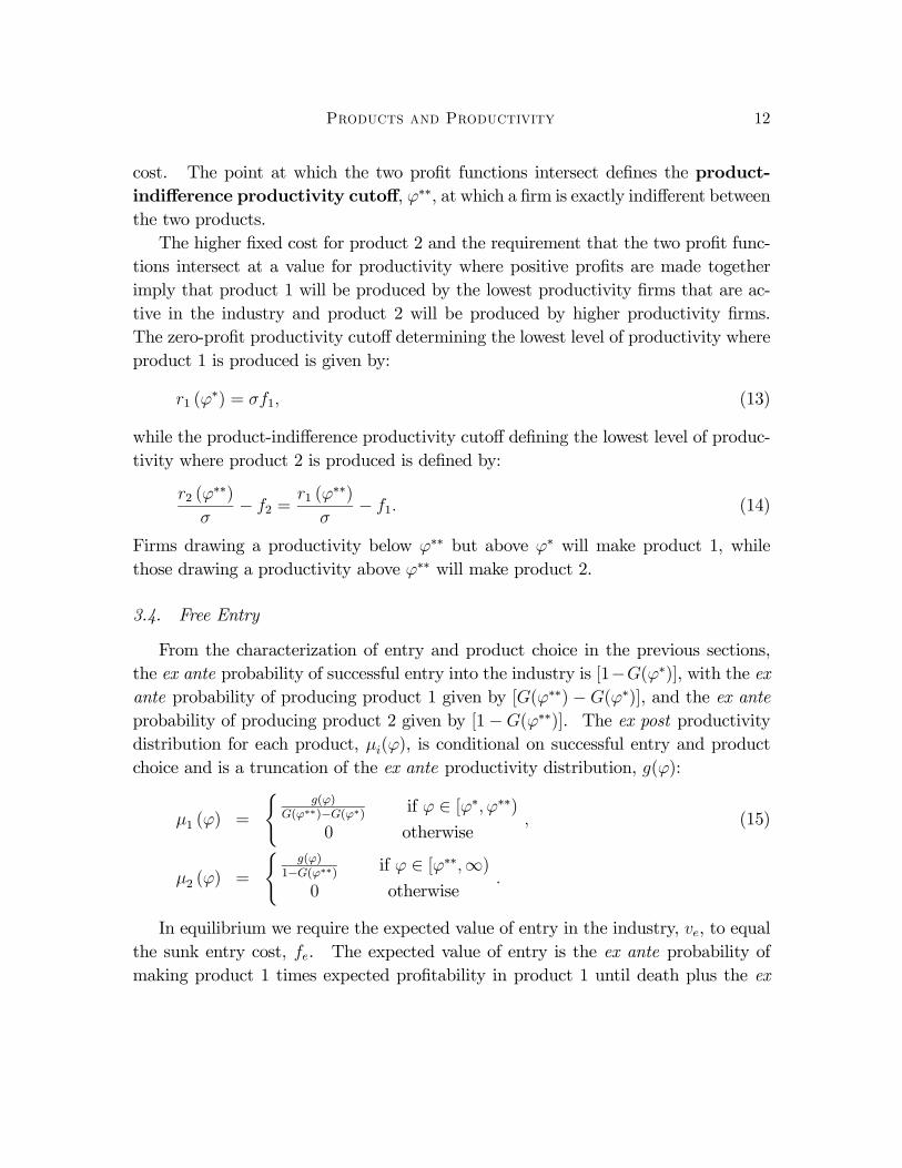
Products and Productivity 12
cost. The point at which the two profit functions intersect defines the product-indifference productivity cutoff, ϕ∗∗, at which a firm is exactly indifferent betweenthe two products.The higher fixed cost for product 2 and the requirement that the two profit func-
tions intersect at a value for productivity where positive profits are made togetherimply that product 1 will be produced by the lowest productivity firms that are ac-tive in the industry and product 2 will be produced by higher productivity firms.The zero-profit productivity cutoff determining the lowest level of productivity whereproduct 1 is produced is given by:
r1 (ϕ∗) = σf1, (13)
while the product-indifference productivity cutoff defining the lowest level of produc-tivity where product 2 is produced is defined by:
r2 (ϕ∗∗)
σ− f2 =
r1 (ϕ∗∗)
σ− f1. (14)
Firms drawing a productivity below ϕ∗∗ but above ϕ∗ will make product 1, whilethose drawing a productivity above ϕ∗∗ will make product 2.
3.4. Free Entry
From the characterization of entry and product choice in the previous sections,the ex ante probability of successful entry into the industry is [1−G(ϕ∗)], with the exante probability of producing product 1 given by [G(ϕ∗∗)−G(ϕ∗)], and the ex anteprobability of producing product 2 given by [1−G(ϕ∗∗)]. The ex post productivitydistribution for each product, µi(ϕ), is conditional on successful entry and productchoice and is a truncation of the ex ante productivity distribution, g(ϕ):
µ1 (ϕ) =
(g(ϕ)
G(ϕ∗∗)−G(ϕ∗) if ϕ ∈ [ϕ∗, ϕ∗∗)0 otherwise
, (15)
µ2 (ϕ) =
(g(ϕ)
1−G(ϕ∗∗) if ϕ ∈ [ϕ∗∗,∞)0 otherwise
.
In equilibrium we require the expected value of entry in the industry, ve, to equalthe sunk entry cost, fe. The expected value of entry is the ex ante probability ofmaking product 1 times expected profitability in product 1 until death plus the ex
Products and Productivity 13
ante probability of making product 2 times expected profitability in product 2 untildeath, and the free entry condition is:
ve =
∙G (ϕ∗∗)−G (ϕ∗)
δ
¸π1 +
∙1−G (ϕ∗∗)
δ
¸π2 = fe, (16)
where πi is expected or average firm profitability in product market i. Equilibriumrevenue and profit in each market are constant elasticity functions of firm productivity(equation (7)) and, therefore, average revenue and profit are equal respectively tothe revenue and profit of a firm with weighted average productivity, ri = ri(eϕi)
and πi = πi(eϕi), where weighted average productivity, ϕ1(ϕ∗, ϕ∗∗) and ϕ2(ϕ
∗∗), isdetermined by the ex post productivity distributions, µi (ϕ), and is defined formallyin the Appendix.
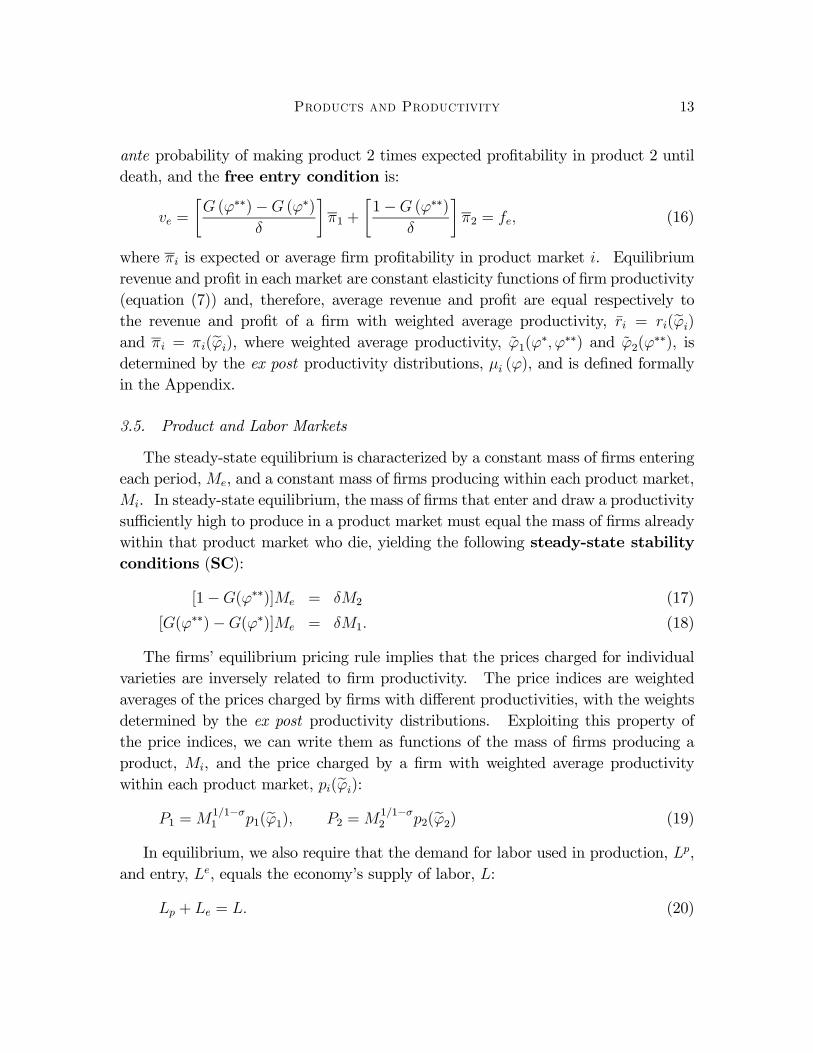
3.5. Product and Labor Markets
The steady-state equilibrium is characterized by a constant mass of firms enteringeach period,Me, and a constant mass of firms producing within each product market,Mi. In steady-state equilibrium, the mass of firms that enter and draw a productivitysufficiently high to produce in a product market must equal the mass of firms alreadywithin that product market who die, yielding the following steady-state stabilityconditions (SC):
[1−G(ϕ∗∗)]Me = δM2 (17)
[G(ϕ∗∗)−G(ϕ∗)]Me = δM1. (18)
The firms’ equilibrium pricing rule implies that the prices charged for individualvarieties are inversely related to firm productivity. The price indices are weightedaverages of the prices charged by firms with different productivities, with the weightsdetermined by the ex post productivity distributions. Exploiting this property ofthe price indices, we can write them as functions of the mass of firms producing aproduct, Mi, and the price charged by a firm with weighted average productivitywithin each product market, pi(eϕi):
P1 =M1/1−σ1 p1(eϕ1), P2 =M
1/1−σ2 p2(eϕ2) (19)
In equilibrium, we also require that the demand for labor used in production, Lp,and entry, Le, equals the economy’s supply of labor, L:
Lp + Le = L. (20)
Products and Productivity 14
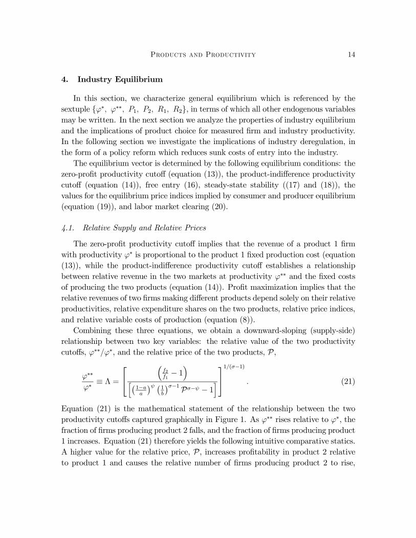
4. Industry Equilibrium
In this section, we characterize general equilibrium which is referenced by thesextuple ϕ∗, ϕ∗∗, P1, P2, R1, R2, in terms of which all other endogenous variablesmay be written. In the next section we analyze the properties of industry equilibriumand the implications of product choice for measured firm and industry productivity.In the following section we investigate the implications of industry deregulation, inthe form of a policy reform which reduces sunk costs of entry into the industry.The equilibrium vector is determined by the following equilibrium conditions: the
zero-profit productivity cutoff (equation (13)), the product-indifference productivitycutoff (equation (14)), free entry (16), steady-state stability ((17) and (18)), thevalues for the equilibrium price indices implied by consumer and producer equilibrium(equation (19)), and labor market clearing (20).
4.1. Relative Supply and Relative Prices
The zero-profit productivity cutoff implies that the revenue of a product 1 firmwith productivity ϕ∗ is proportional to the product 1 fixed production cost (equation(13)), while the product-indifference productivity cutoff establishes a relationshipbetween relative revenue in the two markets at productivity ϕ∗∗ and the fixed costsof producing the two products (equation (14)). Profit maximization implies that therelative revenues of two firms making different products depend solely on their relativeproductivities, relative expenditure shares on the two products, relative price indices,and relative variable costs of production (equation (8)).Combining these three equations, we obtain a downward-sloping (supply-side)
relationship between two key variables: the relative value of the two productivitycutoffs, ϕ∗∗/ϕ∗, and the relative price of the two products, P,
ϕ∗∗
ϕ∗≡ Λ =
⎡⎣³f2f1− 1´
h¡1−aa
¢ψ ¡1b
¢σ−1Pσ−ψ − 1i⎤⎦1/(σ−1) . (21)
Equation (21) is the mathematical statement of the relationship between the twoproductivity cutoffs captured graphically in Figure 1. As ϕ∗∗ rises relative to ϕ∗, thefraction of firms producing product 2 falls, and the fraction of firms producing product1 increases. Equation (21) therefore yields the following intuitive comparative statics.A higher value for the relative price, P, increases profitability in product 2 relativeto product 1 and causes the relative number of firms producing product 2 to rise,
Products and Productivity 15
i.e. a reduction in ϕ∗∗ relative to ϕ∗, since σ > ψ. For a given value for the relativeprice, P, a higher fixed cost for product 2 , f2, reduces profitability in product 2 andcauses the relative number of firms producing product 2 to fall, i.e. an increase inϕ∗∗ relative to ϕ∗.
4.2. Relative Demand and Relative Prices
The expressions for the two price indices yield an equation for relative prices asa function of the relative mass of firms and the relative price charged by a firm withweighted average productivity in each product market (equation (19)). The twosteady-state stability conditions yield an equation for the relative mass of firms as afunction of the two productivity cutoffs (equations (17) and (18)).Combining these expressions yields an upward-sloping demand-side relationship
between the relative value of the two productivity cutoffs and the relative price of thetwo products:
Ψ
µϕ∗∗
ϕ∗
¶≡"bσ−1
R ϕ∗∗ϕ∗ ϕσ−1g (ϕ) dϕR∞
ϕ∗∗ ϕσ−1g (ϕ) dϕ
#= Pσ−1. (22)
An increase in the relative consumer price index for product 2, P, reduces demandfor product 2 relative to product 1 and shrinks the range of productivities whereproduct 2 is produced relative to the range where product 1 is produced, i.e. anincrease in ϕ∗∗/ϕ∗. For a given value of ϕ∗∗/ϕ∗, an increase in b, the relative variablecost for product 2, raises the price of product 2 varieties relative to product 1 varieties,i.e. an increase in P.
4.3. Free Entry
The free entry condition can be written in a more convenient form using the ex-pression for the zero-profit productivity cutoff, the relationship between the revenuesof firms producing varieties in the same market with different productivities, and thesupply-side relationship between the two productivity cutoffs derived above. Com-bining equation (13), ri (ϕ00) = (ϕ00/ϕ0)
σ−1 ri (ϕ0), and equation (21), we can write the
free entry condition as:
Products and Productivity 16
ve =f1δ
Z Λϕ∗
ϕ∗
"µϕ
ϕ∗
¶σ−1− 1#g(ϕ)dϕ (23)
+f1δ
Z ∞
Λϕ∗
"µ1− a
a
¶ψ µ1
b
¶σ−1Pσ−ψ
µϕ
ϕ∗
¶σ−1− f2
f1
#g(ϕ)dϕ = fe.
where Λ is defined in equation (21).This way of writing the free entry condition clarifies the relationship between the
sunk cost of entry and the zero-profit productivity cutoff. An increase in the sunkentry cost, fe, requires an increase in the expected value of entry, ve. Since theexpected value of entry above is monotonically decreasing in ϕ∗, this requires a fall inthe zero-profit productivity cutoff. Intuitively, the higher sunk cost of entering theindustry reduces the mass of entrants, which increases ex post profitability, enablinglower productivity firms to cover their fixed production costs and survive in theindustry.
4.4. Steady-state Stability, Labor Market Clearing and Goods Market Clearing
Using the steady-state stability conditions to substitute for the ex ante probabilityof producing each product in the free entry condition, total payments to labor usedin entry equal total industry profits: Le = Mefe = M1π1 +M2π2 = Π (by choice ofnumeraire, w = 1). The existence of a competitive fringe of potential entrants meansthat firms enter until the expected value of entry equals the sunk entry cost, and asa result the entire value of industry profits is paid to labor used in entry.Total payments to labor used in production equal the difference between industry
revenue, R, and industry profits, Π: Lp = R−Π. Taking these two results together,total payments to labor used in both entry and production equal industry revenue,L = R. Substituting for R in the expressions for Le and Lp above, this establishesthat the labor market clears.In equilibrium we also require the goods market to clear, which implies that the
value of expenditure equals the value of revenue for each product. Utility max-imization implies that the consumer allocates the expenditure shares α1 (P) and(1− α1 (P)) to the two products. Imposing expenditure equals revenue for eachproduct, goods market clearing may be expressed as:
R1 = α1(P)R, R2 = (1− α(P))R. (24)
Products and Productivity 17
4.5. Existence and Uniqueness of Equilibrium
Proposition 1 There exists a unique value of the equilibrium vector ϕ∗ , ϕ∗∗ ,P1,P2, R1, R2. All other endogenous variables of the model may be written as functionsof this equilibrium vector.
Proof. See Appendix
Combining the supply-side relationship between the relative productivity cutoffsand relative prices in equation (21) with the demand-side relationship in equation(22) yields a unique equilibrium value of ϕ∗∗/ϕ∗ and P = P2/P1. In the proof ofProposition 1, we establish that at the unique equilibrium value of P, ϕ∗ > 0 andϕ∗∗ > ϕ∗, so that both products are produced in equilibrium.
5. Properties of Industry Equilibrium
5.1. Endogenous Selection Into Product Markets
Proposition 2 There is non-random selection into product markets, whereby highproductivity firms produce the high fixed cost product.
Proof. See Appendix.
Firms endogenously sort into products based on their heterogeneous character-istics and the diverse attributes of products. As shown in Figure 1 only higherproductivity firms find it profitable to produce the higher fixed cost product. Thevalue for productivity at which the higher fixed cost product is produced dependson the exogenous parameters of the production technology and endogenous relativeprices. Because consumers have a taste for each product, and the elasticity of substi-tution between products is lower than between varieties of the same product, relativeprices adjust so that both products are produced in equilibrium, even if one of theproducts has both a higher fixed and variable cost.With a Pareto productivity distribution, the demand-side relationship between
relative prices and the relative value of the productivity cutoffs in equation (22)simplifies to yield the following expression for relative prices:
P = b [(ϕ∗∗/ϕ∗)γ − 1]1/σ−1 . (25)
Products and Productivity 18
Combining this demand-side relationship with the supply-side relationship be-tween relative prices and the two productivity cutoffs in equation (21), we obtain thefollowing expression for the relative value of the two productivity cutoffs as a functionof parameters alone:∙µ
ϕ∗∗
ϕ∗
¶γ
− 1¸ 1σ−1
=
"µϕ∗∗
ϕ∗
¶1−σ µf2f1− 1¶+ 1
# 1σ−ψ µ
a
1− a
¶ ψσ−ψ
bψ−1σ−ψ . (26)
This expression implicitly defines the equilibrium value of ϕ∗∗/ϕ∗ > 1. In theframework developed here productivity, ϕ, is the heterogeneous firm characteristicand fixed costs, variable costs and the weight of products in demand, fi, bi, a , arethe diverse product attributes that determine the endogenous selection of productsby firms. The effect of each of these parameters on product choice is mediated by theelasticity of substitution between products, ψ, the elasticity of substitution betweenvarieties of each product, σ, and the degree of skewness of the Pareto distribution, γ.Increases in the fixed cost of production for product 2 relative to product 1, f2/f1;increases in the variable cost of production for product 2 relative to product 1, b;and increases in the weight of product 1 in consumer utility, a, increase ϕ∗∗/ϕ∗ andreduce the range of productivities where product 2 is produced.The point that product choice is shaped by the interaction of heterogeneous firm
and product characteristics and results in a non-random distribution of firms acrossproducts is clearly very general. In the remainder of this section, we trace the biasin firm and industry productivity measures that inevitably result unless the empiricalresearcher can observe which products are made by which firms or can combine astructural model of product choice and industry evolution with an observable exoge-nous variable that determines firm product choice but does not affect firm performanceconditional on product choice.
5.2. Product Choice and Firm Productivity
Standard superlative productivity indices (Caves et al. 1982a,b) assume constantreturns to scale and perfect competition to derive a primal measure of productivityfrom the relationship between output and factor inputs or a dual measure of produc-tivity from the relationship between prices and factor costs. With a single factorof production, as in the model developed here, the dual productivity index takes theform:
lnA (ω) = lnw − ln p (ω) (27)
Products and Productivity 19
where A (ω) denotes total factor productivity (TFP) and ω indexes firms. Therefore,a lower value of prices relative to factor costs corresponds to a higher value of TFP.The true relationship between prices, wages and firm productivity in the model is
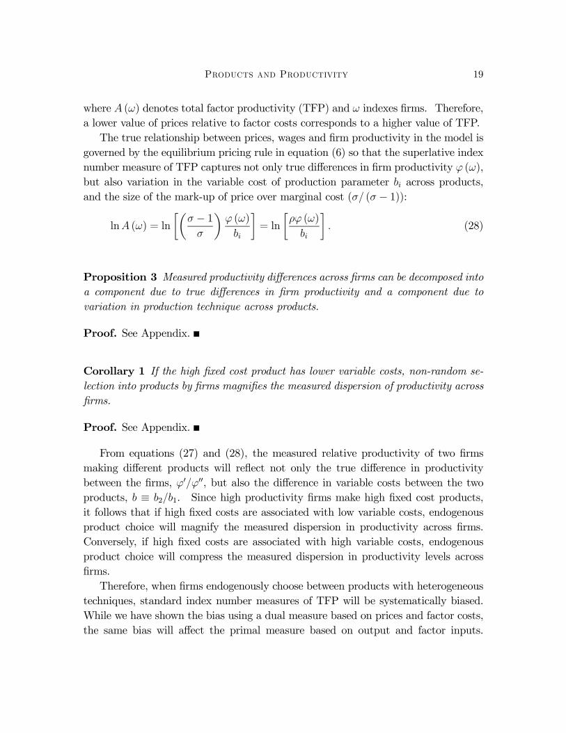
governed by the equilibrium pricing rule in equation (6) so that the superlative indexnumber measure of TFP captures not only true differences in firm productivity ϕ (ω),but also variation in the variable cost of production parameter bi across products,and the size of the mark-up of price over marginal cost (σ/ (σ − 1)):
lnA (ω) = ln
∙µσ − 1σ
¶ϕ (ω)
bi
¸= ln
∙ρϕ (ω)
bi
¸. (28)
Proposition 3 Measured productivity differences across firms can be decomposed intoa component due to true differences in firm productivity and a component due tovariation in production technique across products.
Proof. See Appendix.
Corollary 1 If the high fixed cost product has lower variable costs, non-random se-lection into products by firms magnifies the measured dispersion of productivity acrossfirms.
Proof. See Appendix.
From equations (27) and (28), the measured relative productivity of two firmsmaking different products will reflect not only the true difference in productivitybetween the firms, ϕ0/ϕ00, but also the difference in variable costs between the twoproducts, b ≡ b2/b1. Since high productivity firms make high fixed cost products,it follows that if high fixed costs are associated with low variable costs, endogenousproduct choice will magnify the measured dispersion in productivity across firms.Conversely, if high fixed costs are associated with high variable costs, endogenousproduct choice will compress the measured dispersion in productivity levels acrossfirms.Therefore, when firms endogenously choose between products with heterogeneous
techniques, standard index number measures of TFP will be systematically biased.While we have shown the bias using a dual measure based on prices and factor costs,the same bias will affect the primal measure based on output and factor inputs.
Products and Productivity 20
Though these standard TFP measures are widely used in empirical work, it might beobjected that there are a number of more sophisticated measures of TFP that seek tocontrol for a variety of measurement issues. In particular, it is possible to correct forimperfect competition (Hall 1988, Roeger 1995), increasing returns to scale (Kletteand Griliches 1995), and the absence of firm-specific price data (Klette and Griliches1995, Levinsohn and Melitz 2002, De Loecker (2005) and Martin 2005). Furthermore,rather than measuring productivity using index numbers, a related literature obtainsTFPmeasures from production function estimation (Olley and Pakes 1996, Levinsohnand Petrin 2003).While these techniques control for many sources of measurement error, we now
show that they do not eliminate the bias in productivity measures due to endogenousproduct choice. Measures of imperfect competition control for the size of the mark-up of price over marginal cost. Since to keep the algebra particularly tractable, wehave assumed both products have the same elasticity of demand across varieties, thisadjustment would eliminate the term ((σ − 1) /σ) from measured TFP in equation(28). However, controlling for the size of the mark-up does not eliminate the biasinduced by different products having different production techniques, captured herein the variation in the variable cost of production parameter bi. Furthermore, if weenriched the model to allow different products to have different elasticities of demand,mark-ups would need to be measured at the product level whereas, in much empiricalwork, mark-ups are estimated for the industry as a whole.Second, controlling for increasing returns to scale will not eliminate the bias in
productivity measures. The problem is that the fixed and variable cost parameterswhich determine observed productivity and the degree of increasing returns to scalevary across products. Any productivity measure that does not control for this vari-ation will be biased. Third, the bias does not arise from price deflators only beingavailable at the industry-level and output being measured using revenue rather thanquantity data. The biases we derived above assumed that prices were observed at thefirm-level and we will show in the discussion of production function estimation belowthat primal productivity measures will be systematically biased even if the physicalquantity of output is observed at the firm-level.Fourth, production function estimation will not eliminate the biases in productiv-
ity measures derived here, even assuming that one can control for the simultaneityof firm input choice as in the estimation techniques of Olley and Pakes (1996) andLevinsohn and Petrin (2003). The model implies the following relationship between
Products and Productivity 21
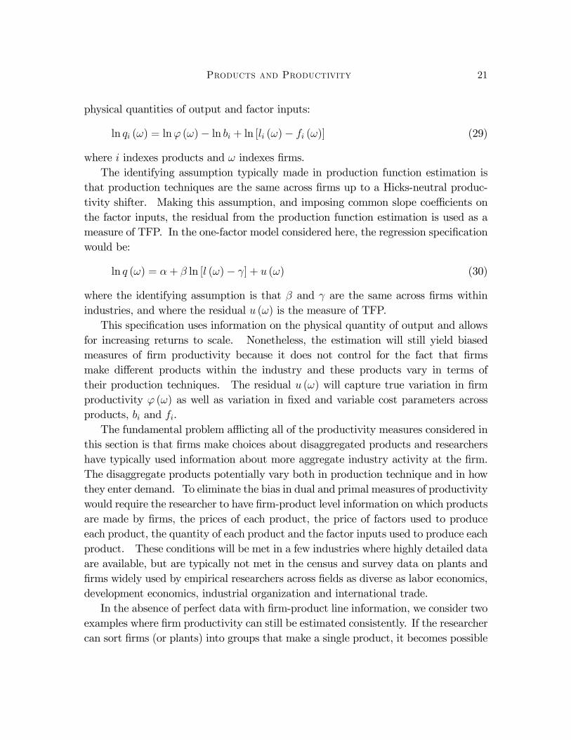
physical quantities of output and factor inputs:
ln qi (ω) = lnϕ (ω)− ln bi + ln [li (ω)− fi (ω)] (29)
where i indexes products and ω indexes firms.The identifying assumption typically made in production function estimation is
that production techniques are the same across firms up to a Hicks-neutral produc-tivity shifter. Making this assumption, and imposing common slope coefficients onthe factor inputs, the residual from the production function estimation is used as ameasure of TFP. In the one-factor model considered here, the regression specificationwould be:
ln q (ω) = α+ β ln [l (ω)− γ] + u (ω) (30)
where the identifying assumption is that β and γ are the same across firms withinindustries, and where the residual u (ω) is the measure of TFP.This specification uses information on the physical quantity of output and allows
for increasing returns to scale. Nonetheless, the estimation will still yield biasedmeasures of firm productivity because it does not control for the fact that firmsmake different products within the industry and these products vary in terms oftheir production techniques. The residual u (ω) will capture true variation in firmproductivity ϕ (ω) as well as variation in fixed and variable cost parameters acrossproducts, bi and fi.The fundamental problem afflicting all of the productivity measures considered in
this section is that firms make choices about disaggregated products and researchershave typically used information about more aggregate industry activity at the firm.The disaggregate products potentially vary both in production technique and in howthey enter demand. To eliminate the bias in dual and primal measures of productivitywould require the researcher to have firm-product level information on which productsare made by firms, the prices of each product, the price of factors used to produceeach product, the quantity of each product and the factor inputs used to produce eachproduct. These conditions will be met in a few industries where highly detailed dataare available, but are typically not met in the census and survey data on plants andfirms widely used by empirical researchers across fields as diverse as labor economics,development economics, industrial organization and international trade.In the absence of perfect data with firm-product line information, we consider two
examples where firm productivity can still be estimated consistently. If the researchercan sort firms (or plants) into groups that make a single product, it becomes possible
Products and Productivity 22
to measure productivity across firms making the same product. Either superlativeindex numbers or production function estimation can be employed. Since the productis the same across firms, one has eliminated the bias introduced into productivitymeasures as a result of endogenous product choice. One would still need to control forthe measurement and estimation problems highlighted above: imperfect competition,increasing returns to scale, the absence of firm-specific price data and the availabilityof revenue rather than quantity data, and the simultaneity of factor input choice.Alternatively, if the researcher knows which firms (or plants) make which prod-
ucts, consistent estimates of firm productivity may be obtained through productionfunction estimation by allowing the parameters of the production technology to varyacross firms making different products. Again one would still need to control for themeasurement and estimation issues highlighted above. In particular, the method-ologies of Olley and Pakes (1996) and Levinsohn and Petrin (2003) control for thesimultaneity of firm input use. The techniques of Levinsohn and Melitz (2002) ad-dress the absence of firm-specific price deflators, although the implementation of thesetechniques would now require product rather than industry-specific price deflators.These two examples have empirical relevance, since the panel data on U.S. man-
ufacturing in the LRD includes information on which products are produced and thevalue of shipments by product for individual plants that might be incorporated intoproduction function estimation.12
5.3. Product Choice and Industry Productivity
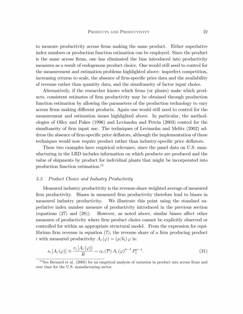
Measured industry productivity is the revenue-share weighted average of measuredfirm productivity. Biases in measured firm productivity therefore lead to biases inmeasured industry productivity. We illustrate this point using the standard su-perlative index number measure of productivity introduced in the previous section(equations (27) and (28)). However, as noted above, similar biases affect othermeasures of productivity where firm product choice cannot be explicitly observed orcontrolled for within an appropriate structural model. From the expression for equi-librium firm revenue in equation (7), the revenue share of a firm producing producti with measured productivity Ai (ϕ) = (ρ/bi)ϕ is:
si [Ai (ϕ)] ≡ri [Ai (ϕ)]
R= αi (P)Ai (ϕ)
σ−1 P σ−11 . (31)
12See Bernard et al. (2005) for an empirical analysis of variation in product mix across firms andover time for the U.S. manufacturing sector.
Products and Productivity 23
Therefore, measured industry productivity may be expressed as:
A =
Z ϕ∗∗
ϕ∗
s1 [A1 (ϕ)]A1 (ϕ) g (ϕ) dϕ
G (ϕ∗∗)−G (ϕ∗)+
Z ∞
ϕ∗∗
s2 [A2 (ϕ)]A2 (ϕ) g (ϕ) dϕ
1−G (ϕ∗∗). (32)
Proposition 4 Measured industry productivity depends on the weight of productsin consumer utility and changes in these weights will result in measured industryproductivity growth or decline.
Proof. See Appendix.
The weight of products in consumer utility, a, influences measured industry pro-ductivity through a number of routes. First, these weights determine the zero profitand product indifference cutoff productivities, ϕ∗ and ϕ∗∗, and hence the range ofproductivities where each product is produced. The product with a lower variablecost of production will have a higher measured productivity in equation (27). There-fore, other things equal, the greater the range of productivities over which the lowervariable cost product is produced, the higher measured industry productivity. Sec-ond, the weight of each product in consumer utility will affect the share of revenuereceived by a firm making each product. Other things equal, the larger the shareof revenue allocated to the product with the lower variable cost of production, thehigher measured industry productivity.Since an increase in the weight of the low variable cost product in consumer util-
ity increases both the range of productivities where the product is produced and theshare of revenue received by producers of the product, it follows that a rise in thisweight generates measured industry productivity growth. Conversely, a fall in thelow variable cost product’s weight in consumer utility generates a decline in measuredindustry productivity. Even though true firm-level productivity remains unchanged,the endogenous re-sorting of firms across products with different production tech-niques results in changes in measured industry productivity.Because firms choose products at a more disaggregated level than observed by
the empirical researcher and these products differ systematically in terms of theirtechnology, the demand-side becomes important in determining measured industryproductivity. Measured industry productivity depends on two sets of supply-sideconsiderations, the true distribution of productivity across firms and the parametersof the production technology of the two products, as well as patterns of consumerdemand which influence heterogeneous firms’ non-random decision of which productsto produce.
Products and Productivity 24
6. Deregulation and Industry Dynamics
The response of industries to policy reforms such as deregulation has been a ma-jor focus of much recent research. In this section, we use the theoretical model ofindustry equilibrium to show that endogenous product choice provides an importantadditional decision margin along which heterogeneous firms adjust to industry dereg-ulation, alongside firm entry and exit and changes in the composition of output acrossfirms of different productivities within existing product markets. We show how theendogenous sorting of firms across products may result in either measured produc-tivity growth or decline at the firm and industry level. We illustrate these responsesin the simplest possible setting by assuming a Pareto productivity distribution sothat relative prices and the relative value of the productivity cutoffs are determinedaccording to equations (25) and (26).
Proposition 5 A reduction in entry barriers, fe, leads to:(a) A rise in the zero profit productivity cutoff, ϕ∗, and a rise in the product indif-ference productivity cutoff, ϕ∗∗
(b) A rise in true average industry productivity due to exit by low productivity firms(c) Changes in measured firm productivity at surviving firms that switch products(d) Changes in measured industry productivity due to exit by low productivity firmsand switches in products at surviving firms
Proof. See Appendix.
We begin by tracing the comparative statics for the endogenous variables of themodel and for true industry productivity, before examining the implications for mea-sured firm and industry productivity. As summarized in Table 3 and proved in theAppendix, a reduction in barriers to entry (a reduction in the sunk entry cost fe) in-creases both productivity cutoff levels, thus raising true average productivity in eachproduct market and for the industry as a whole. The ratio of the productivity cut-offs, the relative price of the products, the mass of firms producing each product, andaverage profitability are unchanged. The expected value of entry falls and welfareunambiguously rises.Intuition for these results can be obtained by considering the impact of the reduc-
tion in barriers to entry at the initial steady-state equilibrium. As the sunk entrycost falls below the expected value of entry, a larger mass of firms, Me, will enter theindustry. For given values of ϕ∗ and ϕ∗∗, a larger mass of entrants implies a larger
Products and Productivity 25
mass of firms with productivity realizations high enough to produce in each market.This rise in the mass of firms producing in each market reduces ex post profitability.The reduction in ex post profitability means that some low productivity firms
are now no longer able to cover the fixed costs of producing product 1. Hence, inequilibrium the zero-profit productivity cutoff ϕ∗ rises. As ϕ∗ rises for a given valueof ϕ∗∗, this reduces the mass of firms in product 1 relative to the mass of firms inproduct 2, thereby increasing product 1’s relative profitability. Hence, some higherproductivity firms that previously made product 2 now find it more profitable toproduce the low fixed cost product 1 and ϕ∗∗ also rises.The equilibrium ratio of the two productivity cutoffs, ϕ∗∗/ϕ∗, is independent of
the sunk costs of entry, and hence ϕ∗∗ rises by the same proportion as ϕ∗. With aPareto productivity distribution, this leaves the relative price of the two products, P,unchanged.The implications of the change in barriers to entry for the two productivity cutoffs
are summarized graphically in Figure 3. The rise in both ϕ∗ and ϕ∗∗ means thatsome low productivity firms that previously made product 1 exit, while some higherproductivity firms that previously made product 2 switch to product 1. For boththese reasons, weighted average productivity in product 1, eϕ1, will rise. Since thefirms that switch from product 2 to product 1 are of lower productivity than thosewho continue to make product 2, weighted average productivity in product 2, eϕ2, willalso rise.The rise in ϕ∗ and ϕ∗∗ reduces the mass of firms with productivity realizations high
enough to produce in each market for a given mass of firms, Me, that enter. Witha Pareto distribution, this effect exactly offsets the larger mass of firms enteringthe industry, so that the mass of firms producing in each product market (M1,M2),average firm revenue (r1, r2), and average ex post profitability (π1,π2) are unchangedat the new steady-state equilibrium.The expected value of entry, ve, falls to equal the new lower sunk costs of entry, fe,
because the rise in ϕ∗ and ϕ∗∗ reduces the probability of a firm having a productivityrealization high enough to be able to profitably manufacture either product 1 orproduct 2. Welfare per worker, W , rises because, although the mass of firms andhence product varieties is unchanged, the rise in average productivity within eachproduct market reduces average variety prices and hence consumer price indices.The implications of the fall in entry barriers for true productivity can be sum-
marized as follows. True productivity at the firm-level remains unchanged becauseit is drawn from a distribution at the point of entry. True average industry pro-
Products and Productivity 26
ductivity rises due to exit by low productivity firms. Besides these implications fortrue productivity, endogenous changes in product by surviving firms have additionalconsequences for measured productivity at both the firm and industry level.Consider the standard superlative index number measures of productivity intro-
duced in equation (28) for the firm and equation (32) for the industry. Higherproductivity surviving firms that switch from product 2 to product 1 may experienceeither measured productivity growth or decline depending on whether the variablecost of production for product 1 is lower or higher than the variable cost of productionfor product 2 respectively. For all other surviving firms, measured firm productivitywill remain unchanged.Measured industry productivity will be influenced both by exit by low productivity
firms and by endogenous changes in product at surviving firms. With an unchangedrelative price for the two products, P, the share of revenue received by a firm makinga given product in equation (32) will remain unchanged. If product 1 has a lowervariable cost of production than product 2, switches in products will reinforce theincrease in measured average industry productivity due to exit by low productivityfirms. If product 1 has a higher variable cost of production than product 2, theendogenous changes in products will reduce measured average industry productivity,and if this reduction is large enough to offset the effect of exit by low productivityfirms, measured industry productivity may decline.We have illustrated the point that endogenous choice between heterogeneous prod-
ucts provides a new margin of adjustment to deregulation that influences measuredfirm and industry productivity using standard superlative index number measures ofproductivity assuming perfect competition and constant returns to scale. However,as we showed above, similar biases will affect any other productivity measure whereinformation on price, cost, output and input is not available at the firm-product levelor where endogenous product choice cannot be modelled using a structural model ofindustry equilibrium.These points are not specific to the particular theoretical framework considered
here. Similar measurement problems will be present whenever firm product choiceis made at a more finely detailed level than observed by empirical researchers andwhere products differ in terms of production technique or the way in which theyenter demand. Explicitly modelling the endogenous sorting of firms across productswithin industries will help to deepen our understanding of how industries respond toderegulation and the heterogeneous responses of measured productivity across firmsand industries to exogenous policy reform.
Products and Productivity 27
7. Conclusions
Firms’ decisions about what products to produce are often made at a more dis-aggregate level than observed by empirical researchers. When products differ inproduction techniques or the way in which they enter demand, this aggregation prob-lem introduces a bias into standard productivity measures. In general, when productsvary in production technique, the standard identifying assumption that technologiesare the same across firms within industries up to a Hicks-neutral or factor augment-ing productivity shifter will be violated. As a result, productivity measures will bebiased even if firm-specific data is available on prices and costs and on the physicalquantity of output rather than revenue.The paper develops a theoretical model of industry equilibrium where endoge-
nous self-selection into products may magnify measured productivity dispersion acrossfirms within industries, and where changes in the relative demand for products maygenerate measured industry productivity growth. Measured productivity reflects notonly the true underlying characteristics of firms but also their non-random decision ofwhat product to produce. The endogenous sorting of firms across products influencesthe response of industries to exogenous policy reforms such as industry deregulation.Reductions in barriers to entry raise true industry productivity due to increased exitby low productivity firms, but measured firm and industry productivity may eitherrise or decline due to endogenous switches by surviving firms between products withheterogeneous characteristics.Our analysis suggests a number of areas for further empirical inquiry. Researchers
should make use of existing data on the evolving product mix of firms. In someinstances these data may only be available for particular markets and industries,but even comprehensive data sources such as the U.S. Census Bureau’s Longitudi-nal Research Database contain much information on firms’ product-level production.Bernard et al. (2005), for example, find that U.S. firms within industries vary sub-stantially in terms of their product mix.Further theoretical research is also warranted, particularly in developing richer
models of industry dynamics that allow firms to choose the number and type ofgoods they produce. While product choice introduces an additional dimension offirm heterogeneity to track over time, it promises to yield new insights into how firms,industries and economies respond to exogenous changes in the economic environmentand policy regime.
Products and Productivity 28
References
Baily, N, Hulten, C and Campbell, D (1992) "Productivity Dynamics in Manufactur-ing Plants", Brookings Papers on Economic Activity, Microeconomics, 187-267.
Bernard, Andrew B., Stephen Redding, and Peter K. Schott, (2005) "Multi-ProductFirms, Industry Mix, and Product Switching", Tuck School of Business at Dart-mouth, mimeo.
Berry, S, Levinsohn, J and Pakes, A (1995) "Automobile Prices in Market Equilib-rium", Econometrica, 63, 841-90.
Caves D., Christensen L., and Diewert E., (1982a) "The Economic Theory of IndexNumbers and the Measurement of Input, Output and Productivity", Economet-rica, 50(6): 1393-1414.
Caves D., Christensen L., and Diewert E., (1982b) "Multilateral Comparisons ofOutput, Input and Productivity Using Superlative Index Numbers", EconomicJournal, 92, 73-86.
Davis, Steven J and John Haltiwanger. (1991) "Wage Dispersion between and withinU.S. Manufacturing Plants, 1963-86." Brookings Papers on Economic Activity,Microeconomics, pp. 115-80.
De Loecker, J (2005) "Product Differentiation, Multi-Product Firms and StructuralEstimation of Productivity", K.U. Leuven, mimeograph.
Disney, R, Haskel, J and Heden, Y (2003) "Restructuring and Productivity Growthin UK Manufacturing", Economic Journal, 113, 666-94.
Dunne, T., Roberts M. J., and Samuelson L., (1989) "The Growth and Failure ofU.S. Manufacturing Plants", Quarterly Journal of Economics, 104(4):671-98..
Ericsson, Richard and Pakes, Ariel (1995) "Markov-Perfect Industry Dynamics: AFramework for Empirical Work", Review of Economic Studies, 62(1), 53-82.
Foster, L, Haltiwanger, J and Krizan, C (2002) "The Link Between Aggregate andMicro Productivity Growth: Evidence from Retail Trade", NBERWorking Paper,#9120.
Products and Productivity 29
Foster, L, Haltiwanger, J and Krizan, C (2001) “Aggregate Productivity Growth:Lessons from Microeconomic Evidence.” in New Developments in ProductivityAnalysis, Hulten, Charles R; Dean, Edwin R; Harper, Michael J, eds, NBERStudies in Income andWealth, vol. 63. Chicago and London: University of ChicagoPress.
Goldberg, Pinelopi Koujianou (1995) “Product Differentiation and Oligopoly in In-ternational Markets: The Case of the U.S. Automobile Industry.” Econometrica891-951.
Hall, R (1988) "The Relationship Between Price and Marginal Cost in US Industry",Journal of Political Economy, 96(5):921-947
Hausman, J (1997) "Valuation of New Goods under Perfect and Imperfect Compe-tition", in (eds) Bresnahan, T and Gordon, R, The Economics of New Goods,Chicago University Press and NBER.
Hopenhayn, Hugo. (1992) "Entry, Exit, and Firm Dynamics in Long Run Equilib-rium." Econometrica, 60(5): 1127-1150.
Hotelling, H. (1929) "Stability in Competition." Economic Journal, 39: 41-57.
Jovanovic, Boyan. (1982) "Selection and the Evolution of Industry." Econometrica,vol. 50(3): 649-70.
Katayama, H, Lu, S and Tybout, J (2003) "Why Plant-Level Productivity Studies areOften Misleading, and an Alternative Approach to Interference", NBER WorkingPaper, 9617.
Klette, T and Griliches, Z (1996) "The Inconsistency of Common Scale Estimatorswhen Output Prices are Unobserved and Endogenous", Journal of Applied Econo-metrics, 11:343-61.
Lancaster, Kelvin. (1966), "A New Approach to Consumer Theory." Journal of Po-litical Economy, 74: 132-157.
Levinsohn, J and Melitz, M (2002) "Productivity in a Differentiated Products MarketEquilibrium", Harvard University, mimeograph.
Levinsohn, J and Petrin, A (2003) "Estimating Production Functions Using Inputsto Control for Unobservables", Review of Economic Studies, 70:317-41.

Products and Productivity 30
Martin, R (2005) "Computing the True Spread", Centre for Economic PerformanceDiscussion Paper, 0692.
Melitz, Marc J. (2003). The Impact of Trade on Intra-Industry Reallocations andAggregate Industry Productivity. Econometrica 71: 1695-1725.
Olley, Steven G. and Ariel Pakes, (1996) "The Dynamics of Productivity in theTelecommunications Equipment Industry." Econometrica, 64(6): 1263-97.
Pavcnik, N (2002) ‘Trade Liberalization, Exit, and Productivity Improvement: Evi-dence from Chilean Plants’, Review of Economic Studies, 69(1): 245-76.
Petrin, A (2002) "Quantifying the Benefits of New Products: The Case of the Mini-van", Journal of Political Economy, 110(4): 705-29.
Roeger, W. (1995) "Can Imperfect Competition Explain the Difference Between Pri-mal and Dual Productivity Measures? Estimates for US Manufacturing", Journalof Political Economy, 103(2): 316-30.
Shaked, Avner and Sutton, John. (1982) "Imperfect Information, Perceived Quality,and the Formation of Professional Groups." Journal of Economic Theory 27(1):170-81.
Spence, A. Michael. (1976) "Product Differentiation and Welfare." American Eco-nomic Review, 66(2):407-414.
Sutton, John. (1998) Technology and Market Structure: Theory and History, MITPress, Cambridge, Massachusetts.
Syverson, Chad (2004) "Market Structure and Productivity: A Concrete Example",Journal of Political Economy, 112(6): 1181-222.
Trajtenberg, M (1989) "The Welfare Analysis of Product Innovations, with an Ap-plication to Computed Tomography Scanners", Journal of Political Economy, 97:444-79.
Tybout, J, de Melo, J, and Corbo, V (1991) "The Effects of Trade Reforms on Scaleand Technical Efficiency: New Evidence from Chile", Journal of InternationalEconomics, 31(3-4): 231-50.

Products and Productivity 31
U.S. Census Bureau. (1996) "1992 Census of Manufactures: Numerical List of Man-ufactured and Mineral Products." U.S. Government Printing Office, WashingtonDC. http://www.census.gov/prod/2/manmin/mc92-r-1.pdf
Products and Productivity 32
A Appendix: Theoretical Derivations
A1. Weighted Average Productivity and Average Profitability
eϕ1 (ϕ∗, ϕ∗∗) =
∙1
G (ϕ∗∗)−G (ϕ∗)
Z ϕ∗∗
ϕ∗ϕσ−1g (ϕ) dϕ
¸1/(σ−1)(33)
eϕ2 (ϕ∗∗) =
∙1
1−G (ϕ∗∗)
Z ∞
ϕ∗∗ϕσ−1g (ϕ) dϕ
¸1/(σ−1)Using the relationship between the revenues of firms producing varieties in the
same and in different markets, as well as the expression for the zero-profit productivitycutoff and the CES expenditure share, average profit in the two product markets,πi = πi (ϕi) may be written as follows:
π1(ϕ∗, ϕ∗∗) =
"µeϕ1 (·)ϕ∗
¶σ−1− 1#f1 (34)
π2(ϕ∗, ϕ∗∗,P) =
"µ1− a
a
¶ψ µ1
b
eϕ2 (·)ϕ∗
¶σ−1Pσ−ψ − f2
f1
#f1 (35)
A2. Proof of Proposition 1
Proof. We begin by determining the equilibrium sextuple: ϕ∗, ϕ∗∗, P1, P2, R1, R2.First, we use the relative supply and relative demand relationships in equations (21)and (22) to establish that there exist unique equilibrium values of ϕ∗∗/ϕ∗ and P.Rearranging the product supply relationship, we obtain:
P = bσ−1σ−ψ
µa
1− a
¶ ψσ−ψ
"µϕ∗∗
ϕ∗
¶1−σ µf2f1− 1¶+ 1
# 1σ−ψ
. (36)
Since σ > 1, the right-hand side is monotonically decreasing in ϕ∗∗/ϕ∗ and is graphedin (P, ϕ∗∗/ϕ∗) space in Figure 2. P takes the value (f2/f1)1/(σ−ψ) (a/(1− a))ψ/(σ−ψ) b(σ−1)/(σ−ψ) >
0 at ϕ∗∗/ϕ∗ = 1 and converges to a lower value of (a/(1− a))ψ/(σ−ψ) b(σ−1)/(σ−ψ) > 0
as ϕ∗∗/ϕ∗ tends to infinity.Turning now to the product demand relationship (equation (22)), the left-hand sideis monotonically increasing in ϕ∗∗/ϕ∗ and is also graphed in (P, ϕ∗∗/ϕ∗) space below.As ϕ∗∗/ϕ∗ approaches 1, P converges to 0. As ϕ∗∗/ϕ∗ tends to infinity, P convergesto ∞.
Products and Productivity 33
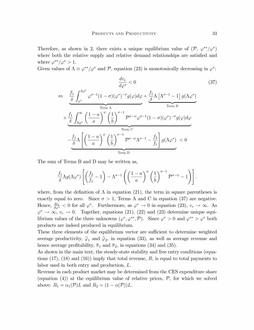
Therefore, as shown in 2, there exists a unique equilibrium value of (P, ϕ∗∗/ϕ∗)where both the relative supply and relative demand relationships are satisfied andwhere ϕ∗∗/ϕ∗ > 1.Given values of Λ ≡ ϕ∗∗/ϕ∗ and P, equation (23) is monotonically decreasing in ϕ∗:
dvedϕ∗
< 0 (37)
⇔ f1δ
Z Λϕ∗
ϕ∗ϕσ−1(1− σ)(ϕ∗)−σg(ϕ)dϕ| z
Term A
+f1δΛ£Λσ−1 − 1
¤g(Λϕ∗)| z
Term B
+f1δ
Z ∞
Λϕ∗
µ1− a
a
¶ψ µ1
b
¶σ−1Pσ−ψϕσ−1(1− σ)(ϕ∗)−σg(ϕ)dϕ| z
Term C
−f1δΛ
"µ1− a
a
¶ψ µ1
b
¶σ−1Pσ−ψΛσ−1 − f2
f1
#g(Λϕ∗)| z
Term D
< 0
The sum of Terms B and D may be written as,
f1δΛg(Λϕ∗)
"µf2f1− 1¶− Λσ−1
õ1− a
a
¶ψ µ1
b
¶σ−1Pσ−ψ − 1
!#.
where, from the definition of Λ in equation (21), the term in square parentheses isexactly equal to zero. Since σ > 1, Terms A and C in equation (37) are negative.Hence, dve
dϕ∗ < 0 for all ϕ∗. Furthermore, as ϕ∗ → 0 in equation (23), ve → ∞. Asϕ∗ → ∞, ve → 0. Together, equations (21), (22) and (23) determine unique equi-librium values of the three unknowns (ϕ∗, ϕ∗∗,P). Since ϕ∗ > 0 and ϕ∗∗ > ϕ∗ bothproducts are indeed produced in equilibrium.These three elements of the equilibrium vector are sufficient to determine weightedaverage productivity, eϕ1 and eϕ2, in equation (33), as well as average revenue andhence average profitability, π1 and π2, in equations (34) and (35).As shown in the main text, the steady-state stability and free entry conditions (equa-tions (17), (18) and (16)) imply that total revenue, R, is equal to total payments tolabor used in both entry and production, L.Revenue in each product market may be determined from the CES expenditure share(equation (4)) at the equilibrium value of relative prices, P, for which we solvedabove: R1 = α1(P)L and R2 = (1− α(P))L.
Products and Productivity 34
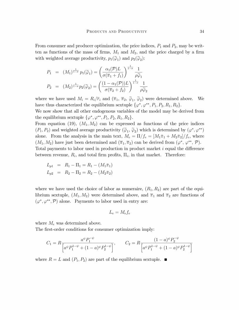
From consumer and producer optimization, the price indices, P1 and P2, may be writ-ten as functions of the mass of firms, M1 and M2, and the price charged by a firmwith weighted average productivity, p1(eϕ1) and p2(eϕ2):
P1 = (M1)1
1−σ p1(eϕ1) = µ α1(P)Lσ(π1 + f1)
¶ 11−σ 1
ρeϕ1P2 = (M2)
11−σ p2(eϕ2) = µ(1− α1(P))L
σ(π2 + f2)
¶ 11−σ 1
ρeϕ2where we have used Mi = Ri/ri and (π1, π2, eϕ1, eϕ2) were determined above. Wehave thus characterized the equilibrium sextuple ϕ∗, ϕ∗∗, P1, P2, R1, R2.We now show that all other endogenous variables of the model may be derived fromthe equilibrium sextuple ϕ∗, ϕ∗∗, P1, P2, R1, R2.From equation (19), (M1,M2) can be expressed as functions of the price indices(P1, P2) and weighted average productivity (eϕ1, eϕ2) which is determined by (ϕ∗, ϕ∗∗)alone. From the analysis in the main text, Me = Π/fe = [M1π1 +M2π2]/fe, where(M1,M2) have just been determined and (π1, π2) can be derived from (ϕ∗, ϕ∗∗, P).Total payments to labor used in production in product market i equal the differencebetween revenue, Ri, and total firm profits, Πi, in that market. Therefore:
Lp1 = R1 −Π1 = R1 − (M1π1)
Lp2 = R2 −Π2 = R2 − (M2π2)
where we have used the choice of labor as numeraire, (R1, R2) are part of the equi-librium sextuple, (M1,M2) were determined above, and π1 and π2 are functions of(ϕ∗, ϕ∗∗,P) alone. Payments to labor used in entry are:
Le =Mefe
where Me was determined above.The first-order conditions for consumer optimization imply:
C1 = RaψP−ψ1h
aψP 1−ψ1 + (1− a)ψP 1−ψ
2
i , C2 = R(1− a)ψP−ψ2h
aψP 1−ψ1 + (1− a)ψP 1−ψ2
iwhere R = L and (P1, P2) are part of the equilibrium sextuple.
Products and Productivity 35
B Proof of Proposition 2
Proof. This Proposition follows immediately from the Proof of Proposition 1 wherewe have established that ϕ∗ > 0 and ϕ∗∗ > ϕ∗.
C Proof of Proposition 3
Proof. The Proposition follows immediately from equation (28). Compare a firmwith productivity ϕ0 > ϕ00 making product 2 to a firm with productivity ϕ00 makingproduct 1. Relative measured productivity of the two firms is equal to:
A (ϕ0)
A (ϕ00)=
ϕ0
ϕ001
b(38)
D Proof of Corollary 1
Proof. The Proposition follows immediately from Propositions 2 and 3. Sincef2 > f1, product 2 is produced by higher productivity firms. Compare a firm withproductivity ϕ0 > ϕ00 making product 2 to a firm with productivity ϕ00 making product1. If b2 < b1, then 0 < b < 1, and from equation (38):
A (ϕ0)
A (ϕ00)>
ϕ0
ϕ00(39)
E Proof of Proposition 4
Proof. From equation (31) and (4), an increase in the weight of a product in consumerutility a, (1− a) raises the share of revenue allocated to a producer of that productand reduces the share of revenue allocated to a producer of the other product. Ifproducts differ in terms of their variable cost of production, A2 (ϕ) 6= A1 (ϕ), anincrease in the weight of a product in consumer utility will influence measured industryproductivity through the numerators in equation (32).From equations (21), (22) and (23), an increase in the weight of a product in consumerutility a, (1− a) will also affect the zero profit and product indifference productivitycutoffs ϕ∗, ϕ∗∗ and hence the range of productivities over which the two productsare produced. The share of revenue received, si [Ai (ϕ)], and measured productivity,
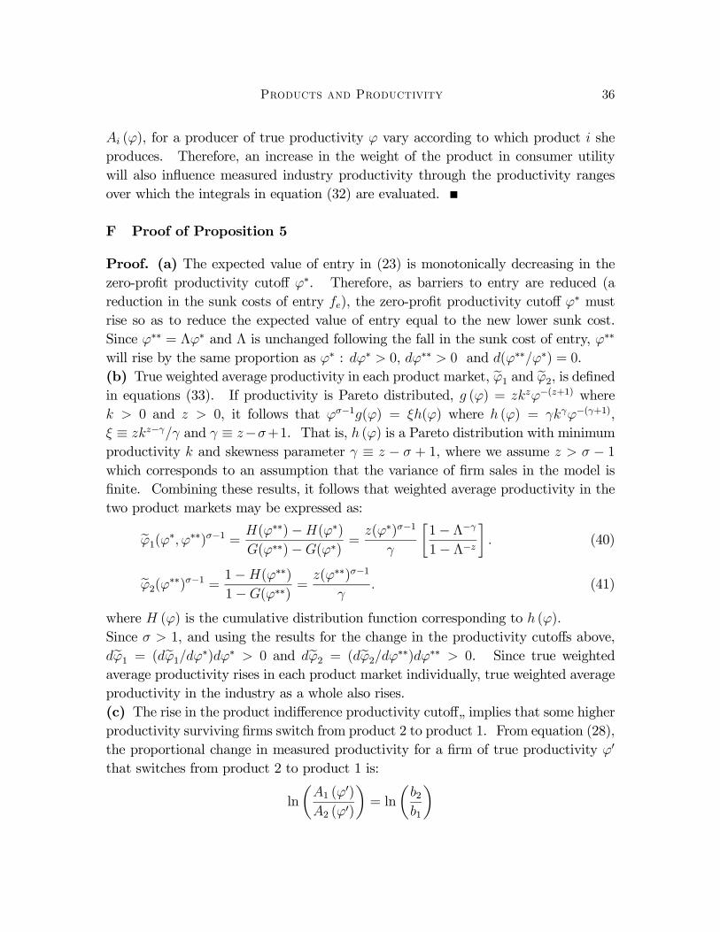
Products and Productivity 36
Ai (ϕ), for a producer of true productivity ϕ vary according to which product i sheproduces. Therefore, an increase in the weight of the product in consumer utilitywill also influence measured industry productivity through the productivity rangesover which the integrals in equation (32) are evaluated.
F Proof of Proposition 5
Proof. (a) The expected value of entry in (23) is monotonically decreasing in thezero-profit productivity cutoff ϕ∗. Therefore, as barriers to entry are reduced (areduction in the sunk costs of entry fe), the zero-profit productivity cutoff ϕ∗ mustrise so as to reduce the expected value of entry equal to the new lower sunk cost.Since ϕ∗∗ = Λϕ∗ and Λ is unchanged following the fall in the sunk cost of entry, ϕ∗∗
will rise by the same proportion as ϕ∗ : dϕ∗ > 0, dϕ∗∗ > 0 and d(ϕ∗∗/ϕ∗) = 0.(b) True weighted average productivity in each product market, eϕ1 and eϕ2, is definedin equations (33). If productivity is Pareto distributed, g (ϕ) = zkzϕ−(z+1) wherek > 0 and z > 0, it follows that ϕσ−1g(ϕ) = ξh(ϕ) where h (ϕ) = γkγϕ−(γ+1),ξ ≡ zkz−γ/γ and γ ≡ z−σ+1. That is, h (ϕ) is a Pareto distribution with minimumproductivity k and skewness parameter γ ≡ z − σ + 1, where we assume z > σ − 1which corresponds to an assumption that the variance of firm sales in the model isfinite. Combining these results, it follows that weighted average productivity in thetwo product markets may be expressed as:
eϕ1(ϕ∗, ϕ∗∗)σ−1 = H(ϕ∗∗)−H(ϕ∗)
G(ϕ∗∗)−G(ϕ∗)=
z(ϕ∗)σ−1
γ
∙1− Λ−γ
1− Λ−z
¸. (40)
eϕ2(ϕ∗∗)σ−1 = 1−H(ϕ∗∗)
1−G(ϕ∗∗)=
z(ϕ∗∗)σ−1
γ. (41)
where H (ϕ) is the cumulative distribution function corresponding to h (ϕ).Since σ > 1, and using the results for the change in the productivity cutoffs above,deϕ1 = (deϕ1/dϕ∗)dϕ∗ > 0 and deϕ2 = (deϕ2/dϕ∗∗)dϕ∗∗ > 0. Since true weightedaverage productivity rises in each product market individually, true weighted averageproductivity in the industry as a whole also rises.(c) The rise in the product indifference productivity cutoff„ implies that some higherproductivity surviving firms switch from product 2 to product 1. From equation (28),the proportional change in measured productivity for a firm of true productivity ϕ0
that switches from product 2 to product 1 is:
ln
µA1 (ϕ
0)
A2 (ϕ0)
¶= ln
µb2b1
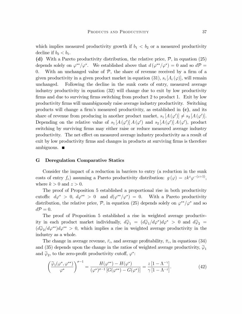
Products and Productivity 37
which implies measured productivity growth if b1 < b2 or a measured productivitydecline if b2 < b1.(d) With a Pareto productivity distribution, the relative price, P, in equation (25)depends solely on ϕ∗∗/ϕ∗. We established above that d (ϕ∗∗/ϕ∗) = 0 and so dP =0. With an unchanged value of P, the share of revenue received by a firm of agiven productivity in a given product market in equation (31), si [Ai (ϕ)], will remainunchanged. Following the decline in the sunk costs of entry, measured averageindustry productivity in equation (32) will change due to exit by low productivityfirms and due to surviving firms switching from product 2 to product 1. Exit by lowproductivity firms will unambiguously raise average industry productivity. Switchingproducts will change a firm’s measured productivity, as established in (c), and itsshare of revenue from producing in another product market, s1 [A (ϕ0)] 6= s2 [A (ϕ
0)].Depending on the relative value of s1 [A (ϕ0)]A (ϕ0) and s2 [A (ϕ
0)]A (ϕ0), productswitching by surviving firms may either raise or reduce measured average industryproductivity. The net effect on measured average industry productivity as a result ofexit by low productivity firms and changes in products at surviving firms is thereforeambiguous.
G Deregulation Comparative Statics
Consider the impact of a reduction in barriers to entry (a reduction in the sunkcosts of entry fe) assuming a Pareto productivity distribution: g (ϕ) = zkzϕ−(z+1),where k > 0 and z > 0.The proof of Proposition 5 established a proportional rise in both productivity
cutoffs: dϕ∗ > 0, dϕ∗∗ > 0 and d(ϕ∗∗/ϕ∗) = 0. With a Pareto productivitydistribution, the relative price, P, in equation (25) depends solely on ϕ∗∗/ϕ∗ and sodP = 0.The proof of Proposition 5 established a rise in weighted average productiv-
ity in each product market individually, deϕ1 = (deϕ1/dϕ∗)dϕ∗ > 0 and deϕ2 =(deϕ2/dϕ∗∗)dϕ∗∗ > 0, which implies a rise in weighted average productivity in theindustry as a whole.The change in average revenue, ri, and average profitability, πi, in equations (34)
and (35) depends upon the change in the ratios of weighted average productivity, eϕ1and eϕ2, to the zero-profit productivity cutoff, ϕ∗:µeϕ1(ϕ∗, ϕ∗∗)
ϕ∗
¶σ−1=
H(ϕ∗∗)−H(ϕ∗)
(ϕ∗)σ−1 [G(ϕ∗∗)−G(ϕ∗)]=
z [1− Λ−γ]
γ [1− Λ−z]. (42)
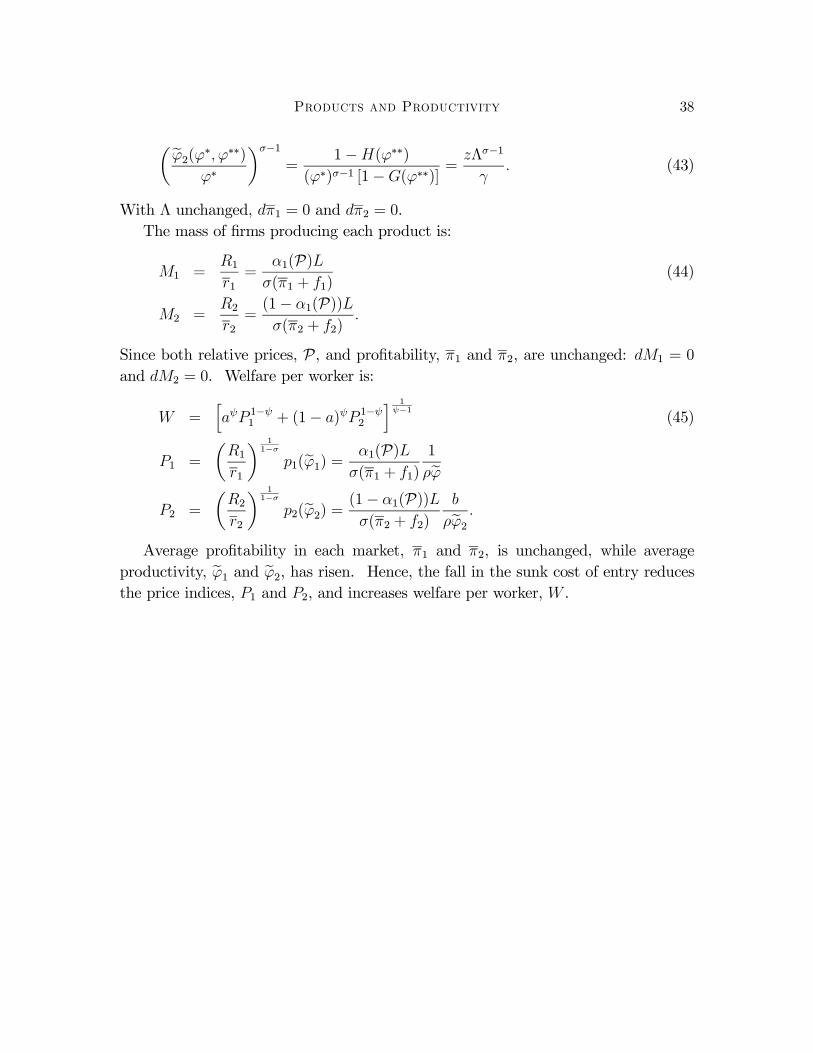
Products and Productivity 38
µeϕ2(ϕ∗, ϕ∗∗)ϕ∗
¶σ−1=
1−H(ϕ∗∗)
(ϕ∗)σ−1 [1−G(ϕ∗∗)]=
zΛσ−1
γ. (43)
With Λ unchanged, dπ1 = 0 and dπ2 = 0.The mass of firms producing each product is:
M1 =R1r1=
α1(P)Lσ(π1 + f1)
(44)
M2 =R2r2=(1− α1(P))Lσ(π2 + f2)
.
Since both relative prices, P, and profitability, π1 and π2, are unchanged: dM1 = 0
and dM2 = 0. Welfare per worker is:
W =haψP 1−ψ
1 + (1− a)ψP 1−ψ2
i 1ψ−1
(45)
P1 =
µR1r1
¶ 11−σ
p1(eϕ1) = α1(P)Lσ(π1 + f1)
1
ρeϕP2 =
µR2r2
¶ 11−σ
p2(eϕ2) = (1− α1(P))Lσ(π2 + f2)
b
ρeϕ2 .Average profitability in each market, π1 and π2, is unchanged, while average
productivity, eϕ1 and eϕ2, has risen. Hence, the fall in the sunk cost of entry reducesthe price indices, P1 and P2, and increases welfare per worker, W .
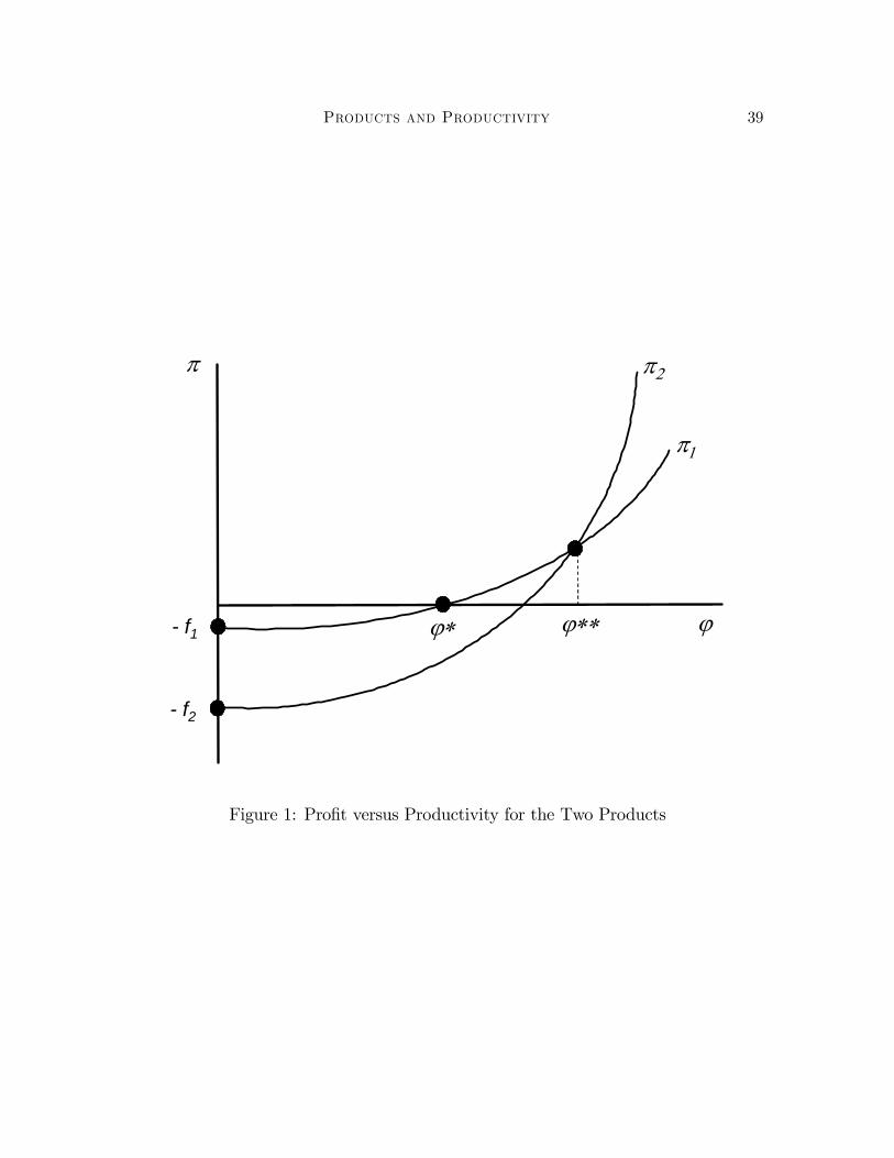
Products and Productivity 39
- f2
- f1
π π2
π1
ϕϕ∗ ϕ∗∗
Figure 1: Profit versus Productivity for the Two Products
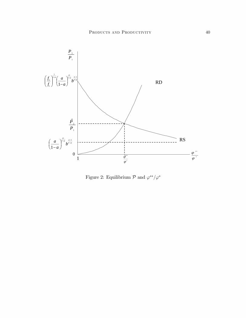
Products and Productivity 40
01
1
2
PP
*
**
ϕϕ
RD
RS
1
2ˆPP
*
**ˆϕϕ
ψσσψσ
ψψσ
−−−−
⎟⎠⎞
⎜⎝⎛−⎟⎟
⎠
⎞⎜⎜⎝
⎛ 11
1
2
1b
aa
ff
ψσσψσ
ψ
−−−
⎟⎠⎞
⎜⎝⎛−
1
1b
aa
Figure 2: Equilibrium P and ϕ∗∗/ϕ∗
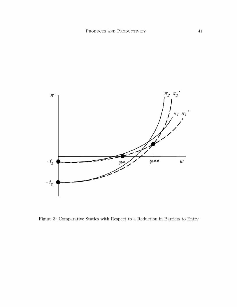
Products and Productivity 41
- f2
- f1
π π2
π1
ϕϕ∗ ϕ∗∗
π2’
π1’
Figure 3: Comparative Statics with Respect to a Reduction in Barriers to Entry
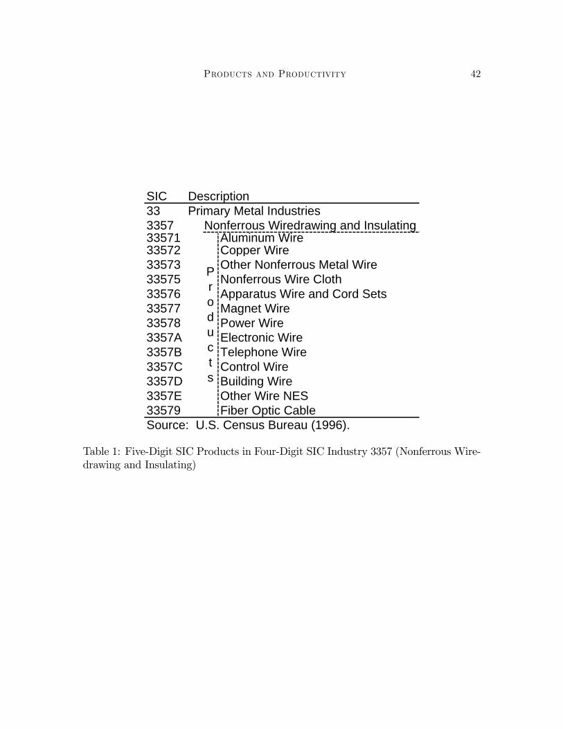
Products and Productivity 42
SIC Description33 Primary Metal Industries3357 Nonferrous Wiredrawing and Insulating33571 Aluminum Wire33572 Copper Wire33573 Other Nonferrous Metal Wire33575 Nonferrous Wire Cloth33576 Apparatus Wire and Cord Sets33577 Magnet Wire33578 Power Wire3357A Electronic Wire3357B Telephone Wire3357C Control Wire3357D Building Wire3357E Other Wire NES33579 Fiber Optic CableSource: U.S. Census Bureau (1996).
Products
Table 1: Five-Digit SIC Products in Four-Digit SIC Industry 3357 (Nonferrous Wire-drawing and Insulating)
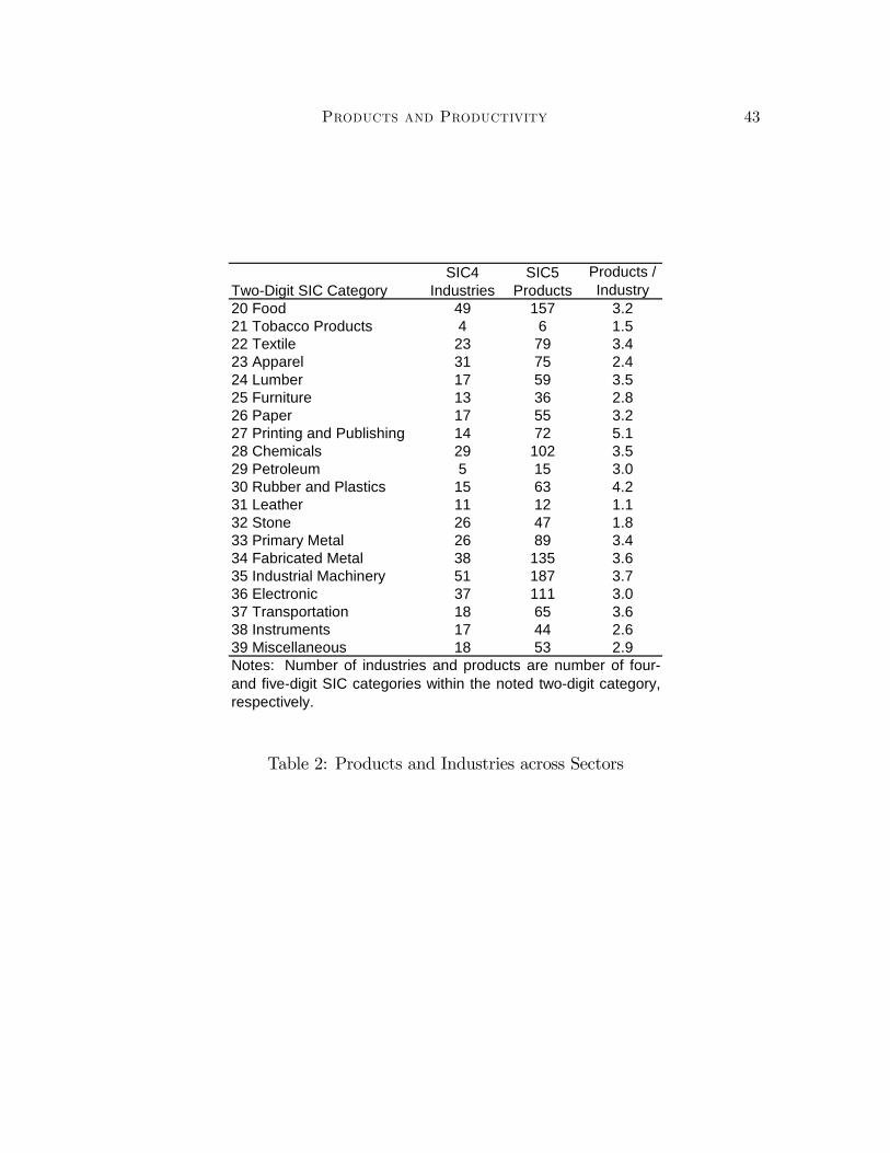
Products and Productivity 43
SIC4 SIC5Two-Digit SIC Category Industries Products20 Food 49 157 3.221 Tobacco Products 4 6 1.522 Textile 23 79 3.423 Apparel 31 75 2.424 Lumber 17 59 3.525 Furniture 13 36 2.826 Paper 17 55 3.227 Printing and Publishing 14 72 5.128 Chemicals 29 102 3.529 Petroleum 5 15 3.030 Rubber and Plastics 15 63 4.231 Leather 11 12 1.132 Stone 26 47 1.833 Primary Metal 26 89 3.434 Fabricated Metal 38 135 3.635 Industrial Machinery 51 187 3.736 Electronic 37 111 3.037 Transportation 18 65 3.638 Instruments 17 44 2.639 Miscellaneous 18 53 2.9Notes: Number of industries and products are number of four-and five-digit SIC categories within the noted two-digit category,respectively.
Products / Industry
Table 2: Products and Industries across Sectors

Products and Productivity 44
dϕ∗ > 0 dϕ∗∗ > 0
d (ϕ∗∗/ϕ∗) = 0 dP = 0deϕ1(ϕ∗, ϕ∗∗) > 0 deϕ2(ϕ∗∗) > 0dr1 = 0 dr2 = 0
dπ1 = 0 dπ2 = 0
dM1 = 0 dM2 = 0
dve < 0 dW > 0
Table 3: Comparative Statics with Respect to a Reduction in Barriers to Entry (afall in sunk entry costs fe) .