NCLASSIFIED .3 E/////// COLLEGE DEPT OF OCEANOGRAPHY ... · PDF fileADA03 536 TEXAS A AND UNIV COLLEGE STATION DEPT OF OCEANOGRAPHY F/6 ... Doctor of Philosophy ... committee, Dr

ADA03 536 TEXAS A AND UNIV COLLEGE STATION DEPT OF OCEANOGRAPHY F/6 8/4GEOCHE ISTRY OF DISSOLVED GASES IN THE HYPERSALINE ORCA BASIN.(U)

DEC 80 D A SIESL4JR N0001-75-C-0537NCLASSIFIED TANJREF-0-1l-T.3 E///////....hhhEElhEEEEEEEEhmmhmmhhhhlhEEI-EhhEEllhIEhlEElhElhElhEhmhhhhmhhhhhuhmhmhmmhhh.

LEVELA

GEOCHEMISTRY OF DISSOLVED GASES IN THEHYPERSALINE ORCA BASIN

TECHNICAL REPORTby

Denis A. Wlesenburg

Reference 80-14-TDecember 1980 tol

I Sponsored byiJ OFFICE OF NAVAL RESEARCHLL.

Contracts N00014-75-C-0537 and N00014-80-C-00113

* 1 9 01 023

- - ,TE

MANDATORY DISTRIBUTION LIST

FOR UNCLASSIFIED TECHNICAL REPORTS, REPRINTS & FINAL REPORTSPUBLISHED BY OCEANOGRAPHIC CONTRACTORS

OF THE OCEAN SCIENCE AND TECHNOLOGY DIVISIONSOF THE OFFICE OF NAVAL RESEARCH

(REVISED NOV. 1978)

Deputy Under Secretary of Defense(Research and Advanced Technology)Military Assistant for Environmental ScienceRoom 3D129Washington, DC 20301

Office of Naval Research800 North Quincy StreetArlington, VA 22217

3 * ATTN: Code 483*1 ATTN: Code 4602 ATTN: 102B

1 ResRep (if any) -H--------- Mr. Frank Lucas or Robert PrestridgeONR Resident Representative

Commanding Officer Room 582, Federal BuildingNaval Research Laboratory 300 E. 8th StreetWashington, DC 20375 Austin, TX 78701

6 ATTN: Library, Code 2627

12*-, Defense Documentation CenterCameron StationAlexandria, VA 22314ATTN: DCA

CommanderNaval Oceanographic OfficeNSTL STationBay St. Louis, MS 39522

1 Attn: Code 81001 Attn: Code 60001 Attn: Code 3300

1 NODC/NOAACode D781Wisconsin Avenue, N.W.Washington, D.C. 20235

* Add one separate copy ofForm DD-1473

* * Send with these 12 copies two completed forms DDC-50one self addressed back to the contractor, then theother addressed to ONR, Code 480.

UNCLASSIFIED

SECURITY CLASSIFICATION Of THIS P04GE (noeen Data Entered)

REPORT DOCUMENTATION PAGE BEFOE COMPLTINGORM

lN ............ - j 2. GOVT' ACCSSION NO 3. RECIPIENT'S CATALOG NUMBER

X-. 1Ct & ,'C..tit , . TYPE OF REPORT a PEIOD COVEREDrbechnical Rep'Qtt.Jj GEOCHEMISTRY OFAISSOLVED..fASES IN e at

.---- THE HYPERSALINES.A BASIN 6 PERFORMING ORG. REPORT NUMBER.... .. ............ ....... . .. _ _8 0 -14 -T

7. AUTNOR(s) S. CONTRACT OR GRANT NUMSEI.()

DENIS A/'WIESENBURG b NO0014-8-C-I13 9

9. PERFORMING ORGANIZATION NAME AND ADDRESS 10. PROGRAM ELEMENT. PROJECT. TASKAREA S WORK UNIT NUMBERS

Department of Oceanography 3200A-9 & 4200-9Texas A&M UniversityCollege Station, Texas 77843 NR 083-036

It. CONTROLLING OFFICE NAME AND ADDRESS X12. REPORT DATE

Office of Naval Research - ecm 180Code 480Arlinqton, Va. 22217 282

14. MONITORING AGENCY NAME & AOORESS(II differet boon Conlrolling Office) IS. SECURITY CLASS. (of this report)

Texas A & M Research Foundation UNCLASSIFIEDFaculty Exchange Box HTexas A&M University 1s. DECL ASSI FICATION/ DOWNGRADING

College Station, Texas 77843 SCNEDULE

IS. DISTRIBUTION STATEMENT (of this Report)

Approved for public release, distribution unlimited., z-.v

17. OISTRIBUTION STATEMENT (of Che abetract entered In Block 20. it different bom Rept) ,

Approved for public release, distribution unlimited.

IS. SUPPLEMENTARY NOTES

IS. KEY WORDS (Contliue .on ee edo It necessary amd Idenuif7 by block mhbr)

Orca Basin Anaerobic decompositonBrine poolDissolved gases

20. A6STfACT (Centimes an revere sEd Ife neceesar and Identify by blok number)* . . ' Hypersaline, anoxic waters significantly affect the biogeochemistry

of dissolved gases in the Orca Basin (northern Gulf of Mexico). The highstability of the Orca brine pool makes it an ideal laboratory forstudying production and consumption of dissolved gases during anaerobicdecomposition. Depth distributions were determined for nitrogen, oxygen,argon, methane, ethane, propane, ammonia, hydrogen sulfide, and nitrous-,

(OVER)

D R 1473 EDITION OF NOYV 0 IS OSSOLETE CAJ " "

CIOCCUIITY CL ASIFICATION OF T4IS PAGE (Men. Oafs 0040

(I

20. ABSTRACT (cont.)

--oxide. Physical stratification of the water column stronglyinfluences Orca Basin gas distributions. The high salinitybrine (",250%/o) is internally well mixed due to convectiveoverturning, but transfer across the brine-sea water interfaceis controlled by-molecular diffusion. With a moleculardiffusivity of l0-cm . sec- , it will take 10 years for allsalts to diffuse fro'i-te-basin. Heat diffuses faster than saltand is lost from the basin at a rate of 0.5!.pial .cm2 ,-sec-1 .If geothermal heat input from the sediments is slightly higher,this input could account for the higher temperature in the brine(5.6C) compared to the deep Gulf waters (4.2PC).

This study has shown the utility of dissolved gases inexamining water chemistry of unusual areas. 'Since sources of

S..dissolved gases are independent of the sources of major ions insolution, calculations of gas distributions on a salt-free basisare useful in examining production and consumption processes.The high stability of the Orca brine pool makes it an ideal -natural laboratory for examining processes of anaerobicdecomposition.

Texas A&M UniversityDepartment of Oceanography

College Station, Texas

Research conducted through the

TEXAS A & M RESEARCH FOUNDATION

GEOCHEMISTRY OF DISSOLVED GASES IN THE

HYPERSALINE ORCA BASIN

by

4Denis Alan Wiesenburg

REFERENCE 80-14-T

December 1980

* This research was sponsored by

Office of Naval Research ContractsN00014-75-C-0537 & N00014-80-C-00113

with the Texas A & M Research Foundation

Distribution of this report is unlimited

Im

41

Preface

This report was written by Denis Alan Wiesenburg as

partial fulfillment of the requirements for the degree of

Doctor of Philosophy in Oceanography at Texas A&M University.

Financial support was provided by the Office of Naval Research,

under Contracts N00014-75-C-0537 and N00014-80-C-00113.

i

Accession For__

Avai.......C~

.... . A, I I Sd o

. iBy--

lI .. . It

ABSTRACT

Geochemistry of Dissolved Gases in the

Hypersaline Orca Basin (December 1980)

Denis Alan Wiesenburg, A.B., Duke University

M.S., Old Dominion University

Chairman of Advisory Committee: Dr. David R. Schink

Hypersaline, anoxic waters significantly affect the biogeochemistry

of dissolved gases in the Orca Basin (northern Gulf of Mexico). The

high stability of the Orca brine pool makes it an ideal laboratory

for studying production and consumption of dissolved gases during

anaerobic decomposition. Depth distributions were determined for

nitrogen, oxygen, argon, methane, ethane, propane, ammonia, hydrogen

sulfide, and nitrous oxide. Physical stratification of the water

column strongly influences Orca Basin gas distributions. The high sa-

linity brine ( 250 °/,o) is internally well mixed due to convective

overturning, but transfer across the brine-sea water interface is con-

trolled by molecular diffusion. With a molecular diffusivity of

10 cm sec , it will take 10 years for all salts to diffuse from the

basin. Heat diffuses faster than salt and is lost from the basin at a

2. -1rate of 0.5 pcal'cm sec . If geothermal heat input from the sediments

is slightly higher, this input could account for the higher temperature

in the brine (5.6*C) compared to the deep Gulf waters (4.2C).

The high stability of the brine (due to increased density) pre-

vents either reactants or products of anaerobic decomrosition from

escaping by other than molecular processes. Concentrations

iv

of biogenic methane and ethane are higher there Lhan in any other

anoxic marine basin. Oxygen, nitrate, and nitrous oxide are absent

from the brine, while phosphate and ammonia levels are 60 and 500

umolliter I , respectively. However, there is no hydrogen sulfide

in the anoxic brine.

Rates of microbial activity are generally slower in the hyper-

saline Orca Basin. Organic matter is decomposed so slowly that

fronds of Sargassum seaweed have been found buried at depths of 5 m

in the sediment, the only sedimentary environment where this has

been observed. The absence of free sulfide can be attributed to a

slower rate of sulfate reduction. Not enough sulfide is being

Vgenerated to complex the iron produced there. Iron has accumulated

to levels of 30 pmolliter in the brine and only metastable

iron sulfides, not pyrite, are found in the sediments.

Nitrogen and argon in the brine are supersaturated by 470 and

350 %, respectively, compared to atmospheric equilibrium solubilities.

The N2 /Ar ratio, however, is 36.4, the estimated ratio from equi-

librium of deep Gulf of Mexico waters with air. A comparison of

brine and sea water nitrogen and argon concentrations on a salt-

free basis showed that these brine gases are remnant gases from the

original sea water that formed the Orca brine. This comparison also

confirmed that the Orca brine formed by dissolution of a salt deposit

at a temperature less than 5°C.

Production of nitrogen and light hydrocarbon gases (methane,

ethane, and propane) was evident at the brine-sea water interface.

v

Methane maxima, similar to those observed in ocean surface waters,

were found above the interface. Methane distribution at the inter-

face was similar to the bacterial biomass profiles. Ethane at the

interface exhibited a smaller maximum than methane, but the higher

levels of ethane in the brine had the same distribution as methane,

indicating bacterial production of both methane and ethane.

The carbonate system in the Orca brine closely resembles that

of normal sea water. The lower Orca Basin pH (6.83) results mainly

from the input of 2.2 mmol-liter -1 of biogenic carbon dioxide. The

carbonate system dissociation constants were determined at 25C

to be 5.5 for pK and 8.3 for pKI. At the pH of the Orca Basin

brine, the CO3 concentration of the brine is the same as normal

sea water. Since the K ' of aragonite appears to be larger in the brinesp

than in sea water, the increased calcium in the Orca brine must be

responsible for the striking preservation of the aragonitic pteropod

shells found in the basin sediments.

This study has shown the utility of dissolved gases in examining

water chemistry of unusual areas. Since sources of dissolved gases are

independent of the sources of major ions in solution, calculations of

gas distributions on a salt-free basis are useful in examining pro-

duction and consumption processes. The high stability of the Orca brine

pool makes it an ideal natural laboratory for examining processes of

anaerobic decomposition.

vi

ACKNOWLEDGEMENTS

Without the encouragement, assistance, and tutorage of

Norman L. Guinasso, Jr., this research would not have been

possible. I thank him and Dr. David R. Schink, chairman of my

advisory committee, for their valuable help in shaping my view

of marine chemistry. I also thank the other members of my

committee, Dr. W.M. Sackett, Dr. L.M. Jeffrey, Dr. M.W. Rowe,

Dr. C.S. Giam, and Dr. J.W. Foster (Graduate Council Represen-

tative) for their contributions. Dr. Sackett was especially

helpful in educating me in the fundamentals of stable isotope

geochemistry.

Special thanks are due to my colleagues and fellow students

at Texas A&M for allowing me to participate in their research

cruises and to use their data along with my own. These include:

J.M. Brooks, B.B. Bernard, B.J. Presley, J.H. Trefry, R.F. Pflaum,

C.S. Schwab, B.P. Boudreau, P.J. Setser, and J.L. Bullister.

John W. Johnson and Robert M. Key are gratefully acknowledged for

their advice and comradery in the laboratory. Tonalee Carlson pro-

vided the pH data and showed me the importance of alkalinity titra-

tions. L.A. Barnard took the excellent SEM pictures of the pteropods.

Financial support was provided by the Office of Naval Research

under Contracts N00014-75-C-0537 and N00014-80-C-00113 and National

Science Foundation Grants OCE75-21275 and OCE-21009.

Special thanks go to my wife, Jean, for her understanding which

remained intact long after her patience was exhausted.

-1 __

vii

TABLE OF CONTENTS

CHAPTER PAGE

I INTRODUCTION AND REVIEW .. .............. 1

Preiconestiato.. .. .. .. .......... 3Basi ConcSe. ...................ThevStudy Istaie.... ................

The Early Work .. ............... 13SubequntInvestigations. .. ......... 26

Anaerobic Decomposition Processes .. ........ 35Research Objectives. .. ............. 40

II DENSITY EFFECTS AND PHYSICAL MIXING PROCESSES ... 43

Introduction .. ................. 43Temperature Distribution .. ........... 47Salinity Distribution. .. ..................... 49Mixing Processes in the Orca Basin .. ....... 58High Salinity Brine. .. ............ 58Oxygen Step Region and General Mixing .. ..... 64

III MAJOR ATMOSPHERIC GASES IN THE ORCA BASIN BRINE . 79

Methods......................83Gas Solubilities ... ............. 83Dissolved Oxygen................................86Argon and Nitrogen Sampling. .. ........ 87Chromatographic Analysis of Argon

and Nitrogen .. ............... 91Results .................................... 100

Solubility Comparisons. ............ 100Dissolved Oxygen ............... 104Argon and Nitrogen. .............. 107

Discussion. ................... 110Dissolved Oxygen. ............... 110Argon and Nitrogen. .............. 114

Transition Zone .. .............. 114IHigh Salinity Brine .. ............ 121

IV DISSOLVED REDUCED GASES .. ............. 131

Methods .. .................... 134

viii

TABLE OF CONTENTS (continued)

CHAPTER PAGE

Sampling ....... ................... ... 134Analytical Techniques .... ............. .. 136

Results ........ ..................... .. 142Gaseous Hydrocarbons .... ............. .. 142Nitrous Oxide and Ammonia ... ........... .. 149Hydrogen Sulfide ..... ............... .. 149

Discussion ....................... 152Overall Effects of Decomposition ... ....... 156Microbial Activity in the Orca Basin ...... .160Methane and Hydrogen Sulfide in the Brine . 164Mechanisms for H2 S Removal .... .......... .178Other Light Hydrocarbons in the Brine .. ..... 179Methane at the Interface . ........... 180

N20 Consumption During Denitrification . . . . 182

V CARBON DIOXIDE AND THE CARBONATE SYSTEM IN THEHYPERSALINE BRINE ........ ................ 185

Alkalinity Considerations .... ............ .188Carbonate System Interactions ... .......... .190Methods ........ ..................... ... 196

Sampling ....... ................... .. 196Analytical Techniques .... ............. .. 197

pH ........ .................... 197Total Carbon Dioxide .... ............ .198Dilution Techniques .... ............. .. 200Titration with HCl .... ............. .. 201NaHCO 3 Titration ..... .............. .202

Model Calculations ..... ............... .. 203HCI Titration: General Equation . ....... ... 203NaHCO3 Titration ..... ............... .. 207Buffer Intensity ..... ............... .. 212

Results and Discussion .... ............. .. 213

pH and Total CO2 Relationships .... ........ 213Brine Dilution Experiments .... .......... .221Alkalinity versus Total CO2 . . . .. . . .. . . . . . 226Alkalinity in the High Salinity Brine .. ..... 230Pteropod Preservation in the Sediments . . . . 237Excess Calcium and K ' of Brine .... ....... 241

sp

ix

TABLE OF CONTENTS (continued)

CHAPTER PAGE

VI SUMMARY AND CONCLUSIONS .. ............. 246

REFERENCES. .................... 250

VITA. .................... ... 265

4A

x

LIST OF TABLES

TABLE PAGE

1. Abundance and properties of atmospheric gases . 5

2. First report of hydrographic data from the

Orca Basin (Tabulated from McKee and Sidner 1976) 15

3. Moles per kilogram of ions in sea water and

various brines ...... ................. ... 17

4. Concentration changes during evaporation of seawater and brine (after Collins 1969) . ...... .. 25

5. Approximate stability across the sills of some

basins and fjords (after Richards 1965) ..... .. 36

6. Temperatures and salinities taken from two STDcasts on cruise 77-G-13. Note the large change

in salinity over such a small depth ........ ... 52

7. Salinity zones in and above the Orca Basin . . . 54

8. Solubilities of N2 , 02, Ar in sea water at350/oo salinity based on Eq. 5 and coefficients

from Weiss (1970) ...... ................ ... 81

9. Measured gas solubilities of Orca Basin brine

and sea water. All values are atmospheric equi-librium solubilities except those marked with anasterisk ........ .................... . 101

10. Calculated theoretical production of dissolved

argon in the high salinity Orca Basin brine . . . 122

11. Dissolved gases in Red Sea water, Red Sea brines,Gulf of Mexico Deep Water and Orca Basin brine. . 127

12. Oxidation reactions of sedimentary organic matter 132

13. Analyses of Orca Basin water performed by variouschemists on samples from different cruises aboard

the R/V Gyre and aboard cruise EN32 on the R/VEndeavor. A dash indicates that measurementswere not made on that cruise ... .......... . 137

xi

LIST OF TABLES (continued)

TABLE PAGE

14. Method of analysis used for Orca Basin samples 138

15. Low-molecular-weight hydrocarbons in the OrcaBasin during cruise 77-G-2. A dash indicatessample was lost ...... ................. ... 144

16. Average concentrations of POC and PON in deepGulf samples along with mole ratios (after

Fredericks 1972) ...... ................ ... 159

17. Molecular and isotopic composition of methaneand other gaseous hydrocarbons in anoxic waters . 165

18. Ionic balance percentages and total ionicstrength for standard sea water (SSW = 350/oosalinity), Dead Sea brine (DSB = 2990/oo), OrcaBasin brine (OBB = 2580/oo), Red Sea Brine (RSB2560/oo), and East Flower Garden brine (EFG =

2180/oo) ........ .................... . 187

19. Notation for carbonate calculation ........ ... 192

20. Sass and Ben-Yaakov (1977) mathematical solutionto the general titration formula. Primes onconstants are omitted for simplicity ....... .208

21. Total carbon dioxide, 8 13C-CO2 and pH fromseveral brine areas ..... ............... ... 220

22. Ion enrichment factors relative to sea water forcalcium and magnesium (referenced to chloride) 227

23. Calculated alkalinity and carbonate dissociationconstants for seawater and Orca Basin brine . . 234

24. Calculations showing the possible changes intotal calcium content resulting from the increasesin alkalinity, total C02, and ammonia in the OrcaBasin ......... ...................... .. 244

xii

LIST OF FIGURES

FIGURE PAGE

1. Index map of the Texas-Louisiana continentalslope showing several small basins which haveresulted from salt flow and dissolution. Lo-

cation of the Orca Basin is indicated. Depthcontours are in fathoms ... ................ 8

2. Bathymetric map of the Orca Basin based on theseismic data taken on cruise 76-G-10 of the R/VGyre (after Shokes et al. 1977) ............. 9

3. Vertical temperature and salinity (g.liter- )profiles extending from the deep Gulf of Mexico

water into the hypersaline Orca Basin brine . . . 11

4. One section of the minisparker record obtainedby Shokes et al. (1977) during their mapping

of the Orca Basin brine pool .. .......... ... 12

5. Composite vertical profiles of temperature,shipboard conductive salinity and dissolvedoxygen measured in both lobes or ends of theOrca Basin on R/V Gyre cruise 76-G-10 (afterShokes et al. 1977) ..... ............... ... 18

6. Composite vertical profiles of dissolved ortho-phosphate, silicate and nitrate across the seawater-brine interface for three stations in theOrca Basin (after Shokes et al. 1977) ....... .. 19

7. Plot of bromine versus chlorinity for pore waterswith chlorinity anomalies .... ............ ... 27

8. Typical temperature and salinity depth profilestaken in the water column of the northwesternGulf of Mexico above the Orca Basin ......... ... 44

9. Density profile for the Gulf of Mexico, extending

down through the Orca Basin brine . ....... . 45

~F4 ~ *

xiii

LIST OF FIGURES (continued)

FIGURE PAGE

10. Continuous temperature profile through theinterface to the bottom of the Orca Basin madeusing a Plessey 9040 STD, with the salinityprobe disabled. .................. 48

11. Detailed vertical profile of salinity throughthe interface region of the Orca Basin. ...... 51

12. Vertical profiles of temperature and arbitrarysalinity in the high salinity water of the OrcaBasin. The salinity data are presented to showtrends in the salinity distribution. Gulf sa-linity is 35 0/00. and brine is about 263 0/,0.. 57

13. Salinity versus temperature profile for theOrca Basin. .................... 66

14. Temperature and salinity profiles for the initialtwo-layer system in the Orca Basin if the brineentered the basin without mixing. .. ........ 69

15. Modified temperature depth profile showing thelinear thermal layers through the interface intothe high salinity brine .. .. ........... 71

16. Plot of diffusion coefficients for temperature(DT) with increasing distance from the Orca Basininterface zone (layer 5). ............. 74

17. One section of the minisparker profile taken onGyre cruise 76-G-10. The profile crosses thelongest section of the southern lobe of the basin.The right side of the profile is 3% higher thanthe left hand side. ................ 75

18. Oscillations of a seiche in steps of one-eighthof a cycle for one-half of a complete oscillation.The depth is exaggerated (after Neumann and Pierson1966, with modifications to show the two-layeredsystem) .. ..................... 77

N

xiv


FIGURE PAGE

19. Plot of temperature versus atmospheric solu-bility for argon and nitrogen, indicating thatthe relationship is not a linear one. ....... 82

20. Schematic diagram of thermal jacketed purgecylinder used to equilibrate the brine withdissolved gases .. ................. 84

21. All-glass sample chambers constructed to takeuncontaminated water samples from Nansen bottlesf or dissolved gas analysis. ............ 92

22. Dissolved gas extraction and analysis system .. 93

23. Typical chromatograms showing the analysis ofmajor dissolved gases in oxygenated sea waterwith (B) and without (A) the activated charcoaltrap In the gas flow line .. ............ 97

24. Typical gas chromatograph for the anoxic waterof the Orca Basin derived from the analyticaltechniques described in Fig. 15 .. ......... 99

25. Dissolved oxygen profiles measured by the micro-Winkler technique (Carpenter 1969) for fourdifferent Texas A&M cruises during 1977 and 1978 106

26. Vertical profiles of dissolved argon, nitrogen,and methane through the Orca Basin interfaceregion into the high salinity brine. The N2/Arratio in the brine is 36.4 ... ......... 109

27. A schematic representation of the possiblepathways through which organic nitrogen or aimmo-nia may be converted to molecular nitrogen . . . 117

28. Nitrite profiles above the Orca Basin obtainedduring R/V Gyre cruise 77-G-3 and reported byWiesenburg et al. (1977) ......... .... 120

jn

xv


FIGURE PAGE

29. Argon versus nitrogen in the Orca Basin brineand solubility values for fresh water, 350/oosea water and Orca Basin brine in equilibriumwith the atmosphere ..... ............... ... 125

30. Vertical distributions of temperature, salinity,dissolved oxygen, methane, ethane, propane, and6 13CH4 in the Orca Basin .... ............ . 143

31. Dissolved methane depth distributions in theOrca Basin taken from gas-tight piggyback

samplers and standard Nansen bottles. Data arefrom cruises 77-G-13 and EN-32 .. ......... ... 146

32. Hydrocarbon, oxygen and at data from the basinpycnocline (cruise 77-G-2). Note the maxima inthe methane and ethane profiles at the levelwhere density begins to increase rapidly . . . . 147

33. Methane depth distributions in the pycnocline from

different hydrocasts on two separate cruises . 148

34. Vertical distribution of Lssolved oxygen,nitrate, N2 0, and ammoi - in the Orca Basin. N20is consumed in the anoxic brine along with nitratewhile ammonia increases to about 500 pmol.liter-1 150

35. Vertical profiles of ammonia measured by three

separate methods (see text) on three differentcruises. No obvious structures appear in the ammo-nia profile within the brine ... .......... . 151

36. Depth distributions of sulfate, sulfide, and ironin the Orca Basin ...... ................ ... 153

37. Sediment geochemistry data from a piston core takenin the Orca Basin (27001.3'N, 910 16.5'W) at awater depth of 2340 m ..... ............. ... 169

38. pH versus log salinity dilution curves for theDead Sea brine and two other waters (after Amit andBentor 1971) ....... .................. . 194

xvi


FIGURE PAGE

39. Schematic presentation of the gas chromatographicsystem used to measure total carbon dioxide in theOrca Basin brine ...... ................ . 199

40. Typical Deffeyes diagram for sea water (afterDeffeyes 1965) ...... ................. ... 209

41. Theoretical alkalinity (A) versus total CO2 (C)

plot showing lines of constant pH. Lines ' and2 represent the results of a NaHCO 3 titration withA > C (1) or A < C (2) .... ............. ... 211

42. pH and total carbon dioxide depth distributionin the northwestern Gulf of Mexico . ....... ... 214

43. pH and total carbon dioxide profiles through theOrca Basin brine interface and into the highsalinity brine ...... ................. ... 215

44. Detailed plot of pH and dissolved oxygen throughthe interface region of the Orca Basin ..... ... 217

45. pH versus log salinity dilution curves for twosamples of Orca Basin brine and for surface anddeep water from the Gulf of Mexico ........ ... 222

46. Change in total carbon dioxide with dilution ofOrca Basin brine. These CO2 measurements weremade on the same samples analyzed for pH and shownin Fig. 45. Total CO2 values for each biinesample are shown in units of mmol.liter . . . . 224

47. Change in pH of the Orca Basin brine and DeadSea brines with addition of 0.5 N NaHCO3 .. . . 228

48. Representative HCl titration curves of sea waterand Orca Basin brine. Volume of sample was180 ml for each ...... ................. ... 231

49. Buffer capacity (the incremental change in pH fora given addition of HCI) plotted as a function ofpH ........... ....................... 233

xvii


FIGURE PAGE

50. Carbonate system species distributions forsea water, the Orca Basin brine, and the DeadSea brines. The vertical dashed lines indi-cate the pH ranges of the natural systems . . . . 236

51. Scanning electron photographs of three pteropodspecies preserved in the Orca Basin sediments.The number above the length scale on each micro-graph gives the scale length in micrometers . . 239

52. Three scanning electron photographs of a Cavolinialongirostris pteropod found in the Orca Basin

sediments. The number above each length scale oneach micrograph gives the scale length in micro-meters ......... ...................... ... 240

At

CHAPTER I

INTRODUCTION AND REVIEW

Every atmospheric gas is found dissolved in sea water. Oceanic

gas concentrations are affected by the same equilibrium processes

and transport mechanisms that control the overall geochemistry of

the oceans. Unlike the major sea water components, however, the

primary source for gases dissolved in sea water is not rivers, but

the atmosphere. With a knowledge of the atmospheric input function

and with an understanding of the rates and mechanisms of in situ

production or consumption, dissolved gases provide a powerful tool

for understanding physical and chemical processes in the ocean.

Much of the early work on dissolved gases in sea water has been

reviewed by Richards (1957, 1965). Kester (1975) has summarized the

more current studies. Historically, oxygen has been the most widely

studied gas in the ocean. Oxygen is the only gas routinely measured

by physical oceanographers (along with temperature and salinity) in

evaluating water mass distributions. The value it has as a water

mass tracer results from the relatively large variations in concen-

tration which it experiences due to biological production or con-

sumption. The fact that a precise, standardized technique (Winkler

1888) has existed for over 90 years has made oxygen measurements

both routine and reliable, and thus widely accepted in the

The style and format of this dissertation follows that of thejournal Limnology and Oceanography.

2

oceanographic community. The less variable, non-reactive gases have

been intensely studied in sea water only in the last two decades.

The application of gas chromatography and mass spectrometry has

enabled oceanographers to study gases with small variations or in

extremely low concentrations. As more information is obtained on

dissolved oceanic gases other than oxygen, it has been realized

that dissolved gases can be important geochemical tracers for exam-

ining both transport processes and reaction mechanisms.

While numerous studies of dissolved gas distributions have

been made in fresh water and sea water of normal salinity (20-40

parts per thousand), little work has been done in hypersaline en-

vironments. Weiss (1969) measured argon, nitrogen and total carbon

dioxide on two samples from the hot Red Sea brines. Using his data

and calculated solubilities, he inferred that the source water for

the Red Sea brines originated in the shallow coastal areas or near-

surface waters of the southern portion of the Red Sea. Swinnerton

and Linnenbom (1969) reported on the low-molecular-weight hydro-

carbons in the same Red Sea samples and found the values to be much

lower than in other anoxic environments. Brooks et al. (1979)

described the hydrocarbon and major ion distributions in the East

Flower Garden Brine in the Gulf of Mexico. Sackett et al. (1979)

discussed the implications of methane and total carbon dioxide data

from the Orca Basin waters and sediment. These few papers repre-

sent the total of previous work concerning dissolved gases in

3

hypersaline, oceanic waters. None of these studies have taken a

systematic approach to determine the processes governing both the

reactive and unreactive gases in hypersaline waters. It is my pur-

pose in this dissertation to present a systematic study of the geo-

chemistry of reactive and unreactive gases in the hypersaline Orca

Basin and to show how these gas distributions can be used in inter-

preting other geochemical evidence of brine formation, reaction and

interaction.

Basic Concepts

The Earth's atmosphere is a semi-homogenous mixture of water

vapor, major gases (N2, 029 Ar and CO2), unreactive minor gases

(e.g., Ne, He, Kr, and Xe), and unstable minor gases (e.g., CH4, CO,

H and N2 0). The concentrations of these gases in the standard

atmosphere are presented in Table 1. The solubility of an atmos-

pheric gas in sea water is described by Henry's Law which relates

the concentration of an ideal gas in solution (C*) to a constant

times the partial pressure of the gas above the solution,

¢= 8 P (i)

where 8 is the Bunsen solubility coefficient (a function of tem-

perature and salinity) and P. is the partial pressure of the speci-

fied gas in the atmosphere. The ideality assumption is reasonable

for most gases since most non-ideal variations are less than 0.2%

(Table 1). PG is related to the mole fraction of gas (f ) in dry

air by the expression

PG P P OOPvp fG (2)

where P is the total pressure (atm), h is the relative humidityt

(percent), and P is vapor pressure of the solution (atm). Com-

bining Eq. I and 2 gives an expression which can be used to calcu-

late solubilities,

c Pt - Pvp f

From Eq. 3, it becomes obvious that gas solubilities are a function

of the Bunsen solubility, atmospheric fraction, vapor pressure,

relative humidity, and total atmospheric pressure at the time the

water parcel in question equilibrated with the atmosphere. Bunsen

solubility coefficients have been accurately determined for most

major gases (Weiss 1970, 1974), noble gases (Weiss 1971), and

trace reactive gases (Yamamoto et al. 1976; Crozier and Yamamoto

1974; Gordon et al. 1977; Wiesenburg and Guinasso 1979). Atmos-

pheric gas concentrations are relatively constant. While water

vapor pressure can be calculated as a function of temperature and

salinity, the appropriate barometric pressure and relative humidity

when air and water equilibrate are not easy to obtain. Once a

water parcel is out of contact with the atmosphere, it is difficult

to determine the conditions under which it was equilibrated. It is,

Table 1. Abundance and properties of atmospheric gases.

Gas Mole fraction Molar Percentin dry air* volume difference

(fG) at STP+ from(liter.mol - ) 22.414

N2 0.78080 ± 0.00004 22-391 0.10

02 0.20952 ± 0.00002 22.385 0.13

Ar (9-34 ± 0-01) x 10 22.386 0.12

Co2 (3"3 ± 0.1) x 10-4 22-296 0.53

Ne (1.818 ± 0.004) x 10 22.421 0.03

He (5"24 ± 0.004) x 10- 6 22"436 0.10

CH4 1.41 x 10-6 22-356 0.26

Kr (1-14 ± 0.01) x 10 22.350 0.28

H2 0.58 x 10-6 22"430 0.007

Co 0.11 x 10-6 22-387 0.12

N20 5 x 10- 7 22.228 0.56

Xe (8-7 ± 0-1) x 10 22"277 0.61

* From Glueckauf (1951), Valley (1965), and Schmidt (1978).

+ Based on van der Waals equation for gases using constants fromWeast (1969).

6

therefore, reasonable to assume a standard pressure of one atmos-

phere and a relative humidity of 100%. With these simplifying

assumptions, Eq. 3 reduces to:

C 8( - Pvp) fG (4)

which is the equation most often used to express the atmospheric

equilibrium solubility of a gas in solution.

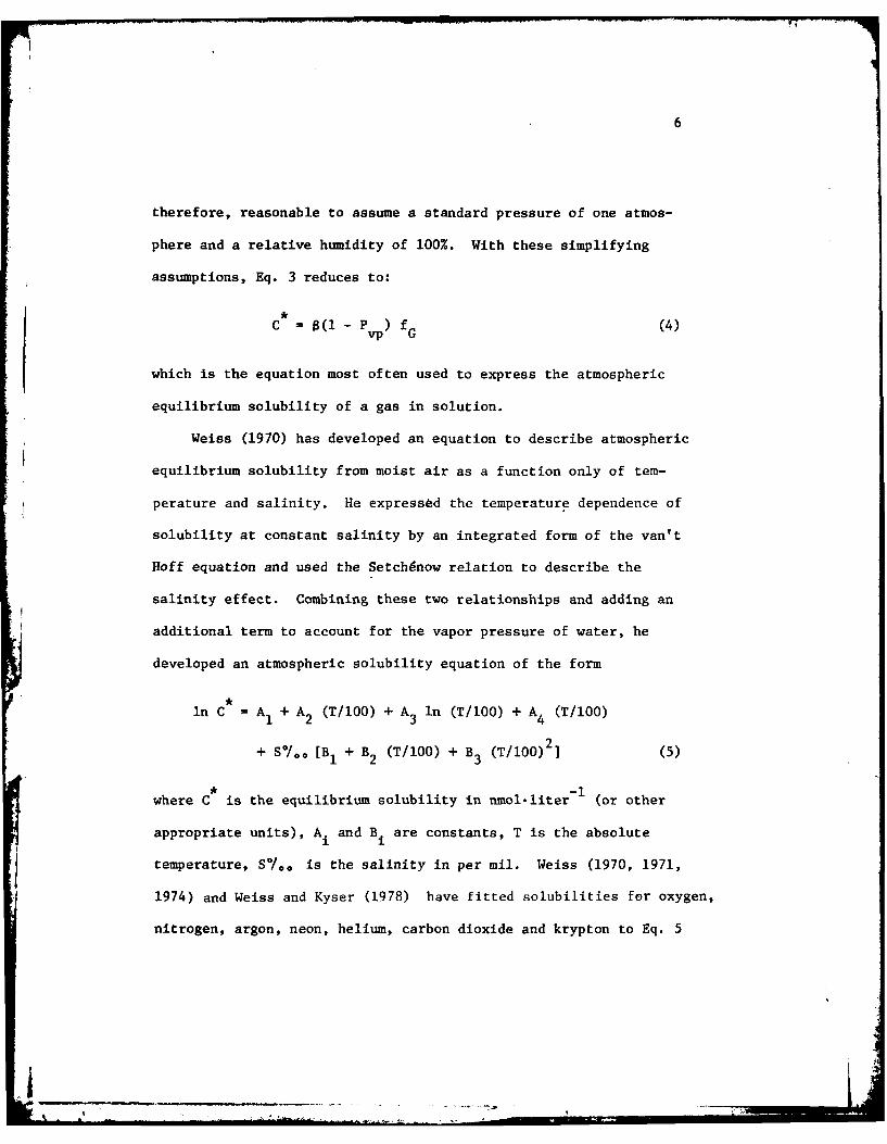
Weiss (1970) has developed an equation to describe atmospheric

equilibrium solubility from moist air as a function only of tem-

perature and salinity. He expressed the temperature dependence of

solubility at constant salinity by an integrated form of the van't

Hoff equation and used the Setch~now relation to describe the

salinity effect. Combining these two relationships and adding an

additional term to account for the vapor pressure of water, he

developed an atmospheric solubility equation of the form

in C = A1 + A2 (T/100) + A3 In (T/100) + A4 (T/100)

+ So/,. [BI + B2 (T/100) + B3 (T/100)2] (5)

where C is the equilibrium solubility in nmol.liter- 1 (or other

appropriate units), Ai and Bi are constants, T is the absolute

temperature, S0,'0 is the salinity in per mil. Weiss (1970, 1971,

1974) and Weiss and Kyser (1978) have fitted solubilities for oxygen,

nitrogen, argon, neon, helium, carbon dioxide and krypton to Eq. 5

7

to describe the atmospheric solubility of those gases relative to

water saturated air at one atmosphere total pressure. Recently,

Wiesenburg and Guinasso (1979) have rewritten Eq. 5 expanding the

A1 term to fg + A1 , to include the atmospheric gas concentration

as a variable. They have fitted solubility data for methane, hydro-

gen and carbon monoxide to the modified equation. All atmospheric

solubility calculations in this work will be made using Eq. 5 or

the modified version of Wiesenburg and Guinasso (1979).

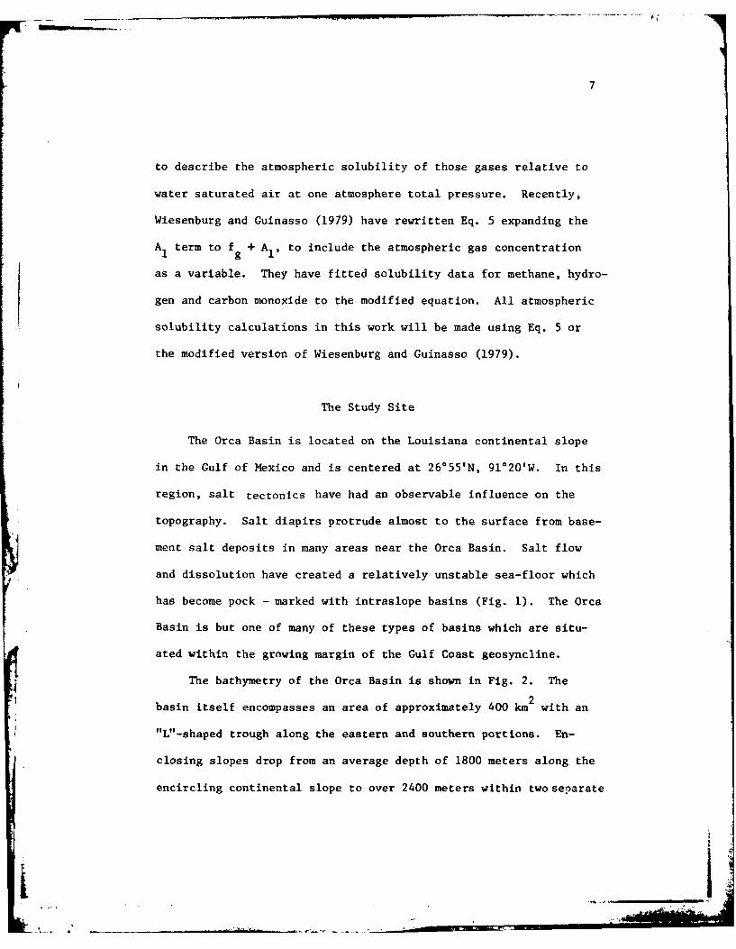
The Study Site

The Orca Basin is located on the Louisiana continental slope

in the Gulf of Mexico and is centered at 26*55'N, 91020'W. In this

region, salt tectonics have had an observable influence on the

topography. Salt diapirs protrude almost to the surface from base-

ment salt deposits in many areas near the Orca Basin. Salt flow

and dissolution have created a relatively unstable sea-floor which

has become pock - marked with intraslope basins (Fig. 1). The Orca

Basin is but one of many of these types of basins which are situ-

ated within the growing margin of the Gulf Coast geosyncline.

The bathymetry of the Orca Basin is shown in Fig. 2. The

basin itself encompasses an area of approximately 400 km2 with an

"L"-shaped trough along the eastern and southern portions. En-

closing slopes drop from an average depth of 1800 meters along the

encircling continental slope to over 2400 meters within two separate

IA

CL 00 "-40

-qo 0

N ccoN ca

9

27000'"'Xi

55-

55' iiiZ40o.S'

2650' - 950 900301, , , 1 , .. , ,.-

', w GULF OF MEXICO.,. -" ............ ,,............ i

OV& -2000m

.26oL . . . .

91025' 20' 91015 '

Fig. 2. Bathymetric map of the Orca Basin. based on theseismic data taken on cruise 76-G-10 of the R/V Gyre (afterShokes et al. 1977). The stippled portion of the map repre-sents the area covered by the high salinity brine.

10

areas. The bottom 200 meters of the Orca Basin is filled with

water having an evaporative salinity of 250*/.o and a temperature

(5.6*C) more than 1.4*C higher than the overlying, freely circula-

ting Gulf of Mexico water. The volume of brine in the Orca Basin is

3approximately 5 km , a volume several times larger than all of the

Red Sea brines combined.

The temperature and salinity structure in the Orca Basin is

shown in Fig. 3. Bottom water at 2000 meters in this area of the

Gulf of Mexico has a characteristic temperature of 4.2*C and an

average salinity of 34.976*/co. Both the temperature and salinity

begin to increase rapidly in the Orca Basin at a depth of approx-

imately 2240 meters, with the salinity gradient being more dramatic

than the temperature gradient. The sea water to brine transi-

tion zone from normal Gulf of Mexico deep water to maximum salinity

brine is only about 50 to 60 meters and provides a very sharp den-

sity contrast. The density difference of the brine (1.185 kg/i)

as compared to the deep Gulf water (1.025 kg/i) provides such a

sharp interface that it can be seen using low-frequency acoustical

sounding devices. Shokes et al. (1977) used a 700-joule minisparker

to generate low frequency sound pulses in order to map the

extent of the brine. Part of the record that they obtained in that

study is shown in Fig. 4. The brine appears as a distinct layer

due to the sound reflection from the interface. On cruise EN-32

of the R/V Endeavor, the brine interface could also be seen by

..

A|

11

TEMPERATURE (-C)

3.0 4.0 5.0 6.0 7.02000

60 ORCA BASINO71-G-10

2100 o

20N TEMPERATURE

400

100030

0.\

SNYSALINITY(i')

2300 -

2400 6

20 100 20 0

SALINITY (g.liter-1)

Fig. 3. Vertical temperature and salinity (g.liter - )profiles extending from the deep Gulf of Mexico water intothe hypersaline Orca Basin brine. Note the sharp transitionbetween the Gulf water (p = 1.025) and the brine (p 1.185kg. liter-1 ).

k ...

12

WATER DEPTH (METERS)

0 0 10 "' J-

TJ0

ci 0

r-1 0

I.- .

w-4'

cCO4L 4J

a) 0Ad

$4 E

,0 4-

00 W

4j -

r) 0 i10LI4 v 1

S 0)I ~t4 -4

0 0

0. 4.403S ~ ~ ~ ~ U 3 1-1A8 VMOJ

13

using a 3.5 kHz bottom profiling system, which has a higher fre-

quency than the minisparker of Shokes et al. (1977). This device

was instrumental in positioning the ship above the brine for sam-

pling. The brine-sea water interface could not be seen with the

higher frequency 12 kHz bottom profiling system.

Previous Investigations

The Early Work

The geochemical investigation of the Gyre Basin in the north-

western Gulf of Mexico (Bouma et al. 1975) prompted researchers at

Texas A&M University to perform surveys of several other intraslope

basins on the Texas and Louisiana continental slopes. Most of the

other intraslope basins appear to be geochemically "normal" basins

similar to the Gyre Basin (C. R. Schwab, personal communication).

Only the Orca Basin was found to have water with above normal

salinities.

The Orca Basin was first sampled as part of the intraslope

basin study during cruise 75-G-16 of the R/V Gyre in November 1975.

During this cruise, a 185-190 cm gravity core was taken from the

shoaler northern end of the basin (Fig. 2). After the core was

sliced and the interstitial water removed by squeezing, the water

(brine) was placed in a freezer but it would not freeze completely!

Examination of the interstitial fluid from this core revealed that

the salinity was greater than 250o/o. at a depth of 8 cm and

14

decreased slightly with depth in the core (McKee and Sidner 1976).

Although similar hypersaline conditions had been found in deep

borehole samples from the Gulf of Mexico (Manheim and Bischoff 1969),

this was the first observation of hypersaline fluids in any open

continental shelf or slope environment. With excitement running

high the brave men of the Gyre returned to the Orca Basin on cruise

76-G-2 in early 1976. A second gravity core was taken in the

deeper southern portion of the basin and water samples were taken

to characterize the water in the basin. They noted that the

basin had a local sill depth of 2000 m, with a 140 m thick bottom

layer of anoxic bottom water with a salinity of 270*'f. . The ob-

servations from these two cruises have been briefly summarized by

McKee and Sidner (1976). The first water column data (Table 2),

a description of the sediment features which result from the un-

usual environment was described. Since their observations are

relevant to all future studies, this author will briefly detail

them here:

1. The sediments are high in organic matter.

2. The presence of fine laminations reflect the lack of

burrowing organisms.

3. Sediments from the basin are black due to the presence of

metastable metal sulfides which rapidly oxidize to a red

brown color upon exposure to air.

1'15

Q)4 00 r- 0

I~-

0-

0

4-44

-H

$4 r-4

o0 4

e'4 Q~ Q,

$4

$0w

14

;LH4-4 CD00

+ + 0C'J 015 -4 4 j

-4 1-

16

4. There was no noticeable hydrogen sulfide odor in the water

or sediments.

5. The deeper water samples appeared gassy and the X-ray

radiographs of the cores showed small gas bubbles which

increased in concentration near the surface of the core.

6. The sediments show excellent organic preservation as

evidenced by the presence of Sargassum throughout the

entire length of the gravity cores.

These observations (McKee and Sidner 1976) were preliminary and

there were no interpretations of results given.

The first study to make detailed observations of the water

column chemistry was done by Shokes et al. (1977), using data ob-

tained during R/V Gyre cruise 76-G-10 in October 1976. This work

led to the landmark paper which first showed the extent of the

Orca Basin and gave it its name. Shokes et al. (1977) did a com-

plete bathymetric survey of the basin using a low frequency mini-

sparker and estimated the brine volume to be 40 km3 . They made

the first extensive geochemical analysis of the anoxic brine in the

Orca Basin. In this analysis, detailed vertical measurements of

temperature, salinity, oxygen, and nutrients were made in

both ends of the basin (Fig. 5 and 6). The major ions in the

brine were also measured and these values were compared to the

Red Sea geothermal brines (Table 3). Shokes et al. (1977) con-

cluded that the brine must originate by solution (presumably by

17

0 0-0 0 0 0

00 000r I

- ,0 CD 0

r- w- w- a

r-4 r-4 - n 0 I

U) o n nO

.0..a 0 I -. L 0D

U)0

*1r4

4

(U -L t LI -t m~

-40 0 .-

+4-4

U)4 000C~L~0

'00 C4 0% 14

tv4 0 '0 4 w p

0 4 ) 1 4 -

18

0 > al

C.,

00

(0 0 0- iipiLn - -c

00

0 X1

0-

-4 0

IT a) 0 )U

w~c w -0

j -CzO rDz $ 0ON4 LU m0 4) 0 r,

4U -Lu ,U') - w C r4

LU z c0 L 1<LU LU 0) 000 4 0 4D 0 10

0L - 0 o0- be'j 00

L)0

0i U)U)W4 mrz 0 0 C 1

000C~l - to 4

CI~u I v- d

0 0 -

0 0 I'

19

co

v0

0- 0- 0

0o 0 LA)I. 4

- l 0 0

0 0 co mU

0 00

00 0

0.4X

4J

0 0 0 0

r4-4

000 - 44O

0I 0 )

E 0 0

01

TI 03 -- o-,jO2;& .0--

0q W

0o0. 0 0

0 z 0 0 0 -

0se~w Hld]G r

20

sea water) of a near-surface salt deposit (mainly NaCI). They

reached this conclusion based on the absence of sulfate depletion

in the brine and due to observations of minimal changes in temper-

ature and ion compositions. Since there was a decreasing chloride

gradient in the interstitial water of the basin sediment, it was

suggested that the brine enters the basin laterally, rather than

by diffusion upwards through the underlying sediments. Calcula-

tions of the heat input needed to raise the temperature of the

40 km3 brine from the overlying Gulf temperature of 4.2C to the

present 5.6'C could be added in about 325 years, assuming an aver--2 -i)

age oceanic geothermal heat flow (1 ucal-cm *sec ). The only

dissolved gas measured was oxygen, which decreased to zero within

the brine.

In a follow-up paper, Trabant and Presley (1978) presented a

more detailed geological description of the Orca Basin. The brine

3volume estimate was lowered to 5 km . The geological setting of

the Orca Basin was compared to that of several other intraslope

basins which have been defined and discussed on the basis of

seismic reflection profiles (Antoine and Bryant 1969; Garrison

and Martin 1973). It was concluded that geologically the Orca

Basin represents a typical intraslope basin. However, it has

water with uncommon chemical composition and associated sediment

geochemistry because of the presence of regional salt massifs

which have led to salt flow into the brine. Trabant and Presley

21

(1978) examined a three meter gravity core taken in the deeper end

of the basin and came to the same conclusions as McKee and Sidner

(1976), viz. the absence of laminae and apparent textural homoge-

neity indicated pelagic deposition and no burrowing by organisms.

The presence of Sargassum throughout the core was also noted. A

complete description of the core was produced and the following

sediment properties were discussed:

1. The sediment was a silty clay with a clay size fraction

of 60-75%, with little or no vertical change of clay

mineralogy.

2. The acid-leachable iron content is similar to other Gulf

sediments, but with a relatively high sulfur content (1%)

compared to other Gulf of Mexico sediments.

3. Water content of the sediment ranged from 140% to 280%

(dry weight method).

In discussing the brine geochemistry in the Orca Basin, Tra-

bant and Presley (1978) make one significant new note. They

measured the bromide level in the brine and found a value of 80

mg-kg- . Due to the well-known partitioning effects associated

with bromine as a salt solution evaporates, bromine can be useful

in determining the origin of the brine (see later discussion on

bromine). LouAnn Salt (a logical source for salt in the Orca

Basin) was observed to have 34 to 51 ppm bromide (Holser 1966).

22

Dissolving 308 g of this salt in a liter of sea water would give a

bromide concentration equivalent to that found in the Orca Basin.

Thus, Trabant and Presley (1978) offered strong evidence that the

Orca Basin brine forms from the dissolution of previously deposited

salt.

In the same volume, a paper on basin and slope sediments by

McKee et al. (1978) further emphasized this point, while comparing

the sediment geochemistry of intraslope basins with the geochem-

istry of shelf and slope sediments. In this same study, they

noted that the more rapid sediment accumulation rate in intraslope

basins caused basin sediments to have a more anoxic character than

typical slope sediments. Of the basins studied, only the Orca

had brine in the bottom. However, one other basin - the Gyre

Basin - exhibited a higher concentration of salt in one of the

cores that were studied (up to 44.2 g-kg- 1 of chloride compared to

19.4 g-kg- 1 for average sea water). The salinity in this basin

core increased with depth in the sediment indicating an upward

diffusion of salt from some deeper formation.

Another significant feature of the study by McKee et al.

(1978) was a comparison of sulfate profiles of the normal slope

sediments, intraslope basin sediments, and the Orca Basin sediments.

Even though the sedimentation rate in the Orca Basin is three times

as great as found on the slope, the sulfate gradient from the

upper 120 cm of two Orca Basin cores was not significantly greater

23

than gradients found in most slope sediments. In one other Orca

Basin core (9B), the slope of the sulfate profile indicated a dc/dx o

of 0.27 mmol.liter- 1 cm which is higher than the value of 0.02- i -

mmol-liter-l, cm found outside the basin (but still lower than

some values found in the Gyre Basin which is not an anoxic basin).

The variability of sulfate gradients in the cores from the Gyre and

Orca Basins correlated with patterns of sediment redeposition within

the basins. More evidence of slumping was found in Gyre Basin

cores. However, those cores were more extensively studied than the

Orca Basin cores.

These initial studies on the Orca Basin were primarily con-

cerned with defining the origin of the brine. Two basic lines of

evidence were pursued: the decreasing chloride gradient in the

sediments and the bulk ion composition. The decreasing salt con-

centration with depth in the sediments is strong support for the

salt influx coming from other than the basin floor. However, the

ion composition is also an important piece of evidence in decipher-

ing this puzzle. The ionic composition of the Orca Basin brine as

reported by Shokes et al. (1977) is compared with standard sea

water and several other oceanic brines in Table 3. Unlike evap-

oration brines such as the Dead Sea brine, the Orca Basin brine

does not have tremendously increased concentrations of any

ions other than sodium and chloride. This fact, and more recent

evaluation of bromide data from the Orca Basin by McKee et al.

24

(1978), both support the contention that the Orca Basin formed as

the result of the dissolution of a salt deposit. The bromide con-

cept is important enough to describe in more detail.

Bromide does not form its own minerals when sea water evapo-

rates. Some of it is lost from solution because it forms isomor-

phous admixture with chloride in the precipitates (Valyashko 1956;

Braitsch and Herrman 1963). As sea water evaporates, the carbon-

ates precipitate first, followed by the sulfates. During this

stage of evaporation, little or no bromide precipitates, or if it

does, it is occluded with the carbonates and sulfates (see Table 4).

Halite (NaCl) begins to precipitate when the chloride concen-

tration reaches about 275,000 mg-liter (cf. normal sea water,

19,000 mg-liter- ). Some small amount of bromide is entrained with

chloride in the precipitate. However, as crystallization proceeds,

more bromide is left in solution than is included in the precipi-

tate. Sylvite (KCI) begins to precipitate when the chloride con-

centration has risen to about 360,000 mgliter-I. Carnallite (Mg

CI2 KCI-6H20) and bischoffite (MgCl2"6H20) precipitates follow.

During evaporation the concentration of bromide in solution in-

creases. Therefore, relative to chloride, the bromide concentra-

tion in a brine is a good indicator of the degree of sea water

concentration. The above discussion assumes that appreciable

quantities of biogenic bromide have not been introduced into the

system. McKee et al. (1978) have discussed this idea and

4

25

0.C4 -.1 00 1-- 0 W) 0 0 0'.0 cn 0 C14 0 00 0 0 0

-0C4 ,-4 1-4 0~0Lo~ 0' 0- 0 ,0 0 0 0 0

0

0~ 00 -I 00 00 00 co 0p* C'14 0 0 "-4 0 in 0 0D 00 ~0 0D 0 N- 0D 1.0 0D

4-4 '.0 0; 0; C

C, 4 C) 0 o C' 4 0 D D

-. 1 C 0 0 C) 0 0 H- 000 CD CD

0 £*' CD ~ m.L 0 0 n CD

U00 H: -: C;1r-Cn 00U

8-i

-4 0 0a - 0 0C04 J.J 0 .i4 "40.40.0 01 4 C C 1. U C I . 0 H

CUc 0 mC .4 C *-It CU U 0 0 "4

0I ~ U C14 L -4 E-

kc

26

illustrated it with a diagram (reproduced here as Fig. 7) that shows

bromide versus chlorinity for various pore waters including the

Orca Basin. As sea water evaporates, the chloride versus bromine

distribution is represented by the solid line which separates the

areas resulting from dissolving, evaporate-produced brine from

residual source-solution brines. The Orca Basin is higher in

chloride content without a significant increase in the bromide

concentration indicating a solution source. This data seems to

clearly establish the source of the Orca Basin as a dissolving

evaporite deposit rather than a brine formed by direct evaporation.

Subsequent Investigations

These papers caused a flurry of activity in the oceanographic

community. Besides cruises-by Texas A&M University, expeditions

to the Orca Basin have been staged by the University of Miami, the

University of Texas and the University of Rhode Island. In the

Fall 1977 American Geophysical Union meeting, seven papers were

presented dealing with various geochemical aspects of the Orca

Basin (see, for example, Guinasso 1977).

Of the papers now published from the initial cruises to the

basin, I recognize two major categories: sediment geology and

organic-microbial interactions in the brine. The sediment papers

have been produced by geologists searching for the source of salt

or are attempting to describe the unusual effects that the high

27

0

-,j ) cU)

14 to a) mW 0 A '-H cc

wcuq

0 D w >

W Q) 0 to.0 - U)a04

ui CL 4Q )

cr w 0 30 ( 4- Cukwz

-4~0-

W u 0 0

0 0 m>

UJEo A- C 0 V

C CO M U H HcoW 44- w

CC

>o)- - 4 co >

(L.J~!r. AIINUO1H

28

salinity water has on various sediment properties (e.g., sedimen-

tation rate, clay particle interaction, and preservation of carbon-

ate and silicious materials). Kennett and Penrose (1978) used

electron microscopy to examine the microfauna in the sediments.

They noted that pteropod tests were extremely well preserved rela-

tive to other areas. Additionally, they noted the unusual occur-

rence of well preserved Sargassum particles deep in the core.

While Sargassum has been found at the sediment surfaces as deep as

5300 m (Schoener and Row 1970), Kennett and Penrose (1978) noted

that there are no previously documented cases of preserved seaweed

in deep-sea sediments, especially with attached organisms as found

in the Orca Basin.

Addy and Behrens (1980) also reported the presence of seaweed

in their ten meter core from the knoll between two basins. They

did a very complete study of the major ions in the interstitial

water and for each 10 cm section of the core, determined grain

size distributions. From radiocarbon dates, they determined that

the bottom layer of the black mud in the sediments (which corre-

sponds to the initial time of brine input to the basin) had an age

of 7910 + 170 years. This age was reported at a depth of 4.85

meters which gave an implied sedimentation rate of 61 cm-ka-1

Measurements further down in the core in areas which were not

deposited under anoxic (brine) conditions gave a sedimentation

rate for that region of 43 cm-ka - . This difference implies an

29

increased sediment accumulation rate due to the anoxic conditions

existing in the brine. Carbonate percentages averaged four percent

higher in the black mud laid down under anoxic conditions than in

the gray mud that had an oxygenated origin. From this data, Addy

and Behrens (1980) concluded that the enhanced sediment accumula-

tion is due to increased preservation of carbonate test. The

higher sand fractions in the basin core were almost entirely skele-

tal carbonate.

Besides the color of the mud in the sediments, Addy and Beh-

rens (1980) used the presence of Sargassum fronds to ascertain the

conditions (anoxic or aerobic) under which the sediments were de-

posited. Aerobic conditions allow more degradation of organic

matter than in anoxic environments. The absence of recognizable

Sargassum in Orca Basin gray muds indicates deposition in an oxy-

genated environment; while the well preserved Sargassum fronds in

the black mud strongly suggest deposition in anoxic brine.

Addy and Behrens (1980) made several other measurements to

determine the conditions of deposition, including water content

(higher in the anoxic mud) and compaction (found to be less in the

black mud sediments). Deposition in a brine basin would account

for both of these observations.

The color of the black mud is due to very fine-grained, meta-

stable iron sulfides such as greigite (Fe3S4) and machinawite

(FeS), like those found in anoxic sediments of the Black Sea

30

(Berner 1974). Formation of metastable iron sulfides instead of

pyrite (FeS2) will result in the absence of significant H2S (from

So4 reduction) in the depositional environment. This observation

has important implications for the work to be presented later.

Addy and Behrens (1980) approached the questions of brine

origin by conducting seismic profiles of the slope area. If the

Orca Basin brine is formed from dissolution of an exposed salt dia-

pir, that feature should be found on the surrounding basin slope.

In two multichannel subbottom profiles, Addy and Behrens (1980)

noted several strong undulating reflectors with diapiric structures

which they interpreted as salt surfaces. These salt surfaces be-

come shallower to the north and possibly outcrop at the edge of

the small basin east of the Orca Basin. A second salt structure

similarly approaches the surface at the eastern margin north of

the Orca Basin. A 3.5 kHz profile of the region showed hyperbolic

reflections indicating a hummocky surface. Addy and Behrens noted

that if salt were exposed, the dissolution would proceed along

fractures and joints resulting in the uneven surfaces that were

observed. Perhaps Addy and Behrens (1980) have located the source

of the Orca Basin brine.

Another study dealing with sediment geology was that of Tomp-

kins and Shephard (1979). They described possible depositional

processes, geotechnical properties and clay mineralogy of two

cores from the Orca Basin. One core was taken in the deepest

31

portion of the southern basin and gave sedimentation rates of over

100 cm-ka 1, based on microfaunal examinations. The conditions

within the core suggested that the sediment was originally depos-

ited under brine on the basin slope, and then slumped deeper

into the basin. Addy and Behrens (1980) had avoided problems re-

lated to slumping by sampling only on the knoll between the two

basins.

Tompkins and Shephard (1979) examined the clay mineralogy

and clay mineral variations in the basin sediments. They noted

an increase in smectite with increasing depth (and decreasing

salt) in the sediments. They attributed the highly open sediment

microstructure to the rapid sedimentation. Both the sediment micro-

structure and the levels of smectite seemed to control the diver-

sity in clay mineral abundances in the brine. Sediments that were

deposited outside the brine, then slumped into the basin, were

easily discernable by their properties which were similar to normal

continental slope sediments.

In a study which encompassed both water column and sediment

data, Sackett et al. (1979) developed a carbon budget for the Orca

Basin water column and sediments. Methane and carbon dioxide

increased with depth in the sediments and both were assumed to

result from the bacterial decomposition of organic matter. The

81l3C values of carbon dioxide and methane in the sediments were

very negative (isotopically lighter) relative to water column

1", ,*

32

values. The value of -105o/.. that Sackett et al. (1979) observed

for the 61 3C of methane is the lightest (natural) methane isotope

ratio reported to date. The amounts of organic carbon found in the

sediments were somewhat higher than for normal shelf and slope

sediments. The 613C values of the particulate organic carbon in

the sediments ranged from -22*o/. (a normal value for open shelf

sediments) down to a -26.7*o/e They suggested that the lighter

samples may have resulted from slumped material originally depos-

ited in estuarine environments during the Pleistocene.

In the brine itself, Sackett et al. (1979) made concentration

and isotopic (613C) measurements of carbon dioxide, methane, and

organic carbon. Sackett et al. (1979) used a mass balance equation

of the following form:

,[(mg C/L)(613C)]sea + [(mg C/L)(613C)]ae* L 'flg ~ 'sea water '~"''added carbon

[(mg C/L)(61 3C)]brine (6)

to calculate the amount of isotopic composition of added carbon

that would be required (starting from sea water) to produce the

values for methane and carbon dioxide they observed in the brine

and sediments. These calculations revealed that the carbon added

to the Orca Basin had a concentration of 27.4 mgC-liter- I with a

613C of -33Y.° . Sackett et al. (1979) were also able to partition

the 27.4 mgC liter- 1 between carbon dioxide added directly (via

33

fermentation) and carbon dioxide that had been cycled through an

anaerobic methane consumption pathway (CH4-) CO2). Their estimates

from these contributions were 26.3 mgC-liter- I from interstitial

total carbon dioxide and 26.3 mgC-liter- of carbon dioxide from

methane oxidation. They suggested that the observed isotopic ratios

of carbon can be explained by some complex mixture of three bac-

terially catalyzed processes: carbon dioxide fermentation, acetate

fermentation, and sulfide reduction (encompassing methane consump-

tion).

Realizing the importance of bacteria in an anoxic environment

such as the Orca Basin, LaRock et al. (1979) examined bacterial

activity in the brine. Total biomass was measured in both the

deep Gulf water and in the brine using direct counts of bacteria,

ATP levels, and uridine uptake. ATP concentration and uridine

uptake both decreased just below the interface and then increased

with increasing depth. This pattern was similar to the ATP dis-

tribution in the Cariaco Trench (Karl et al. 1977). In the deepest

sample from the brine an ATP value of 15.4 ng liter was found.

This high level indicates that an active microbial population has

developed within the brine of the Orca Basin.

The most interesting pattern shown by the microbial data was

at the brine/sea water interface. Both ATP levels and uridine

uptake values displayed similar patterns in the interface region.

They increased in magnitude (relative to deep Gulf levels) above

34

the interface but decreased below the interface in the anoxic zone.

This pattern, showing the existence of an interface population (or

ATP subsurface maximum) at the brine/sea water interface, is con-

sistent with the concept of particles resting on the density gradi-

ent. Bacteria and particles are closely associated in the deep

ocean and conditions at the interface are well suited to the de-

velopment of an autotrophic bacterial population. The anoxic zone

provides a source of both nutrients and other energy yielding

* substrates (by diffusion upward from the brine) and could pro-

vide a rich medium for bacterial reproduction.

Ignoring the decomposition processes that had intrigued most

other workers, Millero, et al. (1979) concentrated on the physical-

chemical properties of the brine. They measured conductivity,

density, and the speed of sound in the brine and in various brine

dilutions. The speed of sound in the brine is 16% greater in the

brine than in sea water with a salinity of 350/oo . This finding

allows us to calculate the depth of the basin. The high sound

velocity implies that the basin is deeper, and thus larger, than

previously estimated by Shokes et al. (1977).

Millero et al. (1979) also found that salinity and density

(under standard conditions) were consistent within the anoxic zone

of the basin. These density and salinity measurements were done

with exceptional care and corroborated the earlier data of Shokes

et al. (1977). Millero et al. (1979) used the density measurements

35

to examine the physlo-chemical nature of the brine. The ionic

composition of the brine was used in additivity methods (of partial

and molal volumes) to estimate the density of the brine. Measured

values agreed with these estimates to within t 280 x 10-6 g.cm-3 ,

from 150 to 350C. Since this agreement was good, Millero et al.

(1979) suggested that it seemed possible to make additional esti-

mates of physio-chemical properties of brines using additivity

methods.

Anaerobic Decomposition Processes

The salt that has flowed into the depths of the Orca Basin

has created a large density gradient as was discussed earlier.

Table 5 presents a list of various basins, both oxygen-bearing and

anoxic, along with the stability of the water column in each basin.

The hypersalinity in the Orca Basin has given the water in the

basin water a stability that is nine orders of magnitude greater

than the major anoxic basins in the ocean.

The stability of the Orca Basin has produced an isolated sys-

tem removed from the general circulation of the oceans which

provide renewal waters to other areas. With an absence of fresh,

oxygenated water flowing into this geochemical system, oxygen

becomes depleted and anaerobic decomposition processes begin.

Little if any flushing can occur across its density gradient. The

extreme stability of the Orca Basin thus makes it an ideal

.......

36

Table 5. Approximate stability across the sills of some basinsand fjords (after Richards 1965).

BASIN AOT/AZ x 10-3 m- 1

OXYGEN-BEARING BASINS

Gulf of Mexico 2 x 10- 6

Catalina Basin 3.1 x 10-6

Santa Barbara Basin 4.4 x 10- 6

Santa Monica Basin 8.8 x 10- 6

ANOXIC BASINS

Kaoe Bay 2.4 x 10 - 5

Cariaco Trench 3.2 x 10- 5

Gulf of Cariaco 3.5 x 10- 5

Saanich Inlet 1.5 x 10 - 5

Black Sea 3.0 x 10 - 4

* +3Orca Basin

3.2 x 10

Calculated from data of Shokes et al. (1977).

-

37

laboratory for examining the mechanisms of anaerobic decomposition.

An understanding of anaerobic decomposition processes is im-

portant to marine geochemists. The sequence of oxygen depletion,

followed by nitrate, nitrite, and sulfate reduction is an oft

repeated pattern in anoxic marine basins and fjords (Richards 1965),

evaporite basins (Borchert and Muir 1964), and during the early

diagenesis of marine sediments (see, for example, Martens et al.

1978). Many marine sediments are anoxic, especially along contin-

ental margins where the sedimentation rate is high. Such sediments

receive a large flux of organic matter, its origin being the fixa-

tion of organic carbon in the overlying photosynthetic zone. Or-

ganic-rich sediments undergo early diagenesis in which microorga-

nisms consume the labile organic matter using first oxygen, then

nitrate, nitrite, and sulfate as oxidizers until each is depleted

and methanogenesis takes place. The products of this anaerobic

decomposition diffuse out of the sediments into the overlying sea

water.

Early diagenesis in sediments overlain by oxygenated waters

cannot be interpreted by examining reduced species concentration

in the overlying waters. Diagenetic products diffusing out of

the sediment into oxygenated sea water are diluted or are consumed

by oxidizing bacteria. The oxidation products in each case are

compounds (e.g., CO2) that are in large abundances or are rapidly

diluted in aerobic sea water. It thus becomes difficult to assess

a

38

their input into the overlying water and consequently their geo-

chemical impact on the oceans. For sediments at the bottom of

anoxic basins or fjords, however, there is no free oxygen available

to act as an oxidant to alter the decomposition products.

Thus the terminal products of anaerobic decomposition accumulate in

the overlying anoxic waters.

Such anoxic basins and fjords provide scientists with natural

laboratories for examining the geochemistry and microbiology of

organic matter decomposition. The Black Sea, being the largest

anoxic basin in the world, has received the most attention. After

the results of the 1967 U.S. expedition had been reported (Degens

and Ross 1974), Laking (1974) compiled a bibliography with over

4,000 citations of research- in the Black Sea. Since Richards (1955)

reported the discovery of anoxic sea water in the Cariaco Trench,

there have been over 120 papers published on this isolated Vene-

zuelan basin (for a review, see Richards 1975). Such intense

research activity is but another example of the scientific interest

in anoxic environments. This interest is well justified. The

chemical changes that led to the development of anoxic conditions

are of interest beyond the immediate confines of the stagnating

waters in basins and fjords where they are studied.

Examinations of regenerated nutrients and dissolved gases in

anoxic environments has led to various models which explain the

anaerobic decomposition of organic matter. During anaerobic

* .,I-,

39

decomposition, organic material [represented here as (CH20)106

(NH3 )16H3PO4 1 is decomposed into the nutrient H3P04, and thedissolved gases CO2 , CH4 , NH3 % N2 , and H 2S. To describe this pro-

cess, simple stoichiometric reactions have been used with some

success (Richards et al. 1965; Gaines and Pilson 1972; Adams 1973).

An example is the reaction of Richards (1965) for phosphorus and

nitrogen liberation during bacterial sulfate reduction.

(CH20)1 06 (NH3)1 6H3P04 + 53S0-4

106C02 + 53S + 16NH3 + H 3PO4 + 106H2 0 (7)

The C:N:P ratio of organic matter in this reaction is the average

value of plankton of 106:16:1 given by Redfield (1934) and Fleming

(1940).

Richards' model has been applied to the Cariaco Trench, Black

Sea, Lake Nitinat, and Saanich Inlet. Most of these anoxic envi-

ronments experience either periodic mass flushing or a slow

continual input of oxygenated water into the anoxic waters. Unless

the magnitude and time scale of the flushing can be accurately

estimated for each area, it becomes difficult to apply the model.

This is true since dissolved oxygen enters with renewal water.

Input of oxygen can result in removal (oxidation) of reduced com-

pounds and inhibition of anaerobic bacteria. With the discovery

of the anoxic, hypersaline Orca Basin in the Gulf of Mexico (McKee

wmta -

!I

40

and Sidner 1976; Shokes et al. 1977) we have discovered a new

natural laboratory to study anaerobic decomposition processes. As

we shall see, this is a laboratory which does not experience the

mass periodic or even slow gradual flushings of other anoxic basins.

Research Objectives

The unusual circumstances involved in the formation and chem-

istry of the Orca Basin make it a desirable area for oceanographic

research. It is an unusual system when compared to the normal

distributions of major ions and gases in the ocean. However, it

probably is not unique when viewed in a geological perspective.

Basins similar in nature to the hypersaline Orca Basin must have

been common in the geological history of the Mediterranean Sea and

other regions where salt tectonics has played an important role

(N. L. Guinasso, personal communication). Remnants of basins

similar to Orca Basin (as evidenced by rapid sedimentation rate)

are found buried in the deeper sediments below the Mediterranean.

Understanding such basins may be important on a geological time

scale. Understanding decomposition processes is important on a

daily basis. Dissolved gases can be useful geochemical tracers

in such an environment. Inert gases can be used to elucidate

formation processes, while biogenic gases (major products of

anaerobic decomposition) yield information about current reactive

processes.

~-~-- ~..

41

Most of the published work on the Orca Basin has ignored the

dissolved gases in the basin. Shokes et al. (1977) noted that

gases effervesced from the water (brine) when it was brought to

the surface, but they made no measurements of the effluent gases.

Only dissolved oxygen, which decreases to zero in the brine, was

measured. In their carbon budget study, Sackett et al. (1979)

measured both methane and carbon dioxide of the basin water and

sediments. Their approach was to concentrate on the carbon com-

pounds in the basin. Sackett et al. (1979) did not consider all

the dissolved gases resulting from anaerobic decomposition.

In examining the hot, salty Red Sea brines, Craig (1969)

pointed out that dissolved gas distributions could be a powerful

tool in evaluating the mechanisms of brine formation. This is

true since, unlike the major ions, initial gas concentrations are

independent of both the ion ratios of the brine and the bulk ion

composition of the salt from which the brine formed. Weiss (1969) used

nitrogen, argon, and carbon dioxide values from the Red Sea brine

to gain valuable information concerning its source of origin. He

showed the utility of dissolved gas measurements in such unusual

environments. With these ideas in mind, this author has undertaken

a systematic study of the dissolved gases in the Orca Basin. The

objective of this study has been to use dissolved gases to address

some of the questions relevant to both the Orca Basin and to

anaerobic decompositions in general.

42

These questions include:

1. What is the source of the Orca Basin brine and can dis-

solved gas data be used to confirm the source?

2. How is anaerobic decomposition of organic material affected

by high salinity water?

3. What are the origin and significance of the isotopically

light methane in the brine and sediments of the Orca

Basin?

4. Why is there no hydrogen sulfide in the Orca Basin in

spite of evidence of sulfate reduction in the sediments?

5. What role does the input of biogenic carbon dioxide gas

play in the carbonate chemistry of the brine?

43

CHAPTER II

DENSITY EFFECTS AND PHYSICAL MIXING PROCESSES

Introduction

The dissolved gas distributions in the Orca Basin are directly

affected by the density gradient and interface mixing processes

which result from the presence of brine in the bottom of the basin.

Thus, a consideration of the physical characteristics of the Orca

Basin brine is important to this study. The Gulf of Mexico sea

water above the Orca Basin exhibits temperature and salinity depth

profiles (Fig. 8) which are typical of the expected distributions

in this area of the western Gulf (cf. Nowlin 1972). Below about

2000 m, however, the salinity concentrations begin to increase

slowly until an extremely rapid increase in temperature and salt

content are observed at about 2250 m (see Fig. 3). Salinity in-

creases from about 70*O/. to over 250*/oo over a depth interval of

only 17 m. This rapidly changing salinity has produced the dis-

tinct pycnocline at this level.

A true appreciation of the significance of the pycnocline in

the Orca Basin can be obtained by comparing the density gradient

in the Orca Basin with the pycnocline near the surface of the Gulf

of Mexico (Fig. 9). The surface pycnocline separates the homog-

enous mixed layer from the bulk of the oceans and it is this

pycnocline which is responsible for maintaining the nutrient and

. . ... ..........

44

TEMPERATURE (°C)

0 4 8 12 16 20 24 28

Tenipeature -.. -

"0

500 0 ""-----, Salinity

E#

CL]UiU

U)U

E 1000 "

w

3.0 3

Gulf of Mexico78-6-2

1500 Sta. 4-3

0

2000 o

34.0 34.5 35.0 35.5 36.0 36.5

SALINITY (%o)

Fig. 8. Typical temperature and salinity depth pro-files taken in the water column of the northwestern Gulfof Mexico above the Orca Basin.

45

DENSITY (kg-liter')

1025 1050 1075 1/00 1/25 1/50 1175 12000 ~ r F T r T-- F

400

Gulf of Mexico

800

E1-/200

I-O-w

1600

2000

Orca Basin2400

Fig. 9. Density profile for the Gulf of Mexico, extend-

ing down through the Orca Basin brine. Density at the brine

interface increases from 1.025 to 1.185 kg-liter-I over a

depth interval of less than 50 meters. This is one of the

most striking density gradients of an oceanic area (see

Table 5).

46

biological distributions in surface waters. That surface pycnocline

is dwarfed by the density gradient at the surface of the Orca Basin

brine layer. It is this gradient that reflects the low frequency

sound waves that can be recorded even. at a frequency as high as

3.5 kHz.

The Orca Basin pycnocline must act as a temporary trap for

many of the particles which fall into the Basin. As particles

settle through the water column, most have a density only slightly

greater than the water through which they fall. Upon reaching the

density gradient above the Orca Basin, their downward progress will

be impeded. These particles probably stop at the density interface

and begin to soak up salts (or dehydrate due to osmosis) until

they reach isotonic balance with the brine. This may not be a

continuous process. Particles may have to go through several

layers or steps before their density will have increased suffi-

ciently to allow them to proceed on their journey to the sediments.

Even at the sediment interface, particles do not have a sufficient

density, relative to the encompassing brine, to compact completely

at first. As a result, the surface sediments are soupy, and they

are difficult to sample since they tend to run out of the smallest

hole in a box corer or other sampling device.

Support for the concept of an increased particle abundance at

the brine-sea water interface comes from the bacterial biomass

data of LaRock et al. (1979). They observed an increase in both

47

adenosine triphosphate levels and total bacterial cell counts in

samples taken from the Orca Basin interface, as opposed to samples

taken from the brine or from waters above the interface. Bacteria

in the deep ocean are usually attached to particles rather than

free-floating. Thus higher microbial biomass at the interface

would be indicative of an increased particle density at that level.

This increased microbial biomass was consistent with findings from

another stratified basin, the Cariaco Trench, where Karl et al.

(1977) observed a similar ATP distribution. The degree of strat-

ification in the Orca Basin can be discerned by a detailed exami-

nation of the temperature and salinity distributions through the

interface.

Temperature Distribution

Examination of a continuous temperature profile through the

interface to the bottom of the Orca Basin (Fig. 10) with a Plessy

Environmental Model 9040 STD shows that the Orca Basin brine is

not thermally homogenous. Temperature begins to increase at a

depth of around 2150 meters. The temperature depth profile goes

through several steps between 2150 and 2250 meters before a more

rapid increase begins. In the highest salinity brine (>2500o/.),

there are at least two distinct layers having a temperature dif-

ference of about 0.05*C. This two-layer system within the brine

was not observed by Shokes et al. (1977), who used reversing

48

Wt6c

14 WbCv

co 0

:3 000 0-4.J,

z. as4 0C~ >a

ix CO

w~~ U) vqs-4 0.

-4 0 w

ccw .Ij -4 -4

toccE/

-> 4.1

'IH ~44 W

0 M4 4w

01C0o4

49

deep-sea thermometers to obtain their temperature profile.

Temperature of the Orca Basin sediment was measured (acci-

dently) on cruise 77-G-3 of the R/V Gyre when the same STD used to

make the profile in Fig. 10 was lowered into the mud. Due to the

small density difference between brine and sediment particles

falling into the basin, the top layer of sediment in the Orca Basin

is very soft and unconsolidated, with about the same consistency

as clam chowder (New England style). The surface sediments have a

temperature of 5.77*C, a value 0.03*C higher than the bottom water

temperature. This temperature differential between the brine and the

sediment indicates that the brine is heated from below and would

account for the heat flow required to raise the initial brine temper-

ature from the original 4.2*C (Deep Gulf water) to the 5.6%C found

today. Heat flow calculations and comparison with the estimates of

Shokes et al. (1977) are given in a later section.

Salinity Distribution

The importance of the density gradient which results from

brine in the bottom of the basin was discussed in Chapter One.

This density gradient (Fig. 9) is dependent not on temperature,

but salinity. The temperature of the high salinity (>35*/..) water

increases with depth (Fig. 10). A temperature increase would

result in a corresponding density decrease without the effect of

50

salt on density. Since salt is the major factor influencing den-

sity, salinity can be equated with density for the following dis-

cussion.

The salinity depth distribution in the Orca Basin falls log-

ically into three zones. I have classified these zones (proceeding

from deep to shallow) as the high salinity brine, the interface

zone and the transition zone (Fig. 11). The high salinity brine is

a semihomogenous mixture (Millero et al. 1979) with a salinity

of 262*/.., relative to standard sea water. The brine, which

occupies the bottom 200 m of the Orca Basin, appears to have two

thermal layers (Fig. 10) with a slightly higher temperature in the

deeper region. This thermal gradient makes the lower layer slightly

unstable with respect to the upper layer of the brine and thus

could cause it to mix (see mixing discussion). The high salinity

brine is very stable, however, relative to the water above it.

The interface above the high salinity brine is the most marked

salinity gradient in the basin. Salinity increases from 701. to

over 260/.. with a depth decrease of only 17 m. This change

(dS/dz = 11.5 ,-m - 1 ) is an order of magnitude greater than the

zone either above or below it. It was very difficult to obtain

samples in this region. The points plotted on Fig. 11 were ob-

tained using the STD-rosette sampling system that was used to

produce Fig. 10. The data points that were plotted (Table 6) re-

veal the narrow range of depths involved. Data were taken from

51

SALINI[Y (%o)

2100 40 80 120 160 200 240 280

21200

2140

2160 TI

" 2180.

E' T22200-

0 2220-T3

2 2 4 0 -' - -.?4 calp Interface Zone

Change 70

2250"

2260 2F2 .

2270 High Salinity Brine

2280 - 1 1 1 1 1 1

Fig. 11. Detailed vertical profile of salinity throughthe interface region of the Orca Basin. Three zones areidentified: the transition zone from Gulf water, the trueinterface zone where salinities increase from 70 to 2620/ oand the high salinity brine with a constant salinity of262o/... The transition zone is subdivided into threeregions depending on the change in slope of salinity anddissolved oxygen concentrations with depth (see Table 6).

-. - .tA. 31.-.L.. -. -

52

Table 6. Temperatures and salinities taken from two STD casts oncruise 77-G-13. Note the large change in salinity over such a smalldepth.

Depth Temp Salinity* Cast(meters) (C) (/.)

2204 4.26 46 4

2230 4.54 60 4

2240 4.63 66 4

2248 4.77 138 4

2248 4.72 150 9

2250 4.81 176 9

2252 4.88 199 9

2256 4.96 238 4

2257 5.15 256 9

2268 5.38 266 9

. Salinity samples were volume diluted to a salinity near 35gokg-1

and analyzed using standard Copenhagen Water as a reference. Vol- 1

umes were converted to weights using a brine density of 1.185g.kg

53

two separate casts using the same system, yet samples from identical

depths of 2248 mn from each cast show a salinity difference of

12 0/00 (138 cf. 150 */. Table 6).

The interface zone probably results from a mixing of the high

salinity brine below with the transition zone water above. The

lower layer of the transition zone (T3) has a salinity at the bottom

of 70 0100. A two point mixing curve for the interface zone would

have 70 *lee and 262 0/00 as the end points (Fig. 11). The two point

mixing model seems to fit the salinity data in Fig. 11 reasonably

well. Linear regression analysis of the data produces a straight line

with a coefficient of variation of 0.991. Salinity changes by one

part per thousand for each nine cm. in this zone.

An STD system was the only reliable device capable of taking

numerous samples in this narrow region on a single cast. The paucity

of data from this region in other papers (e.g., LaRock et al. 1979)

shows how difficult it is to obtain samples there. When closely

spaced additional salinity samples are obtained, the two point mixing

curve for this interface zone can be used to accurately calculate

sample position relative to the high salinity brine.

The transition zone can be classified into three regions.

The characteristics of each region are listed in Table 7. The

upper region (TI) is the area where density first begins to in-

crease from the constant values of the deep Gulf water. The

-~ -- -VA

54

Table 7. Salinity zones in and above the Orca Basin.

Zone Region Salinity Depth as 02 3O2Range Range Z -l Range as(7.) (W) (0/..m Xuaol- -1 ) (nolL - 1 0/..)

Transition Ti 35.2 2130 0.031 225 30.5

37.0 2178 170

Transition T2 37.0 2178 0.42 170 12.3

50.0 2209 10

Transition T3 50.0 2209 0.62 10 0.5

70.0 2241 0

Interface I 70.0 2241 11.53 0

262.0 2258

High SalinityBrine B 262.0 2258 0 0

+0.2 2430 ,(bottom)

Exact bottom of Orca Basin varies.

A

55

salinity change is small, but the effects are apparent. The depth

of this region is about 50 meters. Transition region T2 spans a

depth interval of 31 m with a dS/dz of 0.42, an order or magnitude

greater than the region above. The salinity at the bottom of this

region is 500/00. The deepest transition region has a salinity of

between 50 and 70*O./ Salinity in this region increases about 1.5

times as fast as in the region above. Region T3 abutts the

interface zone below. It is in this region (T3) that Shokes et al.

(1977) observed the step in the oxygen profile.

An examination of the temperature profile in the basin (Fig.

9) indicates that each salinity region is associated with a dif-

ferent slope in the temperature gradient. It is of interest to

note here, that the slope of zone T3 for temperature is not much

less than the thermal slope for the interface zone. Salinity

changes, on the other hand, represent an order of magnitude in-

crease in slope between region T3 and the interface zone.

The salinity distribution in the high salinity brine (Fig. 3)

shows no obvious differences with depth. These data were obtained

by volume dilutions of the brine before analysis by conductive

salinometry (Shokes et al. 1977). Millero et al. (1979) performed

precise weight dilutions on six samples from the brine and found

an average salinity of 262.84 + 0.14*/... The bottom samples had

an average of 263.02*o/. (a = 0.03) and the four above then aver-

aged 262.75/.. (a = 0.02). This slight difference gives an

56

indication of a two-layered salinity distribution. The difference

in the means of these two levels is significant at the 95% confi-

dence level, but only six samples were compared. More detailed

salinity sampling is necessary to precisely define the salinity

layering in the brine.

An attempt to obtain a detailed salinity profile was made on

Gyre cruise 78-G-2. The Plessey 9040 STD was modified to simul-

taneously measure temperature and salinity in the high salinity

brine. This STD has a normal salinity range of only 30-40 0/00.

In more saline waters, the salinity output frequency overlaps into

the temperature frequency range, obscuring both the temperature and

salinity measurements. To measure salinity, a nylon plug was placed

in the center of the salinity-sensing induction toroid. Insertion

of this plug, with a 0.95 cm diameter hole drilled through its

center, reduced the effective cross-sectional area of the toroid,

The area was reduced sufficiently to make the measured inductance of

the high salinity water the same as the inductance of 37 */.8 sea

water in an unmodified STD, while not interfering with the

temperature measurements.

The modified STD was lowered into the deepest portion of the

basin on March 28, 1978. The rough untreated data from this

attempt is shown in Fig. 12, along with an expansion of the tem-

perature trace in the high salinity brine. The salinity profile

shows a slight increase, with depth to the bottom, with two zones

having separate slopes. The observed change in slope of the

-L-e

57

V4

E--

00cl-4

0?- zCD z .6 1Io

6,m

C--d.. cc00

LN C .l0 i

V

LjJ V)

(k) .-H

Vo -r4

w 00

40

-4 V-4

0

22502275 2300 2325 2350 2375 24b0 2425 2450 247S00>

DEPTH1 (METERS)

e4 X.141

4.

58

salinity profile, however, does not occur where the temperature

profile shows an increase. Thus the continuous data do not indicate

that there are two separate layers with homogeneous temperature and

alinity. It must be remembered that the validity of this salinity

trace has to be questioned. The technique that was used to produce

the salinity profiles is rather unorthodox, and no calibrations

were made to determine the true salinities. The flushing volumes

of the smaller toroid also require investigation. The data does

indicate, however, that a detailed examination of the salinity

structure in the Orca Basin would be profitable in interpreting

water structures in the basin.

Mixing Procesies in the Orca Basin

High Salinity Brine

In spite of the above discussion, the salinity distribution

in the high salinity brine is considered to be essentially uni-

form. This homogeneity is also true for several other parameters

that have been reported for the high salinity brine (see, for

example, Sackett et al. 1979). It follows that some mixing must

be taking place to create this homogeneous mixture in the brine.

There are several possible mechanisms for mixing. One mechanism

would be mixing due to input of new brine. Other possibilities

would be mixing resulting from thermal processes in the high

salinity waters or from seiching the brine.

59

New brine entering into the depths of the basin would mix until

there was a re-establishment of the density structure in the brine.

This mixing process would be rapid however, and would probably

result in mixing of the brine such that both temperature and salin-

ity were well mixed. As can be seen in Figs. 10 and 12, temperature

is not thermally homogeneous in the brine. Thus, a slower mixing

process must be invoked to account for the thermal layers, as well

as the homogeneous salinity and other parameters.

Such a process might be convective mixing due to heating from

below. This mechanism could only account for mixing in the high

salinity brine where the salinity content is approximately constant

at 262*/... The temperature differences in this high salinity

brine are about 0.050C between the two layers and could not support

density imbalances with a significant salinity gradient. Thus the

following discussion of possible convective overturn processes in

the Orca Basin is applicable only to the high salinity brine. This

is the 262*/.. brine in the bottom 140 m of the basin and not the

lower salinity waters in the interface or transition zones that

were described earlier.

It is quite possible that mixing in the basin deeps is driven

by convective overturn resulting from the increasing temperature

with depth in the high salinity brine. The bottom temperature

measurement with the STD indicated that the Orca Basin is being

heated from below. The bottom sediments are 0.03*C warmer than

60

the brine. The deep Gulf of Mexico water is l.4*C cooler than the

high salinity brine. The Orca Basin high salinity brine is similar

to the classical thermal convection situation where there is heat-

driven motion in a layer of fluid (the brine) contained between

two horizontal planes, uniformly heated from below (the sediment)

and cooled from above (Gulf water). In this type of system, deeper

water becomes less dense than the water above it, due to increased

heating from below, and can mix upward. Apparently, convective

overturn is not uncommon in closed basins which are isolated from

the more rapid advective mixing processes. For example, Newman

(1976) examined the water structure in Lake Kivu and applied the

same type of analysis to that system. Like the Orca Basin, he

noted steps in the temperature profile in Lake Kivu and attributed

the associated mixing in the lake to double-diffusive convective

mixing. Turner (1968) also noted that there is increasing evi-

dence that a step-like structure is characteristic of the ocean

and some lakes. Instead of smooth gradients in temperature and

salinity, well mixed layers separated by sharp interfaces are

often observed. The layers would be the result of convective

mixing of the waters due to heating from below. The same type of

mixing may explain the homogeneity of salinity and other parameters

in the high salinity brine of the Orca Basin.

The problem of convective overturn due to differential heat-

ing has been well studied in the realm of fluid mechanics. Benard

61

(1901) first showed that a thin layer of fluid becomes unstable

when the temperature (i.e., density) differences exceeds a minimum

value. Fluid motion takes place in a regular, steady pattern at

first, but can become turbulent with large temperature differences.

As described by Turner (1973), an unstable fluid layer of thickness

6 is driven upward (z direction) by buoyancy forces (density

differences) but retarded by viscosity, and neglecting inertial

effects there is a local imbalance. Unless the driving forces are

much greater than the dissipative forces, the system will remain

stable, in spite of the instability of a particular individual

layer. The mathematics of the instability was first formulated and

solved by Lord Rayleigh (Turner 1973). He showed that there is a

critical value of Ra, the non-dimensional Rayleigh number, below

which a fluid heated from below is stable to small disturbances.

The Rayleigh number, Ra, is given as

Ra = (ga/-y) ATh 3 (8)

where

g is acceleration due to gravity

a is the thermal coefficient of expansion

K is the thermal conductivity

y is the kinematic viscosity

AT is the temperature difference across a layer

h is the thickness of the layer

62

The Rayleigh number represents the balance between the driving

buoyancy forces and the diffusive processes which retard the

motion and tend to stabilize it. At.a value of Ra of 10 3to 104

cells which fill the gap between boundaries become unstable and

convective overturn can occur (Turner 1968, 1965).

Since fluid mechanicians usually deal with pure fluids (i.e.,

distilled water), the above description is normally applied to

systems that only have a temperature gradient to cause the density

imbalance. In the oceanic environment, however, there is usually

a salinity gradient to consider also in interpreting buoyancy

forces available to initiate convective overturn. The problem of

convective overturn in linearly stratified salt solutions has been

examined by Turner and Stommel (1964) and others. Turner and

Stomel (1964) gave a qualitative description of the motions that

result when a linearly stratified salt solution is heated uniformly

from below. That description was clearly summarized by Turner

(1968) and it could be used to describe the mixing regime in the

high salinity brine of the Orca Basin. Rather than attempt to

improve on his description, I simply quote:

Convective stirring first produces a layer at the bottomof the containing vessel which is well mixed in bothheat and salt, and which grows by incorporating fluidfrom above. This layer does not continue to deepen in-definitely, however: at some point a second layer formson top of it, and this behaves in the same way. In time,many such layers can form, with sharp interfaces sepa-rating the turbulent convecting regions, and these inter-faces stay in nearly fixed positions until the bottom

63

one disappears as the lowest two layers merge. Thesystem can be maintained in this state because of thevery different molecular diffusivities of heat andsalt: heat can more easily escape from the top of alayer to cause a convective overturning above, whilethe salt mostly stays behind and preserves a netstable density difference across the interface(Turner 1968).

The question to be considered here is whether heat input from

the sediments into the Orca Basin brine is sufficient to create

the density imbalance required to exceed the critical Rayleigh

numlber, Ra . Unfortunately, various parameters such as the

viscosity and thermal conductivity have not been determined for the

Orca Basin brine. Thus in order to calculate Ra using Eq. 8, 1

have chosen the values for the thermal coefficient of expansion,

thermal conductivity and kinematic viscosity that Newman (1976)

used for Lake Kivu. The values for sea water would be equally

applicable, since these terms are not the dominant terms in the

equation. Increases in salinity tend to cause both the viscosity

and the thermal coefficient of expansion to increase.

The two combined increases tend to cancel since the ratio

of the two is used in Eq. 8. Using Newman's (1976) data and the

4 Orca Basin values of O.05*C difference between the two layers

with an interface distance of 25 m between the high salinity brine

layers, a Rayleigh number on the order of 10 13was calculated.

This value is several orders of magnitude larger than the critical

4value of Ra - 10 Based on this calculation, it seems reasonable

64

to assume that the layering observed in the high salinity brine of

the Orca Basin is due to double-diffusive convective mixing driven

by geothermal heating from the basin sediments. Conclusive proof

of this hypothesis requires a more sophisticated set of constants

for the Rayleigh number calculation, as well as a better definition

of the salinity and temperature microstructure in the high salinity

brine.

Oxygen Step Region and General Mixing

One of the most striking features of the data presented by

Shokes et al. (1977) was the anomaly (step) just above the high

salinity brine in the oxygen depth profile. A comparison of the

oxygen data (Fig. 5) and the temperature and salinity profiles

(Figs. 10 and 11) indicates that the oxygen step is associated

with one of the physical layers in the brine transition zone,

region T3. There are many complex forces acting upon this inter-

face region. Salinity increases from 50*/oe to 70*/.o. Tempera-

ture increases from 4.250 C to 4.75*C. The brine interface may

be oscillating with time. This region could be physically active.

There are two plausible explanations for this step region. Either

new, oxygenated brine is being put in at this level, or oxygenated

water from above is mixing with water from the interface zone

below to create this higher salinity,oxygenated water in region

T3.

65

An examination of a temperature versus salinity plot for the

Orca Basin is helpful in understanding the processes acting on the

oxygen step region. Fig. 13 is a plot of the temperature and

salinity data from Fig. 3. The salinity data are given in units of

g-liter -1, since the samples were volume diluted. Correcting

the data for density and replotting in salinity units of g-kg1l

showed the same profiles, and would not alter the data interpre-

tations. Fig. 13a shows a plot of all the temperature and salinity

data taken from depths of 2050 m down to 2430 m, near the bottom of

the basin. The solid line drawn through the data follows the data

from a salinity of 35 0/oo to a salinity of 170 0/00, and then the

second half of the curve (from 170 to 305 */.,) is simply a mirror

image of the left hand portion of the solid curve. The curve was

drawn in this manner since this data set (after Shokes et al. 1977)

had only two data points in the high salinity region, other than in

the high salinity brine itself. Fig. 13b is an expansion of the

data between 35 and 70 9/o from Fig. 13a, indicated by the area

between arrows on Fig. 13a. The T-S profile in this region is

almost a straight line, which is indicative of a two point mixing

condition. The two points representing the extremes of the straight

line drawn on Fig. 13b would be the temperatures and salinities of

the two water masses that are mixing.

Fig. 13c is an expansion of the data between 45 and 75 /.

and also exhibits the same straight line structure indicative of

66

6.0

EXPANDED 2430

, 52 -

4.8 5

4.4 -

40 j I L L I I0 50 100 150 200 250 300 350

50 -EXPA14DED BELOW

w 48i

,46

CcIUjU

S 4.4

w4.2

B40 I I I

30 40 50 60 to 80

48

47

46

4.5

U C4.4 I

45 50 55 60 65 70 75

SALINITY (g.liter')

Fig. 13. Salinity versus temperatureprofile for the Orca Basin. Parts b and care expanded plots of the data presented inpart a. The data are taken from the samedata shown in Fig. 3.

67

a two-point mixing model. Most of the points on Fig. 13c are

from the oxygen step region shown on Fig. 5.

If the water in the oxygen step region is the result of a two

point mixing process, this could explain the oxygen concentrations

found in that zone. The oxygen would be oxygen mixed downward from

above. This mixing, however, is probably not due to convective

overturn as was discussed in the previous section for the high

salinity brine. Salinity increases from 50 0/00 at the top of zone

T3, to 70 0/00 at the bottom, 32 m below. For this zone to turn

over due to heating from below, the 70 */.. salinity water would

have to reach a temperature of over 55*C. There is no evidence

for such high temperatures at the Orca Basin interface. Yet,

evidence for mixing of the oxygen step region(T3) is compelling.

The salinity-temperature plots presented in Fig. 13 might be

explained by diffusive mixing processes alone, if one assumes that

a double diffusive process is taking place. That is temperature

and salinity are diffusing at different rates. For molecular

diffusion, this is indeed the situation. Heat diffuses faster

than salt (Hunk 1966). Two questions to be considered in this

discussion are what are the differences in the diffusion rates of

these two parameters at the Orea Basin interface, and how does

~1 diffusivity change with distance from the interface.

If one assumes that the brine flowed without mixing into the

depths of the Orca Basin at some initial time t - 0, then at that

68

time the brine was covered by Gulf of Mexico water with a sharp

boundary between the two. In fluid dynamics, this initial case is

described as one in which the distribution occupies a finite

region with an initial state defined by:

C=Cos Z <0, C =0, Z >0, at t 0 (9)

where C =concentration, Z = distance, t = time and Z =0 at the

interface. This distribution is analogous to one in which a long

tube of clear water rests on a long column of solution, or when a

long water column of Gulf of Mexico water rests on top of the Orca

Basin brine. The case for the Orca Basin is shown diagramatically

in Fig. 14. At a time toll both the temperature and salinity pro-

files have only one value in the Gulf water (T.1, S 1) and a single

value in the brine (T 2 S 2). The profile at time t1I is illustra-

ted by the solid line in Fig. 14.

After initial diffusive mixing, the Orca Basin interface must

reach steady-state to be maintained. This can be proved by performing

a simple calculation of how long the temperature profile would be

maintained at a constant thermal diffusivity of 103 cm 2.sec-1

Using the simple relationship,

L = Dt (10)

where L is length, D is the thermal diffusivity, and t is time, one

can calculate the characteristic time for diffusion to spread an

initial temperature step function. The interface thickness is

1700 cm. With D T = 10 -3, the time required for diffusivity to

spread an initial step function to the present thickness is

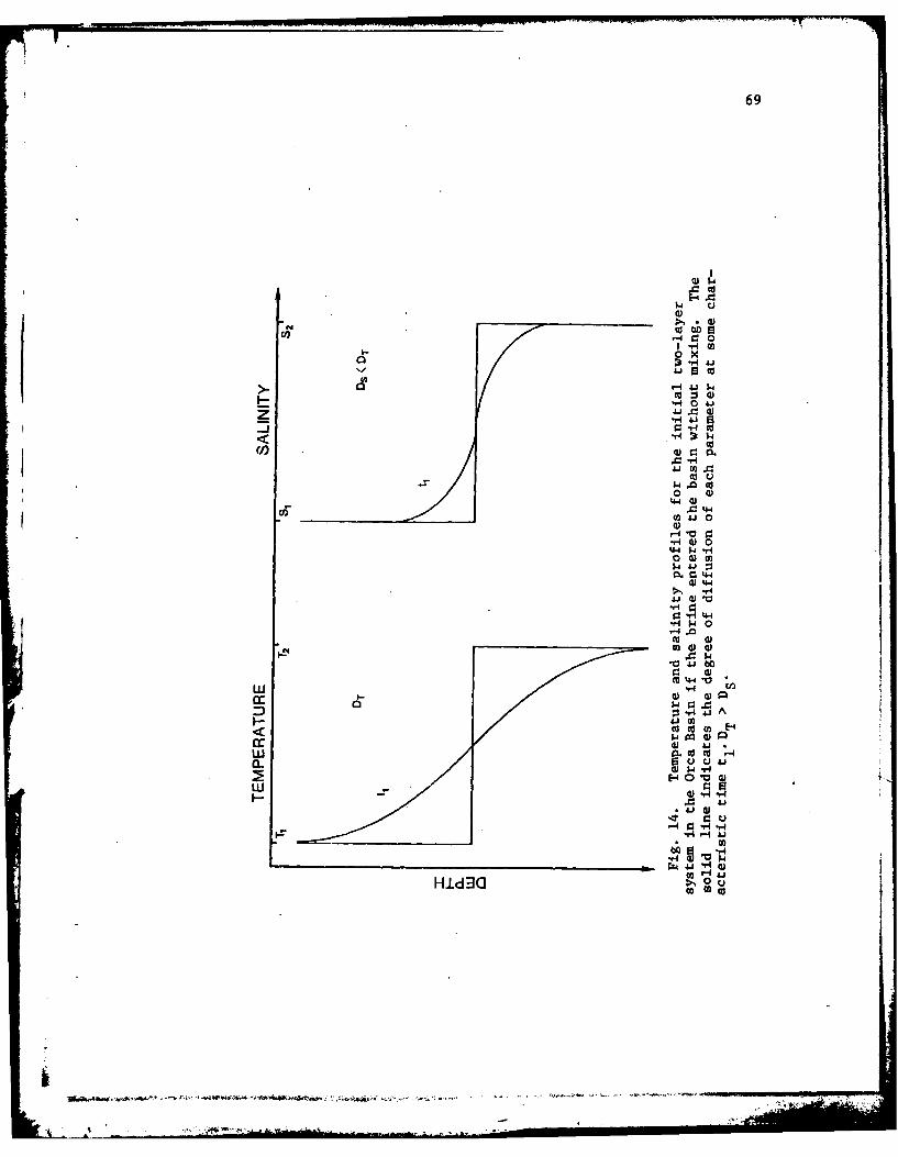
69

0 C

a I -4 4J .

a ~.,-a J

00

4) 044 $4 -H

0

r.J 4-1

w 0

041

0 4-a, '.-

D0 A

ir* 4 J 00LU .to C _1

w 9-4 r4P 0 0

LL0

[Aid3J0

0002 E12

70

2.9 x 10O9 sec, or about 90 years. Since the time of initial input

of brine into the Orca Basin is -8000 years, time dependent pro-

cesses would have removed the interface long ago. Similarly, time-

dependent diffusion of salt (D. 10 )would spread the salinity

11interface in 3x 10 sec, or about 9000 years. The Orca Basin

interface region would be unstable unless the system were steady-

state.

A comparison of the STD temperature-depth profiles in the

basin taken during three different years supports the steady-state

concept. The first temperature-depth profile with an STD system

was taken in 1977 by Guinasso (1977). The latest profile was taken

in March, 1980, on Gyre cruise 80-G-4. The thermal layers through-

out the basin (Fig. 15) are Identical in both profiles, yet geo-

thermal heat is entering the brine from below. This input would

change the temperature interface without a balanced output. The

Orca Basin diffusion must be in steady-state relative to heat.

Salt diffusion would not be steady-state without an input,

but diffusion out would be very slow. Assuming a diffusion co-

efficient for salt of 10cm. sec , one can calculate the time

for all salt in the basin to diffuse out. A one cm. column in the

deepest part of the basin would contain 2 x 10 5cm 3 of brine, with

each cm. containing 0.25 g of salt. With D S 10-5, a salt flux of

-10 -2 -11.25 x 10 g-cm *sec is calculated. Dividing the mass of salt

in hewaer olmn(5 1 4g-cm -2) by the flux gives 4 x 10 13sec,

or about 1,300,000 years, as the time for all the salt to diffuse

out of the basin. In the 8000 years since the brine entered the

71

1.4

4)-4

0 C0

Id0LIJ

L4JJ

(0 0~

a:- -v C

w. 0 41

0j 0

1.4 0

0 0"

&4 41

13(44

0

72

basin, only 0.6% of the salt could have diffused out. The saie

would be true for other solutes produced there. Transport of

solutes frcm the brine to the overlying Gulf waters would be very slow.

The slope of the twelve thermal layers in Fig. 15 can be used

to calculate changes in thermal diffusivity. Through the interface

(layer 5) diffusion must be entirely molecular. With such a large

temperature and salinity increase over the short distance (17 m)

of this zone, processes more rapid than molecular would rapidly

distort the interface. With only molecular diffusion, the trans-

port of heat through the interface is due only to the thermal

conductivity of the brine. The average salinity in layer 5 is 167 /o.

A 17% NaCl solution would have a thermal conductivity of 1.345 x

10-3 cal-cm- -sec- l . C -1 (Weast 1969). The temperature change

across the 1700 cm interface is 0.65*C, giving a slope, dT/dz, of

3.76 x 10 -4.oCcm - . Heat flux through the interface (layer 5)

can be calculated by the formula:

Heat Flux = K (11)

dz

where K is the thermal conductivity. Heat flux through the inter-

-2 -lface was calculated as 0.5 Vcal-cm .sec . This flux is half of

the world average geothermal heat flow used by Shokes et al. (1977)

to calculate the time to heat the brine to 5.6*C. Since the Orca

Basin brine is in approximate geothermal balance, their estimate

is probably too high for this area.

If heat transport in the Orca Basin is steady-state, the heat

flux through any layer in Fig. 15 will be the same. The heat flux

through layer 5 has been calculated. Thus, using the slope of each

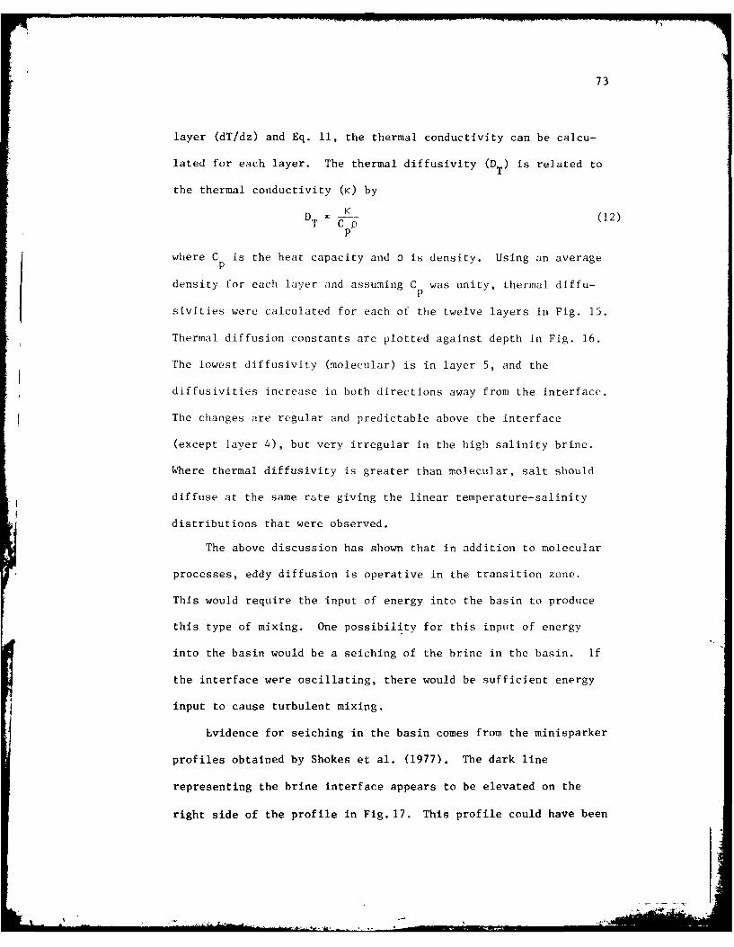
73

layer (dT/dz) and Eq. 11, the thermal conductivity can be calcu-

lated for each layer. The thermal diffusivity (DT) is related to

the thermal conductivity (K) by

D K (12)DT CpP

where C is the heat capacity and p is density. Using an averagep

density for each layer and assuming C was unity, thermal diffu-p

sivities were calculated for each of the twelve layers in Fig. 15.

Thermal diffusion constants are plotted against depth in Fig. 16.

The lowest diffusivity (molecular) is in layer 5, and the

diffusivities increase in both directions away from the interface.

The changes are regular and predictable above the interface

(except layer 4), but very irregular in the high salinity brine.

Where thermal diffusivity is greater than molecular, salt should

diffuse at the same rate giving the linear temperature-salinity

distributions that were observed.

The above discussion has shown that in addition to molecular

processes, eddy diffusion is operative in the transition zone.

This would require the input of energy into the basin to produce

this type of mixing. One possibility for this input of energy

into the basin would be a seiching of the brine in the basin. If

the interface were oscillating, there would be sufficient energy

input to cause turbulent mixing.

Evidence for seiching in the basin comes from the minisparker

profiles obtained by Shokes et al. (1977). The dark line

representing the brine interface appears to be elevated on the

right side of the profile in Fig. 17. This profile could have been

74

0 ~ ~ ~ ~ ~ ~ ~ ~ ~ 4 M__ _ _ _ _ _ _ _ _ _ _ _ _ _ _ _ _o a I J IH

IE4

* *r4n

I4. 0

41

.4

I 0

Ir*r

44 p. 0

.-4 4J 4'4P4 0)

CJl CV) o 0-H1

ClY(~ew HidCj ~j cmN

75

(UI r-.

- 4 -

I . 4

77=* Ta

'. ADA1OS 536 TEKXAS A AND N UNMIV COLLEGE STATION DEPT OF OCEANOGRAPHY F/0 8/4.GEOCHEMISTRY OF DISSOLVED OASES IN THE NYPERSALINE ORCA BASIN. (IJDEC 80 D A WIESENSIJRO NOOO475..C-0537

UNCLASSIFIED TAN -RE-801-T M

~3Mh~~hEEhhEEEEEMM hEEEE

76

taken when the interface was tilted due to seiching. Examination

of several other of the minisparker records from cruise 76-G-10

showed that several transects exhibited a tilt in the interface.

One of the profiles examined is shown in Fig. 17. The right

hand side of this profile, which was taken along the longest

section of the big basin is slightly higher than the left hand

side of the profile. Energy to induce seiching could result from

internal waves or even storms passing over with a reduction in

barometric pressure. Merrell (1971) has calculated that

energy from passing storms can influence bottom currents several

thousand meters below.

When seiching occurs in the basin, turbulent mixing will

occur on both sides of the brine sea water interface (layer 5).

This is identical to the case in fluid mechanics of oscillations of

the common boundary of two superimposed liquids. The motion will

be damped more quickly than seiches in lakes since the low density

contrast has the effect of diminishing the velocity of propa-

gation of waves of any given length in the ratio [(l-s)/(l+s)] /2 ,

where s is the ratio of the density of the Gulf water to that of the

brine (0.88).

In oscillations of a water mass with two layers, there will be

a discontinuity of motion at the interface. Fig. 18 shows mixing

processes as a result of seiching in a two layer system with arrow

vectors indicating the magnitude and direction of the water

movements. The normal velocities are continuous, but the tangential

77

Ti

3T

4-

_ _ _ ___ _ _

T-

of~~ a4 comlet osiltin hdphi

exggrae (afte Neuman an iesn 96

wig 18.i sclations of aheihe in-lyee

system).

78

velocity changes direction as the interface is crossed (Lamb 1945).

With the mixing at the interface, it is possible that the

oxygenated water from above would mix with the brine from below and

produce the oxygen step region that was observed. The diffusivities

above the brine (Fig. 16) should be high enough to allow mixing ofI oxygen downward into this region.

79

CHAPTER III

MAJOR ATMOSPHERIC GASES IN THE

ORCA BASIN BRINE

Of the twelve atmospheric gases listed in Table 1, only nitro-

gen, oxygen and argon have concentrations of about one percent (Ar)

or larger (N2, 02). These major, atmospheric gases have been

measured in many oceanic environments. Their high atmospheric

concentration results in dissolved levels in sea water which are

great enough to be measured by simple gas chromatographic tech-

niques. Oxygen is by far the most important gas in the ocean. It

is required by all marine animals for survival and is produced

during primary production by the phytoplankton in the surface

oceans. In deeper waters, oxygen is consumed more rapidly than it

is produced. The term apparent oxygen utilization (A.O.U.) has

been defined (Redfield 1934) as the amount of oxygen removed due

to respiration processes.

Argon and nitrogen are generally regarded as nonreactive in

ocean waters. Some qualification of this assumption may be nec-

essary for nitrogen, since it has been shown to be produced in the

anoxic waters of the Cariaco Trench (Richards and Benson 1961;

Linnenbom and Swinnerton 1969) and in some anoxic sediments (Wilson

1978). The oceanic distribution of argon and nitrogen is deter-

mined by physical mixing processes and by the effects of temper-

ature and salinity on their solubility. In contrast, the

, . t~~-- -

80

distribution of oxygen is influenced by biological as well as

physical properties. Thus measurements of unreactive gases, along

with oxygen, are useful in obtaining a quantitative separation

of the effects of physical and biological processes on the distri-

bution of oxygen in the ocean.

As was discussed in detail in Chapter I, the atmospheric

equilibrium of dissolved gases in sea water is a function of both

the temperature and salinity. The atmospheric equilibrium solu-

bilities of oxygen, nitrogen and argon in sea water at 351.o.

salinity are given in Table 8. These values were calculated from

Eq. 5, using the constants determined by Weiss (1970). A plot

of temperature versus solubility for argon and nitrogen (Fig. 19)

shows that the relationship is not a linear one. This concept is

important in interpreting the gas solubility data from a particular

area, since the mixing of two water masses with the same salinity

and different temperatures would produce an apparent supersatura-

tion. For example, if two waters of 35Yoo salinity, one having a

temperature of 0OC and the other at 30*C, the apparent supersatur-

ation would range from 7.8% for nitrogen to 8.6% for argon (Fig.

19).

In studying the major atmospheric gases in the Orca Basin, I

have examined both the concentrations and the solubilities of the

gases in the brine. A major purpose of these measurements is to

determine whether or not there has been dissolved nitrogen

i]

81

Table 8. Solubilities of N2, 02, Ar in sea water at 35*'/.salinity based on Eq. 5 and coefficients from Weiss (1970).

Solubilities (umol'kg' I)toc N2 02 Ar

0 616.3 349.5 16.98

5 549.6 309.1 15.01

10 495.6 274.8 13.42

15 451.3 247.7 12.11

20 414.4 225.2 11.03

25 383.4 206.3 10.11

30 356.8 190.3 9.33

A

82

V L)

w0 1

0 0 0 0 0 0 0 0 oi-0n 0 tin 0 0 U) 0 041 4CD C if) LOl CIT

0j

/~$ "4s./ V4 UIc ~ 41~/4 '~cs

r4 b . to

4 o u .4~ o

0 C 45 C

W -r 4-

83

production in the brine. It will be observed that both nitrogen

and argon are supersaturated in the brine relative to the brine

temperature and salinity at one atmosphere total pressure. This

chapter addresses the question of the origin of nitrogen and argon

in the brine and what one can learn from these unreactive gases

concerning the origin and geochemistry of the Orca Basin.

Methods

Gas Solubilities

Since gas solubilities had not been previously measured in

hypersaline waters, there was a need to determine whether or not

actual measured solubilities deviated significantly from the ex-

trapolated data obtained using the equations of Weiss (1970). To

equilibrate the brine with gases, a glass, thermally-regulated

equilibration chamber was constructed using a design similar to

one used by Schmidt (1979) for measuring atmospheric solubilities

of hydrogen and carbon monoxide (Fig. 20). Into this chamber,

approximately 400 ml of brine (or sea water for comparison) was

introduced and gas was bubbled through at a rate of 40 ml-min1l

for 30 min. The time required to saturate the brine with the

equilibration gas should follow a simple first order exponential

decay curve, assuming that equilibrium is reached between the

bubbles in the equilibration gas and the bubbles in the stripper.

84

PLATINUMGAS VENTRESISTANCE

THERMOMETER

COOLANTOUT

. PURGINGCYLINDER

STOPCOCK

COOLANT IN-

STANDARDGAS INLET

Fig. 20. Schematic diagram of thermal jacketedpurge cylinder used to equilibrate the brine withdissolved gases.

85

The characteristic time required to increase the concentration of

the gas i in solution by a factor of l/e is given by

ti ii~l (13)1 F4-

where B is the Bunsen solubility coefficient of the gas i at the

temperature of the liquid, V Iis the volume of the liquid, F+ is

the volume rate of flow of i in the equilibration gas at STP, and

P is the partial pressure of i inside the equilibration chamber, in

atmospheres (1 atm = 101.325 kPa). To make this calculation,

Bunsen coefficients were calculated for each gas, and other values

(e.g. flow rate) were measured. At 00C the characteristic time

required to equilibrate sea water at 20*C was 15 sec for oxygen,

17 sec for argon and 8 sec for nitrogen. For each of the brine

and sea water measurements, the equilibration gas was allowed to

flow for a period of 30 min to assure that complete equilibration

was reached. Air was used for the nitrogen source gas yielding

atmospheric equilibrated values. Pure (>99.995%) argon and methane

were used to measure Bunsen coefficients for those gases.

Since the bubbling of a gas through a liquid may tend to

supersaturate the liquid with the gas used, one further precaution

was taken during these measurements. After the 30 min equilibra-

tion period, the equilibration gas was shut off and the system

sealed with one atmosphere of gas above the sample for two min

before the brine was sampled. Analysis of the dissolved gas was

86

accomplished using the same gas chromatographic techniques as were

used for Orca Basin samples (see below). As an additional check on

possible supersaturation, sea water samples of a known salinity

were analyzed using the same procedures as for the brine. Sinceif the equilibrium solubilities of dissolved gases in sea water of

normal salinity are known very precisely as a function of tempera-

ture and salinity, these measurements served as external standards

for the equilibrium process.

The temperature of the brine in the equilibrator was monitored

using a thin film platinum resistance electrode which was epoxy

coated and immersed in the brine during the equilibration process.

This probe was calibrated against the high precision platinum

electrode (Leeds and Northrup, SIN 1762254) used to calibrate the

Texas A&M University reversing deep-sea thermometers. The high

precision probe is calibrated periodically against NBS temperature

standards. The temperature measurements in this equilibration

study are accurate to + O.02*C.

Dissolved OxygenI Dissolved oxygen was measured on the sea water samples wecollected from the Orca Basin by the microWinkler method of

Carpenter (1965). No oxygen was found in the high salinity brine

so no problems due to effervescing of the brine were observed here.

Nor was the degassing effect noted in samples taken from the

87

interface where small amounts of oxygen had been previously mea-

sured (Shokes et al. 1977). As discussed previously, Shokes et al.

(1977) had found an unusual step-like feature in the oxygen profile

just above the brine interface, with values constant at about 0.1

ml-liter - . After Wiesenburg et al. (1977) reported finding high

nitrite concentrations in the interface area of the Basin, the

standard Winkler technique was modified by adding one gram of

sodium azide to the NaOH-NaI reagent. Any nitrite in a Winkler

oxygen sample will reduce iodide to iodine just as oxygen does,

thus erroneously causing a larger value to be reported. Adding

sodium azide to the alkaline iodide reagent will prevent this

nitrite interference (Broenkow and Cline 1969).

Argon and Nitrogen Sampling

Samples obtained from the Orca Basin brine for argon and ni-

trogen are supersaturated with these gases when sampled at one

atmosphere total pressure. Since these gases will bubble out of

the water during sampling, special precautions had to be taken to

avoid both atmospheric contamination and loss of gas due to effer-

vescence of the samples. A system was devised to capture the

water sample before degassing took place.

A major problem with brine degassing was related to the type

of sample bottles used. All plastic Niskin sampling bottles are

the preferred water sampling device for marine geochemists. They

88

provide large volumes of water, are relatively inert and are trace

metal free. These bottles, however, have a closing device comprised

of a rubber band between two end caps. The pressure on the seal

is minimal at best, and could not keep the Orca Basin gases from

effervescing in the sample bottle, before they could be transferred

to some suitable sample container. Sampling with teflon-coated,

brass, 1.2 liter Nansen bottles proved more fruitful. These bottles

have a metal, ball-valve type sealing system which closes off both

ends of the bottle with a metal-to-metal seal when the bottle is

tripped. The seal produced by these bottles was tight enough to

prevent gas effervescence before transfer from the Nansen bottle.

However, using Nansen bottles, there was more variability between

samples in the brine than can be accounted for by analytical error

(assuming the brine is a homogenous mixture) so some of the Nansen

bottles probably worked more effectively than others.

To test the ability of the Nansen bottles to capture reproduc-

ible samples, samples were taken with gas tight "piggyback" bottles

designed from the information given by Weiss (1968). These sam-

plers consisted of a 0.95 cm O.D. (3/8 in) copper refrigeration

tube placed between two high pressure ball valves (Hoke No.1874392).

The ball valves of the piggyback sampler are attached to the ball

valves on the Nansen bottles. This is accomplished by attaching a

flange to the Nansen bottle to replace the nut which normally

holds the Nansen ball valve together. The piggyback sampler is

89

attached to this flange. When the Nansen bottle is tripped, the

ball valves on the piggyback sampler are closed simultaneously

with the valves of the Nansen bottle. When the high pressure ball

valves are closed, they trap a water sample at in situ pressure in

the copper tube. With a tubing length between the valves of 56 cm

and an 0.64 cm I.D., a sample of approximately 23 ml is collected.

The sample is returned to the surface in the tubing at the in situ

pressure. At the surface, a segment of the sample is sealed off

in the copper tubing by placing refrigeration pinch off clamps

(Imperial Eastman Corp., 105-FF pinch off tools) at either end of

the tubing between the ball valves. The tubing and clamps can then

be removed from the ball valves with a sealed off sample available

for analysis in the laboratory.

Since the high pressure ball valves and the copper tubing have

only a 0.63 cm (1/4 in) internal diameter, flow through the tubing

can be impeded. Restriction of flow would require a larger flush-

ing distance (volume) to assure a representative water sample. To

insure proper flushing when lowering, a funnel is attached to each

of the ball valves. These funnels have a maximum diameter of 5 cm,

a size selected to give the greatest flushing with the minimum

drag through the water. Weiss (1968) used smaller size funnels

and tested the flushing efficiency of the samplers using fluor-

escein dye. The dye was placed in a 1.8 m curved copper tubing

attached to the ball valves and lowered to various depths. After

90

tripping the sampler and retrieving the water, the remaining fluor-

escein dye was measured with a fluorometer. Casts to various

depths were carried out. Extrapolations from the larger volume,

curved tube to the normal 56 cm tube used in this study indicated

that a normal piggyback sampler should flush 50% in approximately

2 mof lowering. To assure complete flushing in the samples from

the Orca Basin brine, all bottles were placed at least 10 m apart,

and they remained opened at depth for at least 15 min before they

were closed (while the thermometers equilibrated). Comparison of

samples in the narrow interface region indicated that sample f lush-

ing was essentially complete when these funnels and this sampling

procedure were used.

The amount of water sampled by the piggyback sampler can be

measured in either of two ways. The volume of water can be col-

lected after analysis and measured volumetrically. This is the

preferred method if the sample is to be analyzed aboard ship. If

the sample is measured in the laboratory, the weight of the tubing,

clamps and sample can be measured before analysis. After the water

sample is removed from the tubing, the tubing and clamps can then

be reweighed to determine the weight of the sample. Since the

j temperature and salinity of the water are usually available from

the water sample taken in the companion Nansen bottle, a density

can be calculated for the sample. With the mass and density, the

volume of water that was analyzed can be determined. This second

91

procedure described here was used in obtaining sample volume during

this work, since all piggyback samples were analyzed in the shore-

based laboratory at Texas A&M University.

To obtain companion water samples for dissolved gas analysis

from the Nansen bottles (both with and without piggybacks), several

all-glass sampling chambers were constructed (Fig. 21). These

devices were calibrated gravimetrically to a volume of 0.01 ml.

Samples were taken from Nansen bottles by attaching a short piece

of Tygon tubing between the spigot of the bottle and the lower

port of the sample holder. Each end of the sample holder was

equipped with a three port stopcock which was used both to seal

the samples and to transfer them into a stripping chamber for gas

analysis. The water from the Nansen bottle was allowed to flow

into the glass water sampler through the lower port and to overflow

a volume equal to two or three volumes of the sampler through the

upper port. When the sampler had been flushed, the bottom and

then the top stopcocks were closed, sealing the water sample in

the container. This sample could then be attached to the gas

chromnatographic gas stream and analyzed as described in the next

sect ion.

Chromatographic Analysis of Argonand Nitrogen

The gas stripping and chromatographic system for the analysis

of argon and nitrogen is shown in Fig. 22. The gas system is

A. b.t~i.-

92

2 cm x 0.64 cm O.D.

I,

1. 1.3 cm I.D.

BRINESAMPLING

12 cm DEVICE

3 mmT-bore

IStopcock

Fig. 21. All-glass sample chambers constructedto take uncontaminated water samples from Nansenbottles for dissolved gas analysis.

- ,, ' - . ,I '

93

PRB

GS

- -kD -

Vac

Fig. 22. Dissolved gas extraction and analysis system.The piggyback water sample (PB) is attached to the systemusing valve PSV. Any trapped air is removed from the gaslines by alternately evacuating the system and purging itwith helium using valve FCV. With valve FCV and shut-offvalve SOV closed, the piggyback clamps are removed and thewater sample is transferred to the gas stripper (GS) usingvalve PSB (after reopening valve SOV). Gas dissolvedin the water is extracted by the helium flow, dried on adrying column (DC), separated on a 5A molecular sieve column(MS5A), and analyzed using a thermal conductivity detector(TCD). An activated charcoal column (AC) is used before thedetector to remove oxygen from the sample. Standard gassamples are introduced through a standard sample valve (SSV)with a 0.5 ml sample loop. Standards can be bypassed directlyto the gas chromatograph using bypass valve two (BV2) or itcan be passed through the stripper and drying columns beforeanalysis. Bypass valve one (BVl) is used to provide heliumto the thermal conductivity detector when the gas stripper isbeing drained and purged after sample analysis.

.1w*. ~ ~ - - -

94

designed so that the piggyback sampler can be attached to the gas

lines and all contaminant air can be removed before the pressurized

brine sample is released to the gas stream. For this purpose, the

piggyback sampler (PB) is attached to the gas lines using the same

3/8 in (0.95 cm) Swagelok fittings with which it was attached to

the high pressure ball valves. When the sampler is connected at

both ends, it is isolated from the stripping gas stream by a 6-port

delrin plastic sampling valve (PSV). With a 3-port brass flow

control valve (FCV), the gas stream connected to the isolated PB

sampler can be alternately purged with helium and evacuated. The

backpressure valve (SOV) is open during this air removal process.

The gas lines were evacuated and purged with helium ten times to

insure complete removal of atmospheric gases. Analysis of gas

remaining in the lines after ten purgings and evacuations indicated

no detectable argon or nitrogen. After the tenth purging, helium

was left in the gas line and the system was isolated by moving

valve FCV to the neutral position. Valve SOV was then closed and

a positive helium pressure of 240 kPa was maintained in the system.

With valves FCV and SOV closed, the clamps are removed from

the PB sampler and used to re-round the 3/8 in (0.95 cm) O.D.

tubing, thus releasing the sample to the gas line. Immediately

after the tube is opened, valve SOV is opened and the 6-port

rotary valve (PSV) is turned clockwise transferring the brine into

a 35 cm by 1.5 cm O.D. glass stripper chamber (GS) which has a

95

10 mm. coarse glass frit at the bottom. Helium from the gas chro-

matographicstream pushes the brine downward from the PB sampler

through the 6-port valve (PSV) and into the stripper. When all

the brine has been pushed through the frit, the carrier gas begins

to bubble through the sample thereby stripping the dissolved gases

out of solution. Weiss and Craig (1973) have given a complete

description of stripping characteristics and efficiencies of this

type of gas extractor.

The effluent carrier gas and extracted gases exit at the top

port of the stripper and pass through a 20 mesh indicating drierite

(CaSO4) column to remove water vapor. After the drying process,

the extracted gases pass through two bypass valves (BVl and BV2)

and are subsequently separated and detected using gas chromato-

graphic methods. A Hewlett-Packard 5830A gas chromatograph with a

thermal conductivity detector was used for separation and analysis.

The sample gas is separated on a 30/60 mesh activated 5A molecular

sieve column (2.0 m in length and 3.6 mm internal diameter) which

retards N2 relative to the combined 02 + Ar peak. At the 80aC

operating temperature, this column also absorbs any evolved CO2.

Argon and oxygen cannot be resolved with the column and temp-

erature settings used here. In past studies, various techniques

have been used to separate the argon and oxygen components. With-

out reacting the gases, they can be separated using either columns

which are extremely long or which must be operated at very low

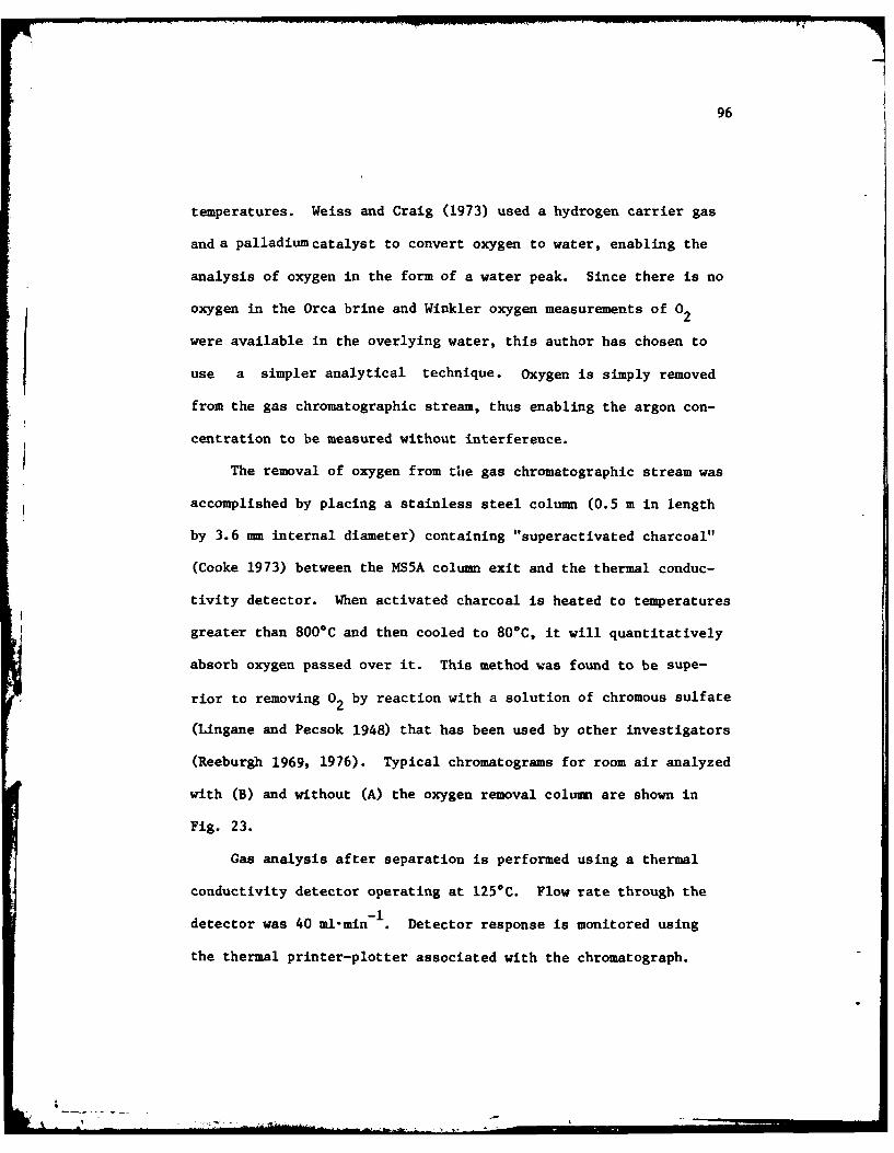
96

temperatures. Weiss and Craig (1973) used a hydrogen carrier gas

and a palladiumcatalyst to convert oxygen to water, enabling the

analysis of oxygen in the form of a water peak. Since there is no

oxygen in the Orca brine and Winkler oxygen measurements of 02

were available in the overlying water, this author has chosen to

use a simpler analytical technique. Oxygen is simply removed

from the gas chromatographic stream, thus enabling the argon con-

centration to be measured without interference.

The removal of oxygen from the gas chromatographic stream was

accomplished by placing a stainless steel column (0.5 m in length

by 3.6 m internal diameter) containing "superactivated charcoal"

(Cooke 1973) between the MS5A column exit and the thermal conduc-

tivity detector. When activated charcoal is heated to temperatures

greater than 800*C and then cooled to 80*C, it will quantitatively

absorb oxygen passed over it. This method was found to be supe-

rior to removing 02 by reaction with a solution of chromous sulfate

(Lingane and Pecsok 1948) that has been used by other investigators

(Reeburgh 1969, 1976). Typical chromatograms for room air analyzed

with (B) and without (A) the oxygen removal column are shown in

Fig. 23.

Gas analysis after separation is performed using a thermal

conductivity detector operating at 125*C. Flow rate through the

detector was 40 ml-min - I. Detector response is monitored using

the thermal printer-plotter associated with the chromatograph.

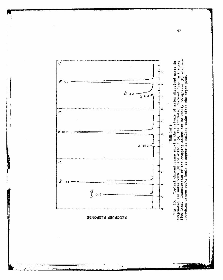
97

00

LI 0) '0

0 k. 0 0

V- f = N~

0~ z Vm o61 z C%4

44M -4 1

" Co-H 4 A I 'd,

U'i 0)

a Q 0 41

t:I m 00

44

0* p 0

0 4-4 -4___ __ __ ___ __ __ ___ __ __ __ 0 a to

. 0OH 0

0 u0 0

3SNdS4 w (U O33

98

Peak areas are automatically integrated and retention times recorded

by the microprocessor system of the 5830A gas chromatograph and

are automatically reported along with the peak area percentages.

A typical chromatogram for Orca Basin brine is shown in Fig. 24.

The chromatographic system was standardized for argon and

nitrogen analysis by injecting standard volumes of dry air into

the column using a calibrated sampling loop (0.493 ml) and an auto-

mated sampling valve (SSV). The gas concentration in the sample

in units of ml (STP)/ml is given by

A V T PC =_2s . __ . __R . - . C (14)x As V T S P Cs

where Ax and As are the peak area for the particular gas in the un-

known sample and the calibration mixture, respectively; C is the5

standard gas concentration (v/v); V is the sample loop volume andg

V is the liquid volume. P and T are the pressure and absolute

temperature in the sample loop; and P and T are the standard0 0

conditions of temperature (273.150 k) and pressure (I atm) for

gases. Corrections for nonideality are not necessary for argon,

nitrogen or methane under these conditions (see Table 1).

The glass container water samples taken from the Nansen

bottles were analyzed using the same chromatographic system used

from the piggyback (PB) samples. The gas stripping system de-

scribed above was also used, but it was modified slightly to

account for the varying requirements of the glass samplers. The

1- H

0.0H r

C-D

z44 ,

U k ,

toJ V4

0

'4 Hd.Culu

41- *

SN1039 ONIddIS - -

UOI1L'llU~lle t'9 - IUVILS - 4: '

Vp4

3SNOdS3-8 83(180038

100

samplers (shown in Fig. 21) were attached to the gas stream be-

tween the PB sample valve (PSV) and the gas stripper (GS). The gas

bypass valve (BVl) was turned clockwise passing clean helium to the

TCD while the sampler gas lines were being purged. In purging the

lines, the water sampler stopcocks are turned so the carrier gas

passes around the sample, through the stripper and drying column

and exits the vent port of bypass valve BVl (see Fig. 22). After

five minutes of purging, the lines are free of any contaminating

atmospheric gases and valve BV1 is returned to its normal position

(counter-clockwise). The carrier gas now flows again to the C

column and detector. After the detector baseline was restabilized

from flow switching, the two three-way stopcocks of the glass

samplers were turned to allow the helium carrier to push the brine

into the stripper for analysis as described above.

Results

Solubility Comparisons

The solubility measurements made on the brine and correspond-

ing sea water samples are given in Table 9. Only a few measure-

ments were made, since the purpose here was not to establish a

complete data set of brine solubility data. A high precision

solubility data set would require microgasometric equipment (Doug-

las 1964) which was not available. The object of these measure-

ments was simply to determine whether , not the equations defined

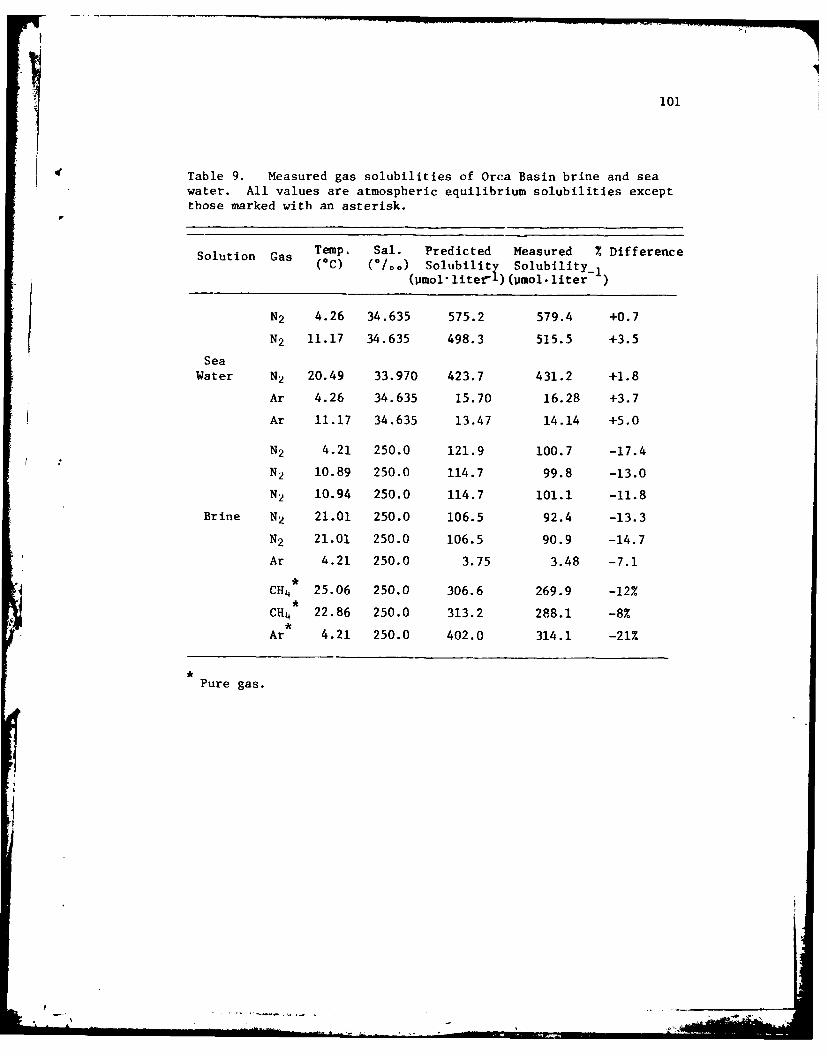
101

4 Table 9. Measured gas solubilities of Orca Basin brine and seawater. All values are atmospheric equilibrium solubilities exceptthose marked with an asterisk.

Solution Gas Temp. Sal. Predicted Measured % Difference(°C00o Solubilty Solubility _,( mol" litef 1 ) (pmol -liter-

N2 4.26 34.635 575.2 579.4 +0.7

N 2 11.17 34.635 498.3 515.5 +3.5

Sea

Water N Z 20.49 33.970 423.7 431.2 +1.8

Ar 4.26 34.635 15.70 16.28 +3.7

Ar 11.17 34.635 13.47 14.14 +5.0

N 2 4.21 250.0 121.9 100.7 -17.4

N 2 10.89 250.0 114.7 99.8 -13.0

N 2 10.94 250.0 114.7 101.1 -11.8

Brine N 2 21.01 250.0 106.5 92.4 -13.3

N2 21.01 250.0 106.5 90.9 -14.7

Ar 4.21 250.0 3.75 3.48 -7.1

CH4 25.06 250.0 306.6 269.9 -12%

CH4 22.86 250.0 313.2 288.1 -8%

Ar 4.21 250.0 402.0 314.1 -21%

Pure gas.

Ii

102

by Weiss (1970) could be extrapolated from sea water salinities

to the higher salinity of the brine. This extrapolation was be-

lieved to be feasible since the major factor governing gas solu-

bility in saline solution is the temperature. Salinity has a

smaller effect. Yet, since the constants for salinity in Eq. 5

are small relative to the temperature coefficients, they can cause

a large error to be propagated in any extrapolation process. The

measured solubility data from this work is compared with the pre-

dicted solubility values in Table 9. Percentage differences be-

tween measured and calculated values are indicated.

Due to low solubility of argon in brine, it was difficult to

measure precisely the argon concentration which resulted from

equilibrating the brine with air in the equilibration chamber.

One successful argon measurement of the atmospheric equilibrium

solubility of argon was made at 4.21°C. At higher temperatures,

however, the digital integrator would not sense the small argon

peaks with enough regularity to integrate them accurately. Thus,

pure argon was used to measure the Bunsen coefficient of argon.

Also, the concentration of methane in the standard atmosphere (1.41 ppm;

Prabhakara et al. 1974) does introduce enough methane into the

equilibrated brine to measure with a thermal conductivity detector.

Pure methane was used to determine the Bunsen coefficient of that gas

as well.

The solubility data for the brine for all three gases

103

indicated that the equation of Weiss (1970) predicts a gas concen-

tration in the brine that is over ten percent higher than the

measured values. This agreement is not bad, considering the diffi-

culties in extrapolating the equation to salinities an order of mag-

nitude higher than was intended. Also, the Orca brine is not just

a higher concentration of sea water. It is a sodium chloride

saturated solution, with a mixture of other components. For

example, total carbon dioxide of the brine is twice normal sea

water values (Sackett et al. 1979). These other compounds also

contribute to the fact that lower values were observed than were

predicted.

The equilibrated normal sea water samples analyzed by this

procedure show a slight supersaturation, in the range of one to

five percent. This supersaturation was expected as has been dis-

cussed previously. These results indicate that it was not a com-

plication of the analytical technique which caused the lower levels

of argon, nitrogen, and methane solubility, relative to the calcu-

lated values. The true values are probably lower than predicted

ones, due to the differences in salt content between sea water and

the brine, and due to difficulties in extrapolating empirical

equations beyond their working range. This information

implies that either the equation does not follow the chemistry at

the higher salt concentrations or that the nature of the inter-

actions change under hypersaline conditions. From data on the

104

changes in ionic activity as a function of increased ionic strength

(Harned and Owen 1950), there is some indication that the latter

is the case. However, that problem is not germane to this dis-

cussion.

The solubilities of argon, nitrogen, and methane are low in the

brine, yet the measured values are relatively close to the

predicted values. These low solubilities and the gas levels in the

brine explain the effervescence which occurs when the brine is

brought to the surface. Effervescing gas bubbles were captured on

four samples taken directly from Nansen bottles on cruise EN-32 of

the R/V Endeavor. One ml of this gas was analyzed by direct in-

jection into the gas chromatograph. The gas collected was found

to contain 1.1% argon, 63.7% nitrogen, 34.6% methane and 0.6% car-

bon dioxide (average of four samples). Although the methane levels

are higher in the brine than nitrogen (see next Chapter), there is

more nitrogen in the effervescing gas, since nitrogen is less sol-

uble in the brine than is methane (Table 9).

Dissolved Oxygen

Dissolved oxygen has been measured on every Texas A&M cruise

to the Orca Basin. The original data of McKee and Sidner (1976)

and the plot of Shokes et al. (1977) were presented in Chapter I.

I shall not give all of the newer data. The data from four

cruises (77-G-2, 77-G-13-I, 77-G-13-III, and 78-G-2) are presented

k_____

105

in Fig. 25. These four oxygen and sigma-t profiles were taken

over the span of one year. The oxygen profiles from each cruise

show oxygen values at the top of the basin (2000 m) which are

fairly typical of deep Gulf oxygen concentrations in this area,

approximately 225 Umol. liter- . As density begins to increase

(along with salinity) from the deep Gulf levels, oxygen concentra-

tions begin to decrease gradually from about 200 umol'liter- I at a

depth of 2175 m, to near zero but not exactly zero at about 2215 m.

This same pattern can be seen in all the profiles. Below this

gradual oxygen gradient there is a region of approximately 20 to 30

m where the oxygen concentration is very low, but measureable. The

oxygen levels are between 2 and 10 Umol-liter- I in this nar-

row zone, and absent or less than the Winkler detection limit below.

The anomalously low dissolved oxygen values are paralleled by

a change in the slope of the temperature profile (see Fig. 10).

The change in temperature is not as obvious as the oxygen change

(step) when viewed from temperature data taken only from deep-sea

reversing thermometers. However, examination of the trace taken

from the STD (Fig. 10) clearly shows the discontinuity in temper-

ature that is associated with this step in the oxygen profile.

The temperature gradient in this region is different from the

gradient either above or below. This oxygen step-like feature is

in the region where the salinity is increasing from 50 to 70o/..

(Fig. 11). The feature is a persistent one and is not an artifact

106

b

DISSOLVED OXYGEN (pmolliter-)

0 80 160 240 0 80 160 240

2000 o

77-G-2 77-G-13-I

2100 - 1 , ,',P

FA

2 2 0 0 -.--- ---------------------- 0

20

00

U.,

E 2300

- 2000

c 77-G-13-M 78-G-2

2100 -

2200 ----------- ------00

2300 I, I i26 28 30 32 34 36 38 40 26 28 30 32 34 36 38 40

SIGMA-tFig. 25. Dissolved oxygen profiles measured by the micro-

Winkler technique (Carpenter 1965) for four different Texas A&Mcruises during 1977 and 1978. Note the persistent step in theoxygen profiles. There appears to be a systematic error in the77-G-2 oxygen data. However, the shape of this profile is con-sistent with the other cruises.

9

107

of the Winkler dissolved oxygen technique.

Argon and Nitrogen

Attempts to sample and analyze the Orca Basin brine for argon

and nitrogen were made on four cruises during 1977 and 1978. The

early efforts yielded only limited success. Plastic syringes used

on the first cruise allowed gas to diffuse out of the sample before

analysis. The sampling systems described in the previous section

were used on the last three cruises (77-G-13, 78-G-2 and EN-32).

Even using these more sophisticated techniques, some samples were

contaminated with atmospheric gases or depleted due to degassing of

the brine. Criteria for determining the reliability of the data

were established. One evaluative method was examining the methane

concentration of each sample. Since methane is relatively constant

I in the brine (Sackett et al. 1979), extremely low methane concentra-tions in the brine samples would indicate gas loss before sample

analysis. Nitrogen/argon ratios were also used in sample evalua-

tion. Samples which had both an unusually high nitrogen/argon

ratio high argon concentrations and very low methane levels were

obviously contaminated with air (N 2/A in air = 83.6) and these data

were discarded.

In the highest salinity brine (S = 262*/..), 25 measurements

of nitrogen were reliable and 9 argon values were believed correct.

The number of argon values is lower since this gas is found in very

low concentrations in the brine and the gas chromatographic

108

peaks for this gas were not always integrated properly. Also, the

standard for this gas was air and could only be determined when

the activated charcoal column was in place in the analysis system

(AC, Fig. 22). Since the column was not always used in the analy-

sis system, fewer total determinations of the argon were made in

the brine.

Nitrogen values from the brine averaged 568 Umol.liter- I (a(

70) while the argon measurements averaged 15.6 pmol.liter-l ( = 1.2).

Measured atmospheric solubilities of these gases in the brine at

4.21C (Table 9) were 100.7 pmol'liter- I for nitrogen and 3.5 pmol"

liter- for argon. These values represent a supersaturation in the

brine of 560% and 450% for nitrogen and argon, respectively. The

reliable measurements of argon and nitrogen are plotted in Fig. 26.

Data in this figure are a composite of gas data taken with the

pressurized piggyback samplers (open symbols) and Nansen samples

collected in glass containers (closed symbols). Methane data

analyzed at the same time (discussed in the next chapter) are pre-

sented in Fig. 26 as a reliability comparison and to indicate the

demarkation line between Gulf water (no CH4 ) and the brine (aver-

age CH4 = 714 Umol'liter- ).

One nitrogen point is not plotted, although it could be signif-

icant to the following discussion. The nitrogen gas concentration

at 2234 meters on cruise 77-G-13 was measured at 1061 pmol-liter-1

using a piggyback sampler. The argon concentration was 9.86 pmol.

A'

109

J=

METHANE & NITROGEN (Wmol- liter')

6 260 460 660 8002100 ,' 1 1 1

0cH4 ..

o Brine Saturation

~CH 4 0'2200 N22200- ORCA BASIN

__ UII

a2300 . 0

o 0 Nansen tottles o I

0 P-ggyback battles : •r o0 0 ,l000

2400-

10 20ARGON (iJmol liter-,)

Fig. 26. Vertical profiles of dissolved argon, nitrogen,

and methane through the Orca Basin interface region into the

high salinity brine. The N2 /Ar ratio in the brine is 36.4.

iii

110

liter and the salinity of the water at this depth was 64.65o..

This sample is found in the oxygen step region where 02 levels

ranged from 4-20 pmol-liter- (Fig. 18). Several other nitrogen

measurements just above the high salinity brine also reflect levels

higher than would be predicted from atmospheric equilibrium solu-

bility. The bulge in the N2 distribution between 2185 m and 2250 m

(Fig. 26) also shows supersaturation, while the value at 2169 m

(N2 = 567 Pmol-liter - ) is within 1.5% of the predicted sea water

solubility value. The one very high nitrogen value in the oxygen

step region may be questionable, since the associated Ar measurement

is so low. The N2 /Ar ratio (108) cannot, however, be accounted for

by atmospheric contamination. The other N2 and Ar data in this

region are considered reliable for the following discussion.

Discussion

Dissolved Oxygen

The dissolved oxygen profiles in the Orca Basin (Fig. 25) show

a general decrease through salinity transition zones TI and T2. A

constant but low oxygen level was observed in transition zone T3.

Oxygen was absent in the interface region and high salinity brine.

Oxygen is the first oxidizing agent consumed in the organic matter

decomposition process (Richards 1965). The equation used to

describe oxygen consumption is

111

(CH2 0)1 06 (NH3 )1 6 (H3 PO4 ) + 138 02- 106CO2 + 16HNO3 (15)

+ H PO + 122 H03 4 2

In this decomposition reaction, 138 umol of oxygen are consumed for

every 106 imol of carbon dioxide that are produced. If the brine

was originally Gulf sea water (T = 4.2, S = 35O.o.), it would have

had an original oxygen concentration of 322 umol. liter- 1 (Weiss

1970). Removal of this amount of oxygen via Eq. 14 would produce

247 pmol of carbon dioxide. The amount of carbon dioxide that has

been added to the Orca brine due to decomposition has been calcu-

-1lated as 2290 mol'liter (Sackett et al. 1979). Thus, the CO2

input from oxygen consumption would account for only 11% of the

total CO2 input. The major input of carbon dioxide must result

from other, anaerobic decomposition processes which will be dis-

cussed in the next chapter.

The decrease in oxygen in the transition zone must be due to

oxygen consumption as described in Eq. 14. The convex downward

slope of the profiles in regions Tl and T2 are indicative of

consumption in that region. The increase in excess total carbon

dioxide through this region is about 470 Umol'liter-1 (Sackett et

al. 1977), while oxygen decreases from 225 to 10 Umol'liter- 1 .

This oxygen decrease via Eq. 14 would result in the production of

165 Umol-liter- 1 of carbon dioxide. That value represents 35% of

the amount supposedly produced in this region. If oxygen is

I

112

consumed in producing this carbon dioxidt, one can assume that 65%

of the excess CO2 in this region comes from anaerobic decomposition

or from diffusion of CO2 from the zone below.

The oxygen step zo,, has a low but measurablh amount of oxygen.

Water in this zone has a characteristic salinity between 3U and

70o/o. All samples in this salinity range have measurable oxygen

less than 15 pmol'liter- . No exceptions have been found. The

microWinkler oxygen technique (Carpenter 1965) is not very precise

in this area due to interferences at low concentrations. However,

even with care to eliminate the possible effect of nitrite on the

samples (Broenkow and Cline 1969), oxygen showed some variability

in the step region, i.e., transition region T3. Although it is

impossible to be certain, the oxygen levels in this region seem to

be relatively constant. They decrease to zero within a very small

depth region where salinity increases above 700Ioo, i.e., in the

interface region.

This step-like feature in the oxygen profile is an unusual

occurrence. Like other variables in the ocean, this feature must

represent a balance between transport processes and removal mech-

anisms. Oxygen can be transported into this region by diffusive

mixing from above, and by possible advection of new water/brine

from the side. The change of oxygen with salinity in this zone

(Table 7) is much lower than in either of the regions above. This

may result from the low oxygen concentration, if the rate of

113

consumption is first order with respect to concentration. However,

this is improbable. In other environments with low oxygen values,

oxygen profiles decrease smoothly to zero without going through a

step (see, for example, Richards 1975).

Nor does this step-like feature appear to be the result of

input of new brine into the basin. The density of the high salin-

ity brine is greater than the density of the water in the step

region and would not remain on top of the interface as this feature

does. A biological mechanism may explain the oxygen levels found

there. In this region, the salinity increases from 50 to 70%.

Just above this region (based on oxygen data), LaRock et al. (1979)

observed a large increase in ATP and uridine uptake, with lower

values below. It is possible that the microbial population which

mediates consumption of oxygen in the ocean is inhibited by sa-

linities greater than 50*o/o. If the microbes cannot metabolize

oxygen effectively, the oxygen input due to diffusive mixing from

above (see Chapter II) would be very slowly consumed and might

remain in balance with oxygen consumption causing the observed

feature.

Inhibition of bacterial activity in hypersaline waters exists

in the Red Sea brines. However, most of this work has been done

on the anaerobic bacteria. Tr~per (1969) found that bacterial

sulfate reduction is inhibited at high salinities, with signifi-

cant decreases in microbial activity at 60*o/. and greater. The

%.~4 t..........

114

Orca Basin brine is not sterile (LaRock et al. 1979) like the hot

metalliferous Red Sea brine (Watson and Waterbury 1969). A slowing

of bacteria], activity, however, combined with slow or periodic

oxygen mixed into this region could produce the feature that was

observed.

Argon and Nitrogen

The argon and nitrogen distributions in the Urca B~asin can be

divided into two zones of interest: the transition zone and the

high salinity brine. In both of these zones, nitrogen gas concen-

trations are higher than would be predicted on the basis of solu-

bilities. The nitrogen data in the high salinity brine show some

random variability, with a relative standard deviation (RSD) of 12%.

However, within the precision of the sampling and analytical tech-

niques both nitrogen and argon levels (RSD = 8%) are considered

constant in the high salinity brine (Fig. 26). On the other hand,

there is an obvious trend in the nitrogen distribution in the

transition zone.

Transition Zone. Nitrogen values were higher in the transi-

tion zone than in either the brine, or the freely circulating

Gulf water above. This increase in the nitrogen levels was found

in the area where nitrate is being reduc Ied to essentially zero. While

the nitrate may not be the main source of excess nitrogen in the

transition zone, denitrification processes must be the cause of

115

the excess nitrogen. The added nitrogen is calculated to be 140

pmolliter- 1, which represents a supersaturation of 25%.

Denitrification is the biological reduction of nitrate or ni-

trite to nitrous oxide or free nitrogen. Denitrification can be

carried on by a wide variety of faculative anaerobic bacteria

(Brisou and Vargues 1961). The source for hydrogen in the reaction

may come from either organic or inorganic substrates (e.g., H2 '

RH2S). Several feasible reactions at 250C are given by Vaccaro

(1965).

2NO5 + 2H + - N 20 + 202 + H20 (16)

AG0 = + 21 kcal.

4NO0 + 3CH - 2N2 + 3CO 2 + 6H20 (17)

AG0 = -475 kcal.

8NO+C6H206 - 4N + 4CO 2 + 2CO + 6H20 (18)2N C612O6 2 3 2 2

AG' = -728 kcal.

When an organic substrate supplies the hydrogen, the reactions are

energetically feasible in aerobic waters. If the hydrogen comes

from an inorganic source (Eq. 16), reaction is feasible only in

the absence of oxygen.

The nitrate levels in the deep Gulf average 23 Umol'liter-1 .

Reduction of 23 Umol of nitrate would produce only 11.5 umol of

116

molecular nitrogen. Thus nitrate reduction alone cannot account

-1for the nitrogen increase of 140 pmol-liter that was observed in

the transition zone. Another source of nitrogen substrate is

needed to provide the starting material for nitrogen gas production.

Two possible sources are ammonia produced from organic material

decomposition at the brine interface or ammonia diffusing up from

the brine. Ammonia levels in the brine (see Chapter IV) are about

500 Pmol-liter-, but diffusion from the brine would be very small.

Possible mechanisms of nitrogen gas formation are shown in Fig. 27.

Ammonia diffusing out of the brine or produced in the oxygen

step region could be oxidized to nitrate and/or nitrite. These

nutrients could be subsequently converted to nitrogen in this low

oxygen environment. The biological oxidation of ammonia to nitrite

then nitrate in sea water has been described in the clas-ic laboratory

experiments of von Brand and his co-workers (cited in Vaccaro 1965).

The oxidation process is mediated by various nitrifying bacteria

including Nitrosomonas and Nitrobacter (Zobell 1946) and Nitro-

socystis (Murray and Watson 1963). These processes are well

documented in the literature.

There is no evidence, however, for the direct conversion of

ammonia to molecular nitrogen. While ammonia oxidation during

denitrification is thermodynamically possible (Cline and Richards

1972), there is little, if any, experimental evidence for the

direct biological oxidation of ammonia to free nitrogen. In the

low oxygen waters of the eastern tropical Pacific, Goering (1968)

detected no oxidation of ammonia during studies of natural

J-

117

N2

NO 3

NO3 +N0 3 NO2

NITROGEM CYCLE

Fig. 27. A schematic representation of the possible pathwaysthrough which organic nitrogen or ammonia may be converted tomolecular nitrogen. All of these pathways are thermodynamicallypossible, but not all under the same conditions.

118

microbial populations. Cline and Richards (1972) also reported no

apparent oxidation of ammonia in their study of nitrate reduction in

the same region. The low ammonia concentrations observed in the

Pacific were attributed to removal of ammonia during bacterial

assimilation, not nitrification to molecular N 2.

For production of molecular nitrogen from ammonia, a two-step

process must exist:

1 2NH4 --- + (NO2 or NO 3) N2 (19)

Oxygen concentration in the oxygen-step region of the Orca Basin

(zone T3) averages 10 pmol.liter-1. Carlucci and McNally (1969) have

demonstrated that oxidation of ammonia to nitrite can occur under

conditions of low oxygen tension, down to 2 pmol.liter- . Such

conditions prevail in the Orca Basin interface region. In the eastern

tropical Pacific, Cline and Richatis (1972) observed the simul-

taneous occurrence of nitrite, along with the apparent loss of

nitrate and suggested that nitrite is an intermediate in the reduc-

tion of nitrate to free nitrogen. Since nitrite does not accumulate

in the Orca Basin from ammonia oxidation, it appears that the

reduction of nitrate to nitrite and of nitrite to free nitrogen

occur simultaneously (i.e., as coupled reactions (Eq. 19) which may

be carried on by the same or different organisms).

Nitrate or nitrite may be the major intermediate in the pro-

duction of nitrogen. Wiesenburg et al. (1977) noted the presence

of high nitrite concentrations (up to 15 pmol.liter- ) in the

1!

119

interface region (transition zone) of the Orca Basin. Their data

(Fig. 28) indicated that the nitrite maximum was found well above

the region of lowest oxygen values. The nitrite maximum may have

resulted from nitrate reduction. A nitrite maximum above the

brine was not observed on subsequent cruises, however. This max-r imum may have been a transient feature, with the nitrite being

subsequently converted to molecular nitrogen as in Eq. 18.

A continuing supply of dissolved oxygen could be provided by

mixing from above. This oxygen could be used in the oxidation

of ammonia. The nitrate or nitrite so produced would in turn be

reduced to N 2as in Eqs. 16-18. These conclusions are valid for

the Orca Basin brine-sea water interface. They are also the same

conclusion Barnes et al. (1975) suggested for the Santa Barbara

Basin sediments. Barnes et al. (1975) examined nitrification and

denitrification in suboxic sediments of the Santa Barbara Basin.

Increases in both dissolved molecular nitrogen and the N 2/Ar

ratio were observed in the sediment pore waters. Nitrogen in-

creases (up to 17% above bottom water values) could not be

accounted for by nitrite (or nitrate) reduction alone. It was

concluded that ammonia, derived from organic matter containing

nitrogen, was converted to molecular N2 through a nitrite inter-

mediate under conditions of low oxygen tension. Since methane is

also present in the sediments of this basin (Emery and Hogan 1958),

the sediment-sea water interface geochemistry in the Santa Barbara

1i20

0

> mN

> I QN

:3- 0'~

V _-I Aj

E.~ E

LLI~~- < :cnc(NJ *

o~ a

C 1-4 r-

I' to.. -4C - C)CO~~~~ I i )4-C) .

W~ .'a

-H $40I(0 CL() O

Z ) c0(

IP 0

I 0 en

I" .-1410C

IS,)IO U *.- u C)

121

Basin may be similar to the brine-sea water interface geochemistry

in the Orca Basin. In both areas, ammonia is being converted to

molecular nitrogen via a nitrate or nitrite intermediate.

High Salinity Brine. Both argon and nitrogen are supersat-

urated in the high salinity Orca brine. The excess gas, relative

to atmospheric solubilities (Table 9), must arrive with the entry

brine into the basin, or be produced in the brine after deposition.

Argon has no known biological source. Production of argon by

radioactive decay of 40K, however, does occur. Craig (1969)

attributed the 10% excess argon in the Discovery Brine of the Red

Sea (relative to the Atlantis II brine) to excess radiogenic 40Ar.

This concept is consistent with a model of the Discovery Brine as

a stagnant overflow from the Atlantis Deep, as discussed by Weiss

40(1969). In the Orca Basin brine, however, radiogenic Ar is

probably not an important constituent of the total argon observed.

It can be calculated (Table 10) that radiogenic argon production

would only be 9 x 10- 7 vmolkg-I during the 7900 year age of the

brine in the Orca Basin. Even if the excess argon came from the

Jurassic LouAnn salt (an unlikely case) an increase of only 2

Umol-kg- would be predicted. The observed excess argon is over

10 Vmol'kg - (Fig. 26). Unlike the Red Sea brines, argon produc-

tion is not important in the Orca Basin.

Molecular nitrogen in the Orca Basin remains relatively con-

stant, below the zone where oxygen is present. There is abundant

122

Table 10. Calculated theoretical production of dissolved argonin the high salinity Orca Basin brine.

Assume the brine potassium content has been constant over timeat the present concentration (0.63 g.kg -1) and that A is pro-duced by radioactive decay of 40K.

K content of brine:

= 0.63gK = kg- = 16.1 mmol.K = kg brine

= 9.7 x 1021 atoms K.kg- I brine

Atoms 40K: (Atomic abundance = 0.0118%)

1.1 x 1018 atoms K. -g 1 brine

Atoms 4 0K decaying to Ar: (Branching ratio = 0.11)

= 1.3 x 1014 atoms.kg- 1 brine

Growth of Ar: (t = 7900y, decay const = A 5.4 x 10- 10 yI

Ar -4 0K (1-e- t) = 5.4 x 1011 atoms Ar.kg - brine

= 9.0 x 10 . 7 mol Ar.kg brine

- . . . .

123

ammonia in the high salinity brine (see next Chapter), but there

is no apparent nitrogen gas production in this zone. Even though

N2 is the thermodynamically stable species in sulfate reducing

environments, a biochemical pathway for the direct conversion of

ammonia to dissolved molecular nitrogen must not exist. Barnes

et al. (1975) also came to this conclusion for the anoxic zone of

the Santa Barbara Basin sediments. They observed near-uniform N2

distribution in the anoxic zone and noted that N2 production would

increase the N2/Ar ratio. In the Orca Basin, the N2/Ar ratio

in the brine was 36.4 (average of 25 points) while the predicted

solubility values for N2 and Ar at 250o/. salinity and 5.650C

gave a N 2/A ratio of 36.5. There was no N2/Ar increase.

Neither nitrogen or argon is being produced in the high

salinity bottom water of the Orca Basin, yet elevated concentra-

tions (relative to solubility) of both gases are observed. One

can show that the observed nitrogen was present when the brine

formed. The sea water which dissolved the salt exposure to form

the brine must be deep Gulf water like that at the basin sill

(T = 4.20C, S = 35*/oo). This deep Gulf water probably originates

from the Upper North Atlantic Deep Water (UNADW), with a very

small component of Mediterranean Sea water (J. Cochrane, personal

communication). Assuming (the extreme) that the UNADW (20C) is

the initial component in the mixture which produces the Orca Basin

sill water, it would have to be mixed equally with water at 6.40C

124

(and 350/ce salinity) to reach the values observed. Since mixing

two waters of different temperatures can cause an apparent super-

saturation (Fig. 19), this mixing effect was investigated as a

possible cause of the supersaturation of N2 and Ar. Such a mixture,

however, would only cause a supersaturation anomaly of 0.1% for

Ar and 0.2% for N2, far below the observed excesses. Having dis-

counted all other possibilities, we are able to conclude

that the Orca Basin brine is simply salt-saturated,deep-Gulf sea

water with the N2 and Ar gases intact. This conclusion is sub-

stantiated by the following discussion.

Argon concentration is plotted against nitrogen concentration

in Fig. 29. All concentrations in the plot are expressed as pmol

per 1000 g H 0 , and are thus not affected by the dissolving or2'

precipitation of salt. The observed concentrations for the Orca

Basin were converted to these units by converting from Umol-liter-1

to pmol-kg- using the density equations of Millero et al. (1979),

and to pmol per 10OOg water using the value of 741.9 grams of H2 0

per kg of brine. The Red Sea brine data, given for comparison,

are from Weiss (1969).

Solubility values for fresh water and 35*/.o sea water (Orca

Basin sill water, OBSW), in equilibrium with air at one atmosphere

total pressure (including vapor pressure) are also plotted in

Fig. 29. These curves (in units of umol'kg - ) were calculated

using Eq. 5 and the coefficients given by Weiss (1970), and were

A ._________________ . ~

125

20ORCA BASIN BRINE

0.C toOC

Fresh Water15 - Sea Water Solubility

o Solubility 10 20

04 (Salinity 35 o/oo)

DISCOVERY20 30 BRINE ,/

000 10 30 40 e //1s''= /

ATLANTIS II/40 BRINE /w /

Orca Basin // ..'Extrapolated ,,

-/0.c //4 /

20 /140/

/

/I0 / . .I I 1.0 250 500 750 1000

N2 )moles/1000 g H2 0Fig. 29. Argon versus nitrogen In the Orca Basin

brine and solubility values for fresh water, 35%/,°sea water and Orca Basin brine in equilibrium withthe atmosphere. Data for argon and nitrogen (Weiss1969) from the Red Sea brines are given for compar-ison.

126

corrected using a value of 965.0 g water per 1000 grams of sea

water. Using Eq. 5, N 2and Ar solubilities were extrapolated to

the salinity of the Orca Basin brine. As was previously discussed,

these extrapolated values are a few percent higher than the ob-

served atmospheric solubilities in the brine (Table 7), but are

close enough for the comparisons presented here. The Ar/N2 ratio

in air is also plotted in Fig. 29.

Fig. 29 indicates that the observed N and Ar concentrations2

in the Orca Basin are supersaturated approximately 250% with

respect to brine in equilibrium with air at 5.60C. Although this

difference could be produced by addition of radiogenic argon and

large amounts of air, the existence of such a natural process is

extremely improbable. Contamination can also be excluded. Bulk

sample loss would move the brine N 2 /Ar value in Fig. 29 along a

straight line toward the origin, while air addition would move the

point away from the origin along a line with a slope equal to the

Ar/N 2ratio in air. Neither case is observed here.

The large saturation anomalies in Ar and N 2can be best ex-

plained, not by gas production, but rather by the simple addition

of salt to deep Gulf water - the mechanisms proposed by Shokes

et al. (1972) for Orca brine formation. Comparison data for the

Orca Basin - Gulf water and Red Sea brine - Red Sea water systems

are given in Table 11. Weiss (1969) and Craig (1969) explained

the N 2and Ar saturation anomalies in the Red Sea brine on N 2

127

U)GJ r- or- -*L N 1 C

w Cm r-. r- .1 0'I %Do ego 0 -4 4 (

(d 0):1cfC -4C O vo4

> cdo .)w") W (V " a c

U - 04wcen %D 0)a

44 r- W4- to A I ' I (

4) 0o

o bo ) 41 >

44--0 -H

,-I O ~j.- eUW)-. 4 04 :30

En 4).-4 . 4 :1 >A 0N M% 0 m4 A w m

0c~ Ai 41-

0) 0) cc In4

w~U0 4-4 0)t2L 0d Cf 0)C' '' -H

V V cd0 co ev . . I

01- m 0 > HrI0)L q aL )P40) " d i0U) .U'-4 r. c 0)

) U $4,0).4 W k. C14 0)

00

.- U 0

m) A14 U) u)

w 0) C0 C- 0.w 0 u- 0 t" W $4 --4

0 0 (Au n 0 1

Z) U4 ) C.) U-0,4 >~

W U 0)4 C.J"td Wd) r-4 c 1-1

L. 5

128

production from organic matter in both brines and radiogenic Ar

production for the Discovery Brine only. Considering the above

discussion, these mechanisms are not operative in the Orca Basin

brine. Both average N2 and Ar values are slightly higher than the

predicted values (Table 10), but the uniform differences (13%) in

each indicate a physical rather than a biochemical or radiogenic

effect. This difference may be due to some of the assumptions

(e.g. initial equilibrium) made in calculating the theoretical

values. If error limits for N2 and Ar are taken as twice the

standard deviation of the determinations, then the uncertainty

envelope for the Orca Basin, Ar/N2 point on Fig. 29 encompasses

4.2*C and 35*/oo on the sea water solubility curve. Thus, all

the Ar and N2 in the Orca Basin high salinity brine can be aoount-

ed for by the addition of salt to deep Gulf water.

Shokes et al. (1977) surmised that the brine in the bottom

140 meters of the Orca Basin resulted from the underwater disso-

lution of a surface or near-surface salt deposit on the basin

slope. This exposed diapir must be dissolving due to contact with

deep Gulf water and the resultant brine flows down the slope into

the bottom of the basin. The previous evidence for this mechanism

of formation of the Orca Basin brine has been:

1. The decreasing salinity gradient in the sediments.

2. The relative ion abundances of potassium and calcium

129

relative to sodium, which are unlike the Red Sea

brines and indicate a low temperature halite disso-

lution.

3. The bromine content of the Orca Basin water, which indi-

cates that the brine is formed by the dissolution of an

evaporite deposit rather than by an exaporative process.

4. The seismic data of Addy and Behrens (1980) which indi-

cate that exposed salt diapirs do exist in the vicinity

of the Orca Basin and support the earlier contentions

of Shokes et al. (1977) concerning the location of the

source salt.

The other piece of information which now emphasizes the

origin of the brine is the nitrogen-argon relationships determined

as part of this study. Dissolved argon and nitrogen data provide

independent evidence that the Orca brine did form due to low

temperature dissolution of a salt deposit by sea water. Since the

gas data is not based on the major ions, which have been used in

the other evaluation techniques, the conclusions based on these

data are independent of the ionic balance percentages in the salt

that was dissolved. The only assumption that was made, in using

the gas data to make this evaluation, was that the sea water that

participated in the dissolution of the salt diapir had an original

salinity of 35o/@.. The temperature at which the salt water was

130

saturated with brine is estimated from Fig. 29 to be between 0 and

5°C and further supports the low temperature dissolution assumption

of Shokes et al. (1977).

131

CHAPTER IV

DISSOLVED REDUCED GASES

Organic matter is thermodynamically unstable in sea water and

eventually decomposes into various small molecules in the C-N-S-H 20

system. Decomposition of organic material in anoxic basins and

sediments has been extensively studied (see for example, Richards

1965). These studies are important to an understanding of marine

geochemistry since such environments enable us to determine the

mechanisms by which organic material is recycled from the sediments

back into the water column.

The most widely accepted model of organic matter decomposition

is related to the free energy of the oxidant involved in the dia-

genesis process. Organic matter [assumed to have an idealized

composition of (CH2 0) 10 6 (NH 3)1 6 (H 3PO 4 1 (Fleming 1940; Redfield

1958)] is oxidized by the oxidant having the greatest free energy

yield per mole of organic carbon oxidized (McKinney and Conway

1957; Richards 1965; Claypool and Kaplan 1974). When an oxidant

is depleted, the oxidant with the next highest energy yield is

consumed until every oxidant is removed, or until all organic car-

4 bon has been depleted. Table 12 (Froelich et al. 1979) summarizes

the predicted sequences of reactions. In anoxic marine environ-

ments, the decomposition reactions are mediated by denitrifying,

iron oxide reducing, sulfate reducing and methanogenic bacteria

132

*)

Table 12. Oxidation reactions of sedimentary organic matter.

1. (CH20)lo6(NH3)16(H3PO4) + 138 - -106 CO2 + 16 HNO 3 + H3PO4 + 122 H20

AG*' = -3190 kJ/mole of Glucose

2. (CH20)6(NH3)16(H3PO4) + 236 MnO2 + 472 +-- 236 Mn2+ + 106 CO2

+ 8 N2 + H3PO4 + 366 H20

AG*' = -3090 kJ/mole (BIRNESSITE)

-3050 kJ/mole (NSUTITE)-2920 kJ/mole (PYROLUSITE)

3a. (CH2 0) 1 0 6 (NH3 ) 1 6 (H3 PO4) + 94.4 HNO 3----- + 106 CO2 + 55.2 N2 + H 3PO4

+ 177.2 H20

AG"' = -3030 kJ/mole

3b. (CH2 0) 1 0 6 (NH3 ) 1 6 (H3P0 4) + 84.8 HNO 3-----*. 106 CO2 + 42.4 N2 + 16 NH3

+ H3PO4 + 148.4 H20

AG*' = -2740 kJ/mole

4. (CH2 0) 1 0 6 (NH3 ) 1 6 (H3P0 4) + 212 Fe203 (or 424 FeOOH) + 848 H -

424 Fe2+ + 106 CO2 + 16 NH3 + H 3PO 4 + 530 H 20 (or 742 H2))

AG°' = -1410 kJ/mole (HEMATITE, Fe203)

- 1330 kJ/mole (LIMONITIC GOETHITE, FeOOH)

5. (CH0)I06(NH3)(H4PO ) + 53 SO4 2- 4 106 Co2 +16NH 3 + 53 S2 - + H PO

+ 106 H20

AG*' = -380 kJ/mole

6. (CH20)10 6 (NH3)1 6 (H3PO4 ) - 53 CO2 + 53 CH4 + 16 NH3 + H3 PO4

AG*' = -350 kJ/mole

See Froelich et al. (1979) for an explanation of how free energieswere calculated.

133

(Reactions 3-6), resulting in the production of N2, NH3, HS, CO2P

HCO3, CH4, and other related compounds. Interstitial waters from

the upper meter of anoxic marine sediments often represent the

early stages of the diagenetic process (Thorstenson and MacKenzie

1974; Froelich et al. 1979), while deeper sediments usually exhibit

complete sulfate reduction and large increases in methane and car-

bon dioxide (Hammond 1974).

Anoxic waters overlying reduced sediments have chemical

distributions which reflect the oxic and suboxic processes (Re-

actions 1-4, Table 12) taking place at their oxic-anoxic sea water

boundary, as well as the sulfate-reduction-catalyzed reactions

taking place in the water and sediments. The combined influence

of these decomposition processes in anoxic marine waters has been

described for the various nutrients (Richards 1965; Richards et

al. 1965; Fanning and Pilson 1972). Only a few studies, however,

(Atkinson and Richards 1967; Linnenbom and Swinnerton 1969; Ree-

burgh 1976; Cohen 1978) have considered the role of various re-

duced gases in anoxic waters.

In many anoxic areas (e.g., Cariaco Trench) the stability of

the water column is relatively low (see Table 5), and periodic

inputs of oxygenated water replace some of the anoxic waters. In

these other basins, the oxygenated, renewal water both dilutes

and oxidizes the reduced products (nutrients and gases) of

anaerobic decomposition (see Table 12). In the Orca Basin,

- -----. --- t-

134

however, the great stability of the hypersaline water (-250 /o)

precludes input of any significant amount of renewal water. With

no input of renewal water, and with little (other than diffusive)

loss of decomposition products from the brine, the Orca Basin is

an ideal location for studying the processes on anaerobic

decomposition.

Shokes et al. (1977) have described nutrient distributions

resulting from the anoxic conditions in the basin. Phosphatel-

levels increased from 2.5 umol-liter- I above the brine to between

60 and 80 Umol-liter- I near the bottom, with no obvious trends in

the depth profile within the brine. Silicate likewise increased

from 25 Umol'liter to over 235 imol-liter , while nitrate de-

creased from 23 umol-liter- above the brine to zero level through-

out the brine. This chapter presents a detailed description of

the geochemistry of reduced gases (CH4, C2H6, C3H6, N20, NH3 and

H2S) in the waters of the Orca Basin, and describes the distri-

butions which have resulted from the anoxic, hypersaline conditions.

Methods

Sampling

Observations of reduced gases were made on five cruises

aboard the R/V Gyre during October 1976 (76-G-10, April 1977 (77-

G-2 and 77-G-3), November 1977 (77-G-13), and one aboard the R/V

.€

135

Endeavor in February 1979. Stations were taken in both the north-

ern and southern lobes of the Orca Basin and samples were collected

both above and in the brine between 2000 m and 2500 m. Most water

samples for reduced gas analysis were taken with standard 1.2-liter

teflon-coated Nansen bottles. As was previously discussed, sam-

pling with 5-liter Niskin bottles proved ineffective since gases in

the Orca Basin brine are supersaturated at atmospheric pressure and

degas as hydrostatic pressure is reduced. Since Nansen bottles

have a ball valve-type closing apparatus these bottles seemed to

inhibit degassing and gave representative results for most gas

measurements in the brine.

Sampling from the Nansen bottles was performed initially by

transferring the brine to glass bottles (cruise 76-G-10) for later

analysis of the reduced gases. This technique gave low values,

due to the effervescence which occurred during gravity transfer

of brine from the Nansen bottles. During subsequent cruises, brine

samples were drawn directly from the Nansen bottles into helium

purged glass syringes which were used either to inject samples

directly into an all-glass stripping chamber (Swinnerton et al.

1962) or to equilibrate the water with helium (McAuliffe 1971).

Samples for methane analysis were collected in piggyback samplers

on cruises 77-G-13 and 78-G-2, to compare the Nansen samples with

the pressurized samples. On cruises EN-32, samples for methane

analysis were also collected in the all glass sampling containers

shown in Fig. 21.

136

Analytical Techniques

The data for this chapter on reduced gases in the Orca Basin

brine include measurements of oxygen, nitrous oxide, hydrogen

sulfide, ammonia, methane, ethane, and propane as well as determi-

nations of temperature, salinity, iron, sulfate, nitrate, and

phosphate. A complete set of these values was needed to make a

comprehensive evaluation of anaerobic decomposition processes out-

lined in Table 12, but it was impossible for one researcher to

make all of these measurements simultaneously on every cruise to the

Orca Basin. Table 13 gives a description of the various parameters

measured on each of the six cruises as well as the analyst who was

responsible for providing the data for this comprehensive inter-

pretation. A list of analytical techniques that were used is

given in Table 14.

Briefly, temperature was measured using standard reversing

thermometers attached to Nansen bottles. As previously mentioned,

salinity was obtained by performing either weight or volume di-

lutions (density corrected) to near 35Y/.,. followed by analysis

using a Plessey Environmental Systems 6230N inductive salimometer

which was standardized against standard sea water. Salinities

measured by this method are only relative since the Orca Basin

brine is not just a concentrated sea water with ion ratios equiv-

alent to those of normal sea water.

Dissolved oxygen was measured by a modification (Broenkow and

137

4II-.Q

ww-

11-0

0I

U 44 0

0 4j0Mw

$4 00000 -W 4-

u 0

44

CL 0 0 H- H- H- H- -

$4 0 2

JJ E-4 E-4 H H p

>00 0 E-4 E-4 p. F- 14 1 0

0 w9-4 CC

44~ 0 1-4 w- >- -4 14 I 2

0 41 1- H- E4i P- E-4 4

00 Cdd 04

02 4(4 m K 0

1-4 00 4

U4 4 Cd $4 % l - r bw0 H

m 0

138

C4~ 0

- ~ cy 0% I

-4-% 4

w2 C\ $4 M0: 0 41

04 0 W) 0, M''0)~ ~ '$.4 . I 44 C s C4 W-

0 - 0 1\4 8

1. .I .-4 0 M0 -. 0 C7%. 00- 0 r-f 01 t4 02rI $> E- ) ~. . .~~~n .

010. ~~~- I .. 0-

-H - a

0 0 0It 4. U 44

= -W 4JJ0o 0 o- z- 0 - 0

Ui A1. C 0 0

P. 0 00 41 0 .u

*-H- 0 ; ;001 V $ -H

ca 0 430 4.3 r 4-1 V4H w .$4.3el) 00.0 W'- -H 4J 14C 4. 0

140 0 k 43 0 4 0 *H 4J0 C)' 00q 41 w o. 0 4.1 H 4 00 a) 0)c: c

1-i 02 $44 024.3 0 s p) r-40 004 00 M 4J 0 w 4 1.4 a0 w4-

44 w2 14 0 0 0 w1 CJ 0 1 0 10 oC) w u C) u 413 .- I 0 -4 4 c: -H 0 )0

V0 w -H r-I 0 cc Ow0. 0 0. 4-0 0 > 14M 0 . u C0 0. 002 4.3 P4 -0 r H 0 4.300 ) v 00 -H 00 0

01 d 4-1 H V1 -H V4 Ho 00 pr. 04C) 1 413 -41.4 -H 413 -40

-H 0 VE 0 0 0 0 0 0. 0.0W>H k - 0 $.. 41J N a 00 u .0.m2 u) C) P 01.. 0 ' 0 1 10 0 0c.

01.4 *H ).=0 ) *H ..00, 1.4p 0 $4.a

0

4-40

4.3 00 -H

f -4 0NM VqC0

4) 401 0 4.

a 01 0' 0 0 V-i C:.4c

0 -4 0 41 4 4 -H " C)

.0 U 0 $4 -C V4 140 -H4 -HO w0d cnwN z

. ......... .. . . . . . . .

...... . ...... ..... . . ...

139

Cline 1969) of the microWinkier method of Carpenter (1965) as was

described in the previous chapter. Nutrients were measured coloro-

metrically by AutoAnalyzer using dilutions to bring the concen-

tration of salts down to a level where they did not inhibit the

relative responses to the nutrients alone. Dilution was also

necessary due to the high nutrient concentrations observed. Inor-

ganic phosphate was determined by the ascorbic acid-potassium anti-

monyl tartrate method of Murphy and Riley (1962) as modified for

use on the AutoAnalyzer by Atlas et al. (1971). Nitrate ions

were determined by the cadmium reduction method of Armstrong et al.

(1967).

Ammonia was measured by three different techniques. On cruise

77-G-2, ammonia was measured using an Orion Research Model 95-10

specific ion electrode standardized against NH4Cl-ammonia solu-

tions. This probe had been used previously for studies of inter-

stitial waters and had proven to be very effective for samples

of high concentration. There seemed to be very little, if any,

salt effect associated with this probe at the high NH3 levels

found in the Orca brine. On cruise 77-G-3, ammonia was determined

manually using the phenol hypochlorite method of Solorzano (1969).

Samples for ammonia were taken in syringes or pipettes filled di-

rectly from the Nansen bottles and introduced into 50 ml serum

vials below the surface of the complexing reagents. Ammonia

samples collected in this way seem to be little affected by the

140

degassing which caused inaccuracies with other reduced gas measure-

ments. On cruise 77-G-13, ammonia was determined by AutoAnalyzer

using the phenate method of Weatherburn (1967) modified for use on

the AutoAnalyzer II. Samples for AutoAnalyzer analysis were

transferred into sample cups before analysis. There was a pos-

sibility of degassing in these samples since they remain open to

the air while they await analysis. However, no apparent loss of

ammonia was observed after sample collection, as evidenced by the

consistency of the three methods.

Hydrogen sulfide was determined using the mixed diamine

reagent method of Cline (1969). Samples were drawn from Nansen

bottles directly into pipettes and the brine sample was introduced

into the acidified reagent under the liquid surface, thus avoiding

any contact with air which would rapidly oxidize free sulfide.

Sulfate was measured gravimetrically using a standard barium pre-

cipitate method described by Vogel (1968). Dissolved iron in the

water column was also measured using the ferrozine method of

Stookey (1970).

Nitrous oxide was determined on cruise 77-G-13 by a technique

similar to the one described by Cohen (1978) with modifications:

an Ascarite column was placed after the magnesium perchlorate

column to remove CO2. An electron capture ( 63Ni) detector oper-

ated at 300*C, was used in conjunction with a Hewlett-Packard

5830A gas chromatograph for sample analysis, after separation on

141

a Porpak Q column. Calibration was accomplished by comparing the

measured values against a standard calibration mixture.

Methane in the brine was determined by gas chromatography

using both thermal conductivity and flame ionization detectors.

During cruise 76-G-10, samples were collected in 300 ml sample

bottles and returned to the lab for analysis by the method of

Brooks et al. (1980). Some gas was lost from these samples due to

degassing, bubble formation and escape during transfer to the

sample bottle. To prevent degassing on samples taken on cruise

77-G-2, the brine was drawn directly into 50 ml equilibration

syringes as previously described. Gaseous hydrocarbons were de-

termined using the techniques of McAuliffe (1971). Methane on

samples taken on cruises 77-G-3 and 77-G-13 was analyzed in water

transferred from the Nansen bottle directly via nylon tubing into

12 ml syringes. The water in these syringes was injected through

a septum into a 20 ml stripping chamber. Methane was stripped by

the carrier-gas helium flow,and swept directly onto a 5A molecular

sieve column, for separation from dissolved atmospheric gases.

Methane was measured with a Hewlett-Packard 5710A gas chromatograph

using a thermal conductivity detector. Sample transfer and chro-

matographic analysis techniques for methane from the piggyback and

glass-container samplers used on cruises 78-G-2 and EN-32 were the

same as were used for N2 and Ar on those cruises (see Chapter III).

Gaseous hydrocarbons, ethane, and propane were determined on

142

samples from cruises 76-G-10 and 77-G-2 using the technique de-

scribed for methane (Brooks et al. (1980). The 13C/12C isotopic

ratio of the methane was determined by B. B. Bernard by degassing

the brine, removing CO2 and combusting methane to carbon dioxide

at 800'C. 6 13C was determined using a Nuclide mass spectrometer

and referenced to the PDB standard (Sackett et al. 1970).

613C = (13c/12c) sample -]x 1000 (20)

(13c112c) standard

Results

Gaseous Hydrocarbons

Fig. 30 shows salinity, temperature, dissolved oxygen, methane,

ethane, propane, and 613CH4 profiles from three stations in the

Orca Basin for cruise 76-G-10. Results are plotted as distance

above the bottom. The bottom depth for the stations plotted here

was 2436 m. These data were taken from the same hydrocasts that

Shokes et al. (1977) used to characterize the Orca Basin brine.

Methane in the brine from cruise 77-G-3 is also plotted (closed

circles). Samples which were collected in the brine exhibited

effervescence during gravity transferal from the Nansen bottles.

Thus, these values of approximately 580 pmol-liter- I of methane in

the brine are lower than the 750 Umol. liter- I levels measured on

cruise 77-G-2 (Table 15), when samples were drawn directly from

A.--L

143

DISSOLVED XCN'GEN W mol LI )0 50 100 150 200 250I - I I I I - I

CONDUCTIVE SALINITY (9 L_7) TEMPERATURE (00 METHA

0 100 200 300 400 4.0 5.0 6.0 0 0.2 0.4 0.6 0.8360-

knA~ nmol L7 x 100

300 o 02

• ~ ~~~~240 -- -; --

w 180

0 120

0Co 60.

W0 0- _, - ..

ETAN ROPANF (p ml 1_7) -~METHANE360 0.5 1.0 1.5 0 90 180 27C., 360 -72 -14 -76 -78 -80

F . l0240 __________

ISO moL

1200/ILmoI 1:1'

60 0[

0L

Fig. 30. Vertical distributions of temperature, salinity, dis-solved oxygen, methane, ethane, propane and 6

1 3 CH4 in the Orca Basin.

Data are plotted as distance above the bottom. Bottom depth - 2436 m.

Gas measurements were made on stored samples from cruise 76-G-10, thus

methane levels are slightly lower than true value, due to degassingof the supersaturated brine. The closed circles for methane are from

cruise 77-G-3.

It

144

cn4

C4.

w H m m N -- 1 414m4

0 -.14 r- aC ;C;C )C 5 >

(is wU.- N CD 'S- 4mC) 0 r-,- m-H -H 4rfIr - - -0 0 0 0rI0%,C 0 0 0 QaOO ITIT0

w 0co)

Ca)

-4-

0

00000 C0 CI CD C) 0 CD C)tD0ri 0)rI . . . . . . .- Nr -4 ITs 0-

r. 0 0000000 0 w of . ,c *-H

.0%0 CYS-4

Ln - -Z 14 % C It % . . -f

I-I is) nt ' - or m0 D0 0

0

4-4

0.-'0 0 10 0 q0 (N r- w '0 Ln' r- " (N Lfl '.0 Ulf %.0 co

4) 0) E- A If A-L

o U a-o -

LAW 0r h0 0-

a- C 4.1 a) UA' :- CCU C4.. .L

..00 0)'- 0 CD CD-4 aI- -4--4N (N c A. r- 1 4C - nM-TI ,

E-4 a.4 4t CU

145

the Nansen bottles into equilibration syringes. Some small loss of

methane may have occurred when the hydrostatic pressure was reduced

on the bottles during their ascent from depth. However, the 750

iUmol liter -1average of methane (Table 15) is believed to be actual

methane concentration In the brine. The methane data from the

pressurized samples taken on cruise 78-G-2 and EN-32 substantiate

this conclusion. The 78-G-2 and EN-32 methane data are given in

Fig. 31. The problems with sampling in the brine preclude obser-

vations of any trends in the data in the high salinity brine.

Some structure in the light hydrocarbon distributions was

observed in the pycnocline above the brine. In the profiles from

cruise 77-G-2 (shown in Fig. 32), a methane maximum was observed

above the interface, just above the oxygen depletion zone, at a

depth of 2120 m. Methane values from several cruises are given

in Fig. 33. Methane concentrations begin to increase above deep

ocean concentrations about 50 m above the brine interface. Less

distinct ethane and propane maxima also appear above the brine in

this region of oxygen depletion (Fig. 32).

The carbon isotopic ratios of methane are shown in Fig. 30.

They range from -73 to -74*/.. (relative to PDB) and relatively

4high C I/(C 2 + C 3) ratios (average =684) indicate that the methane

is principally of biogenic origin.

. . ..... - -.

146

METHANE (umol-iter-')

6 20 40 660 8602100 I 1c 1

Brine Saturation

0

(CH 4

2200 ORCA BASIN0

E0

- I'-. o-----------

W 2300- 00 * Nansen bottles

0 Piggyback bottles •• 0O

02400 I

Fig. 31. Dissolved methane depth distributions in the OrcaBasin taken from gas-tight piggyback samplers and standardNansen bottles. Data are from cruises 77-G-13 and EN-32,

A Y:

147

CH4 2.0 4.0 6.0 n mol L7-

I I I IC2H 6 C3H 20 40 60 p MolL -

02 50 100 150 200 U mol L71

2000 I I I I I

ORCA BASIN• I

, CH4

"" , - i , 2 62050 H I

C3H8

I "--.. \2

2100

.--

LU1;W/

o 2150.0.

2200

2250

Ot 27.5 28.0 2e8.5 29.0

Fig. 32. Hydrocarbon, oxygen and at data from the basin pycnocline(cruise 77-G-2 data). Note the maxima in the methane and ethane pro-files at the level where density begins to increase rapidly.

148

CH4 (nmol C1 )

2.0 4.0 6.0 8.02000 1 1 1 1 1 I2000

ORCA BASIN

* 77-G-2A 76-G-10,3b

2050- o 76-G-I0, 3c0 76-G-I0, c2

77 -G -13

C') atwS

3ll

CLw

21-0

* 2100

I.-

2250- B0 0

I ~ - I. I -- -.- I

0t 27.5 28.01 28.5 29.0

Fig. 33. Methane depth distributions In the pycnocline fromdifferent hydrocasts on two separate cruises.

149

Nitrous Oxide and Ammonia

The nitrous oxide data collected during cruise 77-G-13 are

plotted in Fig. 34, along with dissolved oxygen, nitrate and

ammonia measurements from the same cast. Nitrous oxide concentra--1

tions above the brine average 15.3 nmol liter . This value is

near the atmospheric solubility level that would be predicted (12

nmol-liter - ) from the constants of Weiss and Price (1980), Eq. 5

and a value of 290 ppbv as the atmospheric concentration of N20.

N20 decreases rapidly near the interface and reaches a near con-

stant level of 0.28 nmol-liter-1 within the brine. The N 20 level2[in the brine may be real, although possible contamination during

sample transfer cannot be totally eliminated. Ammonia levels

(Fig. 34) increase from essentially zero above the brine to over

500 pmol. liter within the brine itself. Ammonia values measured

by the three different methods on different cruises (Fig. 35) are

consistent, and indicate little structure in the brine itself.

While ammonia increases in the brine interface region, nitrate

decreases from a mean value in deep Gulf water of 22.6 Uml.liter1

to zero within the brine (Fig. 34). This is direct evidence of

the denitrification occurring at the brine interface.

Hydrogen Sulfide

Hydrogen sulfide, which was also measured on three separate

cruises, was not present in the Orca Basin as free H 2S. Measure-

150

0 20 50 100 150 200I~mol C

N0 3 0 10 20 30 -I L7

N2 0 5 10 15 n mol L2000. 1 1* 0

ORCA BASIN

G002

2100 NOi41AEl N2 0

Cr. NH 3

NH -200 400 600 4troI C'I

Fig. 34. Vertical distribution of dissolved oxygen, nitrate, N20and ammonia in the Orca Basin. N20 is consumed in the anoxic brinealong with nitrate while ammonia increases to about 500 iimol*liter

151

NH 3 (/ Mal L I

200 400 6002100 1 1 1 1

ORCA BASINCnaZ:

0 77-6-2 (Electrode)I.U _. be 77-6-3 (Manual)

2200 m= 77-6-13 (Auto Analyzer)

a. G- -----

2300-

2400

Fig. 35. Vertical profiles of ammonia measured by threeseparate methods (see text) on three different cruises. No obviousstructures appear in the ammonia profile within the brine.

I~~~ _ "1~

152

ments in the 3-1000 pmol liter- 1 range indicated that there was no

sulfide in the Orca Basin, although some sulfate reduction must be

taking place to produce the biogenic iron sulfide found in the

Orca Basin sediments (Addy and Behrens 1980). Attempts to measure

H2S in the 1-3 pmol'liter- 1 range showed no sulfide, except just

below the interface where the highest concentration measured was

2.8 Pmol-liter- 1 (Fig. 36). Water that was filtered from the

interface region contained black particles of iron sulfide. Thus

it is plausible that the H2S values that were measured at the

interface were not free H2S. The Cline (1969) method of H2S

analysis requires the analysis to be performed in an acid solution.

Any particulate iron sulfides present in the brine would be con-

verted to free sulfide and appear as H2S in the measurement.

Hydrogen sulfide, if present in Orca brine, may be lower than the

sensitivity of the methodology.

Fig. 36 shows the distribution of H2S sulfate and iron in

the Orca Basin. The sulfate levels (33.5 Umol-liter-1 average)

are about 18% higher than the sulfate concentrations in deep Gulf

of Mexico water above the brine. Iron concentrations increase

from trace amounts above the brine to over 30 Umol-liter- I

in the anoxic brine.

Discussion

The Orca Basin is a giant, flow-through chemical reactor which

153

SO 4 25 30 35 40 mmol L4 1 I IH2 S 0 I 2 3 /. mol L

I I IFe 0 10 20 30 L mol 1

2000 I

ORCA BASIN

0 0

2100- 0 H2S

F.Fe

-- t ,- -* . I

LIJ

•2200-

'0:. --------------------

2300 -

2400-

Fig. 36. Depth distributions of sulfate, sulfide and iron inthe Orca Basin. Free H2S is probably absent from the brine withiron sulfides causing the apparent H2S distribution observed. Ironhas accumulated in the Orca Basin, unlike other anoxic marinewaters, due to the lack of available sulfide to precipitate the iron.

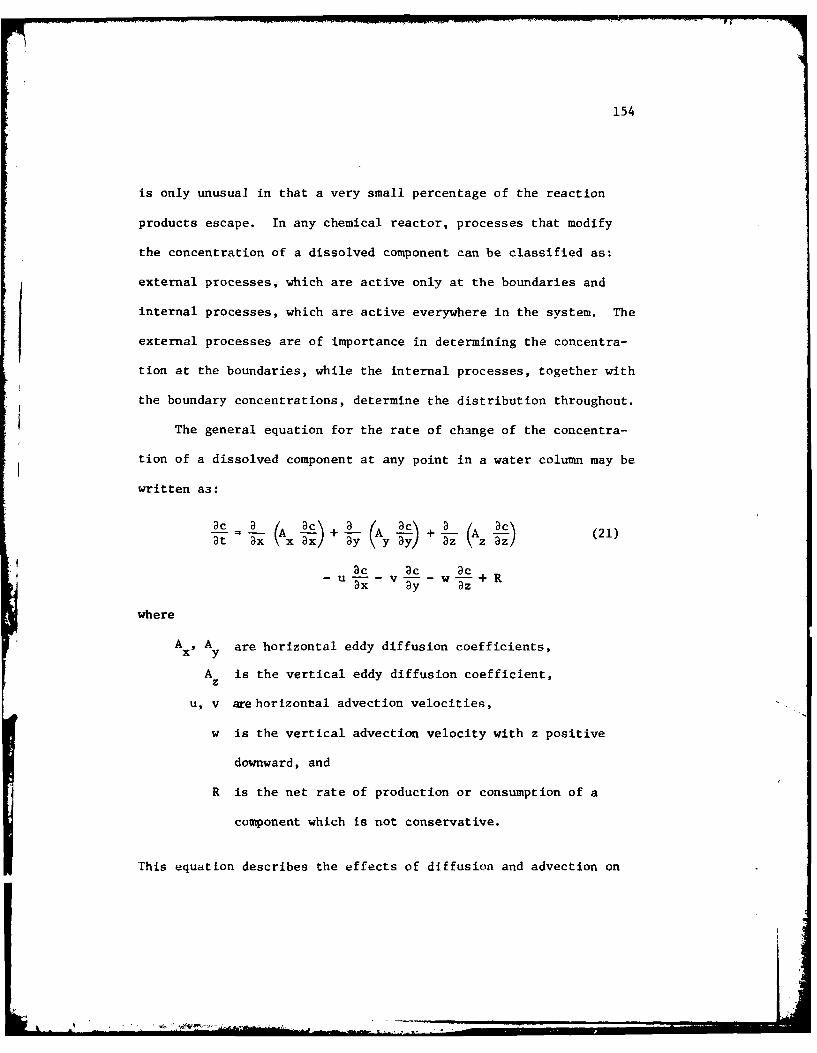
154

is only unusual in that a very small percentage of the reaction

products escape. In any chemical reactor, processes that modify

the concentration of a dissolved component can be classified as:

external processes, which are active only at the boundaries and

internal processes, which are active everywhere in the system. The

external processes are of importance in determining the concentra-

tion at the boundaries, while the internal processes, together with

the boundary concentrations, determine the distribution throughout.

The general equation for the rate of change of the concentra-

tion of a dissolved component at any point in a water column may be

written as:

at = a A x - L) + - L A a + -L A z - Lc (2 1 )

ac ax~ ac ay ( 3c) 3a 3c

Dc ac Dc! - U~~x -Vy - -z+R

where

Ax, Ay are horizontal eddy diffusion coefficients,

A is the vertical eddy diffusion coefficient,z

u, v are horizontal advection velocities,

w is the vertical advection velocity with z positive

downward, and

R is the net rate of production or consumption of a

component which is not conservative.

This equation describes the effects of diffusion and advection on

155

the local time rate of change, -, of a nonconservative solute

whose concentration, c, is changed chemically or biologically at

rate R.

In the chemical reactor that is the Orca Basin, organic ma-

terial raining down from the surface provides the fuel for the

diagenetic reactions given in Table 12. The processes of decom-

iI position in the Orca Basin are no different than in other anoxic

basins, but the high salt content of the water can have a great

influence on reaction rates and mechanisms. Eq. 22 also applies

to the Orca Basin, but rates of advection, diffusion and reaction

may be slower in this dense, hypersaline environment than in other

anoxic environments.

It will be argued in this discussion that the processes of

decomposition in the Orca Basin are no different than in other

anoxic environments, only slower. Briefly summarized the evidence

for reduced microbial activity in the Orca Basin is

(i) The presence of fronds of Sargassum seaweed in deep

cores. Kennett and Penrose (1978) have noted that this

type of preservation has never been observed before in

the deep ocean.

(2) A comparison of the initial sulfate gradients between

the Orca Basin and the basin next to it indicates that

sulfate is not as rapidly reduced in the Orca Basin

sediments.

156

(3) The isotopic composition of carbon dioxide and methane is

unusually light (relative to PDB standard) in the Orca

Basin. Sackett et al. (1979) suggested that the isotop-

ically light methane was the result of an unknown lighter

source material. However, slower rates of methanogenesis

would produce greater fractionation and could account for

the observed 613C values starting from the organic ma-

terial found in the brine.

(4) No pyrite is found in the Orca Basin sediments. If there

is only a slow production of sulfide in the Orca Basin,

the high iron levels would rapidly remove the sulfide

from solution and inhibit the continued reaction of

metastable iron sulfides to pyrite. Metastable iron

sulfides are found in the Orca Basin sediments, pyrite

has not been found.

Overall Effects of Decomposition

Organic matter in the marine environment has an ideal C:N:P

ratio of 106:16:1 by atom which is close to the statisLical aver-

age of planktonic material, the primary source of organic carbon

to the marine ecosphere. Anaerobic decomposition of this organic

matter can be expressed by the reactions in Table 12. The most

important reaction is sulfate reduction, given by the equation:

..... .......... .. r

157

(CR20)1 06 (NH3)1 6 3P0 4 + 53 SO - (22)

106 CO2 + 53 S + 16 NH 3 + 106 H20 + H3 P04

This reaction yields mole ratios for CO 2:S :N 3:H3 PO4 of 106:53:16:1.

Methane production during anaerobic decomposition will alter the

ratios predicted by this model by either liberating or consuming

carbon dioxide. Richards et al. (1965) proposed that one repre-

sentation of methanogenesis might be

(CH20) 10 6 (NH 3)16 R3PO 4 -O (23)

53 CH4 + 53 CO2 + 16 NH3 + H3 PO4

yielding mole ratios for CO 2:CH 4:NH 3:H 3PO 4 of 53:53:16:1 for the

products. This reaction would alter the ratios predicted by Eq.

7 by an amount dependent upon the quantity of methane produced.

In the anoxic waters of the Orca Basin, the average concentrations

observed for excess decomposition products are 2.28 mmol-liter-1

for rO 2 , 0.7 mmol-liter- I for CH4 (Sackett et al. 1979), less than

1 umol-liter for S, 500 Umol'liter for NH3 and 60 imol-liter

for P04 3 (this study). These values result in AC02 :CH :N :R PO44 2 4 3* 34

mole ratios of 38:12:8.3:1, far different than predicted by

Richard's (1965) model.

How can these differences be explained? It is doubtful that

these differences can be accounted for by compositional differen-

ces between Gulf plankton, and the world average planktouic ratios.

158

Plankton falling through the water column decomposes into par-

ticulate organic matter (POM). The POM in the deep water should

have the same characteristics as the plankton debris which reach

the bottom. Particulate organic carbon (POC) and particulate or-

ganic nitrogen (PON) have been reported by Fredericks (1972), in

both surface waters of the Gulf and at depth. The average values

he measured for POC and PON at the surface, and at 200 to 2200 m,

are shown in Table 16. When converted to a mole carbon and mole

nitrogen ratio, the C/N ratio in surface waters was 3.62 and in-

creased to a deep water C/N ratio of 7.78. The average of C/N

ratio for the model of Richards (1965) is 6.6, while the ratio

of excess carbon (CO2 + CH4 ) to nitrogen (NH3 ) in the Orca Basin

is 6.0. Considering variations in Fredericks' (1970) data with

depth all of these ratios are approximately the same.

Since the excess carbon to nitrogen ratio in the Orca Basin

approximates the theoreticdl ratio, there must be excess phos-

phate in the brine (brine PO4 = 60 Umol-liter- ). Phosphate could

be added to the brine from organic matter decomposition or by in-

put of phosphate associated with the brine coming from the LouAnn

salt, from which the Orca brine originated. Unfortunately, a

detailed study of phosphorus content in natural solution brines

has not been made. Of the few brines that have been analyzed,

most have contained less than 1 mg.liter- (Collins 1975). For

phosphorus, I mg'liter - I is equal to 32 mmol'liter- I .

I L I•, =- ... ll

159

u -H

0 uw$4 0

0 o3';a

to

0

m00

0 44-4 0 0~

V -40 L

0C1

'44u003

$3 (7 : 1 a

.414 U -.

b 0

03 0aa

L)

0 030'44

0to

160

The excess C/N ratio in the brine can be used to calculate the

predicted phosphate from anaerobic decomposition alone. Using the

brine C/N value of 6.0, the decomposition-produced phosphate would

be 27.8 imol.liter- I . This value would give a C:N:P ratio of

106:18:1, which is very near the predicted values from Richard's

model. This calculation suggests that there is an excess 32 umol"

liter - I of phosphate in Orca Basin. Considering the high phos-

phorus content of natural brine, the excess could be from the

original brine that entered the basin before any decomposition of

organic matter had occurred.

Microbial Activity in the Orca Basin

Distributions of the reduced species in the brine are con-

trolled either by in situ processes within the brine and sediment

and/or by the evaporite dissolution and migration of the brine into

the basin. Since the brine originates from solution by sea water

of a near-surface salt deposit within the basin, the reduced gases

should be controlled primarily by in situ processes within the

brine, after migration into the basin. The inflowing brine should

have initial reduced gas concentrations similar to overlying sea

water, as was shown for argon and nitrogen. Thus biological acticn

by anaerobic bacteria in the Orca Basin brine must produce the

concentrations of reduced species that were observed.

161

LaRock et al. (1979) have reported that ATP concentrations and

uridine uptake show an increase in magnitude above the brine inter-

face, followed by a decrease below the interface into the anoxic

zone. Substantial ATP increases were found further down in the

anoxic zone. As in other anoxic environments, the bacterial popu-

lations required to mediate the decomposition of organic matter are

present in the hypersaline waters of the Orca Basin. One might

expect the high salt content of the Orca Basin to inhibit microbial

activity. However, the observed ATP levels (3-15 ng ATP-liter-I )

indicate a larger bacterial population than in the overlying deep

-1Gulf waters, where values from 1-3 ng ATP'liter were observed

(LaRock et al. 1979). This large bacterial population is probably

associated with the high concentration of dissolved organic carbon

(3.5 mg C-liter- 1 ) and particulate organic carbon (70 pg Cliter

- )

observed in the brine (Sackett et al. 1979). Although the total

bacterial biomass is larger in the brine than in the deep Gulf, one

must consider the inhibitory effects of salt on the reaction rates

during bacterial decomposition.

Unfortunately, bacteria activity at high sodium chloride con-

centrations has received limited attention in the literature.

Larsen (1967) and Kushner (1968) have reviewed the literature on

halophilic bacteria and noted that they do not exclude salts, but

have an internal environment as high in ionic strength as their

external environment. Many bacteria are faculative halophiles,

162

and the sulfate reducers, methanogens, and other anaerobes

have probably accomodated themselves to the Orca Basin brine well

enough to produce or consume the reduced gases observed. Like

increasing pressure or decreasing temperature, the increasing salt

content of a solution will reduce the rate at which microbes per-

form their metabolic activities (Kushner 1978). Most bacteria

in hypersaline waters grow slowly, with mean generation times of

7-15 hours at 37*C (Kushner 1968), compared with generation times

of less than an hour for bacteria at sea water salt concentra-

tions and 37*C. The large concentrations of biogenic methane in

the Orca Basin (750 Umol.liter- 1, s3C = -74*of.), relative toCH4

other anoxic basins, and the evidence of sulfate reduction in the

sediments suggests that anaerobic bacteria are able to tolerate

the hypersaline conditions and actively reduce organic material

even at 5.6*C, a temperature much lower than the 30-40*C preferred

by most halophilic bacteria. Their slower rate of metabolism in

the Orca Basin, however, has a profound influence on the composi-

tions of the decomposition products found there.

Another bacterially-mediated decomposition reaction must be

considered in addition to those presented in Table 12. That is

the process of anaerobic methane consumption during sulfate re-

duction. Although the process of methane oxidation under aerobic

conditions is well documented (Vary and Johnson 1967; Wertlieb

and Vishniac 1967; Quale 1972; Rudd, Hamilton and Campbell 1974)

163

and bacteria are known to anaerobically utilize hydrocarbons higher

than methane (Novelli and Zobell 1947; Rosenfeld 1947; McKenna and

Kalio 1965), the actual consumption of methane by bacteria under

anoxic conditions is not well understood. Davis and Yarbrough

(1966) have suggested that methane could be an additional carbon

source for sulfate-reducing bacteria, and Fuhs (1961) has shown

several reactions for anaerobic methane consumption that are

energy-yielding. Generally, the longer the carbon chain, the more

energy the bacteria can obtain.

Although bacteria prefer to use the energy source with the

highest potential, it appears that methane consumption can occur

during sulfate reduction. In studies of the anaerobic oxidation

14of C-labeled methane by the sulfate-reducing bacteria, Desul-

fovibrio desulfuricans, Davis and Yarbrough (1966) noted that

these bacteria can consume methane, although at a slow rate. The

following reaction was proposed by Fuhs (1961)

C + - .HS + HCO + 2H 0 (24)4 4 3 2

with the reaction having a free energy of -4.5 kcal'mole- . The

consequences of anaerobic methane consumption would be decreased

methane levels in the immediate vicinity of consumption, and an

increase in the 61 3C of the methane. Isotopically lighter methane

would be preferentially consumed.

164

Methane and Hydrogen Sulfide in the Brine

The concentration of methane in the Orca Basin is extremely

high when compared to other anoxic areas (Table 17). The methane

levels are over 100 times higher than the concentrations found in

any other anoxic sea water, except for the oil-related East Flower

Garden brine in the Gulf of Mexico (Brooks et al. 1979). The only

natural water with higher methane content is Lake Kivu, an east

African rift lake where Deuser et al. (1973) reported finding a

methane concentration of 22 mmol-liter- . The high methane levels

in the Orca Basin probably result from the inability of methane

produced there to easily escape from the brine.

The methane distribution across the brine-sea water interface

is extremely sharp, with almost a six order of magnitude increase

in methane concentration as the depth increases only 50 m. Such

a sharp gradient is indicative of very slow mixing processes. Thus

methane can probably be removed from the basin only by molecular

diffusion, a very slow process. The gas that bubbles out of the

brine at the surface has a large component of methane. Methane is

supersaturated by several hundred percent (at one atm). This

supersaturation is the result of methane production with little

removal. The methane is produced in the sediments and perhaps at

the brine-sea water interface.

It is the density structure of the Orca Basin (Fig. 9) which

effectively inhibits removal of methane from the basin. Due to

165

0.0

0 -n

y 1- 0 0 %D. C*C4 0 I 0 mI eC-)

0

coI

r.i uo V

Cd 04 -1 r4 0) -4 '0 r") -4

0 C;C 8 -

04 010

.0 C)- *0

o C4,- V n CD C

00

0 w 04-

0 0

oH 0 C14 a m0. ~ '~ =L -4r, OO

-S 41 4 m0! 1-4 04f

-I C0 q

o 00 014-b 4c L-

U .. ta fP% %D 0- C'4 C'4 LQ 0

W~ 0 0- .-H- N. -, A41 Zo 0) " N

0d Enr. 90 0 ~ -,4 M .0W0. W. ('4 -, a- po ccU . C:M w 0

-4 - C o En ' '-.-4N '4 -

go1- p-. u~ v0 a

04 en 0T0n0 00

166

its stability (Table 5), the residence time of brine in the Orca

Basin must be longer than in other anoxic basins. Sackett et al.

(1979) found a 614C value for the total CO2 in the brine of

-501 0/00. This figure would imply an age of one half-life of 14C,

or about 5700 years. This residence time is much longer than for

other anoxic basins. There is much uncertainty in the 14C age,

however, due to a lack of knowledge of the 14C content of carbon

compounds that entered the basin with the brine. Addy and Behrens

(1980) used sedimentological data and 14C measurements of the car-

bonate in the sediments to calculate an age for the initial input

of brine into the Orca Basin. They determined that the brine began

flowing in to the basin 7900 years ago, a date even older than the

age from the 14C measurements of Sackett et al. (1979). The age of

Orca Basin water is greater than 800-year deep water residence

time for the Cariaco Trench (Fanning and Pilson 1972) or the 2000-

year residence time for bottom water in the Black Sea (Ostland 1974).

Unlike methane, the concentration of hydrogen sulfide in the

Orca Basin brine (Fig. 36) is much lower than in other anoxic

basins such as the Cariaco Trench or the Black Sea (Fanning and

Pilson 1973; Brewer and Spencer 1974). Except at the brine sea

water interface, sulfide is below the detection limits of the

molybdenum blue technique used in this study (Cline 1969). In the

167

Black Sea at 2000 m, both methane and hydrogen sulfide are observed

in high concentrations (Degens and Ross 1974). In the hot

Red Sea brine at 2050 m, methane is present (Burke et al. 1980)

but hydrogen sulfide is absent. There is little evidence that

significant sulfate reduction is taking place in the Red Sea brine

(Craig 1969). It can be argued that the rate of sulfide produc-

tion in the Orca Basin is not sufficient to maintain a high dis-

solved sulfide level, due to the presence of iron with which it

precipitates as metastable iron sulf ides. Alternately, it has

been suggested (Trabant and Presley 1978) that sulfate reduction

proceeds normally in the Orca brine, and there is simply a large

influx of iron from the sediments which is controlling the sulfide

levels in the brine. This discussion will show that the rate of

sulfate reduction is slow in the Orca Basin, and that reduced

sulfur species are completely removed from solution by reactive

iron. As such, the available sulfur is rapidly depleted from so-

lution before any conversion of FeS to FeS can occur, by the2

reaction

Fe So0- s. FeS - 4 FeS2 (25)

Addy and Behrens (1980) noted that there is no pyrite in the

Orca Basin sediments.

Sulfate reduction is occurring in the Orca Basin. The sul-

fate in the pore waters decreases to zero at a depth of f ive to

168

seven meters in the sediment (Sackett et al. 1979). Fig. 37 shows

a plot of the sediment data presented tabularly by Sackett et al.

(1979). The open circles represent the actual sulfate profile that

they observed. Also shown are the chloride gradient and a predic-

ted sulfate profile (SO4, closed circles) that would be found if

sulfate were diffusing down through the sediment at the same rate

as chloride, with no sulfate reduction. From the differences in

the actual and predicted sulfate profiles, it is obvious that sul-

fate reduction is occurring in the Orca Basin sediments. The

presence of hydrogen sulfide at the interface with the oxygenated

Gulf of Mexico (Fig. 36) water also shows that sulfide is being

produced there. However, the absence of H2S in the brine itself

may indicate that little sulfide is being produced in the anoxic

waters or if so, it is rapidly removed. The only appreciable sul-

fate reduction is probably occurring at the interfaces, the sites

of highest reactivity.

Although it is difficult to obtain rate data from concentra-

tion profiles alone, enough information is available about sulfate

profiles worldwide to gain some insight into rates in the Orca

Basin. The basis for the following discussion follows the review

of Goldhaber and Kaplan (1974) on worldwide sulfate profiles and

the more recent paper of Berner (1978). Both of these papers dis-

cussed i correlation between the sedimentation rate and the sul-

fate reduction rate, or the initial sulfate gradient in the near

surface sediments.

169

0-~ 0)

0 - <<o 0J. -1

C) z z-0 9

E O \O 0 4141c

0 I-J /4 / '

0 0 $)

0-~4- 00)- < 9

w - 00 / - 0

,- (4) 0L) (n00

-l co- vt 4-4CN 0W

44 4

ww E 010 '41

- W o Q)

'0 0

41) 41

E W 0\13 Z 0 0) 'a

(sia~dw aidi

170

Berner (1978) has shown that the log of the slope of the sul-

fate profile in marine sediments is directly correlated with the

log of the sedimentation rate. Also the rate constant for sulfate

reduction is directly correlated with the rate of sediment depo-

sition. This trend has been shown to apply to diverse environments

from nearshore sediments to abyssal Pacific sediments sampled during

the Deep-Sea Drilling Project. The actual sulfate sediment profile

in Fig. 37 (data from Sackett et al. 1979) has a slope of

-i0.053 mM SO4-cm The sedimentation rate in the Orca Basin has

been determined by Addy and Behrens (1980) to be 61 cmka- 1

Approximately 21 cm.ka- I of this sedimentation is attributable to

the preservation of excess carbonate material, as a result of the

anoxic hypersaline conditions which exist in the Orca brine. Tomp-

kins and Shephard (1979) estimated a sedimentation rate of 100 cm-

- However, the core that they used for making this estimate

was taken in the smaller lobe of the Orca Basin and had evidence

of slumping, which would cause their rate to be high.

Taking the rate versus rate hypothesis one step further,

Berner (1978) showed that there is a positive correlation, and a

very predictable one, between the sedimentation rate and the rate

of sulfate reduction. This point was also well illustrated by

Goldhaber and Kaplan (1974). Goldhaber and Kaplan (1974) concluded

that, besides temperature and pressure (which effect all reactions),

the rate of sulfate reduction is dependent upon:

171

(1) total organic carbon preserved in the sediment

(2) the state of complexing of the organic matter

(3) availability of organic matter for biogenic degradation

(4) the environment of deposition

(5) the sedimentation rate.

They noted that factors 1, 2 and 3 are directly influenced by fac-

tors 4 and 5, and that there was a direct relationship between the

rate sulfate reduction and the rate of sediment accumulation.

Considering factor 1, Sackett et al. (1979) noted that the percen-

tages of organic carbon in Orca sediments are higher than for nor-

mal shelf and slope sediments. According to Goldhaber and Kaplan

(1974) this would result in higher sulfate reduction rates.

From a comparison of the sulfate reduction rates in the Orca

Basin with those in the small basin next to Orca, it can be shown

that the rate of sulfate reduction is slower in the Orca Basin,

relative to the smaller basin and to other areas of similar sedi-

mentation rate. The sulfate profile in the small basin next to

the Orca Basin has been measured by Bernard (1978). A comparison

of the initial sulfate gradient, OSO4 /jz)o, of the small basin

(0.11 mM So4 -cm - ) with the Orca Basin (0.053 mM SO4 -cm

- ) indi-

cates that the gradient is steeper and thus the rate of sulfate

reduction in the other basin is greater than the Orca Basin. Yet

the sedimentation rate in the Orca Basin is at least 20 cm-ka-

higher. The sulfate reduction rate should be higher, not

7AAI03 536 TEXAS A AND M UNIV COLLEGE STATION DEPT OF OCEANOGRAPHY F/B 8/~4KOC0EMISTRY OF DISSOLVED *AtES IN THE HYPERSALINE ORCA BASIN. (U)

IDEC SO0 DA WIESENURO N00O475COS537

UNCLASSIFIED TANU-REF-8-1IVT NL13 m~EhhE

172

lower in the Orca Basin. If the hypothesis of Berner (1978) were

applicable to this area, the sedimentation rate in the small basin

next to Orca should have a sedimentation rate twice as fast as

the Orca Basin. The two basins are separated by only 25 km. Thus

it is reasonable to assume that the same material being deposited

due to sedimentation is available to each basin.

The major factor causing the differences in the initial sul-

fate profiles and sulfate reduction rates of the two basins must

be the high salinity brine in the Orca Basin. The hypersaline

water in the Orca Basin does not completely inhibit sulfate

reduction per se, but the rate of sulfate reduction seems to be

decreased as a result of the high salt content, creating a smaller

sulfate gradient.

The idea that the rate of microbial activity is slower in the

Orca Basin than in other anoxic environments is consistent with

the effects of salt stress on microbes (Kushner 1978). A reduced

microbial activity rate might also explain some seemingly anomalous

carbon isotope data that has been reported for the basin sediments

(Sackett et al. 1979). It should be remembered that the pro-

duction of methane from organic material is a two-step process.

One suite of bacteria breaks down organic matter into small organic

molecules and carbon dioxide. Methanogenic bacteria then reduce

these compounds to methane. The sediment methane data taken

from Sackett et al. (1979) are shown in Fig. 37. They

173

explained the data by suggesting that the source material for the

carbon in the Orca Basin must be isotopically lighter than could be

accounted for by the isotopic ratios of the products (CO 2 and CH 4)

they observed. They further suggested that the ultimate source for

the isotopically light organic carbon in the basin might be methane

migrating upward from a deeper reservoir. This methane would be

oxidized to CO 2and subsequently reduced back to methane, yielding

the isotopic balances observed. Several mass balance calculations

from mixture models suggested that the source carbon for the source

organic material in the basin needed to be -42o/.. to account for

values observed.

An alternate argument can be made, if one considers that the

rate of sulfate reduction and methane production are lower in this

unusual environment than in other areas where methane has been

measured and classified isotopically (Bernard 1978). Most of

the organic material found in the sediments of the Orca Basin had

an isotopic composition essentially the same as other sediments

in the region (6 1 3 C g 22*/eo.) . Some depths, however, had isotop-

ically light organic carbon, which may represent slumped sediments,

originally deposited in estuarine environments during the Pleisto-

cene (Sackett et al. 1979). For this discussion, I assume that the

normal slope organic carbon (613C = -22*/..) is the source carbon

for methane and carbon dioxide found in the basin water and sedi-

ments. The normal isotopic fractionation for methane produced

during this process varies as a function of several factors,

174

including isotopic content of the source material (Bernard 1978)

and temperature of reaction (G-ames et al. 1978). A decrease

in temperature increases fractionation, perhaps by decreasing

the reaction rate, thus allowing increased bacterial selectivity

of the source carbon. The idea of enhanced isotopic fractionation

at reduced reaction rates has been suggested in several studies.

Kaplan and Rittenberg (1964) showed that isotopic fractionation

32Sv.3 S) during sulfate reduction was directly influenced by

the rate of sulfate reduction, The magnitude of the separation

between sulfur isotopes was inversely proportional to the rate

of sulfate reduction. The same effect should be true for methane

carbon fractionations.

En reality, factors other than reaction rate are responsible

for changes in fractionation. Fractionation in microbial systems

occurs along enzymatic pathways, due to the preferences of trans-

port enzymes for carbon-12 atoms. Under slower reaction rates, or

salt stress, the enzymatic pathways may change or the effect of

various back reactions (with different fractionations) may become

important. These complex systems are difficult to investigate.

Thus the simplistic idea of greater fractionation at reduced rates

has been generalized to describe the overall effects of these

processes.

Also important for this discussion is a consideration of the

organic material used during sulfate reduction. It is now well

175

established that methane can be consumed during sulfate reduction

in natural environments (Barnes and Goldberg 1976; Reeburgh 1976;

Martens and Berner 1977; Murry et al. 1978). However, methane is

not the preferred substrate for sulfate reducing bacteria (Rosen-

feld 1947; McKenna and Kalio 1965). Sulfate reducers derive more

energy from consuming organic material with a carbon chain length

greater than one. In one study where the sulfate reduction rate

was low, no methane was consumed (Sorokin 1957). Methanogenesis

in the Orca Basin sediments would produce isotopically light

methane which would remain unaltered during slow sulfate reduction.

If the rate of methanogenesis is very slow in the Orca

Basin sediments, one would expect a greater fractionation than has

been observed in other environments. Laboratory fractionation

experiments (e.g., Games et al. 1978) are performed under conditions

where reaction rates are relatively high, so results can be ob-

tained rapidly. Games et al. (1978) found fractionation factors

of 1.044 to 1.061 for methane produced in laboratory cultures. If

they had used the carbon dioxide in the Orca Basin as the source

material, these fractionations would produce methane in the range

-71 0/., to -88 %o.. If their methane production rates had been

slower, the fractionation might be even greater. Greater frac-

tionation would produce methane lighter than -88 o/., and could

produce the -105 %/oo that was measured by Sackett et al. (1979).

- '..---

176

The idea of the salt in the basin being the factor which re-

duces the rates of methanogenesis and sulfate reduction is para-

mount to this discussion. In the Red Sea brines, Watson and Water-

bury (1969) attempted to culture sulfate reducing bacteria in brine

at various sodium chloride concentrations. They found that there

was a reduction in the rate of sulfate reduction with the increas-

ing salinity and no sulfate reducers could grow at salinities

greater than 125 0/.. Some sulfate reduction is taking place in

the Orca Basin sediments, as evidenced from the sulfate profiles

shown in Fig. 37. However, the rate of sulfate reduction may

not be constant throughout the entire sediment column. Micro-

bial activity may be more rapid in certain areas. One of these

areas would be the sediment-water interface zone, where the

most labile organic material reside. It has often been noted that

very rapid sulfate reduction rates occur in a very thin zone near

the sediment-water interface (Berner 1972; Sweeney 1972; Goldhaber

and Kaplan 1974). Rapid sulfate reduction at the sediment-brine

interface could account for both the decrease in methane and the

increase in 13C of the methane in the near surface sediments

(Fig. 37). This is the same type of response that is found in

coastal sediments in the Gulf of Mexico (Bernard 1978) with

methane concentrations decreasing and becoming isotopically heavier

near the sediment water interface. Significantly, in the Orca

Basin, the heaviest methane is found at the sediment-brine

interface.

177

Methane consumption during more rapid sulfate reduction at the

sediment-brine interface would also account for the fact that

methane is isotopically heavier in the water column (613C = -73.5

Yoo) than in the sediments (613C = -85 to -105Y 00 ). The lighter

methane would be consumed at the interface leaving the isotopically

heavier methane to diffuse out into the water column. Conversely,

away from the sediment-brine interface, where microbial popula-

tions would be lower (Zobell 1942), rates of sulfate reduction and

methanogenesis may increase with depth. This would happen since

there is a decreasing chloride gradient with depth. The data in

Fig. 37 are consistent with this explanation. 1 3C of the methane

would increase with depth in the sediment as the sulfate reduction

rates increase or as heavier organic carbon is encountered for

use in methane production.

In the water column, there is too much scatter in the methane

and 613CH4 data (Fig. 30) to determine the processes affecting

the methane distribution there. Methane is obviously consumed at

the brine-sea water interface by aerobic oxidation, but there are

no other noticeabletrends in the deeper data. The high salinity

brine in the Orca Basin is fairly well mixed, as was discussed

in Chapter II. This mixing is obvious in the methane distribu-

tion. In summary, the observed methane profile in the high sa-

linity brine results from production and consumption in the sul-

fate containing sediment and brine, with only limited loss of

7 7t;

178

methane from the brine, probably by diffusion across the brine-

sea water interface.

Mechanisms of H S Removal2

Having concluded that sulfate reduction is an active process in

the Orca Basin, one must ask where the produced sulfide goes. Free

sulfide that is produced is rapidly removed to the sediments as

iron sulfide. The iron sulfides that are formed, however, are not

pyrite (FeS2) but metastable iron sulfides such as greigite (Fe3S4)

and machinawite (FeS) among others (Addy and Behrens 1980). Ber-

ner et al. (1979) have noted that the formation of pyrite is di-

rectly influenced by the presence of available sulfur. The conver-

sion from metastable iron sulfides to pyrite occurs by the addition

of sulfur to FeS (Rickard 1975), and not by the removal of iron.

A generalized reaction is (Berner et al. 1979):

Fe S + 2H2S 3FeS + 4H + 4e (26)3 4 2 -2

Metastable iron sulfides such as greigite and mackinawite are

thermodynamically unstable relative to pyrite, in the presence of

H 2S (Berner 1972). Thus the absence of pyrite in the Orca Basin

sediments is indicative of the influence of iron in rapidly re-

moving the free sulfide from solution.

The 30-33 pmol-liter concentrations of iron that were

found in the brine (Fig. 36) are two orders of magnitude higher

179

than the iron values reported for the Black Sea (Brewer and Spen-

cer 1974). In the Black Sea, the hydrogen sulfide concentration

is 300-500 pmol*liter- I and iron sulfides are known to precipitate,

as evidenced by their concentrations in the sediment (Berner 1974).

The high iron concentration in the Orca Basin has caused almost

complete sulfide removal from the Orca Basin waters. With a slow

input of microbial sulfide to the brine, the iron that is entering

the brine from sediment reaction or from decomposing plankton

precipitates all available sulfide. In the Orca Basin, sulfide is

the limiting species in FeS precipitation.

Other Light Hydrocarbons in theBrine

The production of methane by fermentation shows (Thayer 1931;

Stadtman and Barker 1951) that fatty acids are not decarboxylated

during methanogenesis and regardless of the length of the carbon

chain no hydrocarbons higher than methane should be produced. In

spite of this conclusion, C2 and C3 hydrocarbons are found in

many anoxic environments (Table 17) and are probably produced by

bacteria (Bernard 1978). In the Orca Basin, ethane concentrations

as high as 1300 nmol. liter -1 were observed, over 50,000 times the

concentration found in the deep Gulf water. Propane was also ob-

served just above the interface at a level of 0.4 nmolliter- 1 ,

-

180

almost 20 times the deep Gulf concentration. This type of increase

in non-methane gaseous hydrocarbons has also been observed in the

Cariaco Trench (Linnenbom and Swinnerton 1969), the Black Sea

(Hunt 1974), the Red Sea brine and Lake Nitinat (Swinnerton and

Linnenbom 1969) and other anoxic waters (Table 17). Bernard (1978)

has shown that these hydrocarbons are also found in anoxic sediments.

He attributed these gases to bacterial production. Biological

production of C2 and C 3 hydrocarbons has yet to be satisfactorily

explained. The generally accepted mechanisms of anaerobic decompo-

sition (Berner 1971) would preclude microbial production of ethane

and propane. Gaseous hydrocarbons higher in molecular weight than

methane are normally the result of petroleum production. However,

the depth distribution of ethane in the Orca Basin (Fig. 30)

indicates an origin similar to methane: biogenic.

Methane at the Interface

The maximum in methane, ethane, and propane above the brine-

sea water interface was not entirely unexpected. The microbial

biomass distribution (LaRock et al. 1979) exhibits a pattern above

the interface similar to the observed methane distribution. The

two may be associated. The increased density of the brine, rela-

tive to the Gulf water, would cause particles falling to the sea

floor to be temporarily interrupted in their journey. They would

rest at the interface until they reach isotonic balance with the

t ,.*-

181

higher salinity brine. Only after particle densities reach the

level of the next brine layer would they settle below the inter-

face. An increased microbial biomass would be expected to corre-

late with a great number of particles. Degradation of particles

at density interfaces has been proposed to account for the near

surface methane maxima that have been observed in many areas of the

world oceans (Brooks et al. 1980). The main difference here is the

depth of maxima above the Orca Basin. This methane maximum is

deeper than any previously reported.

The methane depth distribution above the brine interf ace is

also consistent with the concept of methane consumption in oxy-

genated waters. Rudd et al. (1974) have shown that, in oxygenated

waters, methane consumption rates are the highest where the oxygen

values are minimal. They made this observation from determinations

of methane consumption rates in oxygen minimum layers of several

Canadian Shield lakes. As can be seen in Fig. 32, the methane

maximum above the interface is in water that has a decreasing

oxygen gradient, but where oxygen is still present. This would

rule out possible methane consumption during sulfate reduction,

since sulfate is not reduced while oxygen is available. Oxygen,

from molecular oxygen, must be the oxidizing agent in any

j microbial methane consumption above the interface.

It must be assumed that interface methane, and presumably

ethane and propane, being produced are produced in anaerobic

182

microenvironments. These microenvironments in the aerobic water

column need not be entirely sulfate depleted as Oremland (1975) has

reported small amounts of methane production (1.81 to 1.86 pmol-m - 2.

hr- ) in sulfate-rich marine sediments in the Florida Keys. Methane

may be produced throughout the entire interface region in these

microenvironments, with a constant production rate. This idea,

plus surface venting, has been proposed to account for the methane

maxima in some surface waters (Scranton and Brewer 1977). If this

were the case, the decrease in methane below the maximum would

result from an increased rate of methane consumption in the zone

where the oxygen concentration is the lowest. The increased

consumption at low oxygen concentrations observed by Rudd et al.

(1974) may not have real implications for consumption vs. oxygen

level. Not coincidentally, the largest population of methane

consuming bacteria would also be found in the low oxygen region,

since it is closest to the methane source.

N 20 Consumption During Denitrification

In the sequence of organic decomposition which proceeds from

oxygen consumption to carbon dioxide reduction, oxidized nitrogen,

especially NO and NO-, is consumed by various denitrifying3 2

bacteria and converted to gaseous nitrogen compounds, mainly

nitrogen gas and ammonia. The geochemistry of molecular nitrogen

gas was discussed in Chapter III. The presence of the 500 ilmol-

183

-1liter of ammonia can be accounted for based on organic decomposi-

tion, using the Orca brine excess carbon to nitrogen ratio as a

starting point. In measurements of nutrient regeneration in the

anoxic sediments, Martens and Berner (1977) show a large NH3 pro-

duction, but note very emphatically that there was no production

of molecular nitrogen in the sediments. The same is true for the

high salinity, anoxic brine in the Orca Basin. Yet, Weiss (1969)

has suggested that there is nitrogen production in the Red Sea

brines, presumably from decomposition of organic nitrogen. This

process causes both the high N2 concentrations and the high N2/Ar

ratios that he observed there.

Denitrification is nearly complete in the Orca Basin waters.

All NO3 and NO2 have been reduced and the main repository for

reduced organic nitrogen is ammonia. Nitrous oxide (Fig. 34)

decreases from over 15 nmol-liter- above the brine to only a

trace amount in the brine. Thus, almost all the N 20 has been con-

sumed during denitrification in the Orca Basin waters. Cohen and

Gordon (1978) have demonstrated that N20 can be consumed not only

in completely anoxic waters such as Saanich Inlet, but they noted

biochemical N 20 was consumed by marine denitrifying bacteria.

Barbaree and Payne (1967) and Payne et al. (1970) found that cul-

i tures of Pseadomonas perfectomarinus can use N 20 as a terminal

oxidant and reduce it to N . Matsubara and Mori (1968) also

show that anaerobic cultures of P. denitrificans can reduce N 20 to

__

184

N 2with lactate as the terminal hydrogen donor. Although N 20 has

been depleted in the Orca brine and increased N 2concentrations

have been measured there (Fig. 26), it seems unlikely that N 2 pro-

duction from N 20 is significant there. For the organic nitrogen

(which is eventually converted to ammonia) to participate in the

nitrogen production, it must first be oxidized to NO0 In anaer-

obic waters, however, there is little reason to believe that this

type of reaction would occur, and if so that the NO- would then be3

convrte to 2*Thepossibilities of a two step production of

N 2from ammonia in the oxygen step region have been discussed

earlier.

In summary, the decomposition processes that produce the re-

duced gases in the Orca Basin are no different than in other anoxic

environments. The rates are just slower. A combination of the

slower reaction rates and the high stability of the brine in the

Orca Basin makes this environment an ideal laboratory for studying

the mechanisms involved in anaerobic decomposition. The isotopic

fractionations found there are the greatest reported to date, far

greater than could be produced in laboratory experiments over the

lifetime of a graduate student. An examination of the degree of

sulfur fractionation in this basin would prove valuable for better

understanding reduced gas biogeochemistry under hypersaline

conditions.

185

CHAPTER V

CARBON DIOXIDE AND THE CARBONATE SYSTEM IN

THE HYPERSALINE BRINE

The Orca Basin brine is basically a sea water solution that

has been saturated with sodium chloride (Table 3). Besides sodium

chloride, however, the most important compound in higher concen-

tration in the brine than in normal sea water is carbon dioxide.

Some carbon dioxide probably entered the basin with the inflowing

brine, but most excess CO2 was produced in the basin itself. The

isotopically light carbon dioxide (61 3C = -16.4o) in the brine

(Sackett et al. 1979), compared to the source Gulf water (613C =

0.3oo.), indicates that the excess carbon dioxide has a biogenic

source. Biogenic reactions which produce carbon dioxide have been

discussed in the previous chapter (see Table 12). The effects of

hypersalinity in the Orca Basin on the interactions controlling

carbon dioxide system in the Orca Basin are considered here. The

previous chapters have been concerned with dissolved gases which

generally do not react with water. Carbon dioxide, on the other

hand, engages in a series of equilibrium reactions when it comes

in contact with water or sea water. These carbonate system re-

actions will determine the disposition of the biogenic CO2 added

to the brine from the anaerobic decomposition of organic matter.

186

Ionic interactions are important in defining the carbon

dioxide system. The total ionic strength of the Orca Basin brine

(4.10) is quite large relative to normal sea water (-0.7). The

ionic strength and ionic balance percentages of the ions in the

Orca Basin, sea water and several other brines are given in Table

18. Since the ionic strength of brines is so high, one would

expect their physical-chemical properties to be strongly influenced

by ionic interactions. Any physical-chemical effects would be due

both to the total ion concentration, as well as to the nature of

the ions which are important in the interactions in question.

Different ions participate to varying degrees in ion pairing

(Garrels and Thompson 1962). In sea water, there are interactions

between Na+, K+, Ca - , and Mg - with HCO , C03, and SO4 . Johnson

and Pytkowicz (1979) have recently calculated that Cl can also

form ion pairs in sea water to produce an NaCI complex. This pos-

sibility has interesting potential for the Orca Basin since the

ionic balance percentages of Na+ and Cl- are significantly higher

than sea water (Table 18). Pytkowicz and Atlas (1975) have shown

that knowledge of variations in solution composition are suffi-

cient to predict changes in buffer intensity which reflect vari-

ations in apparent dissociation constants of the carbonate system.

Thus the relative percentages of cations and anions in the Orca

Basin, as well as the total ion concentration, play an important

role in deciphering carbon dioxide interactions in the brine.

187

0

0)c

c-a

Iu en ~ I'D o C .II~ 0 cn%

0

co 04 000 0

41. 1-4

0W to IT n r- '.Q en44- CuO0 It M4 ( C14 r- cn1 .

U n a' 0 -I %0 Nl

0. C% 14

4. -2-i CC ! 4 '.0 cli

~0 mC

-1- a' C40O + '0

-H +d C a' C4~ C44.8 w u w. C L 'n gI f

4 c4 6 4 N

Cu C4

z '.0 C14 a' ON as

ua

-Hd U) o

Cu f'- 0000.- n

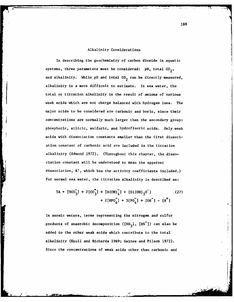
188

Alkalinity Considerations

In describing the geochemistry of carbon dioxide in aquatic

systems, three parameters must be considered: pH, total CO2 ,

and alkalinity. While pH and total CO2 can be directly measured,

alkalinity is a more difficult to estimate. In sea water, the

total or titration alkalinity is the result of anions of various

weak acids which are not charge balanced with hydrogen ions. The

major acids to be considered are carbonic and boric, since their

concentrations are normally much larger than the secondary group:

phosphoric, silicic, sulfuric, and hydrofluoric acids. Only weak

acids with dissociation constants smaller than the first dissoci-

ation constant of carbonic acid are included in the titration

alkalinity (Edmond 1972). (Throughout this chapter, the disso-

ciation constant will be understood to mean the apparent

dissociation, K', which has the activity coefficients included.)

For normal sea water, the titration alkalinity is described as:

TA = [HCO 3I + 2[C03 1 + [B(OH)4] + [Si(OH) 307] (27)

+ 2[HPO ] + 3[PO] + [OH-] - [H+ 1

In anoxic waters, terms representing the nitrogen and sulfur

products of anaerobic decomposition ([NH3 ], [HS ]) can also be

added to the other weak acids which contribute to the total

alkalinity (Knull and Richards 1969; Gaines and Pilson 1972).

Since the concentrations of weak acids other than carbonic and

189

boric are relatively low in sea water, they are generally excluded

from the total alkalinity. Boric acid contributes only a few

percent to the titration alkalinity of normal sea water. However,

it needs to be considered for precise alkalinity determinations of

normal oceanic samples.

In the Orca Basin, carbonic acid is by far the major contrib-

utor to the titration alkalinity. The dissociation constants

for acids other than carbonic acid are poorly known even for

normal sea water, and are non-existant for hypersaline solutions.

Thus, for my discussions of carbonate systems in the Orca Basin, I

have ignored all alkalinity components other than carbonic acid

and its dissociation products. This omission causes no concern

for borate, silicate, or phosphate. It may, however, be an in-

appropriate assumption with regard to NH3 . The ammonia level in

-1l3the Orca Basin is about 500 Umol.liter , or about 10% of the

total carbonate concentration. However, it is not the total

species concentration which determines the contribution to alka-

linity, but rather the weak acid contribution determined from both

the dissociation constants and the total concentration. For

ammonia, the contribution to alkalinity would be described as:

= [NH3] NH3 (28)3H

ANH 33 aH + M3(8

where AN 3 is the ammonia alkalinity, [NH3] is the total ammonia

concentration and K is the apparent dissociation constant forH3

190

ammonia. One can assume p = 9.2 (Sillen and Martell 1964),ammnia On cn asum pH3

which is the dissociation constant for infinite dilution, since no

equilibrium values are available even for sea water. Using the pH

of the Orca Basin (6.83), it can be calculated that the 500 umol-

liter- I of ammonia in the Orca Basin contributes only 2.13 peq.

liter- I to the alkalinity. Millero et al. (1979) calculated AT

to be 4750 Veq'liter-l, thus making the ammonia contribution in-

significant - if K is correctly assumed. For the anoxic water%3

of the Pettaquamscutt River, Gaines and Pilson (1972) assumed that

the total dissolved ammonia was equal to its alkalinity contribu-

tion. This assumption would require p I to be around 6.9 and may

be inappropriate. Yet, the dissociation constant for ammonia is

unknown. There is even some confusion as to whether the ammonia

contribution should be considered a weak acid (Gieskes 1974) or a

weak base (Knull and Richards 1969). Considering the uncertainty

as to how to treat the ammonia contribution to the alkalinity, I

have chosen to disregard it.

Carbonate System Interactions

Carbon dioxide which enters oceanic waters from the atmos-

phere, or from decomposition processes, participates in equilibria

which may be summarized by a generalized equation:

K' K .CO + HO0 H CO - CO_ + H + 20 C =+ 2H + (29)

2 2 .- 2 3-~-- 3 .-. 3

191

Associated with each step in this series is an equilibrium constant

which can be expressed in terms of thermodynamic activities of the

participating species. The basic equations necessary for quantify-

ing the interactions of carbon dioxide with its parent solution

are (Skirrow 1965):

+ [HCO3] First apparent dissociation

K' constant (30)1 [H 2 Co3I

K' 3 - Second apparent dissocia- (31)2 [HCO 3I tion constant

A =[HCO 2[CO - Carbonate alkalinity (32)

C = [HCO] + [HCO-3 Total dissolved carbon2 3 [ 3 (refers to inorganic

+ [CO2-] carbon) (33)

A= TB - Borate alkalinity (34)

where primes indicate that the constants are apparent dissociation

constants, brackets designate molar concentrations and aW. is the

activity of the hydrogen ion (see Table 19 for complete notations).

A detailed knowledge of the carbonic acid equilibrium system is

of considerable practical importance. In principle, it allows the

concentrations of various species (e.g. HCO3 , CO3 1 H 2CO3, and

total CO2 ) to be calculated by measuring any two of the parameters

192

Table 19. Notation for carbonate calculation.

a H activity of hydrogen ions, definedby pH f - log aH

K1 first apparent dissociationconstant of carbonic acid andpKf - log K1

K2 second apparent dissociationconstant of carbonic acid andpK2 f; log K 2

first apparent dissociation

constant of boric acid and

C total dissolved inorganic carbon

A 0titration alkalinity, initial

Ac carbonate alkalinity

T B Total dissolved boronconcentration

Aborate alkalinity

activity coefficient of thehydrogen ion where [H+] - aN

Y

Na normality of HCI used in titrations

An titration alkalinity at the ntht step of an HU titratin

I .. ' : 'i

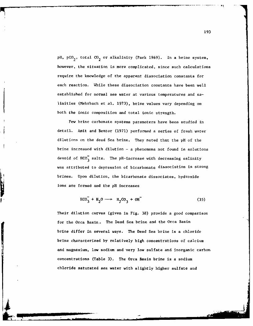
193

pH, p 29 total CO2 oraklnity (Park 1969). In a brine system,

however, the situation is more complicated, since such calculations

require the knowledge of the apparent dissociation constants for

each reaction. While these dissociation constants have been well

established for normal sea water at various temperatures and sa-

linities (Mehrbach et al. 1973), brine values vary depending on

both the ionic composition and total ionic strength.

Few brine carbonate systems parameters have been studied in

detail, Amit and Bentor (1971) performed a series of fresh water

dilutions on the dead Sea brine. They noted that the pH1 of the

brine increased with dilution - a phenomena not found in solutions

devoid of HCO 3salts. The pH-increase with decreasing salinity

was attributed to depression of bicarbonate dissociation in strong

brines. Upon dilution, the bicarbonate dissociates, hydroxide

ions are formed and the pH increases

HCO 3 + H 20- H 2 CO3 +OH (35)

Their dilution curves (given in Fig. 38) provide a good comparison

for the Orca Basin-. The Dead Sea brine and the Orca Basin

brine differ in several ways. The Dead Sea brine is a chloride

brine characterized by relatively high concentrations of calcium

and magnesium, low sodium and very low sulfate and inorganic carbon

concentrations (Table 3). The Orca Basin brine is a sodium

chloride saturated sea water with slightly higher sulfate and

194

pH

8.6

8.4

8.2 -

8.0-

7.8-

7.6-

7.4 -

7.2 - Dead Sea brineo Elat Sea water

7.0 a Mediterranean Sea water

6.8

6.6

S i I I I I I

300 200 100 50 30 20 10 4 2 1

Salinity (o/oo)Fig. 38. pH versus log salinity dilution curves for the

Dead Sea brine and two other waters (after Amit and Bentor1971).

• -Massa

195

calcium, a deficiency in magnesium and about twice the total in-

organic carbon as sea water. Thus two differences which will

cause varying carbonate interactions between these two brines are

the differences in ion interactions and in the total CO2 levels.

Sass and Ben-Yaakov (1977) have done a thorough study of the

carbonate system in the Dead Sea brines. They developed a gen-

eralized method to determine the alkalinity, total carbonate and

dissociation constants of any system. Applying this method to

the Dead Sea brines, they observed that as the salt content in-

creases, the dissociation constants also increase, resulting in a

consequential pH decrease. Their work confirmed the earlier con-

clusions of Amit and Bentor (1971) in this regard. More importantly,

their results showed that the chemistry of carbonate system in

hypersaline waters differ only in degree of interactions and not

in nature from the carbonate chemistry in less saline waters.

Thus, the carbonate system equations that have been developed to

describe sea water carbonate equilibria can also be applied to

hypersaline waters such as the Orca Basin brine.

The Orca Basin carbon dioxide system was investigated using

both the pH-dilution process of Amit and Bentor (1971) and the

titration techniques used by Sass and Ben-Yaakov (1977). Field

measurements were made of total carbon dioxide and pH. Laboratory

titrations of brine with HCl and NaHCO3 are also used to unravel

the carbonate system interactions. Treatment of the data reflects

196

a desire of the author to make comparisons between the Orca Basin

brine, the Dead Sea brine, and deep Gulf sea water. For this

reason, the calculation methodology involved is parallel to that of

Sass and Ben-Yaakov (1977).

Methods

Sampling

Sampling requirements for total CO2 are less stringent than

for other Orca Basin gases. This is true since the CO2 in the

brine is mainly tied up as bicarbonate and carbonate. Less than

one percent of the effervescing gas from the brine was CO Brine

samples were taken on several cruises for pH, total CO2 , and alka-

linity analysis. Both Niskin and Nansen bottles were used with

no obvious systematic variations between bottle types. pH samples

were transferred by gravity flow to 125 ml hard plastic bottles

which were allowed to overflow and then sealed with rubber stoppers.

pH values were measured (by Tonalee Carlson) as soon as the brine

had come to thermal equilibrium at 25*C.

Brine was sampled for total CO2 analysis using 12 ml

plastic syringes attached to the Nansen or Niskin bottles with

tygon tubing. A three-port Luer-tip stopcock was used to flush

the syringe so an air free sample could be obtained. Some samples

were also taken on cruise EN-32 using the all glass sample con-

tainers shown in Fig. 21. All samples were kept refrigerated

197

and in the dark until analysis aboard ship - usually within 12

hours.

Alkalinity analyses were performed in the laboratory, rather

than aboard ship. Samples for alkalinity titration were collected

in 300 ml glass bottles with plastic-on-metal crimp shut tops.

Each bottle was filled and about 100 ml of brine was allowed

to overflow. 20 ml of brine was decanted and one ml of a saturated

NaN 3 solution was added to each bottle to inhibit bacterial removal

of CO2. Samples for alkalinity titration were stored at 4*C and in

the dark until analysis in the laboratory at Texas A&M University.

Analytical Techniques

pH. The pH of the Orca brine was measured at 25C using

Beckman glass electrodes in conjunction with a Radiometer Model

PHM64 pH-millivolt meter. Millivolt measurements were made and

converted to pH by making the same measurements on three different

National Bureau of Standards (NBS) buffers of known pH, and calcu-

lating the brine pH using linear regression. Pykowicz et al.

(1974) have shown that operationally defined hydrogen ion activity

measurements (pX, where X = kaH and k represents the effects ofJH

liquid junction and asymmetry potentials) compare well with pH,

since k is almost unity.

The problem of electrode junction potential should be briefly

mentioned since previous studies (Ben-Yaakov and Sass 1977) had

*1

• m " " " t

| -- -

198

questioned the validity of pH measurements in hypersaline waters

of the Dead Sea brine (Amit and Bentor 1971). Like this study,

Amit and Bentor (1971) used conventional pH electrodes with in-

herent liquid junction potentials. Ben-Yaakov and Sass (1977) con-

structed a pH electrode without a liquid junction and made inde-

pendent measurements of the pH of synthetic Dead Sea brine. Their

measurements were strikingly similar to the values reported by

Amit and Bentor (1971). Their verification confirmed that the po-

tential problem resulting from the liquid junction in conventional

pH electrodes is not a significant factor in making pH measurements

in hypersaline solutions.

Total carbon dioxide. A gas chromatographic system which

uses the on-line gas stripping techniques of Swinnerton et al.

(1962) was used for total CO2 analysis. A schematic of the system

is shown in Fig. 39. One ml of concentrated phosphoric acid

was injected via a septum (S) into the glass stripping chamber

(GS). After all air had been stripped from the acid, a 6 to 12 ml

brine sample was injected into the stripper where the bicarbonate

and carbonate are converted to gaseous CO The CO2 is swept from

the stripper by a helium carrier gas flowing at 20 ml.min-1. The

gas is dried using either a 20 mesh drierite or 40/60 mesh silica

gel drying column (DC) and passed to a 40/60 mesh silica gel sep-

aration column (SiGel, 1.0 m x 0.64 cm O.D. stainless steel) at

500C for separation of air and CO2. The gas chromatograph used

199

V DC

PR AZFC

I .t ; ~BV."" O

GS

Fig. 39. Schematic presentation of the gas chromatographicsystem used to measure total carbon dioxide in the Orca Basinbrine. Acid is injected into the gas stripping chamber (GS)via a rubber septum (S) and followed by injection of the brine~sample. The helium (He) carrier gas flow forces the carbon

dioxide from the chamber through a drying column (DC) and intothe gas chromatograph. The carbon dioxide is separated fromair in the sample by a silica gel column (SiGel) thermostated

' at 500C. The carbon dioxide is measured with a thermal con-1ductivity detector (TCD) operating at 125C. Standard gas

(pure carbon dioxide) is introduced into the system via a 6-port standard sample valve (SSV) and analyzed in the samemanner as the water samples.

200

was a Hewlett-Packard 5830 instrument equipped with a thermal con-

ductivity detector operated at 125*C. Baseline stability and peak

shape were monitored using the printer-plotter associated with the

unit, and peak area integration was performed by the microprocessor

which controls the gas chromatograph. Matheson bone-dry (99.7%)

carbon dioxide gas was used as a standard. Standard loop volumes

of the pure CO 2were injected through the stripper for calibration

of the system. Calculations of total CO 2were madeuigE.1

and the appropriate data for carbon dioxide.

The sample was injected into the gas stripper in either of

two ways. Syringe samples were injected directly into the stripper

through a septum using a 20-gauge needle. Brine collected in the

glass sample containers (Fig. 21) were flushed into the stripper by

diverting the helium stream through the samples using their two

3-port stopcocks (see Fig. 21). Before the stopcocks were turned

to divert the helium flow through the sampler, the carrier gas

flow was purged through the system for five minutes to remove all

contaminating air and carbon dioxide. No significant differences

were found between either type of sample (syringe or glass con-

tainer), thus confirming that little CO 2is lost during the sample

collection or by diffusion through the plastic syringe.

Dilution techniques. The dilution agent in all experiments

described in this work was distilled water. The water used was

stirred in contact with the atmosphere for 24 hours which was tong

201

enough to reach CO - HCO - CO2 equilibrium with CO2 in air. All

dilutions were weight dilutions and experiments were carried out at

room temperature (-23*C) with the brine and distilled water at the

same temperature. Two sets of brine samples were diluted. One set

contained preserved brine which was opened to the air immediately

prior to dilution. These samples had a total CO2 concentration of

4.41 mmol. liter - I. A second set of samples were opened and equil-

ibrated with the atmosphere with stirring for 24 hours. The total

CO2 of these samples had been reduced to a constant 3.44 mmol-

liter after 24 hours of equilibration. Total CO2 analyses were

run on several of the dilutions from both sets to examine whether

the total CO2 dilution curve followed the predicted dilution re-

lationship. pH measurements were made on diluted brine samples

over the range 262/oo to 77oo. For comparison, Gulf of Mexico

surface and deep water samples were diluted from 35*/o. down to

4oo salinity with concurrent pH measurements at each dilution.

pH measurements on the diluted samples were made after the brine

and dilution water had been mixed together for three minutes. The

instrumentation and techniques used for pH determinations were

the same as those described in the earlier section on pH

measurements.

Titration with HCl. The sample titration with HCI is per-

formed using techniques similar to Edmond (1970). A 187 ml volume

of brine was titrated using 1.0 N HCI in a closed titration flask

..... ..

202

with constant stirring. Titrations were carried out in a thermo-

stated water bath at 25*C. Acid was delivered through an immersed

capillary tip of a microburette (Guilmont Model S4200A),

accurate to 0.001 ml. The pH of the titrated solution was moni-

tored using the techniques described previously (p. 197). All in-

lets into the sample chamber were air tight and the sample filled

all cavities - thus preventing CO2 loss during the titration. In

their study of the Dead Sea brines, Sass and Ben-Yaakov (1977)

performed their HCI titration on 50 ml samples open to the atmos-

phere. They experienced some loss of gaseous CO2 during their

titration and could not accurately calculate the total CO2 concen-

trations from their results. Such a problem was avoided here by

performing the HCl titrations in a closed vessel.

NaHCO3 titration. Orca Basin brine samples and 50% (w/w) di-

lutions of brine with distilled water were titrated with 0.5N

NaHCO Titrations were carried out at room temperature on a 50 ml

sample continuously stirred in a 100 ml Pyrex beaker open to the

atmosphere. Titrant was added to the beaker using the same burette

used for the HC titration. pH was measured as described above.

A total of 5 ml of NaHCO3 was added to the brine in increments of

0.25 ml. pH was measured one minute after the addition of each

aliquot, a time sufficient to allow equilibrium to be reached.

203

Model Calculations

HCl Titration: General Equation

In any chemical system, the total (or titration) alkalinity

is equal to the sum of the titratable bases available, minus the

available hydronium ion. In oceanic waters, the major components

of total alkalinity are the carbonate alkalinity (A ), boratec

alkalinity (AB) and hydioxide ion (OH-). The most general form

of the total alkalinity equation is given as:

AT = A c +AB + [OH-] - [H+ ] (36)

The [OH ] concentration of sea water is low (relative to A andc

A) and is generally ignored. Thus Eq. 37 reduces to

AT -Ac + AB - [H+ ] (37)

During HC1 titration of a water sample, the addition of H+

ions alters the charge balance of the system such that Eq. 32 no

longer represents the original carbonate alkalinity. Also, as addi-

tion of acid occurs, the original alkalinity (Ao) and total in-

organic carbon (C) decreases due to dilution. At any nth step in

the titration with HCl, the total alkalinity at that step, n , can

be expressed by an equation which considers both the change in the

charge balance as well as the dilution effect (mass balance):

n A 0V 0-V aNa"0 + v (38)

0 a

A _ - .. . - , -2 -w

204

where V is the initial volume of sample titrated, V is the volumeo a

of acid added by all the steps up to and including the nth step and

Na is the normality of the HCI. By inspection, when Va equals

zero (before titration begins), An = At 0

Expanding Eq. 38, we can write a two term equation

AV VNn 00 aa (v-+ v +v39

a o o a

such that the separate effects of dilution and titration on the

alkalinity during HCI addition can be observed. The first term

on the right hand side of Eq. 39 describes dilution, while the

second term represents the lowering of the alkalinity by the titra-

tion with HCI. Using Eq. 39 and the carbonate system equations

given as Eq. 30-34, one can derive a general equation for an acid

titration which can be used to determine the alkalinity and the

magnitude of dissociation constants involved. In this process, we

are ignoring the contributions to alkalinity from species other

than carbonate components. Even in normal oceanic waters, borate

and hydroxide play only a minor role in determining the total

alkalinity. In the Orca Basin, where total carbonate levels are

twice that of sea water, the borate and hydroxide would have even

a more diminished effect. With these assumptions, Eq. 36 reduces

to

AT A c - [H + (40)

-&" .. [

205

and is considered to be the total alkalinity in the following dis-

cussion. Effects on Orca Basin alkalinity by other species (e.g.

H2S, NH ) are also ignored since the dissociation constants for

other than carbonate species are not known in hypersaline systems.

Secondly, the titrations performed on laboratory samples were

devoid of any H2S (and probably NH4) since the samples were stored

for several months. During initial degassing, most gases - but not

total CO - were lost from the brine due to stripping by the2

effervescing nitrogen and methane (see Chapter III).

One final identity is needed, before Eq. 39 is transformed

into a relationship from which alkalinity and the dissociation

constants can be calculated. That identity is the relationship

between carbonate alkalinity (A ) and total carbonate (C). By

simple algebraic manipulation of Eqs. 30-33, we arrive at the

relationship

aH'+2K'K'

c 2~ C(Q) (41)a+ aHKI +K'

If we now equate Eq. 39 and 40,

AV VNo00 aaAc [H+ V + V V + V (42)a o 0 a

and multiplying by (V a + Vo) we have

AoV - (V + Vo)Ac + (Va + Vo)[H] = V N (43)00ao c a oaa (3

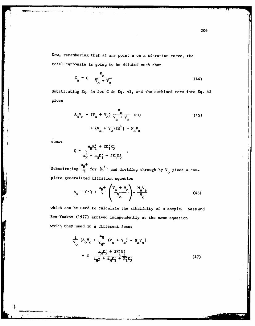
206

Now, remembering that at any point n on a titration curve, the

total carbonate is going to be diluted such that

VC =C 0 (44)

a o

Substituting Eq. 44 for C in Eq. 41, and the combined term into Eq. 43

gives

VAoV - (V + Vo) C-Q (45)0 0 a o V+ Va 0

+ (V + V) H = NaV

where aa

Q= 212a H + alKI. + 2KIK2,

all+Substituting : for [le ] and dividing through by V gives a com-

plee gnerlizd ttraionequation

ae + V O + ° NVA°0 C'Q + -y _ = (46)0 0which can be used to calculate the alkalinity of a sample. Sass and

Ben-Yaakov (1977) arrived independently at the same equation

which they used in a different form:

[A V + -!L (V + V) - NaVV0 00 YH+ a a

a.Kj + 2K'K'"C 12 (47)

a2+ a HKI + KK

207

They have used a two step process to solve Eq. 47 for A0 , C, K'O1'

K, and y,+. The first step involves setting the right hand side

equal to zero, and then solving the left hand side for A and yH+

00by linear regression. A° and H+ are then used as constants to

solve all of Eq. 47 using a series of guesses for K' and linear

regressions techniques to determine the best fit values of K', K'

and C. Their solution technique was applied to the Orca Basin brine

titrations. The mathematics of their solution are outlined for

completeness in Table 20.

NaHCO Titration

3

Additional knowledge of the carbonate system can also be

gained by addition of one individual component to a solution and

examining the resultant perturbations. The parameters that can

easily be monitored are carbonate alkalinity, total CO2 and pH.

The interdependence of carbonate alkalinity, total CO2 and pH is

described by a Deffeyes (1965) diagram showing the variations of

alkalinity with input of carbon dioxide at various pH values.

Fig. 40 gives an example of a typical Deffeyes diagram for normal

salinity sea water. The pH is uniquely determined for each value

of total CO2 and alkalinity. Also shown on this figure are the

relative changes in carbonate alkalinity and total CO2 due to the

addition of bases or acids, carbon dioxide, bicarbonate, ions,

carbonate ions or distilled water. By adding NaHCO 3 to a solution,

both the alkalinity and the total inorganic carbon are increased

208

Table 20. Sass and Ben-Yaakov (1977) mathematical solution to thegeneral titration formula. Primes on constants are omitted forsimplicity.

General equation, LHS RHS

- N aV)= C (47)o yH+ oa2 + aHKI + K K2

STEP 1: At low pH, RHS is negligibly small and can be neglected,thus

a+ (Vo + Va =-AVoYH+ + NaYH+ " Va (48)

This equation has the linear form y = m + Kx, where

y a + (Vo +V) m=AV YH+

X= Va K= NAY

YH+ and A can be determined by linear regression since aH+ and

(V + Va) change for each titration step.

STEP 2: Define Z as the LHS of the general equation andrearrange

2Ky+ a.= CKI - K1 Z (2K2 + aH + ) (49)2K2+ aH+2K 2 + a I.

Using A and YH+ from Step 1, Z becomes a known quantity. Byguessing K2, Eq. 49 has a linear form with

Z(a'H+)2y 2K2 +aH+ mCK1

K2 + all+x= Z%- K =-K 1

2 2 + a,+

Using linear regression techniques, C, K1 and r2 (coefficient of

determination) are determined for each guess of K2 . By iterationtechniques, successive values of K2 are used until the r2 valueclosest to 1.0 is obtained. The calculated Kl and C at that valueof K2 thus provide the best fit of the titration points to themodel.

IL

209

~110

E 4))

< 0

- ---------- 5.0 14.0-

-0.51i0 2

TOTAL C02 (mmol-liter -l)

i /- /oHCO NOCOT

/"2

- UTIONVCA

Fig. 40. Typical Deffeyes diagram for sea water(after Deffeyes 1965).

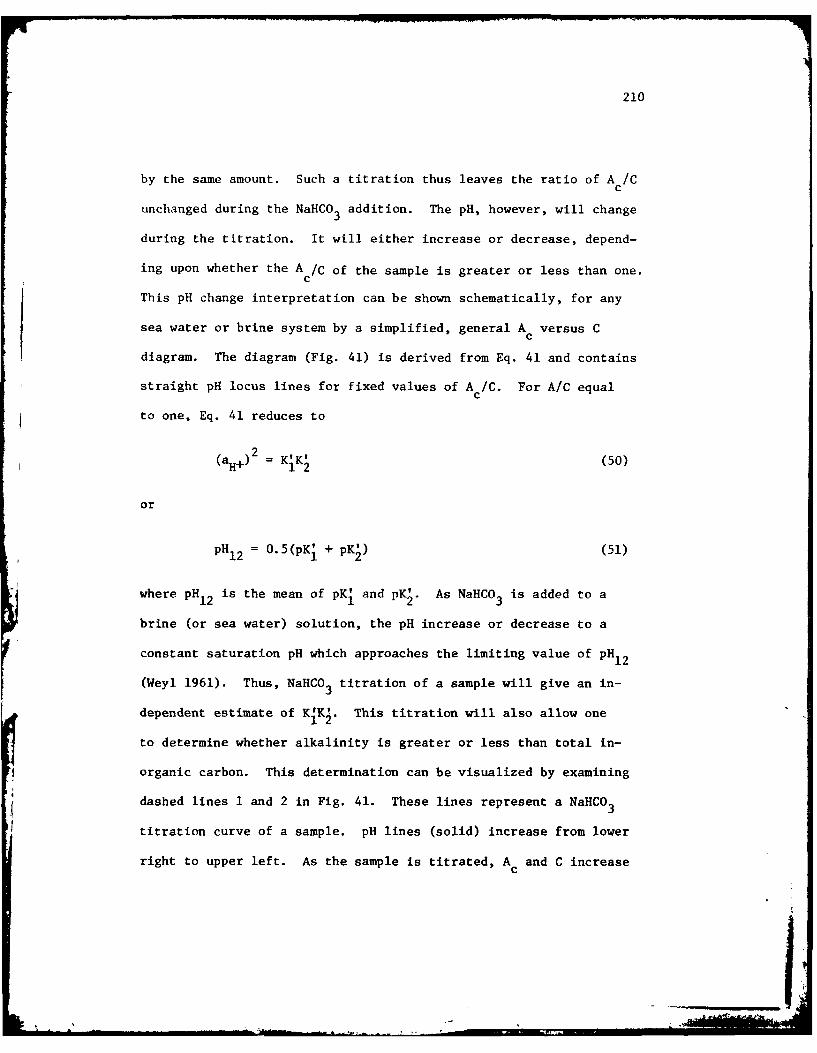
210

by the same amount. Such a titration thus leaves the ratio of A /CC

unchanged during the NaHCO3 addition. The pH, however, will change

during the titration. It will either increase or decrease, depend-

ing upon whether the A /C of the sample is greater or less than one.c

This pH change interpretation can be shown schematically, for any

sea water or brine system by a simplified, general A versus Cc

diagram. The diagram (Fig. 41) is derived from Eq. 41 and contains

straight pH locus lines for fixed values of A /C. For A/C equalc

to one, Eq. 41 reduces to

2 , ,( =+) = KIK2 (50)

or

pH 2 = 0.5(pK' + pK) (51)

where pH1 2 is the mean of pK and pK2. As NaHCO3 is added to a

brine (or sea water) solution, the pH increase or decrease to a

constant saturation pH which approaches the limiting value of pH1 2

(Weyl 1961). Thus, NaHCO3 titration of a sample will give an in-

dependent estimate of KIK 2' This titration will also allow one1 2~

to determine whether alkalinity is greater or less than total in-

organic carbon. This determination can be visualized by examining

dashed lines I and 2 in Fig. 41. These lines represent a NaHCO3

titration curve of a sample. pH lines (solid) increase from lower

right to upper left. As the sample is titrated, A and C increasec

211

A<.C

or A A<C >C)

212

at the same rate. If A = C, no pH change is observed. For A<C

(line 1), pH increases and if A>C (line 2), pH decreases during the

titration, at least up to bicarbonate saturation. Thus, a NaHCO3

titration of a sample yields independent information as to whether

the alkalinity of a sample is greater than or less than the total

CO2.

Buffer Intensity

The buffer intensity or buffer capacity, B, of a solution is

the amount of acid or base required to change the pli by one unit.

Since Eq. 41 represents the carbonate alkalinity-total CO2-PH re-

lationship of a solution, it is the starting point for determining

the buffer intensity. By taking the derivative of Eq. 41 w'th

respect to aH+, one arrives at an expression for the buffer in-

tensity of a solution (Pytkowicz and Atlas 1975)2

a H + 4K'a + KIK'B = 2.303 C K! a -H 2 H 12 2(52)

(aH + KIaH + KIK2)H 1 2

The plus signs on the hydrogen activity are omitted here for

simplicity. Thus for two systems, the buffer intensity (capacity)

of each system can be compared for any pH values, if the total

CO2 and equilibrium constants are known.

2.

213

Results and Discussion

pH and Total C02 Relationships

In the aerobic Gulf of Mexico waters, in the region of the

Orca Basin, profiles of pH and total carbon dioxide (Fig. 42) are

typical of the oceanic environment. Surface pH is about 8.2 +- 0.1

and decreases with depth to slightly less than 7.8 at 500 meters,

before increasing to 7.9 in the deeper water. The total CO 2depth

profile is almost a mirror image of the pH distribution. Total

CO 2 increases with depth are a major cause of the decreasing pH.

These increases in Gulf CO 2levels result from the aerobic res-

piration of marine organisms (see Table 12), which causes an

oxygen minimum where total CO 2 is highest and pH1 is lowest.

Below 2100 m in the Orca Basin, the total CO 2agiinrae

and pH decreases as oxygen levels begin to decrease. Fig. 43

shows the p11 and total CO. profiles through the Orca Basin inter-

face into the brine. pH decreases to 6.83 in the high salinity

brine, while total CO 2increases to an average of about 4.45 mmol.

liter- . Sackett et al. (1979) have shown that the excess CO 2in

the brine (relative to deep Gulf values) results from introduction

of isotopically light, biogenic CO 2into the Orca Basin water.

The pH decrease reflects this increase in C02,' but the change in

pH may also be affected by the total ion composition of the brine.

This possibility will be discussed in the next section.

214

pH7.7 7.8 7.9 8.0 8.1 8.2 8.3I is 1I

0 0000 00 p

oo U

o0 oU

,Oo0 Z C02 I

So U

E 00 0o

SGULF Of MVE,(ICO"-F- 77-G--3

Il STA 2-3Q

o U

1500-

0 o2000-

II I I

2.2 2.3 2.4 2.5TOTAL C02 (mmol liter")

Fig. 42. pH and total carbon dioxide depth distribution inthe northwestern Gulf of Mexico.

-.. L.

215

pH6 7 8 9

2000

In ORCA BASIN

2100 -77-G-3

p

- r 77-G-13

) E

2200

w -00

2300 - C'

IIpH C02

0112400 -

I I

2 3 4 5TOTAL C02 (mmolliter "')

Fig. 43. pH and total carbon dioxide profiles through theOrca Basin brine interface and into the high salinity brine.

216

In the interface region, there is an obvious discontinuity in

both the pH and total CO 2 depth distribution. Both parameters

follow a predictable pattern (based on 0 2consumption and CO 2

production) down to about 2210 m, then change sharply, before con-

tinuing their expected increase (C02 ) or decrease (pH) into the

high salinity brine (see Fig. 43). The total CO 2 profile shows

only a one point maximum on cruise 77-G-3, but the inverse rela-

tionship with pH contributes to the reliability of this data point.

Sackett et al. (1979) also observed the same discontinuity in their

total CO 2 data at this level. However, they chose to ignore the

single point maximum and they drew a smooth curve through the other

data points in this region. Data from cruise 77-G-13 is more

detailed in this zone (open squares in Fig. 43). These data con-

firm the CO 2discontinuity that was observed along with pH and

oxygen anomalies in this zone.

A detailed plot of pH and oxygen with depth through the inter-

face region is shown in Fig. 44. Data from two different years

are plotted for pH. It is apparent that the discontinuity in the

pH-depth profile occurs in transition zone T3, the zone where

salinity increases from 50-7O*f.. and oxygen concentration is low,

but present. Thus, the unusual oxygen step-region has a charac-

teristic pH profile change associated with it, along with the

large temperature gradient shown in Fig. 10. The decreasing pH

down to 2210 m reflects increasing production of CO 2 through the

... . .-

217

pH6.5 7.0 7.5 8.0

2100

2200 - - _02-

S

E: 2300 -

Iq

3: ORCA BASINI-tt & 77-G-3

LLI 0 78-G-2

2 500

I I pHII

0 50 100 150

OXYGEN(pmoI.Iiter)Fig. 44. Detailed plot of pH and dissolved oxygen through

the interface region of the Orca Basin.

I I ! _______________ I II

218

increasing density region. The 6 13CO 2 data of Sackett et al. (1979)

support this concept, with Increasingly lighter (isotopically) CO 2

found as the interf ace is traversed.

The increase in pH and decrease in total CO 2through the oxygen

step region (transition zone T3) are not completely understood. The

factors acting to cause this discontinuity must be a complex of mixing

and biological processes. Both temperature and salinity change

rapidly in this region. Physical mixing processes may be important,

but significant transport of carbon dioxide from the brine is ques-

tionable, since transport through the interface probably occurs only

by molecular diffusion. Another, probably more significant process

would be degradation of organic material at the top of this low

oxygen region. Particles settling on to the interface would undergo

decay, mediated by microbial populations which are as high as this

interface (LaRock et al. 1979) as at some sediment-sea water inter-

faces (Zobell 1942). Degradation of organic matter would produce

more CO2 where the bacteria biomass was highest, at the top of this

zone. Decreasing pH would result from this CO increase. The pH2

increase might also be affected by ammonia production there, or by

some slight diffusion of ammonia Into this region from the brine

below. Addition of Ammonia to the water would cause the pH to

increase. However, the magnitude of this effect is unknown. A

detailed survey of physical and biological parameters in this low

oxygen zone is needed to explain the pH and CO 2 distributions.

In the high salinity brine, there are no obvious trends in

either pH or total CO2 , Sackett et al. (1979) also found

219

relatively constant values for all other carbon budget components

in the high salinity brine. They reported a 61 3C of the inorganic

carbon of -6.4 + 1.0/ oo. This negative 6 13C value is indicative

of biogenic input of carbon dioxide into the brine. They esti-

mated that the biogenic CO2 input must have a 613C of -330/. to

produce the net 613C value observed. Average total CO2, pH and

613CO2 values for several brines are compared in Table 21. With

no change in the dissociation constants, Eq. 41 predicts that pH

will decrease as total CO2 increases. This is indeed the case for

the Orca Basin. There is a two-fold increase in CO2 levels due to

CO2 production in the brine. However, with the highest total CO2

of all the brines listed in Table 21, the Orca Basin brine also

has the highest pH. All three brines have evidence of biogenic

CO2 input, based on the 613C data. The higher Orca Basin pH must

result from the Orca Basin brine having a higher buffer capacity

than either the Dead Sea or Red Sea brines.

If one assumes that the origin of the excess CO2 is biogenic,

then the major concern becomes the species distribution and effect

of this excess CO2 in the brine. Kennett and Penrose (1978) have

noted that the calcite microfossils in the Orca Basin sediments

are well preserved. This effect must result from a change in the

carbonate system distribution in the brine. Other (non-brine)

Gulf sediments with high CO2 levels show no exceptional calcium

carbonate preservation. The following sections describe the

220

Table 21. Total carbon dioxide, 613C-C0 2 and pH from severalbrine areas.

Total CO2 613CPBrine (mmol'liter- ) (/.o)

Orca Basin 4.57 -16.4 6.83

t *Red Sea

Discovery Deep 0.60 -16.8 6.5

Atlantis II Deep 2.80 -5.6 5.61

Dead Sea 2.55 - 6.3

* Data from Weiss (1969).

t Data from Sass and Ben-Yaakov (1977).

! .~

4-..., _ __. -a~ ~ - - -i

221

experimental data used explain why the pteropod shells are well

preserved in the Orca Basin.

Brine Dilution Experiment

The results of the pH-dilution experiment for the Orca brine

and Gulf of Mexico sea water are shown in Fig. 45. Four dilution

experiments were undertaken, two with brine and two with Gulf of

Mexico sea water. In all of the dilutions, the pH increased

initially and then decreased after going through a maximum. Amit

and Bentor (1971) described this type of pH response with dilution

as being due to the "hidden alkalinity" effect. Sass and Ben-

Yaakov (1977) noted however, that this response is actually due to

the change in the ionic strength of the solution, which in turn

causes an increase in the dissociation constants of the carbonate

system, thus removing hydrogen ions from solution.

Upon dilution with distilled water, the pH of both Orca Basin

brine samples increased progressively. The two brines were pre-

pared differently before the experiment. One sample was stirred

for 24 hours before the dilution was begun, while the other was

fresh, preserved brine right out of the bottle. The effect of the

stirring was to reduce the total carbon dioxide of the brine down

from 4.41 mmol-liter to 3.44 mmol liter . The brine with the

higher total carbonate (closed diamonds in Fig. 45) has an initial

pH of about 7.3 and increases only to a pH of about 7.8 at a

_ _ _ _ _ _ _ _ _ _ _ _ _'.--. °- -I " I I

222

p H( 8.68.4

8.2

8.0

7.6 A

7.4 dlI

7.2

7.0-v Orca Basin brine (stirred)

6.8- a Gulf of Mexico surface waterA Gulf of Mexico deep water

6.6 -A Orca Basin brine

300200 100 50 30 20 10 4 2

Salinity (o/oo)

Fig. 45. pH versus log salinity dilution curves for twosamples of Orca Basin brine and for surface and deep waterfrom the Gulf of Mexico.

223

salinity of 35 0/00. The carbonate depleted brine (initial pH = 7.8)

reached a pH of 8.5 at 35 0/ salinity. The differences between

the two brine dilution curves are a direct result of one sample

having more carbon dioxide.

Fig. 46 shows that relatively little, if any, carbon dioxide

was lost during the dilution experiment. The carbon dioxide in

the two experiments both show a regular dilution curve, with only

the slopes different, due to different initial amounts of carbon

dioxide in the brines. Yet the initial carbon dioxide difference

makes all the difference in the pH-dilution curves. The brine with

the higher total CO2 never approximates the pH of the Gulf sea

water. The brine with the lower CO2 constant has the upper part of

its dilution curve in the sea water pH range. The Dead Sea dilution

curves of Amit and Bentor (1971), presented in Fig. 38, show a

relationship similar to the low CO2 curve for the Orca Basin.

The importance of biogenic carbon dioxide to the carbonate

system in the Orca Basin is obvious from the pH-dilution results.

In the Dead Sea, the surrounding area is fairly desolate and little

organic carbon enters the Dead Sea brine. With the absence

of biogenic carbon dioxide in the Dead Sea, the total carbonate

-Imeasures only 2.5 mmol-kg , a value close to the levels found in

the nearby Elat Sea water (Amit and Bentor 1971). Thus when the

Dead Sea brine is diluted down to sea water salinities, the car-

bonate content is much reduced, and the pH of the diluted brine

224

.- (CA BRINE .o4.41

4.0 0LUTION EE -

3.0- FRESH BRINE 3.44q0 X .

Q 7

Z 2.0 70

0 ' " BRINE STIRRED0 ! 24 hrs

0 -- i _ _ - i , _L . .0-

0 50 100 150 200 250 300-A LINITY (16)

Fig. 46. Change in total carbon dioxide with dilution ofOrca Basin brine. These CO2 measurements were made on the samesamples analyzed for pH and shown in Fig. 45. Total CO valuesfor each brine sample are shown in units of mmol-liter-f.

225

exceeds the pH of the Elat Sea water. In the Orca Basin with the

high total carbonate, the dilution pH values are lower than the sea

water pH values. This effect must result from the higher total

CO2 of the Orca brine, as well as the fact that the salt did not

originate from present Gulf of Mexico sea water.

The pH-dilution curve of the Orca brine is also shifted to

the left, compared to the dilution curve for the Gulf of Mexico

water. This effect was not observed by Amit and Bentor (1971) who

compared the Dead Sea brines to the Elat and Mediterranean Sea

waters. This shift means that a higher pH was reached at a higher

salinity in the Orca brine, as compared to the Dead Sea brine.

This response may be due to the difference in ionic nature of the

two brines (see Table 3). The Dead Sea brine is higher in calcium

and magnesium and relatively depleted in sulfate. In contrast to

the Orca Basin, and in contrast to almost all other known surface

water bodies (Nissembaum 1975), magnesium is the dominant cation

in the Dead Sea brine.

The pH-dilution curve is controlled predominately by a

relaxation of the dissociation constants as more water is added

to the brine. The two brines would be expected to respond differ-

ently if changes in the dissociation constants were due to the

different ionic compositions of the brines. Ben-Yaakov and Gold-

haber (1973) noted that sea water dissociation constants of the

carbonate system vary in sensitivity to changes in different ions.

226

They defined a sensitivity parameter for the change in each con-

stant with respect to the major Ions. They showed that the

apparent constants are especially sensitive to a variation in the

concentration of magnesium in solution. Ionic composition, as well

as the total ionic concentration, are important in determining the

carbonate system dissociation constants. The differences in the

ionic balances between the Dead Sea and Orca Basin can be dramnati-

cally seen when referenced to the chloride content of each brine.

Relative to chloride, and compared with average Gulf of Mexico sea

water, Mg and Ca are enriched by a factor of about three in the

Dead Sea, but they are depleted by a factor of one-third and one-

tenth, respectively, in the Orca Basin (Table 22). Ion complexa-

tions due to the higher magnesium and calcium levels in the Dead

Sea brine would thus allow the pH levels to increase more slowly

with dilution, than in the Orca Basin brine where the concentra-

tions of those important ions is lower.

Alkalinity Versus Total CO 2

As was discussed earlier, titration of a bicarbonate solution

with one of the carbonate system components can yield useful

information as to the species distribution, when the data is in-

terpreted on a Deffeyes diagram. The results of a titration of

the Orca brine with 1.0 N sodium bicarbonate solution is shown in

Fig. 47. With reference to Fig. 41, the initial increase in brine

227

Table 22. Ion enrichment factors relative to sea water forcalcium and magnesium (referenced to chloride).

Brine Ca Enrichment Mg Enrichment

Orca Basin 0.346 0.105

tRed Sea 1.436 0.078

Dead Sea t 3.716 2.828

* Shokes et al. (1977).

Brewer et al. (1969).

Amit and Bentor (1971).

4 ..-,".-,,'

228

9

8 ,ORCA BASIN BRINE

pH7

DEAD SEA BRINE

5 0 6

Vol. NaHCO 3 (ml)

Fig. 47. Change in pH of the Orca Basin brine and Dead Sea brineswith addition of 0.5 N NaHCO3 . Solid symbols are pure brine and open

symbols are 50% dilutions (Dead Sea brine data from Sass and Ben-Yaakov 1977).

229

pH with the addition of the NaHCO indicates that the total car-3

bonate level in the Orca Basin is higher than the alkalinity. The

Dead Sea data of Sass and Ben-Yaakov (1977) are shown for comparison.

In the Dead Sea brine, the alkalinity was greater than the total

carbon dioxide, as seen by the reduction of pH with the addition

of bicarbonate (see Fig. 47).

It should be pointed out here, that the brine that was used

for titration with sodium bicarbonate was stored (with sodium azide

poisoning) for several months before titration. It is possible

that there was some change in the carbonate composition before

titration. I make this comment since Millero et al. (1979) have

reported that the total alkalinity of the brine is 4.015 + 0.008

meq'kg- I for Orca Basin brine. This value translates to 4.75

meq.liter- I using a value of 1.185 for the density of the brine at

room temperature. This alkalinity value is greater than the 4.57

mmol.liter- I total inorganic carbon value reported by Sackett et

al. (1979) and also higher than the 4.50 mmol-liter- I determined

in this study. It is possible that the ammonia in the water is

causing the higher alkalinity that was measured by Millero et al.

(1979). Thus the influence of other factors may affect the

alkalinity in the Orca Basin, as they do for other anoxic hyper-

saline waters (Gaines and Pilson 1972).

To confirm the conclusion that A/C was less than unity,

several brine samples were left open to the air and stirred for 24

230

hr to remove CO2 . Titration of these samples with 0.5 N NaHCO 3

produced a titration curve in which the pH decreased with addition

of titrant. The lower CO2 sample had an alkalinity greater than

the total CO2 concentration. This titration also showed that the

observed pH changes were not due to the brine dilution, since dilu-

tion alone, at either high or low total CO2 levels, would increase

the pH of the brine.

Ala|lnltv in the High Salinity Brine

As discuss,-d in the carbonate model section, using the calcu-

'Lm -iethods of Sass and Ben-Yaakov (1977) with an acid titration

of a :IuaLl()n allows calculation of the dissociation constants as

wf-I! a alkalinity and total carbonate. A typical titration with

HC1 .,f Orca Basin brine is depicted in Fig. 48. Also shown is an

HCI titration of deep Pacific Ocean sea water (salinity=34.8/0 ).

The following observations can be made from this titration:

(1) The pH of the inflection point of the HC titration is a

function of the salinity of the solution.

(2) The shape of the HCl titration curve for the Orca brine

is similar to the sea water curve, but shifted downward

(to lower pH) due to the high carbonate content of the

brine and the difference in dissociation constants result-

ing from the high salinity.

231

0 0

U)

C4I

eq $* w

44°

0

z , ,1

O ~~~ cOi D Oeso 0

*>

so 0 0

00 0

-J 0 00

W ) V) C 144*k C34

X ~*.~

232

(teFor interpretation of the data in Fig. 48, the buffer capacity

(teincremental change in pH for a given volume of HCl added) was

calculated and plotted for each series of data points. The results

of this calculation are presented in Fig. 49. The buffer capacity

versus pH curve is also plotted for the sea water HCl titration

as a comparison. Maxima and minima in these curves correspond to

the pK' values of the dissociation constants of the carbonate

* I system in each solution. For example, the pK' value for sea

water would correspond to the minimum at a buffer capacity of about

* 0.25. The pl(' value for sea water corresponds to the buffer capacity

maximum at a pH of about 6.1. Since the pH of the Orca Basin is

so low, there is no upper minimum to use in graphically determining

the pK'. The pK{ corresponds to the maximum in buffer capacity

which occurs at a pH of 5.5. A pIof 5.5 for the brine repre-

sents a factor of three increase in the KIdissociation constant,

compared to sea water.

Application of the iterative solution technique of Sass and

Ben-Yaakov to this titration allows more accurate calculation of

the dissociation constant. Using the titration data plotted in

Fig. 48 and the mathematical sequence given in Table 20, the al-

kalinity, the total carbon dioxide, and the carbonate dissociation

constants were calculated for the Orca Basin and f or sea water,

for comparison. The results of this calculation are presented in

Table 23. Analysis of other samples gave lover carbon dioxide

233

0Vr ( -

oO -4 4-'C

I . cc~J

w0r

to- 10

o0 w4a

I4 0

0 H r

z ).J -, 4J

U) 0 r .

0

0~ a.~CM m ) 04P.I,

"-4 '4-o

0 U- -4 c oI U 41JW

ujU vu40 ::) oo. WW

M 0U4.3W-

234

Table 23. Calculated alkalinity and carbonate dissociationconstants for seawater and Orca Basin brine.

Brine Alkalinit Total CO2 pK 1 pK 2Brine (meq-liter_- (mmol-liter-l K K

Sea water 2.20 2.13 5.80 9.14

Orca Basin brine 4.701 4.750 5.49 8.34

Dead Sea brine 3.86 4.41 5.09 6.23

From Sass and Ben-Yaakov (1977).

235

concentrations, but also lower alkelinity concentrations, indica-

tive of some CO2 loss.

The dissociation constants increase with increasing salinity

in the Orca Basin. In the Dead Sea brine, Sass and Ben-Yaakov

(1977) also noted this increase in the dissociation constants.

Their values are given in Table 23 for comparison. It is immedi-

ately obvious that the dissociation constants of the Dead Sea

brine are altered more (relatively to sea water) due to the in-

creasing salt content, than are the constants for the Orca Basin.

This magnitude of difference can be seen more dramatically

when the distribution of carbonate system species is calculated

for the Orca Basin and the Dead Sea brines. The results of the

species distributions as a function of pH are given in Fig. 50.

The results are presented as relative percentages of each species

as a function of pH. Presented in this manner, the relative dis-

tributions in each solution can be directly compared without

considering the total carbonate concentration.

The distribution of the carbonate species in the Dead Sea

brine is very different from either sea water or Orca Basin brine.

At the natural pH of the Dead Sea, the concentrations of carbonate

and bicarbonate ions are approximately equal. This is atypical for

the other systems, where bicarbonate is by far the dominant in-

organic carbon ion in solution at in situ pH values.

The shape of the distribution in the Orca Basin is very much

like that of sea water, but all distribution curves are shifted

236

100H2 CO 3 ,- HC 3

80 3,

60-1t . I \

40SES SEA

WATER20 I

C~0

60 . / I

.1.I o

LU40 S

0. \

\ ORCA

20 /

20 BASIN

0-

80-..

60 -

". / I

40 '

/ DEAD

20 SEA

0 14 5 6 7 8 0 10 11

pH

Fig. 50. Carbonate system species dis-

tributions f or sea vater, the Orca Basinbrine and the Dead Sea brines. The vertical

dashed lines indicate the pH ranges of thenatural systems.

*"-

237

toward lower pH values. Orca Basin brine has a pH of 6.83. This

small difference in the species profiles underscores the chemical

nature of the Orca Basin brine. The Orca Basin brine is like sea

water that has been saturated with sodium chloride. On the other

hand, the major ionic ditfer'nces between the Dead Sea brine and

sea water play havoc with the carbonate species distribution there.

Sass and Ben-Yaakov (1977) have attributed most of the disparity

in the Dead SeL, carbonate system to the concentration of magnesium

in the Dead Sea brine. The bicarbonate to carbonate dissociation

constant is about threefold more sensitive to variations in mag-

nesium concentration than is the K' (Ben-Yaakov and Goldhaber

1977). This effect is attributed to the relatively high stability

of MgCO0 complex as compared to that of MgHCO3 (Garrels and

Thompson 1962). The high K' dissociation constant for the Dead2

Sea brine causes the observed distributions. Since both K' and

K' are greater, but only two or three times sea water values, the2

Orca Basin brine distributions are similar to sea water.

Pteropod Preservation in the Sediments

The consequences of salinity causing an increase in the

dissociation constants, combined with the biogenic total CO2 in

the brine has resulted in such a high concentration of carbonate

ion in the sediments, that there is rather striking preservation

238

of carbonaceous material in the Orca Basin sediments. Even ptero-

pod tests, which are made of the more soluble aragonite, are

preserved in the sediment. Fig. 51 shows several electron micro-

scope photographs (taken by L. A. Barnard) of some of the ptero-

pods found in the Orca Basin sediments. As noted by Kennett and

Penrose (1978), the preservation is striking. There is no

evidence of even the tiny etch marks often observed on

calcium carbonate tests undergoing slow dissolution in typical

marine sediments (Alexandersson 1975). Fig. 52 shows one of the

pteropods found in the basin, and two additional magnifications

of one portion of the pteropod. These micrographs show that there

is absolutely no dissolution of this soluble aragonitic species

(Cavolinia longirostris).

The observation of the well-preserved microfossils in the

sediment, with no evidence of CaCO3 precipitation, implies

the Orca Basin sediments are in equilibrium with respect to cal-

cium carbonate. Since the concentration of carbonate ion in the

brine is no higher than in normal sea water, one must consider

the solubility coefficient of calcium carbonate in the brine sedi-

ments to be different than in normal marine environments. Also

-ithere is an excess of 17 mmol-Ca.kg brine in the Orca Basin.

This excess calcium would contribute to the preservation of the

calcite and aragonite tests in the brine. But, where did this

excess calcium come from? Could it be from past dissolution of

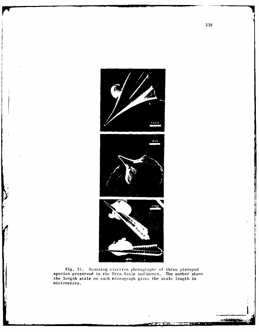
239

4f

Fig. 51. Scanning electron photographls of three pteropodspecies preserved in the Orca Basin sediments. The number abovethe length scale on each micrograph gives the scale length inmicrometers.

_ _ _ ,.,

'Fig, 52. Three scanning electron ph'.tographs of a C;ivolii'Ja

longirostLki. pteropo3 found in thfe Orca EasirL sedim,,ents. The rviiml,,wr

above eachi length scale on each micrograph gives the ;calP length inl

micrometers. Even it highi magnificati~on, there is no evideflcc of

aragonite dissolution in the Orca Basin sediments.

241

calcium carbonate in the brine? This seems improbable since the

pteropods in the brine are preserved throughout the sediment

column (Addy and Behrens 1980). In one core section at a depth of

689 cm, Addy and Behrens (1980) found that the percentage of sand

increased significantly, to 21%. The increase in sand was entirely

skeletal, calcium carbonate tests. In fact, they noted that

the preservation of calcium carbonate in the sediments increased

the sedimentation rate by as much as 21 cm-ka -. Thus, the excess

calcium must have an alternate source.

Excess Calcium and K ' of Brinesp

It will be shown here that this excess calcium originated

with the inflowing brine and not from calcium carbonate dissolu-

tion in the basin. CaCO3 can decompose to form

CaCO-- Ca+++ CO (53)3 3

With this dissolution, Ca++ increases (1 mole) along with alka-

linity (2 equivalents) and total CO2 (1 mole). At the same time,

organic material is decomposing in the brine producing C02, HNO3

(or NH3) and H3PO4 (Table 12). In sea water CO2, HNO 3 and H3PO4

react with CO (Brewer et al. 1975). Thus, the combined decom-

position equation (aerobic) which includes CO reaction can be

written as

242

(CH20)I0 6 (N 3)I6H3P04 + 13802 + 124C0; (54)

= 16NO + HPO + 230 HCO- + 16H 03 4 3 2

This combined reaction scheme (Eq. 54) results in an increase of

106 moles in ECO2 and a decrease in 17 equivalents in alkalinity.

Chen (1978) has discussed this combined effect of CaCO3 dissolution

and decomposition of organic matter in the ocean. He represents

the decomposing of x Umol of CaCO 3 and y pmol of organic matter in

sea water by the expressions:

ATA = 2x - 17y (55)

AC02 =x + 106y (56)

ANO3 = 16y (57)

where TA is in micruequivalents and ZCO 2 and NO3 are in micromoles.

The same equations are applicable to anaerobic decomposition since

the same ratios are involved, only NH3 is produced as the terminal

nitrogen product. In examining the Orca Basin, Eq. 57 becomes

ANO3 + ANH3 = 16y (58)

since both aerobic (initially) and anaerobic processes have been

active in bringing the brine to its present state. Eqs. (55) and

(56) and Eqs. (56) and (57) were solved by Chen (1978) for x, the

CO3 concentration which is equivalent to ACa, the change in

243

calcium concentration (see Eq. 54). The results are

ACa = x = 0.46288 ATA + 0.074236 AECO3 (59)

ACa = x = 0.5 ATA + 0.53125 ANO 3 (60)

Since alkalinity, total CO2 , nitrate and ammonia have all been

measured for the Orca Basin, the predicted ACa+ + can be calculated

showing the increase in Ca+ + from possible dissolution of CaCO3

and decomposition of organic matter. These calculations are

shown in Table 24. Eq. 59 predicts a ACa+ of a 0.96 mmol-kg-

while Eq. 60 predicts 1.12 mol'kg- I for an average of 1.04 mmol-

kg . This increase is far below the measured ACa (compared to

deep Gulf water) of 17.0 mmol-kg- I (Table 3). It can also be

calculated (Table 24) that if enough Ca+ + were put into Gulf

sea water to reach the Orca Basin levels, the resultant alkalinity

would be approximately 35 meq-kg . Thus the excess Ca in the Orca

Basin must have entered with the original brine, probably from the

dissolution of calcium sulfate along with NaCI.

The complete preservation of the aragonitic pteropod shells in

the Orca Basin is unusual. While some other anoxic environments have

partial preservation of pteropod tests (see, for example, Berger

and Soutar 1970), preservation is complete in the Orca Basin

sediments. Since no CaCO 3 precipitation occurs in the Orca Basin,

one can assume that Orca brine is in equilibrium with respect

244

Table 24. Calculations showing the possible changes in totalcalcium content resulting from the increases in alkalinity, totalCO2 , and ammonia in the Orca Basin.

Date for Calculations-ACa+ + = 17.0 mmol-kg-1 (Shokes et al. 1977)

ATA = 4.015 meq-kg-1 (Millero et al. 1979 and this study)

AECO2 = 1.913 mmol-kg- 1 (Sackett et al. 1979 and this study)

ANO + NH3 = 441 umol'kg (this study)

Basic Equations

a. ACa+ + -0.46288 ATA + 0.074236 AECO2

b. ACa = 0.5 ATA + 0.53125 (ANO3 + NH 3)

Ca+ Predicted Changes

+4. -1a. ACa = 0.46288 (1765 weq'kg ) + 0.074236 (1.913 pmol-kg)

ACa+ + = 958 umol-kg

b. ACa+ + = 0.5(1765 ieqkg- ) + 0.53125(441 rmolkg- I)

iACa+ = 1117 Pmol'kg 1

Average = 1037 pmol-kg1

Alkalinity Required to Produce Orca ATA

Ca+ + - 0.074236 CO2a. ATA = 0.46288

ATA - 36.4 peq.kg- 1

Ca 4 + - 0.53125 (NO- + NH3 )b. ATA 0.5 3 3

ATA - 34.5 peq.kg- 1

Average TA 35.5 peq-kg- I

245.

to aragonite, and the apparent solubility product (K'p) for

aragonite can be calculated. This constant is defined in terms

of total concentration, i.e. the product of the total calcium

(Ca+ +) and total carbonate (CO;) ions. Total calcium is given in

Table 3. Carbonate ion concentration is obtained from the

relationship:

[CO=] A C K2K (61)

C3] (ae~t + 2KI)

Using the pH of the brine as 6.83 and a pK' of 8.34, one obtains

a value of 3.2 x 10- 6 mol 2.kg- 2 for K ' at 25*C. This valuesp

is about six times larger than the corresponding value for sea

water (Ben-Yaakov ind Goldhaber 1973). If the Orca brine had normal

sea water calcium concentration (see Table 3), the ion product for

[Ca++][CO;J would be 1.2 x 10 - 6 mol 2.kg- 2 . This would make the

brine undersaturated with respect to aragonite by a factor of

three. Thus, it is the high calcium content of the brine which

causes the complete preservation of the aragonitic pteropod shells

in the Orca Basin sediments.

246

CHAPTER VI

SUMMARY AND CONCLUSIONS

The advective, diffusive, and reactive processes acting upon

the dissolved gases in the hypersaline waters of the Orca Basin

are no different than in other marine, anoxic environments. Only

the magnitude of the constants and the rates of reaction are

affected by the increased concentrations of dissolved salts in

the Orca Basin water. The processes differ from other less saline

areas only in degree of interaction. This study has shown the

potential of dissolved gas studies in understanding those

processes.

This investigation confirmed that the Orca Basin brine is the

result of the low temperature dissolution of a sea floor salt

deposit by Gulf of Mexico sea water, with the resultant brine

flowing into the depths of the basin. The similarity of the

nitrogen to argon ratio in the Orca Basin water (exclusive of salt),

to that of deep Gulf of Mexico water (also corrected for the salt

content) supports the hypothesis of low temperature solution of a

sill salt. This first postulate was based on the ion content of

the brine, relative to evaporite and solution deposit systems.

The dissolved nitrogen and argon data provided an independent

confirmation of that mechanism of brine formation, and furthermore,

gave a temperature maximum for the dilution water of less than 5°C.

The bottom water temperature in the Gulf of Mexico is 4.2°C.

247

The step-like feature in the oxygen concentration was perhaps

the most interesting of the observations involving dissolved gases.

A simple consideration of the possible mixing processes which

occur at the brine-sea water interface revealed that it would be

possible to account for this step-like feature from mixing pro-

cesses alone. More work is needed to prove this conclusively.

Detailed, continuous, simultaneous measurements of temperature,

salinity, dissolved oxygen, and pH1 across the brine-sea water

transition regions should be made with great precision in order to

indicate accurately the nature of the mixing processes at the Orca

Basin interface.

Measurements of other parameters indicated that the brine-

sea water interface in the Orca Basin is physically active,

chemically reactive, and behaves much like the sediment-sea water

interface in other anoxic regions. This fact was most apparent

from the dissolved molecular nitrogen and ammonia distributions in

the interface and transition zones. The observed distributions

of dissolved molecular nitrogen in the low oxygen region were

strikingly similar to the near surface sediment distributions that

were reported by Barnes et al. (1975) for the southern California

borderland basin sediments. This similarity illustrates the

important laboratory potential of the Orca Basin system. The

interface there is like a sediment-sea water interface, except that

it can be sampled over a length scale of meters, rather than the

I 248centimeters and millimeters required for sediment work. In

reviewing the other constituents, such as nitrous oxide and

ammonia, these parameters also change, going from the Gulf water

into the brine, in the same manner that sea water-sediment inter-

Ltial water transitions are made in many environments. Thus, the

Orca Basin interface region could be useful in examining theI transition processes of consumption and production by which con-

centration gradients change rapidly across interface boundaries.

The dissolved reduced gases in the high salinity brine are

produced by the same decomposition processes that are operative

in other anoxic basins. The high concentrations of methane and

ethane in the brine result from the great stability of the brine

in the basin, which has a residence time of over 6000 years. Both

methane and ethane are produced in the basin. However, in spite

of the high concentrations observed, empirical evidence from

isotopic composition of the carbon compounds (methane and carbon

dioxide), along with the unusual depth distributions of iron and

hydrogen sulfide (when compared with other anoxic areas),

indicated that the rates of microbial decomposition are slower in

the Orca Basin. The presence of preserved Sargassum seaweed deep

in the sediments is further evidence for reduced decomposition

rates in the Orca Basin. Reduced microbial activity produces

little free sulfide to react with the iron in the brine. High

concentrations of iron have accumulated in the water column.

249

The carbonate system in the high salinity brine is similar

to sea water which has simply been saturated with sodium chloride.

The relative distributions of the carbonate species are the same

as those found in normal salinity sea water. The low pH in the

brine results from the input of 2.2 mmol.liter- of biogenic

carbon dioxide. The carbonate dissociation constants differ only

because of the different degree of interaction caused by the

higher salt content. The apparent solubility product constant of

aragonite in the brine is about six times larger than the corres-

ponding value for sea water at 25*C. Thus it must be the high

concentrations of calcium in the brine which has caused the pres-

ervation of pteropod shells in the basin sediments.

This investigation has shown the utility of dissolved gas

in examining the active physical and biological processes in

unusual environments. Such an examination should also answer

questions about the Orca Basin that had been posed during previous

studies. An examination of both reactive and unreactive gases

has yielded significant information about the formation of the

brine, as well as about the rates of reaction in the brine. The

objectives of this work have been met with solutions that are

internally consistent. Dissolved gases can be powerful geochemical

tracers for oceanic processes.

250

REFERENCES

Adams, D.D. 1973. A laboratory model for plankton decomposition inanaerobic and aerobic sea water. Ph.D. Thesis, DalhousieUniversity, Halifax, Nova Scotia, Canada. 228 p.

Addy, S.K. and E.W. Behrens. 1980. Time accumulation of hyper-saline anoxic brine in Orca basin (Gulf of Mexico). Mar.Geol. 37: 241-252.

Alexandersson, E.J. 1975. Etch patterns on calcareous sedimentgrains: peterographic evidence of marine dissolution of car-bonate minerals. Science 189: 47-48.

Amit, 0. and Y.K. Bentor. 1971. pH-dilution curves of salinewaters. Chem. Geol. 7: 307-313.

Antoine, J.W. and W.R. Bryant. 1969. Distribution of salt and saltstructures in the Gulf of Mexico. Amer. Assoc. Pet. Geol.Bull. 53: 2543-2550.

Armstrong, F.A.J., C.R. Stearns, and J.D.H. Strickland. 1967. Themeasurement of upwelling and subsequent biological processes bymeans of the Technicon AutoAnalyzer and associated equipment.Deep-Sea Res. 14: 381-389.

Atkinson, L.P. and F.A. Richards. 1967. The occurrence and distri-bution of methane in the marine environment. Deep-Sea Res.14: 673-684.

Atlas, E.L., S.W. Hager, L.I. Gordon, and P.K. Park. 1971. Apractical manual for use of the Technicon AutoAnalyzer in sea-water nutrient analyses; revised. Oregon State University,

Department of Oceanography, Technical Report 215. 49 p.

Barabee, J.M. and W.J. Payne. 1967. Products of denitrification by amarine bacterium as revealed by gas chromatography. Mar. Biol.1: 136-139.

Barnes, R.O., K.K. Bertine, and E.D. Goldberg. 1975. N 2 :Ar,

nitrification and denitrification in southern Californiaborderland basin sediments. Limnol. Oceanogr. 20: 962-970.

Barnes, R.O. and E.D. Goldberg. 1976. Methane production and

consumption in anoxic marine sediments. Geology 4: 297-300.

251

Benard, H. 1901. Les tourbillons cellulaires dans un nappe liquidetransportant de la chaleur par convection en regime permanent.Ann. Chim. Phys. 23: 62-144.

Ben-Yaakov, S. 1970. A method for calculating the in situ pH ofseawater. Limnol. Oceanogr. 15: 326-328.

Ben-Yaakov, S. and M.B. Goldhaber. 1973. The influence of sea water

composition on the apparent constants of the carbonate system.Deep-Sea Res. 20: 87-99.

Ben-Yaakov, S. and E. Sass. 1977. Independent estimate of pH ofDead Sea brine. Limnol. Oceanogr. 22: 374-376.

Berger, W.H. and A. Soutar. 1970. Preservation of plankton shellsin an anaerobic basin off California. Geol. Soc. Amer. Bull.81: 275-282.

Bernard, B.B. 1978. Light hydrocarbons in marine sediments. Ph.D.Thesis, Texas A&M University, College Station, Tx. 144 p.

Bernard, B.B. 1979. Methane in marine sediments. Deep-Sea Res.26A: 429-443.

Bernard, B.B., J.M. Brooks, and W.M. Sackett. 1976. Natural gasseepage in the Gulf of Mexico. Earth Planet. Sci. Lett.31: 48-54.

Berner, R.A. 1971. Principles of chemical sedimentology. McGraw-Hill Book Co., 240 p.

Berner, R.A. 1972. Sulfate reduction, pyrite formation and theoceanic sulfur budget, p. 347-361. In D. Dryssen and D.Jagner [eds.], The changing chemistry of the oceans. Alm-quist & Wiksell.

Berner, R.A. 1974. Iron sulfides in Pleistocene deep Black Seasediments and their paleo-oceanographic significance, p. 524-531. In E.T. Degens and D.A. Ross [eds.],The Black Sea -geology, chemistry and biology, Mem. 20. Amer. Assoc. Pet.Geol. George Banta Company.

Berner, R.A. 1978. Sulfate reduction and the rate of deposition ofmarine sediment-. Earth Planet. Sci. Lett. 37: 492-498.

Berner, R.A., T. Baldwin,and G.R. Holdren, Jr. 1979. Authigeniciron sulfide as paleosalinity indicators. J. Sed. Petrol.49: 1345-1350.

Borchert, H. and R.O. Muir. 1964. Salt deposits; the origin, meta-morphisis and deformation of evaporites. Van Nostrand. 338 p.

252

Bouma, A.H., L.B. Smith, B.R. Sidner, and T.R. McKee. 1975.Submarine geomorphology and sedimentation patterns of the Gyreintraslope basin, northwest Gulf of Mexico. Technical Report75-9-T, Department of Oceanography, Texas A&M University,College Station, Tx. 163 p.

Braitsch, 0. and A.G. Herrmann. 1963. Zur Geochemie des Broms inSalinaren Sedimenten, Teil I. Experimentelle Bestimmung derBr-Verteilung in verschiendenen naturlichen Salzsystemen.Geochim. Cosmochim. Acta 27: 361-391.

Breed, R.S., E.G.D. Murray, and N.R. Smith. 1957. Bergley's manual

of determative microbiology, 7th ed. The Williams and Wilkins

Co. 1094 p.

Brewer, P.G., C.D. Densmore, R. Munns, and R.J. Stanley. 1969.Hydrography of the Red Sea brines, p. 138-147. In E.T. Degensand D.A. Ross feds.], Hot brines and recent heavy metal depositsin the Red Sea. Springer-Verlag.

Brewer, P.G. and D.W. Spencer. 1974. Distribution of some traceelements in Black Sea and their flux between dissolved andparticulate phases, p. 137-143. In E.T. Degens and D.A. Ross

teds.], The Black Sea - geology, chemistry, and biology, Mem. 20.A)mer. Assoc. Pet. Geol. George Banta Company.

Brewer, P.G., G.T.F. Wong, M.P. Bacon, and D.W. Spencer. 1975.Vi oceanic calcium problem. Earth Planet. Sci. Lett. 26-81-87.

Brisou, J. and N. Vargues. 1961. Proteolysis and nitrate reductionin sea water, p. 410-414. In C.H. Oppenheimer [ed.], Symposiumon marine micribiology, Charles C. Thomas.

Broenkow, W.W. 1969. The distribution of nonconservative solutesrelated to the decomposition of organic matter in anoxic basins.Ph.D. Thesis, University of Washington, Seattle, Wash. 207 p.

Broenkow, W.W. and J.D. Cline. 1969. Colorimetric determination ofdissolved oxygen at low concentrations. Limnol. Oceanogr.14: 450-454.

Brooks, J.M., T.J. Bright, B.B. Bernard, and C.R. Schwab. 1979.Chemical aspects of a brine pool at the East Flower Garden Bank,northwestern Gulf of Mexico. Limnol. Oceanogr. 24: 735-745.

Brooks, J.M., D.F. Reid, and B.B. Bernard. 1980. Methane in theupper water column of the Gulf of Mexico. Deep-Sea Res.In press.

ILK l r e '" i n n , ,, " 1 ." -

253

Burke, Jr., R.A., J.M. Brooks, and W.M. Sackett. 1980. Light hydro-carbons in Red Sea brines and sediments. Geochim. Cosmochim.Acta (submitted).

Carlucci, A.F. and P.M. McNally. 1969. Nitrification by marinebacteria in low concentrations of substrate and oxygen. Limnol.Oceanogr. 14: 736-739.

Carpenter, J.H. 1965. The accuracy of the Winkler method fordissolved oxygen analysis. Limnol. Oceanogr. 10: 135-140.

Chen, C.A. 1978. Decomposition of calcium carbonate and organiccarbon in the deep oceans. Science 201: 735-736.

Claypool, G.E. and I.R. Kaplan. 1974. The origin and distributionof methane in marine sediments, p. 99-139. In I.R. Kaplan[ed.], Natural gases in marine sediments. Plenum Press.

Cline, J.D. 1969. Spectrophotometric determination of hydrogensulfide in natural waters. Limnol. Oceanogr. 14: 454-458.

Cline, J.D. and F.A. Richards. 1972. Oxygen deficient conditionsand nitrogen reduction in the eastern tropical North PacificOcean. Limnol. Oceanogr. 17: 885-900.

Cohen, Y. 1978. Consumption of dissolved nitrous oxide in an anoxicbasin, Saanich Inlet, British Columbia. Nature 272: 235-237.

Cohen, Y. and L.I. Gordon. 1978. Nitrous oxide in the oxygen minimumof the eastern tropical North Pacific: evidence for its con-sumption during denitrification and possible mechanisms for itsproduction. Deep-Sea Res. 25: 509-524.

Collins, A.G. 1975. Geochemistry of oilfield waters. ElsevierScientific Publishing Company. 496 p.

Cooke, R.C. 1973. The use of activated charcoal for the removalof oxygen from gas systems. Limnol. Oceanogr. 18: 150-152.

Craig, H.C. 1969. Geochemistry and origin of the Red Sea brines,p. 208-242. In E.T. Degens and D.A. Ross [eds.], Hot brinesand recent heavy metal deposits in the Red Sea. Springer-Verlag.

Crank, J. 1975. The mathematics of diffusion. 2nd edition. ClarendonPress. 414 p.

Crozier, T.E. and S. Yamamoto. 1974. Solubility of hydrogen in water,sea water, and sodium chloride solutions. J. Chem. Eng. Data19: 242-244.

254

Davis, J.B. and H.F. Yarbrough. 1966. Anaerobic oxidation of hydro-carbons by Desulfovibrio desulfuricans. Chem. Geol. 1: 137-144.

Deffeyes, K.S. 1965. Carbonate equilibria: a graphic and algebraicapproach. Limnol. Oceanogr. 10: 412-426.

Degens, F T. and D.A. Ross [eds.]. 1974. Hot brines and recentheav metal deposits in the Red Sea. Springer-Verlag. 631 p.

Deuser, W.G., E.T. Degens, and G.R. Harvey. 1973. Methane in LakeKivu: New data bearing on its origin. Science 181: 51-54.

Douglas, E. 1964. Solubilities of oxygen, argon, and nitrogen indistilled water. J. Phys. Chem. 68: 169-174.

Edmond, J.M. 1970. High precision determination of titration alka-linity and total carbon dioxide content of sea water bypotentiometric titration. Deep-Sea Res. 17: 737-750.

Edmond, J.M. 1972. The thermodynamic description of the CO2system in seawater: development and current status.Proc. Roy. Soc. Edinburgh 72: 371-387.

Emery, K.O. and D. Hogan. 1958. Gases in marine sediments. Bull.Amer. Assoc. Petrol. Geol. 42: 2174-2188.

Fanning, K.A. and M.E.Q. Pilson. 1972. A model for the anoxic zoneof the Cariaco Trench. Deep-Sea Res. 19: 347-963.

Fleming, R.H. 1940. Composition of plankton and units for reportingpopulation and production. Proc. Sixth Pac. Sci. Assoc.3: 535-540.

Fredericks, A.D. 1972. Distribution of organic carbon, p. 6-7.In Vivian C. Bushnell [ed.], Serial atlas of the marine environ-ment. Folio 22, Chemistry, primary productivity, and benthicalgae of the Gulf of Mexico. Amer. Geograph. Soc.

Froelich, P.N., G.P. Klinkhammer, M.L. Bender, N.A. Luedtke, G.R.Heath, D. Cullen, and P. Dauphin. 1979. Early oxidation oforganic matter in pelagic sediments of the eastern equatorialAtlantic: suboxic diagenesis. Geochim. Co-,mochema. Acta.43: 1075-1090.

Fuhs, G.S. 1961. Der mikrobielle Abbau von Koklenwasserstoffen.Arch. Mikrobiol. 39: 374-422.

Gaines, A.G. and M.E.Q. Pilson. 1972. Anoxic water in the Petta-quamscutt River. Limnol. Oceanogr. 17: 42-49.

255

Games, L.M., J.M. Hayes, and R.P. Gunsalus. 1978. Methane-producingbacteria: natural fractionation of the stable carbon isotopes.Geochim. Cosmochim. Acta. 42: 1295-1297.

Carrels, R.M. and M.E. Thompson. 1962. A chemical model for seawater at 25°C and one atmosphere total pressure. Amer. J.Sci. 260: 57-66.

Garrison, L.E. and R.G. Martin, Jr. 1973. Geologic structures inthe Gulf of Mexico basin. U.S. Geological Survey, Prof. Paper773. 85 p.

Gieskes, J.M. 1974. The alkalinity-total carbon dioxide systemin sea water, p. 123-151. In E.D. Goldberg [ed.], The Sea,v. 5: Marine Chemistry. Wiley Interscience.

Gille, J. 1967. Interferometric meastirement of temperature gradientreversal in a layer of convecting ,ir. J. Fluid Mech. 30: 371-384.

Glueckauf, E. 1951. The composition of atmospheric air, p. 3-10.In T.F. Malone [ed.], Compendium of meteorology, Amer. Meteor.Sci.

Goering, J.J. 1968. Denitrification in the oxygen minimum layer ofthe eastern tropical Pacific Ocean. Deep-Sea Res. 15: 157-164.

Goldhaber, M.B. and I.R. Kaplan. 1974. Controls and consequences ofsulfate reduction rates in recent marine sediments. Soil Sci.119: 42-55.

Gordon, K.I., Y. Cohen, and D.R. Standley. 1977. The solubility ofmolecular hydrogen in seawater. Deep-Sea Res. 24: 937-941.

Guinasso, N.L., Jr. 1977. Continuous temperature profile in theOrca Basin. EOS, Trans., Amer. Geophys. Union. 58: 1175.

Hammond, D.E. 1974. Dissolved gases in Cariaco Trench sediments:Anaerobic diagenesis, p. 71-89. In I.R. Kaplan [ed.], Naturalgases in marine sediments. Plenum Press.

Harned, H.S. and B.B. Owen. 1950. Physical chemistry of electro-lytic solutions. Reinhold Publishing Co. 645 p.

Holser, W.T. 1966. Bromide geochemistry of salt rocks, p. 248-275.In J.L. Rau led.], Second Symposium on Salt, v. 1, NorthernOhio Geological Soc.

Hunt, J.M. 1974. Hydrocarbon geochemistry of the Black Sea, p. 599-604.In E.T. Degens and D.A. Ross [eds.], The Black Sea - geology,chemistry, and biology, Mem. 20, Amer. Assoc. Pet. Geol.,George Banta Company.

* AM. .a-r. , r.•,- -

256

Johnson, K.S. and R.M. Pytkowicz. 1979. Ion association of chlorideand sulphate with sodium, potassium, magnesium, and calcium inseawater at 25°C. Mar. Chem. 8: 87-94.

Kaplan, I.R. and S.C. Rittenberg. 1964. Microbiological fraction-ation of sulfur isotopes. J. Gen. Microbiol. 34: 195-212.

Karl, D.M., P.A. LaRock, and D.J. Schultz. 1977. Adenosine tri-phosphate and organic carbon in the Cariaco Trench. Deep-Sea

Res. 24: 105-113.

Kennett, J.P. and N.L. Penrose. 1978. The occurrence of fossil

holocene seaweed and attached calcareous polychaetes in ananoxic basin, Gulf of Mexico. Nature 276: 172-173.

Kester, D.R. 1975. Dissolved gases other than C02, p. 498-556.In J.P. Riley and G. Skirrow [eds.], Chemical Oceanography,v. 2, 2nd ed., Academic Press.

Knull, J.R. and F.A. Richards. 1969. A note on the sources of

excess alkalinity in anoxic waters. Deep-Sea Res. 16: 205-212.

Kushner, D.J. 1968. Halophilic bacteria, v. 10, p. 73-99. In

W.W. Umbreit and D. Perlman [eds.], Advances in applied micro-biology. Academic Press.

Kushner, D.J. 1978. Microbial life in extreme environments.

Academic Press. 465 p.

Laking, P.N. 1974. The Black Sea, its geology, chemistry, biology:

a bibliography. Woods Hole Oceanographic Institution. 368 p.

Lamb, H. 1945. Hydrodynamics. Dover Publications, 371 p.

LaRock, P.A., R.D. Lauer, J.R. Schwartz, K.K. Watanabe, and D.A.Wiesenburg. 1979. Microbial biomass and activity distributionin an anoxic, hypersaline basin. Appl. Environ. Microbiol.

37: 466-470.

Larsen, H. 1967. Biochemical aspects of extreme halophilism, p.97-132. In A.H. Rose and J.F. Wilkinson [eds.], Advances inmicrobial physiology. Academic Press.

Lingane, J.J. and R.L. Pecsok. 1948. Preparation of standardchromous sulfate or chromous chloride solution of determinateconcentration. Anal. Chem. 20: 425-428.

Linnenbom, V.J. and J.W. Swinnerton. 1969. Distribution of low

molecular weight hydrocarbons and excess molecular nitrogen in

the Cariaco Trench, p. 125-130. In Symposium on investigationand resources of the Caribbean Sea and adjacent regions. Rep.

71.1, FAO Fisheries, Willemstad, Curacao.

257

McAuliffe. C. 1971. GC determination of solutes by multiple phaseequilibration. Chem. Tech. 1: 46-51.

McKee, T.R., L.M. Jeffrey, B.J. Presley, and U.G. Whitehouse. 1978.Holuccne sediment geochemistry of continental slope and intra-slope basin areas, northwest Gulf of Mexico, p. 313-326. InA.H. Bouma, G.T. Moore, and J.M. Coleman reds.], Framework,facies, and oil-trapping characteristics of the upper continentalmargin. Amer. Assoc. Pet. Geol.

McKee, T.R. and B.R. Sidner. 1976. An anoxic high salinity intra-slope basin in the northwest Gulf of Mexico, p. 125-131.In A.H. Bouma Ied.1, Beyond the Shelf Break. AAPG Marine GeologyCommunications Short Course, Amer. Assoc. Pet. Geol.

McKenna, E.J. and R.E. Kallio. 1965. The biology of hydrocarbons.Annu. Rev. Microbiol. 19: 183-208.

McKinney, R.E. and R.A. Conway. 1957. Chemical oxygen in biologicalwaste treatment. Sewage Ind. Waste 29: 1097-1106.

Manheim, F.T. and J.L. Bischoff. 1969. Geochemistry of pore watersfrom Shell Oil Company drill holes on the continental slopeof the northern Gulf of Mexico. Chem. Geol. 4: 63-82.

Martens, C.S. and R.A. Berner. 1977. Interstitial water chemistryof anoxic Long Island Sound sediments. I. Dissolved gases.Limnol. Oceanogr. 22: 10-25.

Martens, C.S., R.A. Berner, and J.K. Rosenfeld. 1978. Interstitialwater chemistry of anoxic Long Island Sound sediments. 2.Nutrient regeneration and phosphate removal. Limnol. Oceanogr.23: 605-617.

Matsubara, T. and T. Mori. 1968. Studies on denitrification:IX. Nitrous oxide, its production and reduction to nitrogen.J. Biochem. 64: 863-871.

Mehrbach, C., C.H. Culberson, J.E. Hawley, and R.M. Pytkowicz. 1973.Measurement of the apparent dissociation constants of carbonicacid in seawater at atmospheric pressure. Limnol. Oceanogr.18: 897-907.

Merrell, W.J., Jr. 1971. Wind-induced inertial oscillations in alinearly stratified sea. Ph.D. Dissertation, Texas A&MUniversity, College Station, Texas. 97 p.

Millero, F.J., A.L. Surdo, P. Chetirkin, and N.L. Guinasso. 1979.

The density and speed of sound of Orca basin waters. Limnol.Oceanogr. 24(2): 218-225.

258

Munk, W.H. 1966. Abyssal recipes. Deep-Sea Res. 13: 707-730.

Murphy, J. and J.P. Riley. 1962. A modified single solution methodfor determination of phosphate in natural waters. Anal. Chim.Acta. 27: 31-36.

Murray, J.W., V. Grundmanis, and W.M. Smithie, Jr. 1978. Inter-stitial water chemistry in the sediments of Saanich Inlet.Geochim. Cosmochim. Acta. 42: 1011-1026.

Murray, R.G.E. and S.W. Watson. 1963. An organelle confined withinthe cell wall of Nitrosocystics oceanus (Watson). Nature197: 211-212.

Neumann, G. and W.J. Pierson, Jr. 1966. Principles of physicaloceanography. Prentice-Hall, Inc. 545 p.

Newman, F.C. 1976. Temperature steps in Lake Kivu: a bottom heatedsaline lake. J. Phys. Oceanogr. 6: 157-163.

Nissenbaum, A. 1975. The microbiology and biogeochemistry of theDead Sea. Microb. Ecol. 2: 139-161.

Novelli, G.D. and C.E. Zobell. 1947. Assimilation of petroleumhydrocarbons by sulfate-reducing bacteria. J. Bacteriol. 47:447-448 (abstract).

Nowlin, W.D. Jr. 1972. Winter circulation patterns and propertydistributions, p. 3-51. In L.R.A. Capurro and J.L. Reid[eds.], Contributions on the physical oceanography of the Gulfof Mexico, v. 2, Gulf Publishing Co.

Oremland, R.S. 1975. Methane production in shallow water, tropicalmarine sediments. Appl. Microbiol. 30: 602-608.

Ostland, H.G. 1974. Expedition "Odysseus 65": radiocarbon age ofBlack Sea deep water, p. 127-132. In E.T. Degens and D.A.Ross [eds.], The Black Sea - geology, chemistry, and biology.Mem. 20, Amer. Assoc. Pet. Geol. George Banta Company.

Park, K. 1969. Oceanographic CO2 system: An evaluation of tenmethods of investigation. Limnol. Oceanog. 14: 179-186.

Payne, W.P., P.S. Riley, and C.P. Cox, Jr. 1970. Separate nitrite,nitric oxide, and nitrous oxide reducing fractions fromPseudomonas perfectomarinus. J. Bacteriol. 106: 356-36.

Prabhakara, C., G. Dalu, and V.G. Kunde. 1974. A search for globaland seasonal variation of methane from Nimbus 4 Iris measurements.J. Geophys. Res. 79: 1744-1749.

259

Pytkowicz, R.M. and E. Atlas. 1975. Buffer intensity of seawater.Limnol. Oceanogr. 20: 222-229.

Pytkowicz, R.M., S.E. Ingle, and C. Merbach. 1974. Invariance of

apparent equilibrium constants with pH. Limnol. Oceanogra.19: 665-669.

Quayle, J.R. 1972. The metabolism of one-carbon compounds bymicroorganisms, p. 119-203. In A.H. Rose and D.W. Tempest [eds.I,Advances in microbial physiology, v. 7, Academic Press.

Ramm, A.E. and D.A. Bella. 1974. Sulfide production in anaerobicmicrocosms. Limnol. Oceanogr. 19: 110-118.

Redfield, A.C. 1934. On the proportions of organic derivatives insea water and their relation to the composition of plankton,p. 176-192. In James Johnstone Memorial Volume. Universityof Liverpool Press.

Reeburgh, W.S. 1969. Observations of gases in Chesapeake Bay sedi-ments. Limnol. Oceanogr. 14: 368-375.

Reeburgh, W.S. 1976. Methane consumption in Cariaco Trench watersand sediments. Earth Planet. Sci. Lett. 28: 337-344.

Richards, F.A. 1955. The Cariaco Trench. Oceanus 3: 9-10.

Richards, F.A. 1957. Oxygen in the ocean, p. 185-238. In J.W.Hedgpeth [ed.], Treatise on marine ecology and paleoecology,v. 1, Mem. 67, Geol. Soc. Amer.

Richards, F.A. 1965. Anoxic basins and fjords, p. 611-645. InJ.P. Riley and G. Skirrow [eds.], Chemical oceanography, v. 1.Academic Press.

Richards, F.A. 1975. The Cariaco Basin (Trench). Oceanogr. Mar.Biol. Annu. Rev. 13: 11-67.

Richards, F.A. and B.B. Benson. 1961. Nitrogen/argon and nitrogenisotope ratios in two anaerobic environments, the Cariaco Trenchin the Caribbean Sea and Dramsfjord, Norway. Deep-Sea Res.7: 254-264.

Richards, F.A., J.D. Cline, W.W. Broenkow, and L.P. Atkinson. 1965.Some consequences of the decomposition of organic matter inLake Nitinat, an anoxic fjord. Limnol. Oceanogr. 10 (Suppl.):R185-R201.

Rosenfeld, W.D. and S.R. Silverman. 1959. Carbon isotope fraction-ation in bacterial production of methane. Science 130: 1658-1659.

260

Rosenfeld, W.S. 1947. Anaerobic oxidation of hydrocarbons by sulfate-reducing bacteria. J. Bacteriol. 54: 664-665.

Rudd, J.W.M., R.D. Hamilton, and N.E.R. Campbell. 1974. Measurementof microbial oxidation of methane in lake water. Limnol.Oceanogr. 19: 519-524.

Sackett, W.M., J.M. Brooks, B.B. Bernard, C.R. Schwab, H. Chung, andR.A. Parker. 1979. A carbon inventory for Orca Basin brinesand sediments. Earth Planet. Sci. Lett. 44: 73-81.

Sackett, W.M., S. Nakaparshin, and D. Dalrymple. 1970. Carbonisotope effects in methane production by thermal cracking,p. 37-53. In G.D. Hobson and G.C. Spears [eds.],Advances inorganic geochemistry. 1966. Pergamon Press.

Sass, E. and S. Ben-Yaakov. 1977. The carbonate system in hyper-

saline solutions: Dead Sea brines. Mar. Chem. 5: 183-199.

Schmidt, U. 1978. The latitudinal and vertical distribution ofmolecular hydrogen in the troposphere. J. Geophys. Res.83: 941-946.

Schmidt, U. 1979. The solubility of carbon monoxide and hydrogenin water and sea-water at partial pressures of about 10

- 5

atmospheres. Tellus 31: 68-74.

Schoener, A. and G.T. Rowe. 1970. Pelagic Sargassum and its presenceamong the deep-sea benthos. Deep-Sea Res. 17: 923-925.

Scranton, M.I. and P.G. Brewer. 1977. Occurrence of methane inthe near-surface waters of the western subtropical North Atlantic.Deep-Sea Res. 24: 127-138.

Shokes, R.F., P.K. Trabant, B.J. Presley, and D.F. Reid. 1977.Anoxic, hypersaline basin in the Northern Gulf of Mexico.Science 196: 1443-1446.

Sillen, L.G. and A.E. Martell. 1964. Stability constants of metal-ion complexes. The Chemical Society (London). 754 p.

Skirrow, G. 1965. The dissolved gases - carbon dioxide, p. 227-322.In J.P. Riley and G. Skirrow [eds.], Chemical Oceanography,v. 1, Academic Press.

Solorzano, L. 1969. Determination of ammonia in natural waters bythe phenolhypochlorite method. Limnol. Oceanogr. 14: 799-801.

Sorokin, Y.I. 1957. On the ability of sulfate-reducing bacteria toutilize methane for the reduction of sulfates to hydrogen sulfide.Dokl. Akad. Nauk. SSSR 115: 816-818.

k I . . . . .... . ..... . .._

261

Stadtman, T.C. and H.A. Barker. 1951. Studies on methane fermen-tation. IX. The origin of methane in acetate and methanolfermentation by Methanosarcina. J. Bacteriol. 61: 81-86.

Stookey, L.L. 1970. Ferrozine - a new spectrophotometric reagent foriron. Anal. Chem. 42: 779-781.

Sverdrup, H.U., M.W. Johnson, and R.H. Fleming. 1942. The oceans -

their physics, chemistry, and general biology. Prentice-Hall.1087 p.

Sweeney, R.E. 1972. Pyritization during diagenesis of marinesediments. Ph.D. Thesis, University of California, Los Angeles.194 p.

Swinnerton, J.W. and V.J. Linnenbom. 1967. Determination of C1to C4 hydrocarbons in sea water by gas chromatography. J. GasChrom. 5: 570-573.

Swinnerton, J.W. and V.J. Linnenbom. 1969. Low molecular weighthydrocarbon analyses of Atlantis II waters, p. 251-253. InE.T. Degens and D.A. Ross [eds.], Hot brines and recent heavymetal deposits in the Red Sea. Springer-Verlag.

Swinnerton, J.W., V.J. Linnenbom, and C.H. Cheek. 1962. Determi-nation of dissolved gases in aqueous solutions by gas chromo-tography. Anal. Chem. 34: 483-485.

Technicon. 1976. Ammonia in water and sea water. Technicon Indus-trial Systems, Industrial Methods No. 154-71W, 2 p.

Thayer, L.A. 1931. Bacterial genesis of hydrocarbons from fattyacids. Bull. Amer. Assoc. Pet. Geol. 15: 441-453.

Thorstenson, D.C. and F.T. MacKenzie. 1974, Time variability ofpore water chemistry in recent carbonate sediments, Devil'sHole, Harrington Sound, Bermuda. Geochim. Cosmochim. Acta.38: 1-19.

Tompkins, R.E. and L.E. Shephard. 1979. Orca Basin: Depositionalprocesses, geotechnical properties, and clay mineralogy ofholocene sediments within an anoxic hypersaline basin, north-west Gulf of Mexico. Mar. Geol. 33: 221-238.

Trabant, P.K. and B.J. Presley. 1978. Orca Basin, an anoxic poolon the continental slope, Northwest Gulf of Mexico, p. 303-311.In A.H. Bouma, G.T. Moore, and J.M. Coleman [eds.], Framework,facies, and oil-trapping characteristics of the upper contin-ental margin. AAPG Studies in Geology No. 7.

f I

262

Trper, H.G. 1969. Bacterial sulfate reduction in the Red Sea hotbrines, p. 263-271. In E.T. Degens and D.A. Ross [eds.], Hotbrines and recent heavy metal deposits in the Red Sea. Springer-Verlag.

Turner, J.S. 1965. The coupled turbulent transport of salt and heatacross a sharp density interface. Inter. J. Heat Mass Trans.8: 759-767.

Turner, J.S. 1968. The behaviour of a stable salinity gradientheated from below. J. Fluid Mech. 33: 183-200.

Turner, J.S. 1973. Buoyancy effects in fluids. University Press,

Cambridge. 367 p.

Turner, J.S. and H. Stommel. 1964. A new case of convection in thepresence of combined vertical salinity and temperature gradients.Proc. U.S. Nat. Acad. Sci. 52: 49-53.

Vaccaro, R.F. 1965. Inorganic nitrogen in sea water, p. 365-408.In J.P. Riley and G. Skirrow [eds.], Chemical Oceanography,v. 1, Academic Press.

Valley, S.L. 1965. Handbook of geophysics and space environments.McGraw-Hill. 683 p.

Valyashko, M.G. 1956. Geochemistry of bromine in processes ofhalogenesis and use of bromine content as a genetic and pro-specting criterion. Geochemistry 6: 33-49.

Vary, P.S. and M.J. Johnson. 1967. Cell yields of bacteria grownon methane. Appl. Microbiol. 15: 1473-1478.

Vogel, A.I. 1968. Quantitative inorganic analysis. John Wiley& Sons. 446 p.

Watson, S.W. and J.B. Waterbury. 1969. The sterile hot brines ofthe Red Sea, p. 272-281. In E.T. Degens and D,A. Ross [eds.],Hot brines and recent heavy metal deposits in the Red Sea.Springer-Verlag.

Weast, R.C. 1969. Handbook of chemistry and physics, 50th ed.,Chemical Rubber Co., Cleveland, Ohio. 2356 p.

Weatherburn, M.W. 1967. Phenol-hypochlorite reaction for determi-nation of ammonia. Anal. Chem. 39: 971-974.

Weiss, R.F. 1968. Piggyback samples for dissolved gas studies onsealed water samples. Deep-Sea Res. 15: 695-699.

263

Weiss, R.F. 1969. Dissolved nitrogen, argon, and total carbonate inthe Red Sea brines, p. 254-262. In E.T. Degens and D.A. Ross[eds.], Hot brines and recent heavy metal deposits in the RedSea. Springer-Verlag.

Weiss, R.F. 1970. The solubility of nitrogen, oxygen, and argon inwater and seawater. Deep-Sea Res. 17: 721-735.

Weiss, R.F. 1971. Solubility of helium and neon in water andseawater. J. Chem. Eng. Data 16: 235-241.

Weiss, R.F. 1974. Carbon dioxide in water and seawater: the solu-bility of a non-ideal gas. Mar. Chem. 2: 203-215.

Weiss, M.F. and H. Craig. 1973. Precise shipboard determination ofdissolved nitrogen, oxygen, argon, and total inorganic carbonby gas chromatography. Deep-Sea Res. 20: 291-303.

* Weiss, R.F. and T.K. Kyser. 1978. Solubility of krypton in waterand seawater. J. Chem. Eng. Data 23: 69-72.

Weiss, R.F. and B.A. Price. 1980. Nitrous oxide solubility in waterand seawater. Mar. Chem. 8: 347-359.

Wertlieb, D. and W. Vishniac. 1967. Methane utilization by a strainof Rhodopseudomonas gelatinosa. J. Bacteriol. 93: 1772-1724.

Weyl, P.K. 1961. The carbonate saturometer. J. Geol. 69: 32-44.

Wiesenburg, D.A. 1975. Processes controlling the distribution ofmethane in the Cariaco Trench, Venezuela. M.S. Thesis, OldDominion University, Norfolk, Va. 106 p.

Wiesenburg, D.A., L.A. Barnard, and D.R. Schink. 1977. Nitrogen inthe Orca Basin: effects of denitrification at the brine-sea waterinterface. EOS, Transactions, Amer. Geophys. Union. 58: 1175.

Wiesenburg, D.A. and N.L. Guinasso, Jr. 1979. Equilibrium solu-bilities of methane, carbon monoxide, and hydrogen in water andsea water. J. Chem. Eng. Data 24: 356-360.

Wilson, T.R.S. 1978. Evidence for denitrification in aerobic pelagicsediments. Nature 274: 354-356.

Winkler, L.W. 1888. Dei Bestimmung des im Wasser gelostenSauerstoffes. Chem. Ber. 21: 2843-2855.

Yamamoto, S., J.B. Alcauskas, and T.E. Crozier. 1976. Solubilityof methane in distilled water and seawater. J. Chem. Eng. Data21: 78-80.

264

Zobell, C.E. 1942. Changes produced by microorganisms in sedimentsafter deposition. J. Sed. Petrol. 12: 127-136.

Zobell, C.E. 1946. Marine microbiology. Chronica Botanica Co. 240 p.

I

I

265

VITA

Denis Alan Wiesenburg was born to Otto Karl Wiesenburg

and Denise Higginbotham in Pascagoula, Mississippi on

November 4, 1948. He attended parochial and public schools in

Pascagoula, Mississippi, and graduated from Pascagoula High

School in May, 1966.

He attended Duke University in Durham, North Carolina and

received a Bachelor of Arts degree in Chemistry in June, 1970.

He attended Old Dominion University in Norfolk, Virginia, from

1970 to 1974 and received a Masters of Science degree in

Oceanography in August, 1975. From September, 1974, to June,

1975, he was enrolled at Dalhousie University in Halifax, Nova

Scotia, Canada, where he studied chemical oceanography.

In 1975, he came to Texas A&M University as a graduate

student in the Oceanography Department. He currently resides with

his wife, Jean Herbert, and his son, Heath Karlton, at 1005

Milner Drive, College Station, Texas.

The typist for this dissertation was Bee Gee Hart.

Documents

NCLASSIFIED .3 E/////// COLLEGE DEPT OF OCEANOGRAPHY ... · PDF fileADA03 536 TEXAS A AND UNIV COLLEGE STATION DEPT OF OCEANOGRAPHY F/6 ... Doctor of Philosophy ... committee, Dr