INCORPORATING GIS IN RIVER HYDRAULIC MODELING: ASSESSING THE ABILITY TO PREDICT ECOLOGICAL CONSEQUENCES OF RIVER

MODIFICATION ON FLOODPLAIN FORESTS

Thomas M. Williams Baruch Institute of Coastal Ecology and Forest Science

Clemson University PO Box 596

Georgetown, SC 29442 E-mail: tmwllms@clemson.edu

Abstract Hydraulic modeling of floodplains requires accurate geographic and geometric data for both river channel and floodplain. Geographic Information Systems (GIS) allow collection and manipulation of geographic or geometric data. GIS has been integrated in several modern hydraulic modeling systems for both data input and result display. This paper will outline one such integration to model of the impact of the Santee River rediversion. In 1941, the U.S. Army Corp of Engineers completed the Santee-Cooper hydroelectric project, diverting water from the Santee River into the Cooper River. This resulted in rapid silting of the Charleston Harbor and in 1984 flow was rediverted into the Santee valley about 30 km downstream of the dam. Flooding within the Santee floodplain has been changed by rediversion and operation of the hydroelectric plant on the rediversion canal. HEC-RAS 3.3 and the HEC-GEO-RAS extension for ArcView were used to examine the flooding regime prior to and subsequent to rediversion operations. ArcGIS 8.3 was used to reduce Light Detection and Ranging (LIDAR) elevation data and Real Time Kinematic (RTK) surveys of the river bottom into data usable by the HEC-RAS program. A large amount of high precision data aided in calibration and validation of the subsequent model. However, it also strained the limitations of the GIS software. Keywords. Flooding, LIDAR, Real Time Kinematic survey, HEC-RAS, Santee River, South Carolina Introduction Flooding is a major factor on bottomland hardwood management in large river floodplains. The extent of flooding influences a number of aspects of forest productivity. There is an immediate physiological impact of flooding limiting oxygen in the rooting zone (Hook and Crawford, 1978). Geochemical processes are also changed by lack of oxygen as an electron acceptor. Sediment associated with floodwaters may also be a source of fertility. In addition to changes in productivity, flooding can also hamper harvest of products. Accurate prediction of flood extents is an integral part of any bottomland hardwood management. In Proceedings of the 6th Southern Forestry and Natural Resources GIS Conference (2008), P. Bettinger, K. Merry, S. Fei, J. Drake, N. Nibbelink, and J. Hepinstall, eds. Warnell School of Forestry and Natural Resources, University of Georgia, Athens, GA.

3

Bottomland hardwood management throughout the southeast has relied primarily on empirical techniques, much of which was nearly equal art and science. Flooding regime has been primarily interpreted by careful botanical delineation (Hosner, 1960; Gill, 1970). Plants have been used to integrate the temporal variability in flooding. A large knowledge base has developed on the empirical relation of plant species distribution to flooding (Hook, 1984). In addition to botanical empirical studies, there have been efforts to link vegetative zones to quantitative hydrology. Patterson et al. (1985) presented such an empirical study at the Congaree Swamp National Monument. They developed empirical relationships between water levels on the Congaree river at the Monument with stage recordings at the Columbia, South Carolina USGS gauging station. Rikard (1988) showed a close correspondence between the elevations determined by the Patterson technique and empirical flood tolerance of forest found within the Monument. However, he also found that mature forest and regeneration may not be similar if hydraulic modifications were made during the period of hydrologic records, in this case construction of a dam upstream of the site. Vegetation may not be a good indicator of flooding where large hydraulic modification of the river has occurred. Such integration of empirical vegetation and hydrologic information is also limited to river reaches close to long term monitoring stations. Hydraulic modeling overcomes the limitation of such empirical studies. Hydraulic models allow interpretation of water level throughout the length of a river system. Flooding can be estimated anywhere within the floodplain, not just near gauging stations. Evaluation can be done for both historical data and predicted events. Hydraulic modeling is subject to severe data constraints. Hydraulic solutions are only valid for the geometric pattern input to the model. Except for manufactured structures, these geometric patterns are only an approximation of the actual channel geometry. Accuracy of the model result in the real world depends heavily on the similarity of the model geometry with the actual river valley geometry. GIS software presents a new opportunity to improve our ability to produce representative model geometry. Information from aerial photography, standard or Global Positioning System (GPS) surveying, LIDAR, and laser scanning can all be integrated into a single GIS data layer. With this ability one can develop a single model geometry with realistic depiction of floodplain topography, river cross-sectional data, and hydraulic structure geometry. GIS can also be used to map the hydraulic model results into 2-dimensional and 3-dimensional maps of floodplain inundation. These maps can also be overlaid on aerial photography to verify the model output. This paper will demonstrate such an application to the lower Santee River in coastal South Carolina. Site Description The Santee River is located in central South Carolina with an outlet near 33° 9’ N, 79° 22’W. It drains a watershed of 40,400 km2 (Seaber et al., 1987) that extends from the Blue Ridge Mountains in western North Carolina through the Piedmont and Coastal Plain of South Carolina. The watershed has been heavily impacted by human activity for the last nearly two centuries.

4

Most of the Piedmont and Coastal Plain was subjected to exploitive agriculture during the 19th and early 20th century, resulting in severe floods between 1900 and 1930. National environmental programs resulted in afforestation of much of the eroded land in the Piedmont and building of a number of flood control dams during the 1930’s. In 1942, the U.S. Army Corp of Engineers began the Santee-Cooper hydroelectric project. A dam was placed in the Santee valley near Pinewood, South Carolina, creating Lake Marion in the valley west of that point. A canal was also dug into the headwaters of the adjacent Cooper River watershed and dikes were placed to form Lake Moultrie. In addition, a power plant and locks were located on the Cooper River near Monks Corner, South Carolina, creating a water route from the port at Charleston, South Carolina, to Columbia, South Carolina. Although little barge traffic ever developed, the hydroelectric plant has operated since 1945. Under operating rules established for this plant a flow of 14.2 m3/s was to be maintained in the Santee River. All other flow was diverted into the Cooper River except when inflow exceeded the pool capacity and water was released from the dam spillway. Operation of the power plant had a profound effect on the Cooper River and Charleston Harbor. Prior to the project the Cooper River was a small coastal stream draining a 2,160 km2 watershed (Seaber et al., 1987). Construction of the Santee - Cooper hydroelectric project added a new large source of fresh water. Yearly average daily flows increased from 226 to 504 m3/s with maximum flows of 930 m3/s. The resultant siltation greatly increased the cost of maintenance dredging of the Charleston Harbor. In 1984 the Santee River Rediversion Project was begun. This project created a canal from the eastern edge of Lake Moultrie to the Santee valley near St. Stevens, South Carolina. Flow into the Cooper River was limited to141 m3/s with any flow in excess of that rediverted into the Santee at St. Stevens. One of the main limitations to hydroelectric generation for the Santee-Cooper project has been total head (the pressure in a water system), since the safe maximum pool elevation is only 24.0 m. The maximum potential head into the Cooper River was 22.3 m while the head into the Santee Channel at the Lake Marion Dam was slightly over 9 m. By placing the rediversion into the Santee River at St. Stevens a head of about 16 m was maintained, or a capture of roughly two-thirds of potential energy previously available. In order minimize the loss of electrical generating capacity water was added back to the Santee River 60 km downstream from the dam. The goal of hydraulic modeling on the Santee River was to assess the impact of rediversion on the forests of the Santee floodplain from the Lake Marion dam to the tidal freshwater marshes approximately 123 river kilometers downstream. To do that, the extent of flooding attributable to the rediversion was to be estimated for the approximately 20 years the rediversion has been operating. The goal was to examine the changes in flooding extent and timing associated with dam operation and flow diversions between 1945 and 2003. HEC-RAS version 3.1.2 (U.S. Army Corps of Engineers, 2002) was used as the basic modeling software. Model geometry input and model output were done using the HEC-GeoRAS version 3.1 extension for ArcView 3.3. In addition ArcGIS 8.3 was used for data conversion and reduction to create input files in the required format for HEC-GeoRAS.

5

Methods The hydraulic model chosen was Hydraulic Engineering Center – River Analysis System (HEC-RAS) version 3.1.2 (U.S. Army Corps of Engineers, 2002). HEC-RAS computes water levels by solving hydraulic equations of open channel flow only in the direction parallel to the stream channel. Water surfaces are calculated utilizing a series of channel cross-sections developed from a schematic representation of the river channel and flood plain, which can include a variety of hydraulic structures and over bank storage options. Water surface profiles can be calculated for sub-critical, super-critical, or mixed flow regimes for either steady or unsteady flow. For the Santee River only sub-critical flow was needed and calculations were made for both steady and unsteady flow. The schematic geometry can be collected from GIS data using the HEC-GeoRAS extension for ArcView 3.2 . This software is an added extension for ArcView and requires the 3D-Analyst extension and Spatial Analyst extensions also be present. 3D-Analyst is needed for both creation of RAS input files and analysis of RAS output files. Spatial Analyst is needed only for analysis of RAS output files. Hydrology Data The goal of modeling was to examine changes in frequency and depth of flooding on the Santee floodplain from the Lake Marion Dam to the U.S. 17 bridge near McClellanville, South Carolina, and area of approximately 550 km2 with 122.7 km of channel. The period to be modeled was 1945 through 2003 with the period from 1987 through 2003 modeled with and without the water added at St. Stevens. Hydrology data was obtained from three stations; Santee River near Pineville, South Carolina (USGS Station 02171500, mean daily flow January 1946 - December 2003), the Rediversion Canal at the Santee River near St. Stevens, South Carolina (USGS Station 021716445, mean daily flow January 1987 - December 2003), and the North Santee River near North Santee, South Carolina (USGS Station 02171800 maximum, minimum, and mean gauge height July 2003 - July 2005) (U.S. Geological Survey, 2008). Floodplain Topography A map of floodplain topography for the entire study area was produced by Woolpert, Inc. from airborne LIDAR. The final product was a bare earth model with 1 x 1 m pixels referenced to the 1983 North American Horizontal Datum and 1988 North American Vertical Datum. Vertical datum elevations were derived from GPS ellipsoid heights using the GEIOD03 model. The data was delivered as ArcGRID files in 2 x 2 km tiles. Quality assurance and quality control data indicated an over average error of 0.8 cm with RMS error of 5.9 cm, and maximum positive error of 19.7 cm and maximum negative error of 8.7 cm. A shapefile of topographic breaklines was also delivered with the bare earth model. These breaklines included buff boundaries, meander scars, and the channel water edge.

6

Channel Cross-Sections LIDAR does not penetrate water, and the floodplain topography data showed uniform elevation across the entire channel. Channel cross-sections were collected by field surveys utilizing RTK surveying and a sonar depth finder. The boat x, y, and z position was determined using Trimble Model 5700 base station and Model 5800 rover, and depth was collected by ODUM Model HT100 single beam depth sounder. GPS position and depth were recorded on a Gateway 2000 portable computer running HYPACK LITE software. Although the HYPACK software has a feature to incorporate a Geoid03 model, we were unable to make it function correctly. As an alternative, eight to ten water surface elevations were collected using the Trimble rover, in which the Geoid03 model worked correctly, and the last five were averaged to create a water surface elevation at each cross-section. A text file of x and y positions and the water depth was exported from the HYPACK software and combined with the surface elevation in Excel and a corrected x, y, z text file was created for the bottom of each cross-section. Each text file was imported into ArcView and a point shapefile was created. A total of 247 cross-sections were collected, with each cross-section representing roughly 500 m of river length. Data Manipulation The input required by HEC-GeoRAS is a Triangulated Irregular Network (TIN) model of the channel and floodplain. The input data used to create the TIN consisted of 180 grids of elevation, 247 point shapefiles of channel bottom elevations and a shapefile of the topographic breaklines. ArcGIS 8.3 was used to create the required TIN representation. The LIDAR data presented a number of challenges to the limitations of the GIS and modeling software. Each grid tile had 4,000,000 data points and a line of five tiles was needed to cross the entire floodplain. The entire reach of the river spanned 74 km, which required 37 such lines The grid to TIN conversion program would produce an operating system error if the total number of grid points exceeded 50-60 million points. In order to make a workable project the river was broken into 12 reaches. Each reach encompassed a straight line distance of 8 km with a 2 km overlap between reaches. In order to stay within the limits of the software the 20 tiles in each reach were merged to a single grid and then resampled to a produce 2 x 2 m grid cells. The TIN created from this file was compared to a TIN of a single line created from the 1 x 1 m grid. Random points were sampled on each TIN and they differed by less than 10 cm and errors from the original 1 x 1 m grid were equal for each. The error introduced by TIN conversion was larger than the error caused by the coarser grid. The breakline shapefile was then clipped to the boundary of the reach and added to the TIN as hard breaklines. Then cross-section in that reach were added as mass points and a new TIN was created to include the bottom elevations at each cross-section. The water edge breakline was used to restrict the effect of bottom elevation points on the TIN to only the area covered by water in the original LIDAR. The final TIN was then used in HEC-GeoRAS to digitize channel centerline, thalweg (the line of maximum depth within a stream), left and right bank, center of left and right overbank flow mass, and valley cross-sections. Cross-section were drawn, as outlined in the HEC-RAS user manual, as jointed lines that ran perpendicular to flow in both channel and floodplain. These were then exported in a HEC-RAS import file format. A separate import file was created for each of the 12 reaches.

7

Parameterization and Calibration Each of the 12 reaches were imported into separate HEC-RAS geometry files. During this import the number of points in each cross-section was trimmed to 498 using the automated procedure that minimizes change in cross-sectional area. Most cross-sections developed from the TIN had from 800 to 1500 elevation points, greatly exceeding the 500 point limit in HEC-RAS. The 12 reaches were then combined into a single reach. The rediversion canal was treated as a simple lateral input between cross-sections intentionally located just upstream and downstream of the canal entrance. All cross-sections were then parameterized with uniform Manning “n” values of 0.020 in channels and 0.064 for over bank flow. This geometry was the used as the uncalibrated model. Roughly 50 of the 247 cross-sections were surveyed during steady flow periods. These were used to test the steady flow component of the model. Known flows were used for the dam and St Stevens input boundary conditions and known elevation from the North Santee Station was used as the lower boundary. The uncalibrated model fit the steady flow solution well and was not modified for the initial run for the unsteady flow component. Data collected from the LIDAR grids were used as the basis for unsteady flow calibration. The cross-section shapefiles were overlaid on the original 1 m LIDAR grids. For each cross-section the water surface elevation was collected from the LIDAR grid. The LIDAR was flown April 11, 2005 on the falling limb of a flood that peaked on April 2, 2005. An unsteady flow model was run from March 28, 2005 to April 13, 2005. Data was entered on a 6 hour interval and simulation used a one hour time step. Three bridges that cross the floodplain were added to the schematic using opening, pier spacing and pier size information collected from 1999 Digital Ortho Quarter Quads. The single bridge crossing at U.S. 17A was modeled exactly as it exists. However, two multiple opening bridges could not be modeled realistically due to the limitation on number of piers allowed in a cross-section. Simplified multiple openings performed poorly producing unrealistically large drops in water level. The best solution for these bridges was a single opening equal in size to the multiple openings with realistic piers in the main channel and a few broad piers on the floodplain with the same cross-sectional area as the actual piers. Following the installation of simplified bridges, the modeled water level was adjusted to the measured values by modification of the Mannings “n” and placement of “ineffective flow” boundaries within the floodplain. The extent and elevation of these were interpreted by overlay of the cross-sections on the ortho-photographs and the LIDAR data. Utilizing pyramid layers, ArcGIS allowed relatively rapid panning and zooming of these multi-gigabyte data bases. Adjustment continued until the modeled and measured water levels agreed within the errors approaching that of the LIDAR data itself. The best calibration was modified (by adding interpolated cross-sections) to eliminate warnings of numerical instability in the model when run with large discharge changes found during dam operation between 1945 and 1950.

8

Model Application The goals of modeling were modified during the application phase. Initially the plan was to examine the extent of flooding before and after the rediversion. This plan was later supplemented by modeling the post rediversion period with and without the lateral inflow at St. Stevens. During the pre-rediversion period there were long periods of 14.15 m3/s flows which result in no flooding and these period were not considered. A series of steady flow simulations with flows from 20 to 500 m3/s were run and the schematic representation examined for over bank flow. From these it was estimated that over bank flow would occur if flow exceeded 368 m3/s. To include all possible floods any period in which flow exceed 226 m3/s for three days or 283 m3/s for two days were also modeled. In the post-rediversion period the entire year was modeled, since it was easier to enter all the data than to sort through both hydrographs to find the critical periods. There were two modifications made to the modeling parameters. Elevation data for the lower boundary was not available for the period of record. The lower boundary condition was changed from a stage hydrograph to a rating curve. This rating curve was determined by flow and stage readings taken during 2003 – 2005. Fortunately the data indicated that tidal effects were minimal for flows over 300 m3/s and a satisfactory rating curve (r2 = 0.55) was developed. Also the rate of change in flow during the evaluation period was more rapid than during the calibration. That is during 1940’s and early 1950’s dam operation of the spillways during floods was more abrupt before dam operators learned prediction of flood waves moving through the lake. The calculation time step was reduced from 1 hour to 20 minutes for all simulations to assure model stability. Following model completion, a GIS output file was developed for each simulation. These output files contained a water level profile for each day during the model run. An AVI file was made of the longitudinal profiles for each flooding period for pre-rediversion and for each year for post- rediversion. The output files were loaded back into HEC-GeoRAS to create flood extent polygons and depth of flooding grid files. To do this, a TIN of the entire floodplain was required. By resampling the combined LIDAR data to 8 x 8 m cells, a TIN could be created for the entire floodplain. The breaklines were then applied to this TIN and river bottom contours were drawn from the cross-section depths. The river bottom contours were then used to modify the TIN to produce a continuous river channel. Results The model produced daily water levels for 39 years of pre-rediversion and 32 years of post rediversion hydrology data. The model allowed an estimate of flooding extent during the period of 1987-2003 with actual flow data as well as with only dam releases simulating no rediversion. However the results produce quite a dilemma. How can one evaluate 11,680 maps of the floodplain? The first method is to examine the ability of the model to be calibrated to reproduce the calibration data set. Table 1 presents the errors in water level for the model without calibration and various levels of calibration. Making physically-based changes to ineffective flow areas improves the under-estimated regions but the added unrealistic multiple opening bridges inflates

9

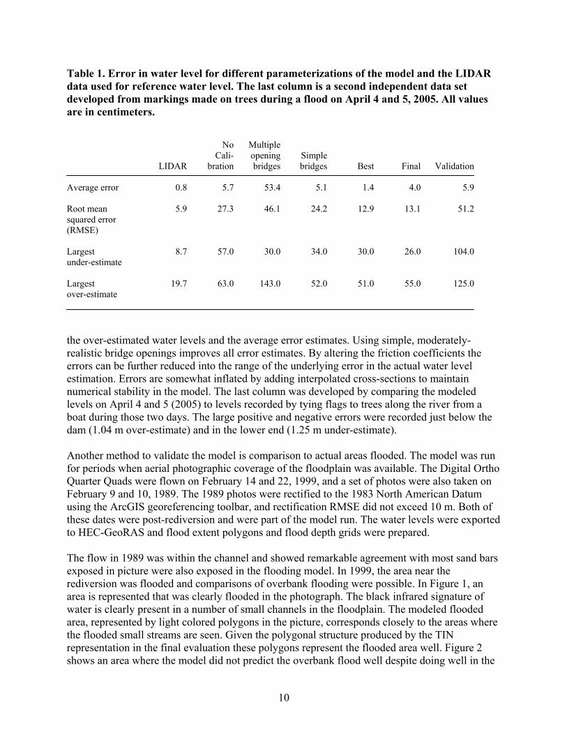
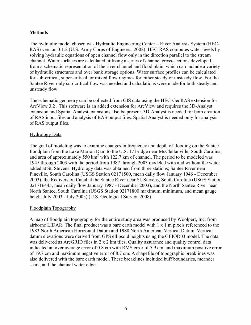
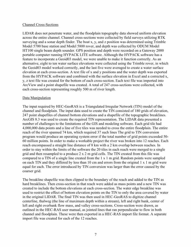
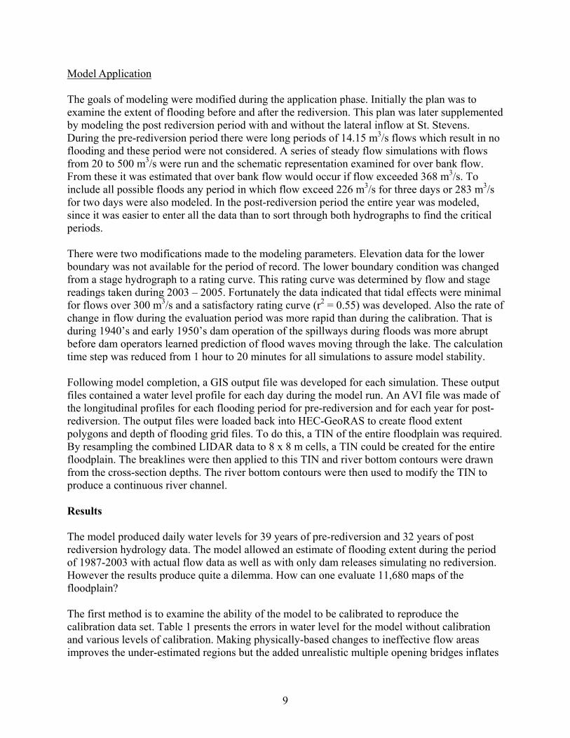
Table 1. Error in water level for different parameterizations of the model and the LIDAR data used for reference water level. The last column is a second independent data set developed from markings made on trees during a flood on April 4 and 5, 2005. All values are in centimeters. No Multiple Cali- opening Simple LIDAR bration bridges bridges Best Final Validation Average error 0.8 5.7 53.4 5.1 1.4 4.0 5.9 Root mean 5.9 27.3 46.1 24.2 12.9 13.1 51.2 squared error (RMSE) Largest 8.7 57.0 30.0 34.0 30.0 26.0 104.0 under-estimate Largest 19.7 63.0 143.0 52.0 51.0 55.0 125.0 over-estimate the over-estimated water levels and the average error estimates. Using simple, moderately-realistic bridge openings improves all error estimates. By altering the friction coefficients the errors can be further reduced into the range of the underlying error in the actual water level estimation. Errors are somewhat inflated by adding interpolated cross-sections to maintain numerical stability in the model. The last column was developed by comparing the modeled levels on April 4 and 5 (2005) to levels recorded by tying flags to trees along the river from a boat during those two days. The large positive and negative errors were recorded just below the dam (1.04 m over-estimate) and in the lower end (1.25 m under-estimate). Another method to validate the model is comparison to actual areas flooded. The model was run for periods when aerial photographic coverage of the floodplain was available. The Digital Ortho Quarter Quads were flown on February 14 and 22, 1999, and a set of photos were also taken on February 9 and 10, 1989. The 1989 photos were rectified to the 1983 North American Datum using the ArcGIS georeferencing toolbar, and rectification RMSE did not exceed 10 m. Both of these dates were post-rediversion and were part of the model run. The water levels were exported to HEC-GeoRAS and flood extent polygons and flood depth grids were prepared. The flow in 1989 was within the channel and showed remarkable agreement with most sand bars exposed in picture were also exposed in the flooding model. In 1999, the area near the rediversion was flooded and comparisons of overbank flooding were possible. In Figure 1, an area is represented that was clearly flooded in the photograph. The black infrared signature of water is clearly present in a number of small channels in the floodplain. The modeled flooded area, represented by light colored polygons in the picture, corresponds closely to the areas where the flooded small streams are seen. Given the polygonal structure produced by the TIN representation in the final evaluation these polygons represent the flooded area well. Figure 2 shows an area where the model did not predict the overbank flood well despite doing well in the

10

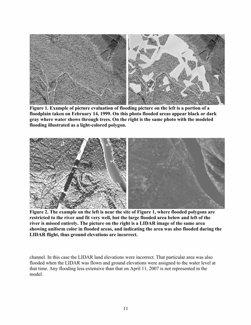
Figure 1. Example of picture evaluation of flooding picture on the left is a portion of a floodplain taken on February 14, 1999. On this photo flooded areas appear black or dark gray where water shows through trees. On the right is the same photo with the modeled flooding illustrated as a light-colored polygon.

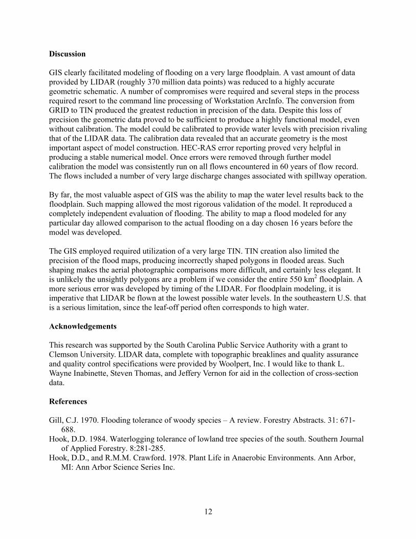
Figure 2. The example on the left is near the site of Figure 1, where flooded polygons are restricted to the river and fit very well, but the large flooded area below and left of the river is missed entirely. The picture on the right is a LIDAR image of the same area showing uniform color in flooded areas, and indicating the area was also flooded during the LIDAR flight, thus ground elevations are incorrect. channel. In this case the LIDAR land elevations were incorrect. That particular area was also flooded when the LIDAR was flown and ground elevations were assigned to the water level at that time. Any flooding less extensive than that on April 11, 2007 is not represented in the model.

11

Discussion GIS clearly facilitated modeling of flooding on a very large floodplain. A vast amount of data provided by LIDAR (roughly 370 million data points) was reduced to a highly accurate geometric schematic. A number of compromises were required and several steps in the process required resort to the command line processing of Workstation ArcInfo. The conversion from GRID to TIN produced the greatest reduction in precision of the data. Despite this loss of precision the geometric data proved to be sufficient to produce a highly functional model, even without calibration. The model could be calibrated to provide water levels with precision rivaling that of the LIDAR data. The calibration data revealed that an accurate geometry is the most important aspect of model construction. HEC-RAS error reporting proved very helpful in producing a stable numerical model. Once errors were removed through further model calibration the model was consistently run on all flows encountered in 60 years of flow record. The flows included a number of very large discharge changes associated with spillway operation. By far, the most valuable aspect of GIS was the ability to map the water level results back to the floodplain. Such mapping allowed the most rigorous validation of the model. It reproduced a completely independent evaluation of flooding. The ability to map a flood modeled for any particular day allowed comparison to the actual flooding on a day chosen 16 years before the model was developed. The GIS employed required utilization of a very large TIN. TIN creation also limited the precision of the flood maps, producing incorrectly shaped polygons in flooded areas. Such shaping makes the aerial photographic comparisons more difficult, and certainly less elegant. It is unlikely the unsightly polygons are a problem if we consider the entire 550 km2 floodplain. A more serious error was developed by timing of the LIDAR. For floodplain modeling, it is imperative that LIDAR be flown at the lowest possible water levels. In the southeastern U.S. that is a serious limitation, since the leaf-off period often corresponds to high water. Acknowledgements This research was supported by the South Carolina Public Service Authority with a grant to Clemson University. LIDAR data, complete with topographic breaklines and quality assurance and quality control specifications were provided by Woolpert, Inc. I would like to thank L. Wayne Inabinette, Steven Thomas, and Jeffery Vernon for aid in the collection of cross-section data. References Gill, C.J. 1970. Flooding tolerance of woody species – A review. Forestry Abstracts. 31: 671-

688. Hook, D.D. 1984. Waterlogging tolerance of lowland tree species of the south. Southern Journal

of Applied Forestry. 8:281-285. Hook, D.D., and R.M.M. Crawford. 1978. Plant Life in Anaerobic Environments. Ann Arbor,

MI: Ann Arbor Science Series Inc.

12

Hosner, J.F. 1960. Relative tolerance to complete inundation of fourteen bottomland tree species. Forest Science. 6: 67-77.

Patterson, G.G., G.K. Speiran, and B.H. Whetstone. 1985. Hydrology and its effects on distribution of vegetation in Congaree Swamp National Monument, South Carolina. Water-Resources Investigations Report 85-4256. Columbia, SC: U.S. Geological Survey.

Rikard, M. 1988. Hydrologic and vegetative relationships of Congaree Swamp National Monument. PhD dissertation. Clemson SC: Clemson University.

Seaber, P.R., F.P. Kapinos, and G.L. Knapp. 1987. Hydrologic unit maps. U.S. Geological Survey Water-Supply Paper 2294. Denver, CO: U.S. Geological Survey. Available at: http://pubs.usgs.gov/wsp/wsp2294/. Accessed 20 April 2008.

U.S. Army Corps of Engineers. 2002. HEC-RAS River Analysis System. Available at: http://www.hec.usace.army.mil/software/hec-ras/hecras-hecras.html. Accessed 20 April 2008.

U.S. Geological Survey. 2008. Daily Data for South Carolina: Stage and Streamflow. Available at: http://waterdata.usgs.gov/sc/nwis/current/?type=dailysd. Accessed 20 April 2008.

13