N.E. Leonard – MBARI – August 1, 2006Slide 1/46

Cooperative Control and Mobile Sensor Networks in the Ocean

Naomi Ehrich LeonardMechanical & Aerospace Engineering

Princeton Universitynaomi@princeton.edu, www.princeton.edu/~naomi

Derek Paley (grad student), Francois Lekien, Fumin Zhang (post-docs)Dave Fratantoni and John Lund (Woods Hole Oceanographic Inst.)Russ Davis (Scripps Inst. Oceanography) Rodolphe Sepulchre (University of Liege, Belgium)

Collaborators:

N.E. Leonard – MBARI – August 1, 2006Slide 2/46

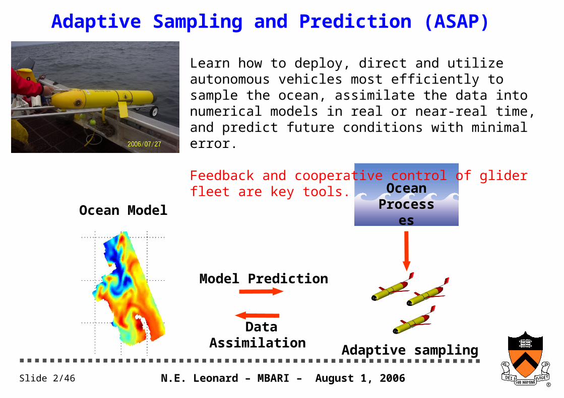
Adaptive Sampling and Prediction (ASAP)

Ocean ProcessesOcean Model

Model Prediction

Data Assimilation

Adaptive sampling

Learn how to deploy, direct and utilize autonomous vehicles most efficiently to sample the ocean, assimilate the data into numerical models in real or near-real time, and predict future conditions with minimal error.

Feedback and cooperative control of glider fleet are key tools.

N.E. Leonard – MBARI – August 1, 2006Slide 3/46

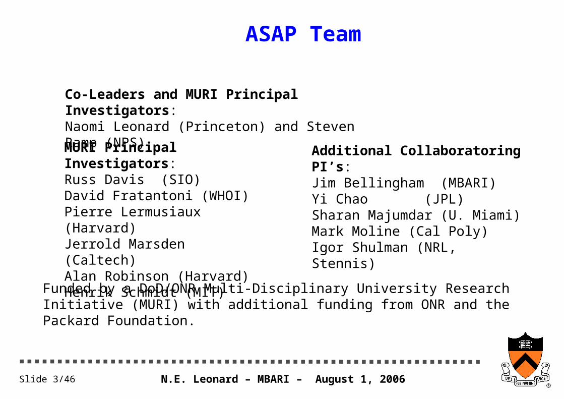
ASAP Team

Additional Collaboratoring PI’s:Jim Bellingham (MBARI)Yi Chao (JPL)Sharan Majumdar (U. Miami)Mark Moline (Cal Poly)Igor Shulman (NRL, Stennis)

MURI Principal Investigators:Russ Davis (SIO)David Fratantoni (WHOI)Pierre Lermusiaux (Harvard)Jerrold Marsden (Caltech)Alan Robinson (Harvard)Henrik Schmidt (MIT)

Co-Leaders and MURI Principal Investigators:Naomi Leonard (Princeton) and Steven Ramp (NPS)

Funded by a DoD/ONR Multi-Disciplinary University Research Initiative (MURI) with additional funding from ONR and the Packard Foundation.

N.E. Leonard – MBARI – August 1, 2006Slide 4/46

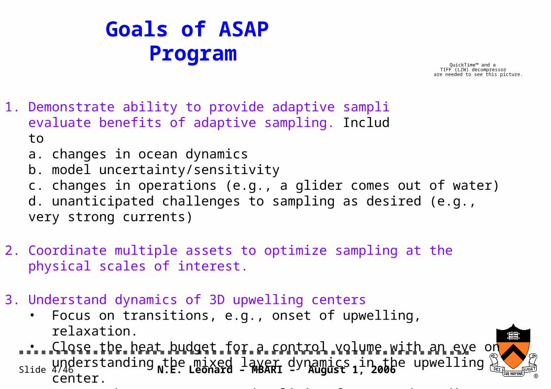
Goals of ASAP Program

1. Demonstrate ability to provide adaptive sampling and evaluate benefits of adaptive sampling. Includes responding to a. changes in ocean dynamics b. model uncertainty/sensitivityc. changes in operations (e.g., a glider comes out of water)d. unanticipated challenges to sampling as desired (e.g., very strong currents)

2. Coordinate multiple assets to optimize sampling at the physical scales of interest.

3. Understand dynamics of 3D upwelling centers• Focus on transitions, e.g., onset of upwelling, relaxation.• Close the heat budget for a control volume with an eye on understanding the

mixed layer dynamics in the upwelling center.• Locate the temperature and salinity fronts and predict acoustic propagation.

QuickTime™ and aTIFF (LZW) decompressor

are needed to see this picture.

N.E. Leonard – MBARI – August 1, 2006Slide 5/46

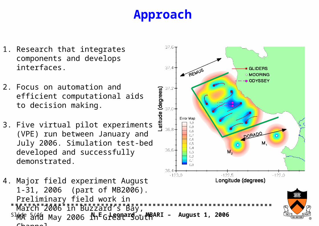
Approach

1. Research that integrates components and develops interfaces.

2. Focus on automation and efficient computational aids to decision making.

3. Five virtual pilot experiments (VPE) run between January and July 2006. Simulation test-bed developed and successfully demonstrated.

4. Major field experiment August 1-31, 2006 (part of MB2006). Preliminary field work in March 2006 in Buzzard’s Bay, MA and May 2006 in Great South Channel.

N.E. Leonard – MBARI – August 1, 2006Slide 6/46

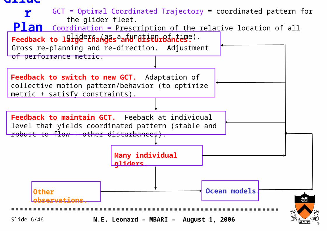
Glider Plan

Feedback to large changes and disturbances. Gross re-planning and re-direction. Adjustment of performance metric.

Feedback to switch to new GCT. Adaptation of collective motion pattern/behavior (to optimize metric + satisfy constraints).

Feedback to maintain GCT. Feeback at individual level that yields coordinated pattern (stable and robust to flow + other disturbances).

Many individual gliders.

Other observations. Ocean models.

GCT = Optimal Coordinated Trajectory = coordinated pattern for the glider fleet.Coordination = Prescription of the relative location of all gliders (as a function of time).

N.E. Leonard – MBARI – August 1, 2006Slide 7/46

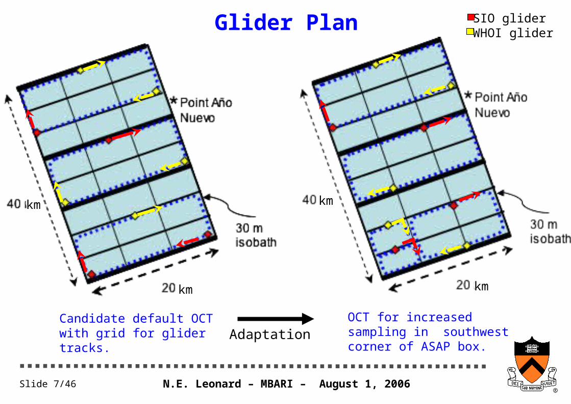
Glider Plan

OCT for increased sampling in southwest corner of ASAP box.

Candidate default OCT with grid for glider tracks. Adaptation

SIO gliderWHOI glider

km km

kmkm

N.E. Leonard – MBARI – August 1, 2006Slide 8/46

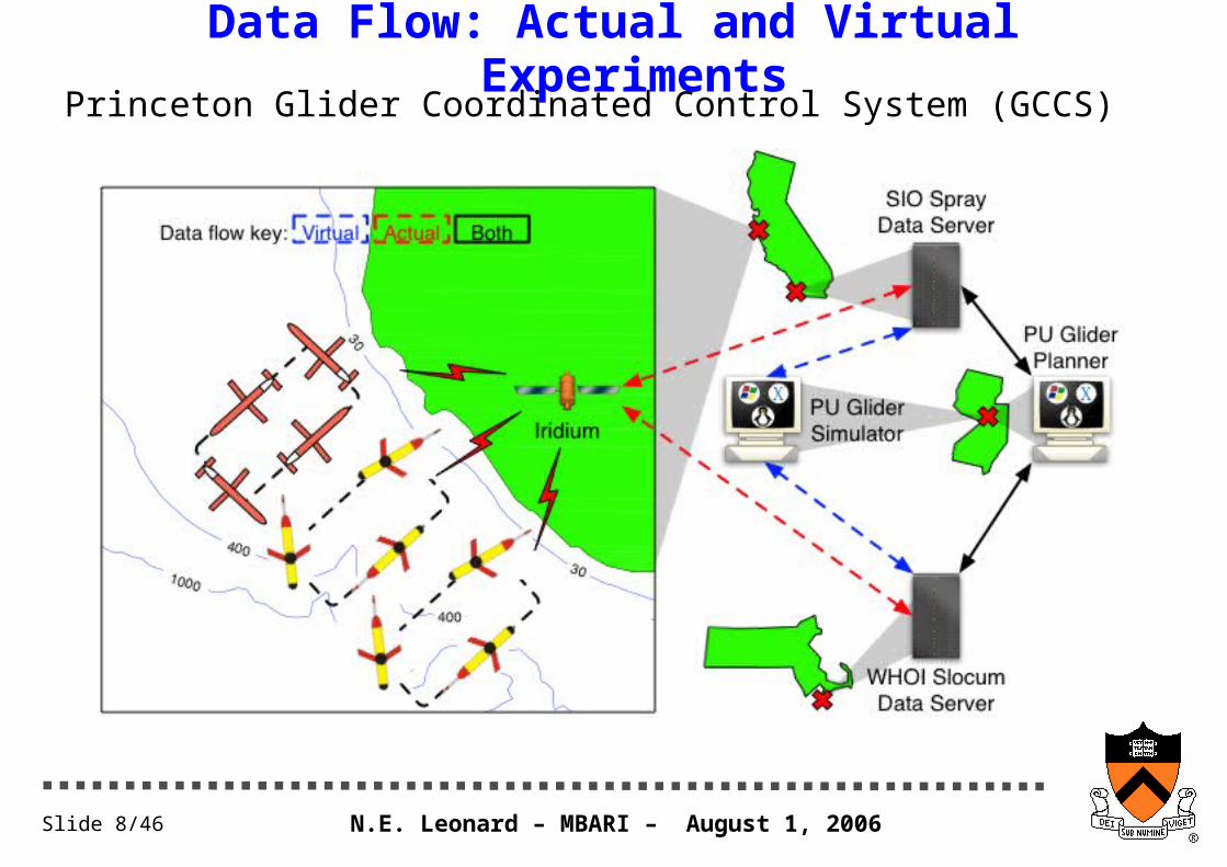
Data Flow: Actual and Virtual ExperimentsPrinceton Glider Coordinated Control System (GCCS)

N.E. Leonard – MBARI – August 1, 2006Slide 9/46

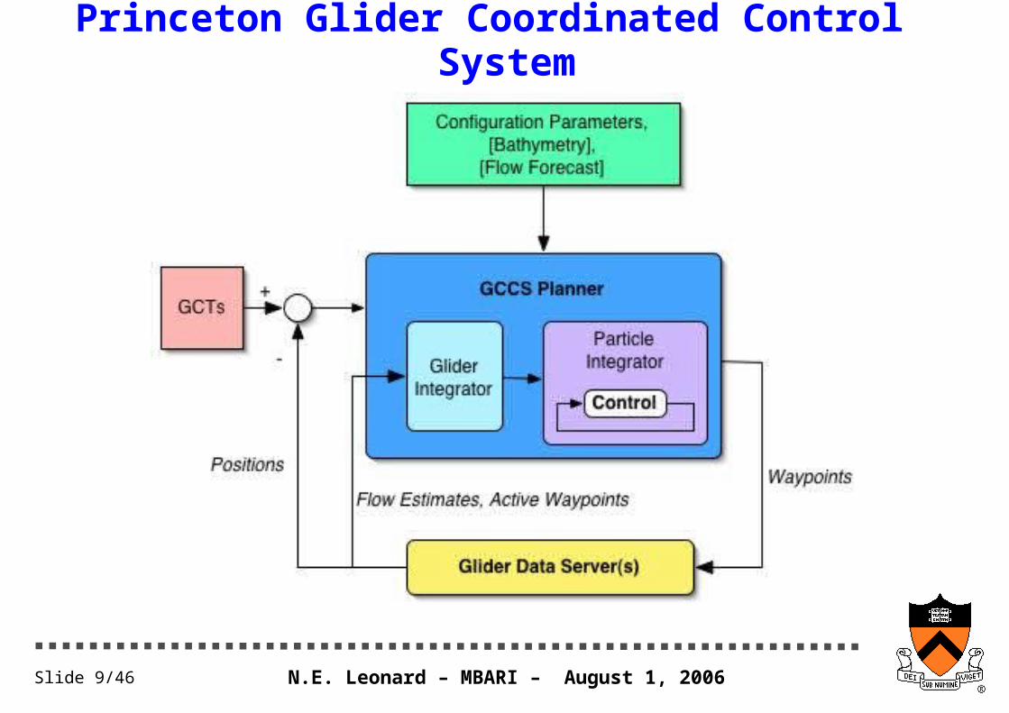
Princeton Glider Coordinated Control System

N.E. Leonard – MBARI – August 1, 2006Slide 10/46

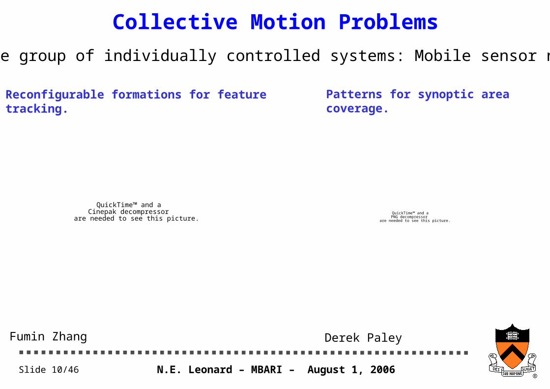
Collective Motion Problems

Coordinate group of individually controlled systems: Mobile sensor networks

QuickTime™ and aCinepak decompressor

are needed to see this picture.

Fumin Zhang Derek Paley

QuickTime™ and aPNG decompressor

are needed to see this picture.

Reconfigurable formations for feature tracking. Patterns for synoptic area coverage.

N.E. Leonard – MBARI – August 1, 2006Slide 11/46

Patterns for Synoptic Area Coverage

Sampling metric

Optimization of coordinated tracks

Coordinated control of mobile sensors onto tracks

Cooperative estimate of flow field which influences motion of mobile sensors.

Adaptation of coordinated tracks

N.E. Leonard – MBARI – August 1, 2006Slide 12/46

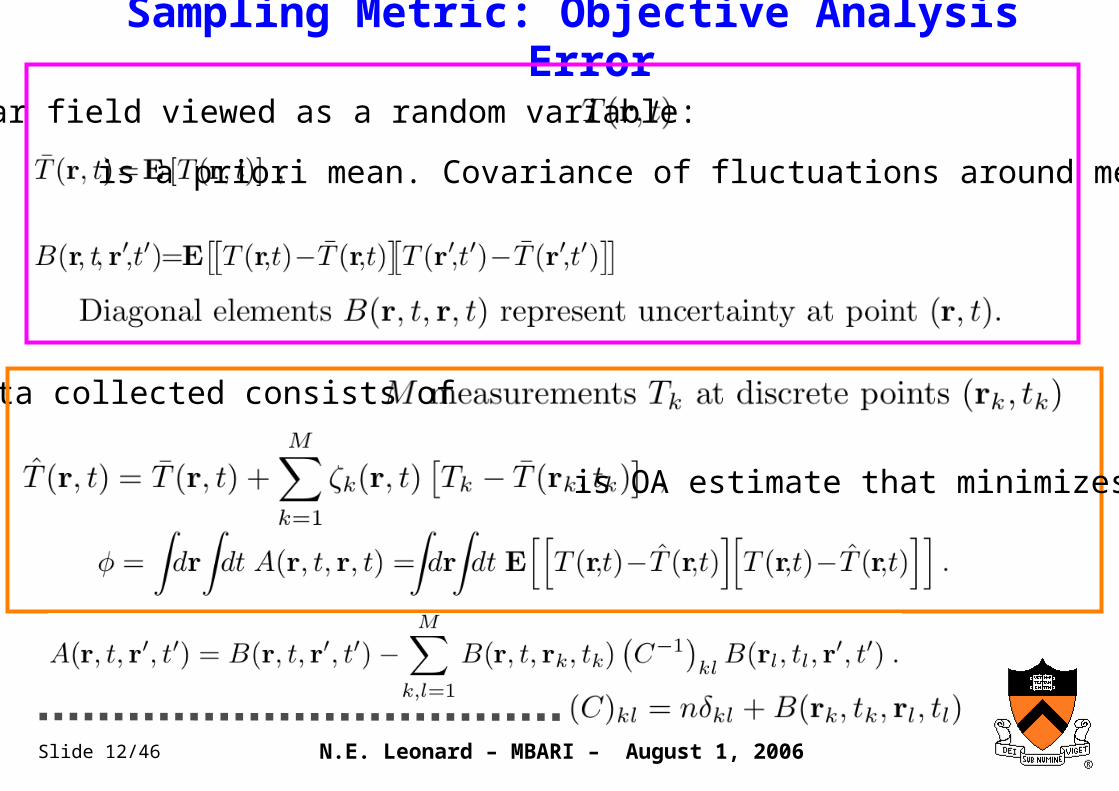
Sampling Metric: Objective Analysis Error

Scalar field viewed as a random variable:

Data collected consists of

is OA estimate that minimizes

is a priori mean. Covariance of fluctuations around mean is

N.E. Leonard – MBARI – August 1, 2006Slide 13/46

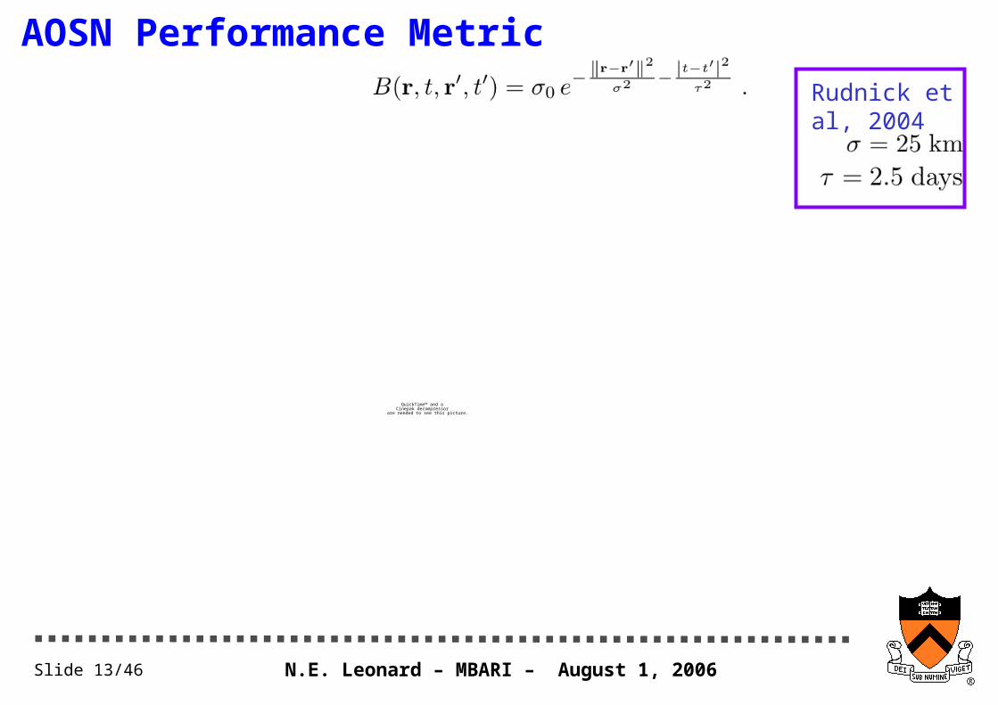
AOSN Performance Metric

QuickTime™ and aCinepak decompressor

are needed to see this picture.

Rudnick et al, 2004

N.E. Leonard – MBARI – August 1, 2006Slide 14/46

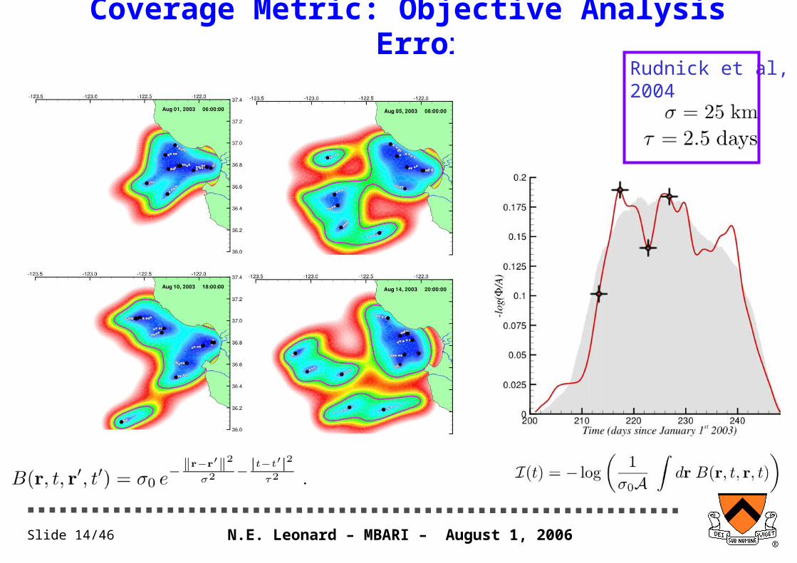
Coverage Metric: Objective Analysis ErrorRudnick et al, 2004

N.E. Leonard – MBARI – August 1, 2006Slide 15/46

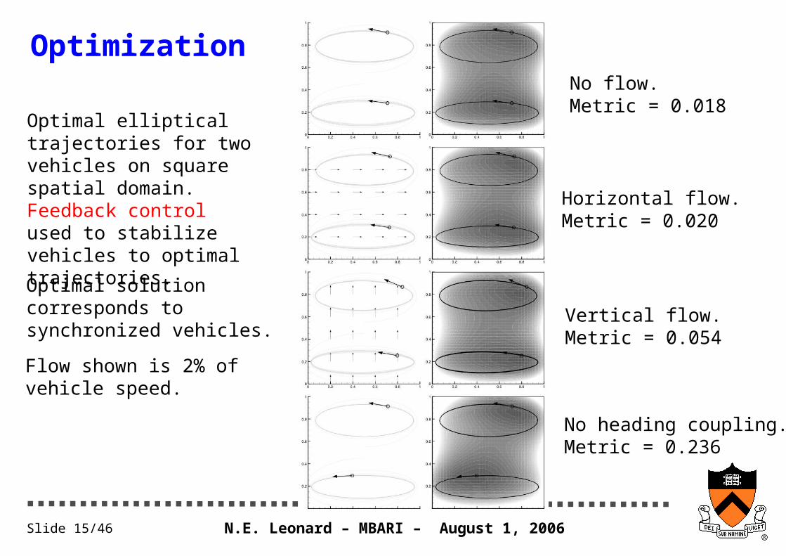
Optimization

Optimal elliptical trajectories for two vehicles on square spatial domain. Feedback control used to stabilize vehicles to optimal trajectories.

Optimal solution corresponds to synchronized vehicles.

Flow shown is 2% of vehicle speed.

No flow. Metric = 0.018

Horizontal flow. Metric = 0.020

Vertical flow. Metric = 0.054

No heading coupling. Metric = 0.236

N.E. Leonard – MBARI – August 1, 2006Slide 16/46

Collective Motion for Mobile Sensor Networks

Sensor platforms coordinate motion on patterns so data collected minimizes uncertainty in sampled field.

QuickTime™ and aMS-MPEG4v2 Codec decompressor

are needed to see this picture.

N.E. Leonard – MBARI – August 1, 2006Slide 17/46

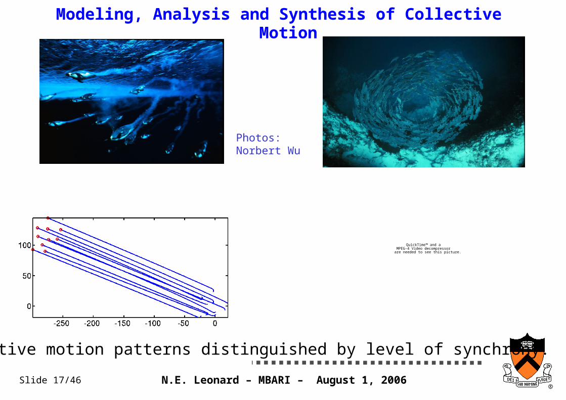
Modeling, Analysis and Synthesis of Collective Motion

QuickTime™ and aMPEG-4 Video decompressor

are needed to see this picture.

Collective motion patterns distinguished by level of synchrony.

Photos:Norbert Wu

N.E. Leonard – MBARI – August 1, 2006Slide 18/46

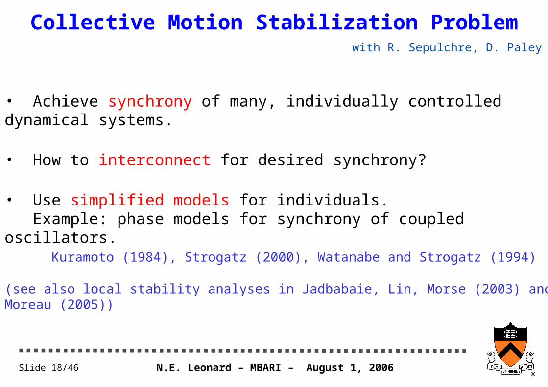
Collective Motion Stabilization Problem

• Achieve synchrony of many, individually controlled dynamical systems.

• How to interconnect for desired synchrony?

• Use simplified models for individuals. Example: phase models for synchrony of coupled oscillators.

Kuramoto (1984), Strogatz (2000), Watanabe and Strogatz (1994) (see also local stability analyses in Jadbabaie, Lin, Morse (2003) and Moreau (2005))

with R. Sepulchre, D. Paley

N.E. Leonard – MBARI – August 1, 2006Slide 19/46

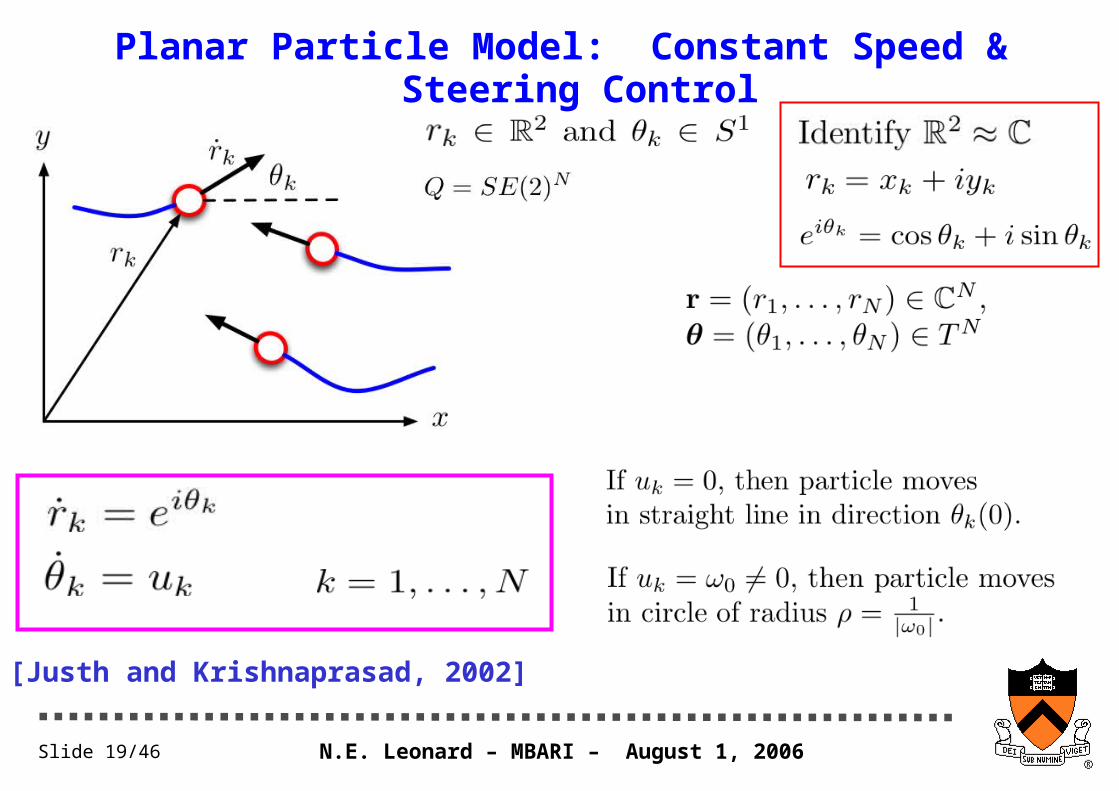
Planar Particle Model: Constant Speed & Steering Control

[Justh and Krishnaprasad, 2002]

N.E. Leonard – MBARI – August 1, 2006Slide 20/46

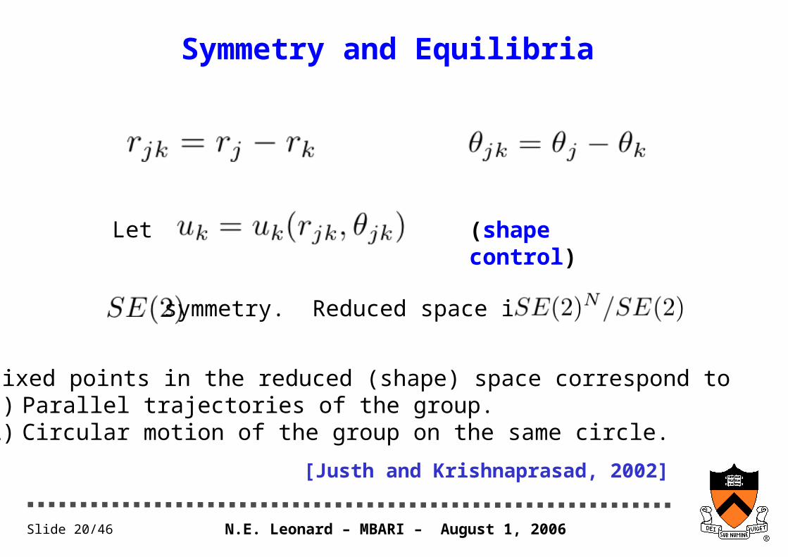
Symmetry and Equilibria

symmetry. Reduced space is

Fixed points in the reduced (shape) space correspond to 1) Parallel trajectories of the group.2) Circular motion of the group on the same circle.

[Justh and Krishnaprasad, 2002]

Let (shape control)

N.E. Leonard – MBARI – August 1, 2006Slide 21/46

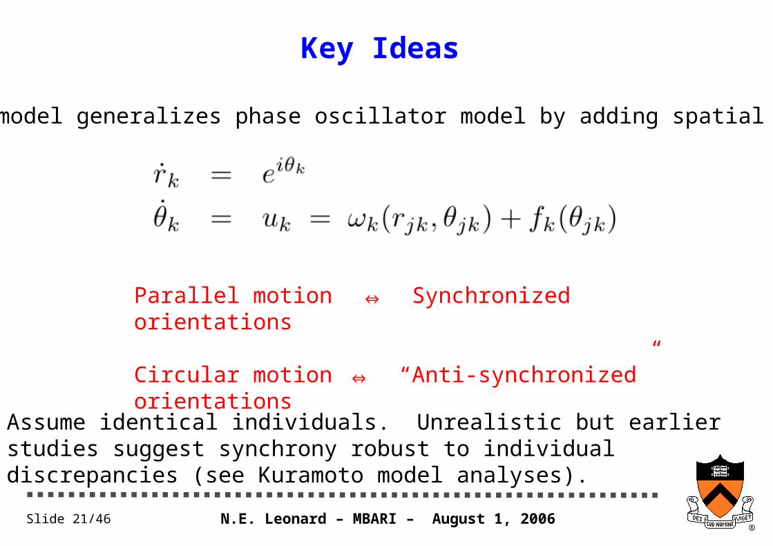
Key Ideas

Particle model generalizes phase oscillator model by adding spatial dynamics:

Parallel motion ⇔ Synchronized orientations

Circular motion ⇔ “Anti-synchronized” orientations

Assume identical individuals. Unrealistic but earlier studies suggest synchrony robust to individual discrepancies (see Kuramoto model analyses).

N.E. Leonard – MBARI – August 1, 2006Slide 22/46

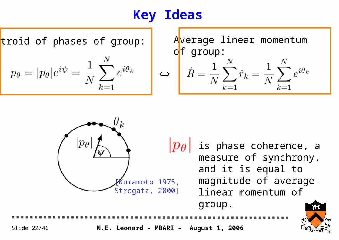
Key Ideas

is phase coherence, a measure of synchrony, and it is equal to magnitude of average linear momentum of group.[Kuramoto 1975,

Strogatz, 2000]

Average linear momentumof group:

Centroid of phases of group:

N.E. Leonard – MBARI – August 1, 2006Slide 23/46

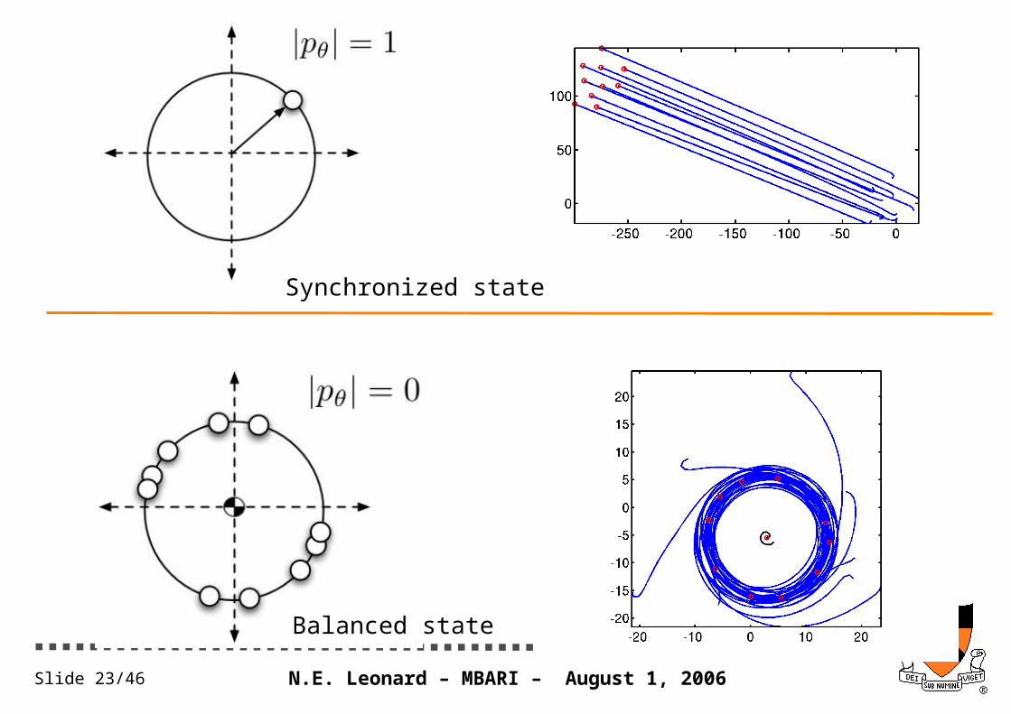
Synchronized state

Balanced state

N.E. Leonard – MBARI – August 1, 2006Slide 24/46

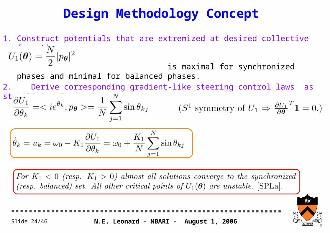
Design Methodology Concept

1. Construct potentials that are extremized at desired collective formations.

is maximal for synchronized phases and minimal for balanced phases.

2. Derive corresponding gradient-like steering control laws as stabilizing feedback:

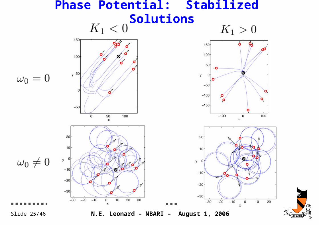
N.E. Leonard – MBARI – August 1, 2006Slide 25/46

Phase Potential: Stabilized Solutions

N.E. Leonard – MBARI – August 1, 2006Slide 26/46

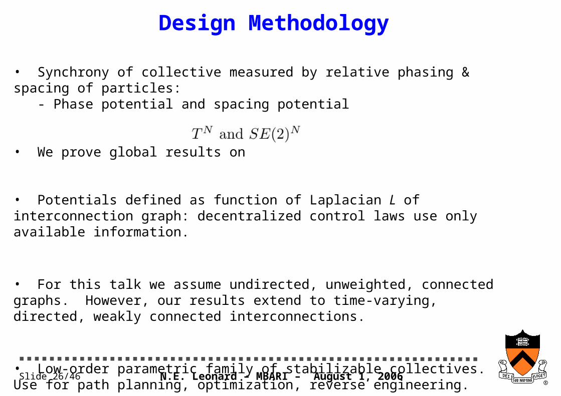
• Synchrony of collective measured by relative phasing & spacing of particles: - Phase potential and spacing potential

• We prove global results on

• Potentials defined as function of Laplacian L of interconnection graph: decentralized control laws use only available information.

• For this talk we assume undirected, unweighted, connected graphs. However, our results extend to time-varying, directed, weakly connected interconnections.

• Low-order parametric family of stabilizable collectives. Use for path planning, optimization, reverse engineering.

Design Methodology

N.E. Leonard – MBARI – August 1, 2006Slide 27/46

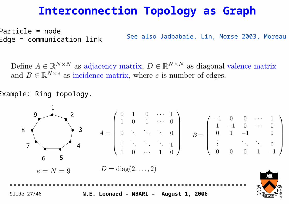
Interconnection Topology as Graph

Example: Ring topology.

1

7

8

6 5

2

4

9

3

Particle = node Edge = communication link See also Jadbabaie, Lin, Morse 2003, Moreau 2005

N.E. Leonard – MBARI – August 1, 2006Slide 28/46

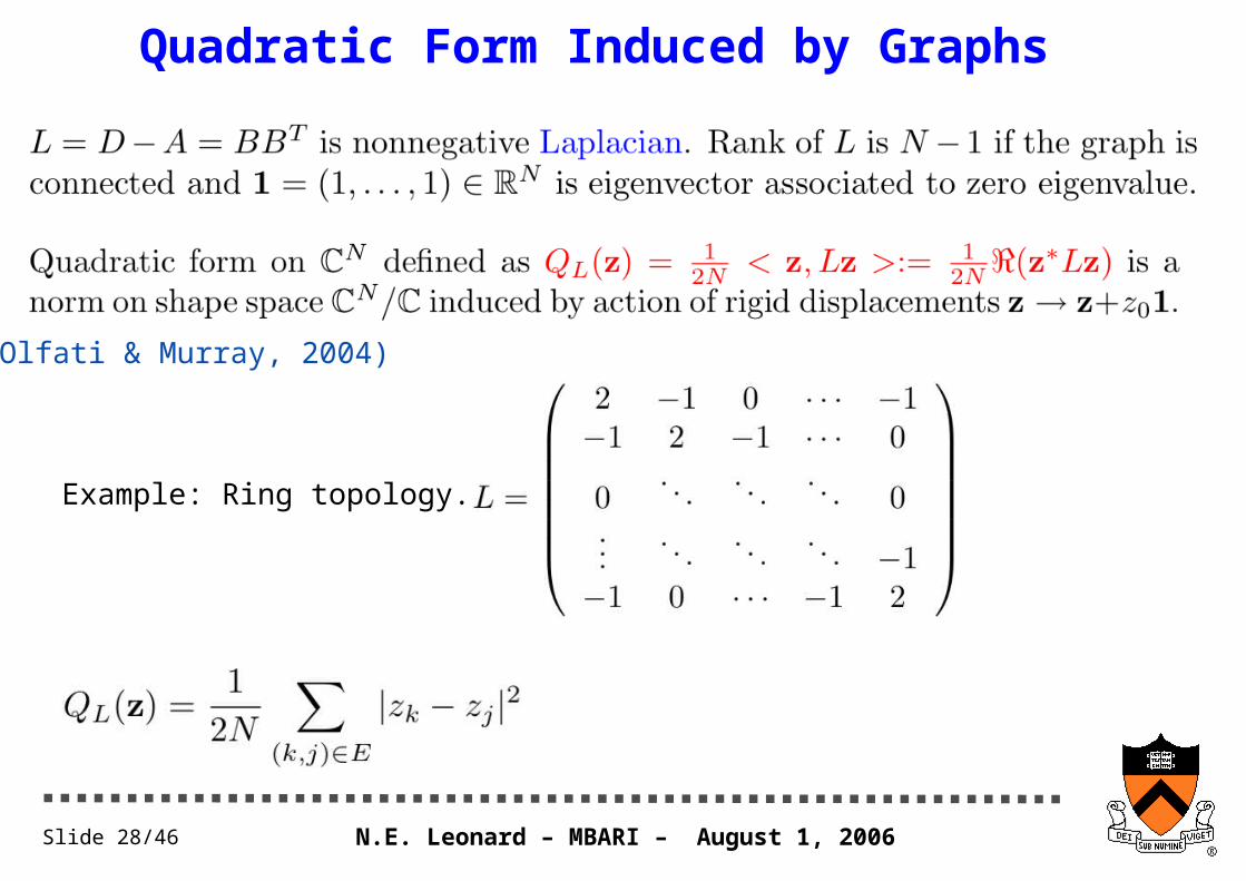
Quadratic Form Induced by Graphs

Example: Ring topology.

(Olfati & Murray, 2004)

N.E. Leonard – MBARI – August 1, 2006Slide 29/46

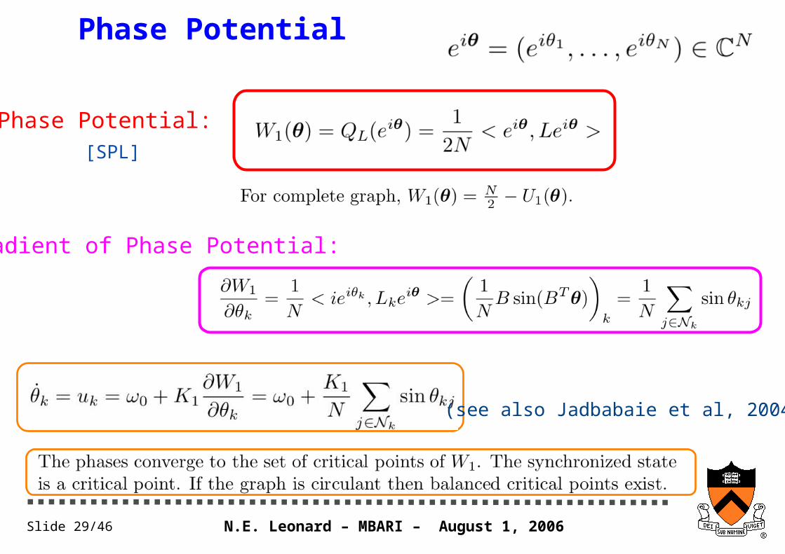
Phase Potential

Phase Potential:

Gradient of Phase Potential:

[SPL]

(see also Jadbabaie et al, 2004)

N.E. Leonard – MBARI – August 1, 2006Slide 30/46

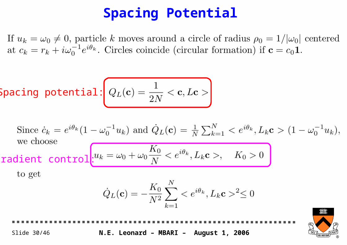
Spacing Potential

Spacing potential:

Gradient control:

N.E. Leonard – MBARI – August 1, 2006Slide 31/46

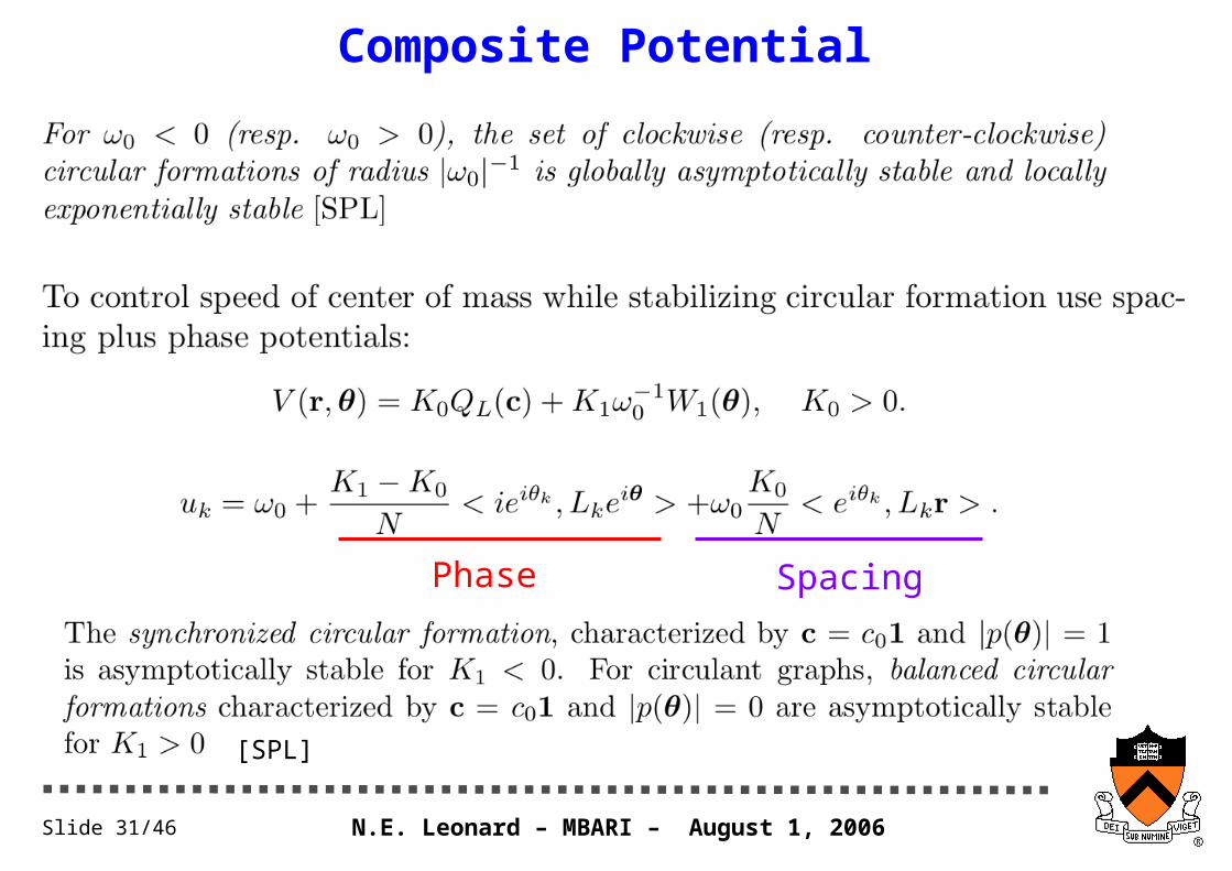
Composite Potential

SpacingPhase

[SPL]

N.E. Leonard – MBARI – August 1, 2006Slide 32/46

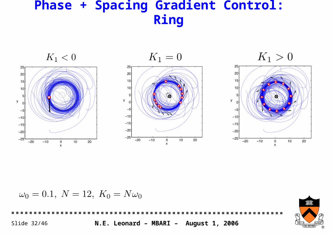
Phase + Spacing Gradient Control: Ring

N.E. Leonard – MBARI – August 1, 2006Slide 33/46

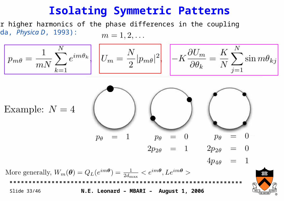
Isolating Symmetric PatternsConsider higher harmonics of the phase differences in the coupling (K. Okuda, Physica D, 1993):

2

N.E. Leonard – MBARI – August 1, 2006Slide 34/46

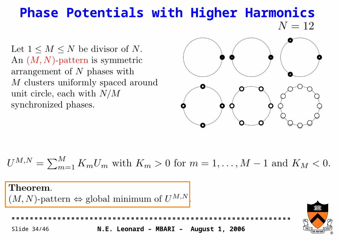
Phase Potentials with Higher Harmonics

N.E. Leonard – MBARI – August 1, 2006Slide 35/46

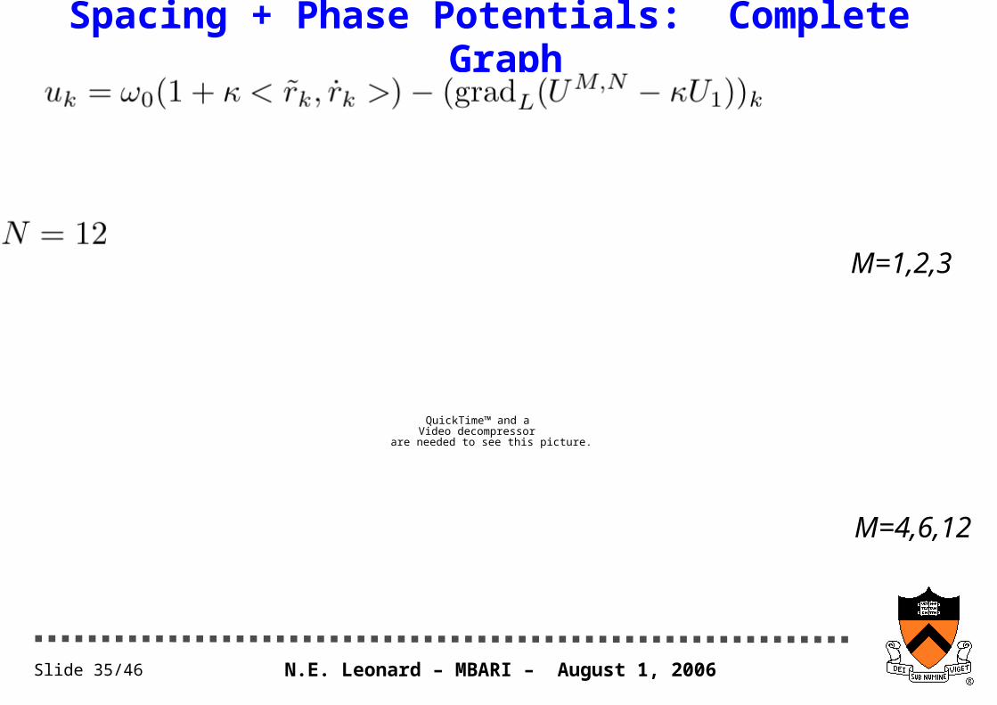
Spacing + Phase Potentials: Complete Graph

QuickTime™ and aVideo decompressor

are needed to see this picture.

M=1,2,3

M=4,6,12

N.E. Leonard – MBARI – August 1, 2006Slide 36/46

Multi-Scale and Multi-Graph

QuickTime™ and aMS-MPEG4v2 Codec decompressor

are needed to see this picture.

N.E. Leonard – MBARI – August 1, 2006Slide 37/46

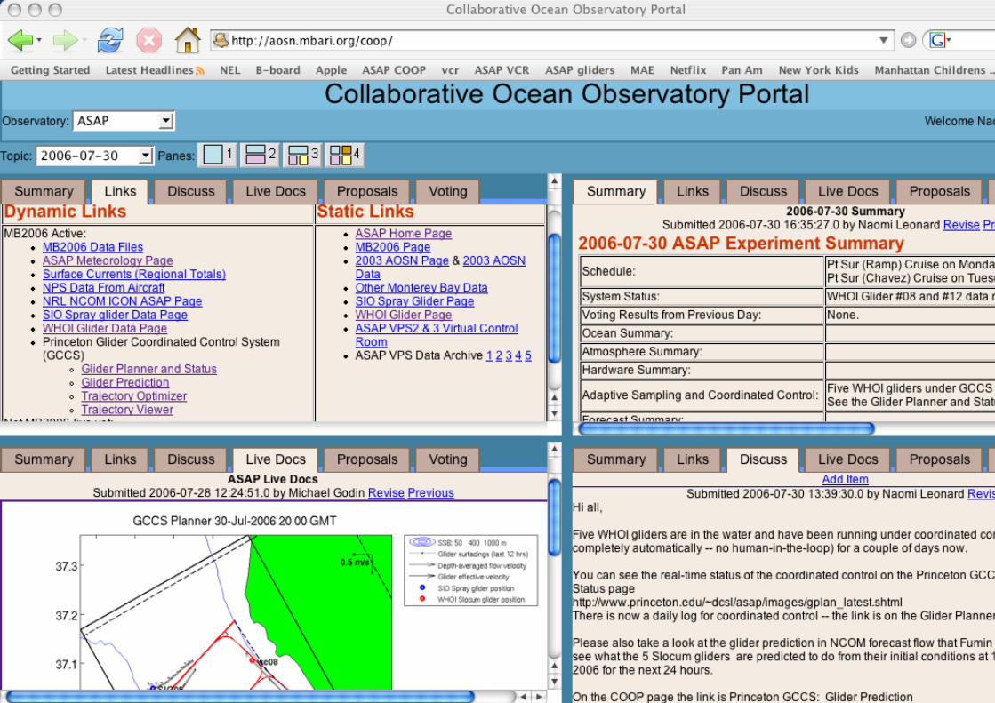
ASAP Virtual Control Room

N.E. Leonard – MBARI – August 1, 2006Slide 38/46

N.E. Leonard – MBARI – August 1, 2006Slide 39/46

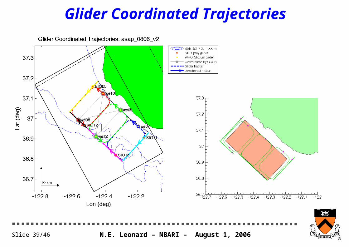
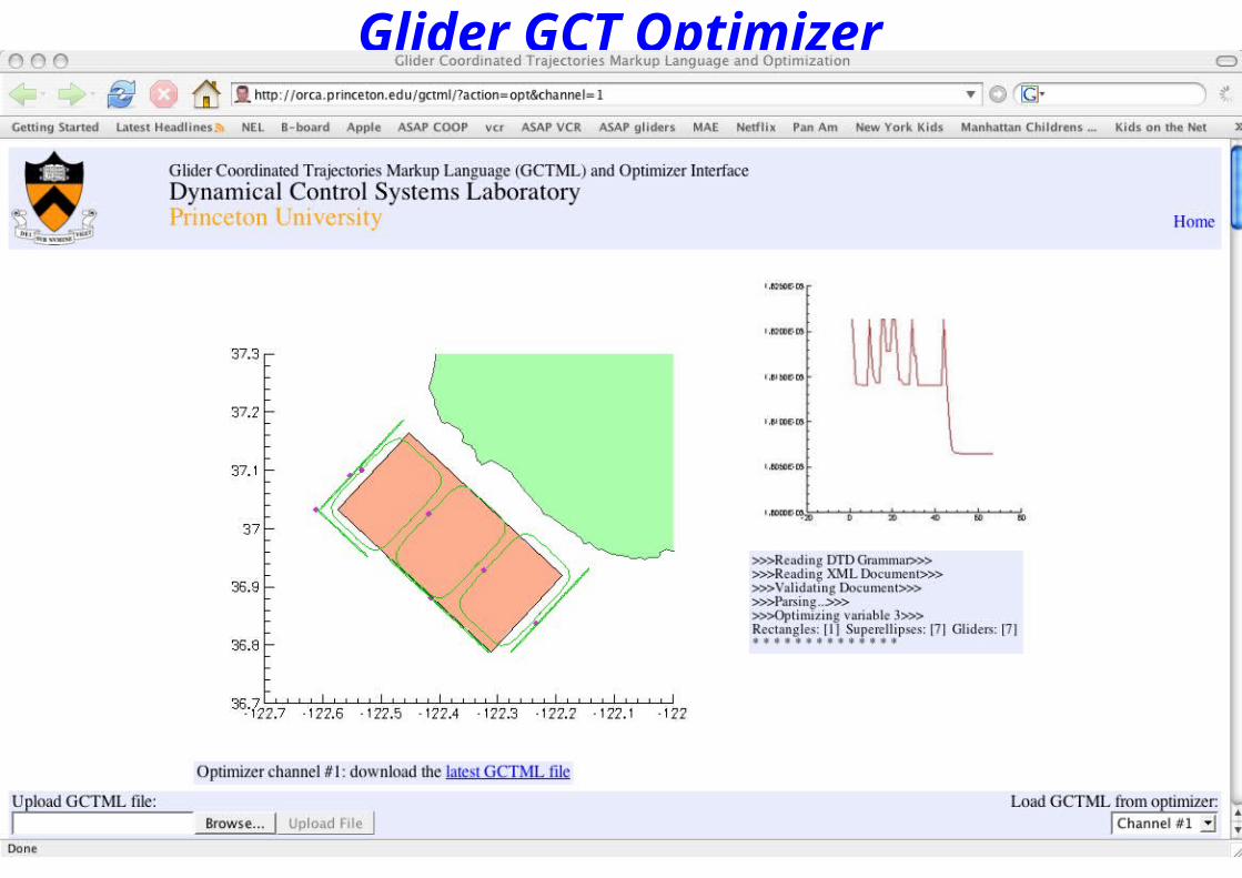
Glider Coordinated Trajectories

N.E. Leonard – MBARI – August 1, 2006Slide 40/46

Glider GCT Optimizer

N.E. Leonard – MBARI – August 1, 2006Slide 41/46

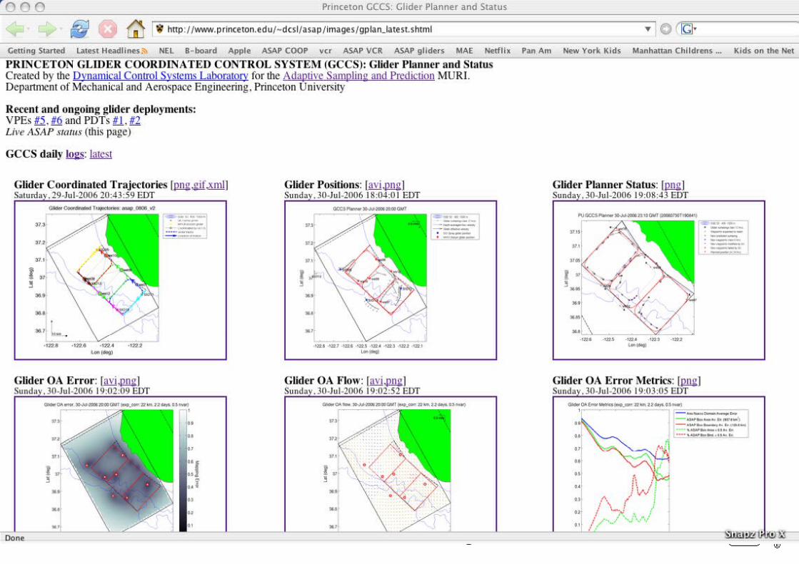
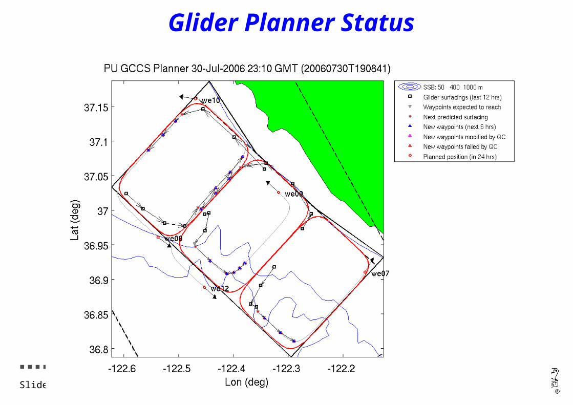
Glider Planner Status

N.E. Leonard – MBARI – August 1, 2006Slide 42/46

Glider Positions

QuickTime™ and aMS-MPEG4v2 Codec decompressor

are needed to see this picture.

N.E. Leonard – MBARI – August 1, 2006Slide 43/46

Glider Prediction

QuickTime™ and aMS-MPEG4v2 Codec decompressor

are needed to see this picture.

N.E. Leonard – MBARI – August 1, 2006Slide 44/46

Glider OA Error Map

QuickTime™ and aMS-MPEG4v2 Codec decompressor

are needed to see this picture.

N.E. Leonard – MBARI – August 1, 2006Slide 45/46

Glider OA Flow

QuickTime™ and aMS-MPEG4v2 Codec decompressor

are needed to see this picture.

N.E. Leonard – MBARI – August 1, 2006Slide 46/46

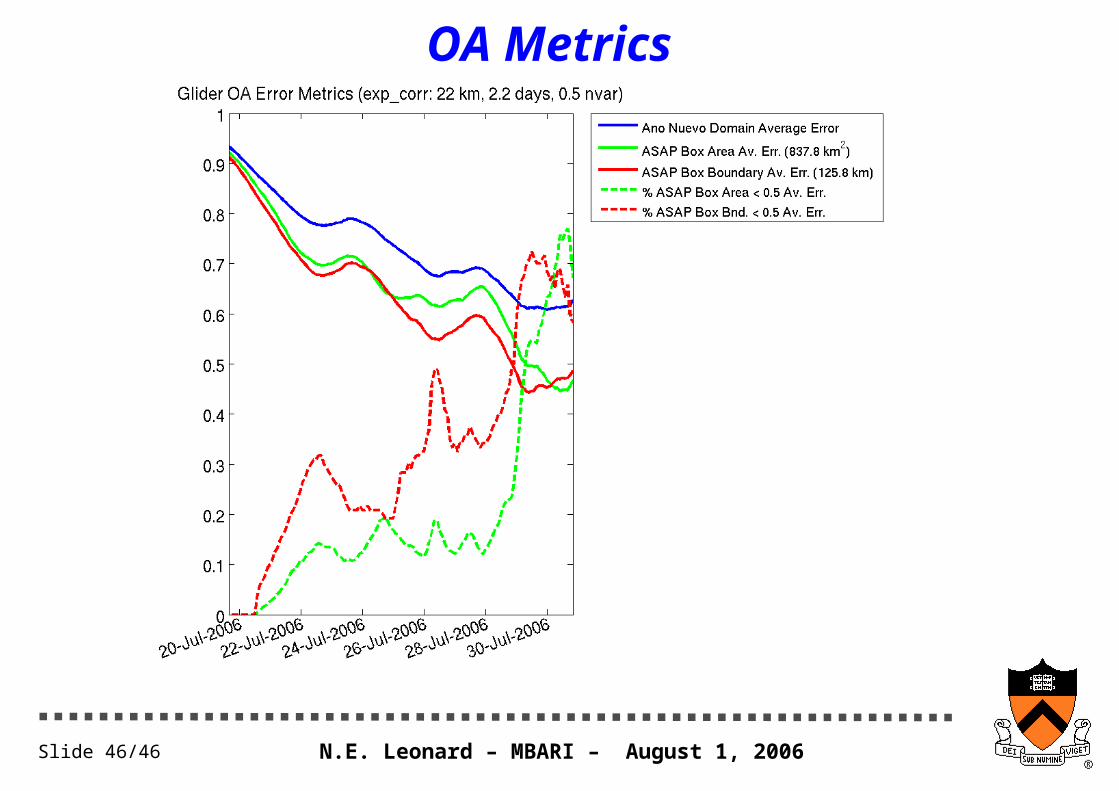
OA Metrics

N.E. Leonard – MBARI – August 1, 2006Slide 47/46

Final Remarks

Derived simply parameterized family of stabilizable collective motions.

Optimization of collective behavior (motion, sampling) given constraints of system (energy, communication) and challenges of environment (obstacles, flow field).

Glider Coordinated Control System (GCCS) -- software suite for real and virtual experiments.

ASAP 2006 field experiment has begun. Five gliders under coordinated control that is fully automated (control running on computer at Princeton).