Near-Ground Rotation in Simulated Supercells: On the

Near-Ground Rotation in Simulated Supercells: On the Robustnessof the Baroclinic Mechanism*

JOHANNES M. L. DAHL

Atmospheric Science Group, Department of Geosciences, Texas Tech University, Lubbock, Texas

(Manuscript received 25 March 2015, in final form 26 August 2015)

ABSTRACT

This study addresses the robustness of the baroclinicmechanism that facilitates the onset of surface rotation

in supercells by using two idealized simulations with different microphysics parameterizations and by con-

sidering previous results. In particular, the importance of ambient crosswise vorticity relative to baroclinically

generated vorticity in the development of near-ground cyclonic vorticity is analyzed. The storms were sim-

ulated using the CM1model in a kinematic base state characterized by a straight-line hodograph. A trajectory

analysis spanning about 30min was performed for a large number of parcels that contribute to near-surface

vertical-vorticity maxima. The vorticity along these trajectories was decomposed into barotropic and non-

barotropic parts, where the barotropic vorticity represents the effects of the preexisting, substantially

crosswise horizontal storm-relative vorticity. The nonbarotropic part represents the vorticity produced baro-

clinically within the storm. It was found that the imported barotropic vorticity attains a downward com-

ponent near the surface, while the baroclinic vorticity points upward and dominates. This dominance of the

baroclinic vorticity is independent of whether a single-moment or double-moment microphysics parame-

terization is used. A scaling argument is offered as explanation, predicting that the baroclinic vertical

vorticity becomes increasingly dominant as downdraft strength increases.

1. Introduction

One of the outstanding questions in tornado research

remains the origin of ‘‘seed’’ ground-level rotation1 that

horizontal convergence can act upon to realize a com-

pact vortex (e.g., Davies-Jones et al. 2001). It has been

established that the onset of this initial rotation is due to

the rearrangement of initially horizontal vortex lines

within downdrafts (Davies-Jones and Brooks 1993;

Walko 1993; Wicker and Wilhelmson 1995; Adlerman

et al. 1999; Davies-Jones et al. 2001; Davies-Jones and

Markowski 2013; Dahl et al. 2014; Markowski et al.

2014; Schenkman et al. 2014; Parker and Dahl 2015),

assuming negligible preexisting vertical vorticity in the

storm’s environment. In general terms, these horizontal

vortex lines may either be generated within the storm by

buoyant or frictional torques, or the horizontal vorticity

may be imported into the downdraft from the environ-

ment. This study is part of an ongoing effort to explore

which of these contributions dominate in what situation,

which is crucial for a complete understanding of tornado

dynamics. In an attempt to tackle this problem, Dahl

et al. (2014) applied a vorticity decomposition technique

to quantify the roles of storm-generated and imported

vorticity in an idealized free-slip simulation of the Del

City, Oklahoma, supercell. They found that the imported

ambient vorticity (treated as ‘‘barotropic vorticity’’)

did not contribute much to the development of vertical-

vorticity maxima at the lowest model level. Rather, the

near-surface vertical vorticity originated primarily

from horizontal buoyancy torques within the storm.

This behavior is due to the orientation of the ambient

vorticity vector relative to the storm-relative flow:

if this barotropic vorticity is mostly streamwise it

* Supplemental information related to this paper is available at

the Journals Online website: http://dx.doi.org/10.1175/MWR-D-

15-0115.s1.

Corresponding author address: Johannes Dahl, Atmospheric

Science Group, Department of Geosciences, Texas Tech Univer-

sity, Box 41053, Lubbock, TX 79409.

E-mail: [email protected]

1 In this study, ‘‘ground level’’ rotation or ‘‘near ground’’ rota-

tion refer to rotation of air about a vertical axis an arbitrarily small

distance above the lower boundary.

DECEMBER 2015 DAHL 4929

DOI: 10.1175/MWR-D-15-0115.1

� 2015 American Meteorological SocietyUnauthenticated | Downloaded 04/08/22 06:27 PM UTC

http://dx.doi.org/10.1175/MWR-D-15-0115.s1

http://dx.doi.org/10.1175/MWR-D-15-0115.s1

mailto:[email protected]

will tend to remain aligned with the velocity vectors.

Hence, as the trajectories turn on the horizontal plane

near the ground, the barotropic vorticity likewise turns

horizontally and thus cannot contribute to vertical near-

ground vorticity, as already anticipated by Davies-Jones

and Brooks (1993) and Davies-Jones et al. (2001). How-

ever, if the ambient vorticity has a crosswise component,

it is generally possible for this vorticity to contribute to,

and perhaps dominate, the vertical vorticity at the

downdraft base. Rotunno and Klemp (1985) simulated

a supercell in an environment with crosswise vorticity.

From their work [Fig. 12 in Rotunno and Klemp (1985)]

it may be inferred that in their simulation the barotropic

vertical vorticity is negative near the ground and that it is

dominated by the positive baroclinic vertical vorticity.2

However, Rotunno and Klemp (1985) and other studies

demonstrating the dominance of the baroclinic mecha-

nism (Davies-Jones and Brooks 1993; Wicker and

Wilhelmson 1995; Adlerman et al. 1999) used a warm-

rain Kessler microphysics parameterization, which has

long been known to overestimate low-level baroclinity

(e.g., Markowski 2002). The question is thus whether the

prevalence of the baroclinic mechanism is merely an ar-

tifact of the microphysics parameterization.

The purpose of this study is to analyze the relative im-

portance of the baroclinic and barotropic mechanism in the

presence of crosswise vorticity employing the vorticity de-

composition approach and to test the sensitivity of the re-

sults by using two different microphysics schemes. Also, a

scaling argument is offered as explanation for the results.

This study is focused on the initial development of

tornado–cyclone-scale vorticity maxima at the lowest

model level. That is, only the seed near-ground rotation

for possible tornadogenesis is addressed herein. Whether

or not this vorticity is actually concentrated into a strong

tornado-like vortex by vertical stretching is a separate

problem not considered in this study [but it is discussed

elsewhere, e.g., by Markowski and Richardson (2014)].

2. Methods

a. Experimental design

The goal is to produce simulations of a supercell that

develops vertical vorticity z at the lowest model level

while ingesting appreciable crosswise storm-relative

vorticity. The most straightforward way to accomplish

this goal is to use a unidirectionally sheared base-state

flow (e.g., Rotunno and Klemp 1985), as detailed below.

The simulations were carried out with the Bryan cloud

model, version 1 [CM1; Bryan andFritsch (2002)], release

17. The forward trajectory calculations (see section 2c)

within the model were modified, using a fourth-order

Runge–Kutta time integration andLagrange polynomials

for the spatial interpolation to obtain the velocities at the

parcels’ locations (rather than the trilinear interpolation

in the standard distribution of CM1). The horizontal

model domain (;125 3 125km2) has a grid spacing of

250m. The vertical grid spacing varies from 100m near

the ground to 250m at the domain top, which is at 20km

AGL. The lowest scalar model level is at 50m AGL. A

sponge layer is employed in the uppermost 6km and the

lateral boundary conditions are open while the lower and

top boundaries are free slip, and the Coriolis parameter is

set to zero. One of the simulations uses a single-moment

Lin-type microphysics parameterization (Gilmore et al.

2004), in which the rain-intercept parameter was reduced

to 106m24 to prevent overly cold outflow (Dawson et al.

2010). The other simulation utilizes the double-moment

Morrison microphysics scheme (Morrison et al. 2009)

using the ‘‘hail-like’’ graupel option.

Guided by Rotunno and Klemp (1985), the base state

is given by a unidirectional wind profile, where the x

component of the base-state flow, u, increases linearly

with height from 215 to 115ms21 within the lowest

7500m AGL and remains constant above. The y com-

ponent of the base-state flow is zero. The thermody-

namic base state is given by the Weisman and Klemp

(1982) analytical profile. The storm was initiated using

convergence forcing as described by Loftus et al. (2008),

using a minimum divergence of 21023 s21 applied in a

2000-m-deep layer in the center of the domain for

15min, with the shape control parameters lx 5 ly 5 104

(Loftus et al. 2008). Convergence forcing (rather than

the ‘‘warm-bubble’’ initiation) was necessary to prevent

the storm from evolving into a quasi-linear convective

system. The splitting storms evolve in a practically

symmetric fashion and develop into persistent, discrete

supercells that each produce several compact and deep

vortices in contact with the ground (with maximum

vertical vorticity at the lowest model level in each case

reaching about 0.1 s21) during the simulation period of

5400 s. In the remainder of this paper we will focus on

the cyclonic, right-moving storms. In each simulation the

grid was transformed to a frame stationary with respect

to the right-moving cell by subtracting an average storm

motion of c5 (24,24) ms21 from the horizontal velocity

vectors. This implies that the trajectory analysis (see

section 2c) pertains approximately to the storm-relative

2 The material circuit analyzed by Rotunno and Klemp (1985)

was located in a regime of appreciable baroclinity at the initial

time, such that the association of the initial circulation with the

ambient contribution is somewhat uncertain. However, because

the baroclinic production (see their Fig. 12) was positive at the

initial time while the circulation was negative, it seems likely that

the ambient circulation indeed was negative.

4930 MONTHLY WEATHER REV IEW VOLUME 143

Unauthenticated | Downloaded 04/08/22 06:27 PM UTC

frame. After the split, both cells propagate symmetrically

off the hodograph, so that the vorticity attains a storm-

relative streamwise component. However, the alignment

of the vorticity vector averaged over all analyzed parcels

(see section 2c) still deviates by 648 to the right of the av-

erage storm-relative velocity vector at the time the tra-

jectory analysis is started, so that this scenario is suitable

for testing the direct effect of ambient crosswise vorticity

on near-ground rotation.

b. Vorticity decomposition

In this study the vorticity separation technique de-

scribed by Dahl et al. (2014) is used. In general terms,

the total vorticity at a given time t may be decomposed

into two parts: a barotropic part, which is due to the

rearrangement of vorticity present at an arbitrary initial

time, and a nonbarotropic part, which is due to production

of vorticity by pressure (and frictional/diffusional) torques,

and subsequent reconfiguration (e.g., Dahl et al. 2014 and

the references therein). The barotropic vorticity may be

determined by calculating the deformation gradient of a

fluid volume along its trajectory, which is done by tracking

the relative displacements of parcels within ‘‘Lagrangian

stencils’’ (i.e., sets of six parcels that are each centered

around the parcel of interest and initially aligned along the

three Cartesian axes). Once the barotropic vorticity is

determined, the nonbarotropic vorticity may simply be

inferred from the difference between the known total

vorticity and the barotropic vorticity along the trajectories

of interest. Herein the barotropic vorticity represents the

ambient vorticity, which characterizes the kinematic en-

vironment of the storm. The nonbarotropic vorticity then

represents the storm-generated vorticity. This interpreta-

tion requires that the forward trajectories are launched

far enough away from the storm such that the initial vor-

ticity is not contaminated by baroclinic production in the

storm’s far field. The procedure to obtain suitable trajec-

tories is described next.

c. Parcel trajectories

The objective is to obtain highly accurate forward tra-

jectories calculated on the large time step (2.0 s) within

CM1 and to analyze those parcels that acquire positive

vertical vorticity while descending through the lowest

model level. This criterion is consistent with the notion

that the initial vertical vorticity in supercells is generated

in downdrafts (Davies-Jones 1982; Davies-Jones and

Brooks 1993; Davies-Jones 2000; Davies-Jones and

Markowski 2013; Dahl et al. 2014; Parker andDahl 2015).

Dahl et al. (2012) suggested that forward trajectories

near vorticity extrema are more accurate than backward

trajectories. Moreover, forward trajectories can be cal-

culated within CM1 on every large model time step

without the need to store such high-resolution output.

The disadvantage of forward trajectories is that the

initial locations of the trajectories ending up in a certain

region of interest, are unknown. In contrast to the ap-

proach byDahl et al. (2014), an iterative technique using

backward trajectories was used to identify the source

regions of relevant parcels. First, a dense cloud

(;2020 parcels km23) of forward trajectories was

seeded at 3000 s in a 3-km-deep, 20 3 20km2 box sur-

rounding the main downdraft cores that produce ver-

tical vorticity at their bases. Only those trajectories

were captured with z . 0:001 s21 and vertical veloc-

ity w , 20:5m s21 (0:0, z, 0:0005 s21 in the double-

moment run, as detailed below) as they descended

through the 40–60m AGL height interval centered at

the lowest model level (50m AGL). The time window

within which the above kinematic criteria needed to be

fulfilled, covered the period between 3200 and 3900 s.

This period includes the development of several zmaxima,

rendering the analysis more general compared to just fo-

cusing on a single zmaximum. Finally, the y component of

the velocity was required to be less than zero, which was

done to reduce the number of parcels swept toward the

north [those parcels getting trapped along the rear-flank

gust front (RFGF) are most likely to be relevant in tor-

nadogenesis]. The parcels were not tracked below the

lowest scalar model level at 50m AGL because of un-

certainties in the specification of the lower boundary

condition for the horizontal winds (see Dahl et al. 2014).

This was deemed an acceptable approach because the fo-

cus is on the downdraft production of potential seed ver-

tical vorticity for tornado-like vortices.

Once parcels of interest were identified, backward tra-

jectories were calculated for an interval of 30min, using

history files every 30s and a second-order Runge–Kutta

scheme with a time step of 2.0 s. This 30-min time interval

was found to be necessary to ensure that the parcels are far

enough away from the storm such that their initial vorticity

is sufficiently unperturbed, as detailed below. These com-

paratively coarse backward trajectories merely served as

guidance for where to seed the (;30min) forward trajec-

tories in a restart run. The initial positions at t 5 1200s of

these long-history trajectories were located in the sub-

domain [76, 96]3 [61, 71]3 [0:05, 3] km3 (the origin of

the coordinate system is at the southwest bottom corner of

the domain), and forward integrationwas again done on the

large time step within CM1. The initial distance between

the parcels along the Cartesian axes was 50m, yielding

4836060 parcels. The output interval of the trajectory data

is 10s.

For the single-moment run, the same filter criteria as

for the initial set of forward trajectories were applied,

yielding 3481 parcels of interest. For the initial (barotropic)



vorticity to represent the ambient vorticity as accurately as

possible, another filter was applied to keep only those

parcels whose initial vertical vorticity was 0.0005 s21 or

less, and whose horizontal vorticity was perturbed by less

than 10% from the base-state value, which yielded 1846

parcels. Finally, to obtain the barotropic vorticity, another

restart run is necessary, this time including the Lagrangian

stencils surrounding each of the 1846 parcels, analogous to

the description by Dahl et al. (2014).

About 10% of the Lagrangian stencils became

strongly and highly asymmetrically deformed, such that

the barotropic vorticity could no longer be inferred ac-

curately. This may in part be related to trajectory errors

in the strongly divergent region near the ground beneath

intense downdrafts [analogous to errors experienced by

the backward trajectories analyzed by Dahl et al.

(2012)]. The deformation of the stencils may be quan-

tified by the magnitude of the material deformation

gradient tensor. Relative to a Cartesian basis the de-

formation gradient is given by

Fij5

›xi

›aj

, (1)

where xi are the spatial coordinates of the parcel at time

t, aj are the initial coordinates of the parcel, and the

indices i and j are running from one to three. The mag-

nitude of the deformation gradient is approximately

given by

F’

�i,j

Dxi

Daj

Dxi

Daj

!1/2

, (2)

where Dxi is the distance along the xi axis of the parcels

initially aligned along the xj axis, and Daj is the initial

parcel separation along the xj axis, which is 2m. Con-

sidering the distribution of F for all stencil volumes (not

shown) and omitting the outliers (F . q3 1 1.53 IQR,

where q3 is the 75th percentile of the distribution and

IQR is the interquartile range) leaves only those parcels

with a deformation magnitude of less than 90. This

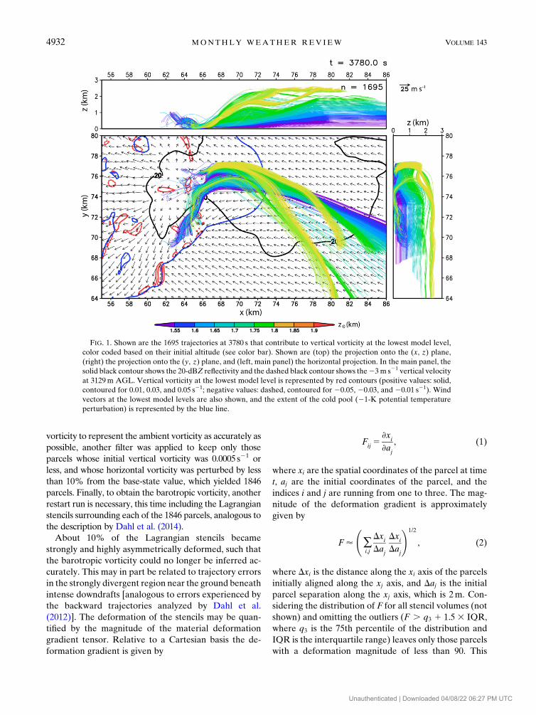
FIG. 1. Shown are the 1695 trajectories at 3780 s that contribute to vertical vorticity at the lowest model level,

color coded based on their initial altitude (see color bar). Shown are (top) the projection onto the (x, z) plane,

(right) the projection onto the (y, z) plane, and (left, main panel) the horizontal projection. In the main panel, the

solid black contour shows the 20-dBZ reflectivity and the dashed black contour shows the23m s21 vertical velocity

at 3129m AGL. Vertical vorticity at the lowest model level is represented by red contours (positive values: solid,

contoured for 0.01, 0.03, and 0.05 s21; negative values: dashed, contoured for 20.05, 20.03, and 20.01 s21). Wind

vectors at the lowest model levels are also shown, and the extent of the cold pool (21-K potential temperature

perturbation) is represented by the blue line.



criterion conveniently filters out those parcels belonging

to a common stencil that strongly diverge at the base of a

downdraft. If only these ‘‘well behaved’’ stencils

(F, 90) are retained, a total of 1695 parcels remains.

For the double-moment simulation, the same initial

conditions and filtering criteria of the trajectories in the

downdraft were used, except that 0:0, z, 0:0005 s21

and 20:3,w, 0m s21. These criteria were chosen to

include those parcels with near-zero positive vertical

vorticity in weak downdrafts (thereby also testing the

robustness of the parcel-selection criteria), while at the

same time keeping the overall number of identified

parcels manageable.3 To identify those parcels that

were sufficiently unperturbed initially, a 5% pertur-

bation of the horizontal vorticity was admitted and the

vertical-vorticity magnitude needed to be less than 531025 s21. These more stringent criteria compared to the

single-moment run were used to reflect the smaller

z threshold stipulated at the downdraft base. Using

again the F, 90 criterion yielded 330 parcels of inter-

est for the simulation with the double-moment micro-

physics scheme.

3. Results

a. Single-moment microphysics simulation

An overview of the storm including the analyzed

trajectories is shown in Fig. 1. The trajectories, as in

previous simulations (e.g., Adlerman et al. 1999; Dahl

et al. 2012, 2014; Markowski and Richardson 2014;

Parker and Dahl 2015), originate from the lowest few

kilometers above the ground. This trajectory sample

includes several parcels that start out near the ground,

but then rise along the left-flank convergence boundary

(Beck andWeiss 2013) and subsequently descend within

the main downdraft north of the mesocyclone. The tra-

jectories reach the lowest model level at different times

[at the time shown, some of the parcels are already rising

in the main updraft near (x, y)5 (63, 70) kmwhile other

parcels are just approaching the lowest model level, e.g.,

near (x, y)5 (67, 76) km].

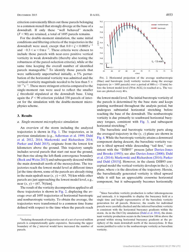
The result of the vorticity decomposition applied to all

these trajectories is shown in Fig. 2, displaying the av-

erage over all 1695 trajectories of horizontal barotropic

and nonbarotropic vorticity. To obtain the average, the

trajectories were transformed to a common time frame

defined with respect to the time when the parcels reach

the lowest model level. The initial barotropic vorticity of

the parcels is determined by the base state and keeps

pointing northward throughout the analysis period, but

undergoes substantial horizontal stretching before

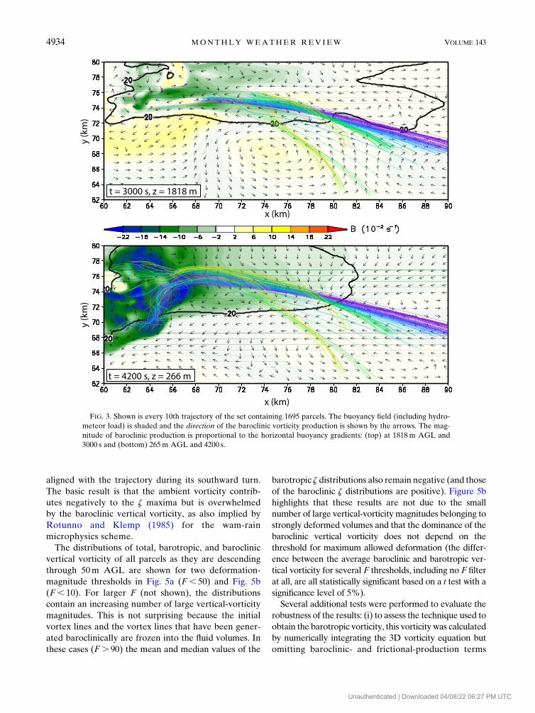
reaching the base of the downdraft. The nonbarotropic

vorticity is due primarily to southward horizontal buoy-

ancy torques, consistent with Fig. 3, and subsequent

horizontal stretching.4

The baroclinic and barotropic vorticity parts along

the averaged trajectory in the (y, z) plane are shown in

Fig. 4.While the barotropic vorticity attains a downward

component during descent, the baroclinic vorticity vec-

tor is tilted upward while descending ‘‘tail first,’’ con-

sistent with the ‘‘DJB93’’ process [after Davies-Jones

and Brooks (1993); see also Davies-Jones (2000); Dahl

et al. (2014); Markowski and Richardson (2014); Parker

and Dahl (2015)]. However, in the classic DJB93 con-

ceptual model the vertical vorticity develops in the (s, z)

plane, where s is the direction of the trajectory. Herein,

the baroclinically generated vorticity is tilted upward

while it still has an appreciable crosswise horizontal

component, but it subsequently becomes horizontally

FIG. 2. Horizontal projection of the average nonbarotropic

(blue) and barotropic (red) vorticity vectors along the average

trajectory (n5 1695 parcels) over a period of 800 s (;13min) be-

fore the lowest model level (50m AGL) is reached at t0. The vec-

tors are plotted every 40 s.

3 Isolating thousands of trajectories out of a set of several million

parcels is computationally quite expensive. Increasing the upper

boundary of the z interval would have increased the number of

parcels.

4 Since baroclinic vorticity production is rather inhomogeneous

and unsteady, it is impossible to display the buoyancy field at a

single time and height representative of the baroclinic vorticity

generation for all parcels. However, the results for individual

parcels were carefully checked and the inferred baroclinic vorticity

is consistent with the horizontal buoyancy gradients within the

storm. As in the Del City simulation (Dahl et al. 2014), the domi-

nant vorticity production occurs in the lowest few 100m above the

ground within strong horizontal buoyancy gradients at the pe-

riphery of the main downdraft north of the mesocyclone. It thus

seems justified to refer to the nonbarotropic vorticity as baroclinic

vorticity.



aligned with the trajectory during its southward turn.

The basic result is that the ambient vorticity contrib-

utes negatively to the z maxima but is overwhelmed

by the baroclinic vertical vorticity, as also implied by

Rotunno and Klemp (1985) for the wam-rain

microphysics scheme.

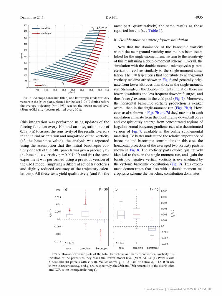
The distributions of total, barotropic, and baroclinic

vertical vorticity of all parcels as they are descending

through 50m AGL are shown for two deformation-

magnitude thresholds in Fig. 5a (F, 50) and Fig. 5b

(F, 10). For larger F (not shown), the distributions

contain an increasing number of large vertical-vorticity

magnitudes. This is not surprising because the initial

vortex lines and the vortex lines that have been gener-

ated baroclinically are frozen into the fluid volumes. In

these cases (F. 90) the mean and median values of the

barotropic z distributions also remain negative (and those

of the baroclinic z distributions are positive). Figure 5b

highlights that these results are not due to the small

number of large vertical-vorticity magnitudes belonging to

strongly deformed volumes and that the dominance of the

baroclinic vertical vorticity does not depend on the

threshold for maximum allowed deformation (the differ-

ence between the average baroclinic and barotropic ver-

tical vorticity for several F thresholds, including no F filter

at all, are all statistically significant based on a t test with a

significance level of 5%).

Several additional tests were performed to evaluate the

robustness of the results: (i) to assess the technique used to

obtain the barotropic vorticity, this vorticity was calculated

by numerically integrating the 3D vorticity equation but

omitting baroclinic- and frictional-production terms

FIG. 3. Shown is every 10th trajectory of the set containing 1695 parcels. The buoyancy field (including hydro-

meteor load) is shaded and the direction of the baroclinic vorticity production is shown by the arrows. The mag-

nitude of baroclinic production is proportional to the horizontal buoyancy gradients: (top) at 1818m AGL and

3000 s and (bottom) 265m AGL and 4200 s.



(this integration was performed using updates of the

forcing function every 10 s and an integration step of

0.1 s); (ii) to assess the sensitivity of the results to errors

in the initial orientation and magnitude of the vorticity

(cf. the base-state value), the analysis was repeated

using the assumption that the initial barotropic vor-

ticity of each of the 3481 parcels was given precisely by

the base-state vorticity h5 0:004 s21; and (iii) the same

experiment was performed using a previous version of

the CM1 model (implying a different set of trajectories

and slightly reduced accuracy of the trajectory calcu-

lations). All these tests yield qualitatively (and for the

most part, quantitatively) the same results as those

reported herein (see Table 1).

b. Double-moment microphysics simulation

Now that the dominance of the baroclinic vorticity

within the near-ground vorticity maxima has been estab-

lished for the single-moment run, we turn to the sensitivity

of this result using a double-moment scheme. Overall, the

simulation with the double-moment microphysics param-

eterization evolves similarly to the single-moment simu-

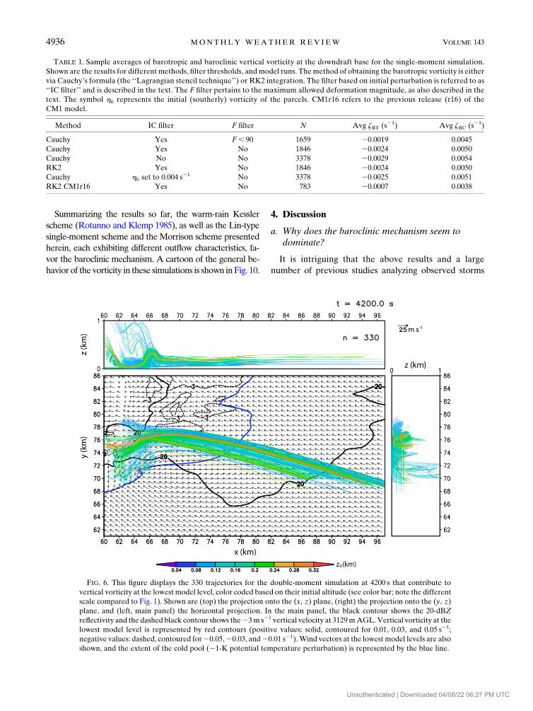
lation. The 330 trajectories that contribute to near-ground

vorticity maxima are shown in Fig. 6 and generally origi-

nate from lower altitudes than those in the single-moment

run. Strikingly, in the double-moment simulation there are

fewer downdrafts and less frequent downdraft surges, and

thus fewer z extrema in the cold pool (Fig. 7). Moreover,

the horizontal baroclinic vorticity production is weaker

overall than in the single-moment run (Figs. 7b,d). How-

ever, as also shown in Figs. 7b and 7d the zmaxima in each

simulation emanate from themost intense downdraft cores

and conspicuously emerge from concentrated regions of

large horizontal buoyancy gradients (see also the animated

version of Fig. 7, available in the online supplemental

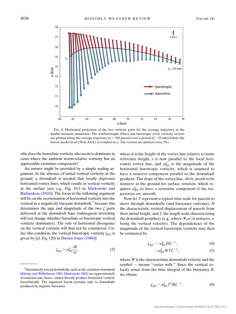
material). To better understand the relative importance of

baroclinic and barotropic contributions in this case, the

horizontal projection of the averaged two vorticity parts is

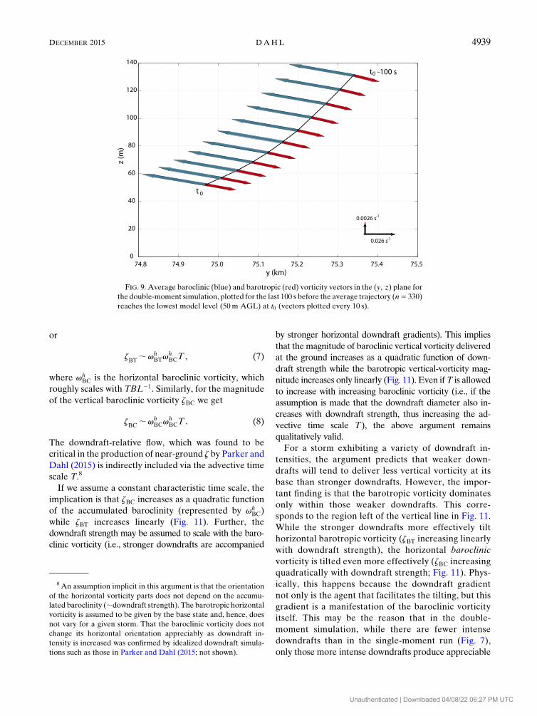
shown in Fig. 8. The vorticity parts evolve qualitatively

identical to those in the single-moment run, and again the

barotropic negative vertical vorticity is overwhelmed by

the cyclonic baroclinic contribution (Fig. 9). This experi-

ment demonstrates that also with a double-moment mi-

crophysics scheme the baroclinic contribution dominates.

FIG. 4. Average baroclinic (blue) and barotropic (red) vorticity

vectors in the (y, z) plane, plotted for the last 210 s (3.5min) before

the average trajectory (n5 1695) reaches the lowest model level

(50m AGL) at t0 (vectors plotted every 10 s).

FIG. 5. Box-and-whisker plots of the total, baroclinic, and barotropic vertical-vorticity dis-

tribution of the parcels as they reach the lowest model level (50m AGL). (a) Parcels with

F, 50 and (b) parcels with F, 10. Values above q3 1 1:5 IQR or below q1 2 1:5 IQR are

shown as red crosses (q1 and q3 are, respectively, the 25th and 75th percentile of the distribution

and IQR is the interquartile range).



Summarizing the results so far, the warm-rain Kessler

scheme (Rotunno and Klemp 1985), as well as the Lin-type

single-moment scheme and the Morrison scheme presented

herein, each exhibiting different outflow characteristics, fa-

vor the baroclinic mechanism. A cartoon of the general be-

havior of the vorticity in these simulations is shown inFig. 10.

4. Discussion

a. Why does the baroclinic mechanism seem todominate?

It is intriguing that the above results and a large

number of previous studies analyzing observed storms

TABLE 1. Sample averages of barotropic and baroclinic vertical vorticity at the downdraft base for the single-moment simulation.

Shown are the results for different methods, filter thresholds, andmodel runs. Themethod of obtaining the barotropic vorticity is either

via Cauchy’s formula (the ‘‘Lagrangian stencil technique’’) or RK2 integration. The filter based on initial perturbation is referred to as

‘‘IC filter’’ and is described in the text. The F filter pertains to the maximum allowed deformation magnitude, as also described in the

text. The symbol h0 represents the initial (southerly) vorticity of the parcels. CM1r16 refers to the previous release (r16) of the

CM1 model.

Method IC filter F filter N Avg zBT (s21) Avg zBC (s21)

Cauchy Yes F, 90 1659 20.0019 0.0045

Cauchy Yes No 1846 20.0024 0.0050

Cauchy No No 3378 20.0029 0.0054

RK2 Yes No 1846 20.0024 0.0050

Cauchy h0 set to 0.004 s21 No 3378 20.0025 0.0051

RK2 CM1r16 Yes No 783 20.0007 0.0038

FIG. 6. This figure displays the 330 trajectories for the double-moment simulation at 4200 s that contribute to

vertical vorticity at the lowest model level, color coded based on their initial altitude (see color bar; note the different

scale compared to Fig. 1). Shown are (top) the projection onto the (x, z) plane, (right) the projection onto the (y, z)

plane, and (left, main panel) the horizontal projection. In the main panel, the black contour shows the 20-dBZ

reflectivity and the dashed black contour shows the23m s21 vertical velocity at 3129mAGL.Vertical vorticity at the

lowest model level is represented by red contours (positive values: solid, contoured for 0.01, 0.03, and 0.05 s21;

negative values: dashed, contoured for20.05,20.03, and20.01 s21).Wind vectors at the lowest model levels are also

shown, and the extent of the cold pool (21-K potential temperature perturbation) is represented by the blue line.



and idealized simulations consistently find that downdraft

production of vertical vorticity near the ground is due

primarily to the baroclinic mechanism.5 This implies that

the barotropic mechanism is ineffective for a wide range

of representations of cloud microphysics ranging from

warm-rain (Rotunno and Klemp 1985; Davies-Jones and

Brooks 1993; Wicker and Wilhelmson 1995; Adlerman

et al. 1999) to Lin-type (Dahl et al. 2014 and this study) to

double-moment (this study) to idealized heat sink

(Markowski andRichardson 2014; Parker andDahl 2015)

parameterizations, as well as observed cases (Markowski

et al. 2008, 2012). It is, thus, tempting to speculate that

there is a fundamental reason that leads to this domi-

nance of baroclinic vorticity.6 The leading-order effect is

most likely that tornadic environments tend to be domi-

nated by streamwise ambient storm-relative vorticity,

implying that in such cases the ambient vorticity does not

contribute to ground-level z as discussed in section 1. But,

FIG. 7. A snapshot of the simulation using (a),(b) the single-moment microphysics scheme and (c),(d) the double-moment microphysics

scheme. (a) Buoyancy (including hydrometeor load; shaded), vertical velocity (22m s21; black contours) at 265mAGL, and positive z at

the lowest model level (contoured for 0.005 and 0.01 s21) at 4500 s. (b) As in (a), but that the shaded field is themagnitude of the buoyancy

torque. (c),(d) As in (a),(b), but for the double-moment simulation and at 4710 s.

5 The author is aware of only one study that suggests that am-

bient vorticity is the dominant contributor to an intense near-

ground vortex in a supercell (Mashiko et al. 2009). However, these

authors calculated parcel histories of only about 5min prior to the

parcels entering the vortex, which makes it rather unlikely that the

initial (barotropic) vorticity corresponded to the ambient vorticity.

6 The basic downdraft processes simulated by Parker and Dahl

(2015) were not changed in important ways when surface friction

was included in their simulations, implying that at least for the

onset of near-ground rotation, surface friction is not the dominant

contributor. This point will be addressed again at the end of this

section.



why does the baroclinic vorticity also seem to dominate in

cases where the ambient storm-relative vorticity has an

appreciable crosswise component?

An answer might be provided by a simple scaling ar-

gument. In the absence of initial vertical vorticity at the

ground, a downdraft is needed that locally depresses

horizontal vortex lines, which results in vertical vorticity

at the surface [see e.g., Fig. 10.3 in Markowski and

Richardson (2010)]. The focus in the following argument

will be on the reorientation of horizontal vorticity into the

vertical in a negatively buoyant downdraft,7 because this

determines the sign and magnitude of the two z parts

delivered at the downdraft base (subsequent stretching

will not change whether baroclinic or barotropic vertical

vorticity dominates). The role of horizontal divergence

on the vertical vorticity will thus not be considered. Un-

der this condition, the vertical barotropic vorticity zBT is

given by [cf. Eq. (20) in Davies-Jones (1984)]

zBT

5vhBT

›h

›s, (3)

where h is the height of the vortex line relative to some

reference height, s is now parallel to the local hori-

zontal vortex line, and vhBT is the magnitude of the

horizontal barotropic vorticity, which is assumed to

have a nonzero component parallel to the downdraft

gradient. The slope of the vortex line, ›h/›s, needs to be

nonzero at the ground for surface rotation, which re-

quires vhBT to have a crosswise component if the tra-

jectories are smooth.

Now let T represent a typical time scale for parcels to

move through downdrafts (and buoyancy extrema), H

the characteristic vertical displacement of parcels from

their initial height, and L the length scale characterizing

the downdraft periphery (e.g., where j$hwj is nonzero,wbeing the vertical velocity). The dependencies of the

magnitude of the vertical barotropic vorticity may then

be estimated by

zBT

; vhBTHL21 , (4)

;vhBTWTL21 , (5)

whereW is the characteristic downdraft velocity and the

symbol ; means ‘‘varies with.’’ Since the vertical ve-

locity arises from the time integral of the buoyancy B,

we obtain

zBT

;vhBTT

2BL21 , (6)

FIG. 8. Horizontal projection of the two vorticity parts for the average trajectory in the

double-moment simulation. The nonbarotropic (blue) and barotropic (red) vorticity vectors

are plotted along the average trajectory (n5 330 parcels over a period of ;25min) before the

lowest model level (50m AGL) is reached at t0. The vectors are plotted every 50 s.

7 Dynamically forced downdrafts, such as the occlusion downdraft

(Klemp and Wilhelmson 1983; Markowski 2002) are approximately

irrotational and, hence, cannot directly produce horizontal vorticity

baroclinically. The argument herein pertains only to downdrafts

produced by negative buoyancy.



or

zBT

;vhBTv

hBCT , (7)

where vhBC is the horizontal baroclinic vorticity, which

roughly scales with TBL21. Similarly, for the magnitude

of the vertical baroclinic vorticity zBC we get

zBC

;vhBCv

hBCT . (8)

The downdraft-relative flow, which was found to be

critical in the production of near-ground z by Parker and

Dahl (2015) is indirectly included via the advective time

scale T.8

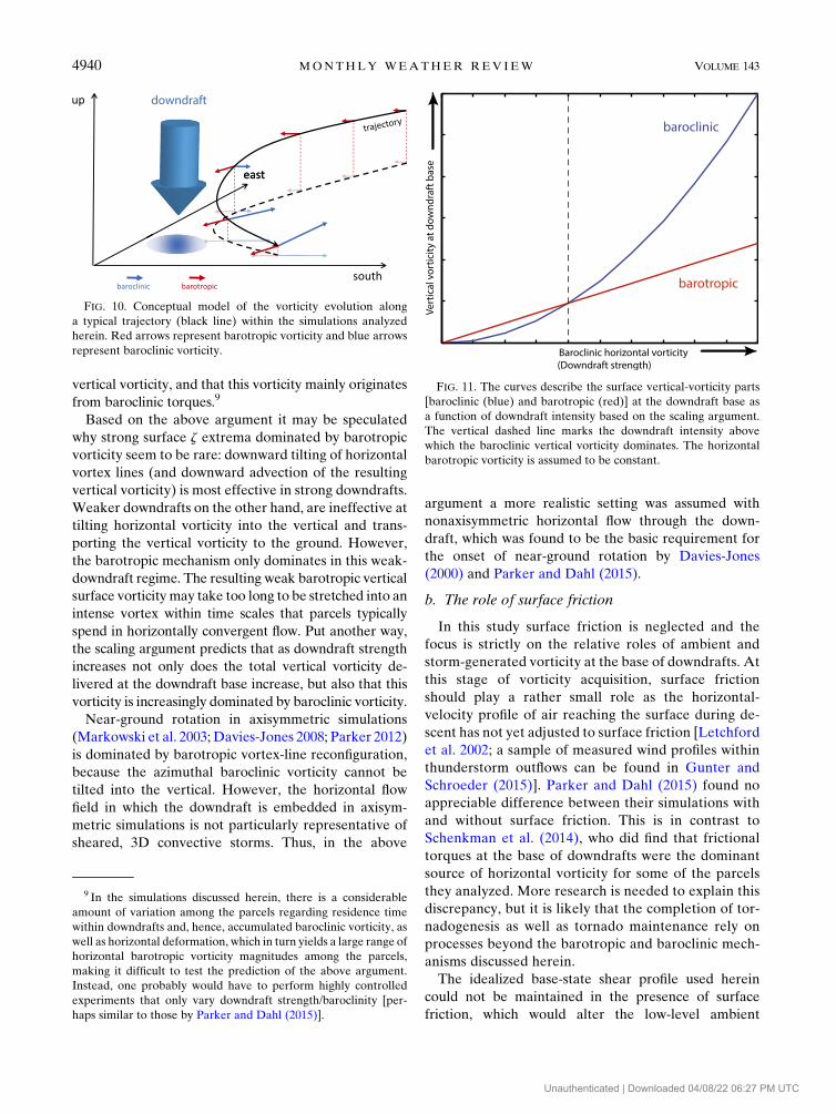
If we assume a constant characteristic time scale, the

implication is that zBC increases as a quadratic function

of the accumulated baroclinity (represented by vhBC)

while zBT increases linearly (Fig. 11). Further, the

downdraft strength may be assumed to scale with the baro-

clinic vorticity (i.e., stronger downdrafts are accompanied

by stronger horizontal downdraft gradients). This implies

that the magnitude of baroclinic vertical vorticity delivered

at the ground increases as a quadratic function of down-

draft strength while the barotropic vertical-vorticity mag-

nitude increases only linearly (Fig. 11). Even ifT is allowed

to increase with increasing baroclinic vorticity (i.e., if the

assumption is made that the downdraft diameter also in-

creases with downdraft strength, thus increasing the ad-

vective time scale T), the above argument remains

qualitatively valid.

For a storm exhibiting a variety of downdraft in-

tensities, the argument predicts that weaker down-

drafts will tend to deliver less vertical vorticity at its

base than stronger downdrafts. However, the impor-

tant finding is that the barotropic vorticity dominates

only within those weaker downdrafts. This corre-

sponds to the region left of the vertical line in Fig. 11.

While the stronger downdrafts more effectively tilt

horizontal barotropic vorticity (zBT increasing linearly

with downdraft strength), the horizontal baroclinic

vorticity is tilted even more effectively (zBC increasing

quadratically with downdraft strength; Fig. 11). Phys-

ically, this happens because the downdraft gradient

not only is the agent that facilitates the tilting, but this

gradient is a manifestation of the baroclinic vorticity

itself. This may be the reason that in the double-

moment simulation, while there are fewer intense

downdrafts than in the single-moment run (Fig. 7),

only those more intense downdrafts produce appreciable

FIG. 9. Average baroclinic (blue) and barotropic (red) vorticity vectors in the (y, z) plane for

the double-moment simulation, plotted for the last 100 s before the average trajectory (n5 330)

reaches the lowest model level (50m AGL) at t0 (vectors plotted every 10 s).

8 An assumption implicit in this argument is that the orientation

of the horizontal vorticity parts does not depend on the accumu-

lated baroclinity (;downdraft strength). The barotropic horizontal

vorticity is assumed to be given by the base state and, hence, does

not vary for a given storm. That the baroclinic vorticity does not

change its horizontal orientation appreciably as downdraft in-

tensity is increased was confirmed by idealized downdraft simula-

tions such as those in Parker and Dahl (2015; not shown).



vertical vorticity, and that this vorticity mainly originates

from baroclinic torques.9

Based on the above argument it may be speculated

why strong surface z extrema dominated by barotropic

vorticity seem to be rare: downward tilting of horizontal

vortex lines (and downward advection of the resulting

vertical vorticity) is most effective in strong downdrafts.

Weaker downdrafts on the other hand, are ineffective at

tilting horizontal vorticity into the vertical and trans-

porting the vertical vorticity to the ground. However,

the barotropic mechanism only dominates in this weak-

downdraft regime. The resulting weak barotropic vertical

surface vorticity may take too long to be stretched into an

intense vortex within time scales that parcels typically

spend in horizontally convergent flow. Put another way,

the scaling argument predicts that as downdraft strength

increases not only does the total vertical vorticity de-

livered at the downdraft base increase, but also that this

vorticity is increasingly dominated by baroclinic vorticity.

Near-ground rotation in axisymmetric simulations

(Markowski et al. 2003; Davies-Jones 2008; Parker 2012)

is dominated by barotropic vortex-line reconfiguration,

because the azimuthal baroclinic vorticity cannot be

tilted into the vertical. However, the horizontal flow

field in which the downdraft is embedded in axisym-

metric simulations is not particularly representative of

sheared, 3D convective storms. Thus, in the above

argument a more realistic setting was assumed with

nonaxisymmetric horizontal flow through the down-

draft, which was found to be the basic requirement for

the onset of near-ground rotation by Davies-Jones

(2000) and Parker and Dahl (2015).

b. The role of surface friction

In this study surface friction is neglected and the

focus is strictly on the relative roles of ambient and

storm-generated vorticity at the base of downdrafts. At

this stage of vorticity acquisition, surface friction

should play a rather small role as the horizontal-

velocity profile of air reaching the surface during de-

scent has not yet adjusted to surface friction [Letchford

et al. 2002; a sample of measured wind profiles within

thunderstorm outflows can be found in Gunter and

Schroeder (2015)]. Parker and Dahl (2015) found no

appreciable difference between their simulations with

and without surface friction. This is in contrast to

Schenkman et al. (2014), who did find that frictional

torques at the base of downdrafts were the dominant

source of horizontal vorticity for some of the parcels

they analyzed. More research is needed to explain this

discrepancy, but it is likely that the completion of tor-

nadogenesis as well as tornado maintenance rely on

processes beyond the barotropic and baroclinic mech-

anisms discussed herein.

The idealized base-state shear profile used herein

could not be maintained in the presence of surface

friction, which would alter the low-level ambient

FIG. 10. Conceptual model of the vorticity evolution along

a typical trajectory (black line) within the simulations analyzed

herein. Red arrows represent barotropic vorticity and blue arrows

represent baroclinic vorticity.

FIG. 11. The curves describe the surface vertical-vorticity parts

[baroclinic (blue) and barotropic (red)] at the downdraft base as

a function of downdraft intensity based on the scaling argument.

The vertical dashed line marks the downdraft intensity above

which the baroclinic vertical vorticity dominates. The horizontal

barotropic vorticity is assumed to be constant.

9 In the simulations discussed herein, there is a considerable

amount of variation among the parcels regarding residence time

within downdrafts and, hence, accumulated baroclinic vorticity, as

well as horizontal deformation, which in turn yields a large range of

horizontal barotropic vorticity magnitudes among the parcels,

making it difficult to test the prediction of the above argument.

Instead, one probably would have to perform highly controlled

experiments that only vary downdraft strength/baroclinity [per-

haps similar to those by Parker and Dahl (2015)].



vorticity. The orientation and perhaps the magnitude

of the barotropic vorticity of near-ground parcels riding

up the left-flank boundary would thus be expected to

vary from the results presented herein. The explicit ef-

fect of surface friction in the context of vorticity de-

composition is left for future research.

5. Conclusions

In this study the relative importance of ambient

crosswise (barotropic) vorticity and storm-generated

(baroclinic) vorticity in producing vertical-vorticity

maxima at the base of downdrafts in supercells was in-

vestigated. The goal was to analyze how robust the baro-

clinic mechanism is. Two supercells in unidirectional

shear were simulated, using a single-moment and a

double-moment microphysics parameterization, respec-

tively. A large number of forward trajectories that con-

tribute to cyclonic vorticity at the base of downdrafts was

analyzed for a time period of about 30min and the vor-

ticity was decomposed into barotropic and baroclinic

parts. Independent of themicrophysics parameterization,

the barotropic vorticity remains weaker than the baro-

clinic vorticity and is tilted downward within downdrafts,

while the baroclinic vorticity has a much larger magni-

tude and is tilted upward.

The observation based on this study and previous

work that the dominance of the baroclinic mechanism

seems rather insensitive to the microphysics parame-

terizations (and the shear profiles) may be related to the

following factors: (i) in cases with streamwise ambient

vorticity, the barotropic contribution to near-ground

rotation is small because streamwise vorticity becomes

horizontal along trajectories near the surface; and (ii) in

cases with crosswise ambient vorticity, a scaling argu-

ment predicts that the baroclinic vertical vorticity be-

comes increasingly dominant as downdraft strength

increases. That is, the imported barotropic vorticity

tends to be overwhelmed by baroclinic vorticity except

in the weakest downdrafts, which, however, do not yield

much vertical vorticity altogether at their base. This

mostly barotropic vorticity may be too weak to be con-

centrated effectively by horizontal convergence.

Acknowledgments. I would like to thank Drs. Matt

Parker, Paul Markowski, Lou Wicker, George Bryan,

Yvette Richardson, Bob Davies-Jones, Dan Dawson,

Marcus Büker, and Scott Gunter for insightful discus-

sions. George Bryan is gratefully acknowledged for

maintaining the CM1 model and for implementing the

Lagrange polynomials in the parcel interpolation rou-

tine. I also thank the students in the Atmospheric Sci-

ence Group at TTU for comments on an early draft of

the manuscript. Reviews by Drs. Rich Rotunno, Alex

Schenkman, and an anonymous reviewer contributed

insightful comments that led to additional analysis and

improved the overall presentation.

REFERENCES

Adlerman, E. J., K. K. Droegemeier, and R. P. Davies-Jones, 1999:

A numerical simulation of cyclic mesocyclogenesis. J. Atmos.

Sci., 56, 2045–2069, doi:10.1175/1520-0469(1999)056,2045:

ANSOCM.2.0.CO;2.

Beck, J., and C.Weiss, 2013:An assessment of low-level baroclinity

and vorticity within a simulated supercell. Mon. Wea. Rev.,

141, 649–669, doi:10.1175/MWR-D-11-00115.1.

Bryan, G. H., and J. M. Fritsch, 2002: A benchmark simulation

for moist nonhydrostatic numerical models. Mon. Wea. Rev.,

130, 2917–2928, doi:10.1175/1520-0493(2002)130,2917:

ABSFMN.2.0.CO;2.

Dahl, J. M. L., M. D. Parker, and L. J. Wicker, 2012: Uncertainties

in trajectory calculations within near-surface mesocyclones

of simulated supercells. Mon. Wea. Rev., 140, 2959–2966,

doi:10.1175/MWR-D-12-00131.1.

——, ——, and ——, 2014: Imported and storm-generated near-

ground vertical vorticity in a simulated supercell. J. Atmos.

Sci., 71, 3027–3051, doi:10.1175/JAS-D-13-0123.1.

Davies-Jones, R. P., 1982: Observational and theoretical aspects of

tornadogenesis. Intense Atmospheric Vortices, L. Bengtsson

and J. Lighthill, Eds., Springer, 175–189.

——, 1984: Streamwise vorticity: The origin of updraft rotation in

supercell storms. J. Atmos. Sci., 41, 2991–3006, doi:10.1175/

1520-0469(1984)041,2991:SVTOOU.2.0.CO;2.

——, 2000:ALagrangianmodel for baroclinic genesis ofmesoscale

vortices. Part I: Theory. J. Atmos. Sci., 57, 715–736,

doi:10.1175/1520-0469(2000)057,0715:ALMFBG.2.0.CO;2.

——, 2008: Can a descending rain curtain in a supercell instigate

tornadogenesis barotropically? J. Atmos. Sci., 65, 2469–2497,

doi:10.1175/2007JAS2516.1.

——, and H. E. Brooks, 1993: Mesocyclogenesis from a theoretical

perspective.The Tornado: Its Structure, Dynamics, Prediction,

and Hazards, Geophys. Monogr., Vol. 79, Amer. Geophys.

Union, 105–114.

——, and P. Markowski, 2013: Lifting of ambient air by density

currents in sheared environments. J. Atmos. Sci., 70, 1204–1215,

doi:10.1175/JAS-D-12-0149.1.

——, R. J. Trapp, and H. B. Bluestein, 2001: Tornadoes and tor-

nadic storms. Severe Convective Storms, Meteor. Monogr.,

No. 50, Amer. Meteor. Soc., 167–221.

Dawson, D. T., X. Ming, J. Milbrandt, and M. K. Yau, 2010:

Comparison of evaporation and cold pool development be-

tween single-moment and multimoment bulk microphysics

schemes in idealized simulations of tornadic thunder-

storms. Mon. Wea. Rev., 138, 1152–1170, doi:10.1175/

2009MWR2956.1.

Gilmore, M., J. Straka, and E. Rasmussen, 2004: Precipitation

and evolution sensitivity in simulated deep convective storms:

Comparisons between liquid-only and simple ice and liquid

phase microphysics. Mon. Wea. Rev., 132, 1897–1916,

doi:10.1175/1520-0493(2004)132,1897:PAESIS.2.0.CO;2.

Gunter, W. S., and J. L. Schroeder, 2015: High-resolution full-scale

measurements of thunderstorm outflow winds. J. Wind Eng.

Ind. Aerodyn., 138, 13–26, doi:10.1016/j.jweia.2014.12.005.

Klemp, J. B., and R. B. Wilhelmson, 1983: A study of the tor-

nadic region within a supercell thunderstorm. J. Atmos.



http://dx.doi.org/10.1175/1520-0469(1999)056<2045:ANSOCM>2.0.CO;2

http://dx.doi.org/10.1175/1520-0469(1999)056<2045:ANSOCM>2.0.CO;2

http://dx.doi.org/10.1175/MWR-D-11-00115.1

http://dx.doi.org/10.1175/1520-0493(2002)130<2917:ABSFMN>2.0.CO;2

http://dx.doi.org/10.1175/1520-0493(2002)130<2917:ABSFMN>2.0.CO;2


http://dx.doi.org/10.1175/JAS-D-13-0123.1

http://dx.doi.org/10.1175/1520-0469(1984)041<2991:SVTOOU>2.0.CO;2

http://dx.doi.org/10.1175/1520-0469(1984)041<2991:SVTOOU>2.0.CO;2

http://dx.doi.org/10.1175/1520-0469(2000)057<0715:ALMFBG>2.0.CO;2

http://dx.doi.org/10.1175/2007JAS2516.1


http://dx.doi.org/10.1175/2009MWR2956.1


http://dx.doi.org/10.1175/1520-0493(2004)132<1897:PAESIS>2.0.CO;2

http://dx.doi.org/10.1016/j.jweia.2014.12.005

Sci., 40, 359–377, doi:10.1175/1520-0469(1983)040,0359:

ASOTTR.2.0.CO;2.

Letchford, C.W., C.Mans, andM. T. Chay, 2002: Thunderstorms—

Their importance in wind engineering (a case for the next

generation wind tunnel). J. Wind Eng. Ind. Aerodyn., 90,

1415–1433, doi:10.1016/S0167-6105(02)00262-3.

Loftus, A. M., D. B. Weber, and C. A. Doswell III, 2008: Param-

eterized mesoscale forcing mechanisms for initiating numeri-

cally simulated isolated multicellular convection. Mon. Wea.

Rev., 136, 2408–2421, doi:10.1175/2007MWR2133.1.

Markowski, P. M., 2002: Hook echoes and rear-flank downdrafts:

A review. Mon. Wea. Rev., 130, 852–876, doi:10.1175/

1520-0493(2002)130,0852:HEARFD.2.0.CO;2.

——, and Y. P. Richardson, 2010: Mesoscale Meteorology in Mid-

latitudes. Wiley-Blackwell, 430 pp.

——, and ——, 2014: The influence of environmental low-level

shear and cold pools on tornadogenesis: Insights from ideal-

ized simulations. J. Atmos. Sci., 71, 243–275, doi:10.1175/

JAS-D-13-0159.1.

——, J. M. Straka, and E. N. Rasmussen, 2003: Tornadogenesis

resulting from the transport of circulation by a downdraft:

Idealized numerical simulations. J. Atmos. Sci., 60, 795–823,

doi:10.1175/1520-0469(2003)060,0795:TRFTTO.2.0.CO;2.

——, Y. Richardson, E. Rasmussen, J. Straka, R. P. Davies-Jones,

and R. J. Trapp, 2008: Vortex lines within low-level mesocy-

clones obtained from pseudo-dual-Doppler radar observa-

tions. Mon. Wea. Rev., 136, 3513–3535, doi:10.1175/

2008MWR2315.1.

——, and Coauthors, 2012: The pretornadic phase of the Goshen

County, Wyoming, supercell of 5 June 2009 intercepted by

VORTEX2. Part II: Intensification of low-level rotation.Mon.

Wea. Rev., 140, 2916–2938, doi:10.1175/MWR-D-11-00337.1.

——, Y. Richardson, and G. Bryan, 2014: The origins of vortex

sheets in a simulated supercell thunderstorm.Mon. Wea. Rev.,

142, 3944–3954, doi:10.1175/MWR-D-14-00162.1.

Mashiko, W., H. Niino, and T. Kato, 2009: Numerical simulation of

tornadogenesis in an outer-rainband minisupercell of Ty-

phoon Shanshan on 17 September 2006.Mon. Wea. Rev., 137,

4238–4260, doi:10.1175/2009MWR2959.1.

Morrison, H., G. Thompson, and V. Tatarskii, 2009: Impact of

cloud microphysics on the development of trailing stratiform

precipitation in a simulated squall line: Comparison of one-

and two-moment schemes. Mon. Wea. Rev., 137, 991–1007,doi:10.1175/2008MWR2556.1.

Parker, M. D., 2012: Impacts of lapse rates on low-level rotation in

idealized storms. J. Atmos. Sci., 69, 538–559, doi:10.1175/

JAS-D-11-058.1.

——, and J. M. L. Dahl, 2015: Production of near-surface vertical

vorticity by idealized downdrafts.Mon. Wea. Rev., 143, 2795–

2816, doi:10.1175/MWR-D-14-00310.1.

Rotunno, R., and J. Klemp, 1985: On the rotation and propa-

gation of simulated supercell thunderstorms. J. Atmos.

Sci., 42, 271–292, doi:10.1175/1520-0469(1985)042,0271:

OTRAPO.2.0.CO;2.

Schenkman, A. D., M. Xue, and M. Hu, 2014: Tornadogenesis in a

high-resolution simulation of the 8 May 2003 Oklahoma City

supercell. J. Atmos. Sci., 71, 130–154, doi:10.1175/

JAS-D-13-073.1.

Walko, R. L., 1993: Tornado spin-up beneath a convective cell:

Required basic structure of the near-field boundary layer winds.

The Tornado: Its Structure, Dynamics, Prediction, andHazards,

Geophys. Monogr., Vol. 79, Amer. Geophys. Union, 89–95.

Weisman, M., and J. Klemp, 1982: The dependence of numerically

simulated convective storms on vertical wind shear and

buoyancy. Mon. Wea. Rev., 110, 504–520, doi:10.1175/

1520-0493(1982)110,0504:TDONSC.2.0.CO;2.

Wicker, L. J., and R. B. Wilhelmson, 1995: Simulation and analysis

of tornado development and decay within a three-dimensional

supercell thunderstorm. J. Atmos. Sci., 52, 2675–2703,

doi:10.1175/1520-0469(1995)052,2675:SAAOTD.2.0.CO;2.



http://dx.doi.org/10.1175/1520-0469(1983)040<0359:ASOTTR>2.0.CO;2

http://dx.doi.org/10.1175/1520-0469(1983)040<0359:ASOTTR>2.0.CO;2

http://dx.doi.org/10.1016/S0167-6105(02)00262-3


http://dx.doi.org/10.1175/1520-0493(2002)130<0852:HEARFD>2.0.CO;2

http://dx.doi.org/10.1175/1520-0493(2002)130<0852:HEARFD>2.0.CO;2



http://dx.doi.org/10.1175/1520-0469(2003)060<0795:TRFTTO>2.0.CO;2










http://dx.doi.org/10.1175/1520-0469(1985)042<0271:OTRAPO>2.0.CO;2

http://dx.doi.org/10.1175/1520-0469(1985)042<0271:OTRAPO>2.0.CO;2



http://dx.doi.org/10.1175/1520-0493(1982)110<0504:TDONSC>2.0.CO;2

http://dx.doi.org/10.1175/1520-0493(1982)110<0504:TDONSC>2.0.CO;2

http://dx.doi.org/10.1175/1520-0469(1995)052<2675:SAAOTD>2.0.CO;2

Documents

Near-Ground Rotation in Simulated Supercells: On the