Near-Miscible CO2 Application to Improve Oil Recovery

By

Ly Huong Bui

Submitted to the graduate degree program in Chemical and Petroleum Engineering and the

Graduate Faculty of the University of Kansas in partial fulfillment of the requirement for

the degree of Master of Science

Committee: ____________________________

G. Paul Willhite

___________________________

Jyun Syung Tsau

___________________________

Aaron M. Scurto

Date defended: __________________________

i

Thesis Committee for Ly Huong Bui certifies

that this is the approved version of the following thesis

Near-Miscible CO2 Application to Improve Oil Recovery

Committee: ____________________________

G. Paul Willhite

___________________________

Jyun Syung Tsau

___________________________

Aaron M. Scurto

Date approved: __________________________

ii

ABSTRACT

Carbon dioxide (CO2) injection for enhanced oil recovery is a proven technology. CO2

injection is normally operated at a pressure above the minimum miscibility pressure

(MMP), which is determined by crude oil composition and reservoir conditions. This is the

lowest pressure at which the injected CO2 becomes dynamically miscible with the crude oil

remaining in the reservoir. However, many reservoirs are located at depths or under

geologic conditions such that they must operate at pressures below the MMP. When CO2 is

injected at below the MMP, displacement efficiency decreases as a result of the loss of

miscibility. CO2 injection is usually not considered as an enhanced oil recovery process in

these reservoirs. Near miscible displacement generally refers to the process that occurs at

pressures slightly below the MMP, but the actual pressure range has never been clearly

defined.

The objectives of this study were to investigate the feasibility of near-miscible CO2

application and improve our understanding of the mechanisms of near-miscible CO2

flooding by conducting appropriate experimental work and reservoir simulation. The

pressure range of interest was from 0.8 MMP to MMP in our study. The Arbuckle formation

of Kansas was used as an example to demonstrate our approach to evaluate CO2 flooding at

near-miscible conditions. The suite of laboratory experiments used to evaluate the

feasibility of operating at pressures below MMP for Arbuckle reservoirs included phase

behavior studies, core flow tests and phase behavior model construction using CMG

software package.

iii

Phase behavior studies were carried out to characterize the near miscible conditions. Slim

tube displacements and swelling/extraction tests were performed to identify the near

miscible range and the mass transfer mechanisms which were responsible for the oil

recovery within this range. A phase behavior model was constructed and well-tuned to

simulate oil properties, CO2/crude oil interactions and slim tube results. Core flow tests

were conducted to evaluate the oil recovery efficiency in the near miscible range.

Initial laboratory works indicated that miscibility was not achievable, however at least

65% to 80% of the waterflood residual oil for dolomite cores and lesser from 45% to 60 %

for sandstone core in the near-miscible region was observed. The principal oil recovery

mechanism in the near-miscible range appeared to be extraction/vaporization of

hydrocarbon components from crude oil into the CO2 rich vapor phase, coupled with

enhanced mobility control due to the reduction of oil viscosity. This suggested that

application of carbon dioxide in the field would require injection and recycling of large

volumes of carbon dioxide. Further study is needed to determine if such a process is

economically feasible. However the prospect of recovering up to 1 billion barrels of oil from

Arbuckle reservoirs offers significant economic potential.

iv

TABLE OF CONTENTS

ABSTRACT ................................................................................................................................................ II

TABLE OF CONTENTS .......................................................................................................................... IV

LIST OF TABLES ..................................................................................................................................... XI

NOMENCLATURE ................................................................................................................................ XII

ACKNOWLEDGMENTS ...................................................................................................................... XIV

1 INTRODUCTION AND LITERATURE REVIEW ....................................................................... 1

1.1 THE BASICS OF CO2 EOR .......................................................................................................................... 4

1.1.1 CO2 Properties ......................................................................................................................................... 4

1.1.2 Immiscibility & Miscibility ................................................................................................................. 6

1.1.3 Minimum Miscibility Pressure ......................................................................................................... 8

1.1.4 Mechanisms of Oil Displacement by CO2 ..................................................................................... 9

1.1.5 Mechanisms for CO2 Miscibility with Oil .................................................................................. 11

1.2 MOTIVATIONS BEHIND THIS STUDY ....................................................................................................... 15

1.3 OBJECTIVES OF THE STUDY ..................................................................................................................... 21

2 PHASE BEHAVIOR STUDIES ..................................................................................................... 23

2.1 FLUID PROPERTIES .................................................................................................................................. 23

2.2 SLIM TUBE DISPLACEMENTS ................................................................................................................. 26

2.2.1 Experimental Setup and Specifications .................................................................................... 27

2.2.2 Experimental Procedures ............................................................................................................... 29

2.2.3 Results and Discussions ................................................................................................................... 31

v

2.2.4 Conclusions ........................................................................................................................................... 36

2.3 SWELLING/EXTRACTION TESTS ............................................................................................................ 37

2.3.1 Experimental Setup and specifications .................................................................................... 37

2.3.2 Experimental Procedures ............................................................................................................... 39

2.3.3 Experimental Principles .................................................................................................................. 41

2.3.4 Apparatus Validation ....................................................................................................................... 43

2.3.5 Results and Discussions ................................................................................................................... 44

2.3.5.1 Effect of System Pressure ........................................................................................................................ 44

2.3.5.2 Effect of System Temperature ................................................................................................................. 47

2.3.5.3 Effect of Initial Oil Volume ....................................................................................................................... 50

2.3.6 Conclusions ........................................................................................................................................... 55

2.4 VISCOSITY MEASUREMENTS ................................................................................................................... 55

2.4.1 Principle of Operation ...................................................................................................................... 56

2.4.2 Experimental Setup and Specifications .................................................................................... 57

2.4.3 Experimental Procedures ............................................................................................................... 59

2.4.3.1 Oil Viscosity Measurement Procedure .................................................................................................... 59

2.4.3.2 Oil/CO2 Mixture Viscosity Measurement Procedure ............................................................................. 61

2.4.4 Results and Discussions ................................................................................................................... 62

2.4.5 Conclusions ........................................................................................................................................... 63

2.5 PHASE BEHAVIOR MODEL ...................................................................................................................... 63

2.5.1 Phase Behavior Modeling using WINPROP ............................................................................ 65

2.5.2 Equation of State Characterization ........................................................................................... 68

2.5.3 Slim Tube Modeling using GEM ................................................................................................... 70

3 CORE FLOW TESTS ..................................................................................................................... 76

vi

3.1 CORES ........................................................................................................................................................ 76

3.2 FLUIDS ....................................................................................................................................................... 79

3.3 EQUIPMENTS AND PROCEDURES ........................................................................................................... 79

3.3.1 Core Characterization ..................................................................................................................... 79

3.3.1.1 Pore Volume Measurements .................................................................................................................... 80

3.3.1.1.1 Gravimetric Method ............................................................................................................................ 80

3.3.1.1.2 Tracer Tests ......................................................................................................................................... 81

3.3.1.2 Permeability Measurements .................................................................................................................... 85

3.3.2 Core Floods ........................................................................................................................................... 86

3.3.2.1 Experimental Setup .................................................................................................................................. 86

3.3.2.2 Experimental Procedures ........................................................................................................................ 88

3.3.2.3 Displacement Rate Selection ................................................................................................................... 88

3.4 RESULTS AND DISCUSSIONS ................................................................................................................... 89

3.4.1 Core Characterization Results ...................................................................................................... 89

3.4.2 Core Floods Results ........................................................................................................................... 89

3.4.2.1 Secondary CO2 Flooding ........................................................................................................................... 89

3.4.2.2 Tertiary CO2 flooding ............................................................................................................................... 91

3.4.2.3 Effect of Water Saturation on Oil Recovery Efficiency ........................................................................... 95

3.5 CONCLUSIONS ........................................................................................................................................... 99

4 CONCLUSIONS & RECOMMENDATIONS ............................................................................ 101

4.1 CONCLUSIONS ......................................................................................................................................... 101

4.2 RECOMMENDATIONS ............................................................................................................................. 102

REFERENCES ....................................................................................................................................... 104

APPENDICES ....................................................................................................................................... 107

vii

LIST OF FIGURES

FIGURE 1-1 GAS INJECTION EOR IN U.S [1] ............................................................................................................. 2

FIGURE 1-2 MISCIBLE CO2 GAS INJECTION EOR IN US [1] ................................................................................... 3

FIGURE 1-3 COMPARISON OF CO2, CH4, N2 DENSITY AT 110OF (REFPROP) .................................................. 5

FIGURE 1-4 COMPARISON OF CO2, CH4, N2 VISCOSITY AT 110OF (REFPROP) ............................................... 6

FIGURE 1-5 MISCIBILITY OF PROPANE (OR LPG) LIQUID AND OIL LIQUID AT RESERVOIR TEMPERATURE AND

PRESSURE CONDITIONS [3] ................................................................................................................................. 7

FIGURE 1-6 IMMISCIBLE TWO-PHASE MIXTURE OF METHANE GAS AND OIL LIQUID AT TYPICAL RESERVOIR

CONDITIONS [3] .................................................................................................................................................... 7

FIGURE 1-7 EFFECT OF TEMPERATURE AND PRESSURE ON CO2 INJECTION DISPLACEMENT MECHANISMS [6]

................................................................................................................................................................................ 9

FIGURE 1-8 ONE DIMENSIONAL SCHEMATIC SHOWING HOW CO2 BECOMES MISCIBLE WITH CRUDE OIL ...... 11

FIGURE 1-9 CONCEPT OF MULTIPLE-CONTACT MISCIBILITY BY VAPORIZATION [3] ......................................... 12

FIGURE 1-10 CONCEPT OF MULTIPLE CONTACT MISCIBILITY BY CONDENSATION [3] ..................................... 14

FIGURE 1-11 OIL PRODUCTION FROM ARBUCKLE FORMATION IN TOTAL KANSAS OIL PRODUCTION ............ 15

FIGURE 1-12 EFFECT OF PRESSURE AND PORE VOLUME INJECTED ON TERTIARY FLOOD OIL RECOVERIES IN

SYSTEM 1: CO2/DECANE/BEREA [7] ........................................................................................................... 17

FIGURE 1-13 EFFECT OF PRESSURE AND PORE VOLUME INJECTED ON TERTIARY OIL RECOVERIES IN SYSTEM

2: CO2/WEST TEXAS CRUDE/MIXED-WET CARBONATE CORE AT 100OF [7] ........................................ 17

FIGURE 1-14 COMPARISON OF RESERVOIR S CO2 COREFLOODS WITH TEXAS CREAM LIMESTONE CORE AND

SLIM-TUBE TESTS [11] ..................................................................................................................................... 19

viii

FIGURE 1-15 COMPARISON OF RESERVOIR H CO2 COREFLOODS WITH TEXAS CREAM LIMESTONE CORE AND

SLIM-TUBE TESTS [11] ..................................................................................................................................... 19

FIGURE 1-16 COMPARISON OF RESERVOIR M CO2 COREFLOODS WITH TEXAS CREAM LIMESTONE CORE AND

SLIM-TUBE TESTS [11] ..................................................................................................................................... 20

FIGURE 1-17 COMPARISON OF HYDROCARBON LEAN GAS SLIM TUBE TESTS AND RESERVOIR A COREFLOODS

[11] ..................................................................................................................................................................... 20

FIGURE 1-18 GENERALIZED RECOVERY RESPONSE TO PRESSURE ....................................................................... 22

FIGURE 2-1 OGALLAH UNIT, TREGO COUNTY, KANSAS ........................................................................................ 24

FIGURE 2-2 GC COMPOSITIONAL ANALYSIS RESULT OF OGALLAH CRUDE OIL ................................................... 25

FIGURE 2-3 SCHEMATIC OF SLIM TUBE SETUP ........................................................................................................ 27

FIGURE 2-4 RESULTS OF DISPLACEMENT TESTS AT 110OF .................................................................................. 31

FIGURE 2-5 RESULTS OF DISPLACEMENT TESTS AT 125OF .................................................................................. 32

FIGURE 2-6 MINIMUM MISCIBILITY PRESSURE DETERMINATIONS AT 110OF AND 125OF ............................. 33

FIGURE 2-7 NEAR MISCIBLE REGION FOR OGALLAH CRUDE OIL AT 110OF ....................................................... 34

FIGURE 2-8 DENSITY PROFILE OF THE EFFLUENT AT 110OF ............................................................................... 35

FIGURE 2-9 DENSITY PROFILE OF THE EFFLUENT AT 125OF ............................................................................... 36

FIGURE 2-10 EXPERIMENTAL SETUP INCLUDE (1) GAS CYLINDER (2) ISCO SYRINGE PUMP (3) FISHER

ISOTEMP CIRCULATOR (4) FISHER ISOTEMP IMMERSION CIRCULATOR (5) WATER BATH (6) HIGH

PRESSURE VIEW CELL (7) MIXING BAR (8) LABORATORY JACK (9) COMPUTER (10) CATHETOMETER

WITH TELESCOPE (11) VACUUM PUMP [13] ................................................................................................. 37

FIGURE 2-11 AN ACTUAL IMAGE OF THE SWELLING/EXTRACTION EXPERIMENTAL SETUP ............................. 39

ix

FIGURE 2-12 COMPARISON OF LIQUID PHASE COMPOSITIONS FOR CO2+ N-DECANE SYSTEM AT 71.10OC

(160OF) WITH LITERATURE DATA () THIS WORK () THIS WORK (∆) NAGARAJAN & ROBINSON JR.

(◊) JENNINGS & SCHUCKER ............................................................................................................................. 44

FIGURE 2-13 CHANGE OF INITIAL OIL VOLUME WITH PRESSURE ........................................................................ 45

FIGURE 2-14 EFFECT OF PRESSURE ON CO2 SOLUBILITY AND SWELLING FACTOR AT 110OF ........................ 46

FIGURE 2-15 EFFECT OF TEMPERATURE ON CO2 SOLUBILITY ............................................................................ 48

FIGURE 2-16 EFFECT OF TEMPERATURE ON SWELLING/ EXTRACTION CURVES .............................................. 48

FIGURE 2-17 DEPENDENCE OF CO2 DENSITY ON TEMPERATURE AND PRESSURE (REFPROP) ................... 50

FIGURE 2-18 EFFECT OF INITIAL OIL VOLUME ON CO2 SOLUBILITY AT 110OF ................................................ 51

FIGURE 2-19 EFFECT OF INITIAL OIL VOLUME ON SWELLING/EXTRACTION CURVE AT 110OF ..................... 51

FIGURE 2-20 COMPUTED P-X DIAGRAM FOR THE FLOUNDER OIL/CO2 SYSTEM AT 233OF [16] .................. 53

FIGURE 2-21 COMPUTED P-X DIAGRAM FOR OGALLAH OIL/ CO2 SYSTEM AT 110OF ..................................... 54

FIGURE 2-22 SCHEMATIC OF HIGH-PRESSURE VISCOSITY MEASUREMENT SETUP ............................................ 57

FIGURE 2-23 AN ACTUAL IMAGE OF THE HIGH-PRESSURE VISCOSITY MEASUREMENT SETUP ......................... 58

FIGURE 2-24 A HIGH PRESSURE GENERATOR ......................................................................................................... 59

FIGURE 2-25 EFFECT OF PRESSURE ON OGALLAH VISCOSITY AT 110OF ........................................................... 62

FIGURE 2-26 EFFECT OF CO2 DISSOLUTION IN CRUDE OIL ON THE VISCOSITY OF OGALLAH FLUID ............... 62

FIGURE 2-27 COMPARISON OF VISCOSITY/DENSITY EXPERIMENTAL DATA AND SIMULATED DATA

BEFORE/AFTER EOS TUNING .......................................................................................................................... 69

FIGURE 2-28 COMPARISON OF SATURATION PRESSURE/SWELLING FACTOR EXPERIMENTAL DATA AND

SIMULATED DATA BEFORE/AFTER EOS TUNING .......................................................................................... 70

FIGURE 2-29 RELATIVE PERMEABILITY CURVE OF OIL-GAS USED IN THE SIMULATION [18] .......................... 72

FIGURE 2-30 COMPARISON OF SIMULATED MMP AND EXPERIMENTAL MMP ................................................ 73

x

FIGURE 2-31 RELATIVE PERMEABILITY CURVE OF OIL-GAS BEFORE AND AFTER ADJUSTED TO MATCH SLIM

TUBE RESULTS .................................................................................................................................................... 74

FIGURE 2-32 COMPARISON OF SIMULATED MMP AND EXPERIMENTAL MMP AFTER TUNING THE RELATIVE

PERMEABILITY CURVE ....................................................................................................................................... 75

FIGURE 3-1. VACUUM AND SATURATION SETUP ..................................................................................................... 78

FIGURE 3-2 EQUAL AREA TECHNIQUE IN CALCULATING PV OF A CORE FROM TRACER TESTS ......................... 82

FIGURE 3-3 SCHEMATIC OF TRACER SETUP ............................................................................................................ 84

FIGURE 3-4 SCHEMATIC OF CORE FLOOD SETUP .................................................................................................... 86

FIGURE 3-5 PERCENT OF OIL RECOVERY @ 6 PV OF CO2 INJECTED IN CORE FLOW TESTS AND PERCENT OF

OIL RECOVERY @ 1.2 PV OF CO2 INJECTED IN SLIM TUBE TESTS AT 110OF ........................................... 90

FIGURE 3-6 PERCENT OF OIL RECOVERY @ 6 PV OF CO2 INJECTED AS A FUNCTION OF PRESSURE FOR BEREA

SANDSTONE A1, BAKER DOLOMITE AND ARBUCKLE DOLOMITE AT 110OF ............................................. 93

FIGURE 3-7 RECOVERY EFFICIENCY OF BEREA SANDSTONES A1 & A2 AT 1100 PSIG & 110OF. ................. 95

FIGURE 3-8 EFFECT OF INITIAL WATER SATURATION ON CO2 FLOOD OIL RECOVERY PERFORMANCE BY

COMPARING SECONDARY AND TERTIARY CO2 FLOODS [7] .......................................................................... 97

FIGURE 3-9 EFFECT OF WATER SATURATION ON OIL RECOVERY EFFICIENCY AT 110OF ................................. 98

FIGURE 3-10 CO2 FLOOD END-POINT PERMEABILITY AS A FUNCTION OF WATER SATURATION AND RESIDUAL

OIL SATURATION IN A MIXED WET CARBONATE [7] ...................................................................................... 99

xi

LIST OF TABLES

TABLE 2.1 PHYSICAL PROPERTIES OF OGALLAH CRUDE OIL AND THE LUMPED HEAVY COMPONENT C36+ . 25

TABLE 2.2 SLIM TUBE PROPERTIES .......................................................................................................................... 28

TABLE 2.3 PHASE EQUILIBRIUM DATA OF CO2/N-DECANE AT 71.1OC .............................................................. 43

TABLE 2.5 ADJUSTMENTS OF EOS PARAMETERS .................................................................................................. 68

TABLE 2.6 MAXIMUM PERCENTAGE ERROR BETWEEN SIMULATED AND EXPERIMENTAL DATA .................... 70

TABLE 2.4 SLIM TUBE MODEL PROPERTIES ............................................................................................................ 71

TABLE 3.1 DENSITY/VISCOSITY OF BRINE AT 86OF/110OF .............................................................................. 79

TABLE 3.2 CORE PROPERTIES ................................................................................................................................... 89

TABLE 3.3 TERTIARY CO2 FLOOD RESULTS IN OGALLAH/BEREA SANDSTONE A1 AT 110OF ....................... 92

TABLE 3.4 TERTIARY CO2 FLOOD RESULTS IN OGALLAH/BEREA SANDSTONE A2 AT 110OF ....................... 92

TABLE 3.5 TERTIARY CO2 FLOOD RESULTS IN OGALLAH/ARBUCKLE DOLOMITE AT 110OF ......................... 92

TABLE 3.6 TERTIARY CO2 FLOOD RESULTS IN OGALLAH/ BAKER DOLOMITE AT 110OF ............................... 92

xii

NOMENCLATURE

Swr Connate water saturation

Sorw Residual oil saturation after waterflooding

Sorm Residual oil saturation after CO2 flooding

Swf Water saturation after CO2 flooding

krg Gas relative permeability

kro Oil relative permeability

Sg Gas saturation

µ Viscosity

Tc Critical temperature

T Temperature

Pc Critical pressure

P Pressure

R Molar gas constant

M Molecular weight

Ωa Equation of state parameter

Ωb Equation of state parameter

ω Accentric factor

dij Binary interaction coefficient

α Rotational coupling coefficient

xCO2 Mole fraction of CO2 in the liquid phase

xiii

MW Molecular Weight

PVT Pressure Volume Temperature

PV Pore volume

HCPV Hydrocarbon pore volume

xiv

ACKNOWLEDGMENTS

First and foremost, I would like to express my sincere gratitude to my advisors, Dr. G. Paul

Willhite and Dr. Jyun-Syung Tsau for their guidance, support and encouragement

throughout my graduate study at University of Kansas. I appreciate their patience to guide

me through and make graduate study an invaluable experience to me.

I would like to extend my appreciation to Dr. Aaron M. Scurto for serving on my thesis

committee and giving me insightful comments.

I would like to give my special thanks to Mr. Scott Ramskill and Dr. Karen Peltier for their

assistance on setting up and maintaining laboratory equipment as well as providing me

necessary laboratory supplies to get my work done.

I would like to thank the faculty and staff members of the University of Kansas Center for

Research’s Tertiary Oil Recovery Project (TORP), especially Dr. Jenn-Tai Liang and Ms.

Mayumi Crider. I would also like to thank other fellow students of the Chemical and

Petroleum Department for their friendship.

I would like to acknowledge Research Partnership to Secure Energy for America (RPSEA)

and the University of Kansas Center for Research’s Tertiary Oil Recovery Project (TORP)

for financial support. I would like to acknowledge Kansas Geological Survey and Carmen

Schmitt, Inc. for providing representative core samples and crude oil samples. I would like

xv

to acknowledge Computer Modeling Group (CMG) for their permission of using the

software.

Finally I want to express the deepest appreciation to my mother and my sister for their love

and support.

1

1 Introduction and Literature Review

Crude oil production can include up to three phases: primary, secondary, and tertiary (or

enhanced) oil recovery. Primary oil recovery, which relies on natural reservoir pressure to

drive the oil to the surface, typically produces 5 to 20 % of the original oil in place (OOIP).

Secondary recovery techniques prolong the field's productive life generally by injecting

water or gas to displace oil to production wells, increasing the oil recovery from 20 to 40%

OOIP. Several tertiary, or enhanced oil recovery (EOR) techniques, which have been

attempted with the goal of ultimately recovering/producing 30 to 60 % OOIP and found to

be commercially successful to varying degrees, could be categorized mainly as thermal

recovery, gas injection and chemical injection.

Gas injection involves injecting natural gas, nitrogen or carbon dioxide (CO2) into the

reservoir. The gases can either expand and push oil through the reservoir, or dissolve in the

oil, decreasing its viscosity and facilitating oil flow to the wellbore. While other EOR

methods decline over the years, gas injection increased from 18% in 1984 to about 48% in

2008, proving to be the most popular method in the U.S. The percentage of gas injection

share in total EOR production in the U.S is depicted in Figure 1.1.

2

Figure 1-1 Gas injection EOR in U.S [1]

CO2 injection for secondary and tertiary oil recovery is the primary gas injection method.

Miscible CO2 displacement offers the greatest oil recovery potential, but it can only be

achieved at a pressure greater than a certain minimum referred to as the minimum

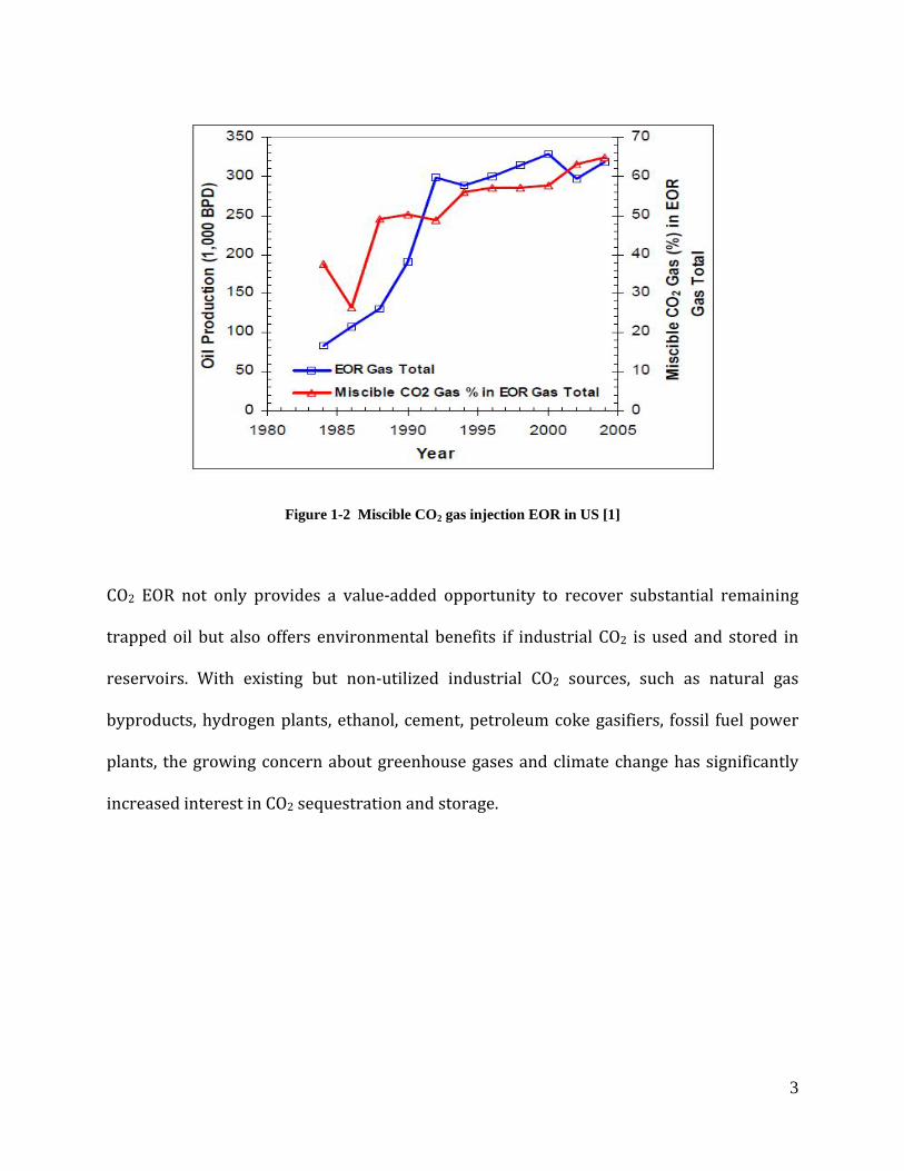
miscibility pressure. In a study of EOR developments and their future potential in the U.S,

Stosur et al. [1] concluded that miscible CO2 gas injection was slowly becoming popular and

would continue to grow faster than any other EOR methods. He pointed out that miscible

CO2 gas injection increased from 38% in 1984 to about 65% in 2004.

3

Figure 1-2 Miscible CO2 gas injection EOR in US [1]

CO2 EOR not only provides a value-added opportunity to recover substantial remaining

trapped oil but also offers environmental benefits if industrial CO2 is used and stored in

reservoirs. With existing but non-utilized industrial CO2 sources, such as natural gas

byproducts, hydrogen plants, ethanol, cement, petroleum coke gasifiers, fossil fuel power

plants, the growing concern about greenhouse gases and climate change has significantly

increased interest in CO2 sequestration and storage.

4

1.1 The Basics of CO2 EOR

1.1.1 CO2 Properties

CO2 has numerous characteristics that make it a favorable oil-displacing-agent. One of the

most important characteristics is the pressure at which CO2 becomes miscible with crude

oil is substantially lower than other gases, although there may be exceptions at high

temperature. When miscibility is attained, residual oil saturation is reduced nearly to zero,

which means high oil recoveries and favorable project economics.

High solubility of CO2 in crude oil is another important characteristic. CO2 dissolution in oil

causes the oil to swell and expand out of dead end pores. In addition, viscosity of crude oil

decreases as it becomes saturated with CO2 at increasing pressures, which helps facilitating

flow to the wellbore. The ability of dense-phase CO2 to extract hydrocarbon components

from oil, coupled with the ability of CO2 to dissolve into oil helps establishing dynamic

miscibility.

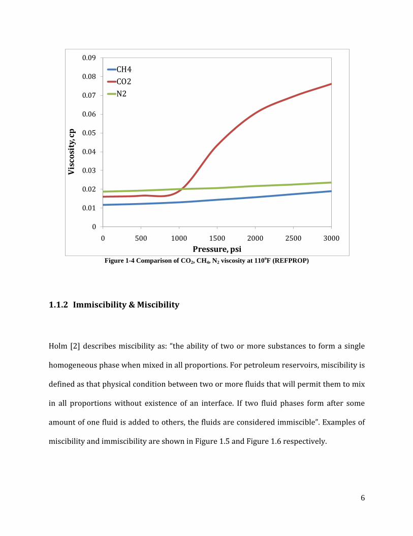
At high pressures, CO2 density has a density close to that of a liquid and is greater than that

of either nitrogen (N2) or methane (CH4), which makes CO2 less prone to gravity

segregation compared with N2 or CH4.

5

Figure 1-3 Comparison of CO2, CH4, N2 density at 110oF (REFPROP)

In addition, at high pressures, viscosity of CO2 is also greater than that of N2 or CH4,

resulting in better mobility control and better sweep efficiency compared with other gases.

0

0.1

0.2

0.3

0.4

0.5

0.6

0.7

0.8

0.9

0 500 1000 1500 2000 2500 3000

Den

sity

, g/c

c

Pressure, psi

CH4CO2N2

6

Figure 1-4 Comparison of CO2, CH4, N2 viscosity at 110oF (REFPROP)

1.1.2 Immiscibility & Miscibility

Holm [2] describes miscibility as: “the ability of two or more substances to form a single

homogeneous phase when mixed in all proportions. For petroleum reservoirs, miscibility is

defined as that physical condition between two or more fluids that will permit them to mix

in all proportions without existence of an interface. If two fluid phases form after some

amount of one fluid is added to others, the fluids are considered immiscible”. Examples of

miscibility and immiscibility are shown in Figure 1.5 and Figure 1.6 respectively.

0

0.01

0.02

0.03

0.04

0.05

0.06

0.07

0.08

0.09

0 500 1000 1500 2000 2500 3000

Vis

cosi

ty, c

p

Pressure, psi

CH4CO2N2

7

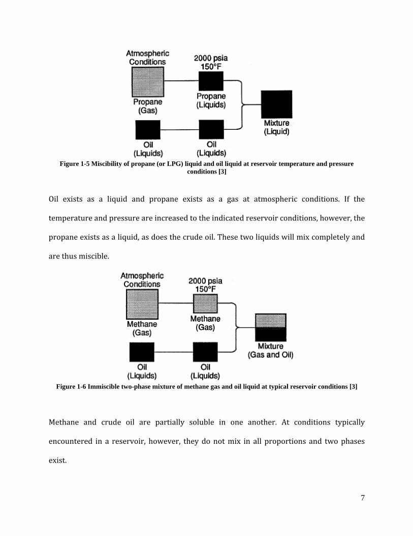
Figure 1-5 Miscibility of propane (or LPG) liquid and oil liquid at reservoir temperature and pressure

conditions [3]

Oil exists as a liquid and propane exists as a gas at atmospheric conditions. If the

temperature and pressure are increased to the indicated reservoir conditions, however, the

propane exists as a liquid, as does the crude oil. These two liquids will mix completely and

are thus miscible.

Figure 1-6 Immiscible two-phase mixture of methane gas and oil liquid at typical reservoir conditions [3]

Methane and crude oil are partially soluble in one another. At conditions typically

encountered in a reservoir, however, they do not mix in all proportions and two phases

exist.

8

1.1.3 Minimum Miscibility Pressure

Miscible recovery of reservoir oil can be achieved by CO2 displacement at a pressure

greater than a certain minimum. This minimum pressure is hereafter called as the CO2

minimum miscibility pressure (MMP). CO2 MMP is an important parameter for screening

and selecting reservoirs for CO2 EOR. For the highest recovery, a candidate reservoir must

be capable of withstanding an average reservoir pressure greater than the CO2 MMP.

MMP depends on crude oil composition and reservoir conditions, and is typically

determined using slim tube tests. There are no fixed criteria for determining miscibility

within slim tube and individual researchers have defined their own criteria to identify slim

tube miscibility. Holm and Josendal [4] defined MMP as the pressure at which 80% of oil in

place was recovered at CO2 breakthrough and more than 94% when gas-oil ratio (GOR)

reaches 40,000 scf/bbl, whereas Metcalfe and Yellig [5] defined MMP as a pressure at

which recovery at 1.2 pore volume gas injected was near the maximum recovery. Others

used the pressure corresponding to the break-over point in the plot of percentage of oil

recovery at 1.2 HCPV of CO2 injected versus pressure as the MMP. In this study, the

pressure at which 90% of original oil in place was recovered at 1.2 HCPV of CO2 injected

was considered MMP.

9

1.1.4 Mechanisms of Oil Displacement by CO2

Mechanisms of CO2 displacing crude oil from porous media rely on the phase behavior of

CO2 /crude oil system, which is strongly dependent on reservoir temperature, pressure and

crude oil composition. Displacement mechanisms fall into one of five regions illustrated in

Figure 1.7. It is important to note that the lines that divide region from region are

generalizations that will vary from oil to oil.

Figure 1-7 Effect of temperature and pressure on CO2 injection displacement mechanisms [6]

In Region I (low pressure applications), CO2 swells the oil, reduces the viscosity of crude oil

and contributes to internal solution gas drive. Swelling of oil is important since the oil left

in the reservoir after flooding is inversely proportional to the swelling factor. Swollen oil

droplets will force water out of pore spaces, creating drainage rather than imbibitions

10

process for water wet system. Drainage oil relative permeability curves are higher than the

imbibitions counterparts, creating a more favorable oil flow environment at any given

saturation conditions. The importance of viscosity reduction was mentioned earlier.

Another mechanism of oil displacement by CO2 in Region I is solution gas drive effect. CO2

goes into the solution with an increase in reservoir pressure, after termination of the

injection phase of a gas flood, gas will come out of solution and continue to drive oil to the

wellbore.

At reservoir pressures higher than those in Region I but lower than Region IV,

supplemental production mechanisms come into play in Region II. In addition to increasing

reservoir pressure, oil swelling, viscosity reduction, hydrocarbons may be vaporized into

the gas phase.

Region III (intermediate pressure, low temperature applications) is very similar to Region

II, except that CO2, rather than vaporize crude oil, extract the crude’s lighter hydrocarbons

forming CO2-rich liquid mixtures. In addition to the potential for reduced total mobility in

the three-phase region, Orr et al (1983) report that CO2-rich liquid phases extract more and

much heavier hydrocarbons than their rich vapor counterparts.

Region IV is the most important region where CO2 vaporizes or extracts a significant

amount of hydrocarbon components from crude oil so rapidly that multiple-contact

miscibility occurs in a very brief time period and over a very short reservoir distance.

11

1.1.5 Mechanisms for CO2 Miscibility with Oil

In general, miscibility between two fluids can be achieved through two mechanisms: first

contact miscibility and multiple contact miscibility.

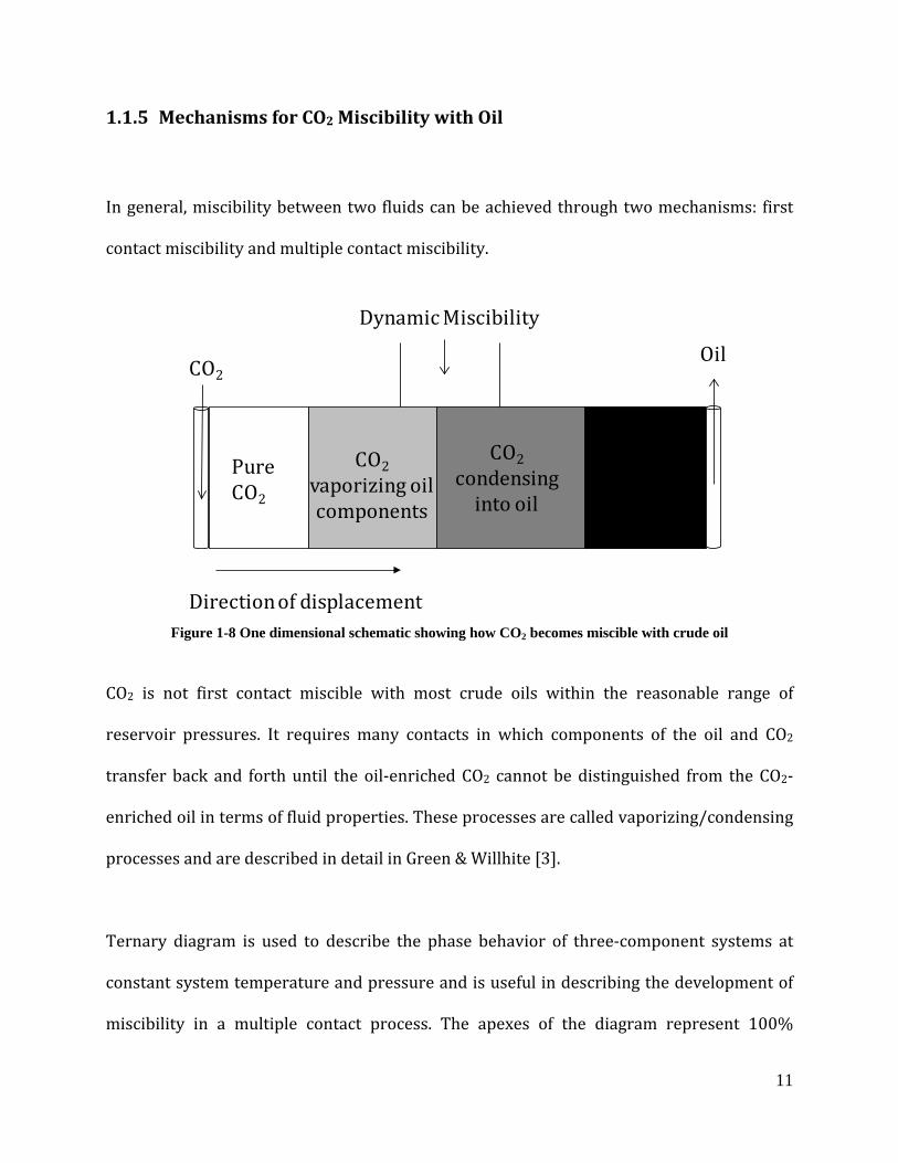
Figure 1-8 One dimensional schematic showing how CO2 becomes miscible with crude oil

CO2 is not first contact miscible with most crude oils within the reasonable range of

reservoir pressures. It requires many contacts in which components of the oil and CO2

transfer back and forth until the oil-enriched CO2 cannot be distinguished from the CO2-

enriched oil in terms of fluid properties. These processes are called vaporizing/condensing

processes and are described in detail in Green & Willhite [3].

Ternary diagram is used to describe the phase behavior of three-component systems at

constant system temperature and pressure and is useful in describing the development of

miscibility in a multiple contact process. The apexes of the diagram represent 100%

Direction of displacement

Original Oil

CO2condensing

into oil

CO2vaporizing oil components

Pure CO2

Dynamic Miscibility

CO2Oil

12

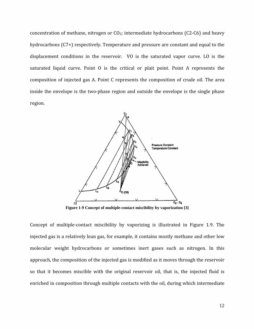
concentration of methane, nitrogen or CO2; intermediate hydrocarbons (C2-C6) and heavy

hydrocarbons (C7+) respectively. Temperature and pressure are constant and equal to the

displacement conditions in the reservoir. VO is the saturated vapor curve. LO is the

saturated liquid curve. Point O is the critical or plait point. Point A represents the

composition of injected gas A. Point C represents the composition of crude oil. The area

inside the envelope is the two-phase region and outside the envelope is the single phase

region.

Figure 1-9 Concept of multiple-contact miscibility by vaporization [3]

Concept of multiple-contact miscibility by vaporizing is illustrated in Figure 1.9. The

injected gas is a relatively lean gas, for example, it contains mostly methane and other low

molecular weight hydrocarbons or sometimes inert gases such as nitrogen. In this

approach, the composition of the injected gas is modified as it moves through the reservoir

so that it becomes miscible with the original reservoir oil, that is, the injected fluid is

enriched in composition through multiple contacts with the oil, during which intermediate

13

components in the oil are vaporized into the injected gas. The process operates

conceptually as follows:

Gas A mixes with Oil C. The resulting composition of the mixture is along AC, say

Point a.

Mixture a is in the two-phase region, therefore, separates into a vapor V1 and a

liquid L1

Vapor V1 moves ahead of Liquid L1 and contacts Oil C. The resulting composition of

the mixture is along Line V1C, say at Point b.

Mixture b separates into Vapor V2 and Liquid L2

The process continues with vapor-phase composition changing along the saturated

vapor curve, V3, V4 etc

Finally, at point e, the vapor becomes miscible with Oil C because the mixing line lies

in the single-phase region.

If miscibility is lost due to reservoir mixing, miscibility is re-developed the same way as

described above. Also, in order for multiple contact miscibility vaporization process to be

successful, the reservoir fluid composition must lie to the right of the critical tie line. If both

fluids lie to the left, vaporization will occur but not in sufficient quantities to develop

miscibility. If the injection fluids and original oil both lie to the right of the critical tie line,

the fluids are miscible on first contact.

14

Figure 1-10 Concept of multiple contact miscibility by condensation [3]

Concept of multiple-contact miscibility by condensation is illustrated in Figure 1.10. The

injected fluid generally contains larger amounts of intermediate molecular weight

hydrocarbons. In this approach, reservoir oil near the injection well is enriched in

composition by contact with the injected fluid since hydrocarbon components are

condensed from the injected fluid into the oil. Under proper conditions, the oil will be

sufficiently modified in composition to become miscible with additional injected fluid.

Conceptually, the process is very similar to vaporizing process, except vapor phase V1, V2

moves ahead, leaving immobile liquid phase L1, L2 etc to mix with additional injected Gas

A.

For multiple contact miscibility by condensation to occur, the injected fluid must be to the

right of the critical tie line. If it is not, condensation of CO2 into crude oil will still occur,

however, miscibility will not be developed.

15

1.2 Motivations behind this study

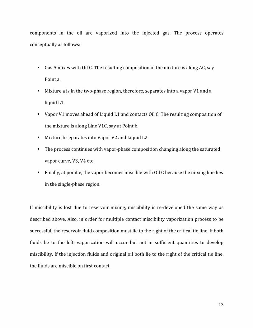
The Arbuckle formation has played an important role in total Kansas oil production. These

Arbuckle reservoirs have produced 2.19 billion barrel of oil by a bottom-water drive

mechanism via an underlying aquifer, representing 36% of total Kansas oil production to

date. Today, more than 90% of wells produce less than 5 barrel of oil per day.

Previous assessments of CO2 miscible flooding in these Arbuckle reservoirs indicate that

miscibility is not achievable at the current reservoir operating pressures. Therefore, the

possibility of operating at pressures below the MMP means that these reservoirs, which

might be otherwise abandoned with substantial remaining oil left in place, could be

considered for CO2 injection.

Arbuckle 36%

Marrow, 3%

Marmaton, 3%

Cherokee, 3%

Simpson, 4% Viola, 5% Lansing-Kansas City,

19%

Mississipian, 16%

Others, 11%

Figure 1-11 Oil production from Arbuckle formation in total Kansas oil production

16

In addition, a lower-pressure process is attractive from both economic and operational

standpoints, including purchasing smaller gas volumes and decreased gas compression

costs.

In general, pressures below MMP are not high enough to vaporize sufficient oil into the CO2

phase or to allow sufficient CO2 to dissolve into the oil so that the two phases to become

miscible. Loss of miscibility results in loss of oil recovery efficiency. Slim tube results

usually show a dramatic loss of recovery at pressures below MMP. To date, however,

conflicting experimental results have led to considerable disagreement in the literature

regarding the feasibility of operating at pressures below MMP.

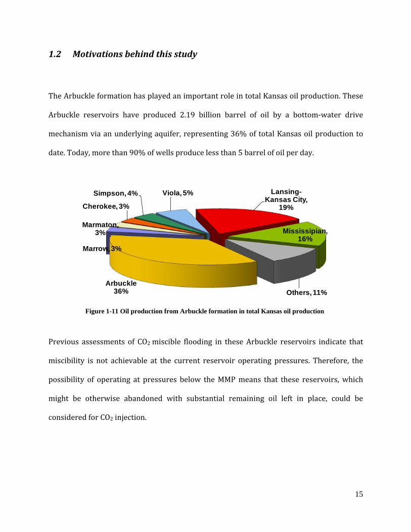
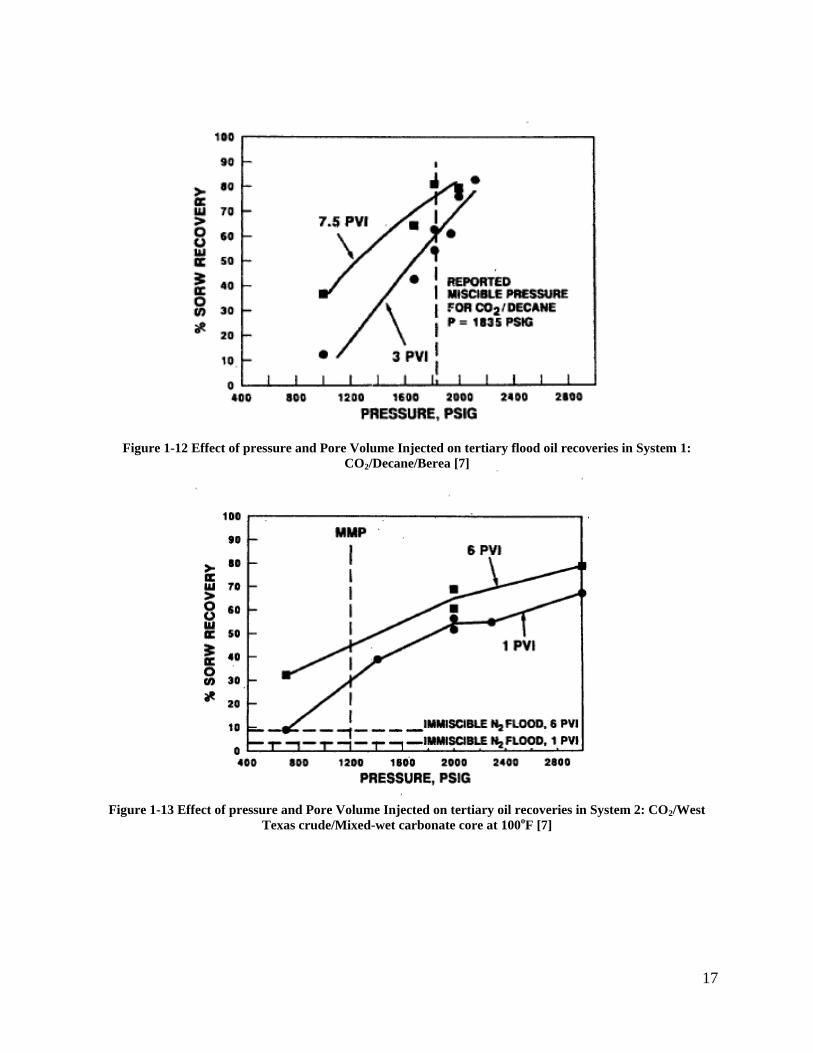
Shyeh-Yung et al. [7] studied the effect of operating pressure by conducting tertiary CO2

displacements on two systems,

System 1-Berea sandstone (strongly water wet)/CO2/decane at 160oF

System 2-San Andres outcrop carbonate (mixed wet)/CO2/ degassed west Texas

separator oil 100oF

Laboratory results presented in Figure 1.12 and Figure 1.13 showed that tertiary CO2 flood

oil recovery decreased linearly as pressure decreased. No dramatic loss of recovery was

observed below the MMP as suggested by slim tube test results.

17

Figure 1-12 Effect of pressure and Pore Volume Injected on tertiary flood oil recoveries in System 1:

CO2/Decane/Berea [7]

Figure 1-13 Effect of pressure and Pore Volume Injected on tertiary oil recoveries in System 2: CO2/West

Texas crude/Mixed-wet carbonate core at 100oF [7]

18

The author attributed the high oil recoveries at pressures below MMP to the possible

improvement of mobility ratio between CO2 and oil, the low IFT displacement and mass

transfer.

Schechter et al. [8] conducted coreflood tests and simulations to examine the possibility of

optimizing the performance of Wellman Unit by reducing CO2 injection pressure, thereby

reducing the volume of CO2. They found that dropping the pressure from above the MMP to

near the MMP or below the MMP did not reduce the efficiency in laboratory coreflooding.

Similarly, a laboratory study on near-miscible CO2 injection in Steelman Reservoir by Dong

et al. [9] showed that the microscopic displacement efficiency improved with operating

pressure in the near-miscible region, but no dramatic change in oil recovery was observed

with a change in operating pressure.

In a recent overview of industrial experience with CO2 injection, Hadlow [10] cited field

data with good recovery at pressures below the CO2 flood MMP in the North Cross and

Dollarhide reservoirs while they were being pressured up.

In another effort by Grigg et al. [11]; however, a rapid decrease in oil recovery was noted as

pressure fell below the MPMP for the CO2 floods conducted at near the CO2 critical

temperature, as slim tube data showed. He also concluded that the concept of hydrocarbon

gas injection is a more feasible concept, and this maybe the case for CO2 injection at

temperatures well above its critical temperature since the hydrocarbon floods did not

19

show a drastic change in oil recovery near the MMP, unlike the CO2 floods. The residual oil

saturations to gasflood as percent of oil after the waterflood are plotted vs. the ratio of the

flood pressure to the slim tube MMP in Figure 1.14 to Figure 1.17.

Figure 1-14 Comparison of Reservoir S CO2 corefloods with Texas Cream limestone core and slim-tube tests

[11]

Figure 1-15 Comparison of Reservoir H CO2 corefloods with Texas Cream limestone core and slim-tube tests

[11]

20

Figure 1-16 Comparison of Reservoir M CO2 corefloods with Texas Cream limestone core and slim-tube tests

[11]

Figure 1-17 Comparison of hydrocarbon lean gas slim tube tests and Reservoir A corefloods [11]

Finally, the most important motivation behind the study is the environmental benefit of

capturing and sequestering CO2 emissions by utilizing an industrial source of CO2. As

significant volumes of injected CO2 used in the displacement stay in the reservoir formation

21

and the produced CO2 from the productions wells is recycled and re-injected into the

reservoir, CO2 emission into the atmosphere and its impact to the environment is very

limit.

1.3 Objectives of the study

The objectives of this study are to (1) investigate the feasibility of near-miscible CO2

application (2) improve our understanding of the mechanisms of near-miscible CO2

flooding by conducting appropriate experimental work and reservoir simulation. The

Arbuckle formation of Kansas is used as an example to demonstrate our approach to

evaluate CO2 flooding at near-miscible conditions. The suite of laboratory experiments used

to evaluate the feasibility of operating at pressures below MMP for Arbuckle reservoirs

includes phase behavior studies, core flow tests and phase behavior model construction

using CMG software package.

The term near miscible is understood as the transition from immiscible to miscible. Near

miscible refers to displacements at pressures slightly below MMP, where the recovery

efficiency is improved over immiscible displacements. Since it is not clearly defined in the

literature, the pressure range of interest in this study is from 0.8 MMP to MMP.

22

Figure 1-18 Generalized recovery response to pressure

0.00.10.20.30.40.50.60.70.80.91.0

0 0.2 0.4 0.6 0.8 1 1.2 1.4

Rec

over

y E

ffic

ien

cy

Relative Miscible Pressure, Pres/MMP

Region 1Miscible

Region 2Immiscible

Region 3Near Miscible

23

2 Phase Behavior Studies

Phase behaviors studies are conducted for several purposes: (1) to characterize the oil/CO2

system (2) to understand the mechanism of oil displacement by CO2 (3) to provide

experimental PVT data to fine-tune the phase behavior model.

Phase behavior studies included slim tube displacements, swelling/extraction tests and

viscosity/density measurements. Slim-tube displacements were conducted to determine

the minimum miscibility pressure for this system and to define the near miscible range.

Swelling/extraction tests were performed to examine the mechanisms of oil recovery in the

near miscible region. Viscosity of oil saturated with CO2 was measured at various

pressures. A phase behavior model based on the Peng-Robinson Equation of State (EOS)

was constructed and well-tuned to characterize the fluid properties and the phase behavior

interaction between CO2 and the oil. Slim tube model was constructed using 1-D

compositional simulation with tuned equation of state. Detail descriptions of phase

behavior studies are presented and discussed in this chapter.

2.1 Fluid Properties

All experiments were performed with centrifuged and filtered Ogallah stock tank oil. The

crude oil was centrifuged at the rate of 20 rpm for at least an hour to separate water, oil

and solid particles. Two layers of glass microfibre filters with the size of 1.6 micron and 1

24

micron were used respectively to filter the crude oil. The location of the unit is shown in

Figure 2.1. The crude oil was obtained from Ogallah Unit, Trego County, Kansas. The unit is

currently operated by Carmen Schmitt, Inc. The unit produces from Arbuckle formation

(3950-4060 ft). Reservoir temperature ranges from 92oF to 130oF with an average

pressure of 111 oF. Active water drives have maintained reservoir pressure at

approximately 1150 psi.

Figure 2-1 Ogallah Unit, Trego County, Kansas

A compositional analysis of the crude oil using Gas Chromatography (GC) technique was

performed by Core Labs and shown in Figure 2.2. % Asphaltenes (heptane insolubles) was

determined approximately 0.93 % based on ASTM D 893-85.

25

Figure 2-2 GC compositional analysis result of Ogallah crude oil

Core Labs also provided physical properties of the oil and the lumped heavy component

C36+, as presented in Table 2.1.

Molecular Weigh, g/mol 228.71 API 33.34 Density @ 14.7 psi & 60oF, g/cc 0.8584 Viscosity @ 14.7 psi & 60oF, cp 13.4 C36+ molecular weight, g/mol 873.24 C36+ density @ 14.7 psi & 60oF, g/cc 0.9978

Table 2.1 Physical properties of Ogallah crude oil and the lumped heavy component C36+

Commercial CO2 of 99.99 % purity was used

0.00

0.02

0.04

0.06

0.08

0.10

0.12

N2 H2S

C2 i-C4i-C5C6 C8 C10C12C14C16C18C20C22C24C26C28C30C32C34C36+

Mol

e fr

acti

on

26

2.2 Slim Tube Displacements

The basis of slim tube tests is that the small-diameter tube filled with an unconsolidated

porous medium serves as an idealized medium for CO2 and crude oil to contact and develop

dynamic miscibility. Non-idealities such as viscous fingering and gravity effect are ignored

because of the large length to diameter ratio in slim tube configuration. Oil recovery is

therefore attributed to the thermodynamic phase behavior of the system. The recovery

performance at different pressures can be used to determine the MMP. Slim tube tests have

not only been used to determine reservoir candidates for miscible processes but also

widely used for fine tuning the reservoir simulator.

In this study, a number of slim tube displacements were conducted for a range of

pressures, holding the temperature constant at the reservoir temperature (110oF-125oF) to

determine the MMP of this system. An oil recovery factor of at least 90% at 1.2 HCPV of CO2

injected is used to define the MMP of the system.

27

2.2.1 Experimental Setup and Specifications

Figure 2-3 Schematic of slim tube setup

Schematic of the slim tube setup is shown in Figure 2.3. Temperature of the system is

controlled and maintained in a Linberg/Blue M oven with Eurotherm temperature

controller. Pressure of the system is controlled and maintained by a back pressure

regulator at the outlet. Back pressure regulator models BPR-50 is a dome-load type, which

controls the upstream back pressure to whatever pressure is applied to the dome. It is

designed to operate using compressed gas in the dome and water, oil, gas in the body. A

Gas

Oil

Electronic BalanceISCO Pump ISCO Pump

PTDPT

DensitometerTest Oil

BPRGas

Oil

Gas

Oil

Electronic BalanceISCO Pump ISCO Pump

PTDPT

DensitometerTest Oil

BPR

28

high pressure bottle of inert gas, such as nitrogen, is required to pressurize the unit. The

back pressure regulator has a working pressure of 5000 psi at 200oF.

Three Valydine pressure transducers are installed to measure pressures at different

locations, such as pressure drop across the slim tube, upstream pressures (CO2/oil

pressure), and downstream pressure (back-pressure regulator pressure). The transducers

have the capability of measuring pressures up to 2500 psi with the accuracy of 0.25% of

their full scale (0-2500 psi).

The injection system consists of two Isco, Inc. 260DM syringe pumps (for CO2/crude oil

transfer and injection at a desired rate) and a transfer cylinder (for crude oil storage). The

capacity of the transfer cylinder is 485 cc. The cylinder can withstand a maximum pressure

of 3000 psi.

The slim tube consists of a coiled 38.29 ft-long stainless steel tube with an ID of 0.24 in.

packed with glass beads. Slim tube properties were evaluated by Rahmatabadi [12] and

listed in Table 2.2.

Length, ft 38.29 O.D, in 0.31 I.D, in 0.24 Porosity 0.37 Bulk volume, cc 347.8 Pore volume, cc 127.76 Permeability, mD 4900 Packing beads No. 2024 Table 2.2 Slim tube properties

29

Density of the effluent is measured continuously by an inline densitometer. The

densitometer consists of two units. The DPRn 422 density transducer measures the

characteristic frequency of vibration. The Anton Paar mPDS 2003V3 Evaluation unit

translates the characteristic frequency of vibration into a density value. The measuring

range is 0-3g/cc within the temperature range of -13oF – 257oF and the pressure range of

0-2900 psi.

Effluent is continuously flashed to atmospheric conditions. The separator gas is connected

to a flow meter. The separator liquid is collected in a graduated cylinder. The graduated

cylinder is placed on an electronic balance which is connected to the data acquisition

system.

2.2.2 Experimental Procedures

At least 2 PV of methylene chloride followed by 2 PV of mineral oil were injected to clean

the slim tube prior to the experiment. The slim tube was then saturated with at least 2 PV

of crude oil at the desired temperature. While the slim tube was being saturated with crude

oil, the system was pressurized gradually to the desired operating pressure using the back

pressure regulator. Upstream pressure changed accordingly to the pressure of the back

pressure regulator as it was set. To prevent pressure from one side of the diaphragm of the

back pressure regulator from becoming significantly higher than the pressure on the other

side and damage the diaphragm, it was necessary to pressurize the system slowly, for

30

example, 0-100 psig, switch off the gas supply valve and wait for the upstream pressure to

catch up with the downstream pressure. Once the desired pressure was reached, the

system was allowed to equilibrate under pressure. Pressure of the CO2 pump was set

slightly above the pressure of the back pressure regulator. Temperature of the pump was

set at temperature of the system. CO2 flow rate was set at a constant of 0.05cc/min. This

corresponds to a Darcy velocity of 8 ft/day.

A log file was created to record the following parameters: temperature of the system,

pressure of the system (back-pressure regulator pressure/downstream pressure),

upstream pressures (CO2/oil pressure), pressure drop across the slim tube, weight of the

separator liquid, and separator gas flow rate. The initial and final volumes of CO2 in the

pump were recorded manually.

The experiment was terminated when at least 1.2 HCPV of CO2 at the temperature and

pressure of the pump were injected. The system was depressurized by venting the dome

load gas slowly. Residual oil in the slim tube was removed by following the same cleaning

procedure as mentioned earlier.

The entire experiment was then repeated several times at different pressures holding other

variables constant.

31

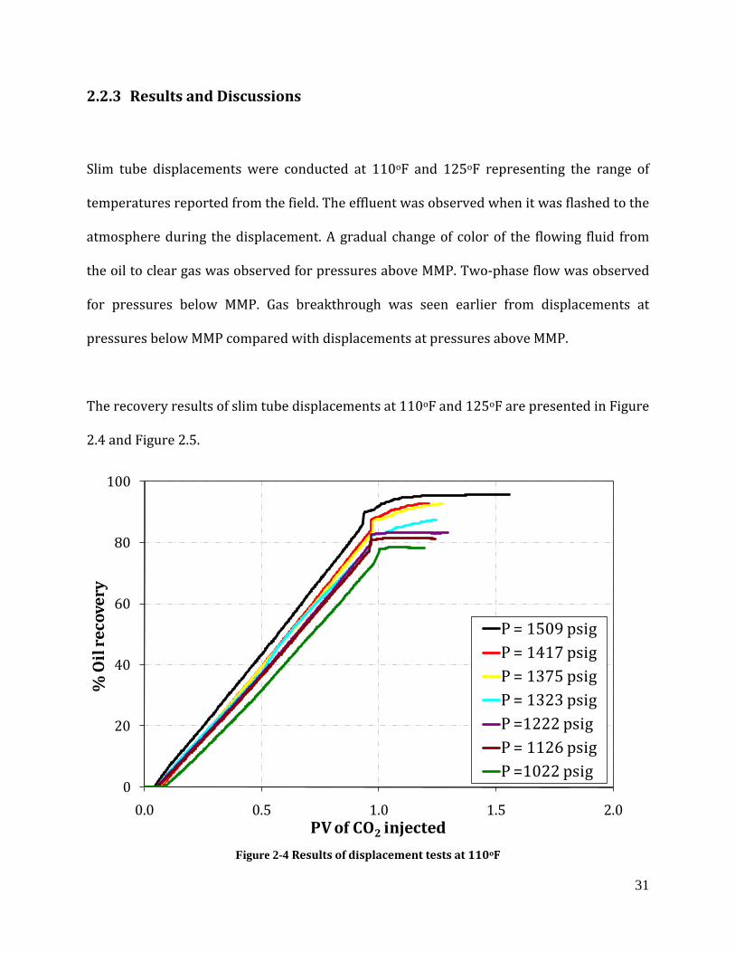
2.2.3 Results and Discussions

Slim tube displacements were conducted at 110oF and 125oF representing the range of

temperatures reported from the field. The effluent was observed when it was flashed to the

atmosphere during the displacement. A gradual change of color of the flowing fluid from

the oil to clear gas was observed for pressures above MMP. Two-phase flow was observed

for pressures below MMP. Gas breakthrough was seen earlier from displacements at

pressures below MMP compared with displacements at pressures above MMP.

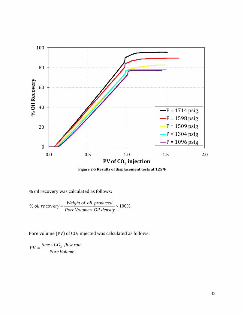
The recovery results of slim tube displacements at 110oF and 125oF are presented in Figure

2.4 and Figure 2.5.

Figure 2-4 Results of displacement tests at 110oF

0

20

40

60

80

100

0.0 0.5 1.0 1.5 2.0

% O

il r

ecov

ery

PV of CO2 injected

P = 1509 psigP = 1417 psigP = 1375 psigP = 1323 psigP =1222 psigP = 1126 psigP =1022 psig

32

Figure 2-5 Results of displacement tests at 125oF

% oil recovery was calculated as follows:

%100cov% ××

=densityOilVolumePore

producedoilofWeighteryreoil

Pore volume (PV) of CO2 injected was calculated as follows:

VolumePorerateflowCOtimePV 2×

=

0

20

40

60

80

100

0.0 0.5 1.0 1.5 2.0

% O

il R

ecov

ery

PV of CO2 injection

P = 1714 psigP = 1598 psigP = 1509 psigP = 1304 psigP = 1096 psig

33

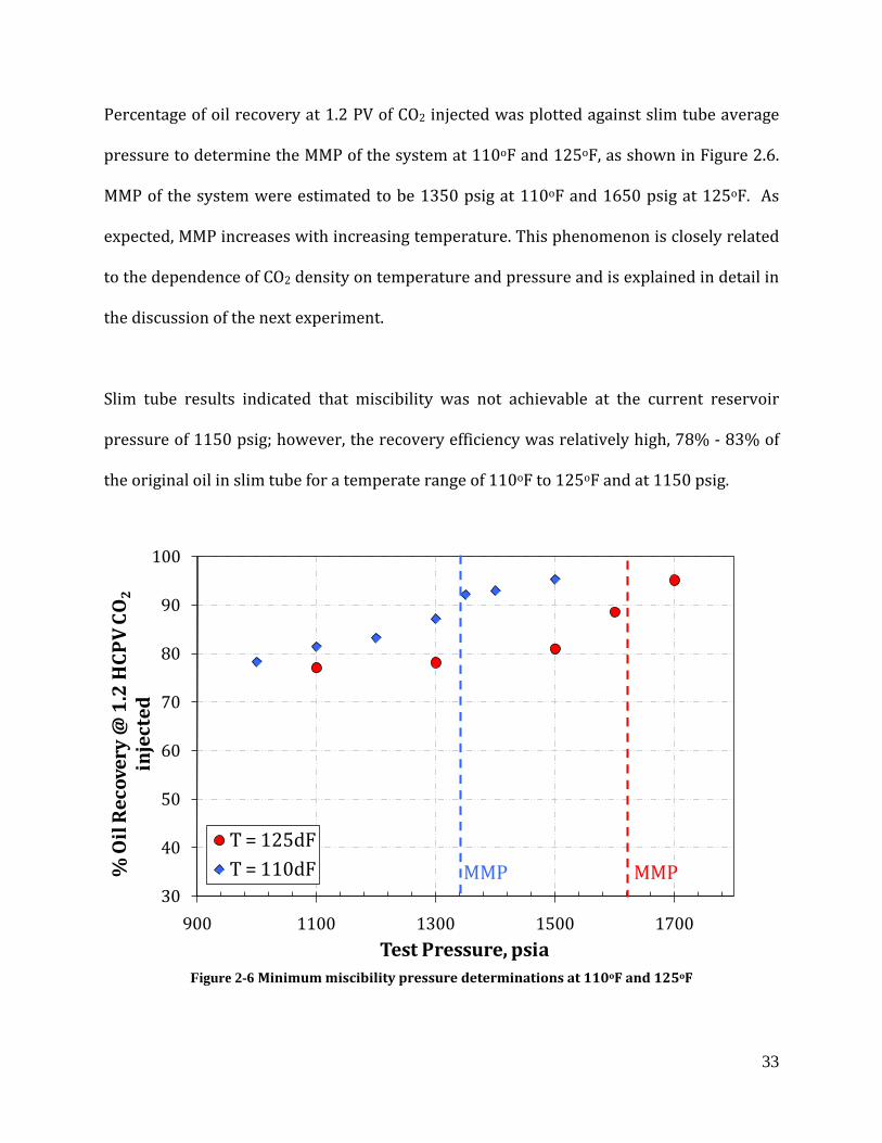
Percentage of oil recovery at 1.2 PV of CO2 injected was plotted against slim tube average

pressure to determine the MMP of the system at 110oF and 125oF, as shown in Figure 2.6.

MMP of the system were estimated to be 1350 psig at 110oF and 1650 psig at 125oF. As

expected, MMP increases with increasing temperature. This phenomenon is closely related

to the dependence of CO2 density on temperature and pressure and is explained in detail in

the discussion of the next experiment.

Slim tube results indicated that miscibility was not achievable at the current reservoir

pressure of 1150 psig; however, the recovery efficiency was relatively high, 78% - 83% of

the original oil in slim tube for a temperate range of 110oF to 125oF and at 1150 psig.

Figure 2-6 Minimum miscibility pressure determinations at 110oF and 125oF

30

40

50

60

70

80

90

100

900 1100 1300 1500 1700

% O

il R

ecov

ery

@ 1

.2 H

CP

V C

O2

inje

cted

Test Pressure, psia

T = 125dFT = 110dF MMP MMP

34

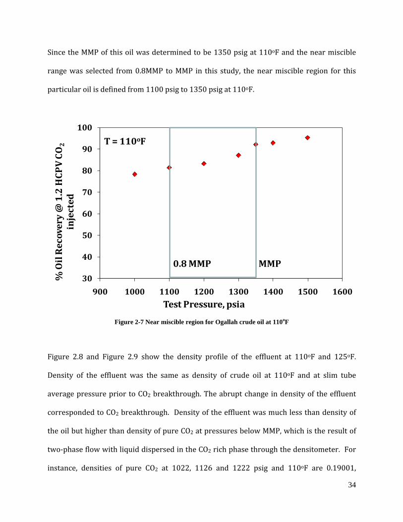
Since the MMP of this oil was determined to be 1350 psig at 110oF and the near miscible

range was selected from 0.8MMP to MMP in this study, the near miscible region for this

particular oil is defined from 1100 psig to 1350 psig at 110oF.

Figure 2-7 Near miscible region for Ogallah crude oil at 110oF

Figure 2.8 and Figure 2.9 show the density profile of the effluent at 110oF and 125oF.

Density of the effluent was the same as density of crude oil at 110oF and at slim tube

average pressure prior to CO2 breakthrough. The abrupt change in density of the effluent

corresponded to CO2 breakthrough. Density of the effluent was much less than density of

the oil but higher than density of pure CO2 at pressures below MMP, which is the result of

two-phase flow with liquid dispersed in the CO2 rich phase through the densitometer. For

instance, densities of pure CO2 at 1022, 1126 and 1222 psig and 110oF are 0.19001,

30

40

50

60

70

80

90

100

900 1000 1100 1200 1300 1400 1500 1600

% O

il R

ecov

ery

@ 1

.2 H

CP

V C

O2

inje

cted

Test Pressure, psia

MMP0.8 MMP

T = 110oF

35

0.23306 and 0.29009 g/cc, compared with densities of the effluent at the corresponding

pressures and temperature, 0.296, 0.415, and 0.527 g/cc.

Figure 2-8 Density profile of the effluent at 110oF

0

0.1

0.2

0.3

0.4

0.5

0.6

0.7

0.8

0.9

0.0 0.2 0.4 0.6 0.8 1.0 1.2

Den

sity

[gm

/cc]

PV of CO2 injected

P = 1509 psigP = 1417 psigP = 1375 psigP = 1323 psigP = 1222 psigP = 1126 psigP = 1022 psig

36

Figure 2-9 Density profile of the effluent at 125oF

2.2.4 Conclusions

MMP was estimated to be 1350 psig at 110oF and 1650 psig at 125oF. Miscibility is

therefore not achievable at the current reservoir pressure of 1150 psig.

Near miscible range is defined from 1000 psig to 1350 psig at 110oF in this study.

78% - 83% of the original oil in place was recovered at the current reservoir

pressure of 1150 psig and at a temperature range of 110oF to 125oF.

0.2

0.3

0.4

0.5

0.6

0.7

0.8

0.9

1.0

0 0.2 0.4 0.6 0.8 1 1.2

Den

sity

(g/c

c)

PV of CO2 injection

P = 1714 psigP = 1598 psigP = 1509 psigP = 1304 psigP = 1096 psig

37

2.3 Swelling/Extraction Tests

Swelling/extraction tests were performed to examine the oil recovery mechanisms in the

near-miscible region and to provide data to tune the phase behavior model. Swelling tests

were conducted to determine the relationship between saturation pressure, swelling factor

and CO2 volume injected. Extraction tests were carried out to examine the extraction of

liquid hydrocarbon into a CO2-rich phase and the effect of pressure on the extraction.

2.3.1 Experimental Setup and specifications

Figure 2-10 Experimental setup include (1) Gas cylinder (2) Isco Syringe pump (3) Fisher Isotemp circulator (4) Fisher Isotemp Immersion circulator (5) water bath (6) high pressure view cell (7) mixing bar (8) laboratory jack (9) computer (10) cathetometer with telescope (11) vacuum pump [13]

38

The schematic of swelling/extraction setup is shown in Figure 2.10. An Isco, Inc. 100DM

syringe pumps is used for CO2 injection. Temperature of the pump is controlled by a Fisher,

Inc. Isotemp circulator, model 3016 and measured by an Ertco-Eutechnic 5 digit

thermister, model 4400 in the range of 0-100oC.

The gas lines are heated using fiberglass covered heating tape, controlled by two variable

AC transformers, Staco Energy model 3PN1010B. Temperature of the gas lines is measured

using T-type thermocouples. Fiberglass cloth tape is used to prevent heat dissipation to the

surroundings.

The key component of this setup is the high pressure view cell with high pressure gauge

glass window allowing visual observations of fluids under experimental conditions. The

view cell is made of stainless steel and has a volume of 26 cc. The gauge glass window

allows a maximum temperature of 280oC and pressure of 4000 psi. Pressure in the view

cell is measured by a 5000 psi Heise DXD Series 3711 precision digital pressure transducer.

A 3.2mm diameter × 12.7 mm PTFE coated stir bar is placed inside the view cell. Mixing is

achieved by an external rare-earth magnet in a slot behind the cell raised and lowered by a

pulley system.

The view cell is immersed into the water bath by raising/lowering the platform jack. The

temperature of the water bath is adjusted by an immersion circulator Haake DC30/DL3

and a Fisher, Inc. Isotemp circulator, model 3016.

39

An Eberbach 5160 cathetometer is used to measure the height of the liquid in the view cell.

Figure 2-11 An actual image of the swelling/extraction experimental setup

2.3.2 Experimental Procedures

The pump was filled with CO2. Temperature of the pump was set constant and above the

critical temperature of CO2 (31.1oC). Pressure of the pump was set constant at the

maximum anticipated pressure. The pump automatically adjusted the volume of CO2 to

achieve constant temperature and pressure. Temperature of the gas lines was set at

40

temperature above the critical temperature of CO2 to avoid CO2 condensation inside the

lines. Temperature of the water bath was set constant at the desired temperature.

A predetermined volume of crude oil was carefully injected into the view cell to avoid

liquid droplets on the wall of the view cell. The view cell was attached to the gas lines and

then immersed into the water bath.

When the whole system was thermally equilibrated, the gas lines and the view cell were

quickly flushed with CO2 at low pressure to remove any residual gas or air.

A log file was created to record the following parameters: the pump condition

(temperature, pressure and volume of CO2), the temperature of the gas lines, the view cell

condition (temperature and pressure). The height of the liquid sample in the view cell was

recorded manually. Initially conditions should also be recorded manually.

The cell pressure was increased in discrete steps by CO2 injection from the top of the view

cell. CO2 injection was stopped when a desired pressure was achieved. CO2 flow rate was

kept slowly so that there was no PVT disturbance. This was done by checking the pump

pressure frequently to make sure the pump pressure did not drop too much from the set

pressure. Final volume of CO2 in the pump was recorded when CO2 flow rate is read zero.

During pressurization process, the time required for the contents in the view cell to

equilibrate under a particular pressure and temperature is minimized by magnetically

stirring. At that time, the following parameters were recorded manually: the height of the

41

liquid sample in the view cell, the pump condition (temperature, pressure & final volume of

CO2), temperature of gas lines and the view cell condition (temperature & pressure).

In the end, the view cell was cleaned with methylene chloride, acetone solution and blown

dry with compressed air.

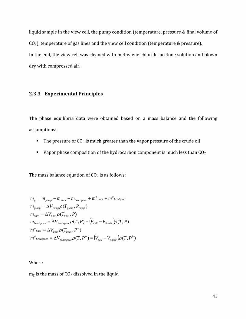
2.3.3 Experimental Principles

The phase equilibria data were obtained based on a mass balance and the following

assumptions:

The pressure of CO2 is much greater than the vapor pressure of the crude oil

Vapor phase composition of the hydrocarbon component is much less than CO2

The mass balance equation of CO2 is as follows:

Where

mg is the mass of CO2 dissolved in the liquid

( )

( ) ),(),(

),(

),(),(),(

),(

0PTVVPTVmPTVm

PTVVPTVmPTVm

PTVmmmmmmm

liquidcello

headspaceheadspaceo

olineslineslines

o

liquidcellheadspaceheadspace

lineslineslines

pumppumppumppump

headspaceo

lineso

headspacelinespumpg

ρρ

ρ

ρρρ

ρ

−=∆=

∆=

−=∆=∆=

∆=

++−−=

42

mpump is equal to the product of volume of CO2 displaced from the pump and density of CO2

at the pump constant temperature & pressure

mlines is equal to the product of volume of the lines and density of CO2 at temperature of the

lines & system equilibrium pressure

molines is equal to the product of volume of the lines and density of CO2 at temperature of the

lines & system initial pressure

mheadspace is equal to the product of volume of the headspace and density of CO2 at

temperature & pressure of the equilibrium system. The volume of the headspace is the

difference between volume of the cell and volume of the liquid in the cell.

moheadspace is equal to the product of volume of the headspace and density of CO2 at

temperature & pressure of the initial system. The volume of the headspace initially is the

difference between volume of the cell and initial volume of the liquid in the cell.

CO2 density was calculated using REFROP database which used the ultra-accurate Span-

Wagner equation of state.

Mole fraction of CO2 in the liquid phase was calculated as follows:

llgg

gg

lg

gg MmMm

Mmnn

nx

///+

=+

=

43

2.3.4 Apparatus Validation

The apparatus was verified by comparing experimental data obtained from this apparatus

with literature data for n-decane/CO2 mixture at 71.1oC by Ren et al. [13]. The

experimental data had excellent agreement with the literature data obtained from different

experimental methods.

Phase equilibrium data of CO2/n-decane at 71.1oC was obtained and shown in Table 2.3.

Run 1 Run 2 Pressure, psi xCO2 Pressure, psi xCO2 192.18 0.09609 209.43 0.10900 425.25 0.21070 434.97 0.22498 701.98 0.34940 643.68 0.32669 1005.55 0.50260 866.89 0.44391 1270.24 0.61657 1080.39 0.52821 1448.35 0.69121 1321.58 0.64927 1531.45 0.72330 1495.77 0.71555 1666.05 0.77723 1612.38 0.76148 1709.41 0.80048 1771.35 0.82829

Table 2.3 Phase equilibrium data of CO2/n-decane at 71.1oC

Analysis of this data was based on the assumption that the amount of liquid component in

the vapor phase is negligible. Although the composition of the vapor phase was not actually

analyzed in our experiments, it had been demonstrated earlier by Ren et al. [13] that the

percentage of n-decane in CO2 vapor phase was less than 0.13%. Figure 2.12 shows that

the p-x phase equilibrium of CO2/n-decane generated using this apparatus were

reproducible and in excellent agreement with literature data, Nagarajan & Robinson, Jr.

[14] and Jennings & Schucker [15], and therefore, it could be used for crude oil/CO2 system.

44

Figure 2-12 Comparison of liquid phase compositions for CO2+ n-decane system at 71.10oC (160oF) with literature data () this work () this work (∆) Nagarajan & Robinson Jr. (◊) Jennings & Schucker

2.3.5 Results and Discussions

Effect of each variable, temperature, pressure and initial volume on CO2/oil phase behavior

was investigated while holding others constant.

2.3.5.1 Effect of System Pressure

0

400

800

1200

1600

2000

0.0 0.2 0.4 0.6 0.8 1.0

Pre

ssu

re (

psi

)

Mole fraction of CO2 in the liquid phase

This work #1This work # 2Nagarajan & Robinson Jr.Jennings & Schucker

45

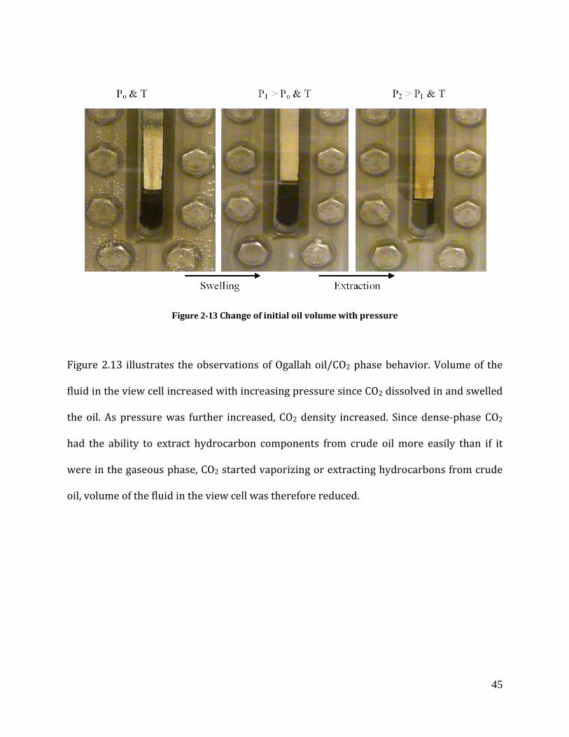
Figure 2-13 Change of initial oil volume with pressure

Figure 2.13 illustrates the observations of Ogallah oil/CO2 phase behavior. Volume of the

fluid in the view cell increased with increasing pressure since CO2 dissolved in and swelled

the oil. As pressure was further increased, CO2 density increased. Since dense-phase CO2

had the ability to extract hydrocarbon components from crude oil more easily than if it

were in the gaseous phase, CO2 started vaporizing or extracting hydrocarbons from crude

oil, volume of the fluid in the view cell was therefore reduced.

46

Figure 2-14 Effect of pressure on CO2 solubility and swelling factor at 110oF

Figure 2.14 shows the swelling/extraction curve for Ogallah/CO2 system at 110oF with the

sample size of 3 cc. The sample volume was about 11 % volume of the view cell. The

swelling factor (SF) of oil is the ratio of liquid volume at test pressure divided by the liquid

volume at atmospheric pressure and at 110oF. This value is determined by measuring the

change of the interface level as a result of CO2 dissolution in the oil or as a result of

hydrocarbon extracted into the CO2 rich vapor phase. Swelling factor was equal to 1 at

initial conditions. As a result of CO2 dissolution into the liquid phase, the liquid phase

swelled and the swelling factor was greater than 1. Maximum swelling occurred at 1158

psi, when volume of the liquid phase became 1.21 of its original volume with 0.728 mole

0.0

0.1

0.2

0.3

0.4

0.5

0.6

0.7

0.8

0.0

0.2

0.4

0.6

0.8

1.0

1.2

1.4

0 500 1000 1500 2000 2500

CO

2so

lub

ilit

y

Swel

lin

g Fa

ctor

Pressure, psi

Swelling FactorCO2 solubility

47

fraction of CO2 dissolved in the liquid phase. Major extraction started at approximately

1158 psi. As pressure increased, hydrocarbon components of the crude oil were removed

from the liquid phase, the liquid phase shrank and swelling factor was reduced. At 2035.2

psi, the volume of CO2 rich liquid phase shrank as much as 39.2 % of its original volume.

CO2 solubility is also plotted in Figure 2.15 as a function of pressure up to 1158 psi.

Calculations of CO2 solubility at pressures above 1158 psi are invalid since the assumption

that the components of the liquid phase do not vaporize does not hold true.

Extraction or vaporization of hydrocarbon components from crude oil appears to be the

primary oil recovery mechanism in the near miscible range, 1100 psig to 1350 psig.

2.3.5.2 Effect of System Temperature

Swelling/extraction experiments were performed under various temperatures from 105oF

to 125oF.

48

Figure 2-15 Effect of temperature on CO2 solubility

Figure 2-16 Effect of temperature on Swelling/ Extraction curves

0

200

400

600

800

1000

1200

1400

0.0 0.2 0.4 0.6 0.8 1.0

Pre

ssu

re, p

sia

Mole fraction of CO2 in the liquid phase

105F110F115F120F125F

0.0

0.2

0.4

0.6

0.8

1.0

1.2

1.4

0 500 1000 1500 2000 2500

Swel

lin

g Fa

ctor

Pressure, psi

105F110F115F120F125F

49

Effects of temperature on CO2 solubility and oil swelling/extraction curve are shown in

Figure 2.15 and Figure 2.16. CO2 solubility increased with increasing pressure and

decreased with increasing temperature. The rate of oil swelling decreased with increasing

temperature. The pressure at which oil swelling reached maximum or at which CO2 began

extracting components from crude oil increased with increasing temperature, ranging from

1158.8 psi to 1259.6 psi at a temperature range of 105oF to 125oF. The rate of oil shrinkage

decreased with increasing temperature.

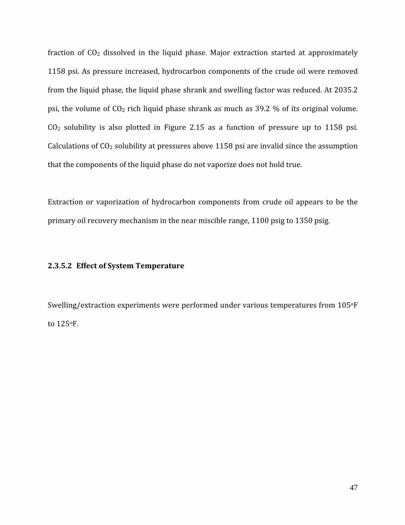
The temperature dependence of CO2/Ogallah crude oil phase behavior is explained by the

dependence of CO2 density on pressure and temperature. Density of CO2 as a function of

pressures and temperature are calculated using REFPROP and presented in Figure 2.18. It

takes higher pressure to achieve the equivalent CO2 density at a higher temperature; and

therefore, the pressure at which extraction starts increases with increasing temperature.

The rate of change of CO2 density with pressure is faster at lower temperature which

explains why the extraction rate is faster at lower temperature. Mass transfer between CO2

and oil phase is necessary to achieve dynamic miscibility. Since mass transfer between CO2

and oil phase starts earlier and faster at a lower temperature, MMP decreases with

decreasing temperature.

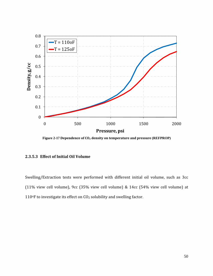
50

Figure 2-17 Dependence of CO2 density on temperature and pressure (REFPROP)

2.3.5.3 Effect of Initial Oil Volume

Swelling/Extraction tests were performed with different initial oil volume, such as 3cc

(11% view cell volume), 9cc (35% view cell volume) & 14cc (54% view cell volume) at

110oF to investigate its effect on CO2 solubility and swelling factor.

0

0.1

0.2

0.3

0.4

0.5

0.6

0.7

0.8

0 500 1000 1500 2000

Den

sity

, g/c

c

Pressure, psi

T = 110oFT = 125oF

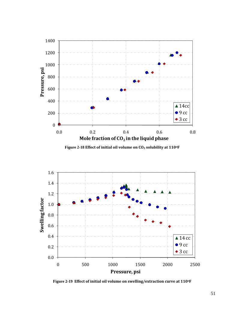
51

Figure 2-18 Effect of initial oil volume on CO2 solubility at 110oF

Figure 2-19 Effect of initial oil volume on swelling/extraction curve at 110oF

0

200

400

600

800

1000

1200

1400

0.0 0.2 0.4 0.6 0.8

Pre

ssu

re, p

si

Mole fraction of CO2 in the liquid phase

14cc9 cc3 cc

0.0

0.2

0.4

0.6

0.8

1.0

1.2

1.4

1.6

0 500 1000 1500 2000 2500

Swel

lin

g fa

ctor

Pressure, psi

14 cc 9 cc3 cc

52

The effect of initial oil volume on CO2 solubility and swelling factor at 110oF are shown in

Figure 2.18 and Figure 2.19. When the initial volume of crude oil in the view cell was large,

the amount of hydrocarbons extracted from the oil phase is considerably lower than when

the initial volume of crude oil in the view cell is small. The pressure at which significant

extraction began decreased with decreasing initial cell oil volume.

Similar observations have been reported by Hand et al. [16] and were first noted by Holm

and Josendal [4] in their work where a 30% of initial volume of sample was used for the

swelling test. Hand et al. [16] explained the effect of initial oil volume on

swelling/extraction curve by plotting the change in cell global gas composition with

pressure on a p-x diagram for the Flounder oil/CO2 system at 233oF.

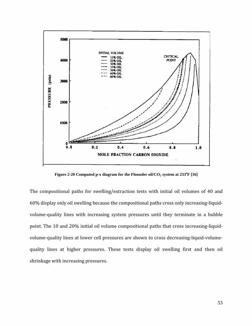
53

Figure 2-20 Computed p-x diagram for the Flounder oil/CO2 system at 233oF [16]

The compositional paths for swelling/extraction tests with initial oil volumes of 40 and

60% display only oil swelling because the compositional paths cross only increasing-liquid-

volume-quality lines with increasing system pressures until they terminate in a bubble

point. The 10 and 20% initial oil volume compositional paths that cross increasing-liquid-

volume-quality lines at lower cell pressures are shown to cross decreasing-liquid-volume-

quality lines at higher pressures. These tests display oil swelling first and then oil

shrinkage with increasing pressures.

54

Figure 2-21 Computed p-x diagram for Ogallah oil/ CO2 system at 110oF

Figure 2.21 shows a predicted p-x diagram for Ogallah oil/CO2 system at 110oF by

Winprop, CMG software. Also plotted are the experimental results, pressure vs. mole

fraction of CO2 for systems of 11%, 35% and 54% oil / CO2 at 110oF. Mole fraction of CO2

was determined by total mole of CO2 injected into the system divided by sum of total mole

of CO2 injected into the system and the moles of crude oil. The difference of

swelling/extraction curves between sample sizes is explained likewise, because the

compositional paths cross the liquid-volume-quality lines differently with increasing

pressure.

0

200

400

600

800

1000

1200

1400

0.0 0.1 0.2 0.3 0.4 0.5 0.6 0.7 0.8 0.9 1.0

Pre

ssu

re (

psi

a)

Mole fraction Carbon Dioxide

2-Phase boundary 80% Oil 40% Oil30% Oil 20% Oil 10% Oil3 cc (11% Oil) 9 cc (35% Oil) 14 cc (54% Oil)

55

2.3.6 Conclusions

CO2 solubility increases with increasing pressure and decreases with increasing

temperature. As a result of CO2 dissolution into the liquid phase, the liquid phase

swells. The degree of swelling depends on pressure and temperature.

The pressure at which CO2 begins to extract significant amounts of hydrocarbons

from crude oil increases with increasing temperature and with increasing initial oil

volume in the view cell. The amount of extraction increases with increasing vapor-

phase volume (decreasing initial oil volume) and decreases with increasing

temperature.

Significant extraction started at pressure of 1150 psig & 110oF. Extraction or

vaporization of hydrocarbons into the CO2 rich phase is the primary mechanism for

oil recovery in the near-miscible region, from 1100 psig to 1350 psig & at 110oF

Swelling/extraction tests provide valuable phase behavior data which is used later

to tune the phase behavior model.

2.4 Viscosity Measurements

A Cambridge Applied Systems’ high pressure viscometer (ViscoPro 2000 System 4-SPL-440

with Viscolab software) utilizes an electromagnetic concept to measure viscosity of pure

crude oil and/or crude oil/CO2 mixture. The accuracy of this viscometer was validated

earlier by Ahosseini et al. [17], first by using standard calibration solutions, then by

56

comparing viscosity values of n-hexane measured using this viscometer with literature

values.

2.4.1 Principle of Operation

The viscometer utilizes the principles of annular flow around an axially oscillating piston.

It contains two magnetic coils inside a stainless steel body. A low mass stainless steel

piston inside the measurement chamber is magnetically forced back and forth in the fluid.

As the piston is pulled toward the bottom of the measurement chamber, it forces the fluid

at the bottom of the chamber to flow around the piston toward the sensor opening where it

interchanges with the normal flow of the fluid. On the upward piston stroke, fresh process

fluid is pulled around the piston to the bottom of the measurement chamber. The time

required for the piston to move a fixed distance is related to the viscosity of the fluid in the

chamber. Temperature is measured continuously with the use of a platinum Resistance

Temperature Detector (RTD) mounted at the base of the measurement chamber.

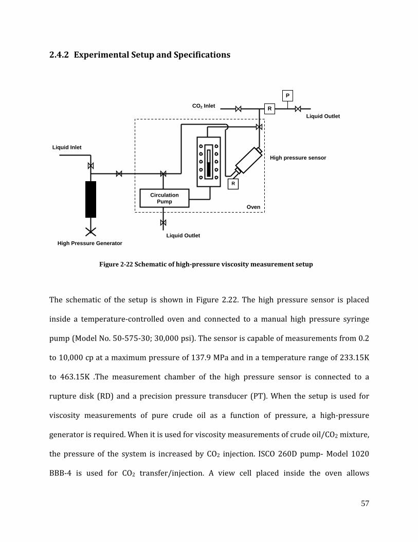
57

2.4.2 Experimental Setup and Specifications

The schematic of the setup is shown in Figure 2.22. The high pressure sensor is placed

inside a temperature-controlled oven and connected to a manual high pressure syringe

pump (Model No. 50-575-30; 30,000 psi). The sensor is capable of measurements from 0.2

to 10,000 cp at a maximum pressure of 137.9 MPa and in a temperature range of 233.15K

to 463.15K .The measurement chamber of the high pressure sensor is connected to a

rupture disk (RD) and a precision pressure transducer (PT). When the setup is used for

viscosity measurements of pure crude oil as a function of pressure, a high-pressure

generator is required. When it is used for viscosity measurements of crude oil/CO2 mixture,

the pressure of the system is increased by CO2 injection. ISCO 260D pump- Model 1020

BBB-4 is used for CO2 transfer/injection. A view cell placed inside the oven allows

Liquid Inlet

High Pressure Generator

Circulation Pump

R

P

RT

CO2 Inlet

Liquid Outlet

Liquid Outlet

High pressure sensor

Oven

Figure 2-22 Schematic of high-pressure viscosity measurement setup

58

observations of crude oil/CO2 interaction. During pressurization process, the time required

for the contents in the system to equilibrate under a particular pressure and temperature is

minimized by a circulation pump-Micropump, Inc. Model 415A.

Figure 2-23 An actual image of the high-pressure viscosity measurement setup

59

2.4.3 Experimental Procedures

Experimental procedures to measure oil viscosity and oil/CO2 mixture are outlined in the

following sections.

2.4.3.1 Oil Viscosity Measurement Procedure

Figure 2-24 A high pressure generator

The schematic in Figure 2.24 illustrates a very basic layout for using a high pressure

generator. A reservoir (R) is shown connected by means of valves and fittings to a

component (C) that is to be pressurized. With valve “B” closed and valve “A” open, the

handle of the high pressure generator is rotated counter-clockwise to create enough space

inside the cylinder body to store the crude oil. Valve “A” is then closed and valve “B” is

opened. By rotating the high pressure generator handle clockwise slowly, the piston will

compress the fluid to develop pressure in the component that is to be pressurized. If

sufficient pressure is not reached in one stroke, the system can be “recycled.” Valve “B” can

60

be closed in order to maintain pressure in the components. Valve “A” is then opened, and

fluid is again drawn into the Pressure Generator from the reservoir. Closing Valve “A” and

opening Valve “B” will now allow the Pressure Generator to be operated to develop

increased pressure in the component.

In this experimental setup, the oil was pumped into the cylinder body using the manual

high pressure syringe pump until the cylinder body is full. Excessive fluid introduction

would cause pressure buildup in the cylinder body; therefore, the system outlet must have

been opened before Valve “B” was opened to avoid damaging the sensor. The oil was

introduced into the system and into the measurement chamber, opening both Valve “A” and

Valve “B” and bypassing the high pressure generator. Temperature of the oven was set at

the desired temperature. When the system was at thermal equilibrium, the system was

purged to dislodge any potential bubbles. Temperature reading was taken from the RTD of

the viscometer. Valve “A” was closed, Valve “B” was opened when the system was

pressurized. The viscometer also needed to be turned off. By rotating the handle of the high

pressure generator slowly clockwise, pressure was developed in the system until a desired

pressure had reached. Viscosity reading was taken when temperature and pressure of the

system is stable.

61

2.4.3.2 Oil/CO2 Mixture Viscosity Measurement Procedure

Temperature of the oven is set constant at the desired temperature. Temperature of ISCO

pump was set constant at the desired temperature. Pressure of the pump was set constant

at the maximum anticipated pressure. Liquid was introduced into the measurement

chamber and into the view cell. When the system was at thermal equilibrium, the system

was purged to dislodge any potential bubbles. Temperature reading was taken from the

RTD of the viscometer. Viscometer needed to be turned off when CO2 was introduced into

the system. The system pressure was increased in discrete steps by CO2 injection from the

top of the view cell. CO2 injection was stopped when a desired pressure was achieved.

During pressurization process, a micropump was used to circulate the liquid inside the

system to help accelerating the mass transfer of the gas phase into the liquid phase.

Reading was taken when temperature and pressure of the system were stabilized.

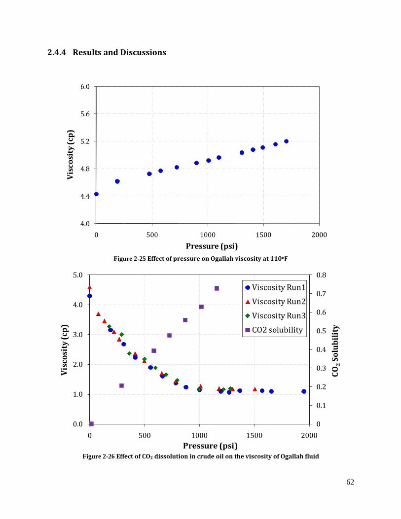
62

2.4.4 Results and Discussions

Figure 2-25 Effect of pressure on Ogallah viscosity at 110oF

Figure 2-26 Effect of CO2 dissolution in crude oil on the viscosity of Ogallah fluid

4.0

4.4

4.8

5.2

5.6

6.0

0 500 1000 1500 2000

Vis

cosi

ty (c

p)

Pressure (psi)

0

0.1

0.2

0.3

0.4

0.5

0.6

0.7

0.8

0.0

1.0

2.0

3.0

4.0

5.0

0 500 1000 1500 2000

CO2

Solu

bili

ty

Vis

cosi

ty (c

p)

Pressure (psi)

Viscosity Run1

Viscosity Run2

Viscosity Run3

CO2 solubility

63

Figure 2.25 shows the relationship of viscosity of pure crude oil with pressure at 110oF.

Figure 2.26 demonstrates the effect of CO2 dissolution into crude oil on viscosity of crude

oil at 110oF. As a result of CO2 dissolution into the liquid phase, viscosity of the liquid phase

was reduced. At pressures above 1000 psig, the effect of CO2 on oil viscosity is minimal. The

viscosity of the liquid phase was reduced as much as a factor of five in the near miscible

region, from 1100 psig to 1350 psig.

2.4.5 Conclusions

A nearly five-fold reduction in oil viscosity was achieved in the near-miscible region

with CO2 injection.

The reduction of oil viscosity improved the total mobility ratio between reservoir oil

and the displacing fluid, which will affect the recovery efficiency in a favorable way.

Viscosity measurements are useful in tuning the phase behavior model.

2.5 Phase Behavior Model

Equations of State (EOS) have been introduced widely to model and predict CO2-crude oil

phase behavior. An EOS is an algebraic relationship between pressure, temperature, and

molar volume for a single component or a mixture. Peng-Robinson EOS was used in this

study to describe the fluid properties and the oil/CO2 interaction.

64

22 2 bvbva

bvRTp

−+−

−=

The parameters a and b are defined using the following mixing rule for mixtures,

( )

∑

∑

∑

=

−=

=

iii

jjijjii

iii

bxb

adxaS

Sxa

1

Where, dij is an empirically determined interaction coefficient.

For pure components, the parameter ai and bi are expressed in terms of the critical

properties and the accentric factor:

( )( )

ccb

c

ccac

c

pRTbTT

pRTa

aa

//11

/

Ω=

−+=

Ω=

=

κα

α

Where, Ωa and Ωb are the EOS parameters with the default values of 0.45723553 and

0.077796074 for the PR EOS.

The κ is obtained from the following empirical correlations,

32 016666.0164423.048503.1379642.0 ωωωκ +−+=

While the application of the EOS to simple mixtures is relatively straightforward, crude oil

systems pose many seemingly insurmountable problems. The essential infinite number of

65

components contained in a typical crude oil makes it impossible to obtain a complete

chemical analysis. Standard oil analysis lumps all components heavier than C36 into a

single C36+ pseudo-component characterized by its average molecular weight and density.

Therefore, the parameters of the EOS were adjusted so that the EOS could reproduce the

laboratory-determined oil properties and the observed oil/CO2 interaction.

Slim tube model was constructed using 1-D compositional simulator with the tuned EOS.

Simulated slim tube results were compared with experimental slim tube results. The

following sections describe in detail how to develop the phase behavior model/slim tube

model in CMGTM software and how to characterize the phase behavior model to match with

experimental PVT data and slim tube results.

2.5.1 Phase Behavior Modeling using WINPROP

WinProp, a CMGTM software was utilized to build the phase behavior model. The EOS

requires the following properties for each component, critical pressure (Pc), critical

temperature (Tc), acentric factor (ω), and interaction coefficients between different

components (dij) to perform phase equilibrium calculations. The molecular weight (MW) is

also required to calculate mass densities. Additional factors such as the volume shifts τ, and

the equation-of-state parameters Ωa and Ωb can also be adjusted for each component to

enhance the equation of state predictions.

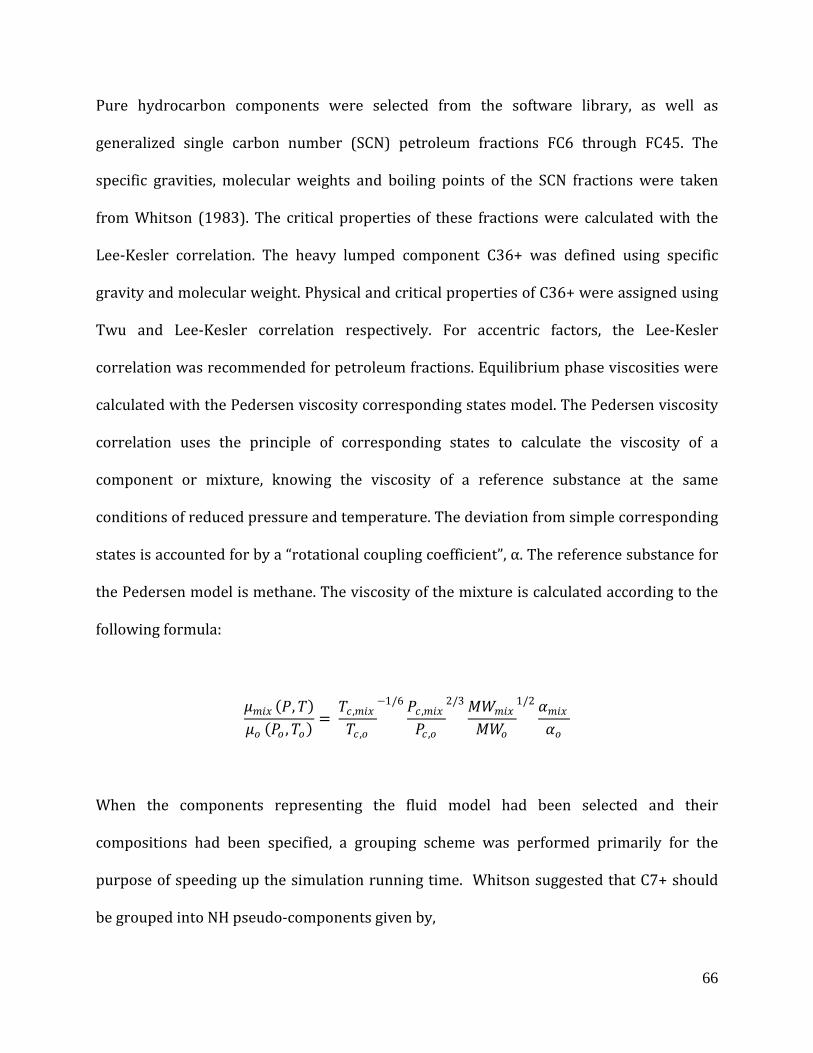
66

Pure hydrocarbon components were selected from the software library, as well as

generalized single carbon number (SCN) petroleum fractions FC6 through FC45. The

specific gravities, molecular weights and boiling points of the SCN fractions were taken

from Whitson (1983). The critical properties of these fractions were calculated with the

Lee-Kesler correlation. The heavy lumped component C36+ was defined using specific

gravity and molecular weight. Physical and critical properties of C36+ were assigned using

Twu and Lee-Kesler correlation respectively. For accentric factors, the Lee-Kesler

correlation was recommended for petroleum fractions. Equilibrium phase viscosities were

calculated with the Pedersen viscosity corresponding states model. The Pedersen viscosity

correlation uses the principle of corresponding states to calculate the viscosity of a

component or mixture, knowing the viscosity of a reference substance at the same

conditions of reduced pressure and temperature. The deviation from simple corresponding

states is accounted for by a “rotational coupling coefficient”, α. The reference substance for

the Pedersen model is methane. The viscosity of the mixture is calculated according to the

following formula:

𝜇𝜇𝑚𝑚𝑚𝑚𝑚𝑚 (𝑃𝑃,𝑇𝑇)𝜇𝜇𝑜𝑜 (𝑃𝑃𝑜𝑜 ,𝑇𝑇𝑜𝑜) =

𝑇𝑇𝑐𝑐 ,𝑚𝑚𝑚𝑚𝑚𝑚

𝑇𝑇𝑐𝑐 ,𝑜𝑜

−1/6 𝑃𝑃𝑐𝑐 ,𝑚𝑚𝑚𝑚𝑚𝑚

𝑃𝑃𝑐𝑐 ,𝑜𝑜

2/3 𝑀𝑀𝑀𝑀𝑚𝑚𝑚𝑚𝑚𝑚

𝑀𝑀𝑀𝑀𝑜𝑜

1/2 𝛼𝛼𝑚𝑚𝑚𝑚𝑚𝑚𝛼𝛼𝑜𝑜

When the components representing the fluid model had been selected and their

compositions had been specified, a grouping scheme was performed primarily for the

purpose of speeding up the simulation running time. Whitson suggested that C7+ should

be grouped into NH pseudo-components given by,

67

The groups are separated by molecular weights MI given by,

where N = CN of the heaviest fraction in the fluid description

I = 1 to NH

Therefore,

NH = 5 pseudo-groups

Group 1 < M1 = 138.303

M1 <Group 2 < M2 = 191.276

M2 < Group 3 < M3 = 264.539

M3 < Group 4 < M4 = 365.865

Finally a 8-component EOS fluid model was obtained after grouping:

C3 + iC4 + nC4 (1)

nC5+ iC5 (2)

C6 (3)

C7 – C9 (4)

C10 – C13 (5)

C14 – C18 (6)

C19 – C25 (7)

C26 – C36+ (8)

( )7log3.31 −+= NNH

( ) HNICNCI MMMM /

77/=

68

2.5.2 Equation of State Characterization

Figure 2.28 and Figure 2.29 present the experimental data and the simulated data after

tuning EOS parameters. Molecular weight (MW) of the heavy fraction was adjusted to

match the oil density. Coefficients of Pedersen viscosity correlation were adjusted to match

the oil viscosity. Binary interaction coefficients (BIC) between CO2 and the hydrocarbon

components as well as CO2 volume shift factor were adjusted to match saturation pressure

and swelling data. Table 2.5 shows the adjustment of each parameter to achieve the match.

Variable Lower Bound

Upper Bound

Initial Value

Final Value

MW C26 to C36+ 5.07E+02 7.60E+02 6.34E+02 5.98E+02 Volume shift of CO2 -1.54E-01 9.20E-01 0.00E+00 9.11E-01 BIC (C7-C9)-CO2 0.00E+00 2.00E-01 1.50E-01 0.00E+00 BIC (C10-C13)- CO2 0.00E+00 2.00E-01 1.50E-01 0.00E+00 Coefficient of viscosity correlation # 4 1.00E+00 2.22E+00 1.85E+00 1.04E+00 Coefficient of viscosity correlation # 5 4.14E-01 6.21E-01 5.17E-01 6.21E-01

Table 2.4 Adjustments of EOS parameters

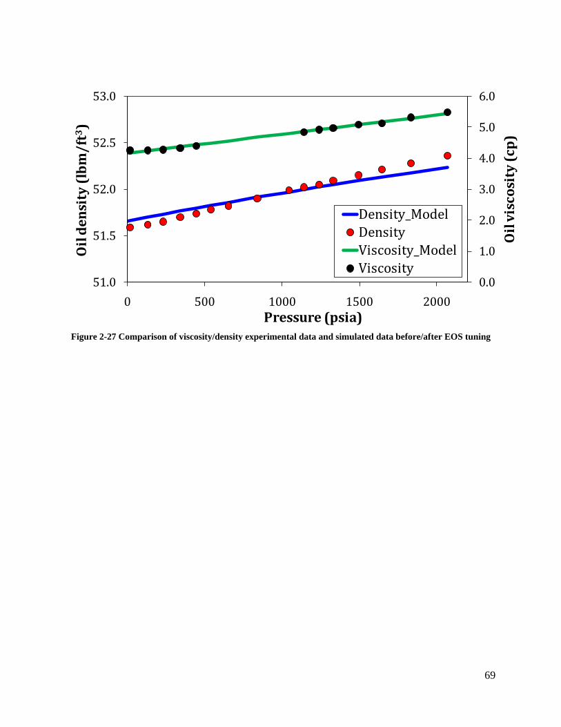
69

Figure 2-27 Comparison of viscosity/density experimental data and simulated data before/after EOS tuning

0.0

1.0

2.0

3.0

4.0

5.0

6.0

51.0

51.5

52.0

52.5

53.0

0 500 1000 1500 2000

Oil

vis

cosi

ty (

cp)

Oil

den

sity

(lb

m/f

t3)

Pressure (psia)

Density_ModelDensityViscosity_ModelViscosity

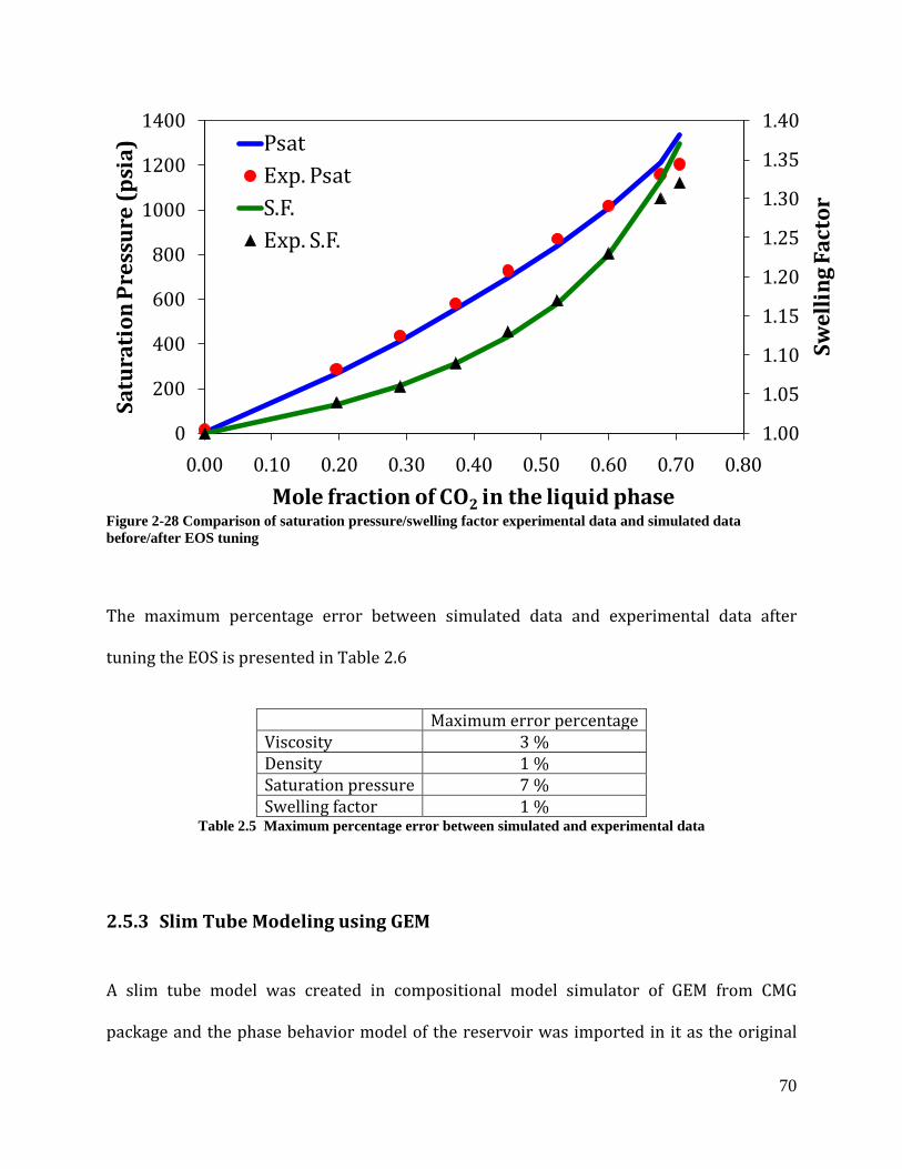
70

Figure 2-28 Comparison of saturation pressure/swelling factor experimental data and simulated data before/after EOS tuning

The maximum percentage error between simulated data and experimental data after

tuning the EOS is presented in Table 2.6

Maximum error percentage Viscosity 3 % Density 1 % Saturation pressure 7 % Swelling factor 1 %

Table 2.5 Maximum percentage error between simulated and experimental data

2.5.3 Slim Tube Modeling using GEM

A slim tube model was created in compositional model simulator of GEM from CMG

package and the phase behavior model of the reservoir was imported in it as the original

1.00

1.05

1.10

1.15

1.20

1.25

1.30

1.35

1.40

0

200

400

600

800

1000

1200

1400

0.00 0.10 0.20 0.30 0.40 0.50 0.60 0.70 0.80

Swel

lin

g Fa

ctor

Satu

rati

on P

ress

ure

(p

sia)

Mole fraction of CO2 in the liquid phase

PsatExp. PsatS.F.Exp. S.F.

71

saturated fluid of the tube. The slim tube was represented by a one dimensional linear

model using 320 grid blocks. The grid block sizes were 0.125 ft, 0.0185 ft and 0.0185 ft in I,

J, K direction respectively. One injector and one producer were incorporated at the ends of

the model.

Length, ft 40 Porosity, PV 0.367 Permeability, mD 4900 Pore Volume, cc 142.3 No. of blocks 320 Length of blocks, ft 0.125 Cross section, ft2 0.0003423 Each edge, ft 0.0185 Geometry Square Cross-section

Table 2.6 Slim tube model properties

The slim tube gas/oil relative permeability curves used in this model were obtained from

Negahban and Kremesec [18] and illustrated in Figure 2.27.

72

Figure 2-29 Relative permeability curve of oil-gas used in the simulation [18]

A number of slim tube displacements were simulated and compared with experimental

slim tube results in Figure 2.30.

0.0

0.2

0.4

0.6

0.8

1.0

0.0 0.2 0.4 0.6 0.8 1.0

kr-

Rel

ativ

e P

erm

eab

ilit

y

Sg

krg vs Sg

kro vs Sg

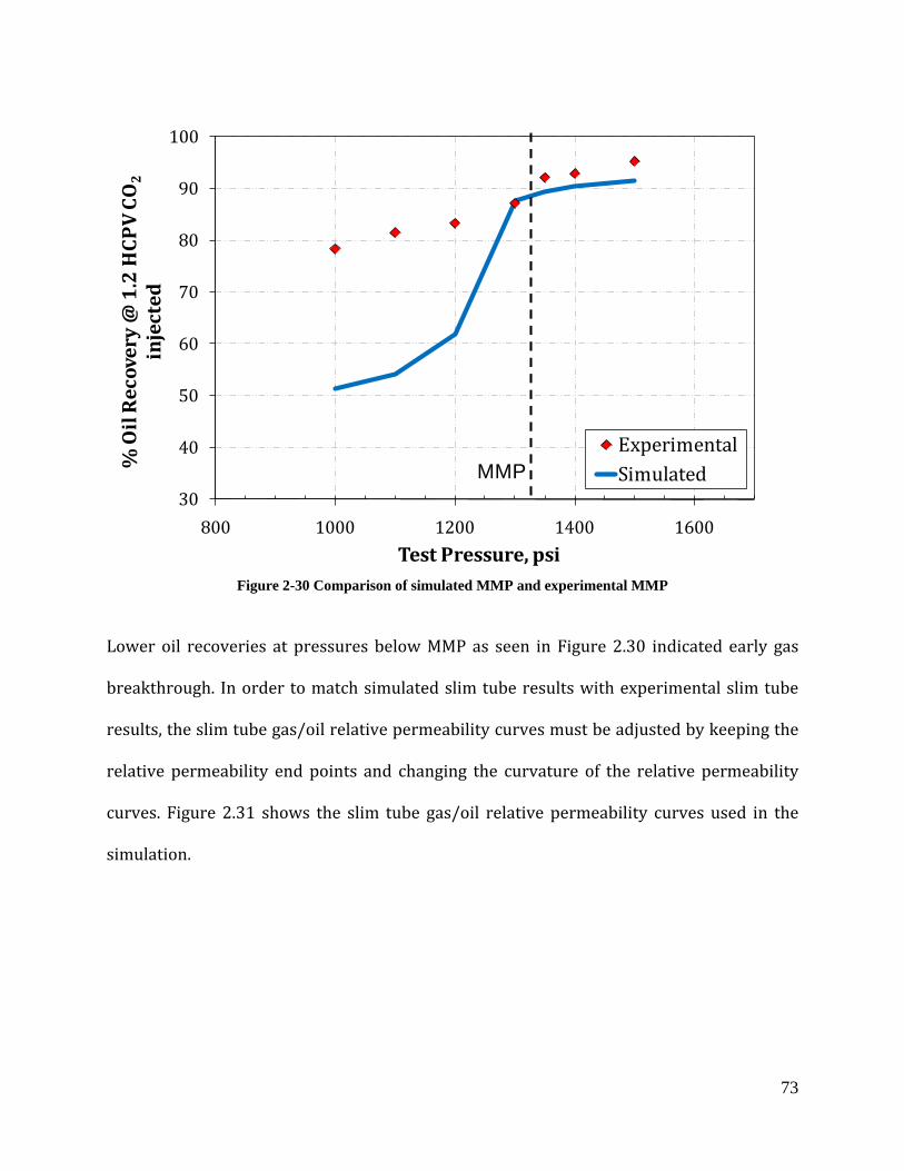
73

Figure 2-30 Comparison of simulated MMP and experimental MMP

Lower oil recoveries at pressures below MMP as seen in Figure 2.30 indicated early gas

breakthrough. In order to match simulated slim tube results with experimental slim tube

results, the slim tube gas/oil relative permeability curves must be adjusted by keeping the

relative permeability end points and changing the curvature of the relative permeability

curves. Figure 2.31 shows the slim tube gas/oil relative permeability curves used in the

simulation.

30

40

50

60

70

80

90

100

800 1000 1200 1400 1600

% O

il R

ecov

ery

@ 1

.2 H

CP

V C

O2

inje

cted

Test Pressure, psi

ExperimentalSimulatedMMP

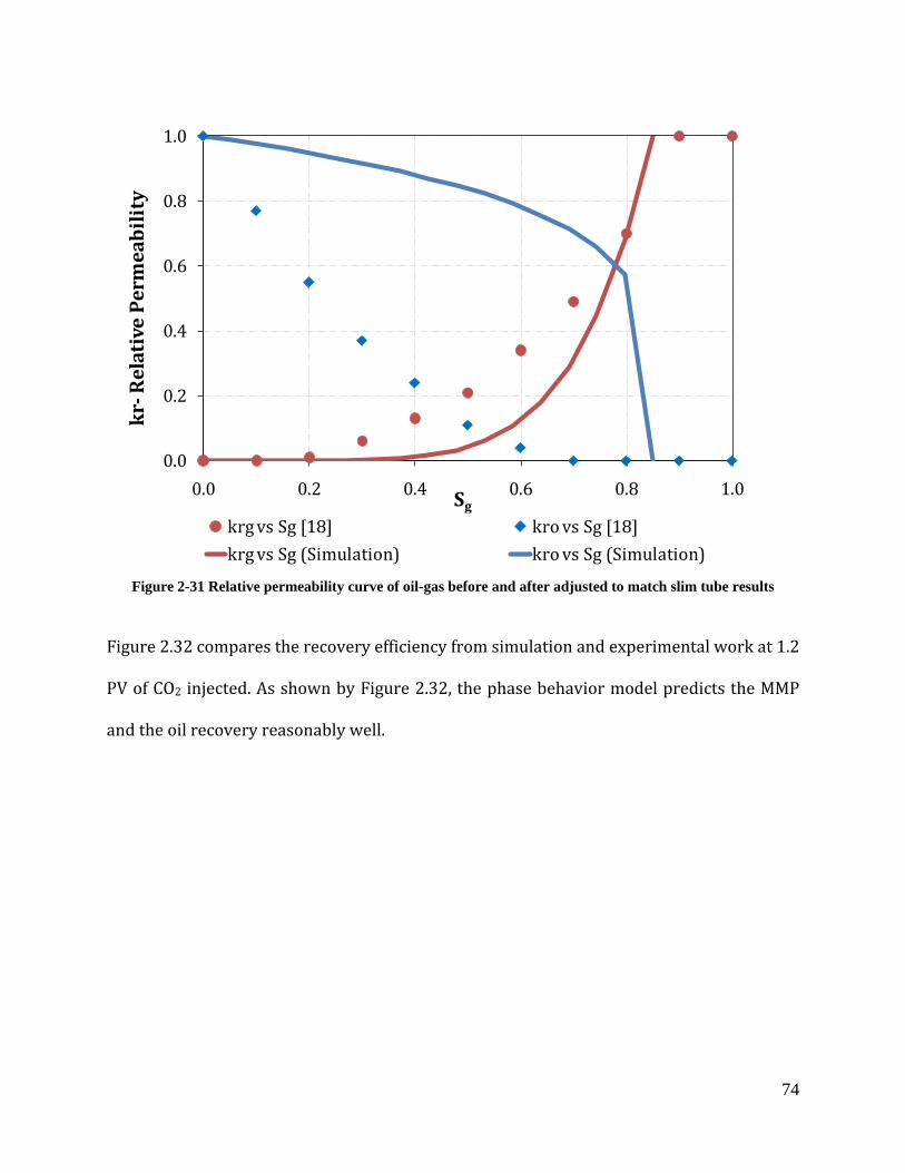
74

Figure 2-31 Relative permeability curve of oil-gas before and after adjusted to match slim tube results

Figure 2.32 compares the recovery efficiency from simulation and experimental work at 1.2

PV of CO2 injected. As shown by Figure 2.32, the phase behavior model predicts the MMP

and the oil recovery reasonably well.

0.0

0.2

0.4

0.6

0.8

1.0

0.0 0.2 0.4 0.6 0.8 1.0

kr-

Rel

ativ

e P

erm

eab

ilit

y

Sg

krg vs Sg [18] kro vs Sg [18]krg vs Sg (Simulation) kro vs Sg (Simulation)

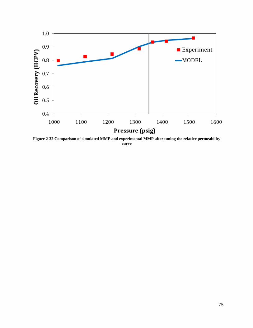
75

Figure 2-32 Comparison of simulated MMP and experimental MMP after tuning the relative permeability

curve

0.4

0.5

0.6

0.7

0.8

0.9

1.0

1000 1100 1200 1300 1400 1500 1600

Oil

Rec

over

y (H

CP

V)

Pressure (psig)

Experiment

MODEL

76

3 Core Flow Tests

Core flow tests were conducted under conditions that are more realistic than in slim tubes

and closer to the field conditions. They are virtually identical in procedure to the slim tube

displacement tests, except that a core sample replaced the bead-packed tube. The method

of conducting the tests and the results monitored are identical to the slim tube test.

CO2 core floods are difficult to interpret since linear displacements may or may not exhibit

characteristics common to a given reservoir such as dispersion, mobile water, wettability,

viscous fingering, gravity segregation, oil bypassing due to heterogeneity, and trapped oil

saturation. However, Orr et al. [19] suggested that core flow tests do seem appropriate for

answering at least three questions directly (1) Can CO2 mobilize tertiary oil under

conditions that are close to field displacement conditions than those occurring in slim tube

displacements? (2) What is the residual oil saturation in the swept zone of a CO2

displacement? (3) Does CO2 injection alter reservoir permeability by asphaltene

precipitation or dissolution of minerals?

3.1 Cores

Cores from Arbuckle reservoirs are limited. Berea sandstone, Baker dolomite and Arbuckle

dolomite rock samples were used in the core flow tests. Berea sandstone and Baker

dolomite were quarried rock samples whereas Arbuckle dolomite was cored sample from

77

Hadley well, Bemis-Shutts Field at Ellis County, Kansas. Before cores were epoxy encased

and cast inside an aluminum cylinder with high strength epoxy, at least three

measurements of the diameter and the length of each core were obtained. The average

value of the diameter and the length was used to calculate the area and the bulk volume of

each core. The dry weight of the core holder was recorded.

Upon completion of each core flow test, the cores were cleaned to restore to its initial

condition and reused for the next experiment. The core cleaning procedure is outlined as

follows:

The cores were successively cleaned with methylene chloride and methanol. At least

10 PV of methylene chloride followed by 10 PV of methanol was injected. The

sequence was repeated at least three times until the effluent was clear.

The cores were blown dry by CO2 and vacuumed to remove residual air/CO2.

The cores were fully saturated with either brine or crude oil, depending on which

type of core flow tests would be conducted. Brine was used for tertiary CO2 floods.

Crude oil was used for secondary CO2 floods.

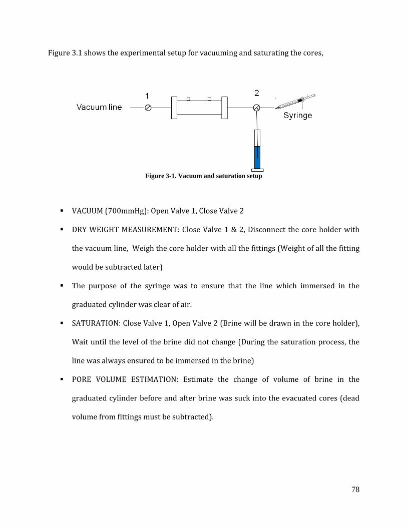
78

Figure 3.1 shows the experimental setup for vacuuming and saturating the cores,

Figure 3-1. Vacuum and saturation setup

VACUUM (700mmHg): Open Valve 1, Close Valve 2

DRY WEIGHT MEASUREMENT: Close Valve 1 & 2, Disconnect the core holder with

the vacuum line, Weigh the core holder with all the fittings (Weight of all the fitting

would be subtracted later)

The purpose of the syringe was to ensure that the line which immersed in the

graduated cylinder was clear of air.

SATURATION: Close Valve 1, Open Valve 2 (Brine will be drawn in the core holder),

Wait until the level of the brine did not change (During the saturation process, the

line was always ensured to be immersed in the brine)

PORE VOLUME ESTIMATION: Estimate the change of volume of brine in the

graduated cylinder before and after brine was suck into the evacuated cores (dead

volume from fittings must be subtracted).

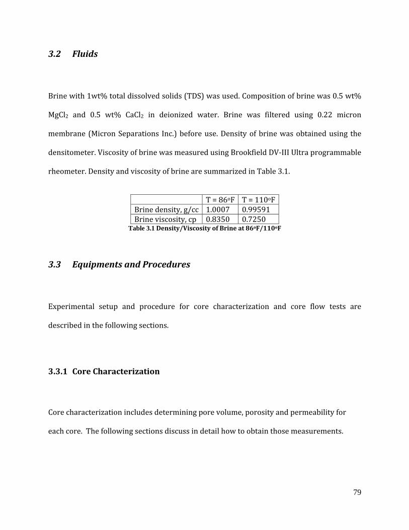
79

3.2 Fluids

Brine with 1wt% total dissolved solids (TDS) was used. Composition of brine was 0.5 wt%

MgCl2 and 0.5 wt% CaCl2 in deionized water. Brine was filtered using 0.22 micron

membrane (Micron Separations Inc.) before use. Density of brine was obtained using the

densitometer. Viscosity of brine was measured using Brookfield DV-III Ultra programmable

rheometer. Density and viscosity of brine are summarized in Table 3.1.

T = 86oF T = 110oF Brine density, g/cc 1.0007 0.99591 Brine viscosity, cp 0.8350 0.7250

Table 3.1 Density/Viscosity of Brine at 86oF/110oF

3.3 Equipments and Procedures

Experimental setup and procedure for core characterization and core flow tests are

described in the following sections.

3.3.1 Core Characterization

Core characterization includes determining pore volume, porosity and permeability for

each core. The following sections discuss in detail how to obtain those measurements.

80

3.3.1.1 Pore Volume Measurements

As mentioned earlier, pore volume can be approximated by the change of volume of brine

in the graduated cylinder before and after brine was drawn into the evacuated cores. Pore

volume of each core, however, can be determined more accurately by two ways,

gravimetric method and tracer tests. In the gravimetric method, the pore volume of each

core was computed based on the weight difference of the core before and after brine was

imbibed into the dry and evacuated core. In the tracer tests, concentration of tracer

solution is analyzed; equal area technique is utilized to calculate pore volume of each core.

Both techniques are discussed in detail in the following sections.

3.3.1.1.1 Gravimetric Method

The core holder was weighed before and after fully saturated with brine. Pore volume of

each core was calculated as follows:

ρds WWPV −

=

Where,

PV = pore volume (cc)

Ws = weight of the core holder when it is 100% saturated with brine (g)

Wd = weight of the core holder when it is dry (g)

81

ρ = density of brine at the testing temperature (g/cc)

Core porosities were calculated as follows:

BVPV

=φ

Where,

Φ= porosity

PV = pore volume (cc)

BV = bulk volume (cc)

3.3.1.1.2 Tracer Tests

Tracer tests were performed to confirm the pore volume of a core. A tracer is an injected

substance that is both measurable (e.g. through UV-visible detection) and conserved (i.e.

not retained, destroyed or created by the core). 1 wt% MgNO3 was used as a tracer in this

study. If tracer concentration is recorded at the core outlet and plotted as a function of

time, an S-shaped curve will form. The S-shaped curve is caused by dispersion of one fluid

into another; otherwise, there would be an instantaneous change in tracer concentration at

breakthrough. Tracer data is typically normalized to scale the tracer concentration values

from zero to one. A typical normalized tracer curve is shown in Figure 3.2.

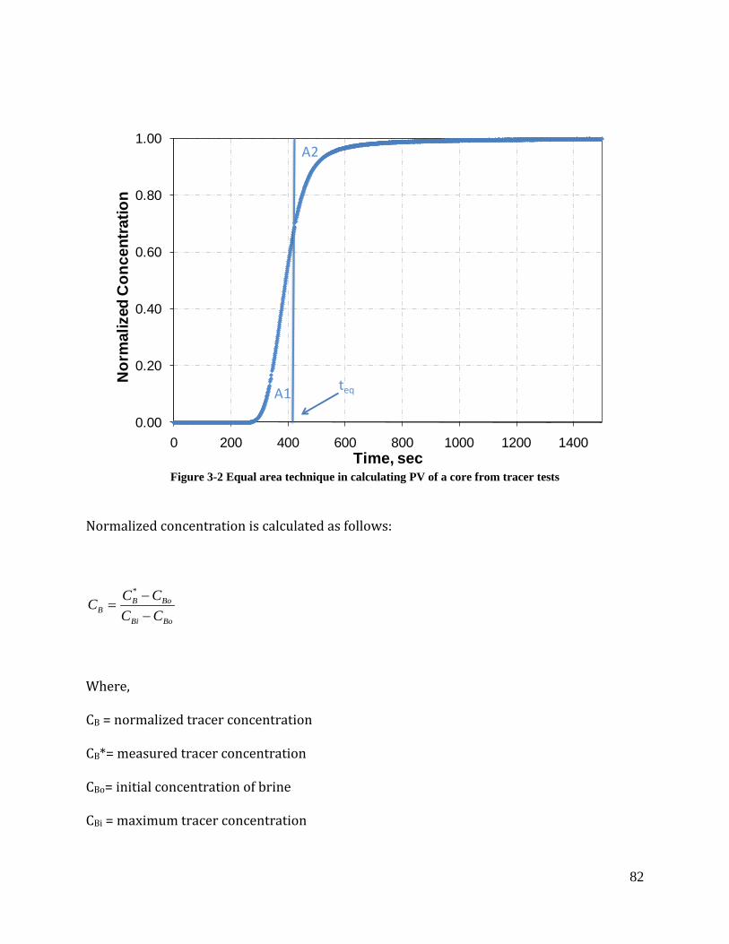
82

Figure 3-2 Equal area technique in calculating PV of a core from tracer tests

Normalized concentration is calculated as follows:

BoBi

BoBB CC

CCC−−

=*

Where,

CB = normalized tracer concentration

CB*= measured tracer concentration

CBo= initial concentration of brine

CBi = maximum tracer concentration

0.00

0.20

0.40

0.60

0.80

1.00

0 200 400 600 800 1000 1200 1400

Nor

mal

ized

Con

cent

ratio

n

Time, sec

teqA1

A2

83

Equal-area technique is utilized to compute PV of a core as follows:

( )( ) doeq VqttPV −×−=

Where,

Vd = any dead volume (cc)

q = tracer flowrate (cc/min)

to = time at which tracer injection starts (min)

teq= time at which equal area under each side of the curve reaches, A1 = A2

Areas on each side of the tracer concentration, A1 & A2, were calculated using trapezoidal

rule. teq is at A1 = A2.

Several primary assumptions are made in tracer testing [3]

• Fluid B is displacing Fluid A, and the two fluids are miscible

• There is no viscous fingering of one fluid into another, only dispersion

• Flow is single phase

• Fluids are incompressible

• Fluids are of equal density

• Flow is in only one direction

• Fluid velocity is constant

• Flow is through a porous medium of constant porosity and cross-sectional area

84

Figure 3-3 Schematic of tracer setup

Figure 3.3 shows the schematic of the tracer setup. The injection system consists of an

ISCO, Inc. 260DM syringe pump (for mineral oil transfer and injection) and two transfer

cylinders (for tracer solution/brine/mineral oil storage). 1 wt% MgNO3 was used as a

tracer. The inlet of the core holder is connected to the injection system. The three-way

valve allows switching the flow between tracer solution and brine. The outlet of the core is

connected to an UV-visible detector. The UV-visible detector should be turned on and set at

a wavelength of 302 nm at least an hour prior tracer tests. The flow cell of the detector

should be cleaned by methylene chloride, followed by acetone and finally brine injection.

85

Brine passed through core at a constant flow rate until UV-visible detector read a steady

concentration value. At this point, the detector was zeroed and the three-way valve was

switched to tracer injection. The switchover time needed to be recorded manually.

When tracer concentration did not change over time, the valve was switched back to non-

tracer injection to displace the tracer solution from the core. Again, the switchover time

needed to be recorded manually.

3.3.1.2 Permeability Measurements

Pressure drop was recorded during the brine flow tests and used to calculate permeability

of each core based on Darcy’s Law:

∆

=

PL

Aqk µ

Where,

q = flow rate of fluid through the core (cc/sec)

k = permeability (Darcy)

A= area (cc)

µ = viscosity of the fluid (cp)

∆P = pressure drop (atm)

L = length (cm)

86

Brine flow rates were varied to confirm the permeability of each core.

3.3.2 Core Floods

3.3.2.1 Experimental Setup

Figure 3-4 Schematic of core flood setup

The core flood setup is shown in Figure 3.4. The core flood displacement setup consists of a

core holder, injection system, a high-pressure densitometer, a production system and a

computerized data acquisition system. The temperature of the system is maintained in a

Linberg/Blue M oven with Eurotherm temperature control.

Gas

Oil

ISCO Pump

ISCO Pump

Quizix Pump

BPR

DPT

Test Oil

CO2

Brine

87

The injection system consists of a Parker transfer cylinder (oil storage), two Isco, Inc.

260DM syringe pumps (oil/CO2 transfer and injection) and a Quizix Pump (brine transfer

and injection). The capacity of the transfer cylinder is 485 cc. The cylinder can withstand a

maximum pressure of 3000 psi.

The production system consists of a back-pressure regulator, connected to the outlet of the

core holder, to set/control the system pressure. Back pressure regulator models BPR-50 is

a dome-load type, which controls the upstream back pressure to whatever pressure is

applied to the dome. It is designed to operate using compressed gas in the dome and water,

oil, gas in the body. A high pressure bottle of inert gas, such as nitrogen, is required to

pressurize the unit. The back pressure regulator has a working pressure of 5000 psi at

200oF (93oC).

During the experiment, the core effluent was flashed to atmospheric pressure at the outlet

of the back-pressure regulator. The separator fluid was collected in glassware designed for

different stages of displacement. The amount of fluids produced was determined

volumetrically and/or gravimetrically.

Three Valydine pressure transducers are installed to measure pressures at different

locations, such as pressure drop across the core, upstream pressures (CO2/oil/brine

pressure), and downstream pressure (back-pressure regulator pressure). The transducers

measure pressures up to 2500 psi with the accuracy of 0.25% of their full scale (0-2500

psi).

88

3.3.2.2 Experimental Procedures

Two sets of core flood experiments were performed, secondary CO2 flooding and tertiary

CO2 flooding to investigate the effect of operating pressure, in the near-miscible range on

the recovery efficiency and to investigate the effect of mobile water on the recovery

efficiency. In each set of experiment, core flood tests were carried out for a range of

pressures and at the reservoir temperature of 110oF. Crude oil/brine/CO2 injection

volumes were kept the same to compare the amount of oil recovered in each run.

3.3.2.3 Displacement Rate Selection

Residual oil saturation in laboratory core floods has been observed to depend on CO2 flow

rate. Poorer oil recoveries were found at increasing frontal advance rates by Shelton and

Schneider [20]. Low flow rate allows CO2 to diffuse through the network of pores and hence

increase oil recovery by swelling and/or vaporizing. Crude oil/brine/CO2 displacement

rates were selected 0.1cc/min to keep the capillary number as low as 10-6 and to achieve

realistic unit displacement efficiency in laboratory CO2 displacement.

89

3.4 Results and Discussions

3.4.1 Core Characterization Results

Table 3.2 presents the properties of Berea sandstone, Baker dolomite and Arbuckle

dolomite. Bulk volumes of the cores were calculated from at least three measurements of

diameters and lengths. Pore volume of each core was averaged from the results of tracer

tests and gravimetric methods, and from which porosity of each core was calculated.

Permeability to brine was calculated using different flow rates and averaged.

Type Berea sandstone

A1 Berea sandstone

A2 Arbuckle dolomite

Baker dolomite

Length (cm) 5.86 14.67 5.97 8.07 Cross section (cm)

2.53 3.86 2.46 2.34

Area (cm2) 5.01 11.67 4.75 4.30 Pore volume (cc) 5.80 34.72 6.05 7.20 Porosity 19.7 % 20.28% 21.3% 20.7% Permeability (mD)

238.5 369.04 2.5 89.7

Table 3.2 Core properties

3.4.2 Core Floods Results

3.4.2.1 Secondary CO2 Flooding

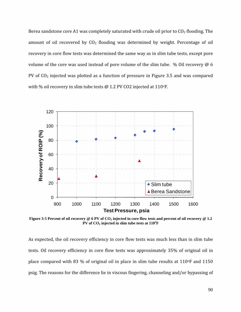
90

Berea sandstone core A1 was completely saturated with crude oil prior to CO2 flooding. The

amount of oil recovered by CO2 flooding was determined by weight. Percentage of oil

recovery in core flow tests was determined the same way as in slim tube tests, except pore

volume of the core was used instead of pore volume of the slim tube. % Oil recovery @ 6

PV of CO2 injected was plotted as a function of pressure in Figure 3.5 and was compared

with % oil recovery in slim tube tests @ 1.2 PV CO2 injected at 110oF.

Figure 3-5 Percent of oil recovery @ 6 PV of CO2 injected in core flow tests and percent of oil recovery @ 1.2

PV of CO2 injected in slim tube tests at 110oF

As expected, the oil recovery efficiency in core flow tests was much less than in slim tube

tests. Oil recovery efficiency in core flow tests was approximately 35% of original oil in

place compared with 83 % of original oil in place in slim tube results at 110oF and 1150

psig. The reasons for the difference lie in viscous fingering, channeling and/or bypassing of

0

20

40

60

80

100

120

900 1000 1100 1200 1300 1400 1500 1600

Rec

over

y of

RO

IP (%

)

Test Pressure, psia

Slim tube Berea Sandstone

91

oil due to core heterogeneities in a core displacement test. Another theory might be the

core was too short for the multiple contact miscibility to develop. Rathmell et al. [21]

reported that the average residual oil for the entire core was observed to decrease with

increasing core length and suggested that up to several feet were required to generate the

miscible transition zone before oil recovery representative of CO2 miscible displacement

was achieved. Therefore, further experiments with longer cores need to be performed to

verify this.

3.4.2.2 Tertiary CO2 flooding

Three groups of rock samples were used in this series of test. Berea sandstone, Arbuckle

dolomite and Baker dolomite were first saturated with brine, followed by crude oil

injection to residual water saturation and brine injection to residual oil saturation prior to

CO2 flooding. At least 10 PV of crude oil/brine injection was used to establish a steady

residual fluid saturation. The amount of oil recovered by CO2 flooding was determined

volumetrically. Table 3.3 to Table 3.6 summarizes CO2 tertiary core flood results for Berea

sandstone/ Arbuckle dolomite/ Baker dolomite at 110oF. Calculations of residual water

saturation (Swr), residual oil saturation due to water-flooding (Sorw), residual oil saturation

due to CO2 flooding (Sorm), and residual water saturation due to CO2 flooding (Swf) are based

on material balance. A sample is attached in the Appendix.

Pressure Swr Sorw Sorm Swf Recovery 1-(Sorm/Sorw) (psig)

92

905 0.32 0.48 0.31 0.37 35.71 1104 0.32 0.50 0.29 0.39 41.38 1198 0.32 0.48 0.26 0.41 46.43 1317 0.32 0.50 0.21 0.34 58.62 1413 0.32 0.48 0.21 0.34 57.14

Table 3.3 Tertiary CO2 flood results in Ogallah/Berea sandstone A1 at 110oF

Pressure Swr Sorw Sorm Swf Recovery 1-(Sorm/Sorw) (psig) 900 0.32 0.38 0.31 0.43 20.45 1099 (Run 1) 0.35 0.35 0.26 0.46 27.87 1100 (Run2) 0.36 0.36 0.26 0.41 28.13 1206 0.33 0.36 0.20 0.44 45.97 1314 0.36 0.33 0.13 0.51 60.18 Table 3.4 Tertiary CO2 flood results in Ogallah/Berea sandstone A2 at 110oF

Pressure Swr Sorw Sorm Swf Recovery 1-(Sorm/Sorw) (psig) 901 0.38 0.41 0.17 0.51 60.00 1100 0.38 0.41 0.17 0.55 60.00 1200 0.45 0.33 0.08 0.64 75.00 1305 0.45 0.33 0.07 0.64 80.00 1407 0.38 0.38 0.10 0.53 73.91

Table 3.5 Tertiary CO2 flood results in Ogallah/Arbuckle dolomite at 110oF

Pressure Swr Sorw Sorm Swf Recovery 1-(Sorm/Sorw) (psig) 905 0.28 0.39 0.15 0.44 60.71 1109 0.31 0.38 0.13 0.41 66.67 1201 0.34 0.35 0.10 0.45 72.00 1303 0.37 0.35 0.07 0.53 80.00 1402 0.37 0.32 0.07 0.47 78.26 Table 3.6 Tertiary CO2 flood results in Ogallah/ Baker dolomite at 110oF

Figure 3.6 compares percent of oil recovery @ 6 PV of CO2 injected as a function of pressure

for Berea sandstone A1, Baker dolomite and Arbuckle dolomite at 110oF. The recovery

efficiency was similar between two dolomite cores but substantially higher than that in

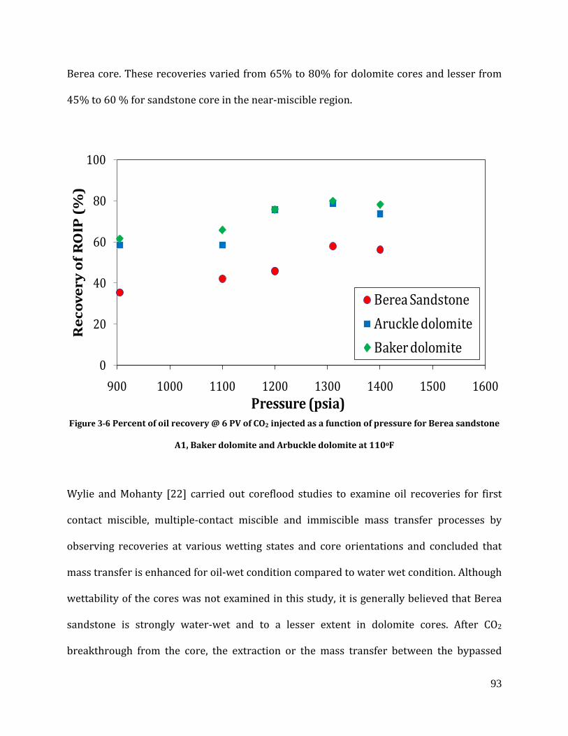
93

Berea core. These recoveries varied from 65% to 80% for dolomite cores and lesser from

45% to 60 % for sandstone core in the near-miscible region.

Figure 3-6 Percent of oil recovery @ 6 PV of CO2 injected as a function of pressure for Berea sandstone

A1, Baker dolomite and Arbuckle dolomite at 110oF

Wylie and Mohanty [22] carried out coreflood studies to examine oil recoveries for first

contact miscible, multiple-contact miscible and immiscible mass transfer processes by

observing recoveries at various wetting states and core orientations and concluded that

mass transfer is enhanced for oil-wet condition compared to water wet condition. Although

wettability of the cores was not examined in this study, it is generally believed that Berea

sandstone is strongly water-wet and to a lesser extent in dolomite cores. After CO2

breakthrough from the core, the extraction or the mass transfer between the bypassed

0

20

40

60

80

100

900 1000 1100 1200 1300 1400 1500 1600

Re

cove

ry o

f R

OIP

(%

)

Pressure (psia)

Berea SandstoneAruckle dolomiteBaker dolomite

94

region and flowing CO2 becomes more important to extract the remaining oil inside the

core. The findings from Wylie’s study may explain why the recovery efficiency is higher in

dolomite cores than in sandstone cores for this particular experiment.

As mentioned earlier, crude oil/brine/CO2 displacement rates were selected 0.1cc/min to

keep the capillary number as low as 10-6 and to achieve realistic unit displacement

efficiency in laboratory CO2 displacement. However, since the residual oil saturation in

Berea sandstone A1 was as high as 50%, different displacement rate was selected to drive

the residual oil saturation further down. Crude oil flow rate was selected 1cc/min for the

first 2 PV and 2cc/min for another 4PV during brine displacement test by crude oil. Brine

flow rate was selected 1cc/min for 6 PV during crude oil displacement test by brine. High

pressure drop drove the waterflood residual oil saturation from 0.48-0.50 for Berea

sandstone A1 to 0.33-0.38 for Berea sandstone A2. CO2 flow rate was selected 0.1cc/min

for 6 PV. At current reservoir pressure 1150 psig, the recovery efficiency of Berea

sandstone A1 was approximately 45% whereas the recovery efficiency of Berea sandstone

A2 was 35%. Core flow test was repeated at 1100psig & 110oF for Berea sandstone A2.

Core flow tests at 1100psig and 110oF were reproducible. It is not possible to compare the

recovery efficiency in Berea long core and Berea short core since the pore volume and the

residual oil saturation after waterflooding of two cores were different.

95

Figure 3-7 Recovery efficiency of Berea sandstones A1 & A2 at 1100 psig & 110oF.

3.4.2.3 Effect of Water Saturation on Oil Recovery Efficiency

The residual oil phase after waterflooding and before initiating tertiary CO2 injection exists

in the porous media as a trapped, disconnected phase surrounded by water. High mobile

water saturations affect the CO2 displacement efficiency in an unfavorable way because

water prevents CO2 from contacting and mobilizing the oil, however to what extent is still

unclear.

0

10

20

30

40

50

60

70

800 900 1000 1100 1200 1300 1400

% O

il R

ecov

ery,

1-(

Sorm

/Sor

w)

System Pressure, psi

Berea Short Core

Berea Long Core-Run 1

Berea Long Core - Run 2

96

Shelton and Schneider [20] studied the effect of mobile water saturations on oil recovery in

CO2 miscible displacement tests on sandstone cores and concluded that miscible

displacement performances for secondary and tertiary conditions are equivalent.

Tiffin and Yellig [23] evaluated continuous CO2 injection in secondary and tertiary

displacement modes using water-wet and oil wet cores and concluded that mobile water

from a previous waterflooding did not significantly change either the overall recovery or

the mechanism by which miscibility was developed from what was observed in secondary

CO2 displacement tests.

In another study by Campbell and Orr [24], however, visual observations of pore-level

displacement events indicate that CO2 displaced oil much more efficiently in both first

contact and multiple contact miscible displacements when water was absent. Water from a

prior water flood restricted access of CO2 to the oil. The low viscosity of CO2 aggravated

effects of high water saturations because CO2 did not displace water efficiently. Given

enough time, CO2 did however contact trapped oil by diffusing through water to reach, to

swell and to reconnect isolated droplets.

Also, studies by Stalkup [25] have indicated that higher water saturations increase both

the amount of bypassed oil and the longitudinal dispersion coefficient. He also presented

that the dominant mechanisms for recovery of the water blocked oil are miscible flushing

by solvent and recovery by molecular diffusion. Furthermore, Stalkup’s results indicate

97

that the effect of oil trapping by water will be more significant in laboratory core

experiments than in field scale operations.

Shyeh-Yung et al. [7] studied the effect of initial water saturation by comparing secondary

CO2 floods with tertiary CO2 floods. Initial water saturation was about 40% for secondary

CO2 floods and a water-flood preceding a tertiary CO2 floods usually raised the water

saturation to about 75%. Secondary CO2 floods showed more oil recovery than CO2 tertiary

floods at similar pressure and CO2 throughputs, as see in Figure 3.8.

Figure 3-8 Effect of initial water saturation on CO2 flood oil recovery performance by comparing secondary

and tertiary CO2 floods [7]

She suggested several explanations, for instance (1) higher initial oil saturation in

secondary CO2 flood results in oil being more connected (2) lower water saturation in a

secondary flood facilitates mass transport of CO2 to crude oil, allowing more extraction and

displacement of oil (3) intermediate and heavy components extracted from crude oil will

98

make their way to the flowing CO2 phase and be produced more easily in a lower water

saturation secondary flood than in a tertiary flood.

Figure 3-9 Effect of water saturation on oil recovery efficiency at 110oF

Results from secondary CO2 floods and tertiary CO2 floods using Berea sandstone core

samples are presented in Figure 3.9. Oil recovery efficiency in tertiary CO2 floods is higher

than in secondary CO2 floods. The data suggests that the existence of water phase in the

core is not necessarily detrimental to CO2 displacement efficiency as reported earlier. The

relative permeability of CO2 in the presence of water phase might be reduced, as reported

by Shyeh-Yung et al. [7], which coupled with the reduction of the oil viscosity reduces the

mobility ratio between the oil and CO2 and therefore the recovery efficiency is improved.

Shyeh-Yung measured CO2-rich phase relative permeability (krCO2) in San Andres mixed

wet outcrop cores and observed that secondary CO2 floods had greater end-point solvent

0

20

40

60

80

100

900 1,000 1,100 1,200 1,300 1,400 1,500

Rec

over

y of

RO

IP (

%)

Pressure (psig)

Berea sandstone @ Soi

Berea sandstone @Sorw

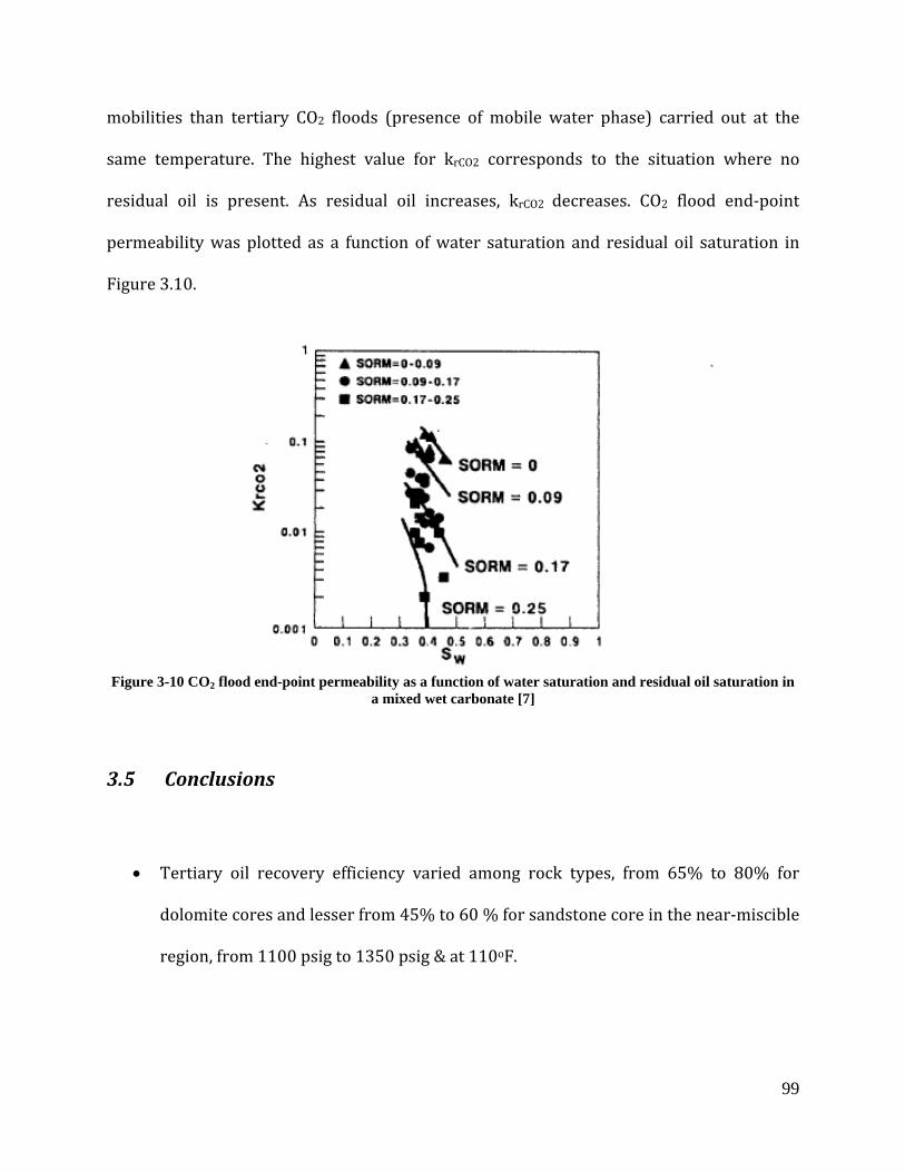
99

mobilities than tertiary CO2 floods (presence of mobile water phase) carried out at the

same temperature. The highest value for krCO2 corresponds to the situation where no

residual oil is present. As residual oil increases, krCO2 decreases. CO2 flood end-point

permeability was plotted as a function of water saturation and residual oil saturation in

Figure 3.10.

Figure 3-10 CO2 flood end-point permeability as a function of water saturation and residual oil saturation in

a mixed wet carbonate [7]

3.5 Conclusions

• Tertiary oil recovery efficiency varied among rock types, from 65% to 80% for

dolomite cores and lesser from 45% to 60 % for sandstone core in the near-miscible

region, from 1100 psig to 1350 psig & at 110oF.

100

• Recovery of more than 60% of the waterflood residual oil was obtained using

Arbuckle reservoir core when CO2 was injected at the current average reservoir

pressure 1150 psig & 110oF.

• Experimental works showed that the presence of water phase improved the relative

permeability of CO2, which coupled with the reduction of the oil viscosity reduced

the mobility ratio between the oil and CO2 and therefore the recovery efficiency was

improved

101

4 Conclusions & Recommendations

4.1 Conclusions

1. Slim tube results indicate that Arbuckle reservoirs is not a suitable candidate for

miscible CO2 flooding, since the MMP for this oil/CO2 system is 1350 psig at 110oF

whereas the operating pressure of the reservoir is 1150 psig.

2. The near miscible range is defined from 1100 psig to 1350 psig at 110oF in our

study.

3. Initial laboratory works showed that at least 80% oil recovery efficiency was

observed in slim tube tests and more than 60% of the waterflood residual oil was

obtained using Arbuckle reservoir core when CO2 was injected at the current

average reservoir pressure 1150 psig & 110oF.

4. Tertiary oil recovery efficiency varied from 65% to 80% for dolomite cores and

lesser from 45% to 60 % for sandstone core in the near-miscible region.

5. The principal oil recovery mechanism in the near-miscible range appeared to be

extraction/vaporization of hydrocarbon components from crude oil into the CO2

rich vapor phase, coupled with enhanced mobility control due to the reduction of oil

viscosity. This suggested that application of carbon dioxide in the field would

require injection and recycling of large volumes of carbon dioxide. Further study is

needed to determine if such a process is economically feasible. However the

102

prospect of recovering up to 1 billion barrels of oil from Arbuckle reservoirs offers

significant economic potential.

6. A representative phase behavior model was developed to describe the fluid

properties and fluid-fluid interaction and would be used in a compositional

simulator to evaluate the potential field application under near-miscible conditions.

4.2 Recommendations

1. Volumetric glassware read as accurately as 0.05-0.1cc, which introduces a large

uncertainty especially when the pore volumes of short cores are approximately 6-7

cc. Either long core samples should be used or volumetric glassware with smaller

divisions should be used.

2. Core flow tests were performed only once for each core and at each test condition.

Core flow tests need to be repeated to see whether the results are reproducible.

3. Wettability test should be performed for Arbuckle dolomite, Baker dolomite and

Berea sandstone. Wettability test could help explaining the difference in tertiary oil

recovery efficiencies among rock types.

4. The possible improvement of CO2 relative permeability in the presence of water

phase was used to explain for the better oil recovery efficiency seen in tertiary CO2

floods than the oil recovery efficiency seen in secondary CO2 floods. Experimental

103

measurements of CO2 relative permeability in the presence of Sorm should be

performed to verify this.

104

REFERENCES

1. Stosur, G.J., et al., Enhanced Oil Recovery in North America: Status and Prospects.

Energy Sources, Part A: Recovery, Utilization, and Environmental Effects, 1990. 12(4):

p. 429 - 437.

2. Holm, L.W., Miscibility and miscible displacement. Journal Name: J. Pet. Technol.;

(United States); Journal Volume: 38:9, 1986: p. Medium: X; Size: Pages: 817-822.

3. Green, D.W. and G.P. Willhite, Enhanced Oil Recovery. 1998: SPE.

4. Holm, L.W. and V.A. Josendal, Effect of Oil Composition on Miscible-Type

Displacement by Carbon Dioxide. 1982. 22(1): p. 87-98.

5. Metcalfe, R.S. and L. Yarborough, The Effect of Phase Equilibria on the CO2

Displacement Mechanism. 1979. 19(4): p. 242-252.

6. Klins, M.A., Carbon Dioxide Flooding Boston: International Human Resources

Development Corporation.

7. Shyeh-Yung, J.-G.J., Mechanisms of Miscible Oil Recovery: Effects of Pressure on

Miscible and Near-Miscible Displacements of Oil by Carbon Dioxide, in SPE Annual

Technical Conference and Exhibition. 1991, 1991 Copyright 1991, Society of Petroleum

Engineers Inc.: Dallas, Texas.

8. Schechter, D.S., et al., Wellman Unit CO2 Flood: Reservoir Pressure Reduction and

Flooding the Water/Oil, in SPE Annual Technical Conference and Exhibition. 1998,

Society of Petroleum Engineers: New Orleans, Louisiana.

9. Dong, M., S.S. Huang, and R. Srivastava, A Laboratory Study on Near-Miscible CO

Injection in Steelman Reservoir. 2001. 40(2).

105

10. Hadlow, R.E., Update of Industry Experience With CO2 Injection, in SPE Annual

Technical Conference and Exhibition. 1992, 1992 Copyright 1992, Society of Petroleum

Engineers Inc.: Washington, D.C.

11. Grigg, R.B., M.D. Gregory, and J.D. Purkaple, The Effect of Pressure on Improved

Oilflood Recovery from Tertiary Gas Injection. SPE Reservoir Engineering, 1997. 12(3):

p. 179-188.

12. Rahmatabadi, K.A., The role of interfacial tension in near-miscible CO2 injection, in

Chemical and Petroleum Engineering. 2006, University of Kansas: Lawrence. p. 107.

13. Ren, W. and A.M. Scurto, High-pressure phase equilibria with compressed gases (vol 78,

art no 125104, 2007). Review of Scientific Instruments, 2008. 79(2).

14. Nagarajan, N. and R.L. Robinson, Equilibrium phase compositions, phase densities, and

interfacial tensions for carbon dioxide + hydrocarbon systems. 2. Carbon dioxide + n-

decane. Journal of Chemical & Engineering Data, 1986. 31(2): p. 168-171.

15. Jennings, D.W. and R.C. Schucker, Comparison of High-Pressure Vapor−Liquid

Equilibria of Mixtures of CO2 or Propane with Nonane and C9 Alkylbenzenes. Journal of

Chemical & Engineering Data, 1996. 41(4): p. 831-838.

16. Hand, J.L. and W.V. Pinczewski, Interpretation of Swelling/Extraction Tests. SPE

Reservoir Engineering, 1990. 5(4): p. 595-600.

17. Ahosseini, A. and A. Scurto, Viscosity of Imidazolium-Based Ionic Liquids at Elevated

Pressures: Cation and Anion Effects. International Journal of Thermophysics, 2008.

29(4): p. 1222-1243.

106

18. Negahban, S. and V.J. Kremesec Jr., Development and Validation of Equation-of-State

Fluid Descriptions for CO2/Reservoir-Oil Systems. SPE Reservoir Engineering, 1992.

7(3): p. 363-368.

19. Orr Jr., F.M., et al., Laboratory Experiments To Evaluate Field Prospects for CO2

Flooding. SPE Journal of Petroleum Technology, 1982. 34(4): p. 888-898.

20. SHELTON, J.L., The Effects of Water Injection on Miscible Flooding Methods Using

Hydrocarbons and Carbon Dioxide. 1975. 15(3): p. 217-226.

21. Rathmell, J.J., F.I. Stalkup, and R.C. Hassinger, A Laboratory Investigation of Miscible

Displacement by Carbon Dioxide, in Fall Meeting of the Society of Petroleum Engineers

of AIME. 1971, 1971 Copyright 1971: New Orleans, Louisiana.

22. Wylie, P.L. and K.K. Mohanty, Effect of Wettability on Oil Recovery by Near-Miscible

Gas Injection. SPE Reservoir Evaluation & Engineering, 1999. 2(6): p. 558-564.

23. Tiffin, D.L. and W.F. Yellig, Effects of Mobile Water on Multiple-Contact Miscible Gas

Displacements. 1983. 23(3): p. 447-455.

24. Campbell, B.T. and F.M.O. Jr., Flow Visualization for CO2/Crude-Oil Displacements.

1985. 25(5): p. 665-678.

25. Stalkup, F.I., Displacement of oil by Solvent at High Water Saturation. 1970. 10(4): p.

337-348.

107

APPENDICES

Calculations of Swr, Sorw, Sorm and Swf are based on material balance. Following is an example

of how to calculate those values for Berea Sandstone at 1104 psig & 110oF.

Dead volume = 2.25 cc

Average pore volume of Berea Sandstone = 5.80 cc

Calculate residual water saturation (Swr) at the end of brine displacement test by crude oil

Assuming that the core was fully saturated with brine and the line was also completely

filled with brine, volume of brine in the core and in the line = 2.25 + 5.80 = 8.05 cc

Volume of brine collected at the end of the displacement test = 6.20 cc

Volume of brine in the core at the end of the displacement test = 8.05- 6.20 = 1.85 cc

Volume of oil in the core at the end of the displacement test = 5.80 – 1.85 = 3.95 cc

Swr = 1.85/8.50 = 0.32

So = 3.95/8.50 = 0.68

Calculate residual oil saturation (Sorw) at the end of crude oil displacement by brine

Since the line was completely filled with crude oil, volume of crude oil in the core and in the

line = 3.95 + 2.25 = 6.20 cc

108

Volume of crude oil collected at the end of the displacement test = 3.30 cc

Volume of crude oil in the core at the end of the displacement test = 6.20 – 3.30 = 2.90 cc

Volume of brine in the core at the end of the displacement test = 5.80 – 2.90 = 2.90

Sorw = 2.90/5.80 = 0.50

Sw = 2.90/5.80 = 0.50

Calculate residual oil saturation (Sorm) at the end of CO2 displacement test

Volume of crude oil prior to CO2 displacement test = 2.90 cc

Volume of crude oil collected at the end of the displacement test = 1.20 cc

Volume of oil in the core at the end of the displacement test = 2.90 – 1.20 = 1.70 cc

Sorm = 1.70/5.80 = 0.29

% Oil Recovery = (0.50-0.29)*100%/0.50 = 41.4 %

Volume of brine prior to CO2 displacement test = 2.90 + 2.25 = 5.15 cc

Volume of brine collected at the end of the displacement test = 2.90 cc

Volume of oil in the core at the end of the displacement test = 5.15 – 2.90 = 2.25 cc

Swf = 2.25/5.80 = 0.39