Embed Size (px)
Citation preview
Near-Optimal Connectivity Encoding of2-Manifold Polygon Meshes
Andrei KhodakovskyDepartment of Computer Science, Caltech
and
Pierre AlliezINRIA Sophia-Antipolis
and
Mathieu DesbrunDepartment of Computer Science, U. of So. Cal.
and
Peter SchroderDepartment of Computer Science, Caltech
Version: Februrary 23, 2002
1
Encoders for triangle mesh connectivity based on enumeration of vertex valences are among thebest reported to date. They are both simple to implement and report the best compressed file sizes fora large corpus of test models. Additionally they have recently been shown to be near-optimal sincethey realize the Tutte entropy bound for all planar triangulations.
In this paper we introduce a connectivity encoding method which extends these ideas to 2-manifold meshes consisting of faces with arbitrary degree. The encoding algorithm exploits dualityby applying valence enumeration to both the primal and dual mesh in a symmetric fashion. It gen-erates two sequences of symbols, vertex valences and face degrees, and encodes them separatelyusing two context-based arithmetic coders. This allows us to exploit vertex and/or face regularity ifpresent. When the mesh exhibits perfect face regularity (e.g., a pure triangle or quad mesh) and/orperfect vertex regularity (valence six or four respectively) the corresponding bit rate vanishes to zeroasymptotically. For triangle meshes, our technique is equivalent to earlier valence driven approaches.
We report compression results for a corpus of standard meshes. In all cases we are able to showcoding gains over earlier coders, sometimes as large as 50%. Remarkably, we even slightly gain overcoders specialized to triangle or quad meshes. A theoretical analysis reveals that our approach isnear-optimal as we achieve the Tutte entropy bound for arbitrary planar graphs of 2 bits per edge inthe worst case.
Key Words: Compression Algorithms, Connectivity Encoding, Polygon Meshes, Curves& Surfaces
1. INTRODUCTION
Encoding connectivity is an important component (next to geometry coding) of allsurface compression algorithms to date. This is true for single rate and progressive codersand independent of the surface primitive,e.g., piecewise linear, NURBS, subdivision, ormultiresolution patches.
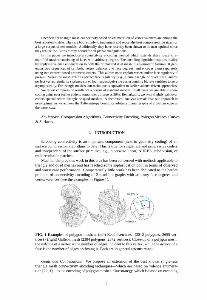
Much of the previous work in this area has been concerned with methods applicable totriangle and quad meshes and has reached some sophistication both in terms of observedand worst case performance. Comparatively little work has been dedicated to the harderproblem of connectivity encoding of 2-manifold graphs with arbitrary face degrees andvertex valences (see the examples in Figure1).
Degree 5
Valence 4
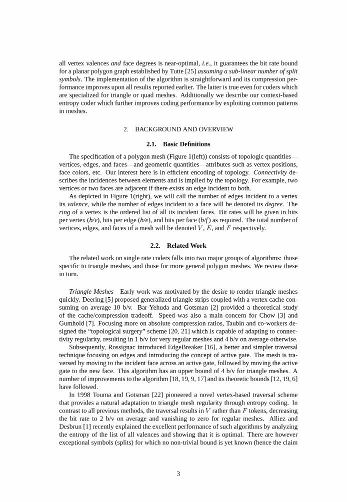
FIG. 1 Examples of polygon meshes: (left) Beethoven mesh (2812 polygons, 2655 ver-tices) - (right) Galleon mesh (2384 polygons, 2372 vertices). Close-up of a polygon mesh:thevalenceof a vertex is the number of edges incident to this vertex, while thedegreeof aface is the number of edges enclosing it. Both are in general unconstrained.
Goals and Contributions We propose an extension of the best known single-ratetriangle mesh connectivity encoding techniques—which are based on valence enumera-tion [22, 1]—to the encoding of polygon meshes. Our strategy, which is based on encoding
2
all vertex valencesand face degrees is near-optimal,i.e., it guarantees the bit rate boundfor a planar polygon graph established by Tutte [25] assuming a sub-linear number of splitsymbols. The implementation of the algorithm is straightforward and its compression per-formance improves upon all results reported earlier. The latter is true even for coders whichare specialized for triangle or quad meshes. Additionally we describe our context-basedentropy coder which further improves coding performance by exploiting common patternsin meshes.
2. BACKGROUND AND OVERVIEW
2.1. Basic Definitions
The specification of a polygon mesh (Figure1(left)) consists of topologic quantities—vertices, edges, and faces—and geometric quantities—attributes such as vertex positions,face colors, etc. Our interest here is in efficient encoding of topology.Connectivityde-scribes the incidences between elements and is implied by the topology. For example, twovertices or two faces are adjacent if there exists an edge incident to both.
As depicted in Figure1(right), we will call the number of edges incident to a vertexits valence, while the number of edges incident to a face will be denoted itsdegree. Thering of a vertex is the ordered list of all its incident faces. Bit rates will be given in bitsper vertex (b/v), bits per edge (b/e), and bits per face (b/f) as required. The total number ofvertices, edges, and faces of a mesh will be denotedV , E, andF respectively.
2.2. Related Work
The related work on single rate coders falls into two major groups of algorithms: thosespecific to triangle meshes, and those for more general polygon meshes. We review thesein turn.
Triangle Meshes Early work was motivated by the desire to render triangle meshesquickly. Deering [5] proposed generalized triangle strips coupled with a vertex cache con-suming on average 10 b/v. Bar-Yehuda and Gotsman [2] provided a theoretical studyof the cache/compression tradeoff. Speed was also a main concern for Chow [3] andGumhold [7]. Focusing more on absolute compression ratios, Taubin and co-workers de-signed the “topological surgery” scheme [20, 21] which is capable of adapting to connec-tivity regularity, resulting in 1 b/v for very regular meshes and 4 b/v on average otherwise.
Subsequently, Rossignac introduced EdgeBreaker [16], a better and simpler traversaltechnique focusing on edges and introducing the concept of active gate. The mesh is tra-versed by moving to the incident face across an active gate, followed by moving the activegate to the new face. This algorithm has an upper bound of 4 b/v for triangle meshes. Anumber of improvements to the algorithm [18, 19, 9, 17] and its theoretic bounds [12, 19, 6]have followed.
In 1998 Touma and Gotsman [22] pioneered a novel vertex-based traversal schemethat provides a natural adaptation to triangle mesh regularity through entropy coding. Incontrast to all previous methods, the traversal results inV rather thanF tokens, decreasingthe bit rate to 2 b/v on average and vanishing to zero for regular meshes. Alliez andDesbrun [1] recently explained the excellent performance of such algorithms by analyzingthe entropy of the list of all valences and showing that it is optimal. There are howeverexceptional symbols (splits) for which no non-trivial bound is yet known (hence the claim
3
of “near”-optimality). As a practical solution they proposed an adaptive traversal controlheuristic which reduces the number of splits to get closer to the optimal bit rate.
Arbitrary Polygon Meshes Given that a polygon mesh with the same number of ver-tices contains less edges than a triangle mesh it should be possible to encode it with fewerbits. However, initial attempts to compress general graphs [23, 11] led to rates of around9 b/v. These methods are based on building interlocking spanning trees for vertices andfaces. Consequently, the number of edges becomes the natural measure of planar graphsize, in turn governing the encoding size. Chuanget al. [4] later described a more com-pact encoding via canonical ordering and multiple parentheses. They state that any simple3-connected plane graph can be encoded using at most1.5 log2(3)E + 3 ' 2.377 bits peredge.
Li and Kuo [15] pioneered a dual approach that traverses the edges of the dual meshand outputs a variable length sequence of symbols based on the type of a visited edge. Thefinal sequence is then encoded using a context based entropy encoder.
Isenburg and Snoeyink encoded the connectivity of polygon meshes along with theirproperties in a method calledFace Fixer[10]. This algorithm is gate-based and generalizesthe EdgeBreaker algorithm while adding the notion of a face degree. A complete traversalof the mesh is organized through successive gate labeling along an active boundary loop.As in [22, 16] both the encoder and decoder need a stack of boundary loops. Seven distinctlabels Fn, R, L, S, E, Hn and Mi,k,l are used in order to describe the way tofix faces or holestogether while traversing the current active gate. The labels Fn correspond to face degreesand are limited to the range[3 − 5] thanks to an additional special symbol Fc. Since thefinal sequence of symbols exhibits strong correlation the authors used an order-3 arithmeticcoder. Kinget al. [13] and Kronrod and Gotsman [14] also generalized the EdgeBreakermethod to arbitrary polygon meshes. For the former quad meshes are encoded with3 b/vand for the latter quad meshes are encoded with3.5 b/v and quadrilateral meshes containinga minority of triangles with4 b/v. However, none of these polygon mesh encoders comeclose to the bit rates of any of the best, specialized encoders [22, 1] when applied to trianglemeshes.
2.3. Key Concept: Duality
In addition to the previous work analysis, we make the following observation. Con-sider an arbitrary 2-manifold triangle graphM. Its dual graphM, in which faces arerepresented as dual vertices and vertices become dual faces (see Figure2), should havethe same connectivity entropy: dualization neither adds nor removes information. The va-lences ofM are now all equal to3, while the face degrees take on the same values as thevertex valences ofM. Since a list of all3s has zero entropy, just encoding the list of de-grees ofM would lead to the same bit rate as found for the valences ofM. Conversely, ifa polygon mesh has only valence-3 vertices, then its dual would be a triangle mesh. Henceits entropy should be equal to the entropy of the list of its degrees.
The above observation leads us to the key concept of this paper: our compressionalgorithm should bedual, in the sense that both a mesh and its dual get encoded with thesame number of bits. As a direct consequence, the encoding process should be symmetricin the coding of valences and degrees. In fact, we will show in the Appendix that encodingeach separately realizes the enumeration bound of Tutte. A second direct consequence isthat the bit rate of a mesh should be measured in b/e, since the number of edges is the onlyvariable not changing during a graph dualization. However, for purposes of comparisonwith earlier work we will report comparative results in b/v in Section4.
4
3
5
3
5
Primal mesh Dualization Dual mesh
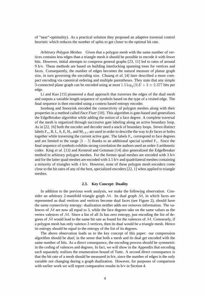
FIG. 2 Left: a polygon mesh with highlighted faces of degree 3 and 5. Middle: the dualmesh is built by placing one node in each original face and connecting them through eachedge incident to two original faces. Right: the dual mesh now contains correspondingvertices of valence 3 and 5.
Note: While this paper was in review, we learned about a similar approach concurrentlydeveloped in independent work by Isenburg [8]. It also exploits the idea of dual meshentropy and lends additional support to the usefulness of this approach. We refer the inter-ested reader to [8] for additional details.
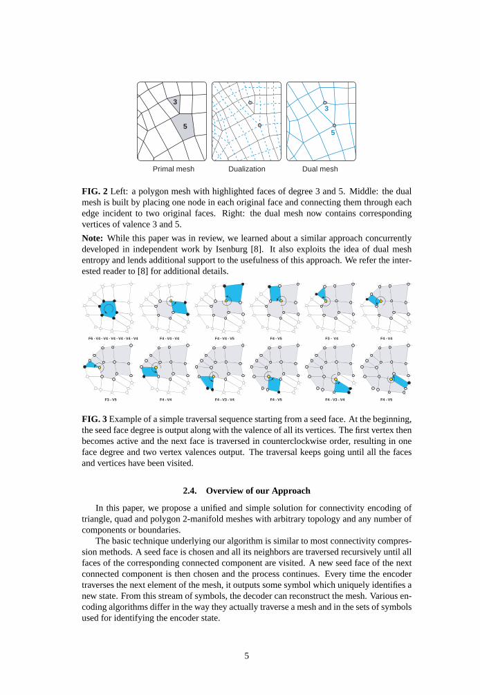
F6 - V4 - V4 - V4 - V4 - V4 - V4 F4 - V4 - V4 F4 - V4 - V5 F4 - V5 F3 - V4 F4 - V4
F3 - V5 F4 - V4 F4 - V3 - V4 F4 - V5 F4 - V3 - V4 F4 - V5
FIG. 3 Example of a simple traversal sequence starting from a seed face. At the beginning,the seed face degree is output along with the valence of all its vertices. The first vertex thenbecomes active and the next face is traversed in counterclockwise order, resulting in oneface degree and two vertex valences output. The traversal keeps going until all the facesand vertices have been visited.
2.4. Overview of our Approach
In this paper, we propose a unified and simple solution for connectivity encoding oftriangle, quad and polygon 2-manifold meshes with arbitrary topology and any number ofcomponents or boundaries.
The basic technique underlying our algorithm is similar to most connectivity compres-sion methods. A seed face is chosen and all its neighbors are traversed recursively until allfaces of the corresponding connected component are visited. A new seed face of the nextconnected component is then chosen and the process continues. Every time the encodertraverses the next element of the mesh, it outputs some symbol which uniquely identifies anew state. From this stream of symbols, the decoder can reconstruct the mesh. Various en-coding algorithms differ in the way they actually traverse a mesh and in the sets of symbolsused for identifying the encoder state.
5
As we have seen in the previous work section, a generalization of the gate-based ap-proach to arbitrary polygon meshes was suggested in [10]. In the present paper we proposea generalization of the second, vertex-based approach. Because of the duality properties ofour approach, it may equivalently be viewed as a face-based approach. We use two sets ofsymbols to encode vertex valences and face degrees. At any given moment both encoderand decoder will know which type of symbol (face or vertex) they are dealing with. Con-sequently, if the input mesh contains only faces of fixed degree (all triangles or all quads,for example), the corresponding stream will be compressed to near zero b/f by an entropycoder leaving only a vertex valence stream. Conversely, if the mesh has faces of varyingdegrees, but all vertices have the same valence, we get a zero entropy vertex stream. Notethat the FaceFixer algorithm also uses face degrees, so it can take advantage of a meshwith uniform face degrees, but not of one with uniform vertex valences. The shark modelexemplifies such a case (see Table2).
3. ENCODING ALGORITHM
In this section we give a complete, yet informal description of our algorithm, includingthe data structures needed. Pseudo code giving exact details is included in the Appendix.We also discuss the optimality of our approach, and show that encoding both the valenceand degree lists exactly matches the worst-case entropy for a planar graph as establishedby Tutte [25].
Data Structures We maintain only vertex and face data structures explicitly. Verticesstore their valence and references to all incident faces in counterclockwise order. Similarly,a face stores its degree and references to all incident vertices in counterclockwise order.Vertices as well as faces go through a sequence of states:empty, active, andcomplete. Atany given time at most one face is active, but there may be multiple vertices active. Theseare held in theactive vertex queue. When a face is processed—moved from empty to activeto complete states—all its vertices, which are not yet active, are activated through insertioninto the active vertex queue. Consequently, each active vertex has at least one completeincident face. As soon as all the faces incident to a vertex have become complete, the vertexchanges its state to complete and is removed from the queue. Thus, the active vertex queuerepresents theboundarybetween the part of the mesh which has already been traversedand the part as yet to be visited.
3.1. Traversal Strategy
Initialization step We start the mesh traversal by picking an initial seed face. Theencoder outputs the degree of this face, followed by the valences of all the vertices incidentto this face in counterclockwise order. These vertices are added to the queue. Conversely,the decoder receives the seed face degree and creates a corresponding face. It then fills allthe slots for the incident vertices, moving them from the empty to active state,i.e., entersthem into its queue. In this way encoder and decoder maintain matching states.
Completing the verticesThe traversal continues by removing the highest priority ac-tive vertex from the queue and making it thecurrentvertex. We will discuss heuristics forqueue priority assignment in Section3.3.
The algorithm proceeds counterclockwise around the active vertex, skipping all faceswhich have already been completed. Recall that at least one face is completed and at least
6
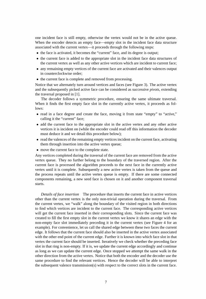
one incident face is still empty, otherwise the vertex would not be in the active queue.When the encoder detects an empty face—empty slot in the incident face data structureassociated with the current vertex—it proceeds through the following steps:
• the face is activated, it becomes the “current” face, and its degree is output;
• the current face is added to the appropriate slot in the incident face data structures ofthe current vertex as well as any other active vertices which are incident to current face;
• any remaining empty vertices of the current face are activated and their valences outputin counterclockwise order;
• the current face is complete and removed from processing.
Notice that we alternately turn around vertices and faces (see Figure3). The active vertexand the subsequently picked active face can be considered as successivepivots, extendingthe traversal proposed in [1].
The decoder follows a symmetric procedure, ensuring the same ultimate traversal.When it finds the first empty face slot in the currently active vertex, it proceeds as fol-lows:
• read in a face degree and create the face, moving it from state “empty” to “active,”calling it the “current” face;
• add the current face to the appropriate slot in the active vertex and any other activevertices it is incident on (while the encoder could read off this information the decodermust deduce it and we detail this procedure below);
• read the valences of the remaining empty vertices incident on the current face, activatingthem through insertion into the active vertex queue;
• move the current face to the complete state.
Any vertices completed during the traversal of the current face are removed from the activevertex queue. They no further belong to the boundary of the traversed region. After thecurrent face is processed the algorithm proceeds to the next face in the currently activevertex until it is complete. Subsequently a new active vertex is taken from the queue andthe process repeats until the active vertex queue is empty. If there are some connectedcomponents remaining, a new seed face is chosen on it and another component traversalstarts.
Details of face insertion The procedure that inserts the current face in active verticesother than the current vertex is the only non-trivial operation during the traversal. Fromthe current vertex, we “walk” along the boundary of the visited region in both directionsto find which vertices are incident to the current face. The corresponding active verticeswill get the current face inserted in their corresponding slots. Since the current face wascreated to fill the first empty slot in the current vertex we know it shares an edge with thenon-empty face slot immediately preceding it in the current vertex (see Figure4 for anexample). For convenience, let us call the shared edge between these two faces the currentedge. It follows that the current face should also be inserted in the active vertex associatedwith the other end point of the current edge. Further it is known into which face slot in thatvertex the current face should be inserted. Iteratively we check whether the preceding faceslot in that ring is non-empty. If it is, we update the current edge accordingly and continueas long as we can update the current edge. Once stopped we attempt the same walk in theother direction from the active vertex. Notice that both the encoder and the decoder use thesame procedure to find the relevant vertices. Hence the decoder will be able to interpretthe subsequent valence transmission(s) with respect to the correct slots in the current face.
7
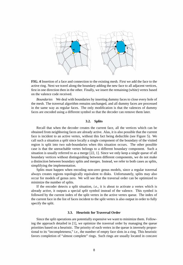
FIG. 4 Insertion of a face and connection to the existing mesh. First we add the face to theactive ring. Next we travel along the boundary adding the new face to all adjacent vertices,first in one direction then in the other. Finally, we insert the remaining (white) vertex basedon the valence code received.
Boundaries We deal with boundaries by inserting dummy faces to close every hole ofthe mesh. The traversal algorithm remains unchanged, and all dummy faces are processedin the same way as regular faces. The only modification is that the valences of dummyfaces are encoded using a different symbol so that the decoder can remove them later.
3.2. Splits
Recall that when the decoder creates the current face, all the vertices which can beobtained from neighboring faces are already active. Alas, it is also possible that the currentface is incident to an active vertex, without this fact being deducible (see Figure5). Wecall such a situation asplit since locally a single component of the boundary of the visitedregion is split into two sub-boundaries when this situation occurs. The other possiblecase is that the unreachable vertex belongs to a different boundary component. Such asituation is usually referred to as a merge [22, 1]. Since we only keep a single queue of allboundary vertices without distinguishing between different components, we do not makea distinction between boundary splits and merges. Instead, we refer to both cases as splits,simplifying the implementation.
Splits must happen when encoding non-zero genus models, since a regular traversalalways creates regions topologically equivalent to disks. Unfortunately, splits may alsooccur for models of genus zero. We will see that the traversal order can be optimized tominimize the number of splits.
If the encoder detects a split situation,i.e., it is about to activate a vertex which isalready active, it outputs a specialsplit symbol instead of the valence. This symbol isfollowed by the current index of the split vertex in the active vertex queue. The index ofthe current face in the list of faces incident to the split vertex is also output in order to fullyspecify the split.
3.3. Heuristic for Traversal Order
Since the split operations are potentially expensive we want to minimize them. Follow-ing the approach detailed in [1], we optimize the traversal order by managing the queuepriorities based on a heuristic. The priority of each vertex in the queue is inversely propor-tional to its “incompleteness,”i.e., the number of empty face slots in a ring. This heuristicfavors completion of “almost complete” rings. Such rings are usually located in concave
8
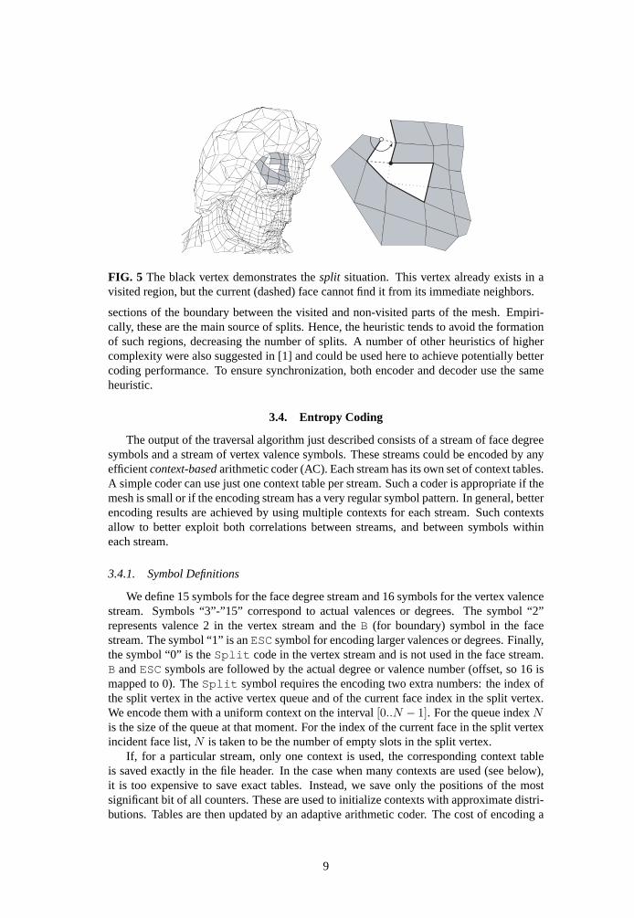
FIG. 5 The black vertex demonstrates thesplit situation. This vertex already exists in avisited region, but the current (dashed) face cannot find it from its immediate neighbors.
sections of the boundary between the visited and non-visited parts of the mesh. Empiri-cally, these are the main source of splits. Hence, the heuristic tends to avoid the formationof such regions, decreasing the number of splits. A number of other heuristics of highercomplexity were also suggested in [1] and could be used here to achieve potentially bettercoding performance. To ensure synchronization, both encoder and decoder use the sameheuristic.
3.4. Entropy Coding
The output of the traversal algorithm just described consists of a stream of face degreesymbols and a stream of vertex valence symbols. These streams could be encoded by anyefficientcontext-basedarithmetic coder (AC). Each stream has its own set of context tables.A simple coder can use just one context table per stream. Such a coder is appropriate if themesh is small or if the encoding stream has a very regular symbol pattern. In general, betterencoding results are achieved by using multiple contexts for each stream. Such contextsallow to better exploit both correlations between streams, and between symbols withineach stream.
3.4.1. Symbol Definitions
We define 15 symbols for the face degree stream and 16 symbols for the vertex valencestream. Symbols “3”-”15” correspond to actual valences or degrees. The symbol “2”represents valence 2 in the vertex stream and theB (for boundary) symbol in the facestream. The symbol “1” is anESCsymbol for encoding larger valences or degrees. Finally,the symbol “0” is theSplit code in the vertex stream and is not used in the face stream.B andESCsymbols are followed by the actual degree or valence number (offset, so 16 ismapped to 0). TheSplit symbol requires the encoding two extra numbers: the index ofthe split vertex in the active vertex queue and of the current face index in the split vertex.We encode them with a uniform context on the interval[0..N − 1]. For the queue indexNis the size of the queue at that moment. For the index of the current face in the split vertexincident face list,N is taken to be the number of empty slots in the split vertex.
If, for a particular stream, only one context is used, the corresponding context tableis saved exactly in the file header. In the case when many contexts are used (see below),it is too expensive to save exact tables. Instead, we save only the positions of the mostsignificant bit of all counters. These are used to initialize contexts with approximate distri-butions. Tables are then updated by an adaptive arithmetic coder. The cost of encoding a
9
non-empty table is 2-3 bytes on average compared to 10-12 bytes for encoding of an exacttable.
3.4.2. Our Statistical Model
The face and vertex streams are encoded using multiple contexts. The appropriate con-text is chosen based on already-known information about neighboring faces and vertices.This approach is different from using a higher-order arithmetic coder which uses a numberof previously processed symbols to define the new context. The latter approach is less ad-vantageous, since some of the previous symbols may correspond to faces or vertices whichare not relevant to the current symbol.
Face degrees The context for a face degree symbolF is determined by the degree ofthe previous faceFp in the same active ring and the sumVav of valences of the vertices onthe edge between the current and the previous faces.
In particular, we separately consider most common degrees 3, 4, 5. IfFp has someother degree we encode the symbolF with a default context. The same default context isused when there is no previous face. We use three different contexts for each of degrees 3and 4 and just one context for a less common degree 5. We decide between three possiblecontexts depending onVav < Vcrit, Vav = Vcrit, Vav > Vcrit whereVcrit = 12 if Fp is atriangle andVcrit = 8 if Fp is a quad.
Vertex valences are encoded with 8 contexts in a similar way to face degrees. Thecontext for the vertexV is determined by the degree of the faceF which contains thisvertex and the sumVav of valences of all know vertices in that face.
We use three contexts ifF is a triangle or quad, one context for degree 5 and onecontext for other degrees. IfF is a triangle or a quad we distinguish between three possiblecontexts depending onVav < Nv · Vcrit, Vav = Nv · Vcrit, or Vav > Nv · Vcrit, whereNv
is a number of known vertices andVcrit is 6 for triangles and 4 for quads.
Discussion The motivation for using such contexts is that the average valence of ver-tices in quad and triangle regions are different. Therefore, there is a correlation between thevertex or face symbol to encode and the average valence of known neighboring vertices.
We have found the above heuristics to generally improve the coding of meshes. Wehave experimented our technique on the large SNHC database, and on average, a gain of13% is observed when we use our simple statistical model over a direct encoding (slightlyworse bitrates are obtained only for small meshes). We also show in Table1 that using onlycontexts based on valences or degrees is consistently worse than our mixed strategy on this3D database. Although one could adjust this strategy to perform better on a given corpusof meshes, our choice seems a good compromise for the typical meshes used in graphics.
3.5. Optimality
Alliez and Desbrun [1] have recently proven that the list of valences of a triangle meshis an exact entropy measure of connectivity. The worst case scenario fits the theoreticalresults of Tutte [24] of log2(256/27) ≈ 3.24 bits per vertex, while regularity in valenceleads to almost zero entropy. In AppendixA we prove, using a similar approach, that theentropy of the two lists of valences and degrees also matches the counting results of Tuttefor general, 3-connected graphs [25]. This proves the “near-optimality” of our approach:under the assumption that only a sub-linear number of splits is produced during encoding,
10
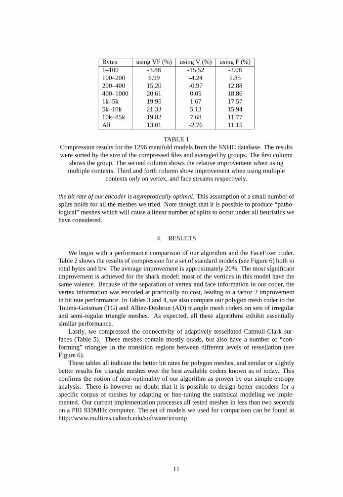
Bytes using VF (%) using V (%) using F (%)1–100 -3.88 -15.52 -3.08100–200 6.99 -4.24 5.85200–400 15.20 -0.97 12.88400–1000 20.61 0.05 18.861k–5k 19.95 1.67 17.575k–10k 21.33 5.13 15.9410k–85k 19.82 7.68 11.77All 13.01 -2.76 11.15
TABLE 1Compression results for the 1296 manifold models from the SNHC database. The resultswere sorted by the size of the compressed files and averaged by groups. The first column
shows the group. The second column shows the relative improvement when usingmultiple contexts. Third and forth column show improvement when using multiple
contextsonlyon vertex, and face streams respectively.
the bit rate of our encoder is asymptotically optimal. This assumption of a small number ofsplits holds for all the meshes we tried. Note though that it is possible to produce “patho-logical” meshes which will cause a linear number of splits to occur under all heuristics wehave considered.
4. RESULTS
We begin with a performance comparison of our algorithm and the FaceFixer coder.Table2 shows the results of compression for a set of standard models (see Figure6) both intotal bytes and b/v. The average improvement is approximately 20%. The most significantimprovement is achieved for the shark model: most of the vertices in this model have thesame valence. Because of the separation of vertex and face information in our coder, thevertex information was encoded at practically no cost, leading to a factor2 improvementin bit rate performance. In Tables3 and4, we also compare our polygon mesh coder to theTouma-Gotsman (TG) and Alliez-Desbrun (AD) triangle mesh coders on sets of irregularand semi-regular triangle meshes. As expected, all these algorithms exhibit essentiallysimilar performance.
Lastly, we compressed the connectivity of adaptively tessellated Catmull-Clark sur-faces (Table5). These meshes contain mostly quads, but also have a number of “con-forming” triangles in the transition regions between different levels of tessellation (seeFigure6).
These tables all indicate the better bit rates for polygon meshes, and similar or slightlybetter results for triangle meshes over the best available coders known as of today. Thisconfirms the notion of near-optimality of our algorithm as proven by our simple entropyanalysis. There is however no doubt that it is possible to design better encoders for aspecific corpus of meshes by adapting or fine-tuning the statistical modeling we imple-mented. Our current implementation processes all tested meshes in less than two secondson a PIII 933MHz computer. The set of models we used for comparison can be found athttp://www.multires.caltech.edu/software/ircomp
11
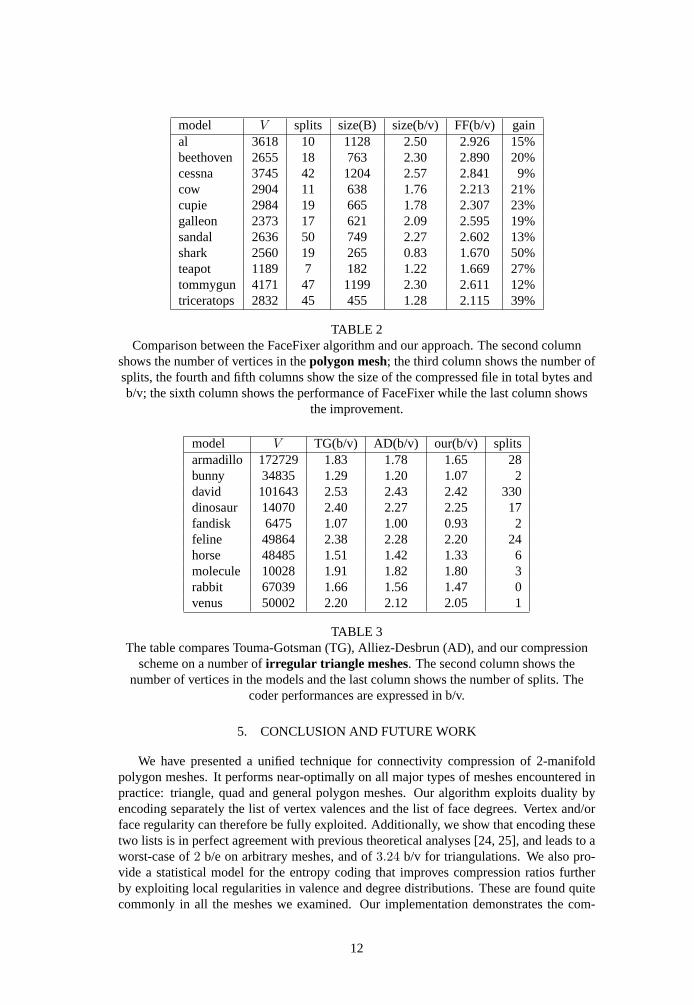
model V splits size(B) size(b/v) FF(b/v) gainal 3618 10 1128 2.50 2.926 15%beethoven 2655 18 763 2.30 2.890 20%cessna 3745 42 1204 2.57 2.841 9%cow 2904 11 638 1.76 2.213 21%cupie 2984 19 665 1.78 2.307 23%galleon 2373 17 621 2.09 2.595 19%sandal 2636 50 749 2.27 2.602 13%shark 2560 19 265 0.83 1.670 50%teapot 1189 7 182 1.22 1.669 27%tommygun 4171 47 1199 2.30 2.611 12%triceratops 2832 45 455 1.28 2.115 39%
TABLE 2Comparison between the FaceFixer algorithm and our approach. The second column
shows the number of vertices in thepolygon mesh; the third column shows the number ofsplits, the fourth and fifth columns show the size of the compressed file in total bytes andb/v; the sixth column shows the performance of FaceFixer while the last column shows
the improvement.
model V TG(b/v) AD(b/v) our(b/v) splitsarmadillo 172729 1.83 1.78 1.65 28bunny 34835 1.29 1.20 1.07 2david 101643 2.53 2.43 2.42 330dinosaur 14070 2.40 2.27 2.25 17fandisk 6475 1.07 1.00 0.93 2feline 49864 2.38 2.28 2.20 24horse 48485 1.51 1.42 1.33 6molecule 10028 1.91 1.82 1.80 3rabbit 67039 1.66 1.56 1.47 0venus 50002 2.20 2.12 2.05 1
TABLE 3The table compares Touma-Gotsman (TG), Alliez-Desbrun (AD), and our compression
scheme on a number ofirregular triangle meshes. The second column shows thenumber of vertices in the models and the last column shows the number of splits. The
coder performances are expressed in b/v.
5. CONCLUSION AND FUTURE WORK
We have presented a unified technique for connectivity compression of 2-manifoldpolygon meshes. It performs near-optimally on all major types of meshes encountered inpractice: triangle, quad and general polygon meshes. Our algorithm exploits duality byencoding separately the list of vertex valences and the list of face degrees. Vertex and/orface regularity can therefore be fully exploited. Additionally, we show that encoding thesetwo lists is in perfect agreement with previous theoretical analyses [24, 25], and leads to aworst-case of2 b/e on arbitrary meshes, and of3.24 b/v for triangulations. We also pro-vide a statistical model for the entropy coding that improves compression ratios furtherby exploiting local regularities in valence and degree distributions. These are found quitecommonly in all the meshes we examined. Our implementation demonstrates the com-
12
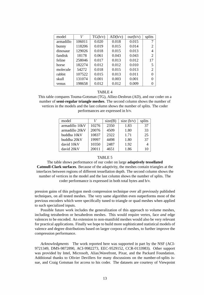
model V TG(b/v) AD(b/v) our(b/v) splitsarmadillo 106011 0.020 0.018 0.015 7bunny 118206 0.019 0.015 0.014 2dinosaur 129026 0.018 0.015 0.013 4fandisk 18178 0.061 0.043 0.043 2feline 258046 0.017 0.013 0.012 17horse 182274 0.012 0.012 0.010 5molecule 54272 0.018 0.015 0.013 2rabbit 107522 0.015 0.013 0.011 0skull 131074 0.001 0.003 0.001 0venus 198658 0.012 0.012 0.009 0
TABLE 4This table compares Touma-Gotsman (TG), Alliez-Desbrun (AD), and our coder on anumber ofsemi-regular triangle meshes. The second column shows the number of
vertices in the models and the last column shows the number of splits. The coderperformances are expressed in b/v.
model V size(B) size (b/v) splitsarmadillo 10kV 10276 2350 1.83 37armadillo 20kV 20076 4509 1.80 33buddha 10kV 10837 2322 1.71 25buddha 20kV 19997 4498 1.80 37david 10kV 10350 2487 1.92 4david 20kV 20011 4651 1.86 10
TABLE 5The table shows performance of our coder on largeadaptively tessellated
Catmull-Clark surfaces. Because of the adaptivity, the meshes contain triangles at theinterfaces between regions of different tessellation depth. The second column shows the
number of vertices in the model and the last column shows the number of splits. Thecoder performance is expressed in both total bytes and b/v.
pression gains of this polygon mesh compression technique over all previously publishedtechniques, on all tested meshes. The very same algorithm even outperforms most of theprevious encoders which were specifically tuned to triangle or quad meshes when appliedto such specialized inputs.
Possible future work includes the generalization of this approach to volume meshes,including tetrahedron or hexahedron meshes. This would require vertex, faceand edgevalences to be encoded. An extension to non-manifold meshes would also be very relevantfor practical applications. Finally we hope to build more sophisticated statistical models ofvalence and degree distributions based on larger corpora of meshes, to further improve thecompression performance.
AcknowledgmentsThe work reported here was supported in part by the NSF (ACI-9721349, DMS-9872890, ACI-9982273, EEC-9529152, CCR-0133983). Other supportwas provided by Intel, Microsoft, Alias|Wavefront, Pixar, and the Packard Foundation.Additional thanks to Olivier Devillers for many discussions on the number-of-splits is-sue, and Craig Gotsman for access to his coder. The datasets are courtesy of Viewpoint
13
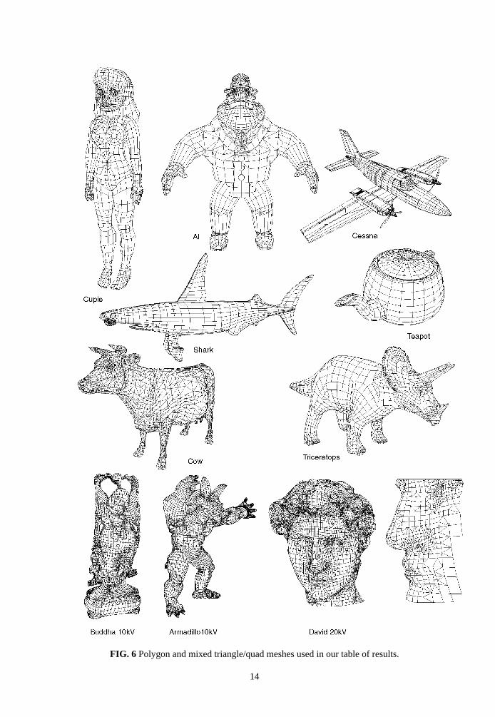
FIG. 6 Polygon and mixed triangle/quad meshes used in our table of results.
14
Datalabs, Martin Isenburg, Digital Michelangelo Project, Stanford University, Cyberware,Headus, Hugues Hoppe, and The Scripps Research Institute.
REFERENCES
[1] ALLIEZ , P., AND DESBRUN, M. Valence-Driven Connectivity Encoding of 3DMeshes. In Eurographics 2001 Conference Proceedings(Sept. 2001), pp. 480–489.
[2] BAR-YEHUDA, R., AND GOTSMAN, C. Time/space Tradeoffs for Polygon MeshRendering. ACM Transactions on Graphics 15(2)(1996), 141–152.
[3] CHOW, M. Optimized Geometry Compression for Real-Time Rendering. In Visual-ization 97 Conference Proceedings(1997), pp. 347–354.
[4] CHUANG, R. C.-N., GARG, A., HE, X., KAO, M.-Y., AND LU, H.-I. CompactEncodings of Planar Graphs via Canonical Orderings and Multiple Parentheses. InAutomata, Languages and Programming(1998), pp. 118–129.
[5] DEERING, M. Geometry Compression. InACM SIGGRAPH 98 Conference Pro-ceedings(1995), pp. 13–20.
[6] GUMHOLD , S. New Bounds on the Encoding of Planar Triangulations. Tech. Rep.WSI-2000-1, Wilhelm Schickard Institute for Computer Science, Tubingen, March2000.
[7] GUMHOLD , S., AND STRASSER, W. Real Time Compression of Triangle MeshConnectivity. InSIGGRAPH 98 Conference Proceedings(1998), pp. 133–140.
[8] ISENBURG, M. Compressing Polygon Mesh Connectivity with Degree Duality Pre-diction. In to appear in Graphics Interface(27-29 May 2002).
[9] ISENBURG, M., AND SNOEYINK , J. Spirale Reversi: Reverse Decoding of Edge-Breaker Encoding. 12th Canadian Conference on Computational Geometry(2000),247–256.
[10] ISENBURG, M., AND SNOEYINK , J.Face Fixer: Compressing Polygon Meshes WithProperties. In ACM SIGGRAPH 2000 Conference Proceedings(2000), pp. 263–270.
[11] KEELER, AND WESTBROOK. Short Encodings of Planar Graphs and Maps.DAMATH: Discrete Applied Mathematics and Combinatorial Operations Researchand Computer Science 58(1995).
[12] K ING, D., AND ROSSIGNAC, J. Guaranteed 3.67V bit Encoding of Planar TriangleGraphs. 11th Canadian Conference on Computational Geometry(1999), 146–149.
[13] K ING, D., ROSSIGNAC, J., AND SZMCZAK , A. Connectivity Compression for Ir-regular Quadrilateral Meshes. Tech. Rep. TR–99–36, GVU, Georgia Tech, 1999.
[14] KRONROD, B., AND GOTSMAN, C. Efficient Coding of Non-Triangular Meshes. InPacific Graphics 2000 Conference Proceedings(october 2000).
[15] L I , J., AND KUO, C.-C. J. Mesh connectivity coding by the dual graph approach,July 1998. MPEG98 Contribution Document No. M3530, Dublin, Ireland.
15
[16] ROSSIGNAC, J. EdgeBreaker : Connectivity Compression for Triangle Meshes.IEEE Transactions on Visualization and Computer Graphics(1999), 47–61.
[17] ROSSIGNAC, J., SAFONOVA, A., AND SZYMCZAK , A. 3D Compression MadeSimple: Edgebreaker on a Corner-Table, 2001.
[18] ROSSIGNAC, J., AND SZYMCZAK , A. Wrap&Zip Decompression of the Connec-tivity of Triangle Meshes Compressed with EdgeBreaker. Journal of ComputationalGeometry, Theory and Applications 14(november 1999), 119–135.
[19] SZYMCZAK , A., K ING, D., AND ROSSIGNAC, J. An EdgeBreaker-based EfficientCompression Scheme for Regular Meshes. 12th Canadian Conference on Computa-tional Geometry(2000), 257–265.
[20] TAUBIN , G., HORN, W., LAZARUS, F., AND ROSSIGNAC, J. Geometry Coding andVRML. Proceedings of the IEEE 96(6)(1998), 1228–1243.
[21] TAUBIN , G., AND ROSSIGNAC, J. Geometric Compression Through TopologicalSurgery. ACM Transactions on Graphics 17, 2 (April 1998), 84–115.
[22] TOUMA , C., AND GOTSMAN, C. Triangle Mesh Compression. Graphics Interface98 Conference Proceedings(june 1998), 26–34.
[23] TURAN, G. Succinct representations of graphs.Discrete Applied Mathematics 8(1984), 289–294.
[24] TUTTE, W. A Census of Planar Triangulations.Canadian Journal of Mathematics14 (1962), 21–38.
[25] TUTTE, W. A Census of Planar Maps.Canadian Journal of Mathematics 15(1963),249–271.
16
APPENDIX A: ENTROPY ANALYSIS
Consider a 2-manifold polygon meshM with V vertices,E edges, andF faces, andthe following standard assumptions on the mesh:
• it has no boundary,i.e., every edge has two incident faces;
• it is topologically equivalent to a sphere,i.e., has genus zero;
• it has only one connected component.
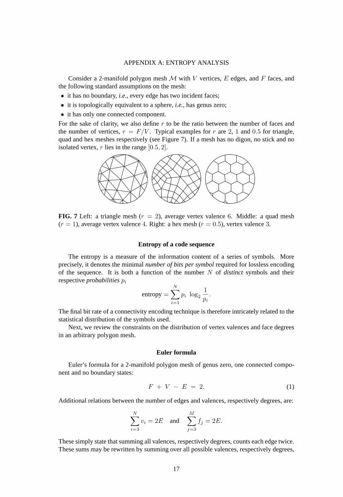
For the sake of clarity, we also definer to be the ratio between the number of faces andthe number of vertices,r = F/V . Typical examples forr are2, 1 and0.5 for triangle,quad and hex meshes respectively (see Figure7). If a mesh has no digon, no stick and noisolated vertex,r lies in the range[0.5, 2].
FIG. 7 Left: a triangle mesh (r = 2), average vertex valence6. Middle: a quad mesh(r = 1), average vertex valence4. Right: a hex mesh (r = 0.5), vertex valence3.
Entropy of a code sequence
The entropy is a measure of the information content of a series of symbols. Moreprecisely, it denotes the minimalnumber of bits per symbolrequired for lossless encodingof the sequence. It is both a function of the numberN of distinct symbols and theirrespectiveprobabilitiespi
entropy=N∑
i=1
pi log2
1pi
.
The final bit rate of a connectivity encoding technique is therefore intricately related to thestatistical distribution of the symbols used.
Next, we review the constraints on the distribution of vertex valences and face degreesin an arbitrary polygon mesh.
Euler formula
Euler’s formula for a 2-manifold polygon mesh of genus zero, one connected compo-nent and no boundary states:
F + V − E = 2. (1)
Additional relations between the number of edges and valences, respectively degrees, are:
N∑i=3
vi = 2E andM∑
j=3
fj = 2E.
These simply state that summing all valences, respectively degrees, counts each edge twice.These sums may be rewritten by summing over all possible valences, respectively degrees,
17
the number of times each occurs. The latter is most conveniently expressed through theuse of probabilities of occurrence of each valence and degree. Let the former be given bypi for i = 3, . . . ,∞ and the latter byqj for j = 3, . . . ,∞ to give:
V∞∑
i=3
i pi = 2E and F∞∑
j=3
j qj = 2E. (2)
Solving Eq.1 for E, substituting into Eqs.2, dividing byV andF respectively we arriveat the following expressions for the average vertex valences and face degrees:
v =∞∑
i=3
i pi =2E
V= 2(r + 1),
f =∞∑
j=3
j qj =2E
F= 2(
1r
+ 1), (3)
where the last equality holds in the limit asV respectivelyF go to infinity. Note that theseequations confirm the canonical cases shown in Figure7.
Worst asymptotic bit rate vs. Tutte’s enumeration
The algorithm described in this paper encodes both the vertex valence list and the facedegree list. The entropy of the valences is:
e1 =∞∑
i=3
pi log2(1/pi) [b/v],
while that for the degrees is:
e2 =∞∑
j=3
qj log2(1/qj) [b/f] .
Multiplying through by the ratiosV/E andF/E found in Eq.3 one can express thetotalbit ratee, i.e., the sum of both bit rates, in units of b/e:
e =1
r + 1e1 +
r
r + 1e2
=
∞∑i=3
pi log2(1/pi) + r
∞∑j=3
qj log2(1/qj)
r + 1. (4)
Our goal in the remainder of this section is to find the maximum possible entropyefor arbitrary meshes withr ∈ [0.5, 2]. Maximizing Eq.4 each as a function ofpi andqj
without any additional constraints would lead to both a maximum number of distinct facedegrees and vertex valences, each with an equal probability of occurrence. However, sucha configuration of valences and degrees is incompatible with Euler’s formula. This leadsus to a constrained maximization problem.
There are a total of four constraints on thepi andqj . Two are given by Eq.3 with twoadditional constraints simply stating that thepi andqj have to sum to one:
∞∑i=3
pi = 1 and∞∑
j=3
qj = 1. (5)
18
Incorporating these constraints through the use of Lagrange multipliers as was done in [1],the maximum of Eq.4 can be achieved by choosingpi andqj to maximize:
f(p3, p4, . . . , λp, µp, q3, q4, . . . , λq, µq) =
1r + 1
∞∑3
pi log2
1pi
+ λp(∞∑3
pi − 1) + µp(∞∑3
i pi − 2(r + 1))+
r
r + 1
∞∑3
qj log2
1qj
+ λq(∞∑3
qj − 1) + µq(∞∑3
i qj − 2(1r
+ 1)),
whereλp, µp, λq andµq are the four Lagrange multipliers. Equating all derivatives offwith respect to each of the unknown variablespi andqj to zero, we find thatpi andqj mustfollow an exponential decay:
pi = αv β−iv and qj = αf β−j
f .
To determine the coefficientsαv, αf , βv, andβf , we rewrite the constraints given by Eqs.5and3 as:
∞∑i=3
pi = αv
∞∑3
β−iv = 1
∞∑j=3
qj = αf
∞∑3
β−jf = 1
∞∑i=3
i pi = αv
∞∑3
i β−iv = 2(1 + r)
∞∑j=3
j qj = αf
∞∑3
j β−jf = 2(
1r
+ 1).
Using the identities (valid forβ > 1):
∞∑i=3
β−i =β−2
β − 1∞∑
i=3
i β−i =3β − 2
β2(β − 1)2,
we find the following unique solution:
αv =4 r2
(2 r − 1)3, and βv =
2 r
2 r − 1,
αf =4 r
(2− r)3, and βf =
22− r
.
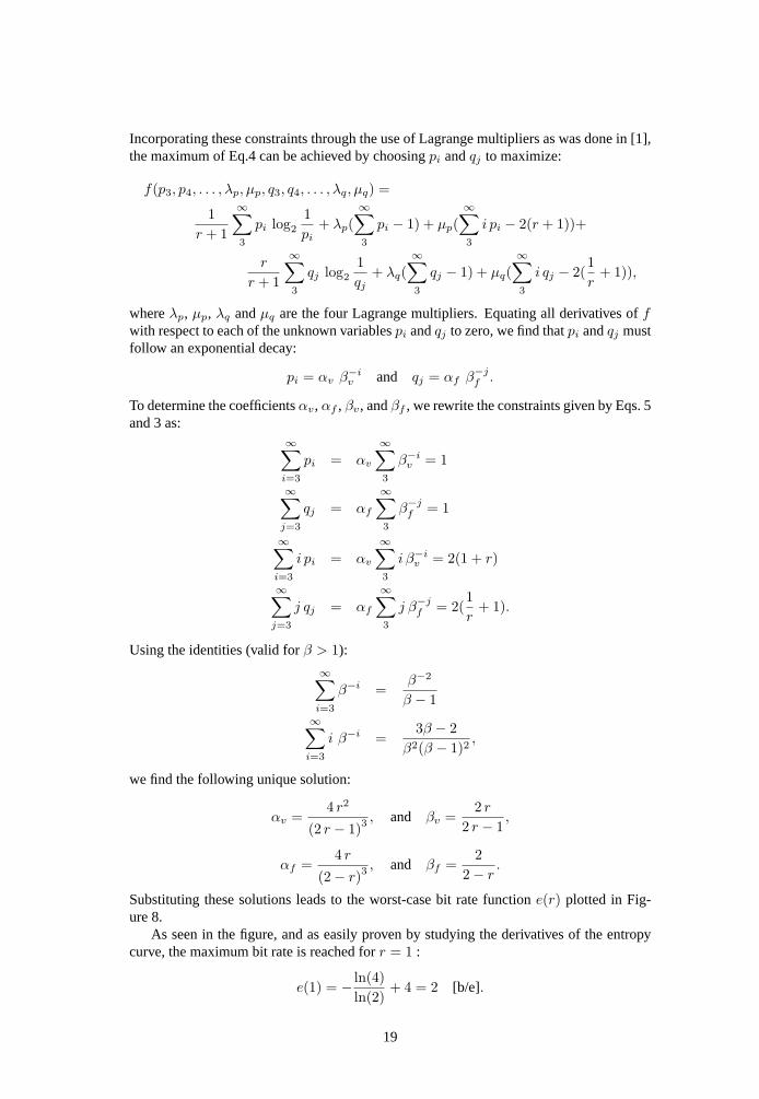
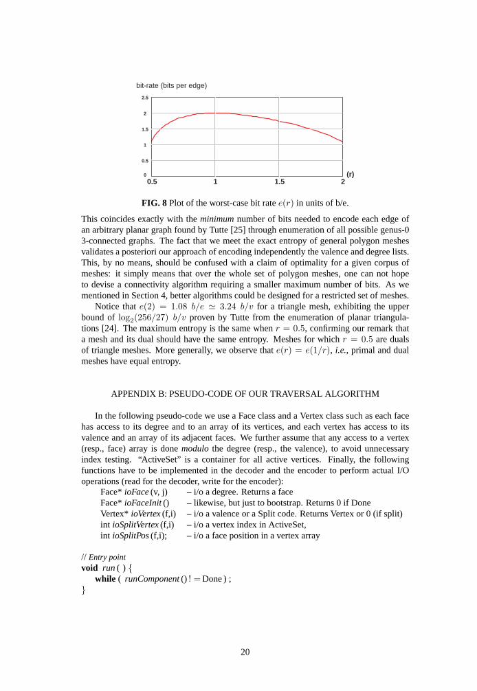
Substituting these solutions leads to the worst-case bit rate functione(r) plotted in Fig-ure8.
As seen in the figure, and as easily proven by studying the derivatives of the entropycurve, the maximum bit rate is reached forr = 1 :
e(1) = − ln(4)ln(2)
+ 4 = 2 [b/e].
19
0
0.5
1
1.5
2
2.5
0.5 1 1.5 2(r)
bit-rate (bits per edge)
FIG. 8 Plot of the worst-case bit ratee(r) in units of b/e.
This coincides exactly with theminimumnumber of bits needed to encode each edge ofan arbitrary planar graph found by Tutte [25] through enumeration of all possible genus-03-connected graphs. The fact that we meet the exact entropy of general polygon meshesvalidates a posteriori our approach of encoding independently the valence and degree lists.This, by no means, should be confused with a claim of optimality for a given corpus ofmeshes: it simply means that over the whole set of polygon meshes, one can not hopeto devise a connectivity algorithm requiring a smaller maximum number of bits. As wementioned in Section4, better algorithms could be designed for a restricted set of meshes.
Notice thate(2) = 1.08 b/e ' 3.24 b/v for a triangle mesh, exhibiting the upperbound oflog2(256/27) b/v proven by Tutte from the enumeration of planar triangula-tions [24]. The maximum entropy is the same whenr = 0.5, confirming our remark thata mesh and its dual should have the same entropy. Meshes for whichr = 0.5 are dualsof triangle meshes. More generally, we observe thate(r) = e(1/r), i.e., primal and dualmeshes have equal entropy.
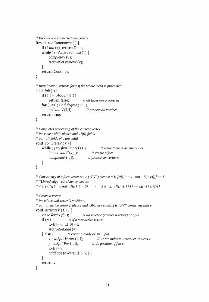
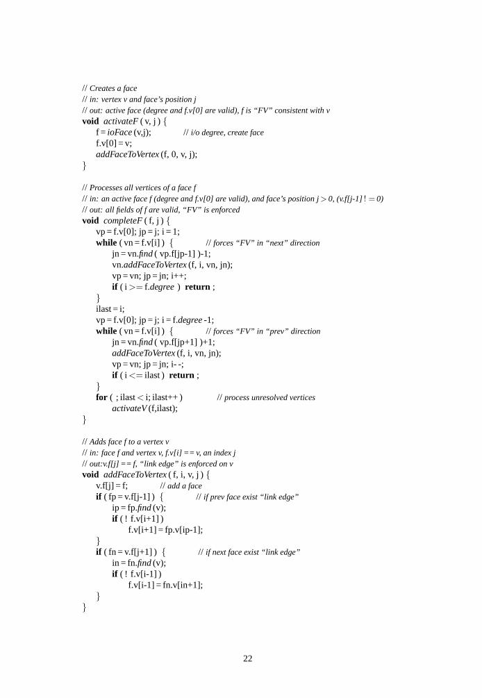
APPENDIX B: PSEUDO-CODE OF OUR TRAVERSAL ALGORITHM
In the following pseudo-code we use a Face class and a Vertex class such as each facehas access to its degree and to an array of its vertices, and each vertex has access to itsvalence and an array of its adjacent faces. We further assume that any access to a vertex(resp., face) array is donemodulothe degree (resp., the valence), to avoid unnecessaryindex testing. “ActiveSet” is a container for all active vertices. Finally, the followingfunctions have to be implemented in the decoder and the encoder to perform actual I/Ooperations (read for the decoder, write for the encoder):
Face*ioFace(v, j) – i/o a degree. Returns a faceFace*ioFaceInit() – likewise, but just to bootstrap. Returns 0 if DoneVertex* ioVertex(f,i) – i/o a valence or a Split code. Returns Vertex or 0 (if split)int ioSplitVertex(f,i) – i/o a vertex index in ActiveSet,int ioSplitPos(f,i); – i/o a face position in a vertex array
// Entry pointvoid run ( ) {
while ( runComponent() ! = Done ) ;}
20
// Process one connected componentResult runComponent( ) {
if ( ! init () ) return Done;while ( v=ActiveSet.next() ) {
completeV(v);ActiveSet.remove(v);
}return Continue;
}
// Initialization, returns false if the whole mesh is processedbool init ( ) {
if ( ! f = ioFaceInit() )return false; //all faces are processed
for ( i = 0 ; i < f.degree; i++ )activateV(f, i); // process all vertices
return true;}
// Completes processing of the current vertex.// in: v has valid valence and v.f[0] fields// out: all fields of v are validvoid completeV( v ) {
while ( j = v.firstEmpty() ) { // while there is an empty slotf = activateF(v, j); // create a facecompleteF(f, j); // process its vertices
}}
// Consistency of a face-vertex state (“FV”) means:∀ i: f.v[i] == v =⇒ ∃ j: v.f[j] == f// “Linked edge” consistency means:// ∀ j: (v.f[j] ! = 0 && v.f[j-1] ! = 0) =⇒ ∃ i1, i2: v.f[j].v[i1+1] == v.f[j-1].v[i2-1]
// Create a vertex// in: a face and vertex’s position i// out: an active vertex (valence and v.f[0] are valid), f is “FV” consistent with vvoid activateV( f, i ) {
v = ioVertex(f, i); // i/o valence (creates a vertex) or Splitif ( v ) { // if a new active vertex
f.v[i] = v; v.f[0] = f;ActiveSet.add(v);
} else{ // vertex already exists: Splitv = ioSplitVertex(f, i); // i/o v’s index in ActiveSet, returns vj = ioSplitPos(f, i); // i/o position of f in vf.v[i] = v;addFaceToVertex(f, i, v, j);
}return v;
}
21
// Creates a face// in: vertex v and face’s position j// out: active face (degree and f.v[0] are valid), f is “FV” consistent with vvoid activateF( v, j ) {
f = ioFace(v,j); // i/o degree, create facef.v[0] = v;addFaceToVertex(f, 0, v, j);
}
// Processes all vertices of a face f// in: an active face f (degree and f.v[0] are valid), and face’s position j> 0, (v.f[j-1] ! = 0)// out: all fields of f are valid, “FV” is enforcedvoid completeF( f, j ) {
vp = f.v[0]; jp = j; i = 1;while ( vn = f.v[i] ) { // forces “FV” in “next” direction
jn = vn.find( vp.f[jp-1] )-1;vn.addFaceToVertex(f, i, vn, jn);vp = vn; jp = jn; i++;if ( i >= f.degree) return ;
}ilast = i;vp = f.v[0]; jp = j; i = f.degree-1;while ( vn = f.v[i] ) { // forces “FV” in “prev” direction
jn = vn.find( vp.f[jp+1] )+1;addFaceToVertex(f, i, vn, jn);vp = vn; jp = jn; i- -;if ( i <= ilast ) return ;
}for ( ; ilast< i; ilast++ ) // process unresolved vertices
activateV(f,ilast);}
// Adds face f to a vertex v// in: face f and vertex v, f.v[i] == v, an index j// out:v.f[j] == f, “link edge” is enforced on vvoid addFaceToVertex( f, i, v, j ) {
v.f[j] = f; // add a faceif ( fp = v.f[j-1] ) { // if prev face exist “link edge”
ip = fp.find(v);if ( ! f.v[i+1] )
f.v[i+1] = fp.v[ip-1];}if ( fn = v.f[j+1] ) { // if next face exist “link edge”
in = fn.find(v);if ( ! f.v[i-1] )
f.v[i-1] = fn.v[in+1];}
}
22