Ann. Geophys., 30, 1379–1391, 2012www.ann-geophys.net/30/1379/2012/doi:10.5194/angeo-30-1379-2012© Author(s) 2012. CC Attribution 3.0 License.

AnnalesGeophysicae

Near real-time estimation of water vapour in the troposphere usingground GNSS and the meteorological data

J. Bosy, J. Kaplon, W. Rohm, J. Sierny, and T. Hadas

Institute of Geodesy and Geoinformatics, Wroclaw University of Environmental and Life Sciences, Grunwaldzka 53,50-357 Wroclaw, Poland

Correspondence to:J. Bosy (jaroslaw.bosy@up.wroc.pl)

Received: 4 April 2012 – Revised: 23 August 2012 – Accepted: 3 September 2012 – Published: 27 September 2012

Abstract. The near real-time (NRT) high resolution wa-ter vapour distribution models can be constructed based onGNSS observations delivered from Ground Base Augmenta-tion Systems (GBAS) and ground meteorological data. Since2008 in the territory of Poland, a GBAS system called ASG-EUPOS (Active Geodetic Network) has been operating. Thispaper addresses the problems concerning construction of theNRT model of water vapour distribution in the tropospherenear Poland. The first section presents all available GNSSand ground meteorological stations in the area of Poland andneighbouring countries. In this section, data feeding schemeis discussed, together with timeline and time resolution. Thehigh consistency between measured and interpolated tem-perature value is shown, whereas some discrepancy in thepressure is observed. In the second section, the NRT GNSSdata processing strategy of ASG-EUPOS network is dis-cussed. Preliminary results show fine alignment of the ob-tained Zenith Troposphere Delays (ZTDs) with referencedata from European Permanent Network (EPN) processingcenter. The validation of NRT troposphere products againstdaily solution shows 15 mm standard deviation of obtainedZTD differences. The last section presents the first resultsof 2-D water vapour distribution above the GNSS networkand application of the tomographic model to 3-D distributionof water vapour in the atmosphere. The GNSS tomographymodel, working on the simulated data from numerical fore-cast model, shows high consistency with the reference data(by means of standard deviation 4 mm km−1 or 4 ppm), how-ever, noise analysis shows high solution sensitivity to errorsin observations. The discrepancy for real data preliminary so-lution (measured as a mean standard deviation) between ref-erence NWP data and tomography data was on the level of9 mm km−1 (or 9 ppm) in terms of wet refractivity.

Keywords. Meteorology and atmospheric dynamics(Mesoscale meteorology; Synoptic-scale meteorology) –Radio science (Remote sensing)

1 Introduction

Global Navigation Satellite System (GNSS) was originallydesigned for positioning and navigation. Amongst other pos-sible applications it can also be used to derive informationabout the state of the atmosphere, what is now recognised asGNSS meteorology. Particularly GNSS meteorology is theremote-sensing of the atmosphere from a satellite platform(GNSS radio occultation meteorology) (Anthes et al., 2008;Wickert et al., 2009) and ground permanent stations (groundbased GNSS meteorology) (Bevis et al., 1992, 1994; Benderet al., 2011).

Continuous observations from GNSS receivers provide anexcellent tool for monitoring water vapour content in theEarth’s atmosphere. Several research projects were initiatedin Europe and overseas to derive the water vapour con-tent in the atmosphere from ground-based GNSS observationdata, for example: COST Action 716 (European Cooperationin the field of Scientific Technical Research-exploitation ofground-based GPS for climate and numerical weather predic-tion applications, 1998–2004) (van der Marel, 2004; Dousa,2004), TOUGH (Targeting Optimal Use of GPS HumidityData in Meteorology, 2003–2006) (Vedel and Huang, 2004;Jarvinen et al., 2007) and E-GVAP (The EUMETNET GPSWater Vapour Programme, 2004–) (Dousa, 2010a; Bennittand Jupp, 2012). The near real-time (NRT) GNSS watervapour monitoring for numerical weather prediction services

Published by Copernicus Publications on behalf of the European Geosciences Union.

1380 J. Bosy et al.: Near real-time estimation of water vapour in troposphere

are active in Germany (Heise et al., 2009) and Austria (Kara-batic et al., 2011).

The GNSS meteorology is based on the results of GNSSdata processing represented by the Zenith Total Delay (ZTD).The ZTD can be split into hydrostatic ZHD and wet ZWDcomponent of the delay:

ZTD= ZHD+ZWD (1)

The hydrostatic component ZHD is modelled based on thepressure or pressure and temperature at the GNSS stationswhich might be obtained from deterministic atmospheremodels, as well as Numerical Weather Prediction (NWP)models or from ground meteorological observations.

The wet component of Zenith Tropospheric Delay (ZWD)is the foundation for the computing of water vapour contentin the atmosphere. The integrated content of water vapourabove GNSS stations (2-D model), represented by IntegratedWater Vapour (IWV), is obtained directly from ZWD apply-ing empirical equations (Bevis et al., 1992, 1994).

The spatial structure and temporal behaviour of the watervapour in the troposphere (3-D) can be modelled using theGNSS tomography method. In principle, GNSS tomographyis founded on the linear equation relating Slant Wet Delay(SWD) with the wet refractivity in voxelsNw along the ray-path which reads as follows (i.e.,Flores et al., 2000):

SWD= A ·Nw (2)

whereA is the design matrix.Wet refractivityNw is a dimensionless quantity and by def-

inition of refraction contains 10−6 term, therefore, may bepresented either in ppm or in mm km−1 (interchangeable). Inthis study, authors choose to present wet refractivity resultsin mm km−1.

The design matrix construction is at the focal point of alltomography applications (Perler et al., 2011; Nilsson andGradinarsky, 2006), because it relates to the SWD sum ofall wet refractivities voxels along the path multiplied by thedistance that the signal resides in each voxel, which is a lin-ear operator. Currently several methods exist to solve Eq. (2).The first is to add horizontal and vertical constraints into thesystem of equations (2) and then solve it (Hirahara, 2000),the second is to use a Kalman filter with the same equa-tion system (Flores et al., 2000), the third is to find the so-lution directly from the GNSS phase measurement equation(Nilsson and Gradinarsky, 2006) and another is AlgebraicReconstruction Technique (ART) (Bender et al., 2011). Inprevious papers byRohm and Bosy(2009, 2011), the au-thors showed GNSS tomography methodology studies basedon minimum constraint solution and Singular Value Decom-position (SVD) algorithm (Anderson et al., 1999) to find thewet refractivity (Eq.2) above the network of GNSS receivers.

A number of GNSS applications require precise position-ing with high accuracy in real-time or rapid static postpro-cessing mode. Precise positioning in real-time or rapid static

Stations:EPNNationalForeign

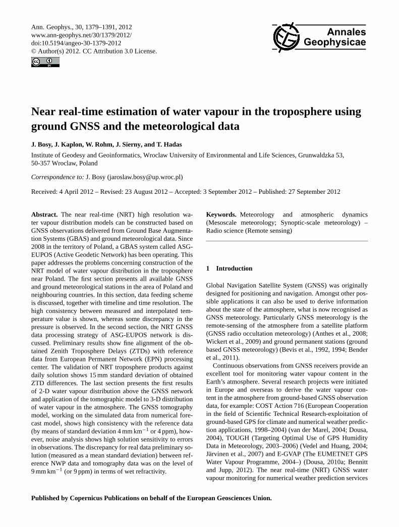
Fig. 1. Reference stations of ASG-EUPOS system(www.asgeupos.pl): 15 EPN, 85 national, 25 foreign (7 Novem-ber 2011).

mode is currently being implemented in two methods: dif-ferential and autonomous. The positioning using the abovemethods can be supported by Ground Base AugmentationSystem (GBAS), which provides better results stability inthe area of the GBAS network (Kee et al., 1991). One ofthe elements supporting precise positioning, especially forheight component, is a model of the neutral atmosphere (tro-posphere), computed for the GBAS network area (Wielgoszet al., 2011; Grejner-Brzezinska et al., 2009). The Poland ter-ritory is covered by dense network of GNSS stations in theframe of a GBAS system called ASG-EUPOS.

The first part of the paper contains the procedure of inte-gration and validation of ground-based meteorological obser-vations delivered from various sources on the area of GBASASG-EUPOS network. The second part presents the method-ology of NRT GNSS data processing of ASG-EUPOS sta-tions for ZTD estimation with reference data and productsfrom EPN/IGS processing centers. The third part presentsthe procedure of water vapour 2-D distribution above GNSSstations and tomographic model application to estimate 3-Ddistribution of water vapour in the atmosphere.

2 GNSS and meteorological data

The ASG-EUPOS system permanently collects the GNSSdata from 125 stations (Fig.1).

Complying with the EUPOS organisation (www.eupos.org) and the project of the ASG-EUPOS system stan-dards, the distances between neighbouring reference sta-tions should be 70 km which gives the number of stations100 in the area of Poland. According to the rules of theEUPOS organisation (in the frame of cross-border data

Ann. Geophys., 30, 1379–1391, 2012 www.ann-geophys.net/30/1379/2012/

J. Bosy et al.: Near real-time estimation of water vapour in troposphere 1381

REDZ

LAMASWKI

GWWL

BYDG

BOGI

BPDLJOZ2

LODZ

BOR1

WROC

KATO

KRA1

ZYWI

USDL

Stations:

ASG-EUPOS

METAR

SYNOP

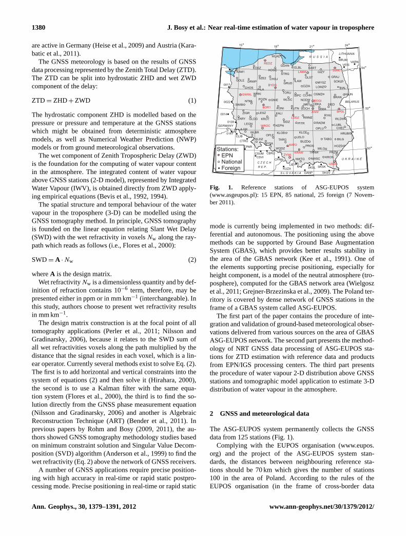
Fig. 2. Ground stations of meteorological networks (ASG-EUPOS:15, METAR: 22, SYNOP: 84) in the area of Poland (7 Novem-ber 2011).

exchange) the reference stations from Lithuania (LITPOS),Germany (SAPOS), Czech Republic (CZEPOS) and Slo-vakia (SKPOS) were added to the regular processing of theASG-EUPOS network (Fig.1) (Bosy et al., 2008).

In all localisations of the EUREF Permanent Network(EPN) stations (Fig.1) in 2008, the new uniform meteorolog-ical infrastructure was installed. In all stations the basic me-teorological parameters (pressure with precision±0.08 hPafrom 500 to 1100 hPa, temperature with precision±0.2◦Cfrom −50 to+60◦C and relative humidity with precision±2 % from 0 to 100 %) are measured close to the GNSS an-tenna. This set of meteorological sensors are considered themost unified, homogenous (available with 1 h time resolu-tion) and most consistent, therefore, in this study they areregarded as reference.

The ground meteorological observations in the areaof Poland and neighbouring countries are also availablefrom meteorological stations acting as a support for avi-ation: METAR (Meteorological Terminal Aviation RoutineWeather Report or Meteorological Aerodrome Report) mes-sages stations, or as a country meteorological data supply:SYNOP (surface synoptic observations) messages stations(Fig. 2).

The data are available with different time resolution(SYNOP: 3 h, METAR: 0.5 h). While the spatial distributionof METAR, SYNOP stations is complying with near real-time estimation of water vapour needs, the actual quality ofthe data remains unknown. This set of sensors is more densethan the previously mentioned and could be used to interpo-late meteorological parameters for the rest of ASG-EUPOSGNSS stations not equipped with meteorological instrumen-tation.

S [x,y,h,T,P,H]i i

wi

wi

wi

wi

S [x,y,h,T,P,H]i i

S [x,y,h,T,P,H]i i

S [x,y,h,T,P,H]i i

[x,y,h](T,P,H) ?

i

i

Pi

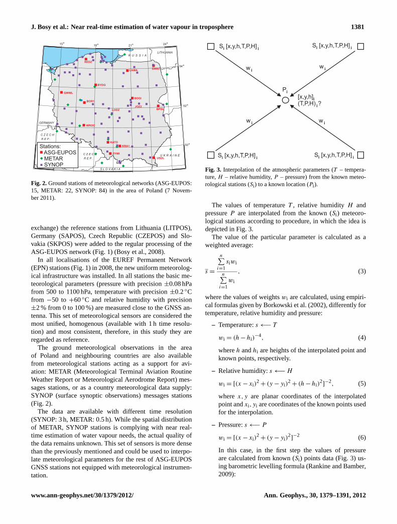
Fig. 3. Interpolation of the atmospheric parameters (T – tempera-ture,H – relative humidity,P – pressure) from the known meteo-rological stations (Si ) to a known location (Pi ).

The values of temperatureT , relative humidityH andpressureP are interpolated from the known (Si) meteoro-logical stations according to procedure, in which the idea isdepicted in Fig.3.

The value of the particular parameter is calculated as aweighted average:

s =

n∑i=1

siwi

n∑i=1

wi

, (3)

where the values of weightswi are calculated, using empiri-cal formulas given byBorkowski et al.(2002), differently fortemperature, relative humidity and pressure:

– Temperature:s←− T

wi = (h−hi)−4, (4)

whereh andhi are heights of the interpolated point andknown points, respectively.

– Relative humidity:s←−H

wi = [(x− xi)2+ (y− yi)

2+ (h−hi)

2]−2, (5)

where x,y are planar coordinates of the interpolatedpoint andxi,yi are coordinates of the known points usedfor the interpolation.

– Pressure:s←− P

wi = [(x− xi)2+ (y− yi)

2]−2 (6)

In this case, in the first step the values of pressureare calculated from known (Si) points data (Fig.3) us-ing barometric levelling formula (Rankine and Bamber,2009):

www.ann-geophys.net/30/1379/2012/ Ann. Geophys., 30, 1379–1391, 2012

1382 J. Bosy et al.: Near real-time estimation of water vapour in troposphere

0

5

10

15

BP

DL

Temperature [deg. C]

60

80

100

Relative humidity [%]

1004

1006

1008

1010

Pressure [mbar]

0

5

10

15B

YD

G

60

80

100

1005

1010

1015

1020

0 6 12 18 24−10

0

10

20

Hourly sessions

ZY

WI

0 6 12 18 240

50

100

Hourly sessions

0 6 12 18 24975

980

985

990

Hourly sessions

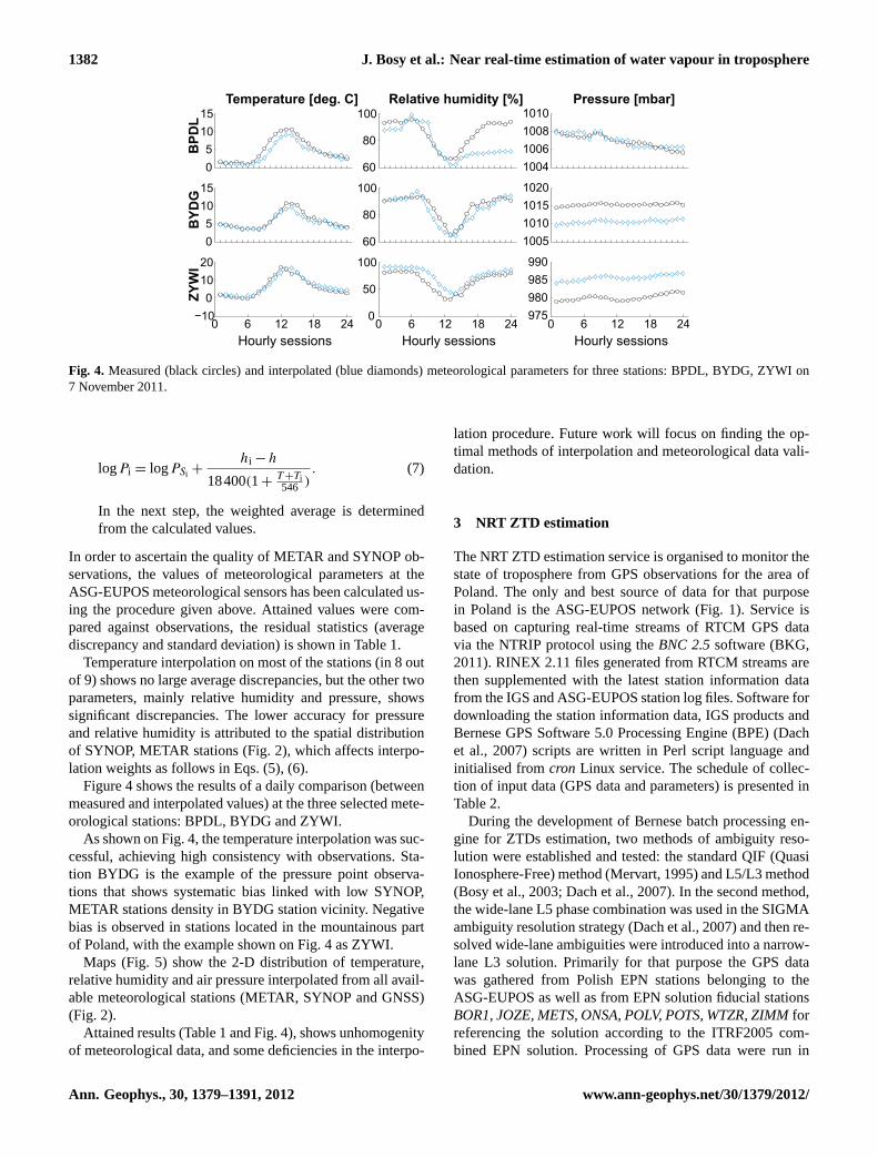
Fig. 4. Measured (black circles) and interpolated (blue diamonds) meteorological parameters for three stations: BPDL, BYDG, ZYWI on7 November 2011.

logPi = logPSi +hi −h

18400(1+ T+Ti546 )

. (7)

In the next step, the weighted average is determinedfrom the calculated values.

In order to ascertain the quality of METAR and SYNOP ob-servations, the values of meteorological parameters at theASG-EUPOS meteorological sensors has been calculated us-ing the procedure given above. Attained values were com-pared against observations, the residual statistics (averagediscrepancy and standard deviation) is shown in Table1.

Temperature interpolation on most of the stations (in 8 outof 9) shows no large average discrepancies, but the other twoparameters, mainly relative humidity and pressure, showssignificant discrepancies. The lower accuracy for pressureand relative humidity is attributed to the spatial distributionof SYNOP, METAR stations (Fig.2), which affects interpo-lation weights as follows in Eqs. (5), (6).

Figure4 shows the results of a daily comparison (betweenmeasured and interpolated values) at the three selected mete-orological stations: BPDL, BYDG and ZYWI.

As shown on Fig.4, the temperature interpolation was suc-cessful, achieving high consistency with observations. Sta-tion BYDG is the example of the pressure point observa-tions that shows systematic bias linked with low SYNOP,METAR stations density in BYDG station vicinity. Negativebias is observed in stations located in the mountainous partof Poland, with the example shown on Fig.4 as ZYWI.

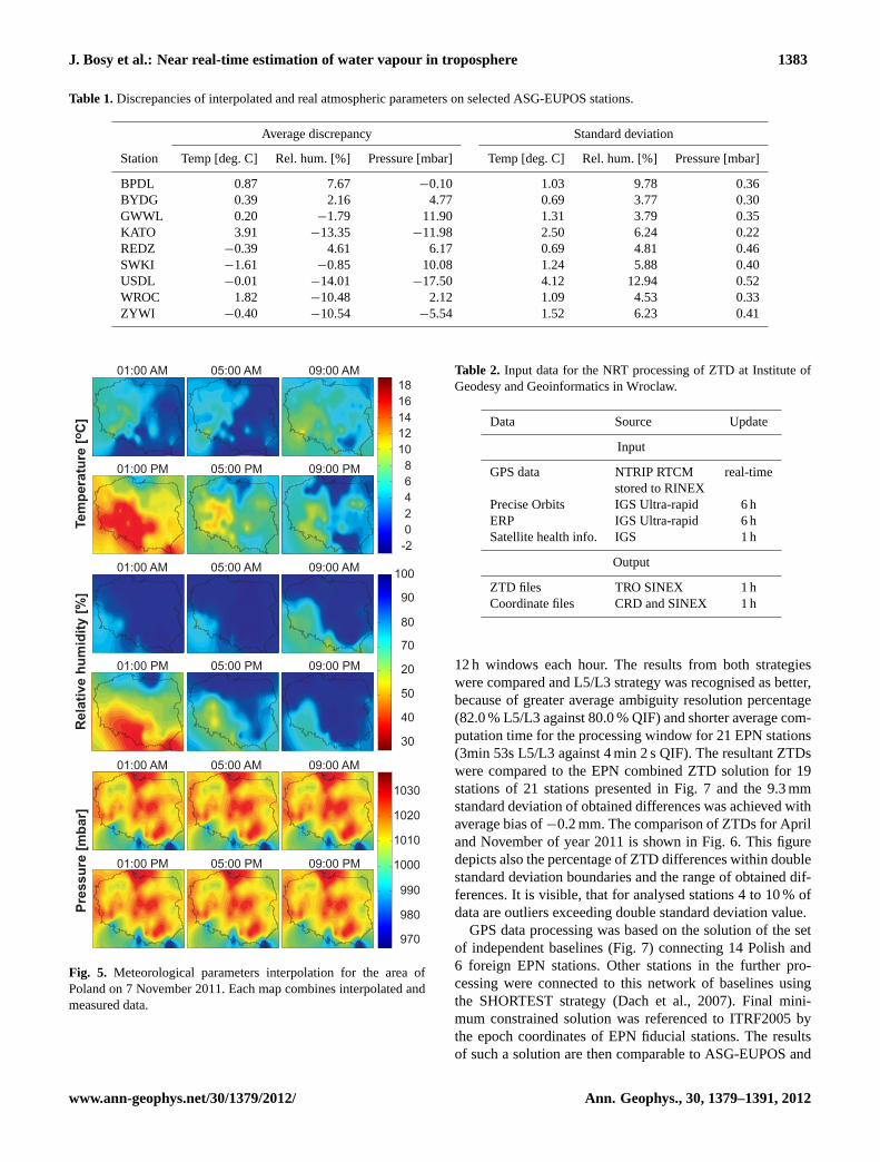
Maps (Fig.5) show the 2-D distribution of temperature,relative humidity and air pressure interpolated from all avail-able meteorological stations (METAR, SYNOP and GNSS)(Fig. 2).

Attained results (Table1 and Fig.4), shows unhomogenityof meteorological data, and some deficiencies in the interpo-

lation procedure. Future work will focus on finding the op-timal methods of interpolation and meteorological data vali-dation.

3 NRT ZTD estimation

The NRT ZTD estimation service is organised to monitor thestate of troposphere from GPS observations for the area ofPoland. The only and best source of data for that purposein Poland is the ASG-EUPOS network (Fig.1). Service isbased on capturing real-time streams of RTCM GPS datavia the NTRIP protocol using theBNC 2.5software (BKG,2011). RINEX 2.11 files generated from RTCM streams arethen supplemented with the latest station information datafrom the IGS and ASG-EUPOS station log files. Software fordownloading the station information data, IGS products andBernese GPS Software 5.0 Processing Engine (BPE) (Dachet al., 2007) scripts are written in Perl script language andinitialised fromcron Linux service. The schedule of collec-tion of input data (GPS data and parameters) is presented inTable2.

During the development of Bernese batch processing en-gine for ZTDs estimation, two methods of ambiguity reso-lution were established and tested: the standard QIF (QuasiIonosphere-Free) method (Mervart, 1995) and L5/L3 method(Bosy et al., 2003; Dach et al., 2007). In the second method,the wide-lane L5 phase combination was used in the SIGMAambiguity resolution strategy (Dach et al., 2007) and then re-solved wide-lane ambiguities were introduced into a narrow-lane L3 solution. Primarily for that purpose the GPS datawas gathered from Polish EPN stations belonging to theASG-EUPOS as well as from EPN solution fiducial stationsBOR1, JOZE, METS, ONSA, POLV, POTS, WTZR, ZIMMforreferencing the solution according to the ITRF2005 com-bined EPN solution. Processing of GPS data were run in

Ann. Geophys., 30, 1379–1391, 2012 www.ann-geophys.net/30/1379/2012/

J. Bosy et al.: Near real-time estimation of water vapour in troposphere 1383

Table 1.Discrepancies of interpolated and real atmospheric parameters on selected ASG-EUPOS stations.

Average discrepancy Standard deviation

Station Temp [deg. C] Rel. hum. [%] Pressure [mbar] Temp [deg. C] Rel. hum. [%] Pressure [mbar]

BPDL 0.87 7.67 −0.10 1.03 9.78 0.36BYDG 0.39 2.16 4.77 0.69 3.77 0.30GWWL 0.20 −1.79 11.90 1.31 3.79 0.35KATO 3.91 −13.35 −11.98 2.50 6.24 0.22REDZ −0.39 4.61 6.17 0.69 4.81 0.46SWKI −1.61 −0.85 10.08 1.24 5.88 0.40USDL −0.01 −14.01 −17.50 4.12 12.94 0.52WROC 1.82 −10.48 2.12 1.09 4.53 0.33ZYWI −0.40 −10.54 −5.54 1.52 6.23 0.41

01:00 AM 05:00 AM 09:00 AM

01:00 PM 05:00 PM 09:00 PM

01:00 AM 05:00 AM 09:00 AM

01:00 PM 05:00 PM 09:00 PM

01:00 AM 05:00 AM 09:00 AM

01:00 PM 05:00 PM 09:00 PM

Te

mp

era

ture

[C

]o

Re

lati

ve

hu

mid

ity

[%

]P

res

su

re [

mb

ar]

18

16

14

12

10

8

6

4

2

0

-2

100

90

80

70

20

50

40

30

1030

1020

1010

1000

990

980

970

Fig. 5. Meteorological parameters interpolation for the area ofPoland on 7 November 2011. Each map combines interpolated andmeasured data.

Table 2. Input data for the NRT processing of ZTD at Institute ofGeodesy and Geoinformatics in Wroclaw.

Data Source Update

Input

GPS data NTRIP RTCM real-timestored to RINEX

Precise Orbits IGS Ultra-rapid 6 hERP IGS Ultra-rapid 6 hSatellite health info. IGS 1 h

Output

ZTD files TRO SINEX 1 hCoordinate files CRD and SINEX 1 h

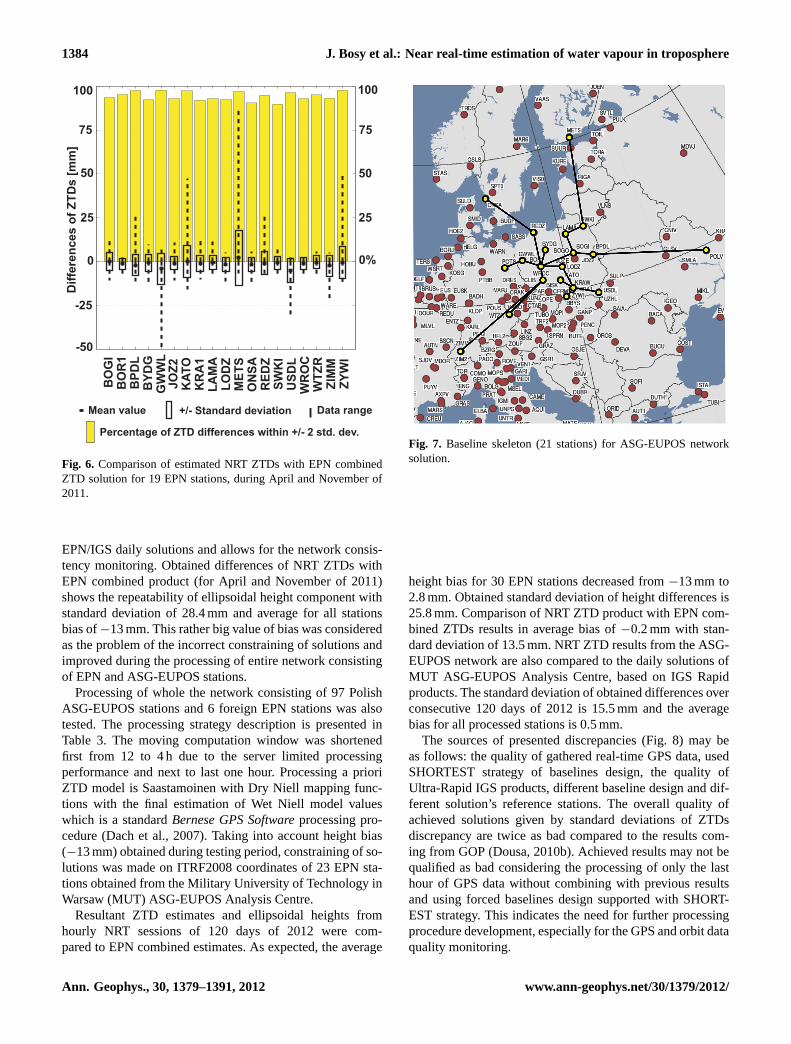
12 h windows each hour. The results from both strategieswere compared and L5/L3 strategy was recognised as better,because of greater average ambiguity resolution percentage(82.0 % L5/L3 against 80.0 % QIF) and shorter average com-putation time for the processing window for 21 EPN stations(3min 53s L5/L3 against 4 min 2 s QIF). The resultant ZTDswere compared to the EPN combined ZTD solution for 19stations of 21 stations presented in Fig.7 and the 9.3 mmstandard deviation of obtained differences was achieved withaverage bias of−0.2 mm. The comparison of ZTDs for Apriland November of year 2011 is shown in Fig.6. This figuredepicts also the percentage of ZTD differences within doublestandard deviation boundaries and the range of obtained dif-ferences. It is visible, that for analysed stations 4 to 10 % ofdata are outliers exceeding double standard deviation value.

GPS data processing was based on the solution of the setof independent baselines (Fig.7) connecting 14 Polish and6 foreign EPN stations. Other stations in the further pro-cessing were connected to this network of baselines usingthe SHORTEST strategy (Dach et al., 2007). Final mini-mum constrained solution was referenced to ITRF2005 bythe epoch coordinates of EPN fiducial stations. The resultsof such a solution are then comparable to ASG-EUPOS and

www.ann-geophys.net/30/1379/2012/ Ann. Geophys., 30, 1379–1391, 2012

1384 J. Bosy et al.: Near real-time estimation of water vapour in troposphere

Fig. 6. Comparison of estimated NRT ZTDs with EPN combinedZTD solution for 19 EPN stations, during April and November of2011.

EPN/IGS daily solutions and allows for the network consis-tency monitoring. Obtained differences of NRT ZTDs withEPN combined product (for April and November of 2011)shows the repeatability of ellipsoidal height component withstandard deviation of 28.4 mm and average for all stationsbias of−13 mm. This rather big value of bias was consideredas the problem of the incorrect constraining of solutions andimproved during the processing of entire network consistingof EPN and ASG-EUPOS stations.

Processing of whole the network consisting of 97 PolishASG-EUPOS stations and 6 foreign EPN stations was alsotested. The processing strategy description is presented inTable 3. The moving computation window was shortenedfirst from 12 to 4 h due to the server limited processingperformance and next to last one hour. Processing a prioriZTD model is Saastamoinen with Dry Niell mapping func-tions with the final estimation of Wet Niell model valueswhich is a standardBernese GPS Softwareprocessing pro-cedure (Dach et al., 2007). Taking into account height bias(−13 mm) obtained during testing period, constraining of so-lutions was made on ITRF2008 coordinates of 23 EPN sta-tions obtained from the Military University of Technology inWarsaw (MUT) ASG-EUPOS Analysis Centre.

Resultant ZTD estimates and ellipsoidal heights fromhourly NRT sessions of 120 days of 2012 were com-pared to EPN combined estimates. As expected, the average

Fig. 7. Baseline skeleton (21 stations) for ASG-EUPOS networksolution.

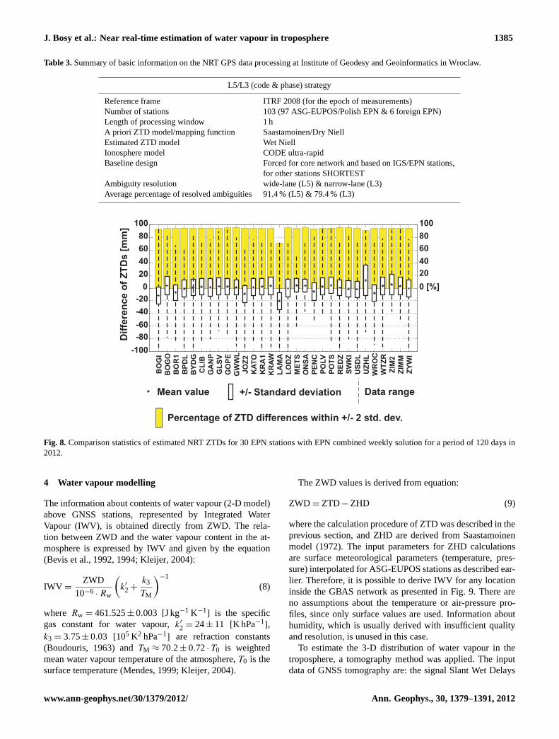
height bias for 30 EPN stations decreased from−13 mm to2.8 mm. Obtained standard deviation of height differences is25.8 mm. Comparison of NRT ZTD product with EPN com-bined ZTDs results in average bias of−0.2 mm with stan-dard deviation of 13.5 mm. NRT ZTD results from the ASG-EUPOS network are also compared to the daily solutions ofMUT ASG-EUPOS Analysis Centre, based on IGS Rapidproducts. The standard deviation of obtained differences overconsecutive 120 days of 2012 is 15.5 mm and the averagebias for all processed stations is 0.5 mm.

The sources of presented discrepancies (Fig.8) may beas follows: the quality of gathered real-time GPS data, usedSHORTEST strategy of baselines design, the quality ofUltra-Rapid IGS products, different baseline design and dif-ferent solution’s reference stations. The overall quality ofachieved solutions given by standard deviations of ZTDsdiscrepancy are twice as bad compared to the results com-ing from GOP (Dousa, 2010b). Achieved results may not bequalified as bad considering the processing of only the lasthour of GPS data without combining with previous resultsand using forced baselines design supported with SHORT-EST strategy. This indicates the need for further processingprocedure development, especially for the GPS and orbit dataquality monitoring.

Ann. Geophys., 30, 1379–1391, 2012 www.ann-geophys.net/30/1379/2012/

J. Bosy et al.: Near real-time estimation of water vapour in troposphere 1385

Table 3.Summary of basic information on the NRT GPS data processing at Institute of Geodesy and Geoinformatics in Wroclaw.

L5/L3 (code & phase) strategy

Reference frame ITRF 2008 (for the epoch of measurements)Number of stations 103 (97 ASG-EUPOS/Polish EPN & 6 foreign EPN)Length of processing window 1 hA priori ZTD model/mapping function Saastamoinen/Dry NiellEstimated ZTD model Wet NiellIonosphere model CODE ultra-rapidBaseline design Forced for core network and based on IGS/EPN stations,

for other stations SHORTESTAmbiguity resolution wide-lane (L5) & narrow-lane (L3)Average percentage of resolved ambiguities 91.4 % (L5) & 79.4 % (L3)

Fig. 8. Comparison statistics of estimated NRT ZTDs for 30 EPN stations with EPN combined weekly solution for a period of 120 days in2012.

4 Water vapour modelling

The information about contents of water vapour (2-D model)above GNSS stations, represented by Integrated WaterVapour (IWV), is obtained directly from ZWD. The rela-tion between ZWD and the water vapour content in the at-mosphere is expressed by IWV and given by the equation(Bevis et al., 1992, 1994; Kleijer, 2004):

IWV =ZWD

10−6 ·Rw

(k′2+

k3

TM

)−1

(8)

where Rw = 461.525±0.003 [J kg−1 K−1] is the specific

gas constant for water vapour,k′2= 24±11 [K hPa−1],

k3= 3.75±0.03 [105 K2 hPa−1] are refraction constants

(Boudouris, 1963) and TM ≈ 70.2±0.72· T0 is weightedmean water vapour temperature of the atmosphere,T0 is thesurface temperature (Mendes, 1999; Kleijer, 2004).

The ZWD values is derived from equation:

ZWD= ZTD−ZHD (9)

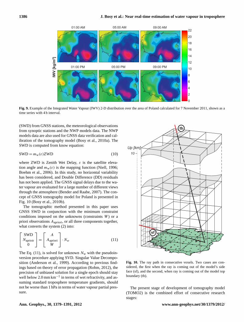
where the calculation procedure of ZTD was described in theprevious section, and ZHD are derived from Saastamoinenmodel (1972). The input parameters for ZHD calculationsare surface meteorological parameters (temperature, pres-sure) interpolated for ASG-EUPOS stations as described ear-lier. Therefore, it is possible to derive IWV for any locationinside the GBAS network as presented in Fig.9. There areno assumptions about the temperature or air-pressure pro-files, since only surface values are used. Information abouthumidity, which is usually derived with insufficient qualityand resolution, is unused in this case.

To estimate the 3-D distribution of water vapour in thetroposphere, a tomography method was applied. The inputdata of GNSS tomography are: the signal Slant Wet Delays

www.ann-geophys.net/30/1379/2012/ Ann. Geophys., 30, 1379–1391, 2012

1386 J. Bosy et al.: Near real-time estimation of water vapour in troposphere

IWV

[kg

/m]

2

Fig. 9.Example of the Integrated Water Vapour (IWV) 2-D distribution over the area of Poland calculated for 7 November 2011, shown as atime series with 4 h interval.

(SWD) from GNSS stations, the meteorological observationsfrom synoptic stations and the NWP models data. The NWPmodels data are also used for GNSS data verification and cal-ibration of the tomography model (Bosy et al., 2010a). TheSWD is computed from know equation:

SWD=mw(ε)ZWD (10)

where ZWD is Zenith Wet Delay,ε is the satellite eleva-tion angle andmw(ε) is the mapping function (Niell, 1996;Boehm et al., 2006). In this study, no horizontal variabilityhas been considered, and Double Difference (DD) residualshas not been applied. The GNSS signal delays due to the wa-ter vapour are evaluated for a large number of different viewsthrough the atmosphere (Bender and Raabe, 2007). The con-cept of GNSS tomography model for Poland is presented inFig. 10 (Bosy et al., 2010b).

The tomographic method presented in this paper usesGNSS SWD in conjunction with the minimum constraintconditions imposed on the unknowns (constraintsW ) or apriori observationsAapriori, or all three components together,what converts the system (2) into: SWD

Naprioir0

= A

AaprioriW

·Nw (11)

The Eq. (11), is solved for unknownNw with the pseudoin-version procedure applying SVD. Singular Value Decompo-sition (Anderson et al., 1999). According to previous find-ings based on theory of error propagation (Rohm, 2012), theprecision of unbiased solution for a single epoch should staywell below 2.0 mm km−1 in terms of wet refractivity, and as-suming standard troposphere temperature gradients, shouldnot be worse than 1 hPa in terms of water vapour partial pres-sure.

sf

tb

10

Up [km]

Fig. 10. The ray path in consecutive voxels. Two cases are con-sidered, the first when the ray is coming out of the model’s sideface (sf), and the second, when ray is coming out of the model topboundary (tb).

The present stage of development of tomography model(TOMO2) is the combined effort of consecutive researchstages:

Ann. Geophys., 30, 1379–1391, 2012 www.ann-geophys.net/30/1379/2012/

J. Bosy et al.: Near real-time estimation of water vapour in troposphere 1387

0 2 4 6 8 100

1

2

3

4

5

6

7

8x 10

5

Easting [m]

No

rth

ing

[m

]

faces intersections (inner)

voxel centroid (inner)

faces intersections (outer)

voxel centroid (outer)

x 105

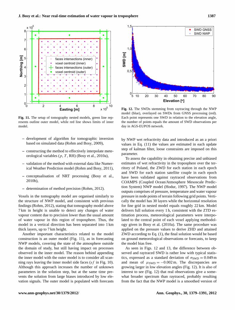
Fig. 11. The setup of tomography nested models, green line rep-resents outline outer model, while red line shows limits of innermodel.

– development of algorithm for tomographic inversionbased on simulated data (Rohm and Bosy, 2009),

– constructing the method to effectively interpolate mete-orological variables (p, T , RH) (Bosy et al., 2010a),

– validation of the method with external data like Numer-ical Weather Prediction model (Rohm and Bosy, 2011),

– conceptualisation of NRT processing (Bosy et al.,2010b),

– determination of method precision (Rohm, 2012).

Voxels in the tomography model are organised similarly tothe structure of NWP model, and consistent with previousfindings (Rohm, 2012), stating that tomography model above7 km in height is unable to detect any changes of watervapour content due to precision lower than the usual amountof water vapour in this region of troposphere. Thus, themodel in a vertical direction has been separated into 1 kmthick layers, up to 7 km height.

Another important characteristics related to the modelconstruction is an outer model (Fig.11), as in forecastingNWP models, covering the state of the atmosphere outsidethe domain of study, but still having impact on processesobserved in the inner model. The reason behind appendingthe inner model with the outer model is to consider all scan-ning rays leaving the inner model side faces (sf in Fig. 10).Although this approach increases the number of unknownparameters in the solution step, but at the same time pre-vents the solution from large biases introduced by low ele-vation signals. The outer model is populated with forecasts

5 10 20 30 40 50 60 70 80 900

0,5

1,0

1,5

Elevation [ ]o

SW

D [

m]

SWD GNSS

SWD NWP

Fig. 12. The SWDs stemming from raytracing through the NWPmodel (blue), overlayed on SWDs from GNSS processing (red).Each point represents one SWD in relation to the elevation angle,the number of points equals the amount of SWD observations perday in AGS-EUPOS network.

by NWP wet refractivity data and introduced as an a priorivalues in Eq. (11) the values are estimated in each updatestep of kalman filter, loose constraints are imposed on thisparameter.

To assess the capability in obtaining precise and unbiasedestimates of wet refractivity in the troposphere over the ter-ritory of Poland, the ZWD for each station in each epochand SWD for each station satellite couple in each epochhave been validated against raytraced observations fromCOAMPS (Coupled Ocean/Atmosphere Mesoscale Predic-tion System) NWP model (Hodur, 1997). The NWP modeloutputs comprises of pressure, temperature and water vapourpressure in node points of terrain following grid points. Verti-cally the model has 30 layers while the horizontal resolutionfor fine grid in nested model equals roughly 22 km. Modeldelivers full solution every 1 h, consistent with the ZTD es-timation process, meteorological parameters were interpo-lated to the central point of each voxel applying methodol-ogy given inBosy et al.(2010a). The same procedure wasapplied on the pressure values to derive ZHD and attainedZWD according to Eq. (1), the final solution would be basedon ground meteorological observations or forecasts, to keepthe model bias free.

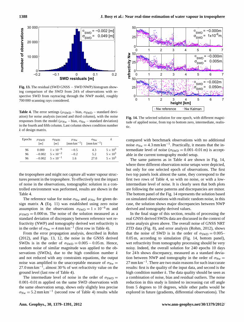
As seen in Figs.12 and 13, the difference between ob-served and raytraced SWD is rather low with typical statis-tics, expressed as a standard deviation ofσSWD= 0.049 mand mean ofµSWD=−0.002 m. The discrepancies aregrowing larger in low elevation angles (Fig.12). It is also ofinterest to see (Fig.12) that real observations give a some-what broader spectrum than raytraced, probably resultingfrom the fact that the NWP model is a smoothed version of

www.ann-geophys.net/30/1379/2012/ Ann. Geophys., 30, 1379–1391, 2012

1388 J. Bosy et al.: Near real-time estimation of water vapour in troposphere

−0.2 −0.1 0 0.1 0.20

10 000

20 000

30 000

SWD residuals [m]

nu

mb

er

of

ob

serv

ati

on

s αSWD

= −0.002 [m]

σSWD

= 0.049 [m]

Fig. 13.The residual (SWD GNSS− SWD NWP) histogram show-ing comparison of the SWD from 24 h of observations with re-spective SWD from raytracing through the NWP model, roughly700 000 scanning rays considered.

Table 4. The error settings (µSWD – bias,σSWD – standard devi-ation) for noise analysis (second and third column), with the noiseresponses from the model (µNw – bias,σNw – standard deviation)in the fourth and fifth column. Last column shows condition numberk of design matrix.

Epochs µSWD σSWD µNw σNw k

[m] [m] [mm km−1] [mm km−1

]

96 0.000 1×10−6−0.5 4.3 5×103

96 −0.002 5×10−2−0.2 5.2 5×103

96 −0.002 5×10−1 1.6 27.0 5×103

the troposphere and might not capture all water vapour struc-tures present in the troposphere. To effectively test the impactof noise in the observations, tomographic solution in a con-trolled environment was performed, results are shown in theTable4.

The reference value for noiseσNw andµNw for given de-sign matrix A (Eq. 11) was established using zero noiseassumption in the observationsσSWD= 1×10−6 m andµSWD= 0.000 m. The noise of the solution measured as astandard deviation of discrepancy between reference wet re-fractivity (NWP) and tomography derived wet refractivity isin the order ofσNw = 4 mm km−1 (first row in Table4).

From the error propagation analysis, described inRohm(2012), and Figs.13, 12, the noise in the GNSS derivedSWDs is in the order ofσSWD= 0.005−0.05 m. Hence,random noise of similar magnitude was applied to the ob-servations (SWDs), due to the high condition numberk

and not reduced with any constraints equations, the outputnoise was amplified to the unacceptable measure ofσNw =

27.0 mm km−1, almost 30 % of wet refractivity value on theground level (last row of Table4).

The intermediate level of noise in the order ofσSWD=

0.001–0.01 m applied on the same SWD observations withthe same observation setup, shows only slightly less preciseσNw = 5.2 mm km−1 (second row of Table4) results while

0 1 2 3 4 5 6 7

0

25

50

0 1 2 3 4 5 6 7

0

25

50

refr

ac

tiv

ity

Nw

0 1 2 3 4 5 6 7

0

25

50

height [km]

αSWD

= −0.000m

σSWD

= 1x10 m-6

αSWD

= −0.002m

σSWD

= 0.050m

αSWD

= −0.000m

σSWD

= 0.005m

Nw reference Nw Kalman

Fig. 14.The selected solution for one epoch, with different magni-tude of applied noise, from top to bottom zero, intermediate, realis-tic.

compared with benchmark observations with no additionalnoiseσNw = 4.3 mm km−1. Practically, it means that the in-termediate level of noise (σSWD= 0.001–0.01 m) is accept-able in the current tomography model setup.

The same patterns as in Table4 are shown in Fig.14,where three different observation noise setups were depicted,but only for one selected epoch of observations. The firsttwo top panels look almost the same, they correspond to thefirst two rows of Table4, so with no noise, or with a low-intermediate level of noise. It is clearly seen that both plotsare following the same patterns and discrepancies are minor.The bottom panel of the Fig.14represents the solution basedon simulated observations with realistic random noise, in thiscase, the solution shows major discrepancies between NWPderived and tomography derived values.

In the final stage of this section, results of processing thereal GNSS derived SWDs data are discussed in the context ofnoise analysis given above. The overall noise of GNSS NRTZTD data (Fig.8), and error analysis (Rohm, 2012), showsthat the noise of SWD is in the order ofσSWD= 0.005–0.05 m, according to simulation (Fig.14, bottom panel),wet refractivity from tomography processing should be verynoisy. Indeed, the overall solution for 240 epochs 10 daysfor 24 h shows discrepancy, measured as a standard devia-tion between NWP and tomography in the order ofσNw =

27 mm km−1. There are two main reasons for such inaccurateresults: first is the quality of the input data, and second is thehigh condition numberk. The data quality should be seen asa combination of noise, bias and residual outliers. The noisereduction in this study is limited to increasing cut off anglefrom 5 degrees to 10 degrees, while other paths would beexplored in future (gradients, differential observations). The

Ann. Geophys., 30, 1379–1391, 2012 www.ann-geophys.net/30/1379/2012/

J. Bosy et al.: Near real-time estimation of water vapour in troposphere 1389

0 1 2 3 4 5 6 70

25

50

height [km]

refr

ac

tiv

ity

Nw

Nw reference

Nw Kalman

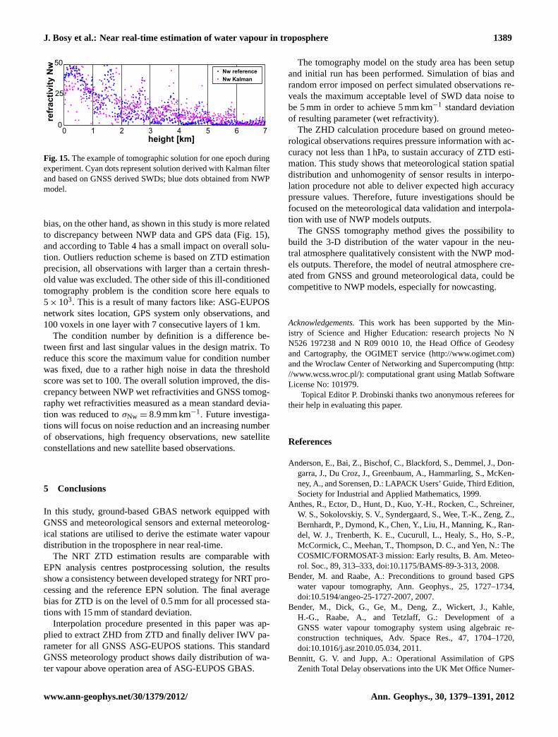
Fig. 15.The example of tomographic solution for one epoch duringexperiment. Cyan dots represent solution derived with Kalman filterand based on GNSS derived SWDs; blue dots obtained from NWPmodel.

bias, on the other hand, as shown in this study is more relatedto discrepancy between NWP data and GPS data (Fig.15),and according to Table4 has a small impact on overall solu-tion. Outliers reduction scheme is based on ZTD estimationprecision, all observations with larger than a certain thresh-old value was excluded. The other side of this ill-conditionedtomography problem is the condition score here equals to5×103. This is a result of many factors like: ASG-EUPOSnetwork sites location, GPS system only observations, and100 voxels in one layer with 7 consecutive layers of 1 km.

The condition number by definition is a difference be-tween first and last singular values in the design matrix. Toreduce this score the maximum value for condition numberwas fixed, due to a rather high noise in data the thresholdscore was set to 100. The overall solution improved, the dis-crepancy between NWP wet refractivities and GNSS tomog-raphy wet refractivities measured as a mean standard devia-tion was reduced toσNw = 8.9 mm km−1. Future investiga-tions will focus on noise reduction and an increasing numberof observations, high frequency observations, new satelliteconstellations and new satellite based observations.

5 Conclusions

In this study, ground-based GBAS network equipped withGNSS and meteorological sensors and external meteorolog-ical stations are utilised to derive the estimate water vapourdistribution in the troposphere in near real-time.

The NRT ZTD estimation results are comparable withEPN analysis centres postprocessing solution, the resultsshow a consistency between developed strategy for NRT pro-cessing and the reference EPN solution. The final averagebias for ZTD is on the level of 0.5 mm for all processed sta-tions with 15 mm of standard deviation.

Interpolation procedure presented in this paper was ap-plied to extract ZHD from ZTD and finally deliver IWV pa-rameter for all GNSS ASG-EUPOS stations. This standardGNSS meteorology product shows daily distribution of wa-ter vapour above operation area of ASG-EUPOS GBAS.

The tomography model on the study area has been setupand initial run has been performed. Simulation of bias andrandom error imposed on perfect simulated observations re-veals the maximum acceptable level of SWD data noise tobe 5 mm in order to achieve 5 mm km−1 standard deviationof resulting parameter (wet refractivity).

The ZHD calculation procedure based on ground meteo-rological observations requires pressure information with ac-curacy not less than 1 hPa, to sustain accuracy of ZTD esti-mation. This study shows that meteorological station spatialdistribution and unhomogenity of sensor results in interpo-lation procedure not able to deliver expected high accuracypressure values. Therefore, future investigations should befocused on the meteorological data validation and interpola-tion with use of NWP models outputs.

The GNSS tomography method gives the possibility tobuild the 3-D distribution of the water vapour in the neu-tral atmosphere qualitatively consistent with the NWP mod-els outputs. Therefore, the model of neutral atmosphere cre-ated from GNSS and ground meteorological data, could becompetitive to NWP models, especially for nowcasting.

Acknowledgements.This work has been supported by the Min-istry of Science and Higher Education: research projects No NN526 197238 and N R09 0010 10, the Head Office of Geodesyand Cartography, the OGIMET service (http://www.ogimet.com)and the Wroclaw Center of Networking and Supercomputing (http://www.wcss.wroc.pl/): computational grant using Matlab SoftwareLicense No: 101979.

Topical Editor P. Drobinski thanks two anonymous referees fortheir help in evaluating this paper.

References

Anderson, E., Bai, Z., Bischof, C., Blackford, S., Demmel, J., Don-garra, J., Du Croz, J., Greenbaum, A., Hammarling, S., McKen-ney, A., and Sorensen, D.: LAPACK Users’ Guide, Third Edition,Society for Industrial and Applied Mathematics, 1999.

Anthes, R., Ector, D., Hunt, D., Kuo, Y.-H., Rocken, C., Schreiner,W. S., Sokolovskiy, S. V., Syndergaard, S., Wee, T.-K., Zeng, Z.,Bernhardt, P., Dymond, K., Chen, Y., Liu, H., Manning, K., Ran-del, W. J., Trenberth, K. E., Cucurull, L., Healy, S., Ho, S.-P.,McCormick, C., Meehan, T., Thompson, D. C., and Yen, N.: TheCOSMIC/FORMOSAT-3 mission: Early results, B. Am. Meteo-rol. Soc., 89, 313–333,doi:10.1175/BAMS-89-3-313, 2008.

Bender, M. and Raabe, A.: Preconditions to ground based GPSwater vapour tomography, Ann. Geophys., 25, 1727–1734,doi:10.5194/angeo-25-1727-2007, 2007.

Bender, M., Dick, G., Ge, M., Deng, Z., Wickert, J., Kahle,H.-G., Raabe, A., and Tetzlaff, G.: Development of aGNSS water vapour tomography system using algebraic re-construction techniques, Adv. Space Res., 47, 1704–1720,doi:10.1016/j.asr.2010.05.034, 2011.

Bennitt, G. V. and Jupp, A.: Operational Assimilation of GPSZenith Total Delay observations into the UK Met Office Numer-

www.ann-geophys.net/30/1379/2012/ Ann. Geophys., 30, 1379–1391, 2012

1390 J. Bosy et al.: Near real-time estimation of water vapour in troposphere

ical Weather Prediction models, Mon. Weather Rev., 140, 2706–2719,doi:10.1175/MWR-D-11-00156.1, 2012.

Bevis, M., Businger, S., Herring, T., Rocken, C., Anthes, R., andWare, R.: GPS meteorology: Remote sensing of atmospheric wa-ter vapor using the global positioning system, J. Geophys. Res.,(D), 15787–15801, 1992.

Bevis, M., Businger, S., Chiswell, S., Herring, T., Anthes, R.,Rocken, C., and Ware, R.: GPS meteorology: Mapping zenithwet delays onto precipitable water, J. Appl. Meteorol., 33, 379–386, 1994.

BKG: BKG Ntrip Client (BNC) Version 2.5. Manual, FederalAgency for Cartography and Geodesy, Frankfurt, Germany,2011.

Boehm, J., Niell, A., Tregoning, P., and Schuh, H.: Global MappingFunction (GMF): A new empirical mapping function based onnumerical weather model data, Geophys. Res. Lett., 33, 15–26,doi:10.1029/2005GL025546, 2006.

Borkowski, A., Bosy, J., and Kontny, B.: Meteorological data anddetermination of heights in local GPS networks–preliminaryresults, Electronic Journal of Polish Agricultural Universities,Geodesy and Cartography, 5, 2002.

Bosy, J., Figurski, M., and Wielgosz, P.: A strategy for GPS dataprocessing in a precise local network during high solar activity,GPS Solutions, 7, 120–129, 2003.

Bosy, J., Oruba, A., Graszka, W., Leonczyk, M., and Ryczywol-ski, M.: ASG-EUPOS densification of EUREF Permanent Net-work on the territory of Poland, Reports on Geodesy, 2, 105–112,2008.

Bosy, J., Rohm, W., Borkowski, A., Kroszczynski, K., and Figurski,M.: Integration and verification of meteorological observationsand NWP model data for the local GNSS tomography, Atmos.Res., 96, 522–530,doi:10.1016/j.atmosres.2009.12.012, 2010a.

Bosy, J., Rohm, W., and Sierny, J.: The concept of the near realtime atmosphere model based on the GNSS and the meteorologi-cal data from the ASG-EUPOS reference stations, Acta Geodyn.Geomater., 7, 1–9, 2010b.

Boudouris, G.: On the index of refraction of air, the absorption anddispersion of centimeter waves by gases, J. Res. National Bureauof Standards, 67D, 631–684, 1963.

Dach, R., Hugentobler, U., Fridez, P., and Meindl, M.: Bernese GPSSoftware Version 5.0, Astronomical Institute, University of Bern,2007.

Dousa, J.: Evaluation of tropospheric parameters estimated in var-ious routine GPS analysis, Physics and Chemistry of the Earth,Parts A/B/C, 29, 167–175,doi:10.1016/j.pce.2004.01.011, 2004.

Dousa, J.: The impact of errors in predicted GPS orbits on zenithtroposphere delay estimation, GPS Solutions, 14, 229–239,doi:10.1007/s10291-009-0138-z, 2010a.

Dousa, J.: Precise Near Real-Time GNSS Analyses at GeodeticObservatory Pecny – Precise Orbit Determination and WaterVapour Monitoring, Acta Geodynamica et Geomaterialia, 7, 7–17, 2010b.

Flores, A., Ruffini, G., and Rius, A.: 4D tropospheric tomogra-phy using GPS slant wet delays, Ann. Geophys., 18, 223–234,doi:10.1007/s00585-000-0223-7, 2000.

Grejner-Brzezinska, D. A., Arslan, N., Wielgosz, P., and Hong, C.-K.: Network Calibration for Unfavorable Reference-Rover Ge-ometry in Network-Based RTK: Ohio CORS Case Study, J.Surveying Engineering, 135, 90–100,doi:10.1061/(ASCE)0733-

9453(2009)135:3(90), 2009.Heise, S., Dick, G., Gendt, G., Schmidt, T., and Wickert, J.: Inte-

grated water vapor from IGS ground-based GPS observations:initial results from a global 5-min data set, Ann. Geophys., 27,2851–2859,doi:10.5194/angeo-27-2851-2009, 2009.

Hirahara, K.: Local GPS tropospheric tomography, Earth PlanetsSpace, 52, 935–939, 2000.

Hodur, R.: The Naval Research Laboratory’s CoupledOcean/Atmospheric Mesoscale Prediction System, Mon.Weather Rev., 125, 1414–1430, 1997.

Jarvinen, H., Eresmaa, R., Vedel, H., Salonen, K., Niemela, S., andde Vries, J.: A variational data assimilation system for ground-based GPS slant delays, Q. J. Roy. Meteorol. Soc., 133, 969–980,doi:10.1002/qj.79, 2007.

Karabatic, A., Weber, R., and Haiden, T.: Near real-time es-timation of tropospheric water vapour content from groundbased GNSS data and its potential contribution to weathernow-casting in Austria, Adv. Space Res., 47, 1691–1703,doi:10.1016/j.asr.2010.10.028, 2011.

Kee, C., Parkinson, B. W., and Axelrad, P.: Wide Area DifferentialGPS, Navigation, 38, 123–146, 1991.

Kleijer, F.: Troposphere Modeling and Filtering for Precise GPSLeveling, Ph.D. thesis, Department of Mathematical Geodesyand Positioning, Delft University of Technology, Kluyverweg1, P.O. Box 5058, 2600 GB DELFT, The Netherlands, 260 pp.,2004.

Mendes, V. B.: Modeling the neutral-atmosphere propagation de-lay in radiometric space techniques, Ph.D. thesis, Deparment ofGeodesy and Geomatics Engineering Technical Reort No. 199,University of New Brunswick, Fredericton, New Brunswick,Canada, 1999.

Mervart, L.: Ambiguity resolution techniques in geodetic andgeodynamic applications of the Global Positioning System,Ph.D. thesis, Astronomical Institute, Druckerei Universitat Bern,Berne, Switzerland, geodatisch-geophysikalische Arbeiten in derSchweiz, Band 53, Schweizerische Geodatische Kommision,Institut fur Geodasie und Photogrammetrie, Eidg. TechnischeHochschule Zurich, Zurich, 1995.

Niell, A. E.: Global mapping functions for the atmosphere delay atradio wavelenghs, J. Geophys. Res., 101, 3227–3246, 1996.

Nilsson, T. and Gradinarsky, L.: Water Vapor Tomography Us-ing GPS Phase Observations: Simulation Results, IEEE Trans.Geosci. Remote Sens., 44, 2927–2941, 2006.

Perler, D., Geiger, A., and Hurter, F.: 4D GPS water vapor tomog-raphy: new parameterized approaches, J. Geodesy, 85, 539–550,doi:10.1007/s00190-011-0454-2, 2011.

Rankine, W. J. M. and Bamber, E. F.: Useful Rules and Tables Relat-ing to Mensuration, Engineering, Structures and Machines, Bib-lioBazaar, LLC, (reprint from 1876), 2009.

Rohm, W.: The precision of humidity in GNSS tomography, Atmos.Res., 107, 69–75,doi:10.1016/j.atmosres.2011.12.008, 2012.

Rohm, W. and Bosy, J.: Local tomography tropospheremodel over mountains area, Atmos. Res., 93, 777–783,doi:10.1016/j.atmosres.2009.03.013, 2009.

Rohm, W. and Bosy, J.: The verification of GNSS tropospheric to-mography model in a mountainous area, Adv. Space Res., 47,1721–1730,doi:10.1016/j.asr.2010.04.017, 2011.

van der Marel, H.: COST-716 demonstration project for the nearreal-time estimation of integrated water vapour from GPS,

Ann. Geophys., 30, 1379–1391, 2012 www.ann-geophys.net/30/1379/2012/

J. Bosy et al.: Near real-time estimation of water vapour in troposphere 1391

Physics and Chemistry of the Earth, Parts A/B/C, 29, 187–199,doi:10.1016/j.pce.2004.01.001, 2004.

Vedel, H. and Huang, X.-Y.: Impact of Ground Based GPS Data onNumerical Weather Prediction, J. Meteorol. Soc. Japan. Ser. II,82, 459–472, 2004.

Wickert, J., Michalak, G., Schmidt, T., Beyerle, G., Cheng, C.,Healy, S., Heise, S., Huang, C., Jakowski, N., Kohler, W.,Mayer, C., Offiler, D., Ozawa, E., Pavelyev, A. G., Rothacher,M., Tapley, B., and Arras, C.: GPS radio occultation: re-sults from CHAMP, GRACE and FORMOSAT-3/COSMIC,Terrestrial Atmospheric and Oceanic Sciences, 20, 35–50,doi:10.3319/TAO.2007.12.26.01(F3C), 2009.

Wielgosz, P., Cellmer, S., Rzepecka, Z., Paziewski, J., and Grejner-Brzezinska, D.: Troposphere modeling for precise GPS rapidstatic positioning in mountainous areas, Meas. Sci. Technol., 22,doi:10.1088/0957-0233/22/4/045101, 2011.

www.ann-geophys.net/30/1379/2012/ Ann. Geophys., 30, 1379–1391, 2012