Nearness relations in environmental space

Michael F Worboys

Department of Computer Science

Keele University, Staffordshire

UK ST5 5BG

Abstract

This paper presents an experiment with human subjects concerning the vague spatial

relation ‘near’ in environmental space. After the topic is introduced and relevant previous

work surveyed, the experiment is described. Three approaches to experimental analysis

are presented and discussed: nearness neighbourhoods as regions with broad boundaries,

fuzzy nearness and distance measures, and four-valued logic. Issues discussed in further

detail are the truth gap – truth glut hypotheses regarding the psychology of vague predi-

cates, and formal properties of the three-valued nearness relation. Conclusions are drawn

and directions for future work suggested.

1 Introduction

This paper reports work done with human subjects on the spatial relation ‘near’ in environ-

mental space. There is a need for formal theories of spatial representation and reasoning to be

cognitively plausible, that is properly guided by the way humans actually think about space.

There is now a considerable body of work, some reviewed below, on the topic of vagueness,

1

2

imprecision, uncertainty and indeterminacy of spatial observations and representations (see

(Burrough and Frank 1996) for a good anthology) . Formalisms that have been proposed in-

clude fuzzy sets and logic, rough sets, geostatistical techniques, and multi-valued logics. This

paper seeks to apply appropriate theories to data from human subjects nearness relations

between places with two purposes: to better understand how humans conceptualize nearness

and to test the fit of formal theories to human concepts.

Techniques for handling linguistic descriptions of space have applications that include

incorporation of linguistic terms in queries to a spatial database (including fuzzy spatial

footprints to retrieve information from a digital library), appropriate human-centred interfaces

to geospatial datasets, and automated navigation. Goodchild (Goodchild 2000) offers as an

example the case of a caller to an emergency dispatcher, where the efficient conversion of a

linguistic description of a location to a quantitative specification can be a matter of life and

death.

An environmental space is the space of “buildings, neighborhoods, and cities” (Montello

1993) and useful knowledge of it cannot usually be gained by one observation, but only by a

series of observations over time and from different locations in the space. Therefore, knowl-

edge of the space is gained by integrating knowledge gained from several ‘views’. Montello

distinguishes environmental space from geographical space by noting that in the latter, sym-

bolic representation such as maps are required to gain useful knowledge. For the purposes

of the work described in this paper, the space may be either environmental or geographical,

although in our experiment the subjects were specifically asked not to refer to maps to answer

the questions put to them.

This paper reports research on nearness and other ‘conceptual’ distance relations in a

particular environmental space: the campus of Keele University in England. Keele University

3

Campus comprises 600 acres of landscaped grounds to the west of the Potteries conurbation in

North Staffordshire. The Keele Campus was chosen for the experiment partly for convenience,

the author being an academic at Keele, but also for its size and its irregular configuration of

buildings, roads and areas (see Figure 1), thus providing interesting questions about distance

relations within it.

A key component of the reported research is an experiment with human subjects, all

members of Keele University, concerning the conceptualization of the nearness relation on

the Keele Campus. The following sections describe the experimental design and analysis of

results. The way that the experiment is set up allows us to gain insights into ‘conceptualized’

distances between places on the campus for the population of subjects. The analysis is all

population-based, and no attention has been paid in this paper to individual differences,

although the data will allow such analysis. Also, unlike some other work on nearness (see

Section 2), the analysis is not concerned with the detailed effects of topography (e.g. hills,

lines of sight and roads) on human perception of distance but on more broadly based effects

such as overall contextual factors such as scale.

The work introduces three approaches to analysis of the results of the experiment. These

are:

Approach A. Nearness neighbourhood regions with broad boundaries.

Approach B. Fuzzy nearness and distance measures.

Approach C. Higher-valued logics where conflicting views may be represented.

Each approach allows its own insight into the analysis of results.

Following a review of the relevant background literature in Section 2, the experiment

is described in Section 3 and analysed using the three approaches in Section 4. Further

4

discussion of the results is taken up in the remainder of the paper, which concludes with a

summary of the principal arguments and points to directions for future research.

2 Background

The experiment described below concerns nearness relations between places in an environ-

mental space. Nearness is a vague concept, in the technical sense that it conforms to two

generally accepted (Williamson 1994) properties:

1. Existence of borderline cases

2. Susceptibility to the sorites paradox

Context is very important when working with a concept such as nearness. However, in

a given context, we might believe that Oxford is near London but that Edinburgh is not.

However, the first property reveals itself when we move north from Oxford, through Banbury

to Birmingham, and so on. At some point we are likely to arrive at borderline places for

which we do not wish to commit whether the place is near or not near London. Vagueness is

that particular kind of imprecision where there are borderline cases for which it is difficult to

decide whether they are covered by the concept or not.

Refining the argument further, assume as before that the context determines that we are

certain that Oxford is near London. Now, move northwards one metre from Oxford – such

a small change in position surely cannot make any difference to the truth of our proposition

that we are near London. Now move north one more metre, and one more, and continue until

arrival in Edinburgh. At each stage the small change in position means that we maintain

the truth of the proposition that we are near London. At some point, we will be forced to

5

admit the contradictory nature of our belief set, arguing that we are near London while being

clearly not near to London. This is the second property of a vague concept or predicate.

Many works mainly in the philosophical literature, have provided general treatments of

vagueness. Keefe and Smith (Keefe and Smith 1996) have edited a useful anthology, and

Williamson (Williamson 1994) provides a comprehensive overview. An approach to reasoning

that avoids some of the difficulties inherent in the sorites paradox is provided by the super-

valuationary semantics of Kit Fine (Fine 1975). There is a smaller amount of research (e.g.

( Varzi 2001, Fisher 1997, Fisher 2000 ) that looks at vagueness in the context of geographic

space.

A major motivation for the work presented here is to parallel the work of Bonini et al.

(Bonini et al. 1999) on truth gap/glut theories of the psychology of vagueness. When asked

if a person is tall, you may not wish to commit yourself (tallness is a vague predicate and you

may be in the borderline region). Is your inability to commit due to lack of information (truth

gap) or too much and conflicting information (truth glut), or some other reason? Bonini and

colleagues addressed this question using concepts such as ‘being tall’, ‘being a mountain’,

‘being old’, ‘being late’, etc. They got at the question indirectly by dividing the group of

subjects into two, and asking one group a positive question and the other a negative question,

and determined whether there was an overlap or gap between the set of responses. The results

provided some evidence in favour of the truth gap theory of vagueness.

Work on the spatial relation ‘near’ can be traced back at least as far as Lundberg and Ek-

man (Lundberg and Eckman 1973). Denofsky (Denofsky 1976) noted problems in specifying

the inherently vague concept pair near–far. Work on qualitative spatial reasoning applied to

proximity includes ( Dutta 1990, Frank 1992, Hernandez et al. 1995). Application of fuzzy

logic techniques to representing spatial relations such as near are discussed by Robinson et

6

al. (Robinson et al. 1986). In (Robinson 1990), Robinson determines the meaning of ‘near’

using the surrogate variable ‘distance’ by means of a question-answer approach with human

subjects. The system ‘learns’ the concept ‘near’ by constructing a fuzzy set of the places near

the reference place. Robinson’s experiment has some similarity with the work reported in this

paper, but here no surrogate variable is used. In (Robinson 2000), Robinson took the dis-

cussion forward by using the same techniques to elicit individual differences among subjects

in the semantics of spatial relations such as nearness. The question of individual differences

was also taken up be Fisher and Orf (Fisher and Orf 1991), who worked with students on

the campus of Kent State University, USA. They identified three clusters among the sub-

jects, with quite different semantics for the spatial relations ‘near’ and ‘close’. Despite some

analysis of the personal characteristics of the subjects, they were unable to use these to give

a significant prediction of which cluster a subject belonged. Gahegan (Gahegan 1995) also

discusses experimental work on qualitative measures of proximity. His results indicate that

contextual factors important for judgements on nearness include connection paths between

places, scale, and ‘attractiveness’ of objects.

One of the approaches that we adopt in the experimental analysis is the use of a three-

valued logic, resulting in ‘nearness neighbourhoods’ of places that are regions with broad

boundaries. This 3-valued indeterminacy of location in the neighbourhood has been rep-

resented by several authors as a region with broad boundary, also known as the egg-yolk

diagram (Clementini and Felice, 1996a; Cohn and Gotts, 1996a,b; Schneider, 1996; Erwig and

Schneider, 1997; Clementini and Felice, 1997). Broad boundaries can be seen as a geomet-

ric model that approximate many different situations related to uncertainty. In a previous

paper (Worboys and Clementini 2001), some of these situations are enumerated as represen-

tations based on incomplete information, conflicting information, and changing information

7

of a dynamic phenomenon, as well as representations of inherently vague concepts (such as

nearness).

3 Nearness experiment

The experiment was conducted during the summer of 2000 using the Keele University Campus,

which comprises 600 acres of landscaped grounds to the west of the Potteries conurbation in

North Staffordshire, England. The broad purpose of the experiment was to gain information

about the way that humans think about the vague spatial relation of nearness in the context

of environmental space (Montello 1993). 22 human subjects were chosen, each of whom was

a member of university staff and had been working on the campus for some years and so was

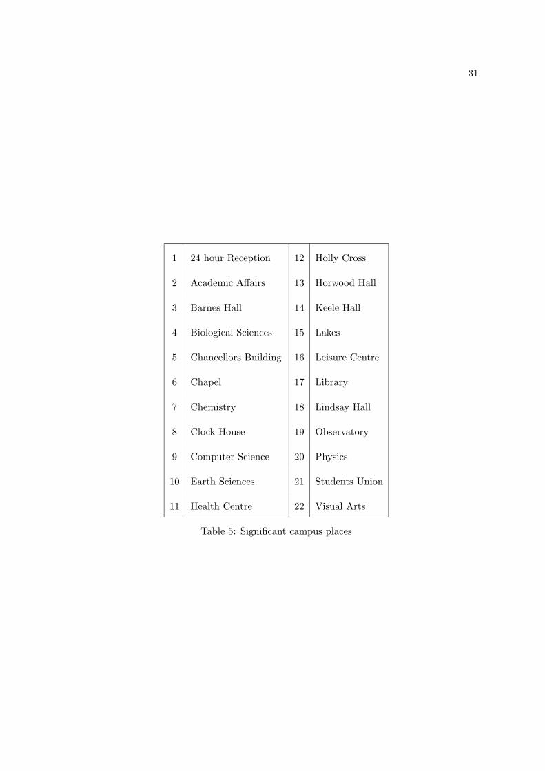
generally familiar with the environment. As a preliminary to the experiment, subjects were

asked to nominate ‘significant places’ on the campus (as many as they wished), votes were

counted and those locations with the most votes were selected. A list of significant places is

shown in Table , and a map of their positions on the campus is shown in Figure 1.

In the main phase of the experiment, the subjects were divided into two equal groups,

the truth group and falsity group. Each member of each group was then given a series of

questionnaires, one questionnaire for each of the significant places identified in the earlier

phase.

Each questionnaire concerned the location of a list of places with respect to a fixed place,

termed in this paper the reference place. Each questionnaire consisted of a heading that

identified the reference place and provided some instructions about what was required of the

subject. There followed a list of all the significant places with the exception of the reference

8

Figure 1: Significant campus places

place. The subjects had the option to tick or not tick each of the places in the list, depending

on their response to the instructions in the heading. The heading instructions depended on

whether the subject was in the truth group or falsity group, and are given below.

Instructions to the truth group: When is it true to say that a place is near [reference

place]? We’re interested in your view of the matter. Please indicate, by ticking the

places below, for which of the following places is it true to say that the place is near

[reference place].

Instructions to the falsity group: When is it false to say that a place is near [reference

place]? We’re interested in your view of the matter. Please indicate, by ticking the

places below, for which of the following places is it false to say that the place is near

[reference place].

Each subject in the truth and falsity groups completed one questionnaire for each of

the twenty two significant places playing the role of reference place. The questionnaires were

9

spaced at least one day apart and each questionnaire was collected before the next was issued.

In this way we tried to ensure that no explicit cross-referencing could be made. Subjects were

asked neither to deliberate too long or hard on the questions, nor to refer to campus maps

for the duration of the experiment.

4 Analysis of results

For each reference place, the total number of ticks awarded to each significant place in the

list by the truth and falsity groups respectively was calculated. The subjects were not asked

about the proximity relation of each reference place to itself, as we are assuming that a place

is near itself, by definition. Data was added by the experimenters to this effect (11 votes in

the truth column and 0 votes in the falsity column).

As an example, Table 1 shows the tallies for the case where the reference place is the

Library. The full set of results consists of two 22× 22 arrays, giving for each group and each

ordered pair of significant places, the sum of the number of votes from that group.

Three different approaches to analysis of the experimental data were taken: three-valued

logic and nearness neighbourhood regions with with broad boundaries; fuzzy distance and

fuzzy nearness neighbourhoods; four-valued and higher-valued logics. The first two ap-

proaches use techniques that merge the votes from the truth and falsity groups to either

a distance measure or a value in a three-valued logic, while the third approach leaves the

conflicts unresolved by moving from a three-valued logic to other multi-valued logics based

on Belnap’s four-valued logic (Belnap; Belnap 1976; 1977).

10

LIBRARY

Place Truth Falsity Place Truth Falsity

group group group group

24 hour Reception 4 4 Holly Cross 1 11

Academic Affairs 5 2 Horwood Hall 4 10

Barnes Hall 0 11 Keele Hall 8 2

Biological Sciences 5 4 Lakes 1 11

Chancellors Building 4 6 Leisure Centre 0 11

Chapel 10 0 Library 11 0

Chemistry 4 6 Lindsay Hall 2 8

Clock House 4 6 Observatory 0 11

Computer Science 1 10 Physics 5 5

Earth Sciences 7 0 Students Union 10 0

Health Centre 1 11 Visual Arts 1 10

Table 1: Library results

11

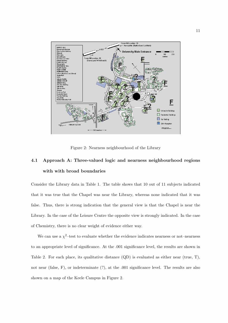
Figure 2: Nearness neighbourhood of the Library

4.1 Approach A: Three-valued logic and nearness neighbourhood regions

with with broad boundaries

Consider the Library data in Table 1. The table shows that 10 out of 11 subjects indicated

that it was true that the Chapel was near the Library, whereas none indicated that it was

false. Thus, there is strong indication that the general view is that the Chapel is near the

Library. In the case of the Leisure Centre the opposite view is strongly indicated. In the case

of Chemistry, there is no clear weight of evidence either way.

We can use a χ2–test to evaluate whether the evidence indicates nearness or not–nearness

to an appropriate level of significance. At the .001 significance level, the results are shown in

Table 2. For each place, its qualitative distance (QD) is evaluated as either near (true, T),

not near (false, F), or indeterminate (?), at the .001 significance level. The results are also

shown on a map of the Keele Campus in Figure 2.

12

LIBRARY

Place QD Place QD

24 hour Reception ? Holly Cross F

Academic Affairs ? Horwood Hall ?

Barnes Hall F Keele Hall ?

Biological Sciences ? Lakes F

Chancellors Building ? Leisure Centre F

Chapel T Library T

Chemistry ? Lindsay Hall ?

Clock House ? Observatory F

Computer Science F Physics ?

Earth Sciences ? Students Union T

Health Centre F Visual Arts F

Table 2: Nearness to the Library represented using three truth values

13

The data, as analysed in this way, provides a set of ‘nearness neighbourhoods’ of particular

places. Each neighbourhood is represented as a region with broad boundary, and part of the

overall purpose of the work is to check whether the formalisms for reasoning with regions

with broad boundaries (Clementini and Felice 1996b) or so-called egg-yolk regions (Cohn and

Gotts; Cohn and Gotts 1996a; 1996b) are cognitively plausible, in the sense of conforming to

human reasoning with such vague entities.

Limitations of this approach are that the boundaries between true, false and indeterminate

are themselves crisp, and also in our approach the boundaries will vary with the significance

level chosen. However, the method does provide a useful first approximation to representa-

tions of vagueness Section 6.4 below takes this approach further by considering nearness as a

special case of a similarity relation, and investigating how weak version of equivalence prop-

erties, weak symmetry and weak transitivity are satisfied by the qualitative nearness relation

constructed by this approach.

4.2 Approach B: Fuzzy nearness neighbourhoods and distance relations

This approaches refines Approach A by allowing a continuous measure of nearness between 0

and 1. Rather than a set with a broad boundary as the nearness neighbourhood of a place, we

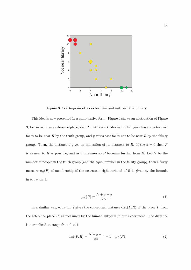
have a fuzzy neighbourhood. To illustrate the approach, Figure 3 shows a scattergram, where

votes cast for and against nearness of places to the reference place ‘the Library’ are measured

on the horizontal and vertical axes respectively. The areas of the circles plotted on the graph

are in direct proportion to the number of places with that pattern of votes. The conceptual

nearness of a place to the Library is indicated by its ‘nearness’ to the bottom left-hand corner

of the scattergram. Colours of the circles indicate the truth value of their nearness to the

Library, as in Approach A; green, yellow and red indicate T, ? and F, respectively.

14

Figure 3: Scattergram of votes for near and not near the Library

This idea is now presented in a quantitative form. Figure 4 shows an abstraction of Figure

3, for an arbitrary reference place, say R. Let place P shown in the figure have x votes cast

for it to be near R by the truth group, and y votes cast for it not to be near R by the falsity

group. Then, the distance d gives an indication of its nearness to R. If the d = 0 then P

is as near to R as possible, and as d increases so P becomes further from R. Let N be the

number of people in the truth group (and the equal number in the falsity group), then a fuzzy

measure µR(P ) of membership of the nearness neighbourhood of R is given by the formula

in equation 1.

µR(P ) =N + x − y

2N(1)

In a similar way, equation 2 gives the conceptual distance dist(P, R) of the place P from

the reference place R, as measured by the human subjects in our experiment. The distance

is normalized to range from 0 to 1.

dist(P, R) =N + y − x

2N= 1 − µR(P ) (2)

15

Figure 4: Calculating fuzzy nearness

Table 3 gives nearness and distance values for places with respect to the reference place

Library.

An interesting question is whether this distance function satisfies the properties of a metric

space, as given by equations 3, 4 and 5. Here, P denotes the set of all significant places.

∀P, Q ∈ P. dist(P, Q) = 0 if and only if P = Q (3)

∀P, Q ∈ P. dist(P, Q) = dist(Q, P ) (4)

∀P, Q, R ∈ P. dist(P, Q) + dist(Q, R) ≥ dist(P, R) (5)

Each place is fully near itself by definition, and so equation 3 holds by definition. Equation

4 is more interesting, as it is contributes to argument about whether locational similarity

relations are symmetric. We can note that the mean of |dist(P, Q)−dist(Q, P )|, where P and

16

LIBRARY

Place Nearness Distance Place Nearness Distance

24 hour Reception 0.50 0.50 Holly Cross 0.05 0.95

Academic Affairs 0.64 0.36 Horwood Hall 0.23 0.77

Barnes Hall 0.00 1.00 Keele Hall 0.77 0.23

Biological Sciences 0.55 0.45 Lakes 0.05 0.95

Chancellors Building 0.41 0.59 Leisure Centre 0.00 1.00

Chapel 0.95 0.05 Library 1.00 0.00

Chemistry 0.41 0.59 Lindsay Hall 0.23 0.77

Clock House 0.41 0.59 Observatory 0.00 1.00

Computer Science 0.09 0.91 Physics 0.50 0.50

Earth Sciences 0.82 0.18 Students Union 0.95 0.05

Health Centre 0.05 0.95 Visual Arts 0.09 0.91

Table 3: Nearness and distance measures relative to the Library

17

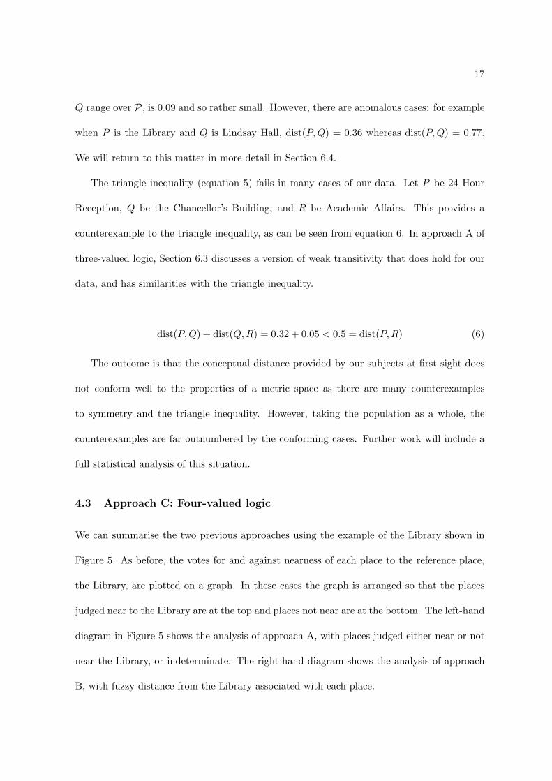
Q range over P, is 0.09 and so rather small. However, there are anomalous cases: for example

when P is the Library and Q is Lindsay Hall, dist(P, Q) = 0.36 whereas dist(P, Q) = 0.77.

We will return to this matter in more detail in Section 6.4.

The triangle inequality (equation 5) fails in many cases of our data. Let P be 24 Hour

Reception, Q be the Chancellor’s Building, and R be Academic Affairs. This provides a

counterexample to the triangle inequality, as can be seen from equation 6. In approach A of

three-valued logic, Section 6.3 discusses a version of weak transitivity that does hold for our

data, and has similarities with the triangle inequality.

dist(P, Q) + dist(Q, R) = 0.32 + 0.05 < 0.5 = dist(P, R) (6)

The outcome is that the conceptual distance provided by our subjects at first sight does

not conform well to the properties of a metric space as there are many counterexamples

to symmetry and the triangle inequality. However, taking the population as a whole, the

counterexamples are far outnumbered by the conforming cases. Further work will include a

full statistical analysis of this situation.

4.3 Approach C: Four-valued logic

We can summarise the two previous approaches using the example of the Library shown in

Figure 5. As before, the votes for and against nearness of each place to the reference place,

the Library, are plotted on a graph. In these cases the graph is arranged so that the places

judged near to the Library are at the top and places not near are at the bottom. The left-hand

diagram in Figure 5 shows the analysis of approach A, with places judged either near or not

near the Library, or indeterminate. The right-hand diagram shows the analysis of approach

B, with fuzzy distance from the Library associated with each place.

18

Figure 5: Approaches A and B applied to the Keele Library

Note that in both approaches A and B, only the vertical dimension in Figure 5 is being

utilized. However, consider the following examples from the figure:

24 Hour Reception Science near Library? Four votes in both the truth and falsity

groups.

Physics near Library? Five votes in both the truth and falsity groups.

In both previous approaches, the evaluation of nearness and conceptual distance is the

same for both items. Using Approach A:

QD(24 Hour Reception Science, Library) = QD(Physics, Library) = ? (7)

and using Approach B, from equation 2:

dist(24 Hour Reception Science, Library) = dist(Physics, Library) = 0.5 (8)

No distinction is made between the cases where there are few votes cast for either side and

where there are many votes cast either side. The first two approaches are unable to distinguish

between the cases where there is a dearth or surfeit of information. Belnap’s four-valued logic

19

Figure 6: Lattice of truth values in Belnap’s four-valued logic

(Belnap; Belnap 1976; 1977) does make such a distinction. Using such a formal approach has

the benefit that conflicting information can be maintained, represented and reasoned with in

the formalism. The essence of the approach is shown in Figure 6, which is a lattice of four

truth values: T, F, N, and B, where T and F are the usual classical values, and N (neither)

and B (both) represent dearth and surfeit of information in the indeterminate cases.

The similarity between Figures 5 and 6 is striking. We need to find some way of represent-

ing the indeterminate values from our data as either N or B values. As with the representation

of our data as three truth values, this further decomposition is to some extent arbitrary. We

have chosen the simple formula given in equation 9 below to represent the degree of conflict

between the votes x for and the votes against y the proposition. As before, let N be the

number of people in the truth group (and the equal number in the falsity group).

conflict(x, y) ::=min(x, y)

N(9)

To show one application of this approach, Figures 7 and 8 show the variation of conflict in

the subject’s judgements of a place’s nearness with the Euclidean distance of the place from

the reference place, in this case the Library and Lindsay Hall, respectively. As one would

expect, the conflict is highest for those places whose qualitative distance from the reference

20

Figure 7: Variation of level of conflict with Euclidean distance from the Library

place is indeterminate.

To reduce to four values as in Belnap’s system, we need to find some way of assigning

the indeterminate from the 3-valued logic (Approach A) to B or N. This is done in a fairly

arbitrary way by giving a value K such that if conflict(x, y) > K, assign truth value B to

(x, y), otherwise assign N. In the case of this experiment, we choose K = 0.25, roughly midway

between 0 and 0.5, the range of almost all of the conflicts in the dataset. Table 4 gives the

assignment of truth values in relation to the Library.

Both the choice of conflict function and particularly the choice of value for K have an

unsatisfactory degree of arbitrariness. However, consideration of the N-B dimension in the

data is clearly important, as will be seen in Section 5. By consideration of the full 12×12

lattice of voting pairs, we can eliminate both kinds of arbitrariness. In this case, the logic

is based on an extension of the Belnap 4-valued lattice of truth values to a multi-valued De

Morgan lattice (Font 1997). This is the subject of ongoing work. For now, we explore in

Section 5one direction in which consideration of the N-B dimension provides insight into the

21

Figure 8: Variation of level of conflict with Euclidean distance from Lindsay Hall

LIBRARY

Place QD Place QD

24 hour Reception B Holly Cross F

Academic Affairs N Horwood Hall B

Barnes Hall F Keele Hall N

Biological Sciences B Lakes F

Chancellors Building B Leisure Centre F

Chapel T Library T

Chemistry B Lindsay Hall N

Clock House B Observatory F

Computer Science F Physics B

Earth Sciences N Students Union T

Health Centre F Visual Arts F

Table 4: Nearness to the Library represented using four truth values

22

truth-gap, truth-glut theories of the psychology of vagueness.

5 Truth gap or truth glut?

An initial motivation for this work was to follow up the paper of Bonini et al. (Bonini et al.

1999) that tested hypotheses concerning the psychological origin of vagueness. Consider the

proposition ‘Keele Hall is near the Library’. We can see by reference to Table 2 that this

was considered to be a borderline case of nearness, and represented in three-valued logic as

indeterminate. If we are in this borderline between definitely near and definitely not near,

then there are at least two possible psychological interpretations.

Truth gap: Keele Hall is neither near nor not near the Library.

Truth glut: Keele Hall is both near and not near the Library.

The experiment described in Section 3 can be used to provide evidence relating to the

above positions. Consider the data concerning nearness to the Keele Library (Table 2 and

Figure 2). This may be plotted as a scattergram as in Figure 3, discussed in Section 4.2.

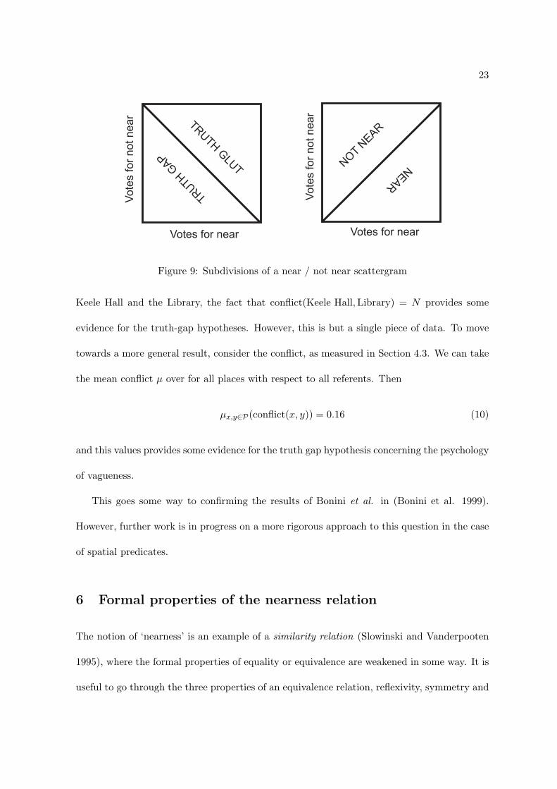
We have seen in the previous Section how such a scattergram may be broadly divided into

four regions (see Figure 9). The bottom right corner contains places that are near to the

Library (large majority of votes cast for nearness) while the top left corner contains places

that are not considered near to the Library (large majority of votes cast for not-nearness).

The bottom left corner contains places for which there are few votes either way (truth gap)

while the top right contains places for which there are large numbers of votes indicating both

nearness and not-nearness (conflict or truth glut).

By reference to Figure 3, we can see with the Library data that there is a general tendency

away from the top right area, and so some pictorial evidence for truth gap. In the case of

23

Figure 9: Subdivisions of a near / not near scattergram

Keele Hall and the Library, the fact that conflict(Keele Hall, Library) = N provides some

evidence for the truth-gap hypotheses. However, this is but a single piece of data. To move

towards a more general result, consider the conflict, as measured in Section 4.3. We can take

the mean conflict µ over for all places with respect to all referents. Then

µx,y∈P(conflict(x, y)) = 0.16 (10)

and this values provides some evidence for the truth gap hypothesis concerning the psychology

of vagueness.

This goes some way to confirming the results of Bonini et al. in (Bonini et al. 1999).

However, further work is in progress on a more rigorous approach to this question in the case

of spatial predicates.

6 Formal properties of the nearness relation

The notion of ‘nearness’ is an example of a similarity relation (Slowinski and Vanderpooten

1995), where the formal properties of equality or equivalence are weakened in some way. It is

useful to go through the three properties of an equivalence relation, reflexivity, symmetry and

24

transitivity, and note in what way the Keele campus experiment is able to usefully comment

on these properties. We will use the three truth values T, F and ?, as in Section 4.1. Let P

be the set of significant places on the Keele campus, and let ν be the three-valued nearness

relation on P, as defined above. Evaluation of ν to true, false or indeterminate is shown in our

formalism as xνx = T , xνx = F , and xνx =?, respectively. Let ρ be an arbitrary classical,

two-valued relation on P.

6.1 Reflexivity

For classical two-valued relations, the reflexive property is given by equation 11.

∀x ∈ P. xρx (11)

In this work, where ν is three-valued, we can say by definition that each place is near to itself,

and so we modify the reflexivity property as in equation 12.

∀x ∈ P. xνx = T (12)

6.2 Weak symmetry

A two-valued relation ρ is symmetric if equation 13 is valid.

∀x, y ∈ P. xρy implies yρx (13)

With nearness, it is not immediately clear from intuition whether the symmetry condition

holds or not. At first glance it appears that nearness is symmetrical; after all, we often say that

two places are near each other without indicating the direction in which the relation applies.

However, it is not hard to come up with examples where symmetry is highly questionable.

Take the case of Keele and Stoke (the nearest city, about 10 miles from Keele). From Stoke’s

25

point of view, Keele is a village within its environs, and so it is perfectly reasonable to think

of Keele as being near Stoke. On the other hand, from the parochial view of Keele, and

thinking at the scale of the campus, it is harder to think of Stoke as being near Keele. (There

are clearly senses in which Keele is near / not near Stoke, and Stoke is near / not near Keele

– we are going for balances of opinion here). So it is possible to find counterexamples to the

symmetry property for nearness.

In the case of our experiment, there are many counterexamples to equation 13. For exam-

ple, at the 0.001 significance level, the Chapel is near Academic Affairs but it is indeterminate

whether or not Academic Affairs is near the Chapel. However, at the 0.001 significance level,

and at any higher significance level, there are no cases where place x is near place y but y is

not near x. So we can formulate a weak version of symmetry, shown by equation 14 that is

valid for all places in our experiment at levels of significance greater than or equal to 0.001.

∀x, y ∈ P. xνy = T implies yνx �= F (14)

Notice that equation 14 implies equation 15.

∀x, y ∈ P. xνy = F implies yνx �= T (15)

6.3 Weak transitivity

A two-valued relation ρ is transitive if equation 16 is valid.

∀x, y, z ∈ P. (xρy and yρz) implies xρz (16)

As with symmetry, in our experiment, there are many counterexamples to equation 16. For

example, at the 0.001 significance level, the Students’ Union is near the Chapel and the Chapel

is near Academic Affairs, but it is indeterminate whether or not the Students’ Union is near

26

Academic Affairs. However, at the 0.001 significance level, and at any higher significance

level, there are no cases where place x is near place y and y is near z but x is not near z.

So we can formulate a weak version of transitivity, shown by equation 17 that is valid for all

places in our experiment at levels of significance greater than or equal to 0.001.

∀x, y, z ∈ P. (xνy = T and yνz = T ) implies (xνz �= F ) (17)

6.4 Nearness as similarity

Equations 11, 14, 17 provide a weakened version of equivalence that we might term ‘similarity’.

Similarity relations are described in the literature (e.g. Nieminen 1988, Polkowski et al. 1995,

Slowinski and Vanderpooten 1995) as reflexive relations in which symmetry and transitivity

are relaxed in some way. Our experiment has demonstrated many counterexamples to strong

symmetry and transitivity.

With regard to symmetry, weak symmetry implies a directionality to a similarity relation,

as with Tversky (Tversky 1997) and the example ‘a son resembles his father’. In this example,

the son and father play differing roles in the relation, the son being the subject and father the

referent. The inverse relation that ‘a father resembles his son’ is clearly more problematical.

For nearness, the subject–referent dichotomy plays a dominant role in that the referent creates

the scale in which the relation has context. This can be seen by returning to the data in Section

4.2.

Let P be the Library and Q be Lindsay Hall. Then, dist(P, Q) = 0.36 whereas dist(P, Q) =

0.77. What is the reason for the large asymmetry in the distance relationship? We get a strong

sense of what is going on if we plot the fuzzy distance relationship between places against

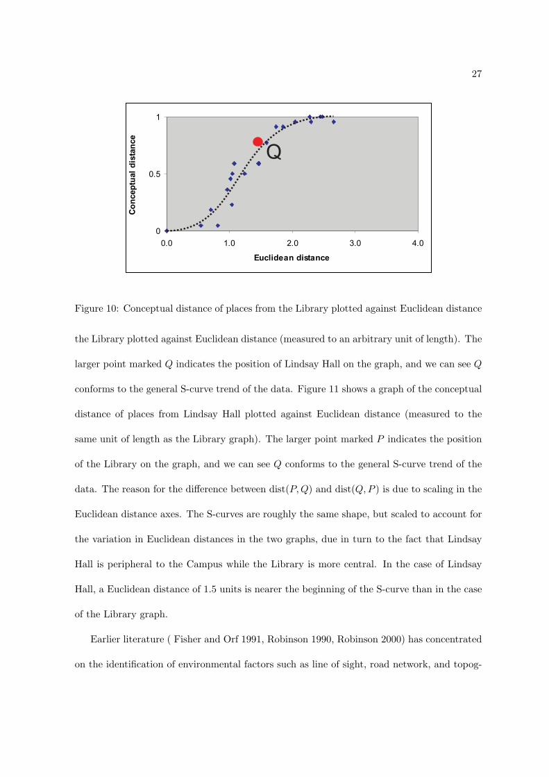
their Euclidean distances. Figure 10 shows a graph of the conceptual distance of places from

27

Figure 10: Conceptual distance of places from the Library plotted against Euclidean distance

the Library plotted against Euclidean distance (measured to an arbitrary unit of length). The

larger point marked Q indicates the position of Lindsay Hall on the graph, and we can see Q

conforms to the general S-curve trend of the data. Figure 11 shows a graph of the conceptual

distance of places from Lindsay Hall plotted against Euclidean distance (measured to the

same unit of length as the Library graph). The larger point marked P indicates the position

of the Library on the graph, and we can see Q conforms to the general S-curve trend of the

data. The reason for the difference between dist(P, Q) and dist(Q, P ) is due to scaling in the

Euclidean distance axes. The S-curves are roughly the same shape, but scaled to account for

the variation in Euclidean distances in the two graphs, due in turn to the fact that Lindsay

Hall is peripheral to the Campus while the Library is more central. In the case of Lindsay

Hall, a Euclidean distance of 1.5 units is nearer the beginning of the S-curve than in the case

of the Library graph.

Earlier literature ( Fisher and Orf 1991, Robinson 1990, Robinson 2000) has concentrated

on the identification of environmental factors such as line of sight, road network, and topog-

28

Figure 11: Conceptual distance of places from Lindsay Hall plotted against Euclidean distance

raphy, as explanations for variations in correlation between nearness and Euclidean distance.

The experiment reported in this paper shows the importance of scale factors introduced by

the context of the reference place. Another factor, also not considered here, is the relative im-

portance of the reference place compared with other places in the space. The work of Sorrows

and Hirtle (Sorrows and Hirtle 1999) on landmarks on the Pittsburgh campus takes account

of this. An underlying assumption in the experiment described in this paper is that no places

are inherently considerably more dominant than others. Certainly the Keele Campus has

nothing equivalent to Pittsburgh’s Cathedral of Learning.

Moving now to transitivity, for a similarity relation, transitivity is clearly too strong.

Small differences will eventually be propagated to something significant. So, in the example

of Luce (Luce 1956) with cups of coffee, cup A has no sugar and is judged similar in taste to

cup B with a small spoonful of sugar, and B is judged similar to C with a larger spoonful

of sugar. However, A and C may be judged dissimilar. Most discussions of similarity relax

transitivity only (e.g. Nieminen 1988, Polkowski et al. 1995). However, the above discussion

29

and our experiment show that symmetry may also need to be relaxed, as in (Slowinski and

Vanderpooten 1995)

7 Conclusions and future directions

This paper has sought to show how formal theories of vague spatial relations, can be properly

and usefully applied in a real situation involving human subjects. We have worked with the

inherently vague notion of nearness, deliberately specifying the minimum context required

to make a realistic scenario for our subjects to conceptualize about. We have shown how

three-valued logic, or its equivalent as regions with broad boundary can be applied to near-

ness, and that the resulting similarity relation has weak equivalence properties. We have

proposed a fuzzy membership function for nearness neighbourhoods of places and shown that

its related fuzzy distance function is rather far from having the properties of a metric space.

We investigated higher-valued logics, especially Belnap’s four-valued logic, as means to rep-

resent degrees of conflict in the experimental data, and showed that the experiment tended

to support the truth-gap view of the psychology of vagueness.

The work has raised several interesting issues for future investigation and some of these

are listed below.

• Semantics of logical operations with vague spatial predicates. For example, can we

form nearness neighbourhood of places P and Q (however that is interpreted) from the

nearness neighbourhood of place P and the nearness neighbourhood of place Q? Does

it correspond to one of the egg-yolk operations?

• Construction of a weak neighbourhood topology from the experimental data.

30

• Identification of useful landmarks for navigation from the experimental data. We have

ongoing work applying data mining techniques on rough sets to answer this question.

• Replication of the experiment with the same and different environmental spaces, to

detect commonalities.

• Consideration of the De Morgan lattice as a less ‘lossy’ representation of the experi-

mental data.

• Further investigation and statistical testing for conflict, including investigation of the

spatial characteristics of the conflict function.

8 Acknowledgements

The author is grateful for early discussions with Peter Jones on appropriate statistical meth-

ods, and to Matt Duckham for help with the analysis and useful discussions of many of

the ideas. The work was supported by the UK Engineering and Physical Sciences Research

Council grant ‘Vagueness, uncertainty and granularity in spatial information system’.

References

Belnap N., 1976. How computers should think. In Contemporary Aspects of Philosophy ,

edited by G. Ryle, pp. 30–56 (Boston: Oriel Press).

Belnap N., 1977. A useful four-valued logic. In Modern Uses of Multiple-valued Logic, edited

by J. Dunn and G. Epstein, pp. 8–37 (Dordrecht-Boston: Reidel).

Bonini N., Osherson D., Viale R., and Williamson T., 1999. On the psychology of vague

predicates. Mind and Language, 14, 373–393. Oxford: Blackwell.

31

1 24 hour Reception 12 Holly Cross

2 Academic Affairs 13 Horwood Hall

3 Barnes Hall 14 Keele Hall

4 Biological Sciences 15 Lakes

5 Chancellors Building 16 Leisure Centre

6 Chapel 17 Library

7 Chemistry 18 Lindsay Hall

8 Clock House 19 Observatory

9 Computer Science 20 Physics

10 Earth Sciences 21 Students Union

11 Health Centre 22 Visual Arts

Table 5: Significant campus places

32

Burrough P. and Frank A., editors, 1996. Geographic Objects with Indeterminate Boundaries.

GISDATA 2 (Taylor & Francis).

Clementini E. and Felice P.D., 1996a. An algebraic model for spatial objects with inde-

terminate boundaries. In Geographic Objects with Indeterminate Boundaries, edited by

P. Burrough and A. Frank, GISDATA Series, pp. 155–169 (London: Taylor & Francis).

Clementini E. and Felice P.D., 1996b. An algebraic model for spatial objects with inde-

terminate boundaries. In Geographic Objects with Indeterminate Boundaries, edited by

P. Burrough and A. Frank, pp. 155–169 (London: Taylor & Francis).

Clementini E. and Felice P.D., 1997. Approximate topological relations. International Journal

of Approximate Reasoning , 16, 173–204.

Cohn A. and Gotts N., 1996a. The ‘egg-yolk’ representation of regions with indeterminate

boundaries. In Geographic Objects with Indeterminate Boundaries, edited by P. Burrough

and A. Frank, pp. 171–187 (London: Taylor & Francis).

Cohn A. and Gotts N., 1996b. Representing spatial vagueness: A mereological approach. In

Principles of Knowledge Representation and Reasoning: Proc 5th International Conference

(KR96) (San Francisco: Morgan Kaufmann).

Denofsky M., 1976. How near is near? AI Memo 344, MIT AI Lab, Cambridge, MA.

Dutta S., 1990. Qualitative spatial reasoning: A semi-quantitative approach using fuzzy

logic. In Design and Implementation of Large Spatial Databases, edited by A. Buchmann,

O. Gunther, T. Smith, and Y.F. Wang, pp. 345–364 (Berlin: Springer Verlag).

Erwig M. and Schneider M., 1997. Vague regions. In Advances in Spatial Databases - Fifth

33

International Symposium, SSD’97 , edited by M. Scholl and A. Voisard, volume 1262 of

Lecture Notes in Computer Science, pp. 298–320 (Berlin: Springer Verlag).

Fine K., 1975. Vagueness, truth and logic. Synthese, 30, 265–300.

Fisher P., 1997. The pixel: a snare and a delusion. International Journal of Remote Sensing ,

18(3), 679–685.

Fisher P., 2000. Sorites paradox and vague geographies. Fuzzy Sets and Systems, 113(1),

7–18.

Fisher P. and Orf T., 1991. An investigation of the meaning of near and close on a university

campus. Computers, Environment and Urban Systems, 15, 23–25.

Font J., 1997. Belnap’s four-valued logic and De Morgan lattices. L.J of the IGPL, 5(3),

413–440.

Frank A., 1992. Qualitative spatial reasoning about distances and directions in geographic

space. Journal of Visual Languages and Computing , 3, 343–371.

Gahegan M., 1995. Proximity operators for qualitative spatial reasoning. In Spatial Infor-

mation Theory: A Theoretical Basis for GIS , edited by A. Frank and W. Kuhn, Lecture

Notes in Computer Science 988, pp. 31–44 (Berlin: Springer Verlag).

Goodchild M., 2000. GIS and transportation. GeoInformatica, 4(2), 127–140.

Hernandez D., Clementini E., and Felice P.D., 1995. Qualitative distances. In Spatial Infor-

mation Theory: A Theoretical Basis for GIS , edited by A. Frank and W. Kuhn, Lecture

Notes in Computer Science 988, pp. 45–58 (Berlin: Springer Verlag).

34

Keefe R. and Smith P., editors, 1996. Vagueness: A Reader (Cambridge MA: MIT Press).

ISBN 0262112256.

Luce R., 1956. Semi-orders and a theory of utility discrimination. Econometrica, 24.

Lundberg U. and Eckman G., 1973. Subjective geographic distance: A multidimensional

comparison. Psychometrika, 38(1), 113–122.

Montello D., 1993. Scale and multiple psychologies of space. In Spatial Information Theory:

A Theoretical Basis for GIS , edited by A. Frank and I. Campari, volume 716 of Lecture

Notes in Computer Science, pp. 312–321 (Berlin: Springer-Verlag).

Nieminen J., 1988. Rough tolerance equality. Fundamenta Informaticae, 11(3), 289–296.

Polkowski L., Skowron A., and Zytkow J., 1995. Tolerance based rough sets. In Soft Com-

puting: Rough Sets, Fuzzy Logic, Neural Networks, Uncertainty Management , edited by

T. Lin and A. Wildberger, pp. 55–58 (San Diego: Simulation Councils).

Robinson V., 1990. Interactive machine acquisition of a fuzzy spatial relation. Computers &

Geosciences, 16(6), 857–872.

Robinson V., 2000. Individual and multipersonal fuzzy spatial relations acquired using human-

machine interaction. Fuzzy Sets and Systems, 113, 133–145.

Robinson V., Blaze M., and Thongs D., 1986. Representation and acquisition of a natural

language relation for spatial information retrieval. In Proceedings SDH’86 , volume 951, pp.

472–487 (International Geographical Union).

Schneider M., 1996. Modelling spatial objects with undetermined boundaries using the

35

realm/rose approach. In Geographic Objects with Indeterminate Boundaries, edited by

P. Burrough and A. Frank, pp. 141–152 (London: Taylor & Francis).

Slowinski R. and Vanderpooten D., 1995. Similarity relations as a basis for rough

approximations. ICS Research Report 53/95, Warsaw University of Technology,

ftp://ftp.ii.pw.edu.pl/pub/Rough.

Sorrows M. and Hirtle S., 1999. The nature of landmarks for real and electronic spaces. In

Spatial Information Theory , edited by C. Freksa and D. Mark, volume 1661 of Lecture

Notes in Computer Science, pp. 37–50 (Berlin: Springer-Verlag).

Tversky A., 1997. Features of similarity. Psychological Review , 84(4), 327–352.

Varzi A., 2001. Vagueness in geography. Philosophy & Geography . Forthcoming.

Williamson T., 1994. Vagueness (London: Routledge).

Worboys M. and Clementini E., 2001. Integration of imperfect spatial information. Journal

of Visual Logic and Programming , 12. Forthcoming.