Negative Externalities

David Levinson

Motivation

• To measure externalities as a function of usage

• To enable the evaluation of the “Full Cost” of different modes under different circumstances

• To measure the costs consistently (in $/pkt) to compare fairly

Overview

• What are externalities• Key Issues• Our approach to the problem• Cost by cost discussion• Summary

Private Cost vs. Social Cost

• The purpose of distinguishing private and social cost is to correct for real resource misallocation from economic agents actions which impose a cost (or benefit) on others in the market. The market provides no incentive for agents to take account of their actions.

• The difference between private and social cost is that in making a decision a private individual will take account of the costs they face but will not consider the impact of their decision on others which may, in fact. impose a cost upon them. If this occurs an externality will misallocate resources since the economic agents is not forced to pay the cost they impose or does not receive any compensation for the benefits which they confer.

Externality• An externality is that situation in

which the actions of one agent imposes a benefit or cost on another economic agent who is not party to a transaction.

• Externalities are the difference between what parties to a transaction pay and what society pays

• A pecuniary externality, increases the price of a resource and therefore involves only transfers,

• A technical externality exhibits a real resource effect. A technical externality can be an external benefit (positive) or an external disbenefit (negative).

• Examples:– negative externalities

(external disbenefits) are air pollution, water pollution, noise, congestion.

– positive externalities (external benefits) are bees from apiary pollinating fruit trees and orchards supplying bees with nectar for honey.

Source of the Problem

• The source of externalities is the poorly defined property rights for an asset which is scarce. For example, no one owns the environment and yet everyone does. Since no one has property rights to it, no one will use it efficiently and price it. Without prices people treat it as a free good and do not cost it in their decision making. Overfishing can be explained in the same way.

• We want that amount of the externality which is only worth what it costs. Efficiency requires that we set the price of any asset >0 so the externality is internalized. If the price is set equal to the marginal social damages, we will get a socially efficient amount of the good or bad. Economic agents will voluntarily abate if the price is non-zero.

Coase Theorem

• The Coase Theorem states that in the absence of transaction costs, all allocations of property are equally efficient, because interested parties will bargain privately to correct any externality. As a corollary, the theorem also implies that in the presence of transaction costs, government may minimize inefficiency by allocating property initially to the party assigning it the greatest utility.

Pareto Optimality

• A change that can make at least one individual better off, without making any other individual worse off is called a Pareto improvement: an allocation of resources is Pareto efficient when no further Pareto improvements can be made.

What is the Optimal Amount of Externality

• 0?• Why / Why Not? [____]

Full Cost (FC) Model• FC = (CUT - TU) + CI + CE + CN + CA + CT

– User Costs (CU), • Total costs borne by users (CUT).

– cost of vehicle ownership (as measured by depreciation)– the cost of operating and maintaining the vehicle (including

gas, tires, repairs and such). • User Transfers (TU) = (infrastructure, accident and safety)

– Infrastructure Costs (CI), – Environmental Costs (CE), – Noise Costs (CN), – Accident and Safety Costs (CA), and – Time Costs (CT).

Key Issues

• “Externalities” are Inputs to Production System. Clean Air, Quiet, Safety, Freeflow Time are used to produce a trip.

• The System has boundaries: Direct effects vs. Indirect effects

• Double Counting must be avoided

Selection of Externalities• Criteria: Direct Effects• Not Internalized in Capital or Operating

Costs• External to User (not necessarily to

system)• Result: Noise, Air Pollution, Congestion,

Accidents• Not: Water Pollution, Parking, Defense ...

Approach

AirHighway Noise

Air Pollution

Congestion

Accidents

Measureme

nt Generation

Valuation

Integration

Noise: Measurement

• Noise: Unwanted Sound

• dB(A) = 10 log (P2/Pref)

• P: Pressure, Pref: queitest audible sound

• NEF: Noise Exposure Forecast is a function of number (frequency) of events and their loudness.

Noise: Generation

• Amount of noise generated is a function of traffic flow, speed, types of traffic.

• Additional vehicles have non-linear effect: e.g. 1 truck = 80 db, 2 trucks = 83 db, but sensitivity to loudness also rises

• Noise decays with distance

Noise: Valuation• Hedonic Models: Decline of Property

Values with Increase in Noise --> Noise Depreciation Index (NDI).

• Average NDI from many highway and airport studies is 0.62. For each unit increase in dB(A), there is a 0.62% decline in the price of a house

Noise: Integration• Noise Cost Functions ($/pkt) :

f(Quantity of Noise, House Values, Housing Density, Interest Rates)

• Using “reasonable” assumption, this ranges from $0.0001/vkt - $0.0060/vkt for highway. Best guess = $0.0045/pkt.

• For air, about the same, $0.0043/pkt.

Air Pollution: Measurement

• Air Pollution Problems: Smog, Acid Rain, Ozone Depletion, Global Climate Change.

• EPA “Criteria” Pollutants: HC (a.k.a. VOC, ROG), NOx, CO, SOx, PM10

• Other Pollutants: CO2

Air Pollution Generation

• Comparison of Modes

Mode Pax km HC kg,M

(gm/pkt)

COkg,M

(gm/pkt)

NOxkg, M(gm/pkt)

C,TonM

(gm/pkt) Highways 5.4 x1012 5,118

(0.95)32,690

(6.053)5,945(1.11)

263.2(46)

Jets 5.8 x1011 54(0.093)

163(0.28)

72.7(0.13)

59.2(100)

Total Transport

6,409 39,972 7,918

Total All Sources

18,536 60,863 19,890

Air Pollution: Valuation

• Local Health Effects, Material and Vegetation Effects, Global Effects

• Greatest Uncertainty in Global Effects, Proposed “Carbon Tax” have 2 orders of magnitude differences

Air Pollution: IntegrationPollutant Air Cost

($/pkt)

Highway Costs($/vkt)

PM10 --- $0.000085

SOx --- $0.000315

HC $0.0001530 $0.003850

CO $0.0000018 $0.000049

NOx $0.0001700 $0.001000

Carbon $0.0005800 $0.000260

TOTAL $0.0009048 $0.005559

Congestion: Measurement

• Time: Congested, Uncongested• Congested Time Increases as Flow

Approaches, Exceeds “Capacity”• Uncongested Time: Freeflow Time

+ Schedule Delay

Congestion: Generation

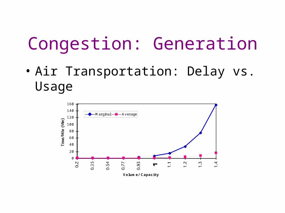
• Air Transportation: Delay vs. Usage

0

20

40

60

80

100

120

140

160

Volume/ Capacity

Marginal Average

Congestion: Valuation

• Value of Time is a function of mode, time of day, purpose, quality of service, trip-maker.

• Wide range, typically $50/hr air, $30/hr car. (Business Trips more valuble than Personal Trips).

• On other hand, average hourly PCI rate (40 hour week) gives $10/hr

Congestion: Integration

• Time Cost Functions:

TC = VoT Qh ( Lf/ Vf + a (Qh / Qho)b)• highway: a=0.32, b=10• air: a=2.33, b=6

Accidents: Measurement

• Number of Accidents by Severity• Multiple Databases (NASS, FARS)• Multiple Agencies (NHTSA, NTSB),

+ states and insurance agencies• Inconsistent Classification• Non-reporting

Accidents: Generation

• Accident Rates, Functions• Highway: Accident Rate =

f(urban/rural, onramps, auxiliarly lanes, flow, queueing)

• Air: Accident Rate = f( type of aircraft)

Accidents: Valuation

• Value of Life:• average of studies $2.9 M• average of highway studies $2.7 M• Cost of Non-fatal accident depends

on property damage, injury (degree of functional life lost, police costs, etc.)

Accidents: Integration

• Highway Accident Costs estimates range from $0.002 - $0.09/pkt. Our estimate is $0.02/pkt.

• Urban / rural tradeoff. Urban more but less severe accidents.

• Air Accident Costs $0.0005/pkt.

Summary: $/pkt

Summary: Conceptual

• High Uncertainty About Valuation• Costs Vary with Usage• Accounting, Difficult, but necessary

to avoid double counting.

Theoretical Framework• To establish optimal

emission level s for pollution, congestion or any other externality consider the following framework.

• Let ei = total emission from source i.

• Let Zi = amount of emission at source i in an uncontrolled state.

• Let Ai = Zi - ei be the abatement at source i. (1)

• Note if Ai = 0, Zi = ei or actual emissions equal the maximum amount possible.

TCi

A

= ci

( Ai

) = ci

( Zi

– ei

) (2)

is the cost of abatement with

cA

'

> 0 and cA

"

≥ 0

and

TD = f ( e ) (3)

is the damage function at receptor points

Solution

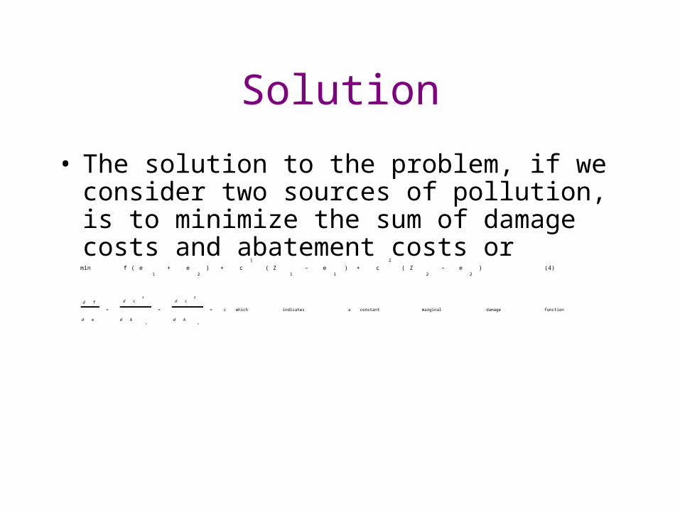
• The solution to the problem, if we consider two sources of pollution, is to minimize the sum of damage costs and abatement costs or

min f ( e1

+ e2

) + c

1

( Z1

– e1

) + c

2

( Z2

– e2

) (4)

d f

d e

=

d c1

d A1

=

d c2

d A2

= c which indicates a constant marginal damage function

Graphically

$/e

e

1

e2

E

$/e $/e

0 0 0

Source 1Source 2 Aggregate

Pollution

-

dc

1

de

1

-

dc

2

de

2

E*e*

1

e*

2

df

de

df

de

dc

i

de

i

∑

Optimal Amount

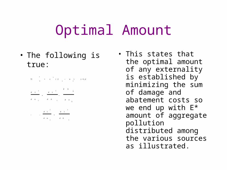
• The following is true:

• This states that the optimal amount of any externality is established by minimizing the sum of damage and abatement costs so we end up with E* amount of aggregate pollution distributed among the various sources as illustrated.

TCA

i

= ci

( Zi

– ei

) i =1,2

d ci

d ei

=

d ci

d Ai

•

∂ Ai

∂ ei

∴ –

d c

i

d ei

=

d c

i

d Ai

Internalizing the Externality

• If a profit maximizing firm were faced with an abatement charge they would internalize the externality or abate until the mc of abatement were equal to the price of pollution or the change; that is,

πi

= R ( Q ) – c ( Q ) c (' Ai) – c e

i

∴ set

∂ c

i

∂ Ai

= c

Government Standards

• If the government wanted to establish a 'standard' it would be . To determine these standards would require knowledge of:– level of marginal damages– mc function of polluters

• It would therefore appear that there is an informational advantage to pricing.

• The solution which has been illustrated above also applies with:

• 1. spatially differentiated damages• 2. non-linear damage functions• 3. non-competitive market settings

Why Standards Dominate Charges

• (A) Uncertainty with respect to the marginal damage function.

• (B) Uncertainty with respect to the marginal abatement costs.

Uncertainty with respect to the marginal damage

function• Now consider the situation

where the MC of abatement has been underestimated so the true MC of abatement lies above the estimated MC of abatement function. Consider a standards scheme. Using the estimated MC of abatement the emission level is set at e instead of e*. Thus, the emission level is too low relative to the optimum. With the level of abatement too high, the damages reduced due to having this lower level of emissions is eAce* but at the cost of much higher abatement costs of eBCe*. The net social loss will be ABC.

$/e

0

e

MC

A

T

MD

T

e

MD

eA

C

B

EC*

EC

e* e

Alternatively, suppose the authority set a sub-optimal emission standard of e because it is using the erroneous MD function. With emissions at e rather than e*, we again end up with a net social loss of ABC. Therefore, uncertainty with respect to the marginal damage function provides NO ADVANTAGE to either scheme; pricing or standards.

Uncertain with respect to marginal abatement costs

• Now consider the situation where the MC of abatement has been underestimated so the true MC of abatement lies above the estimated MC of abatement function. Consider a standards scheme. Using the estimated MC of abatement the emission level is set at e instead of e*. Thus, the emission level is too low relative to the optimum. With the level of abatement too high, the damages reduced due to having this lower level of emissions is eAce* but at the cost of much higher abatement costs of eBCe*. The net social loss will be ABC

$/e

0

e

MC

A

T

MD

T

e

A

C

B

EC*

EC

e*e

MC

A

e'

D

E• •

•

•

•

Abatement: Pricing v. Standards

• Now consider a pricing scheme. The authority would set the emission charge at EC by setting the MD function equal to the MC of abatement function. This would result in a level of emission of e; thinking this is the correct amount. But with a true MC of abatement at MCT the level of emissions which the charge EC will generate will be e'.

• e' > e* so we have too high a level of emissions. Pollution damages will increase by the amount e*CDe' but the abatement costs will be reduced (because of higher allowed emissions) by e*CEe'. Therefore, the net social loss will be CDE.

• Generally, there is no reason to expect CDE = ABC but it has been shown that

WL

T= WL

q= –

1

2

EC

e• Δ e

2 1

εD

+

1

εc

where

WLT

is the welfare loss from pricing

WLq

welfare loss from standards

Δ e is e '– e

εD

is the elasticity of the marginal damage function

εc

is the elasticity of the marginal cost of abatement function

The welfare loss from pricing and standards will be equal if 1. = in absolute valueor2. ∆e = 0 or MCA = MCT

Standards will be preferred to charges when WLT - WLq > 0, which occurs when |eD| < |eC|. If |eC| 0 charges are preferred while if || 0 standards are preferred.

Rationale

• The rationale for this is:

• (a) if the MD function is steep (e.g. with very toxic pollution) even a slight error in e will generate large damages. With uncertainty about costs, the chances of such errors is greater with a charging scheme.

• (b) if the MD function is flat, a charge will better approximate marginal damages. If the damage function is linear, the optimal result is independent of any knowledge about costs.

• (c) if the MC is steep, an ambitious standard could result in excessive costs to abators. A charge places an upper limit on costs.

• Therefore, the KEY in this is charges set an upper limit on costs while standards set an upper limit on discharges.

Externalities in Transport• Transportation sources in North America contribute

approximately

• 47% of NOx

• 71% of CO • 39% of HC

• To control most pollutants we have opted for standards rather than pricing. This is reflected in the 'level of allowed emissions' with catalytic converters on our vehicles.

• Noise is another example where the U.S. has opted for a technological fix to achieve a standard. Europeans have, however, introduced noise charges at some airports for aircraft which exceed a particular noise level.

External Prices

• Externality prices can take three forms:• 1. use to optimize social surplus• 2. use to achieve a predetermined standard

at least cost]• 3. use to induce compliance to a particular

standard• Perhaps the best know 'cure' for the

congestion externality facing most major cities has been advocated by economists; road pricing. Standards are achieved in this instance by continuing to build roads.