NBER WORKING PAPER SERIES

NEOCLASSICAL FACTORS

Long ChenLu Zhang

Working Paper 13282http://www.nber.org/papers/w13282

NATIONAL BUREAU OF ECONOMIC RESEARCH1050 Massachusetts Avenue

Cambridge, MA 02138July 2007

For helpful discussions, we thank Sreedhar Bharath, Gerald Garvey (BGI discussant), Tyler Shumway,Motohiro Yogo (UBC discussant), Richard Sloan, Scott Richardson, and seminar participants at BarclaysGlobal Investors, Hong Kong University of Science and Technology, UBC PH&N Summer FinanceConference in 2007, and University of Michigan. Cynthia Jin provided valuable assistance in earlystages of this project. The views expressed herein are those of the author(s) and do not necessarilyreflect the views of the National Bureau of Economic Research.

© 2007 by Long Chen and Lu Zhang. All rights reserved. Short sections of text, not to exceed twoparagraphs, may be quoted without explicit permission provided that full credit, including © notice,is given to the source.

Neoclassical FactorsLong Chen and Lu ZhangNBER Working Paper No. 13282July 2007JEL No. G11,G12,G14,G24,G31,G32

ABSTRACT

Building on neoclassical reasoning, we propose a new multi-factor model that consists of the marketfactor and factor mimicking portfolios based on investment and productivity. The neo- classical three-factormodel outperforms traditional factor models in explaining the average returns across testing portfoliosformed on momentum, financial distress, investment, profitability, accruals, net stock issues, earningssurprises, and asset growth. Most intriguingly, winners have higher loadings than losers on both thelow-minus-high investment factor and the high- minus-low productivity factor, which in turn helpexplain momentum profits.

Long Chen321 EppleyDepartment of FinanceThe Eli Broad Graduate School of ManagementMichigan State UniversityEast LansingMI 48824chen@bus.msu.edu

Lu ZhangFinance DepartmentStephen M. Ross School of BusinessUniversity of Michigan701 Tappan Street, ER 7605 Bus AdAnn Arbor MI, 48109-1234and NBERzhanglu@bus.umich.edu

1 Introduction

The Sharpe (1964) and Lintner (1965) capital asset pricing model (CAPM) cannot explain many

anomalies. For example, DeBondt and Thaler (1985), Fama and French (1992), and Lakonishok,

Shleifer, and Vishny (1994) show that average returns covary with book-to-market, earnings-to-

price, and long-term prior returns. Jegadeesh and Titman (1993) show that stocks with higher

short-term prior returns earn higher average returns. Fama and French (1993, 1996) show that

their three-factor model, which includes the market excess return (MKT ), a mimicking portfolio

based on market equity (SMB), and a mimicking portfolio based on book-to-market (HML), can

explain many CAPM anomalies. These include average returns across portfolios formed on size and

book-to-market, earnings-to-price, cash flow-to-price, and long-term prior returns. Notably, these

portfolios display strong HML-loading variations in the same direction as their average returns.

However, the influential Fama-French (1993) three-factor model leaves important anomalies

unexplained. Most glaringly, Fama and French (1996) show that their model cannot explain Je-

gadeesh and Titman’s (1993) momentum profits. Winners load positively on HML and losers load

negatively on HML. This pattern goes in the opposite direction as the average returns, leading

the Fama-French model to exacerbate the momentum anomaly.

The relation between financial distress and average returns also eludes the Fama-French (1993)

model. Fama and French (1996) conjecture that the average HML return might be a risk premium

for the relative distress of value firms. The returns of distressed firms tend to move together, mean-

ing that their distress risk cannot be diversified and needs to be compensated with a risk premium.

However, recent studies show that the distress risk is associated with lower average returns (e.g.,

Dichev 1998, Griffin and Lemmon 2002, Campbell, Hilscher, and Szilagyi 2007). Using a compre-

hensive measure of financial distress, Campbell et al. report that more distressed stocks earn lower

average returns despite their higher total volatilities, market betas, and SMB- and HML-loadings.1

We show that the momentum and the distress anomalies are related, and are captured by a new

multi-factor model motivated from neoclassical reasoning. The model says that the expected return

on a portfolio in excess of the risk-free rate, E[Rj ]−Rf , is described by the sensitivity of its return

to three factors: MKT , the difference between the return on a portfolio of low investment-to-assets

stocks and the return on a portfolio of high investment-to-assets stocks (INV ), and the difference

1Campbell, Hilscher, and Szilagyi (2007) conclude that: “This result is a significant challenge to the conjecture thatthe value and size effects are proxies for a financial distress premium. More generally, it is a challenge to standard mod-els of rational asset pricing in which the structure of the economy is stable and well understood by investors (p. 29).”

2

between the return on a portfolio of high earnings-to-assets stocks and the return on a portfolio of

low earnings-to-assets stocks (PROD). Specifically, the expected excess return on portfolio j is:

E[Rj ] − Rf = bj E[MKT ] + ij E[INV ] + pj E[PROD] (1)

in which E[MKT ], E[INV ], and E[PROD] are expected premiums, and the factor loadings, bj , ij ,

and pj are the slopes in the time series regression:

Rj − Rf = aj + bj MKT + ij INV + pj PROD + εj (2)

In our 1972–2006 sample, INV and PROD earn average returns of 0.34% (t = 4.15) and 0.73%

per month (t = 5.67), respectively. These average returns subsist after adjusting for their expo-

sures to traditional factors such as the Fama-French (1993) factors and the Carhart (1997) factors.

We find that the neoclassical three-factor model goes a long way in describing the cross section of

average returns on NYSE, Amex, and NASDAQ stocks.

Most important, the neoclassical model outperforms the Fama-French (1993) model in explain-

ing the average returns of 25 size and momentum portfolios. Using the six-month momentum

definition of Jegadeesh and Titman (1993), we find that none of the winner-minus-loser portfolios

across five size quintiles have significant alphas. The alphas, ranging from −0.02% to 0.34% per

month, are all within 1.6 standard errors of zero. For comparison, the five winner-minus-loser

alphas vary from 0.64% (t = 2.77) to 1.02% per month (t = 6.04) in the CAPM and from 0.75%

(t = 2.92) to 1.14% per month (t = 6.07) in the Fama-French model. In total, seven out of the

25 size and momentum portfolios have significant neoclassical alphas, and our model is rejected by

the Gibbons, Ross, and Shanken (1989, GRS) test. However, the number of significant alphas is

about half of that in the CAPM (13) and that in the Fama-French model (13).

One reason for the relative success of the neoclassical model is that winners have higher PROD-

loadings than losers, meaning that winners are more profitable than losers. More intriguingly, win-

ners also have higher INV -loadings than losers. The crux is timing. We show that winners (with

high valuation ratios) indeed invest more than losers (with low valuation ratios) at the portfolio

formation month t. But more important, winners invest less than losers in the event time before

month t−8 or t−12, depending on the specific size quintile. Because INV is rebalanced annually,

the higher INV -loadings for winners accurately reflect their lower investment than losers several

quarters prior to the monthly portfolio formation.

3

The neoclassical model fully captures the negative relation between financial distress and aver-

age returns. The high-minus-low distress decile earns a neoclassical alpha of 0.18% per month (t =

0.83). And the model cannot be rejected using distress deciles by the GRS test (p-value = 0.08).

In contrast, the corresponding alpha is −1.23% (t = −4.15) in the CAPM and −1.34% (t = −5.22)

in the Fama-French (1993) model. And both models are rejected by the GRS test at the 1% level.

The PROD-loading is the main driver of our model performance: More distressed firms are less

profitable and have lower PROD-loadings than less distressed firms. Previous studies overlook the

productivity-return relation, and, not surprisingly, find the distress-return relation anomalous.

Since Fama and French (1996), several other anomaly variables have received much attention,

including earnings surprises, investment, profitability, accruals, net stock issues, and asset growth.

(We provide detailed references later in this section and in Section 2.) We show that the neoclassi-

cal model outperforms traditional factor models in explaining these anomalies, sometimes by a big

margin. For example, in the universe of 25 investment and profitability portfolios, the neoclassical

alphas for the five high-minus-low investment portfolios are all within 1.5 standard errors of zero.

The alpha with the highest magnitude is −0.30% per month (t = −1.45) in the lowest-profitability

quintile. In contrast, the corresponding alpha is −1.01% (t = −4.67) in the CAPM and −0.70%

(t = −3.45) in the Fama-French model. Further, the high-minus-low profitability portfolio in the

highest-investment quintile earns a neoclassical alpha of 0.27% (t = 1.34), whereas the correspond-

ing alpha is 1.22% (t = 4.96) in the CAPM and 1.43% (t = 6.08) in the Fama-French model.

However, our neoclassical model underperforms the Fama-French (1993) model in explaining

the anomalies formed on valuation ratios such as book-to-market (B/M). While the Fama-French

model explains these anomalies through their HML factor, the main driver in our model is the INV

factor. Stocks with higher valuation ratios invest less, load more on the low-minus-high INV factor,

and earn higher average returns. But empirically, the explanatory power of INV for valuation-

sorted portfolio returns is not as high as that of HML. This evidence lends support to Fama

and French (2007), who show that including net stock issues and asset growth in cross-sectional

regressions has little impact on the book-to-market effect. However, the small-growth portfolio only

earns a tiny neoclassical alpha of −0.03% per month (t = −0.10) in contrast to the CAPM alpha

of −0.63% (t = −2.61) and the Fama-French alpha of −0.52% (t = −4.48). We show that the tiny

neoclassical alpha is linked to the abysmally low profitability of the small-growth firms in the 1990s.

At a minimum, our evidence shows that the neoclassical three-factor model provides a rea-

4

sonable description of the cross section of average stock returns. This evidence, coupled with the

motivation of our factors from equilibrium asset pricing theory, suggests that the neoclassical model

can be used in many applications that require estimates of expected stock returns. The list includes

evaluating mutual fund performance, measuring abnormal returns in event studies, and estimating

expected returns for portfolio choice and costs of capital for capital budgeting.

Our work adds to a large finance and accounting literature that studies how investment and

profitability relate to average returns. Fairfield, Whisenant, and Yohn (2003), Richardson and

Sloan (2003), Titman, Wei, and Xie (2004), Anderson and Garcia-Feijoo (2006), Fama and French

(2006, 2007), Cooper, Gulen, and Schill (2007), Polk and Sapienza (2007), Lyandres, Sun, and

Zhang (2007), and Xing (2007) show that firms that invest more earn lower average returns. Ball

and Brown (1968), Bernard and Thomas (1989, 1990), Ball, Kothari, and Watts (1993), and Chan,

Jagadeesh, and Lakonishok (1996) show that firms with higher earnings surprises earn higher av-

erage returns. Haugen and Baker (1996), Abarbanell and Bushee (1998), Frankel and Lee (1998),

Dechow, Hutton, and Sloan (1999), Piotroski (2000), Cohen, Gompers, and Vuolteenaho (2002),

and Fama and French (2006, 2007) show that more profitable firms earn higher average returns.

Our work adds to the literature in two ways. First, we show that the combined effect of prof-

itability and, more surprisingly, investment, substantially reduces abnormal momentum profits. We

also show that the distress anomaly simply reflects the positive earnings-return relation. Second, we

complement Fama and French’s (2006) effort in providing a unifying perspective for many anoma-

lies that are often treated in isolation. While Fama and French derive their testable predictions

from valuation theory, we derive our hypotheses from neoclassical investment theory. To the extent

that there is no over- or under-reaction in our theory, we reinforce Fama and French’s conclusion

that, despite common claims to the contrary, empirical tests in the anomalies literature cannot by

themselves tell us whether the anomalies are driven by rational or irrational forces. In fact, our

theory and tests suggest that the anomalies can be consistent with Efficient Market Hypothesis.

Our story proceeds as follows. Section 2 motivates our neoclassical factors and discusses our

empirical strategy. Section 3 uses time series tests to show that the neoclassical model helps explain

anomalies. Section 4 reports cross-sectional tests. We conclude in Section 5.

2 Economic Hypotheses and Empirical Strategy

Section 2.1 develops testable hypotheses, and Section 2.2 discusses our empirical strategy.

5

2.1 Testable Hypotheses

We start from the q-theoretical framework a la Cochrane (1991, 1996). Within this framework, we

derive a characteristics-based expected-return equation (see equation A.8 in Appendix A) — the

two-period simplification of the infinite-horizon equation in Liu, Whited, and Zhang (2007):

Expected return =Expected profitability + 1

Marginal cost of investment(3)

Thus, the q-theory in its simplest form says that the expected return is the expected profitability

divided by marginal cost of investment (which increases with investment). Equation (3) sheds

light on anomalies because expected returns are directly tied with firm characteristics. Specifically,

investment and expected profitability emerge as the two central drivers of expected returns.

2.1.1 The Investment Hypothesis

Equation (3) says that expected returns decrease with investment-to-assets, given expected prof-

itability. The intuition is perhaps most transparent in the capital budgeting language of Brealey,

Myers, and Allen (2006). Given expected cash flows, higher costs of capital imply lower net present

values of new capital, which in turn mean lower investment-to-assets. More important, investment is

the common driver of many anomalies, including value, net stock issues, accruals, and asset growth:

The Investment Hypothesis: The negative investment-return relation drives the positive

relations of average returns with book-to-market and earnings-to-price as well as the

negative relations of average returns with accruals, net stock issues, and asset growth.

2.1.1.1 Intuition The q-theory gives rise to a direct link between book-to-market and investment-

to-assets. Optimal investment implies that investment-to-assets is an increasing function of marginal

q, which is closely related to average q or market-to-book.2 Reflecting the negative investment-

return relation, value firms earn higher average returns than growth firms. Other valuation ratios

such as earnings-to-price also can capture cross-sectional differences in investment opportunity set,

and are connected to investment policies. In general, firms with higher valuation ratios have more

growth opportunities, invest more, and earn lower expected returns.

The negative investment-return relation also manifests itself as the net stock issues anomaly,

2More precisely, the marginal q equals the average q under constant returns to scale, as shown in Hayashi (1982)and Abel and Eberly (1994). But the average q and market-to-book equity are closely correlated, and are identicalin models with all equity financing. See Liu, Whited, and Zhang (2007) for detailed derivations.

6

the accrual anomaly, and the asset growth anomaly. Ritter (1991), Loughran and Ritter (1995),

and Spiess and Affleck-Graves (1995) show that equity issuers underperform matching nonissuers

in post-issue years. Ikenberry, Lakonishok, and Vermaelen (1995) show that firms conducting open

market share repurchases outperform matching firms in post-event years. Pulling together the

earlier evidence, Daniel and Titman (2006) and Pontiff and Woodgate (2006) report a negative

relation between net stock issues and average returns. Fama and French (2007) show that the net

stock issues effect is pervasive and shows up in all size groups.

The net issues anomaly is often interpreted as investors underreacting to managerial market

timing. But Lyandres, Sun, and Zhang (2007) argue that the balance-sheet constraint of firms

requires that the uses of funds must equal the sources of funds, meaning that issuers should in-

vest more and earn lower average returns than nonissuers. Lyandres et al. show that adding an

investment factor into the CAPM and the Fama-French (1993) model substantially reduces the

magnitude of the underperformance following initial public offerings, seasoned equity offerings, and

convertible debt offerings. We add to their work in two ways: We follow Fama and French (2007)

in using a more comprehensive net issues measure that takes into account share repurchases. And

besides INV , we also study the role of PROD in driving the net issues anomaly.

Sloan (1996) shows that firms with high accruals earn abnormally low average returns than firms

with low accruals (see also Xie 2001; Fairfield, Whisenant, and Yohn 2003; Richardson, Sloan, Soli-

man, and Tuna 2004; Hirshleifer, Hou, Teoh, and Zhang 2004). Sloan interprets the evidence as

investors overestimating the persistence of the accrual component of earnings only to be systemat-

ically surprised later on. But interpreting accruals as working capital investment, Wu, Zhang, and

Zhang (2007) hypothesize that firms rationally adjust their working capital investment to respond

to discount rate changes. Wu et al. show that adding the investment factor into the CAPM and

the Fama-French (1993) model substantially reduces the magnitude of the accrual anomaly. We

complement their work by using the accruals measure from Fama and French (2007) that adjusts

for the effect of changes in the scale of firms caused by share issues and repurchases. We verify

that investment is important in driving the accrual anomaly, but productivity is not.

Cooper, Gulen, and Schill (2007) show that asset growth, defined as the annual changes in total

assets divided by lagged total assets, strongly predicts future returns with a negative sign. Follow-

ing Titman, Wei, and Xie (2004), Cooper et al. interprets the evidence as investors underreacting

to managerial overinvestment. Our view is that asset growth is arguably the most comprehensive

7

measure of investment-to-assets, in which investment is simply the changes in total assets.

2.1.1.2 Discussion Noteworthy, the negative investment-return relation is conditional on ex-

pected profitability. This point is important because expected profitability is not disconnected from

investment-to-assets: More profitable firms invest more both in the data (e.g., Fama and French

1995) and in theory (e.g., Zhang 2005). The conditional nature of the investment-return relation of-

fers the following portfolio interpretation of the investment hypothesis. Sorting on book-to-market,

earnings-to-price, accruals, net stock issues, and asset growth is closer to sorting on investment-to-

assets than sorting on expected profitability. These sorts tend to generate higher magnitudes of

spread in investment-to-assets than in expected profitability. Thus, we can interpret the average

return variations generated from these diverse sorts using their common implied sort on investment.

2.1.2 The Productivity Hypothesis

Complementing the investment hypothesis, equation (3) also says that given investment-to-assets,

firms with higher expected profitability should earn higher expected returns.

The Productivity Hypothesis: The positive profitability-return relation drives the posi-

tive relations of average returns with earnings surprises and short-term prior returns as

well as the negative relation between average returns and financial distress.

2.1.2.1 Intuition As noted, marginal cost of investment equals marginal q, which is basically

average q or market-to-book. Equation (3) then says that the expected return equals the expected

profitability divided by market-to-book. The intuition is exactly analogous to that from the Gordon

(1962) Growth Model. Imagine a two-period version of that model: Price equals expected cash flow

divided by the discount rate. So high expected cash flow (or expected profitability) relative to low

price (or market valuation ratios) means high discount rates. And to the extent that there is no

over- or under-reaction (all the expectations are rational) in our neoclassical model, high discount

rates correspond to high risk (see equation A.10 for the formal link between risk and characteristics).

Going beyond the discounting intuition from valuation theory, our investment-based theory

provides additional capital budgeting intuition for the positive productivity-return relation. Recall

the original formulation of equation (3) says that the expected return is the expected profitability

divided by an increasing function of investment-to-assets. So high expected profitability relative

to low investment must mean high discount rates: Otherwise firms would observe high net present

8

values of new capital and invest more. Conversely, low expected profitability relative to high in-

vestment (such as the small-growth firms in the 1990s) must mean low discount rates: Otherwise

these firms would observe low net present values of new capital and invest less.

The positive productivity-return relation has important portfolio implications. For any sorts

that generate higher magnitudes of spread in expected profitability than in investment-to-assets,

their average return patterns can be explained using the productivity hypothesis. We explore three

such sorts, sorts on earnings surprises, on short-term prior returns, and on financial distress.

Sorting on earnings surprises can generate a profitability spread between extreme portfolios.

The intuition is that firms that have experienced large, positive earnings surprises are more prof-

itable than firms that have experienced large, negative earnings surprises. Sorting on momentum

also should generate an important spread in profitability.3 The intuition is that shocks to earn-

ings are positively correlated with shocks to stock returns contemporaneously. Firms that just

beat earnings expectations are likely to experience stock price increases, whereas firms that fall

below earnings expectations are likely to experience stock price decreases. The distress anomaly

of Campbell, Hilscher, and Szilagyi (2007) can be another reflection of the positive productivity-

return relation. The intuition is that less distressed firms are more profitable and should earn higher

average returns, even though they are less levered. And more distressed firms are less profitable

and should earn lower average returns, even though they are more levered.

2.2 Empirical Strategy: Strengths and Weaknesses

We primarily use the Fama-French (1993) portfolio approach to explore our economic hypotheses.

We are attracted to the portfolio approach because of its powerful simplicity. The widespread use of

this approach also allows us to easily compare our empirical results to those from the prior literature.

2.2.1 From Theory to Practice

We construct factor mimicking portfolios based on investment-to-assets and earnings-to-assets,

which, according to equation (3), are pivotal economic determinants of expected returns. Because

these two factors are derived from the partial equilibrium q-theory that studies the optimal invest-

ment of firms, we also include the market factor, MKT , which can be derived from the partial

equilibrium theory of consumption (see, for example, Cochrane 2005, p. 155–156). The resulting

3Liu and Zhang (2007) show that winners have temporarily higher expected profitability and expected growth ratesthan losers. The duration of the expected-growth spread also matches roughly the duration of momentum profits.

9

three-factor specification (MKT + INV + PROD), dubbed the neoclassical three-factor model,

can be interpreted as the portfolio implementation of the Arrow-Debreu general equilibrium theory.

We use the neoclassical three-factor model as a parsimonious and practical model for estimating

expected returns. In the same way that Fama and French (1996) test their three-factor model, we

regress excess returns of a wide range of testing portfolios on the neoclassical factor returns as in

equation (2). If the neoclassical model adequately describes the cross section of average returns,

the intercepts should be statistically indistinguishable from zero.

The portfolio approach differs from alternative methods that have been used to explore the em-

pirical foundation of investment-based asset pricing. Zhang (2005), Cooper (2006), and Gala (2006)

build full-fledged equilibrium models and examine if model-implied moments match key facts in the

data. This quantitative theory approach a la Kydland and Prescott (1982) is useful to understand

underlying economic mechanisms, but it does not provide an easy-to-use model for calculating

expected returns in practice. Liu, Whited, and Zhang (2007) parameterize the production and

investment technologies of firms in the right-hand-side of equation (3), and use GMM to minimize

the average differences between both sides of the equation. This structural estimation approach

a la Hansen and Singleton (1982) is closely linked to the underlying theory, and it also provides

an empirical expected-return model. But the model is more complicated to implement than most

models in empirical finance. Our portfolio approach can be viewed as a linearized implementation

of Liu et al.’s nonlinear estimation. As noted, although the link between theory and tests is not as

close, we adore the portfolio approach because of its powerful simplicity.

We also supplement time series tests on sorted portfolios with Fama and MacBeth (1973) cross-

sectional regressions on characteristics. We do so for several reasons. First, our empirical analysis

builds on prior studies that use variables such as investment and profitability in cross-sectional

tests (e.g., Fama and French 2006, 2007). Replicating their tests with our sample and variable

definitions is useful for comparison. Second, more important, we motivate INV and PROD from

the q-theory, which directly ties expected returns to investment and profitability characteristics.

Thus, using characteristics in cross-sectional regressions can be a more direct test of the theory.

Third, cross-sectional regressions can be more powerful that time series tests in some circumstances

because they provide an easier way to control for all the characteristics simultaneously.

While sensitive to the differences between time series and cross-sectional tests (see, e.g., Fama

and French 2007, p. 2–3), we view these two methods as closely related. If a variable shows up signif-

10

icantly in cross-sectional tests, its factor mimicking portfolio is likely to have important explanatory

power in time series tests. We find time series tests easy to interpret because they provide a simple

measure of abnormal returns as the regression intercept. Fortunately, although our test results

from the two approaches sometimes differ in nuances, they provide the same general inferences.

2.2.2 Interpreting Neoclassical Factors

Following Fama and French (1993, 1996), we interpret our neoclassical factors as common factors

in the cross section of returns. While Fama and French pursue a more aggressive interpretation

that their similarly constructed SMB and HML are risk factors in the context of ICAPM or APT,

we shy away from taking a strong stance on the risk interpretation of our factors.

On the one hand, the theoretical arguments we use to motivate the two factors are based on

recent developments in equilibrium asset pricing theory, which does not allow any form of mispric-

ing. The crux is that, just like consumption-based asset pricing predicts that aggregate expected

returns covary with business cycles, investment-based asset pricing predicts that expected returns

in the cross section covary with firm characteristics, corporate policies, and events. The latter set of

endogenous relations cannot possibly be captured by consumption-based frameworks because char-

acteristics are not even modeled. Thus, rejecting the CAPM (a canonical consumption-based model)

does not mean rejecting Efficient Market Hypothesis because of the bad-model problem (e.g., Fama

1998). And perhaps because of the lack of readily available measures, behavioralists often use valu-

ation ratios to proxy for mispricing. Interpreting Fama and French’s (1993) factors is controversial

because size and B/M directly involve market equity. But our neoclassical factors are constructed

on economic fundamentals that are less likely to be affected by mispricing, at least directly.

On the other hand, Polk and Sapienza (2006) show that investor sentiment can affect investment

and hence future profitability through shareholder discount rates. Managerial overconfidence also

can distort corporate investment because hubristic managers tend to overestimate the returns to

their pet projects (e.g., Malmendier and Tate 2005). Our tests cannot rule out these interpretations.

More important, risk-based and characteristics-based interpretations on any common factor are

not mutually exclusive: In fact, they are the two sides of the same coin. Challenging the Fama

and French (1993) risk interpretation of their SMB and HML factors, Daniel and Titman (1997)

argue that it is the size and B/M characteristics rather than the covariance structure of returns

that explain the cross section of average returns. However, emerging from investment-based asset

11

pricing is the fresh insight that characteristics are sufficient statistics of expected returns: The

right-hand-side of equation (3) only involves characteristics. Further, an analytical link exists

between covariances and characteristics (see equation A.10 in Appendix A), meaning that covari-

ances and characteristics are equivalent predictors of returns, at least in theory. But in practice,

characteristics-based models are likely to dominate covariances-based models. The reason is simple:

In a time-varying, dynamic world, characteristics are more precisely measured than covariances.

And a horse race often declares characteristics as the winner. This is the case even in simulated

data generated from dynamic single-factor models (e.g., Gomes, Kogan, and Zhang 2003). Thus,

it is conceivable that the relative success of characteristics-based models in asset pricing tests is

driven by measurement errors in betas rather than systematic mispricing. After all, neoclassical

investment theory predicts that characteristics should covary with expected returns to begin with.

3 Time Series Regressions

We report our main results from time series tests. We first construct the explanatory factors in Sec-

tion 3.1. We then use the neoclassical three-factor model to explain average returns for a wide range

of testing portfolios, including both two-way sorted (Section 3.2) and one-way sorted (Section 3.3).

3.1 The Explanatory Factors

This subsection constructs and reports the properties of the investment and productivity factors.

3.1.1 The Investment Factor, INV

Following the Fama and French (1993) portfolio approach, we construct INV from a double (two

by three) sort on size and investment-to-assets. (Appendix B describes our sample construction

and variable definitions in details.) In June of each year t, all NYSE stocks on CRSP are sorted on

market equity (stock price times shares outstanding). We use the median NYSE size to split NYSE,

Amex, and NASDAQ stocks into two groups. We also break NYSE, Amex, and NASDAQ stocks

into three investment-to-assets (I/A) groups based on the breakpoints for the low 30%, middle

40%, and high 30% of the ranked values for stocks traded on NYSE. We use NYSE breakpoints

in constructing factors and testing portfolios throughout the paper to help ensure that none of the

portfolios are excessively dominated by micro-caps and small stocks (e.g., Fama and French 2007).

We form six portfolios from the intersections of the two size and the three I/A groups. Monthly

value-weighted returns on the six portfolios are calculated from July of year t to June of t+1, and

12

the portfolios are rebalanced in June of t+1. We calculate returns beginning in July of year t to

ensure that investment for year t−1 is known. The INV factor is designed to mimic the common

variations in returns related to investment-to-assets: INV is the difference (low-minus-high invest-

ment), each month, between the simple average of the returns on the two low-I/A portfolios and

the simple average of the returns on the two high-I/A portfolios.

From Table 1, the average INV return in our sample is 0.34% per month (t = 4.15). Regressing

INV on MKT generates an alpha of 0.41% per month (t = 5.54) and a R2 of 17%. Regressing

INV on the Fama and French (1993) model and the Carhart (1997) model reduces the alpha to

0.26% and 0.17% per month (t = 3.66 and 2.39), and increases the R2 to 31% and 35%, respectively.

(The data for the Fama-French factors and the momentum factor are from Kenneth French’s Web

site.) Thus, INV captures average return variations not subsumed by the other common factors.

INV has a relatively high correlation of 0.51 with HML (p-value = 0). This evidence is con-

sistent with Xing (2006), who shows that an investment growth factor contains information similar

to HML and can explain the value effect roughly as well as HML. Xing constructs her factor

by sorting on the growth rate of capital expenditure. The average return of her factor is only

0.20% per month, albeit significant. We follow Lyandres, Sun, and Zhang (2007) in using a more

comprehensive measure of investment that includes both long-term and short-term investments.

As a result, our investment factor earns a higher average return.

Panel C of Table 1 provides more details on the six size-I/A portfolios underlying the INV fac-

tor. Sorting on I/A generates a large spread in I/A: Portfolio SLI (small-size and low-investment)

has an average I/A of −3.44% per annum, whereas portfolio SHI (small-size and high-investment)

has an average of 28%. Portfolio SHI is also more profitable than portfolio SLI : The earnings-to-

assets (ROA) of portfolio SHI is 1.17% per quarter versus 0.66% for portfolio SLI . Portfolio SLI

also has a higher average prior 2–12 month return (from July of year t−1 to May of year t) than port-

folio SHI , 22% versus 15%. This evidence partially reflects the fact that low-investment firms have

higher average future returns than high-investment firms. (We follow Fama and French (1993) in

sorting stocks in June on accounting information at the last fiscal year-end to guard against the look-

ahead bias.) The evidence does not mean that low-investment firms have higher average contem-

poraneous returns. In untabulated results, we measure returns over the calendar year t−1 and find

that portfolio SLI has lower average contemporaneous returns than portfolio SHI , 18% versus 27%.

13

3.1.2 The Productivity Factor, PROD

We construct PROD based on earnings-to-assets, ROA. Using cash-flow-to-assets to measure pro-

ductivity does not materially affect our results (not reported). We sort on current profitability, as

opposed to expected profitability. The reason is that profitability is highly persistent (e.g., Fama

and French 1995, 2000, 2006). In particular, Fama and French (2006) show that current profitabil-

ity is the strongest predictor of future profitability, meaning that current profitability is highly

correlated with the expected profitability, to which equation (3) applies.

Because PROD is most relevant for explaining momentum profits that are constructed monthly,

we use a similar approach to construct PROD. In particular, we use quarterly data to measure

ROA. Indeed, using annual sorts on annual earnings-to-assets at the last fiscal year-end yields an

insignificant average return of only five basis points per annum for the productivity factor. This

evidence is consistent with that reported by Fama and French (2007, Table II).

However, we also find that the original earnings and momentum anomalies do not survive the

frequency change from monthly to annual rebalancing either. Specifically, in June of each year t,

we sort all NYSE, Amex, and NASDAQ stocks into ten deciles based on the NYSE breakpoints of

the Standardized Unexpected Earnings (SUE) measured at the fiscal year-end of t−1, the average

SUE over the last fiscal year, the annual return over the calendar year t−1, and the 12-month

return from June of year t−1 to May of year t. Monthly value-weighted returns of these portfolios

are calculated from July of year t to June of year t+1. Untabulated results show that none of these

strategies generate mean excess returns or CAPM alphas that are significantly different from zero.

Because the SUE and momentum anomalies only exist in monthly rebalancing, it seems reasonable

to construct the explanatory PROD factor in the same frequency.

Nevertheless, we emphasize that using quarterly earnings to construct PROD, while using an-

nual investment to construct INV , is largely driven by data, not by theory. The growing literature

on investment-based asset pricing does predict that earnings and prior returns can be related to

time-varying expected returns.4 However, to the best of our knowledge, the theoretical literature

has so far not addressed the question why earnings and momentum anomalies are more short-lived

than others such as value and investment anomalies. This caveat also applies to our work.

4See Berk, Green, and Naik (1999), Johnson (2002), and Sagi and Seasholes (2007) for recent examples that relateprior short-term returns to expected returns. Liu and Zhang (2007) document that recent winners have temporarilyhigher loadings than recent losers on the growth rate of industrial production. Liu, Whited, and Zhang (2007) showthat an investment-based expected return model can partially explain the earnings anomaly.

14

To construct PROD, each month from January 1972 to December 2006, we categorize NYSE,

Amex, and NASDAQ stocks into three groups based on the NYSE breakpoints for the low 30%,

middle 40%, and high 30% of the ranked values of quarterly ROA from at least four months ago.

The choice of the four-month lag is conservative: Using shorter lags only serves to strengthen our re-

sults (not reported). We use the four-month lag to ensure that the required accounting information

is known before we form the portfolios. We also use the NYSE median market equity each month to

split NYSE, Amex, and NASDAQ stocks into two groups. We form six portfolios from the intersec-

tions of the two size and three ROA groups. Monthly value-weighted returns on the six portfolios

are calculated for the current month, and the portfolios are rebalanced monthly. The PROD factor

is meant to mimic the common variations in returns related to firm-level productivity: PROD is the

difference (high-minus-low productivity), each month, between the simple average of the returns on

the two high-ROA portfolios and the simple average of the returns on the two low-ROA portfolios.

From Panel A of Table 1, PROD earns an average return of 0.73% per month (t = 5.67) from

January 1972 to December 2006. Regressing the PROD return on the market factor, the Fama and

French (1993) three factors, and the Carhart (1997) four factors yields large alphas of 0.76%, 0.89%,

and 0.66% per month (t = 5.84, 7.04, and 5.43), and R2s of 1%, 10%, and 22%, respectively. This

evidence means that, like INV , PROD also captures average return variations not subsumed by

well-known common factors. Panel B reports that PROD and WML have a high correlation of 0.36

(p-value = 0). Intuitively, shocks to earnings are positively correlated with contemporaneous shocks

to returns. Thus, we expect PROD to have certain explanatory power for momentum profits.

Intriguingly, the correlation between INV and PROD is only −0.06 (p-value = 0.19), meaning

no need to neutralize the two factors against each other. The low correlation is counterintuitive

because one would expect that more profitable firms should invest more and that the two factors

should be negatively correlated. The low correlation results from our use of quarterly earnings to

construct PROD but annual investment to construct INV . If we instead use annual earnings data

to construct the productivity factor, we find its correlation with INV to be −0.20 (p-value = 0).

And if we use quarterly investment data to construct the investment factor, we find its correlation

with PROD to be −0.33 (p-value = 0). Thus, matching rebalancing frequency increases the posi-

tive correlation between investment and earnings, thereby increasing the magnitude of the negative

correlation between their factor mimicking portfolio returns.

Panel D of Table 1 provides more details on the six size-ROA portfolios underlying PROD. Sort-

15

ing on ROA generates a large spread in ROA: Portfolio SLP (small-size and low-productivity) has

an average ROA of −1.78% per quarter, whereas portfolio SHP (small-size and high-productivity)

has an average ROA of 3.41%. The large ROA spread only corresponds to a modest spread in annual

I/A: 11.4% versus 12.6%. The evidence helps explain the low correlation between INV and PROD

reported earlier. And the ROA spread in small firms corresponds to a large spread in prior 2–12

month returns: 9.4% versus 34.8%, helping explain the high correlation between PROD and WML.

3.2 Tests on Two-Way Sorted Portfolios

We report time series regressions of two-way sorted testing portfolios formed on size and momen-

tum, size and book-to-market, and investment and profitability. We study momentum and value

portfolios because these are arguably most important anomalies in the cross section. We also study

investment and profitability portfolios because our factors are constructed on these characteristics.

3.2.1 Preliminaries

We start by describing the construction and the basic properties of testing portfolios.

3.2.1.1 The Size-Momentum Portfolios The 25 size-momentum portfolios are from Ken-

neth French’s Web site. Fama and French (1996) use the “11/1/1” convention to measure momen-

tum. For each month t, stocks are sorted on their prior returns from month t−2 to t−12 (skipping

month t−1), and the subsequent portfolio returns are calculated for the current month t. The 25 size

and 11/1/1-momentum portfolios are formed monthly as the intersection of five portfolios sorted on

size and five portfolios sorted on prior 2–12 month returns. The monthly breakpoints are the NYSE

market equity quintiles, and the monthly prior 2–12 month returns breakpoints are NYSE quintiles.

Following Jegadeesh and Titman (1993), we also construct an alternative set of 25 size and mo-

mentum portfolios using the “6/1/6” convention of momentum. For each month t, we use NYSE

breakpoints to sort stocks on their prior returns from month t−2 to t−7 (skipping month t−1),

and calculate the subsequent portfolio returns from month t to t+5. We also use NYSE market

equity quintiles to sort all stocks independently each month into five size portfolios. The 25 size

and 6/1/1-momentum portfolios are formed monthly as the intersection of the five size quintiles

and the five quintiles based on prior 2–7 month returns.

Table 2 reports large momentum profits, especially in small firms. Panel A uses the “11/1/1”

convention of momentum. The winner-minus-loser (W -L) average return varies from 0.64% per

16

month (t = 2.16) in the biggest-size quintile to 1.72% (t = 7.63) in the smallest-size quintile. In to-

tal, 16 out of 25 size and momentum portfolios have significant CAPM alphas. The null hypothesis

that the 25 CAPM alphas are jointly zero is strongly rejected by the GRS test: The test statis-

tic (FGRS) is 6.22 (p-value = 0). More important, the CAPM alphas for the winner-minus-loser

portfolios are significant positive across all five size quintiles. The small-stock W -L strategy, in

particular, earns a CAPM alpha of 1.78% per month (t = 8.23). Consistent with Fama and French

(1996), their three-factor model exacerbates the momentum anomaly: 18 out of 25 Fama-French

alphas are significant. And the Fama-French alphas for the W -L portfolios are all larger than their

corresponding CAPM alphas. In particular, the small-stock W -L strategy earns a Fama-French

alpha of 1.96% per month (t = 7.97). The reason is that losers have higher HML-loadings than

winners: Losers behave more like value stocks, and the Fama-French model predicts that losers

should earn higher average returns, instead of lower average returns as we see in the data.

The results from the 25 size and 6/1/6-momentum portfolios are similar, but the magnitude of

momentum profits is smaller than that with the 11/1/1-momentum. The mean excess return of the

W -L portfolio ranges from 0.64% per month (t = 2.82) in the biggest-size quintile to 0.97% (t =

5.48) in the smallest-size quintile. The CAPM fails to explain the average returns of these testing

portfolios: 13 out of 25 individual alphas are significant. And the GRS test rejects the model at the

1% level. In particular, the small-stock W -L strategy earns an alpha of 1.02% per month (t = 6.04).

The Fama-French (1993) model again generates larger pricing errors than the CAPM. The W -L

alpha from the Fama-French model ranges from 0.75% (t = 2.92) to 1.14% per month (t = 6.07).

3.2.1.2 The 25 Investment-Profitability Portfolios We sort all NYSE, Amex, and NAS-

DAQ stocks into five profitability quintiles each month based on NYSE breakpoints of quarterly

ROA from at least four months ago. Also, we sort all stocks independently in June of each year

into five quintiles based on NYSE breakpoints of investment-to-assets at the last fiscal year-end.

Taking intersections yields 25 investment and profitability portfolios. Their value-weighted returns

are calculated for the current month, and the portfolios are rebalanced monthly.

Panel A of Table 3 reports descriptive statistics for the 25 investment-profitability portfolios.

High ROA stocks earn higher average returns than low ROA stocks, especially among high invest-

ment firms. And high investment stocks earn lower average returns than low investment stocks,

especially among low ROA firms. The average high-minus-low ROA portfolio return varies from

0.40% per month (t = 1.64) in the lowest-I/A quintile to 1.17% (t = 4.81) in the highest-I/A quin-

17

tile. The average low-minus-high I/A portfolio return varies from an insignificant 0.16% per month

in the highest-ROA quintile to 0.93% (t = 4.30) in the lowest-ROA quintile. The null hypothesis

that all the CAPM alphas are jointly zero is rejected at the 1% level. Despite their higher average

returns, high ROA firms have lower SMB and HML loadings than low ROA firms. Consequently,

12 out of 25 portfolios have significant alphas in the Fama-French (1993) model, in contrast to only

five significant alphas out of 25 in the CAPM.

3.2.1.3 The 25 Size-B/M Portfolios We obtain the 25 Size-B/M portfolios from Kenneth

French’s Web site. These portfolios are the intersections of five size portfolios and five B/M portfo-

lios at the end of each June. The size breakpoints for year t are the NYSE market equity quintiles

at the end of June of t. B/M for year t is the book equity for the last fiscal year-end in t−1 divided

by market equity for December of t−1. The B/M breakpoints are also NYSE quintiles.

Confirming many previous studies, Panel B of Table 3 shows that value stocks earn higher

average returns than growth stocks. The average high-minus-low (H-L) return is 1.09% per month

(t = 5.08) in the smallest-size quintile versus 0.25% (t = 1.20) in the biggest-size quintile. The

CAPM cannot explain the value premium: 15 out of 25 portfolios have significant alphas and the

GRS statistic is 4.25 (p-value = 0). Further, three out of five H-L strategies have significant alphas.

In particular, the small-stock H-L portfolio earns a positive alpha of 1.32% per month (t = 7.10).

The Fama and French (1993) model represents an impressive improvement over the CAPM

in capturing the average returns across the 25 size-B/M portfolios. The number of significant

alphas reduces from 15 to only six. The small-stock H-L alpha is reduced to 0.68% per month

(albeit still significant, t = 5.50), which is 48% lower than its CAPM alpha. The reason is that,

as highlighted in Fama and French (1996), their three-factor model generates systematic variations

in factor loadings: Small stocks have higher SMB loadings than big stocks, and value stocks have

higher HML loadings than growth stocks. The average R2 across the 25 portfolios is 89%, so even

small intercepts are often distinguishable from zero.

3.2.2 Neoclassical Regressions: The Size-Momentum Portfolios

The neoclassical model outperforms traditional models in pricing the size-momentum portfolios.

3.2.2.1 Benchmark Estimation Table 4 reports the neoclassical regressions of the size and

momentum portfolios. Panel A shows that the W -L 11/1/1-momentum strategy has a significant

18

alpha of 0.89% per month (t = 3.25) in the smallest size quintile and 0.61% (t = 2.36) in the second

size quintile. But the alphas are insignificant in the three other size quintiles. In contrast, the

W -L alpha is significant across all five size quintiles in both the CAPM and the Fama and French

(1993) model (see Table 2). This performance improvement is noteworthy. For example, although

still significant (t = 3.25), the small-stock W -L alpha of 0.89% per month in the neoclassical model

represents a reduction of 50% in magnitude from its CAPM alpha (1.78%) and a reduction of 55%

from its Fama-French alpha (1.96%). Further, the average magnitude of the W -L alphas in the

neoclassical model is 0.37% per month. In contrast, the magnitude is 1.21% in the CAPM and

1.38% per month in the Fama-French model. Finally, eight out of the 25 individual alphas are

significant, giving rise to an overall rejection of the neoclassical model by the GRS test at the 1%

level. However, the number of significant alphas in the neoclassical model (8) is much lower than

that in the CAPM (16) and that in the Fama-French model (18).

The results using the 6/1/6-momentum portfolios are largely similar. Although the neoclassical

model is rejected using the 25 portfolios, the number of significant alphas (7) is lower than that in the

CAPM (13) and that in the Fama-French (1993) model (13). More important, none of the five W -L

alphas in our model are significant. In particular, the small-stock W -L alpha is 0.34% per month (t

= 1.53). This neoclassical alpha represents a reduction in magnitude of 67% from the CAPM alpha

(1.02% per month, t = 6.04) and a reduction of 70% from the Fama-French alpha (1.14%, t = 6.07).

3.2.2.2 Sources of Explanatory Power for the Neoclassical Model The relative suc-

cess of the neoclassical model in explaining momentum profits derives from two sources. First,

the PROD-loadings of momentum portfolios go in the right direction in explaining their average

returns. Table 4 shows that winners have higher PROD-loadings than losers across all five size

groups. The magnitude of the loading spreads, significant in all cases, ranges from 0.64 to 0.88

in Panel A for the 11/1/1-momentum and from 0.45 to 0.61 in Panel B for the 6/1/6-momentum.

This evidence suggests that, not surprisingly, winners are more profitable than losers.

Second, remarkably, the INV -loadings also go in the right direction in explaining momentum

profits: Winners have higher INV -loadings than losers. The magnitude of the loading spreads,

again significant across all size groups, ranges from 0.68 to 0.96 for the 11/1/1-momentum and

from 0.47 to 0.71 for the 11/1/1-momentum. The INV -loading pattern is counterintuitive: We

would expect that winners with high valuation ratios should invest more and have lower loadings

on the low-minus-high INV factor than losers with low valuation ratios.

19

To understand the driving forces behind these loading patterns, we follow the event-study ap-

proach of Fama and French (1995) to examine how ROA and I/A vary across the testing portfolios.

To preview the results: Winners indeed have higher contemporaneous investment-to-assets than

losers at the portfolio formation month. But more important, winners also have lower investment-

to-assets than losers starting from two to four quarters prior to the portfolio formation. Because

INV is rebalanced annually, the higher INV -loadings for winners accurately reflect their lower

investment-to-assets several quarters prior to the portfolio formation.

Specifically, for each portfolio formation month t = January 1972 to December 2006, we cal-

culate quarterly ROAs and annual I/As for t+m,m = −60, . . . , 60. The ROA and I/A for t+m

are then averaged across portfolio formation months t. ROA is the most recent ROA relative to

portfolio formation month t. Figure 1 reports the details for the 25 size and 11/1/1-momentum

portfolios. The results for the 25 size and 6/1/6-momentum portfolios are similar (not reported).

For a given portfolio, we plot the median ROAs and I/As among the firms in the portfolio.

From Panel A of Figure 1, although winners have higher I/As at the portfolio formation month

t, winners have lower I/As than losers from month t−60 to month t−8. Consistent with this

event-time evidence, Panel B shows that winners have higher contemporaneous I/As than losers

in the calendar time in the smallest-size quintile. We define the contemporaneous I/A as the I/A

at the current fiscal year-end. For example, if the current month is March or September 2003, the

contemporaneous I/A is the I/A at the fiscal year-end of 2003. More important, Panel C shows

further that winners also have lower lagged or sorting-effective I/As than losers in the smallest-size

quintile. We define the sorting-effective I/A as the I/A on which an annual sort on I/A in each

June (as in our construction of INV ) is based. For example, if the current month is March 2003, the

sorting-effective I/A is the I/A at the fiscal year-end of 2001 because the annual sort on I/A is in

June 2002. If the current month is September 2003, the sorting-effective I/A is the I/A at the fiscal

year-end of 2002 because the applicable sort on I/A is in June 2003. Because INV is rebalanced

annually, the lower sorting-effective I/As of winners explain their higher INV -loadings than losers.

As expected, Figure 1 also shows that winners have higher ROAs than losers for about five

quarters before and 20 quarters after the portfolio formation month (Panel D). In the calendar time,

winners have consistently higher ROAs than losers, especially in smallest-size quintile (Panels E

and F). This evidence explains the higher PROD-loadings for the winners documented in Table 4.

20

3.2.2.3 Quarterly Investment Factor To verify that the annual rebalancing of INV is in-

deed the driving force of the INV -loading pattern across momentum portfolios, we experiment

with an alternative investment factor, denoted INV Q, constructed on quarterly investment data.

To preview the results, the loading pattern is reversed once we replace INV with INV Q.

We measure quarterly investment-to-assets as the change in gross property, plant, and equip-

ment (Compustat quarterly item 42) plus the change in inventory (item 38) divided by lagged total

assets (item 44). This definition is the exact quarterly counterpart of our definition based on annual

data (see Appendix B). Each month from January 1975 to December 2006, we categorize NYSE,

Amex, and NASDAQ stocks into three groups based on the NYSE breakpoints for the low 30%,

middle 40%, and high 30% of the ranked values of quarterly I/A from at least four months ago.

(The starting point of the sample is restricted by the availability of quarterly investment data.)

We also use the NYSE median market equity each month to split all stocks into two size groups.

We form six portfolios from the intersections of the two size and three I/A portfolios and calculate

monthly value-weighted returns on the six portfolios for the current month. INV Q is the difference

(low-minus-high investment), each month, between the simple average of the returns on the two

low-I/A portfolios and the simple average of the returns on the two high-I/A portfolios.

The INV Q factor earns an average return of 0.49% per month (t = 3.56). Table 5 reports

neoclassical factor regressions with INV replaced by INV Q. Most important, the W -L portfolios

now have negative, albeit mostly insignificant, loadings on INV Q. This finding contrasts with

the evidence in Table 4 that the W -L portfolios have significant positive loadings on the annual

investment factor, INV . The PROD-loadings are similar across the two tables. As a result of the

negative INV Q-loadings of the W -L portfolios, the magnitude of the alphas in Table 5 is in general

higher than that in Table 4. In particular, the small-stock W -L 11/1/1-momentum portfolio has

an alpha of 1.28% per month (t = 3.83), which is about 30% higher than the alpha of 0.89% in

Table 4. And the small-stock W -L 6/1/6-momentum portfolio has an alpha of 0.65% per month (t

= 2.54), which is about 48% higher than the alpha of 0.34% in Table 4.

3.2.2.4 Alternative Neoclassical Factor Specifications To evaluate the relative role of the

neoclassical factors in driving momentum profits, we explore two alternative two-factor specifica-

tions: MKT +INV and MKT +PROD. Both INV and PROD help reduce the overall magnitude

of the alphas, but PROD seems more important. For example, Panel A of Table 6 shows that four

out of five W -L 11/1/1-momentum alphas are significant and the average magnitude of these alphas

21

is 0.96% per month in the two-factor model with MKT and INV . In contrast, only two out of five

W -L alphas are significant in the two-factor model with MKT and PROD, although the average

magnitude of these alphas is 0.67% per month. Thus, adding INV further reduces the average

magnitude of the W -L alphas from 0.67% to 0.37% per month in the benchmark neoclassical model.

From Panel B, using the 6/1/6-momentum portfolios yields largely similar results.

3.2.3 Neoclassical Regressions: The Investment-Profitability Portfolios

The neoclassical model outperforms traditional factor models in explaining the average returns

across the 25 investment-profitability portfolios.

Panel A of Table 7 reports the neoclassical three-factor regressions. Although the model is

rejected overall with a GRS statistic of 1.68 (p-value = 0.02), only two out of 25 alphas are individ-

ually significant. The number of significant alphas is low relative to that in the CAPM (five) and

to that in the Fama-French (1993) model (12). Further, only one out of five high-minus-low ROA

portfolios (H-LP ) has a significant alpha: The alpha is actually negative, −0.67% per moth (t =

−3.05), so our model appears to overfit. In contrast, three out of five H-LP alphas are significant

in the CAPM, and all five of them are significant in the Fama-French model. More important, the

average magnitude of the H-LP alphas is also lower in our model: 0.34% per month versus 0.71% in

the CAPM and 0.98% in the Fama-French model. Our model also does a good job in describing the

five high-minus-low I/A portfolio (H-LI) returns. From Panel A, none of the five H-LI alphas are

significant, whereas three out of five are significant in the CAPM and in the Fama-French model.

More important, the average magnitude of the H-LI alphas is also lower in our model: 0.17% per

month versus 0.55% in the CAPM and 0.39% in the Fama-French model.

As expected, high ROA firms have significantly higher PROD-loadings than low ROA firms,

and low-investment firms have significantly higher INV -loadings than high-investment firms. The

systematic variations in the neoclassical factor loadings across the investment-profitability portfolios

(in the same direction as their average returns variation) explain the better empirical performance

of our model relative to the CAPM and the Fama-French (1993) model.

In the benchmark specification (Panel A of Table 7), the INV -loadings do not differ significantly

across extreme ROA portfolios, and the PROD-loadings do not differ significantly across extreme

investment portfolios. The evidence is consistent with the low correlation between INV and PROD

(−0.06, see Table 1). Consequently, dropping PROD from the factor specification makes the high-

minus-low ROA alphas significantly positive, but does not materially affect the high-minus-low

22

investment alphas (Panel B). And dropping INV makes the high-minus-low investment alphas

significantly negative, but does not materially affect the high-minus-low ROA alphas (Panel C).

3.2.4 Neoclassical Regressions: The Size-B/M Portfolios

The neoclassical model outperforms the CAPM but underperforms the Fama-French (1993) model

in explaining the average returns of the 25 size-B/M portfolios. But our model does exceptionally

well in explaining the low average return of the small-growth portfolio that consists of firms in the

smallest-size quintile and lowest-B/M quintile.

Panel A of Table 8 shows that, while the Fama-French (1993) model produces six significant

alphas out of 25 size-B/M portfolios, the neoclassical model produces 11. Further, three out of five

H-L alphas are significant in our model versus only two out of five in the Fama-French model. The

average magnitude of the H-L alphas is also higher in our model: 0.45% versus 0.30% per month.

And the average R2 is lower in our model: 73% versus 91%. But the average magnitude of the 25

alphas is 0.27% per month, which is identical to that from the Fama-French model.

More intriguingly, the small-growth portfolio earns a CAPM alpha of −0.63% per month (t =

−2.61), a Fama-French alpha of −0.52% (t = −4.48), but only a tiny neoclassical alpha of −0.03%

(t = −0.10). This evidence is impressive because the small-growth anomaly is notoriously difficult

to explain for consumption-based asset pricing. For example, Campbell and Vuolteenaho (2004,

Table 4) show that the small-growth portfolio is particularly risky in their two-beta model with both

cash-flow and discount-rate betas exceeding those of the small-value portfolio. As a result, their

two-beta model fails to explain the small-growth anomaly. And the literature has attributed the

abnormally low return for small-growth firms to short-sale constraints and other limits to arbitrage

(e.g., Lamont and Thaler 2003, Mitchell, Pulvino, and Stafford 2002).

The neoclassical model clearly dominates the CAPM in explaining the average 25 size-B/M

portfolio returns. In total, 15 out of the 25 CAPM alphas are significant. The small-stock H-L alpha

in the CAPM is 1.32% per month (t = 7.10). Our model reduces this alpha by about 40% to 0.78%

per month, albeit still significant (t = 3.67). The average magnitude of the H-L alphas is 0.81% per

month in the CAPM, and our model reduces this magnitude by about 45% to 0.45% per month.

The INV - and PROD-loadings shed light on the explanatory power of the neoclassical model

for the 25 size-B/M portfolios. From Panel A of Table 8, value stocks have higher INV -loadings

than growth stocks. The loading spreads, ranging from 0.69 to 1.00, are all at least 4.5 standard

23

errors from zero. The PROD-loading pattern is more complicated. The H-L spread in the PROD-

loading is close to zero across the three middle size quintiles. In the smallest-size quintile, the H-L

portfolio has a significant positive PROD-loading of 0.27 (t = 2.53) because the small-growth

portfolio has a large negative PROD-loading of −0.65 (t = −5.16). However, in the biggest-size

quintile, the H-L portfolio has a large negative PROD-loading of −0.43 (t = −4.21). In particular,

the big-growth portfolio has a positive PROD-loading of 0.24 (t = 6.49).

The two-factor neoclassical specifications in Panels B and C in Table 8 further illustrate the

relative roles of PROD and INV . The alpha of the small-growth portfolio is −0.57% per month

(t = −2.22) in the two-factor MKT + INV model, meaning that INV does not help explain

the portfolio’s low average returns. But the alpha is only −0.15% (t = −0.56) in the two-factor

MKT + PROD model, meaning that PROD helps a lot. However, INV helps reduce the overall

magnitude of the alphas for other portfolios in the 25 size-B/M universe. The average magnitude

of the H-L alphas across the size quintiles is 0.44% per month in the MKT + INV model (close

to that in the benchmark specification), but is 0.86% in the MKT + PROD model.

Somewhat surprisingly, the small-growth portfolio has a lower PROD-loading than the small-

value portfolio. The evidence seems inconsistent with Fama and French (1995), who document

that growth firms are more profitable than value firms in the 1963–1992 sample. In untabulated

results, we apply their empirical methods to our 1972–2006 sample. We find that growth firms have

persistently higher ROAs than value firms in the biggest-size quintile for 11 years surrounding the

portfolio formation year. But in the smallest-size quintile, growth firms have higher ROAs than

value firms before, but have lower ROAs after the portfolio formation. In the calendar time, a

striking downward spike of ROA appears for the small-growth portfolio over the past decade. The

ROA starts at about 0.50% per quarter in 1997, drops rapidly to about −7% in 2003, before rising

back to 0.50% in 2004. (See also related evidence in Fama and French 2001, 2004.) The dramatic

ROA deterioration of the small-growth firms over the past decade gives rise to their abnormally low

PROD-loadings. We also verify that the small-stock H-L portfolio has a negative PROD-loading

in the 1972–1995 sample before the downward spike occurs.

3.3 Tests on One-Way Sorted Portfolios

In this subsection, we test the neoclassical factor model using deciles formed on financial distress,

earnings surprises, accruals, net issues, earnings-to-price, and asset growth. We use earnings-to-

price portfolios as a representative of the array of one-way sorted value and growth portfolios

24

studied by, for example, Fama and French (1996). All the other anomaly variables have recently

received much attention in the empirical finance and accounting literature.

3.3.1 The Distress Deciles

The neoclassical model is successful in explaining the financial distress anomaly. We form ten

deciles on Campbell, Hilscher, and Szilagyi’s (2007) distress measure. We largely follow their pro-

cedure in constructing the measure (see Appendix B).5 Each month from June 1975 to December

2006, we sort all NYSE, Amex, and NASDAQ stocks into ten deciles using the NYSE breakpoints

of distress from at least four months ago. (The starting point of the sample is restricted by the

availability of the data items required to construct the distress measure.) Monthly value-weighted

portfolio returns are calculated for the current month.

Panel A of Table 9 reports that, consistent with Campbell, Hilscher, and Szilagyi (2007), more

distressed firms earn lower average returns than less distressed firms. The high-minus-low (H-L)

distress portfolio has an average return of −0.89% per month (t = −3.04). Controlling for traditional

risk measures only makes matters worse: More distressed firms are riskier than less distressed firms

according to traditional factor models. The market beta of the H-L portfolio is significantly positive,

0.53 (t = 5.79), meaning that its CAPM alpha of −1.23% per month (t = −4.15) has an even higher

magnitude than its average return. In total, five out of ten alphas are significant, leading to an

overall rejection of the model (p-value = 0). The results from the Fama-French (1993) model are

largely similar. The H-L portfolio has a SMB-loading of 0.65 (t = 5.24) and a market beta of

0.43 (t = 5.09). The Fama-French alpha is −1.34% per month (t = −5.22). Further, six out of ten

deciles have significant alphas, and the GRS test rejects the model (FGRS = 3.76, p-value = 0).

More important, the neoclassical model generates an insignificant alpha of 0.18% per month (t

= 0.83) for the H-L portfolio. Although two out of ten deciles have significant neoclassical alphas,

the model cannot be rejected using the GRS test (FGRS = 1.68 and p-value = 0.08). The PROD-

loading goes in the right direction in explaining the distress anomaly. More distressed firms have

lower PROD-loadings than less distressed firms: The loading spread is −1.48 (t = −14.59). This

evidence makes sense because the distress measure has a strong negative relation with profitability

(see equation B.1), meaning that more distressed firms are less profitable than less distressed firms.

In untabulated results, we directly calculate time series averages of portfolio ROA for the ten

5We have used portfolios formed on Ohlson’s (1980) O-Score and obtained similar results. We also have used Alt-man’s (1968) Z-score, but the CAPM explains well the average Z-score portfolio returns in our sample (not reported).

25

distress deciles. We measure portfolio ROA as the value-weighted average ROAs across all the

stocks in a given portfolio, in which the weights are given by the market equity to be consistent

with the calculations of portfolio returns. The portfolio average ROA decreases monotonically from

3.43% per quarter for the lowest-distress decile, to 1.74% for the fifth decile, and further to −2.15%

per quarter for the highest-distress decile. The average ROA spread of 5.58% per quarter between

the two extremes is more than 25 standard errors from zero.

From Panel A of Table 9, the highest-distress decile also has a lower INV -loading than the

lowest-distress decile: The loading spread is −0.53 (t = −3.10). In untabulated results, we calcu-

late time series averages of portfolio I/A for the distress deciles. We measure portfolio I/A as the

value-weighted average I/As across all the stocks in a given portfolio, in which the weights are given

by the market equity. We find that the average I/A is 11.83% per annum in the highest-decile and

8.88% in the lowest-distress decile. The I/A-spread of 2.95% per annum is significant (t = 2.55).

Thus, the INV -loading is consistent with the underlying investment pattern. One possible reason

for the investment pattern is that the distress measure has a positive loading on the market-to-book

(see equation B.1), meaning that more distressed firms can be high-investing growth firms.

3.3.2 The Earnings Surprises Deciles

The neoclassical factor model outperforms traditional factor models in explaining the earnings

anomaly, the “granddaddy” of underreaction events in the language of Fama (1998, p. 286). To

construct the testing portfolios, we rank all NYSE, Amex, and NASDAQ stocks each month based

on the NYSE breakpoints of their most recent past SUE. Monthly value-weighted returns on the

SUE portfolios are calculated for the current month, and the portfolios are rebalanced monthly.

From Panel B of Table 9, sorting on SUE produces an average-return spread of 1.17% per

month (t = 8.05) between the two extreme deciles. The CAPM alpha of the H-L SUE portfolio

is 1.22% per month (t = 8.50). Eight out of ten portfolios have significant alphas, and the CAPM

is strongly rejected by the GRS test. The Fama-French (1993) model cannot explain the earnings

anomaly either: Eight out of ten alphas are significant and the model is also rejected by the GRS

test (FGRS = 9.64, p-value = 0). And the H-L SUE portfolio alpha remains at 1.22% per month

(t = 8.00). The neoclassical model reduces the alpha from 1.22% per month to 0.89%, which rep-

resents a reduction of 27%. But the alpha remains significant (t = 6.24). The overall performance

of the model is also improved: The number of significant alphas across the deciles is reduced to

four, although the model is still rejected by the GRS test (FGRS = 4.57, p-value = 0).

26

Our model improves on the traditional factor models because the H-L SUE portfolio has a

positive PROD loading of 0.33 (t = 5.07). In untabulated results, we find that the average portfolio

ROA increases from 1.12% per quarter for the lowest-SUE decile to 1.68% for the fifth SUE decile

and further to 2.60% for the highest-SUE decile. The average ROA spread between the two extreme

deciles is only 1.48% per quarter, albeit significant (t = 12.16). This low magnitude of the ROA

spread helps explain why our model is only partially successful in explaining the earnings anomaly.

3.3.3 The Accrual Deciles

In June of each year t, we sort all NYSE, Amex, and NASDAQ stocks into ten deciles based on the

NYSE breakpoints of accruals at the last fiscal year-end of t−1. Monthly value-weighted portfolio

returns are calculated from July of year t to June of year t+1. Panel A of Table 10 shows that,

consistent with Sloan (1996), high accrual firms earn lower average returns than low accrual firms

and the average H-L accrual portfolio earns an average return of −0.52% per month (t = −4.13).

The CAPM and the Fama-French (1993) model cannot explain the accrual anomaly: The average

H-L accrual portfolio earns a CAPM alpha of −0.55% per month (t = −4.41) and a Fama-French

alpha of −0.57% (t = −4.35). The zero-cost portfolio has traditional factor loadings all close to zero.

In the neoclassical model, the H-L accrual portfolio has near zero loadings on MKT and PROD

but a negative INV -loading of −0.51 (t = −5.33). As a result, the zero-cost portfolio earns an

alpha of −0.38% per month (t = −2.97) in our model, which represents a reduction in magnitude

of about 33% from its Fama-French alpha. The GRS test still rejects our model, however. In

untabulated results, we find that the average portfolio I/A increases monotonically from 4.86%

per annum for the lowest-accrual decile to 9.47% for the fifth decile and further to 20.06% for the

highest-accrual decile. The significant I/A-spread of 15.21% per annum between the two extremes

(t = 6.61) explains the INV -loading pattern across the accrual deciles.

3.3.4 The Net Stock Issues Deciles

In June of each year t, we sort all NYSE, Amex, and NASDAQ stocks into ten deciles based on the

NYSE breakpoints of net stock issues at the last fiscal year-end. Monthly value-weighted portfolio

returns are calculated from July of year t to June of year t+1. From Panel B of Table 10, firms

with high net issues earn lower average returns than firms with low net issues: The H-L net issues

portfolio earns an average return of −0.96% per month (t = −5.23). The CAPM cannot explain

this anomaly: The H-L alpha is −1.11% per month (t = −4.68), seven out of ten deciles have

27

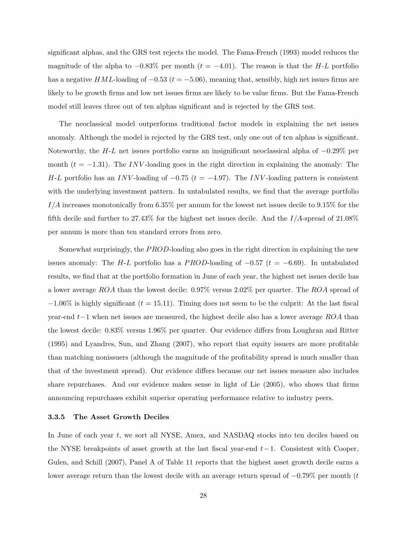
significant alphas, and the GRS test rejects the model. The Fama-French (1993) model reduces the

magnitude of the alpha to −0.83% per month (t = −4.01). The reason is that the H-L portfolio

has a negative HML-loading of −0.53 (t = −5.06), meaning that, sensibly, high net issues firms are

likely to be growth firms and low net issues firms are likely to be value firms. But the Fama-French

model still leaves three out of ten alphas significant and is rejected by the GRS test.

The neoclassical model outperforms traditional factor models in explaining the net issues

anomaly. Although the model is rejected by the GRS test, only one out of ten alphas is significant.

Noteworthy, the H-L net issues portfolio earns an insignificant neoclassical alpha of −0.29% per

month (t = −1.31). The INV -loading goes in the right direction in explaining the anomaly: The

H-L portfolio has an INV -loading of −0.75 (t = −4.97). The INV -loading pattern is consistent

with the underlying investment pattern. In untabulated results, we find that the average portfolio

I/A increases monotonically from 6.35% per annum for the lowest net issues decile to 9.15% for the

fifth decile and further to 27.43% for the highest net issues decile. And the I/A-spread of 21.08%

per annum is more than ten standard errors from zero.

Somewhat surprisingly, the PROD-loading also goes in the right direction in explaining the new

issues anomaly: The H-L portfolio has a PROD-loading of −0.57 (t = −6.69). In untabulated

results, we find that at the portfolio formation in June of each year, the highest net issues decile has

a lower average ROA than the lowest decile: 0.97% versus 2.02% per quarter. The ROA spread of

−1.06% is highly significant (t = 15.11). Timing does not seem to be the culprit: At the last fiscal

year-end t−1 when net issues are measured, the highest decile also has a lower average ROA than

the lowest decile: 0.83% versus 1.96% per quarter. Our evidence differs from Loughran and Ritter

(1995) and Lyandres, Sun, and Zhang (2007), who report that equity issuers are more profitable

than matching nonissuers (although the magnitude of the profitability spread is much smaller than

that of the investment spread). Our evidence differs because our net issues measure also includes

share repurchases. And our evidence makes sense in light of Lie (2005), who shows that firms

announcing repurchases exhibit superior operating performance relative to industry peers.

3.3.5 The Asset Growth Deciles

In June of each year t, we sort all NYSE, Amex, and NASDAQ stocks into ten deciles based on

the NYSE breakpoints of asset growth at the last fiscal year-end t−1. Consistent with Cooper,

Gulen, and Schill (2007), Panel A of Table 11 reports that the highest asset growth decile earns a

lower average return than the lowest decile with an average return spread of −0.79% per month (t

28

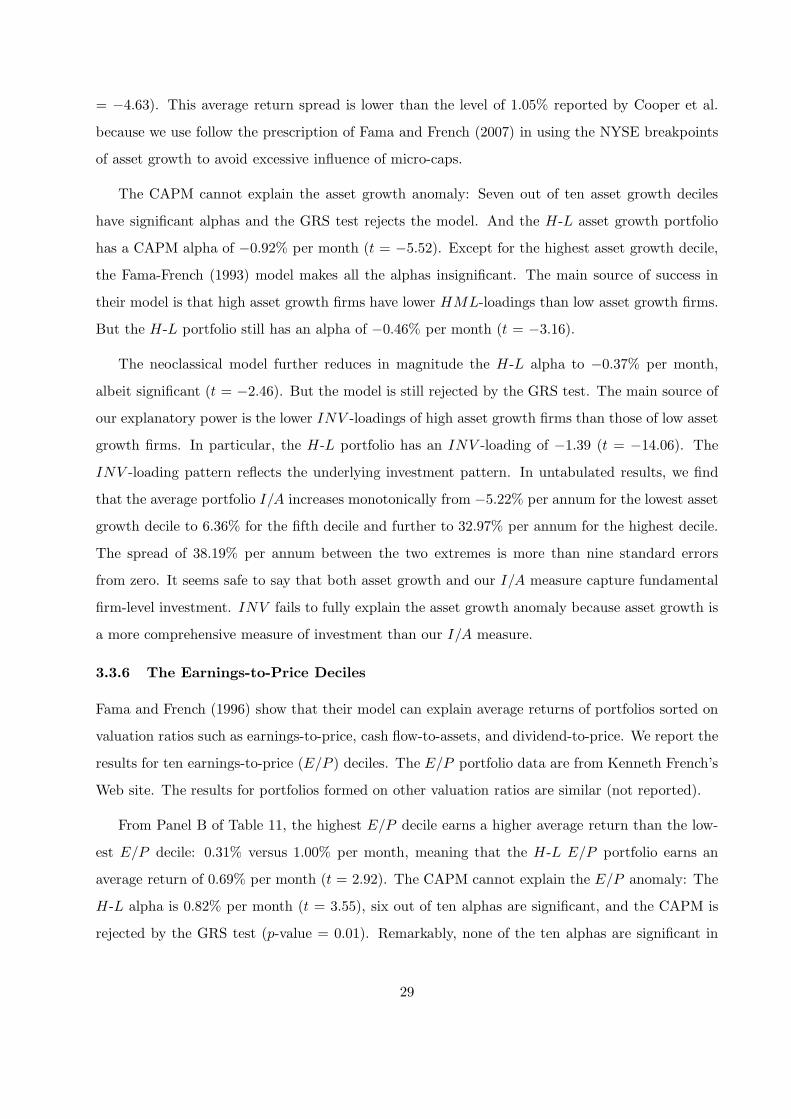
= −4.63). This average return spread is lower than the level of 1.05% reported by Cooper et al.

because we use follow the prescription of Fama and French (2007) in using the NYSE breakpoints

of asset growth to avoid excessive influence of micro-caps.

The CAPM cannot explain the asset growth anomaly: Seven out of ten asset growth deciles

have significant alphas and the GRS test rejects the model. And the H-L asset growth portfolio

has a CAPM alpha of −0.92% per month (t = −5.52). Except for the highest asset growth decile,

the Fama-French (1993) model makes all the alphas insignificant. The main source of success in

their model is that high asset growth firms have lower HML-loadings than low asset growth firms.

But the H-L portfolio still has an alpha of −0.46% per month (t = −3.16).

The neoclassical model further reduces in magnitude the H-L alpha to −0.37% per month,

albeit significant (t = −2.46). But the model is still rejected by the GRS test. The main source of

our explanatory power is the lower INV -loadings of high asset growth firms than those of low asset

growth firms. In particular, the H-L portfolio has an INV -loading of −1.39 (t = −14.06). The

INV -loading pattern reflects the underlying investment pattern. In untabulated results, we find

that the average portfolio I/A increases monotonically from −5.22% per annum for the lowest asset

growth decile to 6.36% for the fifth decile and further to 32.97% per annum for the highest decile.

The spread of 38.19% per annum between the two extremes is more than nine standard errors

from zero. It seems safe to say that both asset growth and our I/A measure capture fundamental

firm-level investment. INV fails to fully explain the asset growth anomaly because asset growth is

a more comprehensive measure of investment than our I/A measure.

3.3.6 The Earnings-to-Price Deciles

Fama and French (1996) show that their model can explain average returns of portfolios sorted on

valuation ratios such as earnings-to-price, cash flow-to-assets, and dividend-to-price. We report the

results for ten earnings-to-price (E/P ) deciles. The E/P portfolio data are from Kenneth French’s

Web site. The results for portfolios formed on other valuation ratios are similar (not reported).

From Panel B of Table 11, the highest E/P decile earns a higher average return than the low-

est E/P decile: 0.31% versus 1.00% per month, meaning that the H-L E/P portfolio earns an

average return of 0.69% per month (t = 2.92). The CAPM cannot explain the E/P anomaly: The

H-L alpha is 0.82% per month (t = 3.55), six out of ten alphas are significant, and the CAPM is

rejected by the GRS test (p-value = 0.01). Remarkably, none of the ten alphas are significant in

29

the Fama-French (1993) model, which cannot be rejected by the GRS test (p-value = 0.57). And

the H-L E/P portfolio earns a Fama-French alpha of only −0.13% per month (t = −0.90). The

main source of the extreme success for the Fama-French model is that high E/P stocks have higher

HML-loadings than low E/P stocks: The H-L portfolio has an HML-loading of 1.41 (t = 23.06).

In contrast, the performance of our neoclassical model leaves much to be desired. Three out

of ten E/P deciles have significant alphas and the GRS test rejects the model at the 1% level.

In particular, the H-L E/P portfolio earns an alpha of 0.60% per month (t = 2.46). Our model

gains some explanatory power for the E/P portfolios through their INV loadings. The H-L E/P

portfolio has an INV -loading of 0.71 (t = 3.97). In untabulated results, we confirm that the high-

est E/P decile invests less than the lowest E/P decile on average only by 2.67% per annum. The

magnitudes of the I/A spread and the subsequent INV -loading spread are not large enough to

bring our model performance up to a level comparable to the Fama-French (1993) model.

4 Cross-Sectional Regressions

We supplement our time series tests with Fama-MacBeth (1973) cross-sectional tests. To facilitate

comparison with Fama and French (2007), we follow their test design. With a few exceptions, the

general inferences from the cross-sectional tests are similar to those from our earlier time series tests.

At the end of each June from 1972 to 2006, we allocate NYSE, Amex, and NASDAQ stocks

to three size groups, micro-caps, small stocks, and big stocks. The breakpoints are the 20th and

50th percentiles of the June market cap for NYSE stocks. Panel A of Table 12 shows averages

and standard deviations of returns for the value-weighted and equal-weighted micro, small, and big

portfolios from July 1972 to December 2006. We also report time series averages of the number of

stocks and the percent of aggregate market cap in each portfolio. On average, micro-caps include

59% of all stocks, but the micro-caps account for only about 2.83% of the market value of all sample

stocks. For comparison, big stocks include 21% of all stocks but account for 91% of the total market

cap. Consequently, the micro-caps dominate the equal-weighted market returns, whereas the big

stocks dominate the value-weighted market returns.

Table 12 also reports averages of the standard deviations of the annual cross section of returns

and the anomaly variables. Fama and French (2007) observe that, for returns and all anomaly vari-

ables, the micro-cap group has the largest cross-sectional dispersion, followed by the small-stock

group, and then by the big-stock group. While replicating their evidence in our 1972–2006 sample,

30

we show that their observation also applies to our annual I/A and quarterly ROA measures. The

evidence means that micro-caps have enormous influence in cross-sectional regressions. But their

influence is more limited in time series tests because we value-weight portfolio returns.

Following Fama and French (2007), we explain the cross section of monthly returns from July

of year t to June of t+1 using anomaly variables observed in June of t or the fiscal year-end of

t−1. The exceptions are momentum and quarterly ROA, which are both updated monthly (as in

sorts). We include the market cap and book-to-market (ln(MC) and ln(B/M), respectively, both in

logs) in the regressions to proxy for the SMB- and HML-loadings. The idea is that current size

and book-to-market are more timely proxies for the loadings than unconditional regression slopes

(see Fama and French 1997). Panel A of Table 13 replicates Fama and French’s (2007, Table IV)

cross-sectional tests in our sample. In Panel B, we perform the tests after replacing their asset

growth and profitability with our I/A and quarterly ROA measures, respectively.

Table 13 shows that the value effect is reliable across all size groups in our 1972–2006 sample,

even after we include other anomaly variables such as share issuance, asset growth in cross-sectional

regressions. With Fama and French’s (2007) variable definitions (Panel A), the average slopes for

ln(B/M) are 0.26 (t = 3.14) and 0.21 (t = 2.38) for small and big stocks, respectively. The average

slope for micro-caps is smaller, 0.14 (t = 2.00). With our I/A and ROA measures (Panel B), the

average slopes for ln(B/M) are about 0.47, all of which are more than 4.2 standard errors from zero.

The average momentum slopes in Panel A are similar to those from Fama and French (2007).

The average slope for micro-caps (0.32, t = 1.89) is about half the size and more than 3.6 standard

errors below the slope for small stocks (0.77, t = 3.81) and more than 1.8 standard errors below

the slope for big stocks (0.65, t = 2.66). However, once we control for I/A and quarterly ROA, the

average momentum slope is only reliable in small stocks (0.50, t = 2.13). The slope in big stocks

is close (0.48, t = 1.80), but the slope in micro-caps is not impressive (0.18, t = 0.93).

The net stock issues show strong marginal explanatory power in all size groups in both panels

of Table 13. From Panel A, the average slopes range from −1.47 to −1.64, all of which are more

than −4.4 standard errors from zero. And the slopes differ by less than 0.6 standard errors. The

slopes vary more in Panel B from −0.64 (t = −1.46) in micro-caps to −1.96 (t = −3.30) in small

stocks. And the two are more than 1.8 standard errors apart. The dummy variable for zero net

stock issues shows more explanatory power in our tests than in those of Fama and French (2007).

In Panel A, the average slope only shows up significant in micro-caps (−0.24, t = −3.23). But the

31

slope is also reliable (−0.34, t = −2.30) for small stocks in our tests.

Consistent with Fama and French (2007), we find that the relation between accruals and average

returns is not pervasive. In Panel A, the average slope for positive accruals is only reliable in small

stocks (−1.05, t = −3.47), which is more than 2.7 standard errors from the slope in micro-caps

(−0.22, t = −1.09). Once we use our I/A and ROA in Panel B, even the strong slope in small

stocks is reduced to −0.50, which is less than 1.2 standard errors from zero. The average slopes

for negative accruals are all within 1.2 standard errors of zero in Panel A. In Panel B, the slope is

−1.00 (t = −3.37) in micro-caps but is within 0.4 standard errors of zero in small and big stocks.

We also confirm that the negative relation between asset growth and average returns is not

pervasive in cross-sectional regressions. The relation is strong in micro-caps (−1.23, t = 8.38),

substantially weaker but statistically reliable in small stocks (−0.48, t = −2.33), and probably

non-existent in big stocks (−0.43, t = −1.89). And the average slope for big stocks is −3.6 stan-

dard errors from the average slope for micro-caps. Consistent with our earlier time series tests,

I/A has a weaker explanatory power for future returns than asset growth. The average slope of

I/A is only reliable in micro-caps (−0.89, t = −3.75) and is close to zero in small and big stocks.

In untabulated results, the I/A slope for micro-caps moves up to −1.07 (t = −5.89) if we use

profitability to replace quarterly ROA in the regression. But the slopes for small and big stocks,

both around −0.15, are within 0.8 standard errors of zero. As noted, asset growth can probably

be interpreted as the most comprehensive measure of fundamental investment. Our earlier time

series results are likely to be enhanced if we use asset growth to construct the INV factor. Our

investment measure is from our earlier work in Lyandres, Sun, and Zhang (2007). And we have

not searched around for the investment measure that yields the strongest results possible.

The positive relation between (annual) profitability and average returns in the 1972–2006 sam-

ple is in line with (but somewhat weaker than) the relation in the 1963–2006 sample estimated by

Fama and French (2007). From Panel A, the average slope estimated from all stocks is reliable

(0.69, t = 2.39). But the slopes, ranging from 0.22 to 0.68 for micro-caps, small stocks, and big

stocks, are all within 1.5 standard errors of zero. In contrast, Panel B shows a much more powerful

relation between the positive quarterly ROA and average returns. The average slopes, ranging

from 5.19 in big stocks to 49.96 in micro-caps, are all more than 4.5 standard errors from zero.

And the average slope estimated from all stocks is 35.76 (t = 15.20). We also find some evidence

that negative quarterly ROA is associated with lower average returns, at least in micro-caps.

32

5 Conclusion

Motivated from neoclassical reasoning, we propose a new multi-factor model that includes the mar-

ket factor, the low-minus-high investment factor, and the high-minus-low productivity factor. We

show that the neoclassical three-factor model outperforms traditional factor models in explaining

the average returns across portfolios formed on momentum, financial distress, investment, profitabil-

ity, accruals, net stock issues, earnings surprises, and asset growth. At a minimum, the neoclassical

model seems to provide a reasonable description of the cross section of average stock returns.

5.1 Applications

Our pragmatic approach a la Fama and French (1996) means that, in principle, our neoclassical

model can be used in many applications that require estimates of expected returns. Examples in-

clude portfolio choice, portfolio performance evaluation, measurement of abnormal returns in event

studies, and the cost of capital estimates. These applications primarily depend on the empirical

performance of our model. The motivation of our factors from equilibrium asset pricing theory also

raises the likelihood that the performance of the neoclassical model can persist in the future.

Regressing the excess returns of a target portfolio on the neoclassical factors can provide the ex-

posures of the portfolio to the factors. The expected return estimate on the portfolio can be obtained

by summing the products of the regression slopes and their historical average premiums for their cor-

responding factors. The estimate then can be used to guide portfolio choice and capital budgeting

decisions. A similar procedure also can be used to evaluate the performance of a managed portfolio.

The intercept from regressing the excess return of the managed portfolio on the neoclassical factors

is the estimated average abnormal return of the portfolio. This abnormal return can be used to judge

whether the manager has done a good job in generating average returns greater than the average

returns from the passive management of combining the neoclassical factors that we have identified.

The voluminous literatures in empirical corporate finance and capital markets research in ac-

counting have used factor models to measure abnormal performance following corporate events.

The intercepts from the market regression and the Fama-French (1993) three-factor regression

are used to measure average abnormal returns. Our evidence suggests that the intercepts from the

neoclassical three-factor regressions also can do a reasonable job identifying abnormal performance.

For example, using the CAPM alpha as the measure of abnormal performance, Agrawal, Jaffe,

and Mandelker (1992) document that stockholders of acquiring firms suffer a significant loss of

33

about 10% over the five post-merger years. Because mergers and acquisitions are a form of capital

investment from the perspective of bidders, we conjecture that the post-merger underperformance

reflects the negative relation between investment and expected returns. Using the neoclassical

model is likely to yield more precise estimates of abnormal performance.

5.2 Open Questions

We take the pragmatic approach in constructing common factors motivated from neoclassical eco-

nomics. While useful in providing a parsimonious factor model for practical purposes, this approach

leaves a more fundamental question unanswered. The neoclassical factors are constructed directly

on firm characteristics. Although we show formally that these characteristics are linked to risk, our

investment-based asset pricing approach does not directly characterize the nature of or quantify

the amount of the underlying risk. (And as noted, investment-based asset pricing has so far not ad-

dressed the question why earnings and momentum anomalies are more short-lived than, for example,

value and investment anomalies.) Our basic philosophy is that, rather than determining unobserv-

able expected returns from equally unobservable risk as in traditional asset pricing literature, we

infer unobservable expected returns from observable firm characteristics and corporate policies.

We can link risk to the real economy even in investment-based partial equilibrium models. Carl-

son, Fisher, and Giammarino (2004) relate the risk of value-minus-growth strategies to operating

leverage. The higher operating leverage of value firms than that of growth firms makes the cash flows

of value firms covary more with economic downturns than the cash flows of growth firms. Zhang

(2005) argues that it is more costly for firms to downsize than to expand their productive capac-

ity. Because value firms are stuck with more unproductive capital than growth firms in recessions,

the cash flows of value firms covary more with economic downturns than the cash flows of growth

firms. Johnson (2002) shows that the curvature of log price-dividend ratio with respect to expected

growth is convex, meaning that the log price-dividend ratio is more sensitive to changes in expected

growth when expected growth is high. Sagi and Seasholes (2006) relate this expected-growth risk to

revenue growth volatility, costs, and growth options. However, because investors are not explicitly

modeled, these papers fall short of quantifying the underlying risk related to the investor behavior.

A promising direction for future research can link investment-based asset pricing to the long

run risk literature (e.g., Bansal and Yaron 2004; Bansal, Dittmar, and Lundblad 2005). The long

run risk literature characterizes the risk that investors are afraid of, whereas investment-based asset

pricing connects the risk to firm characteristics and corporate policies. General equilibrium models,

34

in which investors and firms are jointly modeled, hold the promise of understanding more funda-

mental driving forces of risk. However, because of their complex structures, constructing general

equilibrium models that can be implemented empirically remains elusive.

References

Abel, Andrew B. and Janice C. Eberly, 1994, A unified model of investment under uncertainty,American Economic Review 84 (1), 1369–1384.

Abarbanell, Jeffrey S. and Brian J. Bushee, 1998, Abnormal returns to a fundamental analysisstrategy, The Accounting Review 73 (1), 19–45.

Agrawal, Anup, Jeffrey F. Jaffe, and Gershon N. Mandelker, 1992, The post-merger performance ofacquiring firms: A re-examination of an anomaly, Journal of Finance XLVII (4), 1605–1621.

Altman, Edward I., 1968, Financial ratios, discriminant analysis and the prediction of corporatebankruptcy, Journal of Finance 23, 589–609.

Anderson, Christopher W., and Luis Garcia-Feijoo, 2006, Empirical evidence on capital invest-ment, growth options, and security Journal of Finance 61 (1), 171–194.

Ball, Ray and Philip Brown, 1968, An empirical evaluation of accounting income numbers, Journal

of Accounting Research 6, 159–178.

Ball, Ray, S. P. Kothari, and Ross L. Watts, 1993, Economic determinants of the relation betweenearnings changes and stock returns, The Accounting Review 68 (3), 622–638.

Bansal, Ravi and Amir Yaron, 2004, Risks for the long run: A potential resolution of asset pricingpuzzles, Journal of Finance 59, 1481–1509.

Bansal, Ravi, Robert F. Dittmar, and Christian T. Lundblad, 2005, Consumption, dividends, andthe cross-section of equity returns, Journal of Finance 60, 1639–1672.

Berk, Jonathan B, Richard C. Green, and Vasant Naik, 1999, Optimal investment, growth options,and security returns, Journal of Finance, 54, 1153–1607.

Bernard, Victor L. and Jacob K. Thomas, 1989, Post-earnings-announcement drift: Delayed priceresponse or risk premium? Journal of Accounting Research Supplement 27, 1–48.

Bernard, Victor L. and Jacob K. Thomas, 1990, Evidence that stock prices do not fully reflect theimplications of current earnings for future earnings, Journal of Accounting and Economics

13, 305–340.

Brealey, Richard A., Stewart C. Myers, and Franklin Allen, 2006, Principles of corporate finance,8th edition, Irwin McGraw-Hill.

Campbell, John Y. and Tuomo Vuolteenaho, 2004, Bad beta, good beta, American Economic

Review 94 (5), 1249–1275.

Campbell, John Y., Jens Hilscher, and Jan Szilagyi, 2007, In search of distress risk, working paper,Harvard University.

35

Carhart, Mark M. 1997, On persistence in mutual fund performance, Journal of Finance 52 (1),57–82.

Carlson, Murray, Adlai Fisher, and Ron Giammarino, 2004, Corporate investment and asset pricedynamics: Implications for the cross section of returns, Journal of Finance 59 (6), 2577–2603.

Carlson, Murray, Adlai Fisher, and Ron Giammarino, 2006, Corporate investment and asset pricedynamics: Implications for SEO event studies and long-run performance, Journal of Finance

61 (3), 1009–1034.

Chan, Louis K. C., Narasimhan Jegadeesh, and Josef Lakonishok, 1996, Momentum strategies,Journal of Finance 51 (5), 1681–1713.

Cochrane, John H., 1991, Production-based asset pricing and the link between stock returns andeconomic fluctuations, Journal of Finance 46, 209–237.

Cochrane, John H., 1996, A cross-sectional test of an investment-based asset pricing model, Jour-

nal of Political Economy 104, 572–621.

Cochrane, John H., 2005, Asset pricing, revised edition, Princeton University Press, Princeton,New Jersey.

Cohen, Randolph B., Paul A. Gompers, and Tuomo Vuolteenaho, 2002, Who underreacts to cash-flow news? Evidence from trading between individuals and institutions, Journal of Financial

Economics 66, 409–462.

Cooper, Ilan, 2006, Asset pricing implications of non-convex adjustment costs and irreversibilityof investment, Journal of Finance 61 (1), 139–170.

Cooper, Michael J., Huseyin Gulen, and Michael J. Schill, 2007, Asset growth and the cross-sectionof stock returns, forthcoming, Journal of Finance.

Daniel, Kent and Sheridan Titman, 1997, Evidence on the characteristics of cross sectional vari-ation in stock returns, Journal of Finance 52 (1), 1–33.

Daniel, Kent and Sheridan Titman, 2006, Market reactions to tangible and intangible information,Journal of Finance 61, 1605–1643.

DeBondt, Werner F. M. and Richard Thaler, 1985, Does the stock market overreact? Journal of

Finance 40 (3), 793–805.

Dechow, Patricia M., Amy P. Hutton, and Richard G. Sloan, 1999, An empirical assessment ofthe residual income valuation model, Journal of Accounting and Economics 26, 1–34.

Dichev, Ilia, 1998, Is the risk of bankruptcy a systematic risk? Journal of Finance 53, 1141–1148.

Fairfield, Patricia M., Scott Whisenant, and Terry Lombardi Yohn, 2003, Accrued earnings andgrowth: Implications for future profitability and market mispricing, The Accounting Review

78, 353–371.

Fama, Eugene F., 1998, Market efficiency, long-term returns, and behavioral finance, Journal of

Financial Economics 49, 283–306.

36

Fama, Eugene F. and Kenneth R. French, 1992, The cross-section of expected stock returns,Journal of Finance 47, 427–465.

Fama, Eugene F. and Kenneth R. French, 1993, Common risk factors in the returns on stocks andbonds, Journal of Financial Economics 33, 3–56.

Fama, Eugene F. and Kenneth R. French, 1995, Size and book-to-market factors in earnings andreturns, Journal of Finance L (1), 131–155.

Fama, Eugene F. and Kenneth R. French, 1996, Multifactor explanation of asset pricing anomalies,Journal of Finance LI (1), 55–84.

Fama, Eugene F. and Kenneth R. French, 1997, Industry cost of equity, Journal of Financial

Economics 43, 153–193.

Fama, Eugene F. and Kenneth R. French, 2000, Forecasting profitability and earnings, Journal of

Business 73 (2), 161–175.

Fama, Eugene F. and Kenneth R. French, 2001, Disappearing dividends: Changing firm charac-teristics or lower propensity to pay? Journal of Financial Economics 60, 3–43.

Fama, Eugene F. and Kenneth R. French, 2004, New lists: Fundamentals and survival rates,Journal of Financial Economics 73, 229–269.

Fama, Eugene F. and Kenneth R. French, 2006, Profitability, investment, and average returns,Journal of Financial Economics 82, 491–518.

Fama, Eugene F. and Kenneth R. French, 2007, Dissecting anomalies, forthcoming, Journal of

Finance.

Frankel, Richard and Charles M. C. Lee, 1998, Accounting valuation, market expectation, andcross-sectional stock returns, Journal of Accounting and Economics 25, 283–319.

Gala, Vito D., 2006, Investment and returns, working paper, London Business School.

Gibbons, Michael R., Stephen A. Ross, and Jay Shanken, 1989, A test of the efficiency of a givenportfolio, Econometrica 57 (5), 1121–1152.

Gomes, Joao F., Leonid Kogan, and Lu Zhang, 2003, Equilibrium cross section of returns, Journal

of Political Economy 111 (4), 693–732.

Gordon, Myron J., 1962, The Investment, Financing, and Valuation of the Corporation, The IrwinSeries in Economics, Homewood, Illinois.

Griffin, John M. and Michael L. Lemmon, 2002, Book-to-market equity, distress risk, and stockreturns, Journal of Finance LVII (2), 2317–2336.

Hansen, Lars Peter and Kenneth J. Singleton, 1982, Generalized instrumental variables estimationof nonlinear rational expectations models, Econometrica 50, 1269–1288.

Haugen, Robert A. and Nardin L. Baker, 1996, Commonality in the determinants of expectedstock returns, Journal of Financial Economics 41, 401–439.

Hayashi, Fumio, 1982, Tobin’s marginal and average q: A neoclassical interpretation, Economet-

rica 50 (1), 213–224.

37

Hirshleifer, David, Kewei Hou, Siew Hong Teoh, and Yinglei Zhang, 2004, Do investors overvaluefirms with bloated balance sheets? Journal of Accounting and Economics 38, 297–331.

Ikenberry, David, Josef Lakonishok, and Theo Vermaelen, 1995, Market underreaction to openmarket share repurchases, Journal of Financial Economics 39, 181–208.

Jegadeesh, Narasimhan and Sheridan Titman, 1993, Returns to buying winners and selling losers:Implications for stock market efficiency, Journal of Finance 48, 65–91.

Johnson, Timothy C., 2002, Rational momentum effects, Journal of Finance LVII (2), 585–608.

Kydland, Finn E. and Edward C. Prescott, 1982, Time to build and aggregate fluctuations, Econo-

metrica 50 (6), 1345–1370.

Lakonishok, Josef, Andrei Shleifer, Robert W. Vishny, 1994, Contrarian investment, extrapolation,and risk, Journal of Finance 49 (5), 1541–1578.

Lamont, Owen A. and Richard H. Thaler, 2003, Can the market add and subtract? Mispricing intech stock carve-outs? Journal of Political Economy 111 (2), 227–268.

Lie, Erik, 2005, Operating performance following open market share repurchase announcements,Journal of Accounting and Economics 39, 411–436.

Lintner, John, 1965, The valuation of risk assets and the selection of risky investments in stockportfolios and capital budgets, Review of Economics and Statistics 47, 13–37.

Liu, Laura Xiaolei and Lu Zhang, 2007, Momentum profits, factor pricing, and macroeconomicrisk, forthcoming, Review of Financial Studies.

Liu, Laura Xiaolei, Toni M. Whited, and Lu Zhang, 2007, Investment-based expected stock re-turns, working paper, University of Michigan.

Loughran, Tim, and Jay R. Ritter, 1995, The new issues puzzle, Journal of Finance 50, 23–51.

Lyandres, Evgeny, Le Sun, and Lu Zhang, 2007, The new issues puzzle: Testing the investment-based explanation, forthcoming, Review of Financial Studies.

Malmendier, Ulrike and Geoffrey Tate, 2005, CEO overconfidence and corporate investment, Jour-

nal of Finance 60 (6), 2661–2700.

Mitchell, Mark, Todd Pulvino, and Erik Stafford, 2002, Limited arbitrage in equity markets,Journal of Finance 57 (2), 551–584.

Ohlson, James A., 1980, Financial ratios and the probabilistic prediction of bankruptcy, Journal

of Accounting Research 18 (1), 109–131.

Piostroski, Joseph D., 2000, Value investing: The use of historical financial statement informationto separate winners from losers, Journal of Accounting Research 38, Supplement: Studies onaccounting information and the economics of the firm, 1–41.

Polk, Christopher and Paola Sapienza, 2006, The stock market and corporate investment: A testof catering theory, forthcoming, Review of Financial Studies.

Pontiff, Jeffrey and Artemiza Woodgate, 2006, Share issuance and cross-sectional returns, forth-coming, Journal of Finance.

38

Richardson, Scott A. and Richard G. Sloan, 2003, External financing and future stock returns,working paper, University of Pennsylvania.

Richardson, Scott A., Richard G. Sloan, Mark T. Soliman, and Irem Tuna, 2005, Accrual reliabil-ity, earnings persistence, and stock prices, Journal of Accounting and Economics 39, 437–485.

Ritter, Jay R., 1991, The long-run performance of initial public offerings, Journal of Finance 46,3–27.

Titman, Sheridan, K. C. John Wei, and Feixue Xie, 2004, Capital investments and stock returns,Journal of Financial and Quantitative Analysis 39, 677–700.

Sagi, Jacob S. and Mark S. Seasholes, 2007, Firm-specific attributes and the cross-section ofmomentum, Journal of Financial Economics 84, 389–434.

Sharpe, William F., 1964, Capital asset prices: A theory of market equilibrium under conditionsof risk, Journal of Finance 19, 425–442.

Sloan, Richard G., 1996, Do stock prices fully reflect information in accruals and cash flows aboutfuture earnings? The Accounting Review 71 (3), 289–315.

Spiess, Katherine D. and John Affleck-Graves, 1995, Underperformance in long-run stock returnsfollowing seasoned equity offerings, Journal of Financial Economics 38, 243–267.

Wu, Jin G., X. Frank Zhang, and Lu Zhang, 2007, The accrual anomaly: Exploring the optimalinvestment hypothesis, working paper, University of Georgia, University of Michigan, andYale School of Management.

Xie, Hong, 2001, The mispricing of abnormal accruals, The Accounting Review 76 (3), 357–373.

Xing, Yuhang, 2007, Interpreting the value effect through the Q-theory: An empirical investiga-tion, forthcoming, Review of Financial Studies.

Zhang, Lu, 2005, The value premium, Journal of Finance 60 (1), 67–103.

A A Two-Period q-Theory Model of Expected Returns

We derive the q-theory expected-returns model a la Cochrane (1991, 1996). We use a two-periodsimplification of the dynamic model derived by Liu, Whited, and Zhang (2007). See their paper for amore detailed exposition including the derivation and estimation in the infinite-horizon framework.

Firms use capital and a vector of costlessly adjustable inputs to produce a perishable outputgood. Firms choose the levels of these inputs each period to maximize their operating profits,defined as revenues minus the expenditures on these inputs. Taking the operating profits as given,firms then choose optimal investment to maximize their market value.

There are only two periods, t and t + 1. Firm j starts with capital stock kjt, invests in periodt, and produces in both t and t + 1. The firm exits at the end of period t + 1 with a liquida-tion value of (1 − δj)kjt+1, in which δj is the firm-specific rate of capital depreciation. Operating

39

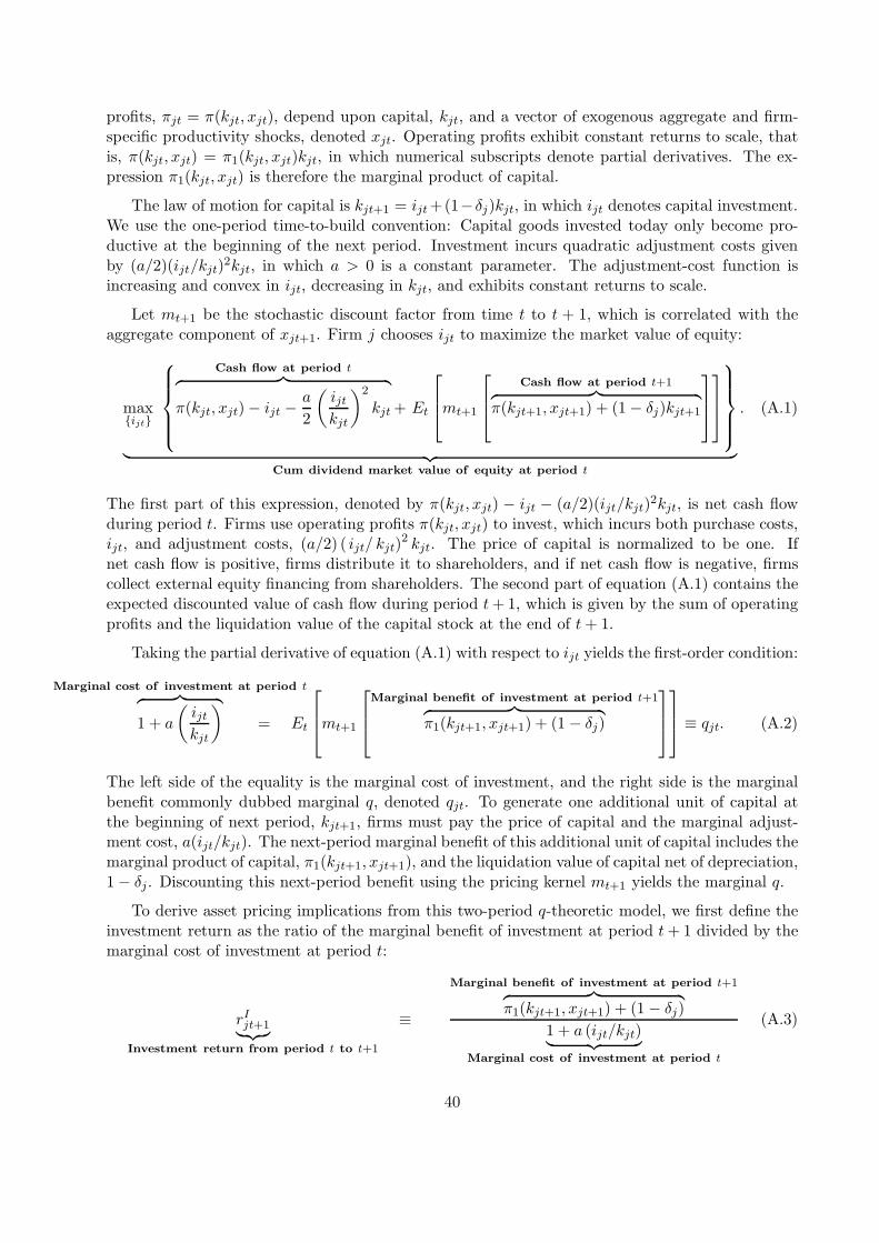
profits, πjt = π(kjt, xjt), depend upon capital, kjt, and a vector of exogenous aggregate and firm-specific productivity shocks, denoted xjt. Operating profits exhibit constant returns to scale, thatis, π(kjt, xjt) = π1(kjt, xjt)kjt, in which numerical subscripts denote partial derivatives. The ex-pression π1(kjt, xjt) is therefore the marginal product of capital.

The law of motion for capital is kjt+1 = ijt +(1−δj)kjt, in which ijt denotes capital investment.We use the one-period time-to-build convention: Capital goods invested today only become pro-ductive at the beginning of the next period. Investment incurs quadratic adjustment costs givenby (a/2)(ijt/kjt)

2kjt, in which a > 0 is a constant parameter. The adjustment-cost function isincreasing and convex in ijt, decreasing in kjt, and exhibits constant returns to scale.

Let mt+1 be the stochastic discount factor from time t to t + 1, which is correlated with theaggregate component of xjt+1. Firm j chooses ijt to maximize the market value of equity:

max{ijt}

Cash flow at period t︷ ︸︸ ︷

π(kjt, xjt) − ijt −a

2

(ijtkjt

)2

kjt + Et

mt+1

Cash flow at period t+1︷ ︸︸ ︷

π(kjt+1, xjt+1) + (1 − δj)kjt+1

︸ ︷︷ ︸

Cum dividend market value of equity at period t

. (A.1)

The first part of this expression, denoted by π(kjt, xjt) − ijt − (a/2)(ijt/kjt)2kjt, is net cash flow

during period t. Firms use operating profits π(kjt, xjt) to invest, which incurs both purchase costs,ijt, and adjustment costs, (a/2) ( ijt/ kjt)

2 kjt. The price of capital is normalized to be one. Ifnet cash flow is positive, firms distribute it to shareholders, and if net cash flow is negative, firmscollect external equity financing from shareholders. The second part of equation (A.1) contains theexpected discounted value of cash flow during period t + 1, which is given by the sum of operatingprofits and the liquidation value of the capital stock at the end of t + 1.

Taking the partial derivative of equation (A.1) with respect to ijt yields the first-order condition:

Marginal cost of investment at period t︷ ︸︸ ︷

1 + a

(ijtkjt

)

= Et

mt+1

Marginal benefit of investment at period t+1︷ ︸︸ ︷

π1(kjt+1, xjt+1) + (1 − δj)

≡ qjt. (A.2)

The left side of the equality is the marginal cost of investment, and the right side is the marginalbenefit commonly dubbed marginal q, denoted qjt. To generate one additional unit of capital atthe beginning of next period, kjt+1, firms must pay the price of capital and the marginal adjust-ment cost, a(ijt/kjt). The next-period marginal benefit of this additional unit of capital includes themarginal product of capital, π1(kjt+1, xjt+1), and the liquidation value of capital net of depreciation,1 − δj. Discounting this next-period benefit using the pricing kernel mt+1 yields the marginal q.

To derive asset pricing implications from this two-period q-theoretic model, we first define theinvestment return as the ratio of the marginal benefit of investment at period t + 1 divided by themarginal cost of investment at period t:

rIjt+1

︸ ︷︷ ︸

Investment return from period t to t+1

≡

Marginal benefit of investment at period t+1︷ ︸︸ ︷

π1(kjt+1, xjt+1) + (1 − δj)

1 + a (ijt/kjt)︸ ︷︷ ︸

Marginal cost of investment at period t

(A.3)

40

Following Cochrane (1991), we divide equation (A.2) by the marginal cost of investment:

Et

[mt+1r

Ijt+1

]= 1. (A.4)

We now show that under constant returns to scale, stock returns equal investment returns.From equation (A.1) we define the ex-dividend equity value at period t, denoted pjt, as:

pjt︸︷︷︸

Ex dividend equity value at period t

= Et

mt+1

Cash flow at period t+1︷ ︸︸ ︷

π(kjt+1, xjt+1) + (1 − δj)kjt+1

, (A.5)

The ex-dividend equity value, pjt, equals the cum-dividend equity value—the maximum in equation(A.1)—minus the net cash flow over period t. We can define the stock return, rS

jt+1, as

rSjt+1

︸ ︷︷ ︸

Stock return from period t to t+1

=

Cash flow at period t+1︷ ︸︸ ︷

π(kjt+1, xjt+1) + (1 − δj)kjt+1

Et[mt+1[π(kjt+1, xjt+1) + (1 − δj)kjt+1]]︸ ︷︷ ︸

Ex dividend equity value at period t

, (A.6)

in which the ex-dividend market value of equity in the numerator is zero in this two-period setting.

Dividing both the numerator and the denominator of equation (A.6) by kjt+1, and invoking theconstant returns assumption yields:

rSjt+1 =

π1(kjt+1, xjt+1) + (1 − δj)

Et[mt+1[π1(kjt+1, xjt+1) + (1 − δj)]]=

π1(kjt+1, xjt+1) + (1 − δj)

1 + a(ijt/kjt)= rI

jt+1.

The second equality follows from the first-order condition given by equation (A.2). Because of thisequivalence, in what follows we use rjt+1 to denote both stock and investment returns.

The marginal product of capital in the numerator of the investment-return equation (A.3) isclosely related to earnings, so expected returns increase with earnings. Specifically, earnings equalsoperating cash flows minus capital depreciation, which is the only accrual in our model. Let ejt

denote earnings, then:

ejt︸︷︷︸

Earnings

≡

Operating cash flows︷ ︸︸ ︷

π(kjt, xjt) − δjkjt︸︷︷︸

Capital depreciation

. (A.7)

Using equation (A.7) to rewrite equation (A.3) yields:

Et[rjt+1]︸ ︷︷ ︸

Expected return

=

Average product of capital︷ ︸︸ ︷

Et [πjt+1/kjt+1] + 1 − δj

1 + a(ijt/kjt)︸ ︷︷ ︸

Marginal cost of investment

=

Expected profitability︷ ︸︸ ︷

Et[ejt+1/kjt+1] + 1

1 + a(ijt/kjt)︸ ︷︷ ︸

Marginal cost of investment

(A.8)

Given the market-to-book ratio in the denominator, equation (A.8) predicts that the expectedreturn increases with the expected profitability. Haugen and Baker (1996) and Fama and French(2006) show that, controlling for market valuation ratios, firms with high expected profitability

41

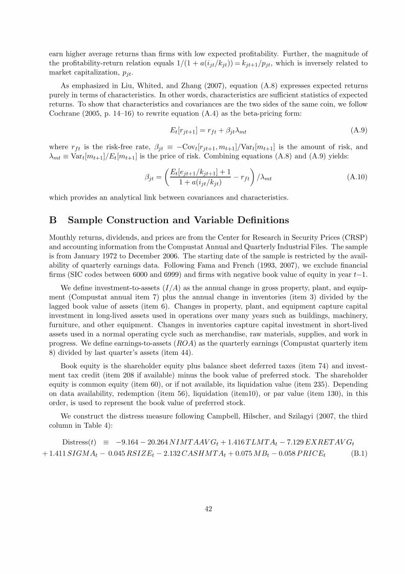
earn higher average returns than firms with low expected profitability. Further, the magnitude ofthe profitability-return relation equals 1/(1 + a(ijt/kjt)) = kjt+1/pjt, which is inversely related tomarket capitalization, pjt.

As emphasized in Liu, Whited, and Zhang (2007), equation (A.8) expresses expected returnspurely in terms of characteristics. In other words, characteristics are sufficient statistics of expectedreturns. To show that characteristics and covariances are the two sides of the same coin, we followCochrane (2005, p. 14–16) to rewrite equation (A.4) as the beta-pricing form:

Et[rjt+1] = rft + βjtλmt (A.9)

where rft is the risk-free rate, βjt ≡ −Covt[rjt+1,mt+1]/Vart[mt+1] is the amount of risk, andλmt ≡ Vart[mt+1]/Et[mt+1] is the price of risk. Combining equations (A.8) and (A.9) yields:

βjt =

(Et[ejt+1/kjt+1] + 1

1 + a(ijt/kjt)− rft

)

/λmt (A.10)

which provides an analytical link between covariances and characteristics.

B Sample Construction and Variable Definitions

Monthly returns, dividends, and prices are from the Center for Research in Security Prices (CRSP)and accounting information from the Compustat Annual and Quarterly Industrial Files. The sampleis from January 1972 to December 2006. The starting date of the sample is restricted by the avail-ability of quarterly earnings data. Following Fama and French (1993, 2007), we exclude financialfirms (SIC codes between 6000 and 6999) and firms with negative book value of equity in year t−1.

We define investment-to-assets (I/A) as the annual change in gross property, plant, and equip-ment (Compustat annual item 7) plus the annual change in inventories (item 3) divided by thelagged book value of assets (item 6). Changes in property, plant, and equipment capture capitalinvestment in long-lived assets used in operations over many years such as buildings, machinery,furniture, and other equipment. Changes in inventories capture capital investment in short-livedassets used in a normal operating cycle such as merchandise, raw materials, supplies, and work inprogress. We define earnings-to-assets (ROA) as the quarterly earnings (Compustat quarterly item8) divided by last quarter’s assets (item 44).

Book equity is the shareholder equity plus balance sheet deferred taxes (item 74) and invest-ment tax credit (item 208 if available) minus the book value of preferred stock. The shareholderequity is common equity (item 60), or if not available, its liquidation value (item 235). Dependingon data availability, redemption (item 56), liquidation (item10), or par value (item 130), in thisorder, is used to represent the book value of preferred stock.

We construct the distress measure following Campbell, Hilscher, and Szilagyi (2007, the thirdcolumn in Table 4):

Distress(t) ≡ −9.164 − 20.264NIMTAAV Gt + 1.416TLMTAt − 7.129EXRETAV Gt

+ 1.411SIGMAt − 0.045RSIZEt − 2.132CASHMTAt + 0.075MBt − 0.058PRICEt (B.1)

42

in which

NIMTAAV Gt−1,t−12 ≡

1 − φ2

1 − φ12

(NIMTAt−1,t−3 + · · · + φ9NIMTAt−10,t−12

)(B.2)

EXRETAV Gt−1,t−12 ≡

1 − φ

1 − φ12

(EXRETt−1 + · · · + φ11EXRETt−12

)(B.3)

The coefficient φ = 2−1/3, meaning that the weight is halved each quarter. NIMTA is net in-come (COMPUSTAT quarterly item 69) divided by the sum of market equity and total liabilities(item 54). The moving average NIMTAAV G is designed to capture the idea that a long his-tory of losses is a better predictor of bankruptcy than one large quarterly loss in a single month.EXRET ≡ log(1 + Rit)− log(1 + RS&P500,t) is the monthly log excess return on each firm’s equityrelative to the S&P 500 index. The moving average EXRETAV G is designed to capture the ideathat a sustained decline in stock market value is a better predictor of bankruptcy than a suddenstock price decline in a single month. TLMTA is the ratio of total liabilities divided by the sum ofmarket equity and total liabilities. SIGMA is the volatility of each firm’s daily stock return overthe past three months. RSIZE is the relative size of each firm measured as the log ratio of itsmarket equity to that of the S&P 500 index. CASHMTA, used to capture the liquidity position ofthe firm, is the ratio of cash and short-term investments divided by the sum of market equity andtotal liabilities. MB is the market-to-book equity. PRICE is the log price per share of the firm.

Following Fama and French (2007), we measure accruals as the change of operating workingcapital per split-adjusted share from year t−1 to t divided by book equity per split-adjusted shareat year t. Operating working capital is current assets (Compustat annual item 4) minus cash andshort-term investment (item 1) minus current liabilities (item 5) plus debt in current liabilities(item 34). And we measure net stock issues as the the natural log of the ratio of the split-adjustedshares outstanding at the fiscal year-end in t−1 divided by the split-adjusted shares outstanding atthe fiscal year-end in t−2. The split-adjusted shares outstanding is Compustat shares outstanding(25) times the Compustat adjustment factor (item 27). Profitability is earnings (income beforeextraordinary, item 18) minus dividends on preferred stocks (item 19), if available, plus incomestatement deferred taxes (item 50), if available, in t−1, divided by book equity for t−1.

In time series tests with sorts, we follow Cooper, Gulen, and Schill (2007) and measure assetgrowth of year t as the change of total assets (Compustat annual item 6) from t−1 to t dividedby the total assets from year t−1. To facilitate comparison with Fama and French (2007), we usetheir definition of asset growth in cross-sectional regressions. Specifically, we measure asset growthof year t as the natural log of the ratio of assets per split-adjusted share at the fiscal year-end int−1 divided by assets per split-adjusted share at the fiscal year-end in t−2.

Following Chan, Jegadeesh, and Lakonishok (1996), we define SUE as the unexpected earnings(the change in quarterly earnings per share from its value four quarters before) divided by thestandard deviation of unexpected earnings over the prior eight quarters.

43

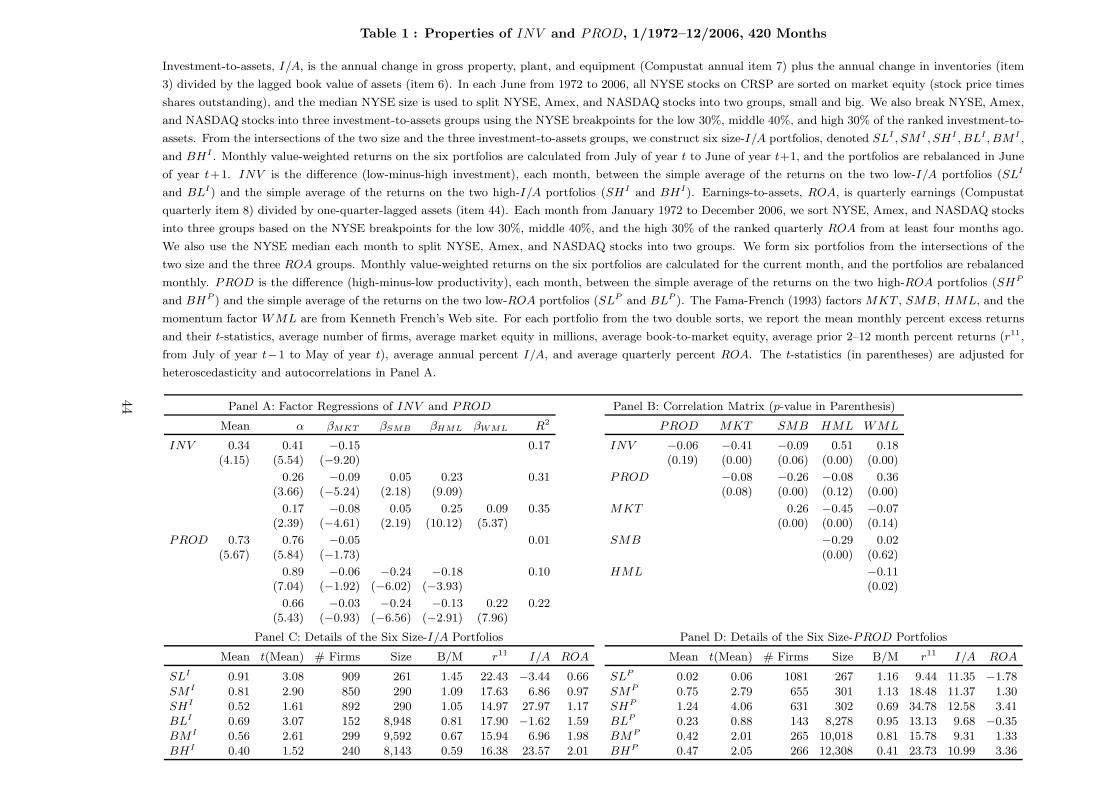
Table 1 : Properties of INV and PROD, 1/1972–12/2006, 420 Months

Investment-to-assets, I/A, is the annual change in gross property, plant, and equipment (Compustat annual item 7) plus the annual change in inventories (item

3) divided by the lagged book value of assets (item 6). In each June from 1972 to 2006, all NYSE stocks on CRSP are sorted on market equity (stock price times

shares outstanding), and the median NYSE size is used to split NYSE, Amex, and NASDAQ stocks into two groups, small and big. We also break NYSE, Amex,

and NASDAQ stocks into three investment-to-assets groups using the NYSE breakpoints for the low 30%, middle 40%, and high 30% of the ranked investment-to-

assets. From the intersections of the two size and the three investment-to-assets groups, we construct six size-I/A portfolios, denoted SLI , SMI , SHI , BLI , BMI ,

and BHI . Monthly value-weighted returns on the six portfolios are calculated from July of year t to June of year t+1, and the portfolios are rebalanced in June

of year t+1. INV is the difference (low-minus-high investment), each month, between the simple average of the returns on the two low-I/A portfolios (SLI

and BLI) and the simple average of the returns on the two high-I/A portfolios (SHI and BHI). Earnings-to-assets, ROA, is quarterly earnings (Compustat

quarterly item 8) divided by one-quarter-lagged assets (item 44). Each month from January 1972 to December 2006, we sort NYSE, Amex, and NASDAQ stocks

into three groups based on the NYSE breakpoints for the low 30%, middle 40%, and the high 30% of the ranked quarterly ROA from at least four months ago.

We also use the NYSE median each month to split NYSE, Amex, and NASDAQ stocks into two groups. We form six portfolios from the intersections of the

two size and the three ROA groups. Monthly value-weighted returns on the six portfolios are calculated for the current month, and the portfolios are rebalanced

monthly. PROD is the difference (high-minus-low productivity), each month, between the simple average of the returns on the two high-ROA portfolios (SHP

and BHP ) and the simple average of the returns on the two low-ROA portfolios (SLP and BLP ). The Fama-French (1993) factors MKT , SMB, HML, and the

momentum factor WML are from Kenneth French’s Web site. For each portfolio from the two double sorts, we report the mean monthly percent excess returns

and their t-statistics, average number of firms, average market equity in millions, average book-to-market equity, average prior 2–12 month percent returns (r11,

from July of year t−1 to May of year t), average annual percent I/A, and average quarterly percent ROA. The t-statistics (in parentheses) are adjusted for

heteroscedasticity and autocorrelations in Panel A.

Panel A: Factor Regressions of INV and PROD Panel B: Correlation Matrix (p-value in Parenthesis)

Mean α βMKT βSMB βHML βWML R2 PROD MKT SMB HML WML

INV 0.34 0.41 −0.15 0.17 INV −0.06 −0.41 −0.09 0.51 0.18(4.15) (5.54) (−9.20) (0.19) (0.00) (0.06) (0.00) (0.00)

0.26 −0.09 0.05 0.23 0.31 PROD −0.08 −0.26 −0.08 0.36(3.66) (−5.24) (2.18) (9.09) (0.08) (0.00) (0.12) (0.00)

0.17 −0.08 0.05 0.25 0.09 0.35 MKT 0.26 −0.45 −0.07(2.39) (−4.61) (2.19) (10.12) (5.37) (0.00) (0.00) (0.14)

PROD 0.73 0.76 −0.05 0.01 SMB −0.29 0.02(5.67) (5.84) (−1.73) (0.00) (0.62)

0.89 −0.06 −0.24 −0.18 0.10 HML −0.11(7.04) (−1.92) (−6.02) (−3.93) (0.02)

0.66 −0.03 −0.24 −0.13 0.22 0.22(5.43) (−0.93) (−6.56) (−2.91) (7.96)

Panel C: Details of the Six Size-I/A Portfolios Panel D: Details of the Six Size-PROD Portfolios

Mean t(Mean) # Firms Size B/M r11 I/A ROA Mean t(Mean) # Firms Size B/M r11 I/A ROA

SLI 0.91 3.08 909 261 1.45 22.43 −3.44 0.66 SLP 0.02 0.06 1081 267 1.16 9.44 11.35 −1.78

SMI 0.81 2.90 850 290 1.09 17.63 6.86 0.97 SMP 0.75 2.79 655 301 1.13 18.48 11.37 1.30SHI 0.52 1.61 892 290 1.05 14.97 27.97 1.17 SHP 1.24 4.06 631 302 0.69 34.78 12.58 3.41BLI 0.69 3.07 152 8,948 0.81 17.90 −1.62 1.59 BLP 0.23 0.88 143 8,278 0.95 13.13 9.68 −0.35BMI 0.56 2.61 299 9,592 0.67 15.94 6.96 1.98 BMP 0.42 2.01 265 10,018 0.81 15.78 9.31 1.33BHI 0.40 1.52 240 8,143 0.59 16.38 23.57 2.01 BHP 0.47 2.05 266 12,308 0.41 23.73 10.99 3.36

44

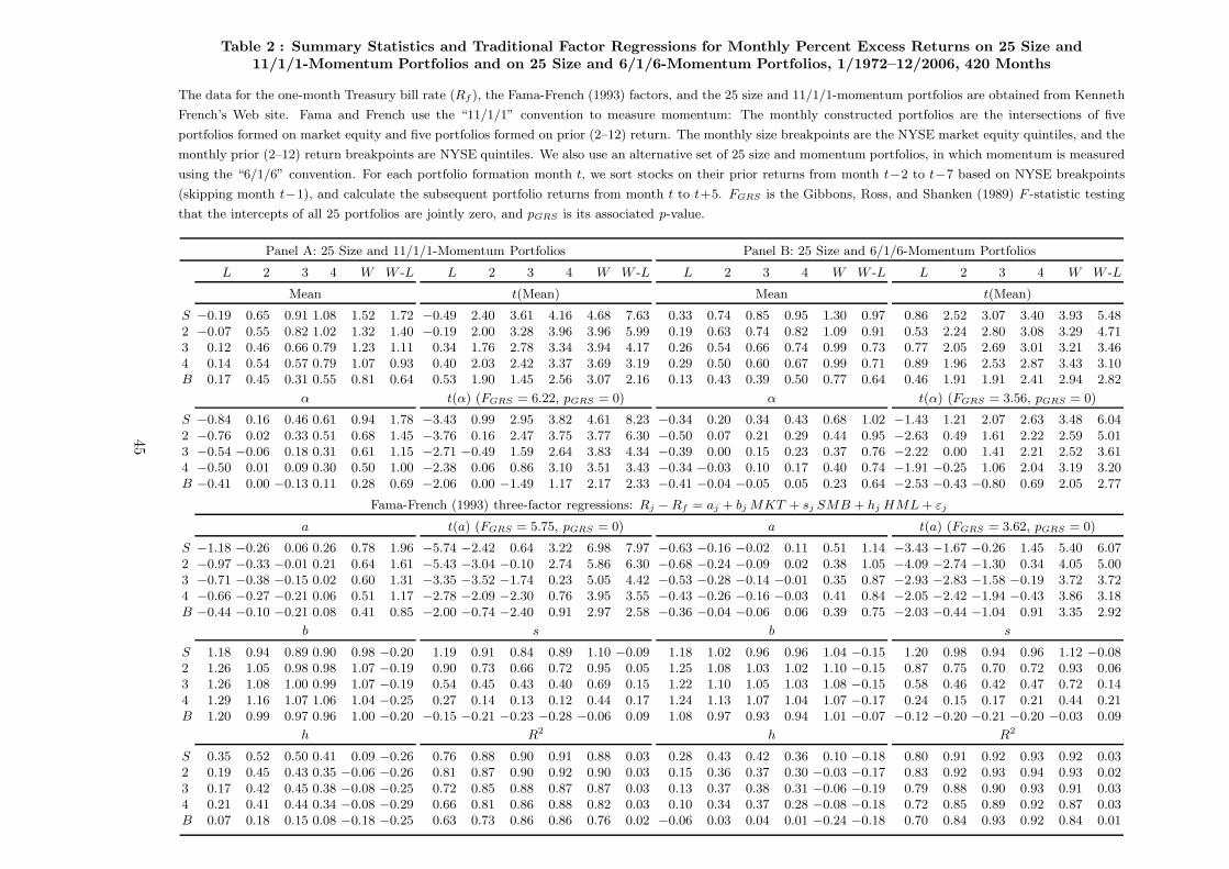
Table 2 : Summary Statistics and Traditional Factor Regressions for Monthly Percent Excess Returns on 25 Size and11/1/1-Momentum Portfolios and on 25 Size and 6/1/6-Momentum Portfolios, 1/1972–12/2006, 420 Months

The data for the one-month Treasury bill rate (Rf ), the Fama-French (1993) factors, and the 25 size and 11/1/1-momentum portfolios are obtained from Kenneth

French’s Web site. Fama and French use the “11/1/1” convention to measure momentum: The monthly constructed portfolios are the intersections of five

portfolios formed on market equity and five portfolios formed on prior (2–12) return. The monthly size breakpoints are the NYSE market equity quintiles, and the

monthly prior (2–12) return breakpoints are NYSE quintiles. We also use an alternative set of 25 size and momentum portfolios, in which momentum is measured

using the “6/1/6” convention. For each portfolio formation month t, we sort stocks on their prior returns from month t−2 to t−7 based on NYSE breakpoints

(skipping month t−1), and calculate the subsequent portfolio returns from month t to t+5. FGRS is the Gibbons, Ross, and Shanken (1989) F -statistic testing

that the intercepts of all 25 portfolios are jointly zero, and pGRS is its associated p-value.

Panel A: 25 Size and 11/1/1-Momentum Portfolios Panel B: 25 Size and 6/1/6-Momentum Portfolios

L 2 3 4 W W -L L 2 3 4 W W -L L 2 3 4 W W -L L 2 3 4 W W -L

Mean t(Mean) Mean t(Mean)

S −0.19 0.65 0.91 1.08 1.52 1.72 −0.49 2.40 3.61 4.16 4.68 7.63 0.33 0.74 0.85 0.95 1.30 0.97 0.86 2.52 3.07 3.40 3.93 5.482 −0.07 0.55 0.82 1.02 1.32 1.40 −0.19 2.00 3.28 3.96 3.96 5.99 0.19 0.63 0.74 0.82 1.09 0.91 0.53 2.24 2.80 3.08 3.29 4.713 0.12 0.46 0.66 0.79 1.23 1.11 0.34 1.76 2.78 3.34 3.94 4.17 0.26 0.54 0.66 0.74 0.99 0.73 0.77 2.05 2.69 3.01 3.21 3.464 0.14 0.54 0.57 0.79 1.07 0.93 0.40 2.03 2.42 3.37 3.69 3.19 0.29 0.50 0.60 0.67 0.99 0.71 0.89 1.96 2.53 2.87 3.43 3.10B 0.17 0.45 0.31 0.55 0.81 0.64 0.53 1.90 1.45 2.56 3.07 2.16 0.13 0.43 0.39 0.50 0.77 0.64 0.46 1.91 1.91 2.41 2.94 2.82

α t(α) (FGRS = 6.22, pGRS = 0) α t(α) (FGRS = 3.56, pGRS = 0)

S −0.84 0.16 0.46 0.61 0.94 1.78 −3.43 0.99 2.95 3.82 4.61 8.23 −0.34 0.20 0.34 0.43 0.68 1.02 −1.43 1.21 2.07 2.63 3.48 6.042 −0.76 0.02 0.33 0.51 0.68 1.45 −3.76 0.16 2.47 3.75 3.77 6.30 −0.50 0.07 0.21 0.29 0.44 0.95 −2.63 0.49 1.61 2.22 2.59 5.013 −0.54 −0.06 0.18 0.31 0.61 1.15 −2.71 −0.49 1.59 2.64 3.83 4.34 −0.39 0.00 0.15 0.23 0.37 0.76 −2.22 0.00 1.41 2.21 2.52 3.614 −0.50 0.01 0.09 0.30 0.50 1.00 −2.38 0.06 0.86 3.10 3.51 3.43 −0.34 −0.03 0.10 0.17 0.40 0.74 −1.91 −0.25 1.06 2.04 3.19 3.20B −0.41 0.00 −0.13 0.11 0.28 0.69 −2.06 0.00 −1.49 1.17 2.17 2.33 −0.41 −0.04 −0.05 0.05 0.23 0.64 −2.53 −0.43 −0.80 0.69 2.05 2.77

Fama-French (1993) three-factor regressions: Rj − Rf = aj + bj MKT + sj SMB + hj HML + εj

a t(a) (FGRS = 5.75, pGRS = 0) a t(a) (FGRS = 3.62, pGRS = 0)

S −1.18 −0.26 0.06 0.26 0.78 1.96 −5.74 −2.42 0.64 3.22 6.98 7.97 −0.63 −0.16 −0.02 0.11 0.51 1.14 −3.43 −1.67 −0.26 1.45 5.40 6.072 −0.97 −0.33 −0.01 0.21 0.64 1.61 −5.43 −3.04 −0.10 2.74 5.86 6.30 −0.68 −0.24 −0.09 0.02 0.38 1.05 −4.09 −2.74 −1.30 0.34 4.05 5.003 −0.71 −0.38 −0.15 0.02 0.60 1.31 −3.35 −3.52 −1.74 0.23 5.05 4.42 −0.53 −0.28 −0.14 −0.01 0.35 0.87 −2.93 −2.83 −1.58 −0.19 3.72 3.724 −0.66 −0.27 −0.21 0.06 0.51 1.17 −2.78 −2.09 −2.30 0.76 3.95 3.55 −0.43 −0.26 −0.16 −0.03 0.41 0.84 −2.05 −2.42 −1.94 −0.43 3.86 3.18B −0.44 −0.10 −0.21 0.08 0.41 0.85 −2.00 −0.74 −2.40 0.91 2.97 2.58 −0.36 −0.04 −0.06 0.06 0.39 0.75 −2.03 −0.44 −1.04 0.91 3.35 2.92

b s b s

S 1.18 0.94 0.89 0.90 0.98 −0.20 1.19 0.91 0.84 0.89 1.10 −0.09 1.18 1.02 0.96 0.96 1.04 −0.15 1.20 0.98 0.94 0.96 1.12 −0.082 1.26 1.05 0.98 0.98 1.07 −0.19 0.90 0.73 0.66 0.72 0.95 0.05 1.25 1.08 1.03 1.02 1.10 −0.15 0.87 0.75 0.70 0.72 0.93 0.063 1.26 1.08 1.00 0.99 1.07 −0.19 0.54 0.45 0.43 0.40 0.69 0.15 1.22 1.10 1.05 1.03 1.08 −0.15 0.58 0.46 0.42 0.47 0.72 0.144 1.29 1.16 1.07 1.06 1.04 −0.25 0.27 0.14 0.13 0.12 0.44 0.17 1.24 1.13 1.07 1.04 1.07 −0.17 0.24 0.15 0.17 0.21 0.44 0.21B 1.20 0.99 0.97 0.96 1.00 −0.20 −0.15 −0.21 −0.23 −0.28 −0.06 0.09 1.08 0.97 0.93 0.94 1.01 −0.07 −0.12 −0.20 −0.21 −0.20 −0.03 0.09

h R2 h R2

S 0.35 0.52 0.50 0.41 0.09 −0.26 0.76 0.88 0.90 0.91 0.88 0.03 0.28 0.43 0.42 0.36 0.10 −0.18 0.80 0.91 0.92 0.93 0.92 0.032 0.19 0.45 0.43 0.35 −0.06 −0.26 0.81 0.87 0.90 0.92 0.90 0.03 0.15 0.36 0.37 0.30 −0.03 −0.17 0.83 0.92 0.93 0.94 0.93 0.023 0.17 0.42 0.45 0.38 −0.08 −0.25 0.72 0.85 0.88 0.87 0.87 0.03 0.13 0.37 0.38 0.31 −0.06 −0.19 0.79 0.88 0.90 0.93 0.91 0.034 0.21 0.41 0.44 0.34 −0.08 −0.29 0.66 0.81 0.86 0.88 0.82 0.03 0.10 0.34 0.37 0.28 −0.08 −0.18 0.72 0.85 0.89 0.92 0.87 0.03B 0.07 0.18 0.15 0.08 −0.18 −0.25 0.63 0.73 0.86 0.86 0.76 0.02 −0.06 0.03 0.04 0.01 −0.24 −0.18 0.70 0.84 0.93 0.92 0.84 0.01

45

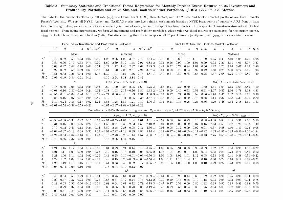
Table 3 : Summary Statistics and Traditional Factor Regressions for Monthly Percent Excess Returns on 25 Investment andProfitability Portfolios and on 25 Size and Book-to-Market Portfolios, 1/1972–12/2006, 420 Months

The data for the one-month Treasury bill rate (Rf ), the Fama-French (1993) three factors, and the 25 size and book-to-market portfolios are from Kenneth

French’s Web site. We sort all NYSE, Amex, and NASDAQ stocks into five quintiles each month based on NYSE breakpoints of quarterly ROA from at least

four months ago. Also, we sort all stocks independently in June of each year into five quintiles based on NYSE breakpoints of investment-to-assets at the last

fiscal yearend. From taking intersections, we form 25 investment and profitability portfolios, whose value-weighted returns are calculated for the current month.

FGRS is the Gibbons, Ross, and Shanken (1989) F -statistic testing that the intercepts of all 25 portfolios are jointly zero, and pGRS is its associated p-value.

Panel A: 25 Investment and Profitability Portfolios Panel B: 25 Size and Book-to-Market Portfolios

LP 2 3 4 HP H-LP LP 2 3 4 HP H-LP L 2 3 4 H H-L L 2 3 4 H H-L

Mean t(Mean) Mean t(Mean)

LI 0.42 0.82 0.55 0.93 0.82 0.40 1.26 2.96 1.92 3.57 2.79 1.64 S 0.10 0.81 0.88 1.07 1.19 1.09 0.25 2.40 3.10 4.05 4.21 5.082 0.54 0.66 0.76 0.38 0.74 0.20 1.60 2.39 3.12 1.58 2.97 0.83 2 0.34 0.66 0.90 1.00 1.04 0.69 0.93 2.27 3.51 4.06 3.77 3.273 0.08 0.47 0.42 0.74 0.62 0.54 0.24 1.72 1.43 2.97 2.62 2.29 3 0.41 0.72 0.74 0.84 1.07 0.66 1.22 2.70 3.14 3.67 4.12 2.864 −0.22 0.32 0.58 0.59 0.60 0.82 −0.64 1.20 2.05 2.31 2.24 3.37 4 0.51 0.58 0.79 0.84 0.92 0.42 1.68 2.28 3.30 3.72 3.65 1.93HI

−0.51 0.32 0.21 0.42 0.66 1.17 −1.39 1.01 0.67 1.46 2.15 4.81 B 0.40 0.61 0.59 0.65 0.65 0.25 1.67 2.68 2.75 3.13 2.80 1.20

H-LI−0.93 −0.49−0.34−0.51−0.16 −4.30−2.24−1.38 −2.84−0.87

α t(α) (FGRS = 3.17, pGRS = 0) α t(α) (FGRS = 4.25, pGRS = 0)

LI−0.18 0.30 0.04 0.43 0.25 0.43 −0.89 1.90 0.25 2.95 1.60 1.75 S −0.63 0.21 0.37 0.60 0.70 1.32 −2.61 1.03 2.15 3.64 3.82 7.10

2 −0.08 0.16 0.30 −0.09 0.24 0.32 −0.38 1.03 2.17 −0.76 1.80 1.33 2 −0.38 0.09 0.40 0.53 0.53 0.91 −2.07 0.57 2.96 3.78 3.18 4.833 −0.55 0.01 −0.09 0.26 0.14 0.69 −2.71 0.06−0.46 1.99 1.31 3.00 3 −0.27 0.17 0.27 0.40 0.59 0.86 −1.74 1.45 2.32 3.16 3.71 3.964 −0.85 −0.16 0.07 0.07 0.04 0.89 −4.19−1.01 0.41 0.55 0.36 3.87 4 −0.13 0.04 0.30 0.39 0.45 0.58 −1.14 0.37 2.68 3.33 3.06 2.82

HI−1.19 −0.24−0.35−0.17 0.02 1.22 −5.53−1.25−1.86 −1.21 0.19 4.96 B −0.11 0.13 0.16 0.26 0.25 0.36 −1.29 1.48 1.54 2.18 1.61 1.81

H-LI−1.01 −0.54−0.39−0.59−0.23 −4.67−2.47−1.68 −3.26−1.22

Fama-French (1993) three-factor regressions: Rj − Rf = aj + bj MKT + sj SMB + hj HML + εj

a t(a) (FGRS = 3.32, pGRS = 0) a t(a) (FGRS = 3.08, pGRS = 0)

LI−0.53 −0.08−0.30 0.22 0.16 0.69 −2.97−0.55−1.64 1.64 1.01 3.01 S −0.52 0.08 0.09 0.23 0.16 0.68 −4.48 0.88 1.35 3.31 2.16 5.50

2 −0.31 −0.16 0.05 −0.26 0.22 0.52 −1.56−0.97 0.35 −2.03 1.50 2.10 2 −0.21 −0.12 0.05 0.09−0.07 0.15 −2.63−1.55 0.67 1.23 −0.93 1.423 −0.70 −0.42−0.44 0.13 0.24 0.94 −3.59−2.45−2.28 0.95 2.17 4.36 3 −0.03 −0.05−0.12−0.09−0.02 0.01 −0.37−0.58−1.50 −1.13−0.22 0.084 −1.02 −0.37−0.19 0.05 0.30 1.32 −4.97−2.22−1.19 0.39 2.84 5.74 4 0.11 −0.17−0.07−0.05−0.11 −0.22 1.33−1.87−0.83 −0.56−1.06−1.84HI

−1.24 −0.54−0.67−0.16 0.19 1.43 −6.15−2.78−3.26 −1.14 1.57 6.08 B 0.17 0.04 −0.02−0.13−0.26 −0.43 2.75 0.55−0.28 −1.75−2.34−3.34

H-LI−0.70 −0.46−0.37−0.39 0.03 −3.45−2.06−1.44 −2.16 0.19

b s b s

LI 1.21 1.15 1.12 1.06 1.14 −0.08 0.64 0.29 0.21 0.14 0.19 −0.45 S 1.08 0.95 0.91 0.88 0.99 −0.09 1.32 1.29 1.06 0.99 1.05−0.272 1.21 1.11 1.00 0.99 0.98 −0.23 0.49 0.16 0.13 0.10 0.04 −0.45 2 1.13 1.04 0.99 0.97 1.09 −0.04 0.98 0.86 0.74 0.71 0.85−0.123 1.21 1.06 1.14 1.02 0.92 −0.29 0.44 0.25 0.10 −0.01−0.06 −0.50 3 1.06 1.08 1.02 1.01 1.12 0.05 0.73 0.51 0.41 0.38 0.51−0.224 1.22 1.02 1.09 1.05 1.00 −0.21 0.48 0.15 0.20 −0.09−0.08 −0.56 4 1.06 1.11 1.10 1.04 1.16 0.10 0.40 0.22 0.18 0.19 0.18−0.21HI 1.26 1.19 1.16 1.16 1.15 −0.11 0.51 0.33 0.40 0.02 0.17 −0.35 B 0.95 1.05 1.00 1.00 1.05 0.10 −0.29−0.22−0.23 −0.21−0.11 0.18

H-LI 0.05 0.04 0.04 0.10 0.01 −0.13 0.04 0.19 −0.13−0.02

h R2 h R2

LI 0.46 0.54 0.50 0.29 0.11 −0.34 0.72 0.75 0.64 0.73 0.73 0.09 S −0.34 0.04 0.28 0.44 0.68 1.02 0.92 0.94 0.95 0.94 0.94 0.702 0.29 0.47 0.37 0.25 0.03 −0.25 0.68 0.67 0.72 0.74 0.75 0.13 2 −0.39 0.19 0.45 0.58 0.79 1.18 0.95 0.94 0.93 0.93 0.94 0.783 0.18 0.63 0.52 0.20−0.13 −0.31 0.68 0.64 0.61 0.72 0.78 0.18 3 −0.47 0.27 0.53 0.69 0.86 1.32 0.95 0.90 0.89 0.89 0.88 0.794 0.19 0.29 0.37 0.04−0.39 −0.57 0.68 0.65 0.66 0.78 0.86 0.19 4 −0.43 0.29 0.55 0.64 0.83 1.25 0.94 0.88 0.87 0.88 0.86 0.76

HI 0.00 0.41 0.45 0.00−0.28 −0.28 0.71 0.65 0.65 0.79 0.84 0.06 B −0.39 0.16 0.31 0.63 0.80 1.19 0.94 0.89 0.85 0.88 0.78 0.62H-LI

−0.46 −0.12−0.05−0.30−0.39 0.10 0.01 0.02 0.09 0.09

46

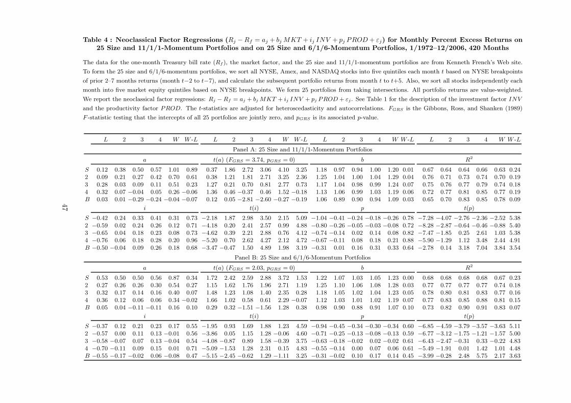
Table 4 : Neoclassical Factor Regressions (Rj − Rf = aj + bj MKT + ij INV + pj PROD + εj) for Monthly Percent Excess Returns on25 Size and 11/1/1-Momentum Portfolios and on 25 Size and 6/1/6-Momentum Portfolios, 1/1972–12/2006, 420 Months

The data for the one-month Treasury bill rate (Rf ), the market factor, and the 25 size and 11/1/1-momentum portfolios are from Kenneth French’s Web site.

To form the 25 size and 6/1/6-momentum portfolios, we sort all NYSE, Amex, and NASDAQ stocks into five quintiles each month t based on NYSE breakpoints

of prior 2–7 months returns (month t−2 to t−7), and calculate the subsequent portfolio returns from month t to t+5. Also, we sort all stocks independently each

month into five market equity quintiles based on NYSE breakpoints. We form 25 portfolios from taking intersections. All portfolio returns are value-weighted.

We report the neoclassical factor regressions: Rj − Rf = aj + bj MKT + ij INV + pj PROD + εj . See Table 1 for the description of the investment factor INV

and the productivity factor PROD. The t-statistics are adjusted for heteroscedasticity and autocorrelations. FGRS is the Gibbons, Ross, and Shanken (1989)

F -statistic testing that the intercepts of all 25 portfolios are jointly zero, and pGRS is its associated p-value.

L 2 3 4 W W -L L 2 3 4 W W -L L 2 3 4 W W -L L 2 3 4 W W -L

Panel A: 25 Size and 11/1/1-Momentum Portfolios

a t(a) (FGRS = 3.74, pGRS = 0) b R2

S 0.12 0.38 0.50 0.57 1.01 0.89 0.37 1.86 2.72 3.06 4.10 3.25 1.18 0.97 0.94 1.00 1.20 0.01 0.67 0.64 0.64 0.66 0.63 0.242 0.09 0.21 0.27 0.42 0.70 0.61 0.38 1.21 1.81 2.71 3.25 2.36 1.25 1.04 1.00 1.04 1.29 0.04 0.76 0.71 0.73 0.74 0.70 0.193 0.28 0.03 0.09 0.11 0.51 0.23 1.27 0.21 0.70 0.81 2.77 0.73 1.17 1.04 0.98 0.99 1.24 0.07 0.75 0.76 0.77 0.79 0.74 0.184 0.32 0.07 −0.04 0.05 0.26 −0.06 1.36 0.46 −0.37 0.46 1.52 −0.18 1.13 1.06 0.99 1.03 1.19 0.06 0.72 0.77 0.81 0.85 0.77 0.19B 0.03 0.01 −0.29 −0.24 −0.04 −0.07 0.12 0.05 −2.81 −2.60 −0.27 −0.19 1.06 0.89 0.90 0.94 1.09 0.03 0.65 0.70 0.83 0.85 0.78 0.09

i t(i) p t(p)

S −0.42 0.24 0.33 0.41 0.31 0.73 −2.18 1.87 2.98 3.50 2.15 5.09 −1.04 −0.41 −0.24 −0.18 −0.26 0.78 −7.28 −4.07 −2.76 −2.36 −2.52 5.382 −0.59 0.02 0.24 0.26 0.12 0.71 −4.18 0.20 2.41 2.57 0.99 4.88 −0.80 −0.26 −0.05 −0.03 −0.08 0.72 −8.28 −2.87 −0.64 −0.46 −0.88 5.403 −0.65 0.04 0.18 0.23 0.08 0.73 −4.62 0.39 2.21 2.88 0.76 4.12 −0.74 −0.14 0.02 0.14 0.08 0.82 −7.47 −1.85 0.25 2.61 1.03 5.384 −0.76 0.06 0.18 0.28 0.20 0.96 −5.20 0.70 2.62 4.27 2.12 4.72 −0.67 −0.11 0.08 0.18 0.21 0.88 −5.90 −1.29 1.12 3.48 2.44 4.91B −0.50 −0.04 0.09 0.26 0.18 0.68 −3.47 −0.47 1.50 4.89 1.98 3.19 −0.31 0.01 0.16 0.31 0.33 0.64 −2.78 0.14 3.18 7.04 3.84 3.54

Panel B: 25 Size and 6/1/6-Momentum Portfolios

a t(a) (FGRS = 2.03, pGRS = 0) b R2

S 0.53 0.50 0.50 0.56 0.87 0.34 1.72 2.42 2.59 2.88 3.72 1.53 1.22 1.07 1.03 1.05 1.23 0.00 0.68 0.68 0.68 0.68 0.67 0.232 0.27 0.26 0.26 0.30 0.54 0.27 1.15 1.62 1.76 1.96 2.71 1.19 1.25 1.10 1.06 1.08 1.28 0.03 0.77 0.77 0.77 0.77 0.74 0.183 0.32 0.17 0.14 0.16 0.40 0.07 1.48 1.23 1.08 1.40 2.35 0.28 1.18 1.05 1.02 1.04 1.23 0.05 0.78 0.80 0.81 0.83 0.77 0.164 0.36 0.12 0.06 0.06 0.34 −0.02 1.66 1.02 0.58 0.61 2.29 −0.07 1.12 1.03 1.01 1.02 1.19 0.07 0.77 0.83 0.85 0.88 0.81 0.15B 0.05 0.04 −0.11 −0.11 0.16 0.10 0.29 0.32 −1.51 −1.56 1.28 0.38 0.98 0.90 0.88 0.91 1.07 0.10 0.73 0.82 0.90 0.91 0.83 0.07

i t(i) p t(p)

S −0.37 0.12 0.21 0.23 0.17 0.55 −1.95 0.93 1.69 1.88 1.23 4.59 −0.94 −0.45 −0.34 −0.30 −0.34 0.60 −6.85 −4.59 −3.79 −3.57 −3.63 5.112 −0.57 0.00 0.11 0.13 −0.01 0.56 −3.86 0.05 1.15 1.28 −0.06 4.60 −0.71 −0.25 −0.13 −0.08 −0.13 0.59 −6.77 −3.12 −1.75 −1.21 −1.57 5.003 −0.58 −0.07 0.07 0.13 −0.04 0.54 −4.08 −0.87 0.89 1.58 −0.39 3.75 −0.63 −0.18 −0.02 0.02 −0.02 0.61 −6.43 −2.47 −0.31 0.33 −0.22 4.834 −0.70 −0.11 0.09 0.15 0.01 0.71 −5.09 −1.53 1.28 2.31 0.15 4.83 −0.55 −0.14 0.00 0.07 0.06 0.61 −5.49 −1.91 0.01 1.42 1.01 4.48B −0.55 −0.17 −0.02 0.06 −0.08 0.47 −5.15 −2.45 −0.62 1.29 −1.11 3.25 −0.31 −0.02 0.10 0.17 0.14 0.45 −3.99 −0.28 2.48 5.75 2.17 3.63

47

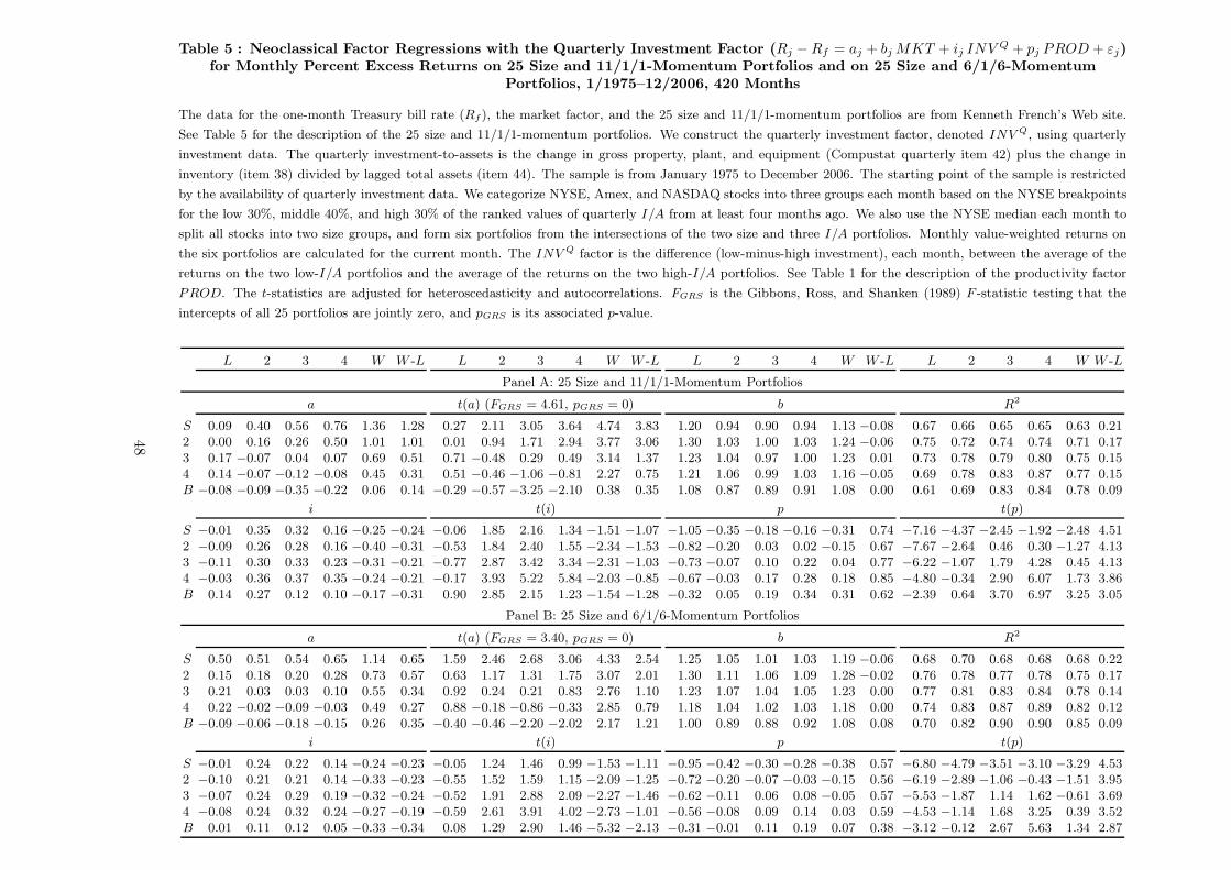
Table 5 : Neoclassical Factor Regressions with the Quarterly Investment Factor (Rj − Rf = aj + bj MKT + ij INV Q + pj PROD + εj)for Monthly Percent Excess Returns on 25 Size and 11/1/1-Momentum Portfolios and on 25 Size and 6/1/6-Momentum

Portfolios, 1/1975–12/2006, 420 Months

The data for the one-month Treasury bill rate (Rf ), the market factor, and the 25 size and 11/1/1-momentum portfolios are from Kenneth French’s Web site.

See Table 5 for the description of the 25 size and 11/1/1-momentum portfolios. We construct the quarterly investment factor, denoted INV Q, using quarterly

investment data. The quarterly investment-to-assets is the change in gross property, plant, and equipment (Compustat quarterly item 42) plus the change in

inventory (item 38) divided by lagged total assets (item 44). The sample is from January 1975 to December 2006. The starting point of the sample is restricted

by the availability of quarterly investment data. We categorize NYSE, Amex, and NASDAQ stocks into three groups each month based on the NYSE breakpoints

for the low 30%, middle 40%, and high 30% of the ranked values of quarterly I/A from at least four months ago. We also use the NYSE median each month to

split all stocks into two size groups, and form six portfolios from the intersections of the two size and three I/A portfolios. Monthly value-weighted returns on

the six portfolios are calculated for the current month. The INV Q factor is the difference (low-minus-high investment), each month, between the average of the

returns on the two low-I/A portfolios and the average of the returns on the two high-I/A portfolios. See Table 1 for the description of the productivity factor

PROD. The t-statistics are adjusted for heteroscedasticity and autocorrelations. FGRS is the Gibbons, Ross, and Shanken (1989) F -statistic testing that the

intercepts of all 25 portfolios are jointly zero, and pGRS is its associated p-value.

L 2 3 4 W W -L L 2 3 4 W W -L L 2 3 4 W W -L L 2 3 4 W W -L

Panel A: 25 Size and 11/1/1-Momentum Portfolios

a t(a) (FGRS = 4.61, pGRS = 0) b R2

S 0.09 0.40 0.56 0.76 1.36 1.28 0.27 2.11 3.05 3.64 4.74 3.83 1.20 0.94 0.90 0.94 1.13 −0.08 0.67 0.66 0.65 0.65 0.63 0.212 0.00 0.16 0.26 0.50 1.01 1.01 0.01 0.94 1.71 2.94 3.77 3.06 1.30 1.03 1.00 1.03 1.24 −0.06 0.75 0.72 0.74 0.74 0.71 0.173 0.17 −0.07 0.04 0.07 0.69 0.51 0.71 −0.48 0.29 0.49 3.14 1.37 1.23 1.04 0.97 1.00 1.23 0.01 0.73 0.78 0.79 0.80 0.75 0.154 0.14 −0.07 −0.12 −0.08 0.45 0.31 0.51 −0.46 −1.06 −0.81 2.27 0.75 1.21 1.06 0.99 1.03 1.16 −0.05 0.69 0.78 0.83 0.87 0.77 0.15B −0.08 −0.09 −0.35 −0.22 0.06 0.14 −0.29 −0.57 −3.25 −2.10 0.38 0.35 1.08 0.87 0.89 0.91 1.08 0.00 0.61 0.69 0.83 0.84 0.78 0.09

i t(i) p t(p)

S −0.01 0.35 0.32 0.16 −0.25 −0.24 −0.06 1.85 2.16 1.34 −1.51 −1.07 −1.05 −0.35 −0.18 −0.16 −0.31 0.74 −7.16 −4.37 −2.45 −1.92 −2.48 4.512 −0.09 0.26 0.28 0.16 −0.40 −0.31 −0.53 1.84 2.40 1.55 −2.34 −1.53 −0.82 −0.20 0.03 0.02 −0.15 0.67 −7.67 −2.64 0.46 0.30 −1.27 4.133 −0.11 0.30 0.33 0.23 −0.31 −0.21 −0.77 2.87 3.42 3.34 −2.31 −1.03 −0.73 −0.07 0.10 0.22 0.04 0.77 −6.22 −1.07 1.79 4.28 0.45 4.134 −0.03 0.36 0.37 0.35 −0.24 −0.21 −0.17 3.93 5.22 5.84 −2.03 −0.85 −0.67 −0.03 0.17 0.28 0.18 0.85 −4.80 −0.34 2.90 6.07 1.73 3.86B 0.14 0.27 0.12 0.10 −0.17 −0.31 0.90 2.85 2.15 1.23 −1.54 −1.28 −0.32 0.05 0.19 0.34 0.31 0.62 −2.39 0.64 3.70 6.97 3.25 3.05

Panel B: 25 Size and 6/1/6-Momentum Portfolios

a t(a) (FGRS = 3.40, pGRS = 0) b R2

S 0.50 0.51 0.54 0.65 1.14 0.65 1.59 2.46 2.68 3.06 4.33 2.54 1.25 1.05 1.01 1.03 1.19 −0.06 0.68 0.70 0.68 0.68 0.68 0.222 0.15 0.18 0.20 0.28 0.73 0.57 0.63 1.17 1.31 1.75 3.07 2.01 1.30 1.11 1.06 1.09 1.28 −0.02 0.76 0.78 0.77 0.78 0.75 0.173 0.21 0.03 0.03 0.10 0.55 0.34 0.92 0.24 0.21 0.83 2.76 1.10 1.23 1.07 1.04 1.05 1.23 0.00 0.77 0.81 0.83 0.84 0.78 0.144 0.22 −0.02 −0.09 −0.03 0.49 0.27 0.88 −0.18 −0.86 −0.33 2.85 0.79 1.18 1.04 1.02 1.03 1.18 0.00 0.74 0.83 0.87 0.89 0.82 0.12B −0.09 −0.06 −0.18 −0.15 0.26 0.35 −0.40 −0.46 −2.20 −2.02 2.17 1.21 1.00 0.89 0.88 0.92 1.08 0.08 0.70 0.82 0.90 0.90 0.85 0.09

i t(i) p t(p)

S −0.01 0.24 0.22 0.14 −0.24 −0.23 −0.05 1.24 1.46 0.99 −1.53 −1.11 −0.95 −0.42 −0.30 −0.28 −0.38 0.57 −6.80 −4.79 −3.51 −3.10 −3.29 4.532 −0.10 0.21 0.21 0.14 −0.33 −0.23 −0.55 1.52 1.59 1.15 −2.09 −1.25 −0.72 −0.20 −0.07 −0.03 −0.15 0.56 −6.19 −2.89 −1.06 −0.43 −1.51 3.953 −0.07 0.24 0.29 0.19 −0.32 −0.24 −0.52 1.91 2.88 2.09 −2.27 −1.46 −0.62 −0.11 0.06 0.08 −0.05 0.57 −5.53 −1.87 1.14 1.62 −0.61 3.694 −0.08 0.24 0.32 0.24 −0.27 −0.19 −0.59 2.61 3.91 4.02 −2.73 −1.01 −0.56 −0.08 0.09 0.14 0.03 0.59 −4.53 −1.14 1.68 3.25 0.39 3.52B 0.01 0.11 0.12 0.05 −0.33 −0.34 0.08 1.29 2.90 1.46 −5.32 −2.13 −0.31 −0.01 0.11 0.19 0.07 0.38 −3.12 −0.12 2.67 5.63 1.34 2.87

48

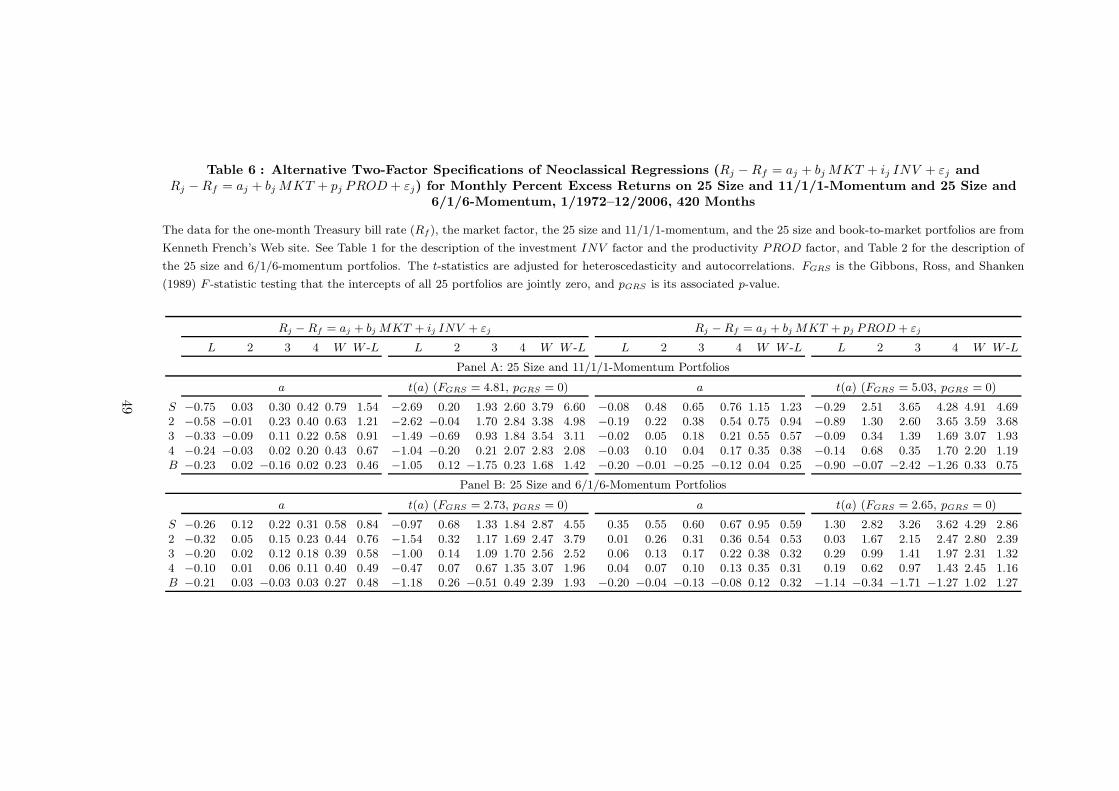
Table 6 : Alternative Two-Factor Specifications of Neoclassical Regressions (Rj − Rf = aj + bj MKT + ij INV + εj andRj − Rf = aj + bj MKT + pj PROD + εj) for Monthly Percent Excess Returns on 25 Size and 11/1/1-Momentum and 25 Size and

6/1/6-Momentum, 1/1972–12/2006, 420 Months

The data for the one-month Treasury bill rate (Rf ), the market factor, the 25 size and 11/1/1-momentum, and the 25 size and book-to-market portfolios are from

Kenneth French’s Web site. See Table 1 for the description of the investment INV factor and the productivity PROD factor, and Table 2 for the description of

the 25 size and 6/1/6-momentum portfolios. The t-statistics are adjusted for heteroscedasticity and autocorrelations. FGRS is the Gibbons, Ross, and Shanken

(1989) F -statistic testing that the intercepts of all 25 portfolios are jointly zero, and pGRS is its associated p-value.

Rj − Rf = aj + bj MKT + ij INV + εj Rj − Rf = aj + bj MKT + pj PROD + εj

L 2 3 4 W W -L L 2 3 4 W W -L L 2 3 4 W W -L L 2 3 4 W W -L

Panel A: 25 Size and 11/1/1-Momentum Portfolios

a t(a) (FGRS = 4.81, pGRS = 0) a t(a) (FGRS = 5.03, pGRS = 0)

S −0.75 0.03 0.30 0.42 0.79 1.54 −2.69 0.20 1.93 2.60 3.79 6.60 −0.08 0.48 0.65 0.76 1.15 1.23 −0.29 2.51 3.65 4.28 4.91 4.692 −0.58 −0.01 0.23 0.40 0.63 1.21 −2.62 −0.04 1.70 2.84 3.38 4.98 −0.19 0.22 0.38 0.54 0.75 0.94 −0.89 1.30 2.60 3.65 3.59 3.683 −0.33 −0.09 0.11 0.22 0.58 0.91 −1.49 −0.69 0.93 1.84 3.54 3.11 −0.02 0.05 0.18 0.21 0.55 0.57 −0.09 0.34 1.39 1.69 3.07 1.934 −0.24 −0.03 0.02 0.20 0.43 0.67 −1.04 −0.20 0.21 2.07 2.83 2.08 −0.03 0.10 0.04 0.17 0.35 0.38 −0.14 0.68 0.35 1.70 2.20 1.19B −0.23 0.02 −0.16 0.02 0.23 0.46 −1.05 0.12 −1.75 0.23 1.68 1.42 −0.20 −0.01 −0.25 −0.12 0.04 0.25 −0.90 −0.07 −2.42 −1.26 0.33 0.75

Panel B: 25 Size and 6/1/6-Momentum Portfolios

a t(a) (FGRS = 2.73, pGRS = 0) a t(a) (FGRS = 2.65, pGRS = 0)

S −0.26 0.12 0.22 0.31 0.58 0.84 −0.97 0.68 1.33 1.84 2.87 4.55 0.35 0.55 0.60 0.67 0.95 0.59 1.30 2.82 3.26 3.62 4.29 2.862 −0.32 0.05 0.15 0.23 0.44 0.76 −1.54 0.32 1.17 1.69 2.47 3.79 0.01 0.26 0.31 0.36 0.54 0.53 0.03 1.67 2.15 2.47 2.80 2.393 −0.20 0.02 0.12 0.18 0.39 0.58 −1.00 0.14 1.09 1.70 2.56 2.52 0.06 0.13 0.17 0.22 0.38 0.32 0.29 0.99 1.41 1.97 2.31 1.324 −0.10 0.01 0.06 0.11 0.40 0.49 −0.47 0.07 0.67 1.35 3.07 1.96 0.04 0.07 0.10 0.13 0.35 0.31 0.19 0.62 0.97 1.43 2.45 1.16B −0.21 0.03 −0.03 0.03 0.27 0.48 −1.18 0.26 −0.51 0.49 2.39 1.93 −0.20 −0.04 −0.13 −0.08 0.12 0.32 −1.14 −0.34 −1.71 −1.27 1.02 1.27

49

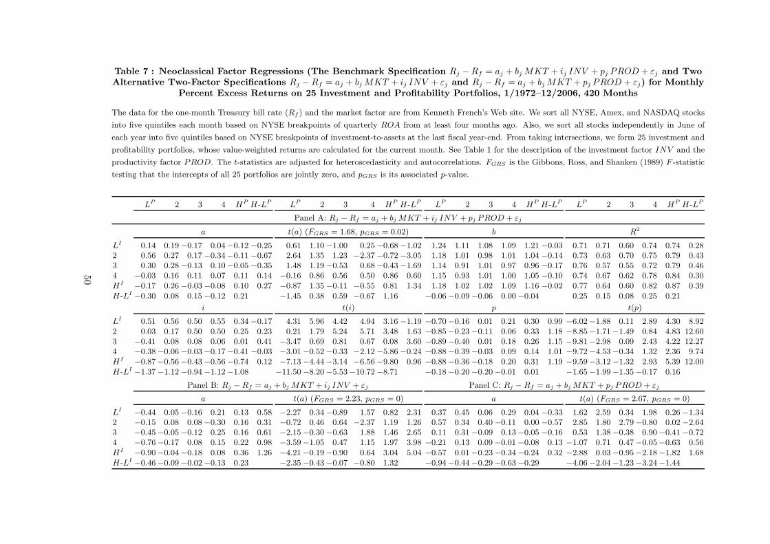
Table 7 : Neoclassical Factor Regressions (The Benchmark Specification Rj − Rf = aj + bj MKT + ij INV + pj PROD + εj and TwoAlternative Two-Factor Specifications Rj − Rf = aj + bj MKT + ij INV + εj and Rj − Rf = aj + bj MKT + pj PROD + εj) for Monthly

Percent Excess Returns on 25 Investment and Profitability Portfolios, 1/1972–12/2006, 420 Months

The data for the one-month Treasury bill rate (Rf ) and the market factor are from Kenneth French’s Web site. We sort all NYSE, Amex, and NASDAQ stocks

into five quintiles each month based on NYSE breakpoints of quarterly ROA from at least four months ago. Also, we sort all stocks independently in June of

each year into five quintiles based on NYSE breakpoints of investment-to-assets at the last fiscal year-end. From taking intersections, we form 25 investment and

profitability portfolios, whose value-weighted returns are calculated for the current month. See Table 1 for the description of the investment factor INV and the

productivity factor PROD. The t-statistics are adjusted for heteroscedasticity and autocorrelations. FGRS is the Gibbons, Ross, and Shanken (1989) F -statistic

testing that the intercepts of all 25 portfolios are jointly zero, and pGRS is its associated p-value.

LP 2 3 4 HP H-LP LP 2 3 4 HP H-LP LP 2 3 4 HP H-LP LP 2 3 4 HP H-LP

Panel A: Rj − Rf = aj + bj MKT + ij INV + pj PROD + εj

a t(a) (FGRS = 1.68, pGRS = 0.02) b R2

LI 0.14 0.19 −0.17 0.04−0.12 −0.25 0.61 1.10 −1.00 0.25 −0.68 −1.02 1.24 1.11 1.08 1.09 1.21 −0.03 0.71 0.71 0.60 0.74 0.74 0.282 0.56 0.27 0.17 −0.34−0.11 −0.67 2.64 1.35 1.23 −2.37 −0.72 −3.05 1.18 1.01 0.98 1.01 1.04 −0.14 0.73 0.63 0.70 0.75 0.79 0.433 0.30 0.28 −0.13 0.10−0.05 −0.35 1.48 1.19 −0.53 0.68 −0.43 −1.69 1.14 0.91 1.01 0.97 0.96 −0.17 0.76 0.57 0.55 0.72 0.79 0.464 −0.03 0.16 0.11 0.07 0.11 0.14 −0.16 0.86 0.56 0.50 0.86 0.60 1.15 0.93 1.01 1.00 1.05 −0.10 0.74 0.67 0.62 0.78 0.84 0.30HI

−0.17 0.26 −0.03−0.08 0.10 0.27 −0.87 1.35 −0.11 −0.55 0.81 1.34 1.18 1.02 1.02 1.09 1.16 −0.02 0.77 0.64 0.60 0.82 0.87 0.39H-LI

−0.30 0.08 0.15 −0.12 0.21 −1.45 0.38 0.59 −0.67 1.16 −0.06−0.09 −0.06 0.00−0.04 0.25 0.15 0.08 0.25 0.21

i t(i) p t(p)

LI 0.51 0.56 0.50 0.55 0.34 −0.17 4.31 5.96 4.42 4.94 3.16 −1.19 −0.70−0.16 0.01 0.21 0.30 0.99 −6.02−1.88 0.11 2.89 4.30 8.922 0.03 0.17 0.50 0.50 0.25 0.23 0.21 1.79 5.24 5.71 3.48 1.63 −0.85−0.23 −0.11 0.06 0.33 1.18 −8.85−1.71−1.49 0.84 4.83 12.603 −0.41 0.08 0.08 0.06 0.01 0.41 −3.47 0.69 0.81 0.67 0.08 3.60 −0.89−0.40 0.01 0.18 0.26 1.15 −9.81−2.98 0.09 2.43 4.22 12.274 −0.38−0.06 −0.03−0.17−0.41 −0.03 −3.01−0.52 −0.33 −2.12 −5.86 −0.24 −0.88−0.39 −0.03 0.09 0.14 1.01 −9.72−4.53−0.34 1.32 2.36 9.74HI

−0.87−0.56 −0.43−0.56−0.74 0.12 −7.13−4.44 −3.14 −6.56 −9.80 0.96 −0.88−0.36 −0.18 0.20 0.31 1.19 −9.59−3.12−1.32 2.93 5.39 12.00H-LI

−1.37−1.12 −0.94−1.12−1.08 −11.50−8.20 −5.53−10.72 −8.71 −0.18−0.20 −0.20−0.01 0.01 −1.65−1.99−1.35 −0.17 0.16

Panel B: Rj − Rf = aj + bj MKT + ij INV + εj Panel C: Rj − Rf = aj + bj MKT + pj PROD + εj

a t(a) (FGRS = 2.23, pGRS = 0) a t(a) (FGRS = 2.67, pGRS = 0)

LI−0.44 0.05 −0.16 0.21 0.13 0.58 −2.27 0.34 −0.89 1.57 0.82 2.31 0.37 0.45 0.06 0.29 0.04 −0.33 1.62 2.59 0.34 1.98 0.26 −1.34

2 −0.15 0.08 0.08 −0.30 0.16 0.31 −0.72 0.46 0.64 −2.37 1.19 1.26 0.57 0.34 0.40 −0.11 0.00 −0.57 2.85 1.80 2.79 −0.80 0.02 −2.643 −0.45−0.05 −0.12 0.25 0.16 0.61 −2.15−0.30 −0.63 1.88 1.46 2.65 0.11 0.31 −0.09 0.13−0.05 −0.16 0.53 1.38−0.38 0.90 −0.41 −0.724 −0.76−0.17 0.08 0.15 0.22 0.98 −3.59−1.05 0.47 1.15 1.97 3.98 −0.21 0.13 0.09 −0.01−0.08 0.13 −1.07 0.71 0.47 −0.05−0.63 0.56HI

−0.90−0.04 −0.18 0.08 0.36 1.26 −4.21−0.19 −0.90 0.64 3.04 5.04 −0.57 0.01 −0.23−0.34−0.24 0.32 −2.88 0.03−0.95 −2.18−1.82 1.68H-LI

−0.46−0.09 −0.02−0.13 0.23 −2.35−0.43 −0.07 −0.80 1.32 −0.94−0.44 −0.29−0.63−0.29 −4.06−2.04−1.23 −3.24−1.44

50

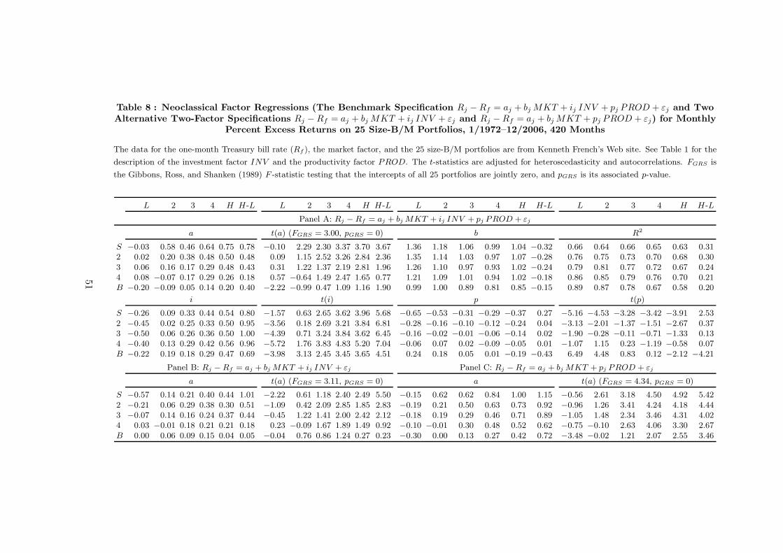
Table 8 : Neoclassical Factor Regressions (The Benchmark Specification Rj − Rf = aj + bj MKT + ij INV + pj PROD + εj and TwoAlternative Two-Factor Specifications Rj − Rf = aj + bj MKT + ij INV + εj and Rj − Rf = aj + bj MKT + pj PROD + εj) for Monthly

Percent Excess Returns on 25 Size-B/M Portfolios, 1/1972–12/2006, 420 Months

The data for the one-month Treasury bill rate (Rf ), the market factor, and the 25 size-B/M portfolios are from Kenneth French’s Web site. See Table 1 for the

description of the investment factor INV and the productivity factor PROD. The t-statistics are adjusted for heteroscedasticity and autocorrelations. FGRS is

the Gibbons, Ross, and Shanken (1989) F -statistic testing that the intercepts of all 25 portfolios are jointly zero, and pGRS is its associated p-value.

L 2 3 4 H H-L L 2 3 4 H H-L L 2 3 4 H H-L L 2 3 4 H H-L

Panel A: Rj − Rf = aj + bj MKT + ij INV + pj PROD + εj

a t(a) (FGRS = 3.00, pGRS = 0) b R2

S −0.03 0.58 0.46 0.64 0.75 0.78 −0.10 2.29 2.30 3.37 3.70 3.67 1.36 1.18 1.06 0.99 1.04 −0.32 0.66 0.64 0.66 0.65 0.63 0.312 0.02 0.20 0.38 0.48 0.50 0.48 0.09 1.15 2.52 3.26 2.84 2.36 1.35 1.14 1.03 0.97 1.07 −0.28 0.76 0.75 0.73 0.70 0.68 0.303 0.06 0.16 0.17 0.29 0.48 0.43 0.31 1.22 1.37 2.19 2.81 1.96 1.26 1.10 0.97 0.93 1.02 −0.24 0.79 0.81 0.77 0.72 0.67 0.244 0.08 −0.07 0.17 0.29 0.26 0.18 0.57 −0.64 1.49 2.47 1.65 0.77 1.21 1.09 1.01 0.94 1.02 −0.18 0.86 0.85 0.79 0.76 0.70 0.21B −0.20 −0.09 0.05 0.14 0.20 0.40 −2.22 −0.99 0.47 1.09 1.16 1.90 0.99 1.00 0.89 0.81 0.85 −0.15 0.89 0.87 0.78 0.67 0.58 0.20

i t(i) p t(p)

S −0.26 0.09 0.33 0.44 0.54 0.80 −1.57 0.63 2.65 3.62 3.96 5.68 −0.65 −0.53 −0.31 −0.29 −0.37 0.27 −5.16 −4.53 −3.28 −3.42 −3.91 2.532 −0.45 0.02 0.25 0.33 0.50 0.95 −3.56 0.18 2.69 3.21 3.84 6.81 −0.28 −0.16 −0.10 −0.12 −0.24 0.04 −3.13 −2.01 −1.37 −1.51 −2.67 0.373 −0.50 0.06 0.26 0.36 0.50 1.00 −4.39 0.71 3.24 3.84 3.62 6.45 −0.16 −0.02 −0.01 −0.06 −0.14 0.02 −1.90 −0.28 −0.11 −0.71 −1.33 0.134 −0.40 0.13 0.29 0.42 0.56 0.96 −5.72 1.76 3.83 4.83 5.20 7.04 −0.06 0.07 0.02 −0.09 −0.05 0.01 −1.07 1.15 0.23 −1.19 −0.58 0.07B −0.22 0.19 0.18 0.29 0.47 0.69 −3.98 3.13 2.45 3.45 3.65 4.51 0.24 0.18 0.05 0.01 −0.19 −0.43 6.49 4.48 0.83 0.12 −2.12 −4.21

Panel B: Rj − Rf = aj + bj MKT + ij INV + εj Panel C: Rj − Rf = aj + bj MKT + pj PROD + εj

a t(a) (FGRS = 3.11, pGRS = 0) a t(a) (FGRS = 4.34, pGRS = 0)

S −0.57 0.14 0.21 0.40 0.44 1.01 −2.22 0.61 1.18 2.40 2.49 5.50 −0.15 0.62 0.62 0.84 1.00 1.15 −0.56 2.61 3.18 4.50 4.92 5.422 −0.21 0.06 0.29 0.38 0.30 0.51 −1.09 0.42 2.09 2.85 1.85 2.83 −0.19 0.21 0.50 0.63 0.73 0.92 −0.96 1.26 3.41 4.24 4.18 4.443 −0.07 0.14 0.16 0.24 0.37 0.44 −0.45 1.22 1.41 2.00 2.42 2.12 −0.18 0.19 0.29 0.46 0.71 0.89 −1.05 1.48 2.34 3.46 4.31 4.024 0.03 −0.01 0.18 0.21 0.21 0.18 0.23 −0.09 1.67 1.89 1.49 0.92 −0.10 −0.01 0.30 0.48 0.52 0.62 −0.75 −0.10 2.63 4.06 3.30 2.67B 0.00 0.06 0.09 0.15 0.04 0.05 −0.04 0.76 0.86 1.24 0.27 0.23 −0.30 0.00 0.13 0.27 0.42 0.72 −3.48 −0.02 1.21 2.07 2.55 3.46

51

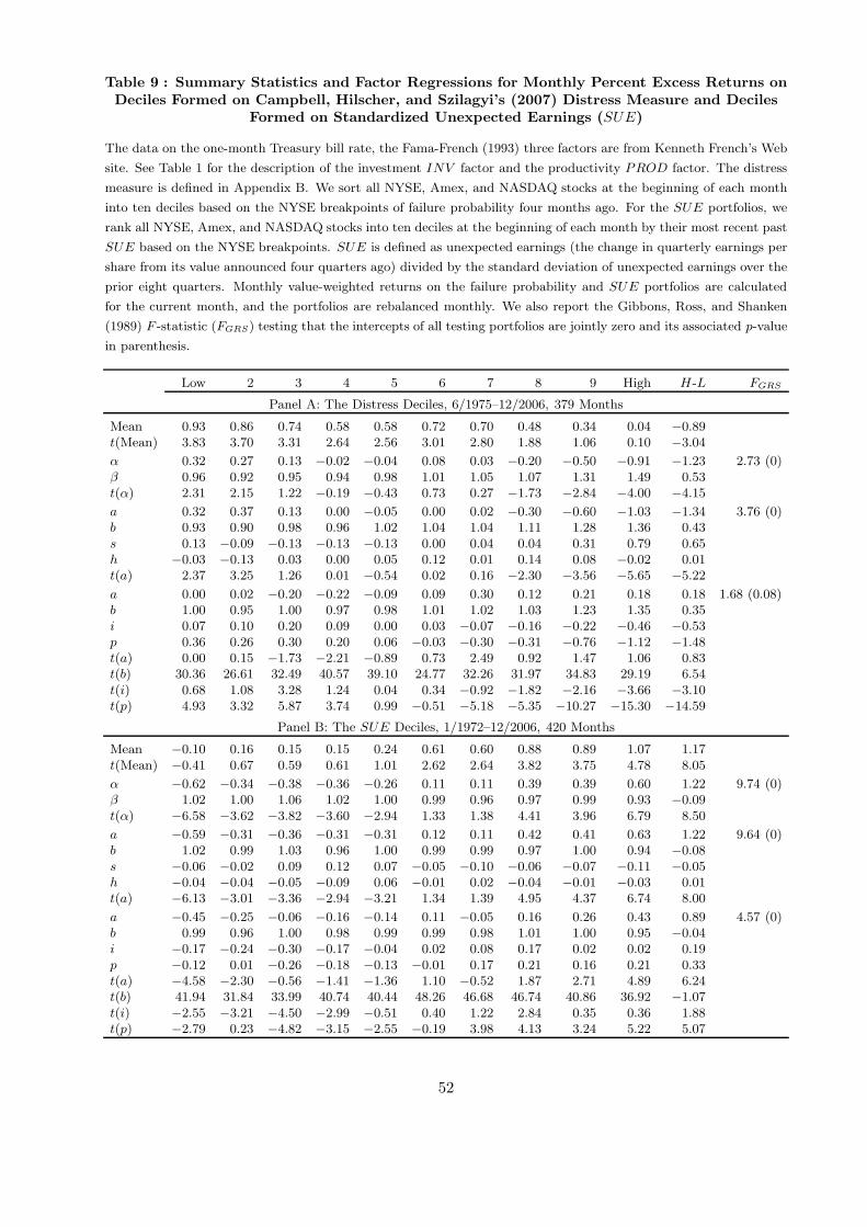
Table 9 : Summary Statistics and Factor Regressions for Monthly Percent Excess Returns onDeciles Formed on Campbell, Hilscher, and Szilagyi’s (2007) Distress Measure and Deciles

Formed on Standardized Unexpected Earnings (SUE)

The data on the one-month Treasury bill rate, the Fama-French (1993) three factors are from Kenneth French’s Web

site. See Table 1 for the description of the investment INV factor and the productivity PROD factor. The distress

measure is defined in Appendix B. We sort all NYSE, Amex, and NASDAQ stocks at the beginning of each month

into ten deciles based on the NYSE breakpoints of failure probability four months ago. For the SUE portfolios, we

rank all NYSE, Amex, and NASDAQ stocks into ten deciles at the beginning of each month by their most recent past

SUE based on the NYSE breakpoints. SUE is defined as unexpected earnings (the change in quarterly earnings per

share from its value announced four quarters ago) divided by the standard deviation of unexpected earnings over the

prior eight quarters. Monthly value-weighted returns on the failure probability and SUE portfolios are calculated

for the current month, and the portfolios are rebalanced monthly. We also report the Gibbons, Ross, and Shanken

(1989) F -statistic (FGRS) testing that the intercepts of all testing portfolios are jointly zero and its associated p-value

in parenthesis.

Low 2 3 4 5 6 7 8 9 High H-L FGRS

Panel A: The Distress Deciles, 6/1975–12/2006, 379 Months

Mean 0.93 0.86 0.74 0.58 0.58 0.72 0.70 0.48 0.34 0.04 −0.89t(Mean) 3.83 3.70 3.31 2.64 2.56 3.01 2.80 1.88 1.06 0.10 −3.04

α 0.32 0.27 0.13 −0.02 −0.04 0.08 0.03 −0.20 −0.50 −0.91 −1.23 2.73 (0)β 0.96 0.92 0.95 0.94 0.98 1.01 1.05 1.07 1.31 1.49 0.53t(α) 2.31 2.15 1.22 −0.19 −0.43 0.73 0.27 −1.73 −2.84 −4.00 −4.15

a 0.32 0.37 0.13 0.00 −0.05 0.00 0.02 −0.30 −0.60 −1.03 −1.34 3.76 (0)b 0.93 0.90 0.98 0.96 1.02 1.04 1.04 1.11 1.28 1.36 0.43s 0.13 −0.09 −0.13 −0.13 −0.13 0.00 0.04 0.04 0.31 0.79 0.65h −0.03 −0.13 0.03 0.00 0.05 0.12 0.01 0.14 0.08 −0.02 0.01t(a) 2.37 3.25 1.26 0.01 −0.54 0.02 0.16 −2.30 −3.56 −5.65 −5.22

a 0.00 0.02 −0.20 −0.22 −0.09 0.09 0.30 0.12 0.21 0.18 0.18 1.68 (0.08)b 1.00 0.95 1.00 0.97 0.98 1.01 1.02 1.03 1.23 1.35 0.35i 0.07 0.10 0.20 0.09 0.00 0.03 −0.07 −0.16 −0.22 −0.46 −0.53p 0.36 0.26 0.30 0.20 0.06 −0.03 −0.30 −0.31 −0.76 −1.12 −1.48t(a) 0.00 0.15 −1.73 −2.21 −0.89 0.73 2.49 0.92 1.47 1.06 0.83t(b) 30.36 26.61 32.49 40.57 39.10 24.77 32.26 31.97 34.83 29.19 6.54t(i) 0.68 1.08 3.28 1.24 0.04 0.34 −0.92 −1.82 −2.16 −3.66 −3.10t(p) 4.93 3.32 5.87 3.74 0.99 −0.51 −5.18 −5.35 −10.27 −15.30 −14.59

Panel B: The SUE Deciles, 1/1972–12/2006, 420 Months

Mean −0.10 0.16 0.15 0.15 0.24 0.61 0.60 0.88 0.89 1.07 1.17t(Mean) −0.41 0.67 0.59 0.61 1.01 2.62 2.64 3.82 3.75 4.78 8.05

α −0.62 −0.34 −0.38 −0.36 −0.26 0.11 0.11 0.39 0.39 0.60 1.22 9.74 (0)β 1.02 1.00 1.06 1.02 1.00 0.99 0.96 0.97 0.99 0.93 −0.09t(α) −6.58 −3.62 −3.82 −3.60 −2.94 1.33 1.38 4.41 3.96 6.79 8.50

a −0.59 −0.31 −0.36 −0.31 −0.31 0.12 0.11 0.42 0.41 0.63 1.22 9.64 (0)b 1.02 0.99 1.03 0.96 1.00 0.99 0.99 0.97 1.00 0.94 −0.08s −0.06 −0.02 0.09 0.12 0.07 −0.05 −0.10 −0.06 −0.07 −0.11 −0.05h −0.04 −0.04 −0.05 −0.09 0.06 −0.01 0.02 −0.04 −0.01 −0.03 0.01t(a) −6.13 −3.01 −3.36 −2.94 −3.21 1.34 1.39 4.95 4.37 6.74 8.00

a −0.45 −0.25 −0.06 −0.16 −0.14 0.11 −0.05 0.16 0.26 0.43 0.89 4.57 (0)b 0.99 0.96 1.00 0.98 0.99 0.99 0.98 1.01 1.00 0.95 −0.04i −0.17 −0.24 −0.30 −0.17 −0.04 0.02 0.08 0.17 0.02 0.02 0.19p −0.12 0.01 −0.26 −0.18 −0.13 −0.01 0.17 0.21 0.16 0.21 0.33t(a) −4.58 −2.30 −0.56 −1.41 −1.36 1.10 −0.52 1.87 2.71 4.89 6.24t(b) 41.94 31.84 33.99 40.74 40.44 48.26 46.68 46.74 40.86 36.92 −1.07t(i) −2.55 −3.21 −4.50 −2.99 −0.51 0.40 1.22 2.84 0.35 0.36 1.88t(p) −2.79 0.23 −4.82 −3.15 −2.55 −0.19 3.98 4.13 3.24 5.22 5.07

52

Table 10 : Summary Statistics and Factor Regressions for Monthly Percent Excess Returnson Ten Accruals Deciles and Ten Net Stock Issues Deciles, 1/1972–12/2006, 420 Months

The data on the one-month Treasury bill rate, the Fama-French (1993) three factors are from Kenneth French’s Web

site. See the caption of Table 1 for the description of the investment INV factor and the productivity PROD factor.

Accruals are measured as the change of operating working capital per split-adjusted share from year t−1 to t divided

by book equity per split-adjusted share at t. Operating working capital is current assets (Compustat annual item 4)

minus cash and short term investment (item 1) minus current liabilities (item 5) plus debt in current liabilities (item

34). We measure net stock issues as the the natural log of the ratio of the split-adjusted shares outstanding at the

fiscal yearend in t−1 (item 25 times the Compustat adjustment factor, item 27) divided by the split-adjusted shares

outstanding at the fiscal yearend in t−2. In June of each year t, we sort all NYSE, Amex, and NASDAQ stocks

into ten deciles based on the NYSE breakpoints of accruals and net stock issues measured at the end of last fiscal

yearend. Monthly value-weighted returns are calculated from July of year t to June of year t + 1. We also report the

Gibbons, Ross, and Shanken (1989) F -statistic (FGRS) testing that the intercepts of all testing portfolios are jointly

zero and its associated p-value in parenthesis.

Low 2 3 4 5 6 7 8 9 High H-L FGRS

Panel A: The Accrual Deciles

Mean 0.73 0.61 0.50 0.53 0.57 0.56 0.53 0.53 0.47 0.22 −0.52t(Mean) 2.59 2.35 2.14 2.44 2.68 2.51 2.23 2.11 1.74 0.74 −4.13

α 0.14 0.05 0.00 0.05 0.11 0.07 0.01 −0.02 −0.11 −0.41 −0.55 3.00 (0)β 1.17 1.11 1.01 0.94 0.90 0.97 1.03 1.08 1.15 1.25 0.07t(α) 1.27 0.61 −0.06 0.78 1.47 1.11 0.15 −0.19 −1.17 −3.46 −4.41

a 0.10 0.14 0.01 0.00 0.05 0.02 −0.02 −0.03 −0.10 −0.47 −0.57 3.22 (0)b 1.12 1.06 1.01 0.98 0.95 1.01 1.05 1.07 1.11 1.19 0.07s 0.29 0.07 −0.06 −0.06 −0.05 −0.07 −0.01 0.10 0.14 0.33 0.04h 0.02 −0.14 −0.01 0.09 0.11 0.09 0.05 0.01 −0.03 0.04 0.02t(a) 0.91 1.62 0.11 0.03 0.55 0.26 −0.28 −0.34 −1.06 −3.95 −4.35

a 0.17 0.22 0.13 0.14 0.22 0.13 0.08 0.14 0.09 −0.21 −0.38 2.96 (0)b 1.18 1.08 0.98 0.93 0.88 0.95 1.01 1.03 1.08 1.17 0.00i 0.05 −0.16 −0.14 −0.05 −0.14 −0.09 −0.14 −0.32 −0.41 −0.47 −0.51p −0.06 −0.13 −0.11 −0.09 −0.06 −0.02 −0.01 −0.03 −0.03 −0.01 0.06t(a) 1.24 2.15 1.61 1.79 2.34 1.68 1.06 1.44 0.80 −1.57 −2.97t(b) 39.51 53.32 46.24 44.23 42.49 49.00 51.84 49.60 38.13 38.41 −0.14t(i) 0.51 −2.37 −2.38 −1.02 −2.04 −1.84 −2.52 −4.17 −5.95 −5.10 −5.33t(p) −1.20 −2.77 −2.51 −2.14 −1.38 −0.49 −0.27 −0.56 −0.63 −0.13 0.96

Panel B: The Net Stock Issues Deciles

Mean 1.00 0.82 0.77 0.57 0.27 0.70 0.72 0.78 0.24 0.04 −0.96t(Mean) 4.36 3.65 3.34 2.45 1.01 2.99 2.94 2.95 0.81 0.13 −5.23

α 0.54 0.37 0.32 0.11 −0.28 0.21 0.20 0.22 −0.36 −0.57 −1.11 3.97 (0)β 0.91 0.89 0.88 0.90 1.07 0.96 1.02 1.10 1.18 1.20 0.29t(α) 4.02 2.72 2.16 0.69 −1.82 1.85 2.03 2.08 −2.11 −3.73 −4.68

a 0.32 0.24 0.24 −0.02 −0.19 0.13 0.17 0.22 −0.27 −0.51 −0.83 3.18 (0)b 1.06 1.00 0.94 0.98 1.03 1.02 1.04 1.08 1.10 1.12 0.06s 0.05 −0.08 −0.01 0.05 −0.05 −0.01 0.01 0.10 0.08 0.17 0.12h 0.40 0.26 0.15 0.23 −0.15 0.15 0.06 0.00 −0.17 −0.13 −0.53t(a) 2.94 1.91 1.60 −0.13 −1.41 1.18 1.67 1.97 −1.57 −3.32 −4.01

a 0.25 0.12 0.15 −0.06 0.07 0.05 0.20 0.41 0.27 −0.04 −0.29 2.26 (0.02)b 0.98 0.94 0.92 0.95 0.99 0.97 1.00 1.04 1.02 1.06 0.09i 0.24 0.14 0.15 0.18 −0.31 0.00 −0.14 −0.27 −0.64 −0.52 −0.75p 0.21 0.20 0.12 0.11 −0.24 0.16 0.05 −0.10 −0.42 −0.36 −0.57t(a) 1.86 0.91 0.87 −0.46 0.52 0.45 1.80 3.44 1.75 −0.27 −1.31t(b) 35.55 32.41 23.46 23.27 29.09 35.74 38.81 37.30 27.53 35.66 1.95t(i) 2.50 1.32 1.84 2.36 −3.35 −0.03 −2.05 −3.39 −5.36 −5.25 −4.97t(p) 3.11 2.67 1.82 1.32 −3.78 2.77 1.18 −1.88 −7.43 −6.90 −6.69

53

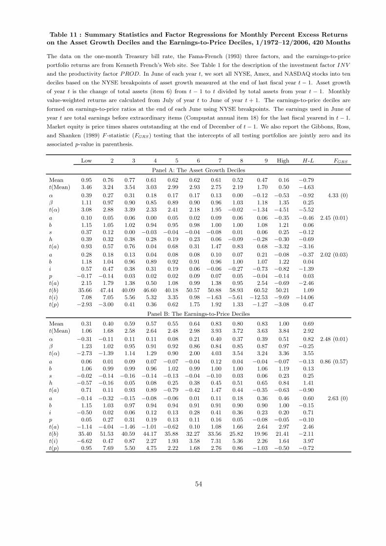
Table 11 : Summary Statistics and Factor Regressions for Monthly Percent Excess Returnson the Asset Growth Deciles and the Earnings-to-Price Deciles, 1/1972–12/2006, 420 Months

The data on the one-month Treasury bill rate, the Fama-French (1993) three factors, and the earnings-to-price

portfolio returns are from Kenneth French’s Web site. See Table 1 for the description of the investment factor INV

and the productivity factor PROD. In June of each year t, we sort all NYSE, Amex, and NASDAQ stocks into ten

deciles based on the NYSE breakpoints of asset growth measured at the end of last fiscal year t − 1. Asset growth

of year t is the change of total assets (item 6) from t − 1 to t divided by total assets from year t − 1. Monthly

value-weighted returns are calculated from July of year t to June of year t + 1. The earnings-to-price deciles are

formed on earnings-to-price ratios at the end of each June using NYSE breakpoints. The earnings used in June of

year t are total earnings before extraordinary items (Compustat annual item 18) for the last fiscal yearend in t − 1.

Market equity is price times shares outstanding at the end of December of t − 1. We also report the Gibbons, Ross,

and Shanken (1989) F -statistic (FGRS) testing that the intercepts of all testing portfolios are jointly zero and its

associated p-value in parenthesis.

Low 2 3 4 5 6 7 8 9 High H-L FGRS

Panel A: The Asset Growth Deciles

Mean 0.95 0.76 0.77 0.61 0.62 0.62 0.61 0.52 0.47 0.16 −0.79t(Mean) 3.46 3.24 3.54 3.03 2.99 2.93 2.75 2.19 1.70 0.50 −4.63

α 0.39 0.27 0.31 0.18 0.17 0.17 0.13 0.00 −0.12 −0.53 −0.92 4.33 (0)β 1.11 0.97 0.90 0.85 0.89 0.90 0.96 1.03 1.18 1.35 0.25t(α) 3.08 2.88 3.39 2.33 2.41 2.18 1.95 −0.02 −1.34 −4.51 −5.52

a 0.10 0.05 0.06 0.00 0.05 0.02 0.09 0.06 0.06 −0.35 −0.46 2.45 (0.01)b 1.15 1.05 1.02 0.94 0.95 0.98 1.00 1.00 1.08 1.21 0.06s 0.37 0.12 0.00 −0.03 −0.04 −0.04 −0.08 0.01 0.06 0.25 −0.12h 0.39 0.32 0.38 0.28 0.19 0.23 0.06 −0.09 −0.28 −0.30 −0.69t(a) 0.93 0.57 0.76 0.04 0.68 0.31 1.47 0.83 0.68 −3.32 −3.16

a 0.28 0.18 0.13 0.04 0.08 0.08 0.10 0.07 0.21 −0.08 −0.37 2.02 (0.03)b 1.18 1.04 0.96 0.89 0.92 0.91 0.96 1.00 1.07 1.22 0.04i 0.57 0.47 0.38 0.31 0.19 0.06 −0.06 −0.27 −0.73 −0.82 −1.39p −0.17 −0.14 0.03 0.02 0.02 0.09 0.07 0.05 −0.04 −0.14 0.03t(a) 2.15 1.79 1.38 0.50 1.08 0.99 1.38 0.95 2.54 −0.69 −2.46t(b) 35.66 47.44 40.09 46.60 40.18 50.57 50.88 58.93 60.52 50.21 1.09t(i) 7.08 7.05 5.56 5.32 3.35 0.98 −1.63 −5.61 −12.53 −9.69 −14.06t(p) −2.93 −3.00 0.41 0.36 0.62 1.75 1.92 1.33 −1.27 −3.08 0.47

Panel B: The Earnings-to-Price Deciles

Mean 0.31 0.40 0.59 0.57 0.55 0.64 0.83 0.80 0.83 1.00 0.69t(Mean) 1.06 1.68 2.58 2.64 2.48 2.98 3.93 3.72 3.63 3.84 2.92

α −0.31 −0.11 0.11 0.11 0.08 0.21 0.40 0.37 0.39 0.51 0.82 2.48 (0.01)β 1.23 1.02 0.95 0.91 0.92 0.86 0.84 0.85 0.87 0.97 −0.25t(α) −2.73 −1.39 1.14 1.29 0.90 2.00 4.03 3.54 3.24 3.36 3.55

a 0.06 0.01 0.09 0.07 −0.07 −0.04 0.12 0.04 −0.04 −0.07 −0.13 0.86 (0.57)b 1.06 0.99 0.99 0.96 1.02 0.99 1.00 1.00 1.06 1.19 0.13s −0.02 −0.14 −0.16 −0.14 −0.13 −0.04 −0.10 0.03 0.06 0.23 0.25h −0.57 −0.16 0.05 0.08 0.25 0.38 0.45 0.51 0.65 0.84 1.41t(a) 0.71 0.11 0.93 0.89 −0.79 −0.42 1.47 0.44 −0.35 −0.63 −0.90

a −0.14 −0.32 −0.15 −0.08 −0.06 0.01 0.11 0.18 0.36 0.46 0.60 2.63 (0)b 1.15 1.03 0.97 0.94 0.94 0.91 0.91 0.90 0.90 1.00 −0.15i −0.50 0.02 0.06 0.12 0.13 0.28 0.41 0.36 0.23 0.20 0.71p 0.05 0.27 0.31 0.19 0.13 0.11 0.16 0.05 −0.08 −0.05 −0.10t(a) −1.14 −4.04 −1.46 −1.01 −0.62 0.10 1.08 1.66 2.64 2.97 2.46t(b) 35.40 51.53 40.59 44.17 35.88 32.27 33.56 25.82 19.96 21.41 −2.11t(i) −6.62 0.47 0.87 2.27 1.93 3.58 7.31 5.36 2.26 1.64 3.97t(p) 0.95 7.69 5.50 4.75 2.22 1.68 2.76 0.86 −1.03 −0.50 −0.72

54

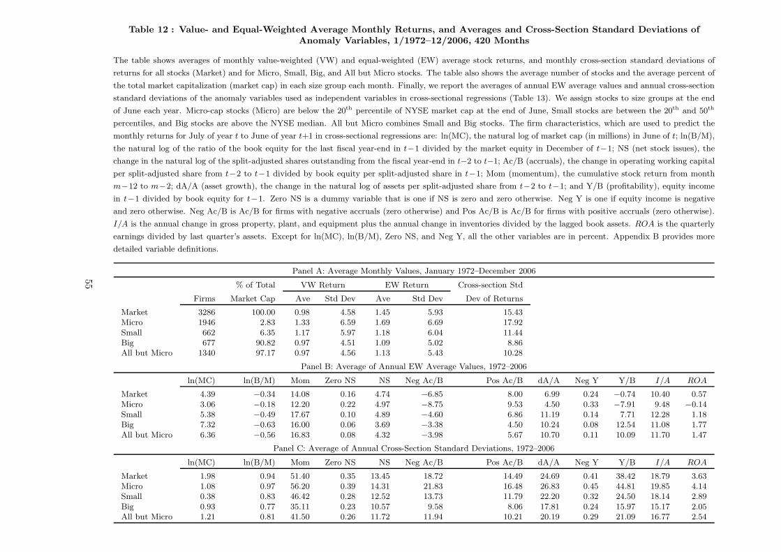
Table 12 : Value- and Equal-Weighted Average Monthly Returns, and Averages and Cross-Section Standard Deviations ofAnomaly Variables, 1/1972–12/2006, 420 Months

The table shows averages of monthly value-weighted (VW) and equal-weighted (EW) average stock returns, and monthly cross-section standard deviations of

returns for all stocks (Market) and for Micro, Small, Big, and All but Micro stocks. The table also shows the average number of stocks and the average percent of

the total market capitalization (market cap) in each size group each month. Finally, we report the averages of annual EW average values and annual cross-section

standard deviations of the anomaly variables used as independent variables in cross-sectional regressions (Table 13). We assign stocks to size groups at the end

of June each year. Micro-cap stocks (Micro) are below the 20th percentile of NYSE market cap at the end of June, Small stocks are between the 20th and 50th

percentiles, and Big stocks are above the NYSE median. All but Micro combines Small and Big stocks. The firm characteristics, which are used to predict the

monthly returns for July of year t to June of year t+1 in cross-sectional regressions are: ln(MC), the natural log of market cap (in millions) in June of t; ln(B/M),

the natural log of the ratio of the book equity for the last fiscal year-end in t−1 divided by the market equity in December of t−1; NS (net stock issues), the

change in the natural log of the split-adjusted shares outstanding from the fiscal year-end in t−2 to t−1; Ac/B (accruals), the change in operating working capital

per split-adjusted share from t−2 to t−1 divided by book equity per split-adjusted share in t−1; Mom (momentum), the cumulative stock return from month

m−12 to m−2; dA/A (asset growth), the change in the natural log of assets per split-adjusted share from t−2 to t−1; and Y/B (profitability), equity income

in t−1 divided by book equity for t−1. Zero NS is a dummy variable that is one if NS is zero and zero otherwise. Neg Y is one if equity income is negative

and zero otherwise. Neg Ac/B is Ac/B for firms with negative accruals (zero otherwise) and Pos Ac/B is Ac/B for firms with positive accruals (zero otherwise).

I/A is the annual change in gross property, plant, and equipment plus the annual change in inventories divided by the lagged book assets. ROA is the quarterly

earnings divided by last quarter’s assets. Except for ln(MC), ln(B/M), Zero NS, and Neg Y, all the other variables are in percent. Appendix B provides more

detailed variable definitions.

Panel A: Average Monthly Values, January 1972–December 2006

% of Total VW Return EW Return Cross-section Std

Firms Market Cap Ave Std Dev Ave Std Dev Dev of Returns

Market 3286 100.00 0.98 4.58 1.45 5.93 15.43Micro 1946 2.83 1.33 6.59 1.69 6.69 17.92Small 662 6.35 1.17 5.97 1.18 6.04 11.44Big 677 90.82 0.97 4.51 1.09 5.02 8.86All but Micro 1340 97.17 0.97 4.56 1.13 5.43 10.28

Panel B: Average of Annual EW Average Values, 1972–2006

ln(MC) ln(B/M) Mom Zero NS NS Neg Ac/B Pos Ac/B dA/A Neg Y Y/B I/A ROA

Market 4.39 −0.34 14.08 0.16 4.74 −6.85 8.00 6.99 0.24 −0.74 10.40 0.57Micro 3.06 −0.18 12.20 0.22 4.97 −8.75 9.53 4.50 0.33 −7.91 9.48 −0.14Small 5.38 −0.49 17.67 0.10 4.89 −4.60 6.86 11.19 0.14 7.71 12.28 1.18Big 7.32 −0.63 16.00 0.06 3.69 −3.38 4.50 10.24 0.08 12.54 11.08 1.77All but Micro 6.36 −0.56 16.83 0.08 4.32 −3.98 5.67 10.70 0.11 10.09 11.70 1.47

Panel C: Average of Annual Cross-Section Standard Deviations, 1972–2006

ln(MC) ln(B/M) Mom Zero NS NS Neg Ac/B Pos Ac/B dA/A Neg Y Y/B I/A ROA

Market 1.98 0.94 51.40 0.35 13.45 18.72 14.49 24.69 0.41 38.42 18.79 3.63Micro 1.08 0.97 56.20 0.39 14.31 21.83 16.48 26.83 0.45 44.81 19.85 4.14Small 0.38 0.83 46.42 0.28 12.52 13.73 11.79 22.20 0.32 24.50 18.14 2.89Big 0.93 0.77 35.11 0.23 10.57 9.58 8.06 17.81 0.24 15.97 15.17 2.05All but Micro 1.21 0.81 41.50 0.26 11.72 11.94 10.21 20.19 0.29 21.09 16.77 2.54

55

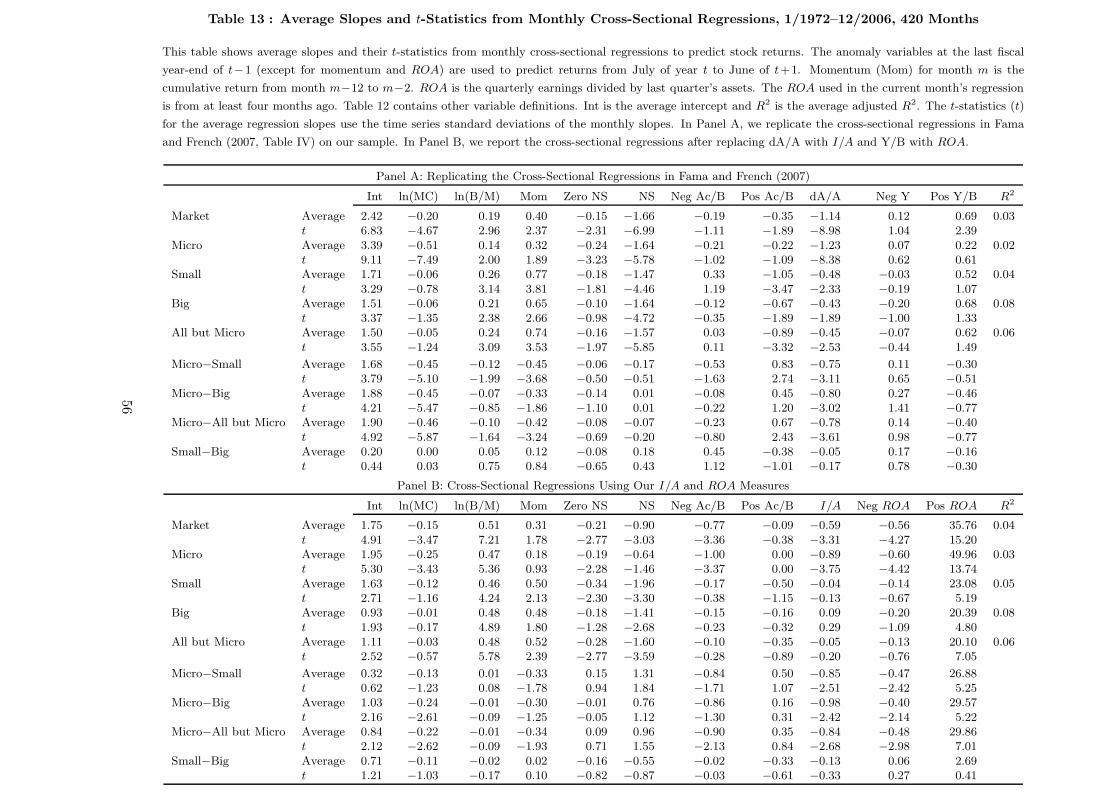
Table 13 : Average Slopes and t-Statistics from Monthly Cross-Sectional Regressions, 1/1972–12/2006, 420 Months

This table shows average slopes and their t-statistics from monthly cross-sectional regressions to predict stock returns. The anomaly variables at the last fiscal

year-end of t−1 (except for momentum and ROA) are used to predict returns from July of year t to June of t+1. Momentum (Mom) for month m is the

cumulative return from month m−12 to m−2. ROA is the quarterly earnings divided by last quarter’s assets. The ROA used in the current month’s regression

is from at least four months ago. Table 12 contains other variable definitions. Int is the average intercept and R2 is the average adjusted R2. The t-statistics (t)

for the average regression slopes use the time series standard deviations of the monthly slopes. In Panel A, we replicate the cross-sectional regressions in Fama

and French (2007, Table IV) on our sample. In Panel B, we report the cross-sectional regressions after replacing dA/A with I/A and Y/B with ROA.

Panel A: Replicating the Cross-Sectional Regressions in Fama and French (2007)

Int ln(MC) ln(B/M) Mom Zero NS NS Neg Ac/B Pos Ac/B dA/A Neg Y Pos Y/B R2

Market Average 2.42 −0.20 0.19 0.40 −0.15 −1.66 −0.19 −0.35 −1.14 0.12 0.69 0.03t 6.83 −4.67 2.96 2.37 −2.31 −6.99 −1.11 −1.89 −8.98 1.04 2.39

Micro Average 3.39 −0.51 0.14 0.32 −0.24 −1.64 −0.21 −0.22 −1.23 0.07 0.22 0.02t 9.11 −7.49 2.00 1.89 −3.23 −5.78 −1.02 −1.09 −8.38 0.62 0.61

Small Average 1.71 −0.06 0.26 0.77 −0.18 −1.47 0.33 −1.05 −0.48 −0.03 0.52 0.04t 3.29 −0.78 3.14 3.81 −1.81 −4.46 1.19 −3.47 −2.33 −0.19 1.07

Big Average 1.51 −0.06 0.21 0.65 −0.10 −1.64 −0.12 −0.67 −0.43 −0.20 0.68 0.08t 3.37 −1.35 2.38 2.66 −0.98 −4.72 −0.35 −1.89 −1.89 −1.00 1.33

All but Micro Average 1.50 −0.05 0.24 0.74 −0.16 −1.57 0.03 −0.89 −0.45 −0.07 0.62 0.06t 3.55 −1.24 3.09 3.53 −1.97 −5.85 0.11 −3.32 −2.53 −0.44 1.49

Micro−Small Average 1.68 −0.45 −0.12 −0.45 −0.06 −0.17 −0.53 0.83 −0.75 0.11 −0.30t 3.79 −5.10 −1.99 −3.68 −0.50 −0.51 −1.63 2.74 −3.11 0.65 −0.51

Micro−Big Average 1.88 −0.45 −0.07 −0.33 −0.14 0.01 −0.08 0.45 −0.80 0.27 −0.46t 4.21 −5.47 −0.85 −1.86 −1.10 0.01 −0.22 1.20 −3.02 1.41 −0.77

Micro−All but Micro Average 1.90 −0.46 −0.10 −0.42 −0.08 −0.07 −0.23 0.67 −0.78 0.14 −0.40t 4.92 −5.87 −1.64 −3.24 −0.69 −0.20 −0.80 2.43 −3.61 0.98 −0.77

Small−Big Average 0.20 0.00 0.05 0.12 −0.08 0.18 0.45 −0.38 −0.05 0.17 −0.16t 0.44 0.03 0.75 0.84 −0.65 0.43 1.12 −1.01 −0.17 0.78 −0.30

Panel B: Cross-Sectional Regressions Using Our I/A and ROA Measures

Int ln(MC) ln(B/M) Mom Zero NS NS Neg Ac/B Pos Ac/B I/A Neg ROA Pos ROA R2

Market Average 1.75 −0.15 0.51 0.31 −0.21 −0.90 −0.77 −0.09 −0.59 −0.56 35.76 0.04t 4.91 −3.47 7.21 1.78 −2.77 −3.03 −3.36 −0.38 −3.31 −4.27 15.20

Micro Average 1.95 −0.25 0.47 0.18 −0.19 −0.64 −1.00 0.00 −0.89 −0.60 49.96 0.03t 5.30 −3.43 5.36 0.93 −2.28 −1.46 −3.37 0.00 −3.75 −4.42 13.74

Small Average 1.63 −0.12 0.46 0.50 −0.34 −1.96 −0.17 −0.50 −0.04 −0.14 23.08 0.05t 2.71 −1.16 4.24 2.13 −2.30 −3.30 −0.38 −1.15 −0.13 −0.67 5.19

Big Average 0.93 −0.01 0.48 0.48 −0.18 −1.41 −0.15 −0.16 0.09 −0.20 20.39 0.08t 1.93 −0.17 4.89 1.80 −1.28 −2.68 −0.23 −0.32 0.29 −1.09 4.80

All but Micro Average 1.11 −0.03 0.48 0.52 −0.28 −1.60 −0.10 −0.35 −0.05 −0.13 20.10 0.06t 2.52 −0.57 5.78 2.39 −2.77 −3.59 −0.28 −0.89 −0.20 −0.76 7.05

Micro−Small Average 0.32 −0.13 0.01 −0.33 0.15 1.31 −0.84 0.50 −0.85 −0.47 26.88t 0.62 −1.23 0.08 −1.78 0.94 1.84 −1.71 1.07 −2.51 −2.42 5.25

Micro−Big Average 1.03 −0.24 −0.01 −0.30 −0.01 0.76 −0.86 0.16 −0.98 −0.40 29.57t 2.16 −2.61 −0.09 −1.25 −0.05 1.12 −1.30 0.31 −2.42 −2.14 5.22

Micro−All but Micro Average 0.84 −0.22 −0.01 −0.34 0.09 0.96 −0.90 0.35 −0.84 −0.48 29.86t 2.12 −2.62 −0.09 −1.93 0.71 1.55 −2.13 0.84 −2.68 −2.98 7.01

Small−Big Average 0.71 −0.11 −0.02 0.02 −0.16 −0.55 −0.02 −0.33 −0.13 0.06 2.69t 1.21 −1.03 −0.17 0.10 −0.82 −0.87 −0.03 −0.61 −0.33 0.27 0.41

56

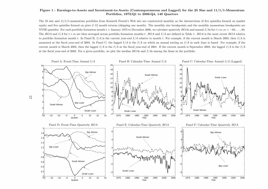
Figure 1 : Earnings-to-Assets and Investment-to-Assets (Contemporaneous and Lagged) for the 25 Size and 11/1/1-MomentumPortfolios, 1972:Q1 to 2006:Q4, 140 Quarters

The 25 size and 11/1/1-momentum portfolios from Kenneth French’s Web site are constructed monthly as the intersections of five quintiles formed on market

equity and five quintiles formed on prior 2–12 month returns (skipping one month). The monthly size breakpoints and the monthly momentum breakpoints are

NYSE quintiles. For each portfolio formation month t = January 1972 to December 2006, we calculate quarterly ROAs and annual I/As for t+m,m = −60, . . . , 60.

The ROA and I/A for t + m are then averaged across portfolio formation months t. ROA and I/A are defined in Table 1. ROA is the most recent ROA relative

to portfolio formation month t. In Panel B, I/A is the current year-end I/A relative to month t. For example, if the current month is March 2003, then I/A is

measured at the fiscal year-end of 2003. In Panel C, the lagged I/A is the I/A on which an annual sorting on I/A in each June is based. For example, if the

current month is March 2003, then the lagged I/A is the I/A at the fiscal year-end of 2001. If the current month is September 2003, the lagged I/A is the I/A

at the fiscal year-end of 2002. For a given portfolio, we plot the median ROAs and I/As among the firms in the portfolio.

Panel A: Event-Time Annual I/A Panel B: Calendar-Time Annual I/A Panel C: Calendar-Time Annual I/A (Lagged)

−20 −15 −10 −5 0 5 10 15 202

3

4

5

6

7

8

9

10

Quarter

Small−Loser

Small−WinnerBig−Loser

Big−Winner

1975 1980 1985 1990 1995 2000 2005−2

0

2

4

6

8

10

12

14

16

18

20

Year

Small−Loser

Small−Winner

1975 1980 1985 1990 1995 2000 2005−2

0

2

4

6

8

10

12

14

16

18

20

Year

Small−Loser

Small−Winner

Panel D: Event-Time Quarterly ROA Panel E: Calendar-Time Quarterly ROA Panel F: Calendar-Time Quarterly ROA

−20 −15 −10 −5 0 5 10 15 200

0.2

0.4

0.6

0.8

1

1.2

1.4

1.6

1.8

2

Quarter

Small−Loser

Small−Winner

Big−Loser

Big−Winner

1975 1980 1985 1990 1995 2000 2005

−4

−2

0

2

4

6

Year

Small−Loser

Small−Winner

1975 1980 1985 1990 1995 2000 2005

−4

−2

0

2

4

6

Year

Big−Loser

Big−Winner

57