Embed Size (px)
Citation preview
NEOGENE EXHUMATION OF THE SIKKIM HIMALAYA FROM ZIRCON (U-TH)/HE THERMOCHRONOLOGY AND 3-D THERMO-KINEMATIC MODELLING
by
Kyle R. Landry
Submitted in partial fulfillment of the requirements for the degree of Master of Science
at
Dalhousie University Halifax, Nova Scotia
August 2014
© Copyright by Kyle R. Landry, 2014
TABLE OF CONTENTS
LIST OF TABLES............................................................................................................vi
LIST OF FIGURES..........................................................................................................vii
ABSTRACT...................................................................................................................xi
LIST OF ABBREVIATIONS USED....................................................................................xii
AKNOWLEDGEMENTS................................................................................................xiv
CHAPTER 1 - INTRODUCTION........................................................................................1
1.1 - OROGEN-SCALE GEOLOGIC SETTING..............................................................2
1.2 - TECTONIC MODELS FOR NEOGENE DEVELOPMENT OF THE PRESENT OROGENIC FRONT................................................................5
CHAPTER 2 - GEOLOGICAL SETTING.............................................................................12
2.1 - INTRODUCTION.............................................................................................12
2.2 - GEOLOGY OF SIKKIM.....................................................................................12
2.2.1 - Tethyan Sedimentary Sequence (TSS) and South Tibetan Detachment Zone (STDZ)..............................................12
2.2.2 - Greater Himalayan Sequence (GHS) and Main Central Thrust Zone (MCTZ).......................................................15
2.2.3 - Lesser Himalayan Sequence (LHS) and Ramgarh Thrust (RT)..................................................................................20
2.2.4 - The Main Boundary Thrust (MBT), the Siwaliks Group and the Main Frontal Thrust (MFT).................................22
2.3 - THE RANGIT AND TISTA WINDOWS AND THE LESSER HIMALAYAN DUPLEX SYSTEM........................................................................................24
2.4 - GEOPHYSICAL DATA......................................................................................37
2.4.1 - Seismicity and GPS Data..............................................................30
2.5 - TOPOGRAPHIC DATA.....................................................................................33
CHAPTER 3 - THERMOCHRONOLOGY METHODOLOGY AND RESULTS..........................38
3.1 - INTRODUCTION.............................................................................................38
3.2 - ZIRCON (U-TH)/HE (ZHE) THERMOCHRONOLOGY: PRINCIPLES OF THE METHOD....................................................................................................38
3.2.1 - Thermochronology.....................................................................40
3.2.2 - Isotopic Decay and Effective Closure Temperature...................42
ii
3.2.3 - The Helium Partial Retention Zone............................................43
3.3 - ANALYTICAL PROCEDURE..............................................................................44
3.3.1 - Crystal Isolation..........................................................................45
3.3.2 - Grain Selection...........................................................................45
3.4 - ISOTOPE EXTRACTION AND MEASUREMENT................................................47
3.4.1 - Laser Extraction and Measurement of Helium..........................47
3.4.2 - Extraction of U and Th Isotopes.................................................49
3.4.3 - Dissolution of the Zircons...........................................................49
3.4.4 - Isotope Dilution Technique and Calculations.............................50
3.5 - AGE CALCULATION AND ALPHA-EJECTION CORRECTION.............................51
3.5.1 - U-Th/He Age Calculation............................................................51
Linear Approximation Method......................................................51
Indirect Iterative Method..............................................................52
Direct Calculation Method.............................................................53
3.5.2 - Alpha-Ejection Correction..........................................................55
3.6. OTHER ZHE CONSIDERATIONS AND ASSUMPTIONS.......................................57
3.6.1 - Presence of Pre-Existing Helium.................................................58
3.6.2 - Secular Equilibrium.....................................................................58
3.6.3 - Zonation of Parent Isotopes.......................................................59
3.6.4 - Samarium (Sm)...........................................................................59
3.7 - ZHE COOLING AGE RESULTS..........................................................................60
3.7.1 - ZHe Cooling Age Descriptions.....................................................60
CHAPTER 4 - INTERPRETATION OF ZHE AGES AND NUMERICAL MODELLING
RESULTS...............................................................................................67
4.1 - THERMAL FIELD IN THE CONTINENTAL CRUST.............................................67
4.1.1 - The Effects of Thrust Faulting on the Crustal Thermal Field................................................................................68
4.1.2 - Topographic Effects on the Thermal Structure...........................70
4.1.3 - Erosion and Sedimentation.........................................................71
iii

4.2 - THREE-DIMENSIONAL THERMOKINEMATIC MODELLING TO INTERPRET THERMOCHRONOMETER AGES..............................................73
4.2.1 - The Pecube Software.................................................................74
Kinematic Componant...................................................................75
Thermal Componant.....................................................................86
Age Prediction Componant...........................................................77
4.2.2 - Forward Modelling....................................................................78
4.3 - NEIGHBOURHOOD ALGORITHM (NA) INVERSION.........................................78
4.4 - NUMERICAL MODEL DESIGN.........................................................................80
4.5 - INVERSION RESULTS......................................................................................84
4.5.1 - Scenario 1 (Inversion SKI01).....................................................84
SKI01 Inversion Results..................................................................85
SKI01 Forward Model....................................................................86
4.5.2 - Scenario 2 (Inversion SKI02).....................................................89
SKI02 Inversion Results..................................................................90
SKI02 Forward Model....................................................................92
4.5.3 - Scenario 3 (Inversions SKI03 and SKI04)..................................94
SKI03 Inversion Results.................................................................95
SKI03 Forward Model....................................................................97
SKI04 Inversion Results.................................................................99
SKI04 Forward Model..................................................................100
CHAPTER 5 - DISCUSSION AND CONCLUSIONS...........................................................103
5.1 - TECTONIC MODELS FOR THE SIKKIM HIMALAYA........................................103
5.2 - MODELLED EXHUMATION RATES................................................................105
5.3 - COMPARISON OF MODELS ALONG STRIKE OF THE OROGEN.....................107
5.4 - LIMITATIONS OF THE MODELS....................................................................115
5.5 - TECTONIC HISTORY OF SIKKIM....................................................................117
5.6 - CONCLUSIONS.............................................................................................119
REFERENCES..............................................................................................................121
APPENDIX A..............................................................................................................141
iv

Appendix B...............................................................................................................142
v
LIST OF TABLES
Table 2.1 Stratigraphic table summarizing the lithology and thickness of the LHS units in Sikkim..........................................................20
Table 3.1 Comparison of (U-Th)/He age calculation solutions
using sample ISIK-08-03.............................................................................54 Table 3.2 Zircon (U-Th)/He cooling age results.........................................................61
Table 4.1 Model Input Parameters...........................................................................82
Table 4.2 Inversion input parameter table and results.............................................84
vi
LIST OF FIGURES
Figure 1.1 Geological map of the Himalaya showing the major geological units and bounding structures.............................................................................2
Figure 1.2 Paleomagnetic reconstruction showing the northern drift of the
Indian subcontinent from 70 Ma................................ ..............................4 Figure 1.3 Diagrams showing the three states a wedge can be in under the
critical wedge model..................................................................................7 Figure 1.4 Tectonic models of the Himalayan wedge for the late Neogene...............9
Figure 2.1 Geological map of Sikkim..........................................................................13 Figure 2.2 Interpretative section across the Sikkim Himalaya showing the main
geological units and structures..................................................................14 Figure 2.3 Schematic cross-section showing the sequence of metamorphic
isograds increasing from lower (LHS) to higher (GHS) structural levels along an E-W profile in central Sikkim.............................................17
Figure 2.4 Schematic diagram showing the Rangit duplex.........................................25 Figure 2.5 Interpretative reconstruction of the formation of the Rangit Duplex.......26 Figure 2.6 Location of receiver function profiles from Acton et al., 2011 and
seismic profiles from INDEPTH..................................................................28 Figure 2.7 Results of a receiver function survey through the Sikkim
Himalaya along the profile A-A’ shown in Figure 2.6, combined with INDEPTH data for the northern part of the transect.........................29
Figure 2.8 Composite results of INDEPTH reflection profiles extending
from 27°43’ to the 30°35’..........................................................................30 Figure 2.9 North-south section across Sikkim (at ~88.6 °E) showing the
depths of the epicenters of major modern earthquakes..........................31 Figure 2.10 Map of northern India, the eastern Himalaya and Tibet
showing GPS velocity vectors....................................................................32 Figure 2.11 Topographic map of Nepal, Sikkim and Bhutan showing
the location of four 20 km wide topographic profiles..............................33
vii
Figure 2.12 Four topographic profiles from the foreland to the high Himalaya in Nepal (A) Annapurna and B) Langtang) and (C) Western and (D) Eastern Bhutan........................................................34
Figure 2.13 Digital Elevation Model of Sikkim between 26.5 °N - 28 °N
and 88 °E - 89 °E.......................................................................................36 Figure 2.14 A swath profile constructed along the zone indicted in
Figure 2.10...............................................................................................37 Figure 3.1 Geologic map of Sikkim showing the geographical and
geological location of the samples...........................................................39
Figure 3.2 Particle trajectory during thrust-faulting.................................................41 Figure 3.3 Temperature range of the HePRZ for the apatite, zircon and
titanite (U-Th)/He systems.......................................................................44 Figure 3.4 Grain ISIK-08-38-1 measurements...........................................................46 Figure 3.5 Ejection, retention, or implantation of α-particles within a
euhedral zircon........................................................................................56 Figure 3.6 a) Cross section through Sikkim showing sample cooling
ages in relation to the major geological units and structures.................65 Figure 3.7 Distribution of cooling ages with respect to elevation............................66 Figure 4.1 Effects of topography and thrust faulting on the thermal
structure of the upper crust.....................................................................69 Figure 4.2 Modelled effects of surface topography in three-dimensions
on the apatite helium (60°C) and apatite fission track (110° C) closure isotherms at Mt. Waddington, BC, Canada................................71
Figure 4.3 Effects of erosion rate on cooling ages of different
thermochronometers..............................................................................72 Figure 4.4 Depth-temperature plots showing how the geothermal
gradient changes over time during sedimentation and erosion at a constant rate of 1 mm/yr....................................................73
viii
Figure 4.5 General set-up of thermokinematic models with relevant thermal and kinematic parameters and an example of the resulting thermal and velocity fields.............................83
Figure 4.6 Inversion results for model SKI01 solving for six free
parameters.............................................................................................87 Figure 4.7 Observed cooling ages (blue) and associated 1 Ma
error plotted with the predicted cooling ages (red) from the lowest misfit forward model from inversion SKI01.......................................................................................................88
Figure 4.8 Thermal field, velocity field and MHT geometry
produced by inversion SKI01..................................................................88 Figure 4.9 Inversion results for model SKI02 solving for eight
free parameters......................................................................................92 Figure 4.10 Observed cooling ages (blue) and associated 1 Ma
error plotted with the predicted cooling ages (red) from the forward model with the lowest misfit from inversion SKI02........................................................................................93
Figure 4.11 Thermal and velocity field for forward model SKI02..............................94 Figure 4.12 Inversion results for model SKI03 solving for four
free parameters......................................................................................96 Figure 4.13 Observed cooling ages (blue) and associated 1 Ma
error plotted against the predicted cooling ages (red) from the lowest misfit forward model from inversion SKI03.......................................................................................................97
Figure 4.14 The thermal and velocity field for SKI03 shown in two
time-steps to show the effects of the duplex zone over a period less than the 12 Ma model run................................................98
Figure 4.15 Inversion results for model SKI04 solving for four free
parameters...........................................................................................100 Figure 4.16 Observed cooling ages (blue) and associated 1 Ma error
plotted with the predicted cooling ages (red) from the forward model with the lowest misfit in inversion SKI04....................100
ix
Figure 4.17 The thermal and velocity field for forward model SKI04 shown in two time-steps to illustrate the effects of the duplex zone over a period of time less than the 12 Ma model run.............................................................................................102
Figure 5.1 a) Exhumation rates, b)cooling ages and topography, c) best fit model design........................................................................106
Figure 5.2 Compilation of low temperature thermochronology data and tectonic models across the central and eastern Himalaya.................112
Figure 5.3 A simplified schematic model showing the proposed
tectonic evolution of Sikkim in three stages........................................118
x
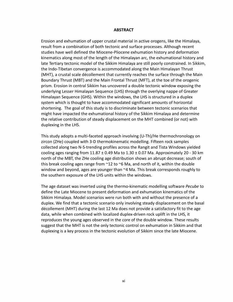
ABSTRACT
Erosion and exhumation of upper crustal material in active orogens, like the Himalaya, result from a combination of both tectonic and surface processes. Although recent studies have well defined the Miocene-Pliocene exhumation history and deformation kinematics along most of the length of the Himalayan arc, the exhumational history and late Tertiary tectonic model of the Sikkim Himalaya are still poorly constrained. In Sikkim, the Indo-Tibetan convergence is accommodated along the Main Himalayan Thrust (MHT), a crustal scale décollement that currently reaches the surface through the Main Boundary Thrust (MBT) and the Main Frontal Thrust (MFT), at the toe of the orogenic prism. Erosion in central Sikkim has uncovered a double tectonic window exposing the underlying Lesser Himalayan Sequence (LHS) through the overlying nappe of Greater Himalayan Sequence (GHS). Within the windows, the LHS is structured in a duplex system which is thought to have accommodated significant amounts of horizontal shortening. The goal of this study is to discriminate between tectonic scenarios that might have impacted the exhumational history of the Sikkim Himalaya and determine the relative contribution of steady displacement on the MHT combined (or not) with duplexing in the LHS. This study adopts a multi-faceted approach involving (U-Th)/He thermochronology on zircon (ZHe) coupled with 3-D thermokinematic modelling. Fifteen rock samples collected along two N-S-trending profiles across the Rangit and Tista Windows yielded cooling ages ranging from 11.87 ± 0.49 Ma to 1.30 ± 0.07 Ma. Approximately 20 - 30 km north of the MBT, the ZHe cooling age distribution shows an abrupt decrease; south of this break cooling ages range from ~12 to ~6 Ma, and north of it, within the double window and beyond, ages are younger than ~4 Ma. This break corresponds roughly to the southern exposure of the LHS units within the windows. The age dataset was inverted using the thermo-kinematic modelling software Pecube to define the Late Miocene to present deformation and exhumation kinematics of the Sikkim Himalaya. Model scenarios were run both with and without the presence of a duplex. We find that a tectonic scenario only involving steady displacement on the basal décollement (MHT) during the last 12 Ma does not provide a satisfactory fit to the age data, while when combined with localized duplex-driven rock uplift in the LHS, it reproduces the young ages observed in the core of the double window. These results suggest that the MHT is not the only tectonic control on exhumation in Sikkim and that duplexing is a key process in the tectonic evolution of Sikkim since the late Miocene.
xi
LIST OF ABBREVIATIONS USED
TSS Tethyan Sedimentary Sequence
STDZ South Tibetan Detachment Zone
GHS Greater Himalayan Sequence
MCTZ Main Central Thrust Zone
HHT High Himalayan Thrust
MCT Main Central Thrust
LHS Lesser Himalayan Sequence
RT Ramgarh Thrust
MBT Main Boundary Thrust
MFT Main Frontal Thrust
MHT Main Himalayan Thrust
GPS Global Positioning System
ZHe Zircon (U-Th)/He
NA Neighbourhood Algorithm
Ma Mega Anum (Million Years)
AFT Apatite Fission Track
OSL Optically Stimulated Luminescence
TSL Thermally Stimulated Luminescence
LVZ Low Velocity Zone
INDEPTH International Deep Profiling of Tibet and the Himalaya
ITRF International Terrestrial Reference Frame
xii
SRTM Shuttle Radar Topography Mission
DEM Digital Elevation Model
HePRZ Helium Partial Retention Zone
SPT Sodium Polytungstate
MI Diiodomethane
UCSC University of California Santa Cruz
ICP-MS Inductively Coupled Mass Spectrometer
HF Hydrofluoric Acid
HNO3 Nitric Acid
SA/V Surface Area to Volume Ratio
Ga Giga Anum (Billion Years)
ka Kilo Anum (Thousand Years)
PDF Probability Density Function
xiii

ACKNOWLEDGEMENTS
I’d first and foremost like to thank my supervisor, Isabelle Coutand, whose patience and
guidance have been instrumental in encouraging me to both start and complete this
thesis. Also, Dave Whipp was invaluable in helping me to both use Pecube and
understand how it works. I’d like to thank my committee members (Dave Whipp, Martin
Gibling and John Gosse) for their constructive comments on various parts of the project
and especially on the final submission. Keith Taylor and Jeremy Hourrigan (UCSC) were
instrumental in helping me complete my age analysis. I’d like to thank all of the rest of
the faculty and staff in the Earth Sciences department at DAL for all the help and support
given to me over the past two degrees. Finally I’d like to thank the other grad students
who have worked and studied with me over the past three years for the good times had.
xiv
Chapter 1 - Introduction
The mechanisms which control exhumation across the Himalayan orogen and the
interactions between them have seen substantial debate over the past decade. Erosion
and exhumation of the Himalaya are controlled by the interactions between tectonic
and climatic processes (e.g., Beaumont et al., 2001; Hodges et al., 2004; Grujic et al.,
2006; Whipple and Meade, 2006; Whipple, 2009). In convergent orogens, tectonic
processes such as thrust faults transport material towards the surface while climatic
processes and associated surface processes (e.g. river erosion, mass movement) erode
the surface. The net result is exhumation (or burial where sedimentation outpaces
erosion). However, the contribution of tectonic processes to the observed upper crustal
exhumation and the mechanisms by which they have done so remain poorly
constrained. This study adopts a multi-faceted approach, coupling (U-Th)/He
thermochronology on zircons and 3D-thermokinematic Modelling, to test and refine
conceptual tectonic models for the Eastern Himalaya in Sikkim (India) and to highlight
the key tectonic mechanisms that may have contributed to the late Neogene (12 Ma to
present) development of this part of the orogen. Previous thermochronological and
modelling studies have primarily focused on the western and central Himalaya where
findings about crustal deformation, exhumation, and the resulting thermal structure
have been extrapolated to other parts of the orogen (e.g., Gansser, 1964; Avouac, 2003;
Bollinger et al., 2004; Hodges 2004; Wobus et al., 2005; Herman et al., 2010; Robert et
al., 2011). However, the applicability of previous studies to the Sikkim Himalaya is
limited because this part of the range is located in a transition zone between Nepal to
1
the west (e.g., Whipp et al., 2007, Herman et al., 2010) and Bhutan to the east (e.g.,
Grujic et al., 2006; Coutand et al., 2014) (Figure 1.1), each area having different
structural and morphological characteristics. These along-strike variations are detailed in
Chapter 2.
1.1 - Orogen-Scale Geologic Setting
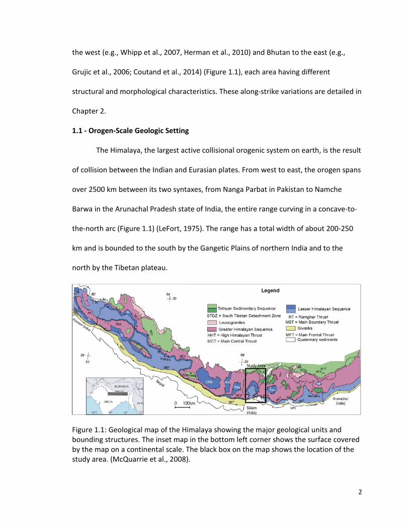
The Himalaya, the largest active collisional orogenic system on earth, is the result
of collision between the Indian and Eurasian plates. From west to east, the orogen spans
over 2500 km between its two syntaxes, from Nanga Parbat in Pakistan to Namche
Barwa in the Arunachal Pradesh state of India, the entire range curving in a concave-to-
the-north arc (Figure 1.1) (LeFort, 1975). The range has a total width of about 200-250
km and is bounded to the south by the Gangetic Plains of northern India and to the
north by the Tibetan plateau.
Figure 1.1: Geological map of the Himalaya showing the major geological units and bounding structures. The inset map in the bottom left corner shows the surface covered by the map on a continental scale. The black box on the map shows the location of the study area. (McQuarrie et al., 2008).
2
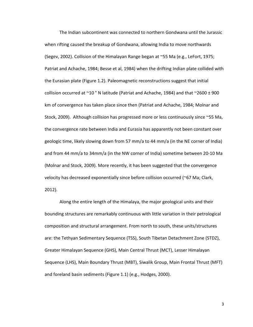
The Indian subcontinent was connected to northern Gondwana until the Jurassic
when rifting caused the breakup of Gondwana, allowing India to move northwards
(Segev, 2002). Collision of the Himalayan Range began at ~55 Ma (e.g., LeFort, 1975;
Patriat and Achache, 1984; Besse et al, 1984) when the drifting Indian plate collided with
the Eurasian plate (Figure 1.2). Paleomagnetic reconstructions suggest that initial
collision occurred at ~10 ° N latitude (Patriat and Achache, 1984) and that ~2600 ± 900
km of convergence has taken place since then (Patriat and Achache, 1984; Molnar and
Stock, 2009). Although collision has progressed more or less continuously since ~55 Ma,
the convergence rate between India and Eurasia has apparently not been constant over
geologic time, likely slowing down from 57 mm/a to 44 mm/a (in the NE corner of India)
and from 44 mm/a to 34mm/a (in the NW corner of India) sometime between 20-10 Ma
(Molnar and Stock, 2009). More recently, it has been suggested that the convergence
velocity has decreased exponentially since before collision occurred (~67 Ma; Clark,
2012).
Along the entire length of the Himalaya, the major geological units and their
bounding structures are remarkably continuous with little variation in their petrological
composition and structural arrangement. From north to south, these units/structures
are: the Tethyan Sedimentary Sequence (TSS), South Tibetan Detachment Zone (STDZ),
Greater Himalayan Sequence (GHS), Main Central Thrust (MCT), Lesser Himalayan
Sequence (LHS), Main Boundary Thrust (MBT), Siwalik Group, Main Frontal Thrust (MFT)
and foreland basin sediments (Figure 1.1) (e.g., Hodges, 2000).
3
Figure 1.2: Paleomagnetic reconstruction showing the northern drift of the Indian subcontinent from 70 Ma, through collision at ~55 Ma and to the present. Each anomaly represents a specific magnetic reversal which was dated and correlated with the location of the Indian subcontinent at that time. The red dashed lines show the relative motion of two static points on the subcontinent. The grey shaded section shows the current position of India. (From Patriat and Achache, 1984).
The TSS is a Cambrian to Eocene low-grade metasedimentary sequence
(Gansser, 1964; Gaetani and Garzanti, 1991) bounded to the north in Tibet by the Indus-
Tsangpo Suture, the boundary between the Indian and Eurasian plates, and to the south
by the northward-dipping normal-sense shear zone known as the STDZ. Structurally
4
below and to the south of the STDZ is the GHS, a series of medium-to-high
metamorphic-grade gneisses, metasediments, and migmatites intruded by Miocene
leucogranites (e.g., Hodges, 2000). It is bounded to the south by the MCT ductile shear
zone, which overlies an 8-10 km thick package of Proterozoic to Permian marine
metasedimentary rocks known as the LHS (e.g., Hodges, 2000). The base of the LHS is
bounded to the south by the MBT, the second oldest major north-dipping thrust fault in
the Himalayan range front, which is a fairly narrow zone (<100 m wide) of cataclasis
(Schelling, 1992; Meigs et al 1995). To the south of the MBT are strata of the Siwalik
Group, a series of syn-orogenic sedimentary rocks derived from the eroded material of
topographically and structurally higher units and deposited in the foreland basin (e.g.,
Gansser, 1983). The southern boundary of the Siwaliks is the MFT, the youngest of the
major south-propagating thrust faults and active toe of the orogen. The MFT, MBT and
MCT branch at depth from the Main Himalayan Thrust (MHT; Nelson et al., 1996) which
is the basal detachment of the modern Himalayan orogenic wedge.
1.2 - Tectonic Models for Neogene Development of the Present Orogenic Front
Different models have been used to explain different parts of the growth history
of the Himalaya. One of these is the channel flow model (e.g., Beaumont et al., 2001;
2004; Grujic et al., 2002; Godin et al., 2006) which involves the lateral migration,
extrusion and exhumation of partially molten mid-crustal material due to localized
climatically-induced surface erosion. Exhumation occurs through concurrent and
opposite displacement on structures bounding the paleo-channel. In the Himalayan case
the GHS is bounded by two north-dipping opposite-sense shear zones, the thrust-sense
5

MCT in the south and normal-sense STDZ in the north, both active from at least the Early
Miocene (~23 Ma) until the late Middle Miocene (~10 Ma at the latest; e.g., Godin et al.,
2006; Grujic et al., 2006; Harris et al., 2006; Catlos et al., 2007). Channel flow is a ductile
process; it can only occur at temperatures above the brittle-ductile transition. Thus
when the channel rocks cooled, exhumation of material continued through brittle
processes (Grujic et al., 2006) such as thrusting along newer major north-dipping faults
(e.g., MBT), or re-activation of older shear zones (e.g., MCT). Metamorphic petrology
coupled with geochronology suggests that in the eastern Bhutan Himalaya channel flow,
and associated ductile deformation, ceased by ~10 Ma (e.g., Grujic et al., 2011).
Deformation in the cooler upper crust occurs for the most part in brittle fashion
and can be described using the critical wedge model (Davis et al., 1983), commonly
applied to active fold-and-thrust belts (e.g., Dahlen, 1990). The wedge features (Dahlen,
1990; Figure 1.3) a basal décollement (a large orogen-scale thrust fault) with a dip angle
of β along which the wedge slides. The average topographic surface of the wedge has an
angle, α. The angle α+β is called the taper of the wedge and can be used to determine
what state the wedge is in. The taper can be modified through changes in erosion,
sedimentation or internal deformation.
6
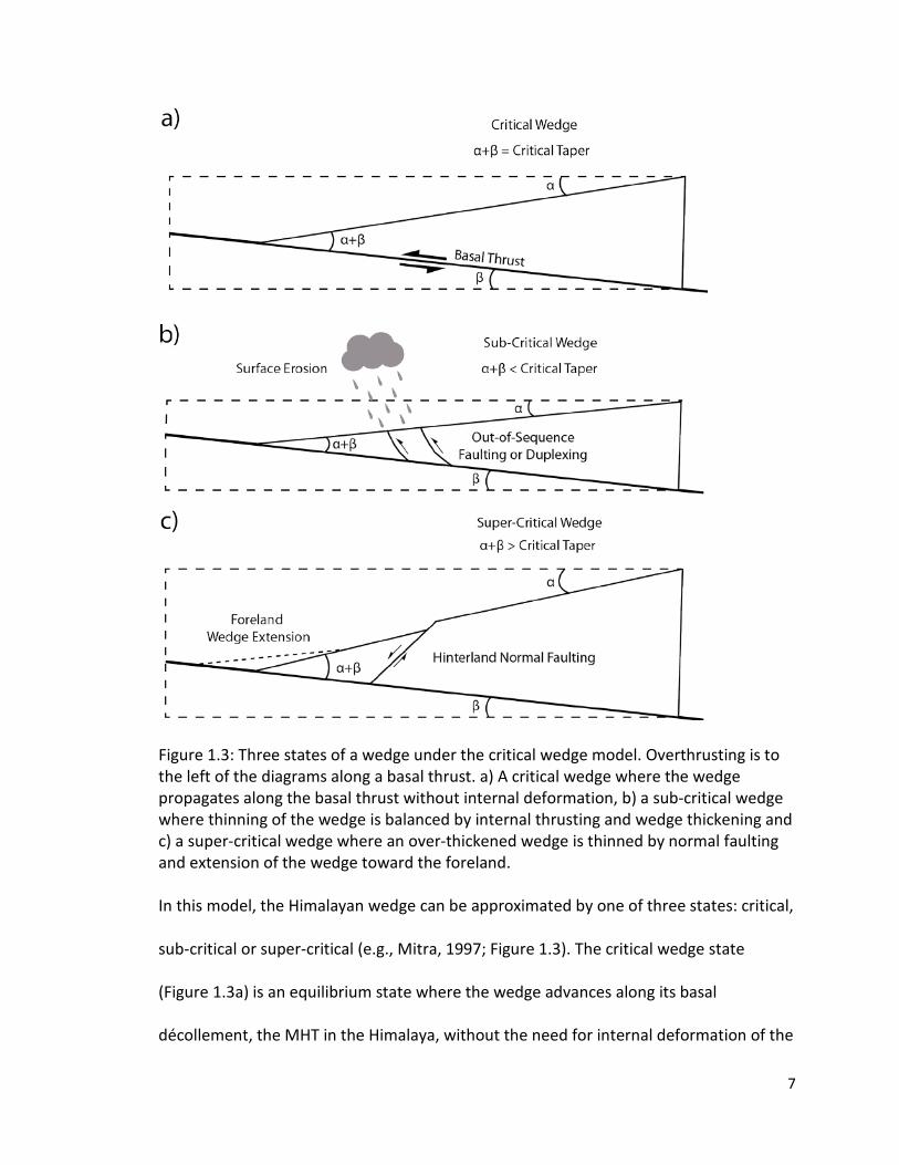
Figure 1.3: Three states of a wedge under the critical wedge model. Overthrusting is to the left of the diagrams along a basal thrust. a) A critical wedge where the wedge propagates along the basal thrust without internal deformation, b) a sub-critical wedge where thinning of the wedge is balanced by internal thrusting and wedge thickening and c) a super-critical wedge where an over-thickened wedge is thinned by normal faulting and extension of the wedge toward the foreland. In this model, the Himalayan wedge can be approximated by one of three states: critical,
sub-critical or super-critical (e.g., Mitra, 1997; Figure 1.3). The critical wedge state
(Figure 1.3a) is an equilibrium state where the wedge advances along its basal
décollement, the MHT in the Himalaya, without the need for internal deformation of the
7

wedge, which grows via basal accretion. This occurs when a critical taper angle (α+β) is
maintained through a balance of forces that thicken and thin the wedge. A sub-critical
state (Figure 1.3b) occurs when the taper of the wedge is at an angle shallower than the
critical taper, due to erosion at the surface, and the wedge must thicken internally
through the formation of out-of-sequence thrusts and duplexes. A super-critical state
(Figure 1.3c) occurs in the case where the taper is at an angle higher than the critical
taper and must compensate through normal faulting in order to extend the wedge and
lower the angle of repose. In the cases of both sub- and super-critical wedges, the
purpose of internal deformation is to return to the equilibrium state of the critical
wedge (Davis et al., 1983). It has been suggested from activity on presumed out-of-
sequence faults north of the MFT that the Sikkim wedge may be in a sub-critical state
(Mukul, 2000). While the Sikkim range-front can be approximated to first order to have
been a critical wedge since at least 10 Ma, the tectonic model that best describes the
evolution of the wedge during that time frame is still under debate.
It is important to note that the channel flow and critical wedge models are not
mutually exclusive. While these two models describe different processes, Jamieson and
Beaumont (2013) showed that the models can coexist within the Himalaya with brittle
critical wedge mechanics governing the fold-thrust belt to the south of the exhumed
channel and that they can occur contemporaneously.
There are currently three major tectonic models to account for the development
of the frontal part of the Himalaya from the Late Miocene to the present (Figures 1.4 a-
c):
8

Figure 1.4: Tectonic models of the Himalayan wedge for the late Neogene. a) Model of a wedge overthrusting the foreland on a geometrically variable basal décollement (MHT). Grey arrows show the particle pathway on both sides of the décollement. b) Out-of-sequence thrusting in a wedge in sub-critical state. c) Development of a duplex at mid-to-upper crustal depths above a crustal ramp. Black arrows show the area where underplating is occurring (Modified after Herman et al., 2010).
The first model involves overthrusting of the orogenic wedge on a major crustal-
scale basal décollement with a ramp-and-flat geometry (e.g., Gansser, 1964, Herman et
al., 2010; Robert et al., 2009, 2011) (Figure 1.4a). The basal décollement, the MHT, is
characterized by ramp-and-flat sections as constrained by geophysical data (e.g., Nelson
et al., 1996; Alsdorf et al., 1998; Nábělek et al, 2009; Acton et al., 2011). In this model,
enhanced exhumation occurs at the surface above the ramp segments due to the more
vertical particle path combined with steady-state topography (Robert et al., 2011;
Coutand et al., 2014). Robert et al., (2009; 2011) used thermokinematic Modelling of
thermochronologic data to suggest that lateral changes in the MHT geometry may be
the primary control of upper crustal exhumation along the orogen.
The second model involves the growth of a mid-crustal duplex on top of a ramp
segment of the MHT (e.g., Avouac, 2003, Bollinger et al., 2004, Herman et al., 2010)
9
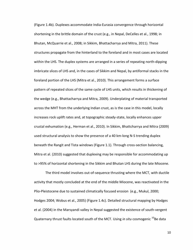
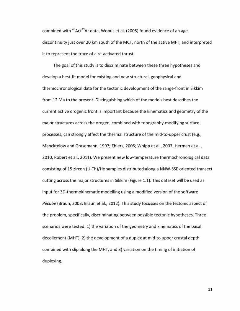
(Figure 1.4b). Duplexes accommodate India-Eurasia convergence through horizontal
shortening in the brittle domain of the crust (e.g., in Nepal, DeCelles et al., 1998; in
Bhutan, McQuarrie et al., 2008; in Sikkim, Bhattacharrya and Mitra, 2011). These
structures propagate from the hinterland to the foreland and in most cases are located
within the LHS. The duplex systems are arranged in a series of repeating north-dipping
imbricate slices of LHS and, in the cases of Sikkim and Nepal, by antiformal stacks in the
foreland portion of the LHS (Mitra et al., 2010). This arrangement forms a surface
pattern of repeated slices of the same cycle of LHS units, which results in thickening of
the wedge (e.g., Bhattacharrya and Mitra, 2009). Underplating of material transported
across the MHT from the underlying Indian crust, as is the case in this model, locally
increases rock uplift rates and, at topographic steady-state, locally enhances upper
crustal exhumation (e.g., Herman et al., 2010). In Sikkim, Bhattcharrya and Mitra (2009)
used structural analysis to show the presence of a 40 km-long N-S trending duplex
beneath the Rangit and Tista windows (Figure 1.1). Through cross-section balancing,
Mitra et al. (2010) suggested that duplexing may be responsible for accommodating up
to >95% of horizontal shortening in the Sikkim and Bhutan LHS during the late Miocene.
The third model involves out-of-sequence thrusting where the MCT, with ductile
activity that mostly concluded at the end of the middle Miocene, was reactivated in the
Plio-Pleistocene due to sustained climatically focused erosion (e.g., Mukul, 2000;
Hodges 2004; Wobus et al., 2005) (Figure 1.4c). Detailed structural mapping by Hodges
et al. (2004) in the Marsyandi valley in Nepal suggested the existence of south-vergent
Quaternary thrust faults located south of the MCT. Using in situ cosmogenic 10Be data
10
combined with 40Ar/39Ar data, Wobus et al. (2005) found evidence of an age
discontinuity just over 20 km south of the MCT, north of the active MFT, and interpreted
it to represent the trace of a re-activated thrust.
The goal of this study is to discriminate between these three hypotheses and
develop a best-fit model for existing and new structural, geophysical and
thermochronological data for the tectonic development of the range-front in Sikkim
from 12 Ma to the present. Distinguishing which of the models best describes the
current active orogenic front is important because the kinematics and geometry of the
major structures across the orogen, combined with topography-modifying surface
processes, can strongly affect the thermal structure of the mid-to-upper crust (e.g.,
Mancktelow and Grasemann, 1997; Ehlers, 2005; Whipp et al., 2007, Herman et al.,
2010, Robert et al., 2011). We present new low-temperature thermochronological data
consisting of 15 zircon (U-Th)/He samples distributed along a NNW-SSE oriented transect
cutting across the major structures in Sikkim (Figure 1.1). This dataset will be used as
input for 3D-thermokinematic modelling using a modified version of the software
Pecube (Braun, 2003; Braun et al., 2012). This study focusses on the tectonic aspect of
the problem, specifically, discriminating between possible tectonic hypotheses. Three
scenarios were tested: 1) the variation of the geometry and kinematics of the basal
décollement (MHT), 2) the development of a duplex at mid-to upper crustal depth
combined with slip along the MHT, and 3) variation on the timing of initiation of
duplexing.
11
Chapter 2 - Geological Setting
2.1 – Introduction
The Indian Province of Sikkim is located in the eastern Himalayan orogen
between Nepal to the west, Bhutan to the east, and Tibet to the north (Figure 1.1).
Although the major geological units and structures in Sikkim are, on first approximation,
similar to those observed at the scale of the orogen (see Chapter 1), the Sikkim Himalaya
presents unique lithological, structural and geomorphological features that I introduce in
detail in this chapter.
2.2 – Geology of Sikkim
2.2.1 - Tethyan Sedimentary Sequence (TSS) and South Tibetan Detachment Zone (STDZ) The Tethyan Sedimentary Sequence (TSS) has been mapped as a continuous unit
in the northern part of Sikkim and extends northwards into Tibet (Figure 2.1). However,
it has not been formally described in Sikkim and observations from neighbouring Nepal
and Bhutan (e.g., Garzanti 1999; Kellett et al., 2012) are used here. It is composed of
unmetamorphosed to greenschist facies marine shales and carbonates, associated with
continental sandstones and conglomerates of Devonian to Jurassic age (Gaetani and
Garzanti, 1999; Kellett et al., 2012). The sequence overlies a discontinuous higher-grade
unit of greenschist-to-amphibolite-grade metasediments (Gansser, 1964) locally known
as the Chekha Group in Bhutan or the Everest Group in Nepal (e.g., Kellett et al., 2012).
An isolated slice of slate and schist overlain by sandstone, quartzite and marble mapped
within the TSS in northwestern Sikkim (Pan et al., 2004) has similar metamorphic
12
characteristics and occupies the same structural level as the Chekha Group in Bhutan
(Kellett et al., 2013), and may be an equivalent unit.
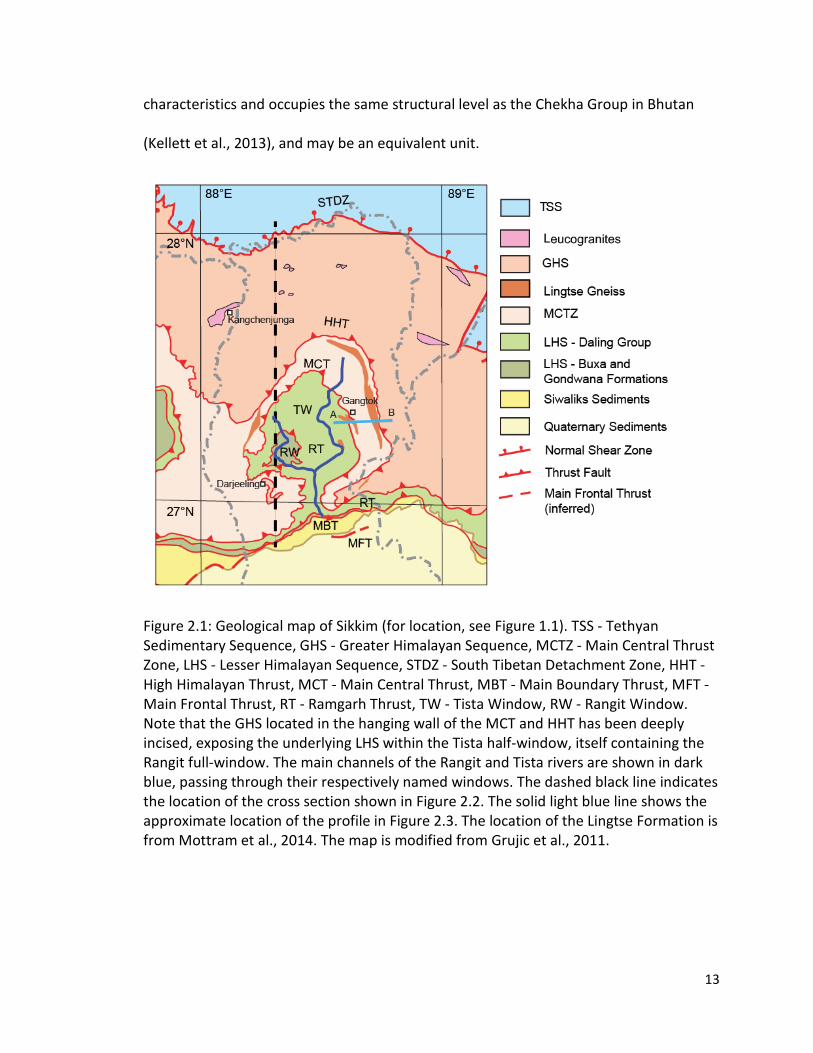
Figure 2.1: Geological map of Sikkim (for location, see Figure 1.1). TSS - Tethyan Sedimentary Sequence, GHS - Greater Himalayan Sequence, MCTZ - Main Central Thrust Zone, LHS - Lesser Himalayan Sequence, STDZ - South Tibetan Detachment Zone, HHT - High Himalayan Thrust, MCT - Main Central Thrust, MBT - Main Boundary Thrust, MFT - Main Frontal Thrust, RT - Ramgarh Thrust, TW - Tista Window, RW - Rangit Window. Note that the GHS located in the hanging wall of the MCT and HHT has been deeply incised, exposing the underlying LHS within the Tista half-window, itself containing the Rangit full-window. The main channels of the Rangit and Tista rivers are shown in dark blue, passing through their respectively named windows. The dashed black line indicates the location of the cross section shown in Figure 2.2. The solid light blue line shows the approximate location of the profile in Figure 2.3. The location of the Lingtse Formation is from Mottram et al., 2014. The map is modified from Grujic et al., 2011.
13
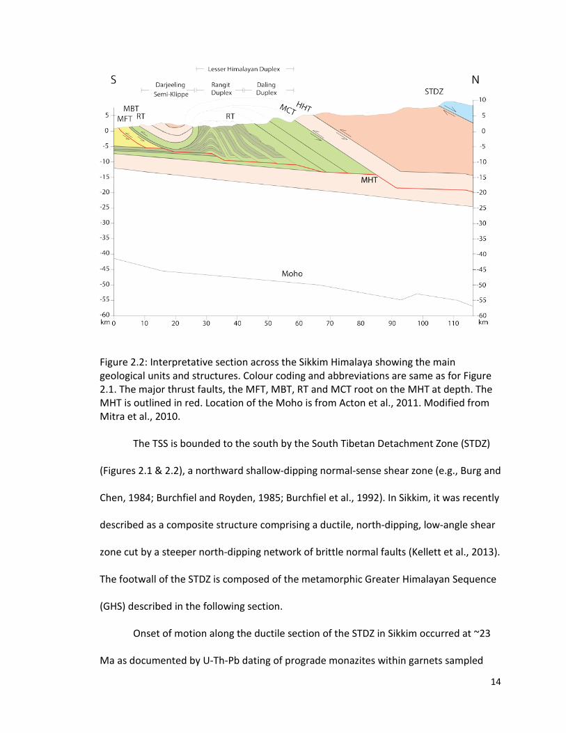
Figure 2.2: Interpretative section across the Sikkim Himalaya showing the main geological units and structures. Colour coding and abbreviations are same as for Figure 2.1. The major thrust faults, the MFT, MBT, RT and MCT root on the MHT at depth. The MHT is outlined in red. Location of the Moho is from Acton et al., 2011. Modified from Mitra et al., 2010.
The TSS is bounded to the south by the South Tibetan Detachment Zone (STDZ)
(Figures 2.1 & 2.2), a northward shallow-dipping normal-sense shear zone (e.g., Burg and
Chen, 1984; Burchfiel and Royden, 1985; Burchfiel et al., 1992). In Sikkim, it was recently
described as a composite structure comprising a ductile, north-dipping, low-angle shear
zone cut by a steeper north-dipping network of brittle normal faults (Kellett et al., 2013).
The footwall of the STDZ is composed of the metamorphic Greater Himalayan Sequence
(GHS) described in the following section.
Onset of motion along the ductile section of the STDZ in Sikkim occurred at ~23
Ma as documented by U-Th-Pb dating of prograde monazites within garnets sampled
14

from the STDZ footwall (Kellett et al., 2013). U-Pb dating of undeformed leucogranites
(i.e., no ductile shearing) located in the footwall (< 5 km south of the STDZ) suggests
that ductile motion ended by ~13 Ma, about 2 Ma earlier than in neighbouring Bhutan
(Kellett et al., 2009). AFT (apatite fission track) and AHe (Apatite (U-Th)/He) data from
one leucogranite sample located in the immediate footwall of the STDZ yielded near-
identical ages of 12.9 ± 0.7 and 12.8 ± 0.8 Ma, respectively, indicating very fast cooling
from temperatures of about 400°C, and are interpreted as representing the timing of
ductile activity on the STDZ in Sikkim. 40Ar/39Ar data on muscovites from these
leucogranites yielded total gas ages ranging from 12.4 ± 0.7 to 13.3 ± 0.4 Ma, within the
same range to slightly older than the AFT and AHe ages from the same samples. Finally,
biotite and muscovite 39Ar/40Ar ages in the Sa’er region between Sikkim and Nepal show
rapid cooling after the end of ductile deformation between 13.6 and 11 Ma suggesting
that brittle activity ceased at that point (Leloup et al., 2010).
2.2.2 - Greater Himalayan Sequence (GHS) and Main Central Thrust Zone (MCTZ)
The Greater Himalayan Sequence (GHS) is exposed in the footwall of the STDZ
(Figure 2.1) and is composed of high-grade metamorphic rocks of both igneous and
sedimentary origin intruded by leucogranites, as observed elsewhere in the Himalaya
(e.g., LeFort, 1975; Schwan, 1980; Hodges, 2000). The high-grade metamorphic
crystalline rocks of Sikkim are divided into the Darjeeling and Lingste Formations (e.g.,
Acharya, 1975). The predominant Darjeeling Formation (also known as the Darjeeling
Gneiss Unit) is composed of stromatic migmatites of pelitic origin, associated with less
common calc-silicates, metabasites, augen gneisses and minor quartzites (Ghosh, 1968;
15

Neogi et al., 1998). The GHS is exposed in the hanging wall of the MCTZ and extends
northwards to the STDZ; it is also found further south where remnants are preserved in
the Darjeeling klippe (Figure 2.1) (e.g., Mohan et al., 1989). The Lingtse Formation (or
Lingtse Gneiss) is present in isolated slivers located structurally above both the MCTZ
and LHS to the south (e.g., Mohan et al 1989; Mottram et al., 2014; Figure 2.1). The unit
is composed of pelitic schists, psammites, quartzites, calc-silicates and orthogneiss (Paul
et al., 1982; Neogi et al., 1998), is well foliated to highly mylonitized (Dasgupta et al.,
2009), and has been used in previous studies as a marker for the location of the MCT
shear zone (e.g., Neogi et al., 1998).
In Sikkim the MCT shear zone is represented by a 10 - 15 km wide zone of GHS
rocks that have undergone ductile deformation, referred to as the MCTZ (Figures 2.1 &
2.2, e.g., Neogi et al., 1998; Harris et al., 2004; Mottram et al., 2014). It is bounded by
two north-dipping thrust-sense shear zones variably called MCT1 and MCT (e.g., Catlos
et al., 2004), MCT2 and MCT1 (e.g., Bhattcharyya and Mitra, 2009) or MCT and HHT
(High Himalayan Thrust; e.g., Grujic et al., 2011) for the southern and northern
structures, respectively (Figures 2.1 & 2.2). The terminology MCT and HHT will be used
herein. The rocks present in the MCTZ are known as the Paro Formation (e.g., Acharya
1975) and are primarily composed of biotite-muscovite schists (Harris et al., 2004). The
MCTZ, along with the upper LHS and lower GHS, preserves an inverted metamorphic
sequence documented across the Himalaya (e.g., Mohan et al., 1989, MacFarlane et al.,
1995; Harrison et al., 1997; Grujic et al., 2002) where the metamorphic grade
progressively increases towards higher structural levels (from the LHS to the GHS).
16

Across the MCTZ the metamorphic grade increases from chlorite + biotite grade in the
Daling schists of the LHS, increasing to the garnet-, staurolite-, kyanite- and sillimanite-in
isograds, and finally to the sillimanite+K-feldspar-in isograd over a horizontal distance of
10-15 km, ending in the southernmost GHS. The schists show a progressive increase in
pressure-temperature conditions from 480°C and peak pressure of 4.8 kbars at the top
of the LHS to 715°C and 8.4 kbars in the GHS in the north (Figure 2.3; Mohan et al., 1989;
Harris et al., 2004; Dasgupta et al., 2004, 2009; Mottram et al., 2014).
Figure 2.3: Schematic cross-section showing the sequence of metamorphic isograds increasing from lower (LHS) to higher (GHS) structural levels along an E-W profile in central Sikkim (for location, see Figure 2.1). Abbreviations are: Chl - Chlorite, Bt - Biotite, Grt - Garnet, St - Staurolite, Ky - Kyanite, Sil - Sillimanite, Mus - Muscovite. A mineral followed by -in signifies that it is the first time the mineral was encountered (the lowest pressure/temperature) along the section; -out signifies that the mineral no longer occurs at temperatures/pressures beyond that point. Modified from Dasgupta et al., 2004, sillimanite isograds from Mottram et al., 2014.
Based on pressure-temperature data and compositional zoning of garnets found
within migmatites in the footwall of the STDZ, the northern section of the GHS may have
experienced peak metamorphic conditions of up to ~10 kbars and 800 °C (Ganguly et al.,
17
2000). Retrograde mineral reactions within garnet and cordierite combined with
thermobarometric Modelling suggest initial rapid exhumation of the GHS at a rate of ~15
mm/yr from a depth of ~34 km to 14.7 km followed by a brief period of heating and
rapid cooling to 11.8 km and finally a much slower phase of exhumation at ~2 mm/yr to
a depth of ~5 km below the surface. If this rate is extrapolated for the last 5 km of
exhumation to the surface, then the GHS would have been exhumed to the surface from
a depth of ~34 km over a period of ~8 Ma, corresponding to an average exhumation rate
of 4.25 mm/yr (Ganguly et al., 2000).
Leucogranites intruding the GHS and the TSS are found as dykes, sills and plutons
up to several kilometres size directly related to the anatexis of the GHS; partial melting
due to muscovite dehydration caused differentiation of the GHS resulting in felsic
intrusions into the rest of the GHS and overlying TSS (LeFort et al., 1987; Harris and
Massey, 1994; Zhang et al., 2004). The ages of these leucogranites has been constrained
by U-Th-Pb chronology and trace element analyses on zircons and monazites and
suggests that emplacement occurred primarily between 23-22 Ma and 13-12 Ma (e.g.,
Parrish et al., 1992; Rubatto et al., 2012; Kellett et al., 2013). In Sikkim, the majority of
these leucogranites are found in the NW corner of the province, in and around the
Kangchenjunga massif (Figure 2.1, Searle and Szulc, 2005).
Several studies used both geo-and thermochronological dating methods to
constrain the chronology of tectonic movement on the MCTZ in Sikkim. Catlos et al.
(2004) used Th-Pb dating on monazite from GHS samples from the hanging wall of the
MCT, and LHS samples from the footwall on the northeastern edge of the Tista Window
18
(Figure 2.1). The oldest monazites are located in the footwall of the HHT and range in
age from 22.0 ± 0.3 to 20.1 ± 0.7 Ma; these results are interpreted as representing the
crystallization ages of the monazites formed during the first movement along the MCTZ
(Catlos et al., 2004). A younger group of ages ranging from 18.3±0.1 to 12.9±0.2 Ma
derived from samples from the footwalls of both the HHT and the MCT are interpreted
to represent monazite growth during shearing across the MCTZ and date the onset of
ductile deformation along the MCT. Finally, the youngest group of samples from the
MCT footwall range from 11.9±0.3 to 10.3±0.2 Ma which suggests that the MCT was
active until at least 10 Ma (Catlos et al., 2004).
Garnets from migmatites and granites located in the hanging wall of the MCTZ
(Harris et al., 2004) yielded Sm-Nd ages of 16.1 ± 2.4 Ma and 23 ± 2.6 Ma, from rim and
core respectively, and are interpreted as representing different periods of garnet
growth. Incidentally, the age of the core of the garnet coincides with the onset of
activity on the MCT (~20-23 Ma) as determined by Catlos et al. (2004); Harris et al (2004)
further suggested that the age of the cores may represent the onset of significant
displacement on the MCT, whereas the age of the rims may represent younger
movement episodes. From these and other geochronological studies in other parts of
the orogen (c.f., Figure 4 in Godin et al., 2006) it is suggested that the MCTZ was active
between ~23 Ma and ~10 Ma.
The GHS and the MCTZ were thrust over the LHS along the MCT (Figure 2.2). The
convoluted modern trace of the MCT in map view results from differential erosion
affecting the GHS nappe which exposes the underlying LHS in the Tista half-window
19

(Figure 2.1). Away from this peculiar erosional feature both HHT and MCT are parallel to
the E-W trend of the major Himalayan structures (Figure 2.1).
2.2.3 - Lesser Himalayan Sequence (LHS) and Ramgarh Thrust (RT)
The LHS exposed in Sikkim consists of three units: the Daling Group, the Buxa
Formation and the Gondwana Formation (e.g., Schwan, 1980; Bhattacharrya and Mitra,
2009; Figures 2.1 & 2.2, Table 2.1).
Table 2.1: Summary of the lithologies and stratigraphic thicknesses of the LHS units (Daling, Buxa and Gondwana) in Sikkim. From Mitra et al., 2010.
The oldest but structurally highest LHS unit, the Precambrian Daling group,
consists of the quartzitic Reyang Formation and the overlying meta-pelitic Daling
Formation (Bhattacharrya and Mitra, 2009). The Daling Group has a maximum
stratigraphic thickness of approximately 5 km (Bhattacharrya and Mitra, 2009) and is
primarily composed of green-grey chloritic slates and phyllites of marine origin
(Bhattacharrya and Mitra, 2009; 2011). There are no data available on the age of the
20
section in Sikkim; however equivalent formations have been dated in both Bhutan and
Nepal. U-Pb dates on detrital zircon from the Ranimata and Kushma formations in Nepal,
which can be correlated with the Daling and Reyang formations, respectively, suggest a
maximum depositional age of ~1.86 to ~1.83 Ga (DeCelles et al., 2001). Dates from the
Daling and Shumar Formations, which can be correlated with the Reyang Formation in
Bhutan, suggest a maximum depositional age of ~1.8 - 1.9 Ga (McQuarrie et al., 2008;
Long et al., 2011).
The Buxa Formation unconformably overlies the Daling Group and is composed
of both marine and continental carbonaceous slates and interbedded quartzites,
limestones and conglomerates up to 1.2 km thick (Bhattacharrya and Mitra, 2009). The
Buxa Formation is interpreted to be Late Precambrian on the basis of marine
microfossils found within cherts in the Rangit window (Schopf et al., 2008). U-Pb dates
on detrital zircons from the equivalent Baxa Formation in Bhutan, however, suggest a
maximum Early Cambrian (520 - 485 Ma) depositional age (McQuarrie et al., 2008; Long
et al., 2011).
At the top of the sequence but at the lowest structural level, the Gondwana
Formation lies unconformably on the Buxa Formation. It is an up to 1 km thick section of
basal conglomerates overlain by sandstones, quartzites, and topped by carbonaceous
slates (Bhattacharrya and Mitra, 2009). Plant fossils found within the Gondwana
formation suggest a Permian depositional age, with deposition in a subaerial
environment (Acharyya, 1971).
21
The Ramgarh Thrust (RT) is a prominent thrust fault located within the LHS,
separating the Daling Group from the Buxa and Gondwana formations (Figures 2.1 and
2.2; Bhattacharrya and Mitra, 2009). It is exposed (1) within the double window at the
boundary between the Rangit and Tista windows and (2) to the south along strike of the
orogen between the MCT and the MBT (Figure 2.1). The RT is suggested to have been
active in western Nepal by ~15 Ma (Pearson and DeCelles, 2005) based on the minimum
age of the Dumri Formation, a synorogenic sedimentary unit stratigraphically located
above the Gondwana Formation in Nepal, exposed in the footwall of the RT. No absolute
or relative timing of activity is available for the RT in Sikkim. During the formation of the
Rangit Duplex, the rocks were folded and eroded resulting in the circular pattern now
observed at the surface and the shape of the Rangit window (Figure 2.1; Bhattacharrya
and Mitra, 2009).
2.2.4 - The Main Boundary Thrust (MBT), the Siwalik Group and the Main Frontal Thrust (MFT)
The LHS is bounded to the south by the MBT, a thrust fault dipping steeply (~50°)
towards the NNE (Mukul, 2000) (Figures 2.1 and 2.2). In Bhutan, the MBT is suggested to
have been active after about 10 Ma, when displacement associated with ductile
deformation on the MCT ceased (Coutand et al., 2014). Similar reasoning applies in
Sikkim where the MCTZ became inactive by 12-10 Ma. It is likely that the MBT became
active at that time in order to accommodate ongoing convergence (Catlos et al., 2004;
Harris et al., 2004).
The Siwalik Group is a sequence of syn-orogenic clastic sediments derived from
the erosion of material from structurally higher units (e.g., GHS, LHS), transported and
22
deposited into the Himalayan foreland basin. The Siwaliks can be subdivided into three
lithotectonic units termed the lower, middle and upper Siwaliks, all of alluvial origin
(Burbank et al., 1996). The lower unit is predominantly mudstones, the middle unit
sandstones, and the upper unit is defined by a large proportion of conglomerates
(Najman, 2006). No information is available for the thickness of the Siwaliks in Sikkim,
but elsewhere in the Himalaya it ranges from less than 3 km in eastern Bhutan, to over
7.5 km in northwestern India (e.g., Hirschmiller et al., 2013).
The southern boundary of the Siwaliks is the Main Frontal Thrust (MFT), the
southernmost thrust fault in the orogenic wedge and the currently active frontal toe of
the Himalaya (Lavé and Avouac, 2000; Lavé and Avouac, 2001). The MFT is only
discontinuously exposed at the surface (e.g., Figure 2.1) and thrusts the Siwalik Group
on top of the modern foreland basin. Mukul et al. (2007) combined optically and
thermally stimulated luminescence ages (OSL and TSL) from fault gouge from the MFT
and obtained an age of ~40 ka which was interpreted as reflecting ongoing activity on
the MFT into the late Pleistocene. In Nepal, Lavé and Avouac (2000) examined offset
fluvial terraces and concluded that during the Holocene, the MFT accommodated an
average of 21.5 mm/yr of N-S shortening during periodic slip events. Similar geomorphic
work on offset fluvial terraces was conducted in Bhutan and yielded an average rate of
~20 mm/yr during the last 2 ka (Berthet et al., 2014).
The MFT, MBT and MCT all branch at depth from the Main Himalayan Thrust
(MHT) (Figure 2.2) (e.g., Schelling and Arita, 1991; Nelson et al., 1996), a crustal-scale
décollement along which the Himalayan wedge is being thrust on top of the Himalayan
23

foreland basin and the Indian craton to the south (Figure 2.2). The MHT has been
imaged through geophysical surveys (e.g., Zhao et al., 1993; Nelson et al., 1996; Acton et
al 2011) and its location and geometry are detailed in section 2.4.
2.3 - The Rangit and Tista Windows and the Lesser Himalayan Duplex System
Among the most striking geological features observed in Sikkim are the two
erosional windows which expose the LHS units beneath the GHS (Bhattacharyya and
Mitra, 2009; Figures 2.1 and 2.2). The larger Tista half-window is bounded by an
irregular circular MCT map pattern (Figure 2.1) within which is exposed the smaller full
Rangit window which is delimited by the folded RT (Figure 2.2). The Rangit and the Tista
rivers, which flow through the center of their respectively named windows (Figure 2.1),
have likely played a significant role in incising and exposing the LHS units (Bhattacharyya
and Mitra, 2009).
Structural and stratigraphic analysis suggests that the LHS units are structurally
repeated, forming a system of imbricated duplexes which have been eroded resulting in
the windows on the surface (Bhattacharrya and Mitra, 2009; Mitra et al., 2010) (Figures
2.1 & 2.2). Figure 2.4 outlines the major components of a duplex.
The Daling duplex, bounded to the north by the MCT (Figure 2.2) is interpreted to
contain up to four horses of the Daling group rocks. The roof thrust (the upper bounding
thrust) of the Daling duplex system is the RT, which is soled by the MHT (Figure 2.2). The
horses dip towards the north at an angle of ~ 30° (Bhattacharrya and Mitra, 2009; Figure
2.2). In the Rangit duplex further south, four horses are stacked in a similar orientation
to those observed in the north, but involve the repetition of all three LHS units (Daling,
24
Buxa and Gondwana) (Figures 2.2 & 2.5). In the central part of the Rangit Duplex, several
LHS slices have been stacked, creating a double antiformal stack. Gravity (Bouguer
anomaly) Modelling suggests a total thickness of up to 12 km of stacked LHS units in
central Sikkim, thinning both to the east and west (Tiwari et al., 2006). Finally, south of
the antiformal stacks, there are several small imbricates that have been translated over
the top/roof of the stacks and now dip to the south (Figure 2.5).
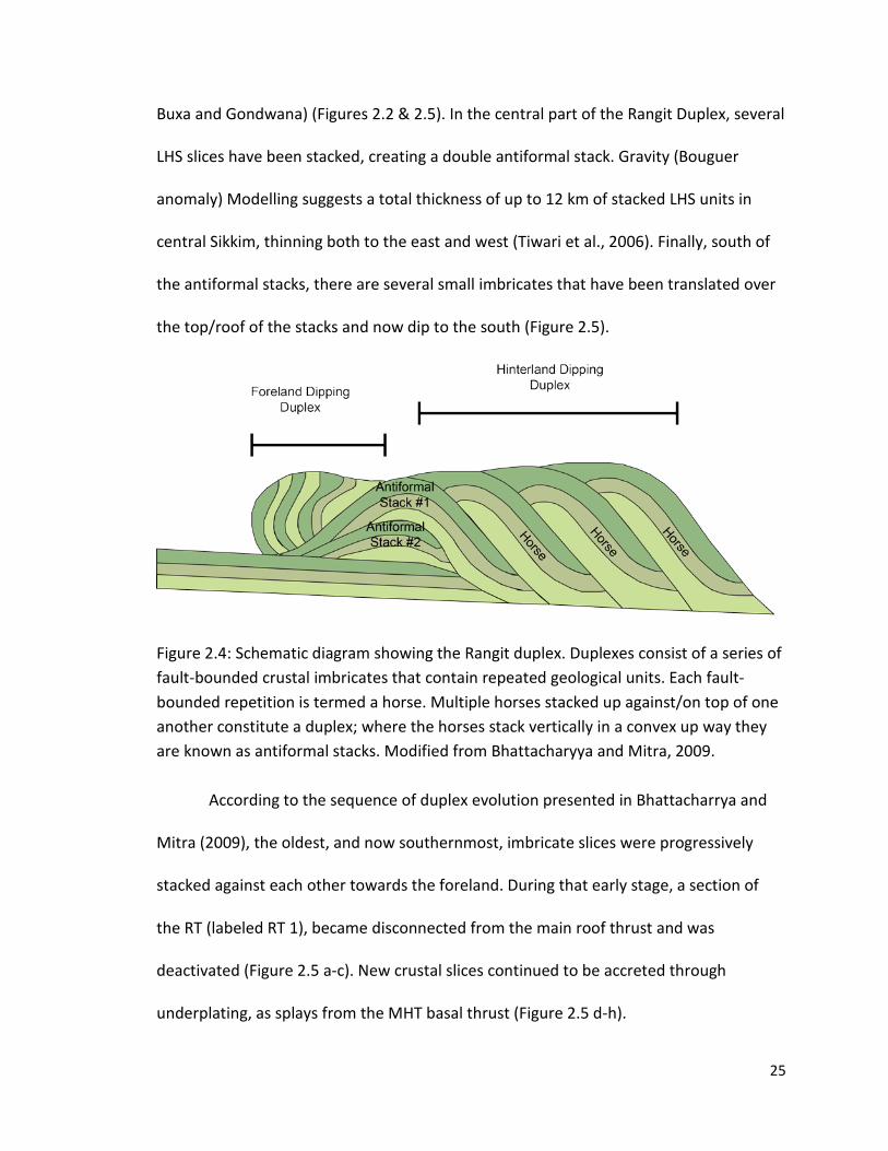
Figure 2.4: Schematic diagram showing the Rangit duplex. Duplexes consist of a series of fault-bounded crustal imbricates that contain repeated geological units. Each fault-bounded repetition is termed a horse. Multiple horses stacked up against/on top of one another constitute a duplex; where the horses stack vertically in a convex up way they are known as antiformal stacks. Modified from Bhattacharyya and Mitra, 2009.
According to the sequence of duplex evolution presented in Bhattacharrya and
Mitra (2009), the oldest, and now southernmost, imbricate slices were progressively
stacked against each other towards the foreland. During that early stage, a section of
the RT (labeled RT 1), became disconnected from the main roof thrust and was
deactivated (Figure 2.5 a-c). New crustal slices continued to be accreted through
underplating, as splays from the MHT basal thrust (Figure 2.5 d-h).
25
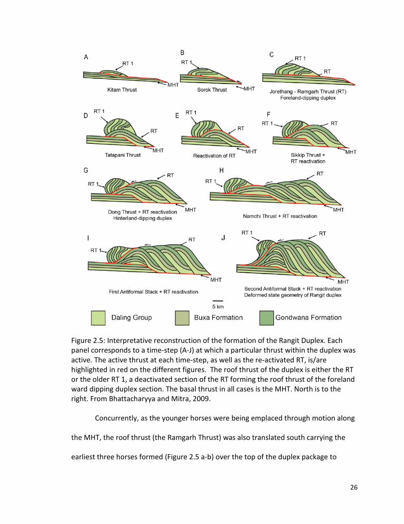
Figure 2.5: Interpretative reconstruction of the formation of the Rangit Duplex. Each panel corresponds to a time-step (A-J) at which a particular thrust within the duplex was active. The active thrust at each time-step, as well as the re-activated RT, is/are highlighted in red on the different figures. The roof thrust of the duplex is either the RT or the older RT 1, a deactivated section of the RT forming the roof thrust of the foreland ward dipping duplex section. The basal thrust in all cases is the MHT. North is to the right. From Bhattacharyya and Mitra, 2009.
Concurrently, as the younger horses were being emplaced through motion along
the MHT, the roof thrust (the Ramgarh Thrust) was also translated south carrying the
earliest three horses formed (Figure 2.5 a-b) over the top of the duplex package to
26
become the current foreland dipping horses (Figure 2.5 e-j). Finally, horses began to
stack vertically beneath growing antiformal stacks and rotating the foreland-dipping
duplex to its current position (Figure 2.5 i-j). According to this interpreted
reconstruction, the antiformal stacks are located above a ramp in the MHT (Figures 2.2
& 2.5). At a crustal ramp, the trajectory of material advected by a fault has a larger
vertical component, which equates to a local increase in rock uplift rates above the
ramp.
South of the Rangit duplex, remnants of GHS preserved in the Darjeeling klippe
(Figure 2.1) suggest that the GHS nappe once extended further south than its current
surface trace, and was eroded, exposing the underlying LHS (Figures 1.1 and 2.1)
(Bhattacharrya and Mitra, 2009).
2.4 – Geophysical Data
Several geophysical studies have found evidence of a discontinuity at depth that
corresponds to the location of the MHT. Using deep reflection seismic data, Project
International Deep Profiling of Tibet and the Himalaya (INDEPTH) (Alsdorf et al., 1998a;
Alsdorf et al., 1998b; Hauck et al., 1998; Makovsky et al., 1996; Nelson et al., 1996; Zhao
et al., 1993) imaged a strong reflector beneath the Tethyan Himalaya that is interpreted
to be the MHT underneath northern Sikkim and southern Tibet (e.g., Zhao et al., 1993;
Nelson et al., 1996 Hauck et al., 1998; Figure 2.6). The reflection data show a discrete
structure, first imaged just south of the STDZ at ~28 km depth (Figures 2.7 & 2.8) and
dipping gently (average dip ~9°) to the north in northern Sikkim and into Tibet. The
structure dips sharply below the southern limb of the Kangmar dome (~28°45’N)
27
beneath the Tethyan Himalaya, to a depth of ~50 km under southern Tibet where it
disappears from the profile (Nelson et al., 1996; Figure 2.8).
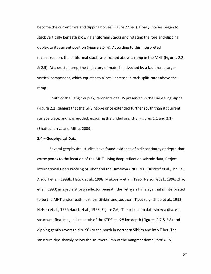
Figure 2.6: Location of receiver function profiles A-A’ and B-B’ from Acton et al., 2011 (shown in black) as well as the locations of profiles Tib-1 and Tib-2 from the INDEPTH survey (shown in red; e.g., Hauck et al., 1998) and profile T2 (in blue) showing the location of the earthquake hypocenter cross-section shown in Figure 2.9 (De and Kayal, 2003). Modified after Acton et al., 2011.
In Sikkim, Acton et al. (2011) used receiver function data, combined with
INDEPTH reflection data (Hauck et al., 1998) to image the structures at depth and
reported a distinct Low Velocity Zone (LVZ) beneath the Darjeeling-Sikkim Himalaya
(Figures 2.6 & 2.7) which they interpreted to be the MHT. The trace of the LVZ was
imaged at a depth of 10 - 15 km as a nearly flat feature beneath the lesser Himalaya
from 90 - 150 km along the A-A’ profile (SW-NE across Sikkim; Figures 2.6 & 2.7), 10 - 70
km north of the MBT. The LVZ then begins to dip (~20 - 30 °) northwards before
disappearing entirely at ~260 km along their profile, corresponding to a distance of ~160
28
km north of the MBT, at a depth of ~ 35 km (Figure 2.7). The connection between the
MHT imaged by Acton et al. (2011) and the frontal structures of the wedge (MBT and
MFT) remains unconstrained (Figure 2.7). Their second profile B-B’ (Figure 2.6), imaged
structures at similar locations and depths.
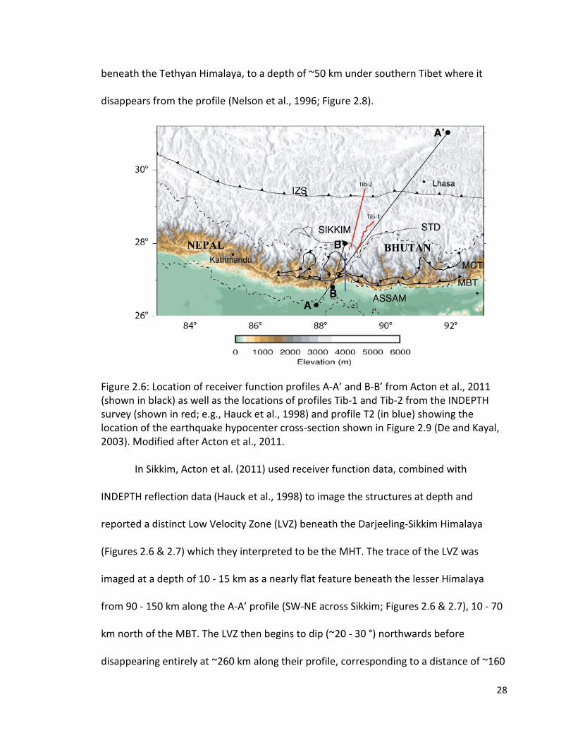
Figure 2.7: Results of a receiver function survey through the Sikkim Himalaya along the profile A-A’ shown in Figure 2.6, combined with INDEPTH data for the northern part of the transect. A Low Velocity Zone (blue) starting at ~10 km depth has been interpreted to represent the trace of the basal MHT. A high velocity zone (red) is also seen at ~50 km depth and likely represents the Moho. Discrete velocity zones (either high or low) generally represent either a geologic contact or other abrupt change in rock properties. The flat MHT begins to dip northwards beneath the HHT and continues to do so until the signal is lost. Interpretations of seismic reflection data from the INDEPTH survey (Hauck et al., 1998) show both the MHT and the Moho underneath southern Tibet and provide a reliable continuation of Acton et al’s interpretations. From Acton et al., 2011.
Both INDEPTH and Acton et al. (2011) data also imaged the Moho along the same
profiles. Acton et al. (2011) reported the depth of the Moho to be 44 - 48 km under the
29
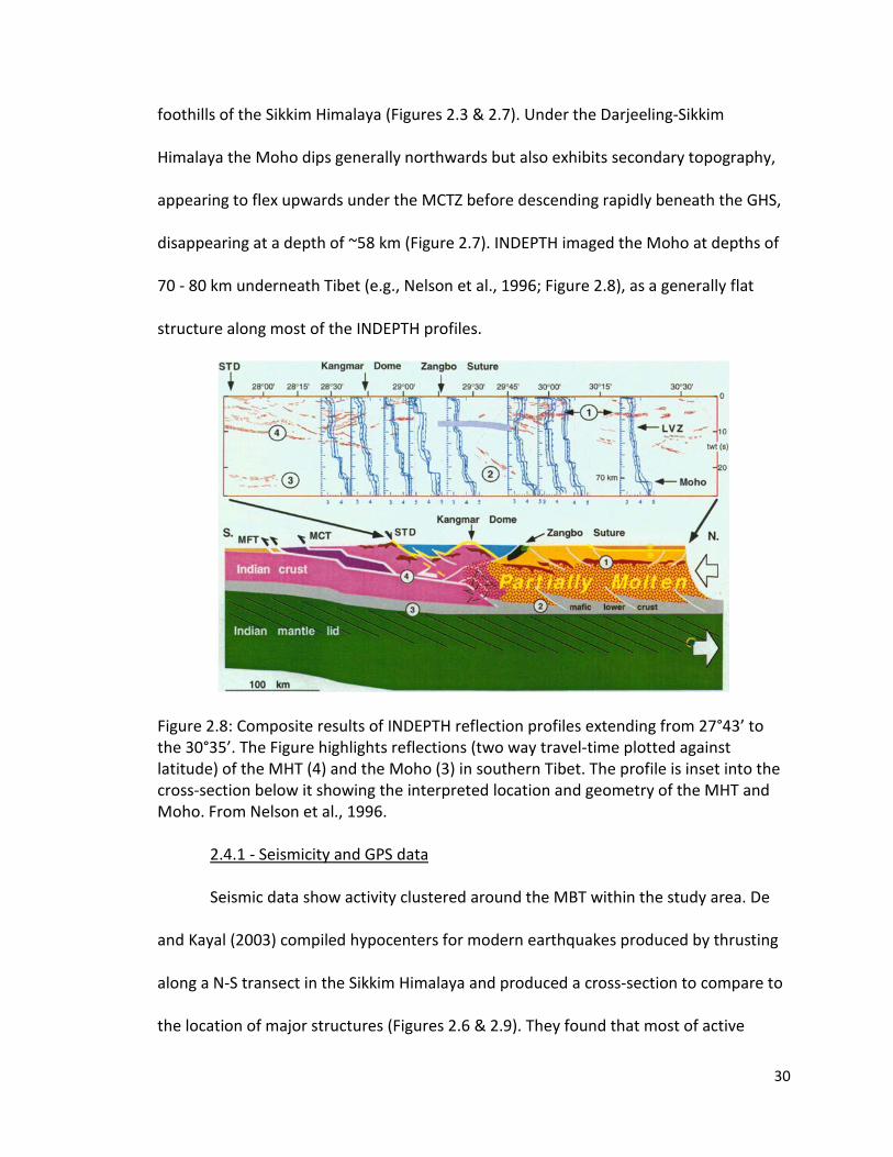
foothills of the Sikkim Himalaya (Figures 2.3 & 2.7). Under the Darjeeling-Sikkim
Himalaya the Moho dips generally northwards but also exhibits secondary topography,
appearing to flex upwards under the MCTZ before descending rapidly beneath the GHS,
disappearing at a depth of ~58 km (Figure 2.7). INDEPTH imaged the Moho at depths of
70 - 80 km underneath Tibet (e.g., Nelson et al., 1996; Figure 2.8), as a generally flat
structure along most of the INDEPTH profiles.
Figure 2.8: Composite results of INDEPTH reflection profiles extending from 27°43’ to the 30°35’. The Figure highlights reflections (two way travel-time plotted against latitude) of the MHT (4) and the Moho (3) in southern Tibet. The profile is inset into the cross-section below it showing the interpreted location and geometry of the MHT and Moho. From Nelson et al., 1996.
2.4.1 - Seismicity and GPS data
Seismic data show activity clustered around the MBT within the study area. De
and Kayal (2003) compiled hypocenters for modern earthquakes produced by thrusting
along a N-S transect in the Sikkim Himalaya and produced a cross-section to compare to
the location of major structures (Figures 2.6 & 2.9). They found that most of active
30
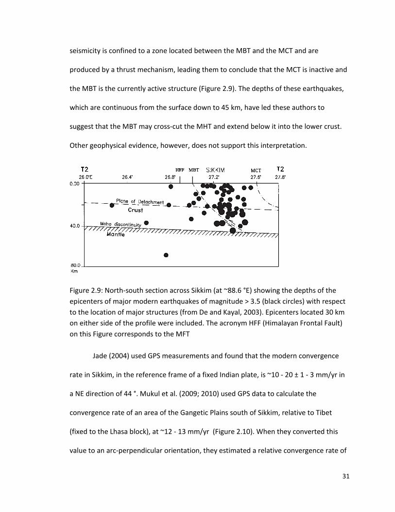
seismicity is confined to a zone located between the MBT and the MCT and are
produced by a thrust mechanism, leading them to conclude that the MCT is inactive and
the MBT is the currently active structure (Figure 2.9). The depths of these earthquakes,
which are continuous from the surface down to 45 km, have led these authors to
suggest that the MBT may cross-cut the MHT and extend below it into the lower crust.
Other geophysical evidence, however, does not support this interpretation.
Figure 2.9: North-south section across Sikkim (at ~88.6 °E) showing the depths of the epicenters of major modern earthquakes of magnitude > 3.5 (black circles) with respect to the location of major structures (from De and Kayal, 2003). Epicenters located 30 km on either side of the profile were included. The acronym HFF (Himalayan Frontal Fault) on this Figure corresponds to the MFT
Jade (2004) used GPS measurements and found that the modern convergence
rate in Sikkim, in the reference frame of a fixed Indian plate, is ~10 - 20 ± 1 - 3 mm/yr in
a NE direction of 44 °. Mukul et al. (2009; 2010) used GPS data to calculate the
convergence rate of an area of the Gangetic Plains south of Sikkim, relative to Tibet
(fixed to the Lhasa block), at ~12 - 13 mm/yr (Figure 2.10). When they converted this
value to an arc-perpendicular orientation, they estimated a relative convergence rate of
31
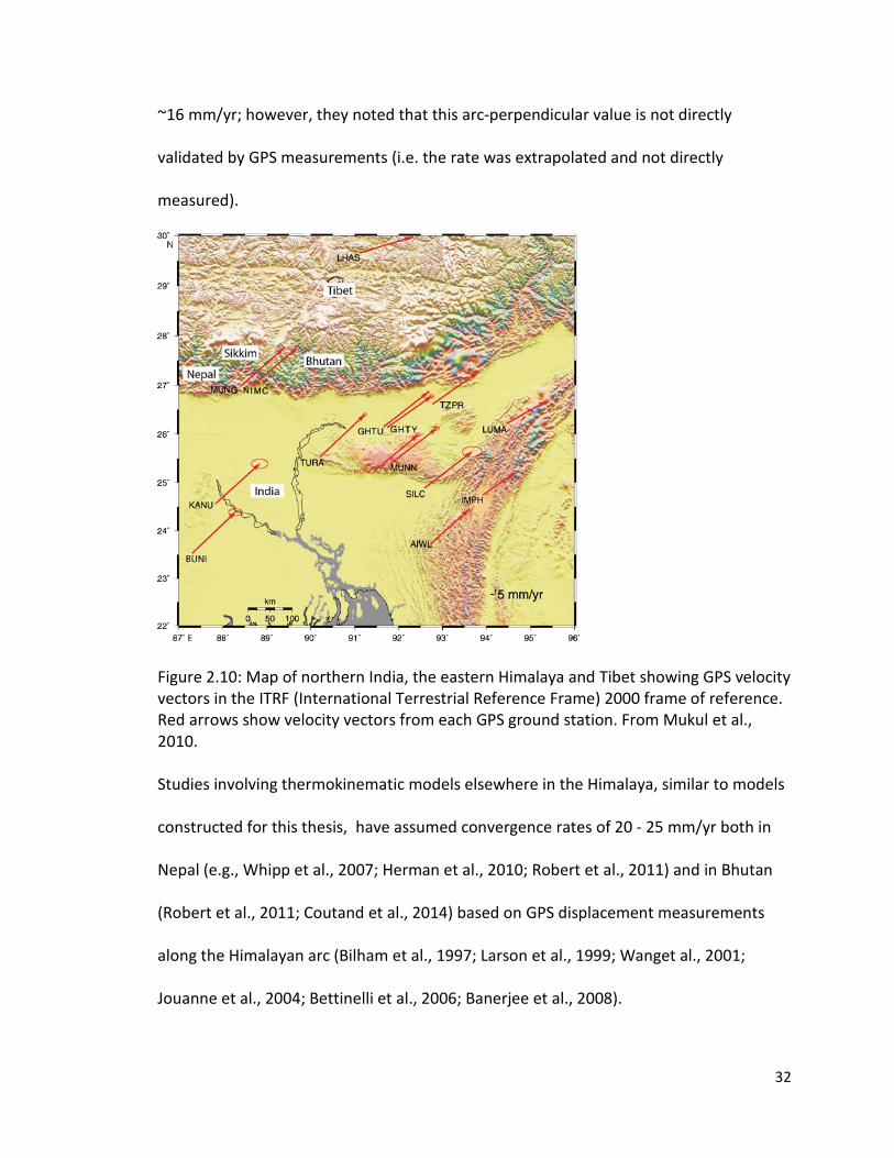
~16 mm/yr; however, they noted that this arc-perpendicular value is not directly
validated by GPS measurements (i.e. the rate was extrapolated and not directly
measured).
Figure 2.10: Map of northern India, the eastern Himalaya and Tibet showing GPS velocity vectors in the ITRF (International Terrestrial Reference Frame) 2000 frame of reference. Red arrows show velocity vectors from each GPS ground station. From Mukul et al., 2010. Studies involving thermokinematic models elsewhere in the Himalaya, similar to models
constructed for this thesis, have assumed convergence rates of 20 - 25 mm/yr both in
Nepal (e.g., Whipp et al., 2007; Herman et al., 2010; Robert et al., 2011) and in Bhutan
(Robert et al., 2011; Coutand et al., 2014) based on GPS displacement measurements
along the Himalayan arc (Bilham et al., 1997; Larson et al., 1999; Wanget al., 2001;
Jouanne et al., 2004; Bettinelli et al., 2006; Banerjee et al., 2008).
32
2.5 – Topographic Data
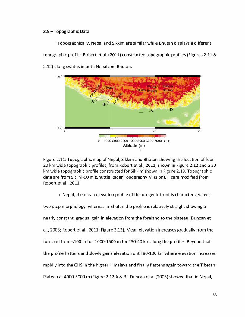
Topographically, Nepal and Sikkim are similar while Bhutan displays a different
topographic profile. Robert et al. (2011) constructed topographic profiles (Figures 2.11 &
2.12) along swaths in both Nepal and Bhutan.
Figure 2.11: Topographic map of Nepal, Sikkim and Bhutan showing the location of four 20 km wide topographic profiles, from Robert et al., 2011, shown in Figure 2.12 and a 50 km wide topographic profile constructed for Sikkim shown in Figure 2.13. Topographic data are from SRTM-90 m (Shuttle Radar Topography Mission). Figure modified from Robert et al., 2011.
In Nepal, the mean elevation profile of the orogenic front is characterized by a
two-step morphology, whereas in Bhutan the profile is relatively straight showing a
nearly constant, gradual gain in elevation from the foreland to the plateau (Duncan et
al., 2003; Robert et al., 2011; Figure 2.12). Mean elevation increases gradually from the
foreland from <100 m to ~1000-1500 m for ~30-40 km along the profiles. Beyond that
the profile flattens and slowly gains elevation until 80-100 km where elevation increases
rapidly into the GHS in the higher Himalaya and finally flattens again toward the Tibetan
Plateau at 4000-5000 m (Figure 2.12 A & B). Duncan et al (2003) showed that in Nepal,
33
areas with high topography and significant relief correlate with the surface exposure of
the GHS thrust sheet. In Nepal, the GHS is exposed in two bands: one ~20 km wide band
in northern Nepal at approximately 120-140 km along the profile (Figure 2.12 A & B) and
a narrower ~10 km wide band to the south that coincides with a southern zone of
moderate relief at ~30-40 km (2.12 B).
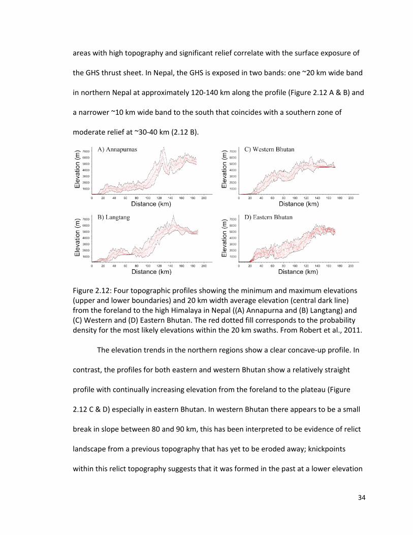
Figure 2.12: Four topographic profiles showing the minimum and maximum elevations (upper and lower boundaries) and 20 km width average elevation (central dark line) from the foreland to the high Himalaya in Nepal ((A) Annapurna and (B) Langtang) and (C) Western and (D) Eastern Bhutan. The red dotted fill corresponds to the probability density for the most likely elevations within the 20 km swaths. From Robert et al., 2011.
The elevation trends in the northern regions show a clear concave-up profile. In
contrast, the profiles for both eastern and western Bhutan show a relatively straight
profile with continually increasing elevation from the foreland to the plateau (Figure
2.12 C & D) especially in eastern Bhutan. In western Bhutan there appears to be a small
break in slope between 80 and 90 km, this has been interpreted to be evidence of relict
landscape from a previous topography that has yet to be eroded away; knickpoints
within this relict topography suggests that it was formed in the past at a lower elevation
34
and was then subsequently uplifted to its current position (Duncan et al., 2003; Grujic et
al., 2006). Bhutan profiles appear somewhat concave-up in the west and nearly straight
in the east, suggesting a more consistent gradual increase in elevation compared to the
sharp topographic break observed in Nepal. In addition, the GHS in Bhutan extends
further south and is composed of a much larger contiguous package, unbroken by
windows of LHS, compared to the two major bands of GHS in Nepal. The Bhutan range
shows a more consistent pattern of higher relief which correlates well with the location
of the GHS (Duncan et al., 2003).
In Sikkim (Figure 2.13), the DEM shows very clearly that the Rangit and Tista
windows coincide with low elevations flanking the major valleys of the Rangit and Tista
rivers. Elevations above 4 km appear to correlate generally with the boundaries of the
Tista window and the exposure of the GHS. The swath profile (Figure 2.14) indicates that
Sikkim also shows a poorly defined two-step north-south topographic profile with
isolated patches of high relief. Average elevation increases slowly from the foreland to a
first peak at ~27 °N and an elevation of ~1200-1300 m, and then declines in the area of
the Rangit Window into a slight ~ 100 m depression. Towards the northern edge of the
Tista Window, average elevation increases steadily up into the GHS to ~3000 m. Another
decrease in average elevation appears just to the north of the Tista Window, where the
Tista River is fed by two smaller rivers with valleys oriented in an east-west direction
(Figure 2.13). Then, elevation continues to increase steadily northward to an average
elevation of 5000-6000 m.
35

Figure 2.13: Digital Elevation Model of Sikkim between 26.5 °N - 28 °N and 88 °E - 89 °E constructed from SRTM (Shuttle Radar Topography Mission) 90 m data (http://srtm.csi.cgiar.org/). Structures are from Grujic et al., 2011 (same legend and abbreviations as in Figure 2.1). The shade grey rectangle shows the locations of a 50 km wide swath profile where elevation data were extracted and are presented in Figure 2.14. Blue lines indicate the location of the Rangit and Tista rivers.
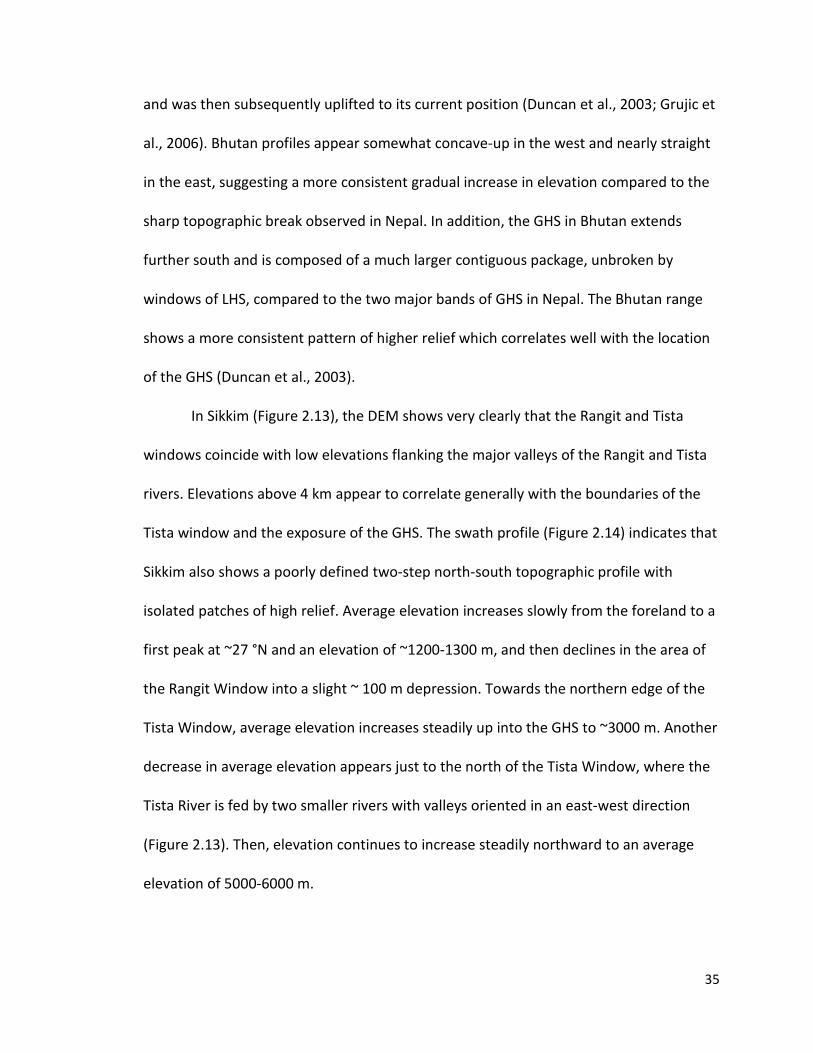
The minimum elevation curve shows a clear topographic break between 27.5 -
27.6 °N which is the approximate location of the northern boundary of the Tista Window
36
and the first appearance of the GHS. The overall topographic pattern of Sikkim seems to
be similar to the two-step morphology observed in Nepal.
Figure 2.14: A swath profile constructed along the profile indicated in Figure 2.10. Average elevation (center), maximum elevation (top) and minimum elevation (bottom) over the 50 km wide zone are plotted against distance north along the profile shown in Figure 2.11 at a ~93 m DEM sample interval. Red dots show the most common elevation at each point along the profile. Constructed from SRTM (Shuttle Radar Topography Mission) 90 m data (http://srtm.csi.cgiar.org/).
37
Chapter 3 - Thermochronology Methods and Results
3.1 - Introduction
To quantify late Tertiary upper crustal exhumation rates and constrain the
processes driving them along the Himalayan range front in Sikkim (India), a
multidisciplinary approach is used involving: 1) (U-Th)/He thermochronology on zircon
(e.g., Reiners, 2005), and 2) three-dimensional, forward and inverse thermokinematic
modelling using the software Pecube (Braun, 2003; Braun et al., 2012).
Eighteen in situ bedrock samples were collected along a NW-SE transect across the main
Himalayan structures, perpendicular to the range front and across the Rangit window
(Figure 3.1; see Appendix A for sample details). Zircons extracted from these samples
were analyzed using the (U-Th)/He method to produce single-grain cooling ages. These
cooling ages were then used as input, along with other thermal and material properties
and kinematic parameters, to construct forward and inverse models in order to test
different tectonic hypotheses and define a tectonic model that is the most compatible
with the data. This chapter will describe the (U-Th/He) methodology and the cooling
ages that were obtained from the samples. The model is described in Chapter 4.
3.2 - Zircon (U-Th)/He Thermochronology: Principles of the Method
Thermochronology is used to constrain the thermal histories of crustal rocks.
Many thermochronological methods (such as U-Th/He and 40Ar/39Ar) are based on the
radioactive decay of different parent radioisotopes into daughter products at
predictable rates. The daughter products are retained within a given mineral when it has
38
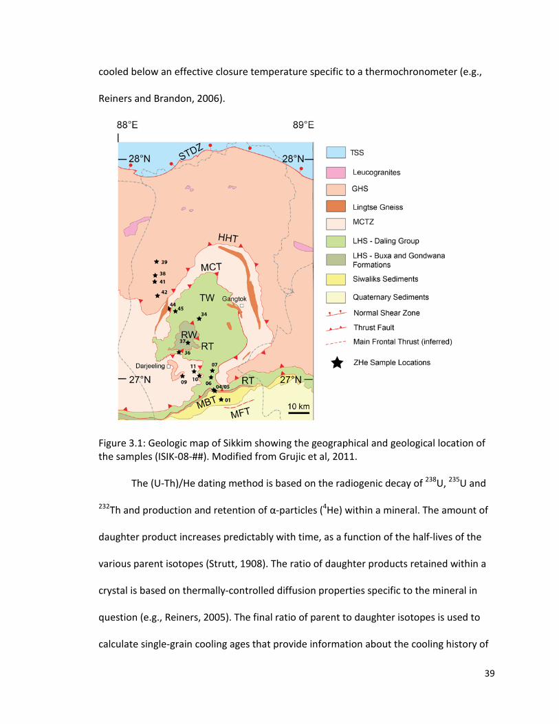
cooled below an effective closure temperature specific to a thermochronometer (e.g.,
Reiners and Brandon, 2006).
Figure 3.1: Geologic map of Sikkim showing the geographical and geological location of the samples (ISIK-08-##). Modified from Grujic et al, 2011.
The (U-Th)/He dating method is based on the radiogenic decay of 238U, 235U and
232Th and production and retention of α-particles (4He) within a mineral. The amount of
daughter product increases predictably with time, as a function of the half-lives of the
various parent isotopes (Strutt, 1908). The ratio of daughter products retained within a
crystal is based on thermally-controlled diffusion properties specific to the mineral in
question (e.g., Reiners, 2005). The final ratio of parent to daughter isotopes is used to
calculate single-grain cooling ages that provide information about the cooling history of
39

a mineral. Because they contain U and Th, zircon and apatite crystals are commonly used
in the (U-Th)/He technique (ZHe and AHe, respectively; Farley, 2002).
3.2.1 - Thermochronology
(U-Th)/He thermochronology is primarily used to constrain the thermal histories
of rocks residing in the upper crust by extracting cooling ages from certain minerals (e.g.,
apatite, zircon). Cooling ages represent the amount of time taken for a rock particle to
cool from its closure temperature along its exhumation pathway to the surface (Reiners,
2005). These cooling ages can be used, along with known or hypothesized thermal and
kinematic properties of the crust such as the radiogenic heat production rate and the
slip rate along faults, as constraints for reconstructing the time-temperature path of a
sample using thermo-kinematic Modelling.
In contractional settings, material in the hanging wall of a thrust fault is uplifted
on top of the footwall, generating stacks of crustal material (Figure 3.2; Stüwe and Barr,
1998). In order for any point in the thrust sheet to be exposed at the surface (and
become exhumed), erosion needs to remove the overlying material. The vertical
component of the particle path to the surface is known as exhumation. England and
Molnar (1990) defined the rate of crustal exhumation as being equal to the rate of
surface uplift subtracted from the rate of vertical rock uplift. In an orogenic setting
where thrust faulting is the primary tectonic control on the transport of crustal material,
the rate of exhumation is effectively equal to the rate of erosion.
40
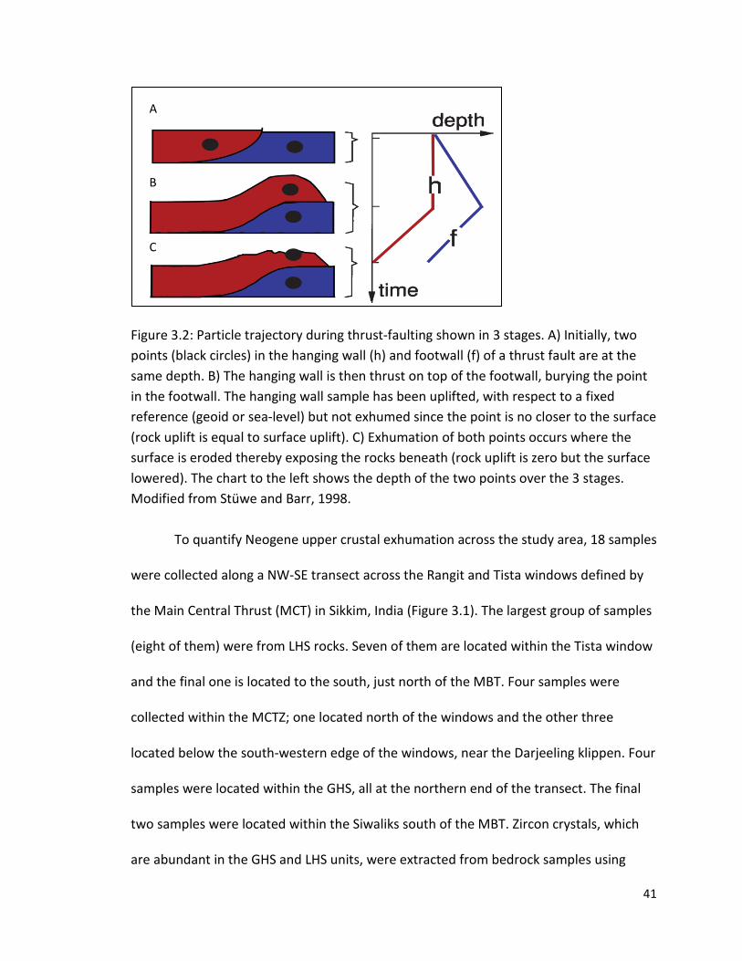
Figure 3.2: Particle trajectory during thrust-faulting shown in 3 stages. A) Initially, two points (black circles) in the hanging wall (h) and footwall (f) of a thrust fault are at the same depth. B) The hanging wall is then thrust on top of the footwall, burying the point in the footwall. The hanging wall sample has been uplifted, with respect to a fixed reference (geoid or sea-level) but not exhumed since the point is no closer to the surface (rock uplift is equal to surface uplift). C) Exhumation of both points occurs where the surface is eroded thereby exposing the rocks beneath (rock uplift is zero but the surface lowered). The chart to the left shows the depth of the two points over the 3 stages. Modified from Stüwe and Barr, 1998.
To quantify Neogene upper crustal exhumation across the study area, 18 samples
were collected along a NW-SE transect across the Rangit and Tista windows defined by
the Main Central Thrust (MCT) in Sikkim, India (Figure 3.1). The largest group of samples
(eight of them) were from LHS rocks. Seven of them are located within the Tista window
and the final one is located to the south, just north of the MBT. Four samples were
collected within the MCTZ; one located north of the windows and the other three
located below the south-western edge of the windows, near the Darjeeling klippen. Four
samples were located within the GHS, all at the northern end of the transect. The final
two samples were located within the Siwaliks south of the MBT. Zircon crystals, which
are abundant in the GHS and LHS units, were extracted from bedrock samples using
A
B
C
41
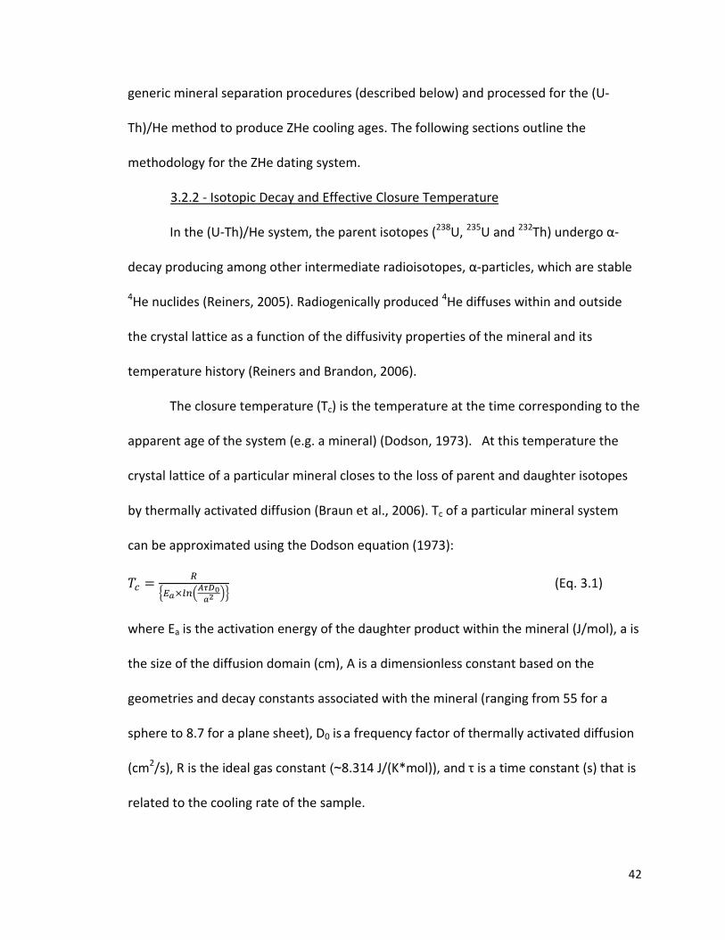
generic mineral separation procedures (described below) and processed for the (U-
Th)/He method to produce ZHe cooling ages. The following sections outline the
methodology for the ZHe dating system.
3.2.2 - Isotopic Decay and Effective Closure Temperature
In the (U-Th)/He system, the parent isotopes (238U, 235U and 232Th) undergo -
-particles, which are stable
4He nuclides (Reiners, 2005). Radiogenically produced 4He diffuses within and outside
the crystal lattice as a function of the diffusivity properties of the mineral and its
temperature history (Reiners and Brandon, 2006).
The closure temperature (Tc) is the temperature at the time corresponding to the
apparent age of the system (e.g. a mineral) (Dodson, 1973). At this temperature the
crystal lattice of a particular mineral closes to the loss of parent and daughter isotopes
by thermally activated diffusion (Braun et al., 2006). Tc of a particular mineral system
can be approximated using the Dodson equation (1973): = × (Eq. 3.1)
where Ea is the activation energy of the daughter product within the mineral (J/mol), a is
the size of the diffusion domain (cm), A is a dimensionless constant based on the
geometries and decay constants associated with the mineral (ranging from 55 for a
sphere to 8.7 for a plane sheet), D0 is a frequency factor of thermally activated diffusion
(cm2/s), R is the ideal gas constant 8.314 J/(K*mol)) (s) that is
related to the cooling rate of the sample.
42
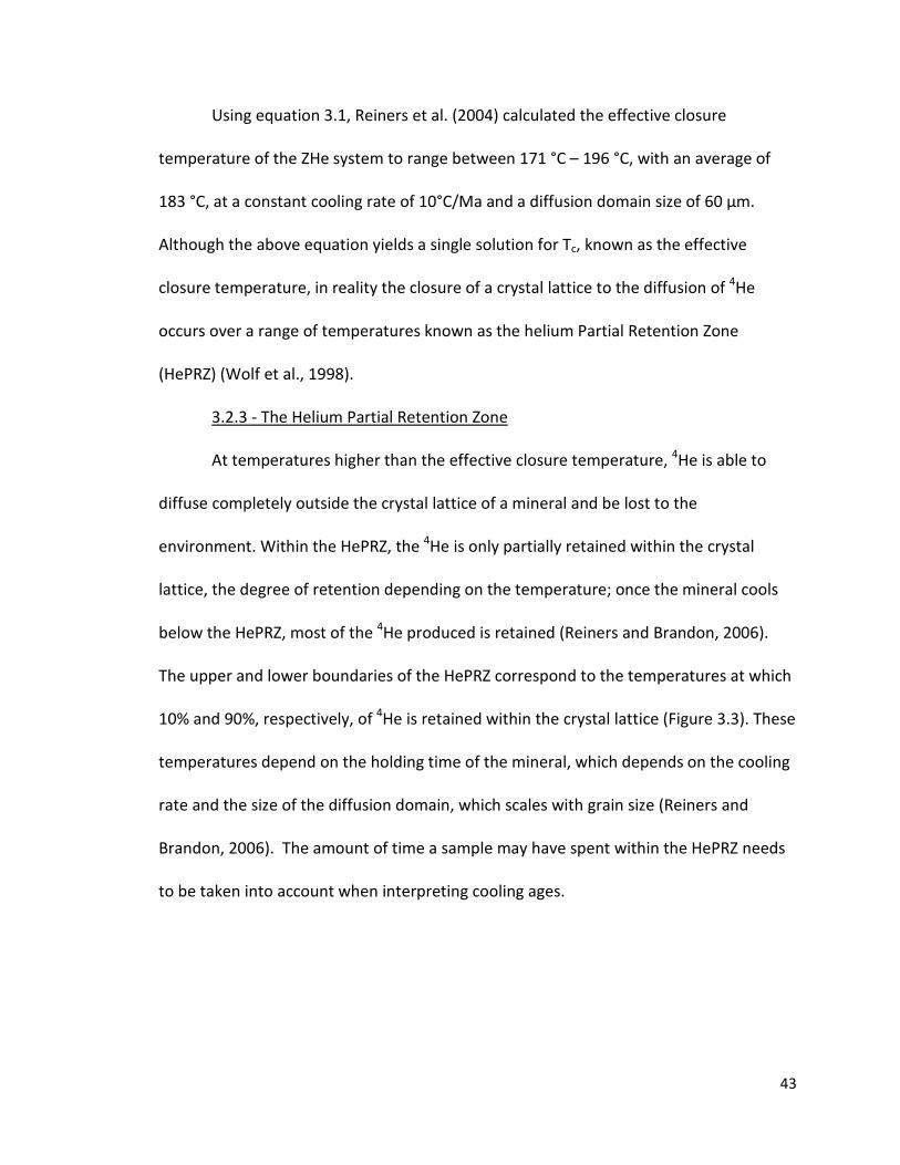
Using equation 3.1, Reiners et al. (2004) calculated the effective closure
temperature of the ZHe system to range between 171 °C – 196 °C, with an average of
183 °C, at a constant cooling rate of 10°C/Ma and a diffusion domain size of 60 µm.
Although the above equation yields a single solution for Tc, known as the effective
closure temperature, in reality the closure of a crystal lattice to the diffusion of 4He
occurs over a range of temperatures known as the helium Partial Retention Zone
(HePRZ) (Wolf et al., 1998).
3.2.3 - The Helium Partial Retention Zone
At temperatures higher than the effective closure temperature, 4He is able to
diffuse completely outside the crystal lattice of a mineral and be lost to the
environment. Within the HePRZ, the 4He is only partially retained within the crystal
lattice, the degree of retention depending on the temperature; once the mineral cools
below the HePRZ, most of the 4He produced is retained (Reiners and Brandon, 2006).
The upper and lower boundaries of the HePRZ correspond to the temperatures at which
10% and 90%, respectively, of 4He is retained within the crystal lattice (Figure 3.3). These
temperatures depend on the holding time of the mineral, which depends on the cooling
rate and the size of the diffusion domain, which scales with grain size (Reiners and
Brandon, 2006). The amount of time a sample may have spent within the HePRZ needs
to be taken into account when interpreting cooling ages.
43
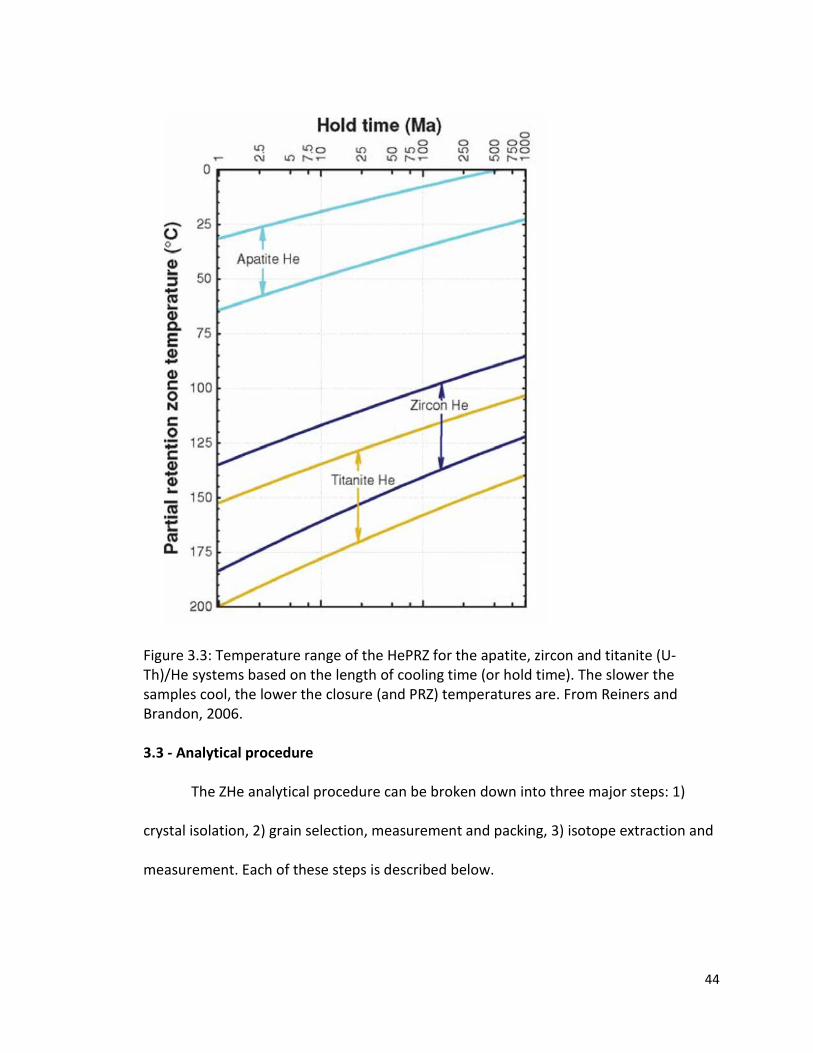
Figure 3.3: Temperature range of the HePRZ for the apatite, zircon and titanite (U-Th)/He systems based on the length of cooling time (or hold time). The slower the samples cool, the lower the closure (and PRZ) temperatures are. From Reiners and Brandon, 2006. 3.3 - Analytical procedure
The ZHe analytical procedure can be broken down into three major steps: 1)
crystal isolation, 2) grain selection, measurement and packing, 3) isotope extraction and
measurement. Each of these steps is described below.
44
3.3.1 - Crystal Isolation
The rock samples were each processed through a jaw crusher and then a disk mill
to a grain size of < 425 µm. The fractions were then taken to the Wilfley table where a
first relative density-based separation was done. The densest fractions containing the
mineral of interest were then immersed in sodium polytungstate (SPT), a heavy liquid
with a density of ~2.8 g/cm3, in order to separate the heavier minerals, such as zircon
(ρ~4.6 g/cm3) and apatite (ρ~3.2 g/cm3), from lighter constituents such as quartz and
feldspars (ρ≤2.7 g/cm3). The SPT heavy fractions were then processed through a Frantz
magnetic separator in order to remove magnetically susceptible minerals such as
metallic oxides and some micas (e.g., biotite). The final step involved immersion in a
second heavy liquid, diiodomethane (MI, ρ~3.2 g/cm3) in order to separate out minerals
such as apatite and concentrate the zircons. The heavy fractions were then inspected
under a stereoscopic microscope in order to select the zircons suitable for (U-Th)/He
dating.
3.3.2 - Grain Selection
Zircon grains were selected on the basis of size and crystal geometry with a
preference for grains that were large (see specifics below), euhedral, and free of mineral
inclusions (Reiners, 2005). Grain selection is a critical step in (U-Th)/He dating as the size
and geometry of the grains are directly related to the magnitude of the α-particle
ejection correction, explained below in section 3.5.2. Grains were examined using a
transmitted light stereoscopic microscope at magnification of x106 under both plane-
polarized light, for general selection, and cross-polarized light, for identification of
45

inclusions and/or fractures. Inclusions are undesirable as they may be composed of solid
radiogenic minerals that may contaminate the main crystal and bias the final ZHe cooling
age. Fluid inclusions are also undesirable as they represent areas contained within the
volume of the crystal that likely do not produce alpha particles (if the fluid is water).
Fractures are undesirable as they may have acted as escape pathways for helium during
cooling of the host crystal, and it is difficult to determine when a particular fracture was
created. Generally, the zircon grains selected for this study range from ~65-150 µm in
width (e.g., Figure 3.4). Larger grains tended to be less euhedral (rectangular prisms with
two pyramidal terminations) or contained more inclusions, whereas smaller grains
would require very large α-corrections. Euhedral zircons were preferentially selected as
they allow a more accurate α-correction (e.g., Reiners, 2005). For each sample analyzed
(18 in total) five acceptable grains were selected for dating, except for one sample
where only three suitable grains were found. A total of 88 aliquots were dated in this
study.
Figure 3.4: Grain ISIK-08-38-1, a euhedral zircon typical in dimensions of the grains that were selected. Each grain is photographed twice: first to measure the two longest axes, X and Y in photo a) and a second time, rotated 90 degrees along the x-axis, in order to measure the 3rd axis, Z in photo b). The lengths of the pyramidal terminations were also measured.
46
Each zircon crystal was photographed and measured before being wrapped in a 1
mm x 1 mm piece of platinum (Pt) foil. The measurements allow calculation of the
volume and surface area of each crystal, which are required to correct for loss of α-
particles due to crystal geometry. The Pt foil shields the grain from direct laser contact
and prevents shattering and/or uneven heating during 4He extraction.
3.4 - Isotope Extraction and Measurement
Extraction of parent and daughter isotopes was completed in two separate
phases, 1) non-destructive extraction of 4He at the Dalhousie Noble Gas Extraction
Laboratory and the Keck Isotope Laboratory at the University of California Santa Cruz
(UCSC) and 2) destructive 238U, 235U and 232Th measurement at UCSC.
3.4.1 - Laser Extraction and Measurement of Helium
4He extraction was completed for two sets of grains. The first set of 25 grains
(corresponding to five samples) was analyzed at Dalhousie while the remaining samples
were analyzed at UCSC due to time constraints. The samples, enclosed within Pt foil and
placed on a small planchet within a vacuum sealed chamber, were heated in sequence
at 1300 °C for 30 minutes at the Dalhousie line and 1250 °C in several 10 minute
intervals at UCSC, in order to extract all the helium trapped within each grain. This
difference in procedure is due to the different metals used to wrap the grains at each
lab. Platinum is the standard at Dalhousie while niobium is used at UCSC. Since platinum
had already been used to cover all the samples in this case, the laser at UCSC was
calibrated to compensate for the use of Pt foil. Meanwhile a pressure line attached to
the planchet was voided to a high vacuum (~10-8 torr) and then injected with a
47

manometrically calibrated amount of 3He spike (0.1 - 1 pmol), which was allowed to
equilibrate within the line. In our procedure, a spike is a liquid solution that carries a
known amount of two isotopes, one of which is a radioactive isotope that is being
analysed and the other a stable isotope of the same element that is enriched in
proportion to the other. The 4He extracted from the sample was then introduced to the
pressure line where it equilibrated with the spike and was then introduced into the mass
spectrometer for measurement. For each grain, 4He/3He ratios were measured over 30
cycles in order to obtain a mean ratio. The process was then repeated a second time to
extract any remaining 4He within the grain. If the re-extracted quantity of gas was > 2.5
% of the gas extracted during the initial extraction, then the crystal had to be heated and
analyzed a third time to release any remaining 4He that was not extracted from the grain
during the initial run. The procedure was repeated until the amount of gas extracted was
less than 2.5% of the total ratio. For most samples, a single re-extraction run was
sufficient. At UCSC, to test analytical precision, a line blank, cold blank, hot blank and
4He standard were analyzed between every five extractions. A line blank is a
measurement taken with no sample or spiked gases added to the He line and with the
extraction laser off. This is to ensure that no helium or other anomalous gases are
initially present within the line. A cold blank uses a similar process but in addition, an
empty platinum foil is placed on the sample planchet. A hot blank uses an empty
platinum foil but in this case, the foil is heated using the extraction laser in order to
confirm that no appreciable amount of helium is extracted from the foils. Both the cold
and hot blanks should produce little or no helium above the level found in the line blank.
48
For a properly functioning helium line, the amount of gas extracted during these blank
runs should be several orders of magnitude less than would be extracted from a sample.
Using the analyzed 4He/3He ratio, the amount of spike added and the ratio of 4He/3He
with a calibrated 4He standard, the amount of 4He extracted from each single grain was
calculated. This is explained below in Section 3.4.4.
3.4.2 - Extraction of U and Th Isotopes
Parent isotope extraction was achieved through sample dissolution and
introduction to an inductively coupled plasma mass spectrometer (ICP-MS). After 4He
extraction and measurement, the zircons were removed from the Pt foils because
dissolved Pt and the argon plasma used within the ICP-MS may interfere with isotope
measurement by producing PtAr molecules that have an atomic weight of ~235 amu,
nearly identical to that of 235U, one of the parent isotopes. The ICP-MS is unable to
discriminate between 235U and PtAr so the U concentration measured may be biased.
Once removed from their foils, the zircons were placed into Teflon tubes and mixed with
50 µm of spike solution comprising 7.55 ± 0.10 ng/ml 236U and 12.3 ± 0.10 ng/ml 229Th.
3.4.3 - Dissolution of the Zircons
Finally, a 1:8 ratio of hydrofluoric acid (HF) and nitric acid (HNO3) was added to
each tube. Dissolution of the samples was aided by the use of high-pressure digestion
vessels (also known as Parr bombs) which were placed in an oven at ~220 °C for ~72
hours to ensure full dissolution. Once removed from the bombs, the contents of each
Teflon vial were transferred to a larger vial and introduced to a high-resolution (single-
collector) Element-2 ICP-MS, which measured the ratios of natural isotopes (238U and
49
232Th) to spike isotopes (236U and 229Th). The ratios were used to calculate the
concentration of natural isotopes using the isotope dilution technique (see section 2.5.4
below). Several spiked and acid blanks were analyzed concurrently with the samples in
order to test the analytical precision.
3.4.4 - Isotope Dilution Technique and Calculations
Isotope dilution is a technique used to calculate the amount of a specific
radioisotope in a sample based on the natural isotope ratio (e.g., 238U/235U) and a known
isotope ratio contained in a spike solution (e.g., 238U/236U), which is dissolved within and
mixed with the sample prior to ICP-MS analysis. The mass of a specific radioisotope in a
spiked solution can be calculated according to Atterdorn and Bowen (1998):
NW = SW �WNWS� �AbS
A−RM∗AbSB
RM∗AbNB−AbN
A� (Eq. 3.2)
where Nw and Sw are the masses of the natural isotope A (e.g., 238U) and spike isotope B
(e.g., 236U), respectively, WN and Ws are the isotopic weights of the natural isotope and
spike isotope, 𝐴𝑏𝑆𝐴, 𝐴𝑏𝑆𝐵, 𝐴𝑏𝑁𝐵 and 𝐴𝑏𝑁𝐴 are the relative abundances of isotopes A and B
in the spike and in nature, and RM is the ratio of isotopes A and B obtained through ICP-
MS analysis. Solving for Nw yields a mass of the isotope of interest, which can then be
converted into a concentration by dividing Nw by the mass of the zircon grain being
analyzed. To solve the age equations, the number of moles of the isotope(s) of interest
is needed, and so Nw is divided by the molar mass of the specific isotope to obtain its
molar concentration.
50

3.5 - Age Calculation and Alpha-Ejection Correction
3.5.1 - U-Th/He Age Calculation
Once the concentrations of parent and daughter isotopes are known, the values
are used to calculate the cooling age of the sample. The cooling age, t, is calculated using
the following helium ingrowth equation (Farley, 2002):
𝐻𝑒4 = 8[ 𝑈] 238 �𝑒(𝜆238𝑡) − 1� + 7[ 𝑈] � 1
137.88�
238 �𝑒(𝜆235𝑡) − 1� + 6[ 𝑇ℎ 232 ]�𝑒(𝜆232𝑡)1�
(Eq. 3.3)
where [x] represents the concentration of a particular isotope (4He, 238U, 235U or 232Th), λ
is the decay constant of a particular isotope and t is the uncorrected cooling age. 4He is
the product of the decay of several different isotopes. For each atom of 238U (λ=1.55e-10
years), 235U (λ=9.85e-10 years) and 232Th (λ=4.95e-11 years) that undergoes decay, eight,
seven and six 4He atoms are produced respectively. The cooling age cannot, however, be
calculated directly using this equation since the variable t is present a number of times
within the equation and cannot be isolated. There are several solutions to this problem;
three of these are outlined below and their results for a single ZHe sample compared.
Linear Approximation
The simplest solution is a linear approximation of the cooling age of the sample,
which is reasonably accurate when cooling ages are young (t<<1/λ235U) (Veermesch,
2008). For this solution, the present day 4He production rate (P) is calculated according
to (Veermesch, 2008):
𝑃 = 8[ 𝑈] �137.88138.88
� 238 𝜆238 + 7[ 𝑈]
238 � 1138.88
� 𝜆235 + 6[ 𝑇ℎ
232 ]𝜆232 (Eq. 3.4)
51
Once P is calculated, t can be calculated using the simple equation:
𝑡 = � 𝐻𝑒 4 �𝑃
(Eq. 3.5)
where t is an uncorrected approximation of the cooling age of the sample.
Indirect iterative method
The second solution is the most commonly used, but also the most complex. For
this iterative solution the cooling age t is calculated using a Taylor Series approximation
of equation 3.3. A Taylor Series approximates of a function as a sum of terms calculated
from the values of its derivatives at a single point. To the first derivative, the solution is
(M. G. Fellin, personal communication):
𝐻𝑒 4 ≈
�8[ 𝑈] �137.88138.88
� 238 �𝑒(𝜆238𝑡0) − 1� + 7 �
� 𝑈 238 �
138.88�
�𝑒(𝜆235𝑡0) − 1� + 6[ 𝑇ℎ]
232 �𝑒(𝜆232𝑡0) −
1�� + (𝑡1 − 𝑡0) �8[ 𝑈] �137.88138.88
� 238 �𝜆238𝑒(𝜆238𝑡0)� + 7[ 𝑈] � 1
138.88�
238 �𝜆235𝑒(𝜆235𝑡0)� +
6[ 𝑇ℎ 232 ]�𝜆232𝑒(𝜆232𝑡0)�� (Eq.3.6)
where the first term is approximated to be ƒ(t0) and the third term to be ƒ’(t0).
Rearranging the equation to solve for t1, the equation reduces to:
𝑡1 ≈𝐻𝑒 4 −𝑓(𝑡0)+𝑡0𝑓′(𝑡0)
𝑓′(𝑡0) (Eq. 3.7)
where t0 is an initial estimate of the age of the sample and t1 is the approximate
calculated age of the sample. To solve the equation for t1, an estimate of the cooling age
must be made and substituted to the variable t0. To test whether t1 is an accurate value
for the sample cooling age, the relative error between t1 and t0 must be calculated
according to:
52
𝐸𝑎 = 𝑡1−𝑡0𝑡1
× 100 (Eq. 3.8)
If the error is greater than ~5%, the equation must be re-iterated a second time. The
new t1 substitutes for the previously estimated t0, and the equation is solved again for a
t2. The error is then re-calculated. This procedure is repeated until the relative error
between tn and tn+1 is < 5%. Once the error is sufficiently low, the tn calculated is the
uncorrected cooling age of the sample. This is likely the most accurate solution, but it is
also the most computationally intensive.
Direct non-iterative method
The third solution is a non-iterative approximation from Meesters and Dunai
(2005) that is less accurate within a small percentage of error when compared to the
iterative solution but requires less calculation. The solution involves calculating a total
cumulative 4He production value, P, such that:
𝑃1 = 8𝜆238[ 𝑈] 238 𝑃2 = 7𝜆235[ 𝑈]
235 𝑃3 = 6𝜆232[ 𝑇ℎ] 232 (Eq. 3.9)
𝑃 = 𝑃1 + 𝑃2 + 𝑃3 (Eq. 3.10)
A weighted mean decay rate, λwm, must also be calculated, using the various isotope
production rates as a weighting mechanism:
λwm = ∑ PjλjPj (Eq. 3.11)
With this value, the approximate age, tapp, can be calculated according to:
𝑡𝑎𝑝𝑝 = 1𝜆𝑤𝑚
𝑙𝑛 �𝜆𝑤𝑚𝑃
[ 𝐻𝑒 4 ] + 1� (Eq. 3.12)
53
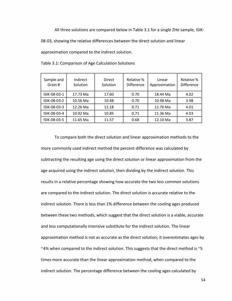
All three solutions are compared below in Table 3.1 for a single ZHe sample, ISIK-
08-03, showing the relative differences between the direct solution and linear
approximation compared to the indirect solution.
Table 3.1: Comparison of Age Calculation Solutions
Sample and Grain #
Indirect Solution
Direct Solution
Relative % Difference
Linear Approximation
Relative % Difference
ISIK-08-03-1 17.73 Ma 17.60 0.70 18.44 Ma 4.02 ISIK-08-03-2 10.56 Ma 10.48 0.70 10.98 Ma 3.98 ISIK-08-03-3 12.26 Ma 12.18 0.71 12.76 Ma 4.01 ISIK-08-03-4 10.92 Ma 10.85 0.71 11.36 Ma 4.03 ISIK-08-03-5 11.65 Ma 11.57 0.68 12.10 Ma 3.87
To compare both the direct solution and linear approximation methods to the
more commonly used indirect method the percent difference was calculated by
subtracting the resulting age using the direct solution or linear approximation from the
age acquired using the indirect solution, then dividing by the indirect solution. This
results in a relative percentage showing how accurate the two less common solutions
are compared to the indirect solution. The direct solution is accurate relative to the
indirect solution. There is less than 1% difference between the cooling ages produced
between these two methods, which suggest that the direct solution is a viable, accurate
and less computationally intensive substitute for the indirect solution. The linear
approximation method is not as accurate as the direct solution; it overestimates ages by
~4% when compared to the indirect solution. This suggests that the direct method is ~5
times more accurate than the linear approximation method, when compared to the
indirect solution. The percentage difference between the cooling ages calculated by
54

direct and indirect methods results in a difference in age that is far less than the age
uncertainty between grains from the same sample. For this study, the indirect method is
used as it is the most accurate and accepted solution.
3.5.2 - Alpha-Ejection Correction
The cooling ages are a product of the ratio of parent and daughter isotopes
measured within the samples; however, these values need to be corrected for the
ejection of 4He (α-particles) during nuclear decay (Farley et al., 1996). During α-decay,
the parent isotopes (e.g., 238U) release a certain amount of kinetic energy, ejecting the
produced α-particles a certain distance from the site of decay (Figure 3.5), depending on
the medium. In the case of zircon, this distance is ~17-20 µm, depending on which
isotope is undergoing decay (Farley et al, 1996). Consequently, there is a proportion of
α-particles produced within 20 µm of the edge of the zircon grain that will be ejected
from the grain and subsequently lost to the environment. The probability of ejection
depends on both the distance to the edge of the grain from the site of decay and the
geometry of the grain itself. This process biases the final 4He concentration in the grain
because some of the 4He that has been produced is lost to the environment, even
though the parent isotopes are still present in the grain. This results in an
underestimation of the “true” age of the sample. Depending on the size, shape and age
of the grain, this underestimation can be significant and must be corrected for.
55
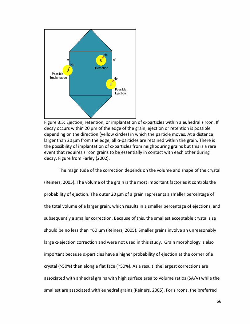
Figure 3.5: Ejection, retention, or implantation of α-particles within a euhedral zircon. If decay occurs within 20 µm of the edge of the grain, ejection or retention is possible depending on the direction (yellow circles) in which the particle moves. At a distance larger than 20 µm from the edge, all α-particles are retained within the grain. There is the possibility of implantation of α-particles from neighbouring grains but this is a rare event that requires zircon grains to be essentially in contact with each other during decay. Figure from Farley (2002).
The magnitude of the correction depends on the volume and shape of the crystal
(Reiners, 2005). The volume of the grain is the most important factor as it controls the
probability of ejection. The outer 20 µm of a grain represents a smaller percentage of
the total volume of a larger grain, which results in a smaller percentage of ejections, and
subsequently a smaller correction. Because of this, the smallest acceptable crystal size
should be no less than ~60 µm (Reiners, 2005). Smaller grains involve an unreasonably
large α-ejection correction and were not used in this study. Grain morphology is also
important because α-particles have a higher probability of ejection at the corner of a
crystal (>50%) than along a flat face (~50%). As a result, the largest corrections are
associated with anhedral grains with high surface area to volume ratios (SA/V) while the
smallest are associated with euhedral grains (Reiners, 2005). For zircons, the preferred
56
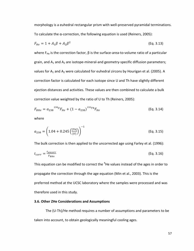
morphology is a euhedral rectangular prism with well-preserved pyramidal terminations.
To calculate the α-correction, the following equation is used (Reiners, 2005):
𝐹𝐻𝑒 = 1 + 𝐴1𝛽 + 𝐴2𝛽2 (Eq. 3.13)
where FHe is the correction factor, β is the surface-area-to-volume ratio of a particular
grain, and A1 and A2 are isotope-mineral-and geometry-specific diffusion parameters;
values for A1 and A2 were calculated for euhedral zircons by Hourigan et al. (2005). A
correction factor is calculated for each isotope since U and Th have slightly different
ejection distances and activities. These values are then combined to calculate a bulk
correction value weighted by the ratio of U to Th (Reiners, 2005):
𝐹𝐵𝐻𝑒 = 𝑎238 𝐹 𝑈 238
𝐻𝑒 + (1 − 𝑎238) 𝐹 𝑇ℎ 232
𝐻𝑒 (Eq. 3.14)
where
𝑎238 = �1.04 + 0.245 �[𝑇ℎ][𝑈]��
−1
(Eq. 3.15)
The bulk correction is then applied to the uncorrected age using Farley et al. (1996):
𝑡𝑐𝑜𝑟𝑟 = 𝑡𝑢𝑛𝑐𝑜𝑟𝑟𝐹𝐵𝐻𝑒
(Eq. 3.16)
This equation can be modified to correct the 4He values instead of the ages in order to
propagate the correction through the age equation (Min et al., 2003). This is the
preferred method at the UCSC laboratory where the samples were processed and was
therefore used in this study.
3.6. Other ZHe Considerations and Assumptions
The (U-Th)/He method requires a number of assumptions and parameters to be
taken into account, to obtain geologically meaningful cooling ages.
57

3.6.1 - Presence of Pre-Existing Helium
Pre-existing 4He in the crystals would bias the cooling ages by overestimating
them. The method assumes that the crystals do not initially contain 4He that would be
derived from geologic or atmospheric sources. This assumption is most likely valid in the
case of an atmospheric source because the concentration of 4He present in the Earth’s
atmosphere (~5ppm) is insignificant, as is the amount produced within the Earth (Farley,
2002).
3.6.2 - Secular Equilibrium
Secular equilibrium is a state that occurs when the production and the decay
rates of a particular radiogenic isotope become equal. It requires that the half-life of a
parent isotope is much larger than the half-life of its daughter isotope, thereby limiting
the radioactive decay of the daughter and eventually bringing the production rate of
various daughter isotopes into equilibrium with that of the parent isotope; the amount
of daughter isotope that undergoes decay is the same as the amount produced through
decay of the parent isotope over geologic time. Secular equilibrium of parent isotopes is
assumed so that the equation to calculate cooling age can be solved correctly (Farley,
2002). If equilibrium is not reached, Eq.3 becomes less accurate as the rate of decay of
parent isotopes into the final daughter isotope will be affected. This assumption is likely
valid as the half-lives of intermediate daughter products within the decay chains of
parent isotopes are relatively small as compared to the half-lives of the initial parent. For
example, 238U has a half-life of ~4.47 Ga, while the intermediate isotope within the 238U
decay chain with the longest half-life is 230Th with a half-life of ~77 ka; other
58
intermediate isotopes have half-lives on the scale of minutes to days. Thus, decay of
intermediate isotopes is approximately synchronous with the decay of their initial
parent. Farley (2002) pointed out that secular equilibrium is achieved (with respect to
the U and Th decay chains) for crystals older than 0.35 Ma.
3.6.3 - Zonation of Parent Isotopes
The zonation of parent isotopes within analyzed crystals poses significant
problems when applying the α-correction and may lead to over- or underestimates of
actual cooling ages (Hourigan et al, 2005). For example, if the core of a zircon is enriched
in parent isotopes as compared to its rim, fewer extra-crystal ejections of alpha particles
will occur because the bulk of parent isotopes is located further than one stopping
distance from the rim of the grain. It is assumed that the distribution of the parent
isotopes is homogeneous within the grain. No significant zonation was observed during
selection of the crystals used here, however this is based only on microscope inspection.
3.6.4 - Samarium (Sm)
In some cases, Sm may be a significant 4He producing parent isotope, for
example, for apatite crystals showing high Sm concentrations (e.g., the Durango apatite,
Reiners and Nicolescu, 2006). However, Sm only produces a single 4He particle through
its short decay chain, compared to 8, 7, and 6 for 238U, 235U and 232Th, respectively. In
addition, the half-life of Sm (~1.06 Ga) is very long so very few decays are likely to take
place unless the samples are very old. Despite this, the decay of Sm can contribute
significantly to 4He production in samples with a high Sm concentration. In contrast to
apatites, zircons tend to have lower Sm concentrations, which does not significantly
59
affect the cooling age of the zircon crystals (Reiners, 2005). With this in mind, the
contribution of Sm to α-particle production was not taken into account in this study. If
Sm was present in some of the zircon grains, our ZHe ages would overestimate the
cooling ages.
3.7 - ZHe Cooling Age Results
Eighteen samples of zircon were analyzed using U-Th/He thermochronology. For
data reproducibility five aliquots per sample were processed, except for sample ISIK-08-
36 where only three acceptable grains were found. Several samples contained outlier
data that were discarded due to anomalous U, Th or He concentrations. Single-grain
ages that were more than two standard deviations older or younger than the mean
cooling age of the sample they belonged to were discarded and the sample mean
recalculated with the remaining grains. The standard error was calculated for each
sample by dividing the population standard deviation by the square root of the number
of samples. Here we present the results of our ZHe thermochronology (Table 3.2).
3.7.1 - ZHe Cooling Age Descriptions
Of the 18 ZHe samples originally processed, 17 were selected for use in this
study. The samples produced late Miocene-Pliocene cooling ages ranging from 1.30 ±
0.03 Ma to 12.94 ± 1.05 Ma (Figure 3.6). The omitted sample, ISIK-08-04, yielded single-
grain ages ranging from 167 Ma to 355 Ma, indicating that this sample was not
completely reset or possibly had an inclusion that was not detected. The results are
shown in Table 3.2. Shown are the sample numbers, the amount of parent and daughter
isotopes in moles, the grain dimensions, the α-correction factor, the single grain 4He
60

corrected ages in Ma, mean sample age and the statistical error of this mean age. Data
shown in red were discarded.
Several aliquots were discarded on the basis of anomalous isotope values and
several others because of significantly too young or old ages compared to the rest of the
grains in their respective samples. A single aliquot was also lost during processing and
another did not contain helium and was discarded (ISIK-08-01-1). These aliquots are
shown in red in Table 3.2. Two Fish Canyon Tuff zircon standards were also analyzed at
UCSC for precision and returned uncorrected ages of 26.31±0.92 and 20.83±0.33. The
first standard returned an age slightly too old but the second was within error of the ~21
Ma (average) uncorrected age obtained by Reiners et al. (2004) using the (U-Th)/He
system.
Table 3.2: Zircon (U-Th)/He results.
μ
ISIK-08-01-1 N/A 0.77 N/A 12.94 1.05ISIK-08-01-2 5.03E-13 3.60E-11 2.61E-13 5.80E-12 10.44 0.80 12.83ISIK-08-01-3 1.59E-13 1.55E-11 1.13E-13 2.35E-12 7.63 0.72 10.25ISIK-08-01-4 1.65E-13 1.06E-11 7.71E-14 6.04E-13 11.89 0.71 16.16ISIK-08-01-5 6.30E-13 4.82E-11 3.49E-13 8.00E-13 10.08 0.79 12.50
ISIK-08-03-1 1.19E-13 7.48E-12 5.42E-14 7.57E-13 12.02 0.68 16.89 10.90 1.10ISIK-08-03-2 6.72E-13 6.55E-11 4.75E-13 6.21E-12 7.77 0.74 10.07ISIK-08-03-3 2.93E-13 2.56E-11 1.86E-13 1.92E-12 8.71 0.72 11.70ISIK-08-03-4 7.44E-13 6.97E-11 5.05E-13 3.60E-12 8.17 0.75 10.52ISIK-08-03-5 9.79E-14 8.69E-12 6.31E-14 1.98E-12 8.28 0.72 11.32
61
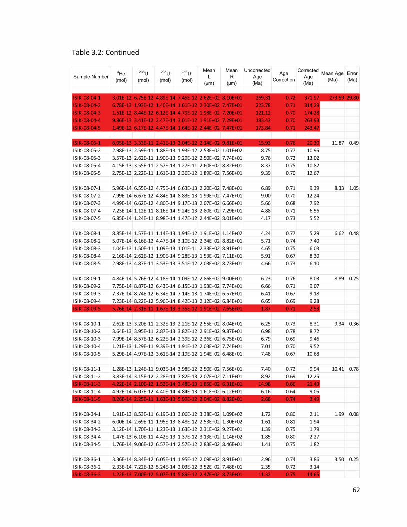
Table 3.2: Continued
μ
ISIK-08-04-1 3.01E-12 6.75E-12 4.89E-14 7.45E-12 269.31 0.72 371.97 273.59 29.80ISIK-08-04-2 6.78E-13 1.93E-12 1.40E-14 1.61E-12 223.78 0.71 314.29ISIK-08-04-3 1.51E-12 8.44E-12 6.12E-14 4.79E-12 121.12 0.70 174.28ISIK-08-04-4 9.86E-13 3.41E-12 2.47E-14 3.01E-12 183.43 0.70 263.93ISIK-08-04-5 1.49E-12 6.17E-12 4.47E-14 1.64E-12 173.84 0.71 243.47
ISIK-08-05-1 6.95E-13 3.33E-11 2.41E-13 2.04E-12 15.93 0.76 20.30 11.87 0.49ISIK-08-05-2 2.98E-13 2.59E-11 1.88E-13 1.93E-12 8.75 0.77 10.95ISIK-08-05-3 3.57E-13 2.62E-11 1.90E-13 9.29E-12 9.76 0.72 13.02ISIK-08-05-4 4.15E-13 3.55E-11 2.57E-13 1.27E-11 8.37 0.75 10.82ISIK-08-05-5 2.75E-13 2.22E-11 1.61E-13 2.36E-12 9.39 0.70 12.67
ISIK-08-07-1 5.96E-14 6.55E-12 4.75E-14 6.63E-13 6.89 0.71 9.39 8.33 1.05ISIK-08-07-2 7.99E-14 6.67E-12 4.84E-14 8.83E-13 9.00 0.70 12.24ISIK-08-07-3 4.99E-14 6.62E-12 4.80E-14 9.17E-13 5.66 0.68 7.92ISIK-08-07-4 7.23E-14 1.12E-11 8.16E-14 9.24E-13 4.88 0.71 6.56ISIK-08-07-5 6.85E-14 1.24E-11 8.98E-14 1.47E-12 4.17 0.73 5.52
ISIK-08-08-1 8.85E-14 1.57E-11 1.14E-13 1.94E-12 4.24 0.77 5.29 6.62 0.48ISIK-08-08-2 5.07E-14 6.16E-12 4.47E-14 3.10E-12 5.71 0.74 7.40ISIK-08-08-3 1.04E-13 1.50E-11 1.09E-13 1.01E-11 4.65 0.75 6.03ISIK-08-08-4 2.16E-14 2.62E-12 1.90E-14 9.28E-13 5.91 0.67 8.30ISIK-08-08-5 2.98E-13 4.87E-11 3.53E-13 3.51E-12 4.66 0.73 6.10
ISIK-08-09-1 4.84E-14 5.76E-12 4.18E-14 1.09E-12 6.23 0.76 8.03 8.89 0.25ISIK-08-09-2 7.75E-14 8.87E-12 6.43E-14 6.15E-13 6.66 0.71 9.07ISIK-08-09-3 7.37E-14 8.74E-12 6.34E-14 7.14E-13 6.41 0.67 9.18ISIK-08-09-4 7.23E-14 8.22E-12 5.96E-14 8.42E-13 6.65 0.69 9.28ISIK-08-09-5 5.76E-14 2.31E-11 1.67E-13 3.35E-12 1.87 0.71 2.53
ISIK-08-10-1 2.62E-13 3.20E-11 2.32E-13 2.21E-12 6.25 0.73 8.31 9.34 0.36ISIK-08-10-2 3.64E-13 3.95E-11 2.87E-13 3.82E-12 6.98 0.78 8.72ISIK-08-10-3 7.99E-14 8.57E-12 6.22E-14 2.39E-12 6.79 0.69 9.46ISIK-08-10-4 1.21E-13 1.29E-11 9.39E-14 1.91E-12 7.01 0.70 9.52ISIK-08-10-5 5.29E-14 4.97E-12 3.61E-14 2.19E-12 7.48 0.67 10.68
ISIK-08-11-1 1.28E-13 1.24E-11 9.03E-14 3.98E-12 7.40 0.72 9.94 10.41 0.78ISIK-08-11-2 3.83E-14 3.15E-12 2.28E-14 7.82E-13 8.92 0.69 12.25ISIK-08-11-3 4.22E-14 2.10E-12 1.52E-14 3.48E-13 14.98 0.66 21.43ISIK-08-11-4 4.92E-14 6.07E-12 4.40E-14 4.84E-13 6.16 0.64 9.05ISIK-08-11-5 8.26E-14 2.25E-11 1.63E-13 5.99E-12 2.68 0.74 3.49
ISIK-08-34-1 1.91E-13 8.53E-11 6.19E-13 3.06E-12 1.72 0.80 2.11 1.99 0.08ISIK-08-34-2 6.00E-14 2.69E-11 1.95E-13 8.48E-12 1.61 0.81 1.94ISIK-08-34-3 3.12E-14 1.70E-11 1.23E-13 1.63E-12 1.39 0.75 1.79ISIK-08-34-4 1.47E-13 6.10E-11 4.42E-13 1.37E-12 1.85 0.80 2.27ISIK-08-34-5 1.76E-14 9.06E-12 6.57E-14 2.57E-12 1.41 0.75 1.82
ISIK-08-36-1 3.36E-14 8.34E-12 6.05E-14 1.95E-12 2.96 0.74 3.86 3.50 0.25ISIK-08-36-2 2.33E-14 7.22E-12 5.24E-14 2.03E-12 2.35 0.72 3.14ISIK-08-36-3 1.22E-13 7.00E-12 5.07E-14 5.89E-12 11.32 0.75 14.65
62
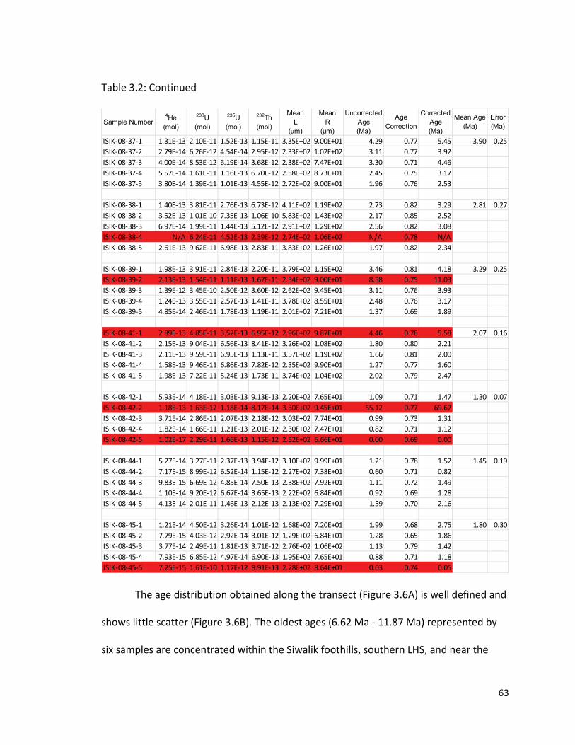
Table 3.2: Continued
The age distribution obtained along the transect (Figure 3.6A) is well defined and
shows little scatter (Figure 3.6B). The oldest ages (6.62 Ma - 11.87 Ma) represented by
six samples are concentrated within the Siwalik foothills, southern LHS, and near the
μISIK-08-37-1 1.31E-13 2.10E-11 1.52E-13 1.15E-11 4.29 0.77 5.45 3.90 0.25ISIK-08-37-2 2.79E-14 6.26E-12 4.54E-14 2.95E-12 3.11 0.77 3.92ISIK-08-37-3 4.00E-14 8.53E-12 6.19E-14 3.68E-12 3.30 0.71 4.46ISIK-08-37-4 5.57E-14 1.61E-11 1.16E-13 6.70E-12 2.45 0.75 3.17ISIK-08-37-5 3.80E-14 1.39E-11 1.01E-13 4.55E-12 1.96 0.76 2.53
ISIK-08-38-1 1.40E-13 3.81E-11 2.76E-13 6.73E-12 2.73 0.82 3.29 2.81 0.27ISIK-08-38-2 3.52E-13 1.01E-10 7.35E-13 1.06E-10 2.17 0.85 2.52ISIK-08-38-3 6.97E-14 1.99E-11 1.44E-13 5.12E-12 2.56 0.82 3.08ISIK-08-38-4 N/A 6.24E-11 4.52E-13 2.39E-12 N/A 0.78 N/AISIK-08-38-5 2.61E-13 9.62E-11 6.98E-13 2.83E-11 1.97 0.82 2.34
ISIK-08-39-1 1.98E-13 3.91E-11 2.84E-13 2.20E-11 3.46 0.81 4.18 3.29 0.25ISIK-08-39-2 2.13E-13 1.54E-11 1.11E-13 1.67E-11 8.58 0.75 11.03ISIK-08-39-3 1.39E-12 3.45E-10 2.50E-12 3.60E-12 3.11 0.76 3.93ISIK-08-39-4 1.24E-13 3.55E-11 2.57E-13 1.41E-11 2.48 0.76 3.17ISIK-08-39-5 4.85E-14 2.46E-11 1.78E-13 1.19E-11 1.37 0.69 1.89
ISIK-08-41-1 2.89E-13 4.85E-11 3.52E-13 6.95E-12 4.46 0.78 5.58 2.07 0.16ISIK-08-41-2 2.15E-13 9.04E-11 6.56E-13 8.41E-12 1.80 0.80 2.21ISIK-08-41-3 2.11E-13 9.59E-11 6.95E-13 1.13E-11 1.66 0.81 2.00ISIK-08-41-4 1.58E-13 9.46E-11 6.86E-13 7.82E-12 1.27 0.77 1.60ISIK-08-41-5 1.98E-13 7.22E-11 5.24E-13 1.73E-11 2.02 0.79 2.47
ISIK-08-42-1 5.93E-14 4.18E-11 3.03E-13 9.13E-13 1.09 0.71 1.47 1.30 0.07ISIK-08-42-2 1.18E-13 1.63E-12 1.18E-14 8.17E-14 55.12 0.77 69.67ISIK-08-42-3 3.71E-14 2.86E-11 2.07E-13 2.18E-12 0.99 0.73 1.31ISIK-08-42-4 1.82E-14 1.66E-11 1.21E-13 2.01E-12 0.82 0.71 1.12ISIK-08-42-5 1.02E-17 2.29E-11 1.66E-13 1.15E-12 0.00 0.69 0.00
ISIK-08-44-1 5.27E-14 3.27E-11 2.37E-13 3.94E-12 1.21 0.78 1.52 1.45 0.19ISIK-08-44-2 7.17E-15 8.99E-12 6.52E-14 1.15E-12 0.60 0.71 0.82ISIK-08-44-3 9.83E-15 6.69E-12 4.85E-14 7.50E-13 1.11 0.72 1.49ISIK-08-44-4 1.10E-14 9.20E-12 6.67E-14 3.65E-13 0.92 0.69 1.28ISIK-08-44-5 4.13E-14 2.01E-11 1.46E-13 2.12E-13 1.59 0.70 2.16
ISIK-08-45-1 1.21E-14 4.50E-12 3.26E-14 1.01E-12 1.99 0.68 2.75 1.80 0.30ISIK-08-45-2 7.79E-15 4.03E-12 2.92E-14 3.01E-12 1.28 0.65 1.86ISIK-08-45-3 3.77E-14 2.49E-11 1.81E-13 3.71E-12 1.13 0.79 1.42ISIK-08-45-4 7.93E-15 6.85E-12 4.97E-14 6.90E-13 0.88 0.71 1.18ISIK-08-45-5 7.25E-15 1.61E-10 1.17E-12 8.91E-13 0.03 0.74 0.05
63
Darjeeling Klippe. Cooling ages are considerably younger northwards across the Rangit
Window based on two samples (3.50 Ma – 3.90 Ma). Within the northern part of the
Tista and into the MCTZ/GHS, cooling ages become slightly younger towards the north
(1.30 Ma – 1.99 Ma) with the youngest age being reached north of the MCT/HHT in the
southernmost GHS. The final three samples increase in age marginally (2.07 Ma – 3.29
Ma) towards the north within the GHS.
As the profile crosses the MCT/HHT, no significant change in the age pattern is
observed which is expected across a fault zone that was not active during the age range
of the samples. It is likely that these young ages however, are the product of high rock
uplift rates associated with slip along the deep ramp of the MHT. The southern
boundary of this ramp correlates to a surface position just north of the HHT and marks a
boundary where the kinematic velocity field of particle field changes from nearly
horizontal (above a flat) to having a large vertical component (above a ramp). The most
southern, and also oldest, samples are all located north of the MFT/MBT, the current
active thrust fault. This would usually result younger ages in the hanging wall of the
active structure but the southernmost samples are the oldest in the dataset. These
samples were taken in the MCTZ and LHS near the Darjeeling klippen which is an
uneroded remnant of the GHS from before the overlying nappe was eroded away. The
cooling ages from samples taken near the klippen may represent previous thrusting of
the hot GHS on top of the LHS.
64
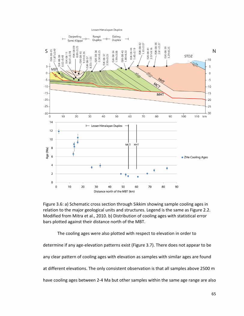
Figure 3.6: a) Schematic cross section through Sikkim showing sample cooling ages in relation to the major geological units and structures. Legend is the same as Figure 2.2. Modified from Mitra et al., 2010. b) Distribution of cooling ages with statistical error bars plotted against their distance north of the MBT.
The cooling ages were also plotted with respect to elevation in order to
determine if any age-elevation patterns exist (Figure 3.7). There does not appear to be
any clear pattern of cooling ages with elevation as samples with similar ages are found
at different elevations. The only consistent observation is that all samples above 2500 m
have cooling ages between 2-4 Ma but other samples within the same age range are also
65
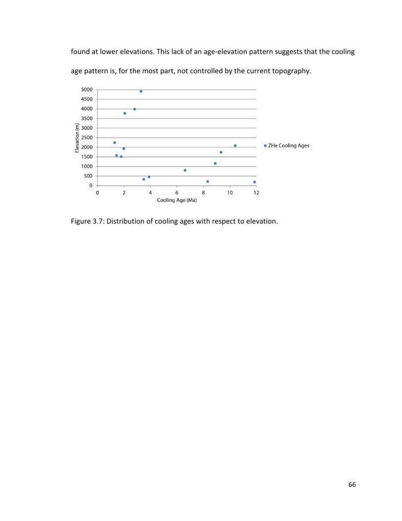
found at lower elevations. This lack of an age-elevation pattern suggests that the cooling
age pattern is, for the most part, not controlled by the current topography.
Figure 3.7: Distribution of cooling ages with respect to elevation.
66

Chapter 4 - Interpretation of ZHe Ages and Numerical Modelling Results
This section introduces the thermal model used in this study and provides
justification for the use of thermo-kinematic modelling for interpreting
thermochronological data in continental areas where the thermal state of the crust is
perturbed by active tectonics.
4.1 - Thermal Field in the Continental Crust
A cooling age depends both on the spatial and temporal evolution of the thermal
field and on the rock particle pathway as material travels through the crust during
exhumation. Consequently, the way heat is produced, diffused and advected within the
crust is integral to the interpretation of thermochronological data. The following section
briefly outlines the characteristics of the crustal thermal field and how it is perturbed by
geological processes.
It has long been recognised that the temperature beneath the surface increases
with depth with typical values of the geothermal gradient, the rate at which the
subsurface temperature changes with depth, of 20-30 °C/km measured in mines and
deep drill holes (Beardsmore and Cull, 2001). Within the upper crust, the geothermal
gradient depends on the heat flux into the base of the crust, the heat production within
the crust, the thermal properties of the rocks, and the effects of topography, faulting,
erosion and sedimentation, which affect the spacing and shape of isotherms (e.g.,
Mancktelow and Grasemann, 1997; Ehlers, 2005). In one dimension, the heat flux within
the earth can be calculated using Fourier’s Law (e.g., Beardsmore and Cull, 2001):
𝑞 = −𝑘 𝑑𝑇𝑑𝑧
(Eq. 4.1)
67
where q is the heat flow, k is the thermal conductivity and dT/dz is the geothermal
gradient. There is significant variability in surface heat flow at both regional and global
scale (Ehlers, 2005). The thermal conductivity of rocks near the surface generally ranges
between 2-3 W/m*k (Beardsmore and Cull, 2001) measured through laboratory tests.
Thermal conductivity measurements of GHS gneisses from Nepal show a range of 2-3
W/m*k perpendicular to the foliation and a much greater range of 2.4-5 W/m*k parallel
to the foliation (Whipp et al., 2007).
Within the earth, significant quantities of crustal heat are produced in situ
through radioactive decay of 238U, 235U, 232Th and 40K (e.g., Urey et al., 1955), accounting
for up to 80% of the heat flux emanating from the crust at the surface today
(Beardsmore and Cull, 2001). The value of heat production varies both horizontally and
vertically due to changing rock types (Ehlers, 2005) and concentrations of heat-
producing elements, and hence contributes to spatial variation in the geothermal
gradient. Data from the GHS in Nepal suggests an average range of radiogenic heat
production of ~1-3 µW/m3 (England et al., 1992; Whipp et al., 2007).
4.1.1 - The Effects of Thrust Faulting on the Crustal Thermal Field
Within the crust, heat is transferred by two processes: conduction and advection
(Beardsmore and Cull, 2001). Conductive heat transfer in the presence of a temperature
gradient results from molecular interactions without any net movement of rock.
Advection, on the other hand, involves the movement of heat by physical displacement
of rock, magma or fluid. In large convergent orogens, thrust faults transport not only
crustal material but also the heat associated with that material (Ehlers and Farley, 2003
68
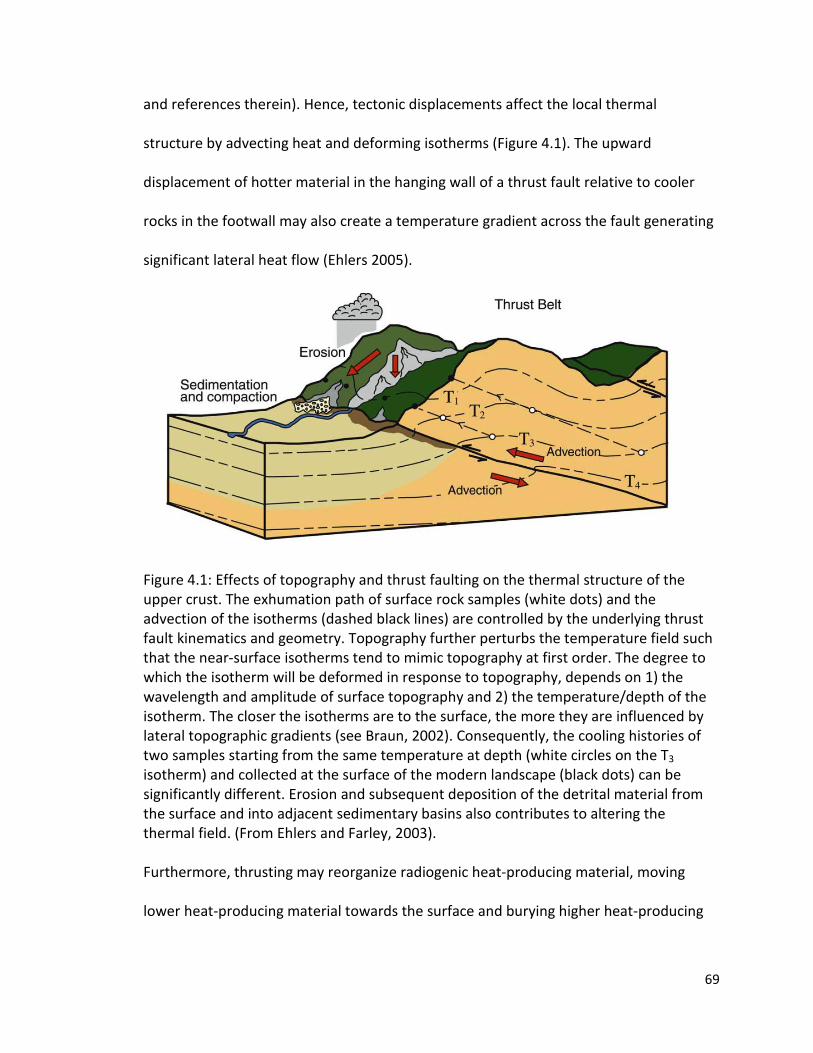
and references therein). Hence, tectonic displacements affect the local thermal
structure by advecting heat and deforming isotherms (Figure 4.1). The upward
displacement of hotter material in the hanging wall of a thrust fault relative to cooler
rocks in the footwall may also create a temperature gradient across the fault generating
significant lateral heat flow (Ehlers 2005).
Figure 4.1: Effects of topography and thrust faulting on the thermal structure of the upper crust. The exhumation path of surface rock samples (white dots) and the advection of the isotherms (dashed black lines) are controlled by the underlying thrust fault kinematics and geometry. Topography further perturbs the temperature field such that the near-surface isotherms tend to mimic topography at first order. The degree to which the isotherm will be deformed in response to topography, depends on 1) the wavelength and amplitude of surface topography and 2) the temperature/depth of the isotherm. The closer the isotherms are to the surface, the more they are influenced by lateral topographic gradients (see Braun, 2002). Consequently, the cooling histories of two samples starting from the same temperature at depth (white circles on the T3 isotherm) and collected at the surface of the modern landscape (black dots) can be significantly different. Erosion and subsequent deposition of the detrital material from the surface and into adjacent sedimentary basins also contributes to altering the thermal field. (From Ehlers and Farley, 2003). Furthermore, thrusting may reorganize radiogenic heat-producing material, moving
lower heat-producing material towards the surface and burying higher heat-producing
69
material originally located near the surface, adding to the effects of heat advection and
further perturbing the subsurface thermal field (Ehlers, 2005).
4.1.2 - Topographic Effects on the Thermal Structure
Analytical solutions and numerical models from Mancktelow and Grasemann
(1997) show that the amplitude and wavelength of topography are also important
parameters controlling the subsurface thermal structure. The temperature at the
surface represents a thermal boundary for the rocks in the subsurface so that the
temperature of the rocks just below the surface is effectively the same as that of the air
above the surface. This thermal boundary forces the subsurface thermal field to deform
in response to changes in topography at the surface. In tectonically active areas the
near-surface isotherms roughly mimic the shape of the overlying topography. The
wavelength of the topography and the local exhumation rate are the major controls on
the depth of penetration of the topographic disturbance; the disturbance decays
exponentially with depth proportionally with the wavelength of the topography
(Beardsmore and Cull, 2001; Braun, 2002). Because of this, thermochronometric systems
with lower closure temperatures (e.g., AHe) are more influenced by topography than
systems with higher closure temperatures (e.g., ZHe or muscovite Ar/Ar) (Figure 4.2).
As represented in Figures 4.1 and 4.2, topography in areas of high relief can
dramatically perturb sub-surface isotherms by decreasing the geothermal gradient
beneath topographic highs, and increasing it under the valleys. Assuming a vertical
particle trajectory, the thermochronological ages in these locations will be older and
younger, respectively, than if topography were flat (Ehlers and Farley, 2003). Braun
70

(2005; and references therein) showed that the thermal effects of topography can lead
to a larger uncertainty on thermochronological ages than the analytical error of age
determination itself, suggesting a significant thermal influence that can be detected in
thermochronological data.
Figure 4.2: Modelled effects of surface topography in three-dimensions on the apatite helium (60°C) and apatite fission track (110° C) closure isotherms at Mt. Waddington, BC, Canada. The upper layer represents surface topography. The two underlying layers represent the subsurface topography of the 60°C and 110°C isotherms, respectively. Mountain ridges and river valleys at the surface are mimicked to some degree by the underlying thermal structure due to the conduction of heat. Deeper isotherms are less perturbed than shallower ones. This thermal model ran for 15 Ma under steady-state topography with a uniform exhumation rate of 0.5 mm/yr. (From Ehlers and Farley, 2003).
4.1.3 - Erosion and Sedimentation
Erosion and sedimentation also have a large effect on the crustal thermal
structure, which is combined with the effects of topography and faulting in nature
(Figure 4.3 & 4.4). Erosion results in the upward advection of relatively warm rock
71

toward the surface, thereby increasing the geothermal gradient and producing relatively
younger cooling ages. At low rates of erosion (<1 km/Ma) the rate of change of affected
cooling ages is nearly 1:1 (on a log-log scale) with the rate of erosion, and the majority of
heat is transferred by conduction (Reiners and Brandon, 2006; Figure 4.3). At higher
rates of erosion, material is removed fast enough for advection of heat to play a major
role. In this case, as the rate of erosion increases, affected cooling ages decrease at a
much higher rate (Reiners and Brandon, 2006; Figure 4.3).
Figure 4.3: Effects of erosion rate on cooling ages of different thermochronometers from low temperature (apatite helium) to high temperature (hornblende argon). Scale is in log-log format. Cooling ages were calculated for each thermochronometer using a 1-D thermal model with a steady erosion rate. From Reiners and Brandon 2006.
72
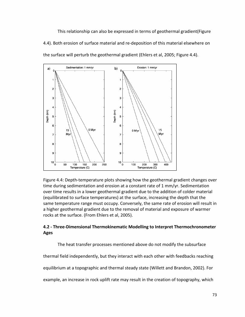
This relationship can also be expressed in terms of geothermal gradient(Figure
4.4). Both erosion of surface material and re-deposition of this material elsewhere on
the surface will perturb the geothermal gradient (Ehlers et al, 2005; Figure 4.4).
Figure 4.4: Depth-temperature plots showing how the geothermal gradient changes over time during sedimentation and erosion at a constant rate of 1 mm/yr. Sedimentation over time results in a lower geothermal gradient due to the addition of colder material (equilibrated to surface temperatures) at the surface, increasing the depth that the same temperature range must occupy. Conversely, the same rate of erosion will result in a higher geothermal gradient due to the removal of material and exposure of warmer rocks at the surface. (From Ehlers et al, 2005). 4.2 - Three-Dimensional Thermokinematic Modelling to Interpret Thermochronometer Ages
The heat transfer processes mentioned above do not modify the subsurface
thermal field independently, but they interact with each other with feedbacks reaching
equilibrium at a topographic and thermal steady state (Willett and Brandon, 2002). For
example, an increase in rock uplift rate may result in the creation of topography, which
73

in turn enhances localized erosion, which may help sustain local rock uplift, all of which
will modify the thermal field. The complex interactions between heat transfer processes
modify the sub-surface thermal field in active convergent orogens and cannot be
accounted for using simple analytical solutions and/or 1D thermal models. Instead, low-
temperature thermochronometer data from these regions should be interpreted using
3D thermal and age prediction models, capable of predicting the evolution of the
thermal field and taking into account complex (i.e., non-vertical) rock exhumation paths.
The set of cooling ages presented in Chapter 3 contains a record of crustal
cooling that is sensitive to the major tectonic structures controlling exhumation of the
samples. However, the cooling history recorded in rock samples results from a
combination of kinematic and thermal effects and is therefore non-unique. To address
the issue of non-unique mineral cooling histories, I use a modified version of the
thermokinematic model Pecube (Braun, 2003; Braun et al., 2012) in combination with a
formal inversion software package (Neighbourhood Algorithm; Sambridge 1999a & b)
that can define the range of model parameters that is consistent with the observed
cooling age data. The inversion involves two steps: sampling of the input parameter
ranges for multiple variables to identify combinations that provide a good fit to the
observed cooling age data; and then appraising the search results to place statistical
bounds on the parameter values that provide a good fit.
4.2.1 - The Pecube Software
The Pecube software (Braun, 2003; Braun et al., 2012) calculates the 3D thermal
field and predicted mineral cooling age distributions over a set period of geologic time in
74
a model domain using input thermal and material parameters, topography and fault
kinematic data. The predicted cooling ages, and age distributions, can then be compared
to the observed cooling ages in order to determine a misfit to the data, and model
parameters can be varied over defined parameter ranges in order to minimize the
goodness-of-fit. Pecube and similar software packages have been used to study
exhumation in the Himalaya in several previous studies (e.g., Whipp et al., 2007; Herman
et al., 2010; Robert et al., 2011; Adlakha et al., 2013; Coutand et al., 2014).
Pecube consists of three major model components: 1) a kinematic model that
calculates rock exhumation paths in three dimensions based on the specified slip rate
and geometry of faults, 2) a thermal model that calculates the crustal thermal field
based on input thermal parameters of the crust, fault motion, surface topography,
surface erosion and/or sedimentation and thermal boundary conditions at the base,
sides and surface of the model, and 3) an age prediction model that predicts various
thermochronologic ages from thermal histories defined by the first two components.
Kinematic Component
Rock transport in Pecube is controlled by user-defined fault geometries and the
convergence rate accommodated by the faults. The convergence rate is partitioned into
overthrusting and underthrusting by a user-defined ratio of underthrusting to total
convergence. Braun et al. (2012) included thermal advection in three dimensions in
order to model the effects of faulting on thermochronological data sets and the thermal
field properly. Faults in Pecube must be defined in a local coordinate system (r,s)
different than the one used to define the model space itself (x, y, z). Each vertex
75
constructing the fault is defined by a pair of coordinates (r, s) where r represents the
horizontal distance and s the vertical depth from the surface trace of the fault (Braun,
2003). The movement histories of the faults, in the case of our models a large thrust
fault, are input into the model. Slip velocities along faults are controlled by a
combination of the convergence between both sides of the model (i.e.,, the Indo-
Tibetan convergence rate) and a partitioning factor that defines overthrusting and
underthrusting slip velocities as the ratio of the rate of underthrusting of the footwall to
the total convergence rate; the reciprocal of this ratio provides the ratio of
overthrusting. Lateral advection of the model topography (Whipp et al., 2009; Coutand
et al., 2014) is also included to ensure rock samples above a thrust fault move nearly
vertically upward during exhumation. This is important because rock transport above
shallow décollement faults can produce nonsensical rock exhumation pathways (where
particles exit and then re-enter the ground) when topography is assumed to be in steady
state (see Appendix F of Coutand et al., 2014).
Thermal Component
The thermal model uses the finite element method to solve the heat transport
equation within a crustal block taking into account uplift and surface erosion of the
block. The transient 3D heat-transport equation solves for temperature iteratively in
three dimensions over time (Braun, 2003; Braun et al., 2012):
𝑑𝑇𝑑𝑡
+ 𝑢 𝑑𝑇𝑑𝑥
+ 𝑣 𝑑𝑇𝑑𝑦
+ 𝑤 𝑑𝑇𝑑𝑧
= 𝑑𝑑𝑥𝑘 𝑑𝑇𝜕𝑥
+ 𝑑𝑑𝑦𝑘 𝑑𝑇𝑑𝑦
+ 𝑑𝑑𝑧𝑘 𝑑𝑇𝑑𝑧
+ 𝐴 (Eq. 4.2)
where T is temperature , t is time, x, y and z are the spatial coordinates, u, v and w are
the advection velocity components, k is the thermal conductivity of the rocks and A is
76
the radiogenic heat production. An initial thermal field is calculated through a
combination of the velocity field controlled by fault motion, input thermal parameters
and thermal boundary conditions such as the temperature at the base of the model and
at the surface. The model has a constant surface and basal temperature and the sides of
the model require no heat flux. An option to consider the thermal influence of
groundwater flow is not included in the current version of Pecube so it was not
considered in these models as modifying the code to include this was beyond the scope
of this study.
Age Prediction Component
Prediction of cooling ages relies on the user-defined fault-slip and temperature
parameters used to construct the thermal and kinematic models. To do this,
thermochronological samples are first positioned on the surface of the model at their
sample locations and then the modelled velocity field is used in reverse to return the
samples to their initial model locations at depth. From their starting positions at depth,
particle thermal histories are generated as particles are transported to the surface using
the prescribed kinematic model. The resulting thermal histories are then used for age
prediction. The age-prediction model for the zircon (U-Th)/He system uses the numerical
scheme of Wolf et al. (1998) and the kinetic parameters of Reiners et al. (2004), based
on a 100 µm grain size (Braun et al., 2012). Cooling ages are predicted from the time-
temperature paths recorded for surface sample locations at each time step specified
(Braun et al., 2012).
77
4.2.2 - Forward Modelling
In order to model cooling ages, Pecube requires a certain number of input
thermal/physical parameters, such as thermal diffusivity, radiogenic heat production,
rock density and heat capacity. In addition, surface and basal temperatures, fault
movement velocity, model simulation time, and topography must be defined.
Topography can also be included using a DEM (digital elevation model). Model output
includes,the 3-dimensional thermal distribution over the model domain at specific time
steps, as well as the predicted cooling ages of rock particles that reach the surface of the
model.
4.3 - Neighbourhood Algorithm (NA) Inversion
Combining Pecube with the Neighbourhood Algorithm (NA) (Sambridge, 1999a &
b; Rickwood and Sambridge, 2006) provides the ability to perform inverse modelling of
cooling age data sets (Braun et al., 2012). These inverse models are used to define the
range of input parameters that produce predicted cooling ages consistent with the
observed ages. Rather than testing model parameters randomly, the NA attempts to
determine the parameter ranges that fit the observed ages in a guided search of the
regions of the parameter space that provide a low misfit to the data. The misfit function
calculated in Pecube (Braun et al., 2012) is:
𝜑 = 1𝑛 �∑
(𝑃𝑟𝑒𝑑𝐴𝑔𝑒𝑖−𝑂𝑏𝑠𝐴𝑔𝑒𝑖)2
𝜎𝑖2
𝑛𝑖=1 (Eq.4.3)
where n is the number of thermochronologic ages, σ is the 1-sigma uncertainty
associated with the measured thermochronometer ages, PredAge is the predicted age
and ObsAge is the observed age. First, the NA sampling stage assesses input
78

thermochronological data in order to constrain optimal values and combinations of the
free parameters; second, the NA appraisal stage calculates the probability of these
parameter values taking into account the uncertainty associated with the cooling ages
and the sensitivity of the model parameters to these uncertainties. Braun et al. (2012)
found that ~10000 models is generally enough to invert for 5-6 free parameters to
converge on lowest misfit values, but this number increases with additional free
parameters.
In order to guide the inversion to areas within the parameter space that have the
lowest misfit values in the search stage, the parameter space is divided into a set of
Voronoï cells (Sambridge, 1999). Each of these cells is assigned a calculated misfit value
so that input values for proceeding models within the inversion will be taken from cells
with the lowest misfit, thereby directing the inversion to parameter ranges most likely to
yield a good fit to the data. A resample ratio can be specified that corresponds to the
ratio of Voronoï cells resampled to the total number of cells in the NA iteration (Braun et
al., 2012). The higher this ratio, the longer the inversion will take to converge.
Conversely, a lower resampling ratio will converge more quickly but possibly miss parts
of the parameter space that fit the data well. Satisfactory convergence on lowest misfit
values has been achieved using resampling ratios from 50 to 90% (Braun et al., 2012).
We use a 90% resampling ratio for our inversions, at the expense of longer model run
times, as this reduces the chances of missing local minimum misfit values that may
otherwise be overlooked. A misfit value of < 1 suggests that the modelled cooling ages
fit the data within the analytical error of the samples (Braun et al., 2012).
79
4.4 - Numerical Model Design
The Pecube models extend from just south of the trace of the MBT at 26.5 °N to
~160 km north at 28.0 °N and from 88 to 89 °E, an area that contains nearly all of Sikkim
(Figure 2.1). The base of the model was set at 50 km depth in order to model the MHT.
The DEM used to define the model topography was constructed using data from SRTM-
90 taken from the CGIAR-CSI (http://srtm.csi.cgiar.org/). In the models presented below,
topography is assumed to be in steady state.
The model was set up so that a single basal thrust fault equivalent to the MHT-
MBT/MFT is active during the model run. Available geophysical data were used to place
constraints on the location and geometry of the MHT; the MHT in Sikkim is interpreted
to have a ramp-and-flat morphology rather than descending at a constant angle into the
subsurface (e.g., INDEPTH; Acton et al., 2011). This fault slips at a constant rate over a
specified time interval (12 Ma) in order to model the movement along the MHT from the
mid-Miocene to present. All models run from 12-0 Ma because this timeframe
encompasses the range of our data. In addition, activity on the major thrust faults north
of the MBT (MCTZ and STDZ) are suggested to have ceased by this time (e.g., Catlos et
al., 2004; Harris et al., 2004) while subsequent India-Eurasia convergence has likely been
accommodated through displacement on the MBT/MFT and structural duplexing within
the LHS. The rate of fault slip is defined by the convergence rate and a partitioning ratio
that defines the proportion of underthrusting of India to overthrusting of Eurasia:
𝜆 = 𝑣𝑢𝑣𝑐𝑜𝑛𝑣
(Eq. 4.4)
80
where λ is the partitioning ratio, νconv is the convergence velocity and νu is the
underthrusting velocity. The partitioning ratio is necessary in the model setup, because
although only a single fault is being modelled, it must be input into Pecube as two
separate faults occupying the same coordinates, one moving to the south representing
motion on the hanging wall block and one moving north representing motion on the
footwall block. Both the footwall and hanging wall blocks move with respect to the fault
itself. The modelled MHT reaches the surface through the trace of the MBT. In Sikkim,
the MBT and MFT are very close to one another (within 15 km), but the MBT was chosen
because its position is more accurately mapped (Figure 2.1). In addition, the MFT is
thought to have been active only after the Miocene (Mukul, 2007) and the MBT is likely
to have been active since 12-10 Ma (Catlos et al., 2004; Harris et al., 2004; Coutand et
al., 2014). A list of model input parameters common to all of the simulations can be
found in Table 4.1. Of the 16 ZHe ages obtained (see Chapter 3), only 15 were used
during modelling. Sample ISIK-08-01 was not used because it is assumed to be un-reset.
This sample was taken from the sedimentary rocks of the Siwaliks to the south of the
MBT. The sample has an average cooling age of 12.94±1.05 Ma, much older than the
suggested quaternary activation of the MFT, which is the basal thrust of the thrust sheet
the sample was taken from. Also, the Siwaliks are the product of syn-orogenic erosion of
material washed down from further north into the foreland basin and any zircons
present would be considered detrital. This suggests that the cooling age is likely
recording a previous thermal event and that the sample did not cool from its closure
temperature to the surface within the MFT thrust sheet.
81
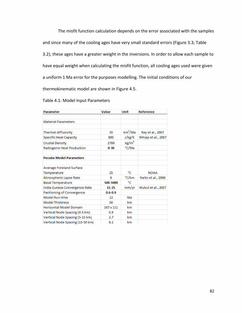
The misfit function calculation depends on the error associated with the samples
and since many of the cooling ages have very small standard errors (Figure 3.3; Table
3.2), these ages have a greater weight in the inversions. In order to allow each sample to
have equal weight when calculating the misfit function, all cooling ages used were given
a uniform 1 Ma error for the purposes modelling. The initial conditions of our
thermokinematic model are shown in Figure 4.5.
Table 4.1: Model Input Parameters
82
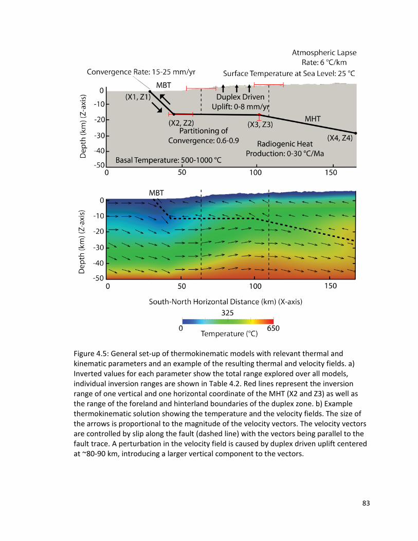
Figure 4.5: General set-up of thermokinematic models with relevant thermal and kinematic parameters and an example of the resulting thermal and velocity fields. a) Inverted values for each parameter show the total range explored over all models, individual inversion ranges are shown in Table 4.2. Red lines represent the inversion range of one vertical and one horizontal coordinate of the MHT (X2 and Z3) as well as the range of the foreland and hinterland boundaries of the duplex zone. b) Example thermokinematic solution showing the temperature and the velocity fields. The size of the arrows is proportional to the magnitude of the velocity vectors. The velocity vectors are controlled by slip along the fault (dashed line) with the vectors being parallel to the fault trace. A perturbation in the velocity field is caused by duplex driven uplift centered at ~80-90 km, introducing a larger vertical component to the vectors.
83
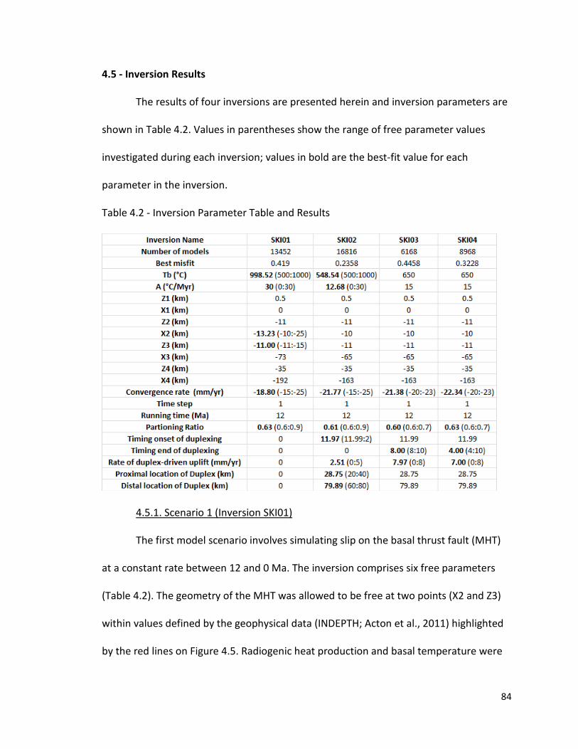
4.5 - Inversion Results
The results of four inversions are presented herein and inversion parameters are
shown in Table 4.2. Values in parentheses show the range of free parameter values
investigated during each inversion; values in bold are the best-fit value for each
parameter in the inversion.
Table 4.2 - Inversion Parameter Table and Results
4.5.1. Scenario 1 (Inversion SKI01)
The first model scenario involves simulating slip on the basal thrust fault (MHT)
at a constant rate between 12 and 0 Ma. The inversion comprises six free parameters
(Table 4.2). The geometry of the MHT was allowed to be free at two points (X2 and Z3)
within values defined by the geophysical data (INDEPTH; Acton et al., 2011) highlighted
by the red lines on Figure 4.5. Radiogenic heat production and basal temperature were
84
left free between 0-30 °C/Ma and 500-1000 °C, respectively. The total Indo-Tibetan
convergence rate was allowed to vary between 15-25 mm/yr which is within the
estimates of 15-20 mm/yr in Sikkim (Mukul et al., 2010) and 21±1.5 mm/yr in Nepal
(Lavé and Avouac, 2000). The partitioning rate was given a large range of 0.6-0.9,
consistent with other kinematic modelling studies elsewhere in the Himalaya (Whipp et
al., 2007; Herman et al., 2010; Robert et al., 2011; Coutand et al., 2014). The complete
set of parameters used for this model is shown in Table 4.2.
SKI01 Inversion Results
A total of 13452 forward models were run using the NA module and the results
are shown in Table 4.2 and Figure 4.6. The lowest misfit model produced a misfit of
0.419, which indicates an overall good fit to the dataset. In this inversion, the lowest
misfit values for the thermal parameters are at the high end of the input ranges of the
inputs, with a preferred basal temperature of ~1000 °C and a heat production of ~30
°C/Ma (Figure 4.6a). These thermal values produce an unrealistically high geothermal
gradient which would result in the melting of most rocks near the base of the model
suggesting that the best-fit modelled thermal field for this scenario is improbable. The
best-fit convergence rate is near the lower end of the range given with a rate of 18.8
mm/yr as is the partitioning factor at 0.63 which suggests ~40% of the total convergence
(~7 mm/yr) is accommodated through overthrusting (Figure 4.5b). These values reflect
an attempt by the model to generate and match young ages observed in parts of the
hanging wall by producing higher temperatures and a higher proportion of overthrusting
which all result in more upward advection of heat, faster cooling, and younger ages. The
85
fault point Z3 yielded a lowest misfit value of 11 km, which results in a flat section of the
MHT between two ramps; point X2 returned a value of ~13.2 km north of the MBT
(Figure 4.6c). The resulting fault geometry matches the available geophysical data very
well, resulting in a steep frontal ramp dipping at ~39° followed by a consistently flat
section and finally a deeper but shallower angle ramp dipping at ~11°. The 1 and 2-D
PDFs, illustrate how certain parameters are not well defined despite the low misfit value
obtained for the best forward model. For example, the radiogenic heat production and
partitioning ratio show normal distributions in the 1D Probability Density Functions
(PDFs) (Figures 4.6a & b), while 2D PDFs show that basal temperature and convergence
rates are poorly defined within 1σ error (Figures 4.6 a & b).
SKI01 Forward Model
Using the free parameter values determined by the lowest misfit model from the
inversion, a single forward model was run at high resolution to compare the predicted
and observed cooling ages (Figure 4.7).
The predicted ages fit the general pattern of the observed ages but quite a few
samples show more than a 1 Ma difference. The six most southern ages do not match
well, especially the oldest age north of the MBT where the predicted age is more than 3
Ma too young. North of the HHT the predicted ages change from being older than the
observed ages to being younger towards the north, although the ages all match within
error. In the central part of the section predicted ages are consistently older than the
observed ages (Figure 4.7). The velocity field that controls this age pattern is shown in
Figure 4.8.
86
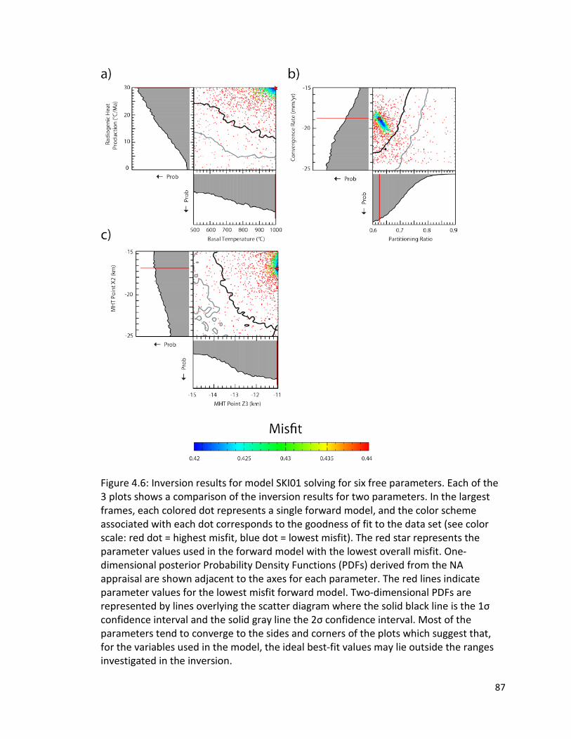
Figure 4.6: Inversion results for model SKI01 solving for six free parameters. Each of the 3 plots shows a comparison of the inversion results for two parameters. In the largest frames, each colored dot represents a single forward model, and the color scheme associated with each dot corresponds to the goodness of fit to the data set (see color scale: red dot = highest misfit, blue dot = lowest misfit). The red star represents the parameter values used in the forward model with the lowest overall misfit. One-dimensional posterior Probability Density Functions (PDFs) derived from the NA appraisal are shown adjacent to the axes for each parameter. The red lines indicate parameter values for the lowest misfit forward model. Two-dimensional PDFs are represented by lines overlying the scatter diagram where the solid black line is the 1σ confidence interval and the solid gray line the 2σ confidence interval. Most of the parameters tend to converge to the sides and corners of the plots which suggest that, for the variables used in the model, the ideal best-fit values may lie outside the ranges investigated in the inversion.
87
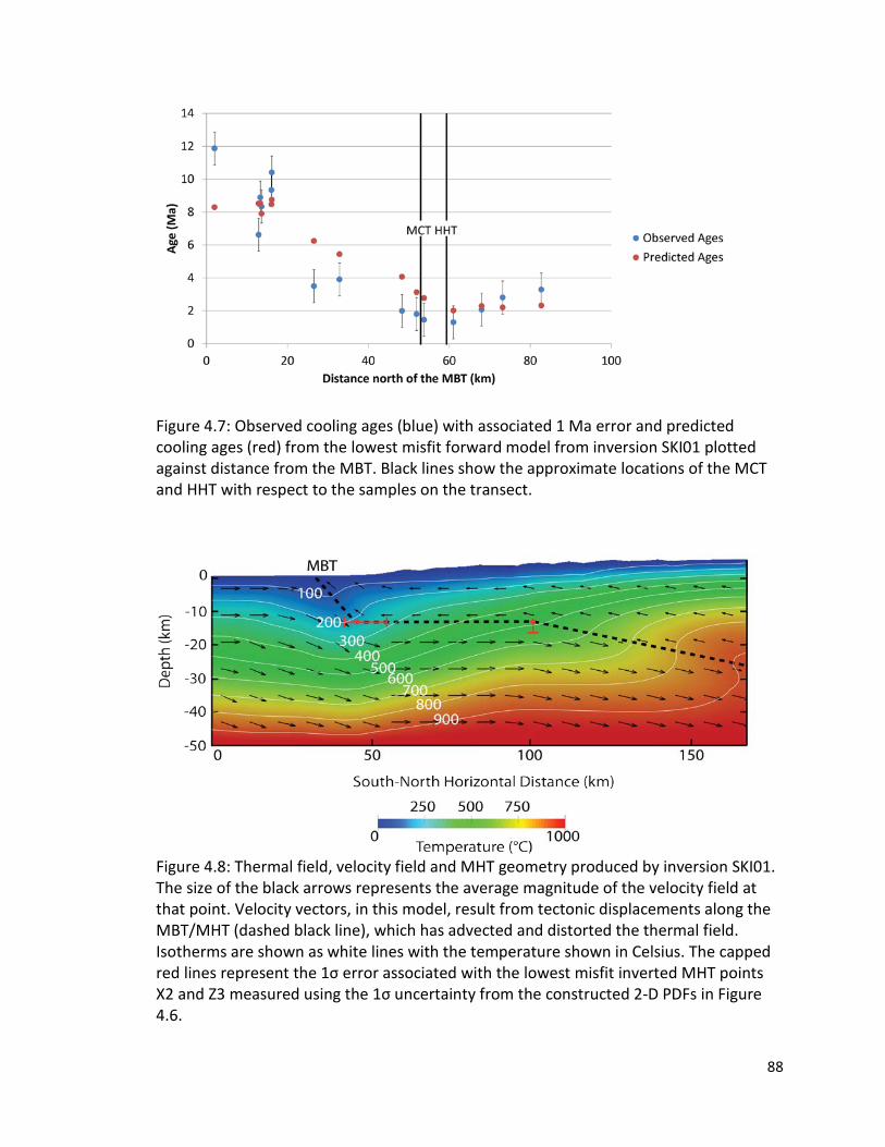
Figure 4.7: Observed cooling ages (blue) with associated 1 Ma error and predicted cooling ages (red) from the lowest misfit forward model from inversion SKI01 plotted against distance from the MBT. Black lines show the approximate locations of the MCT and HHT with respect to the samples on the transect.
Figure 4.8: Thermal field, velocity field and MHT geometry produced by inversion SKI01. The size of the black arrows represents the average magnitude of the velocity field at that point. Velocity vectors, in this model, result from tectonic displacements along the MBT/MHT (dashed black line), which has advected and distorted the thermal field. Isotherms are shown as white lines with the temperature shown in Celsius. The capped red lines represent the 1σ error associated with the lowest misfit inverted MHT points X2 and Z3 measured using the 1σ uncertainty from the constructed 2-D PDFs in Figure 4.6.
88
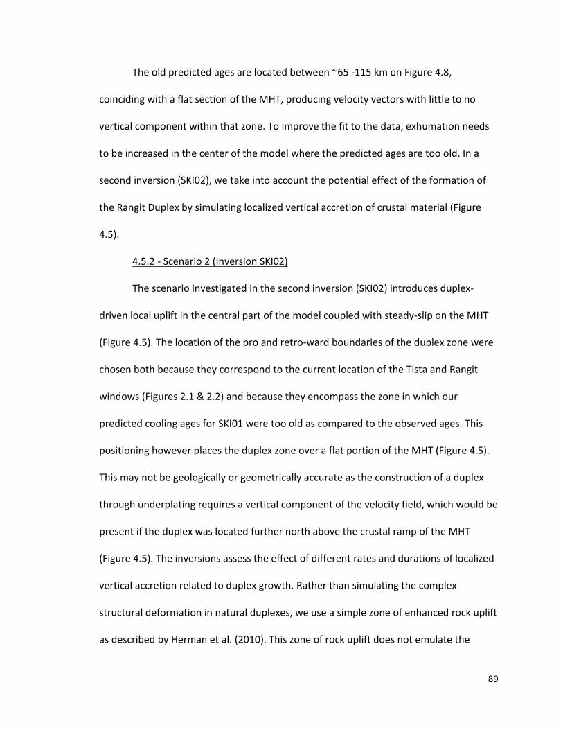
The old predicted ages are located between ~65 -115 km on Figure 4.8,
coinciding with a flat section of the MHT, producing velocity vectors with little to no
vertical component within that zone. To improve the fit to the data, exhumation needs
to be increased in the center of the model where the predicted ages are too old. In a
second inversion (SKI02), we take into account the potential effect of the formation of
the Rangit Duplex by simulating localized vertical accretion of crustal material (Figure
4.5).
4.5.2 - Scenario 2 (Inversion SKI02)
The scenario investigated in the second inversion (SKI02) introduces duplex-
driven local uplift in the central part of the model coupled with steady-slip on the MHT
(Figure 4.5). The location of the pro and retro-ward boundaries of the duplex zone were
chosen both because they correspond to the current location of the Tista and Rangit
windows (Figures 2.1 & 2.2) and because they encompass the zone in which our
predicted cooling ages for SKI01 were too old as compared to the observed ages. This
positioning however places the duplex zone over a flat portion of the MHT (Figure 4.5).
This may not be geologically or geometrically accurate as the construction of a duplex
through underplating requires a vertical component of the velocity field, which would be
present if the duplex was located further north above the crustal ramp of the MHT
(Figure 4.5). The inversions assess the effect of different rates and durations of localized
vertical accretion related to duplex growth. Rather than simulating the complex
structural deformation in natural duplexes, we use a simple zone of enhanced rock uplift
as described by Herman et al. (2010). This zone of rock uplift does not emulate the
89
stacking of imbricates as a real duplex would so internal shortening that would occur
within the duplex zone is not accounted for.
In this inversion, the basal temperature, radiogenic heat production,
convergence rate and partitioning were given the same range as the previous SKI01
inversion but additional parameters were added to allow for an area of localized uplift
representing the growth of a duplex in the model space above the MHT (Table 4.2).
There is virtually no published geological information regarding the timing of activity,
rate or spatial extent of duplexing in Sikkim. The timing of duplex initiation was allowed
to vary between ~12 Ma and 2 Ma while the end time was fixed to 0 Ma. The rate of
vertical uplift attributed to duplexing varied between 0 - 5 mm/yr. Since both the timing
and the rate of duplexing is poorly resolved, both were given large ranges in order for
Pecube to properly access the parameter space. Finally, the southern boundary of the
duplex was given a range of 20 - 40 km north of the MBT and the northern boundary
was given a range of 60 - 80 km north of the MBT (Figure 4.5).
SKI02 Inversion Results
A total of 16816 models were run during this inversion (Table 4.2, Figure 4.9)
with a lowest misfit value of 0.236, which is considerably lower than the lowest misfit
obtained in the previous inversion SKI01. The thermal parameters yielded more
reasonable values during this run with a basal temperature of 549 °C and a radiogenic
heat production of 12.68 °C/Ma (Figure 4.9a). These values are well within the
parameter range specified, which suggests that they likely represent geologically more
realistic values for this tectonic scenario. The convergence rate and partitioning ratio
90

yielded values of 21.77 mm/yr and 0.61, respectively (Figure 4.9b). These results still
favour rapid uplift and exhumation of the hanging wall of the MHT. The preferred duplex
initiation time (11.97 Ma) is essentially identical to the time at which the model starts,
so that the duplex is active during the entire model run at an uplift rate of 2.51 mm/yr,
in the middle of the defined range (Figure 4.9c). Finally the lowest misfit values for
boundaries of the duplex are 28.75 km and 79.89 km (north of the MBT) for the
southern and northern boundaries, respectively (Figure 4.9d).
As in SKI01 the 1 and 2-D PDFs suggest that many of the parameters are not well
defined within the data ranges input in the model. The partitioning ratio once again
shows the closest to a normal distribution while the heat production, convergence rate,
duplex initiation time and southern duplex boundary parameters show much less
distinct increases in probability near the lowest misfit value. The remaining parameters
show very poor distributions with some showing nearly flat distributions and others
showing only very poorly defined peaks.
91
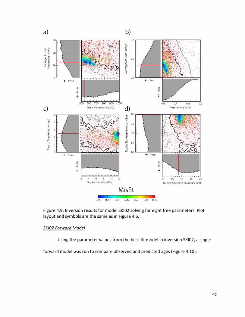
Figure 4.9: Inversion results for model SKI02 solving for eight free parameters. Plot layout and symbols are the same as in Figure 4.6. SKI02 Forward Model
Using the parameter values from the best-fit model in inversion SKI02, a single
forward model was run to compare observed and predicted ages (Figure 4.10).
92
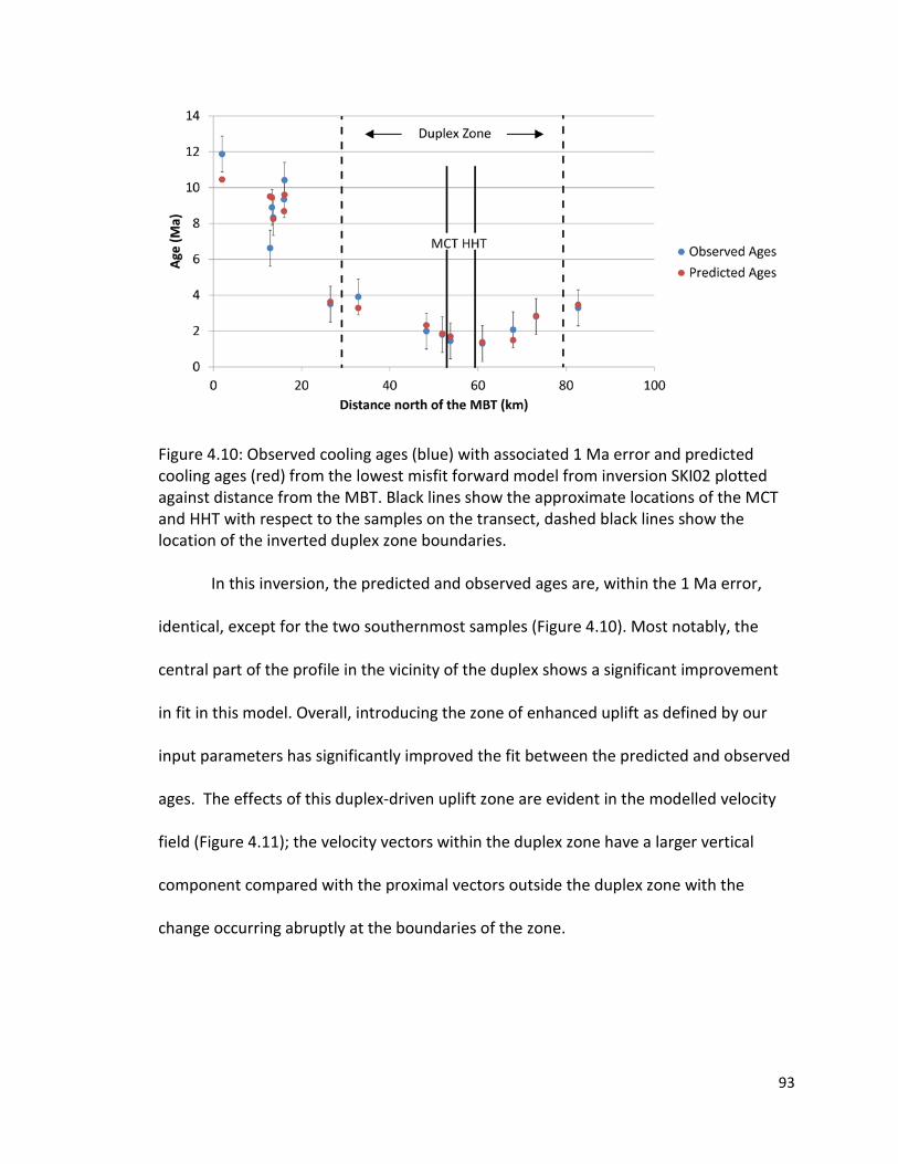
Figure 4.10: Observed cooling ages (blue) with associated 1 Ma error and predicted cooling ages (red) from the lowest misfit forward model from inversion SKI02 plotted against distance from the MBT. Black lines show the approximate locations of the MCT and HHT with respect to the samples on the transect, dashed black lines show the location of the inverted duplex zone boundaries.
In this inversion, the predicted and observed ages are, within the 1 Ma error,
identical, except for the two southernmost samples (Figure 4.10). Most notably, the
central part of the profile in the vicinity of the duplex shows a significant improvement
in fit in this model. Overall, introducing the zone of enhanced uplift as defined by our
input parameters has significantly improved the fit between the predicted and observed
ages. The effects of this duplex-driven uplift zone are evident in the modelled velocity
field (Figure 4.11); the velocity vectors within the duplex zone have a larger vertical
component compared with the proximal vectors outside the duplex zone with the
change occurring abruptly at the boundaries of the zone.
93
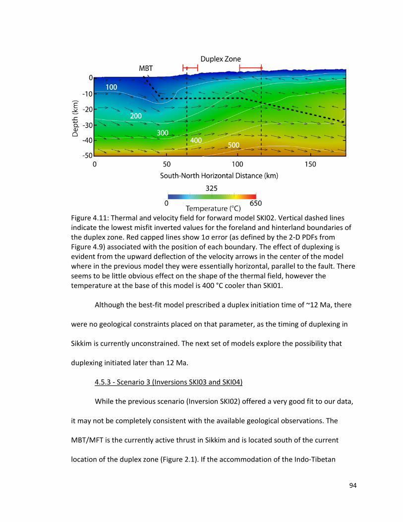
Figure 4.11: Thermal and velocity field for forward model SKI02. Vertical dashed lines indicate the lowest misfit inverted values for the foreland and hinterland boundaries of the duplex zone. Red capped lines show 1σ error (as defined by the 2-D PDFs from Figure 4.9) associated with the position of each boundary. The effect of duplexing is evident from the upward deflection of the velocity arrows in the center of the model where in the previous model they were essentially horizontal, parallel to the fault. There seems to be little obvious effect on the shape of the thermal field, however the temperature at the base of this model is 400 °C cooler than SKI01.
Although the best-fit model prescribed a duplex initiation time of ~12 Ma, there
were no geological constraints placed on that parameter, as the timing of duplexing in
Sikkim is currently unconstrained. The next set of models explore the possibility that
duplexing initiated later than 12 Ma.
4.5.3 - Scenario 3 (Inversions SKI03 and SKI04)
While the previous scenario (Inversion SKI02) offered a very good fit to our data,
it may not be completely consistent with the available geological observations. The
MBT/MFT is the currently active thrust in Sikkim and is located south of the current
location of the duplex zone (Figure 2.1). If the accommodation of the Indo-Tibetan
94

convergence by thrust faulting progressed in sequence from north to south (from the
MCT to the MBT/MFT), then the duplex, which is located between the MCT and MBT,
must have ceased accommodating this shortening, or at least slowed down
considerably, at approximately the time at which the MBT became active or relatively
soon after. This suggests that allowing the duplex to be active during the entire 12 Ma
model run may not be geologically reasonable.
To test the effects of a shorter period of duplex-driven uplift, two inversions
(SKI03 and SKI04) were run with only four free parameters (Table 4.2). Duplexing was set
to start in the model at 12 Ma and to end between 10-8 Ma in SKI03 and 10-4 Ma in
SKI04. The duplexing rate range was increased to 0-8 mm/yr for both inversions to allow
a similar magnitude of rock uplift to Inversion SKI02 within the shorter duration of uplift.
The convergence rate and partitioning ratio were treated as free parameters to allow
the model a larger parameter space to invert for the duplexing parameters. They were
given ranges of 20-23 mm/yr and 0.6-0.7, respectively. Thermal parameters and the
location of the duplex zone were set using best-fit model values obtained from the
previous inversion SKI02.
SKI03 Inversion Results
A total of 6168 models were run for this inversion (Table 4.2, Figure 4.12) with
lowest misfit model yielding a misfit of 0.446, similar to inversion SKI01. The
convergence and partitioning values are approximately the same values as in SKI02, 22.3
mm/yr and 0.63 (Figure 4.12a). The preferred values for the duplex parameters result in
duplex cessation at 8 Ma and a rate of duplex-driven uplift of 8 mm/yr (Figure 4.12b).
95
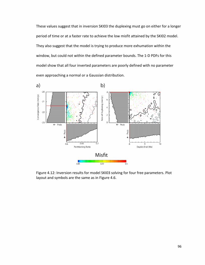
These values suggest that in inversion SKI03 the duplexing must go on either for a longer
period of time or at a faster rate to achieve the low misfit attained by the SKI02 model.
They also suggest that the model is trying to produce more exhumation within the
window, but could not within the defined parameter bounds. The 1-D PDFs for this
model show that all four inverted parameters are poorly defined with no parameter
even approaching a normal or a Gaussian distribution.
Figure 4.12: Inversion results for model SKI03 solving for four free parameters. Plot layout and symbols are the same as in Figure 4.6.
96
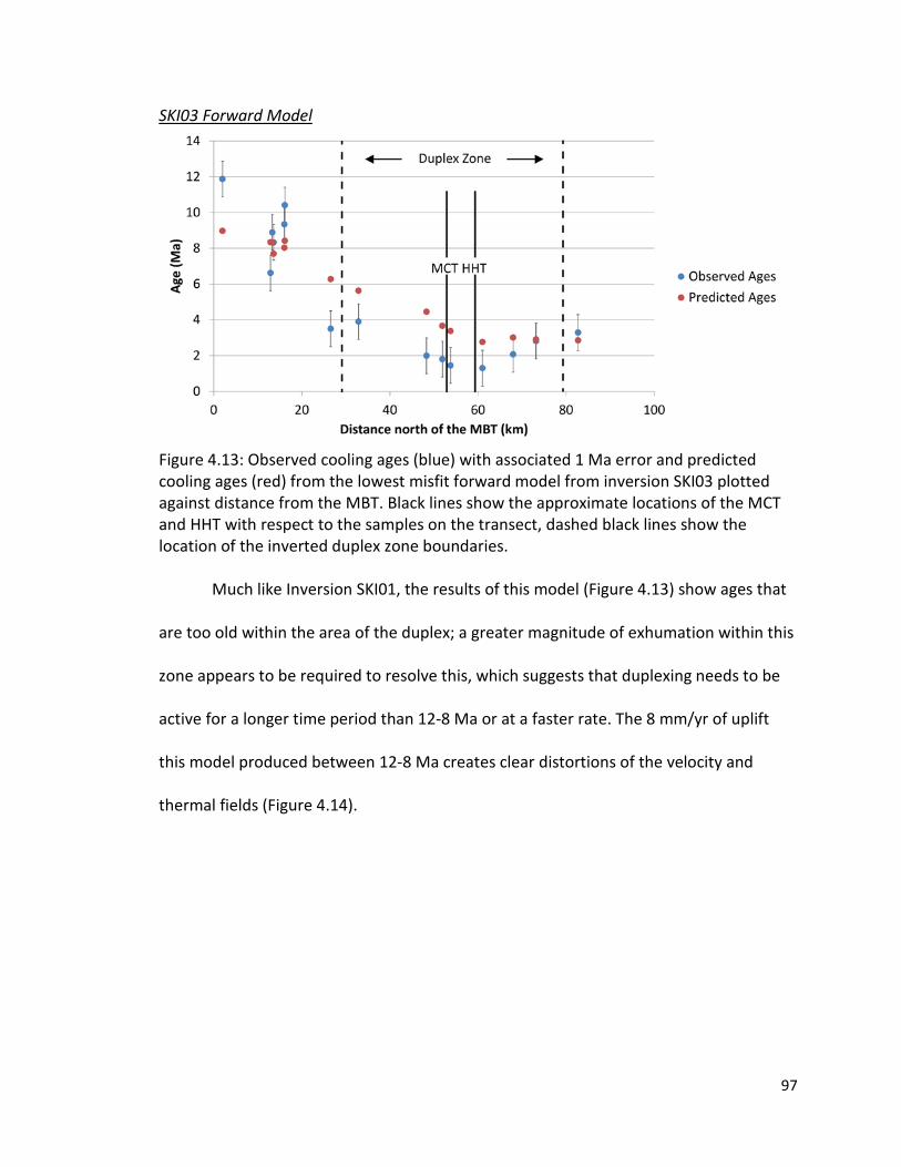
SKI03 Forward Model
Figure 4.13: Observed cooling ages (blue) with associated 1 Ma error and predicted cooling ages (red) from the lowest misfit forward model from inversion SKI03 plotted against distance from the MBT. Black lines show the approximate locations of the MCT and HHT with respect to the samples on the transect, dashed black lines show the location of the inverted duplex zone boundaries.
Much like Inversion SKI01, the results of this model (Figure 4.13) show ages that
are too old within the area of the duplex; a greater magnitude of exhumation within this
zone appears to be required to resolve this, which suggests that duplexing needs to be
active for a longer time period than 12-8 Ma or at a faster rate. The 8 mm/yr of uplift
this model produced between 12-8 Ma creates clear distortions of the velocity and
thermal fields (Figure 4.14).
97

Figure 4.14: The thermal and velocity field for SKI03 shown in two time-steps to show the effects of the duplex zone over a period less than the 12 Ma model run. The boundaries of the duplex zone as defined by SKI02 are shown by the dashed black vertical lines. The location of the MBT/MHT is the same as in the previous models. a) Thermal and velocity field from 12 - 8 Ma during the time of duplex activity. There is a very clear disturbance visible in both the temperature field and the velocity field in the zone of duplexing. b) Thermal and velocity field from 8 - 0 Ma. 8 Ma after the duplex ceases uplift its effects are no longer visible on either the temperature or velocity field and the Figure looks similar to Figure 4.8.
98

SKI04 Inversion Results
A total of 8965 models were run for this inversion (Table 4.2; Figure 4.15) with
minimum misfit of 0.33280, better than SKI03 but still not as good a fit to the data as
SKI02. The convergence rate and partitioning ratio obtained from the lowest misfit
model were a little higher than in SKI03 at 22.34 mm/yr and 0.63, respectively (Figure
4.15a). This inversion was given a larger range of duplex end-time values than in SKI03,
allowing it to vary between 12 and 4 Ma and resulting in a lowest misfit value of 4 Ma
(4.15b), once again at the younger edge of the range, as in SKI03. The lowest misfit value
for the duplexing rate is 7 mm/yr (Figure 4.15b) which suggests a reasonable value since
it is well within the data range and not at the edges of the value. As in SKI03, the 1-D
PDFs show poorly defined parameter values with the exception of the duplex end time
which shows a relatively steep increase in probability around the lowest misfit value
(Figure 4.15b).
99
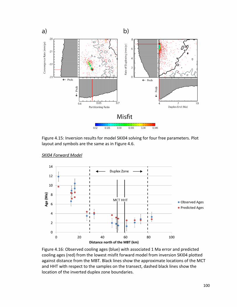
Figure 4.15: Inversion results for model SKI04 solving for four free parameters. Plot layout and symbols are the same as in Figure 4.6. SKI04 Forward Model
Figure 4.16: Observed cooling ages (blue) with associated 1 Ma error and predicted cooling ages (red) from the lowest misfit forward model from inversion SKI04 plotted against distance from the MBT. Black lines show the approximate locations of the MCT and HHT with respect to the samples on the transect, dashed black lines show the location of the inverted duplex zone boundaries.
100
The forward model age comparison (Figure 4.16) shows that, even with 8 Ma of
duplexing at a relatively high rate of 7 mm/yr, the model has difficulty reproducing the
younger ages in the center of the model without providing ages that are too young for
the rest of the data. The thermal and velocity fields (Figure 4.17), which were once again
split into two time frames of 12-4 Ma and 4-0 Ma, show significant vertical perturbations
within the duplex zone during its active time frame (Figure 4.17a). However, within the 4
Ma that follows the thermal footprint of this perturbation is essentially erased by the
influence of surface cooling (Figure 4.17b).
The results of SKI04 suggest that even 8 Ma of duplexing may not be enough to
reproduce the age pattern seen at the surface today, even if the rate of duplexing is
reasonable within the bounds of the model. From models SKI02, SKI03 and SKI04 it
appears that the closer to present we allow the duplex to run, the better the modelled
runs fit the data.
101
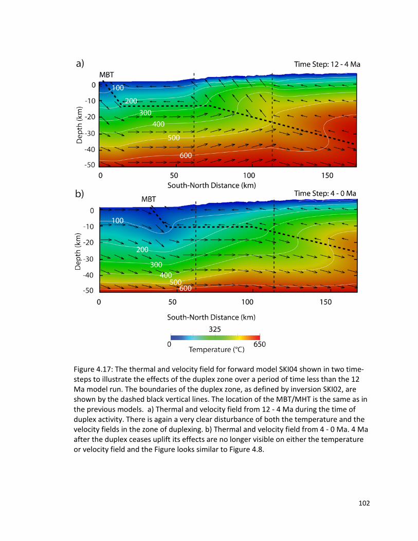
Figure 4.17: The thermal and velocity field for forward model SKI04 shown in two time-steps to illustrate the effects of the duplex zone over a period of time less than the 12 Ma model run. The boundaries of the duplex zone, as defined by inversion SKI02, are shown by the dashed black vertical lines. The location of the MBT/MHT is the same as in the previous models. a) Thermal and velocity field from 12 - 4 Ma during the time of duplex activity. There is again a very clear disturbance of both the temperature and the velocity fields in the zone of duplexing. b) Thermal and velocity field from 4 - 0 Ma. 4 Ma after the duplex ceases uplift its effects are no longer visible on either the temperature or velocity field and the Figure looks similar to Figure 4.8.
102
Chapter 5 – Discussion and Conclusions
The goal of this study was to use low temperature thermochronological data
(ZHe) coupled with 3D thermokinematic modelling to test different scenarios regarding
the tectonic evolution of the Sikkim Himalaya during the last 12 Ma. The observed ZHe
cooling age pattern in Sikkim shows an abrupt decrease in ages coinciding with the
southern boundary of the Rangit window and hypothesized duplex location in the
subsurface (Figure 3.6). Cooling ages continue to get gradually younger northwards until
the profile crosses the MCT and HHT into the GHS and the ages begin to increase
gradually. In the following section I review the preferred tectonic models based on the
goodness of fit with observed cooling age patterns and discuss possible limitations to
the interpretations.
5.1 - Tectonic Models for the Sikkim Himalaya
The first tectonic model tested in inversion SKI01 involves only displacement on a
geometrically variable MHT (Figure 4.8). While this inversion produced a predicted age
pattern with an acceptably low misfit value (0.419), the model had difficulty reproducing
the younger ages observed in the center of the transect within the Rangit/Tista windows
(Figure 4.7). This observation suggests that thrust motion alone along the MHT is
insufficient to advect crustal heat from depth to produce the observed age pattern and
that, if we hold to the hypothesis that the cooling age pattern is primarily driven by
tectonic processes, then there must be another tectonic mechanism at play.
The preferred model on the basis of the lowest misfit (0.236) is the tectonic
scenario tested in inversion SKI02 which introduces a zone of enhanced uplift that
103
simulates the effects of a duplex (vertical accretion) in the upper crust beneath the
Rangit/Tista windows, coupled with thrusting displacement on the MHT (Figure 4.11).
The lowest-misfit model predicts an overthrusting rate of ~8 mm/yr along the MHT
coupled with a rate of duplex-driven rock uplift of ~2.5 mm/yr from 12 Ma to present.
The distribution of observed cooling ages is very well reproduced by predicted ages
including the abrupt drop in cooling age within the duplex zone (Figure 4.10).
These results are comparable with the results obtained by Herman et al. (2010)
for a duplex-related model in central Nepal. Their models yielded best-fit overthrusting
rates of 4.4-6.8 mm/yr, which is slightly slower than the ~8 mm/yr predicted from my
best fit model in Sikkim, and a duplex uplift rate of 3 ± 0.9 mm/yr, within error identical
to the predicted rate of ~2.5 mm/yr. One of the major differences between my model
and that of Herman et al. (2010) is the location of the duplex along the MHT. In this
study, the duplex zone was placed based on the surface location of the Rangit/Tista
windows, the zone that defines the abrupt drop in cooling age. This resulted in a duplex
zone mostly located on a flat portion of the MHT (Figure 4.5). In contrast, Herman et al.
(2010) placed the zone of localized rock uplift entirely on a ramp section of the MHT
(Figure 15b in Herman et al., 2010). The interpretive cross-section of the duplex in
Sikkim produced by Bhattacharrya and Mitra (2009) includes a small crustal ramp within
the zone of duplexing (Figure 2.2) which may have added an increased vertical velocity
gradient to help produce the antiformal stacks in the Rangit Duplex. This ramp is not
imaged on the geophysical data used to define the geometry of the MHT, likely because
it is small compared to the two major ramps on the MHT, so it was not included in the
104
models. In the cross section from Mitra et al. (2010) the ramp drops down ~ 2km, less
than the 4 km vertical resolution on that section of the MHT in the geophysical data
(Acton et al. 2011), over a horizontal distance of ~4 km, resulting in a dip angle of ~27 °
(Figure 2.2). However, the excellent fit of the predicted ages of SKI02 to the observed
cooling pattern, especially in the duplex zone, suggests that the small ramp may have
played a role in the construction of the duplex.
The two models that we have run to explore an early end of duplexing (SKI03 and
SKI04) both resulted in unrealistically high duplex uplift rates (7-8 mm/yr) and larger
misfit values (0.323 - 0.446) compared to the best fit model.
5.2 - Modelled Exhumation Rates
Both the instantaneous exhumation rate over the transect length and the
average exhumation rate for each sample over the 12 Ma model interval were produced
from the T-t-paths calculated during the model run (Figure 5.1a). The instantaneous
exhumation rate, which corresponds to the near-surface vertical component of the
velocity field, shows the highest exhumation rates near the active MBT (~7 mm/yr) and
near the MCT/HHT (~5 mm/yr) because of the presence of crustal ramps in the
subsurface that locally produce an increased vertical velocity component. The vertical
accretion related to duplexing combines with that effect to maintain relatively high
instantaneous exhumation rates of 2.5 mm/yr above the long flat segment of the MHT.
The average exhumation rate (Figure 5.1a) for each sample is the amount of exhumation
between the depth at which the particle passes through its effective closure
temperature isotherm and the surface position of the sample, divided by the age of the
105

Figure 5.1: a) Instantaneous exhumation rate (blue line) within the model domain and average exhumation rate (red squares) experienced by each sample. b) Observed ZHe cooling ages (blue circles) with 1σ error plotted with average elevation (black solid line) and 1σ error (grey solid lines). Topographic profile is constructed from a DEM of Sikkim between 26.5 °N - 28 °N and 88 °E - 89 °E assembled from SRTM-90 m data (http://srtm.csi.cgiar.org/). c) Best fit tectonic model (SKI02) for Sikkim showing the geometry of the MHT and the area experiencing duplexing (grey transparent rectangle). All figures share the same x-axis. Major structures are denoted by the vertical dashed black lines.
106

sample (c.f., Figure 6b in Coutand et al., 2014). Average exhumation rates range
between 0.6-4.6 mm/yr. The pattern of average exhumation rates approximates a
mirror image of the pattern of cooling ages (Figure 5.1b), which is expected since a
higher exhumation rate (or cooling rate) should produce younger ages.
The Pecube models do not include the effects of surface processes because the
models are not coupled with a landscape-evolution model and topographic steady-state
has been assumed here. The rationale for this choice is that we have noticed that the
cooling ages do not correlate with the topography (Figures 3.7 and 5.1b). When plotted
along the topographic swath profile (Figure 5.1b), cooling ages get younger as elevation
increases until ~27.4 °N where the opposite occurs and cooling ages increase with
increasing elevation. These patterns are quite inconsistent as the largest change in
elevation occurs over a relatively flat section of the profile between 27-27.5 °N. When
the cooling ages are plotted directly against sample elevation (Figure 3.7), there is no
correlation between the two. This suggests that the modern topography, and by
extension surface processes, may not have exerted a major control on the distribution of
cooling ages along the range and that the distribution is more likely controlled by
tectonic effects.
5.3 - Comparison of Models along Strike of the Orogen
We compared our results to applications of the same approach as ours in Nepal,
eastern Bhutan and Arunachal Pradesh (Figure 5.2).
The westernmost transect (Figure 5.2A; Whipp et al., 2007) shows AFT ages
between 28 °N and 29°N within the Marsyandi Valley in central Nepal and surrounding
107
tributary valleys. The ages are all younger than 4 Ma and do not show any noticeable
trend along the main transect except that young ages (< 0.5 Ma) tend to occur at low
elevations near rivers (Whipp et al., 2007). In this study, two tectonic scenarios were
tested, one involving a simple displacement on the MHT over the past 20 Ma and a
second involving out-of-sequence thrusting (reactivation) of the MCT as well as motion
along the MHT, both active for 20 Ma. They found that the AFT data alone could not
distinguish between the two model types during the last ~3 Ma because models both
with and without the out-of-sequence MCT produced predicted cooling ages that fit the
observed data equally well within error. No single model was able to reproduce >80% of
the cooling age data which was suggested to be a result of a non-uniform erosion rate
over the model area. Modelling of ten shorter age transects within individual valleys
located within the larger study area produced exhumation rates of 1.8–5.0 mm/yr which
also suggests a variable erosion rate. The Marsyandi valley seems to be an unusual place
in the Himalaya, since there is no other place where such consistently young AFT ages
have been identified to date.
Transect B (Figure 5.2B) shows AFT ages from the Langtang Transect from Robert
et al. (2011). The general trend shows that the youngest ages are located north of the
MCT in the MCTZ (< 4 Ma) with a gradual increase southwards to a maximum of ~9 Ma
just north of the MBT. No significant offset in cooling ages is observed as the profile
crosses the MCT, suggesting that the structure was no longer active at the time these
samples crossed the effective closure temperature for the AFT chronometer. As for
Whipp et al. (2007), the tectonic scenarios tested could not distinguish between models
108
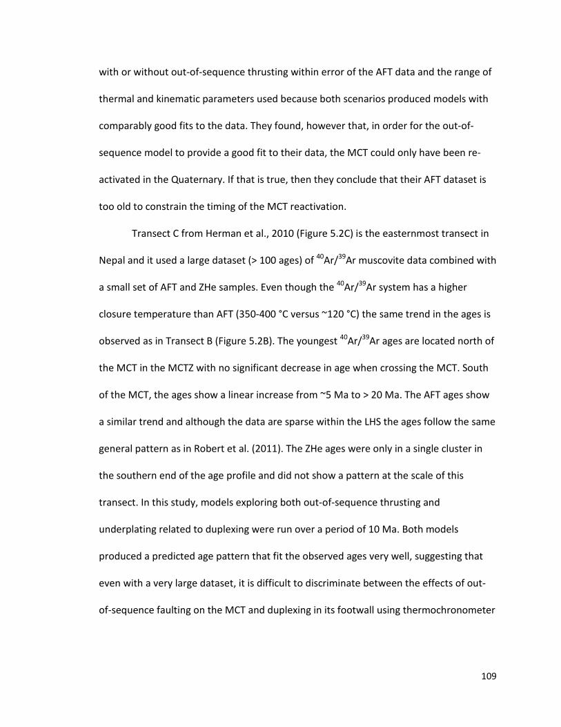
with or without out-of-sequence thrusting within error of the AFT data and the range of
thermal and kinematic parameters used because both scenarios produced models with
comparably good fits to the data. They found, however that, in order for the out-of-
sequence model to provide a good fit to their data, the MCT could only have been re-
activated in the Quaternary. If that is true, then they conclude that their AFT dataset is
too old to constrain the timing of the MCT reactivation.
Transect C from Herman et al., 2010 (Figure 5.2C) is the easternmost transect in
Nepal and it used a large dataset (> 100 ages) of 40Ar/39Ar muscovite data combined with
a small set of AFT and ZHe samples. Even though the 40Ar/39Ar system has a higher
closure temperature than AFT (350-400 °C versus ~120 °C) the same trend in the ages is
observed as in Transect B (Figure 5.2B). The youngest 40Ar/39Ar ages are located north of
the MCT in the MCTZ with no significant decrease in age when crossing the MCT. South
of the MCT, the ages show a linear increase from ~5 Ma to > 20 Ma. The AFT ages show
a similar trend and although the data are sparse within the LHS the ages follow the same
general pattern as in Robert et al. (2011). The ZHe ages were only in a single cluster in
the southern end of the age profile and did not show a pattern at the scale of this
transect. In this study, models exploring both out-of-sequence thrusting and
underplating related to duplexing were run over a period of 10 Ma. Both models
produced a predicted age pattern that fit the observed ages very well, suggesting that
even with a very large dataset, it is difficult to discriminate between the effects of out-
of-sequence faulting on the MCT and duplexing in its footwall using thermochronometer
109
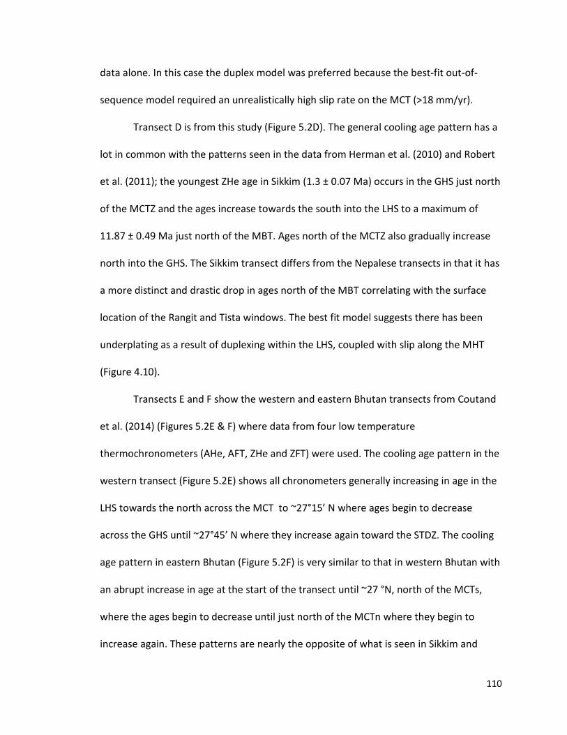
data alone. In this case the duplex model was preferred because the best-fit out-of-
sequence model required an unrealistically high slip rate on the MCT (>18 mm/yr).
Transect D is from this study (Figure 5.2D). The general cooling age pattern has a
lot in common with the patterns seen in the data from Herman et al. (2010) and Robert
et al. (2011); the youngest ZHe age in Sikkim (1.3 ± 0.07 Ma) occurs in the GHS just north
of the MCTZ and the ages increase towards the south into the LHS to a maximum of
11.87 ± 0.49 Ma just north of the MBT. Ages north of the MCTZ also gradually increase
north into the GHS. The Sikkim transect differs from the Nepalese transects in that it has
a more distinct and drastic drop in ages north of the MBT correlating with the surface
location of the Rangit and Tista windows. The best fit model suggests there has been
underplating as a result of duplexing within the LHS, coupled with slip along the MHT
(Figure 4.10).
Transects E and F show the western and eastern Bhutan transects from Coutand
et al. (2014) (Figures 5.2E & F) where data from four low temperature
thermochronometers (AHe, AFT, ZHe and ZFT) were used. The cooling age pattern in the
western transect (Figure 5.2E) shows all chronometers generally increasing in age in the
LHS towards the north across the MCT to ~27°15’ N where ages begin to decrease
across the GHS until ~27°45’ N where they increase again toward the STDZ. The cooling
age pattern in eastern Bhutan (Figure 5.2F) is very similar to that in western Bhutan with
an abrupt increase in age at the start of the transect until ~27 °N, north of the MCTs,
where the ages begin to decrease until just north of the MCTn where they begin to
increase again. These patterns are nearly the opposite of what is seen in Sikkim and
110

further west in Nepal where ages in the LHS decrease towards the MCT and then
increase to the north of it. Both transects produced models that fit the data well over
the past 12 Ma using only an MHT with variable geometry and no additional structures
such as duplexing or out-of-sequence faulting.
Transect G shows the data and best fit model from Adlakha et al. (2013) in
Arunachal Pradesh (Figure 5.2G). Here, AFT and ZFT samples were used in order to
discriminate whether out-of-sequence faulting played a role in the tectonic
development of Bhutan. The general AFT pattern is similar to that found in the transects
from Coutand et al. (2014) showing an increase in cooling age to the north from 20 km
south of the MCT followed by a decrease north of the MCT, through the GHS and a
klippe of TSS, until the end of the transect. The ZHe pattern is nearly identical except
there is no initial rise in ages to the south, only a smooth decline in ages north through
the transect. Three models were tested to attempt to reproduce the cooling age
patterns: one with only slip along the MHT, one with an out-of-sequence MCT active at
the beginning of the model and a third with a delayed onset of MCT re-activation. While
all models showed a generally good fit to the data, the best fit model was the delayed
re-activation model favoring an out-of-sequence MCT active between 6.5 Ma and 8.5
Ma.
111

Figure 5.2: Compilation of low temperature thermochronology data and tectonic models across the central and eastern Himalaya showing seven transects. From west to east: A) Whipp et al., 2007, B) Robert et al., 2011, C) Herman et al., 2010, D) this study, E) Coutand et al., 2014, F) Coutand et al., 2014 and G) Adlakha et al., 2013. Map from McQuarrie et al., 2008.
112
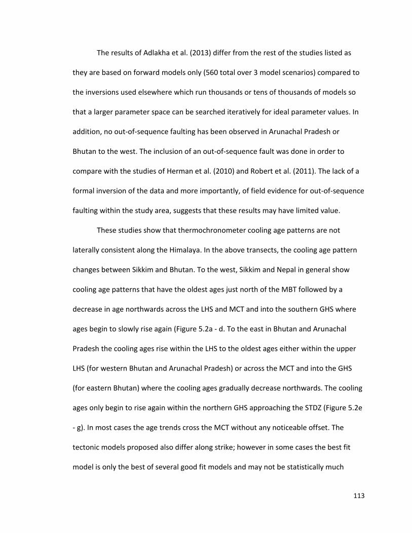
The results of Adlakha et al. (2013) differ from the rest of the studies listed as
they are based on forward models only (560 total over 3 model scenarios) compared to
the inversions used elsewhere which run thousands or tens of thousands of models so
that a larger parameter space can be searched iteratively for ideal parameter values. In
addition, no out-of-sequence faulting has been observed in Arunachal Pradesh or
Bhutan to the west. The inclusion of an out-of-sequence fault was done in order to
compare with the studies of Herman et al. (2010) and Robert et al. (2011). The lack of a
formal inversion of the data and more importantly, of field evidence for out-of-sequence
faulting within the study area, suggests that these results may have limited value.
These studies show that thermochronometer cooling age patterns are not
laterally consistent along the Himalaya. In the above transects, the cooling age pattern
changes between Sikkim and Bhutan. To the west, Sikkim and Nepal in general show
cooling age patterns that have the oldest ages just north of the MBT followed by a
decrease in age northwards across the LHS and MCT and into the southern GHS where
ages begin to slowly rise again (Figure 5.2a - d. To the east in Bhutan and Arunachal
Pradesh the cooling ages rise within the LHS to the oldest ages either within the upper
LHS (for western Bhutan and Arunachal Pradesh) or across the MCT and into the GHS
(for eastern Bhutan) where the cooling ages gradually decrease northwards. The cooling
ages only begin to rise again within the northern GHS approaching the STDZ (Figure 5.2e
- g). In most cases the age trends cross the MCT without any noticeable offset. The
tectonic models proposed also differ along strike; however in some cases the best fit
model is only the best of several good fit models and may not be statistically much
113
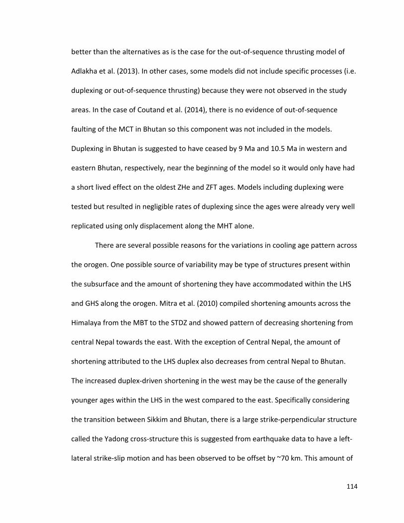
better than the alternatives as is the case for the out-of-sequence thrusting model of
Adlakha et al. (2013). In other cases, some models did not include specific processes (i.e.
duplexing or out-of-sequence thrusting) because they were not observed in the study
areas. In the case of Coutand et al. (2014), there is no evidence of out-of-sequence
faulting of the MCT in Bhutan so this component was not included in the models.
Duplexing in Bhutan is suggested to have ceased by 9 Ma and 10.5 Ma in western and
eastern Bhutan, respectively, near the beginning of the model so it would only have had
a short lived effect on the oldest ZHe and ZFT ages. Models including duplexing were
tested but resulted in negligible rates of duplexing since the ages were already very well
replicated using only displacement along the MHT alone.
There are several possible reasons for the variations in cooling age pattern across
the orogen. One possible source of variability may be type of structures present within
the subsurface and the amount of shortening they have accommodated within the LHS
and GHS along the orogen. Mitra et al. (2010) compiled shortening amounts across the
Himalaya from the MBT to the STDZ and showed pattern of decreasing shortening from
central Nepal towards the east. With the exception of Central Nepal, the amount of
shortening attributed to the LHS duplex also decreases from central Nepal to Bhutan.
The increased duplex-driven shortening in the west may be the cause of the generally
younger ages within the LHS in the west compared to the east. Specifically considering
the transition between Sikkim and Bhutan, there is a large strike-perpendicular structure
called the Yadong cross-structure this is suggested from earthquake data to have a left-
lateral strike-slip motion and has been observed to be offset by ~70 km. This amount of
114
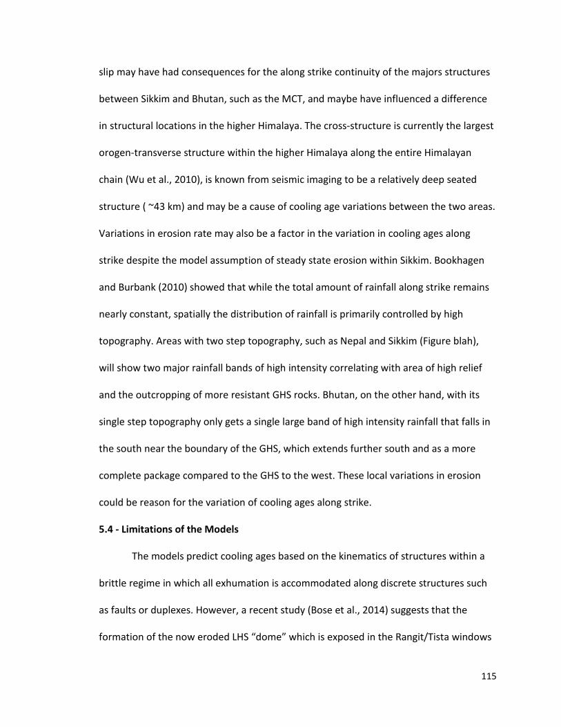
slip may have had consequences for the along strike continuity of the majors structures
between Sikkim and Bhutan, such as the MCT, and maybe have influenced a difference
in structural locations in the higher Himalaya. The cross-structure is currently the largest
orogen-transverse structure within the higher Himalaya along the entire Himalayan
chain (Wu et al., 2010), is known from seismic imaging to be a relatively deep seated
structure ( ~43 km) and may be a cause of cooling age variations between the two areas.
Variations in erosion rate may also be a factor in the variation in cooling ages along
strike despite the model assumption of steady state erosion within Sikkim. Bookhagen
and Burbank (2010) showed that while the total amount of rainfall along strike remains
nearly constant, spatially the distribution of rainfall is primarily controlled by high
topography. Areas with two step topography, such as Nepal and Sikkim (Figure blah),
will show two major rainfall bands of high intensity correlating with area of high relief
and the outcropping of more resistant GHS rocks. Bhutan, on the other hand, with its
single step topography only gets a single large band of high intensity rainfall that falls in
the south near the boundary of the GHS, which extends further south and as a more
complete package compared to the GHS to the west. These local variations in erosion
could be reason for the variation of cooling ages along strike.
5.4 - Limitations of the Models
The models predict cooling ages based on the kinematics of structures within a
brittle regime in which all exhumation is accommodated along discrete structures such
as faults or duplexes. However, a recent study (Bose et al., 2014) suggests that the
formation of the now eroded LHS “dome” which is exposed in the Rangit/Tista windows
115
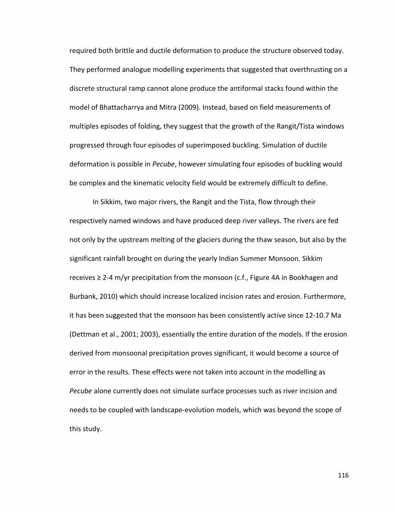
required both brittle and ductile deformation to produce the structure observed today.
They performed analogue modelling experiments that suggested that overthrusting on a
discrete structural ramp cannot alone produce the antiformal stacks found within the
model of Bhattacharrya and Mitra (2009). Instead, based on field measurements of
multiples episodes of folding, they suggest that the growth of the Rangit/Tista windows
progressed through four episodes of superimposed buckling. Simulation of ductile
deformation is possible in Pecube, however simulating four episodes of buckling would
be complex and the kinematic velocity field would be extremely difficult to define.
In Sikkim, two major rivers, the Rangit and the Tista, flow through their
respectively named windows and have produced deep river valleys. The rivers are fed
not only by the upstream melting of the glaciers during the thaw season, but also by the
significant rainfall brought on during the yearly Indian Summer Monsoon. Sikkim
receives ≥ 2-4 m/yr precipitation from the monsoon (c.f., Figure 4A in Bookhagen and
Burbank, 2010) which should increase localized incision rates and erosion. Furthermore,
it has been suggested that the monsoon has been consistently active since 12-10.7 Ma
(Dettman et al., 2001; 2003), essentially the entire duration of the models. If the erosion
derived from monsoonal precipitation proves significant, it would become a source of
error in the results. These effects were not taken into account in the modelling as
Pecube alone currently does not simulate surface processes such as river incision and
needs to be coupled with landscape-evolution models, which was beyond the scope of
this study.
116
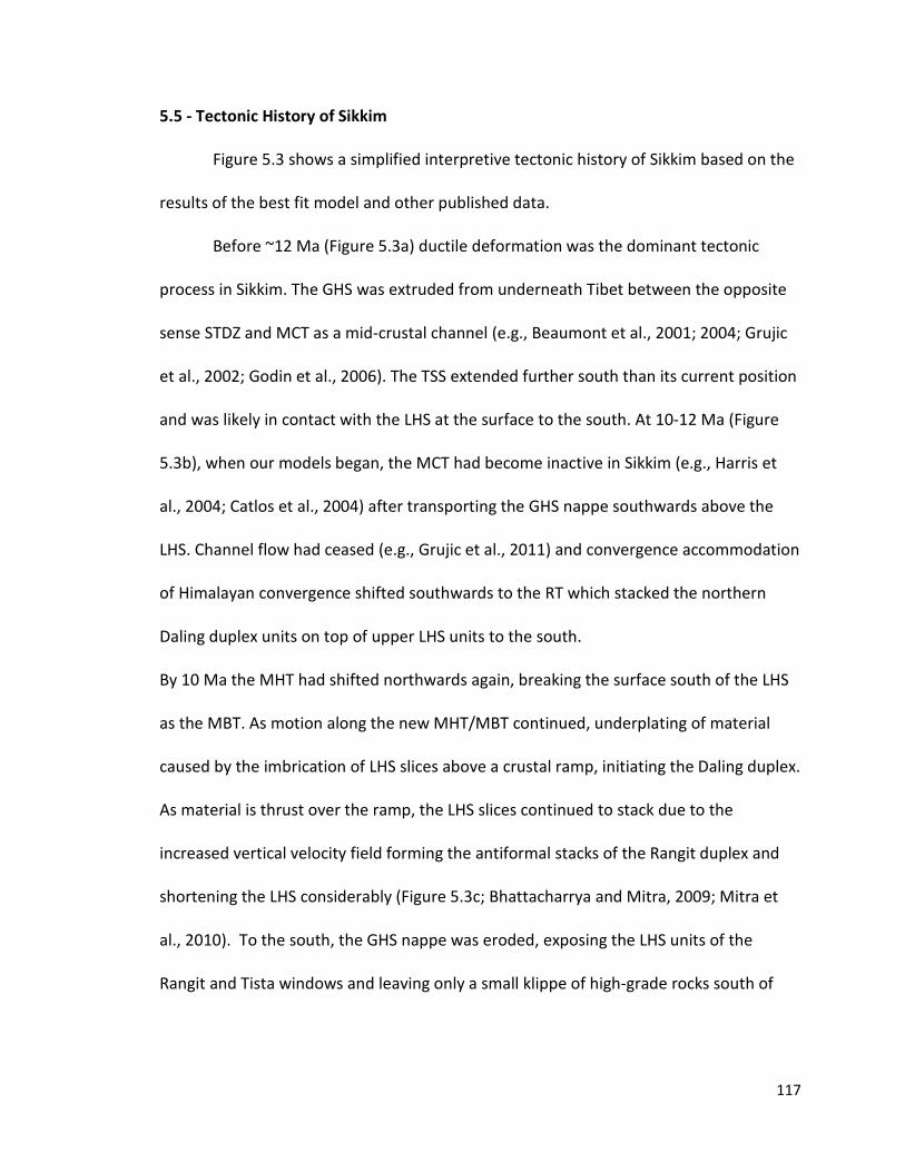
5.5 - Tectonic History of Sikkim
Figure 5.3 shows a simplified interpretive tectonic history of Sikkim based on the
results of the best fit model and other published data.
Before ~12 Ma (Figure 5.3a) ductile deformation was the dominant tectonic
process in Sikkim. The GHS was extruded from underneath Tibet between the opposite
sense STDZ and MCT as a mid-crustal channel (e.g., Beaumont et al., 2001; 2004; Grujic
et al., 2002; Godin et al., 2006). The TSS extended further south than its current position
and was likely in contact with the LHS at the surface to the south. At 10-12 Ma (Figure
5.3b), when our models began, the MCT had become inactive in Sikkim (e.g., Harris et
al., 2004; Catlos et al., 2004) after transporting the GHS nappe southwards above the
LHS. Channel flow had ceased (e.g., Grujic et al., 2011) and convergence accommodation
of Himalayan convergence shifted southwards to the RT which stacked the northern
Daling duplex units on top of upper LHS units to the south.
By 10 Ma the MHT had shifted northwards again, breaking the surface south of the LHS
as the MBT. As motion along the new MHT/MBT continued, underplating of material
caused by the imbrication of LHS slices above a crustal ramp, initiating the Daling duplex.
As material is thrust over the ramp, the LHS slices continued to stack due to the
increased vertical velocity field forming the antiformal stacks of the Rangit duplex and
shortening the LHS considerably (Figure 5.3c; Bhattacharrya and Mitra, 2009; Mitra et
al., 2010). To the south, the GHS nappe was eroded, exposing the LHS units of the
Rangit and Tista windows and leaving only a small klippe of high-grade rocks south of
117
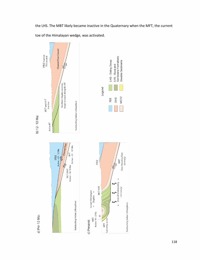
the LHS. The MBT likely became inactive in the Quaternary when the MFT, the current
toe of the Himalayan wedge, was activated.
118

Figure 5.3: A simplified schematic model showing the proposed tectonic evolution of Sikkim in three stages. Thick black lines show the active structures during each stage. a) Pre-model conditions dominated by ductile deformation (channel flow), b) conditions at the beginning of the model with convergence being transferred from the MCT to the RT and then to the MBT and the beginning of duplexing, and c) present day tectonic configuration. Modified from Mitra et al., 2010. 5.6 - Conclusions
Across the Himalayan range front in Sikkim, the analysis of 15 new zircon (U-Th)/He
in situ bedrock samples, combined with 3D thermokinematic modelling allowed us to
draw the following conclusions:
1) The samples collected produced cooling ages ranging from 1.30 ± 0.07 Ma to
11.87 ± 0.49 Ma. The NS-trending cooling age profile shows that the oldest ages,
located immediately north of the MBT, record an abrupt decrease northwards,
near the southern boundary of the Rangit/Tista window with ages beginning to
slightly increase again north of the MCTZ.
2) Age trends do not correlate with modern topography suggesting that tectonic
processes are the dominant control on the cooling age pattern.
3) Inversion results for the first scenario (SKI01) suggest that thrust motion of the
MHT alone is unable to reproduce the observed cooling age pattern to an
acceptable degree and thus cannot be the sole structural control on the tectonic
development of the Sikkim range front during the last 12 Ma.
4) In the second scenario, the addition of a ~ 50 km long zone of enhanced vertical
uplift active for 12 Ma at 2.5 mm/yr, coupled with a MHT overthrusting rate of ~8
mm/yr, results in a predicted age pattern that is nearly identical to the observed
age pattern.
119

5) The proposed tectonic model for the development of Sikkim during the last 12
Ma includes convergence accommodated by a basal thrust with a ramp-and-flat
geometry coupled with a localized zone of accretion, active for the past 12 Ma,
simulating rock uplift associated with the development of a duplex system within
the Lesser Himalaya.
120
References
Acharyya, S. K., & Ray, K. K. (1977). Geology of the Darjeeling–Sikkim Himalaya.
Guide to Excursion No. 3. In Fourth International Gondwana Symposium (Calcutta).
Geological Survey of India (pp. 1-25).
Acton, C. E., Priestley, K., Mitra, S., & Gaur, V. K. (2011). Crustal structure of the
Darjeeling-Sikkim Himalaya and southern Tibet. Geophysical Journal
International, 184(2), 829-852.
Adlakha, V., Lang, K. A., Patel, R. C., Lal, N., & Huntington, K. W. (2013). Rapid
long-term erosion in the rain shadow of the Shillong Plateau, Eastern
Himalaya.Tectonophysics, 582, 76-83.
Alsdorf, D., Makovsky, Y., Zhao, W., Brown, L. D., Nelson, K. D., Klemperer, S., ...
& Kuo, J. (1998). INDEPTH (International Deep Profiling of Tibet and the Himalaya:
multichannel seismic reflection data: description and availability. .Journal of Geophysical
Research: Solid Earth (1978–2012), 103(B11), 26993-26999.
Attendorn, H. G., & Bowen, R. (1988). Isotopes in the earth sciences. Springer.
(p.109).
Avouac, J. P. (2003). Mountain building, erosion, and the seismic cycle in the
Nepal Himalaya. Advances in Geophysics, 46, 1-80.
Banerjee, P., Bürgmann, R., Nagarajan, B., & Apel, E. (2008). Intraplate
deformation of the Indian subcontinent. Geophysical Research Letters, 35(18).
Beardsmore, G. R., & Cull, J. P. (2001). Crustal heat flow: a guide to measurement
and modelling. Cambridge University Press, 23-24.
121
Beaumont, C., Jamieson, R. A., Nguyen, M. H., & Lee, B. (2001). Himalayan
tectonics explained by extrusion of a low-viscosity crustal channel coupled to focused
surface denudation. Nature, 414(6865), 738-742.
Beaumont, C., Jamieson, R. A., Nguyen, M. H., & Medvedev, S. (2004). Crustal
channel flows: 1. Numerical models with applications to the tectonics of the Himalayan-
Tibetan orogen. Journal of Geophysical Research: Solid Earth (1978–2012), 109(B6).
Berger, A., Jouanne, F., Hassani, R., & Mugnier, J. L. (2004). Modelling the spatial
distribution of present-day deformation in Nepal: how cylindrical is the Main Himalayan
Thrust in Nepal?. Geophysical Journal International, 156(1), 94-114.
Berthet, T., Ritz, J. F., Ferry, M., Pelgay, P., Cattin, R., Drukpa, D., ... & Hetényi, G.
(2014). Active tectonics of the eastern Himalaya: New constraints from the first tectonic
geomorphology study in southern Bhutan. Geology, 42(5), 427-430.
Besse, J., Courtillot, V., Pozzi, J. P., Westphal, M., & Zhou, Y. X. (1984).
Palaeomagnetic estimates of crustal shortening in the Himalayan thrusts and Zangbo
suture.
Bettinelli, P., Avouac, J. P., Flouzat, M., Jouanne, F., Bollinger, L., Willis, P., &
Chitrakar, G. R. (2006). Plate motion of India and interseismic strain in the Nepal
Himalaya from GPS and DORIS measurements. Journal of Geodesy,80(8-11), 567-589.
Bhattacharyya, K., & Mitra, G. (2009). A new kinematic evolutionary model for
the growth of a duplex—an example from the Rangit duplex, Sikkim Himalaya,
India. Gondwana Research, 16(3), 697-715.
122
Bilham, R., Larson, K., Freymueller, J., Jouanne, F., LeFort, P., Leturmy, P., ... & de
Voogd, B. (1997). GPS measurements of present-day convergence across the Nepal
Himalaya. Nature, 386(6620), 61-64.
Bollinger, L., Avouac, J. P., Beyssac, O., Catlos, E. J., Harrison, T. M., Grove, M., ...
& Sapkota, S. (2004). Thermal structure and exhumation history of the Lesser Himalaya
in central Nepal. Tectonics, 23(5).
Bollinger, L., Henry, P., & Avouac, J. P. (2006). Mountain building in the Nepal
Himalaya: Thermal and kinematic model. Earth and Planetary Science Letters, 244(1), 58-
71.
Bookhagen, B., & Burbank, D. W. (2010). Toward a complete Himalayan
hydrological budget: Spatiotemporal distribution of snowmelt and rainfall and their
impact on river discharge. Journal of Geophysical Research: Earth Surface (2003–
2012), 115(F3).
Bose, S., Mandal, N., Acharyya, S. K., Ghosh, S., & Saha, P. (2014). Orogen-
transverse tectonic window in the Eastern Himalayan fold belt: A superposed buckling
model. Journal of Structural Geology, 66, 24-41.
Braun, J. (2002). Quantifying the effect of recent relief changes on age–elevation
relationships. Earth and Planetary Science Letters, 200(3), 331-343.
Braun, J. (2003). Pecube: A new finite-element code to solve the 3D heat
transport equation including the effects of a time-varying, finite amplitude surface
topography. Computers & Geosciences, 29(6), 787-794.
123

Braun, J. (2005). Quantitative constraints on the rate of landform evolution
derived from low-temperature thermochronology. Reviews in Mineralogy and
Geochemistry, 58(1), 351-374.
Braun, Jean; Peter van der Beek; Geoffrey Batt (2006). Quantitative
Thermochronology: Numerical Methods for the Interpretation of Thermochronological
Data. Cambridge: Cambridge University Press. pp. 24–27
Braun, J., Van Der Beek, P., Valla, P., Robert, X., Herman, F., Glotzbach, C., ... &
Prigent, C. (2012). Quantifying rates of landscape evolution and tectonic processes by
thermochronology and numerical Modelling of crustal heat transport using
PECUBE. Tectonophysics, 524, 1-28.
Burbank, D. W., Leland, J., Fielding, E., Anderson, R. S., Brozovic, N., Reid, M. R., &
Duncan, C. (1996). Bedrock incision, rock uplift and threshold hillslopes in the
northwestern Himalayas. Nature, 379(6565), 505-510.
Burchfiel, B. C., & Royden, L. H. (1985). North-south extension within the
convergent Himalayan region. Geology, 13(10), 679-682.
Burchfiel, B. C., Zhiliang, C., Hodges, K. V., Yuping, L., Royden, L. H., Changrong,
D., & Jiene, X. (1992). The South Tibetan detachment system, Himalayan orogen:
Extension contemporaneous with and parallel to shortening in a collisional mountain
belt. Geological Society of America Special Papers, 269, 1-41.
Burg, J. P., & Chen, G. M. (1984). Tectonics and structural zonation of southern
Tibet, China.
124
Burg, J. P., Nievergelt, P., Oberli, F., Seward, D., Davy, P., Maurin, J. C., ... &
Meier, M. (1998). The Namche Barwa syntaxis: evidence for exhumation related to
compressional crustal folding. Journal of Asian Earth Sciences, 16(2), 239-252.
Catlos, E. J., Dubey, C. S., Harrison, T. M., & Edwards, M. A. (2004). Late Miocene
movement within the Himalayan Main Central Thrust shear zone, Sikkim, north-east
India. Journal of Metamorphic geology, 22(3), 207-226.
Catlos, E. J., Dubey, C. S., Marston, R. A., & Harrison, T. M. (2007).
Geochronologic constraints across the main central thrust shear zone, Bhagirathi River
(NW India): Implications for Himalayan tectonics. Geological Society of America Special
Papers, 419, 135-151.
Clark, M. K. (2012). Continental collision slowing due to viscous mantle
lithosphere rather than topography. Nature, 483(7387), 74-77.
Consultative Group on International Agricultural Research - Consortium for
Spatial Information (CGIAR-CSI) - (http://srtm.csi.cgiar.org/).
Coutand, I., Whipp, D. M., Grujic, D., Bernet, M., Fellin, M. G., Bookhagen, B., ... &
Duncan, C. (2014). Geometry and kinematics of the Main Himalayan Thrust and Neogene
crustal exhumation in the Bhutanese Himalaya derived from inversion of
multithermochronologic data. Journal of Geophysical Research: Solid Earth, 119(2),
1446-1481.
Dahlen, F. A. (1990). Critical taper model of fold-and-thrust belts and
accretionary wedges. Annual Review of Earth and Planetary Sciences, 18, 55.
125
Daniel, C. G., Hollister, L. S., Parrish, R. T., & Grujic, D. (2003). Exhumation of the
Main Central Thrust from lower crustal depths, eastern Bhutan Himalaya. Journal of
Metamorphic Geology, 21(4), 317-334.
Dasgupta, S., Ganguly, J., & Neogi, S. (2004). Inverted metamorphic sequence in
the Sikkim Himalayas: crystallization history, P–T gradient and implications. Journal of
Metamorphic Geology, 22(5), 395-412.
Dasgupta, S., Chakraborty, S., & Neogi, S. (2009). Petrology of an inverted
Barrovian sequence of metapelites in Sikkim Himalaya, India: constraints on the
tectonics of inversion. American Journal of Science, 309(1), 43-84.
Davis, D., Suppe, J., & Dahlen, F. A. (1983). Mechanics of fold-and-thrust belts
and accretionary wedges. Journal of Geophysical Research: Solid Earth (1978–
2012), 88(B2), 1153-1172.
De, R., & Kayal, J. R. (2003). Seismotectonic model of the Sikkim Himalaya:
Constraint from microearthquake surveys. Bulletin of the Seismological Society of
America, 93(3), 1395-1400.
DeCelles, P. G., & Mitra, G. (1995). History of the Sevier orogenic wedge in terms
of critical taper models, northeast Utah and southwest Wyoming.Geological Society of
America Bulletin, 107(4), 454-462.
DeCelles, P. G., Gehrels, G. E., Quade, J., & Ojha, T. P. (1998). Eocene-early
Miocene foreland basin development and the history of Himalayan thrusting, western
and central Nepal. Tectonics, 17(5), 741-765.
126
DeCelles, P. G., Robinson, D. M., Quade, J., Ojha, T. P., Garzione, C. N., Copeland,
P., & Upreti, B. N. (2001). Stratigraphy, structure, and tectonic evolution of the
Himalayan fold-thrust belt in western Nepal. Tectonics, 20(4), 487-509.
Dodson, M. H. (1973). Closure temperature in cooling geochronological and
petrological systems. Contributions to Mineralogy and Petrology, 40(3), 259-274.
Duncan, C., Masek, J., & Fielding, E. (2003). How steep are the Himalaya?
Characteristics and implications of along-strike topographic variations. Geology,31(1),
75-78.
Edwards, M. A., & Harrison, T. M. (1997). When did the roof collapse? Late
Miocene north-south extension in the high Himalaya revealed by Th-Pb monazite dating
of the Khula Kangri granite. Geology, 25(6), 543-546.
Ehlers, T. A., & Farley, K. A. (2003). Apatite (U–Th)/He thermochronometry:
methods and applications to problems in tectonic and surface processes. Earth and
Planetary Science Letters, 206(1), 1-14.
Ehlers, T. A. (2005). Crustal thermal processes and the interpretation of
thermochronometer data. Reviews in Mineralogy and Geochemistry, 58(1), 315-350.
England, P., & Molnar, P. (1990). Surface uplift, uplift of rocks, and exhumation of
rocks. Geology, 18(12), 1173-1177.
England, P., Le Fort, P., Molnar, P., & Pêcher, A. (1992). Heat sources for Tertiary
metamorphism and anatexis in the Annapurna-Manaslu Region central Nepal.Journal of
Geophysical Research: Solid Earth (1978–2012), 97(B2), 2107-2128.
127
Farley, K. A., Wolf, R. A., & Silver, L. T. (1996). The effects of long alpha-stopping
distances on (U- Th)/He ages. Geochimica et Cosmochimica Acta, 60(21), 4223-4229.
Farley, K. A. (2002). (U-Th)/He dating: Techniques, calibrations, and
applications.Reviews in Mineralogy and Geochemistry, 47(1), 819-844.
Fellin, M.G. (2011). Personal communication.
Gaetani, M., & Garzanti, E. (1991). Multicyclic history of the Northern India
continental margin (Northwestern Himalaya) (1). AAPG Bulletin, 75(9), 1427-1446.
Ganguly, J., Dasgupta, S., Cheng, W., & Neogi, S. (2000). Exhumation history of a
section of the Sikkim Himalayas, India: records in the metamorphic mineral equilibria
and compositional zoning of garnet. Earth and Planetary Science Letters,183(3), 471-486.
Gansser, A. (1964). Geology of the Himalayas. (p.289). International Publishers,
London and New York.
Gansser, A. (1983) Geology of the Bhutan Himalaya, (p.181), Birkhauser Verlag.
Ghosh, A. K. (1968). Quantitative analysis of polymetallic orebody zoning at
Rangpo, Sikkim. Economic Geology, 63(6), 682-687.
Godin, L., Grujic, D., Law, R. D., & Searle, M. P. (2006). Channel flow, ductile
extrusion and exhumation in continental collision zones: an introduction. Geological
Society, London, Special Publications, 268(1), 1-23.
Grujic, D., Hollister, L. S., & Parrish, R. R. (2002). Himalayan metamorphic
sequence as an orogenic channel: insight from Bhutan. Earth and Planetary Science
Letters, 198(1), 177-191.
128
Grujic, D., Coutand, I., Bookhagen, B., Bonnet, S., Blythe, A., & Duncan, C. (2006).
Climatic forcing of erosion, landscape, and tectonics in the Bhutan
Himalayas. Geology, 34(10), 801-804.
Grujic, D., Warren, C. J., & Wooden, J. L. (2011). Rapid synconvergent
exhumation of Miocene-aged lower orogenic crust in the eastern
Himalaya.Lithosphere, 3(5), 346-366.
Harris, N., & Massey, J. (1994). Decompression and anatexis of Himalayan
metapelites. Tectonics, 13(6), 1537-1546.
Harris, N. B. W., Caddick, M., Kosler, J., Goswami, S., Vance, D., & Tindle, A. G.
(2004). The pressure–temperature–time path of migmatites from the Sikkim
Himalaya. Journal of Metamorphic Geology, 22(3), 249-264.
Hauck, M. L., Nelson, K. D., Brown, L. D., Zhao, W., & Ross, A. R. (1998). Crustal
structure of the Himalayan orogen at∼ 90 east longitude from Project INDEPTH deep
reflection profiles. Tectonics, 17(4), 481-500.
Herman, F., Copeland, P., Avouac, J. P., Bollinger, L., Mahéo, G., Le Fort, P., ... &
Henry, P. (2010). Exhumation, crustal deformation, and thermal structure of the Nepal
Himalaya derived from the inversion of thermochronological and thermobarometric
data and Modelling of the topography. Journal of Geophysical Research: Solid Earth
(1978–2012), 115(B6).
Hirschmiller, J., Grujic, D., Bookhagen, B., Coutand, I., Huyghe, P., Mugnier, J. L.,
& Ojha, T. (2014). What controls the growth of the Himalayan foreland fold-and-thrust
belt?. Geology, 42(3), 247-250.
129

Hodges, K. V., Parrish, R. R., Housh, T. B., Lux, D. R., Burchfiel, B. C., Royden, L. H.,
& Chen, Z. (1992). Simultaneous Miocene extension and shortening in the Himalayan
orogen. Science, 258(5087), 1466-1470.
Hodges, K. V., Parrish, R. R., & Searle, M. P. (1996). Tectonic evolution of the
central Annapurna range, Nepalese Himalayas. Tectonics, 15(6), 1264-1291.
Hodges, K. V. (2000). Tectonics of the Himalaya and southern Tibet from two
perspectives. Geological Society of America Bulletin, 112(3), 324-350.
Hodges, K. V., Wobus, C., Ruhl, K., Schildgen, T., & Whipple, K. (2004). Quaternary
deformation, river steepening, and heavy precipitation at the front of the Higher
Himalayan ranges. Earth and Planetary science letters, 220(3), 379-389.
Hourigan, J. K., Reiners, P. W., & Brandon, M. T. (2005). U-Th zonation-
dependent alpha-ejection in (U-Th)/He chronometry. Geochimica et Cosmochimica
Acta,69(13), 3349-3365.
Jade, S. (2004). Estimates of plate velocity and crustal deformation in the Indian
subcontinent using GPS geodesy. Current Science, 86(10), 1443-1448.
Jamieson, R. A., & Beaumont, C. (2013). On the origin of orogens. Geological
Society of America Bulletin, 125(11-12), 1671-1702.
Jouanne, F., Mugnier, J. L., Pandey, M. R., Gamond, J. F., Le Fort, P., Serrurier, L.,
... & Avouac, J. P. (1999). Oblique convergence in the Himalayas of western Nepal
deduced from preliminary results of GPS measurements. Geophysical Research
Letters, 26(13), 1933-1936.
130
Kellett, D. A., & Grujic, D. (2012). New insight into the South Tibetan detachment
system: Not a single progressive deformation. Tectonics, 31(2).
Kellett, D. A., Grujic, D., Coutand, I., Cottle, J., & Mukul, M. (2013). The South
Tibetan detachment system facilitates ultra rapid cooling of granulite-facies rocks in
Sikkim Himalaya. Tectonics, 32(2), 252-270..
Larson, K. M., Bürgmann, R., Bilham, R., & Freymueller, J. T. (1999). Kinematics of
the India-Eurasia collision zone from GPS measurements. Journal of Geophysical
Research: Solid Earth (1978–2012), 104(B1), 1077-1093.
Lavé, J., & Avouac, J. P. (2000). Active folding of fluvial terraces across the
Siwaliks Hills, Himalayas of central Nepal. Journal of Geophysical Research: Solid Earth
(1978–2012), 105(B3), 5735-5770.
Lavé, J., & Avouac, J. P. (2001). Fluvial incision and tectonic uplift across the
Himalayas of central Nepal. Journal of Geophysical Research: Solid Earth (1978–
2012), 106(B11), 26561-26591.
Le Fort, P. (1975). Himalayas: the collided range. Present knowledge of the
continental arc. Am. J. Sci, 275(1), 1-44.
Le Fort, P., Cuney, M., Deniel, C., France-Lanord, C., Sheppard, S. M. F., Upreti, B.
N., & Vidal, P. (1987). Crustal generation of the Himalayan
leucogranites.Tectonophysics, 134(1), 39-57.
Leloup, P. H., Mahéo, G., Arnaud, N., Kali, E., Boutonnet, E., Liu, D., ... & Haibing,
L. (2010). The South Tibet detachment shear zone in the Dinggye area: Time constraints
on extrusion models of the Himalayas. Earth and Planetary Science Letters, 292(1), 1-16.
131
Long, S., McQuarrie, N., Tobgay, T., Rose, C., Gehrels, G., & Grujic, D. (2011).
Tectonostratigraphy of the Lesser Himalaya of Bhutan: Implications for the along-strike
stratigraphic continuity of the northern Indian margin. Geological Society of America
Bulletin, 123(7-8), 1406-1426.
Macfarlane, A. M. (1995). An evaluation of the inverted metamorphic gradient at
Langtang National Park, central Nepal Himalaya. Journal of Metamorphic Geology,13(5),
595-612.
Makovsky, Y., Klemperer, S. L., Huang, L., & Lu, D. (1996). Structural elements of
the southern Tethyan Himalaya crust from wide-angle seismic data. Tectonics,15(5), 997-
1005.
Mancktelow, N. S., & Grasemann, B. (1997). Time-dependent effects of heat
advection and topography on cooling histories during erosion. Tectonophysics,270(3),
167-195.
Mancktelow, N. S., & Grasemann, B. (1997). Time-dependent effects of heat
advection and topography on cooling histories during erosion. Tectonophysics,270(3),
167-195.
McQuarrie, N., Robinson, D., Long, S., Tobgay, T., Grujic, D., Gehrels, G., & Ducea,
M. (2008). Preliminary stratigraphic and structural architecture of Bhutan: Implications
for the along strike architecture of the Himalayan system. Earth and Planetary Science
Letters, 272(1), 105-117.
Meesters, A. G. C. A., & Dunai, T. J. (2005). A noniterative solution of the (U-
Th)/He age equation. Geochemistry, Geophysics, Geosystems, 6(4).
132
Meigs, A. J., Burbank, D. W., & Beck, R. A. (1995). Middle-late Miocene (> 10 Ma)
formation of the Main Boundary thrust in the western Himalaya. Geology, 23(5), 423-
426.
Min, K., Farley, K. A., Renne, P. R., & Marti, K. (2003). Single grain (U–Th)/He ages
from phosphates in Acapulco meteorite and implications for thermal history. Earth and
Planetary Science Letters, 209(3), 323-336.
Mitra, G. (1997). Evolution of salients in a fold-and-thrust belt: the effects of
sedimentary basin geometry, strain distribution and critical taper. In Evolution of
Geological Structures in Micro-to Macro-scales (pp. 59-90). Springer Netherlands.
Mitra, G., Bhattacharyya, K., & Mukul, M. (2010). The Lesser Himalayan duplex in
Sikkim: Implications for variations in Himalayan shortening. Journal of the Geological
Society of India, 75(1), 289-301.
Mohan, A., Windley, B. F., & Searle, M. P. (1989). Geothermobarometry and
development of inverted metamorphism in the Darjeeling-Sikkim region of the eastern
Himalayan. Journal of Metamorphic Geology, 7(1), 95-110.
Molnar, P., & Stock, J. M. (2009). Slowing of India's convergence with Eurasia
since 20 Ma and its implications for Tibetan mantle dynamics. Tectonics, 28(3).
Mottram, C. M., Argles, T. W., Harris, N. B. W., Parrish, R. R., Horstwood, M. S. A.,
Warren, C. J., & Gupta, S. (2014). Tectonic interleaving along the Main Central Thrust,
Sikkim Himalaya. Journal of the Geological Society, 171(2), 255-268.
133
Mukul, M. (2000). The geometry and kinematics of the Main Boundary Thrust
and related neotectonics in the Darjiling Himalayan fold-and-thrust belt, West Bengal,
India. Journal of Structural Geology, 22(9), 1261-1283.
Mukul, M., Jaiswal, M., & Singhvi, A. K. (2007). Timing of recent out-of-sequence
active deformation in the frontal Himalayan wedge: Insights from the Darjiling sub-
Himalaya, India. Geology, 35(11), 999-1002.
Mukul, M. (2010). First-order kinematics of wedge-scale active Himalayan
deformation: Insights from Darjiling–Sikkim–Tibet (DaSiT) wedge. Journal of Asian Earth
Sciences, 39(6), 645-657.
Mukul, M., Jade, S., Bhattacharyya, A. K., & Bhusan, K. (2010). Crustal shortening
in convergent orogens: Insights from global positioning system (GPS) measurements in
northeast India. Journal of the Geological Society of India, 75(1), 302-312.
Mukul, M., Jade, S., Ansari, K., & Matin, A. (2014). Seismotectonic implications of
strike–slip earthquakes in the Darjiling–Sikkim Himalaya. Current Science, 106(2), 198-
210.
Nábělek, J., Hetényi, G., Vergne, J., Sapkota, S., Kafle, B., Jiang, M., ... & Huang, B.
S. (2009). Underplating in the Himalaya-Tibet collision zone revealed by the Hi-CLIMB
experiment. Science, 325(5946), 1371-1374.
Najman, Y. (2006). The detrital record of orogenesis: a review of approaches and
techniques used in the Himalayan sedimentary basins. Earth-Science Reviews,74(1), 1-
72.
Nelson, K. D., Zhao, W., Brown, L. D., Kuo, J., Che, J., Liu, X., ... & Edwards, M.
134
(1996). Partially molten middle crust beneath southern Tibet: synthesis of project
INDEPTH results. Science, 274(5293), 1684-1688.
Neogi, S., Dasgupta, S., & Fukuoka, M. (1998). High P–T polymetamorphism,
dehydration melting, and generation of migmatites and granites in the Higher Himalayan
Crystalline Complex, Sikkim, India. Journal of Petrology, 39(1), 61-99.
Pan, G., Ding, J., Yao, D. & Wang, L. (2004), Geological map of Qinghai-Xiang
(Tibet) plateau and adjacent areas (1:1,500,000), Chengdu Institute of Geology and
Mineral Resources, China Geological Survey, Chengdu Cartographic Publishing House,
Chengdu, China.
Parrish, R. R., & Hodges, V. (1996). Isotopic constraints on the age and
provenance of the Lesser and Greater Himalayan sequences, Nepalese
Himalaya. Geological Society of America Bulletin, 108(7), 904-911.
Patrait, M. R., & Achache, J. (1984). India-Eurasia collision chronology and its
implications for crustal shortening and driving mechanisms of the
plates.Nature, 311(18), 615-621.
Paul, D. K., McNaughton, N. J., Chattopadhyay, S., & Ray, K. K. (1996).
Geochronology and Geochemistry of the Lingtse Gneiss, Darjeeling-Sikkim Himalaya:
revisited. Journal of the Geological Society of India, 48(5), 497-506.
Pearson, O. N., & DeCelles, P. G. (2005). Structural geology and regional tectonic
significance of the Ramgarh thrust, Himalayan fold-thrust belt of Nepal. Tectonics,24(4).
135
Reiners, P. W., Farley, K. A., & Hickes, H. J. (2002). He diffusion and (U–Th)/He
thermochronometry of zircon: initial results from Fish Canyon Tuff and Gold
Butte.Tectonophysics, 349(1), 297-308.
Reiners, P. W., Spell, T. L., Nicolescu, S., & Zanetti, K. A. (2004). Zircon (U-Th)/He
thermochronometry: He diffusion and comparisons with 40Ar/39Ar dating. Geochimica et
Cosmochimica Acta, 68(8), 1857-1887.
Reiners, P. W. (2005). Zircon (U-Th)/He thermochronometry. Reviews in
Mineralogy and Geochemistry, 58(1), 151-179.
Reiners, P. W., & Brandon, M. T. (2006). Using thermochronology to understand
orogenic erosion. Annu. Rev. Earth Planet. Sci., 34, 419-466.
Reiners, P. W., & Nicolescu, S. (2006). Measurement of parent nuclides for (U-
Th)/He chronometry by solution sector ICP-MS. ARHDL Report 1. University of Arizona.
Rickwood, P., & Sambridge, M. (2006). Efficient parallel inversion using the
Neighbourhood Algorithm. Geochemistry, Geophysics, Geosystems, 7(11).
Robert, X., Van Der Beek, P., Braun, J., Perry, C., Dubille, M., & Mugnier, J. L.
(2009). Assessing Quaternary reactivation of the Main Central thrust zone (central Nepal
Himalaya): New thermochronologic data and numerical Modelling. Geology,37(8), 731-
734.
Robert, X., Van Der Beek, P., Braun, J., Perry, C., & Mugnier, J. L. (2011). Control
of detachment geometry on lateral variations in exhumation rates in the Himalaya:
Insights from low-temperature thermochronology and numerical Modelling. Journal of
Geophysical Research: Solid Earth (1978–2012), 116(B5).
136
Rubatto, D., Chakraborty, S., & Dasgupta, S. (2013). Timescales of crustal melting
in the Higher Himalayan Crystallines (Sikkim, Eastern Himalaya) inferred from trace
element-constrained monazite and zircon chronology. Contributions to Mineralogy and
Petrology, 165(2), 349-372.
Sambridge, M. (1999a). Geophysical inversion with a neighbourhood algorithm—
I. Searching a parameter space. Geophysical Journal International, 138(2), 479-494.
Sambridge, M. (1999b). Geophysical inversion with a neighbourhood algorithm—
II. Appraising the ensemble. Geophysical Journal International, 138(3), 727-746.
Schelling, D., & Arita, K. (1991). Thrust tectonics, crustal shortening, and the
structure of the far-eastern Nepal Himalaya. Tectonics, 10(5), 851-862.
Schelling, D. (1992). The tectonostratigraphy and structure of the eastern Nepal
Himalaya. Tectonics, 11(5), 925-943.
Schopf, J. W., Tewari, V. C., & Kudryavtsev, A. B. (2008). Discovery of a new
Chert-Permineralized Microbiota in the Proterozoic Buxa Formation of the Ranjit
window, Sikkim, northeast India, and its astrobiological implications. Astrobiology, 8(4),
735-746.
Schwan, W., & Saklani, P. S. (1980). Shortening structures in eastern and
northwestern Himalayan rocks (Vol. 3). Today and Tomorrow's Printers & Publishers.
Searle, M. P., Cooper, D. J. W., Rex, A. J., Herren, E., Rex, A. J., & Colchen, M.
(1988). Collision Tectonics of the Ladakh--Zanskar Himalaya [and
Discussion].Philosophical Transactions of the Royal Society of London. Series A,
Mathematical and Physical Sciences, 117-150.
137

Searle, M. P., & Rex, A. J. (1989). Thermal model for the Zanskar Himalaya.
Journal of Metamorphic Geology, 7(1), 127-134.
Searle, M. P., Simpson, R. L., Law, R. D., Parrish, R. R., & Waters, D. J. (2003). The
structural geometry, metamorphic and magmatic evolution of the Everest massif, High
Himalaya of Nepal–South Tibet. Journal of the Geological Society,160(3), 345-366.
Searle, M. P., & Szulc, A. G. (2005). Channel flow and ductile extrusion of the high
Himalayan slab-the Kangchenjunga–Darjeeling profile, Sikkim Himalaya. Journal of Asian
Earth Sciences, 25(1), 173-185.
Searle, M. P., Law, R. D., & Jessup, M. J. (2006). Crustal structure, restoration and
evolution of the Greater Himalaya in Nepal-South Tibet: implications for channel flow
and ductile extrusion of the middle crust. Geological Society, London, Special
Publications, 268(1), 355-378.
Segev, A. (2002). Flood basalts, continental breakup and the dispersal of
Gondwana: evidence for periodic migration of upwelling mantle flows (plumes).EGU
Stephan Mueller Special Publication Series, 2, 171-191.
Strutt, R. J. (1908). On the accumulation of helium in geological time. Proceedings
of the Royal Society of London. Series A, 81(547), 272-277.
Stüwe, Kurt, and Terence D. Barr. On uplift and exhumation during
convergence.Tectonics, 17.1 (1998): 80-88.
Tiwari, V. M., Vyghreswara Rao, M. B. S., Mishra, D. C., & Singh, B. (2006). Crustal
structure across Sikkim, NE Himalaya from new gravity and magnetic data. Earth and
Planetary Science Letters, 247(1), 61-69.
138
Urey, H. C. (1955). The cosmic abundances of potassium, uranium, and thorium
and the heat balances of the Earth, the Moon, and Mars. Proceedings of the National
Academy of Sciences of the United States of America, 41(3), 127.
Vermeesch, P. (2008). Three new ways to calculate average (U–Th)/He
ages.Chemical Geology, 249(3), 339-347.
Whipp, D. M., Ehlers, T. A., Blythe, A. E., Huntington, K. W., Hodges, K. V., &
Burbank, D. W. (2007). Plio-Quaternary exhumation history of the central Nepalese
Himalaya: 2. Thermokinematic and thermochronometer age prediction
model.Tectonics, 26(3).
Whipple, K. X., & Meade, B. J. (2006). Orogen response to changes in climatic and
tectonic forcing. Earth and Planetary Science Letters, 243(1), 218-228.
Whipple, K. X. (2009). The influence of climate on the tectonic evolution of
mountain belts. Nature Geoscience, 2(2), 97-104.
Willett, S. D., & Brandon, M. T. (2002). On steady states in mountain
belts. Geology,30(2), 175-178.
Wobus, C., Heimsath, A., Whipple, K., & Hodges, K. (2005). Active out-of-
sequence thrust faulting in the central Nepalese Himalaya. Nature, 434(7036), 1008-
1011.
Wolf, R. A., Farley, K. A., & Kass, D. M. (1998). Modelling of the temperature
sensitivity of the apatite (U–Th)/He thermochronometer. Chemical Geology, 148(1), 105-
114.
139
Wu, C., Nelson, K. D., Wortman, G., Samson, S. D., Yue, Y., Li, J., ... & Edwards, M.
A. (1998). Yadong cross structure and South Tibetan Detachment in the east central
Himalaya (89–90 E). Tectonics, 17(1), 28-45.
Zhang, H., Harris, N., Parrish, R., Kelley, S., Zhang, L., Rogers, N., ... & King, J.
(2004). Causes and consequences of protracted melting of the mid-crust exposed in the
North Himalayan antiform. Earth and Planetary Science Letters, 228(1), 195-212.
140
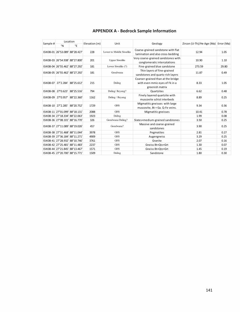
APPENDIX A - Bedrock Sample Information
°N °E
ISIK08-01 26°53.089' 88°28.427' 228Coarse-grained sandstone with flat lamination and also cross-bedding
12.94 1.05
ISIK08-03 26°54.938' 88°27.800' 201Very coarse-grained sandstones with
conglomeratic intercalations10.90 1.10
ISIK08-04 26°55.462' 88°27.292' 181 Fine-grained blue sandstone 273.59 29.80
ISIK08-05 26°55.462' 88°27.292' 181Thin layers of fine-grained
sandstones and quartz-rich layers 11.87 0.49
ISIK08-07 27°2.284' 88°25.612' 215Coarser-grained than at the bridge
with even mmic eyes of Fk in a greenish matrix
8.33 1.05
ISIK08-08 27°0.623' 88°25.516' 794 Quartzites 6.62 0.48
ISIK08-09 27°0.957' 88°22.360' 1162Finely layered quartzite with
muscovite schist interbeds8.89 0.25
ISIK08-10 27°2.285' 88°20.752' 1729Migmatitic gneisses with large
9.34 0.36
ISIK08-11 27°01.099' 88°18.131' 2088 Migmatitic gneisses 10.41 0.78ISIK08-34 27°18.334' 88°22.063' 1923 1.99 0.08ISIK08-36 27°08.101' 88°16.770' 326 3.50 0.25
ISIK08-37 27°11.089' 88°19.026' 457Massive and coarse-grained
sandstones3.90 0.25
ISIK08-38 27°31.468' 88°11.044' 3978 Pegmatites 2.81 0.27ISIK08-39 27°36.184' 88°11.271' 4909 Augengneiss 3.29 0.25ISIK08-41 27°28.932' 88°10.746' 3761 Granite 2.07 0.16ISIK08-42 27°25.481' 88°11.483' 2237 1.30 0.07ISIK08-44 27°21.845' 88°13.467' 1571 1.45 0.19ISIK08-45 27°20.700' 88°15.771' 1509 Sandstone 1.80 0.30
LocationSample # Elevation (m) Unit Geology Zircon (U-Th)/He Age (Ma) Error (Ma)
141

APPENDIX B - Contributions to the Thesis
Sample collection was performed by supervisor Dr. Isabelle Coutand in 2008 who
provided the sample descriptions, context and location information compiled in
Appendix A. Samples were collected in a profile perpendicular to the major structures in
Sikkim and crossing the windows. The profile followed the major river valleys up from
the Siwaliks in the south to base camp of Kangchenjunga. Crushing of approximately
half of the samples was performed by lab technician Matt Kliffer with the rest
performed by myself. I processed all of the samples through crystal isolation for zircons
and selected the zircons for analysis.
Degassing of 25 zircons was performed by noble gas technician Keith Taylor at
Dalhousie. The remaining degassing and all of the U-Th extraction was performed by me
under the supervision of Dr. Jeremy Hourigan at UCSC. The original model code for
Pecube was compiled by Jean Braun (Braun, 2003) and modified by Dr. David Whipp for
use in this study. All forward models were run using my personal computer and all
inversions were run using the Ace-net Glooscap computing cluster.
142