Embed Size (px)
Citation preview

NESSUS Users’ Manual
David Riha Barron Bichon John McFarland Simeon Fitch
August 11, 2015
Copyright c© 1998–2013 bySouthwest Research Institute
Contents
1 Overview 4
2 Getting Started 7
3 Problem Definition 83.1 Define Fault Tree . . . . . . . . . . . . . . . . . . . . . . . . . . . . . . . . . . . . . . . . . . . 93.2 Problem Statement . . . . . . . . . . . . . . . . . . . . . . . . . . . . . . . . . . . . . . . . . . 93.3 Random Variables . . . . . . . . . . . . . . . . . . . . . . . . . . . . . . . . . . . . . . . . . . 13
3.3.1 Correlations . . . . . . . . . . . . . . . . . . . . . . . . . . . . . . . . . . . . . . . . . . 153.3.2 Confidence Bounds . . . . . . . . . . . . . . . . . . . . . . . . . . . . . . . . . . . . . . 18
3.4 Response Models . . . . . . . . . . . . . . . . . . . . . . . . . . . . . . . . . . . . . . . . . . . 193.4.1 Regression . . . . . . . . . . . . . . . . . . . . . . . . . . . . . . . . . . . . . . . . . . . 20
Polynomial Regression Models . . . . . . . . . . . . . . . . . . . . . . . . . . . . . . . 20Gaussian Process Regression Model . . . . . . . . . . . . . . . . . . . . . . . . . . . . 21
3.4.2 Dynamically Linked . . . . . . . . . . . . . . . . . . . . . . . . . . . . . . . . . . . . . 223.4.3 Predefined . . . . . . . . . . . . . . . . . . . . . . . . . . . . . . . . . . . . . . . . . . . 233.4.4 Numerical . . . . . . . . . . . . . . . . . . . . . . . . . . . . . . . . . . . . . . . . . . . 23
Overview . . . . . . . . . . . . . . . . . . . . . . . . . . . . . . . . . . . . . . . . . . . 23Numerical Model Usage in NESSUS . . . . . . . . . . . . . . . . . . . . . . . . . . . . 24Create Mappings . . . . . . . . . . . . . . . . . . . . . . . . . . . . . . . . . . . . . . . 27Variable Mapping . . . . . . . . . . . . . . . . . . . . . . . . . . . . . . . . . . . . . . 29Response Selection . . . . . . . . . . . . . . . . . . . . . . . . . . . . . . . . . . . . . . 32
4 Deterministic Analysis 344.1 Overview . . . . . . . . . . . . . . . . . . . . . . . . . . . . . . . . . . . . . . . . . . . . . . . 344.2 Importing Data . . . . . . . . . . . . . . . . . . . . . . . . . . . . . . . . . . . . . . . . . . . . 36
5 Probabilistic Analysis 405.1 Analysis Type . . . . . . . . . . . . . . . . . . . . . . . . . . . . . . . . . . . . . . . . . . . . . 405.2 Analysis Data . . . . . . . . . . . . . . . . . . . . . . . . . . . . . . . . . . . . . . . . . . . . . 40
5.2.1 Specified Probability Levels . . . . . . . . . . . . . . . . . . . . . . . . . . . . . . . . . 405.2.2 Specified Performance Levels . . . . . . . . . . . . . . . . . . . . . . . . . . . . . . . . 435.2.3 Full Cumulative Distribution . . . . . . . . . . . . . . . . . . . . . . . . . . . . . . . . 435.2.4 Global Sensitivity . . . . . . . . . . . . . . . . . . . . . . . . . . . . . . . . . . . . . . 43
5.3 Analysis Methods . . . . . . . . . . . . . . . . . . . . . . . . . . . . . . . . . . . . . . . . . . . 435.3.1 Monte Carlo method (MONTE) . . . . . . . . . . . . . . . . . . . . . . . . . . . . . . 445.3.2 Latin Hypercube Simulation (LHS) . . . . . . . . . . . . . . . . . . . . . . . . . . . . . 45
Limitations . . . . . . . . . . . . . . . . . . . . . . . . . . . . . . . . . . . . . . . . . . 465.3.3 First- and Second-Order Reliability Methods (FORM and SORM) . . . . . . . . . . . 46
Limitations . . . . . . . . . . . . . . . . . . . . . . . . . . . . . . . . . . . . . . . . . . 465.3.4 Mean Value methods (MV, AMV, AMV+) . . . . . . . . . . . . . . . . . . . . . . . . 46
Limitations . . . . . . . . . . . . . . . . . . . . . . . . . . . . . . . . . . . . . . . . . . 47
1
5.3.5 Curvature-based adaptive importance sampling with advanced mean value MPP search(AMV AIS) . . . . . . . . . . . . . . . . . . . . . . . . . . . . . . . . . . . . . . . . . . 47
5.3.6 Importance sampling w/radius reduction factor (ISAMF) . . . . . . . . . . . . . . . . 495.3.7 Importance sampling w/user-defined radius (ISAMR) . . . . . . . . . . . . . . . . . . 495.3.8 Importance sampling at user-defined MPP (ISMPP) . . . . . . . . . . . . . . . . . . . 505.3.9 Plane-based adaptive importance sampling (AIS1) . . . . . . . . . . . . . . . . . . . . 505.3.10 Curvature-based adaptive importance sampling (AIS2) . . . . . . . . . . . . . . . . . . 505.3.11 Efficient Global Reliability Analysis (EGRA) . . . . . . . . . . . . . . . . . . . . . . . 51
Limitations . . . . . . . . . . . . . . . . . . . . . . . . . . . . . . . . . . . . . . . . . . 525.3.12 Response Surface Method (RSM) . . . . . . . . . . . . . . . . . . . . . . . . . . . . . . 525.3.13 Gaussian Process Response Surface Method (RSM GP) . . . . . . . . . . . . . . . . . 535.3.14 Variance Decomposition (VARDCMP) . . . . . . . . . . . . . . . . . . . . . . . . . . . 53
6 Results Visualization 556.1 Overview . . . . . . . . . . . . . . . . . . . . . . . . . . . . . . . . . . . . . . . . . . . . . . . 556.2 Deterministic Results . . . . . . . . . . . . . . . . . . . . . . . . . . . . . . . . . . . . . . . . . 556.3 Probabilistic Analysis Results Visualization . . . . . . . . . . . . . . . . . . . . . . . . . . . . 576.4 Global Sensitivity Results . . . . . . . . . . . . . . . . . . . . . . . . . . . . . . . . . . . . . . 586.5 Chart Formatting Controls . . . . . . . . . . . . . . . . . . . . . . . . . . . . . . . . . . . . . 586.6 Viewing Analysis Files . . . . . . . . . . . . . . . . . . . . . . . . . . . . . . . . . . . . . . . . 58
7 System Requirements 617.1 Installation . . . . . . . . . . . . . . . . . . . . . . . . . . . . . . . . . . . . . . . . . . . . . . 61
7.1.1 Unix Platforms . . . . . . . . . . . . . . . . . . . . . . . . . . . . . . . . . . . . . . . . 617.1.2 Microsoft Windows . . . . . . . . . . . . . . . . . . . . . . . . . . . . . . . . . . . . . . 61
7.2 Distribution Structure . . . . . . . . . . . . . . . . . . . . . . . . . . . . . . . . . . . . . . . . 617.3 External Analysis Packages . . . . . . . . . . . . . . . . . . . . . . . . . . . . . . . . . . . . . 62
7.3.1 ABAQUS (cf. Section B.1) . . . . . . . . . . . . . . . . . . . . . . . . . . . . . . . . . 627.3.2 ANSYS (cf. Section B.2) . . . . . . . . . . . . . . . . . . . . . . . . . . . . . . . . . . . 627.3.3 LS-DYNA (cf. Section B.3) . . . . . . . . . . . . . . . . . . . . . . . . . . . . . . . . . 627.3.4 MSC/NASTRAN (cf. Section B.4) . . . . . . . . . . . . . . . . . . . . . . . . . . . . . 627.3.5 MATLAB . . . . . . . . . . . . . . . . . . . . . . . . . . . . . . . . . . . . . . . . . . . 627.3.6 USER DEFINED (cf. Section B.6) . . . . . . . . . . . . . . . . . . . . . . . . . . . . . 63
7.4 Updating External Interfaces Configuration File . . . . . . . . . . . . . . . . . . . . . . . . . . 637.4.1 Example Case . . . . . . . . . . . . . . . . . . . . . . . . . . . . . . . . . . . . . . . . . 63
Appendices 64
A Command Line Execution 64
B Interfaces 65B.1 ABAQUS . . . . . . . . . . . . . . . . . . . . . . . . . . . . . . . . . . . . . . . . . . . . . . . 65
B.1.1 Introduction . . . . . . . . . . . . . . . . . . . . . . . . . . . . . . . . . . . . . . . . . 65B.1.2 System Requirements . . . . . . . . . . . . . . . . . . . . . . . . . . . . . . . . . . . . 66B.1.3 Execution Command . . . . . . . . . . . . . . . . . . . . . . . . . . . . . . . . . . . . . 66B.1.4 Responses . . . . . . . . . . . . . . . . . . . . . . . . . . . . . . . . . . . . . . . . . . . 66B.1.5 Examples . . . . . . . . . . . . . . . . . . . . . . . . . . . . . . . . . . . . . . . . . . . 69
B.2 ANSYS . . . . . . . . . . . . . . . . . . . . . . . . . . . . . . . . . . . . . . . . . . . . . . . . 69B.2.1 Introduction . . . . . . . . . . . . . . . . . . . . . . . . . . . . . . . . . . . . . . . . . 69B.2.2 System Requirements . . . . . . . . . . . . . . . . . . . . . . . . . . . . . . . . . . . . 70B.2.3 Execution Command . . . . . . . . . . . . . . . . . . . . . . . . . . . . . . . . . . . . . 70B.2.4 Responses . . . . . . . . . . . . . . . . . . . . . . . . . . . . . . . . . . . . . . . . . . . 70B.2.5 Examples . . . . . . . . . . . . . . . . . . . . . . . . . . . . . . . . . . . . . . . . . . . 72B.2.6 User Defined Response Extraction . . . . . . . . . . . . . . . . . . . . . . . . . . . . . 72B.2.7 ANSYS Defined Response Extraction . . . . . . . . . . . . . . . . . . . . . . . . . . . 73
2
B.3 LS-DYNA . . . . . . . . . . . . . . . . . . . . . . . . . . . . . . . . . . . . . . . . . . . . . . . 73B.3.1 Introduction . . . . . . . . . . . . . . . . . . . . . . . . . . . . . . . . . . . . . . . . . 73B.3.2 System Requirements . . . . . . . . . . . . . . . . . . . . . . . . . . . . . . . . . . . . 75B.3.3 Execution Command . . . . . . . . . . . . . . . . . . . . . . . . . . . . . . . . . . . . . 75B.3.4 Responses . . . . . . . . . . . . . . . . . . . . . . . . . . . . . . . . . . . . . . . . . . . 75B.3.5 Examples . . . . . . . . . . . . . . . . . . . . . . . . . . . . . . . . . . . . . . . . . . . 78
B.4 MSC.NASTRAN . . . . . . . . . . . . . . . . . . . . . . . . . . . . . . . . . . . . . . . . . . . 78B.4.1 Introduction . . . . . . . . . . . . . . . . . . . . . . . . . . . . . . . . . . . . . . . . . 78B.4.2 System Requirements . . . . . . . . . . . . . . . . . . . . . . . . . . . . . . . . . . . . 78B.4.3 Execution Command . . . . . . . . . . . . . . . . . . . . . . . . . . . . . . . . . . . . . 78B.4.4 Input Card Requirements . . . . . . . . . . . . . . . . . . . . . . . . . . . . . . . . . . 80B.4.5 Responses . . . . . . . . . . . . . . . . . . . . . . . . . . . . . . . . . . . . . . . . . . . 80B.4.6 Examples . . . . . . . . . . . . . . . . . . . . . . . . . . . . . . . . . . . . . . . . . . . 81
B.5 NASGRO . . . . . . . . . . . . . . . . . . . . . . . . . . . . . . . . . . . . . . . . . . . . . . . 81B.5.1 Introduction . . . . . . . . . . . . . . . . . . . . . . . . . . . . . . . . . . . . . . . . . 81B.5.2 System Requirements . . . . . . . . . . . . . . . . . . . . . . . . . . . . . . . . . . . . 82B.5.3 Execution Command . . . . . . . . . . . . . . . . . . . . . . . . . . . . . . . . . . . . . 82B.5.4 Variable Mapping . . . . . . . . . . . . . . . . . . . . . . . . . . . . . . . . . . . . . . 82B.5.5 Responses . . . . . . . . . . . . . . . . . . . . . . . . . . . . . . . . . . . . . . . . . . . 84
B.6 User Defined External Models . . . . . . . . . . . . . . . . . . . . . . . . . . . . . . . . . . . . 84B.6.1 Introduction . . . . . . . . . . . . . . . . . . . . . . . . . . . . . . . . . . . . . . . . . 84B.6.2 System Requirements . . . . . . . . . . . . . . . . . . . . . . . . . . . . . . . . . . . . 84B.6.3 Execution Command . . . . . . . . . . . . . . . . . . . . . . . . . . . . . . . . . . . . . 86B.6.4 Responses . . . . . . . . . . . . . . . . . . . . . . . . . . . . . . . . . . . . . . . . . . . 86B.6.5 Examples . . . . . . . . . . . . . . . . . . . . . . . . . . . . . . . . . . . . . . . . . . . 88B.6.6 UPOST Subroutine . . . . . . . . . . . . . . . . . . . . . . . . . . . . . . . . . . . . . 88
B.7 MATLAB . . . . . . . . . . . . . . . . . . . . . . . . . . . . . . . . . . . . . . . . . . . . . . . 90B.7.1 Windows . . . . . . . . . . . . . . . . . . . . . . . . . . . . . . . . . . . . . . . . . . . 90B.7.2 Linux . . . . . . . . . . . . . . . . . . . . . . . . . . . . . . . . . . . . . . . . . . . . . 90B.7.3 Mac OS X . . . . . . . . . . . . . . . . . . . . . . . . . . . . . . . . . . . . . . . . . . . 91
C Problem Statement BNF Grammar 92
D NESSUS Tutorials 93D.1 Design of Experiment (DOE) Tutorial . . . . . . . . . . . . . . . . . . . . . . . . . . . . . . . 93
D.1.1 Background . . . . . . . . . . . . . . . . . . . . . . . . . . . . . . . . . . . . . . . . . . 93D.1.2 Example Problem . . . . . . . . . . . . . . . . . . . . . . . . . . . . . . . . . . . . . . 93
3

Chapter 1
Overview
The purpose of the NESSUS GUI is to aid the development of NESSUS analysis input files, and the visu-alization of the generated results. Although a NESSUS analysis input file may be crafted “by hand,” theGUI provides a more efficient and intuitive means of working with the input files, guiding one through theanalysis process and detecting potential problems.
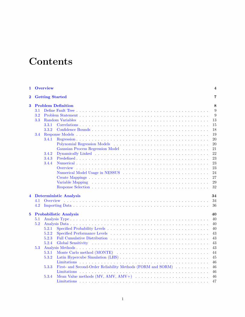
The NESSUS GUI employs the traditional document data paradigm, whereby one or more NESSUS“documents” may be created, opened, and modified. The contents of the analysis are summarized by adisplayed outline, which changes as the analysis is developed. The outline (Figure 1.1) guides you throughthe steps of developing an analysis, ending with the initiation of a NESSUS job run and the visualization ofthe computed results.
You navigate through the contents of the analysis by selecting the nodes of the outline. The area tothe right of the outline changes depending on which outline node is selected. Although the outline helpsguide you through the analysis development in a linear fashion, you have the freedom to navigate throughthe outline in any order you wish. However, certain portions of the outline do not appear until the datarequired for them to appear has been entered.
It is important to note that an analysis is developed in a top down approach, starting with defining aproblem statement and random variables, followed by model definitions, analysis type selection, analysisexecution, and ending with results visualization. Once an analysis has been defined, you can go back andmodify inputs as needed and re-perform the analysis.
A powerful feature of NESSUS is ability to link models together in a sequential fashion. In the problemstatement window, each model is defined only in terms of input and output. This improves readability,conveys the essential flow of the analysis, and allows complex reliability assessments to be defined whenmore than one model is required, for example, a stress computed from a finite element model can be passedinto an analytical equation that computes fatigue life. In the example shown here, a response model (σmax =SigmaMax) is linked to a failure model (g = Paris crack growth law), i.e.,
g =2(a1−n/2f − a1−n/2i
)1.16× 10⁻⁹(2− n) (Y σmax
√n)
n
σmax =3PS
2B2
or in Fortran syntax,
g=2*(af**(1-n/2)-ai**(1-n/2))/(1.16E-9*(2-n)*(Y*SigmaMax*sqrt(Pi))**n)
SigmaMax=3*P*S/2/B**2
The multiple model capability is also useful for breaking a complex model into smaller more manageableparts. For example, a complicated analytical response model can be defined using two or more expressions,which when executed in sequence, results in the original analytical response model.
4
Figure 1.1: NESSUS outline
5

You may save and restore an analysis at any point in its development. The complete state of the analysisis saved in the “jobname.dat” file, which can be read using any text editor.
6

Chapter 2
Getting Started
After the GUI has been started, you must either create a new analysis file, or open an existing one. Thiscan be done via one of the first two buttons of the tool bar, or from the File menu.
The outline (Figure 1.1 will appear after starting new or resuming from a previously saved session. Theoutline is intended to logically guide the user through the problem setup, analysis and visualization of results.
7
Chapter 3
Problem Definition
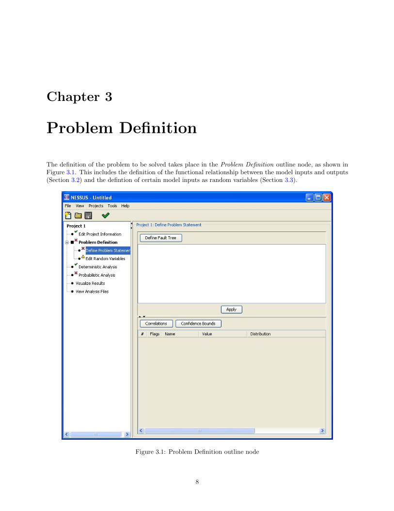
The definition of the problem to be solved takes place in the Problem Definition outline node, as shown inFigure 3.1. This includes the definition of the functional relationship between the model inputs and outputs(Section 3.2) and the defintion of certain model inputs as random variables (Section 3.3).
Figure 3.1: Problem Definition outline node
8
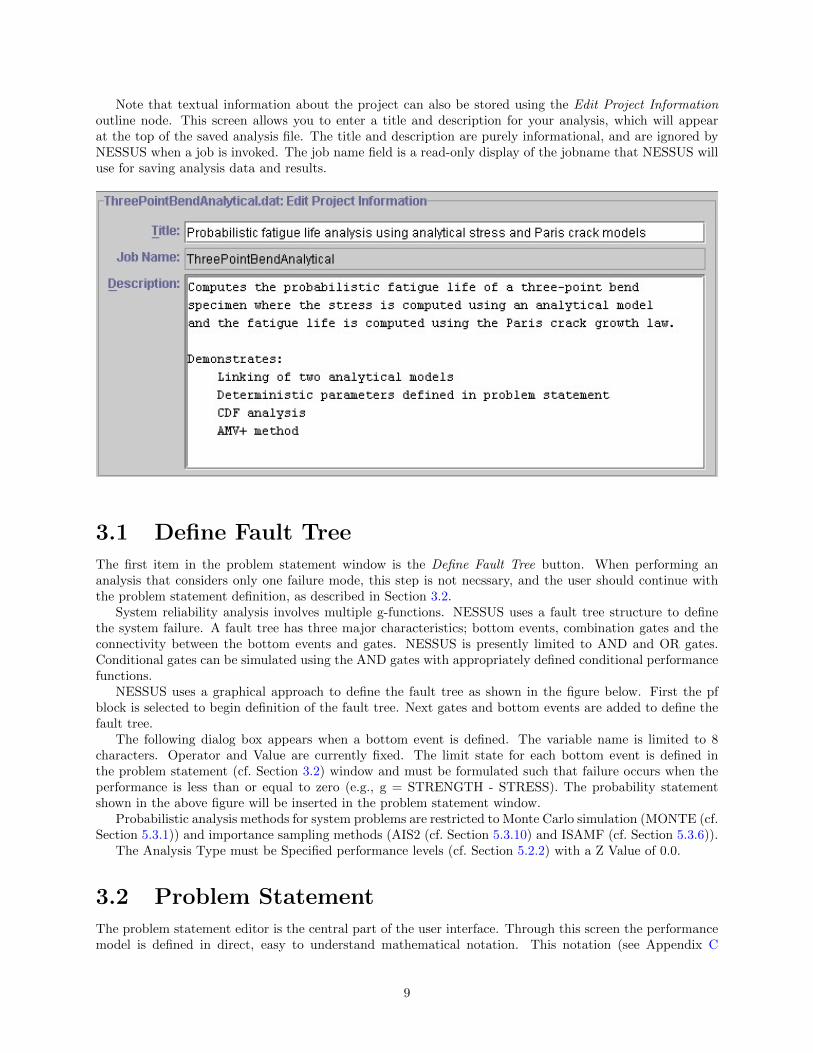
Note that textual information about the project can also be stored using the Edit Project Informationoutline node. This screen allows you to enter a title and description for your analysis, which will appearat the top of the saved analysis file. The title and description are purely informational, and are ignored byNESSUS when a job is invoked. The job name field is a read-only display of the jobname that NESSUS willuse for saving analysis data and results.
3.1 Define Fault Tree
The first item in the problem statement window is the Define Fault Tree button. When performing ananalysis that considers only one failure mode, this step is not necssary, and the user should continue withthe problem statement definition, as described in Section 3.2.
System reliability analysis involves multiple g-functions. NESSUS uses a fault tree structure to definethe system failure. A fault tree has three major characteristics; bottom events, combination gates and theconnectivity between the bottom events and gates. NESSUS is presently limited to AND and OR gates.Conditional gates can be simulated using the AND gates with appropriately defined conditional performancefunctions.
NESSUS uses a graphical approach to define the fault tree as shown in the figure below. First the pfblock is selected to begin definition of the fault tree. Next gates and bottom events are added to define thefault tree.
The following dialog box appears when a bottom event is defined. The variable name is limited to 8characters. Operator and Value are currently fixed. The limit state for each bottom event is defined inthe problem statement (cf. Section 3.2) window and must be formulated such that failure occurs when theperformance is less than or equal to zero (e.g., g = STRENGTH - STRESS). The probability statementshown in the above figure will be inserted in the problem statement window.
Probabilistic analysis methods for system problems are restricted to Monte Carlo simulation (MONTE (cf.Section 5.3.1)) and importance sampling methods (AIS2 (cf. Section 5.3.10) and ISAMF (cf. Section 5.3.6)).
The Analysis Type must be Specified performance levels (cf. Section 5.2.2) with a Z Value of 0.0.
3.2 Problem Statement
The problem statement editor is the central part of the user interface. Through this screen the performancemodel is defined in direct, easy to understand mathematical notation. This notation (see Appendix C
9

Figure 3.2: Probabilistic Fault Tree Definition in NESSUS
10
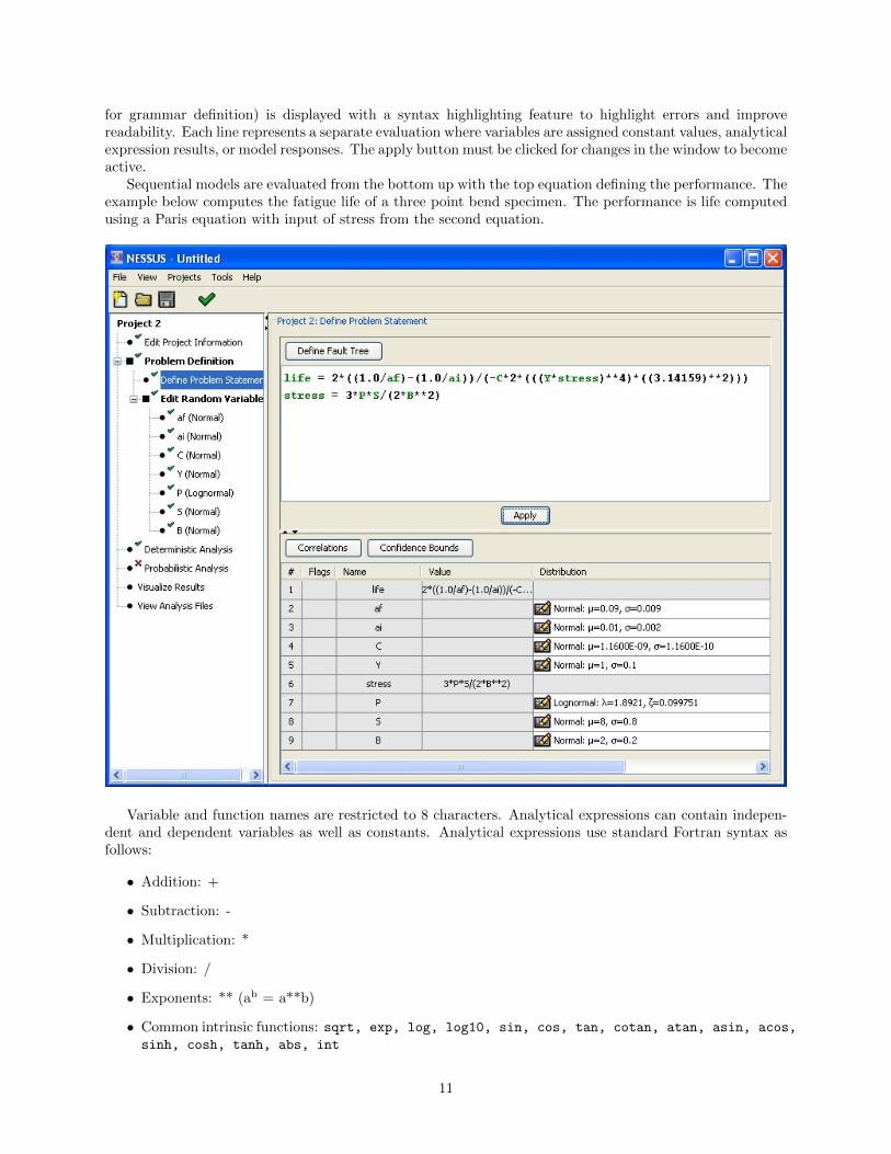
for grammar definition) is displayed with a syntax highlighting feature to highlight errors and improvereadability. Each line represents a separate evaluation where variables are assigned constant values, analyticalexpression results, or model responses. The apply button must be clicked for changes in the window to becomeactive.
Sequential models are evaluated from the bottom up with the top equation defining the performance. Theexample below computes the fatigue life of a three point bend specimen. The performance is life computedusing a Paris equation with input of stress from the second equation.
Variable and function names are restricted to 8 characters. Analytical expressions can contain indepen-dent and dependent variables as well as constants. Analytical expressions use standard Fortran syntax asfollows:
• Addition: +
• Subtraction: -
• Multiplication: *
• Division: /
• Exponents: ** (ab = a**b)
• Common intrinsic functions: sqrt, exp, log, log10, sin, cos, tan, cotan, atan, asin, acos,
sinh, cosh, tanh, abs, int
11

• The argument for trigonometric intrinsic functions use radians
Syntax highlighting is as follows:
• blue – functions
• green – variables
• black – operators, groupings, and numbers
• orange – intrinsics
• red – error (typically more than 8 characters for a variable or function name, non matching parentheses,equation error)
Response models are declared as functions as shown in the following example. This example computesthe fatigue life of a three point bend specimen. The equations are evaluated from the bottom up with thefinal performance defined by the life variable. This example uses the stress computed from the “fe” functionas input to the Paris equation. The “fe” function is defined in the “Define Response Models” section of theoutline in the GUI. See the Response Models (cf. Section 3.4) section for information on how to define theresponse model.
When defining functions the form of the equation cannot contain any mathematical operators or intrinsicfunctions. Note that parameters can also be included in the problem statement by equating the variable toa value.
Multiple response variables can be equated to a function using the format in the following figure. Eachof these response variables will be defined in the "Define Response Models" section in the GUI.
The GUI differentiates between dependent variables and independent random variables. After a problemstatement is entered or modified, and the Apply button is clicked, the GUI parses the equation and determineswhether a variable is dependent or independent. Although default inputs are provided, independent variablesmust be defined by specifying a distribution, mean and standard deviation. Variables can be changed fromindependent to dependent and back by changing the problem statement definition.
Below the problem statement editor is a table displaying the variables detected when the Apply buttonis pressed. The inputs for the independent variables can be edited in this table. A detailed description ofthis table can be found in the Random Variables (cf. Section 3.3) section.
Reminders for defining the problem statement:
12
• Equations are evaluated from the bottom up
• Variable and function names are limited to 8 characters
• Press the "Apply" button to apply changes
3.3 Random Variables
After a problem statement is entered and applied, the GUI processes all variables to determine whetherthey are dependent variables or independent random variables. Random variables are assigned a defaultdistribution that can then be edited in several ways.
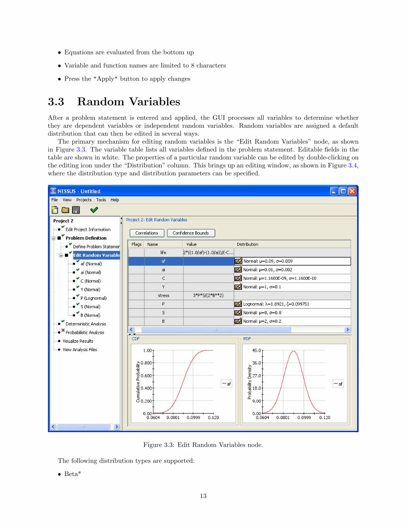
The primary mechanism for editing random variables is the “Edit Random Variables” node, as shownin Figure 3.3. The variable table lists all variables defined in the problem statement. Editable fields in thetable are shown in white. The properties of a particular random variable can be edited by double-clicking onthe editing icon under the “Distribution” column. This brings up an editing window, as shown in Figure 3.4,where the distribution type and distribution parameters can be specified.
Figure 3.3: Edit Random Variables node.
The following distribution types are supported:
• Beta*
13
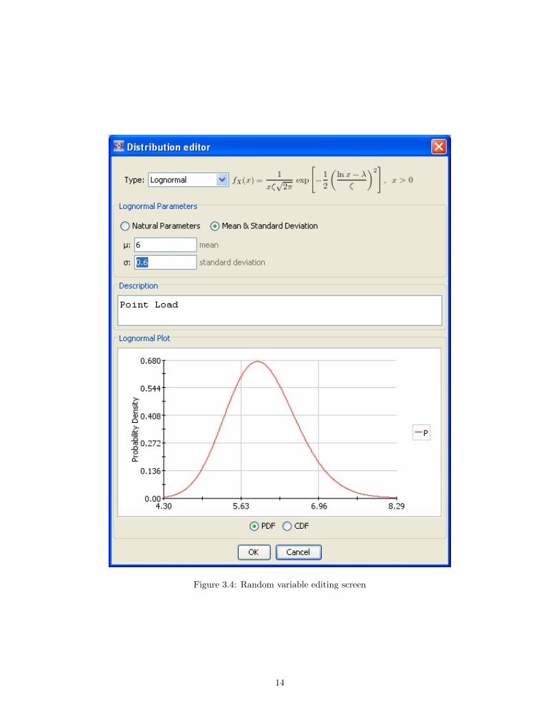
Figure 3.4: Random variable editing screen
14

• Chi-square
• Exponential*
• Frechet*
• GEVDmax (Generalized Extreme Value for maxima)*
• GEVDmin (Generalized Extreme Value for minima)*
• Gamma*
• Gumbel
• Lognormal
• Normal
• Pareto*
• Triangular*
• Truncated Normal
• Truncated Weibull
• Uniform
• Weibull
The starred distributions are only supported by following probabilistic analysis methods (see Section 5.3):MONTE, LHS, ISMPP, EGRA, and RSM GP.
The parameters governing most random variables can be specified using one of two schemes: “Naturalparameters” or “Moments.” All random variables can be specified using some distribtuion-specific set ofnatrual parameters. For example, the natural parameters of the uniform distribution are the lower and upperbounds. Most random variables can also be specified by the “Moments,” which are the mean and standarddeviation.1 Where applicable, the radio buttons allow the user to switch between the two schemes.
As seen in Figure 3.3, selecting a random variable in the table will create plots of both the PDF (Probabil-ity Density Function) and CDF (Cumulative Density Function) for that random variable. Multiple randomvariables can be displayed by selecting a range of variables in the table using the shift key along with theleft mouse button or individually using the crtl key with the left mouse button, as shown in Figure 3.5.
There are two additional ways of editing the random variables. First, the Define Problem Statementnode provides a variable table that allows editing, similar to the one from the Edit Random Variables node.Second, a dedicated node is created in the outline for each random variable, as a sub-item of the Edit RandomVariables node (see Figure 3.3). Selecting the node for a particular random variable brings up a screen thatworks in the same way as the the popup window shown in Figure 3.4.
3.3.1 Correlations
The random variable correlation editor is accessed by clicking the Correlations button on either the DefineProblem Statement or Edit Random Variable nodes. Random variable correlations are defined by filling invalues in the lower left triangle of the correlation matrix. By definition, the matrix is symmetric with valuesof 1.0 on the diagonal; these values are shown for reference only and cannot be changed. The off-diagonalcorrelations are restricted to the range of -1.0 to 1.0.
A symbol in the Flags column of the random variables table is used to flag each variable that has anonzero correlation with another variable, as seen in Figure 3.6. This feature provides the user a quickindication of whether correlations have been set, and for which random variables.
The transformations used for correlated variables in NESSUS currently only support the following dis-tributions:
1For the truncated normal and truncated weibull distributions, the mean and standard deviation should be the values beforethe truncation.
15
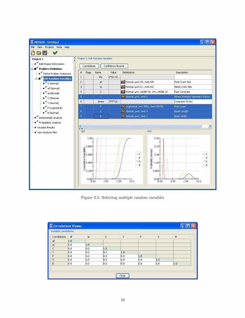
Figure 3.5: Selecting multiple random variables
16
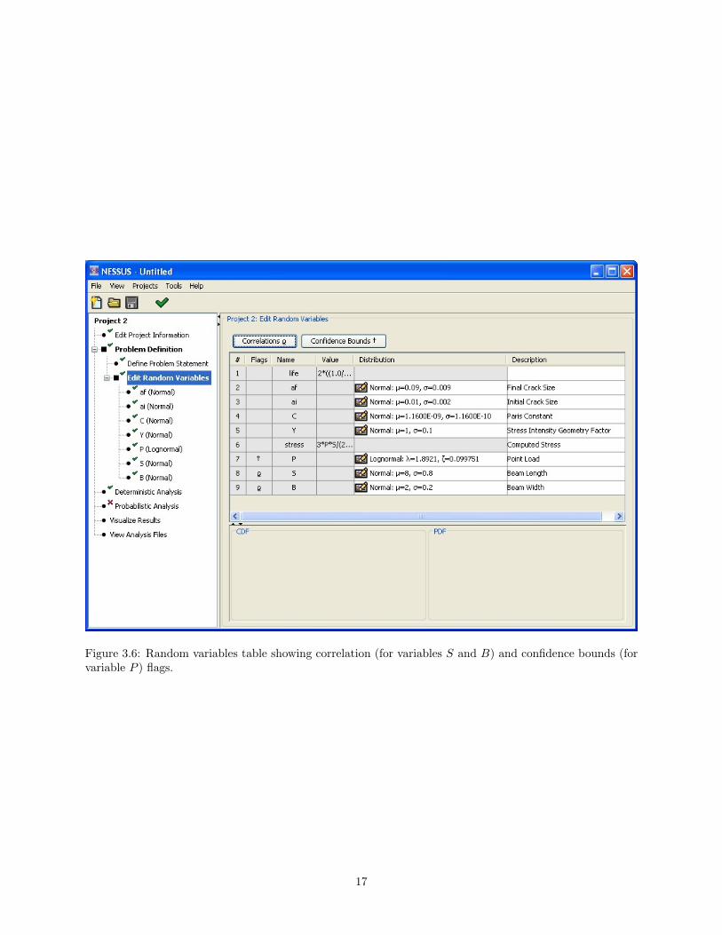
Figure 3.6: Random variables table showing correlation (for variables S and B) and confidence bounds (forvariable P ) flags.
17

• Weibull
• Normal
• Gumbel
• Lognormal
• Frechet
Please contact SwRI if an analysis requires an unsupported distribution for correlated variables and aprerelease may be available.
3.3.2 Confidence Bounds
Each random variable in the problem statement may have some amount of statistical uncertainty assignedto it. The cumulative effect of these statistical uncertainties gives rise to confidence bounds on the computedcumulative distribution function.
The Confidence Bounds editor can be accessed by clicking the Confidence Bounds button on either theDefine Problem Statement or Edit Random Variables nodes. The Confidence Bounds editor allows the userto specify the mean coefficient of variation (COV) and standard deviation COV for each random variable,as seen in Figure 3.7. A distribution type of either uniform or normal may be used for the mean, while thedistribution type for the standard deviation is assumed to be lognormal and cannot be changed.
Figure 3.7: Set confidence bounds
The following settings are also available:
18
• Number of samples: Number of Monte Carlo samples used to compute the confidence bounds. Mustbe greater or equal to 1,000 and less than or equal to 10,000.
• Starting seed: Initial seed for random number generation
• Calculation method: Exact indicates that the true g-function is used to compute the confidencebounds, while Linear approximation uses a first-order approximation during the confidence boundcalculation. Depending on the complexity of the problem being solved, the use of a first-order approx-imation can result in a significant time savings.
Finally, the confidence bounds can computed at up to five confidence levels specified under Bounds Levels.The default is to compute the confidence bounds at the 95% and 90% levels.
As with correlations, a symbol is inserted into the Flags column of the random variable table to indicatewhen confidence bounds have been set for a particular variable. This is seen in Figure 3.6, which shows aconfidence bounds flag for the variable P .
3.4 Response Models
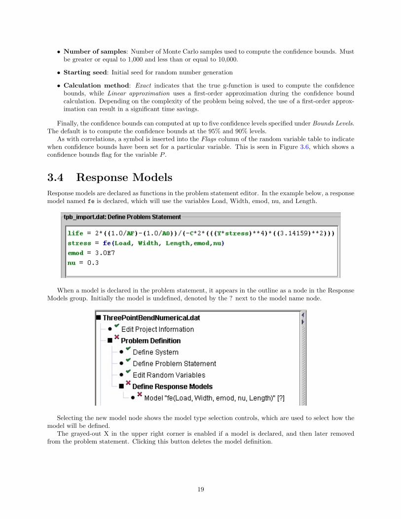
Response models are declared as functions in the problem statement editor. In the example below, a responsemodel named fe is declared, which will use the variables Load, Width, emod, nu, and Length.
When a model is declared in the problem statement, it appears in the outline as a node in the ResponseModels group. Initially the model is undefined, denoted by the ? next to the model name node.
Selecting the new model node shows the model type selection controls, which are used to select how themodel will be defined.
The grayed-out X in the upper right corner is enabled if a model is declared, and then later removedfrom the problem statement. Clicking this button deletes the model definition.
19

3.4.1 Regression
Functions defined in the problem statement window can be defined using a regression model. There are twotypes of regression models available: polynomials (linear, incomplete quadratic, and quadratic) and Gaussianprocess.
Polynomial Regression Models
The polynomial regression models can be defined by either perturbation data or by polynomial coefficients.Perturbation data can be entered in manually or can be imported in from comma delimited file by clickingon the folder icon and selecting the appropriate file Depending on the number of variables and the type ofregression model (Linear, Incomplete Quadratic, or Quadratic) a minimum number of datasets will need tobe given. NESSUS will automatically calculate the minimum number of datasets once the type of regressionmodel has been selected and will be displayed in parentheses.
The equations are given next to the radio buttons where a0 is the constant term, ai are the linear terms,bi are the second order terms, and cij are the cross terms.
z = a0 +
N∑i=1
aiXi +
N∑i=1
biX2i +
N∑i=2
i−1∑j=1
cijXiXj
20

Gaussian Process Regression Model
The Gaussian Process (GP) model (also known as a Kriging model) is a more sophisticaed model basedon spatial correlations. This model can be defined either by providing training data, or by loading a GPmodel file previously created by NESSUS (Figure 3.8). The advantage of loading a saved GP model is thatNESSUS does not have to fit the model, which can be expensive, particularly with larger data sets.
Whenever NESSUS fits a Gaussian Process model, it will save the results to a file, which can then bere-used as a regression model in NESSUS without the need to re-fit the model. Currently, NESSUS willautomatically save GP models in the following cases:
1. A GP regression model is defined in terms of regression data. In this case, the saved model will havethe filename [model].rsm, where [model] is the user-defined response model name.
2. A GP regression model is created as part of either the RSM_GP or EGRA probabilistic methods. In thesecases, the model is saved to the file [analysis].rsm, where [analysis] is the NESSUS project name.
The GP model files created in each of these cases can then be re-used by defining a new GP regression modeland using the “Saved GP model” option. As mentioned above, this avoids the need to re-fit the model eachtime NESSUS is run, which can drastically reduce the run time when working with large data sets.
When defining a GP model in terms of regression data, the user may also specify the level of “noise” orrandom error associated with the observed response values. The options are “None”, “Estimate” (NESSUSwill identify the best-fitting noise level), or “User-specified value”. If provided, the user-specified valuerepresents the standard deviation (or standard error) associated with the random noise. If the data comefrom a deterministic process, such as a computer simulation, then it often makes sense to use either no noiseor a small value close to zero. When no noise is used, the GP predictions will exactly interpolate all trainingdata. When the noise level is increased, the GP model predictions will smooth or “regress” the training data.When modeling non-deterministic processes, such as physical experiments, it is important to allow for somelevel of noise. In these cases, the recommended approach is to allow NESSUS to automatically determinethe noise level by selecting the “Estimate” option. Estimating the noise level can increase the time requiredto fit the model.
21
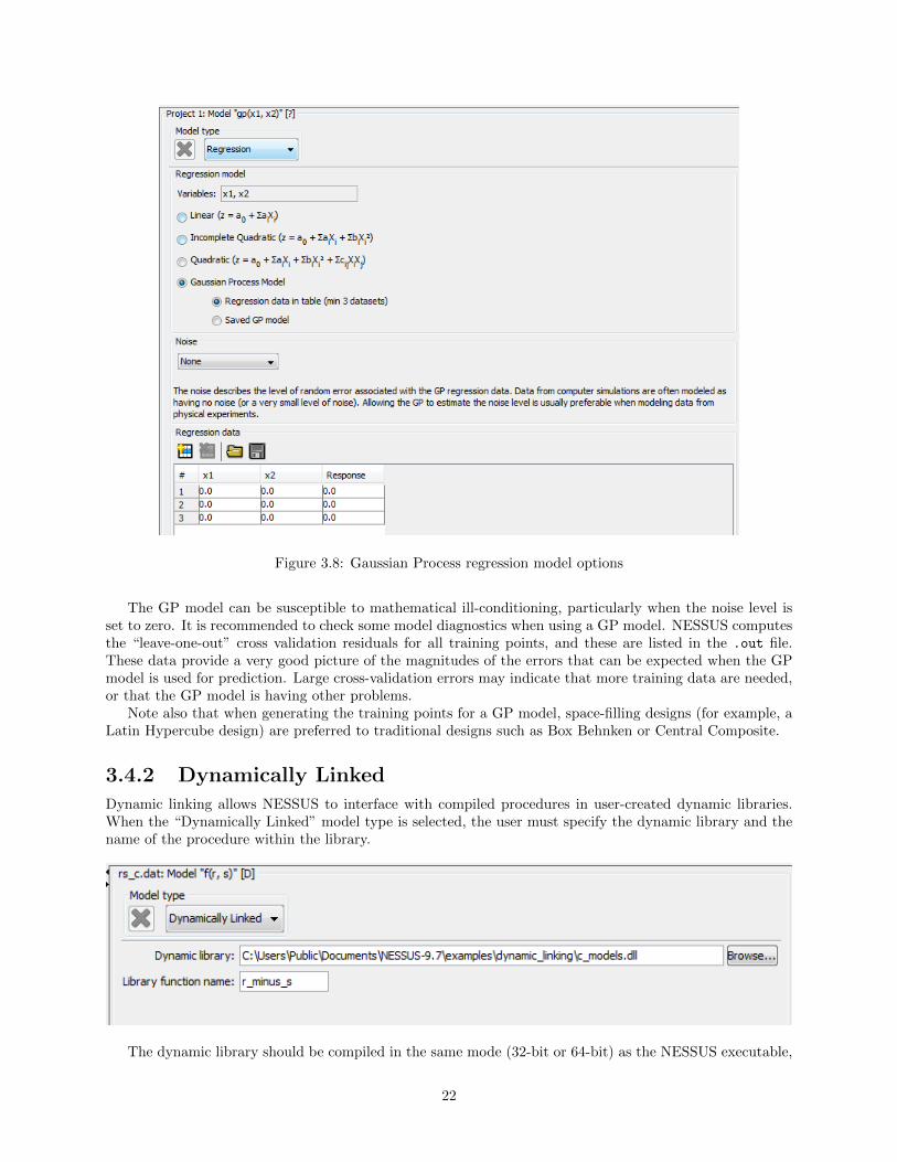
Figure 3.8: Gaussian Process regression model options
The GP model can be susceptible to mathematical ill-conditioning, particularly when the noise level isset to zero. It is recommended to check some model diagnostics when using a GP model. NESSUS computesthe “leave-one-out” cross validation residuals for all training points, and these are listed in the .out file.These data provide a very good picture of the magnitudes of the errors that can be expected when the GPmodel is used for prediction. Large cross-validation errors may indicate that more training data are needed,or that the GP model is having other problems.
Note also that when generating the training points for a GP model, space-filling designs (for example, aLatin Hypercube design) are preferred to traditional designs such as Box Behnken or Central Composite.
3.4.2 Dynamically Linked
Dynamic linking allows NESSUS to interface with compiled procedures in user-created dynamic libraries.When the “Dynamically Linked” model type is selected, the user must specify the dynamic library and thename of the procedure within the library.
The dynamic library should be compiled in the same mode (32-bit or 64-bit) as the NESSUS executable,
22
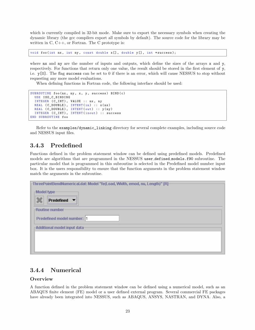
which is currently compiled in 32-bit mode. Make sure to export the necessary symbols when creating thedynamic library (the gcc compilers export all symbols by default). The source code for the library may bewritten in C, C++, or Fortran. The C prototype is:
void foo(int nx, int ny, const double x[], double y[], int *success );
where nx and ny are the number of inputs and outputs, which define the sizes of the arrays x and y,respectively. For functions that return only one value, the result should be stored in the first element of y,i.e. y[0]. The flag success can be set to 0 if there is an error, which will cause NESSUS to stop withoutrequesting any more model evaluations.
When defining functions in Fortran code, the following interface should be used:
SUBROUTINE foo(nx, ny , x, y, success) BIND(c)
USE ISO_C_BINDING
INTEGER (C_INT), VALUE :: nx, ny
REAL (C_DOUBLE), INTENT(in) :: x(nx)
REAL (C_DOUBLE), INTENT(out) :: y(ny)
INTEGER (C_INT), INTENT(inout) :: success
END SUBROUTINE foo
Refer to the examples/dynamic_linking directory for several complete examples, including source codeand NESSUS input files.
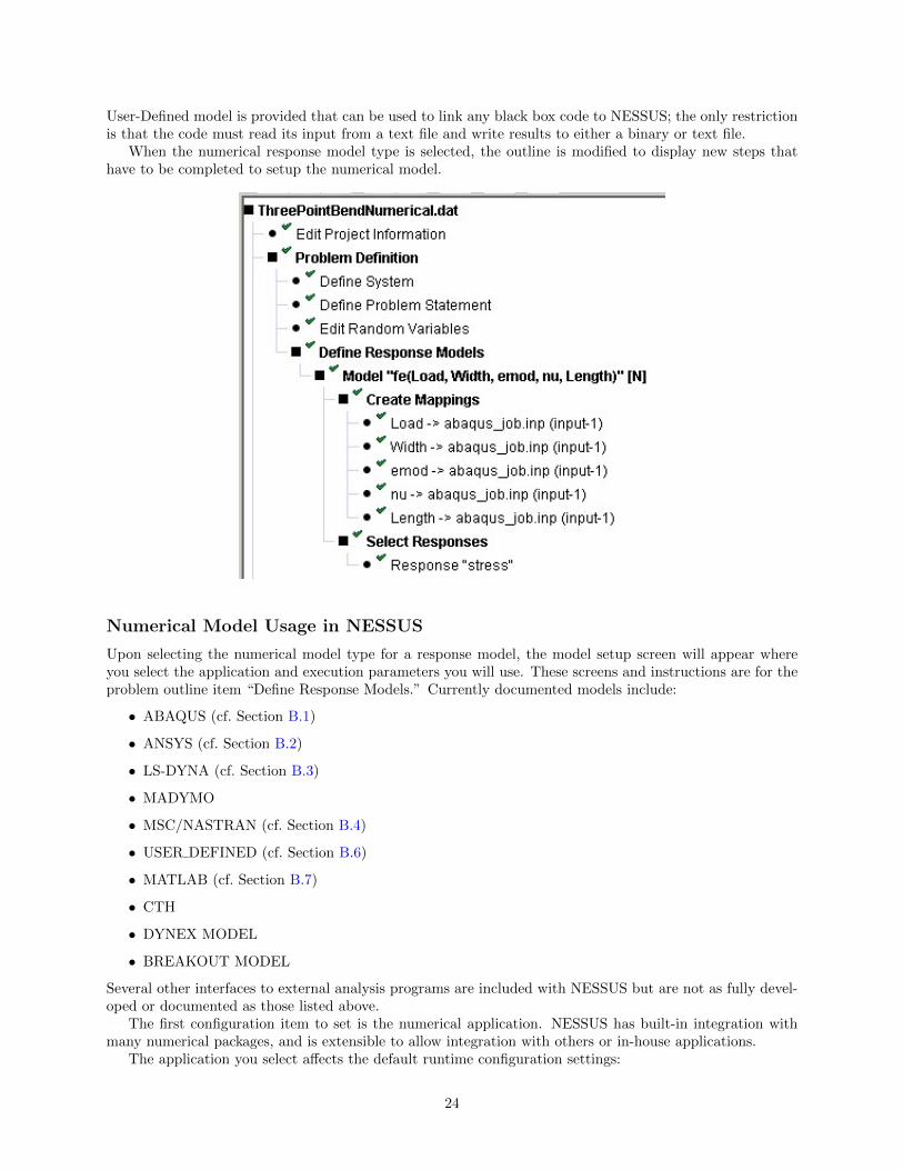
3.4.3 Predefined
Functions defined in the problem statement window can be defined using predefined models. Predefinedmodels are algorithms that are programmed in the NESSUS user defined models.f90 subroutine. Theparticular model that is programmed in this subroutine is selected in the Predefined model number inputbox. It is the users responsibility to ensure that the function arguments in the problem statement windowmatch the arguments in the subroutine.
3.4.4 Numerical
Overview
A function defined in the problem statement window can be defined using a numerical model, such as anABAQUS finite element (FE) model or a user defined external program. Several commercial FE packageshave already been integrated into NESSUS, such as ABAQUS, ANSYS, NASTRAN, and DYNA. Also, a
23
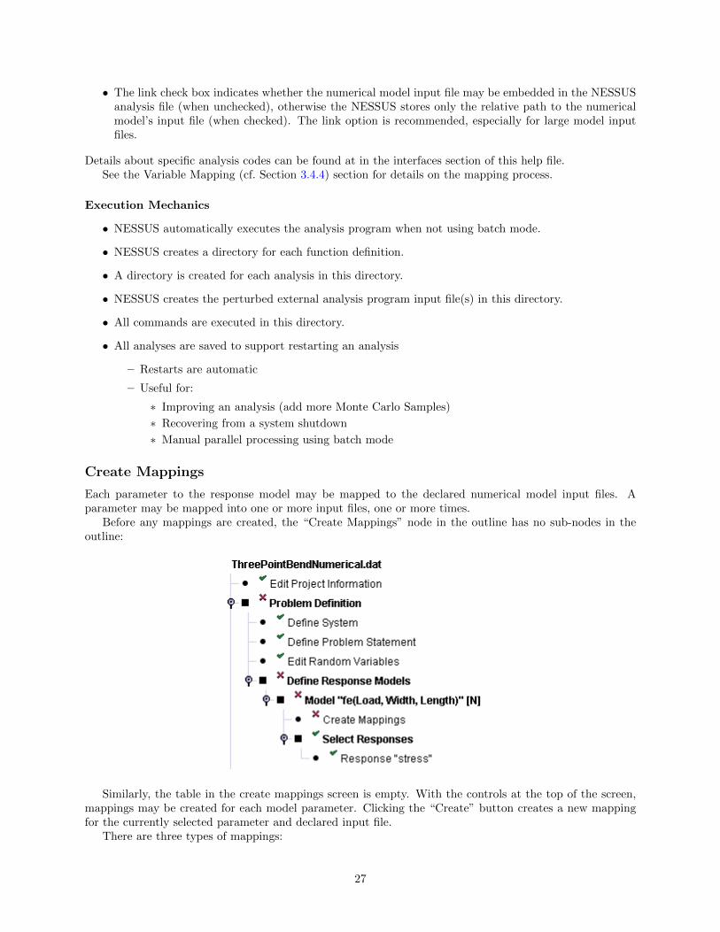
User-Defined model is provided that can be used to link any black box code to NESSUS; the only restrictionis that the code must read its input from a text file and write results to either a binary or text file.
When the numerical response model type is selected, the outline is modified to display new steps thathave to be completed to setup the numerical model.
Numerical Model Usage in NESSUS
Upon selecting the numerical model type for a response model, the model setup screen will appear whereyou select the application and execution parameters you will use. These screens and instructions are for theproblem outline item “Define Response Models.” Currently documented models include:
• ABAQUS (cf. Section B.1)
• ANSYS (cf. Section B.2)
• LS-DYNA (cf. Section B.3)
• MADYMO
• MSC/NASTRAN (cf. Section B.4)
• USER DEFINED (cf. Section B.6)
• MATLAB (cf. Section B.7)
• CTH
• DYNEX MODEL
• BREAKOUT MODEL
Several other interfaces to external analysis programs are included with NESSUS but are not as fully devel-oped or documented as those listed above.
The first configuration item to set is the numerical application. NESSUS has built-in integration withmany numerical packages, and is extensible to allow integration with others or in-house applications.
The application you select affects the default runtime configuration settings:
24

25

• Execution command
• Input files
• Output files
The parameters available in the response selection screen are also affected (see Response Selection (cf.Section 3.4.4) section).
If the default execution command does not reflect the solver setup on your platform it may be changedon the execution command screen. The execution command is saved in the NESSUS input file.
Once the application is selected default input and output files are declared. If supported by the applica-tion, the number of input and output files may be changed with the add and delete buttons.
The input files are the files that NESSUS will modify with probabilistic values and pass to the numericalpackage for solution. The output files are the files that NESSUS expects to parse for obtaining responses.At a minimum, the path to the numerical application’s input files must be specified. In the example belowone input file and one output file have been declared.
• The path to the source file needs to be specified by either typing in the path or clicking the ellipses tobring up a file browser dialog.
• The destination name specifies the file name that NESSUS will create to store the input file after ithas been modified with the variable mappings. This destination file name must be consistent with theexecution command.
• The label is a unique identifier used by NESSUS to track variable mappings. The value of the labelmust be unique across all input files for the current model. The default value should be sufficient inmost cases.
26
• The link check box indicates whether the numerical model input file may be embedded in the NESSUSanalysis file (when unchecked), otherwise the NESSUS stores only the relative path to the numericalmodel’s input file (when checked). The link option is recommended, especially for large model inputfiles.
Details about specific analysis codes can be found at in the interfaces section of this help file.See the Variable Mapping (cf. Section 3.4.4) section for details on the mapping process.
Execution Mechanics
• NESSUS automatically executes the analysis program when not using batch mode.
• NESSUS creates a directory for each function definition.
• A directory is created for each analysis in this directory.
• NESSUS creates the perturbed external analysis program input file(s) in this directory.
• All commands are executed in this directory.
• All analyses are saved to support restarting an analysis
– Restarts are automatic
– Useful for:
∗ Improving an analysis (add more Monte Carlo Samples)
∗ Recovering from a system shutdown
∗ Manual parallel processing using batch mode
Create Mappings
Each parameter to the response model may be mapped to the declared numerical model input files. Aparameter may be mapped into one or more input files, one or more times.
Before any mappings are created, the “Create Mappings” node in the outline has no sub-nodes in theoutline:
Similarly, the table in the create mappings screen is empty. With the controls at the top of the screen,mappings may be created for each model parameter. Clicking the “Create” button creates a new mappingfor the currently selected parameter and declared input file.
There are three types of mappings:
27

Replace: The parameter is mapped into a well-formatted text-based input file with line and column defini-tion sets. This mapping directly replaces the parameter value in the input file. This mapping cannotoverlap with any other mapping.
Vector Scaling: The parameter is mapped into a well-formatted text-based input file with line and columndefinition sets and datablocks. See the Variable Mapping (cf. Section 3.4.4) description for details.
Automatic: NESSUS applies the mapping internally through specialized coding for a given numericalmodel and response type. For example, a history file consisting of time and acceleration can bedefined for an LS-DYNA model. This history file can then be used as input to a subsequent model.Automatic mappings are currently supported for all LS-DYNA response quantities, NASA-GRC-HTMtemperature results, and all DYNA2D and DYNA3D response quantities.
The image below shows a complete set of created mappings for the model
fe(Load, Width, emod, nu, Length)
whereby all parameters are mapped into the input file abaqus job.inp.
28
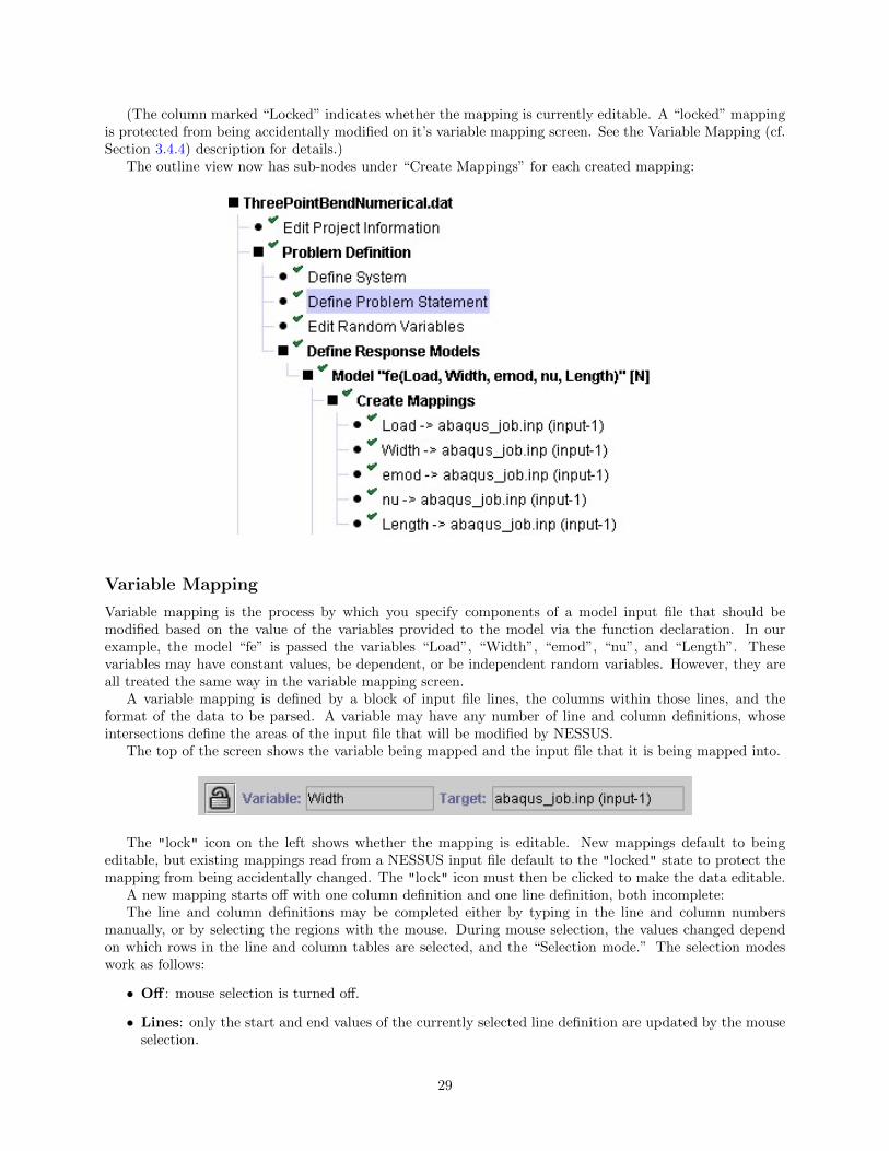
(The column marked “Locked” indicates whether the mapping is currently editable. A “locked” mappingis protected from being accidentally modified on it’s variable mapping screen. See the Variable Mapping (cf.Section 3.4.4) description for details.)
The outline view now has sub-nodes under “Create Mappings” for each created mapping:
Variable Mapping
Variable mapping is the process by which you specify components of a model input file that should bemodified based on the value of the variables provided to the model via the function declaration. In ourexample, the model “fe” is passed the variables “Load”, “Width”, “emod”, “nu”, and “Length”. Thesevariables may have constant values, be dependent, or be independent random variables. However, they areall treated the same way in the variable mapping screen.
A variable mapping is defined by a block of input file lines, the columns within those lines, and theformat of the data to be parsed. A variable may have any number of line and column definitions, whoseintersections define the areas of the input file that will be modified by NESSUS.
The top of the screen shows the variable being mapped and the input file that it is being mapped into.
The "lock" icon on the left shows whether the mapping is editable. New mappings default to beingeditable, but existing mappings read from a NESSUS input file default to the "locked" state to protect themapping from being accidentally changed. The "lock" icon must then be clicked to make the data editable.
A new mapping starts off with one column definition and one line definition, both incomplete:The line and column definitions may be completed either by typing in the line and column numbers
manually, or by selecting the regions with the mouse. During mouse selection, the values changed dependon which rows in the line and column tables are selected, and the “Selection mode.” The selection modeswork as follows:
• Off : mouse selection is turned off.
• Lines: only the start and end values of the currently selected line definition are updated by the mouseselection.
29

30

• Columns: only the start and end values of the currently selected column definition are updated bythe mouse selection.
• Both: the start and end values of both the currently selected line and column definitions are updatedby the mouse selection.
After the mouse selection is performed, the selection color and selection region is updated to reflect theselected line and column definitions. The image below shows the region defined by the first line and columndefinitions.
The format cell in the column definition is used to tell NESSUS how to write the numbers in the definedregion. The cell value follows standard FORTRAN syntax for formatting numbers. For example:
• Scientific format with six decimal places and width of 13 characters: E13.6
• Floating point format: F10.6
As seen in the image below, when the format field is being edited an ellipses button appears. Doubleclick in the format box to allow editing.
Clicking this button displays a dialog aiding in the format definition for users not familiar with theFORTRAN formatting syntax:
Once the mapping is defined, a delta vector is necessary to tell NESSUS how changes in variable changesmultiple quantities in the defined region. A delta vector may be specified one of three ways via the associationselection, defined as follows:
31
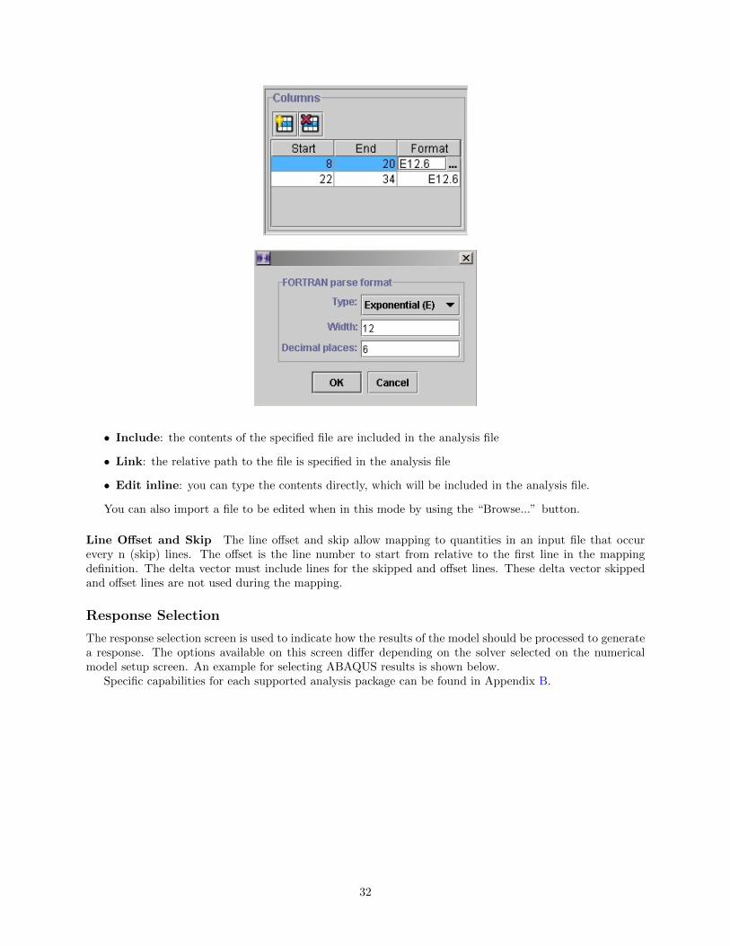
• Include: the contents of the specified file are included in the analysis file
• Link: the relative path to the file is specified in the analysis file
• Edit inline: you can type the contents directly, which will be included in the analysis file.
You can also import a file to be edited when in this mode by using the “Browse...” button.
Line Offset and Skip The line offset and skip allow mapping to quantities in an input file that occurevery n (skip) lines. The offset is the line number to start from relative to the first line in the mappingdefinition. The delta vector must include lines for the skipped and offset lines. These delta vector skippedand offset lines are not used during the mapping.
Response Selection
The response selection screen is used to indicate how the results of the model should be processed to generatea response. The options available on this screen differ depending on the solver selected on the numericalmodel setup screen. An example for selecting ABAQUS results is shown below.
Specific capabilities for each supported analysis package can be found in Appendix B.
32

33
Chapter 4
Deterministic Analysis
4.1 Overview
Before proceeding with a probabilistic analysis, it is recommended that the user verify that their model isset up correctly in NESSUS. This is particularly important when interfacing with numerical models, in orderto verify that the variable mapping has been set up correctly. NESSUS provides the capability to verify theperformance model using the Deterministic Analysis node, which allows the user to run the model usingspecified input values and confirm that the outputs are as expected.
In the development of an analysis it is also useful to gain insight into the sensitivity and behavior of thevariables in use. The Deterministic Analysis node provides the functionality for carrying out these types ofstudies.
Upon selecting the Deterministic Analysis node, the window will look something like the one in Figure 4.1.The Deterministic Input Values section shows a table listing of parameter values that are set to be run. Eachrow of the table corresponds to a set of input values to run, and each random variable has a column whereit’s input may be specified.
In Figure 4.1, the problem contains two random variables: r and s. NESSUS will always initialize thetable with Row #0, which corresponds to the mean value run: the mean is used for each random variable(in this case, the mean of r is 1000 and the mean of s is 800). The mean value run is required by NESSUS,so the user may not remove or edit this row.
The user may add additional rows to the table either one-at-a-time or as a group by specifying a designof experiments or parameter variation scheme. To add a single new row, click on the second icon from theleft. The row comes initialized with blank cells: any cell left blank means that that the mean value will beused for that input. The user may edit the value of any cell simply by clicking on the cell, typing a newvalue, and hitting enter. The units for values entered in this manner are determined using the “Editingmode” drop down selection, which specifies either natural or standard normal units. Cells that are specifiedin standard normal units are identified in the table by a “u” symbol.
NESSUS also provides the capability to generate multiple deterministic input values, which simplifies theprocess of creating a design of experiments or sensitivity study. To generate multiple input values, click onthe “gear” icon, which is the one at the far left. This brings up a dialog like Figure 4.2.
The supported methods for generating deterministic input values are:
• Box Behnken
• Central Composite
• Forward Difference
• Backward Difference
• Central Difference
• Problem Variable Ranges
34

Figure 4.1: Deterministic Analysis window showing initial “Mean value” run
35

Figure 4.2: Dialog for generating deterministic input values
• Two Level Full Factorial
• Three Level Full Factorial
Depending on the method, the user will either specify a “Delta” (shift from the mean), low/medium/highvalues for a design, or start/end/step values for variation over a range. These values may be specified ineither Standard Normal or Natural units. Figure 4.3 shows the layout of a Central Difference design using aDelta of 0.1 in Standard Normal units. Note that the values are displayed as “0.1 u” in the table, to indicateStandard Normal units.
After the input values are generated, they may be modified or deleted by selecting the cells in the table.Once the input values have been generated, the deterministic analysis can be performed by clicking the
Run button. The user should first select the Response variable of interest: if the problem statement containsmultiple responses, NESSUS will return deterministic results for all responses that feed into the selectedresponse (this way, the user may prevent an expensive numerical model from being run).
The results may be examined by clicking Visualize Results. Note that response plots are only availablefor groups of runs that vary only a single variable. The complete results are stored in the comma delimitedoutput file named <jobname>.dst.
4.2 Importing Data
As of version 9.6, NESSUS provides an enhanced facility for importing external data into the deterministicanalysis table. There are two ways to bring in external data: (1) importing from a file, and (2) pasting fromthe clipboard. In each case, a Table Import Wizard dialog will be brought up, allowing the user to fine tunethe import options and data format before loading the data into the table.
To import data from a file, use the “Open file” icon in the toolbar above the deterministic analysis table.The format of the file may be either comma-separated (CSV) or plain text with whitespace separation orany user-defined other character-delimiter.
To paste data from the clipboard, either press control-V or right-click anywhere on or below the tableand choose Paste.
36
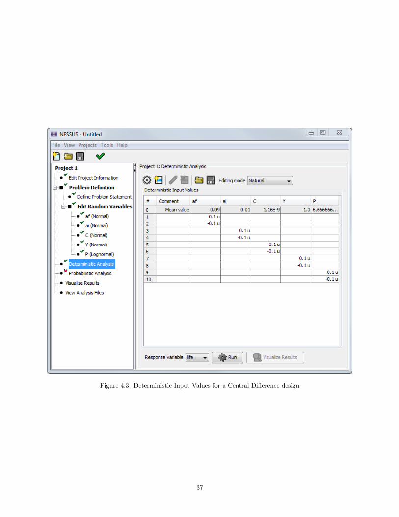
Figure 4.3: Deterministic Input Values for a Central Difference design
37

The Table Import Wizard Dialog, shown in Figure 4.4, will open immediately after selecting a file toimport data from or pasting data from the clipboard. The import wizard provides several options forspecifying how to import the data:
Separator options This section is used to define how the data fields are separated. This may be eitherbased on a fixed number of characters per column (fixed width) or using one or more character de-limiters. When Merge delimiters is selected, multiple consecutive delimiter characters (e.g. multiplespace characters) are treated as a single delimiter. The Skip comment lines option is used to specifycharacters which, when they occur at the beginning of the line, denote lines that should be ignored(i.e. lines that contain “comments”).
Source Start with row specifies the row (i.e. line number) to being importing the source data from. Usinga value greater than one can be used, for example, to skip lines at the top of a file that are used asdata headers.
Destination This section is used to define where the data will be imported into in the NESSUS table.When the table contains existing data, the options Overwrite and Insert can be used to define whetheror not the existing data are overwritten.
Fields The last section of the wizard shows a preview of how the data will be imported into the table. Whenthe source data contain more columns that the NESSUS table, those columns show up in the previewfield in red, labeled “Unbound”. The import operation can not be completed when there are unboundcolumns. This is resolved by “skipping” (i.e. ignoring) selected columns of the source data, which isdone by clicking anywhere in the respective column of the preview pane. Source columns marked tobe skipped are shown in grey.
38
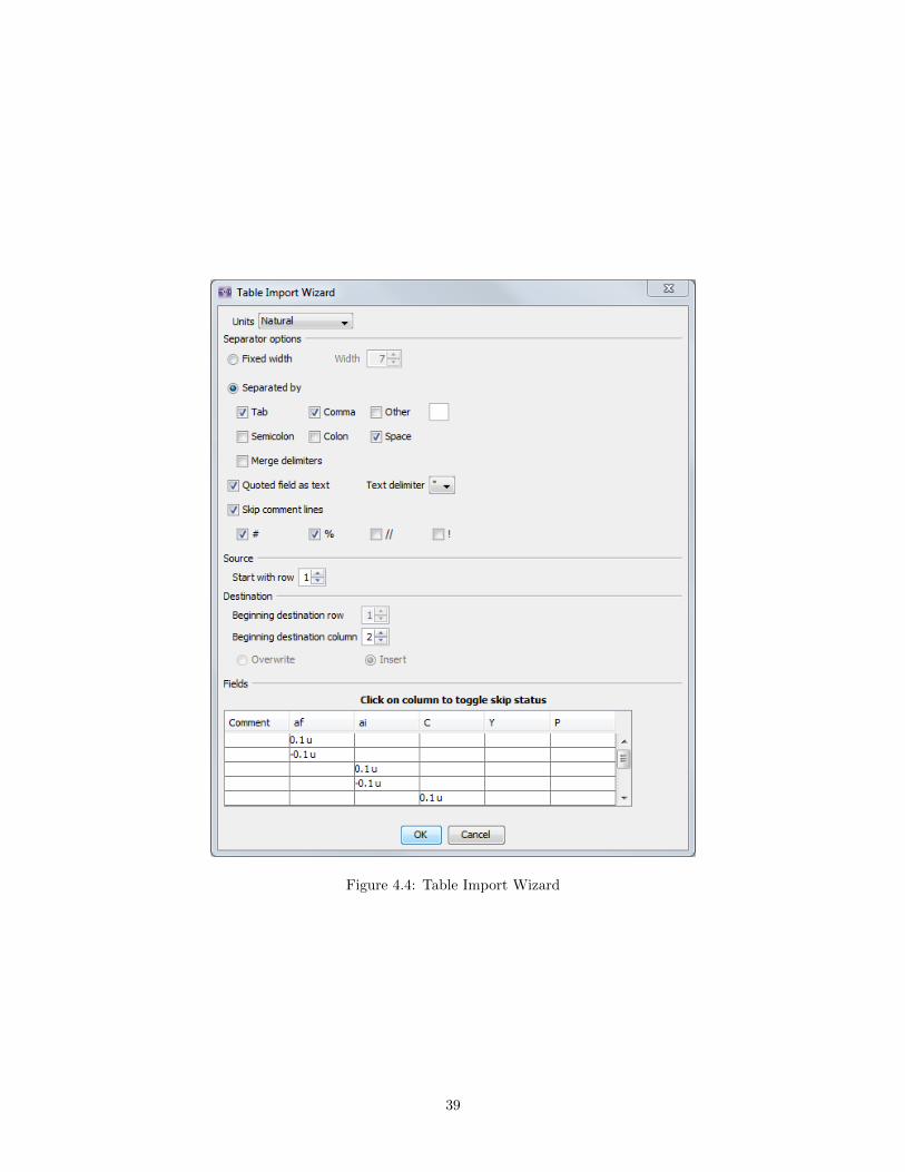
Figure 4.4: Table Import Wizard
39

Chapter 5
Probabilistic Analysis
5.1 Analysis Type
The first time the Probabilistic Analysis node is selected for a particular project, the screen shown inFigure 5.1 is displayed. The user selects the analysis type, but the selection may be changed on the nextscreen. NESSUS categorizes probabilistic analysis into four “analysis types”:
Specified probability levels Sometimes referred to as “inverse reliability analysis,” the user specifies oneor more probabilities, and NESSUS computes the corresponding response levels. Note that for aresponse Z, the probability is interpreted as P [z < Z], where z is a particular response level.
Specified performance levels Sometimes referred to as “forward reliability analysis,” allows the user tospecify one or more performance levels, and NESSUS computes the probability of the response beingless than the specified values.
Full cumulative distribution NESSUS automatically selects and computes multiple probability levels sothat the entire cumulative distribution function of the response can be visualized.
Global sensitivity The sensitivity of the model output is analyzed globally, with respect to model inputprobability distributions.
After making the initial analysis type selection, the Probabilistic Analysis editing window is displayed,as in Figure 5.2. This window is broken into two sections: (1) the top portion is for configuring the analysistype and data, and (2) the bottom portion is for configuring the analysis method.
5.2 Analysis Data
The top portion of the Probabilistic Analysis window (Figure 5.2) allows the user to enter in the analysisdata. The user can also use the drop-down menu in the top-left of the window to change the previouslyselected analysis type. The analysis data to be entered depends on the analysis type.
5.2.1 Specified Probability Levels
The Specified Probability Levels analysis type requires the user to enter probability levels for which NESSUSwill calculate performances. The probability levels may be entered as specific probabilities (0 to 1) or asstandard normal values (-10 to 10). As you enter probability values, the table automatically grows toaccommodate new values. The buttons above the table are for inserting and deleting entries.
40
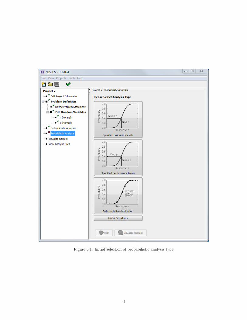
Figure 5.1: Initial selection of probabilistic analysis type
41

Figure 5.2: Probabilistic analysis editing window
42
5.2.2 Specified Performance Levels
The Specified Performance Levels analysis type requires that the user enter specific performance values forwhich NESSUS will compute probabilities. As you enter Z values, the table grows to accommodate newvalues. The buttons above the table are for inserting and deleting entries.
5.2.3 Full Cumulative Distribution
The Full Cumulative Distribution analysis type instructs NESSUS to select approximately 10-12 distributionpoints, selected to span the CDF from approximately 0 to 100%. In this mode, no user-defined analysis dataare needed.
5.2.4 Global Sensitivity
The global sensitivity analysis type does not require any user-defined analysis data.
5.3 Analysis Methods
The bottom portion of the Probabilistic Analysis screen (Figure 5.2), labeled Reliability method, is where theuser configures the probabilistic analysis method that NESSUS will use. NESSUS supports a large numberof probabilistic analysis methods:
• Monte Carlo method (MONTE)
• Latin Hypercube (LHS)
• First order reliability method (FORM)
• Second order reliability method (SORM)
• Mean value (MV)
• Advanced mean value (AMV)
• Advanced mean value with iterations (AMV+)
• Advanced mean value - AIS (AMV AIS)
• Importance sampling w/radius reduction factor (ISAMF)
• Importance sampling w/user-defined radius (ISAMR)
• Importance sampling at user-defined MPP (ISMPP)
• Plane-based adaptive importance sampling (AIS1)
• Curvature-based adaptive importance sampling (AIS2)
• Efficient Global Reliability Analysis (EGRA)
• Response Surface Method (RSM)
• Gaussian Process Response Surface Method (RSM GP)
• Probability Contouring (MV CONT)
• Variance decomposition (VARDCMP)
43
You select the analysis method to use from the drop-down menu at the top of the Reliability Methodediting pane. Some analysis methods require additional parameters and these methods are described insubsequent sections.
Details about the probabilistic algorithms can be found in the NESSUS theoretical manual in the docs
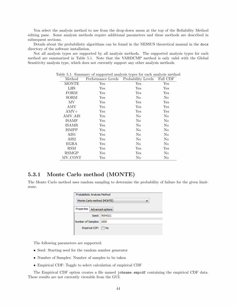
directory of the software installation.Not all analysis types are supported by all analysis methods. The supported analysis types for each
method are summarized in Table 5.1. Note that the VARDCMP method is only valid with the GlobalSensitivity analysis type, which does not currently support any other analysis methods.
Table 5.1: Summary of supported analysis types for each analysis methodMethod Performance Levels Probability Levels Full CDFMONTE Yes Yes Yes
LHS Yes Yes YesFORM Yes Yes YesSORM Yes No No
MV Yes Yes YesAMV Yes Yes Yes
AMV+ Yes Yes YesAMV AIS Yes No No
ISAMF Yes No NoISAMR Yes No NoISMPP Yes No NoAIS1 Yes No NoAIS2 Yes No No
EGRA Yes No NoRSM Yes Yes Yes
RSMGP Yes Yes NoMV CONT Yes No No
5.3.1 Monte Carlo method (MONTE)
The Monte Carlo method uses random sampling to determine the probability of failure for the given limit-state.
The following parameters are supported:
• Seed: Starting seed for the random number generator
• Number of Samples: Number of samples to be taken
• Empirical CDF: Toggle to select calculation of empirical CDF
The Empirical CDF option creates a file named jobname.empcdf containing the empirical CDF data.These results are not currently viewable from the GUI.
44
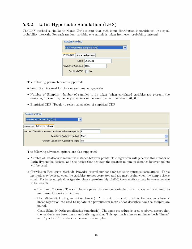
5.3.2 Latin Hypercube Simulation (LHS)
The LHS method is similar to Monte Carlo except that each input distribution is partitioned into equalprobability intervals. For each random variable, one sample is taken from each probability interval.
The following parameters are supported:
• Seed: Starting seed for the random number generator
• Number of Samples: Number of samples to be taken (when correlated variables are present, thesampling process may be very slow for sample sizes greater than about 20,000)
• Empirical CDF: Toggle to select calculation of empirical CDF
The following advanced options are also supported:
• Number of iterations to maximize distance between points: The algorithm will generate this number ofLatin Hypercube designs, and the design that achieves the greatest minimum distance between pointswill be used.
• Correlation Reduction Method: Provides several methods for reducing spurious correlations. Thesemethods may be used when the variables are not correlated and are most useful when the sample size issmall. For large sample sizes (greater than approximately 10,000) these methods may be too expensiveto be feasible.
– Iman and Conover: The samples are paired by random variable in such a way as to attempt tominimize the rank correlations.
– Gram-Schmidt Orthogonalization (linear): An iterative procedure where the residuals from alinear regression are used to update the permutation matrix that describes how the samples arepaired.
– Gram-Schmidt Orthogonalization (quadratic): The same procedure is used as above, except thatthe residuals are based on a quadratic regression. This approach aims to minimize both “linear”and “quadratic” correlations between the samples.
45

• Augment Initial Latin Hypercube Sample: This option allows the user to add additional samplesto an existing analysis, while maintaining the Latin Hypercube structure. Sample sizes can only beincreased by a factor of two. After running an initial analysis, the sample size is increased by leavingall other options at their original values (including the Number of Samples and Seed) and choosingan augmentation factor. For example, and initial sample of size 1,000 can be doubled by choosingan augmentation factor of 2X. If using an external numerical model, the first 1,000 samples will bedetected as repeats from the restart database.
Limitations
• Very large sample sizes (greater than approximately 20,000) may not be feasible when correlatedvariables are present or when correlation reduction methods are employed (advanced options)
• Specified probability levels are interpolated from the empirical CDF
• A maximum of 50 points will be displayed for the full CDF in results visualization.
5.3.3 First- and Second-Order Reliability Methods (FORM andSORM)
The First- and Second-Order Reliability Methods provide approximate estimates of the failure probability,requiring much less model evaluations than Monte Carlo or Latin Hypercube sampling. These methods searchfor the most probable failure point (MPP) and then compute the reliability based on an approximation tothe limit state at this point.
Currently NESSUS does not provide any settings for these methods, but some options will be providedin a future version. When more control is needed, the user may want to consider using AMV or AMV+,which are based on the same first order solution but provide additional settings.
Limitations
Since FORM and SORM are based on limit state approximations, they can be accurate when the limit stateis highly nonlinear. Multiple local MPP’s may also introduce error. These inaccuracies tend to be mostpronounced for large probabilities of failure.
5.3.4 Mean Value methods (MV, AMV, AMV+)
The mean value methods provide very inexpensive approaches to compute probabilities. The mean valuemethod (MV) is based only on the derivatives of the performance function at the mean of the inputs. Theadvanced mean value method (AMV) constructs a first-order Taylor series approximation of the performancefunction at the mean of the inputs and uses this approximation to estimate the MPP. The failure probabilityis then based on a first-order limit state approximation. AMV+ is similar, but additional iterations are usedwhen locating the MPP in order to obtain a more accurate result.
Because all of these methods are based on gradients of the performance function, NESSUS uses finitedifference approximations to estimate these gradients. As shown in Figure 5.3, the user may adjust the sizeof the finite difference steps used on each input. The values entered are in terms of the standard deviation foreach variable. For non-normal variables, care should be taken to ensure that the step size is not large enoughto move outside of the feasible range for that variable. For very noisy responses, the user may also addadditional perturbations, in which case the gradients are estimated using a regression approach. Additionalperturbations can be added using the create row icon (second from the left).
The gear icon (far left) can also be used to bring up a dialog box for automatically generating data fromdifferent finite difference schemes. The supported schemes are forward, backward, and central difference.
AMV+ provides some additional options for controlling convergence:
• Allowable Error: a value between 0.0 and 1.0 that specifies the relative error tolerance in terms ofeither β (for forward problems) or Z (for inverse problems) when locating the MPP
46
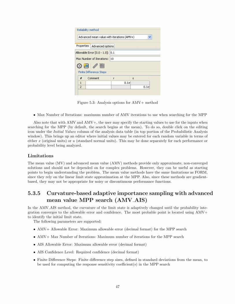
Figure 5.3: Analysis options for AMV+ method
• Max Number of Iterations: maximum number of AMV iterations to use when searching for the MPP
Also note that with AMV and AMV+, the user may specify the starting values to use for the inputs whensearching for the MPP (by default, the search begins at the mean). To do so, double click on the editingicon under the Initial Values column of the analysis data table (in top portion of the Probabilistic Analysiswindow). This brings up an editor where initial values may be entered for each random variable in terms ofeither x (original units) or u (standard normal units). This may be done separately for each performance orprobability level being analyzed.
Limitations
The mean value (MV) and advanced mean value (AMV) methods provide only approximate, non-convergedsolutions and should not be depended on for complex problems. However, they can be useful as startingpoints to begin understanding the problem. The mean value methods have the same limitations as FORM,since they rely on the linear limit state approximation at the MPP. Also, since these methods are gradient-based, they may not be appropriate for noisy or discontinuous performance functions.
5.3.5 Curvature-based adaptive importance sampling with advancedmean value MPP search (AMV AIS)
In the AMV AIS method, the curvature of the limit state is adaptively changed until the probability inte-gration converges to the allowable error and confidence. The most probable point is located using AMV+to identify the initial limit state.
The following parameters are supported:
• AMV+ Allowable Error: Maximum allowable error (decimal format) for the MPP search
• AMV+ Max Number of Iterations: Maximum number of iterations for the MPP search
• AIS Allowable Error: Maximum allowable error (decimal format)
• AIS Confidence Level: Required confidence (decimal format)
• Finite Difference Steps: Finite difference step sizes, defined in standard deviations from the mean, tobe used for computing the response sensitivity coefficient(s) in the MPP search
47

48
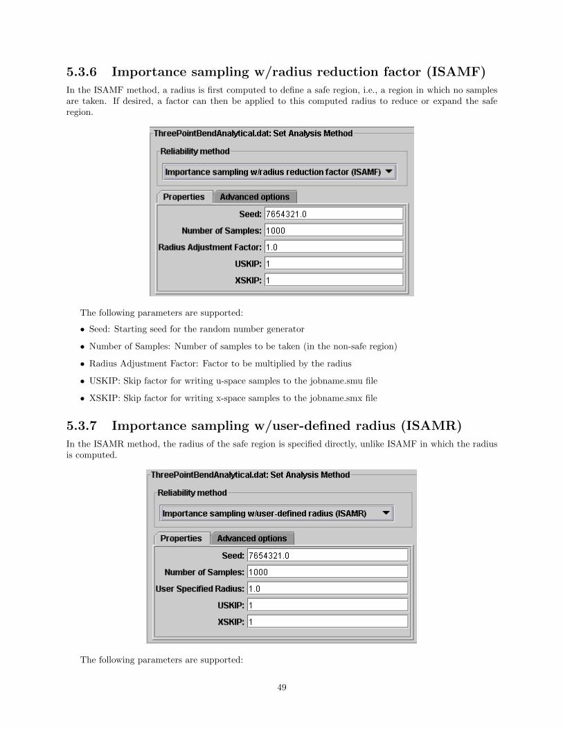
5.3.6 Importance sampling w/radius reduction factor (ISAMF)
In the ISAMF method, a radius is first computed to define a safe region, i.e., a region in which no samplesare taken. If desired, a factor can then be applied to this computed radius to reduce or expand the saferegion.
The following parameters are supported:
• Seed: Starting seed for the random number generator
• Number of Samples: Number of samples to be taken (in the non-safe region)
• Radius Adjustment Factor: Factor to be multiplied by the radius
• USKIP: Skip factor for writing u-space samples to the jobname.smu file
• XSKIP: Skip factor for writing x-space samples to the jobname.smx file
5.3.7 Importance sampling w/user-defined radius (ISAMR)
In the ISAMR method, the radius of the safe region is specified directly, unlike ISAMF in which the radiusis computed.
The following parameters are supported:
49
• Seed: Starting seed for the random number generator
• Number of Samples: Number of samples to be taken (in the non-safe region)
• User Specified Radius: Radius value where no samples are taken within the circle defined by the radius
• USKIP: Skip factor for writing u-space samples to the jobname.smu file
• XSKIP: Skip factor for writing x-space samples to the jobname.smx file
5.3.8 Importance sampling at user-defined MPP (ISMPP)
ISMPP is a basic importance sampling approach that allows the user to specify the location of the importancesampling region. The only difference between the importance sampling density and the actual density of therandom variables is that the mean of the importance sampling density is shifted to the user-defined MPP.
The user may specify a separate MPP for each response level being analyzed. This is done under the SetAnalysis Type editing screen under the Probabilistic Analysis node. The MPP associated with each responselevel is entered in the Initial Values column. Note that the MPP’s are entered in u-space.
The following parameters are supported:
• Seed: Starting seed for the random number generator
• Number of Samples: Number of samples to be taken
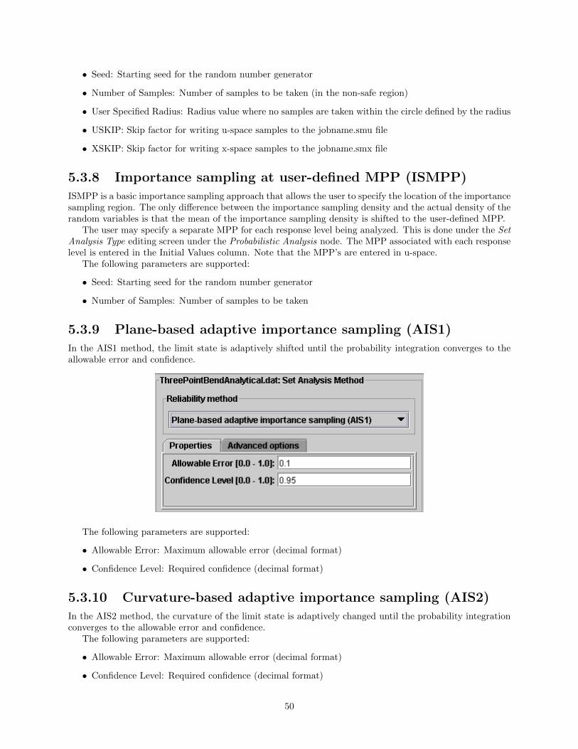
5.3.9 Plane-based adaptive importance sampling (AIS1)
In the AIS1 method, the limit state is adaptively shifted until the probability integration converges to theallowable error and confidence.
The following parameters are supported:
• Allowable Error: Maximum allowable error (decimal format)
• Confidence Level: Required confidence (decimal format)
5.3.10 Curvature-based adaptive importance sampling (AIS2)
In the AIS2 method, the curvature of the limit state is adaptively changed until the probability integrationconverges to the allowable error and confidence.
The following parameters are supported:
• Allowable Error: Maximum allowable error (decimal format)
• Confidence Level: Required confidence (decimal format)
50

5.3.11 Efficient Global Reliability Analysis (EGRA)
EGRA is a powerful method that constructs a Gaussian Process response surface model that is targeted foraccuracy at the limit state. EGRA has the potential to produce very accurate probabilities of failure, evenfor nonlinear limit states, using a small number of samples.
The following options are supported:
• Seed: Starting seed for the random number generator
The following advanced options are also supported:
• Error Based: Whether or not convergence is based on estimated relative error in the failure probability
• Tolerance for Expected Feasibility: When Error Based is not checked, this is a tolerance value thatgoverns when the method will stop adding additional “training points” to the response surface model.Increasing the tolerance may reduce the amount of samples used at the cost of a less accurate responsesurface model.
• Approximate Relative Error: When Error Based is checked, this is a relative tolerance to use onthe failure probability. Note that this is only an approximate error tolerance. This option can addsignificant computational overhead.
• Number of standard deviations to search over: This setting governs how far out into the tails of therandom variables the method will search for new points to add to the response surface model.
• Use Individual Bounds in x-space: Checking this toggle allows the user to individually specify thesearch bounds for each random variable.
• Response Surface Bounds (x-space): This setting only applies when Use Individual Bounds in x-spaceis checked. Here the user enters the search bounds for each random variable in x-space (original units).This option can be particularly useful if the numerical model contains singularities or other instabilitiesthat manifest themselves for particular values of the inputs that are in the tails of the distribution.
• Function noise (std error in absolute units): This setting can be used to improve the algorithm perfor-mance for noisy response functions. Enter an estimate of the magnitude of the noise in the functionoutput. This is interpreted as a standard error.
• Sampling Method: Selects the type of sampling method that is used on the response surface modelwhen computing the probability of failure. The options are:
– Multimodal Adaptive Importance Sampling: The algorithm chooses several “representative”points from among the training points and uses these in an adaptive importance sampling ap-proach that continues sampling until the error has been reduced to a negligible level.
– Multimodal Importance Sampling: This is the same as the Multimodal Adaptive ImportanceSampling approach with the exception that the number of samples used is fixed.
51

– Basic Monte Carlo: A basic Monte Carlo sampling approach is used.
– Use default number of samples: When checked, a default number of samples is used, dependingon the sampling method.
– Number of Samples: Only applies when Use default number of samples is not checked. Thissetting governs the number of samples that are used when sampling the response surface model.For the Multimodal Adaptive Importance Sampling method, this specifies the number of samplesper iteration, but for all other sampling methods this is the total number of samples to be used.
Limitations
• The method may become overly expensive when there is a large number of random variables (approx-imately than 10).
5.3.12 Response Surface Method (RSM)
In the RSM, the original (exact) limit state function is first approximated using one of three experimentaldesigns: Central Composite, Box Behnken, or Koshal (one at a time). The range (level) for each randomvariable can also be specified. Once the original limit state has been approximated, Monte Carlo simulationis used to perform the probabilistic analysis.
The following parameters are supported:
• RSM Settings: Experimental design
• Seed: Starting seed for the random number generator
52

• Error Based: Toggle to select error based solution algorithm
• Number of Samples: Number of samples to be taken
• Allowable Error (error based mode): Maximum allowable error (decimal format)
• Confidence Level (error based mode): Required confidence (decimal format)
• Max Number of Samples (error based mode): Maximum number of samples
• Max WALL Time: Maximum wall time (seconds)
• USKIP: Skip factor for writing u-space samples to the jobname.smu file
• XSKIP: Skip factor for writing x-space samples to the jobname.smx file
• Empirical CDF: Toggle to select calculation of empirical CDF
• Histogram: Toggle to select calculation of histogram
• Number of Bins (histogram mode): Number of bins to use for histogram
5.3.13 Gaussian Process Response Surface Method (RSM GP)
The Gaussian Process Response Surface Method approximates the true limit state function by constructinga Gaussian Process response surface model. The Gaussian Process modeling approach is very flexible and iscapable of accurately modeling a variety of functional forms.
The “training points” used to construct the response surface model are selected randomly over user-specified bounds using Latin Hypercube sampling.
The following parameters are supported:
• Seed: Starting seed for the random number generator
• Number of response surface training points: This is the number of “training points” that will becomputed by evaluating the true limit state function
• Response Surface Bounds (u-space): These are the bounds over which the training points will beselected. Because the response surface model may not be accurate in regions that do not containsufficient training data, choosing bounds that are too small may result in an inaccurate responsesurface model and in turn inaccurate probability results.
• Number of times to sample the response surface: This is the number of samples used to sample theresponse surface model when computing the probability of failure.
5.3.14 Variance Decomposition (VARDCMP)
The variance decomposition method performs a global sensitivity analysis by decomposing the variance ofthe model output with respect to the inputs. This method is only valid when the Global Sensitivity analysistype is selected. Variance decomposition will compute variance-based sensitivity factors for each modelinput.
Three variance decomposition methods are supported:
Structured Monte Carlo An intelligent Monte Carlo sampling scheme is used compute the sensitivityfactors. Note that a large sample size (≈ 1, 000 or more) may be needed to obtain an accuratesolution.
Fourier Amplitude Sensitivity Test The sensitivity factors are computed using a Fourier decomposi-tion.
53

GP with analytical sensitivities Input values are randomly chosen using a Latin Hypercube design andused to construct a Gaussian Process (GP) surrogate model. The variance-based sensitivities are thendetermined exactly based on the surrogate model.
The Sampling Method option is used only by the Structured Monte Carlo method. It determines whatsampling algorithm is used. The recommended choice is “Sobol”, which uses Sobol quasi-random sequences.In most cases, this sampling method provides the fastest convergence and can be used with smaller samplesizes, as compared to Monte Carlo and LHS. Note that the Sobol sequences are deterministic, and the randomnumber seed option is not available. The Monte Carlo and LHS sampling method options are provided forexploring the effect of different sampling methods, and they can also be used to explore the effect of samplingvariability by changing the random number seed.
The Seed option is used to specify the starting seed for random number generation. A special value of0 can be used to generate a time-based seed, so that each run results in a different sequence of randomnumbers.
Number of Samples determines the sample size. For structured Monte Carlo, the total number of modelevaluations will be N(k+2) where N is the user-specified number of samples and k is the number of randomvariables. For the Fourier Amplitude Sensitivity Test, the total number of evaluations is N(k + 1). For theGP model, the total number of evaluations will be N . We recommend using N ≈ 500−10, 000 for structuredMonte Carlo and N ≈ 200 − 2, 000 for the Fourier Amplitude Sensitivity Test. For the GP model, N may
be much smaller, depending on the complexity of the model and the number of random variables; 10√k is a
very approximate rule of thumb.
54
Chapter 6
Results Visualization
6.1 Overview
NESSUS provides powerful capabilities for visualization of results. Some notable featuers are:
• XY plots of the cumulative distribution function and probabilistic sensitivity factors.
• Bar charts of the probabilistic sensitivity factors.
• Pie charts of the probabilistic importance factors.
• User modifiable axis scales including a Log10 scale.
• User modifiable axis and chart titles.
• Support for multiple results sets on the same plot.
• Chart export in multiple file formats.
Results visualization in NESSUS is broken into three categories: Deterministic, Probabilistic, and GlobalSensitivity. When viewing the Visualize Results window, the user can switch between these sections usingthe tabs at the top of the window (although results are only displayed when the corresponding analysishas been run). The user can get to the Visualize Results window either directly from the Deterministic orProbabilistic nodes (by clicking on the Visualize Results button after performing the analysis) or by clickingon the Visualize Results outline node.
6.2 Deterministic Results
When a deterministic analysis is performed, NESSUS generates a set of results containing pre-defined plotconfigurations. Response plots are only available for perturbations that perturb a single variable. A tableof all defined perturbations is available in a tab delimited file named jobname.dst.
Deterministic results can be visualized in tabular form or as XY graphs, as in Figure 6.1. By default theresponse is plotted as a function of each random variable. The random variable values can also be plotted interms of standard deviations by selecting the drop down box under Axes. The individual line plots may beadded or removed by clicking on the corresponding symbol in the legend. Currently plots for this screen areonly generated when the deterministic results contain one-at-a-time parameter variations (i.e. one variableis varied while the others are held at their mean value).
The user selects the response quantity to plot using the drop down menu under the View title. Theavailable responses are those that had to be computed in order to compute the response quantity selectedwhen the analysis was performed. Additional data sets can be plotted on the same graph by adding resultsfiles using the plus button. These results files will be named jobname-deterministic.xml.
The deterministic results can also be viewed in tabular form by selecting the Tabular view button at thebottom of the screen.
55

Figure 6.1: Visualizing deterministic analysis results with an XY plot of each variable in standard normalunits.
56

6.3 Probabilistic Analysis Results Visualization
Probabilistic results are contained under the Probabilistic tab of the Visualize Results window. A full rangeof plots is available for plotting the cumulative distribution function and sensitivity factors. These plots typesare selected using a drop down menu under Type on the visualize results screen (Figure 6.2). Each plot isdescribed below. Additional probabilistic data sets can be plotted on the same graph by adding results filesusing the plus button at the top of the screen. These results files will be named jobname-probabilistic.xml.The probabilistic results can be viewed in tabular form by selecting the Tabular view button at the bottomof the screen.
Figure 6.2: Results visualization for probabilistic analysis
Cumulative Probability
The cumulative probability plot is the cumulative distribution function computed during a probabilisticanalysis. The Y-axis can be either probability or in terms of the standard normal (u).
57
Probabilistic Sensitivity Factors
Probabilistic sensitivity factors are the derivative of the safety index (β) with respect to the mean andstandard deviation of each random variable. This option creates an XY plot of the sensitivity factors as afunction of the response or u value (user selected). For sampling based methods these sensitivity factorsare the derivative of the probability of failure with respect to the mean and standard deviation. Thesesensitivities are normalized by the standard deviation and probability.
Probabilistic Importance Factors
The probabilistic importance factors are the direction cosines to the most probable point in the transformedspace. These factors provide a relative importance of the variables contribution to the probability of failure.These factors are not available for sampling based probabilistic methods. This option creates an XY plot ofthe probabilistic importance factors as a function of the response or u value (user selected).
Probabilistic Importance Factors %
This option creates pie charts of the probabilistic importance factors for each point on the CDF. The Viewdrop down menu allows the selection of the CDF level of interest. The values plotted are α2.
Sensitivity Levels
This option creates bar charts of the probabilistic sensitivity factors. One bar chart is created for each levelon the CDF and the level is selected from the View drop down menu.
Importance Levels
This option creates bar charts of the probabilistic importance factors. One bar chart is created for each levelon the CDF and the level is selected from the View drop down menu.
6.4 Global Sensitivity Results
The Global Sensitivity tab is used to display results obtained from running a probabilistic analysis usingthe Global Sensitivity analysis type. As shown in Figure 6.3, the visualization screen plots two sensitivitymeasures for each variable using a bar chart format: main effects and total effects.
6.5 Chart Formatting Controls
NESSUS now provides full control of axis scales and titles. A right mouse click in the plot area providesaccess to several options including resetting the plot, editing the plot and exporting the plot. The editingscreens follow (see Figure 6.4). The user can change the chart titles, the X and Y-axis scale and titles. TheX-axis can also use a Log10 scale. Finally, the user can also control the placement of the legend.
6.6 Viewing Analysis Files
Most files associated with an analysis share the same basename. The View Analysis Files screen is a utilityto enable you to quickly view the text in these files in a dialog window. The files can be quickly viewedin-place by single-clicking on the title, as seen in Figure 6.5. The files can also be viewed in a separatewindow by double-clicking.
58
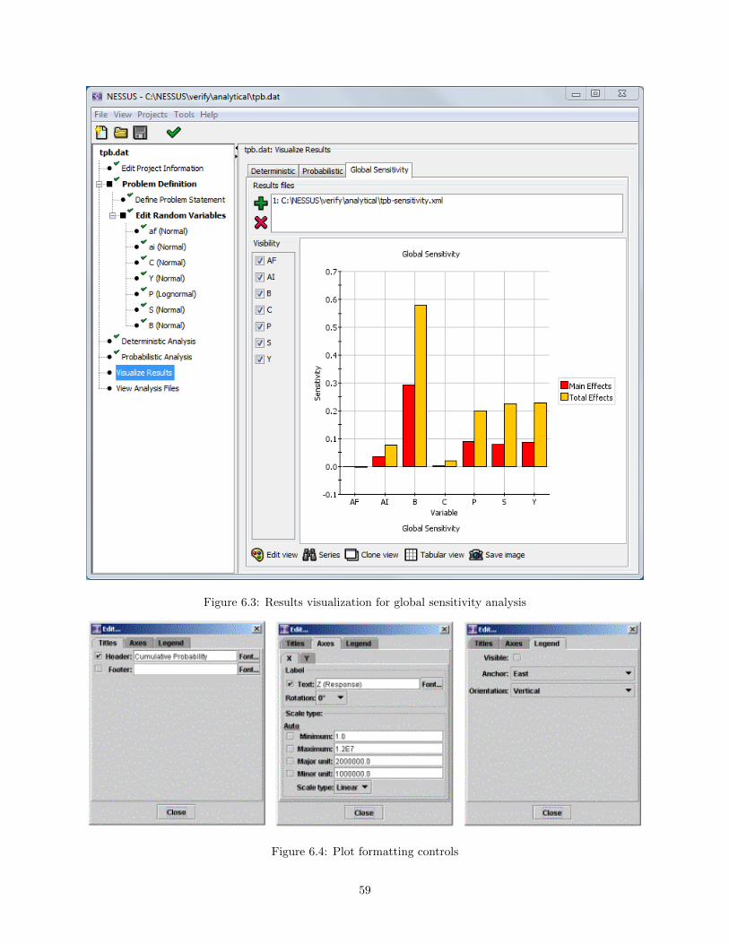
Figure 6.3: Results visualization for global sensitivity analysis
Figure 6.4: Plot formatting controls
59
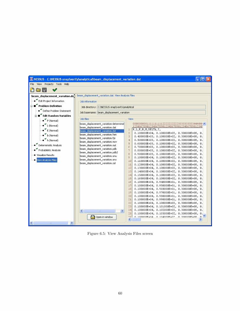
Figure 6.5: View Analysis Files screen
60

Chapter 7
System Requirements
This section describes the system requirements for using NESSUS. Also check the NESSUS web site1 forupdated information.
7.1 Installation
7.1.1 Unix Platforms
On Unix platforms, the NESSUS installer is a self-extracting archive that installs to a directoy named NESSUS
in the current working directory.
7.1.2 Microsoft Windows
On Windows platforms, the NESSUS files are installed to two locations: one for program files and one foruser files. The default installation directory within these locations is NESSUS, but this can be modified duringinstallation.
7.2 Distribution Structure
The NESSUS distribution structure consists of both program and user directories, which vary by systemaccording to Tables 7.1 and 7.2.
Table 7.1: Location of program directoryPlatform Program directory
Unix/Mac NESSUS
Windows 7 C:\Program Files (x86)\NESSUS
Windows XP C:\Program Files\NESSUS
Table 7.2: Location of user directoryPlatform user dir
Unix/Mac NESSUS
Windows 7 C:\Users\Public\Documents\NESSUS
Windows XP C:\Documents and Settings\All Users\Shared Documents\NESSUS
Some of the key directories associated with the installation are:
1See http://www.nessus.com
61
• program dir /bin: NESSUS analysis engine executables
• program dir /docs: NESSUS documentation
• user dir /examples: Example and verification files
• user dir /license: license.txt license file
• user dir /system: NESSUS configuration files
• user dir /training: Files for tutorials and training
7.3 External Analysis Packages
7.3.1 ABAQUS (cf. Section B.1)
ABAQUS is required to perform a NESSUS analysis using ABAQUS to define the performance model.NESSUS expects to execute ABAQUS using the command abaqus. Therefore, this command or a link tothis command is required in the defined path on the system. If for some reason this is not possible anexternal command configuration file can be updated to define the execution command to the desired name.Instructions on how to make these changes can be found in Section 7.4. Note: ABAQUS version 6.5 nolonger supports ABAQUS/CAE on the UNIX platforms therefore the NESSUS/ABAQUS willhave to be performed on either the Windows or Linux platforms for that version of ABAQUS.For the UNIX platforms, an older version of ABAQUS (i.e. version 6.4) will be required forthe NESSUS/ABAQUS interface.
7.3.2 ANSYS (cf. Section B.2)
ANSYS is required to perform a NESSUS analysis using ANSYS to define the performance model. NESSUSexpects to execute ANSYS using the command ansys. Therefore, this command or a link to this commandis required in the defined path on the system. If for some reason this is not possible an external commandconfiguration file can be updated to define the execution command to the desired name. Instructions on howto make these changes can be found in Section 7.4.
NESSUS uses the default ANSYS product defined on the system. If a different product is required thenthis can be set by an environment variable. See the ANSYS documentation for information on setting thedefault product for the specific platform.
7.3.3 LS-DYNA (cf. Section B.3)
LS-DYNA and LSPOST are required to perform a NESSUS analysis using LS-DYNA to define the perfor-mance model. NESSUS expects to execute LSPOST using the command lspost. Therefore, this commandor a link to this command is required in the defined path on the system. If for some reason this is notpossible an external command configuration file can be updated to define the execution command to thedesired name. Instructions on how to make these changes can be found in Section 7.4.
7.3.4 MSC/NASTRAN (cf. Section B.4)
MSC/NASTRAN is required to perform a NESSUS analysis using MSC/NASTRAN to define the perfor-mance model.
7.3.5 MATLAB
MATLAB version 6.5 or greater is required to perform a NESSUS analysis using MATLAB to define theperformance model.
62

7.3.6 USER DEFINED (cf. Section B.6)
The external analysis program must be available on the system. A Fortran compiler is required to compileand link the optional user subroutine for extracting results.
7.4 Updating External Interfaces Configuration File
Several NESSUS interfaces to external analysis programs use the external program for response extraction.For these cases, the external code execution command is required. This execution command is independentof the command to execute the program to complete the analysis. In order to change the default executionvalues for ABAQUS, ANSYS, and LS-DYNA a configuration file named ext_cmd.cfg located in the systemdirectory must be updated. The configuration file uses a keyword followed by the desired execution command.For example, the following keywords and their corresponding commands are initially set in the configurationfile as follows:
ABAQUS_COMMAND abaqus
ANSYS_COMMAND ansys
LS-DYNA_COMMAND lspost -nographics
where,ABAQUS COMMAND is the keyword, andabaqus is the desired execution command.There must be a space between the keyword and execution command.
7.4.1 Example Case
If your system uses the command abq644 instead of abaqus you would change ext_cmd.cfg to:
ABAQUS_COMMAND abq644
Once the desired changes have been implemented just save ext_cmd.cfg and NESSUS will now use theexecution commands defined within the configuration file.
63
Appendix A
Command Line Execution
The NESSUS analysis engine can be executed from the command line without using the graphical userinterface. The NESSUS executable is located in the program directory (see Section 7.2); the relative pathwithin the program directory is system-dependent, but on Windows the executable is bin\w32\nessus.exe.The syntax for running NESSUS from the command line is as follows:
nessus -i INPUT {-d | -p} [-v | -q] [-u USER_DIR] [-l LICENSE] [-r RESPONSE] [--version] [-h]
The symbols {-d | -p} mean that one of either -d or -p is required. Arguments inside square brackets areoptional, and arguments in all capitals denote user-provided values. The individual command line argumentsare explained below:
• -i INPUT: specify the NESSUS input file, without the .dat extension
• {-d | -p}: specify either deterministic (-d) or probabilistic (-p) analysis mode. This argument isrequired.
• [-v | -q]: options for extra verbosity (-v) or quiet output (-q)
• -u USER_DIR: path to user directory portion of installation (required on Windows); see Section 7.2
• -l LICENSE: path to license file, including the filename (if omitted, it is inferred based on the path tothe user directory)
• -r RESPONSE: response variable name (only needed for deterministic analysis)
• --version: show version information and stop
• -h: show command line usage information and stop
For example, the command to run the input file r-s_form in probabilistic analysis mode on Windows 7might look like:
"C:\Program Files (x86)\NESSUS\bin\w32\nessus.exe" -i r-s_form -p -u C:\Users\Public\Documents\NESSUS
Note that quotes are used around the executable path, since it contains spaces.
64

Appendix B
Interfaces
B.1 ABAQUS
B.1.1 Introduction
NESSUS has been integrated with ABAQUS to allow the wide range of deterministic capabilities in ABAQUSto be used within the NESSUS probabilistic framework. ABAQUS is a general-purpose finite elementprogram and is used for analyses modeling a wide range of engineering applications.
NESSUS controls execution of ABAQUS after creating the input file (abaqus job.inp by default). NES-SUS then uses the ABAQUS program to extract results to define the performance for the problem.
65

B.1.2 System Requirements
ABAQUS is required to perform a NESSUS analysis using ABAQUS to define the performance model.NESSUS expects to execute ABAQUS using the command abaqus. Therefore, this command or a link tothis command is required in the defined path on the system. If for some reason this is not possible, anexternal command configuration file can be updated to define the execution command to the desired name.Instructions on how to make these changes can be found in Section 7.4.
B.1.3 Execution Command
The execution command for ABAQUS will be platform specific. A default configuration is provided. Thedestination file name must match the input file in the execution command. NESSUS requires that theABAQUS results be in the abaqus job.odb (this is the default for an ABAQUS analysis with NESSUS).The following figure shows an example.
B.1.4 Responses
NESSUS uses ABAQUS to execute a program that extracts results from the ABAQUS output database(odb) file. A dialogue box consisting of drop down menus and input boxes provides a direct way to definethe NESSUS supported ABAQUS response quantities.
Response Extraction
Supported extraction types include NESSUS defined and User Defined.
Result Type
Supported result types for ABAQUS currently include field data and history data.
Instance
Define the instance name for the response. This is a character string defined in the *INSTANCE keyword ofthe deterministic ABAQUS input file. If no name is given on the *INSTANCE keyword, the default instance
66

name is usually the part name with “-1” appended, e.g. Part-1-1. In some cases, ABAQUS also expects thisname to be given in all uppercase.
Step
Define the step name for the response. This is a character string defined in the *STEP keyword of thedeterministic ABAQUS input file. If no name is given on the *STEP keyword, then the step name is typicallyStep-1, Step-2, etc.
Frame (increment)
Frame or increment number in the step. Use “-1” for the last frame.
Response Type
Currently supported response types include:
• Displacements
• Velocities
• Accelerations
• Stresses
• Total Strains
• Plastic Strains
• Nodal Temperature
• Nodal Heat Flux
• Element Temperature
67

Component
Component defines the specific component of the response such as the displacement in the first direction orthe von Mises stress.
Result Location
For element results (e.g. stress and strain), select between “Centroid”, “Integration Point”, and “Node”(the option for retrieving element results at nodes is currently only supported for field data). This option isdisabled for nodal results (e.g. displacement), which are always defined by node numbers.
Node/Element
List of node or element numbers at which to retrieve the specified response. For element results (e.g. stressand strain), this field expects element numbers unless “Result Location” is set to “Node”. For nodal results(e.g. displacement), this field expects node numbers.
The node or element numbers are listed using the dash (-) and comma (,) to indicate ranges and individualvalues. For example:
1-10, 15, 20-25
would select the values 1 through 10, 15, and 20 through 25.
Integration Point
A single integration point is required along with element numbers when element results type is Integrationpoint.
Section Point
A section point for shell elements.
Time Selection
A function to specify the desired time from history data. The following options are available:
• User Specified
• Last
• Maximum Over Time
• Minimum Over Time
• Absolute Maximum Over Time
• Absolute Minimum Over Time
Function
A function definition is required to operate on response quantities selected for multiple nodes or elements.This operation will reduce the response to a singe quantity. Options currently include maximums andminimums.
Time
Select desired time from history data.
68
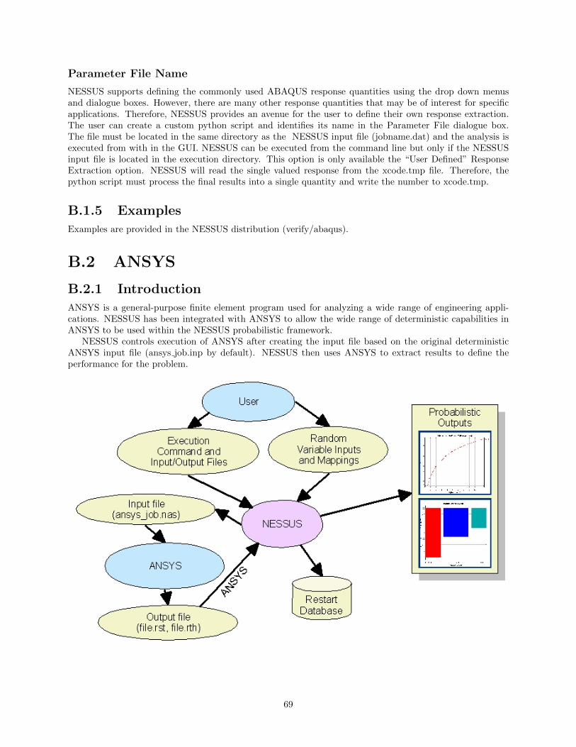
Parameter File Name
NESSUS supports defining the commonly used ABAQUS response quantities using the drop down menusand dialogue boxes. However, there are many other response quantities that may be of interest for specificapplications. Therefore, NESSUS provides an avenue for the user to define their own response extraction.The user can create a custom python script and identifies its name in the Parameter File dialogue box.The file must be located in the same directory as the NESSUS input file (jobname.dat) and the analysis isexecuted from with in the GUI. NESSUS can be executed from the command line but only if the NESSUSinput file is located in the execution directory. This option is only available the “User Defined” ResponseExtraction option. NESSUS will read the single valued response from the xcode.tmp file. Therefore, thepython script must process the final results into a single quantity and write the number to xcode.tmp.
B.1.5 Examples
Examples are provided in the NESSUS distribution (verify/abaqus).
B.2 ANSYS
B.2.1 Introduction
ANSYS is a general-purpose finite element program used for analyzing a wide range of engineering appli-cations. NESSUS has been integrated with ANSYS to allow the wide range of deterministic capabilities inANSYS to be used within the NESSUS probabilistic framework.
NESSUS controls execution of ANSYS after creating the input file based on the original deterministicANSYS input file (ansys job.inp by default). NESSUS then uses ANSYS to extract results to define theperformance for the problem.
69
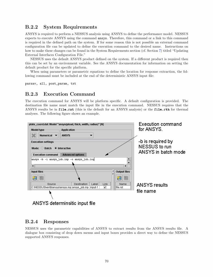
B.2.2 System Requirements
ANSYS is required to perform a NESSUS analysis using ANSYS to define the performance model. NESSUSexpects to execute ANSYS using the command ansys. Therefore, this command or a link to this commandis required in the defined path on the system. If for some reason this is not possible an external commandconfiguration file can be updated to define the execution command to the desired name. Instructions onhow to make these changes can be found in the System Requirements section (cf. Section 7) titled “UpdatingExternal Interfaces Configuration File.”
NESSUS uses the default ANSYS product defined on the system. If a different product is required thenthis can be set by an environment variable. See the ANSYS documentation for information on setting thedefault product for the specific platform.
When using parameters or parametric equations to define the location for response extraction, the fol-lowing command must be included at the end of the deterministic ANSYS input file:
parsav, all, post_param, txt
B.2.3 Execution Command
The execution command for ANSYS will be platform specific. A default configuration is provided. Thedestination file name must match the input file in the execution command. NESSUS requires that theANSYS results be in file.rst (this is the default for an ANSYS analysis) or the file.rth for thermalanalyses. The following figure shows an example.
B.2.4 Responses
NESSUS uses the parametric capabilities of ANSYS to extract results from the ANSYS results file. Adialogue box consisting of drop down menus and input boxes provides a direct way to define the NESSUSsupported ANSYS responses.
70
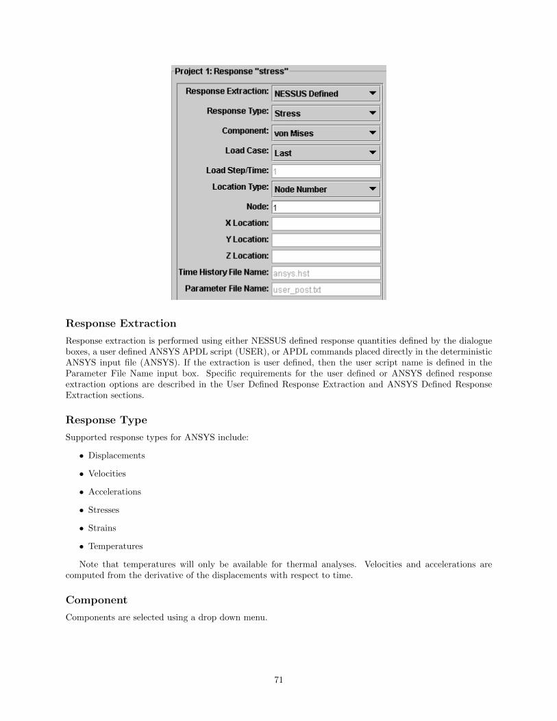
Response Extraction
Response extraction is performed using either NESSUS defined response quantities defined by the dialogueboxes, a user defined ANSYS APDL script (USER), or APDL commands placed directly in the deterministicANSYS input file (ANSYS). If the extraction is user defined, then the user script name is defined in theParameter File Name input box. Specific requirements for the user defined or ANSYS defined responseextraction options are described in the User Defined Response Extraction and ANSYS Defined ResponseExtraction sections.
Response Type
Supported response types for ANSYS include:
• Displacements
• Velocities
• Accelerations
• Stresses
• Strains
• Temperatures
Note that temperatures will only be available for thermal analyses. Velocities and accelerations arecomputed from the derivative of the displacements with respect to time.
Component
Components are selected using a drop down menu.
71
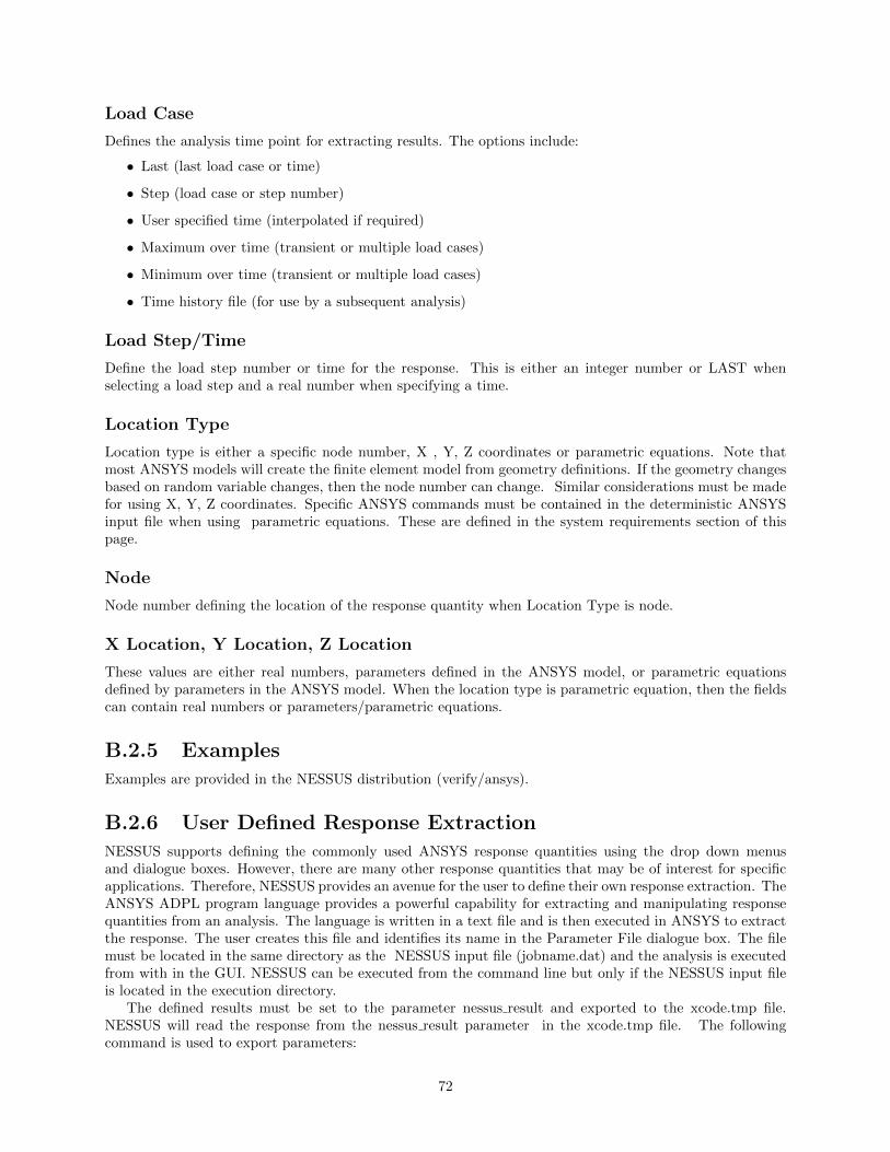
Load Case
Defines the analysis time point for extracting results. The options include:
• Last (last load case or time)
• Step (load case or step number)
• User specified time (interpolated if required)
• Maximum over time (transient or multiple load cases)
• Minimum over time (transient or multiple load cases)
• Time history file (for use by a subsequent analysis)
Load Step/Time
Define the load step number or time for the response. This is either an integer number or LAST whenselecting a load step and a real number when specifying a time.
Location Type
Location type is either a specific node number, X , Y, Z coordinates or parametric equations. Note thatmost ANSYS models will create the finite element model from geometry definitions. If the geometry changesbased on random variable changes, then the node number can change. Similar considerations must be madefor using X, Y, Z coordinates. Specific ANSYS commands must be contained in the deterministic ANSYSinput file when using parametric equations. These are defined in the system requirements section of thispage.
Node
Node number defining the location of the response quantity when Location Type is node.
X Location, Y Location, Z Location
These values are either real numbers, parameters defined in the ANSYS model, or parametric equationsdefined by parameters in the ANSYS model. When the location type is parametric equation, then the fieldscan contain real numbers or parameters/parametric equations.
B.2.5 Examples
Examples are provided in the NESSUS distribution (verify/ansys).
B.2.6 User Defined Response Extraction
NESSUS supports defining the commonly used ANSYS response quantities using the drop down menusand dialogue boxes. However, there are many other response quantities that may be of interest for specificapplications. Therefore, NESSUS provides an avenue for the user to define their own response extraction. TheANSYS ADPL program language provides a powerful capability for extracting and manipulating responsequantities from an analysis. The language is written in a text file and is then executed in ANSYS to extractthe response. The user creates this file and identifies its name in the Parameter File dialogue box. The filemust be located in the same directory as the NESSUS input file (jobname.dat) and the analysis is executedfrom with in the GUI. NESSUS can be executed from the command line but only if the NESSUS input fileis located in the execution directory.
The defined results must be set to the parameter nessus result and exported to the xcode.tmp file.NESSUS will read the response from the nessus result parameter in the xcode.tmp file. The followingcommand is used to export parameters:
72
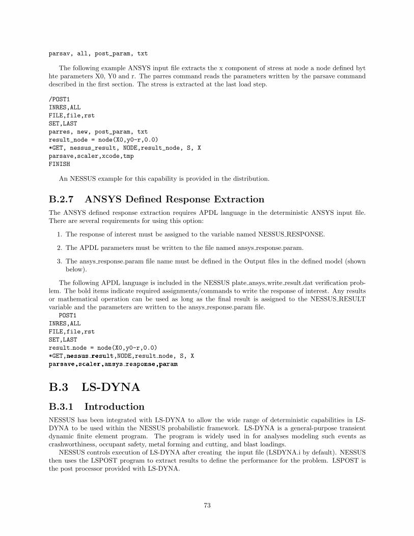
parsav, all, post_param, txt
The following example ANSYS input file extracts the x component of stress at node a node defined bythte parameters X0, Y0 and r. The parres command reads the parameters written by the parsave commanddescribed in the first section. The stress is extracted at the last load step.
/POST1
INRES,ALL
FILE,file,rst
SET,LAST
parres, new, post_param, txt
result_node = node(X0,y0-r,0.0)
*GET, nessus_result, NODE,result_node, S, X
parsave,scaler,xcode,tmp
FINISH
An NESSUS example for this capability is provided in the distribution.
B.2.7 ANSYS Defined Response Extraction
The ANSYS defined response extraction requires APDL language in the deterministic ANSYS input file.There are several requirements for using this option:
1. The response of interest must be assigned to the variable named NESSUS RESPONSE.
2. The APDL parameters must be written to the file named ansys response.param.
3. The ansys response.param file name must be defined in the Output files in the defined model (shownbelow).
The following APDL language is included in the NESSUS plate ansys write result.dat verification prob-lem. The bold items indicate required assignments/commands to write the response of interest. Any resultsor mathematical operation can be used as long as the final result is assigned to the NESSUS RESULTvariable and the parameters are written to the ansys response.param file.
POST1
INRES,ALL
FILE,file,rst
SET,LAST
result node = node(X0,y0-r,0.0)
*GET,nessus result,NODE,result node, S, X
parsave,scaler,ansys response,param
B.3 LS-DYNA
B.3.1 Introduction
NESSUS has been integrated with LS-DYNA to allow the wide range of deterministic capabilities in LS-DYNA to be used within the NESSUS probabilistic framework. LS-DYNA is a general-purpose transientdynamic finite element program. The program is widely used in for analyses modeling such events ascrashworthiness, occupant safety, metal forming and cutting, and blast loadings.
NESSUS controls execution of LS-DYNA after creating the input file (LSDYNA.i by default). NESSUSthen uses the LSPOST program to extract results to define the performance for the problem. LSPOST isthe post processor provided with LS-DYNA.
73
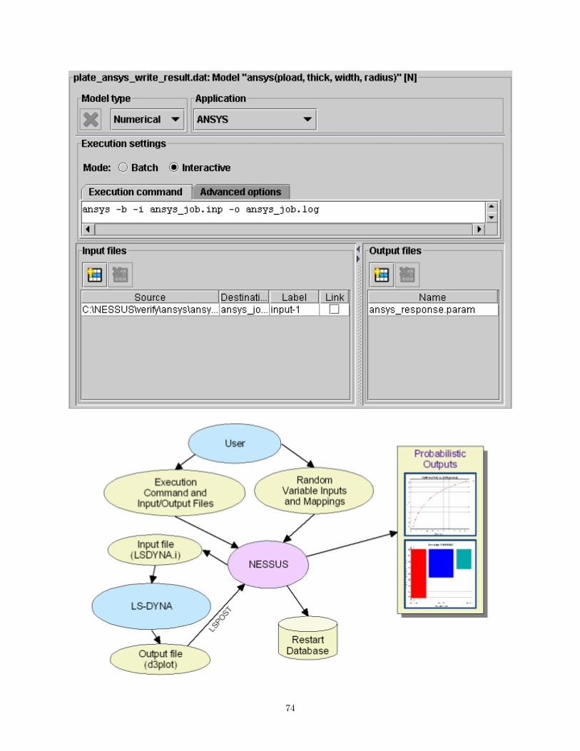
74
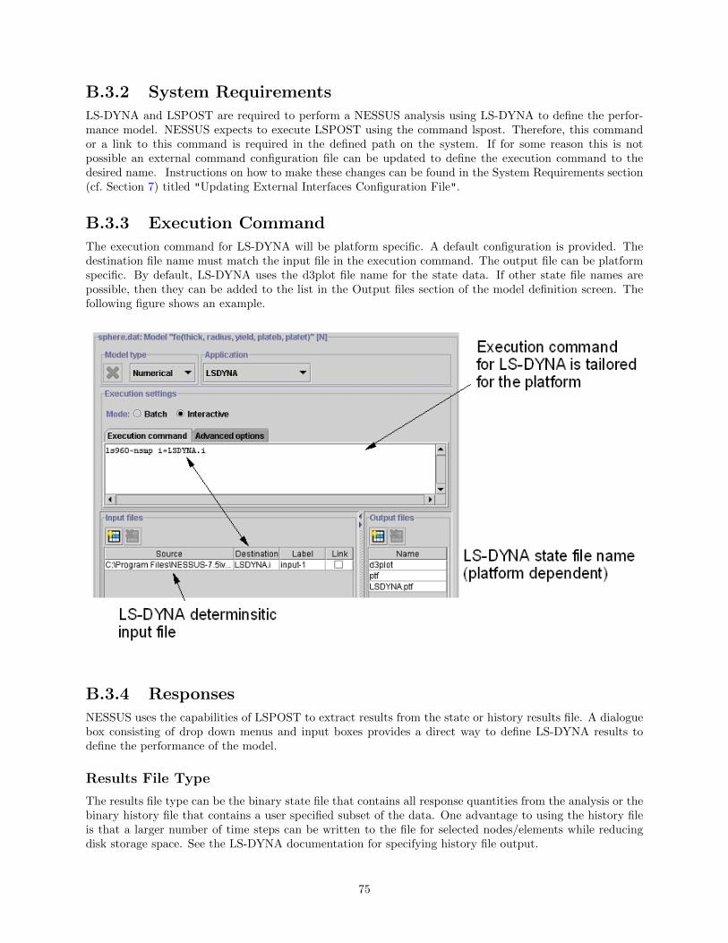
B.3.2 System Requirements
LS-DYNA and LSPOST are required to perform a NESSUS analysis using LS-DYNA to define the perfor-mance model. NESSUS expects to execute LSPOST using the command lspost. Therefore, this commandor a link to this command is required in the defined path on the system. If for some reason this is notpossible an external command configuration file can be updated to define the execution command to thedesired name. Instructions on how to make these changes can be found in the System Requirements section(cf. Section 7) titled "Updating External Interfaces Configuration File".
B.3.3 Execution Command
The execution command for LS-DYNA will be platform specific. A default configuration is provided. Thedestination file name must match the input file in the execution command. The output file can be platformspecific. By default, LS-DYNA uses the d3plot file name for the state data. If other state file names arepossible, then they can be added to the list in the Output files section of the model definition screen. Thefollowing figure shows an example.
B.3.4 Responses
NESSUS uses the capabilities of LSPOST to extract results from the state or history results file. A dialoguebox consisting of drop down menus and input boxes provides a direct way to define LS-DYNA results todefine the performance of the model.
Results File Type
The results file type can be the binary state file that contains all response quantities from the analysis or thebinary history file that contains a user specified subset of the data. One advantage to using the history fileis that a larger number of time steps can be written to the file for selected nodes/elements while reducingdisk storage space. See the LS-DYNA documentation for specifying history file output.
75

76
Result Type
LS-DYNA results are specified as either global, nodal or element type responses. A drop down menu allowsselection of the appropriate result type.
Global Response
Global responses include kinetic, internal, and total energy. A drop down menu allows selection of theresponse.
Nodal Response
Nodal responses include coordinate location, displacements, velocities, and accelerations. A drop down menuallows selection of the response and component. A node number is required for nodal response quantities.Multiple nodes can be input if Curve Average is true.
Element Response
Element responses are specific to the element type (beam, shell ,or hex). A drop down menu allows selectionof the responses for each element type. An element number is required for element response quantities.Multiple elements can be input if Curve Average is true.
Time Selection
Specific time selection is required for transient analyses to define a response for use as the performance inNESSUS
• User specified: input a specific time in the Time input box
• Last: last time in the state or history file
• Maximum over time
• Minimum over time
• Absolute maximum over time
• Absolute minimum over time
• Time history file: a file containing column data for time and response
• Time history file (negative): a file containing column data for time and the negative of the response
• MADYMO function file: A formatted time history file for including in a MADYMO analysis
• MADYMO function file (negative): A formatted time history file with the negative of the response forincluding in a MADYMO analysis
Time
Input a time value when Time Selection is User Specified.
Time History File Name
Enter the time history file name when time selection is Time History or MADYMO function file.
Scale
Allows the response to be scaled by the factor entered in this box. This allows for changing units.
77
Extend Function Time
The function time can be extended for MADYMO function files. This accounts for using LS-DYNA resultsin a MADYMO analysis when there are different ending times for the analysis.
Curve Average
If true, then the response for multiple nodes/elements will be averaged.
Filter
Allows filtering the data using a predefined filter in LSPOST. Filters include SAE, BW, FIR, COS. Thefiltering process is performed after curve averaging.
Filter Time
The time scale for the specified filter. See the LSPOST documentation.
C/s (Hz)
Cycles per second for the specified filter. See the LSPOST documentation.
Output Verbosity
Currently has no effect when using LS-DYNA
B.3.5 Examples
Examples are provided in the NESSUS distribution (verify/ls-dyna).
B.4 MSC.NASTRAN
B.4.1 Introduction
NESSUS has been integrated with NASTRAN to allow the wide range of deterministic capabilities in NAS-TRAN to be used within the NESSUS probabilistic framework.
NESSUS controls execution of NASTRAN after creating the input file (nastran job.inp by default).NESSUS then uses the NASTRAN program to extract results to define the performance for the problem.
B.4.2 System Requirements
NASTRAN is required to perform a NESSUS analysis using NASTRAN to define the performance model.
B.4.3 Execution Command
The execution command for NASTRAN will be platform specific. A default configuration is provided. Thedestination file name must match the input file in the execution command. NESSUS requires that theNASTRAN results be in the nastran job.op2 (this is the default for an NASTRAN analysis with NESSUS).The following figure shows an example. Note: bat=no is required in the execution command to preventNASTRAN from being executed as a background process and to return a code signaling that the NASTRANanalysis has completed. The scr=yes old=no news=no parameters are optional and instruct NASTRANto remove the scratch files, not to save the old files, and not to print the news to the output file. Theseparameters help to reduce disk space usage.
78
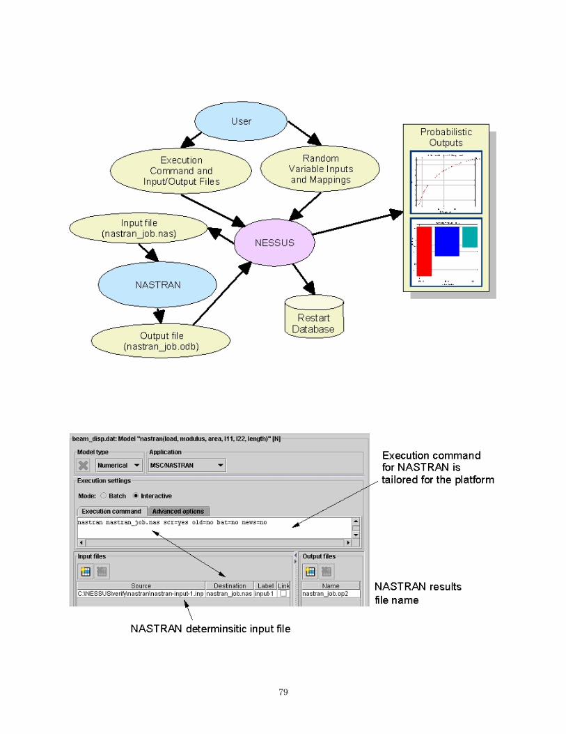
79
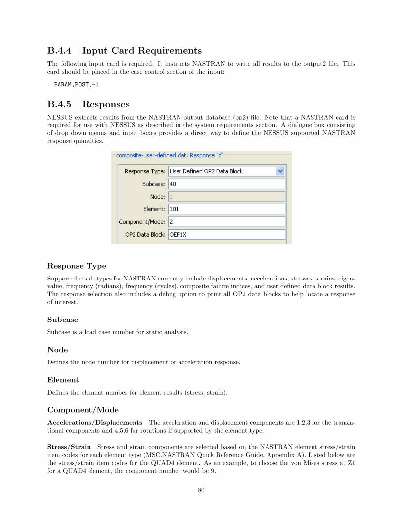
B.4.4 Input Card Requirements
The following input card is required. It instructs NASTRAN to write all results to the output2 file. Thiscard should be placed in the case control section of the input:
PARAM,POST,-1
B.4.5 Responses
NESSUS extracts results from the NASTRAN output database (op2) file. Note that a NASTRAN card isrequired for use with NESSUS as described in the system requirements section. A dialogue box consistingof drop down menus and input boxes provides a direct way to define the NESSUS supported NASTRANresponse quantities.
Response Type
Supported result types for NASTRAN currently include displacements, accelerations, stresses, strains, eigen-value, frequency (radians), frequency (cycles), composite failure indices, and user defined data block results.The response selection also includes a debug option to print all OP2 data blocks to help locate a responseof interest.
Subcase
Subcase is a load case number for static analysis.
Node
Defines the node number for displacement or acceleration response.
Element
Defines the element number for element results (stress, strain).
Component/Mode
Accelerations/Displacements The acceleration and displacement components are 1,2,3 for the transla-tional components and 4,5,6 for rotations if supported by the element type.
Stress/Strain Stress and strain components are selected based on the NASTRAN element stress/strainitem codes for each element type (MSC.NASTRAN Quick Reference Guide, Appendix A). Listed below arethe stress/strain item codes for the QUAD4 element. As an example, to choose the von Mises stress at Z1for a QUAD4 element, the component number would be 9.
80
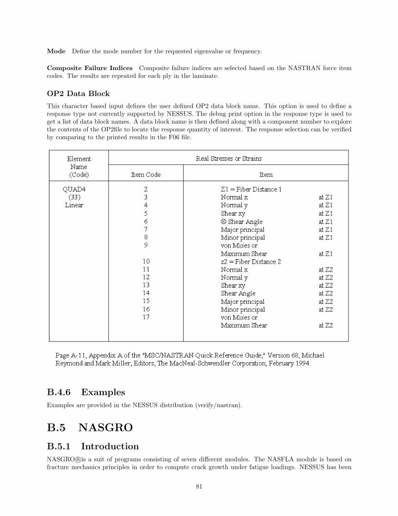
Mode Define the mode number for the requested eigenvalue or frequency.
Composite Failure Indices Composite failure indices are selected based on the NASTRAN force itemcodes. The results are repeated for each ply in the laminate.
OP2 Data Block
This character based input defines the user defined OP2 data block name. This option is used to define aresponse type not currently supported by NESSUS. The debug print option in the response type is used toget a list of data block names. A data block name is then defined along with a component number to explorethe contents of the OP2file to locate the response quantity of interest. The response selection can be verifiedby comparing to the printed results in the F06 file.
B.4.6 Examples
Examples are provided in the NESSUS distribution (verify/nastran).
B.5 NASGRO
B.5.1 Introduction
NASGRO R©is a suit of programs consisting of seven different modules. The NASFLA module is based onfracture mechanics principles in order to compute crack growth under fatigue loadings. NESSUS has been
81
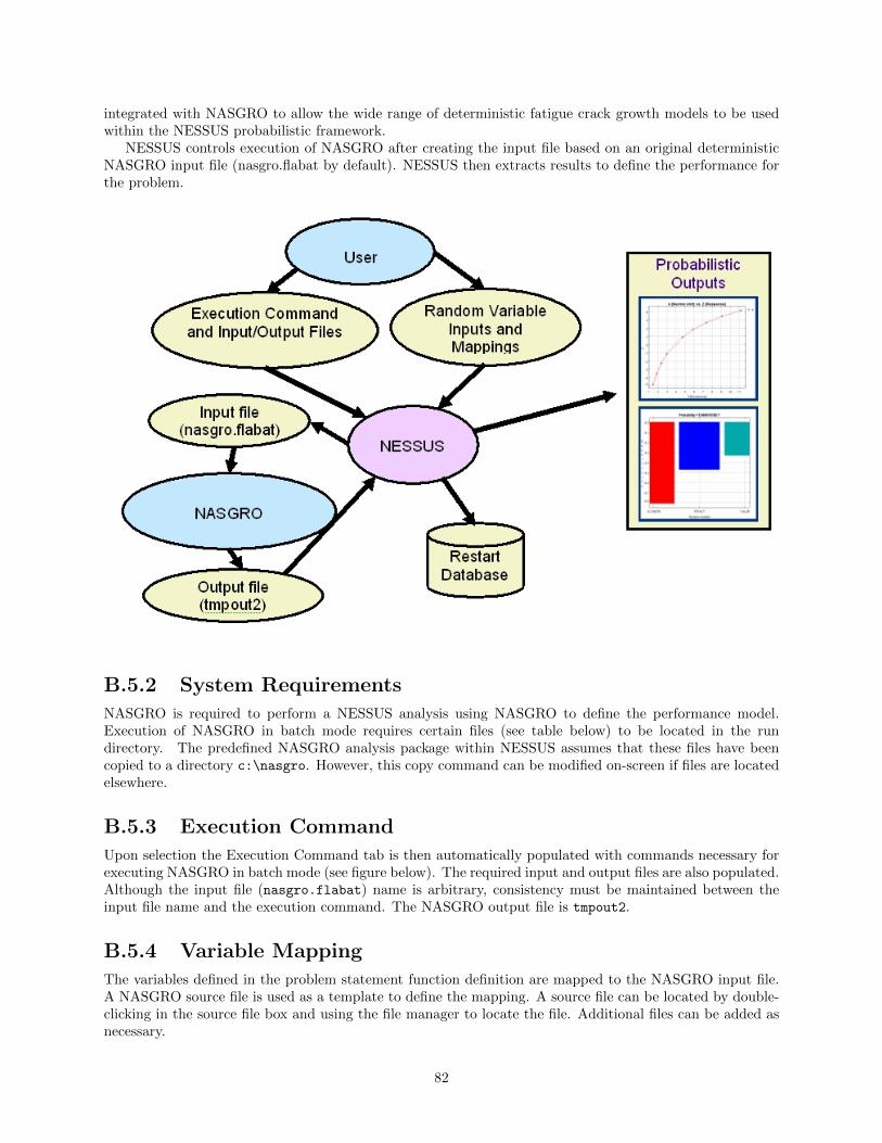
integrated with NASGRO to allow the wide range of deterministic fatigue crack growth models to be usedwithin the NESSUS probabilistic framework.
NESSUS controls execution of NASGRO after creating the input file based on an original deterministicNASGRO input file (nasgro.flabat by default). NESSUS then extracts results to define the performance forthe problem.
B.5.2 System Requirements
NASGRO is required to perform a NESSUS analysis using NASGRO to define the performance model.Execution of NASGRO in batch mode requires certain files (see table below) to be located in the rundirectory. The predefined NASGRO analysis package within NESSUS assumes that these files have beencopied to a directory c:\nasgro. However, this copy command can be modified on-screen if files are locatedelsewhere.
B.5.3 Execution Command
Upon selection the Execution Command tab is then automatically populated with commands necessary forexecuting NASGRO in batch mode (see figure below). The required input and output files are also populated.Although the input file (nasgro.flabat) name is arbitrary, consistency must be maintained between theinput file name and the execution command. The NASGRO output file is tmpout2.
B.5.4 Variable Mapping
The variables defined in the problem statement function definition are mapped to the NASGRO input file.A NASGRO source file is used as a template to define the mapping. A source file can be located by double-clicking in the source file box and using the file manager to locate the file. Additional files can be added asnecessary.
82
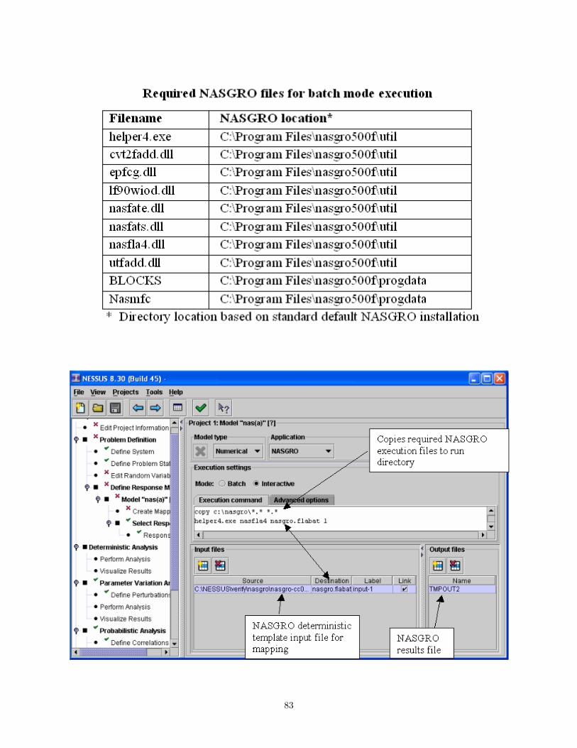
83
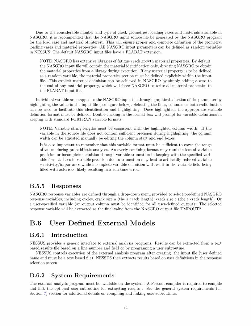
Due to the considerable number and type of crack geometries, loading cases and materials available inNASGRO, it is recommended that the NASGRO input source file be generated by the NASGRO programfor the load case and material of interest. This will ensure proper and complete definition of the geometry,loading cases and material properties. All NASGRO input parameters can be defined as random variablesin NESSUS. The default NASGRO input files have a FLABAT extension.
NOTE: NASGRO has extensive libraries of fatigue crack growth material properties. By default,the NASGRO input file will contain the material identification only, directing NASGRO to obtainthe material properties from a library during execution. If any material property is to be definedas a random variable, the material properties section must be defined explicitly within the inputfile. This explicit material definition can be achieved in NASGRO by simply adding a zero tothe end of any material property, which will force NASGRO to write all material properties tothe FLABAT input file.
Individual variable are mapped to the NASGRO input file through graphical selection of the parameter byhighlighting the value in the input file (see figure below). Selecting the lines, columns or both radio buttoncan be used to facilitate this identification and highlighting. Once highlighted, the appropriate variabledefinition format must be defined. Double-clicking in the format box will prompt for variable definitions inkeeping with standard FORTRAN variable formats.
NOTE: Variable string lengths must be consistent with the highlighted column width. If thevariable in the source file does not contain sufficient precision during highlighting, the columnwidth can be adjusted manually be editing the column start and end boxes.
It is also important to remember that this variable format must be sufficient to cover the rangeof values during probabilistic analyses. An overly confining format may result in loss of variableprecision or incomplete definition through variable truncation in keeping with the specified vari-able format. Loss in variable precision due to truncation may lead to artificially reduced variablesensitivity/importance while incomplete variable definition will result in the variable field beingfilled with asterisks, likely resulting in a run-time error.
B.5.5 Responses
NASGRO response variables are defined through a drop-down menu provided to select predefined NASGROresponse variables, including cycles, crack size a (the a crack length), crack size c (the c crack length). Ora user-specified variable (an output column must be identified for all user-defined output). The selectedresponse variable will be extracted as the final value from the NASGRO output file TMPOUT2.
B.6 User Defined External Models
B.6.1 Introduction
NESSUS provides a generic interface to external analysis programs. Results can be extracted from a textbased results file based on a line number and field or by programing a user subroutine.
NESSUS controls execution of the external analysis program after creating the input file (user definedname and must be a text based file). NESSUS then extracts results based on user definitions in the responseselection screen.
B.6.2 System Requirements
The external analysis program must be available on the system. A Fortran compiler is required to compileand link the optional user subroutine for extracting results . See the general system requirements (cf.Section 7) section for additional details on compiling and linking user subroutines.
84

85
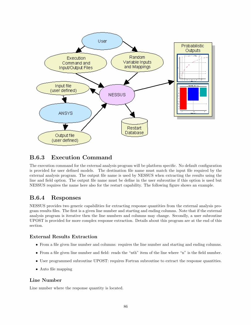
B.6.3 Execution Command
The execution command for the external analysis program will be platform specific. No default configurationis provided for user defined models. The destination file name must match the input file required by theexternal analysis program. The output file name is used by NESSUS when extracting the results using theline and field option. The output file name must be define in the user subroutine if this option is used butNESSUS requires the name here also for the restart capability. The following figure shows an example.
B.6.4 Responses
NESSUS provides two generic capabilities for extracting response quantities from the external analysis pro-gram results files. The first is a given line number and starting and ending columns. Note that if the externalanalysis program is iterative then the line numbers and columns may change. Secondly, a user subroutineUPOST is provided for more complex response extraction. Details about this program are at the end of thissection.
External Results Extraction
• From a file given line number and columns: requires the line number and starting and ending columns.
• From a file given line number and field: reads the “nth” item of the line where “n” is the field number.
• User programmed subroutine UPOST: requires Fortran subroutine to extract the response quantities.
• Auto file mapping
Line Number
Line number where the response quantity is located.
86
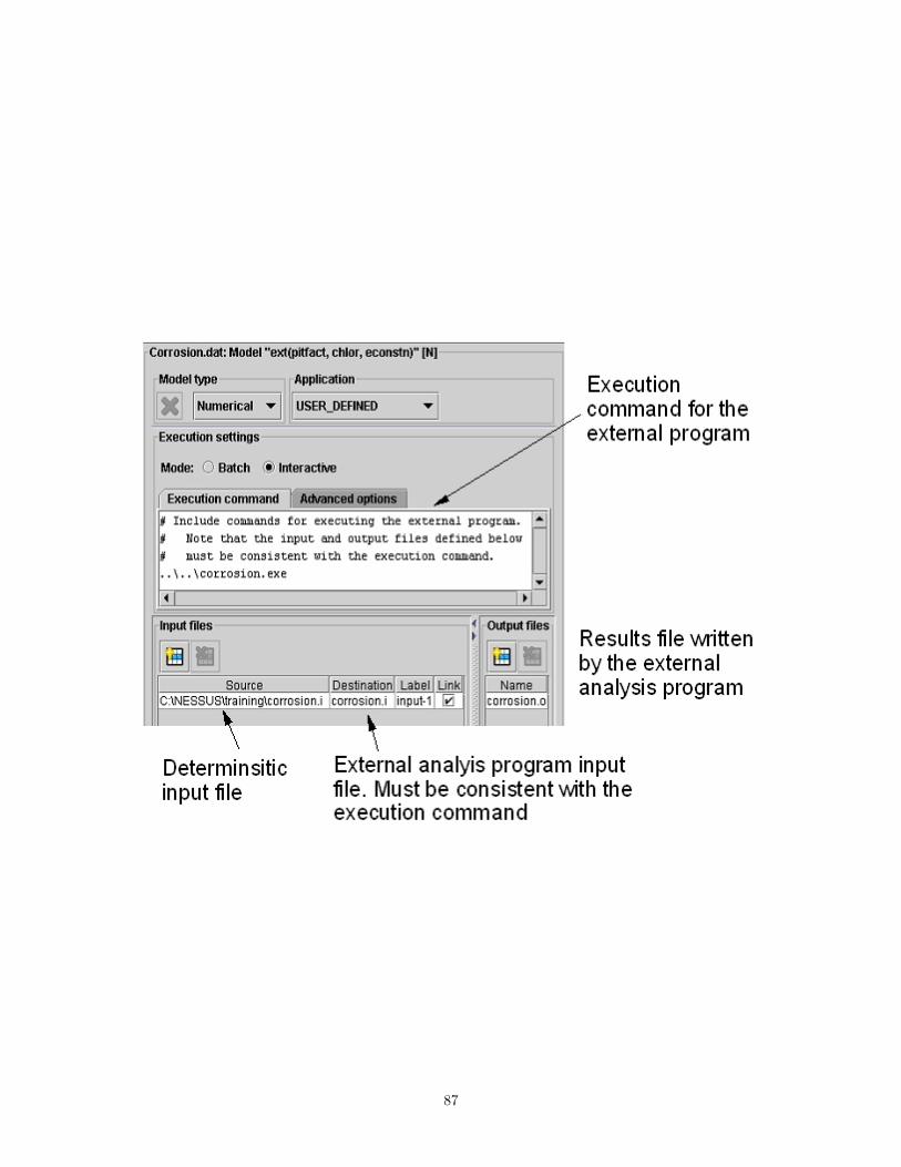
87
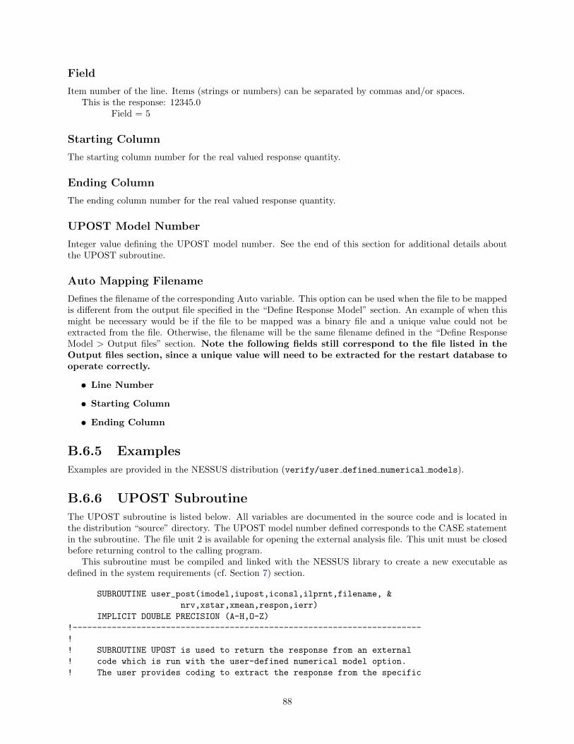
Field
Item number of the line. Items (strings or numbers) can be separated by commas and/or spaces.This is the response: 12345.0
Field = 5
Starting Column
The starting column number for the real valued response quantity.
Ending Column
The ending column number for the real valued response quantity.
UPOST Model Number
Integer value defining the UPOST model number. See the end of this section for additional details aboutthe UPOST subroutine.
Auto Mapping Filename
Defines the filename of the corresponding Auto variable. This option can be used when the file to be mappedis different from the output file specified in the “Define Response Model” section. An example of when thismight be necessary would be if the file to be mapped was a binary file and a unique value could not beextracted from the file. Otherwise, the filename will be the same filename defined in the “Define ResponseModel > Output files” section. Note the following fields still correspond to the file listed in theOutput files section, since a unique value will need to be extracted for the restart database tooperate correctly.
• Line Number
• Starting Column
• Ending Column
B.6.5 Examples
Examples are provided in the NESSUS distribution (verify/user defined numerical models).
B.6.6 UPOST Subroutine
The UPOST subroutine is listed below. All variables are documented in the source code and is located inthe distribution “source” directory. The UPOST model number defined corresponds to the CASE statementin the subroutine. The file unit 2 is available for opening the external analysis file. This unit must be closedbefore returning control to the calling program.
This subroutine must be compiled and linked with the NESSUS library to create a new executable asdefined in the system requirements (cf. Section 7) section.
SUBROUTINE user_post(imodel,iupost,iconsl,ilprnt,filename, &
nrv,xstar,xmean,respon,ierr)
IMPLICIT DOUBLE PRECISION (A-H,O-Z)
!-----------------------------------------------------------------------
!
! SUBROUTINE UPOST is used to return the response from an external
! code which is run with the user-defined numerical model option.
! The user provides coding to extract the response from the specific
88
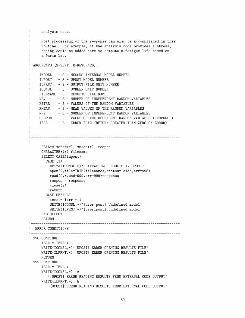
! analysis code.
!
! Post processing of the response can also be accomplished in this
! routine. For example, if the analysis code provides a stress,
! coding could be added here to compute a fatigue life based on
! a Paris law.
!
! ARGUMENTS (S-SENT, R-RETURNED):
!
! IMODEL - S - NESSUS INTERNAL MODEL NUMBER
! IUPOST - S - UPOST MODEL NUMBER
! ILPRNT - S - OUTPUT FILE UNIT NUMBER
! ICONSL - S - SCREEN UNIT NUMBER
! FILENAME - S - RESULTS FILE NAME
! NRV - S - NUMBER OF INDEPENDENT RANDOM VARIABLES
! XSTAR - S - VALUES OF THE RANDOM VARIABLES
! XMEAN - S - MEAN VALUES OF THE RANDOM VARIABLES
! NRV - S - NUMBER OF INDEPENDENT RANDOM VARIABLES
! RESPON - R - VALUE OF THE DEPENDENT RANDOM VARIABLE (RESPONSE)
! IERR - R - ERROR FLAG (RETURN GREATER THAN ZERO ON ERROR)
!
!
!-----------------------------------------------------------------------
!
REAL*8 xstar(*), xmean(*), respon
CHARACTER*(*) filename
SELECT CASE(iupost)
CASE (1)
write(ICONSL,*)’ EXTRACTING RESULTS IN UPOST’
open(2,file=TRIM(filename),status=’old’,err=998)
read(2,*,end=999,err=999)response
respon = response
close(2)
return
CASE DEFAULT
ierr = ierr + 1
WRITE(ICONSL,*)’[user_post] Undefined model’
WRITE(ILPRNT,*)’[user_post] Undefined model’
END SELECT
RETURN
!-----------------------------------------------------------------------
! ERROR CONDITIONS
!-----------------------------------------------------------------------
998 CONTINUE
IERR = IERR + 1
WRITE(ICONSL,*)’[UPOST] ERROR OPENING RESULTS FILE’
WRITE(ILPRNT,*)’[UPOST] ERROR OPENING RESULTS FILE’
RETURN
999 CONTINUE
IERR = IERR + 1
WRITE(ICONSL,*) &
’[UPOST] ERROR READING RESULTS FROM EXTERNAL CODE OUTPUT’
WRITE(ILPRNT,*) &
’[UPOST] ERROR READING RESULTS FROM EXTERNAL CODE OUTPUT’
89
RETURN
END SUBROUTINE user_post
B.7 MATLAB
The MATLAB interface is not enabled in the default NESSUS executable that is distributed to new users.Compiling NESSUS with MATLAB support means that the resulting executable is dependent on severalMATLAB libraries, making it unusable to users that do not have MATLAB installed. To acquire a MATLAB-enabled executable, contact the NESSUS development team at [email protected] with your request.
The MATLAB-enabled executable should then be used to replace the default executable. This can bedone either by replacing the existing executable (preferably after renaming the original) or by copying thenew executable to the bindirectory and using the Preferences menu in the GUI to select the new executable.The remaining instructions for enabling the MATLAB interface are platform-specific and are detailed in thefollowing sections.
B.7.1 Windows
The first step is to install the MATLAB-enabled executable in the proper directory. This is usually inthe C:\Program Files (x86)\NESSUS\bin\w32 directory, but will be different if NESSUS was installedin a non-default location. One option is to replace the existing nessus.exe executable (preferably afterrenaming the original). Alternatively, copy the MATLAB-enabled executable alongside the original, and useTools -> Preferences menu in the NESSUS GUI to select the MATLAB-enabled executable.
Next, the system PATH must be properly set so that the MATLAB libraries on which NESSUS dependscan be located. To set the PATH, open the Start menu, right-click the “My Computer” entry and select“Properties.” On the “Advanced” tab, select “Environment Variables,” then highlight “PATH” and click“Edit.” At the end of the PATH, add a semicolon followed by the required MATLAB directories. This will looksomething like “;C:\Program Files\MATLAB\R2010a\bin;C:\Program Files\MATLAB\R2010a\bin\win32”where “R2010a” should be replaced with your installed version number. This assumes MATLAB was installedin the default location and should be modified if MATLAB is installed in a different location on your system.
The final step is to register MATLAB as a COM server so that NESSUS can launch the MATLAB enginewithout starting MATLAB itself. To do this, open the Start menu, click “Run. . . ” and in the dialog boxthat pops up, type “cmd” and select “OK.” This will open a windows command prompt. At the prompt,type “matlab /regserver” and hit Enter. You can now exit the command prompt by typing “exit” andhitting Enter.
The MATLAB interface is now enabled. For details on how to use the interface, open the NESSUS GUIand use File -> Open Example -> matlab to explore the example problems.
B.7.2 Linux
The first step is to install the MATLAB-enabled executable in the proper directory. NESSUS can be installedin any number of places in Linux, so this will be something like “/path/to/NESSUS/bin/Linux” where youwill need to replace the “/path/to” part with the actual install path on your system.
Next, the LD_LIBRARY_PATH must be properly set so that the MATLAB libraries on which NESSUSdepends can be located. To do this, open a terminal and, if your system is running BASH, type “exportLD_LIBRARY_PATH=/path/to/matlab/bin/glnx86” and hit Enter. On a 64-bit system, replace “glnx86”with “glnxa64.” If you are running a different shell than BASH, the command may be different.
This setting only exists for the current shell session, so after this is set, from this same shell, execute“/path/to/NESSUS/NESSUS.sh” to launch NESSUS and use the MATLAB interface. For details on how touse the interface, see the examples in the NESSUS/verify/matlab directory.
90

B.7.3 Mac OS X
The first step is to install the MATLAB-enabled executable in the proper directory. This is usually inthe “/Applications/NESSUS/bin/Darwin” directory, but will be different if NESSUS was installed in anon-default location.
Next, the DYLD_LIBRARY_PATH must be properly set so that the MATLAB libraries on which NESSUSdepends can be located. To do this, open a Terminal (/Applications/Utilities/Terminal.app) and type“export DYLD_LIBRARY_PATH=/Applications/MATLAB_R2010a.app/bin/maci” and hit Enter. Be sure toreplace “R2010a” with the version you have installed and replace “maci” with “maci64” on 64-bit systems.
This setting only exists for the current Terminal session, so after this is set, from this same shell, execute“open /Applications/NESSUS/NESSUS.app” to launch NESSUS and use the MATLAB interface. For detailson how to use the interface, see the examples in the NESSUS/verify/matlab directory.
91

Appendix C
Problem Statement BNF Grammar
The following text is the language grammar for the problem statement in BNF notation.Statements ::= ( ( Declaration | Assignment ) ( ( <EOL> )+ | <EOF> ) )*Assignment ::= ( Tuple <ASSIGN> Function | Variable <ASSIGN> ( Function | Expression ) )Declaration ::= Function <ASSIGN> ExpressionExpression ::= AdditiveExpAdditiveExp ::= MultiplicativeExp ( <PLUS> MultiplicativeExp | <MINUS> MultiplicativeExp )*MultiplicativeExp ::= ( UnaryExp ( <MULTIPLY> UnaryExp | <DIVIDE> UnaryExp | <MOD>
UnaryExp | <EXPN> UnaryExp )* )UnaryExp ::= ( <MINUS> UnaryExp ) | ( <LPAREN> Expression <RPAREN> | Constant |
Intrinsic | Variable )Intrinsic ::= <INTRINSIC> <LPAREN> Expression <RPAREN>Constant ::= ( <INTEGER LITERAL> | <FLOATING POINT LITERAL> )Variable ::= <IDENTIFIER> ( <LBRACKET> Constant <RBRACKET> )?Tuple ::= <LPAREN> Variable ( <COMMA> Variable )* <RPAREN>Function ::= <IDENTIFIER> <LPAREN> ( Variable ( <COMMA> Variable )* )? <RPAREN>
92
Appendix D
NESSUS Tutorials
D.1 Design of Experiment (DOE) Tutorial
D.1.1 Background
A Design of Experiment (DOE) is a structured, organized method for determining the relationship betweenthe variables affecting the response of a function or model. These types of methods try to gain as muchinsight into a problem with a minimal number of function evaluations. NESSUS currently supports thefollowing DOE methods:
• Box-Behnken (up to 7 variables)
• Central Composite (up to 8 variables)
• Two Level Full Factorial (up to 8 variables)
• Three Level Full Factorial (up to 6 variables)
D.1.2 Example Problem
The following simple example problem is used to illustrate how NESSUS can utilize the above-mentionedmethods to develop a response surface.
The fully plastic flexural capacity of a steel beam section may be given as YZ, whereY = The yield strength of steel.Z = Section Modulus of the section.Then, if the applied bending moment at the pertinent section is M, the performance function may be
defined as g(X) = Y Z −M (Ang and Tang, Probability Concepts in Engineering Planning and Design,Vol. II).
This is entered into NESSUS through the problem definition window. In addition, each of the randomvariables are defined in the corresponding table, as seen in Figure D.1
Next under the “Deterministic Analysis” features is used to create the design of experiments. The inputgenerator is used by clicking on the gear icon. For this problem, the “Three Level Full Factorial” design isselected, as shown in Figure D.2.
Once the “Three Level Full Factorial” design is selected, Figure D.3 shows the design generated byNESSUS for the development of the response surface. Finally, the “Perform Analysis” option is selected andNESSUS analyzes the problem statement for each set of input variables. The results can be seen either inthe “Visualize Results” section or in the corresponding .dst file (i.e. ThreeLevel.dst).
Using the results from the three level full factorial analysis, a response surface can be generated throughNESSUS’s regression capability. The first step is to create a new NESSUS input deck where the response“g” is now defined as a function of y, z, and m, as shown in Figure D.4.
93
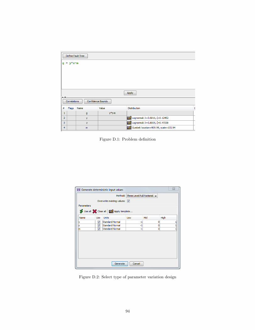
Figure D.1: Problem definition
Figure D.2: Select type of parameter variation design
94
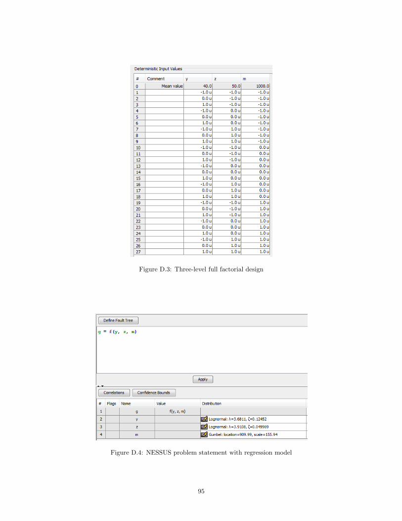
Figure D.3: Three-level full factorial design
Figure D.4: NESSUS problem statement with regression model
95
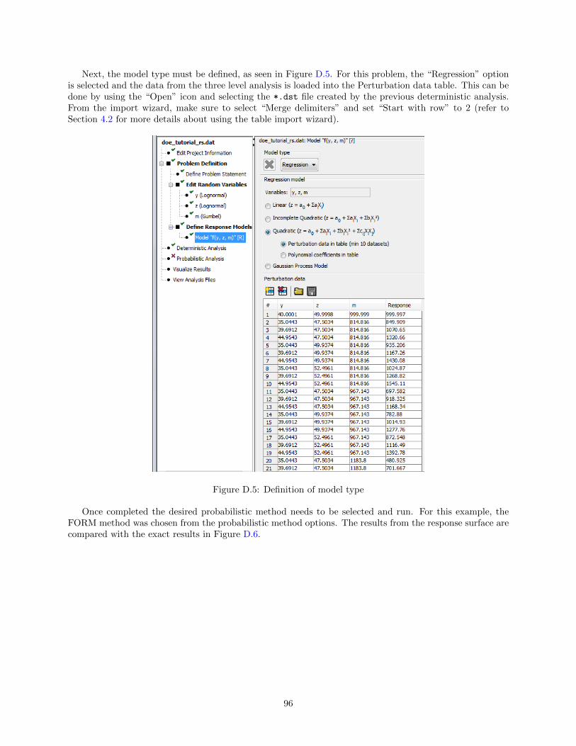
Next, the model type must be defined, as seen in Figure D.5. For this problem, the “Regression” optionis selected and the data from the three level analysis is loaded into the Perturbation data table. This can bedone by using the “Open” icon and selecting the *.dst file created by the previous deterministic analysis.From the import wizard, make sure to select “Merge delimiters” and set “Start with row” to 2 (refer toSection 4.2 for more details about using the table import wizard).
Figure D.5: Definition of model type
Once completed the desired probabilistic method needs to be selected and run. For this example, theFORM method was chosen from the probabilistic method options. The results from the response surface arecompared with the exact results in Figure D.6.
96

Figure D.6: Comparison of results using response surface and exact function
97