Embed Size (px)
Citation preview

Net Present Value Analysis
Andrew Foss([email protected])
Economics 1661 / API-135Environmental and Resource Economics and PolicyHarvard University
February 13, 2009Review Section

Agenda
Fundamental Theories of Welfare Economics
Static Efficiency
Dynamic Efficiency
Cost-Effectiveness Analysis and Benefit / Cost Ratios
Internal Rate of Return
Equivalent Annual Net Benefits
Readings on Benefit-Cost Analysis
Private Goods and Public Goods
Excel Workbook Embedded Here: 2
Microsoft Office Excel 97-2003 Worksheet

Fundamental Theories of Welfare Economics:Pareto Criterion and Pareto Optimality
Pareto Criterion: A policy change is an improvement if at least some people are made better off and no one is made worse off
Pareto Optimality: No other feasible policy could make at least one person better off without making anyone else worse off
3Adam’s Payment
Beth’s Payment
StatusQuo
Policy A
Policy B
Policy C
Policy D
Feasibility Frontier
Possible Payments to Adam and Beth Which satisfy Pareto Criterion?
‒ Policy A does ‒ Policy B does not‒ Policy C does not‒ Policy D does‒ All policies in light gray triangle
Which satisfy Pareto Optimality?
‒ Policy A does not ‒ Policy B does not‒ Policy C does‒ Policy D does‒ All policies on feasibility frontier (because nothing “better” from there)
$25 $100
$25
$100

Fundamental Theories of Welfare Economics:Kaldor-Hicks Criterion
Kaldor-Hicks Criterion: A policy change is an
improvement if the “winners” could fully compensate the
“losers” and still be better off themselves
– Also known as Potential Pareto Improvement Criterion
Kaldor-Hicks Criterion rules out policies with total
benefits smaller than total costs (that is, policies with
negative net benefits, where NB = TB - TC)
When the Kaldor-Hicks Criterion is used to compare all
feasible policy options, the best is that which maximizes
net benefits
– If all policies have negative net benefits, keep the status quo4

0
5
10
15
20
25
0 1 2 3 4 5 6 7 8 9 10
Ma
rgin
al B
en
efi
ts o
r M
arg
ina
l Co
sts
Quantity of Pollution Control
0
20
40
60
80
100
120
0 1 2 3 4 5 6 7 8 9 10
To
tal B
en
efi
ts o
r T
ota
l C
os
ts
Quantity of Pollution Control
Static Efficiency
To achieve static efficiency (single time period),
undertake policy to the point at which marginal
benefits equal marginal costs
5
Total Benefits
Total Costs
Marginal Benefits
Marginal CostsNet Benefits
Q*
Total Benefits and Total Costs Marginal Benefits and Marginal Costs
Q*

Dynamic Efficiency:Overview
To achieve dynamic efficiency (multiple time periods),
undertake policy with highest net present value
If all policies have negative NPV, keep the status quo
Discount rate should reflect social opportunity cost
U.S. Office of Management and Budget (OMB)
published guidance on discount rate and benefit-cost
analysis in Circular A-4 (September 2003):http://www.whitehouse.gov/omb/assets/regulatory_matters_pdf/a-4.pdf
6
T
tttt
r
CB
0 )1(NPV
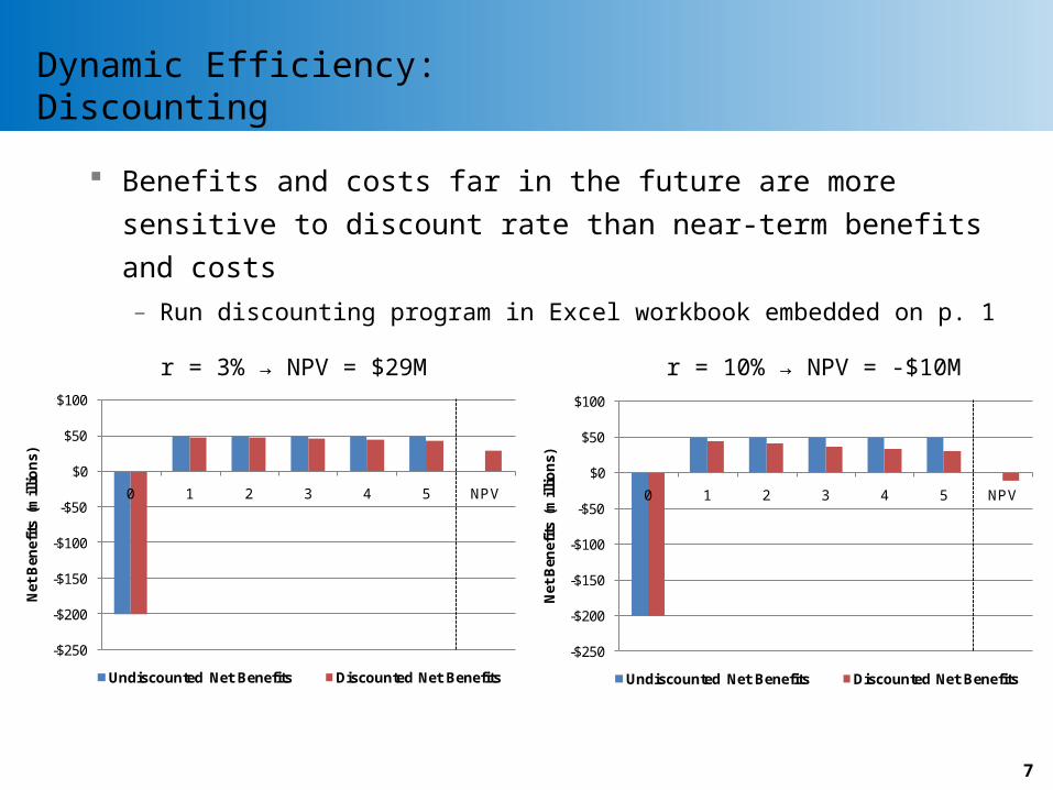
Dynamic Efficiency:Discounting
Benefits and costs far in the future are more sensitive
to discount rate than near-term benefits and costs
– Run discounting program in Excel workbook embedded on p. 1
7
r = 3% → NPV = $29M r = 10% → NPV = -$10M
-$250
-$200
-$150
-$100
-$50
$0
$50
$100
0 1 2 3 4 5 NPV
Net
Ben
efit
s (m
illi
on
s)
Undiscounted Net Benefits Discounted Net Benefits
-$250
-$200
-$150
-$100
-$50
$0
$50
$100
0 1 2 3 4 5 NPV
Net
Ben
efit
s (m
illi
on
s)
Undiscounted Net Benefits Discounted Net Benefits

Dynamic Efficiency:Discounting
When costs are incurred up front and benefits occur in
the future, low discount rates result in higher NPVs than
high discount rates
8
Relationship between Discount Rate and NPVwith Upfront Costs and Future Benefits
-$50
-$40
-$30
-$20
-$10
$0
$10
$20
$30
$40
$50
0% 2% 4% 6% 8% 10% 12% 14% 16% 18% 20%
Net
Pre
sen
t V
alu
e (m
illio
ns)
r

Dynamic Efficiency:Power Plant Example
You are a special assistant to Gov. Schwarzenegger of
California. He wants to shut down a coal-fired power plant
and replace it with either a hydropower plant or a natural gas-
fired plant. He asks you to analyze the options.
Assumptions (unrealistic…)
– Both plants can be built in 1 year and operate for 5 years
– Both plants yield annual benefits of $50M relative to coal
– Hydropower plant has upfront fixed costs of $100M and
annual operating costs of $5M
– Natural gas plant has upfront fixed costs of $40M and
annual operating costs of $20M
– Discount rate is 7 percent, but also try 3 and 10 percent
9
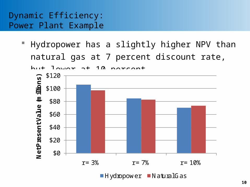
Dynamic Efficiency:Power Plant Example
Hydropower has a slightly higher NPV than natural gas
at 7 percent discount rate, but lower at 10 percent
10
$0
$20
$40
$60
$80
$100
$120
r = 3% r = 7% r = 10%
Ne
t Pre
se
nt
Va
lue
(m
illio
ns
)
Hydropower Natural Gas

Cost-Effectiveness Analysis andBenefit / Cost Ratios
Cost-effectiveness analysis answers the question,
“Does the policy achieve its purpose at least cost?”
Benefits and costs over time should be discounted
When benefits are not monetized, undertake projects
in increasing order of cost per unit of benefit
When benefits are monetized, calculate benefit / cost
ratios and undertake projects in decreasing order of
benefit / cost ratios, provided they are greater than 1
There are problems with both these rules, however11
Qq)(qCi
ii
iiqi
s.t. min

Cost-Effectiveness Analysis andBenefit / Cost Ratios
Cost-effectiveness analysis is less robust than NPV
– Insensitive to scale
– Sensitive to impact definitions (e.g., costs as negative benefits)
12
$0 $20,000
Engine Modifications
Humid Air Motor (HAM)
Direct Water Injection (DWI)
Selective Catalytic Reduction (SCR)
Low-Sulfur Fuel
Shore-side Power
Engine Modifications
Engine Modifications
Engine Modifications
Engine Modifications
Diesel Particulate Filter (DPF) and SCR
Cost-Effectiveness ($/ton NOx)
Oceangoing Vessels
Harbor Craft
Cargo Handling Equipment
Heavy-Duty Vehicles
Locomotives
$11-$50
$280-$350
$450
$540-$790
$3,200
$14,500-$18,500
$1,800
$2,000
$12k-$16k
$1k-$5k
$4k-$14k
Reducing Nitrogen Oxide (NOx) Emissions at Ports‒ Unclear what scale of benefits could result from each measure
‒Unclear to what degree policies should be undertaken
‒ Unclear whether one or several policies should be undertaken
‒ Unclear what probability distributions underlie uncertainty bars

Internal Rate of Return:Overview
Internal rate of return answers the question, “What
discount rate would make NPV zero?”
When costs are incurred up front and benefits occur in
the future, undertake project if IRR > r
In the first discounting example (p. 7), IRR ≈ 8 percent
Internal rate of return is less robust than NPV, and it
should not be used to rank projects when constraints
make it impossible to undertake them all
13
0)1(
NPV0
T
tt
tt
IRR
CB

Internal Rate of Return:Power Plant Example
A nuclear power plant can be built in 1 year for $100M, can operate
for 5 years, yields annual benefits of $55M relative to coal, has
annual operating costs of $5M, and has decommissioning costs of
$155M in Year 6
14-$6
-$5
-$4
-$3
-$2
-$1
$0
$1
$2
$3
0% 2% 4% 6% 8% 10% 12% 14% 16% 18% 20%
Net
Pre
sen
t V
alu
e (m
illio
ns)
r
IRR??
IRR is not useful in this case because there are costs in the future

Equivalent Annual Net Benefits
Suppose the hydropower plant replacing the coal plant
in California can operate for 10 years and the natural
gas plant can still only operate for 5 years
– At r = 7 percent, NPVhydro = $216M and NPVgas = $83M
– At r = 32* percent, NPVhydro = $32M and NPVgas = $30M
* This is an unusually high discount rate, but it illustrates the point for the example numbers
Calculate equivalent annual net benefits to compare
these projects of different duration
– At r = 7 percent, EANBhydro = $27M and EANBgas = $16M
– At r = 32 percent, EANBhydro = $8M and EANBgas = $9M 15
Trr
rNPVEANB
)1(1

Readings on Benefit-Cost Analysis:Arrow et al. (1996)
Benefit-cost analysis is a important framework for
making regulatory decisions
– Careful consideration of benefits and costs
– Common unit of measurement for disparate impacts (dollars)
– Useful tool for improving effectiveness of regulation
– Techniques for incorporating uncertainty
But benefit-cost analysis should not be the sole basis
for making regulatory decisions
– Consideration of distributional impacts as well
– Perhaps not necessary to perform benefit-cost analysis for
minor regulations
16

Readings on Benefit-Cost Analysis:Goulder and Stavins (2002)
Discounting does not shortchange the future, so long as
an appropriate discount rate is used
– It simply puts current values and future values of benefits and
costs in equivalent monetary terms; apples-to-apples
comparison
– It accounts for time value of money (interest) and not inflation:
rnominal ≈ inflation + rreal
When the “winners” of a policy do not actually
compensate the “losers,” the Kaldor-Hicks criterion
carries less weight
Lowering the discount rate to increase NPV is
problematic because it mixes efficiency and equity 17

Private Goods and Public Goods:Beekeeper and Farmer Example
A beekeeper and a farmer are neighbors. The bee-
keeper’s bees help pollinate the farmer’s orchard.
The beekeeper’s marginal benefit from Q beehives is
MBbeekeeper(Q) = 10 – Q
The beekeeper’s marginal cost is constant at
MCbeekeeper(Q) = 7
The farmer’s marginal benefit from Q beehives is
MBfarmer(Q) = 5 – Q
If the beekeeper ignores impacts on the orchard, how
many beehives will the beekeeper have? What if the
beekeeper takes impacts on the orchard into account? 18

Private Goods and Public Goods:Beekeeper and Farmer Example
If the beekeeper treats the beehives as a private good,
the beekeeper will have 3 beehives
19
0
5
10
15
0 5 10 15
MB
or
MC
Quantity of Beehives
MB_beekeeper MC_beekeeper
Q*
MCbeekeeper
MBbeekeper = MCbeekeeper
10 – Q = 7
Q* = 3 beehives
MBbeekeeper

0
5
10
15
0 5 10 15
MB
or
MC
Quantity of Beehives
MB_beekeeper MC_beekeeper MB_farmer MB_society
Private Goods and Public Goods:Beekeeper and Farmer Example
If the beekeeper treats the beehives as a public good,
the beekeeper will have 4 beehives
– Public goods are underprovided by private decision-making
20
Q*
MBbeekeeper
MCbeekeeper
MBsociety = MBbeekeeper + MBfarmer
(vertical sum of MBs for public goods)
For 0 ≤ Q ≤ 5 (where both MBs ≥ 0),
MBsociety = (10 – Q) + (5 – Q) = 15 – 2Q
MCsociety = MCbeekeeper
MBsociety = MCbeekeeper
15 – 2Q = 7
Q* = 4 beehives
MBsociety
MBfarmer

Private Goods and Public Goods:Beekeeper and Farmer Example
If the beekeeper and farmer can negotiate without
transaction costs, what outcome would we expect?
21
Increasing the number of beehives from 3 to 4 gives the
beekeeper extra benefits of $6.50 (area under MBbeekeeper)
but extra costs of $7 (area under MCbeekeeper), so the
beekeeper’s profit decreases by $0.50
Increasing the number of beehives from 3 to 4 gives the
farmer extra benefits of $1.50 (area under MBfarmer) and
does not impose extra costs on the farmer
By the Coase Theorem, the farmer could give the bee-
keeper between $0.50 and $1.50 to have 4 beehives

Private Goods and Public Goods:Steel Mill and Laundry Example
A steel mill generates $1000 in profits and can install
technology to eliminate its emissions at a cost of $400
A laundry can operate either upwind or downwind of the
steel mill, with different building sizes at the locations
– If the laundry operates upwind of the steel mill,
• It can generate $400* in profits if mill releases emissions
• It can generate $600* in profits if mill releases no emissions* Suppose profits differ even when upwind because emissions depress local economy
– If the laundry operates downwind of the steel mill,
• It can generate $200 in profits if mill releases emissions
• It can generate $1000 in profits if mill releases no emissions
22

Private Goods and Public Goods:Steel Mill and Laundry Example
Laundry Upwind Laundry Downwind
Steel Mill Emissions
Steel Mill $1000 $1000
Laundry $400 $200
Joint $1400 (= $1000 + $400) $1200 (= $1000 + $200)
No Steel Mill Emissions
Steel Mill $600 (= $1000 - $400) $600 (= $1000 - $400)
Laundry $600 $1000
Joint $1200 (= $600 + $600) $1600 (= $600 + $1000)
23
Steel Mill and Laundry Profits

Private Goods and Public Goods:Steel Mill and Laundry Example
What is the socially efficient arrangement?
24
– The socially efficient arrangement has highest joint profits for
the steel mill and laundry
– Joint profits are highest ($1600) when the steel mill has no
emissions and the laundry operates downwind

Private Goods and Public Goods:Steel Mill and Laundry Example
Suppose the steel mill and laundry cannot bargain What arrangement will occur if the steel mill has the right
to release emissions?
25
– The steel mill will release emissions, because its profits are higher if it releases
emissions ($1000) than if it does not ($600)
– The laundry will operate upwind, because its profits are higher if it operates
upwind ($400) than if it operates downwind ($200)
What arrangement will occur if the laundry has the
right to clean air?– The steel mill will have to install the technology to eliminate its emissions, leaving
it with $600 in profits
– The laundry will operate downwind, because its profits are higher if it operates
downwind ($1000) than if it operates upwind ($600)

Private Goods and Public Goods:Steel Mill and Laundry Example
Suppose the steel mill and laundry can bargain costlessly What arrangement will occur if the steel mill has the right
to release emissions?
26
– The laundry can increase its profits from $400 operating upwind with emissions to
$1000 operating downwind without emissions. The laundry is willing to pay the
steel mill up to the difference, $600, to install the technology. The steel mill is
willing to accept anything more than $400, so they make some deal in this range.
What arrangement will occur if the laundry has the
right to clean air?– The steel mill is willing to pay up to $400 to avoid installing the technology, but
the laundry is only willing to accept $600 or more to allow emissions and operate
upwind, so there is no deal.
With bargaining, steel mill installs technology and
laundry operates downwind (the efficient arrangement)
regardless of allocation of rights (Coase theorem)