Embed Size (px)
Citation preview

RESEARCH ARTICLE1010022016JC011993
Net primary productivity estimates and environmentalvariables in the Arctic Ocean An assessment of coupledphysical-biogeochemical modelsYounjoo J Lee12 Patricia A Matrai1 Marjorie A M Friedrichs3 Vincent S Saba4 Olivier Aumont5Marcel Babin6 Erik T Buitenhuis7 Matthieu Chevallier8 Lee de Mora9 Morgane Dessert10John P Dunne11 Ingrid H Ellingsen12 Doron Feldman13 Robert Frouin14 Marion Gehlen15Thomas Gorgues10 Tatiana Ilyina16 Meibing Jin1718 Jasmin G John11 Jon Lawrence19Manfredi Manizza20 Christophe E Menkes5 Coralie Perruche21 Vincent Le Fouest22Ekaterina E Popova19 Anastasia Romanou23 Annette Samuelsen24 Jeuroorg Schwinger25Roland Seferian8 Charles A Stock11 Jerry Tjiputra25 L Bruno Tremblay26 Kyozo Ueyoshi14Marcello Vichi2728 Andrew Yool19 and Jinlun Zhang29
1Bigelow Laboratory for Ocean Sciences East Boothbay Maine USA 2Now at Department of OceanographyNaval Postgraduate School Monterey California USA 3Virginia Institute of Marine Science College of William andMary Gloucester Point Virginia USA 4National Ocean and Atmospheric Administration National Marine FisheriesService Northeast Fisheries Science Center Geophysical Fluid Dynamics Laboratory Princeton University PrincetonNew Jersey USA 5Laboratoire Ocean Climat Exploitation et Application NumeriqueInstitut Pierre-Simon LaplaceCNRSIRDUPMC Universite Pierre et Marie Curie Paris France 6Takuvik Joint International LaboratoryCNRS-Universite Laval Quebec Canada 7School of Environmental Sciences University of East Anglia Norwich UK8Centre National de Recherches Meteorologiques Unite mixte de recherche 3589 Meteo-FranceCNRS ToulouseFrance 9Plymouth Marine Laboratory Plymouth UK 10Laboratoire drsquoOceanographie Physique et Spatiale CNRSIFREMERIRDUBO Institut Universitaire et Europeen de la Mer Plouzane France 11NOAAGeophysical Fluid Dynamics LaboratoryPrinceton New Jersey USA 12SINTEF Fisheries and Aquaculture Trondheim Norway 13NASA Goddard Institute for SpaceStudies New York USA 14Climate Atmospheric Science and Physical Oceanography Division Scripps Institution ofOceanography University of California La Jolla California USA 15Laboratoire des Sciences du Climat et delrsquoEnvironnementInstitut Pierre-Simon Laplace Gif-sur-Yvette France 16Max Planck Institute for Meteorology HamburgGermany 17International Arctic Research Center University of Alaska Fairbanks Alaska USA 18Laboratoty for RegionalOceanography and Numerical Modeling Qingdao National Laboratory for Marine Science and Technology QingdaoChina 19National Oceanography Centre University of Southampton Southampton UK 20Geosciences Research DivisionScripps Institution of Oceanography University of California La Jolla California USA 21Mercator-Ocean Toulouse France22LIttoral ENvironnement et Societes Universite de La Rochelle La Rochelle France 23Department of Applied Physics andApplied Mathematics Columbia University and NASA Goddard Institute for Space Studies New York USA 24NansenEnvironmental and Remote Sensing Centre and Hjort Centre for Marine Ecosystem Dynamics Bergen Norway 25UniResearch Climate Bjerknes Centre for Climate Research Bergen Norway 26Department of Atmospheric and OceanicSciences McGill University Montreal Canada 27Department of Oceanography University of Cape Town Cape TownSouth Africa 28Marine Research Institute University of Cape Town Cape Town South Africa 29Applied PhysicsLaboratory University of Washington Seattle Washington USA
Abstract The relative skill of 21 regional and global biogeochemical models was assessed interms of how well the models reproduced observed net primary productivity (NPP) andenvironmental variables such as nitrate concentration (NO3) mixed layer depth (MLD) euphotic layerdepth (Zeu) and sea ice concentration by comparing results against a newly updatedquality-controlled in situ NPP database for the Arctic Ocean (1959ndash2011) The models broadly capturedthe spatial features of integrated NPP (iNPP) on a pan-Arctic scale Most models underestimated iNPPby varying degrees in spite of overestimating surface NO3 MLD and Zeu throughout the regionsAmong the models iNPP exhibited little difference over sea ice condition (ice-free versusice-influenced) and bottom depth (shelf versus deep ocean) The models performed relatively well forthe most recent decade and toward the end of Arctic summer In the Barents and Greenland Seasregional model skill of surface NO3 was best associated with how well MLD was reproduced RegionallyiNPP was relatively well simulated in the Beaufort Sea and the central Arctic Basin where in situ NPP islow and nutrients are mostly depleted Models performed less well at simulating iNPP in theGreenland and Chukchi Seas despite the higher model skill in MLD and sea ice concentration
Key Points Arctic models underestimated net
primary productivity (NPP) butoverestimated nitrate mixed layerdepth and euphotic depth Arctic NPP model skill was greatest in
low production regions Arctic NPP model skill was
constrained by differentenvironmental factors in differentArctic Ocean regions
Correspondence toY J Leeyleebigeloworg and P A Matraipmatraibigeloworg
CitationLee Y J et al (2016) Net primaryproductivity estimates andenvironmental variables in the ArcticOcean An assessment of coupledphysical-biogeochemical models JGeophys Res Oceans 121 doi1010022016JC011993
Received 25 MAY 2016
Accepted 8 NOV 2016
Accepted article online 14 NOV 2016
VC 2016 The Authors
This is an open access article under the
terms of the Creative Commons
Attribution-NonCommercial-NoDerivs
License which permits use and
distribution in any medium provided
the original work is properly cited the
use is non-commercial and no
modifications or adaptations are made
LEE ET AL ARCTIC PRIMARY PRODUCTIVITY ROUND ROBIN 1
Journal of Geophysical Research Oceans
PUBLICATIONS
respectively iNPP model skill was constrained by different factors in different Arctic Ocean regions Ourstudy suggests that better parameterization of biological and ecological microbial rates (phytoplanktongrowth and zooplankton grazing) are needed for improved Arctic Ocean biogeochemical modeling
1 Introduction
Primary production provides the energy that fuels the Arctic Ocean ecosystem However given the regionalheterogeneity the dramatic seasonal changes and the limited access due to harsh environments it is diffi-cult to obtain a comprehensive picture of the Arctic Oceanrsquos in situ primary production regime Models ofbiogeochemical carbon cycling at various spatialtemporal scales also rely on quantification of the first levelof the marine food chainmdashphytoplankton their biomass and production Current projected changes infuture climate and responses of the Arctic Ocean may indicate either (i) an increase in net primary produc-tion (NPP) due to enhanced light availability as a direct result of sea ice and snow cover loss as well asincreased nutrient fluxes from sub-Arctic waters bottom water by vertical mixing and greater upwelling assea ice extent decreases as well as nutrient input by Arctic rivers and terrestrial ecosystems as temperaturerises [Slagstad et al 2015] or (ii) a decrease of NPP due to nutrient limited conditions with enhanced stratifi-cation (due to ice melt freshwater inflow and thermal warming) increased denitrification and decreasedlight availability (due to more clouds and higher water turbidity from permafrost melt beach erosion river-ine input and wind-driven resuspension) [Wassmann and Reigstad 2011] But not all drivers listed aboveare commonly incorporated in numerical models that are widely used for evaluating future changes in NPPover the entire Arctic region today and under a changing climate
There are two main types of numerical models that have been applied to estimate NPP in the Arctic Oceansatellite-based diagnostic models (reviewed in Babin et al [2015] and International Ocean Colour Coordinat-ing Group (IOCCG) [2015] and assessed in Lee et al [2015]) and process-based coupled dynamic physical-biological models run in either retrospective or predictive modes This latter class of models has beenapplied to improve our understanding of the Arctic Ocean carbon sinks and sources using regional [egDeal et al 2011 Manizza et al 2013 Slagstad et al 2015 Zhang et al 2010c2015] to global [eg Popovaet al 2010 Vancoppenolle et al 2013] ice-ocean-atmosphere carbon cycle simulations In general the mag-nitude vertical extent and seasonal evolution of NPP are simulated largely as a function of temperaturelight nutrient availability and physical forcing (advection mixing and stratification) as well as associatedplanktonic and sea ice food web processes The complexity of the models differs not only in the number ofprocessesdrivers included in model simulations but also in their degree of interactive coupling among oce-anic sea ice atmospheric andor hydrologic processes as well as in their biogeochemical component andspatial resolution on one end this allows for year-round simulations in ice-free and ice-covered waters andfor detailed comparisons with satellite-derived observations at certain times and places At the other endcertain models will lack ecosystem biogeochemical and physical (ie freshwater inputs sea ice concentra-tionextentthickness and stratification) parameterizations and feedbacks important to the Arctic Oceanwhich in turn impact controls on NPP For instance regional models may have more flexibility to includeprocesses that are specific to the Arctic Ocean but are limited by the boundary conditions Global modelson the other hand are independent of the boundary conditions but are often lacking in regional complexi-ty in representation of Arctic processes
Previous primary production intercomparison exercises matched in situ carbon uptake rates with NPP esti-mated mostly from ocean color models (OCMs) [eg Balch et al 1992 Campbell et al 2002 Saba et al2011] and more recently from some coupled biogeochemical ocean general circulation models (BOGCMs)[Carr et al 2006 Friedrichs et al 2009 Saba et al 2010] in various regions of the ocean except the ArcticOcean Popova et al [2012] and Vancoppenolle et al [2013] reported the results from various BOGCMs andEarth System Models (ESMs) that were compared for the Arctic domain against satellite-derived NPP albeitwith known issues These latter two studies found reasonable agreement on the main features of pan-Arcticannual NPP and highlighted the disagreement among the models with respect to nutrient availability andsource as well as which factor light or nutrients controls the present-day and future Arctic Ocean NPP Fur-thermore recent individual model studies emphasized the need to accurately parameterize specific
Journal of Geophysical Research Oceans 1010022016JC011993
LEE ET AL ARCTIC PRIMARY PRODUCTIVITY ROUND ROBIN 2
processes to adequately represent NPP within the Arctic Ocean system such as sea ice physics and biogeo-chemistry [eg Jin et al 2012 2016 Tedesco and Vichi 2014] circulation patterns [eg Popova et al 2013]and secondary production [Slagstad et al 2015]
Models that estimate Arctic Ocean NPP have previously been assessed using annual mean and seasonal var-iations in surface nutrients from the World Ocean Atlas and as indicated above ocean color-derived NPPBabin et al [2015] and IOCCG [2015] extensively review the strengths (pan-Arctic weekly or monthly regularcoverage) and limitations (time and space composite imagery sea ice cloudfog seasonal darkness bio-optical and physiological considerations mostly surface observations) of remotely sensed data in this sea-sonally dark and ice-covered region More recently Lee et al [2015] assessed the skill of 32 OCMs to repro-duce the observed NPP across the Arctic Ocean Overall OCMs were most sensitive to uncertainties insurface chlorophyll-a concentration (hereafter chlorophyll) generally performing better with in situ chloro-phyll than with ocean color-derived values Regardless of type or complexity most OCMs were not able tofully reproduce the variability of in situ NPP whereas some of them exhibited almost no bias As a groupOCMs overestimated mean NPP however this was partly offset by some models underestimating NPPwhen a subsurface chlorophyll maximum was present OCMs performed better reproducing NPP valueswhen using Arctic-relevant parameter values
Sampling difficulties and the resulting biogeochemical data scarcity in the Arctic Ocean affect vertical hori-zontal and temporal interpolations frequently used for BOGCM and ESM validation and skill assessmentsuch that only basin-wide temporally averaged (ie annual) data are often used to evaluate their NPP esti-mates While sampling irregularity in the Arctic Ocean even in summer has a strong effect on the spatio-temporal distribution of in situ biogeochemical data it is the increasing availability of such data in recentyears that currently makes the assessment of BOGCM and ESM simulated NPP at smaller and shorter scalesin the Arctic Ocean possible We have assembled a pan-Arctic multidecadal data set of in situ NPP andnitrate (NO3) vertical profiles as well as associated biophysical parameters that allow model skill to beassessed especially at regional scales
NPP observations are herein compared against an available ensemble of physical-biological simulationspresently being applied for a range of global and Arctic-specific carbon and ecosystem questions (Table 1)While model performance of multiple models should ideally be assessed using simulations generated withidentical forcing initialization and boundary conditions such restrictions would severely limit the numberof models considered and fail to sample the variety of present modeling systems Thus in this study in anopportunistic approach 21 model simulations were analyzed within the Arctic domain without forcing theparticipants to use the same setup with the aim of elucidating large-scale similarities and contrasts in NPPand associated drivers Model skill of existing simulations was quantified by assessing modeled integratedNPP (hereafter iNPP) vertical profiles of NPP and NO3 euphotic layer depth (Zeu defined here as the depthat which photosynthetically available radiation (PAR) is 1 of the surface value) mixed layer depth (MLD)and sea ice concentration against in situ or climatological (only MLD) data The participating BOGCMs andESMs include biogeochemical and ecosystem modules of varying complexity that may or may not havebeen optimized for the Arctic Ocean Only Models 9 and 14 include an ice algae component but ice algalproduction was not included in NPP for this study Spatial resolution also varies among the participatingmodels Despite these caveats BOGCMs and ESMs are the only tools that account for complex processes ofland-ocean-atmosphere-sea ice responses to future climate change in the Arctic Ocean Their steadyimprovement requires a regular assessment of their skill to reproduce observations Here we report the firstintercomparison study of NPP in the Arctic Ocean based on 21 simulations from various BOGCMs andESMs against in situ measurements It is a companion study to our earlier assessment of NPP estimatesderived from OCMs [Lee et al 2015]
2 Participating Models
A total of 21 models (Table 1) participated in this exercise 18 of these were coupled ocean-ice-ecosystemmodels (4 Arctic regional and 14 global) and 3 were ESMs The participating models have a horizontal reso-lution between 01 and 200 km with 25ndash75 vertical levels they used various vertical mixing schemes atmo-spheric forcing and sea ice physics (Table 1) Only Model 9 assimilated sea ice concentration and seasurface temperature In terms of biogeochemistry each model has between one and six phytoplankton and
Journal of Geophysical Research Oceans 1010022016JC011993
LEE ET AL ARCTIC PRIMARY PRODUCTIVITY ROUND ROBIN 3
Tab
le1
ABr
iefD
escr
iptio
nof
Part
icip
atin
gM
odel
san
dO
utpu
tVa
riabl
es
Mod
elO
utpu
tVa
riabl
es
Mod
elN
ame
Dom
ain
Type
Hor
izon
tal
Reso
lutio
n(k
m)
Vert
ical
Leve
lsVe
rtic
alM
ixin
gA
tmos
pher
icFo
rcin
gSe
aIc
eN
utrie
nts
of
Phyt
opla
nkto
nC
lass
es
of
Zoop
lank
ton
Cla
sses
of
Det
ritus
Sea
Ice
Biol
ogy
Rive
rN
utrie
nts
Pela
gic-
Bent
hic
Cou
plin
gSi
mul
atio
nPe
riod
Inte
grat
edN
PPN
PP(0
ndash100
m)
NO
3
(0ndash1
00m
)Z e
u
(1
)Se
aIc
eM
LD
1H
YCO
M-
NO
RWEC
OM
Regi
onal
10ndash1
65
28G
ISS
ERA
-Inte
rimre
anal
ysis
Hun
kean
dD
ukow
icz
[199
7]N
PS
i2
23
NY
N19
97ndash2
011
2N
EMO
-PIS
CES
Glo
bal
10ndash1
675
TKE
ERA
-Inte
rimre
anal
ysis
LIM
2N
PS
iFe
22
3N
YY
1998
ndash201
4
3Pl
ankT
OM
53
Glo
bal
013
ndash192
30TK
EN
CEP
rean
alys
isLI
M2
NS
iFe
32
7N
YN
1956
ndash201
3
4
Plan
kTO
M10
Glo
bal
013
ndash192
30TK
EN
CEP
rean
alys
isLI
M2
NP
Si
Fe6
37
NY
N19
48ndash2
013
5M
OM
-SIS
-CO
BALT
Glo
bal
25ndash1
1150
KPP
CO
RE2
GFD
L-SI
SN
PS
iFe
33
1N
YY
1948
ndash200
7
6
MO
M-S
IS-T
OPA
ZG
loba
l25
ndash111
50KP
PC
ORE
2G
FDL-
SIS
NP
Si
FeN
H4
31
7N
YY
1948
ndash200
7
7
SIN
MO
DRe
gion
al20
25Ba
sed
onth
eRi
char
dson
Num
ber
ERA
-Inte
rimre
anal
ysis
Hib
ler
[197
9]
Hun
kean
dD
ukow
icz
[199
7]
NS
i2
22
NY
Y19
79ndash2
014
8N
orES
M-O
CG
loba
l18
ndash65
53TK
EC
ORE
2C
ICE4
NP
Si
Fe1
13
NN
N
1850
ndash201
2
9BI
OM
AS
Regi
onal
3ndash70
30KP
PN
CEP
rean
alys
isTh
ickn
ess
and
enth
alpy
dist
ribut
ion
NS
i2
32
YN
N19
71ndash2
015
10N
EMO
-MED
USA
Glo
bal
68ndash
154
64TK
ED
FS4
1re
anal
ysis
LIM
2N
Si
Fe2
21
NN
N19
88ndash2
006
-
11N
EMO
-ERS
EM(x
honp
)G
loba
l25
ndash68
75TK
EC
ORE
2C
ICE
NP
Si
Fe4
36
NN
Y18
90-2
007
12N
EMO
-ERS
EM(x
honc
)G
loba
l25
-68
75TK
EC
ORE
2C
ICE
NP
Si
Fe4
36
NN
Y18
90ndash2
007
13PE
LAG
OS
Glo
bal
120ndash
160
30TK
EER
A-In
terim
rean
alys
isLI
M2
NP
Si
Fe3
31
NY
N19
88ndash2
010
14IA
RCPO
P-C
ICE
Glo
bal
30ndash4
540
KPP
CO
RE2
CIC
E5
0N
PS
iFe
31
1Y
NN
1958
ndash200
9
15N
EMO
PIS
CES
Glo
bal
63ndash1
3131
TKE
DFS
52
rean
alys
isLI
M2
NP
Si
Fe2
22
NY
Y19
79ndash2
010
16N
EMO
PIS
CES
Glo
bal
3246
TKE
CO
RE2
1N
CEP
D
OE
AM
IP-II
LIM
3N
PS
iFe
22
2N
YN
2002
ndash201
1
17N
EMO
-GEL
ATO
-PI
SCES
Glo
bal
40ndash7
042
TKE
NC
EPre
anal
ysis
GEL
ATO
5N
PS
iFe
22
2N
YY
1948
ndash201
3
18M
ITgc
mRe
gion
al18
50KP
PJR
A25
rean
alys
isH
ible
r[1
979]
N2
22
NY
N19
79ndash2
012
19
Nor
ESM
Glo
balE
SM18
ndash65
53TK
EC
MIP
51
RCP8
5C
ICE4
NP
Si
Fe1
13
NN
N18
50ndash2
012
20
GIS
S-E2
-R-C
CG
loba
lE
SM10
0ndash12
532
KPP
20th
cent
ury
clim
ate
forc
ing
Sea
ice
mod
elE2
NS
iFe
41
3N
NN
1850
ndash201
0
21M
PI-E
SM(M
PIO
M-
HA
MO
CC
)
Glo
bal
ESM
15ndash6
540
Paca
now
skia
ndPh
iland
er[1
981]
1w
ind
mix
ing
CM
IP5
1RC
P45
Not
zet
al[
2013
]N
PS
iFe
11
3N
NY
1850
ndash201
2
Journal of Geophysical Research Oceans 1010022016JC011993
LEE ET AL ARCTIC PRIMARY PRODUCTIVITY ROUND ROBIN 4
zooplankton groups Models use nitro-gen (N) or carbon (C) as currency intheir simulations while phosphorus (P)silica (Si) andor iron (Fe) are includedas state variables in some cases as wellSome models additionally include seaice biology riverine nutrients andorbenthic-pelagic coupling A brief descrip-tion of the models can be found inAppendix A
3 Data and Methods
31 In Situ Net Primary Productivity(NPP 1959ndash2011)We built a quality-controlled in situNPP (mgC m23 d21) database overfive decades (1959ndash2011) that weresampled mostly in the Chukchi Beau-fort and Barents Seas as well as theCanadian Archipelago (Figure 1) Thisdatabase consisted of the ARCSS-PPdata set [Matrai et al 2013] availableat NOAANational Oceanographic DataCenter (NODC) (httpwwwnodcnoaagovcgi-binOASprdaccessiondetails63065) and more recent internationalpolar research activities such as CASES(2004) [Brugel et al 2009 Tremblayet al 2011] ArcticNet (2005ndash2008 and2010ndash2011) (M Gosselin personalcommunication 2014) K-PORT (20072008 and 2010) (S H Lee personalcommunication 2014) CFL (2008)[Mundy et al 2009 Sallon et al 2011]ICE-CHASER (2008) [Charalampopoulouet al 2011] JOIS (2009) [Yun et al2012] RUSALCA (2009) (S H Leepersonal communication 2014) JAM-STEC (2009ndash2010 httpwwwgodacjamstecgojpdarwine) Malina (2009httpmalinaobs-vlfrfr) and ICESCAPE(2010ndash2011 httpseabassgsfcnasagov)[Arrigo et al 2014] These recent datawere primarily collected in the Pacific-sector of the Arctic Ocean (Figure 1c)The in situ sampling stations were select-ed such that discrete NPP measurementsusing 13C or 14C-labeled compoundswere available for at least four discretedepths at each station where the mini-mum depth of in situ NPP was between0 and 5 m in the surface layer Mostof the in situ NPP using a 14C-labeled
(a) 1959minus1989 150ϒ W
120ϒ W
90ϒ W
60ϒ W
30ϒ W
0ϒ
30ϒ E
60ϒ E
90ϒ E
120ϒ E
150ϒ E
180ϒ E
70ϒ N
75ϒ N
80ϒ N
85ϒ N
MarminusJunJulAugSepminusNov
(b) 1990minus1999 150ϒ W
120ϒ W
90ϒ W
60ϒ W
30ϒ W
0ϒ
30ϒ E
60ϒ E
90ϒ E
120ϒ E
150ϒ E
180ϒ E
70ϒ N
75ϒ N
80ϒ N
85ϒ N
MarminusJunJulAugSepminusNov
(c) 2000minus2011 150ϒ W
120ϒ W
90ϒ W
60ϒ W
30ϒ W
0ϒ
30ϒ E
60ϒ E
90ϒ E
120ϒ E
150ϒ E
180ϒ E
70ϒ N
75ϒ N
80ϒ N
85ϒ N
MarminusJunJulAugSepminusNov
Figure 1 The sampling stations where in situ NPP (open circle N 5 928 1959ndash2011)and nitrate (1 N 5 663 1979ndash2011) were measured during the periods of (a) 1959ndash1989(b) 1990ndash1999 and (c) 2000ndash2011 In each plot the stations were also grouped by sea-sons MarchndashJune (green) July (blue) August (black) and SeptemberndashNovember (red)
Journal of Geophysical Research Oceans 1010022016JC011993
LEE ET AL ARCTIC PRIMARY PRODUCTIVITY ROUND ROBIN 5
compound were measured after 24 6 2 h in situ or simulated in situ incubations (N 5 480) and the rest ofthe 14C samples were measured after less than a 12 h incubation or an unknown time period (N 5 397) Insitu carbon uptake rates were also measured using 13C-labeled compounds (N 5 90) after 3ndash6 h on-deckincubations [Lee and Whitledge 2005 Lee et al 2010] A good agreement between estimates of 13C and14C productivity was previously described [Cota et al 1996] Most of the NPP data were reported as dailyvalues but if hourly in situ production rates were reported they were converted to daily production ratesby multiplying with a calculated day length [Forsythe et al 1995] based on the date and location of thesampling stations Note that we did not assess ice algal production in this study due to the scarcity of insitu measurements although sea ice algae may contribute significantly to NPP early in the growth seasonand in certain localities [Fernandez-Mendez et al 2015 Leu et al 2015]
Prior to any integration minimum NPP was set to 025 mgC m23 d21 due to reported methodological preci-sion [Richardson 1991] If the NPP value at the surface (0 m Z0) was not measured it was assumed to bethe same as the closest measurement taken from the uppermost 5 m (Zmin) of the water column In addi-tion if the maximum sampling depth (Zmax) was shallower than 100 m (or bottom depth Zbot) NPP wasextrapolated from Zmax to 100 m (or Zbot) by assuming NPP decreased exponentially Using the multiplesegment trapezoidal rule NPP was integrated from Z0 to 100 m depth as well as alternatively over theeuphotic layer that was determined during the incubation or calculated from available light penetrationdata but in situ Zeu was reported at approximately half of the NPP sampling stations (N 5 519) ice-influenced or ice-free In order to maximize the number of stations available for skill assessment iNPP downto 100 m (or Zbot) was used for analysis since it exhibited only a small difference when compared to iNPPdown to Zeu (r 5 099 plt 001)
Although all the available in situ iNPP ranged between 545 and 18200 mgC m22 d21 at 967 stations out-liers (N 5 39 4) at a confidence level of 95 were removed prior to any analysis due to accuracy issueswith in situ NPP measurements The remaining in situ iNPP data (N 5 928 Figure 2) were between 157 and
1 10 100 1000 100000
20
40
60
iNPP100m
(mgC mminus2 dayminus1)
Num
ber
of s
tatio
ns
(a) fitted logminusnormal distribution
60 70 80 90 00 100
20
40
60
80
Year
(b)
65 70 75 80 85 900
50
100
150
Latitude (oN)
Num
ber
of s
tatio
ns
(c)
A M J J A S O N0
100
200
300
400
Month
(d)
Figure 2 (a) The log-transformed distribution of in situ iNPP (mgC m22 d21) down to 100 m (N 5 927) (b) (c) and (d) show when andwhere those in situ NPP were measured in terms of years latitude and month respectively
Journal of Geophysical Research Oceans 1010022016JC011993
LEE ET AL ARCTIC PRIMARY PRODUCTIVITY ROUND ROBIN 6
5260 mgC m22 d21 (Table 2) with a median value of 246 mgC m22 d21 These iNPP data were log-transformed (base 10) throughout the analysis with a mean of 242 and a standard deviation of 060 (Table2) they exhibited a log-normal distribution (Figure 2a) that was confirmed with the Kolmogorov-Smirnov(K-S) test The majority of available NPP data in the Arctic Ocean was measured after 1975 (Figure 2b) andcollected in the region between 70 and 80N (Figure 2c) mainly from June to September (Figure 2d)
32 In Situ Nitrate (1979ndash2011)Vertical profiles (0ndash100 m) of in situ NO3 were extracted from the NOAANODC ArcNut database [Codispotiet al 2013] (httpwwwnodcnoaagovarchivearc00340072133) as well as additional polar researchcruises at the stations where NPP was measured However in situ NO3 profiles were available only at 663stations (Figure 1) Note that if only combined values of in situ NO3 and nitrite concentration (hereafterNO2) were available those were assumed to be the same as NO3 because NO2 in the Arctic Ocean isextremely low [Codispoti et al 2013] Vertical profiles were sorted by layers (0ndash10 10ndash20 20ndash30 30ndash50 and50ndash100 m) the deepest layer varied depending on station bottom depth and in most cases (approximately70) was measured between 50 and 100 m
33 Sea Ice Concentration (1979ndash2011)Monthly sea ice concentrations () at the corresponding location and date of each NPP station were deter-mined at the nearest grid cell (25 km 3 25 km polar stereographic projection) using NOAANational Snowand Ice Data Center (NSIDC) Climate Data Record of Passive Microwave Sea Ice Concentration Version 2(ftpsidadscoloradoedupubDATASETSNOAAG02202_v2northmonthly) [Meier et al 2013 updated2015 Peng et al 2013] These data files include not only monthly sea ice concentration from July 1987 tothe present but also the merged Goddard Space Flight Center NASA Team [Cavalieri et al 1984] and Boot-strap [Comiso 1986] sea ice concentrations from late 1978 to mid-1987 as an ancillary data set Sea ice con-centration was used to distinguish ice-free (sea ice concentration lt10 which is the NSIDC threshold cut-off for sea ice edge detection in Meier et al [2013 updated 2015]) and ice-influenced (sea ice concentration10) regions Roughly 46 of the NPP stations were located in ice-free waters (N 5 349 Table 2) Amongthe ice-influenced stations (N 5 413) 75 were in marginal ice zones (N 5 175 where sea ice concentrationwas 10ndash50 N 5 136 where sea ice concentration was 50ndash80) and the rest (N 5 102) were in ice-coveredregions (sea ice concentration 80)
34 Mixed Layer Depth (MLD)Because temperature and salinity profile data were often missing or unavailable at the in situ NPP stations(ie separate files archived at different locations) monthly climatological salinity and temperature from thePolar Science Center Hydrographic Climatology (httppscaplwashingtonedunonwp_projectsPHCClima-tologyhtml) [Steele et al 2001] were used to estimate MLD After linearly interpolating the climatologicaltemperature and salinity data in the vertical the monthly climatological MLD was determined at the nearestgrid cell (1 3 1 resolution) for each NPP station by using a threshold criterion of Drh 5 01 kg m23
Table 2 Mean (l) and Standard Deviation (r) of In Situ Log-Transformed iNPP (1959ndash2011 N 5 928) and Depth-Averaged NO3
(1979ndash2011 N 5 663) in Different Regions (Except for Sea Ice Condition During the Period of 1979ndash2011) Periods (Except for NO3 Dur-ing the Period of 1979ndash2011) and Months (Except for March and November)
log(iNPP)iNPP
(mgC m22 d21)Depth-Averaged NO3
(mmol m23)
N l 6 r 10l Range N l 6 r
Regions Sea ice-free 349 242 6 058 263 181ndash5260 273 390 6 305Sea ice-influenced 413 247 6 063 295 157ndash5210 390 376 6 277Shelf 432 251 6 060 321 181ndash5080 244 347 6 291Deep 496 234 6 058 217 157ndash5260 419 403 6 286
Periods Year 1959ndash1989 344 250 6 058 316 194ndash5260 284 509 6 310Year 1990ndash1999 193 261 6 055 404 174ndash5080Year 2000ndash2011 391 225 6 059 177 157ndash4460 379 287 6 230
Months AprilndashJune 201 264 6 059 436 240ndash5260 176 589 6 332July 203 261 6 052 408 249ndash4420 160 327 6 223August 332 239 6 060 244 160ndash5080 182 286 6 228SeptemberndashOctober 186 203 6 045 108 157ndash1570 139 286 6 196All 928 242 6 060 260 157ndash5260 663 382 6 289
Journal of Geophysical Research Oceans 1010022016JC011993
LEE ET AL ARCTIC PRIMARY PRODUCTIVITY ROUND ROBIN 7
[Peralta-Ferriz and Woodgate 2015] where Drh 5 rh(z) 2 rh (5 m) rh(z) and rh(5 m) are the potential densityanomaly (rh 5 qh ndash 1000 kg m23 with qh being potential density) at a given depth (z) and 5 m respectively
35 Model OutputLocation (latitude and longitude) and date of the in situ NPP station data were provided to all modelingteams Each modeling team was then asked to generate monthly mean estimates for vertical profiles(0ndash100 m) of NPP and NO3 iNPP MLD Zeu and sea ice concentration Note that a minimum value for modelNPP was set to 025 mgC m23 d21 similar to the minimum in situ NPP Five models (two global and threeregional) provided daily mean iNPP as well (Models 1 2 3 7 and 9) Unlike iNPP other output variableswere provided by fewer models due to their model setup and configuration (Table 1) For instance Zeu wasonly available in nine participating models Moreover because the simulation period differed among theparticipating models the number of stations used for model-data comparisons varied between N 5 853and N 5 353 (Figure 3) Regardless of the number of in situ stations represented by each model the corre-sponding in situ iNPP were log-normally distributed whereas model estimates were not based on a singlesample K-S test except for Models 2 6 10 and 17 (not shown) Note that the minimum value for modeliNPP was set similar to the minimum in situ value of 545 mgC m22 d21 instead of removing extremely lowor negative values Then analogous to the in situ iNPP approach statistical outliers at a confidence level of95 were discarded in each set of model iNPP output (ie 0ndash10 of model results)
0
100
200
300 (a) 1 (444)
0
50
100(b) 2 (440)
0
100
200(c) 3 (849)
0
100
200
300 (d) 4 (853)
0
100
200(e) 5 (684)
0
100
200(f) 6 (689)
0
100
200 (g) 7 (665)
0
50
100
150 (h) 8 (584)
0
50
100
150
200 (i) 9 (717)
0
100
200 (j) 10 (407)
0
100
200(k) 11 (647)
0
100
200
300 (l) 12 (678)
0
50
100
150 (m) 13 (483)
0
50
100
150 (n) 14 (740)
0
50
100(o) 15 (466)
0
50
100(p) 16 (353)
0
100
200(q) 17 (742)
0
100
200
300 (r) 18 (581)
101 102 103 104 0
50
100(s) 19 (489)
101 102 103 104 0
100
200(t) 20 (801)
101 102 103 104
0
50
100
150(u) 21 (862)
iNPP (mgC mminus2 dayminus1)Num
ber
of o
bser
vatio
ns
101 102 103 104
Figure 3 (andashu) Histogram of simulated (blue monthly mean green daily mean) and in situ iNPP (red mgC m22 d21) Indicated are model numbers in the upper right with the numberof sampling stations in parenthesis which varies due to different simulation periods
Journal of Geophysical Research Oceans 1010022016JC011993
LEE ET AL ARCTIC PRIMARY PRODUCTIVITY ROUND ROBIN 8
36 Model Skill AssessmentA model-data intercomparison of NPP (log-transformed) and NO3 was carried out by assessing the root-mean-square difference (RMSD) from 21 participating models using Target [Jolliff et al 2009] and Taylor[Taylor 2001] diagrams where N is the number of observations in each variable
RMSD25
PNi51 Xi
model2Xiin situ
2
N5bias21uRMSD2
bias5Xmodel 2Xin situ
uRMSD5
ffiffiffiffiffiffiffiffiffiffiffiffiffiffiffiffiffiffiffiffiffiffiffiffiffiffiffiffiffiffiffiffiffiffiffiffiffiffiffiffiffiffiffiffiffiffiffiffiffiffiffiffiffiffiffiffiffiffiffiffiffiffiffiffiffiffiffiffiffiffiffiffiffiffiffiffiffiffiffiffiffiffiffiffiffiffiffiffiffiffiffiffi1N
XN
i51Xi
model2Xmodel
2 Xiin situ2Xin situ
2r
Bias represents the difference between the means of in situ measurement and model output and uRMSDrepresents the difference in the variability between in situ data and model results Hence bias and uRMSDprovide measures of how well mean and variability are reproduced respectively
To visualize bias and uRMSD on a single plot a Target diagram [Jolliff et al 2009] is used after normalizingby the standard deviation (r) of in situ data ie normalized bias (bias) is defined as
bias5bias=rin situ
Although uRMSD is a positive quantity mathematically normalized uRMSD (uRMSD) is also defined in Tar-get diagram as
uRMSD5 uRMSD=rin situ when rmodel gt rin situeth THORN
52uRMSD=rin situ when rmodel lt rin situeth THORN
where rmodel is the standard deviation of Xmodel If uRMSD is positive (negative) the model overestimates(underestimates) the variability of the in situ data In this diagram the closer to the observational reference(the origin) the higher the skill of the model
The Taylor diagram [Taylor 2001] illustrates a different set of statistics in terms of uRMSD that is comprisedof standard deviation (r) of the model output and in situ data as well as the Pearsonrsquos correlation coefficient(r) between model estimates and in situ measurements
uRMSD5
ffiffiffiffiffiffiffiffiffiffiffiffiffiffiffiffiffiffiffiffiffiffiffiffiffiffiffiffiffiffiffiffiffiffiffiffiffiffiffiffiffiffiffiffiffiffiffiffiffiffiffiffiffi11
rmodel2
rin situ2
22 rmodel
rin situ r
s
Note that unlike the Target diagram bias is not illustrated in the Taylor diagram
In addition the Willmott skill (WS) scores [Willmott 1981] were used to quantify an overall regional agree-ment between multimodel mean (ie iNPP NO3 Zeu sea ice concentration and MLD) and observationsand computed as
WS512N RMSD2PN
i51 Ximodel2Xin situ
2 Xi
in situ2Xin situ 2
The highest value WS 51 means perfect agreement between model and observation while the lowestvalue WS 50 indicates disagreement In this study WS is used to quantify model performance in simulat-ing different parameters from various model runs at regional scales However WS may not be usefulwhen in situ data have extremely low variability and zero mean ie when nutrients are depleted becausePN
i51 Ximodel2Xin situ
2 Xi
in situ2Xin situ 2
becomes close to N RMSD2 Moreover since WS is often criti-cized for producing high skill values for entirely uncorrelated signals [Ralston et al 2010] we provide themodeling efficiency (ME) as an alternative validation metric which determines the relative magnitude ofthe residual variance compared to the measured data variance [Nash and Sutcliffe 1970] ME indicateshow well the plot of observed versus simulated regionally averaged data fits the 11 line [Moriasi et al2007] but it can be sensitive to a number of factors such as sample size outliers and magnitude bias[McCuen et al 2006]
Journal of Geophysical Research Oceans 1010022016JC011993
LEE ET AL ARCTIC PRIMARY PRODUCTIVITY ROUND ROBIN 9
ME512RMSD2
r2in situ
The range of ME lies between 10 (perfect fit) and 21 [Stow et al 2009] If ME is zero the model estimatesare as accurate as the mean of the observed data whereas an efficiency less than zero (21ltMElt 0) indi-cates that the observed mean is a better predictor than the model ME can also be illustrated by drawing acircle with a radius equal to one ie ME 5 0 from the origin on the Target diagram For example ME is neg-ative (positive) when a model symbol appears outside (inside) the circle with a radius of one
4 Results
The models broadly captured the spatial features of iNPP on a pan-Arctic scale A majority of the modelsunderestimated iNPP by varying degrees in spite of overestimating surface NO3 MLD and Zeu throughoutthe regions Model skill of iNPP exhibited little difference over sea ice condition and bottom depth Themodels performed equally well on daily versus monthly scales and relatively well for the most recentdecade and toward the end of Arctic summer Much complexity can be seen from the high and sometimesopposing interaction between iNPP and selected physical variables as shown by the variable degree of skillprovided by the different participating models
41 Comparison Between Simulated Daily and Monthly Mean iNPPMost of the models in this intercomparison were only able to provide monthly mean rather than dailymean iNPP In order to determine how the results of this analysis would be affected by using monthly meanmodel output instead of simulated daily iNPP those five models that provided both daily and monthly esti-mates (Models 1 2 3 7 and 9) were compared to each other The distributions of simulated daily andmonthly mean iNPP were very similar in each model (Figures 3andash3c 3f and 3h) and they were strongly cor-related (r 5 083 to 091 plt 001) On average the maximum simulated iNPP was up to 6 higher whencomputed from daily mean values compared to the monthly mean estimates (log-transformed) The stan-dard deviation was higher (4ndash23) when computed from the daily mean iNPP estimates except Model 1However the simulated mean iNPP from those five models computed from the monthly averaged outputwas almost equal or slightly higher (up to 7) than that computed from the daily mean estimates Thisdemonstrates that as expected the monthly averaging smoothed the daily variability while the mean valueexhibited little change Hence results based on the simulated monthly mean iNPP are representative ofhigher temporal resolution data Although the simulated daily mean iNPP exhibited little difference overmonthly averaging the simulated monthly mean iNPP could miss details of the dynamics of NPP on dailytime scales For example no highest estimate from the bloom peak should be shown in model monthlymean output relative to in situ data
42 Model Skill Assessment of iNPP and Depth-Averaged NO3
iNPP was underestimated by most models on a station-by-station basis though not consistently Log-meanvalues of simulated iNPP were mostly negatively biased (Table 3) because the log-distribution of iNPP frommany models was negatively skewed with a longer tail on the left toward low values While the bias wassmall for some models it was very large ie a factor of 10 for others Thirteen out of 21 models reproducediNPP up to 1500 mgC m22 d21 and five others estimated iNPP up to 3000 mgC m22 d21 the remainingthree models simulated iNPP up to 4300 mgC m22 d21 (see Figure 3) while the maximum in situ value was5255 mgC m22 d21 (Table 2) Generally models with large uRMSD ie overestimated variability of iNPP ordepth-averaged NO3 exhibited high standard deviation due to underestimating iNPP (Figure 3) or overesti-mating depth-averaged NO3 (not shown) respectively Unlike iNPP depth-averaged NO3 was positivelybiased in most of the models indicating those models overestimated the mean NO3 in the top 100 m andtheir correlation coefficients were relatively high compared to those of iNPP (Table 3) However no evidentrelationship was found that better model skill in estimating NO3 effected better reproduction of iNPP orvice versa in terms of RMSD (ie combining mean and variability)
43 Model Skill Assessment of iNPP as a Function of Ice Cover Depth Decade and SeasonBased on Table 3 model skill of estimating iNPP was not a function of model domain type or complexity interms of RMSD on a pan-Arctic scale Hence the model skill was examined spatially as a function of sea ice
Journal of Geophysical Research Oceans 1010022016JC011993
LEE ET AL ARCTIC PRIMARY PRODUCTIVITY ROUND ROBIN 10
presence defined from satellite measurements (see section 33) and bottom depth as well as temporally byseasons and simulation periods (Figure 4) While more individual models overestimated mean iNPP (Figure4a) and exhibited a higher correlation coefficient (Figure 4b) in ice-free regions than in ice-influencedregions most models performed nearly equally well in terms of standard deviation between ice-influencedand ice-free regions Indeed as a group model performance was similar regardless of sea ice presence orabsence in terms of both bias and variability ie RMSD Similarly in the case of bottom depth (Zbot) (shelfZbotlt 200 m versus deep ocean Zbotgt 200 m) little difference in model skill was exhibited in terms of bias(Figure 4c) and variability (Figure 4d) Therefore based on the K-S test at a 5 level of significance modelperformance was not significantly different between spatially defined regions (ie ice-free versus ice-influenced and shelf versus deep ocean) in terms of RMSD (not shown)
With respect to temporal scales the performance of models was significantly different between two simula-tion periods 1959ndash1989 and 2000ndash2011 Overall the models performed better in the most recent decade(2000ndash2011) in terms of RMSD whereas most of them significantly underperformed in terms of correlationcoefficient during the earliest decade (r 5 2024 to 024) compared to the latter period (r 5 2019 to 053)(Figure 4f) However no significant difference was found between the two periods in terms of bias only (Fig-ure 4e) based on the K-S test for 5 significance This may be partly due to the fact that more in situ meas-urements have become available in recent years when ice-free conditions have become more pronouncedOn the other hand seasonally estimated iNPP was more negatively biased in the growth period (mean biasof 2112 in AprilndashJune) compared to other seasons (mean bias of 2072 in July 2024 in August and 2023in SeptemberndashOctober) but the models performance was not significantly different between seasons interms of variability (Figures 4g and 4h) This is probably because the models have a seasonal cycle thatalthough slightly shifted early in phase for the Arctic Ocean is still within a reasonable range In additionthe models include a range of approaches to estimating the vertical distribution of irradiance (ie lighttransmission through sea ice) Some models simply scale down shortwave radiation by sea ice concentra-tion whereas others include radiation transmission as a fully coupled and bidirectional formulation (egCICE-based models) Still other models compute light transmission through sea ice as a function of sea icephysics and biogeochemistry For example the Pelagic Interaction Scheme for Carbon and Ecosystem Stud-ies (PISCES)-based models have a complex formulation of the vertical penetration of PAR through the watercolumn which takes into account incoming radiation wavelength chlorophyll-dependent attenuation
Table 3 Mean (l) and Standard Deviation (r) of Estimated iNPP (Log-Transformed) and Depth-Averaged NO3 (mmol m23)a
Model
log(iNPP) Depth-Averaged NO3
N
l r
RMSD Bias uRMSD r N
l r
RMSD Bias uRMSD rIn Situ Modeled In Situ Modeled In Situ Modeled In Situ Modeled
1 444 227 130 059 076 132 2098 089 016 439 321 405 263 171 264 086 250 0392 440 231 202 060 044 067 2029 060 037 445 322 523 265 228 326 202 256 0463 849 240 243 058 042 059 003 059 034 663 382 543 289 229 403 161 370 20014 853 240 232 058 036 063 2008 062 020 663 382 604 289 396 475 223 419 0285 684 253 251 054 029 059 2001 059 010 461 422 367 309 347 270 2054 265 0686 689 252 271 054 027 059 019 056 016 461 422 041 309 041 473 2380 282 0667 665 247 231 060 034 059 2016 057 037 621 389 560 290 276 327 172 278 0528 584 242 231 059 083 092 2011 092 020 436 392 979 303 320 737 587 446 20029 717 244 257 060 051 068 013 067 027 663 382 501 289 488 567 120 554 00510 407 258 250 053 022 055 2008 055 012 392 411 378 309 297 306 2033 304 04911 647 250 181 054 108 143 2069 125 2009 448 426 653 307 209 393 227 321 02712 678 251 182 055 107 142 2069 124 2006 461 422 933 309 318 636 512 377 02813 483 245 213 060 047 071 2032 063 032 493 369 193 293 174 296 2174 239 05714 740 236 218 058 078 088 2018 086 022 578 392 686 296 305 461 295 354 03015 466 244 213 061 036 068 2031 061 028 - - - - - - - - -16 353 226 239 059 050 060 014 059 044 - - - - - - - - -17 742 239 243 058 031 060 003 060 023 550 382 729 300 286 462 348 304 04618 581 237 142 060 083 145 2094 110 2017 548 321 582 245 277 406 262 310 03019 489 247 198 058 072 099 2049 086 013 436 392 1251 303 245 938 859 378 00620 730 239 123 060 039 137 2116 072 2003 585 381 066 278 083 397 2315 242 05621 862 240 196 059 076 098 2044 087 018 - - - - - - - - -
aRMSD bias uRMSD and Pearsonrsquos correlation coefficient (r) are computed between each model estimate and in situ measurement (see Appendix A for details) The number ofstations (N) varies mainly due to different model simulation periods and in situ data availability Note that Models 15 16 and 21 did not provide model estimates of NO3 which is indi-cated by a dash (-)
Journal of Geophysical Research Oceans 1010022016JC011993
LEE ET AL ARCTIC PRIMARY PRODUCTIVITY ROUND ROBIN 11
minus2 minus1 0 1 2 3
minus3
minus2
minus1
0
1
2
Normalized uRMSDN
orm
aliz
ed b
ias
(a)
Sea
minusic
e
iceminusfree (sea ice concentration10)iceminusinfluenced (sea ice concentrationgt10)
10 200
1
2
3
10
20
30
Nor
mal
ized
Sta
ndar
d D
evia
tion
10
20
30
uRMSD
minus040 000030
060
090
100
Correlation Coefficient
(b)
minus2 minus1 0 1 2 3
minus3
minus2
minus1
0
1
2
Normalized uRMSD
No
rmal
ized
bia
s
(c)
Dep
th
shallow (depth200m)deep (depthgt200m)
10 200
1
2
3
10
20
30
Nor
mal
ized
Sta
ndar
d D
evia
tion
10
20
30
uRMSD
minus040 000030
060
090
100
Correlation Coefficient
(d)
minus2 minus1 0 1 2 3
minus3
minus2
minus1
0
1
2
Normalized uRMSD
No
rmal
ized
bia
s
(e)
Dec
ade
1959~19891990minus19992000minus2011
10 200
1
2
3
10
20
30N
orm
aliz
ed S
tand
ard
Dev
iatio
n
10
20
30
uRMSD
minus040 000030
060
090
100
Correlation Coefficient
(f)
minus2 minus1 0 1 2 3
minus3
minus2
minus1
0
1
2
Normalized uRMSD
No
rmal
ized
bia
s
(g)
Sea
son
AprminusJunJulAugSepminusOct
10 200
1
2
3
10
20
30
Nor
mal
ized
Sta
ndar
d D
evia
tion
10
20
30
uRMSD
minus040 000030
060
090
100
Correlation Coefficient
(h)
Figure 4 (a c e and g) Target and (b d f and h) Taylor diagrams illustrating relative model performance in reproducing iNPP as a func-tion of (Figures 4a and 4b) sea ice condition ice-free region (sea ice concentration 15) versus ice-influenced region (sea ice concentra-tion gt15) (Figures 4c and 4d) depth shelf (200 m) versus deep (gt200 m) (e and f) simulation period (1959ndash1989 1990ndash1999 and2000ndash2011) and (g and h) month (AprilndashJune July August and SeptemberndashOctober)
Journal of Geophysical Research Oceans 1010022016JC011993
LEE ET AL ARCTIC PRIMARY PRODUCTIVITY ROUND ROBIN 12
coefficients assigned to distinct phytoplankton groups represented in the model [eg Aumont et al 2015]and thus result in differing Zeu for the same incoming PAR These differences may account for the early neg-ative bias in the participating model runs but do not (yet) point to either phytoplankton bloom physiologyor phenology processes being preferentially affected
44 Model Skill Assessment of Vertical Profiles of NPP and NO3
On a pan-Arctic scale the models had a strong tendency to underestimate the observed mean NPP at vari-ous depths eight out of 19 models had negative bias at all depth layers (Figure 5a) Note that not all themodels provided vertical profiles of NPP and NO3 (see Table 1) When the model standard deviation wassmaller than the observed one (2uRMSD) mean NPP was mostly underestimated (Figure 5a) But whenthe model standard deviation was larger than the observed one (1uRMSD) mean NPP was mostly under-estimated only between 0 and 20 m and overestimated between 30 and 100 m (Figure 5a) Deep NPP (50ndash100 m mean RMSD of 127) was better estimated than surface NPP (0ndash10 m mean RMSD of 148) in termsof RMSD since both bias and uRMSD became less at depth
Unlike NPP nine of 19 models overestimated mean NO3 at all depth layers while four models (Models 5 10 13and 20) underestimated mean NO3 except at the deepest layer (50ndash100 m) (Figure 5c) Model bias was lowestat depth such that mean NO3 concentration in the deep layer was better reproduced than in the surface layer(mean bias of 029 and 131 respectively) while the correlation coefficient was slightly higher at the surface (Fig-ure 5d) Furthermore the range of model bias for NO3 became wider (ie more scattered both in negative andpositive y axis) when the model standard deviations were smaller than the observed one (2uRMSD) However
minus2 minus1 0 1 2 3minus2
minus1
0
1
2
3
4
Normalized uRMSD
No
rmal
ized
bia
s
NP
P p
rofil
eN
PP
pro
file
NP
P p
rofil
eN
PP
pro
file
(a)
NP
P p
rofil
e
minus2 minus1 0 1 2 3minus2
minus1
0
1
2
3
4
NO
3 pro
file
NO
3 pro
file
NO
3 pro
file
NO
3 pro
file
Normalized uRMSD
No
rmal
ized
bia
s
(c)
NO
3 pro
file
0minus10m10minus20m20minus30m30minus50m50minus100m
10 200
1
2
3
10
20
30
Nor
mal
ized
Sta
ndar
d D
evia
tion
10
20
30
uRMSD
minus040000
030
060
090
100
Correlation Coefficient
(b)
10 200
1
2
3
10
20
30
Nor
mal
ized
Sta
ndar
d D
evia
tion
10
20
30
uRMSD
minus040000
030
060
090
100
Correlation Coefficient
(d)
Figure 5 (a and c) Target and (b and d) Taylor diagrams of vertical profiles in (Figures 5a and 5b) NPP (mgC m23 d21) and (Figures 5c and5d) (NO3) (mmol m23) which were grouped at given depth layers 0ndash10 m 10ndash20 m 20ndash30 m 30ndash50 m and 50ndash100 m
Journal of Geophysical Research Oceans 1010022016JC011993
LEE ET AL ARCTIC PRIMARY PRODUCTIVITY ROUND ROBIN 13
no significant difference in terms of uRMSD was exhibited between the depth layers (K-S test at a 5 level of sig-nificance) Overall performance of the models for NPP and NO3 was not significantly different within each depthlayer although correlation coefficients were higher for NO3 (Figures 5b and 5d) In general the models per-formed better in reproducing NO3 and NPP in the deepest layer (50ndash100 m) than at the surface (0ndash10 m)
45 Regional iNPP and NO3 ClimatologiesTo illustrate climatological spatial patterns and compare with regional iNPP estimated from each modelavailable in situ iNPP was projected onto the Equal-Area Scalable Earth Grid (EASE-Grid) map (100 km spatialresolution) by averaging data within each grid cell (Figure 6a) EASE-Gridded model iNPP was then averagedacross all models in each grid cell and compared to in situ climatological iNPP in six different regions of theArctic Ocean where NPP was frequently measured between 1959 and 2011 (Figures 6bndash6g) In situ andmodel iNPP exhibited no significant linear relationship on 10000 km2 basis (Figures 6c and 6f) and region-ally the lowest WS (Table 4) in the Chukchi and Greenland Seas both are influenced by inflow from subpo-lar latitudes In addition mean iNPP was most underestimated in the Canadian Archipelago and theGreenland Sea (Figures 6d and 6f) where ME was lowest (Table 4) Hence iNPP was least reproduced region-ally in the Greenland Sea in terms of intermodel mean (ie bias) as well as variability (ie WS and ME) As agroup the models performed best in the interior regions of the Arctic Ocean such as the Beaufort Sea andthe central Arctic Basin (Figures 6b and 6e) where NPP is relatively low (Figure 6a) and surface nutrients are
Figure 6 (a) In situ iNPP (mgC m22 d21) projected on the EASE-Grid map is shown (bndashg) Average model estimates with an error bar (61 standard deviation from the multimodel mean)in each grid cell were regionally compared to in situ values in Figure 6b the Beaufort Sea 6c the Chukchi Sea 6d Canadian Archipelago 6e the central Arctic Basin 6f the Greenland Seaand 6g the Barents Sea all inserts have the same axis units as in Figure 6f In each plot the solid-line shows a slope of 10 and the dashed line is a linear regression fit if significant(plt 005) The correlation coefficient (r) with degrees of freedom (df 5 number of grid cells22) are shown in the upper left A red circle with error bars indicates the regional average ofin situ (x axis) and modeled (y axis) iNPP
Journal of Geophysical Research Oceans 1010022016JC011993
LEE ET AL ARCTIC PRIMARY PRODUCTIVITY ROUND ROBIN 14
depleted toward the end of the growing season [Codispoti et al 2013] At the larger pan-Arctic scale modelskill for iNPP was higher than for most individual regions except where iNPP was best estimated ie theBeaufort Sea (WS and ME) and the Central Arctic Basin (WS Table 4)
Analogously in situ and modeled NO3 were also processed onto the EASE-Grid map in the deep layer (50ndash100 m Figure 7a) as well as at the surface (0ndash10 m Figure 8a) Again the models better reproduced theregional mean NO3 at the deepest layer overall (Figures 7bndash7g) However models notably underestimateddeep NO3 variability in the inflow Chukchi (Figure 7c) and Barents (Figure 7g) Seas (r5 2008 and r 5 023respectively) (see Table 4) On the contrary at the surface the models exhibited a tendency to overestimatemean NO3 (Figures 8bndash8g) This bias was smaller in the Greenland and Barents Seas (Figures 8f and 8grespectively) and highest in the interior regions of the Arctic Ocean (Figures 8b and 8e) where in situ surfaceNO3 is depleted at the end of summer and NPP is relatively low compared to that in other regions (Figures8a and 6a respectively) [Codispoti et al 2013] Model skill scores (Table 4) indicate that the regions wherethe models have the best skill in reproducing iNPP are also the ones where they exhibited the least skill inreproducing mean surface NO3 ie the Beaufort Sea and central Arctic Basin
46 Regional MLD Zeu and Sea Ice Concentration ClimatologiesUsing the same approach as in section 45 the regional mean MLD was relatively better estimated in theBarents and Greenland Seas (ie highest WS and ME in Table 4) and least reproduced in the Chukchi Seawhere MLD was consistently overestimated (Figure 9a) Moreover the highest regional model skills in sur-face NO3 were also calculated in the Barents and Greenland Seas But they do not necessarily appear toinfluence iNPP estimates ie poorly simulated iNPP especially in those regions Compared to the variablespreviously analyzed Zeu had the least amount of field data especially in the Barents and Greenland Seasand its mean was largely overestimated (Figure 9b) indeed incoming PAR onto the surface ocean will bevery different in open waters versus snow and ice-covered waters in the same latitude and season In theabsence of additional biological light-relevant parameters the assessment of model estimates of Zeu pro-vides a limited understanding of phytoplankton light utilization as it does not take into account that modelphytoplankton will differ in their response to the same light field Sea ice concentration is a logical next fac-tor to consider its model skill response is different from region to region and is mostly underestimated inthe Greenland Sea and overestimated in the Barents Sea (Figure 9c) In the Chukchi Sea mean sea ice con-centration was best estimated but iNPP was still rather poorly estimated when compared to other regions(Table 4) as indicated earlier While more high WS and ME model skill scores were shown for MLD and seaice concentration among the different regions no single environmental factor showed consistently highmodel skill for all regions indeed correlation analysis (not shown) between iNPP and any one environmen-tal factor ME skill suggests a possible robust relationship with Zeu instead despite individual lower skillscores Hence iNPP model skill was constrained by different factors in different Arctic Ocean regions Pan-Arctic averaging did not necessarily improve model skill for iNPP and associated variables over regional(Table 4) and subregional (Figure 6) scales
Table 4 Willmott Skill (WS) Score Ranging Between 0 and 1 for a Perfect Model and Modeling Efficiency (ME) Between -1 and 1 for aPerfect Model of Multimodel Mean iNPP Surface and Deep NO3 Zeu Sea Ice Concentration and MLD in Six Regions of the Arctic Ocean
Regions Model Skill
Variables
iNPP Surface NO3 Deep NO3 Zeu Sea ice MLD
Chukchi WS 049 046 033 067 090 008ME 2006 2365 2027 2055 072 2264
Canadian Archipelago WS 061 049 059 031 054 046ME 2032 2231 030 2128 2004 2449
Beaufort WS 077 009 051 065 085 025ME 036 2135 015 001 064 2764
CentralArctic Basin
WS 075 013 046 045 067 034ME 009 2383 015 001 039 2225
Barents WS 063 080 025 063 072 093ME 2010 042 2014 2038 015 079
Greenland WS 033 074 074 027 040 090ME 2284 009 041 2247 2019 062
Pan2Arctic WS 067 063 047 067 080 092ME 012 2084 007 2025 050 074
Journal of Geophysical Research Oceans 1010022016JC011993
LEE ET AL ARCTIC PRIMARY PRODUCTIVITY ROUND ROBIN 15
5 Discussion
It has long been known that marine primary production is controlled by the interplay of the bottom-up fac-tors of light and nutrients whose availability is a function of physical andor biological processes Earlierintercomparison studies for the Arctic Ocean emphasized the importance of a realistic representation ofocean physics [Popova et al 2012] in particular vertical mixing and nutrient concentration for accurate Arc-tic Ocean ecosystem modeling Five BOGCMs manifested similar levels of light limitation owing to a generalagreement on the simulated sea ice distribution [Popova et al 2012] On the other hand the ESMs partici-pating in the Vancoppenolle et al [2013] study showed that Arctic phytoplankton growth was more limitedby light related to sea ice than by nutrient availability for the period of 1980ndash1999 Furthermore with thelarge uncertainties on present-day nitrate in the sea ice zone ESMs used in the framework of the CMIP5exercise were inconsistent in their future projections of primary production and oligotrophic condition inthe Arctic Ocean [Vancoppenolle et al 2013] The need to quantify the relative role of environmental andecological controls on NPP in the heterogeneous seasonally ice-covered Arctic Ocean remains
In our study iNPP model skill was linked to different environmental variables in the various Arctic Oceanregions The models exhibited relatively lower skill in reproducing iNPP in high to very high production Arc-tic Ocean regions [in the sense of Codispoti et al 2013] (ie the Chukchi and Greenland Seas in Table 4 andFigure 6) despite higher model skill in physical parameters such as sea ice concentration or MLD respec-tively Model performance in estimating iNPP was also more related to the model skill of sea ice conditions(and Zeu) than NO3 (and MLD) in the extremely low production regions [in the sense of Codispoti et al2013] (ie the Beaufort Sea and central Arctic Basin in Table 4 and Figure 8) where in situ NO3 is virtually
Figure 7 Same as Fig 6 but for NO3 (mmol m23) in the deep layer (50ndash100 m)
Journal of Geophysical Research Oceans 1010022016JC011993
LEE ET AL ARCTIC PRIMARY PRODUCTIVITY ROUND ROBIN 16
depleted (ie almost no variability in the in situ data) Field studies in the Arctic Ocean have failed to dem-onstrate any statistical relationship between phytoplankton biomass or productivity and ambient nutrientconcentrations or nutrient utilization rates in eastern Arctic waters [Harrison and Platt 1986 Harrison andCota 1991] while phytoplankton biomass and productivity were significantly related to incident radiation[Harrison and Cota 1991 but see Tremblay et al 2015] Hence simulated iNPP was close to in situ values insuch low production regions because light fields were likely better reproduced even though surface NO3
was systematically biased (Figures 8b and 8e)
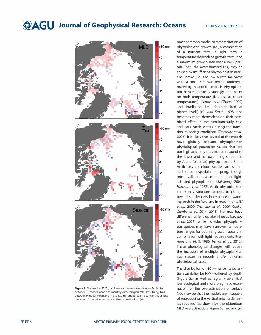
Our study also showed that simulations of surface NO3 (nutrient) and Zeu (light) associated with MLD (con-trolling the depth horizon where phytoplankton cells are) exhibited low model skill in most of the regions(Table 4) being lowest in the interior of the Arctic Ocean This observation is not necessarily new [Popovaet al 2012 Vancoppenolle et al 2013] but one should be cautious when interpreting this result becausethese three simulated parameters were positively biased (ie means usually overestimated) (Figures 8 and9) For example the simulated mean surface NO3 was vastly overestimated especially in the low-productivity nutrient-depleted interior regions of the Arctic Ocean ie the Beaufort Sea and the centralArctic Basin where model and in situ iNPP agreed best (Figures 6b and 6e Table 4) At least on a regionalscale the overestimation of surface NO3 possibly stems from spurious vertical mixing between the uppermixed layer and deeper water in the model simulations resulting in excessive nutrient supply into the sur-face layer For example except in the Greenland and Barents Seas MLD mean and variability were poorlyestimated (Table 4) and mostly overestimated (Figure 9a) by as much as twofold possibly resulting inhigher nutrients at the surface Alternatively a physiological perspective may be examined based on the
Figure 8 Same as Fig 6 but for NO3 (mmol m23) in the surface layer (0ndash10 m)
Journal of Geophysical Research Oceans 1010022016JC011993
LEE ET AL ARCTIC PRIMARY PRODUCTIVITY ROUND ROBIN 17
most common model parameterization ofphytoplankton growth (ie a combinationof a nutrient term a light term atemperature-dependent growth term anda maximum growth rate over a daily peri-od) Then the overestimated NO3 may becaused by insufficient phytoplankton nutri-ent uptake (ie too low a rate for Arcticwaters) since NPP was overall underesti-mated by most of the models Phytoplank-ton nitrate uptake is strongly dependenton both temperature (ie less at coldertemperatures) [Lomas and Glibert 1999]and irradiance (ie photoinhibited athigher levels) [Hu and Smith 1998] andbecomes more dependent on their com-bined effect in the simultaneously coldand dark Arctic waters during the transi-tion to spring conditions [Tremblay et al2006] It is likely that several of the modelshave globally relevant phytoplanktonphysiological parameter values that aretoo high and may thus not correspond tothe lower and narrower ranges requiredby Arctic (or polar) phytoplankton SomeArctic phytoplankton species are shade-acclimated especially in spring thoughmost available data are for summer light-adjusted phytoplankton [Sakshaug 2004Harrison et al 1982] Arctic phytoplanktoncommunity structure appears to changetoward smaller cells in response to warm-ing both in the field and in experiments [Liet al 2009 Tremblay et al 2009 Coello-Camba et al 2014 2015] that may havedifferent nutrient uptake kinetics [Lovejoyet al 2007] while individual phytoplank-ton species may have narrower tempera-ture ranges for optimal growth usually incombination with light requirements [Har-rison and Platt 1986 Vernet et al 2012]These phenological changes will requirethe inclusion of multiple phytoplanktonsize classes in models andor differentphysiological rates
The distribution of NO3mdashhence its poten-tial availability for NPPmdashdiffered by depth(Figure 5c) as well as region (Table 4) Aless ecological and more pragmatic expla-nation for the overestimation of surfaceNO3 may be that the models are incapableof reproducing the vertical mixing dynam-ics required (as shown by the ubiquitousMLD overestimation Figure 9a) no evident
Figure 9 Modeled MLD Zeu and sea ice concentration bias (a) MLD biasbetween 15 model mean and monthly climatological MLD (m) (b) Zeu biasbetween 9 model mean and in situ Zeu (m) and (c) sea ice concentration biasbetween 19 model mean and satellite-derived values ()
Journal of Geophysical Research Oceans 1010022016JC011993
LEE ET AL ARCTIC PRIMARY PRODUCTIVITY ROUND ROBIN 18
relationship was found between vertical resolution and skill in surface NO3 among the participating models(not shown) Indeed the future Arctic Ocean may produce less NPP per unit area due to less surface NO3 [egVancoppenolle et al 2013] resulting from enhanced freshening [Coupel et al 2015] as also hypothesized byMcLaughlin and Carmack [2010] Unlike surface NO3 deep NO3 was more realistically reproduced pan-Arcticwide in terms of the multimodel ensemble mean values at 100 km grid scales (average symbols in Figure 7)Indeed deep NO3 and sea ice concentration (ie measured as ME) were relatively well explained by the multi-model ensemble in at least four regions (Table 4) Still deep NO3 (50ndash100 m) was relatively poorly estimatedin the inflow Barents and Chukchi Seas in terms of correlation coefficients (Figures 7c and 7g) and regionalmeans (WS in Table 4) Those two regions are strongly influenced by horizontal advection of sub-Arctic inflowwaters which contribute to the nutrient supply into the Arctic Ocean via the Bering Strait and Fram StraitBarents Sea openings [eg Carmack and Wassmann 2006 Wassmann et al 2015] Torres-Valde et al [2013]estimated the volume and NO3 transports into the Arctic Ocean based on a combination of modeled and insitu velocity fields and nutrient sections total volume and NO3 transport into the Arctic Ocean at depth corre-sponded to 20 and 80 through the Bering Strait and the Barents Sea opening respectively (ie a signifi-cant contribution) Smith et al [2011] also showed the greater relative importance of this advective nutrientinput compared to vertical mixing in the Arctic Ocean
Involvement of a light-driven component of the simulation of NPP is provided by the fact that Zeu was gen-erally overestimated in all Arctic regions by most of the nine models that provided this field (Figure 9b) Thesimulated Zeu (9 model mean of 56 m) compared to the mean in situ Zeu (37 m) was deeper than MLD (18model mean of 23 m and climatological mean of 16 m) Possible explanations for the Zeu overestimationmay include the prescription of lower turbidity levels than the typical values in the Arctic Ocean In addition(or instead) the parametrization of light extinction in the water column may be associated with sea ice con-ditions ie the Zeu overestimation coupled with underestimation of sea ice concentration may result inlight being able to penetrate deeper into the water column during a simulation From a biophysical per-spective the self-shading effect caused by the presence of phytoplankton is considered in many of the par-ticipating models already Although we focused on model skill in estimating NPP not phytoplanktonbiomass the self-shading effect has been reported as negligible for high latitudes in sensitivity analyses[Manizza et al 2005] Yet other biogeochemical species like colored dissolved organic matter that couldreduce the light penetration into the water column are not represented in the models used in this study[Granskog et al 2012 Dutkiewicz et al 2015 Kim et al 2015] Nonetheless NPP was still underestimateddespite apparent light availability emphasizing a physiological coupling between light availability and lightrequirements by phytoplankton alternatively it suggests that low NPP would generate low phytoplanktonbiomass which would result in a deeper Zeu simply due to lack of light absorption
Given that the models overestimated surface NO3 and Zeu the simulated phytoplankton populations wouldexperience more nutrient and light availability which should have led to higher iNPP However the simulat-ed NPP was mostly underestimated in all regions of the Arctic Ocean clearly indicating that surfacenutrients were not the primary limiting factor for the underestimated iNPP in these model simulationsBecause the regions with higher model skill at estimating iNPP coincided with better model skill in Zeu andsea ice concentration especially in low production regions the amount of shortwave radiation or PAR trans-mitted through sea ice could account partly for underestimating iNPP [Babin et al 2015] Our findings fur-ther suggest that biological processes (ie phytoplankton growth and photosynthesis) were possiblymisrepresented by the model configurations run for this Arctic Ocean exercise A previous model intercom-parison study for lower latitudes pointed out that an improved understanding of the temperature effect onphotosynthesis and a better parameterization of the maximum photosynthetic rate are required [Carr et al2006] Hence one might argue that phytoplankton growth functions were not adequately parameterizedespecially for colder high latitudes in many models resulting in lesser utilization of surface nutrients This isdebatable in the Beaufort Sea where the effect of temperature on photosynthetic parameters over the insitu range observed (22 to 88C) was found not significant [Huot et al 2013] Furthermore a large variabilityin photosynthetic parameters and half-saturation constants exists in Arctic ecosystem models as recentlyreviewed by Babin et al [2015] during a model sensitivity exercise they showed that temperature was notas strong a limiting factor for phytoplankton growth as others (ie light and nitrate) Although it could bethat nutrients light and temperature relationships need to be adjusted to improve model skill in the ArcticOcean such a regional tuning is however not possible for global BOGCMs and ESMs
Journal of Geophysical Research Oceans 1010022016JC011993
LEE ET AL ARCTIC PRIMARY PRODUCTIVITY ROUND ROBIN 19
Simulated NPP may be low due to not only limiting factors but also because of too little biomass egthrough excessive loss of carbon from or in the upper water column Vertical export of organic matter isparameterized in all models The organic carbon to organic nitrogen stoichiometric ratio in sinking particu-late matter has been shown not to be constant in Arctic waters [Tamelander et al 2013 Michel et al 2006]as assumed in most models Arctic phytoplankton are also known to have large exudation levels during cer-tain phases of their growth cycle [Vernet et al 1998 Laroche et al 1999] which promotes the formation ofsinking aggregates resulting in significant carbon export from the surface layer when large phytoplanktoncells dominate [Reigstad et al 2011 Wassmann et al 2006] Changes in phytoplankton species compositionand bloom phenology in Arctic waters are also being reported These changes include shifts toward smallercells possibly with different physiology especially in the freshening Beaufort Sea and Canadian Arctic Archi-pelago [Li et al 2009 Tremblay et al 2009] which will again affect vertical export fluxes Changes in bloomphenology have been described as lengthening bloom periods or even the presence of fall blooms(reviewed by Babin et al [2015] Michel et al [2006 2015]) However these changes are fairly recent and like-ly not yet simulated by models nor captured by the in situ data used for our exercise despite covering fivedecades back (ie diminishing the likelihood of an effect in our field data set)
If bottom-up factors were not the main or sole controls on phytoplankton productivity grazing could benot only may grazers reduce NPP but they also regulate vertical flux If simulated grazing rates were toohigh then the resulting nutrient concentrations would be much higher than the values of the high satura-tion constants used This scenario was ruled out for high latitudes by a PISCES-based model simulation inwhich bottom-up controls did dominate [Aumont et al 2015] On the other hand the northward advectiveinflow of sub-Arctic water has been reported to also carry significant zooplankton biomass [Wassmannet al 2015] Hence it is possible that the Arctic Ocean primary production in model simulations might bereduced under increased grazing pressure from such sub-Arctic (expatriate) zooplankton Such a hypotheti-cal extension of sub-Arctic grazing influence to the interior regions of the Arctic Ocean is not currently sup-ported by observations [Kosobokova and Hopcroft 2010] Much is changing with respect to trophicstructure in the Arctic Ocean including grazer community composition and biodiversity [Bluhm et al 2015]all of which may or may not be simulated by the models with consequences for estimating iNPP Howeverwe currently lack a comprehensive review and climatology for in situ micro meso and macrozooplanktongrowth and grazing rates in the Arctic Ocean to broadly assess model relative skill
Our use of an in situ NPP database allowed the assessment of model skill in ice-influenced as well as in ice-free waters overcoming a limitation encountered by previous model intercomparison exercises for the Arc-tic Ocean [eg Popova et al 2012 Vancopenolle et al 2013] that depended on satellite-derived NPP whichis not available for ice-covered regions Regardless of whether sea ice was present or not the mean and var-iance of in situ iNPP were almost identical confirming that the ice-influenced regions could be as produc-tive as the ice-free regions (Table 2) It should be noted that the similarity could be due to biased seasonalcoverage by field studies in ice-free waters introducing more measurements collected in late summer andfall (ie September) thus lowering the ice-free iNPP average (not shown) Alternatively the similarity in sim-ulated iNPP values in ice-free and ice-influenced areas could result from the averaging of regional differ-ences previously observed in field and satellite-derived NPP data [eg Arrigo et al 2012 Hill et al 2013Ardyna et al 2013] as well as in model simulations [eg Zhang et al 2015] Recently Jin et al [2016]showed that simulated under-ice production is also regionally different (ie higher in the Arctic shelvespossibly due to enhanced nutrient supply) [Zhang et al 2015] but not necessarily related to the recentdecrease in sea ice concentration especially in marginal ice zones Regardless of whether NPP was mea-sured in deep versus shallow areas or ice-influenced versus open water regions model skill for iNPP differedlittle on such spatial scales
Time did make a difference however Model skill varied from decade to decade and higher model skill wasfound for the most recent decade (Figures 4e and 4f) when in situ iNPP and NO3 were lower (Table 2) sincethe models performed better with low iNPP For example on a pan-Arctic scale in situ carbon uptake ratesdecreased to 177 mg C m22 d21 (N 5 344 2000ndash2011) compared to 316 mg C m22 d21 in the earlier deca-des (N 5 391 1959ndash1989) Similarly in situ depth-averaged NO3 decreased from 51 mmol m23 (N 5 2841979ndash1999) to 29 mmol m23 (N 5 379 2000ndash2011) These decreases likely resulted from differences in geo-graphical sampling distribution between decades (Figure 1) For example during 2000ndash2011 more datawere available from the large Canadian and International Polar Year programs in low production regions
Journal of Geophysical Research Oceans 1010022016JC011993
LEE ET AL ARCTIC PRIMARY PRODUCTIVITY ROUND ROBIN 20
such as the Beaufort Sea and the central Arctic Basin (Figure 1c) Not all of the participating models cap-tured these decreasing changes in simulated iNPP and NO3 (not shown) However regardless of whethermodel iNPP estimates increased or decreased over the most recent decade simulated iNPP values becamemore comparable to in situ values on a pan-Arctic scale such that model skill was seen to be improved inmore recent years (Figures 4e and 4f) On a seasonal time-scale the models generally performed poorly inthe beginning of the growing season (AprilndashJune) compared to later months (Figures 4g and 4h) For somemodels this could be due to insufficient penetration of winter mixing as the main mechanism controllingbasin-scale patterns of nutrient supply [eg Popova et al 2012] though as stated earlier MLD was overesti-mated overall (Figure 9a) Also occurring at this time is the critical balance between the onset and phenolo-gy of sea ice melting ice algal bloom andor phytoplankton bloom small mismatches in timing amongthem resulted in a large variability of simulated phytoplankton availability especially at the Arctic marginalseas [Ji et al 2013]
Model quantification of biogeochemical processes is highly dependent on how accurately physical fieldsare simulated [Friedrichs et al 2006 Popova et al 2012] Submesoscale physical features are especiallyimportant to biogeochemical processes affecting the horizontal and vertical distribution of nutrients andphytoplankton biomass [Watanabe et al 2014] Most of the participating models are developed on globalscales and only four of them are regional models of the order of 10 km resolution (Table 1) The Rossby radi-us of deformation is dramatically reduced with increasing latitude and it becomes less than 10 km in theArctic Ocean Hence those models with resolution of the order of 10ndash100 km may not adequately resolvesubmesoscale physical features at the surface layer that are likely critical for Arctic biogeochemical process-esmdashin particularmdashregionally [Timmermans et al 2012] rather than larger-scale physical processes deter-mining the response of the pan-Arctic marine ecosystem High spatial resolution models or more Arctic-appropriate parameterizations and closures are necessary to capture small-scale physical processes such aseddies tides fronts internal waves as well as interactions between shelf and open ocean or sea and ice pro-cesses that can influence phytoplankton growth especially in high-productivity coastal shelf regions adja-cent to sub-Arctic waters Indeed regionally model skill patterns are contradictory such that the GreenlandSea has a very closely simulated surface and deep NO3 and MLD (Table 4) but the least skill in simulated seaice concentration (Figure 9c) yet it has the lowest skill in iNPP underestimating it (Figure 6f) Converselythe Beaufort Sea shows medium skill in deep NO3 least skill in surface NO3 (overestimating concentrations)and yet the best skill in iNPP (Table 4)mdashstill underestimating iNPP and its variability (Figure 6b) though lessthan other Arctic Ocean subregions Assuming improved parameterization of nutrient light and tempera-ture relationships of phytoplankton growth a higher spatial resolution model could potentially produce sig-nificant subregional features [eg Yool et al 2015] as mesoscale and submesoscale processes have beenshown to stimulate biological productivity in lower latitudes [McGillicuddy et al 1998 Oschlies and Garcon1998 Levy et al 2001] Finally coastal regions characterized by elevated primary productivity are also notproperly resolved by a coarse model grid in general [Aumont et al 2015] Higher resolution in ecosystemcomplexity has already been shown to lead to improved realism of BOGCM high latitude simulations withthe addition of slow growing macrozooplankton leading to the successful representation of the differentbloom dynamics in the Southern Ocean [Le Quere et al 2016] Much effort is now being applied in themodeling community to introduce high-resolution strategies into BOGCMs especially those regionallyfocused on the Arctic Ocean [Interagency Arctic Research Policy Committee 2013] with the hope that repro-ducing meso and submesoscale processes and features will improve their predictive skill for iNPP and otherbiogeochemical properties in the Arctic Ocean
6 Summary and Recommendation
Using in situ satellite-derived and climatological data we have analyzed model estimates of iNPP and NO3
associated with physical variables such as MLD Zeu and sea ice concentration from 21 BOGCMs and ESMsduring the period of 1959ndash2011 although the time span of simulation as well as the initialization and forc-ing were different among the participating models No models fully reproduced the variability of in situmeasurements whereas some of them exhibited almost no bias Generally the models captured the spatialfeatures of the iNPP distribution lower iNPP in the interior regions and higher iNPP in the inflow regionsThe models exhibited different regional characteristics in estimating iNPP since each modelrsquos skill was afunction of environmental factors with distinctive sensitivity in one region versus another For example
Journal of Geophysical Research Oceans 1010022016JC011993
LEE ET AL ARCTIC PRIMARY PRODUCTIVITY ROUND ROBIN 21
MLD and NO3 were reproduced well in the Atlantic-side inflow and outflow regions Zeu had greater skill inthe interior regions and sea ice concentration was reasonably well estimated everywhere except in theGreenland Sea Most of the models generally underestimated mean iNPP in spite of overestimating Zeu andsurface NO3 especially in the Chukchi and Greenland Seas where mean in situ iNPP is high Regionallymodel iNPP was best estimated in the regions where simulated surface NO3 was most overestimated rela-tive to in situ values and where both sea ice concentration and Zeu were reproduced well such as the Beau-fort Sea and the central Arctic Basin By contrast iNPP exhibited the largest model-data disagreement in theGreenland Sea where the simulated surface NO3 and MLD had greater model skill but sea ice concentrationhad lower model skill
The Arctic Ocean appears to be experiencing a fundamental shift from a polar to a temperate mode whichis likely to alter its marine ecosystem [Yool et al 2015 Wassmann et al 2015] Under a changing climatesea ice loss shifts in composition and distribution of phytoplankton functional types and bloom phenologychanges already play a role in the Arctic Ocean marine ecosystem [eg Li et al 2009 Ardyna et al 2014]Globally changes in nutrient and light availability have emerged as the most important determinants inmodels for alterations in simulated growth rates with light generally playing a lesser role except for thevery high latitudes particularly the Arctic Ocean [Laufkeurootter et al 2015] At these high latitudes tempera-ture does not appear to play a physiological role but could well play an ecological role of controlling phyto-plankton bloom composition and phenology [Babin et al 2015] Thus ecosystem processes and algalphysiology in models need to be carefully parameterized for the Arctic Ocean in order to better quantifyuncertainties in estimating primary production including under-ice primary production and ice algae pro-duction [Leu et al 2015 Jin et al 2016] enhanced functional types for all levels of the marine food web[Babin et al 2015] and the role of horizontal advection of planktonic organisms versus their vertical export[Wassmann et al 2015] Furthermore it is necessary to resolve submesoscale physical processes to decidethe apparently contradictory bottom-up controls of NPP and the resulting biogeochemical cycles in the var-ious subregions of the Arctic Ocean with the hope that BOGCMs and ESMs perform within the uncertaintydue to natural variability Last but not least models will continue to improve their skill when additional vali-dating data sets and climatologies are gathered and openly shared for relevant biogeochemical physiologi-cal and ecological variables in the Arctic Ocean
Appendix A Brief Description of Participating Models
A1 Model 1HYCOM-NORWECOM [Samuelsen et al 2015] is a regional coupled physical-biogeochemical model with 11compartments in the biogeochemical model The physical model is the Hybrid Coordinate Ocean Model(HYCOM) [Bleck 2002] adapted to the North Atlantic and Arctic Ocean [Bertino and Lisaeter 2008] The mod-el encompasses the entire North Atlantic and has open lateral boundaries at the Bering Strait in the PacificOcean and near the equator between 38S and 168S in the Atlantic Ocean the model is relaxed toward clima-tological values at the lateral boundaries The model is forced by ERA-Interim [Dee et al 2011] hydrologicalforcing from TRIP [Oki and Sud 1998] but does not include tidal forcing The sea ice model uses an elastic-viscous-plastic (EVP) rheology [Hunke and Dukowicz 1997] while thermodynamics are described in Drangeand Simonsen [1996] NORWEgian ECOlogical Model (NORWECOM) [Aksnes et al 1995 Skogen and Soslashiland1998] is coupled online to HYCOM and uses HYCOM facility for advection of tracers and has the same time-step as the physical model The current model version includes two classes of phytoplankton (diatom andflagellates) two classes of zooplankton (meso and microzooplankton) derived with the same formulationfrom the model ECOHAM4 [Peuroatsch et al 2009] three types of nutrients (N P and Si) and detritus (N and P)biogenic Si and oxygen (O2) Additionally riverine nutrient loads are based on the results from the Global-NEWS model [Seitzinger et al 2005] The model assumes a constant element ratio (ie Redfield) as well asconstant chlorophyllN ratio in phytoplankton In the model light does not propagate through sea icetherefore the model is not expected to yield realistic primary production and nutrients in areas with thinice cover where light actually is available for primary production
A2 Model 2This global biogeochemical model (1998ndash2014) uses the PISCES formulation on the horizontal curvilineargrid ORCA025 and 75 vertical levels It is forced offline by daily fields of an ocean circulation simulation
Journal of Geophysical Research Oceans 1010022016JC011993
LEE ET AL ARCTIC PRIMARY PRODUCTIVITY ROUND ROBIN 22
Nucleus for European Modelling of the Ocean (NEMO)-Ocean PArallelise (OPA) (version 31) [Madec 2008]Atmospheric forcings are 3 hourly ERA-Interim reanalysis product with the CORE bulk formulation There isno assimilation of physical data The sea ice model is the Louvain la Neuve sea Ice Model version 2 (LIM2)with EVP rheology [Fichefet and Morales Maqueda 1997] PISCES (volume 2) [Aumont et al 2015] is a modelof intermediate complexity designed for global ocean applications and is a component of the NEMO model-ing system It has 24 prognostic variables and simulates biogeochemical cycles of O2 C and the mainnutrients controlling phytoplankton growth (NO3 ammonium (NH4) phosphate (PO4) silicate (SiO4) andFe) The model distinguishes four plankton functional types based on size two phytoplankton groups(nanophytoplankton and diatoms) and two zooplankton groups (micro and mesozooplankton) PISCEStraces three nonliving pools for small and big particulate organic carbon (POC) and semilabile dissolvedorganic carbon (DOC) Version 35 of NEMO-PISCES with default parameter set is used here The configura-tion is described and assessed in the Product User Manual and Quality Information Document (httpmarinecopernicuseudocumentsPUMCMEMS-GLO-PUM-001-018pdf and httpmarinecopernicuseudocumentsQUIDCMEMS-GLO-QUID-001-018pdf) Daily and monthly mean outputs are available on Coper-nicus Marine Service website (httpmarinecopernicuseu)
A3 Model 3This model is the Plankton Types Ocean Model 53 (PlankTOM53) biogeochemical model coupled to theNEMO (version 23) global ocean circulation model and sea ice model (LIM2) The biological model is a 26component marine pelagic ecosystem model including three phytoplankton components (diatoms cocco-lithophores and mixed phytoplankton) two zooplankton components (micro and mesozooplankton) DOCsmall and large detrital POC and particulate organic Fe detrital particulate Si and calcite and dissolved NO3SiO4 and Fe [Buitenhuis et al 2013] Each phytoplankton functional type has C chlorophyll and Fe compo-nents linked with a dynamic photosynthesis model [Buitenhuis and Geider 2010] The standard simulationwas spun up from 1920 to 1955 and for the purpose of this paper the optimized simulation was run from1956 to 2013 [Buitenhuis et al 2013]
A4 Model 4This model is the Plankton Types Ocean Model 10 (PlankTOM10) biogeochemical model coupled to theNEMO (version 31)-LIM2 ocean circulation and sea ice model The biological model is a 37 componentmarine pelagic ecosystem model including six phytoplankton components (diatoms coccolithophorespicophytoplankton N2-fixers phaeocystis and mixed phytoplankton) three zooplankton components(micro meso and macrozooplankton) bacteria DOC small and large detrital POC and particulate organicFe detrital particulate Si and calcite and dissolved NO3 SiO4 and Fe [Le Quere et al 2016] PlankTOM10 hasthe same dynamic photosynthesis model as PlankTOM53 (Model 3) In addition it has an improved repre-sentation of the difference between the high latitude Northern and Southern Hemisphere phytoplanktonblooms through the representation of slow growing macrozooplankton The different physical settingsresult in different overwintering macrozooplankton populations in turn leading to different trophic cas-cades and more realistic phytoplankton blooms [Le Quere et al 2016]
A5 Model 5The Carbon Ocean Biogeochemistry and Lower Trophics (COBALT) version 10 marine ecosystem modeluses 33 state variables to resolve global-scale cycles of C N P Si Fe calcium carbonate (CaCO3) O2 andlithogenic material [Stock et al 2014a] COBALT derives many elements of its biogeochemical formulationfrom the TOPAZ model (see Model 6) However COBALT enhances the resolution of planktonic food webdynamics to better understand the climate impacts on the flow of energy from phytoplankton to fish [Stocket al 2014b] The model includes three phytoplankton groups (small large and diazotrophs) and uses thevariable chlorophyllC formulation of Geider et al [1997] to estimate NPP Results contributed to this studywere conducted with the Modular Ocean Model (MOM) version 4p1 [Griffies 2012] with sea ice dynamics asdescribed in Winton [2000] The model was run on a global domain with a nominal spatial resolution of 18
and a tripolar Arctic grid The model uses 50 vertical layers with a nominal resolution of 10 m over the top200 m Simulations are forced with the Coordinated Ocean-ice Reference Experiment version 2 (CORE2)data set [Large and Yeager 2009] The 60 year forcing period was looped twice and results from the secondloop provided for this study Surface salinity is relaxed to observations with 2 month relaxation time-scale inorder to avoid salinity drifts characteristic of long integrations of ocean-ice simulations without fully
Journal of Geophysical Research Oceans 1010022016JC011993
LEE ET AL ARCTIC PRIMARY PRODUCTIVITY ROUND ROBIN 23
coupled atmosphere dynamics [Griffies et al 2009] Complete details of the simulation and model validationcan be found in Stock et al [2014a]
A6 Model 6Tracers of Ocean Phytoplankton with Allometric Zooplankton version 20 (TOPAZ2) is an ocean biogeo-chemical and ecological model developed at NOAArsquos Geophysical Fluid Dynamics Laboratory for globalEarth System Model simulations contributed to the 5th assessment report of the Intergovernmental Panelon Climate Change [Dunne et al 2012b2013] TOPAZ2 includes 30 tracers to describe the cycles of C NP Si Fe O2 alkalinity and lithogenic material as well as surface sediment calcite dynamics [Dunne et al2012a] TOPAZ2 considers three explicit phytoplankton groups (small large and diazotrophs) that utilizea modified growth physiology after Geider et al [1997] with Eppley [1972] temperature functionality andiron colimitation with luxury uptake after Sunda and Huntsman [1997] CO2NO3O2 stoichiometry is10616150 after Anderson [1995] NP is based on optimal allocation after Klausmeier et al [2004] Com-plete technical details are available in the supplementary information of Dunne et al [2013] Results con-tributed to this study were conducted with the MOM (version 4p1) [Griffies 2012] with sea ice dynamicsas described in Winton [2000] The model was run on a global domain with a nominal spatial resolution of18 and a tripolar Arctic grid The model uses 50 vertical layers with a nominal resolution of 10 m over thetop 200 m Simulations are forced with the CORE2 data set [Large and Yeager 2009] The 60 year forcingperiod was looped twice and results from the second loop provided for this study Surface salinity isrelaxed to observations with 2 month relaxation time-scale in order to avoid salinity drifts characteristicof long integrations of ocean-ice simulations without fully coupled atmosphere dynamics [Griffies et al2009]
A7 Model 7SINMOD is a model system that has been continuously developed over 30 years and includes a hydrody-namic and a sea ice module [Slagstad and McClimans 2005] an ecosystem module [Wassmann et al 2006]and stage resolved zooplankton models [Slagstad and Tande 2007] The hydrodynamic model is based onthe primitive Navier-Stokes equations and is established on a Z-grid [Slagstad and McClimans 2005] The icemodel is similar to that of Hibler [1979] and has two state variables ice thickness and ice concentration Theice momentum equation is solved together with an equation for the ice internal stress using the EVPdynamical model of Hunke and Dukowicz [1997] The ecosystem model includes nutrients (NO3 NH4 andSiO4) phytoplankton (diatoms and flagellates) bacteria heterotrophic nanoflagellates microzooplanktonand two mesozooplankters the Atlantic Calanus finmarchicus and the arctic C glacialis two compartmentsfor fast and slow sinking detritus DOC and sediments The model uses constant stoichiometry with a CNratio equal 76 based upon average data from the Barents Sea [Reigstad et al 2002] In the present studySINMOD data are from a pan-Arctic configuration with 20 km horizontal grid resolution and with 25 verticallayers Forcing fields includes atmospheric forcing from the ERA-Interim reanalysis (httpwwwecmwfint)[Dee et al 2011] tides from TPXO 62 model prescribed at open boundaries and freshwater run-off fromR-ArcticNet (httpwwwr-arcticnetsrunhedu) More details of the recent updates of SINMOD and themodel setup may be found in Slagstad et al [2015]
A8 Model 8The NorESM-OC is the ocean component of the Norwegian Earth System Model (NorESM) It is a coupledBOGCM which comprises the Miami Isopycnic Coordinate Ocean Model (MICOM) coupled with the Ham-burg Oceanic Carbon Cycle (HAMOCC)25 model [Schwinger et al 2016] HAMOCC consist of a Nutrient-Phytoplankton-Detritus-Zooplankton (NPDZ)-type ecosystem model where the primary production isformulated as a function of phytoplankton growth and nutrient concentration within the euphotic layer(fixed at 100 m) In addition to multinutrients (ie NO3 PO4 and dissolved Fe) colimitation the phyto-plankton growth is regulated by light availability and temperature The model adopts a generic singleclass phytoplankton and zooplankton compartment The particulate materials (ie POC biogenic opaland CaCO3) produced at the surface sink with constant velocities and are remineralized at depth The pro-duction of surface opal and CaCO3 is determined by the SiO4 availability at the surface Nonremineralizedparticles reaching the seafloor undergo chemical reactions with sediment pore waters bioturbation andvertical advection within the sediment module For the simulation produced in this study the NorESM-OCwas forced by the CORE2 atmospheric reanalysis data
Journal of Geophysical Research Oceans 1010022016JC011993
LEE ET AL ARCTIC PRIMARY PRODUCTIVITY ROUND ROBIN 24
A9 Model 9This model is the BiologyIceOcean Modeling and Assimilation System (BIOMAS) a coupled biophysicalmodel [Zhang et al 2010a] with four model elements an ocean circulation model a sea ice model a pelag-ic biological model and a sea ice algae model The ocean circulation model is based on the Parallel OceanProgram (POP) developed at Los Alamos National Laboratory [Smith et al 1992] and modified by Zhangand Steele [2007] so that open boundary conditions can be specified The POP ocean model is further modi-fied by Zhang et al [2010b] to incorporate tidal forcing from eight primary constituents [Gill 1982] The seaice model is a thickness and enthalpy distribution (TED) sea ice model [Zhang and Rothrock 2003 Hibler1980] with eight categories each for ice thickness ice enthalpy and snow depth It is adopted from thePan-arctic IceOcean Modeling and Assimilation System (PIOMAS) [Zhang and Rothrock 2003] and capableof assimilating satellite observations of sea ice concentration [Lindsay and Zhang 2006] and sea surfacetemperature [Manda et al 2005 Schweiger et al 2011] The pelagic biological model is an 11 componentmarine pelagic ecosystem model including two phytoplankton components (diatoms and flagellates) threezooplankton components (microzooplankton copepods and predatory zooplankton) dissolved organicnitrogen (DON) detrital particulate organic nitrogen (PON) particulate organic Si NO3 NH4 and SiO4 (seeFigure 3 in Zhang et al [2014] also see Kishi et al [2007]) Values for key biological parameters used in themodel are listed in Zhang et al [2010a] The sea ice algal component of BIOMAS represents colonies in a2 cm layer at the bottom of each of eight sea ice thickness categories coupled to the pelagic modelthrough nutrient and biotic fluxes The sea ice algae model has two ice algae components (diatoms andflagellates) with NO3 NH4 and SiO4 as limiting nutrients for ice algal growth Nutrient and biotic exchangeat the sea ice and water interface is based on Jin et al [2006]
A10 Model 10This model is NEMO (version 32)-MEDUSA a coupled biophysics model comprised of an ocean general cir-culation model (OGCM) a sea ice model and a representation of marine biogeochemistry [Popova et al2010 2012] Ocean circulation is modeled using OPA version 9 (OPA9) [Madec 2008] a primitive equationmodel configured at global-scale with a horizontal resolution of approximately 0258 and 64 grid levels inthe vertical [Popova et al 2010] The model grid is tripolar with cell sizes ranging approximately 68ndash154 km horizontally and increasing in thickness from 6 m at the surface to approximately 250 m at abyssaldepths OPA9 includes partial level thicknesses at the seafloor to improve bottom circulation and a parame-terized turbulent kinetic energy scheme for vertical mixing [Gaspar et al 1990 Madec 2008] The model isforced at the surface using bulk formulae [Large and Yeager 2004] fed using DFS41 climatology fields ofatmospheric properties and downward heat and freshwater fluxes [DRAKKAR Group 2007] Sea ice is repre-sented with LIM2 [Timmermann et al 2005] based on a viscous-plastic ice rheology [Hibler 1979] with threelayer (two ice and one snow) thermodynamics [Semtner 1976] LIM2 is coupled to OPA9 every five oceantime steps through a nonlinear quadratic drag law of ocean-ice shear [Timmermann et al 2005] and repre-sents detailed heat and freshwater fluxes [Fichefet and Morales Maqueda 1997] OPA9 and LIM2 are com-bined as the NEMO physical model [Madec 2008] Marine biogeochemistry is represented using the Modelof Ecosystem Dynamics nutrient Utilization Sequestration and Acidification (MEDUSA) [Yool et al 2011]This includes the N Si and Fe cycles in a model of the pelagic ecosystem that resolves nanophytoplanktondiatoms and micro and mesozooplankton as well as size-resolved (small and large) detrital material includ-ing biomineral ballasting [Armstrong et al 2002] MEDUSA has simplified seafloor remineralization of organ-ic material and does not explicitly include sea ice algae
A11 Model 11 and 12NEMO (version 32)-European Regional Seas Ecosystem Model (ERSEM) is a global ocean model thatincludes the NEMO ocean circulation model the ERSEM marine biogeochemistry model and the Los Ala-mos sea ice model (CICE) NEMO (version 32) is a framework of ocean related engines ocean dynamicsthermodynamics sinks and sources and transport [Madec 2008] The CICE model [Hunke et al 2013] hasseveral interacting components a thermodynamic submodel an ice dynamics submodel a vertical and ahorizontal transport submodel ERSEM is a lower trophic level biogeochemical cycling carbon-based pro-cess model that uses the functional-group approach [Blackford et al 2004 Butenscheuroon et al 2016] The C NP Si and Fe cycles are explicitly resolved with variable stoichiometry The pelagic ERSEM model simulatesfour phytoplankton functional types three zooplankton functional types one bacterial functional type andsix detritus size classes The benthic ERSEM is a simple parameterization of remineralization where
Journal of Geophysical Research Oceans 1010022016JC011993
LEE ET AL ARCTIC PRIMARY PRODUCTIVITY ROUND ROBIN 25
sedimented organic matter is recycled to the water column in inorganic form The simulations were run aspart of the iMarNet project an intercomparison project of six UK biogeochemical models [Kwiatkowski et al2014] The simulation of Model 12 (xhonc) uses an updated configuration of the ERSEM model with a newiron model updated food web and reduced detrital sinking rate relative to the simulation of Model 11(xhonp)
A12 Model 13PELAgic biogeochemistry for Global Ocean Simulations (PELAGOS) [Vichi et al 2007a2007b] is a globalocean biogeochemical model that consists of the coupling between the NEMO (version 34) [Madec 2008]and the Biogeochemical Flux Model (BFM version 51 httpbfm-communityeu) [Vichi et al 2015a] Theocean model is computed on the ORCA2 grid that has a nominal resolution of 28 with a refinement of thelatitudinal grid size toward the equator down to 058 with 30 vertical levels and partial step parameteriza-tion to increase the resolution of bottom gradients The physical parameterizations are as in Vichi et al[2007b] The sea ice model is LIM2 and the BFM model can directly be coupled with NEMO [Vichi et al2015b] The BFM is based on a biomass continuum description of the lower trophic levels of the marine sys-tem [Vichi et al 2015b] The model implements a set of biomass-based differential equations that solve thefluxes of C N P Si and Fe among selected biological functional groups representing the major componentsof the lower trophic levels The functional groups in the pelagic environment are represented by unicellularplanktonic autotrophs (pico and nanophytoplankton and diatoms) zooplankton (nano micro and meso-zooplankton) and heterotrophic oxic and anoxic bacterioplankton The model also simulates the dynamicsof NO3 NH4 PO4 biogenic Si Fe O2 and it has an explicit parameterization of the biochemical cycling ofdissolvedparticulate nonliving organic matter Another peculiarity of the model is that the nutrient stoichi-ometry is not fixed and therefore the ratios of C to N P and Si can vary within the living functional groupsas well as the chlorophyllC ratio in phytoplankton This simulation includes nutrient river inputs from Cotrimda Cunha et al [2007] but no benthic remineralization
A13 Model 14A marine biogeochemical (mBGC) module [Moore et al 2004 Jin et al 2012 2016] is incorporated in a glob-al version of the POP-CICE model developed at Los Alamos National Laboratory A subgrid-scale ocean mix-ing scheme [Jin et al 2012] was added to reduce model errors in simulated mixed layer depth salinity andnutrients in the Arctic Ocean The pelagic component of mBGC includes 26 state variables of multiplenutrients phytoplankton zooplankton and detritus The ice algal component of mBGC represents coloniesin a 3 cm layer at the bottom of each sea ice thickness category coupled to the pelagic model throughnutrient and biotic fluxes This submodel was based on biophysical ice core data collected in land-fast iceoffshore from Barrow Alaska [Jin et al 2006] and coupled with a pelagic ecosystem model in vertically 1-Dmodels [Jin et al 2007] and global POP-CICE model settings [Deal et al 2011 Jin et al 2012 2016]
A14 Model 15This model is based on the ocean circulation model OPA the dynamical component of NEMO (version 35)It solves the primitive equations on the Arakawa C-grid with a second-order centered finite differencescheme [Madec 2008] It assumes the Boussinesq and hydrostatic approximations the incompressibilityhypothesis and uses a free-surface formulation [Roullet and Madec 2000] The density is computed frompotential temperature salinity and pressure using the Jacket and Mcdougall [1995] equation of state Verti-cal mixing is computed from a turbulence closure scheme based on a prognostic vertical turbulent kineticequation which performs well in the tropics [Blanke and Delecluse 1993] Partial step formulation of bottomtopography is used instead of a full step one [Bernard et al 2006] LIM2 is a two-level thermodynamic-dynamic sea ice model in which sensible heat storage and vertical heat conduction within snow and ice aredetermined by a three-layer model (one layer for snow and two layers for ice) [Fichefet and MoralesMaqueda 1997 Bouillon et al 2009] PISCES is the biogeochemical component of NEMO and it simulatesthe lower trophic levels of marine ecosystem and the biogeochemical cycles of carbon and of the mainnutrients (P N Fe and Si) [Aumont and Bopp 2006] There are 24 prognostic variables including two phyto-plankton compartments (diatoms and nanophytoplankton) two zooplankton size-classes (micro and meso-zooplankton) and a description of the carbonate chemistry Formulations in PISCES are based on a mixedMonod-Quota formalism on one hand stoichiometry of C N and P is fixed and growth rate of phytoplank-ton is limited by the external availability in N P and Si On the other hand the Fe and Si quotas are variable
Journal of Geophysical Research Oceans 1010022016JC011993
LEE ET AL ARCTIC PRIMARY PRODUCTIVITY ROUND ROBIN 26
and growth rate of phytoplankton is limited by the internal availability in Fe There are three nonliving com-partments semilabile-dissolved organic matter small and big sinking particles
A15 Model 16This simulation is based on the global ocean biogeochemical model NEMO-PISCES NEMO (version 34) wasrun with horizontal resolution of up to 18 by 18 (globally 362 longitude 3 292 latitude grid points) and with46 vertical levels The model results are available for 2002ndash2011 For those years external ocean-surfaceforcing was specified from the CORE2 (2002ndash2007) and NCEPDOE AMIP-II Reanalysis (Reanalysis-2) data(2008ndash2011) The ocean circulation model is based on the hydrostatic primitive equation model OPA[Madec et al 1998] and is a finite difference OGCM with a free sea surface OPA uses a global tripolarorthogonal curvilinear grid to avoid singularity points inside the computational domain and attain the ratioof anisotropy of nearly one [Madec and Imbard 1996] The variables are distributed on a 3-D Arakawa-Ctype grid The sea ice model (LIM3) is a C-grid dynamic-thermodynamic model including the representationof the subgrid-scale distributions of five-category sea ice thickness enthalpy salinity and age distributionsThe representation of sea ice is done through a velocity vector and a series of ice state variables describedin Vancoppenolle et al [2009a] Brine entrapment and drainage as well as brine impact on ice thermodynam-ics and a snow ice formation scheme are explicitly included [Vancoppenolle et al 2009a 2009b] The bio-geochemical model used is PISCES (volume 2) [Aumont et al 2015] It has 24 prognostic variables andsimulates the lower trophic levels of marine ecosystems and the biogeochemical cycles of O2 C and themain nutrients (P N Fe and Si) The model distinguishes four plankton functional types based on size twophytoplankton groups (nanophytoplankton and diatoms) and two zooplankton groups (micro and meso-zooplankton) Prognostic phytoplankton variables are total biomass in C Fe Si (for diatoms) and chlorophylland hence the FeC SiC chlorophyllC ratios are fully predicted by the model For zooplankton all O C Nand P ratios are kept constant and total biomass in C is the only prognostic variable The bacterial pool isnot modeled explicitly
A16 Model 17This simulation is based on the NEMO-PISCES model The ocean component uses NEMO (version 32)[Madec 2008] in the ORCA1 configuration with horizontal resolution from 18 in polar regions to 138 nearthe equator and 42 vertical levels This configuration includes an improved Turbulent Kinetic Energy (TKE)closure scheme based on Blanke and Delecluse [1993] The ocean radiative scheme is represented by three-wave-band scheme of Lengaigne et al [2007] which accounts for influence of phytoplankton chlorophyllThe sea ice model is GELATO5 [Salas Melia 2002] which considers four ice thickness categories (0ndash03 m03ndash08 m 08ndash3 m and over 3 m) Each category has 10 vertical layers with enhanced resolution near thetop of the slab The sea ice dynamics is represented by the EVP rheology [Hunke and Dukowicz 1997] Thebiogeochemical model PISCES [Aumont and Bopp 2006] simulates the biogeochemical cycles of O2 C andthe main nutrients NO3 NH4 PO4 SiO4 Fe two sizes of phytoplankton two sizes of zooplanktonsemilabile-dissolved organic matter and small and big sinking particles Three different sources supplynutrients atmospheric dust deposition [Tegen and Fung 1995 Jickells and Spokes 2001 Moore et al 2004]rivers [Ludwig et al 1996] and sediment mobilization [Johnson et al 1999 de Baar and de Jong 2001] Themodel input of riverine-dissolved inorganic carbon (DIC) and DOC is taken from the annual estimates of theGlobal Erosion Model [Ludwig et al 1996] The DOC from rivers is assumed to be labile and is directly con-verted to DIC upon its delivery to the ocean Inputs of dissolved Fe NO3 PO4 and SiO4 are computed fromthe sum of DIC and DOC river input using a constant set of ratios for CNPSiFe as computed from Meybeck[1982] for CN from Takahashi et al [1985] for NP from de Baar and de Jong [2001] for FeC and fromTreguer et al [1995] for SiC More complete descriptions of the whole ocean-sea ice and marine biogeo-chemistry component are provided by Voldoire et al [2013] and Seferian et al [2013] respectively
A17 Model 18This model is the MIT general circulation model (MITgcm) [Marshall et al 1997] coupled with a sea ice mod-el and with a pelagic biogeochemical model The coupled model is configured on a lsquolsquocubed-spherersquorsquo gridencompassing the Arctic domain with open boundaries at around 558N in the Atlantic and Pacific sectorsPrescribed boundary conditions for potential temperature salinity flow and sea surface elevation are pro-vided from previous integrations of a global configuration of the same model [Menemenlis et al 2005] Thesea ice component follows the viscous-plastic rheology formulation of Hibler [1979] with momentum
Journal of Geophysical Research Oceans 1010022016JC011993
LEE ET AL ARCTIC PRIMARY PRODUCTIVITY ROUND ROBIN 27
equations solved implicitly on a C-grid [Arakawa and Lamb 1977] using a procedure based on Zhang andHibler [1997] The biogeochemical component improved from previous applications in Arctic waters [LeFouest et al 2011 2013] has 10 state variables [see Le Fouest et al 2015 Figure 1] Equations and biologicalparameters are listed in Le Fouest et al [2005] It includes NO3 NH4 2 size-fractionated phytoplankton andzooplankton DON PON bacteria and riverine DON (RDON) that couples the marine and terrestrial cyclingof N The RDON flux is based on the approach developed by Manizza et al [2009] using seasonally explicitregression relationships quantifying the covariation between freshwater discharge and measured RDON
A18 Model 19The NorESM is a fully coupled climate-biogeochemical model [Tjiputra et al 2013] It is the fully coupled ver-sion of Model 8 described above In this configuration the NorESM-OC is coupled with atmospheric generalcirculation (modified from Community Atmospheric Model CAM4) land (Community Land Model CLM4)and sea ice (CICE version 4) For the simulation performed in this study we apply the standard CoupledModel Intercomparison Project phase 5 (CMIP5) protocol for the historical and future high CO2 (RCP85)scenario
A19 Model 20The GISS-E2-R-CC is a coupled atmosphere-land-ocean-ice model with ocean biogeochemistry explicitlysimulated [Romanou et al 2013 2014] GISS-E2 is the GISS atmospheric model within the coupled climatemodel which was submitted in the CMIP5 [Schmidt et al 2014] and which employs a very accurate andnondiffusive quadratic upstream differencing scheme for the advection of tracers such as CO2 The GISS-E2-R ocean model [Russell et al 1995 Hansen et al 2007] is a non-Boussinesq mass-conserving ocean modelwith a free surface and natural surface boundary fluxes of freshwater and heat It uses the Gent and Mcwil-liams [1990] scheme for isopycnal eddy fluxes and isopycnal thickness diffusion and the K-Profile Parameter-ization (KPP) [Large et al 1994] for vertical mixing with nonlocal mixing effects included The GISS-E2 seaice model includes improvements from earlier model versions mostly in the formulation of temperatureprofiles in the sea ice which greatly improved Arctic sea ice distributions Salinity is treated as thermody-namically passive in the sea ice though it does impact basal ice formationmelt and heat diffusion througha new glacial-melt and melt-pond fraction [Schmidt et al 2004] The interactive ocean carbon cycle modelconsists of the NASA Ocean Biogeochemistry Model (NOBM) [Gregg and Casey 2007] a gas exchangeparameterization for the computation of the CO2 flux between the ocean and the atmosphere and radiativecoupling between the atmosphere and the ocean biology NOBM utilizes ocean temperature and salinityMLD ocean circulation fields and the horizontal advection and vertical mixing schemes from the host oceanmodel as well as shortwave radiation (direct and diffuse) and surface wind speed obtained from the atmo-spheric model to produce horizontal and vertical distributions of several biogeochemical constituentsThere are four phytoplankton groups (diatoms chlorophytes cyanobacteria and coccolithophores) withdistinct maximum growth rates sinking rates nutrient requirements and optical properties and fournutrients (NO3 NH SiO4 and Fe) three detrital pools (for NO3C SiO4 and Fe) and a single herbivorecomponent
A20 Model 21The HAMOCC [Ilyina et al 2013] is the global ocean biogeochemical model which is part of the Max PlanckInstitutersquos Earth System Model (MPI-ESM) [Giorgetta et al 2013] The model HAMOCC is coupled to the MPI-ESMrsquos ocean general circulation model MPI-OM [Junglcaus et al 2013] with an embedded sea ice submodel[Notz et al 2013] The ocean physics biogeochemistry and sea ice are thus resolved on the same spatialgrid In this study the low-resolution configuration of MPI-ESM from the CMIP5 was used with a nominalresolution of 158 The grid has a bipolar structure with one pole located over Greenland and another oneover Antarctica In the Arctic Ocean the model resolution varies between 15 and 65 km depending on theproximity to the pole The model has 40 levels with varying thicknesses increasing toward the bottomHAMOCC represents the biogeochemical cycles of carbon and nutrients in the water column and in theupper sediments (represented by an interactive sediment module) [Heinze et al 1999] The biological partof HAMOCC is based on the NPZD approach (extended by dissolved organic matter) [Six and Maier-Reimer1996] so that the concentrations of phytoplankton and zooplankton (both represented by 1 tracer) are func-tions of solar radiation temperature and colimiting nutrients (NO3 PO4 SiO4 and Fe) The model separatesdetrital material into POC CaCO3 and opal each exported from the euphotic layer with individually distinct
Journal of Geophysical Research Oceans 1010022016JC011993
LEE ET AL ARCTIC PRIMARY PRODUCTIVITY ROUND ROBIN 28
sinking speeds Phytoplankton growth and air-sea exchange of CO2 are modulated by the presence of seaice no air-sea exchange takes place through sea ice In this model configuration biogeochemistry in sea icehas not been considered Zero concentrations of nutrients DIC and total alkalinity in riverine fluxes areassumed The model considers globally uniform weathering fluxes of CaCO3 and SiO4
ReferencesAksnes D L K B Ulvestad B M Bali~no J Berntsen J K Egge and E Svendsen (1995) Ecological modelling in coastal waters Towards
predictive physical-chemical-biological simulation models Ophelia 41(1) 5ndash36 doi10108000785236199510422035Anderson L A (1995) On the hydrogen and oxygen content of marine phytoplankton Deep Sea Res Part I 42(1) 1675ndash1680 doi101016
0967-0637(95)00072-EArakawa A and V R Lamb (1977) Computational design of the basic dynamical processes of the UCLS general circulation model Methods
Comput Phys 17 173ndash265Ardyna M M Babin M Gosselin E Devred S Belanger A Matsuoka and J E Tremblay (2013) Parameterization of vertical chlorophyll a
in the Arctic Ocean Impact of the subsurface chlorophyll maximum on regional seasonal and annual primary production estimatesBiogeosciences 10(6) 4383ndash4404 doi105194bg-10-4383-2013
Ardyna M M Babin M Gosselin E Devred L Rainville and J E Tremblay (2014) Recent Arctic Ocean sea ice loss triggers novel fall phy-toplankton blooms Geophys Res Lett 41 6207ndash6212 doi1010022014GL061047
Armstrong R A C Lee J I Hedges S Honjo and S G Wakeham (2002) A new mechanistic model for organic carbon fluxes in the oceanbased on the quantitative association of POC with ballast minerals Deep Sea Res Part II 49(1ndash3) 219ndash236 doi101016S0967-0645(01)00101-1
Arrigo K R et al (2012) Massive phytoplankton blooms under Arctic Sea Ice Science 336(6087) 1408 doi101126science1215065Arrigo K R et al (2014) Phytoplankton blooms beneath the sea ice in the Chukchi Sea Deep Sea Res Part II 105 1ndash16Aumont O and L Bopp (2006) Globalizing results from ocean in situ iron fertilization studies Global Biogeochem Cycles 20 GB2017 doi
1010292005GB002591Aumont O C Ethe A Tagliabue L Bopp and M Gehlen (2015) PISCES-v2 An ocean biogeochemical model for carbon and ecosystem
studies Geosci Model Dev 8(8) 2465ndash2513 doi105194gmd-8-2465-2015Babin M S Belanger I Ellingsen A Forest V Le Fouest T Lacour M Ardyna and D Slagstad (2015) Estimation of primary production in
the Arctic Ocean using ocean colour remote sensing and coupled physical-biological models Strengths limitations and how they com-pare Progr Oceanogr 139 197ndash220
Balch W R Evans J Brown C McLain and W Esaias (1992) The remote sensing of ocean primary productivity Use of a new data compi-lation to test satellite algorithms J Geophys Res 97(C2) 2279ndash2293
Bernard B et al (2006) Impact of partial steps and momentum advection schemes in a global ocean circulation model at eddy-permittingresolution Ocean Dyn 56(5-6) 543ndash567 doi101007s10236-006-0082-1
Bertino L and K A Lisaeter (2008) The TOPAZ monitoring and prediction system for the Atlantic and Arctic Oceans J Oper Oceanogr1(2) 15ndash18 doi1010801755876X200811020098
Blackford J C J I Allen and F J Gilbert (2004) Ecosystem dynamics at six contrasting sites A generic modelling study J Mar Syst 52(1ndash4) 191ndash215 doi101016jjmarsys200402004
Blanke B and P Delecluse (1993) Variability of the tropical Atlantic ocean simulated by a general circulation model with two differentmixed-layer physics J Phys Oceanogr 23(7) 1363ndash1388 doi1011751520-0485(1993)023lt 1363VOTTAOgt20CO2
Bleck R (2002) An oceanic general circulation model framed in hybrid isopycnic-Cartesian coordinates Ocean Modell 4(1) 55ndash88 doi101016S1463-5003(01)00012-9
Bluhm B A K N Kosobokova and E C Carmack (2015) A tale of two basins An integrated physical and biological perspective of thedeep Arctic Ocean Prog Oceanogr 139 89ndash121 doi101016jpocean201507011
Bouillon S M A Morales Maqueda V Legat and T Fichefet (2009) An elastic-viscous-plastic sea ice model formulated on Arakawa B andC grids Ocean Modell 27(3ndash4) 174ndash184 doi101016jocemod200901004
Brugel S C Nozais M Poulin J-E Tremblay L A Miller K G Simpson Y Gratton and S Demers (2009) Phytoplankton biomassand production in the southeastern Beaufort Sea in autumn 2002 and 2003 Mar Ecol Prog Ser 377 63ndash77 doi103354meps07808
Buitenhuis E T and R J Geider (2010) A model of phytoplankton acclimation to iron-light colimitation Limnol Oceanogr 55(2) 714ndash724doi104319lo20095520714
Buitenhuis E T T Hashioka and C Le Quere (2013) Combined constraints on global ocean primary production using observations andmodels Global Biogeochem Cycles 27 847ndash858 doi101002gbc20074
Butenscheuroon M et al (2016) ERSEM 1506 A generic model for marine biogeochemistry and the ecosystem dynamics of the lower trophiclevels Geosci Model Dev 9 1293ndash1339 doi105194gmd-9-1293-2016
Campbell J et al (2002) Comparison of algorithms for estimating ocean primary production from surface chlorophyll temperature andirradiance Global Biogeochem Cycles 16(3) 1035 doi1010292001GB001444
Carmack E and P Wassmann (2006) Food webs and physical-biological coupling on pan-Arctic shelves Unifying concepts and compre-hensive perspectives Prog Oceanogr 71(2ndash4) 446ndash477 doi101016jpocean200610004
Carr M E et al (2006) A comparison of global estimates of marine primary production from ocean color Deep Sea Res Part II 53(5ndash7)741ndash770 doi101016jdsr2200601028
Cavalieri D J P Gloersen and W J Campbell (1984) Determination of sea ice parameters with the NIMBUS 7 SMMR J Geophys Res89(D4) 5355ndash5369 doi101029JD089iD04p05355
Charalampopoulou A A J Poulton T Tyrrell and M I Lucas (2011) Irradiance and pH affect coccolithophore community composition ona transect between the North Sea and the Arctic Ocean Mar Ecol Prog Ser 431 25ndash43
Codispoti L A V Kelly A Thessen P Matrai S Suttles V Hill M Steele and B Light (2013) Synthesis of primary production in the ArcticOcean III Nitrate and phosphate based estimates of net community production Prog Oceanogr 110 126ndash150 doi101016jpocean201211006
Coello-Camba A S Agustı J Holding J M Arrieta and C M Duarte (2014) Interactive effect of temperature and CO2 increase in Arcticphytoplankton Front Mar Sci 1 1ndash10
AcknowledgmentsThis project was funded by theNational Aeronautics and SpaceAgency (NASA) Ocean Biology andBiogeochemistry (OBB) program(NNX13AE81G) We thank theanonymous reviewers for carefulreading and constructive commentsand also thank Charlotte Laufkeurootter forthoughtful suggestions The projectlsquolsquoGreen Mercatorrsquorsquo provided funding toM Gehlen and C Perruche throughthe national program CNRSLEFEINSUM Jinrsquos contribution was supported bythe NSF Office of Polar Programs (PLR-1417925 and PLR-1416920) ASamuelsen acknowledges the projectsFP7 MyOcean2 (project number283367) and PAVE (Polish-NorwegianResearch Program) and a grant of CPUtime from the NorwegianSupercomputing Project (NOTUR2) JTjiputra acknowledges the ResearchCouncil of Norway funded projectORGANIC (239965RU) J Zhangrsquoscontribution was supported by theNASA Cryosphere program(NNX15AG68G) R Seferian and MChevallier thank Meteo-FranceDSIsupercomputing center and thesupport of the team in charge of theCNRM-CM climate model Uponpublication the in situ data will beavailable for academic purposesthrough the NASA SeaWiFS Bio-opticalArchive and Storage System (httpseabassgsfcnasagov) including NPPNO3 and Zeu
Journal of Geophysical Research Oceans 1010022016JC011993
LEE ET AL ARCTIC PRIMARY PRODUCTIVITY ROUND ROBIN 29
Coello-Camba A S Agustı D Vaque D J Holding J M Arrieta P Wassmann and C M Duarte (2015) Experimental assessment of tem-perature thresholds for arctic phytoplankton communities Estuaries Coasts 38(3) 873ndash885
Comiso J C (1986) Characteristics of Arctic winter sea ice from satellite multispectral microwave observations J Geophys Res 91(C1)975ndash994 doi101029JC091iC01p00975
Cota G F L R Pomeroy W G Harrison E P Jones F Peters W M Sheldon and T R Weingartner (1996) Nutrients primary productionand microbial heterotrophy in the southeastern Chukchi Sea Arctic summer nutrient depletion and heterotrophy Mar Ecol Prog Ser135 247ndash258 doi103354meps135247
Cotrim da Cunha L E T Buitenhuis C Le Quere X Giraud and W Ludwig (2007) Potential impact of changes in river nutrient supply onglobal ocean biogeochemistry Global Biogeochem Cycles 21 GB4007 doi1010292006GB002718
Coupel P D Ruiz-Pino M A Sicre J F Chen S H Lee N Schiffrine H L Li and J C Gascard (2015) The impact of freshening on phyto-plankton production in the Pacific Arctic Ocean Prog Oceanogr 131 113ndash125 doi101016jpocean201412003
Deal C J M Jin S Elliott E Hunke M Maltrud and N Jeffery (2011) Large-scale modeling of primary production and ice algal biomasswithin arctic sea ice in 1992 J Geophys Res 116 C07004 doi1010292010JC006409
de Baar H J W and J T M de Jong (2001) Distribution Sources and Sinks of Iron in Seawater in The Biogeochemistry of Iron in Seawateredited by D R Turner and K A Hunter pp 123ndash253 John Wiley Hoboken N J
Dee D P et al (2011) The ERA-Interim reanalysis Configuration and performance of the data assimilation system Q J R Meteorol Soc137(656) 553ndash597 doi101002qj828
DRAKKAR Group (2007) Eddy-permitting ocean circulation hindcasts of the past decades CLIVAR Exch 12 8ndash10Drange H and K Simonsen (1996) Formulation of air-sea fluxes in the ESOP2 version of MICOM Tech Rep 125 Nansen Environ and
Remote Sens Cent Bergen NorwayDunne J P B Hales and J R Toggweiler (2012a) Global calcite cycling constrained by sediment preservation controls Global Biogeo-
chem Cycles 26 GB3023 doi1010292010GB003935Dunne J P et al (2012b) GFDLrsquos ESM2 global coupled climatendashcarbon earth system models Part I Physical formulation and baseline sim-
ulation characteristics J Clim 25(19) 6646ndash6665 doi101175JCLI-D-11-005601Dunne J P et al (2013) GFDLrsquos ESM2 global coupled climate-carbon earth system models Part II Carbon system formulation and base-
line simulation characteristics J Clim 26(7) 2247ndash2267 doi101175JCLI-D-12-001501Dutkiewicz S A E Hickman O Jahn W W Gregg C B Mouw and M J Follows (2015) Capturing optically important constituents and
properties in a marine biogeochemical and ecosystem model Biogeosciences 12(14) 4447ndash4481 doi105194bg-12-4447-2015Eppley R W (1972) Temperature and phytoplankton growth in the sea Fish Bull 70 1063ndash1085Fernandez-Mendez M C Katlein B Rabe M Nicolaus I Peeken K Bakker H Flores and A Boetius (2015) Photosynthetic produc-
tion in the central Arctic Ocean during the record sea-ice minimum in 2012 Biogeosciences 12(11) 3525ndash3549 doi105194bg-12-3525-2015
Fichefet T and M A Morales Maqueda (1997) Sensitivity of a global sea ice model to the treatment of ice thermodynamics and dynamicsJ Geophys Res 102(C6) 12609ndash12646 doi10102997JC00480
Forsythe W C E J Rykiel R S Stahl H I Wu and R M Schoolfield (1995) A model comparison for day length as a function of latitudeand day of year Ecol Modell 80(1) 87ndash95
Friedrichs M A M R R Hood and J D Wiggert (2006) Ecosystem model complexity versus physical forcing Quantification of their rela-tive impact with assimilated Arabian Sea data Deep Sea Res Part II 53(5ndash7) 576ndash600 doi101016jdsr2200601026
Friedrichs M A M et al (2009) Assessing the uncertainties of model estimates of primary productivity in the tropical Pacific Ocean JMar Syst 76(1ndash2) 113ndash133 doi101016jjmarsys200805010
Gaspar P Y Gregoris and J-M Lefevre (1990) A simple eddy kinetic energy model for simulations of the oceanic vertical mixing Tests atstation Papa and long-term upper ocean study site J Geophys Res 95(C9) 16179ndash16193 doi101029JC095iC09p16179
Geider R H MacIntyre and T Kana (1997) Dynamic model of phytoplankton growth and acclimation Responses of the balanced growthrate and the chlorophyll a Carbon ratio to light nutrient-limitation and temperature Mar Ecol Prog Ser 148 187ndash200 doi103354meps148187
Gent P R and J C Mcwilliams (1990) Isopycnal mixing in ocean circulation models J Phys Oceanogr 20(1) 150ndash155 doi1011751520-0485(1990)020lt 0150IMIOCMgt20CO2
Gill A E (1982) Atmosphere-Ocean Dynamics Academic San Diego CalifGiorgetta M A et al (2013) Climate and carbon cycle changes from 1850 to 2100 in MPI-ESM simulations for the coupled model inter-
comparison project phase 5 J Adv Model Earth Syst 5 572ndash597 doi101002jame20038Granskog M A C A Stedmon P A Dodd R M W Amon A K Pavlov L De Steur and E Hansen (2012) Characteristics of colored dis-
solved organic matter (CDOM) in the Arctic outflow in the Fram Strait Assessing the changes and fate of terrigenous CDOM in the Arc-tic Ocean J Geophys Res 117 C12021 doi1010292012JC008075
Gregg W W and N W Casey (2007) Modeling coccolithophores in the global oceans Deep Sea Res Part II 54(5) 447ndash477 doi101016jdsr2200612007
Griffies S M (2012) Elements of the Modular Ocean Model (MOM) 2012 Release GFDL Ocean Group Tech Rep 7 NOAAGeophys FluidDyn Lab Princeton N J
Griffies S M et al (2009) Coordinated Ocean-ice Reference Experiments (COREs) Ocean Modell 26(1) 1ndash46 doi101016jocemod200808007Hansen J et al (2007) Climate simulations for 1880ndash2003 with GISS modelE Clim Dyn 29(7-8) 661ndash696 doi101007s00382-007-0255-8Harrison W G and G F Cota (1991) Primary production in polar waters Relation to nutrient availability Polar Res 10(1) 87ndash104 doi
101111j1751-83691991tb00637xHarrison W G and T Platt (1986) Photosynthesis-irradiance relationships in polar and temperate phytoplankton populations Polar Biol
5(3) 153ndash164 doi101007BF00441695Harrison W G T Platt and B Irwin (1982) Primary production and nutrient assimilation by natural phytoplankton populations of the east-
ern Canadian Arctic Can J Fish Aquat Sci 39(2) 335ndash345Heinze C E Maier-Reimer A M E Winguth and D Archer (1999) A global oceanic sediment model for long-term climate studies Global
Biogeochem Cycles 13(1) 221ndash250 doi10102998GB02812Hibler W D (1979) A dynamic thermodynamic sea ice model J Phys Oceanogr 9(4) 815ndash846 doi1011751520-0485(1979)009lt 0815
ADTSIMgt20CO2Hibler W D (1980) Modeling a variable thickness sea ice cover Mon Weather Rev 108(12) 1943ndash1973 doi1011751520-0493(1980)108
lt 1943MAVTSIgt20CO2
Journal of Geophysical Research Oceans 1010022016JC011993
LEE ET AL ARCTIC PRIMARY PRODUCTIVITY ROUND ROBIN 30
Hill V J P A Matrai E Olson S Suttles M Steele L A Codispoti and R C Zimmerman (2013) Synthesis of integrated primary productionin the Arctic Ocean II In situ and remotely sensed estimates Prog Oceanogr 110 107ndash125 doi101016jpocean201211005
Hu S and W O Smith (1998) The effects of irradiance on nitrate uptake and dissolved organic nitrogen release by phytoplankton in theRoss Sea Cont Shelf Res 18(9) 971ndash990 doi101016S0278-4343(98)00021-1
Hunke E C and J K Dukowicz (1997) An elasticndashviscousndashplastic model for sea ice dynamics J Phys Oceanogr 27 1849ndash1867 doi1011751520-0485(1997)027lt 1849AEVPMFgt20CO2
Hunke E C W H Lipscomb A K Turner N Jeffery and S Elliott (2013) CICE The Los Alamos Sea Ice Model Documentation and Soft-ware version 50 Tech Rep LA-CC-06-012 Los Alamos Natl Lab N M
Huot Y M Babin and F Bruyant (2013) Photosynthetic parameters in the Beaufort Sea in relation to the phytoplankton community struc-ture Biogeosciences 10(5) 3445ndash3454 doi105194bg-10-3445-2013
Ilyina T K D Six J Segschneider E Maier-Reimer H Li and I Nu~nez-Riboni (2013) Global ocean biogeochemistry model HAMOCC Modelarchitecture and performance as component of the MPI-Earth system model in different CMIP5 experimental realizations J Adv ModelEarth Syst 5 287ndash315 doi1010292012MS000178
Interagency Arctic Research Policy Committee (2013) Arctic Research Plan FY2013ndash2017 Washington D C [Available at httpswwwwhitehousegovsitesdefaultfilesmicrositesostp2013_arctic_research_planpdf]
International Ocean Colour Coordinating Group (IOCCG) (2015) Ocean Colour Remote Sensing in Polar Seas edited by M Babin et alIOCCG Rep Ser 16 Dartmouth Canada
Jackett D R and T J Mcdougall (1995) Minimal Adjustment of Hydrographic Profiles to Achieve Static Stability J Atmos Ocean Technol12(2) 381ndash389 doi1011751520-0426(1995)012lt 0381MAOHPTgt20CO2
Ji R M Jin and Oslash Varpe (2013) Sea ice phenology and timing of primary production pulses in the Arctic Ocean Global Chang Biol 19(3)734ndash741 doi101111gcb12074
Jickells T and L Spokes (2001) Atmospheric iron inputs to the oceans in The Biogeochemistry of Iron in Seawater edited by D R Turnerand K A Hunter pp 85ndash121 John Wiley Hoboken N J
Jin M C J Deal J Wang K-H Shin N Tanaka T E Whitledge S H Lee and R R Gradinger (2006) Controls of the landfast icendashocean eco-system offshore Barrow Alaska Ann Glaciol 44(1) 63ndash72 doi103189172756406781811709
Jin M C Deal J Wang V Alexander R Gradinger S Saitoh T Iida Z Wan and P Stabeno (2007) Ice-associated phytoplankton bloomsin the southeastern Bering Sea Geophys Res Lett 34 L06612 doi1010292006GL028849
Jin M C Deal S H Lee S Elliott E Hunke M Maltrud and N Jeffery (2012) Investigation of Arctic sea ice and ocean primary productionfor the period 1992-2007 using a 3-D global ice-ocean ecosystem model Deep Sea Res Part II 81ndash84 28ndash35 doi101016jdsr2201106003
Jin M E E Popova J Zhang R Ji D Pendleton Oslash Varpe A Yool and Y J Lee (2016) Ecosystem model intercomparison of under-ice andtotal primary production in the Arctic Ocean J Geophys Res Oceans 121 934ndash948 doi1010022015JC011183
Johnson K S F P Chavez and G E Friederich (1999) Continental-shelf sediment as a primary source of iron for coastal phytoplanktonNature 398(6729) 697ndash700 doi10103819511
Jolliff J K J C Kindle I Shulman B Penta M A M Friedrichs R Helber and R A Arnone (2009) Summary diagrams for coupledhydrodynamic-ecosystem model skill assessment J Mar Syst 76 64ndash82
Jungclaus J H N Fischer H Haak K Lohmann J Marotzke D Matei U Mikolajewiczi D Notz and J S vonStorch (2013) Characteristicsof the ocean simulations in MPIOM the ocean component of the MPI-Earth system model J Adv Model Earth Syst 5 422ndash446 doi101002jame20023
Kim G E M-A Pradal and A Gnanadesikan (2015) Quantifying the biological impact of surface ocean light attenuation by colored detri-tal matter in an ESM using a new optical parameterization Biogeosciences 12(16) 5119ndash5132 doi105194bg-12-5119-2015
Kishi M J et al (2007) NEMURO-a lower trophic level model for the North Pacific marine ecosystem Ecol Modell 202(1ndash2) 12ndash25 doi101016jecolmodel200608021
Klausmeier C A E Litchman T Daufresne and S A Levin (2004) Optimal nitrogen-to-phosphorus stoichiometry of phytoplanktonNature 429(6988) 171ndash174 doi101038nature02454
Kosobokova K N and R R Hopcroft (2010) Diversity and vertical distribution of mesozooplankton in the Arcticrsquos Canada Basin Deep SeaRes Part II 57(1) 96ndash110 doi101016jdsr2200908009
Kwiatkowski L et al (2014) iMarNet An ocean biogeochemistry model intercomparison project within a common physical ocean model-ling framework Biogeosciences 11(24) 7291ndash7304 doi105194bg-11-7291-2014
Large W G and S G Yeager (2004) Diurnal to decadal global forcing for ocean and sea-ice models The data sets and flux climatologiesNCAR Tech Note NCARTN-4601STR Natl Cent for Atmos Res Boulder Colo
Large W G and S G Yeager (2009) The global climatology of an interannually varying air-sea flux data set Clim Dyn 33 341ndash364 doi101007s00382-008-0441-3
Large W G J C McWilliams and S C Doney (1994) Oceanic vertical mixing A review and a model with a nonlocal boundary layer param-eterization Rev Geophys 32(4) 363ndash403 doi10102994RG01872
Laroche D A F Vezina M Levasseur M Gosselin J Stefels M D Keller P A Matrai and R L J Kwint (1999) DMSP synthesis and exuda-tion in phytoplankton A modeling approach Mar Ecol Prog Ser 180 37ndash49 doi103354meps180037
Laufkeurootter C et al (2015) Drivers and uncertainties of future global marine primary production in marine ecosystem models Biogeoscien-ces 12 6955ndash6984 doi105194bg-12-6955-2015
Le Fouest V B Zakardjian F J Saucier and M Starr (2005) Seasonal versus synoptic variability in planktonic production in a high-latitudemarginal sea The Gulf of St Lawrence (Canada) J Geophys Res 110 C09012 doi1010292004JC002423
Le Fouest V C Postlethwaite M A Morales Maqueda S Belanger and M Babin (2011) On the role of tides and strong wind events inpromoting summer primary production in the Barents Sea Cont Shelf Res 31(17) 1869ndash1879 doi101016jcsr201108013
Le Fouest V B Zakardjian H Xie P Raimbault F Joux and M Babin (2013) Modeling plankton ecosystem functioning and nitrogenfluxes in the oligotrophic waters of the Beaufort Sea Arctic Ocean A focus on light-driven processes Biogeosciences 10(7) 4785ndash4800doi105194bg-10-4785-2013
Le Fouest V M Manizza B Tremblay and M Babin (2015) Modelling the impact of riverine DON removal by marine bacterioplankton onprimary production in the Arctic Ocean Biogeosciences 12(11) 3385ndash3402 doi105194bg-12-3385-2015
Lee S H and T E Whitledge (2005) Primary production in the deep Canada Basin during summer 2002 Polar Biol 28 190ndash197 doi101007s00300-004-0676-3
Lee S H D Stockwell and T E Whitledge (2010) Uptake rates of dissolved inorganic carbon and nitrogen by under-ice phytoplankton inthe Canada Basin in summer 2005 Polar Biol 33 1027ndash1036 doi101007s00300-010-0781-4
Journal of Geophysical Research Oceans 1010022016JC011993
LEE ET AL ARCTIC PRIMARY PRODUCTIVITY ROUND ROBIN 31
Lee Y J et al (2015) An assessment of phytoplankton primary productivity in the Arctic Ocean from satellite ocean colorin situchlorophyll-a basedmodels J Geophys Res Oceans 120 6508ndash6541 doi1010022015JC011018
Lengaigne M C Menkes O Aumont T Gorgues L Bopp J-M Andre and G Madec (2007) Influence of the oceanic biology on the tropi-cal Pacific climate in a coupled general circulation model Clim Dyn 28(5) 503ndash516 doi101007s00382-006-0200-2
Le Quere C et al (2016) Role of zooplankton dynamics for Southern Ocean phytoplankton biomass and global biogeochemical cyclesBiogeosci 13 4111ndash4133 doi105194bg-13-4111-2016
Leu E C J Mundy P Assmy K Campbell T M Gabrielsen M Gosselin T Juul-Pedersen and R Gradinger (2015) Arctic spring awakeningSteering principles behind the phenology of vernal ice algal blooms Prog Oceanogr 139 151ndash170 doi101016jpocean201507012
Levy M P Klein and A-M Treguier (2001) Impact of sub-mesoscale physics on production and subduction of phytoplankton in an oligo-trophic regime J Mar Res 59(4) 535ndash565 doi101357002224001762842181
Li W K W F McLaughlin C Lovejoy and E C Carmack (2009) Smallest algae thrive as the Arctic Ocean freshens Science 326(5952) 539doi101126science1179798
Lindsay R W and J Zhang (2006) Assimilation of ice concentration in an icendashocean model J Atmos Ocean Technol 23(5) 742ndash749 doi101175JTECH18711
Lomas M W and P M Glibert (1999) Temperature regulation of nitrate uptake A novel hypothesis about nitrate uptake and reduction incool-water diatoms Limnol Oceanogr 44(3) 556ndash572 doi104319lo19994430556
Lovejoy C W F Vincent S Bonilla S Roy M J Martineau R Terrado M Potvin R Massana and C Pedros-Alio (2007) Distribution phy-logeny and growth of cold-adapted picoprasinophytes in arctic seas J Phycol 43(1) 78ndash89 doi101111j1529-8817200600310x
Ludwig W J-L Probst and S Kempe (1996) Predicting the oceanic input of organic carbon by continental erosion Global BiogeochemCycles 10(1) 23ndash41 doi10102995GB02925
Madec G (2008) NEMO ocean engine Note du Pole de modelisation 27 Inst Pierre-Simon Laplace FranceMadec G and M Imbard (1996) A global ocean mesh to overcome the North Pole singularity Clim Dyn 12(6) 381ndash388 doi101007
BF00211684Madec G P Delecluse M Imbard and C Levy (1998) OPA 81 Ocean General Circulation Model reference manual Note du Pole de modeli-
sation 11 91 pp Inst Pierre-Simon Laplace FranceManda A N Hirose and T Yanagi (2005) Feasible Method for the Assimilation of Satellite-Derived SST with an Ocean Circulation Model
J Atmos Ocean Technol 22(6) 746ndash756 doi101175JTECH17441Manizza M C Le Quere A J Watson and E T Buitenhuis (2005) Bio-optical feedbacks among phytoplankton upper ocean physics and
sea-ice in a global model Geophys Res Lett 32 L05603 doi1010292004GL020778Manizza M M J Follows S Dutkiewicz J W Mcclelland D Menemenlis C N Hill and B J Peterson (2009) Modeling transport and fate
of riverine dissolved organic carbon in the Arctic Ocean Global Biogeochem Cycles 23 GB4006 doi1010292008GB003396Manizza M M J Follows S Dutkiewicz D Menemenlis C N Hill and R M Key (2013) Changes in the Arctic Ocean CO2 sink (1996ndash2007)
A regional model analysis Global Biogeochem Cycles 27 1108ndash1118 doi1010022012GB004491Marshall J C Hill L Perelman and A Adcroft (1997) Hydrostatic quasi-hydrostatic and nonhydrostatic ocean modeling J Geophys Res
102(C3) 5733ndash5752 doi10102996JC02776Matrai P A E Olson S Suttles V Hill L A Codispoti B Light and M Steele (2013) Synthesis of primary production in the Arctic Ocean I
Surface waters 1954-2007 Prog Oceanogr 110 93ndash106 doi101016jpocean201211004McCuen R H Z Knight and A G Cutter (2006) Evaluation of the NashndashSutcliffe efficiency index J Hydrol Eng 11(6) 597ndash602 doi
101061(ASCE)1084-0699(2006)116(597)McGillicuddy D J A R Robinson D A Siegel H W Jannasch R Johnson T D Dickey J McNeil A F Michaels and A H Knap (1998)
Influence of mesoscale eddies on new production in the Sargasso Sea Nature 394(6690) 263ndash266McLaughlin F A and E C Carmack (2010) Deepening of the nutricline and chlorophyll maximum in the Canada Basin interior 2003-
2009 Geophys Res Lett 37 L24602 doi1010292010GL045459Meier W F Fetterer M Savoie S Mallory R Duerr and J Stroeve (2013 updated 2015) NOAANSIDC Climate Data Record of Passive Micro-
wave Sea Ice Concentration version 2 January 1979 to December 2011 Natl Snow and Ice Data Cent Boulder Colo doi107265N55M63M1
Menemenlis D et al (2005) NASA supercomputer improves prospects for ocean climate research Eos Trans AGU 86(9) 89ndash96 doi1010292005EO090002
Meybeck M (1982) Carbon nitrogen and phosphorus transport by world rivers Am J Sci 282(4) 401ndash450 doi102475ajs2824401Michel C R G Ingram and L R Harris (2006) Variability in oceanographic and ecological processes in the Canadian Arctic Archipelago
Prog Oceanogr 71(2ndash4) 379ndash401 doi101016jpocean200609006Michel C J Hamilton E Hansen D Barber M Reigstad J Iacozza L Seuthe and A Niemi (2015) Arctic Ocean outflow shelves in the
changing Arctic A review and perspectives Prog Oceanogr 139 66ndash88 doi101016jpocean201508007Moore J K S C Doney and K Lindsay (2004) Upper ocean ecosystem dynamics and iron cycling in a global three-dimensional model
Global Biogeochem Cycles 18 GB4028 doi1010292004GB002220Moriasi D N J G Arnold M W Van Liew R L Binger R D Harmel and T L Veith (2007) Model evaluation guidelines for systematic
quantification of accuracy in watershed simulations Trans ASABE 50(3) 885ndash900 doi1013031201323153Mundy C J et al (2009) Contribution of under-ice primary production to an ice-edge upwelling phytoplankton bloom in the Canadian
Beaufort Sea Geophys Res Lett 36 L17601 doi1010292009GL038837Nash J and J V Sutcliffe (1970) River flow forecasting through conceptual models part I A discussion of principles J Hydrol 10(3) 282ndash290Notz D F A Haumann H Haak J H Jungclaus and J Marotzke (2013) Arctic sea-ice evolution as modeled by Max Planck Institute for
Meteorologyrsquos Earth system model J Adv Model Earth Syst 5 173ndash194 doi101002jame20016Oki T and Y C Sud (1998) Design of total runoff integrating pathways (TRIP) A global river channel network Earth Interact 2(1) 1ndash37
doi1011751087-3562(1998)002lt 0001DOTRIPgt23CO2Oschlies A and V Garcon (1998) Eddy-induced enhancement of primary production in a model of the North Atlantic Ocean Nature
394(6690) 266ndash269Pacanowski R C and S G H Philander (1981) Parameterization of vertical mixing in numerical models of tropical oceans J Phys Ocean-
ogr 11(11) 1443ndash1451 doi1011751520-0485(1981)011lt1443POVMINgt20CO2Peuroatsch J W Keurouhn A Moll and H Lenhart (2009) ECOHAM4 User Guide Ecosystem Model Hamburg version 4 Tech Rep 0122009 Inst
feurour Meereskunde Hamburg GermanyPeng G W Meier D Scott and M Savoie (2013) A long-term and reproducible passive microwave sea ice concentration data record for
climate studies and monitoring Earth Syst Sci Data 5 311ndash318
Journal of Geophysical Research Oceans 1010022016JC011993
LEE ET AL ARCTIC PRIMARY PRODUCTIVITY ROUND ROBIN 32
Peralta-Ferriz C and R A Woodgate (2015) Seasonal and interannual variability of pan-Arctic surface mixed layer properties from 1979 to2012 from hydrographic data and the dominance of stratification for multiyear mixed layer depth shoaling Prog Oceanogr 134 19ndash53 doi101016jpocean201412005
Popova E E A Yool A C Coward Y K Aksenov S G Alderson B A De Cuevas and T R Anderson (2010) Control of primary productionin the Arctic by nutrients and light Insights from a high resolution ocean general circulation model Biogeosciences 7(11) 3569ndash3591doi105194bg-7-3569-2010
Popova E E A Yool A C Coward F Dupont C Deal S Elliott E Hunke M Jin M Steele and J Zhang (2012) What controls primary pro-duction in the Arctic Ocean Results from an intercomparison of five general circulation models with biogeochemistry J Geophys Res117 C00D12 doi1010292011JC007112
Popova E E A Yool Y Aksenov and A C Coward (2013) Role of advection in Arctic Ocean lower trophic dynamics A modeling perspec-tive J Geophys Res Ocean 118 1571ndash1586 doi101002jgrc20126
Ralston D K W R Geyer and J A Lerczak (2010) Structure variability and salt flux in a strongly forced salt wedge estuary J GeophysRes 115 C06005 doi1010292009JC005806
Reigstad M P Wassmann C Wexels Riser S Oslashygarden and F Rey (2002) Variations in hydrography nutrients and chlorophyll a in themarginal ice-zone and the central Barents Sea J Mar Syst 38(1ndash2) 9ndash29 doi101016S0924-7963(02)00167-7
Reigstad M J Carroll D Slagstad I Ellingsen and P Wassmann (2011) Intra-regional comparison of productivity carbon flux and ecosys-tem composition within the northern Barents Sea Prog Oceanogr 90(1ndash4) 33ndash46 doi101016jpocean201102005
Richardson K (1991) Comparison of 14C primary production determinations made by different laboratories Mar Ecol Prog Ser 72(1-2)189ndash201 doi103354meps072189[103354meps072189]
Romanou A et al (2013) Natural air-sea flux of CO2 in simulations of the NASA-GISS climate model Sensitivity to the physical ocean mod-el formulation Ocean Modell 66 26ndash44 doi101016jocemod201301008
Romanou A J Romanski and W W Gregg (2014) Natural ocean carbon cycle sensitivity to parameterizations of the recycling in a climatemodel Biogeosciences 11(4) 1137ndash1154 doi105194bg-11-1137-2014
Roullet G and G Madec (2000) Salt conservation free surface and varying levels A new formulation for ocean general circulation mod-els J Geophys Res 105(C10) 23927ndash23942 doi1010292000JC900089
Russell G L J R Miller and D Rind (1995) A coupled atmosphere-ocean model for transient climate change studies Atmos Ocean 33(4)683ndash730 doi1010800705590019959649550
Saba V S et al (2010) Challenges of modeling depth-integrated marine primary productivity over multiple decades A case study atBATS and HOT Global Biogeochem Cycles 24 GB3020 doi1010292009GB003655
Saba V S et al (2011) An evaluation of ocean color model estimates of marine primary productivity in coastal and pelagic regions acrossthe globe Biogeosciences 8 489ndash503 doi105194bg-8-489-2011
Sakshaug E (2004) Primary and secondary production in the Arctic seas in The Organic Carbon Cycle in the Arctic Ocean edited by R Steinand R MacDonald pp 57ndash81 Springer Berlin
Salas Melia D (2002) A global coupled sea icendashocean model Ocean Modell 4(2) 137ndash172 doi101016S1463-5003(01)00015-4Sallon A C Michel and M Gosselin (2011) Summertime primary production and carbon export in the southeastern Beaufort Sea during
the low ice year of 2008 Polar Biol 34 1989ndash2005 doi101007s00300-011-1055-5Samuelsen A C Hansen and H Wehde (2015) Tuning and assessment of the HYCOM-NORWECOM V21 biogeochemical modeling sys-
tem for the North Atlantic and Arctic oceans Geosci Model Dev 8(7) 2187ndash2202 doi105194gmd-8-2187-2015Schmidt G A C M Bitz U Mikolajewicz and L B Tremblay (2004) Ice-ocean boundary conditions for coupled models Ocean Modell
7(1ndash2) 59ndash74 doi101016S1463-5003(03)00030-1Schmidt G A et al (2014) Configuration and assessment of the GISS ModelE2 contributions to the CMIP5 archive J Adv Model Earth
Syst 6 141ndash184 doi1010022013MS000265Schweiger A R Lindsay J Zhang M Steele H Stern and R Kwok (2011) Uncertainty in modeled Arctic sea ice volume J Geophys Res
116 C00D06 doi1010292011JC007084Schwinger J N Goris J Tjiputra I Kriest M Bentsen I Bethke M Ilicak K M Assmann and C Heinze (2016) Evaluation of NorESM-OC
(versions 1 and 12) the ocean carbon-cycle stand-alone configuration of the Norwegian Earth System Model (NorESM1) Geosci ModelDev 9 2589ndash2622 doi105194gmd-9-2589-2016
Seferian R L Bopp M Gehlen J C Orr C Ethe P Cadule O Aumont D Salas y Melia A Voldoire and G Madec (2013) Skill assessmentof three earth system models with common marine biogeochemistry Clim Dyn 40(9ndash10) 2549ndash2573 doi101007s00382-012-1362-8
Seitzinger S P J A Harrison E Dumont A H W Beusen and A F Bouwman (2005) Sources and delivery of carbon nitrogen and phos-phorus to the coastal zone An overview of Global Nutrient Export from Watersheds (NEWS) models and their application Global Bio-geochem Cycles 19 GB4S01 doi1010292005GB002606
Semtner A J Jr (1976) A model for the thermodynamic growth of sea ice in numerical investigations of climate J Phys Oceanogr 6(3)379ndash389
Six K D and E Maier-Reimer (1996) Effects of plankton dynamics on seasonal carbon fluxes in an ocean general circulation model GlobalBiogeochem Cycles 10(4) 559ndash583 doi10102996GB02561
Skogen M D and H Soslashiland (1998) A Userrsquos Guide to NORWECOM v20 Tech Rep Fisken og Havet 1898 Inst of Mar Res Bergen NorwaySlagstad D and T A McClimans (2005) Modeling the ecosystem dynamics of the Barents sea including the marginal ice zone I Physical
and chemical oceanography J Mar Syst 58(1ndash2) 1ndash18 doi101016jjmarsys200505005Slagstad D and K S Tande (2007) Structure and resilience of overwintering habitats of Calanus finmarchicus in the Eastern Norwegian
Sea Deep Sea Res Part II 54(23ndash26) 2702ndash2715 doi101016jdsr2200708024Slagstad D P F J Wassmann and I Ellingsen (2015) Physical constrains and productivity in the future Arctic Ocean Front Mar Sci 2 1ndash
23 doi103389fmars201500085Smith J N F A McLaughlin W M Smethie S B Moran and K Lepore (2011) Iodine-129 137 Cs and CFC-11 tracer transit time distribu-
tions in the Arctic Ocean J Geophys Res 116 C04024 doi1010292010JC006471Smith R D J K Dukowicz and R C Malone (1992) Parallel ocean general circulation modeling Physica D 60(1ndash4) 38ndash61 doi101016
0167-2789(92)90225-CSteele M R Morley and W Ermold (2001) PHC A global ocean hydrography with a high quality Arctic Ocean J Clim 14 2079ndash2087Stock C A J P Dunne and J G John (2014a) Global-scale carbon and energy flows through the marine planktonic food web An analysis
with a coupled physicalndashbiological model Prog Oceanogr 120 1ndash28 doi101016jpocean201307001Stock C A J P Dunne and J G John (2014b) Drivers of trophic amplification of ocean productivity trends in a changing climate Biogeo-
sciences 11(24) 7125ndash7135 doi105194bg-11-7125-2014
Journal of Geophysical Research Oceans 1010022016JC011993
LEE ET AL ARCTIC PRIMARY PRODUCTIVITY ROUND ROBIN 33
Stow C A J Jolliff D J McGillicuddy Jr S C Doney J Icarus Allen M A M Friedrichs K A Rose and P Wallhead (2009) Skill assessmentfor coupled biologicalphysical models of marine systems J Mar Syst 76 4ndash15
Sunda W G and S A Huntsman (1997) Interrelated influence of iron light and cell size on marine phytoplankton growth Nature390(6658) 389ndash392 doi10103837093
Takahashi T W S Broecker and S Langer (1985) Redfield ratio based on chemical data from isopycnal surfaces J Geophys Res 90(C4)6907ndash6924 doi101029JC090iC04p06907
Tamelander T M Reigstad K Olli D Slagstad and P Wassmann (2013) New Production Regulates Export Stoichiometry in the Oceanedited by H Browman PLoS One 8(1) e54027 doi101371journalpone0054027
Taylor K E (2001) Summarizing multiple aspects of model performance in a single diagram J Geophys Res106(D7) 7183ndash7192Tedesco L and M Vichi (2014) Sea ice biogeochemistry A guide for modellers edited by J M Dias PLoS One 9(2) e89217 doi101371
journalpone0089217Tegen I and I Fung (1995) Contribution to the atmospheric mineral aerosol load from land surface modification J Geophys Res 100(D9)
18707ndash18726 doi10102995JD02051Timmermann R H Goosse G Madec T Fichefet C Ethe and V Duliere (2005) On the representation of high latitude processes in the
ORCA-LIM global coupled sea ice-ocean model Ocean Modell 8(1ndash2) 175ndash201 doi101016jocemod200312009Timmermans M-L S Cole and J Toole (2012) Horizontal Density Structure and Restratification of the Arctic Ocean Surface Layer J Phys
Oceanogr 42(4) 659ndash668 doi101175JPO-D-11-01251Tjiputra J F C Roelandt M Bentsen D M Lawrence T Lorentzen J Schwinger Oslash Seland and C Heinze (2013) Evaluation of the carbon
cycle components in the Norwegian Earth System Model (NorESM) Geosci Model Dev 6(2) 301ndash325 doi105194gmd-6-301-2013Torres-Valdes S T Tsubouchi S Bacon A C Naveira-Garabato R Sanders F A McLaughlin B Petrie G Kattner K Azetsu-Scott and T E
Whitledge (2013) Export of nutrients from the Arctic Ocean J Geophys Res Oceans 118 1625ndash1644 doi101002jgrc20063Treguer P D M Nelson A J Van Bennekom D J Demaster A Leynaert and B Queguiner (1995) The silica balance in the world ocean A
reestimate Science 268(5209) 375ndash379 doi101126science2685209375Tremblay G C Belzile M Gosselin M Poulin S Roy and J E Tremblay (2009) Late summer phytoplankton distribution along a 3500 km
transect in Canadian Arctic waters Strong numerical dominance by picoeukaryotes Aquat Microb Ecol 54(1) 55ndash70 doi103354ame01257
Tremblay J-E C Michel K A Hobson M Gosselin and N M Price (2006) Bloom dynamics in early opening waters of the Arctic OceanLimnol Oceanogr 51(2) 900ndash912 doi104319lo20065120900
Tremblay J-E et al (2011) Climate forcing multiplies biological productivity in the coastal Arctic Ocean Geophys Res Lett 38 L18604doi1010292011GL048825
Tremblay J-E L G Anderson P Matrai P Coupel S Belanger C Michel and M Reigstad (2015) Global and regional drivers of nutrientsupply primary production and CO2 drawdown in the changing Arctic Ocean Prog Oceanogr 139 171ndash196 doi101016jpocean201508009
Yool A E E Popova and T R Anderson (2011) MEDUSA-10 A new intermediate complexity plankton ecosystem model for the globaldomain Geosci Model Dev 4(2) 381ndash417 doi105194gmd-4-381-2011
Yool A E E Popova and A C Coward (2015) Future change in ocean productivity Is the Arctic the new Atlantic J Geophys Res Oceans120 7771ndash7790 doi1010022015JC011167
Yun M S K H Chung S Zimmermann J Zhao H M Joo and S H Lee (2012) Phytoplankton productivity and its response to higher lightlevels in the Canada Basin Polar Biol 35(2) 257ndash268
Vancoppenolle M T Fichefet H Goosse S Bouillon G Madec and M A M Maqueda (2009a) Simulating the mass balance and salinityof Arctic and Antarctic sea ice 1 Model description and validation Ocean Modell 27(1ndash2) 33ndash53 doi101016jocemod200810005
Vancoppenolle M T Fichefet and H Goosse (2009b) Simulating the mass balance and salinity of Arctic and Antarctic sea ice 2 Impor-tance of sea ice salinity variations Ocean Modell 27(1ndash2) 54ndash69 doi101016jocemod200811003
Vancoppenolle M L Bopp G Madec J Dunne T Ilyina P R Halloran and N Steiner (2013) Future Arctic Ocean primary productivityfrom CMIP5 simulations Uncertain outcome but consistent mechanisms Global Biogeochem Cycles 27 605ndash619 doi101002gbc20055
Vernet M P A Matrai and I Andreassen (1998) Synthesis of particulate and extracellular carbon by phytoplankton at the marginal icezone in the Barents Sea J Geophys Res 103(C1) 1023ndash1037 doi10102997JC02288
Vernet M W A Kozlowski L R Yarmey A T Lowe R M Ross L B Quetin and C H Fritsen (2012) Primary production throughout australfall during a time of decreasing daylength in the western Antarctic Peninsula Mar Ecol Prog Ser 452 45ndash61
Vichi M N Pinardi and S Masina (2007a) A generalized model of pelagic biogeochemistry for the global ocean ecosystem Part I TheoryJ Mar Syst 64(1ndash4) 89ndash109 doi101016jjmarsys
Vichi M N Pinardi and S Masina (2007b) A generalized model of pelagic biogeochemistry for the global ocean ecosystem Part IINumerical simulations J Mar Syst 64(1ndash4) 110ndash134
Vichi Met al (2015a) The Biogeochemical Flux Model (BFM) Equation Description and User Manual BFM version 51 Release 11 BFMRep Ser 2 The BFM Syst Team Bologna Italy
Vichi M T Lovato E Gutierrez Mlot and W McKiver (2015b) Coupling BFM with ocean models The NEMO model (Nucleus for the Euro-pean Modelling of the Ocean) Release 10 BFM Rep Ser 2 The BFM Syst Team Bologna Italy
Voldoire A et al (2013) The CNRM-CM51 global climate model Description and basic evaluation Clim Dyn 40(9ndash10) 2091ndash2121 doi101007s00382-011-1259-y
Wassmann P and M Reigstad (2011) Future Arctic Ocean seasonal ice zones and implications for pelagic-benthic coupling Oceanogra-phy 24(3) 220ndash231
Wassmann P et al (2006) Food webs and carbon flux in the Barents Sea Prog Oceanogr 71(2-4) 232ndash287 doi101016jpocean200610003
Wassmann P et al (2015) The contiguous domains of Arctic Ocean advection Trails of life and death Prog Oceanogr 139 42ndash65 doi101016jpocean201506011
Watanabe E et al (2014) Enhanced role of eddies in the Arctic marine biological pump Nat Commun 5 1ndash9 doi101038ncomms4950Willmott C J (1981) On the validation of models Phys Geogr 2(2) 184ndash194 doi10108002723646198110642213Winton M (2000) A reformulated three-layer sea ice model J Atmos Ocean Technol 17(4) 525ndash531 doi1011751520-
0426(2000)017lt 0525ARTLSIgt20CO2Zhang J and W D Hibler (1997) On an efficient numerical method for modeling sea ice dynamics J Geophys Res 102(C4) 8691ndash8702
doi10102996JC03744
Journal of Geophysical Research Oceans 1010022016JC011993
LEE ET AL ARCTIC PRIMARY PRODUCTIVITY ROUND ROBIN 34
Zhang J and D A Rothrock (2003) Modeling global sea ice with a thickness and enthalpy distribution model in generalized curvilinearcoordinates Mon Weather Rev 131(Hibler 1980) 845ndash861 doi1011751520-0493(2003)131lt 0845MGSIWAgt20CO2
Zhang J and M Steele (2007) Effect of vertical mixing on the Atlantic Water layer circulation in the Arctic Ocean J Geophys Res 112C04S04 doi1010292006JC003732
Zhang J Y H Spitz M Steele C Ashjian R Campbell L Berline and P Matrai (2010a) Modeling the impact of declining sea ice on theArctic marine planktonic ecosystem J Geophys Res Ocean 115 C10015 doi1010292009JC005387
Zhang J R Woodgate and R Moritz (2010b) Sea ice response to atmospheric and oceanic forcing in the Bering sea J Phys Oceanogr40(8) 1729ndash1747 doi1011752010jpo43231
Zhang J Y H Spitz M Steele C Ashjian R Campbell L Berline P Matrai (2010c) Modeling the impact of declining sea ice on the Arcticmarine planktonic ecosystem J Geophys Res 115 C10015 doi1010292009JC005387
Zhang J C Ashjian R Campbell V Hill Y H Spitz and M Steele (2014) The great 2012 Arctic Ocean summer cyclone enhanced biologi-cal productivity on the shelves J Geophys Res Oceans 119 297ndash312 doi1010022013JC009301
Zhang J C Ashjian R Campbell Y H Spitz M Steele and V Hill (2015) The influence of sea ice and snow cover and nutrient availabilityon the formation of massive under-ice phytoplankton blooms in the Chukchi Sea Deep Sea Res Part 118 122ndash135 doi101016jdsr2201502008
Journal of Geophysical Research Oceans 1010022016JC011993
LEE ET AL ARCTIC PRIMARY PRODUCTIVITY ROUND ROBIN 35

respectively iNPP model skill was constrained by different factors in different Arctic Ocean regions Ourstudy suggests that better parameterization of biological and ecological microbial rates (phytoplanktongrowth and zooplankton grazing) are needed for improved Arctic Ocean biogeochemical modeling
1 Introduction
Primary production provides the energy that fuels the Arctic Ocean ecosystem However given the regionalheterogeneity the dramatic seasonal changes and the limited access due to harsh environments it is diffi-cult to obtain a comprehensive picture of the Arctic Oceanrsquos in situ primary production regime Models ofbiogeochemical carbon cycling at various spatialtemporal scales also rely on quantification of the first levelof the marine food chainmdashphytoplankton their biomass and production Current projected changes infuture climate and responses of the Arctic Ocean may indicate either (i) an increase in net primary produc-tion (NPP) due to enhanced light availability as a direct result of sea ice and snow cover loss as well asincreased nutrient fluxes from sub-Arctic waters bottom water by vertical mixing and greater upwelling assea ice extent decreases as well as nutrient input by Arctic rivers and terrestrial ecosystems as temperaturerises [Slagstad et al 2015] or (ii) a decrease of NPP due to nutrient limited conditions with enhanced stratifi-cation (due to ice melt freshwater inflow and thermal warming) increased denitrification and decreasedlight availability (due to more clouds and higher water turbidity from permafrost melt beach erosion river-ine input and wind-driven resuspension) [Wassmann and Reigstad 2011] But not all drivers listed aboveare commonly incorporated in numerical models that are widely used for evaluating future changes in NPPover the entire Arctic region today and under a changing climate
There are two main types of numerical models that have been applied to estimate NPP in the Arctic Oceansatellite-based diagnostic models (reviewed in Babin et al [2015] and International Ocean Colour Coordinat-ing Group (IOCCG) [2015] and assessed in Lee et al [2015]) and process-based coupled dynamic physical-biological models run in either retrospective or predictive modes This latter class of models has beenapplied to improve our understanding of the Arctic Ocean carbon sinks and sources using regional [egDeal et al 2011 Manizza et al 2013 Slagstad et al 2015 Zhang et al 2010c2015] to global [eg Popovaet al 2010 Vancoppenolle et al 2013] ice-ocean-atmosphere carbon cycle simulations In general the mag-nitude vertical extent and seasonal evolution of NPP are simulated largely as a function of temperaturelight nutrient availability and physical forcing (advection mixing and stratification) as well as associatedplanktonic and sea ice food web processes The complexity of the models differs not only in the number ofprocessesdrivers included in model simulations but also in their degree of interactive coupling among oce-anic sea ice atmospheric andor hydrologic processes as well as in their biogeochemical component andspatial resolution on one end this allows for year-round simulations in ice-free and ice-covered waters andfor detailed comparisons with satellite-derived observations at certain times and places At the other endcertain models will lack ecosystem biogeochemical and physical (ie freshwater inputs sea ice concentra-tionextentthickness and stratification) parameterizations and feedbacks important to the Arctic Oceanwhich in turn impact controls on NPP For instance regional models may have more flexibility to includeprocesses that are specific to the Arctic Ocean but are limited by the boundary conditions Global modelson the other hand are independent of the boundary conditions but are often lacking in regional complexi-ty in representation of Arctic processes
Previous primary production intercomparison exercises matched in situ carbon uptake rates with NPP esti-mated mostly from ocean color models (OCMs) [eg Balch et al 1992 Campbell et al 2002 Saba et al2011] and more recently from some coupled biogeochemical ocean general circulation models (BOGCMs)[Carr et al 2006 Friedrichs et al 2009 Saba et al 2010] in various regions of the ocean except the ArcticOcean Popova et al [2012] and Vancoppenolle et al [2013] reported the results from various BOGCMs andEarth System Models (ESMs) that were compared for the Arctic domain against satellite-derived NPP albeitwith known issues These latter two studies found reasonable agreement on the main features of pan-Arcticannual NPP and highlighted the disagreement among the models with respect to nutrient availability andsource as well as which factor light or nutrients controls the present-day and future Arctic Ocean NPP Fur-thermore recent individual model studies emphasized the need to accurately parameterize specific
Journal of Geophysical Research Oceans 1010022016JC011993
LEE ET AL ARCTIC PRIMARY PRODUCTIVITY ROUND ROBIN 2
processes to adequately represent NPP within the Arctic Ocean system such as sea ice physics and biogeo-chemistry [eg Jin et al 2012 2016 Tedesco and Vichi 2014] circulation patterns [eg Popova et al 2013]and secondary production [Slagstad et al 2015]
Models that estimate Arctic Ocean NPP have previously been assessed using annual mean and seasonal var-iations in surface nutrients from the World Ocean Atlas and as indicated above ocean color-derived NPPBabin et al [2015] and IOCCG [2015] extensively review the strengths (pan-Arctic weekly or monthly regularcoverage) and limitations (time and space composite imagery sea ice cloudfog seasonal darkness bio-optical and physiological considerations mostly surface observations) of remotely sensed data in this sea-sonally dark and ice-covered region More recently Lee et al [2015] assessed the skill of 32 OCMs to repro-duce the observed NPP across the Arctic Ocean Overall OCMs were most sensitive to uncertainties insurface chlorophyll-a concentration (hereafter chlorophyll) generally performing better with in situ chloro-phyll than with ocean color-derived values Regardless of type or complexity most OCMs were not able tofully reproduce the variability of in situ NPP whereas some of them exhibited almost no bias As a groupOCMs overestimated mean NPP however this was partly offset by some models underestimating NPPwhen a subsurface chlorophyll maximum was present OCMs performed better reproducing NPP valueswhen using Arctic-relevant parameter values
Sampling difficulties and the resulting biogeochemical data scarcity in the Arctic Ocean affect vertical hori-zontal and temporal interpolations frequently used for BOGCM and ESM validation and skill assessmentsuch that only basin-wide temporally averaged (ie annual) data are often used to evaluate their NPP esti-mates While sampling irregularity in the Arctic Ocean even in summer has a strong effect on the spatio-temporal distribution of in situ biogeochemical data it is the increasing availability of such data in recentyears that currently makes the assessment of BOGCM and ESM simulated NPP at smaller and shorter scalesin the Arctic Ocean possible We have assembled a pan-Arctic multidecadal data set of in situ NPP andnitrate (NO3) vertical profiles as well as associated biophysical parameters that allow model skill to beassessed especially at regional scales
NPP observations are herein compared against an available ensemble of physical-biological simulationspresently being applied for a range of global and Arctic-specific carbon and ecosystem questions (Table 1)While model performance of multiple models should ideally be assessed using simulations generated withidentical forcing initialization and boundary conditions such restrictions would severely limit the numberof models considered and fail to sample the variety of present modeling systems Thus in this study in anopportunistic approach 21 model simulations were analyzed within the Arctic domain without forcing theparticipants to use the same setup with the aim of elucidating large-scale similarities and contrasts in NPPand associated drivers Model skill of existing simulations was quantified by assessing modeled integratedNPP (hereafter iNPP) vertical profiles of NPP and NO3 euphotic layer depth (Zeu defined here as the depthat which photosynthetically available radiation (PAR) is 1 of the surface value) mixed layer depth (MLD)and sea ice concentration against in situ or climatological (only MLD) data The participating BOGCMs andESMs include biogeochemical and ecosystem modules of varying complexity that may or may not havebeen optimized for the Arctic Ocean Only Models 9 and 14 include an ice algae component but ice algalproduction was not included in NPP for this study Spatial resolution also varies among the participatingmodels Despite these caveats BOGCMs and ESMs are the only tools that account for complex processes ofland-ocean-atmosphere-sea ice responses to future climate change in the Arctic Ocean Their steadyimprovement requires a regular assessment of their skill to reproduce observations Here we report the firstintercomparison study of NPP in the Arctic Ocean based on 21 simulations from various BOGCMs andESMs against in situ measurements It is a companion study to our earlier assessment of NPP estimatesderived from OCMs [Lee et al 2015]
2 Participating Models
A total of 21 models (Table 1) participated in this exercise 18 of these were coupled ocean-ice-ecosystemmodels (4 Arctic regional and 14 global) and 3 were ESMs The participating models have a horizontal reso-lution between 01 and 200 km with 25ndash75 vertical levels they used various vertical mixing schemes atmo-spheric forcing and sea ice physics (Table 1) Only Model 9 assimilated sea ice concentration and seasurface temperature In terms of biogeochemistry each model has between one and six phytoplankton and
Journal of Geophysical Research Oceans 1010022016JC011993
LEE ET AL ARCTIC PRIMARY PRODUCTIVITY ROUND ROBIN 3
Tab
le1
ABr
iefD
escr
iptio
nof
Part
icip
atin
gM
odel
san
dO
utpu
tVa
riabl
es
Mod
elO
utpu
tVa
riabl
es
Mod
elN
ame
Dom
ain
Type
Hor
izon
tal
Reso
lutio
n(k
m)
Vert
ical
Leve
lsVe
rtic
alM
ixin
gA
tmos
pher
icFo
rcin
gSe
aIc
eN
utrie
nts
of
Phyt
opla
nkto
nC
lass
es
of
Zoop
lank
ton
Cla
sses
of
Det
ritus
Sea
Ice
Biol
ogy
Rive
rN
utrie
nts
Pela
gic-
Bent
hic
Cou
plin
gSi
mul
atio
nPe
riod
Inte
grat
edN
PPN
PP(0
ndash100
m)
NO
3
(0ndash1
00m
)Z e
u
(1
)Se
aIc
eM
LD
1H
YCO
M-
NO
RWEC
OM
Regi
onal
10ndash1
65
28G
ISS
ERA
-Inte
rimre
anal
ysis
Hun
kean
dD
ukow
icz
[199
7]N
PS
i2
23
NY
N19
97ndash2
011
2N
EMO
-PIS
CES
Glo
bal
10ndash1
675
TKE
ERA
-Inte
rimre
anal
ysis
LIM
2N
PS
iFe
22
3N
YY
1998
ndash201
4
3Pl
ankT
OM
53
Glo
bal
013
ndash192
30TK
EN
CEP
rean
alys
isLI
M2
NS
iFe
32
7N
YN
1956
ndash201
3
4
Plan
kTO
M10
Glo
bal
013
ndash192
30TK
EN
CEP
rean
alys
isLI
M2
NP
Si
Fe6
37
NY
N19
48ndash2
013
5M
OM
-SIS
-CO
BALT
Glo
bal
25ndash1
1150
KPP
CO
RE2
GFD
L-SI
SN
PS
iFe
33
1N
YY
1948
ndash200
7
6
MO
M-S
IS-T
OPA
ZG
loba
l25
ndash111
50KP
PC
ORE
2G
FDL-
SIS
NP
Si
FeN
H4
31
7N
YY
1948
ndash200
7
7
SIN
MO
DRe
gion
al20
25Ba
sed
onth
eRi
char
dson
Num
ber
ERA
-Inte
rimre
anal
ysis
Hib
ler
[197
9]
Hun
kean
dD
ukow
icz
[199
7]
NS
i2
22
NY
Y19
79ndash2
014
8N
orES
M-O
CG
loba
l18
ndash65
53TK
EC
ORE
2C
ICE4
NP
Si
Fe1
13
NN
N
1850
ndash201
2
9BI
OM
AS
Regi
onal
3ndash70
30KP
PN
CEP
rean
alys
isTh
ickn
ess
and
enth
alpy
dist
ribut
ion
NS
i2
32
YN
N19
71ndash2
015
10N
EMO
-MED
USA
Glo
bal
68ndash
154
64TK
ED
FS4
1re
anal
ysis
LIM
2N
Si
Fe2
21
NN
N19
88ndash2
006
-
11N
EMO
-ERS
EM(x
honp
)G
loba
l25
ndash68
75TK
EC
ORE
2C
ICE
NP
Si
Fe4
36
NN
Y18
90-2
007
12N
EMO
-ERS
EM(x
honc
)G
loba
l25
-68
75TK
EC
ORE
2C
ICE
NP
Si
Fe4
36
NN
Y18
90ndash2
007
13PE
LAG
OS
Glo
bal
120ndash
160
30TK
EER
A-In
terim
rean
alys
isLI
M2
NP
Si
Fe3
31
NY
N19
88ndash2
010
14IA
RCPO
P-C
ICE
Glo
bal
30ndash4
540
KPP
CO
RE2
CIC
E5
0N
PS
iFe
31
1Y
NN
1958
ndash200
9
15N
EMO
PIS
CES
Glo
bal
63ndash1
3131
TKE
DFS
52
rean
alys
isLI
M2
NP
Si
Fe2
22
NY
Y19
79ndash2
010
16N
EMO
PIS
CES
Glo
bal
3246
TKE
CO
RE2
1N
CEP
D
OE
AM
IP-II
LIM
3N
PS
iFe
22
2N
YN
2002
ndash201
1
17N
EMO
-GEL
ATO
-PI
SCES
Glo
bal
40ndash7
042
TKE
NC
EPre
anal
ysis
GEL
ATO
5N
PS
iFe
22
2N
YY
1948
ndash201
3
18M
ITgc
mRe
gion
al18
50KP
PJR
A25
rean
alys
isH
ible
r[1
979]
N2
22
NY
N19
79ndash2
012
19
Nor
ESM
Glo
balE
SM18
ndash65
53TK
EC
MIP
51
RCP8
5C
ICE4
NP
Si
Fe1
13
NN
N18
50ndash2
012
20
GIS
S-E2
-R-C
CG
loba
lE
SM10
0ndash12
532
KPP
20th
cent
ury
clim
ate
forc
ing
Sea
ice
mod
elE2
NS
iFe
41
3N
NN
1850
ndash201
0
21M
PI-E
SM(M
PIO
M-
HA
MO
CC
)
Glo
bal
ESM
15ndash6
540
Paca
now
skia
ndPh
iland
er[1
981]
1w
ind
mix
ing
CM
IP5
1RC
P45
Not
zet
al[
2013
]N
PS
iFe
11
3N
NY
1850
ndash201
2
Journal of Geophysical Research Oceans 1010022016JC011993
LEE ET AL ARCTIC PRIMARY PRODUCTIVITY ROUND ROBIN 4
zooplankton groups Models use nitro-gen (N) or carbon (C) as currency intheir simulations while phosphorus (P)silica (Si) andor iron (Fe) are includedas state variables in some cases as wellSome models additionally include seaice biology riverine nutrients andorbenthic-pelagic coupling A brief descrip-tion of the models can be found inAppendix A
3 Data and Methods
31 In Situ Net Primary Productivity(NPP 1959ndash2011)We built a quality-controlled in situNPP (mgC m23 d21) database overfive decades (1959ndash2011) that weresampled mostly in the Chukchi Beau-fort and Barents Seas as well as theCanadian Archipelago (Figure 1) Thisdatabase consisted of the ARCSS-PPdata set [Matrai et al 2013] availableat NOAANational Oceanographic DataCenter (NODC) (httpwwwnodcnoaagovcgi-binOASprdaccessiondetails63065) and more recent internationalpolar research activities such as CASES(2004) [Brugel et al 2009 Tremblayet al 2011] ArcticNet (2005ndash2008 and2010ndash2011) (M Gosselin personalcommunication 2014) K-PORT (20072008 and 2010) (S H Lee personalcommunication 2014) CFL (2008)[Mundy et al 2009 Sallon et al 2011]ICE-CHASER (2008) [Charalampopoulouet al 2011] JOIS (2009) [Yun et al2012] RUSALCA (2009) (S H Leepersonal communication 2014) JAM-STEC (2009ndash2010 httpwwwgodacjamstecgojpdarwine) Malina (2009httpmalinaobs-vlfrfr) and ICESCAPE(2010ndash2011 httpseabassgsfcnasagov)[Arrigo et al 2014] These recent datawere primarily collected in the Pacific-sector of the Arctic Ocean (Figure 1c)The in situ sampling stations were select-ed such that discrete NPP measurementsusing 13C or 14C-labeled compoundswere available for at least four discretedepths at each station where the mini-mum depth of in situ NPP was between0 and 5 m in the surface layer Mostof the in situ NPP using a 14C-labeled
(a) 1959minus1989 150ϒ W
120ϒ W
90ϒ W
60ϒ W
30ϒ W
0ϒ
30ϒ E
60ϒ E
90ϒ E
120ϒ E
150ϒ E
180ϒ E
70ϒ N
75ϒ N
80ϒ N
85ϒ N
MarminusJunJulAugSepminusNov
(b) 1990minus1999 150ϒ W
120ϒ W
90ϒ W
60ϒ W
30ϒ W
0ϒ
30ϒ E
60ϒ E
90ϒ E
120ϒ E
150ϒ E
180ϒ E
70ϒ N
75ϒ N
80ϒ N
85ϒ N
MarminusJunJulAugSepminusNov
(c) 2000minus2011 150ϒ W
120ϒ W
90ϒ W
60ϒ W
30ϒ W
0ϒ
30ϒ E
60ϒ E
90ϒ E
120ϒ E
150ϒ E
180ϒ E
70ϒ N
75ϒ N
80ϒ N
85ϒ N
MarminusJunJulAugSepminusNov
Figure 1 The sampling stations where in situ NPP (open circle N 5 928 1959ndash2011)and nitrate (1 N 5 663 1979ndash2011) were measured during the periods of (a) 1959ndash1989(b) 1990ndash1999 and (c) 2000ndash2011 In each plot the stations were also grouped by sea-sons MarchndashJune (green) July (blue) August (black) and SeptemberndashNovember (red)
Journal of Geophysical Research Oceans 1010022016JC011993
LEE ET AL ARCTIC PRIMARY PRODUCTIVITY ROUND ROBIN 5
compound were measured after 24 6 2 h in situ or simulated in situ incubations (N 5 480) and the rest ofthe 14C samples were measured after less than a 12 h incubation or an unknown time period (N 5 397) Insitu carbon uptake rates were also measured using 13C-labeled compounds (N 5 90) after 3ndash6 h on-deckincubations [Lee and Whitledge 2005 Lee et al 2010] A good agreement between estimates of 13C and14C productivity was previously described [Cota et al 1996] Most of the NPP data were reported as dailyvalues but if hourly in situ production rates were reported they were converted to daily production ratesby multiplying with a calculated day length [Forsythe et al 1995] based on the date and location of thesampling stations Note that we did not assess ice algal production in this study due to the scarcity of insitu measurements although sea ice algae may contribute significantly to NPP early in the growth seasonand in certain localities [Fernandez-Mendez et al 2015 Leu et al 2015]
Prior to any integration minimum NPP was set to 025 mgC m23 d21 due to reported methodological preci-sion [Richardson 1991] If the NPP value at the surface (0 m Z0) was not measured it was assumed to bethe same as the closest measurement taken from the uppermost 5 m (Zmin) of the water column In addi-tion if the maximum sampling depth (Zmax) was shallower than 100 m (or bottom depth Zbot) NPP wasextrapolated from Zmax to 100 m (or Zbot) by assuming NPP decreased exponentially Using the multiplesegment trapezoidal rule NPP was integrated from Z0 to 100 m depth as well as alternatively over theeuphotic layer that was determined during the incubation or calculated from available light penetrationdata but in situ Zeu was reported at approximately half of the NPP sampling stations (N 5 519) ice-influenced or ice-free In order to maximize the number of stations available for skill assessment iNPP downto 100 m (or Zbot) was used for analysis since it exhibited only a small difference when compared to iNPPdown to Zeu (r 5 099 plt 001)
Although all the available in situ iNPP ranged between 545 and 18200 mgC m22 d21 at 967 stations out-liers (N 5 39 4) at a confidence level of 95 were removed prior to any analysis due to accuracy issueswith in situ NPP measurements The remaining in situ iNPP data (N 5 928 Figure 2) were between 157 and
1 10 100 1000 100000
20
40
60
iNPP100m
(mgC mminus2 dayminus1)
Num
ber
of s
tatio
ns
(a) fitted logminusnormal distribution
60 70 80 90 00 100
20
40
60
80
Year
(b)
65 70 75 80 85 900
50
100
150
Latitude (oN)
Num
ber
of s
tatio
ns
(c)
A M J J A S O N0
100
200
300
400
Month
(d)
Figure 2 (a) The log-transformed distribution of in situ iNPP (mgC m22 d21) down to 100 m (N 5 927) (b) (c) and (d) show when andwhere those in situ NPP were measured in terms of years latitude and month respectively
Journal of Geophysical Research Oceans 1010022016JC011993
LEE ET AL ARCTIC PRIMARY PRODUCTIVITY ROUND ROBIN 6
5260 mgC m22 d21 (Table 2) with a median value of 246 mgC m22 d21 These iNPP data were log-transformed (base 10) throughout the analysis with a mean of 242 and a standard deviation of 060 (Table2) they exhibited a log-normal distribution (Figure 2a) that was confirmed with the Kolmogorov-Smirnov(K-S) test The majority of available NPP data in the Arctic Ocean was measured after 1975 (Figure 2b) andcollected in the region between 70 and 80N (Figure 2c) mainly from June to September (Figure 2d)
32 In Situ Nitrate (1979ndash2011)Vertical profiles (0ndash100 m) of in situ NO3 were extracted from the NOAANODC ArcNut database [Codispotiet al 2013] (httpwwwnodcnoaagovarchivearc00340072133) as well as additional polar researchcruises at the stations where NPP was measured However in situ NO3 profiles were available only at 663stations (Figure 1) Note that if only combined values of in situ NO3 and nitrite concentration (hereafterNO2) were available those were assumed to be the same as NO3 because NO2 in the Arctic Ocean isextremely low [Codispoti et al 2013] Vertical profiles were sorted by layers (0ndash10 10ndash20 20ndash30 30ndash50 and50ndash100 m) the deepest layer varied depending on station bottom depth and in most cases (approximately70) was measured between 50 and 100 m
33 Sea Ice Concentration (1979ndash2011)Monthly sea ice concentrations () at the corresponding location and date of each NPP station were deter-mined at the nearest grid cell (25 km 3 25 km polar stereographic projection) using NOAANational Snowand Ice Data Center (NSIDC) Climate Data Record of Passive Microwave Sea Ice Concentration Version 2(ftpsidadscoloradoedupubDATASETSNOAAG02202_v2northmonthly) [Meier et al 2013 updated2015 Peng et al 2013] These data files include not only monthly sea ice concentration from July 1987 tothe present but also the merged Goddard Space Flight Center NASA Team [Cavalieri et al 1984] and Boot-strap [Comiso 1986] sea ice concentrations from late 1978 to mid-1987 as an ancillary data set Sea ice con-centration was used to distinguish ice-free (sea ice concentration lt10 which is the NSIDC threshold cut-off for sea ice edge detection in Meier et al [2013 updated 2015]) and ice-influenced (sea ice concentration10) regions Roughly 46 of the NPP stations were located in ice-free waters (N 5 349 Table 2) Amongthe ice-influenced stations (N 5 413) 75 were in marginal ice zones (N 5 175 where sea ice concentrationwas 10ndash50 N 5 136 where sea ice concentration was 50ndash80) and the rest (N 5 102) were in ice-coveredregions (sea ice concentration 80)
34 Mixed Layer Depth (MLD)Because temperature and salinity profile data were often missing or unavailable at the in situ NPP stations(ie separate files archived at different locations) monthly climatological salinity and temperature from thePolar Science Center Hydrographic Climatology (httppscaplwashingtonedunonwp_projectsPHCClima-tologyhtml) [Steele et al 2001] were used to estimate MLD After linearly interpolating the climatologicaltemperature and salinity data in the vertical the monthly climatological MLD was determined at the nearestgrid cell (1 3 1 resolution) for each NPP station by using a threshold criterion of Drh 5 01 kg m23
Table 2 Mean (l) and Standard Deviation (r) of In Situ Log-Transformed iNPP (1959ndash2011 N 5 928) and Depth-Averaged NO3
(1979ndash2011 N 5 663) in Different Regions (Except for Sea Ice Condition During the Period of 1979ndash2011) Periods (Except for NO3 Dur-ing the Period of 1979ndash2011) and Months (Except for March and November)
log(iNPP)iNPP
(mgC m22 d21)Depth-Averaged NO3
(mmol m23)
N l 6 r 10l Range N l 6 r
Regions Sea ice-free 349 242 6 058 263 181ndash5260 273 390 6 305Sea ice-influenced 413 247 6 063 295 157ndash5210 390 376 6 277Shelf 432 251 6 060 321 181ndash5080 244 347 6 291Deep 496 234 6 058 217 157ndash5260 419 403 6 286
Periods Year 1959ndash1989 344 250 6 058 316 194ndash5260 284 509 6 310Year 1990ndash1999 193 261 6 055 404 174ndash5080Year 2000ndash2011 391 225 6 059 177 157ndash4460 379 287 6 230
Months AprilndashJune 201 264 6 059 436 240ndash5260 176 589 6 332July 203 261 6 052 408 249ndash4420 160 327 6 223August 332 239 6 060 244 160ndash5080 182 286 6 228SeptemberndashOctober 186 203 6 045 108 157ndash1570 139 286 6 196All 928 242 6 060 260 157ndash5260 663 382 6 289
Journal of Geophysical Research Oceans 1010022016JC011993
LEE ET AL ARCTIC PRIMARY PRODUCTIVITY ROUND ROBIN 7
[Peralta-Ferriz and Woodgate 2015] where Drh 5 rh(z) 2 rh (5 m) rh(z) and rh(5 m) are the potential densityanomaly (rh 5 qh ndash 1000 kg m23 with qh being potential density) at a given depth (z) and 5 m respectively
35 Model OutputLocation (latitude and longitude) and date of the in situ NPP station data were provided to all modelingteams Each modeling team was then asked to generate monthly mean estimates for vertical profiles(0ndash100 m) of NPP and NO3 iNPP MLD Zeu and sea ice concentration Note that a minimum value for modelNPP was set to 025 mgC m23 d21 similar to the minimum in situ NPP Five models (two global and threeregional) provided daily mean iNPP as well (Models 1 2 3 7 and 9) Unlike iNPP other output variableswere provided by fewer models due to their model setup and configuration (Table 1) For instance Zeu wasonly available in nine participating models Moreover because the simulation period differed among theparticipating models the number of stations used for model-data comparisons varied between N 5 853and N 5 353 (Figure 3) Regardless of the number of in situ stations represented by each model the corre-sponding in situ iNPP were log-normally distributed whereas model estimates were not based on a singlesample K-S test except for Models 2 6 10 and 17 (not shown) Note that the minimum value for modeliNPP was set similar to the minimum in situ value of 545 mgC m22 d21 instead of removing extremely lowor negative values Then analogous to the in situ iNPP approach statistical outliers at a confidence level of95 were discarded in each set of model iNPP output (ie 0ndash10 of model results)
0
100
200
300 (a) 1 (444)
0
50
100(b) 2 (440)
0
100
200(c) 3 (849)
0
100
200
300 (d) 4 (853)
0
100
200(e) 5 (684)
0
100
200(f) 6 (689)
0
100
200 (g) 7 (665)
0
50
100
150 (h) 8 (584)
0
50
100
150
200 (i) 9 (717)
0
100
200 (j) 10 (407)
0
100
200(k) 11 (647)
0
100
200
300 (l) 12 (678)
0
50
100
150 (m) 13 (483)
0
50
100
150 (n) 14 (740)
0
50
100(o) 15 (466)
0
50
100(p) 16 (353)
0
100
200(q) 17 (742)
0
100
200
300 (r) 18 (581)
101 102 103 104 0
50
100(s) 19 (489)
101 102 103 104 0
100
200(t) 20 (801)
101 102 103 104
0
50
100
150(u) 21 (862)
iNPP (mgC mminus2 dayminus1)Num
ber
of o
bser
vatio
ns
101 102 103 104
Figure 3 (andashu) Histogram of simulated (blue monthly mean green daily mean) and in situ iNPP (red mgC m22 d21) Indicated are model numbers in the upper right with the numberof sampling stations in parenthesis which varies due to different simulation periods
Journal of Geophysical Research Oceans 1010022016JC011993
LEE ET AL ARCTIC PRIMARY PRODUCTIVITY ROUND ROBIN 8
36 Model Skill AssessmentA model-data intercomparison of NPP (log-transformed) and NO3 was carried out by assessing the root-mean-square difference (RMSD) from 21 participating models using Target [Jolliff et al 2009] and Taylor[Taylor 2001] diagrams where N is the number of observations in each variable
RMSD25
PNi51 Xi
model2Xiin situ
2
N5bias21uRMSD2
bias5Xmodel 2Xin situ
uRMSD5
ffiffiffiffiffiffiffiffiffiffiffiffiffiffiffiffiffiffiffiffiffiffiffiffiffiffiffiffiffiffiffiffiffiffiffiffiffiffiffiffiffiffiffiffiffiffiffiffiffiffiffiffiffiffiffiffiffiffiffiffiffiffiffiffiffiffiffiffiffiffiffiffiffiffiffiffiffiffiffiffiffiffiffiffiffiffiffiffiffiffiffiffi1N
XN
i51Xi
model2Xmodel
2 Xiin situ2Xin situ
2r
Bias represents the difference between the means of in situ measurement and model output and uRMSDrepresents the difference in the variability between in situ data and model results Hence bias and uRMSDprovide measures of how well mean and variability are reproduced respectively
To visualize bias and uRMSD on a single plot a Target diagram [Jolliff et al 2009] is used after normalizingby the standard deviation (r) of in situ data ie normalized bias (bias) is defined as
bias5bias=rin situ
Although uRMSD is a positive quantity mathematically normalized uRMSD (uRMSD) is also defined in Tar-get diagram as
uRMSD5 uRMSD=rin situ when rmodel gt rin situeth THORN
52uRMSD=rin situ when rmodel lt rin situeth THORN
where rmodel is the standard deviation of Xmodel If uRMSD is positive (negative) the model overestimates(underestimates) the variability of the in situ data In this diagram the closer to the observational reference(the origin) the higher the skill of the model
The Taylor diagram [Taylor 2001] illustrates a different set of statistics in terms of uRMSD that is comprisedof standard deviation (r) of the model output and in situ data as well as the Pearsonrsquos correlation coefficient(r) between model estimates and in situ measurements
uRMSD5
ffiffiffiffiffiffiffiffiffiffiffiffiffiffiffiffiffiffiffiffiffiffiffiffiffiffiffiffiffiffiffiffiffiffiffiffiffiffiffiffiffiffiffiffiffiffiffiffiffiffiffiffiffi11
rmodel2
rin situ2
22 rmodel
rin situ r
s
Note that unlike the Target diagram bias is not illustrated in the Taylor diagram
In addition the Willmott skill (WS) scores [Willmott 1981] were used to quantify an overall regional agree-ment between multimodel mean (ie iNPP NO3 Zeu sea ice concentration and MLD) and observationsand computed as
WS512N RMSD2PN
i51 Ximodel2Xin situ
2 Xi
in situ2Xin situ 2
The highest value WS 51 means perfect agreement between model and observation while the lowestvalue WS 50 indicates disagreement In this study WS is used to quantify model performance in simulat-ing different parameters from various model runs at regional scales However WS may not be usefulwhen in situ data have extremely low variability and zero mean ie when nutrients are depleted becausePN
i51 Ximodel2Xin situ
2 Xi
in situ2Xin situ 2
becomes close to N RMSD2 Moreover since WS is often criti-cized for producing high skill values for entirely uncorrelated signals [Ralston et al 2010] we provide themodeling efficiency (ME) as an alternative validation metric which determines the relative magnitude ofthe residual variance compared to the measured data variance [Nash and Sutcliffe 1970] ME indicateshow well the plot of observed versus simulated regionally averaged data fits the 11 line [Moriasi et al2007] but it can be sensitive to a number of factors such as sample size outliers and magnitude bias[McCuen et al 2006]
Journal of Geophysical Research Oceans 1010022016JC011993
LEE ET AL ARCTIC PRIMARY PRODUCTIVITY ROUND ROBIN 9
ME512RMSD2
r2in situ
The range of ME lies between 10 (perfect fit) and 21 [Stow et al 2009] If ME is zero the model estimatesare as accurate as the mean of the observed data whereas an efficiency less than zero (21ltMElt 0) indi-cates that the observed mean is a better predictor than the model ME can also be illustrated by drawing acircle with a radius equal to one ie ME 5 0 from the origin on the Target diagram For example ME is neg-ative (positive) when a model symbol appears outside (inside) the circle with a radius of one
4 Results
The models broadly captured the spatial features of iNPP on a pan-Arctic scale A majority of the modelsunderestimated iNPP by varying degrees in spite of overestimating surface NO3 MLD and Zeu throughoutthe regions Model skill of iNPP exhibited little difference over sea ice condition and bottom depth Themodels performed equally well on daily versus monthly scales and relatively well for the most recentdecade and toward the end of Arctic summer Much complexity can be seen from the high and sometimesopposing interaction between iNPP and selected physical variables as shown by the variable degree of skillprovided by the different participating models
41 Comparison Between Simulated Daily and Monthly Mean iNPPMost of the models in this intercomparison were only able to provide monthly mean rather than dailymean iNPP In order to determine how the results of this analysis would be affected by using monthly meanmodel output instead of simulated daily iNPP those five models that provided both daily and monthly esti-mates (Models 1 2 3 7 and 9) were compared to each other The distributions of simulated daily andmonthly mean iNPP were very similar in each model (Figures 3andash3c 3f and 3h) and they were strongly cor-related (r 5 083 to 091 plt 001) On average the maximum simulated iNPP was up to 6 higher whencomputed from daily mean values compared to the monthly mean estimates (log-transformed) The stan-dard deviation was higher (4ndash23) when computed from the daily mean iNPP estimates except Model 1However the simulated mean iNPP from those five models computed from the monthly averaged outputwas almost equal or slightly higher (up to 7) than that computed from the daily mean estimates Thisdemonstrates that as expected the monthly averaging smoothed the daily variability while the mean valueexhibited little change Hence results based on the simulated monthly mean iNPP are representative ofhigher temporal resolution data Although the simulated daily mean iNPP exhibited little difference overmonthly averaging the simulated monthly mean iNPP could miss details of the dynamics of NPP on dailytime scales For example no highest estimate from the bloom peak should be shown in model monthlymean output relative to in situ data
42 Model Skill Assessment of iNPP and Depth-Averaged NO3
iNPP was underestimated by most models on a station-by-station basis though not consistently Log-meanvalues of simulated iNPP were mostly negatively biased (Table 3) because the log-distribution of iNPP frommany models was negatively skewed with a longer tail on the left toward low values While the bias wassmall for some models it was very large ie a factor of 10 for others Thirteen out of 21 models reproducediNPP up to 1500 mgC m22 d21 and five others estimated iNPP up to 3000 mgC m22 d21 the remainingthree models simulated iNPP up to 4300 mgC m22 d21 (see Figure 3) while the maximum in situ value was5255 mgC m22 d21 (Table 2) Generally models with large uRMSD ie overestimated variability of iNPP ordepth-averaged NO3 exhibited high standard deviation due to underestimating iNPP (Figure 3) or overesti-mating depth-averaged NO3 (not shown) respectively Unlike iNPP depth-averaged NO3 was positivelybiased in most of the models indicating those models overestimated the mean NO3 in the top 100 m andtheir correlation coefficients were relatively high compared to those of iNPP (Table 3) However no evidentrelationship was found that better model skill in estimating NO3 effected better reproduction of iNPP orvice versa in terms of RMSD (ie combining mean and variability)
43 Model Skill Assessment of iNPP as a Function of Ice Cover Depth Decade and SeasonBased on Table 3 model skill of estimating iNPP was not a function of model domain type or complexity interms of RMSD on a pan-Arctic scale Hence the model skill was examined spatially as a function of sea ice
Journal of Geophysical Research Oceans 1010022016JC011993
LEE ET AL ARCTIC PRIMARY PRODUCTIVITY ROUND ROBIN 10
presence defined from satellite measurements (see section 33) and bottom depth as well as temporally byseasons and simulation periods (Figure 4) While more individual models overestimated mean iNPP (Figure4a) and exhibited a higher correlation coefficient (Figure 4b) in ice-free regions than in ice-influencedregions most models performed nearly equally well in terms of standard deviation between ice-influencedand ice-free regions Indeed as a group model performance was similar regardless of sea ice presence orabsence in terms of both bias and variability ie RMSD Similarly in the case of bottom depth (Zbot) (shelfZbotlt 200 m versus deep ocean Zbotgt 200 m) little difference in model skill was exhibited in terms of bias(Figure 4c) and variability (Figure 4d) Therefore based on the K-S test at a 5 level of significance modelperformance was not significantly different between spatially defined regions (ie ice-free versus ice-influenced and shelf versus deep ocean) in terms of RMSD (not shown)
With respect to temporal scales the performance of models was significantly different between two simula-tion periods 1959ndash1989 and 2000ndash2011 Overall the models performed better in the most recent decade(2000ndash2011) in terms of RMSD whereas most of them significantly underperformed in terms of correlationcoefficient during the earliest decade (r 5 2024 to 024) compared to the latter period (r 5 2019 to 053)(Figure 4f) However no significant difference was found between the two periods in terms of bias only (Fig-ure 4e) based on the K-S test for 5 significance This may be partly due to the fact that more in situ meas-urements have become available in recent years when ice-free conditions have become more pronouncedOn the other hand seasonally estimated iNPP was more negatively biased in the growth period (mean biasof 2112 in AprilndashJune) compared to other seasons (mean bias of 2072 in July 2024 in August and 2023in SeptemberndashOctober) but the models performance was not significantly different between seasons interms of variability (Figures 4g and 4h) This is probably because the models have a seasonal cycle thatalthough slightly shifted early in phase for the Arctic Ocean is still within a reasonable range In additionthe models include a range of approaches to estimating the vertical distribution of irradiance (ie lighttransmission through sea ice) Some models simply scale down shortwave radiation by sea ice concentra-tion whereas others include radiation transmission as a fully coupled and bidirectional formulation (egCICE-based models) Still other models compute light transmission through sea ice as a function of sea icephysics and biogeochemistry For example the Pelagic Interaction Scheme for Carbon and Ecosystem Stud-ies (PISCES)-based models have a complex formulation of the vertical penetration of PAR through the watercolumn which takes into account incoming radiation wavelength chlorophyll-dependent attenuation
Table 3 Mean (l) and Standard Deviation (r) of Estimated iNPP (Log-Transformed) and Depth-Averaged NO3 (mmol m23)a
Model
log(iNPP) Depth-Averaged NO3
N
l r
RMSD Bias uRMSD r N
l r
RMSD Bias uRMSD rIn Situ Modeled In Situ Modeled In Situ Modeled In Situ Modeled
1 444 227 130 059 076 132 2098 089 016 439 321 405 263 171 264 086 250 0392 440 231 202 060 044 067 2029 060 037 445 322 523 265 228 326 202 256 0463 849 240 243 058 042 059 003 059 034 663 382 543 289 229 403 161 370 20014 853 240 232 058 036 063 2008 062 020 663 382 604 289 396 475 223 419 0285 684 253 251 054 029 059 2001 059 010 461 422 367 309 347 270 2054 265 0686 689 252 271 054 027 059 019 056 016 461 422 041 309 041 473 2380 282 0667 665 247 231 060 034 059 2016 057 037 621 389 560 290 276 327 172 278 0528 584 242 231 059 083 092 2011 092 020 436 392 979 303 320 737 587 446 20029 717 244 257 060 051 068 013 067 027 663 382 501 289 488 567 120 554 00510 407 258 250 053 022 055 2008 055 012 392 411 378 309 297 306 2033 304 04911 647 250 181 054 108 143 2069 125 2009 448 426 653 307 209 393 227 321 02712 678 251 182 055 107 142 2069 124 2006 461 422 933 309 318 636 512 377 02813 483 245 213 060 047 071 2032 063 032 493 369 193 293 174 296 2174 239 05714 740 236 218 058 078 088 2018 086 022 578 392 686 296 305 461 295 354 03015 466 244 213 061 036 068 2031 061 028 - - - - - - - - -16 353 226 239 059 050 060 014 059 044 - - - - - - - - -17 742 239 243 058 031 060 003 060 023 550 382 729 300 286 462 348 304 04618 581 237 142 060 083 145 2094 110 2017 548 321 582 245 277 406 262 310 03019 489 247 198 058 072 099 2049 086 013 436 392 1251 303 245 938 859 378 00620 730 239 123 060 039 137 2116 072 2003 585 381 066 278 083 397 2315 242 05621 862 240 196 059 076 098 2044 087 018 - - - - - - - - -
aRMSD bias uRMSD and Pearsonrsquos correlation coefficient (r) are computed between each model estimate and in situ measurement (see Appendix A for details) The number ofstations (N) varies mainly due to different model simulation periods and in situ data availability Note that Models 15 16 and 21 did not provide model estimates of NO3 which is indi-cated by a dash (-)
Journal of Geophysical Research Oceans 1010022016JC011993
LEE ET AL ARCTIC PRIMARY PRODUCTIVITY ROUND ROBIN 11
minus2 minus1 0 1 2 3
minus3
minus2
minus1
0
1
2
Normalized uRMSDN
orm
aliz
ed b
ias
(a)
Sea
minusic
e
iceminusfree (sea ice concentration10)iceminusinfluenced (sea ice concentrationgt10)
10 200
1
2
3
10
20
30
Nor
mal
ized
Sta
ndar
d D
evia
tion
10
20
30
uRMSD
minus040 000030
060
090
100
Correlation Coefficient
(b)
minus2 minus1 0 1 2 3
minus3
minus2
minus1
0
1
2
Normalized uRMSD
No
rmal
ized
bia
s
(c)
Dep
th
shallow (depth200m)deep (depthgt200m)
10 200
1
2
3
10
20
30
Nor
mal
ized
Sta
ndar
d D
evia
tion
10
20
30
uRMSD
minus040 000030
060
090
100
Correlation Coefficient
(d)
minus2 minus1 0 1 2 3
minus3
minus2
minus1
0
1
2
Normalized uRMSD
No
rmal
ized
bia
s
(e)
Dec
ade
1959~19891990minus19992000minus2011
10 200
1
2
3
10
20
30N
orm
aliz
ed S
tand
ard
Dev
iatio
n
10
20
30
uRMSD
minus040 000030
060
090
100
Correlation Coefficient
(f)
minus2 minus1 0 1 2 3
minus3
minus2
minus1
0
1
2
Normalized uRMSD
No
rmal
ized
bia
s
(g)
Sea
son
AprminusJunJulAugSepminusOct
10 200
1
2
3
10
20
30
Nor
mal
ized
Sta
ndar
d D
evia
tion
10
20
30
uRMSD
minus040 000030
060
090
100
Correlation Coefficient
(h)
Figure 4 (a c e and g) Target and (b d f and h) Taylor diagrams illustrating relative model performance in reproducing iNPP as a func-tion of (Figures 4a and 4b) sea ice condition ice-free region (sea ice concentration 15) versus ice-influenced region (sea ice concentra-tion gt15) (Figures 4c and 4d) depth shelf (200 m) versus deep (gt200 m) (e and f) simulation period (1959ndash1989 1990ndash1999 and2000ndash2011) and (g and h) month (AprilndashJune July August and SeptemberndashOctober)
Journal of Geophysical Research Oceans 1010022016JC011993
LEE ET AL ARCTIC PRIMARY PRODUCTIVITY ROUND ROBIN 12
coefficients assigned to distinct phytoplankton groups represented in the model [eg Aumont et al 2015]and thus result in differing Zeu for the same incoming PAR These differences may account for the early neg-ative bias in the participating model runs but do not (yet) point to either phytoplankton bloom physiologyor phenology processes being preferentially affected
44 Model Skill Assessment of Vertical Profiles of NPP and NO3
On a pan-Arctic scale the models had a strong tendency to underestimate the observed mean NPP at vari-ous depths eight out of 19 models had negative bias at all depth layers (Figure 5a) Note that not all themodels provided vertical profiles of NPP and NO3 (see Table 1) When the model standard deviation wassmaller than the observed one (2uRMSD) mean NPP was mostly underestimated (Figure 5a) But whenthe model standard deviation was larger than the observed one (1uRMSD) mean NPP was mostly under-estimated only between 0 and 20 m and overestimated between 30 and 100 m (Figure 5a) Deep NPP (50ndash100 m mean RMSD of 127) was better estimated than surface NPP (0ndash10 m mean RMSD of 148) in termsof RMSD since both bias and uRMSD became less at depth
Unlike NPP nine of 19 models overestimated mean NO3 at all depth layers while four models (Models 5 10 13and 20) underestimated mean NO3 except at the deepest layer (50ndash100 m) (Figure 5c) Model bias was lowestat depth such that mean NO3 concentration in the deep layer was better reproduced than in the surface layer(mean bias of 029 and 131 respectively) while the correlation coefficient was slightly higher at the surface (Fig-ure 5d) Furthermore the range of model bias for NO3 became wider (ie more scattered both in negative andpositive y axis) when the model standard deviations were smaller than the observed one (2uRMSD) However
minus2 minus1 0 1 2 3minus2
minus1
0
1
2
3
4
Normalized uRMSD
No
rmal
ized
bia
s
NP
P p
rofil
eN
PP
pro
file
NP
P p
rofil
eN
PP
pro
file
(a)
NP
P p
rofil
e
minus2 minus1 0 1 2 3minus2
minus1
0
1
2
3
4
NO
3 pro
file
NO
3 pro
file
NO
3 pro
file
NO
3 pro
file
Normalized uRMSD
No
rmal
ized
bia
s
(c)
NO
3 pro
file
0minus10m10minus20m20minus30m30minus50m50minus100m
10 200
1
2
3
10
20
30
Nor
mal
ized
Sta
ndar
d D
evia
tion
10
20
30
uRMSD
minus040000
030
060
090
100
Correlation Coefficient
(b)
10 200
1
2
3
10
20
30
Nor
mal
ized
Sta
ndar
d D
evia
tion
10
20
30
uRMSD
minus040000
030
060
090
100
Correlation Coefficient
(d)
Figure 5 (a and c) Target and (b and d) Taylor diagrams of vertical profiles in (Figures 5a and 5b) NPP (mgC m23 d21) and (Figures 5c and5d) (NO3) (mmol m23) which were grouped at given depth layers 0ndash10 m 10ndash20 m 20ndash30 m 30ndash50 m and 50ndash100 m
Journal of Geophysical Research Oceans 1010022016JC011993
LEE ET AL ARCTIC PRIMARY PRODUCTIVITY ROUND ROBIN 13
no significant difference in terms of uRMSD was exhibited between the depth layers (K-S test at a 5 level of sig-nificance) Overall performance of the models for NPP and NO3 was not significantly different within each depthlayer although correlation coefficients were higher for NO3 (Figures 5b and 5d) In general the models per-formed better in reproducing NO3 and NPP in the deepest layer (50ndash100 m) than at the surface (0ndash10 m)
45 Regional iNPP and NO3 ClimatologiesTo illustrate climatological spatial patterns and compare with regional iNPP estimated from each modelavailable in situ iNPP was projected onto the Equal-Area Scalable Earth Grid (EASE-Grid) map (100 km spatialresolution) by averaging data within each grid cell (Figure 6a) EASE-Gridded model iNPP was then averagedacross all models in each grid cell and compared to in situ climatological iNPP in six different regions of theArctic Ocean where NPP was frequently measured between 1959 and 2011 (Figures 6bndash6g) In situ andmodel iNPP exhibited no significant linear relationship on 10000 km2 basis (Figures 6c and 6f) and region-ally the lowest WS (Table 4) in the Chukchi and Greenland Seas both are influenced by inflow from subpo-lar latitudes In addition mean iNPP was most underestimated in the Canadian Archipelago and theGreenland Sea (Figures 6d and 6f) where ME was lowest (Table 4) Hence iNPP was least reproduced region-ally in the Greenland Sea in terms of intermodel mean (ie bias) as well as variability (ie WS and ME) As agroup the models performed best in the interior regions of the Arctic Ocean such as the Beaufort Sea andthe central Arctic Basin (Figures 6b and 6e) where NPP is relatively low (Figure 6a) and surface nutrients are
Figure 6 (a) In situ iNPP (mgC m22 d21) projected on the EASE-Grid map is shown (bndashg) Average model estimates with an error bar (61 standard deviation from the multimodel mean)in each grid cell were regionally compared to in situ values in Figure 6b the Beaufort Sea 6c the Chukchi Sea 6d Canadian Archipelago 6e the central Arctic Basin 6f the Greenland Seaand 6g the Barents Sea all inserts have the same axis units as in Figure 6f In each plot the solid-line shows a slope of 10 and the dashed line is a linear regression fit if significant(plt 005) The correlation coefficient (r) with degrees of freedom (df 5 number of grid cells22) are shown in the upper left A red circle with error bars indicates the regional average ofin situ (x axis) and modeled (y axis) iNPP
Journal of Geophysical Research Oceans 1010022016JC011993
LEE ET AL ARCTIC PRIMARY PRODUCTIVITY ROUND ROBIN 14
depleted toward the end of the growing season [Codispoti et al 2013] At the larger pan-Arctic scale modelskill for iNPP was higher than for most individual regions except where iNPP was best estimated ie theBeaufort Sea (WS and ME) and the Central Arctic Basin (WS Table 4)
Analogously in situ and modeled NO3 were also processed onto the EASE-Grid map in the deep layer (50ndash100 m Figure 7a) as well as at the surface (0ndash10 m Figure 8a) Again the models better reproduced theregional mean NO3 at the deepest layer overall (Figures 7bndash7g) However models notably underestimateddeep NO3 variability in the inflow Chukchi (Figure 7c) and Barents (Figure 7g) Seas (r5 2008 and r 5 023respectively) (see Table 4) On the contrary at the surface the models exhibited a tendency to overestimatemean NO3 (Figures 8bndash8g) This bias was smaller in the Greenland and Barents Seas (Figures 8f and 8grespectively) and highest in the interior regions of the Arctic Ocean (Figures 8b and 8e) where in situ surfaceNO3 is depleted at the end of summer and NPP is relatively low compared to that in other regions (Figures8a and 6a respectively) [Codispoti et al 2013] Model skill scores (Table 4) indicate that the regions wherethe models have the best skill in reproducing iNPP are also the ones where they exhibited the least skill inreproducing mean surface NO3 ie the Beaufort Sea and central Arctic Basin
46 Regional MLD Zeu and Sea Ice Concentration ClimatologiesUsing the same approach as in section 45 the regional mean MLD was relatively better estimated in theBarents and Greenland Seas (ie highest WS and ME in Table 4) and least reproduced in the Chukchi Seawhere MLD was consistently overestimated (Figure 9a) Moreover the highest regional model skills in sur-face NO3 were also calculated in the Barents and Greenland Seas But they do not necessarily appear toinfluence iNPP estimates ie poorly simulated iNPP especially in those regions Compared to the variablespreviously analyzed Zeu had the least amount of field data especially in the Barents and Greenland Seasand its mean was largely overestimated (Figure 9b) indeed incoming PAR onto the surface ocean will bevery different in open waters versus snow and ice-covered waters in the same latitude and season In theabsence of additional biological light-relevant parameters the assessment of model estimates of Zeu pro-vides a limited understanding of phytoplankton light utilization as it does not take into account that modelphytoplankton will differ in their response to the same light field Sea ice concentration is a logical next fac-tor to consider its model skill response is different from region to region and is mostly underestimated inthe Greenland Sea and overestimated in the Barents Sea (Figure 9c) In the Chukchi Sea mean sea ice con-centration was best estimated but iNPP was still rather poorly estimated when compared to other regions(Table 4) as indicated earlier While more high WS and ME model skill scores were shown for MLD and seaice concentration among the different regions no single environmental factor showed consistently highmodel skill for all regions indeed correlation analysis (not shown) between iNPP and any one environmen-tal factor ME skill suggests a possible robust relationship with Zeu instead despite individual lower skillscores Hence iNPP model skill was constrained by different factors in different Arctic Ocean regions Pan-Arctic averaging did not necessarily improve model skill for iNPP and associated variables over regional(Table 4) and subregional (Figure 6) scales
Table 4 Willmott Skill (WS) Score Ranging Between 0 and 1 for a Perfect Model and Modeling Efficiency (ME) Between -1 and 1 for aPerfect Model of Multimodel Mean iNPP Surface and Deep NO3 Zeu Sea Ice Concentration and MLD in Six Regions of the Arctic Ocean
Regions Model Skill
Variables
iNPP Surface NO3 Deep NO3 Zeu Sea ice MLD
Chukchi WS 049 046 033 067 090 008ME 2006 2365 2027 2055 072 2264
Canadian Archipelago WS 061 049 059 031 054 046ME 2032 2231 030 2128 2004 2449
Beaufort WS 077 009 051 065 085 025ME 036 2135 015 001 064 2764
CentralArctic Basin
WS 075 013 046 045 067 034ME 009 2383 015 001 039 2225
Barents WS 063 080 025 063 072 093ME 2010 042 2014 2038 015 079
Greenland WS 033 074 074 027 040 090ME 2284 009 041 2247 2019 062
Pan2Arctic WS 067 063 047 067 080 092ME 012 2084 007 2025 050 074
Journal of Geophysical Research Oceans 1010022016JC011993
LEE ET AL ARCTIC PRIMARY PRODUCTIVITY ROUND ROBIN 15
5 Discussion
It has long been known that marine primary production is controlled by the interplay of the bottom-up fac-tors of light and nutrients whose availability is a function of physical andor biological processes Earlierintercomparison studies for the Arctic Ocean emphasized the importance of a realistic representation ofocean physics [Popova et al 2012] in particular vertical mixing and nutrient concentration for accurate Arc-tic Ocean ecosystem modeling Five BOGCMs manifested similar levels of light limitation owing to a generalagreement on the simulated sea ice distribution [Popova et al 2012] On the other hand the ESMs partici-pating in the Vancoppenolle et al [2013] study showed that Arctic phytoplankton growth was more limitedby light related to sea ice than by nutrient availability for the period of 1980ndash1999 Furthermore with thelarge uncertainties on present-day nitrate in the sea ice zone ESMs used in the framework of the CMIP5exercise were inconsistent in their future projections of primary production and oligotrophic condition inthe Arctic Ocean [Vancoppenolle et al 2013] The need to quantify the relative role of environmental andecological controls on NPP in the heterogeneous seasonally ice-covered Arctic Ocean remains
In our study iNPP model skill was linked to different environmental variables in the various Arctic Oceanregions The models exhibited relatively lower skill in reproducing iNPP in high to very high production Arc-tic Ocean regions [in the sense of Codispoti et al 2013] (ie the Chukchi and Greenland Seas in Table 4 andFigure 6) despite higher model skill in physical parameters such as sea ice concentration or MLD respec-tively Model performance in estimating iNPP was also more related to the model skill of sea ice conditions(and Zeu) than NO3 (and MLD) in the extremely low production regions [in the sense of Codispoti et al2013] (ie the Beaufort Sea and central Arctic Basin in Table 4 and Figure 8) where in situ NO3 is virtually
Figure 7 Same as Fig 6 but for NO3 (mmol m23) in the deep layer (50ndash100 m)
Journal of Geophysical Research Oceans 1010022016JC011993
LEE ET AL ARCTIC PRIMARY PRODUCTIVITY ROUND ROBIN 16
depleted (ie almost no variability in the in situ data) Field studies in the Arctic Ocean have failed to dem-onstrate any statistical relationship between phytoplankton biomass or productivity and ambient nutrientconcentrations or nutrient utilization rates in eastern Arctic waters [Harrison and Platt 1986 Harrison andCota 1991] while phytoplankton biomass and productivity were significantly related to incident radiation[Harrison and Cota 1991 but see Tremblay et al 2015] Hence simulated iNPP was close to in situ values insuch low production regions because light fields were likely better reproduced even though surface NO3
was systematically biased (Figures 8b and 8e)
Our study also showed that simulations of surface NO3 (nutrient) and Zeu (light) associated with MLD (con-trolling the depth horizon where phytoplankton cells are) exhibited low model skill in most of the regions(Table 4) being lowest in the interior of the Arctic Ocean This observation is not necessarily new [Popovaet al 2012 Vancoppenolle et al 2013] but one should be cautious when interpreting this result becausethese three simulated parameters were positively biased (ie means usually overestimated) (Figures 8 and9) For example the simulated mean surface NO3 was vastly overestimated especially in the low-productivity nutrient-depleted interior regions of the Arctic Ocean ie the Beaufort Sea and the centralArctic Basin where model and in situ iNPP agreed best (Figures 6b and 6e Table 4) At least on a regionalscale the overestimation of surface NO3 possibly stems from spurious vertical mixing between the uppermixed layer and deeper water in the model simulations resulting in excessive nutrient supply into the sur-face layer For example except in the Greenland and Barents Seas MLD mean and variability were poorlyestimated (Table 4) and mostly overestimated (Figure 9a) by as much as twofold possibly resulting inhigher nutrients at the surface Alternatively a physiological perspective may be examined based on the
Figure 8 Same as Fig 6 but for NO3 (mmol m23) in the surface layer (0ndash10 m)
Journal of Geophysical Research Oceans 1010022016JC011993
LEE ET AL ARCTIC PRIMARY PRODUCTIVITY ROUND ROBIN 17
most common model parameterization ofphytoplankton growth (ie a combinationof a nutrient term a light term atemperature-dependent growth term anda maximum growth rate over a daily peri-od) Then the overestimated NO3 may becaused by insufficient phytoplankton nutri-ent uptake (ie too low a rate for Arcticwaters) since NPP was overall underesti-mated by most of the models Phytoplank-ton nitrate uptake is strongly dependenton both temperature (ie less at coldertemperatures) [Lomas and Glibert 1999]and irradiance (ie photoinhibited athigher levels) [Hu and Smith 1998] andbecomes more dependent on their com-bined effect in the simultaneously coldand dark Arctic waters during the transi-tion to spring conditions [Tremblay et al2006] It is likely that several of the modelshave globally relevant phytoplanktonphysiological parameter values that aretoo high and may thus not correspond tothe lower and narrower ranges requiredby Arctic (or polar) phytoplankton SomeArctic phytoplankton species are shade-acclimated especially in spring thoughmost available data are for summer light-adjusted phytoplankton [Sakshaug 2004Harrison et al 1982] Arctic phytoplanktoncommunity structure appears to changetoward smaller cells in response to warm-ing both in the field and in experiments [Liet al 2009 Tremblay et al 2009 Coello-Camba et al 2014 2015] that may havedifferent nutrient uptake kinetics [Lovejoyet al 2007] while individual phytoplank-ton species may have narrower tempera-ture ranges for optimal growth usually incombination with light requirements [Har-rison and Platt 1986 Vernet et al 2012]These phenological changes will requirethe inclusion of multiple phytoplanktonsize classes in models andor differentphysiological rates
The distribution of NO3mdashhence its poten-tial availability for NPPmdashdiffered by depth(Figure 5c) as well as region (Table 4) Aless ecological and more pragmatic expla-nation for the overestimation of surfaceNO3 may be that the models are incapableof reproducing the vertical mixing dynam-ics required (as shown by the ubiquitousMLD overestimation Figure 9a) no evident
Figure 9 Modeled MLD Zeu and sea ice concentration bias (a) MLD biasbetween 15 model mean and monthly climatological MLD (m) (b) Zeu biasbetween 9 model mean and in situ Zeu (m) and (c) sea ice concentration biasbetween 19 model mean and satellite-derived values ()
Journal of Geophysical Research Oceans 1010022016JC011993
LEE ET AL ARCTIC PRIMARY PRODUCTIVITY ROUND ROBIN 18
relationship was found between vertical resolution and skill in surface NO3 among the participating models(not shown) Indeed the future Arctic Ocean may produce less NPP per unit area due to less surface NO3 [egVancoppenolle et al 2013] resulting from enhanced freshening [Coupel et al 2015] as also hypothesized byMcLaughlin and Carmack [2010] Unlike surface NO3 deep NO3 was more realistically reproduced pan-Arcticwide in terms of the multimodel ensemble mean values at 100 km grid scales (average symbols in Figure 7)Indeed deep NO3 and sea ice concentration (ie measured as ME) were relatively well explained by the multi-model ensemble in at least four regions (Table 4) Still deep NO3 (50ndash100 m) was relatively poorly estimatedin the inflow Barents and Chukchi Seas in terms of correlation coefficients (Figures 7c and 7g) and regionalmeans (WS in Table 4) Those two regions are strongly influenced by horizontal advection of sub-Arctic inflowwaters which contribute to the nutrient supply into the Arctic Ocean via the Bering Strait and Fram StraitBarents Sea openings [eg Carmack and Wassmann 2006 Wassmann et al 2015] Torres-Valde et al [2013]estimated the volume and NO3 transports into the Arctic Ocean based on a combination of modeled and insitu velocity fields and nutrient sections total volume and NO3 transport into the Arctic Ocean at depth corre-sponded to 20 and 80 through the Bering Strait and the Barents Sea opening respectively (ie a signifi-cant contribution) Smith et al [2011] also showed the greater relative importance of this advective nutrientinput compared to vertical mixing in the Arctic Ocean
Involvement of a light-driven component of the simulation of NPP is provided by the fact that Zeu was gen-erally overestimated in all Arctic regions by most of the nine models that provided this field (Figure 9b) Thesimulated Zeu (9 model mean of 56 m) compared to the mean in situ Zeu (37 m) was deeper than MLD (18model mean of 23 m and climatological mean of 16 m) Possible explanations for the Zeu overestimationmay include the prescription of lower turbidity levels than the typical values in the Arctic Ocean In addition(or instead) the parametrization of light extinction in the water column may be associated with sea ice con-ditions ie the Zeu overestimation coupled with underestimation of sea ice concentration may result inlight being able to penetrate deeper into the water column during a simulation From a biophysical per-spective the self-shading effect caused by the presence of phytoplankton is considered in many of the par-ticipating models already Although we focused on model skill in estimating NPP not phytoplanktonbiomass the self-shading effect has been reported as negligible for high latitudes in sensitivity analyses[Manizza et al 2005] Yet other biogeochemical species like colored dissolved organic matter that couldreduce the light penetration into the water column are not represented in the models used in this study[Granskog et al 2012 Dutkiewicz et al 2015 Kim et al 2015] Nonetheless NPP was still underestimateddespite apparent light availability emphasizing a physiological coupling between light availability and lightrequirements by phytoplankton alternatively it suggests that low NPP would generate low phytoplanktonbiomass which would result in a deeper Zeu simply due to lack of light absorption
Given that the models overestimated surface NO3 and Zeu the simulated phytoplankton populations wouldexperience more nutrient and light availability which should have led to higher iNPP However the simulat-ed NPP was mostly underestimated in all regions of the Arctic Ocean clearly indicating that surfacenutrients were not the primary limiting factor for the underestimated iNPP in these model simulationsBecause the regions with higher model skill at estimating iNPP coincided with better model skill in Zeu andsea ice concentration especially in low production regions the amount of shortwave radiation or PAR trans-mitted through sea ice could account partly for underestimating iNPP [Babin et al 2015] Our findings fur-ther suggest that biological processes (ie phytoplankton growth and photosynthesis) were possiblymisrepresented by the model configurations run for this Arctic Ocean exercise A previous model intercom-parison study for lower latitudes pointed out that an improved understanding of the temperature effect onphotosynthesis and a better parameterization of the maximum photosynthetic rate are required [Carr et al2006] Hence one might argue that phytoplankton growth functions were not adequately parameterizedespecially for colder high latitudes in many models resulting in lesser utilization of surface nutrients This isdebatable in the Beaufort Sea where the effect of temperature on photosynthetic parameters over the insitu range observed (22 to 88C) was found not significant [Huot et al 2013] Furthermore a large variabilityin photosynthetic parameters and half-saturation constants exists in Arctic ecosystem models as recentlyreviewed by Babin et al [2015] during a model sensitivity exercise they showed that temperature was notas strong a limiting factor for phytoplankton growth as others (ie light and nitrate) Although it could bethat nutrients light and temperature relationships need to be adjusted to improve model skill in the ArcticOcean such a regional tuning is however not possible for global BOGCMs and ESMs
Journal of Geophysical Research Oceans 1010022016JC011993
LEE ET AL ARCTIC PRIMARY PRODUCTIVITY ROUND ROBIN 19
Simulated NPP may be low due to not only limiting factors but also because of too little biomass egthrough excessive loss of carbon from or in the upper water column Vertical export of organic matter isparameterized in all models The organic carbon to organic nitrogen stoichiometric ratio in sinking particu-late matter has been shown not to be constant in Arctic waters [Tamelander et al 2013 Michel et al 2006]as assumed in most models Arctic phytoplankton are also known to have large exudation levels during cer-tain phases of their growth cycle [Vernet et al 1998 Laroche et al 1999] which promotes the formation ofsinking aggregates resulting in significant carbon export from the surface layer when large phytoplanktoncells dominate [Reigstad et al 2011 Wassmann et al 2006] Changes in phytoplankton species compositionand bloom phenology in Arctic waters are also being reported These changes include shifts toward smallercells possibly with different physiology especially in the freshening Beaufort Sea and Canadian Arctic Archi-pelago [Li et al 2009 Tremblay et al 2009] which will again affect vertical export fluxes Changes in bloomphenology have been described as lengthening bloom periods or even the presence of fall blooms(reviewed by Babin et al [2015] Michel et al [2006 2015]) However these changes are fairly recent and like-ly not yet simulated by models nor captured by the in situ data used for our exercise despite covering fivedecades back (ie diminishing the likelihood of an effect in our field data set)
If bottom-up factors were not the main or sole controls on phytoplankton productivity grazing could benot only may grazers reduce NPP but they also regulate vertical flux If simulated grazing rates were toohigh then the resulting nutrient concentrations would be much higher than the values of the high satura-tion constants used This scenario was ruled out for high latitudes by a PISCES-based model simulation inwhich bottom-up controls did dominate [Aumont et al 2015] On the other hand the northward advectiveinflow of sub-Arctic water has been reported to also carry significant zooplankton biomass [Wassmannet al 2015] Hence it is possible that the Arctic Ocean primary production in model simulations might bereduced under increased grazing pressure from such sub-Arctic (expatriate) zooplankton Such a hypotheti-cal extension of sub-Arctic grazing influence to the interior regions of the Arctic Ocean is not currently sup-ported by observations [Kosobokova and Hopcroft 2010] Much is changing with respect to trophicstructure in the Arctic Ocean including grazer community composition and biodiversity [Bluhm et al 2015]all of which may or may not be simulated by the models with consequences for estimating iNPP Howeverwe currently lack a comprehensive review and climatology for in situ micro meso and macrozooplanktongrowth and grazing rates in the Arctic Ocean to broadly assess model relative skill
Our use of an in situ NPP database allowed the assessment of model skill in ice-influenced as well as in ice-free waters overcoming a limitation encountered by previous model intercomparison exercises for the Arc-tic Ocean [eg Popova et al 2012 Vancopenolle et al 2013] that depended on satellite-derived NPP whichis not available for ice-covered regions Regardless of whether sea ice was present or not the mean and var-iance of in situ iNPP were almost identical confirming that the ice-influenced regions could be as produc-tive as the ice-free regions (Table 2) It should be noted that the similarity could be due to biased seasonalcoverage by field studies in ice-free waters introducing more measurements collected in late summer andfall (ie September) thus lowering the ice-free iNPP average (not shown) Alternatively the similarity in sim-ulated iNPP values in ice-free and ice-influenced areas could result from the averaging of regional differ-ences previously observed in field and satellite-derived NPP data [eg Arrigo et al 2012 Hill et al 2013Ardyna et al 2013] as well as in model simulations [eg Zhang et al 2015] Recently Jin et al [2016]showed that simulated under-ice production is also regionally different (ie higher in the Arctic shelvespossibly due to enhanced nutrient supply) [Zhang et al 2015] but not necessarily related to the recentdecrease in sea ice concentration especially in marginal ice zones Regardless of whether NPP was mea-sured in deep versus shallow areas or ice-influenced versus open water regions model skill for iNPP differedlittle on such spatial scales
Time did make a difference however Model skill varied from decade to decade and higher model skill wasfound for the most recent decade (Figures 4e and 4f) when in situ iNPP and NO3 were lower (Table 2) sincethe models performed better with low iNPP For example on a pan-Arctic scale in situ carbon uptake ratesdecreased to 177 mg C m22 d21 (N 5 344 2000ndash2011) compared to 316 mg C m22 d21 in the earlier deca-des (N 5 391 1959ndash1989) Similarly in situ depth-averaged NO3 decreased from 51 mmol m23 (N 5 2841979ndash1999) to 29 mmol m23 (N 5 379 2000ndash2011) These decreases likely resulted from differences in geo-graphical sampling distribution between decades (Figure 1) For example during 2000ndash2011 more datawere available from the large Canadian and International Polar Year programs in low production regions
Journal of Geophysical Research Oceans 1010022016JC011993
LEE ET AL ARCTIC PRIMARY PRODUCTIVITY ROUND ROBIN 20
such as the Beaufort Sea and the central Arctic Basin (Figure 1c) Not all of the participating models cap-tured these decreasing changes in simulated iNPP and NO3 (not shown) However regardless of whethermodel iNPP estimates increased or decreased over the most recent decade simulated iNPP values becamemore comparable to in situ values on a pan-Arctic scale such that model skill was seen to be improved inmore recent years (Figures 4e and 4f) On a seasonal time-scale the models generally performed poorly inthe beginning of the growing season (AprilndashJune) compared to later months (Figures 4g and 4h) For somemodels this could be due to insufficient penetration of winter mixing as the main mechanism controllingbasin-scale patterns of nutrient supply [eg Popova et al 2012] though as stated earlier MLD was overesti-mated overall (Figure 9a) Also occurring at this time is the critical balance between the onset and phenolo-gy of sea ice melting ice algal bloom andor phytoplankton bloom small mismatches in timing amongthem resulted in a large variability of simulated phytoplankton availability especially at the Arctic marginalseas [Ji et al 2013]
Model quantification of biogeochemical processes is highly dependent on how accurately physical fieldsare simulated [Friedrichs et al 2006 Popova et al 2012] Submesoscale physical features are especiallyimportant to biogeochemical processes affecting the horizontal and vertical distribution of nutrients andphytoplankton biomass [Watanabe et al 2014] Most of the participating models are developed on globalscales and only four of them are regional models of the order of 10 km resolution (Table 1) The Rossby radi-us of deformation is dramatically reduced with increasing latitude and it becomes less than 10 km in theArctic Ocean Hence those models with resolution of the order of 10ndash100 km may not adequately resolvesubmesoscale physical features at the surface layer that are likely critical for Arctic biogeochemical process-esmdashin particularmdashregionally [Timmermans et al 2012] rather than larger-scale physical processes deter-mining the response of the pan-Arctic marine ecosystem High spatial resolution models or more Arctic-appropriate parameterizations and closures are necessary to capture small-scale physical processes such aseddies tides fronts internal waves as well as interactions between shelf and open ocean or sea and ice pro-cesses that can influence phytoplankton growth especially in high-productivity coastal shelf regions adja-cent to sub-Arctic waters Indeed regionally model skill patterns are contradictory such that the GreenlandSea has a very closely simulated surface and deep NO3 and MLD (Table 4) but the least skill in simulated seaice concentration (Figure 9c) yet it has the lowest skill in iNPP underestimating it (Figure 6f) Converselythe Beaufort Sea shows medium skill in deep NO3 least skill in surface NO3 (overestimating concentrations)and yet the best skill in iNPP (Table 4)mdashstill underestimating iNPP and its variability (Figure 6b) though lessthan other Arctic Ocean subregions Assuming improved parameterization of nutrient light and tempera-ture relationships of phytoplankton growth a higher spatial resolution model could potentially produce sig-nificant subregional features [eg Yool et al 2015] as mesoscale and submesoscale processes have beenshown to stimulate biological productivity in lower latitudes [McGillicuddy et al 1998 Oschlies and Garcon1998 Levy et al 2001] Finally coastal regions characterized by elevated primary productivity are also notproperly resolved by a coarse model grid in general [Aumont et al 2015] Higher resolution in ecosystemcomplexity has already been shown to lead to improved realism of BOGCM high latitude simulations withthe addition of slow growing macrozooplankton leading to the successful representation of the differentbloom dynamics in the Southern Ocean [Le Quere et al 2016] Much effort is now being applied in themodeling community to introduce high-resolution strategies into BOGCMs especially those regionallyfocused on the Arctic Ocean [Interagency Arctic Research Policy Committee 2013] with the hope that repro-ducing meso and submesoscale processes and features will improve their predictive skill for iNPP and otherbiogeochemical properties in the Arctic Ocean
6 Summary and Recommendation
Using in situ satellite-derived and climatological data we have analyzed model estimates of iNPP and NO3
associated with physical variables such as MLD Zeu and sea ice concentration from 21 BOGCMs and ESMsduring the period of 1959ndash2011 although the time span of simulation as well as the initialization and forc-ing were different among the participating models No models fully reproduced the variability of in situmeasurements whereas some of them exhibited almost no bias Generally the models captured the spatialfeatures of the iNPP distribution lower iNPP in the interior regions and higher iNPP in the inflow regionsThe models exhibited different regional characteristics in estimating iNPP since each modelrsquos skill was afunction of environmental factors with distinctive sensitivity in one region versus another For example
Journal of Geophysical Research Oceans 1010022016JC011993
LEE ET AL ARCTIC PRIMARY PRODUCTIVITY ROUND ROBIN 21
MLD and NO3 were reproduced well in the Atlantic-side inflow and outflow regions Zeu had greater skill inthe interior regions and sea ice concentration was reasonably well estimated everywhere except in theGreenland Sea Most of the models generally underestimated mean iNPP in spite of overestimating Zeu andsurface NO3 especially in the Chukchi and Greenland Seas where mean in situ iNPP is high Regionallymodel iNPP was best estimated in the regions where simulated surface NO3 was most overestimated rela-tive to in situ values and where both sea ice concentration and Zeu were reproduced well such as the Beau-fort Sea and the central Arctic Basin By contrast iNPP exhibited the largest model-data disagreement in theGreenland Sea where the simulated surface NO3 and MLD had greater model skill but sea ice concentrationhad lower model skill
The Arctic Ocean appears to be experiencing a fundamental shift from a polar to a temperate mode whichis likely to alter its marine ecosystem [Yool et al 2015 Wassmann et al 2015] Under a changing climatesea ice loss shifts in composition and distribution of phytoplankton functional types and bloom phenologychanges already play a role in the Arctic Ocean marine ecosystem [eg Li et al 2009 Ardyna et al 2014]Globally changes in nutrient and light availability have emerged as the most important determinants inmodels for alterations in simulated growth rates with light generally playing a lesser role except for thevery high latitudes particularly the Arctic Ocean [Laufkeurootter et al 2015] At these high latitudes tempera-ture does not appear to play a physiological role but could well play an ecological role of controlling phyto-plankton bloom composition and phenology [Babin et al 2015] Thus ecosystem processes and algalphysiology in models need to be carefully parameterized for the Arctic Ocean in order to better quantifyuncertainties in estimating primary production including under-ice primary production and ice algae pro-duction [Leu et al 2015 Jin et al 2016] enhanced functional types for all levels of the marine food web[Babin et al 2015] and the role of horizontal advection of planktonic organisms versus their vertical export[Wassmann et al 2015] Furthermore it is necessary to resolve submesoscale physical processes to decidethe apparently contradictory bottom-up controls of NPP and the resulting biogeochemical cycles in the var-ious subregions of the Arctic Ocean with the hope that BOGCMs and ESMs perform within the uncertaintydue to natural variability Last but not least models will continue to improve their skill when additional vali-dating data sets and climatologies are gathered and openly shared for relevant biogeochemical physiologi-cal and ecological variables in the Arctic Ocean
Appendix A Brief Description of Participating Models
A1 Model 1HYCOM-NORWECOM [Samuelsen et al 2015] is a regional coupled physical-biogeochemical model with 11compartments in the biogeochemical model The physical model is the Hybrid Coordinate Ocean Model(HYCOM) [Bleck 2002] adapted to the North Atlantic and Arctic Ocean [Bertino and Lisaeter 2008] The mod-el encompasses the entire North Atlantic and has open lateral boundaries at the Bering Strait in the PacificOcean and near the equator between 38S and 168S in the Atlantic Ocean the model is relaxed toward clima-tological values at the lateral boundaries The model is forced by ERA-Interim [Dee et al 2011] hydrologicalforcing from TRIP [Oki and Sud 1998] but does not include tidal forcing The sea ice model uses an elastic-viscous-plastic (EVP) rheology [Hunke and Dukowicz 1997] while thermodynamics are described in Drangeand Simonsen [1996] NORWEgian ECOlogical Model (NORWECOM) [Aksnes et al 1995 Skogen and Soslashiland1998] is coupled online to HYCOM and uses HYCOM facility for advection of tracers and has the same time-step as the physical model The current model version includes two classes of phytoplankton (diatom andflagellates) two classes of zooplankton (meso and microzooplankton) derived with the same formulationfrom the model ECOHAM4 [Peuroatsch et al 2009] three types of nutrients (N P and Si) and detritus (N and P)biogenic Si and oxygen (O2) Additionally riverine nutrient loads are based on the results from the Global-NEWS model [Seitzinger et al 2005] The model assumes a constant element ratio (ie Redfield) as well asconstant chlorophyllN ratio in phytoplankton In the model light does not propagate through sea icetherefore the model is not expected to yield realistic primary production and nutrients in areas with thinice cover where light actually is available for primary production
A2 Model 2This global biogeochemical model (1998ndash2014) uses the PISCES formulation on the horizontal curvilineargrid ORCA025 and 75 vertical levels It is forced offline by daily fields of an ocean circulation simulation
Journal of Geophysical Research Oceans 1010022016JC011993
LEE ET AL ARCTIC PRIMARY PRODUCTIVITY ROUND ROBIN 22
Nucleus for European Modelling of the Ocean (NEMO)-Ocean PArallelise (OPA) (version 31) [Madec 2008]Atmospheric forcings are 3 hourly ERA-Interim reanalysis product with the CORE bulk formulation There isno assimilation of physical data The sea ice model is the Louvain la Neuve sea Ice Model version 2 (LIM2)with EVP rheology [Fichefet and Morales Maqueda 1997] PISCES (volume 2) [Aumont et al 2015] is a modelof intermediate complexity designed for global ocean applications and is a component of the NEMO model-ing system It has 24 prognostic variables and simulates biogeochemical cycles of O2 C and the mainnutrients controlling phytoplankton growth (NO3 ammonium (NH4) phosphate (PO4) silicate (SiO4) andFe) The model distinguishes four plankton functional types based on size two phytoplankton groups(nanophytoplankton and diatoms) and two zooplankton groups (micro and mesozooplankton) PISCEStraces three nonliving pools for small and big particulate organic carbon (POC) and semilabile dissolvedorganic carbon (DOC) Version 35 of NEMO-PISCES with default parameter set is used here The configura-tion is described and assessed in the Product User Manual and Quality Information Document (httpmarinecopernicuseudocumentsPUMCMEMS-GLO-PUM-001-018pdf and httpmarinecopernicuseudocumentsQUIDCMEMS-GLO-QUID-001-018pdf) Daily and monthly mean outputs are available on Coper-nicus Marine Service website (httpmarinecopernicuseu)
A3 Model 3This model is the Plankton Types Ocean Model 53 (PlankTOM53) biogeochemical model coupled to theNEMO (version 23) global ocean circulation model and sea ice model (LIM2) The biological model is a 26component marine pelagic ecosystem model including three phytoplankton components (diatoms cocco-lithophores and mixed phytoplankton) two zooplankton components (micro and mesozooplankton) DOCsmall and large detrital POC and particulate organic Fe detrital particulate Si and calcite and dissolved NO3SiO4 and Fe [Buitenhuis et al 2013] Each phytoplankton functional type has C chlorophyll and Fe compo-nents linked with a dynamic photosynthesis model [Buitenhuis and Geider 2010] The standard simulationwas spun up from 1920 to 1955 and for the purpose of this paper the optimized simulation was run from1956 to 2013 [Buitenhuis et al 2013]
A4 Model 4This model is the Plankton Types Ocean Model 10 (PlankTOM10) biogeochemical model coupled to theNEMO (version 31)-LIM2 ocean circulation and sea ice model The biological model is a 37 componentmarine pelagic ecosystem model including six phytoplankton components (diatoms coccolithophorespicophytoplankton N2-fixers phaeocystis and mixed phytoplankton) three zooplankton components(micro meso and macrozooplankton) bacteria DOC small and large detrital POC and particulate organicFe detrital particulate Si and calcite and dissolved NO3 SiO4 and Fe [Le Quere et al 2016] PlankTOM10 hasthe same dynamic photosynthesis model as PlankTOM53 (Model 3) In addition it has an improved repre-sentation of the difference between the high latitude Northern and Southern Hemisphere phytoplanktonblooms through the representation of slow growing macrozooplankton The different physical settingsresult in different overwintering macrozooplankton populations in turn leading to different trophic cas-cades and more realistic phytoplankton blooms [Le Quere et al 2016]
A5 Model 5The Carbon Ocean Biogeochemistry and Lower Trophics (COBALT) version 10 marine ecosystem modeluses 33 state variables to resolve global-scale cycles of C N P Si Fe calcium carbonate (CaCO3) O2 andlithogenic material [Stock et al 2014a] COBALT derives many elements of its biogeochemical formulationfrom the TOPAZ model (see Model 6) However COBALT enhances the resolution of planktonic food webdynamics to better understand the climate impacts on the flow of energy from phytoplankton to fish [Stocket al 2014b] The model includes three phytoplankton groups (small large and diazotrophs) and uses thevariable chlorophyllC formulation of Geider et al [1997] to estimate NPP Results contributed to this studywere conducted with the Modular Ocean Model (MOM) version 4p1 [Griffies 2012] with sea ice dynamics asdescribed in Winton [2000] The model was run on a global domain with a nominal spatial resolution of 18
and a tripolar Arctic grid The model uses 50 vertical layers with a nominal resolution of 10 m over the top200 m Simulations are forced with the Coordinated Ocean-ice Reference Experiment version 2 (CORE2)data set [Large and Yeager 2009] The 60 year forcing period was looped twice and results from the secondloop provided for this study Surface salinity is relaxed to observations with 2 month relaxation time-scale inorder to avoid salinity drifts characteristic of long integrations of ocean-ice simulations without fully
Journal of Geophysical Research Oceans 1010022016JC011993
LEE ET AL ARCTIC PRIMARY PRODUCTIVITY ROUND ROBIN 23
coupled atmosphere dynamics [Griffies et al 2009] Complete details of the simulation and model validationcan be found in Stock et al [2014a]
A6 Model 6Tracers of Ocean Phytoplankton with Allometric Zooplankton version 20 (TOPAZ2) is an ocean biogeo-chemical and ecological model developed at NOAArsquos Geophysical Fluid Dynamics Laboratory for globalEarth System Model simulations contributed to the 5th assessment report of the Intergovernmental Panelon Climate Change [Dunne et al 2012b2013] TOPAZ2 includes 30 tracers to describe the cycles of C NP Si Fe O2 alkalinity and lithogenic material as well as surface sediment calcite dynamics [Dunne et al2012a] TOPAZ2 considers three explicit phytoplankton groups (small large and diazotrophs) that utilizea modified growth physiology after Geider et al [1997] with Eppley [1972] temperature functionality andiron colimitation with luxury uptake after Sunda and Huntsman [1997] CO2NO3O2 stoichiometry is10616150 after Anderson [1995] NP is based on optimal allocation after Klausmeier et al [2004] Com-plete technical details are available in the supplementary information of Dunne et al [2013] Results con-tributed to this study were conducted with the MOM (version 4p1) [Griffies 2012] with sea ice dynamicsas described in Winton [2000] The model was run on a global domain with a nominal spatial resolution of18 and a tripolar Arctic grid The model uses 50 vertical layers with a nominal resolution of 10 m over thetop 200 m Simulations are forced with the CORE2 data set [Large and Yeager 2009] The 60 year forcingperiod was looped twice and results from the second loop provided for this study Surface salinity isrelaxed to observations with 2 month relaxation time-scale in order to avoid salinity drifts characteristicof long integrations of ocean-ice simulations without fully coupled atmosphere dynamics [Griffies et al2009]
A7 Model 7SINMOD is a model system that has been continuously developed over 30 years and includes a hydrody-namic and a sea ice module [Slagstad and McClimans 2005] an ecosystem module [Wassmann et al 2006]and stage resolved zooplankton models [Slagstad and Tande 2007] The hydrodynamic model is based onthe primitive Navier-Stokes equations and is established on a Z-grid [Slagstad and McClimans 2005] The icemodel is similar to that of Hibler [1979] and has two state variables ice thickness and ice concentration Theice momentum equation is solved together with an equation for the ice internal stress using the EVPdynamical model of Hunke and Dukowicz [1997] The ecosystem model includes nutrients (NO3 NH4 andSiO4) phytoplankton (diatoms and flagellates) bacteria heterotrophic nanoflagellates microzooplanktonand two mesozooplankters the Atlantic Calanus finmarchicus and the arctic C glacialis two compartmentsfor fast and slow sinking detritus DOC and sediments The model uses constant stoichiometry with a CNratio equal 76 based upon average data from the Barents Sea [Reigstad et al 2002] In the present studySINMOD data are from a pan-Arctic configuration with 20 km horizontal grid resolution and with 25 verticallayers Forcing fields includes atmospheric forcing from the ERA-Interim reanalysis (httpwwwecmwfint)[Dee et al 2011] tides from TPXO 62 model prescribed at open boundaries and freshwater run-off fromR-ArcticNet (httpwwwr-arcticnetsrunhedu) More details of the recent updates of SINMOD and themodel setup may be found in Slagstad et al [2015]
A8 Model 8The NorESM-OC is the ocean component of the Norwegian Earth System Model (NorESM) It is a coupledBOGCM which comprises the Miami Isopycnic Coordinate Ocean Model (MICOM) coupled with the Ham-burg Oceanic Carbon Cycle (HAMOCC)25 model [Schwinger et al 2016] HAMOCC consist of a Nutrient-Phytoplankton-Detritus-Zooplankton (NPDZ)-type ecosystem model where the primary production isformulated as a function of phytoplankton growth and nutrient concentration within the euphotic layer(fixed at 100 m) In addition to multinutrients (ie NO3 PO4 and dissolved Fe) colimitation the phyto-plankton growth is regulated by light availability and temperature The model adopts a generic singleclass phytoplankton and zooplankton compartment The particulate materials (ie POC biogenic opaland CaCO3) produced at the surface sink with constant velocities and are remineralized at depth The pro-duction of surface opal and CaCO3 is determined by the SiO4 availability at the surface Nonremineralizedparticles reaching the seafloor undergo chemical reactions with sediment pore waters bioturbation andvertical advection within the sediment module For the simulation produced in this study the NorESM-OCwas forced by the CORE2 atmospheric reanalysis data
Journal of Geophysical Research Oceans 1010022016JC011993
LEE ET AL ARCTIC PRIMARY PRODUCTIVITY ROUND ROBIN 24
A9 Model 9This model is the BiologyIceOcean Modeling and Assimilation System (BIOMAS) a coupled biophysicalmodel [Zhang et al 2010a] with four model elements an ocean circulation model a sea ice model a pelag-ic biological model and a sea ice algae model The ocean circulation model is based on the Parallel OceanProgram (POP) developed at Los Alamos National Laboratory [Smith et al 1992] and modified by Zhangand Steele [2007] so that open boundary conditions can be specified The POP ocean model is further modi-fied by Zhang et al [2010b] to incorporate tidal forcing from eight primary constituents [Gill 1982] The seaice model is a thickness and enthalpy distribution (TED) sea ice model [Zhang and Rothrock 2003 Hibler1980] with eight categories each for ice thickness ice enthalpy and snow depth It is adopted from thePan-arctic IceOcean Modeling and Assimilation System (PIOMAS) [Zhang and Rothrock 2003] and capableof assimilating satellite observations of sea ice concentration [Lindsay and Zhang 2006] and sea surfacetemperature [Manda et al 2005 Schweiger et al 2011] The pelagic biological model is an 11 componentmarine pelagic ecosystem model including two phytoplankton components (diatoms and flagellates) threezooplankton components (microzooplankton copepods and predatory zooplankton) dissolved organicnitrogen (DON) detrital particulate organic nitrogen (PON) particulate organic Si NO3 NH4 and SiO4 (seeFigure 3 in Zhang et al [2014] also see Kishi et al [2007]) Values for key biological parameters used in themodel are listed in Zhang et al [2010a] The sea ice algal component of BIOMAS represents colonies in a2 cm layer at the bottom of each of eight sea ice thickness categories coupled to the pelagic modelthrough nutrient and biotic fluxes The sea ice algae model has two ice algae components (diatoms andflagellates) with NO3 NH4 and SiO4 as limiting nutrients for ice algal growth Nutrient and biotic exchangeat the sea ice and water interface is based on Jin et al [2006]
A10 Model 10This model is NEMO (version 32)-MEDUSA a coupled biophysics model comprised of an ocean general cir-culation model (OGCM) a sea ice model and a representation of marine biogeochemistry [Popova et al2010 2012] Ocean circulation is modeled using OPA version 9 (OPA9) [Madec 2008] a primitive equationmodel configured at global-scale with a horizontal resolution of approximately 0258 and 64 grid levels inthe vertical [Popova et al 2010] The model grid is tripolar with cell sizes ranging approximately 68ndash154 km horizontally and increasing in thickness from 6 m at the surface to approximately 250 m at abyssaldepths OPA9 includes partial level thicknesses at the seafloor to improve bottom circulation and a parame-terized turbulent kinetic energy scheme for vertical mixing [Gaspar et al 1990 Madec 2008] The model isforced at the surface using bulk formulae [Large and Yeager 2004] fed using DFS41 climatology fields ofatmospheric properties and downward heat and freshwater fluxes [DRAKKAR Group 2007] Sea ice is repre-sented with LIM2 [Timmermann et al 2005] based on a viscous-plastic ice rheology [Hibler 1979] with threelayer (two ice and one snow) thermodynamics [Semtner 1976] LIM2 is coupled to OPA9 every five oceantime steps through a nonlinear quadratic drag law of ocean-ice shear [Timmermann et al 2005] and repre-sents detailed heat and freshwater fluxes [Fichefet and Morales Maqueda 1997] OPA9 and LIM2 are com-bined as the NEMO physical model [Madec 2008] Marine biogeochemistry is represented using the Modelof Ecosystem Dynamics nutrient Utilization Sequestration and Acidification (MEDUSA) [Yool et al 2011]This includes the N Si and Fe cycles in a model of the pelagic ecosystem that resolves nanophytoplanktondiatoms and micro and mesozooplankton as well as size-resolved (small and large) detrital material includ-ing biomineral ballasting [Armstrong et al 2002] MEDUSA has simplified seafloor remineralization of organ-ic material and does not explicitly include sea ice algae
A11 Model 11 and 12NEMO (version 32)-European Regional Seas Ecosystem Model (ERSEM) is a global ocean model thatincludes the NEMO ocean circulation model the ERSEM marine biogeochemistry model and the Los Ala-mos sea ice model (CICE) NEMO (version 32) is a framework of ocean related engines ocean dynamicsthermodynamics sinks and sources and transport [Madec 2008] The CICE model [Hunke et al 2013] hasseveral interacting components a thermodynamic submodel an ice dynamics submodel a vertical and ahorizontal transport submodel ERSEM is a lower trophic level biogeochemical cycling carbon-based pro-cess model that uses the functional-group approach [Blackford et al 2004 Butenscheuroon et al 2016] The C NP Si and Fe cycles are explicitly resolved with variable stoichiometry The pelagic ERSEM model simulatesfour phytoplankton functional types three zooplankton functional types one bacterial functional type andsix detritus size classes The benthic ERSEM is a simple parameterization of remineralization where
Journal of Geophysical Research Oceans 1010022016JC011993
LEE ET AL ARCTIC PRIMARY PRODUCTIVITY ROUND ROBIN 25
sedimented organic matter is recycled to the water column in inorganic form The simulations were run aspart of the iMarNet project an intercomparison project of six UK biogeochemical models [Kwiatkowski et al2014] The simulation of Model 12 (xhonc) uses an updated configuration of the ERSEM model with a newiron model updated food web and reduced detrital sinking rate relative to the simulation of Model 11(xhonp)
A12 Model 13PELAgic biogeochemistry for Global Ocean Simulations (PELAGOS) [Vichi et al 2007a2007b] is a globalocean biogeochemical model that consists of the coupling between the NEMO (version 34) [Madec 2008]and the Biogeochemical Flux Model (BFM version 51 httpbfm-communityeu) [Vichi et al 2015a] Theocean model is computed on the ORCA2 grid that has a nominal resolution of 28 with a refinement of thelatitudinal grid size toward the equator down to 058 with 30 vertical levels and partial step parameteriza-tion to increase the resolution of bottom gradients The physical parameterizations are as in Vichi et al[2007b] The sea ice model is LIM2 and the BFM model can directly be coupled with NEMO [Vichi et al2015b] The BFM is based on a biomass continuum description of the lower trophic levels of the marine sys-tem [Vichi et al 2015b] The model implements a set of biomass-based differential equations that solve thefluxes of C N P Si and Fe among selected biological functional groups representing the major componentsof the lower trophic levels The functional groups in the pelagic environment are represented by unicellularplanktonic autotrophs (pico and nanophytoplankton and diatoms) zooplankton (nano micro and meso-zooplankton) and heterotrophic oxic and anoxic bacterioplankton The model also simulates the dynamicsof NO3 NH4 PO4 biogenic Si Fe O2 and it has an explicit parameterization of the biochemical cycling ofdissolvedparticulate nonliving organic matter Another peculiarity of the model is that the nutrient stoichi-ometry is not fixed and therefore the ratios of C to N P and Si can vary within the living functional groupsas well as the chlorophyllC ratio in phytoplankton This simulation includes nutrient river inputs from Cotrimda Cunha et al [2007] but no benthic remineralization
A13 Model 14A marine biogeochemical (mBGC) module [Moore et al 2004 Jin et al 2012 2016] is incorporated in a glob-al version of the POP-CICE model developed at Los Alamos National Laboratory A subgrid-scale ocean mix-ing scheme [Jin et al 2012] was added to reduce model errors in simulated mixed layer depth salinity andnutrients in the Arctic Ocean The pelagic component of mBGC includes 26 state variables of multiplenutrients phytoplankton zooplankton and detritus The ice algal component of mBGC represents coloniesin a 3 cm layer at the bottom of each sea ice thickness category coupled to the pelagic model throughnutrient and biotic fluxes This submodel was based on biophysical ice core data collected in land-fast iceoffshore from Barrow Alaska [Jin et al 2006] and coupled with a pelagic ecosystem model in vertically 1-Dmodels [Jin et al 2007] and global POP-CICE model settings [Deal et al 2011 Jin et al 2012 2016]
A14 Model 15This model is based on the ocean circulation model OPA the dynamical component of NEMO (version 35)It solves the primitive equations on the Arakawa C-grid with a second-order centered finite differencescheme [Madec 2008] It assumes the Boussinesq and hydrostatic approximations the incompressibilityhypothesis and uses a free-surface formulation [Roullet and Madec 2000] The density is computed frompotential temperature salinity and pressure using the Jacket and Mcdougall [1995] equation of state Verti-cal mixing is computed from a turbulence closure scheme based on a prognostic vertical turbulent kineticequation which performs well in the tropics [Blanke and Delecluse 1993] Partial step formulation of bottomtopography is used instead of a full step one [Bernard et al 2006] LIM2 is a two-level thermodynamic-dynamic sea ice model in which sensible heat storage and vertical heat conduction within snow and ice aredetermined by a three-layer model (one layer for snow and two layers for ice) [Fichefet and MoralesMaqueda 1997 Bouillon et al 2009] PISCES is the biogeochemical component of NEMO and it simulatesthe lower trophic levels of marine ecosystem and the biogeochemical cycles of carbon and of the mainnutrients (P N Fe and Si) [Aumont and Bopp 2006] There are 24 prognostic variables including two phyto-plankton compartments (diatoms and nanophytoplankton) two zooplankton size-classes (micro and meso-zooplankton) and a description of the carbonate chemistry Formulations in PISCES are based on a mixedMonod-Quota formalism on one hand stoichiometry of C N and P is fixed and growth rate of phytoplank-ton is limited by the external availability in N P and Si On the other hand the Fe and Si quotas are variable
Journal of Geophysical Research Oceans 1010022016JC011993
LEE ET AL ARCTIC PRIMARY PRODUCTIVITY ROUND ROBIN 26
and growth rate of phytoplankton is limited by the internal availability in Fe There are three nonliving com-partments semilabile-dissolved organic matter small and big sinking particles
A15 Model 16This simulation is based on the global ocean biogeochemical model NEMO-PISCES NEMO (version 34) wasrun with horizontal resolution of up to 18 by 18 (globally 362 longitude 3 292 latitude grid points) and with46 vertical levels The model results are available for 2002ndash2011 For those years external ocean-surfaceforcing was specified from the CORE2 (2002ndash2007) and NCEPDOE AMIP-II Reanalysis (Reanalysis-2) data(2008ndash2011) The ocean circulation model is based on the hydrostatic primitive equation model OPA[Madec et al 1998] and is a finite difference OGCM with a free sea surface OPA uses a global tripolarorthogonal curvilinear grid to avoid singularity points inside the computational domain and attain the ratioof anisotropy of nearly one [Madec and Imbard 1996] The variables are distributed on a 3-D Arakawa-Ctype grid The sea ice model (LIM3) is a C-grid dynamic-thermodynamic model including the representationof the subgrid-scale distributions of five-category sea ice thickness enthalpy salinity and age distributionsThe representation of sea ice is done through a velocity vector and a series of ice state variables describedin Vancoppenolle et al [2009a] Brine entrapment and drainage as well as brine impact on ice thermodynam-ics and a snow ice formation scheme are explicitly included [Vancoppenolle et al 2009a 2009b] The bio-geochemical model used is PISCES (volume 2) [Aumont et al 2015] It has 24 prognostic variables andsimulates the lower trophic levels of marine ecosystems and the biogeochemical cycles of O2 C and themain nutrients (P N Fe and Si) The model distinguishes four plankton functional types based on size twophytoplankton groups (nanophytoplankton and diatoms) and two zooplankton groups (micro and meso-zooplankton) Prognostic phytoplankton variables are total biomass in C Fe Si (for diatoms) and chlorophylland hence the FeC SiC chlorophyllC ratios are fully predicted by the model For zooplankton all O C Nand P ratios are kept constant and total biomass in C is the only prognostic variable The bacterial pool isnot modeled explicitly
A16 Model 17This simulation is based on the NEMO-PISCES model The ocean component uses NEMO (version 32)[Madec 2008] in the ORCA1 configuration with horizontal resolution from 18 in polar regions to 138 nearthe equator and 42 vertical levels This configuration includes an improved Turbulent Kinetic Energy (TKE)closure scheme based on Blanke and Delecluse [1993] The ocean radiative scheme is represented by three-wave-band scheme of Lengaigne et al [2007] which accounts for influence of phytoplankton chlorophyllThe sea ice model is GELATO5 [Salas Melia 2002] which considers four ice thickness categories (0ndash03 m03ndash08 m 08ndash3 m and over 3 m) Each category has 10 vertical layers with enhanced resolution near thetop of the slab The sea ice dynamics is represented by the EVP rheology [Hunke and Dukowicz 1997] Thebiogeochemical model PISCES [Aumont and Bopp 2006] simulates the biogeochemical cycles of O2 C andthe main nutrients NO3 NH4 PO4 SiO4 Fe two sizes of phytoplankton two sizes of zooplanktonsemilabile-dissolved organic matter and small and big sinking particles Three different sources supplynutrients atmospheric dust deposition [Tegen and Fung 1995 Jickells and Spokes 2001 Moore et al 2004]rivers [Ludwig et al 1996] and sediment mobilization [Johnson et al 1999 de Baar and de Jong 2001] Themodel input of riverine-dissolved inorganic carbon (DIC) and DOC is taken from the annual estimates of theGlobal Erosion Model [Ludwig et al 1996] The DOC from rivers is assumed to be labile and is directly con-verted to DIC upon its delivery to the ocean Inputs of dissolved Fe NO3 PO4 and SiO4 are computed fromthe sum of DIC and DOC river input using a constant set of ratios for CNPSiFe as computed from Meybeck[1982] for CN from Takahashi et al [1985] for NP from de Baar and de Jong [2001] for FeC and fromTreguer et al [1995] for SiC More complete descriptions of the whole ocean-sea ice and marine biogeo-chemistry component are provided by Voldoire et al [2013] and Seferian et al [2013] respectively
A17 Model 18This model is the MIT general circulation model (MITgcm) [Marshall et al 1997] coupled with a sea ice mod-el and with a pelagic biogeochemical model The coupled model is configured on a lsquolsquocubed-spherersquorsquo gridencompassing the Arctic domain with open boundaries at around 558N in the Atlantic and Pacific sectorsPrescribed boundary conditions for potential temperature salinity flow and sea surface elevation are pro-vided from previous integrations of a global configuration of the same model [Menemenlis et al 2005] Thesea ice component follows the viscous-plastic rheology formulation of Hibler [1979] with momentum
Journal of Geophysical Research Oceans 1010022016JC011993
LEE ET AL ARCTIC PRIMARY PRODUCTIVITY ROUND ROBIN 27
equations solved implicitly on a C-grid [Arakawa and Lamb 1977] using a procedure based on Zhang andHibler [1997] The biogeochemical component improved from previous applications in Arctic waters [LeFouest et al 2011 2013] has 10 state variables [see Le Fouest et al 2015 Figure 1] Equations and biologicalparameters are listed in Le Fouest et al [2005] It includes NO3 NH4 2 size-fractionated phytoplankton andzooplankton DON PON bacteria and riverine DON (RDON) that couples the marine and terrestrial cyclingof N The RDON flux is based on the approach developed by Manizza et al [2009] using seasonally explicitregression relationships quantifying the covariation between freshwater discharge and measured RDON
A18 Model 19The NorESM is a fully coupled climate-biogeochemical model [Tjiputra et al 2013] It is the fully coupled ver-sion of Model 8 described above In this configuration the NorESM-OC is coupled with atmospheric generalcirculation (modified from Community Atmospheric Model CAM4) land (Community Land Model CLM4)and sea ice (CICE version 4) For the simulation performed in this study we apply the standard CoupledModel Intercomparison Project phase 5 (CMIP5) protocol for the historical and future high CO2 (RCP85)scenario
A19 Model 20The GISS-E2-R-CC is a coupled atmosphere-land-ocean-ice model with ocean biogeochemistry explicitlysimulated [Romanou et al 2013 2014] GISS-E2 is the GISS atmospheric model within the coupled climatemodel which was submitted in the CMIP5 [Schmidt et al 2014] and which employs a very accurate andnondiffusive quadratic upstream differencing scheme for the advection of tracers such as CO2 The GISS-E2-R ocean model [Russell et al 1995 Hansen et al 2007] is a non-Boussinesq mass-conserving ocean modelwith a free surface and natural surface boundary fluxes of freshwater and heat It uses the Gent and Mcwil-liams [1990] scheme for isopycnal eddy fluxes and isopycnal thickness diffusion and the K-Profile Parameter-ization (KPP) [Large et al 1994] for vertical mixing with nonlocal mixing effects included The GISS-E2 seaice model includes improvements from earlier model versions mostly in the formulation of temperatureprofiles in the sea ice which greatly improved Arctic sea ice distributions Salinity is treated as thermody-namically passive in the sea ice though it does impact basal ice formationmelt and heat diffusion througha new glacial-melt and melt-pond fraction [Schmidt et al 2004] The interactive ocean carbon cycle modelconsists of the NASA Ocean Biogeochemistry Model (NOBM) [Gregg and Casey 2007] a gas exchangeparameterization for the computation of the CO2 flux between the ocean and the atmosphere and radiativecoupling between the atmosphere and the ocean biology NOBM utilizes ocean temperature and salinityMLD ocean circulation fields and the horizontal advection and vertical mixing schemes from the host oceanmodel as well as shortwave radiation (direct and diffuse) and surface wind speed obtained from the atmo-spheric model to produce horizontal and vertical distributions of several biogeochemical constituentsThere are four phytoplankton groups (diatoms chlorophytes cyanobacteria and coccolithophores) withdistinct maximum growth rates sinking rates nutrient requirements and optical properties and fournutrients (NO3 NH SiO4 and Fe) three detrital pools (for NO3C SiO4 and Fe) and a single herbivorecomponent
A20 Model 21The HAMOCC [Ilyina et al 2013] is the global ocean biogeochemical model which is part of the Max PlanckInstitutersquos Earth System Model (MPI-ESM) [Giorgetta et al 2013] The model HAMOCC is coupled to the MPI-ESMrsquos ocean general circulation model MPI-OM [Junglcaus et al 2013] with an embedded sea ice submodel[Notz et al 2013] The ocean physics biogeochemistry and sea ice are thus resolved on the same spatialgrid In this study the low-resolution configuration of MPI-ESM from the CMIP5 was used with a nominalresolution of 158 The grid has a bipolar structure with one pole located over Greenland and another oneover Antarctica In the Arctic Ocean the model resolution varies between 15 and 65 km depending on theproximity to the pole The model has 40 levels with varying thicknesses increasing toward the bottomHAMOCC represents the biogeochemical cycles of carbon and nutrients in the water column and in theupper sediments (represented by an interactive sediment module) [Heinze et al 1999] The biological partof HAMOCC is based on the NPZD approach (extended by dissolved organic matter) [Six and Maier-Reimer1996] so that the concentrations of phytoplankton and zooplankton (both represented by 1 tracer) are func-tions of solar radiation temperature and colimiting nutrients (NO3 PO4 SiO4 and Fe) The model separatesdetrital material into POC CaCO3 and opal each exported from the euphotic layer with individually distinct
Journal of Geophysical Research Oceans 1010022016JC011993
LEE ET AL ARCTIC PRIMARY PRODUCTIVITY ROUND ROBIN 28
sinking speeds Phytoplankton growth and air-sea exchange of CO2 are modulated by the presence of seaice no air-sea exchange takes place through sea ice In this model configuration biogeochemistry in sea icehas not been considered Zero concentrations of nutrients DIC and total alkalinity in riverine fluxes areassumed The model considers globally uniform weathering fluxes of CaCO3 and SiO4
ReferencesAksnes D L K B Ulvestad B M Bali~no J Berntsen J K Egge and E Svendsen (1995) Ecological modelling in coastal waters Towards
predictive physical-chemical-biological simulation models Ophelia 41(1) 5ndash36 doi10108000785236199510422035Anderson L A (1995) On the hydrogen and oxygen content of marine phytoplankton Deep Sea Res Part I 42(1) 1675ndash1680 doi101016
0967-0637(95)00072-EArakawa A and V R Lamb (1977) Computational design of the basic dynamical processes of the UCLS general circulation model Methods
Comput Phys 17 173ndash265Ardyna M M Babin M Gosselin E Devred S Belanger A Matsuoka and J E Tremblay (2013) Parameterization of vertical chlorophyll a
in the Arctic Ocean Impact of the subsurface chlorophyll maximum on regional seasonal and annual primary production estimatesBiogeosciences 10(6) 4383ndash4404 doi105194bg-10-4383-2013
Ardyna M M Babin M Gosselin E Devred L Rainville and J E Tremblay (2014) Recent Arctic Ocean sea ice loss triggers novel fall phy-toplankton blooms Geophys Res Lett 41 6207ndash6212 doi1010022014GL061047
Armstrong R A C Lee J I Hedges S Honjo and S G Wakeham (2002) A new mechanistic model for organic carbon fluxes in the oceanbased on the quantitative association of POC with ballast minerals Deep Sea Res Part II 49(1ndash3) 219ndash236 doi101016S0967-0645(01)00101-1
Arrigo K R et al (2012) Massive phytoplankton blooms under Arctic Sea Ice Science 336(6087) 1408 doi101126science1215065Arrigo K R et al (2014) Phytoplankton blooms beneath the sea ice in the Chukchi Sea Deep Sea Res Part II 105 1ndash16Aumont O and L Bopp (2006) Globalizing results from ocean in situ iron fertilization studies Global Biogeochem Cycles 20 GB2017 doi
1010292005GB002591Aumont O C Ethe A Tagliabue L Bopp and M Gehlen (2015) PISCES-v2 An ocean biogeochemical model for carbon and ecosystem
studies Geosci Model Dev 8(8) 2465ndash2513 doi105194gmd-8-2465-2015Babin M S Belanger I Ellingsen A Forest V Le Fouest T Lacour M Ardyna and D Slagstad (2015) Estimation of primary production in
the Arctic Ocean using ocean colour remote sensing and coupled physical-biological models Strengths limitations and how they com-pare Progr Oceanogr 139 197ndash220
Balch W R Evans J Brown C McLain and W Esaias (1992) The remote sensing of ocean primary productivity Use of a new data compi-lation to test satellite algorithms J Geophys Res 97(C2) 2279ndash2293
Bernard B et al (2006) Impact of partial steps and momentum advection schemes in a global ocean circulation model at eddy-permittingresolution Ocean Dyn 56(5-6) 543ndash567 doi101007s10236-006-0082-1
Bertino L and K A Lisaeter (2008) The TOPAZ monitoring and prediction system for the Atlantic and Arctic Oceans J Oper Oceanogr1(2) 15ndash18 doi1010801755876X200811020098
Blackford J C J I Allen and F J Gilbert (2004) Ecosystem dynamics at six contrasting sites A generic modelling study J Mar Syst 52(1ndash4) 191ndash215 doi101016jjmarsys200402004
Blanke B and P Delecluse (1993) Variability of the tropical Atlantic ocean simulated by a general circulation model with two differentmixed-layer physics J Phys Oceanogr 23(7) 1363ndash1388 doi1011751520-0485(1993)023lt 1363VOTTAOgt20CO2
Bleck R (2002) An oceanic general circulation model framed in hybrid isopycnic-Cartesian coordinates Ocean Modell 4(1) 55ndash88 doi101016S1463-5003(01)00012-9
Bluhm B A K N Kosobokova and E C Carmack (2015) A tale of two basins An integrated physical and biological perspective of thedeep Arctic Ocean Prog Oceanogr 139 89ndash121 doi101016jpocean201507011
Bouillon S M A Morales Maqueda V Legat and T Fichefet (2009) An elastic-viscous-plastic sea ice model formulated on Arakawa B andC grids Ocean Modell 27(3ndash4) 174ndash184 doi101016jocemod200901004
Brugel S C Nozais M Poulin J-E Tremblay L A Miller K G Simpson Y Gratton and S Demers (2009) Phytoplankton biomassand production in the southeastern Beaufort Sea in autumn 2002 and 2003 Mar Ecol Prog Ser 377 63ndash77 doi103354meps07808
Buitenhuis E T and R J Geider (2010) A model of phytoplankton acclimation to iron-light colimitation Limnol Oceanogr 55(2) 714ndash724doi104319lo20095520714
Buitenhuis E T T Hashioka and C Le Quere (2013) Combined constraints on global ocean primary production using observations andmodels Global Biogeochem Cycles 27 847ndash858 doi101002gbc20074
Butenscheuroon M et al (2016) ERSEM 1506 A generic model for marine biogeochemistry and the ecosystem dynamics of the lower trophiclevels Geosci Model Dev 9 1293ndash1339 doi105194gmd-9-1293-2016
Campbell J et al (2002) Comparison of algorithms for estimating ocean primary production from surface chlorophyll temperature andirradiance Global Biogeochem Cycles 16(3) 1035 doi1010292001GB001444
Carmack E and P Wassmann (2006) Food webs and physical-biological coupling on pan-Arctic shelves Unifying concepts and compre-hensive perspectives Prog Oceanogr 71(2ndash4) 446ndash477 doi101016jpocean200610004
Carr M E et al (2006) A comparison of global estimates of marine primary production from ocean color Deep Sea Res Part II 53(5ndash7)741ndash770 doi101016jdsr2200601028
Cavalieri D J P Gloersen and W J Campbell (1984) Determination of sea ice parameters with the NIMBUS 7 SMMR J Geophys Res89(D4) 5355ndash5369 doi101029JD089iD04p05355
Charalampopoulou A A J Poulton T Tyrrell and M I Lucas (2011) Irradiance and pH affect coccolithophore community composition ona transect between the North Sea and the Arctic Ocean Mar Ecol Prog Ser 431 25ndash43
Codispoti L A V Kelly A Thessen P Matrai S Suttles V Hill M Steele and B Light (2013) Synthesis of primary production in the ArcticOcean III Nitrate and phosphate based estimates of net community production Prog Oceanogr 110 126ndash150 doi101016jpocean201211006
Coello-Camba A S Agustı J Holding J M Arrieta and C M Duarte (2014) Interactive effect of temperature and CO2 increase in Arcticphytoplankton Front Mar Sci 1 1ndash10
AcknowledgmentsThis project was funded by theNational Aeronautics and SpaceAgency (NASA) Ocean Biology andBiogeochemistry (OBB) program(NNX13AE81G) We thank theanonymous reviewers for carefulreading and constructive commentsand also thank Charlotte Laufkeurootter forthoughtful suggestions The projectlsquolsquoGreen Mercatorrsquorsquo provided funding toM Gehlen and C Perruche throughthe national program CNRSLEFEINSUM Jinrsquos contribution was supported bythe NSF Office of Polar Programs (PLR-1417925 and PLR-1416920) ASamuelsen acknowledges the projectsFP7 MyOcean2 (project number283367) and PAVE (Polish-NorwegianResearch Program) and a grant of CPUtime from the NorwegianSupercomputing Project (NOTUR2) JTjiputra acknowledges the ResearchCouncil of Norway funded projectORGANIC (239965RU) J Zhangrsquoscontribution was supported by theNASA Cryosphere program(NNX15AG68G) R Seferian and MChevallier thank Meteo-FranceDSIsupercomputing center and thesupport of the team in charge of theCNRM-CM climate model Uponpublication the in situ data will beavailable for academic purposesthrough the NASA SeaWiFS Bio-opticalArchive and Storage System (httpseabassgsfcnasagov) including NPPNO3 and Zeu
Journal of Geophysical Research Oceans 1010022016JC011993
LEE ET AL ARCTIC PRIMARY PRODUCTIVITY ROUND ROBIN 29
Coello-Camba A S Agustı D Vaque D J Holding J M Arrieta P Wassmann and C M Duarte (2015) Experimental assessment of tem-perature thresholds for arctic phytoplankton communities Estuaries Coasts 38(3) 873ndash885
Comiso J C (1986) Characteristics of Arctic winter sea ice from satellite multispectral microwave observations J Geophys Res 91(C1)975ndash994 doi101029JC091iC01p00975
Cota G F L R Pomeroy W G Harrison E P Jones F Peters W M Sheldon and T R Weingartner (1996) Nutrients primary productionand microbial heterotrophy in the southeastern Chukchi Sea Arctic summer nutrient depletion and heterotrophy Mar Ecol Prog Ser135 247ndash258 doi103354meps135247
Cotrim da Cunha L E T Buitenhuis C Le Quere X Giraud and W Ludwig (2007) Potential impact of changes in river nutrient supply onglobal ocean biogeochemistry Global Biogeochem Cycles 21 GB4007 doi1010292006GB002718
Coupel P D Ruiz-Pino M A Sicre J F Chen S H Lee N Schiffrine H L Li and J C Gascard (2015) The impact of freshening on phyto-plankton production in the Pacific Arctic Ocean Prog Oceanogr 131 113ndash125 doi101016jpocean201412003
Deal C J M Jin S Elliott E Hunke M Maltrud and N Jeffery (2011) Large-scale modeling of primary production and ice algal biomasswithin arctic sea ice in 1992 J Geophys Res 116 C07004 doi1010292010JC006409
de Baar H J W and J T M de Jong (2001) Distribution Sources and Sinks of Iron in Seawater in The Biogeochemistry of Iron in Seawateredited by D R Turner and K A Hunter pp 123ndash253 John Wiley Hoboken N J
Dee D P et al (2011) The ERA-Interim reanalysis Configuration and performance of the data assimilation system Q J R Meteorol Soc137(656) 553ndash597 doi101002qj828
DRAKKAR Group (2007) Eddy-permitting ocean circulation hindcasts of the past decades CLIVAR Exch 12 8ndash10Drange H and K Simonsen (1996) Formulation of air-sea fluxes in the ESOP2 version of MICOM Tech Rep 125 Nansen Environ and
Remote Sens Cent Bergen NorwayDunne J P B Hales and J R Toggweiler (2012a) Global calcite cycling constrained by sediment preservation controls Global Biogeo-
chem Cycles 26 GB3023 doi1010292010GB003935Dunne J P et al (2012b) GFDLrsquos ESM2 global coupled climatendashcarbon earth system models Part I Physical formulation and baseline sim-
ulation characteristics J Clim 25(19) 6646ndash6665 doi101175JCLI-D-11-005601Dunne J P et al (2013) GFDLrsquos ESM2 global coupled climate-carbon earth system models Part II Carbon system formulation and base-
line simulation characteristics J Clim 26(7) 2247ndash2267 doi101175JCLI-D-12-001501Dutkiewicz S A E Hickman O Jahn W W Gregg C B Mouw and M J Follows (2015) Capturing optically important constituents and
properties in a marine biogeochemical and ecosystem model Biogeosciences 12(14) 4447ndash4481 doi105194bg-12-4447-2015Eppley R W (1972) Temperature and phytoplankton growth in the sea Fish Bull 70 1063ndash1085Fernandez-Mendez M C Katlein B Rabe M Nicolaus I Peeken K Bakker H Flores and A Boetius (2015) Photosynthetic produc-
tion in the central Arctic Ocean during the record sea-ice minimum in 2012 Biogeosciences 12(11) 3525ndash3549 doi105194bg-12-3525-2015
Fichefet T and M A Morales Maqueda (1997) Sensitivity of a global sea ice model to the treatment of ice thermodynamics and dynamicsJ Geophys Res 102(C6) 12609ndash12646 doi10102997JC00480
Forsythe W C E J Rykiel R S Stahl H I Wu and R M Schoolfield (1995) A model comparison for day length as a function of latitudeand day of year Ecol Modell 80(1) 87ndash95
Friedrichs M A M R R Hood and J D Wiggert (2006) Ecosystem model complexity versus physical forcing Quantification of their rela-tive impact with assimilated Arabian Sea data Deep Sea Res Part II 53(5ndash7) 576ndash600 doi101016jdsr2200601026
Friedrichs M A M et al (2009) Assessing the uncertainties of model estimates of primary productivity in the tropical Pacific Ocean JMar Syst 76(1ndash2) 113ndash133 doi101016jjmarsys200805010
Gaspar P Y Gregoris and J-M Lefevre (1990) A simple eddy kinetic energy model for simulations of the oceanic vertical mixing Tests atstation Papa and long-term upper ocean study site J Geophys Res 95(C9) 16179ndash16193 doi101029JC095iC09p16179
Geider R H MacIntyre and T Kana (1997) Dynamic model of phytoplankton growth and acclimation Responses of the balanced growthrate and the chlorophyll a Carbon ratio to light nutrient-limitation and temperature Mar Ecol Prog Ser 148 187ndash200 doi103354meps148187
Gent P R and J C Mcwilliams (1990) Isopycnal mixing in ocean circulation models J Phys Oceanogr 20(1) 150ndash155 doi1011751520-0485(1990)020lt 0150IMIOCMgt20CO2
Gill A E (1982) Atmosphere-Ocean Dynamics Academic San Diego CalifGiorgetta M A et al (2013) Climate and carbon cycle changes from 1850 to 2100 in MPI-ESM simulations for the coupled model inter-
comparison project phase 5 J Adv Model Earth Syst 5 572ndash597 doi101002jame20038Granskog M A C A Stedmon P A Dodd R M W Amon A K Pavlov L De Steur and E Hansen (2012) Characteristics of colored dis-
solved organic matter (CDOM) in the Arctic outflow in the Fram Strait Assessing the changes and fate of terrigenous CDOM in the Arc-tic Ocean J Geophys Res 117 C12021 doi1010292012JC008075
Gregg W W and N W Casey (2007) Modeling coccolithophores in the global oceans Deep Sea Res Part II 54(5) 447ndash477 doi101016jdsr2200612007
Griffies S M (2012) Elements of the Modular Ocean Model (MOM) 2012 Release GFDL Ocean Group Tech Rep 7 NOAAGeophys FluidDyn Lab Princeton N J
Griffies S M et al (2009) Coordinated Ocean-ice Reference Experiments (COREs) Ocean Modell 26(1) 1ndash46 doi101016jocemod200808007Hansen J et al (2007) Climate simulations for 1880ndash2003 with GISS modelE Clim Dyn 29(7-8) 661ndash696 doi101007s00382-007-0255-8Harrison W G and G F Cota (1991) Primary production in polar waters Relation to nutrient availability Polar Res 10(1) 87ndash104 doi
101111j1751-83691991tb00637xHarrison W G and T Platt (1986) Photosynthesis-irradiance relationships in polar and temperate phytoplankton populations Polar Biol
5(3) 153ndash164 doi101007BF00441695Harrison W G T Platt and B Irwin (1982) Primary production and nutrient assimilation by natural phytoplankton populations of the east-
ern Canadian Arctic Can J Fish Aquat Sci 39(2) 335ndash345Heinze C E Maier-Reimer A M E Winguth and D Archer (1999) A global oceanic sediment model for long-term climate studies Global
Biogeochem Cycles 13(1) 221ndash250 doi10102998GB02812Hibler W D (1979) A dynamic thermodynamic sea ice model J Phys Oceanogr 9(4) 815ndash846 doi1011751520-0485(1979)009lt 0815
ADTSIMgt20CO2Hibler W D (1980) Modeling a variable thickness sea ice cover Mon Weather Rev 108(12) 1943ndash1973 doi1011751520-0493(1980)108
lt 1943MAVTSIgt20CO2
Journal of Geophysical Research Oceans 1010022016JC011993
LEE ET AL ARCTIC PRIMARY PRODUCTIVITY ROUND ROBIN 30
Hill V J P A Matrai E Olson S Suttles M Steele L A Codispoti and R C Zimmerman (2013) Synthesis of integrated primary productionin the Arctic Ocean II In situ and remotely sensed estimates Prog Oceanogr 110 107ndash125 doi101016jpocean201211005
Hu S and W O Smith (1998) The effects of irradiance on nitrate uptake and dissolved organic nitrogen release by phytoplankton in theRoss Sea Cont Shelf Res 18(9) 971ndash990 doi101016S0278-4343(98)00021-1
Hunke E C and J K Dukowicz (1997) An elasticndashviscousndashplastic model for sea ice dynamics J Phys Oceanogr 27 1849ndash1867 doi1011751520-0485(1997)027lt 1849AEVPMFgt20CO2
Hunke E C W H Lipscomb A K Turner N Jeffery and S Elliott (2013) CICE The Los Alamos Sea Ice Model Documentation and Soft-ware version 50 Tech Rep LA-CC-06-012 Los Alamos Natl Lab N M
Huot Y M Babin and F Bruyant (2013) Photosynthetic parameters in the Beaufort Sea in relation to the phytoplankton community struc-ture Biogeosciences 10(5) 3445ndash3454 doi105194bg-10-3445-2013
Ilyina T K D Six J Segschneider E Maier-Reimer H Li and I Nu~nez-Riboni (2013) Global ocean biogeochemistry model HAMOCC Modelarchitecture and performance as component of the MPI-Earth system model in different CMIP5 experimental realizations J Adv ModelEarth Syst 5 287ndash315 doi1010292012MS000178
Interagency Arctic Research Policy Committee (2013) Arctic Research Plan FY2013ndash2017 Washington D C [Available at httpswwwwhitehousegovsitesdefaultfilesmicrositesostp2013_arctic_research_planpdf]
International Ocean Colour Coordinating Group (IOCCG) (2015) Ocean Colour Remote Sensing in Polar Seas edited by M Babin et alIOCCG Rep Ser 16 Dartmouth Canada
Jackett D R and T J Mcdougall (1995) Minimal Adjustment of Hydrographic Profiles to Achieve Static Stability J Atmos Ocean Technol12(2) 381ndash389 doi1011751520-0426(1995)012lt 0381MAOHPTgt20CO2
Ji R M Jin and Oslash Varpe (2013) Sea ice phenology and timing of primary production pulses in the Arctic Ocean Global Chang Biol 19(3)734ndash741 doi101111gcb12074
Jickells T and L Spokes (2001) Atmospheric iron inputs to the oceans in The Biogeochemistry of Iron in Seawater edited by D R Turnerand K A Hunter pp 85ndash121 John Wiley Hoboken N J
Jin M C J Deal J Wang K-H Shin N Tanaka T E Whitledge S H Lee and R R Gradinger (2006) Controls of the landfast icendashocean eco-system offshore Barrow Alaska Ann Glaciol 44(1) 63ndash72 doi103189172756406781811709
Jin M C Deal J Wang V Alexander R Gradinger S Saitoh T Iida Z Wan and P Stabeno (2007) Ice-associated phytoplankton bloomsin the southeastern Bering Sea Geophys Res Lett 34 L06612 doi1010292006GL028849
Jin M C Deal S H Lee S Elliott E Hunke M Maltrud and N Jeffery (2012) Investigation of Arctic sea ice and ocean primary productionfor the period 1992-2007 using a 3-D global ice-ocean ecosystem model Deep Sea Res Part II 81ndash84 28ndash35 doi101016jdsr2201106003
Jin M E E Popova J Zhang R Ji D Pendleton Oslash Varpe A Yool and Y J Lee (2016) Ecosystem model intercomparison of under-ice andtotal primary production in the Arctic Ocean J Geophys Res Oceans 121 934ndash948 doi1010022015JC011183
Johnson K S F P Chavez and G E Friederich (1999) Continental-shelf sediment as a primary source of iron for coastal phytoplanktonNature 398(6729) 697ndash700 doi10103819511
Jolliff J K J C Kindle I Shulman B Penta M A M Friedrichs R Helber and R A Arnone (2009) Summary diagrams for coupledhydrodynamic-ecosystem model skill assessment J Mar Syst 76 64ndash82
Jungclaus J H N Fischer H Haak K Lohmann J Marotzke D Matei U Mikolajewiczi D Notz and J S vonStorch (2013) Characteristicsof the ocean simulations in MPIOM the ocean component of the MPI-Earth system model J Adv Model Earth Syst 5 422ndash446 doi101002jame20023
Kim G E M-A Pradal and A Gnanadesikan (2015) Quantifying the biological impact of surface ocean light attenuation by colored detri-tal matter in an ESM using a new optical parameterization Biogeosciences 12(16) 5119ndash5132 doi105194bg-12-5119-2015
Kishi M J et al (2007) NEMURO-a lower trophic level model for the North Pacific marine ecosystem Ecol Modell 202(1ndash2) 12ndash25 doi101016jecolmodel200608021
Klausmeier C A E Litchman T Daufresne and S A Levin (2004) Optimal nitrogen-to-phosphorus stoichiometry of phytoplanktonNature 429(6988) 171ndash174 doi101038nature02454
Kosobokova K N and R R Hopcroft (2010) Diversity and vertical distribution of mesozooplankton in the Arcticrsquos Canada Basin Deep SeaRes Part II 57(1) 96ndash110 doi101016jdsr2200908009
Kwiatkowski L et al (2014) iMarNet An ocean biogeochemistry model intercomparison project within a common physical ocean model-ling framework Biogeosciences 11(24) 7291ndash7304 doi105194bg-11-7291-2014
Large W G and S G Yeager (2004) Diurnal to decadal global forcing for ocean and sea-ice models The data sets and flux climatologiesNCAR Tech Note NCARTN-4601STR Natl Cent for Atmos Res Boulder Colo
Large W G and S G Yeager (2009) The global climatology of an interannually varying air-sea flux data set Clim Dyn 33 341ndash364 doi101007s00382-008-0441-3
Large W G J C McWilliams and S C Doney (1994) Oceanic vertical mixing A review and a model with a nonlocal boundary layer param-eterization Rev Geophys 32(4) 363ndash403 doi10102994RG01872
Laroche D A F Vezina M Levasseur M Gosselin J Stefels M D Keller P A Matrai and R L J Kwint (1999) DMSP synthesis and exuda-tion in phytoplankton A modeling approach Mar Ecol Prog Ser 180 37ndash49 doi103354meps180037
Laufkeurootter C et al (2015) Drivers and uncertainties of future global marine primary production in marine ecosystem models Biogeoscien-ces 12 6955ndash6984 doi105194bg-12-6955-2015
Le Fouest V B Zakardjian F J Saucier and M Starr (2005) Seasonal versus synoptic variability in planktonic production in a high-latitudemarginal sea The Gulf of St Lawrence (Canada) J Geophys Res 110 C09012 doi1010292004JC002423
Le Fouest V C Postlethwaite M A Morales Maqueda S Belanger and M Babin (2011) On the role of tides and strong wind events inpromoting summer primary production in the Barents Sea Cont Shelf Res 31(17) 1869ndash1879 doi101016jcsr201108013
Le Fouest V B Zakardjian H Xie P Raimbault F Joux and M Babin (2013) Modeling plankton ecosystem functioning and nitrogenfluxes in the oligotrophic waters of the Beaufort Sea Arctic Ocean A focus on light-driven processes Biogeosciences 10(7) 4785ndash4800doi105194bg-10-4785-2013
Le Fouest V M Manizza B Tremblay and M Babin (2015) Modelling the impact of riverine DON removal by marine bacterioplankton onprimary production in the Arctic Ocean Biogeosciences 12(11) 3385ndash3402 doi105194bg-12-3385-2015
Lee S H and T E Whitledge (2005) Primary production in the deep Canada Basin during summer 2002 Polar Biol 28 190ndash197 doi101007s00300-004-0676-3
Lee S H D Stockwell and T E Whitledge (2010) Uptake rates of dissolved inorganic carbon and nitrogen by under-ice phytoplankton inthe Canada Basin in summer 2005 Polar Biol 33 1027ndash1036 doi101007s00300-010-0781-4
Journal of Geophysical Research Oceans 1010022016JC011993
LEE ET AL ARCTIC PRIMARY PRODUCTIVITY ROUND ROBIN 31
Lee Y J et al (2015) An assessment of phytoplankton primary productivity in the Arctic Ocean from satellite ocean colorin situchlorophyll-a basedmodels J Geophys Res Oceans 120 6508ndash6541 doi1010022015JC011018
Lengaigne M C Menkes O Aumont T Gorgues L Bopp J-M Andre and G Madec (2007) Influence of the oceanic biology on the tropi-cal Pacific climate in a coupled general circulation model Clim Dyn 28(5) 503ndash516 doi101007s00382-006-0200-2
Le Quere C et al (2016) Role of zooplankton dynamics for Southern Ocean phytoplankton biomass and global biogeochemical cyclesBiogeosci 13 4111ndash4133 doi105194bg-13-4111-2016
Leu E C J Mundy P Assmy K Campbell T M Gabrielsen M Gosselin T Juul-Pedersen and R Gradinger (2015) Arctic spring awakeningSteering principles behind the phenology of vernal ice algal blooms Prog Oceanogr 139 151ndash170 doi101016jpocean201507012
Levy M P Klein and A-M Treguier (2001) Impact of sub-mesoscale physics on production and subduction of phytoplankton in an oligo-trophic regime J Mar Res 59(4) 535ndash565 doi101357002224001762842181
Li W K W F McLaughlin C Lovejoy and E C Carmack (2009) Smallest algae thrive as the Arctic Ocean freshens Science 326(5952) 539doi101126science1179798
Lindsay R W and J Zhang (2006) Assimilation of ice concentration in an icendashocean model J Atmos Ocean Technol 23(5) 742ndash749 doi101175JTECH18711
Lomas M W and P M Glibert (1999) Temperature regulation of nitrate uptake A novel hypothesis about nitrate uptake and reduction incool-water diatoms Limnol Oceanogr 44(3) 556ndash572 doi104319lo19994430556
Lovejoy C W F Vincent S Bonilla S Roy M J Martineau R Terrado M Potvin R Massana and C Pedros-Alio (2007) Distribution phy-logeny and growth of cold-adapted picoprasinophytes in arctic seas J Phycol 43(1) 78ndash89 doi101111j1529-8817200600310x
Ludwig W J-L Probst and S Kempe (1996) Predicting the oceanic input of organic carbon by continental erosion Global BiogeochemCycles 10(1) 23ndash41 doi10102995GB02925
Madec G (2008) NEMO ocean engine Note du Pole de modelisation 27 Inst Pierre-Simon Laplace FranceMadec G and M Imbard (1996) A global ocean mesh to overcome the North Pole singularity Clim Dyn 12(6) 381ndash388 doi101007
BF00211684Madec G P Delecluse M Imbard and C Levy (1998) OPA 81 Ocean General Circulation Model reference manual Note du Pole de modeli-
sation 11 91 pp Inst Pierre-Simon Laplace FranceManda A N Hirose and T Yanagi (2005) Feasible Method for the Assimilation of Satellite-Derived SST with an Ocean Circulation Model
J Atmos Ocean Technol 22(6) 746ndash756 doi101175JTECH17441Manizza M C Le Quere A J Watson and E T Buitenhuis (2005) Bio-optical feedbacks among phytoplankton upper ocean physics and
sea-ice in a global model Geophys Res Lett 32 L05603 doi1010292004GL020778Manizza M M J Follows S Dutkiewicz J W Mcclelland D Menemenlis C N Hill and B J Peterson (2009) Modeling transport and fate
of riverine dissolved organic carbon in the Arctic Ocean Global Biogeochem Cycles 23 GB4006 doi1010292008GB003396Manizza M M J Follows S Dutkiewicz D Menemenlis C N Hill and R M Key (2013) Changes in the Arctic Ocean CO2 sink (1996ndash2007)
A regional model analysis Global Biogeochem Cycles 27 1108ndash1118 doi1010022012GB004491Marshall J C Hill L Perelman and A Adcroft (1997) Hydrostatic quasi-hydrostatic and nonhydrostatic ocean modeling J Geophys Res
102(C3) 5733ndash5752 doi10102996JC02776Matrai P A E Olson S Suttles V Hill L A Codispoti B Light and M Steele (2013) Synthesis of primary production in the Arctic Ocean I
Surface waters 1954-2007 Prog Oceanogr 110 93ndash106 doi101016jpocean201211004McCuen R H Z Knight and A G Cutter (2006) Evaluation of the NashndashSutcliffe efficiency index J Hydrol Eng 11(6) 597ndash602 doi
101061(ASCE)1084-0699(2006)116(597)McGillicuddy D J A R Robinson D A Siegel H W Jannasch R Johnson T D Dickey J McNeil A F Michaels and A H Knap (1998)
Influence of mesoscale eddies on new production in the Sargasso Sea Nature 394(6690) 263ndash266McLaughlin F A and E C Carmack (2010) Deepening of the nutricline and chlorophyll maximum in the Canada Basin interior 2003-
2009 Geophys Res Lett 37 L24602 doi1010292010GL045459Meier W F Fetterer M Savoie S Mallory R Duerr and J Stroeve (2013 updated 2015) NOAANSIDC Climate Data Record of Passive Micro-
wave Sea Ice Concentration version 2 January 1979 to December 2011 Natl Snow and Ice Data Cent Boulder Colo doi107265N55M63M1
Menemenlis D et al (2005) NASA supercomputer improves prospects for ocean climate research Eos Trans AGU 86(9) 89ndash96 doi1010292005EO090002
Meybeck M (1982) Carbon nitrogen and phosphorus transport by world rivers Am J Sci 282(4) 401ndash450 doi102475ajs2824401Michel C R G Ingram and L R Harris (2006) Variability in oceanographic and ecological processes in the Canadian Arctic Archipelago
Prog Oceanogr 71(2ndash4) 379ndash401 doi101016jpocean200609006Michel C J Hamilton E Hansen D Barber M Reigstad J Iacozza L Seuthe and A Niemi (2015) Arctic Ocean outflow shelves in the
changing Arctic A review and perspectives Prog Oceanogr 139 66ndash88 doi101016jpocean201508007Moore J K S C Doney and K Lindsay (2004) Upper ocean ecosystem dynamics and iron cycling in a global three-dimensional model
Global Biogeochem Cycles 18 GB4028 doi1010292004GB002220Moriasi D N J G Arnold M W Van Liew R L Binger R D Harmel and T L Veith (2007) Model evaluation guidelines for systematic
quantification of accuracy in watershed simulations Trans ASABE 50(3) 885ndash900 doi1013031201323153Mundy C J et al (2009) Contribution of under-ice primary production to an ice-edge upwelling phytoplankton bloom in the Canadian
Beaufort Sea Geophys Res Lett 36 L17601 doi1010292009GL038837Nash J and J V Sutcliffe (1970) River flow forecasting through conceptual models part I A discussion of principles J Hydrol 10(3) 282ndash290Notz D F A Haumann H Haak J H Jungclaus and J Marotzke (2013) Arctic sea-ice evolution as modeled by Max Planck Institute for
Meteorologyrsquos Earth system model J Adv Model Earth Syst 5 173ndash194 doi101002jame20016Oki T and Y C Sud (1998) Design of total runoff integrating pathways (TRIP) A global river channel network Earth Interact 2(1) 1ndash37
doi1011751087-3562(1998)002lt 0001DOTRIPgt23CO2Oschlies A and V Garcon (1998) Eddy-induced enhancement of primary production in a model of the North Atlantic Ocean Nature
394(6690) 266ndash269Pacanowski R C and S G H Philander (1981) Parameterization of vertical mixing in numerical models of tropical oceans J Phys Ocean-
ogr 11(11) 1443ndash1451 doi1011751520-0485(1981)011lt1443POVMINgt20CO2Peuroatsch J W Keurouhn A Moll and H Lenhart (2009) ECOHAM4 User Guide Ecosystem Model Hamburg version 4 Tech Rep 0122009 Inst
feurour Meereskunde Hamburg GermanyPeng G W Meier D Scott and M Savoie (2013) A long-term and reproducible passive microwave sea ice concentration data record for
climate studies and monitoring Earth Syst Sci Data 5 311ndash318
Journal of Geophysical Research Oceans 1010022016JC011993
LEE ET AL ARCTIC PRIMARY PRODUCTIVITY ROUND ROBIN 32
Peralta-Ferriz C and R A Woodgate (2015) Seasonal and interannual variability of pan-Arctic surface mixed layer properties from 1979 to2012 from hydrographic data and the dominance of stratification for multiyear mixed layer depth shoaling Prog Oceanogr 134 19ndash53 doi101016jpocean201412005
Popova E E A Yool A C Coward Y K Aksenov S G Alderson B A De Cuevas and T R Anderson (2010) Control of primary productionin the Arctic by nutrients and light Insights from a high resolution ocean general circulation model Biogeosciences 7(11) 3569ndash3591doi105194bg-7-3569-2010
Popova E E A Yool A C Coward F Dupont C Deal S Elliott E Hunke M Jin M Steele and J Zhang (2012) What controls primary pro-duction in the Arctic Ocean Results from an intercomparison of five general circulation models with biogeochemistry J Geophys Res117 C00D12 doi1010292011JC007112
Popova E E A Yool Y Aksenov and A C Coward (2013) Role of advection in Arctic Ocean lower trophic dynamics A modeling perspec-tive J Geophys Res Ocean 118 1571ndash1586 doi101002jgrc20126
Ralston D K W R Geyer and J A Lerczak (2010) Structure variability and salt flux in a strongly forced salt wedge estuary J GeophysRes 115 C06005 doi1010292009JC005806
Reigstad M P Wassmann C Wexels Riser S Oslashygarden and F Rey (2002) Variations in hydrography nutrients and chlorophyll a in themarginal ice-zone and the central Barents Sea J Mar Syst 38(1ndash2) 9ndash29 doi101016S0924-7963(02)00167-7
Reigstad M J Carroll D Slagstad I Ellingsen and P Wassmann (2011) Intra-regional comparison of productivity carbon flux and ecosys-tem composition within the northern Barents Sea Prog Oceanogr 90(1ndash4) 33ndash46 doi101016jpocean201102005
Richardson K (1991) Comparison of 14C primary production determinations made by different laboratories Mar Ecol Prog Ser 72(1-2)189ndash201 doi103354meps072189[103354meps072189]
Romanou A et al (2013) Natural air-sea flux of CO2 in simulations of the NASA-GISS climate model Sensitivity to the physical ocean mod-el formulation Ocean Modell 66 26ndash44 doi101016jocemod201301008
Romanou A J Romanski and W W Gregg (2014) Natural ocean carbon cycle sensitivity to parameterizations of the recycling in a climatemodel Biogeosciences 11(4) 1137ndash1154 doi105194bg-11-1137-2014
Roullet G and G Madec (2000) Salt conservation free surface and varying levels A new formulation for ocean general circulation mod-els J Geophys Res 105(C10) 23927ndash23942 doi1010292000JC900089
Russell G L J R Miller and D Rind (1995) A coupled atmosphere-ocean model for transient climate change studies Atmos Ocean 33(4)683ndash730 doi1010800705590019959649550
Saba V S et al (2010) Challenges of modeling depth-integrated marine primary productivity over multiple decades A case study atBATS and HOT Global Biogeochem Cycles 24 GB3020 doi1010292009GB003655
Saba V S et al (2011) An evaluation of ocean color model estimates of marine primary productivity in coastal and pelagic regions acrossthe globe Biogeosciences 8 489ndash503 doi105194bg-8-489-2011
Sakshaug E (2004) Primary and secondary production in the Arctic seas in The Organic Carbon Cycle in the Arctic Ocean edited by R Steinand R MacDonald pp 57ndash81 Springer Berlin
Salas Melia D (2002) A global coupled sea icendashocean model Ocean Modell 4(2) 137ndash172 doi101016S1463-5003(01)00015-4Sallon A C Michel and M Gosselin (2011) Summertime primary production and carbon export in the southeastern Beaufort Sea during
the low ice year of 2008 Polar Biol 34 1989ndash2005 doi101007s00300-011-1055-5Samuelsen A C Hansen and H Wehde (2015) Tuning and assessment of the HYCOM-NORWECOM V21 biogeochemical modeling sys-
tem for the North Atlantic and Arctic oceans Geosci Model Dev 8(7) 2187ndash2202 doi105194gmd-8-2187-2015Schmidt G A C M Bitz U Mikolajewicz and L B Tremblay (2004) Ice-ocean boundary conditions for coupled models Ocean Modell
7(1ndash2) 59ndash74 doi101016S1463-5003(03)00030-1Schmidt G A et al (2014) Configuration and assessment of the GISS ModelE2 contributions to the CMIP5 archive J Adv Model Earth
Syst 6 141ndash184 doi1010022013MS000265Schweiger A R Lindsay J Zhang M Steele H Stern and R Kwok (2011) Uncertainty in modeled Arctic sea ice volume J Geophys Res
116 C00D06 doi1010292011JC007084Schwinger J N Goris J Tjiputra I Kriest M Bentsen I Bethke M Ilicak K M Assmann and C Heinze (2016) Evaluation of NorESM-OC
(versions 1 and 12) the ocean carbon-cycle stand-alone configuration of the Norwegian Earth System Model (NorESM1) Geosci ModelDev 9 2589ndash2622 doi105194gmd-9-2589-2016
Seferian R L Bopp M Gehlen J C Orr C Ethe P Cadule O Aumont D Salas y Melia A Voldoire and G Madec (2013) Skill assessmentof three earth system models with common marine biogeochemistry Clim Dyn 40(9ndash10) 2549ndash2573 doi101007s00382-012-1362-8
Seitzinger S P J A Harrison E Dumont A H W Beusen and A F Bouwman (2005) Sources and delivery of carbon nitrogen and phos-phorus to the coastal zone An overview of Global Nutrient Export from Watersheds (NEWS) models and their application Global Bio-geochem Cycles 19 GB4S01 doi1010292005GB002606
Semtner A J Jr (1976) A model for the thermodynamic growth of sea ice in numerical investigations of climate J Phys Oceanogr 6(3)379ndash389
Six K D and E Maier-Reimer (1996) Effects of plankton dynamics on seasonal carbon fluxes in an ocean general circulation model GlobalBiogeochem Cycles 10(4) 559ndash583 doi10102996GB02561
Skogen M D and H Soslashiland (1998) A Userrsquos Guide to NORWECOM v20 Tech Rep Fisken og Havet 1898 Inst of Mar Res Bergen NorwaySlagstad D and T A McClimans (2005) Modeling the ecosystem dynamics of the Barents sea including the marginal ice zone I Physical
and chemical oceanography J Mar Syst 58(1ndash2) 1ndash18 doi101016jjmarsys200505005Slagstad D and K S Tande (2007) Structure and resilience of overwintering habitats of Calanus finmarchicus in the Eastern Norwegian
Sea Deep Sea Res Part II 54(23ndash26) 2702ndash2715 doi101016jdsr2200708024Slagstad D P F J Wassmann and I Ellingsen (2015) Physical constrains and productivity in the future Arctic Ocean Front Mar Sci 2 1ndash
23 doi103389fmars201500085Smith J N F A McLaughlin W M Smethie S B Moran and K Lepore (2011) Iodine-129 137 Cs and CFC-11 tracer transit time distribu-
tions in the Arctic Ocean J Geophys Res 116 C04024 doi1010292010JC006471Smith R D J K Dukowicz and R C Malone (1992) Parallel ocean general circulation modeling Physica D 60(1ndash4) 38ndash61 doi101016
0167-2789(92)90225-CSteele M R Morley and W Ermold (2001) PHC A global ocean hydrography with a high quality Arctic Ocean J Clim 14 2079ndash2087Stock C A J P Dunne and J G John (2014a) Global-scale carbon and energy flows through the marine planktonic food web An analysis
with a coupled physicalndashbiological model Prog Oceanogr 120 1ndash28 doi101016jpocean201307001Stock C A J P Dunne and J G John (2014b) Drivers of trophic amplification of ocean productivity trends in a changing climate Biogeo-
sciences 11(24) 7125ndash7135 doi105194bg-11-7125-2014
Journal of Geophysical Research Oceans 1010022016JC011993
LEE ET AL ARCTIC PRIMARY PRODUCTIVITY ROUND ROBIN 33
Stow C A J Jolliff D J McGillicuddy Jr S C Doney J Icarus Allen M A M Friedrichs K A Rose and P Wallhead (2009) Skill assessmentfor coupled biologicalphysical models of marine systems J Mar Syst 76 4ndash15
Sunda W G and S A Huntsman (1997) Interrelated influence of iron light and cell size on marine phytoplankton growth Nature390(6658) 389ndash392 doi10103837093
Takahashi T W S Broecker and S Langer (1985) Redfield ratio based on chemical data from isopycnal surfaces J Geophys Res 90(C4)6907ndash6924 doi101029JC090iC04p06907
Tamelander T M Reigstad K Olli D Slagstad and P Wassmann (2013) New Production Regulates Export Stoichiometry in the Oceanedited by H Browman PLoS One 8(1) e54027 doi101371journalpone0054027
Taylor K E (2001) Summarizing multiple aspects of model performance in a single diagram J Geophys Res106(D7) 7183ndash7192Tedesco L and M Vichi (2014) Sea ice biogeochemistry A guide for modellers edited by J M Dias PLoS One 9(2) e89217 doi101371
journalpone0089217Tegen I and I Fung (1995) Contribution to the atmospheric mineral aerosol load from land surface modification J Geophys Res 100(D9)
18707ndash18726 doi10102995JD02051Timmermann R H Goosse G Madec T Fichefet C Ethe and V Duliere (2005) On the representation of high latitude processes in the
ORCA-LIM global coupled sea ice-ocean model Ocean Modell 8(1ndash2) 175ndash201 doi101016jocemod200312009Timmermans M-L S Cole and J Toole (2012) Horizontal Density Structure and Restratification of the Arctic Ocean Surface Layer J Phys
Oceanogr 42(4) 659ndash668 doi101175JPO-D-11-01251Tjiputra J F C Roelandt M Bentsen D M Lawrence T Lorentzen J Schwinger Oslash Seland and C Heinze (2013) Evaluation of the carbon
cycle components in the Norwegian Earth System Model (NorESM) Geosci Model Dev 6(2) 301ndash325 doi105194gmd-6-301-2013Torres-Valdes S T Tsubouchi S Bacon A C Naveira-Garabato R Sanders F A McLaughlin B Petrie G Kattner K Azetsu-Scott and T E
Whitledge (2013) Export of nutrients from the Arctic Ocean J Geophys Res Oceans 118 1625ndash1644 doi101002jgrc20063Treguer P D M Nelson A J Van Bennekom D J Demaster A Leynaert and B Queguiner (1995) The silica balance in the world ocean A
reestimate Science 268(5209) 375ndash379 doi101126science2685209375Tremblay G C Belzile M Gosselin M Poulin S Roy and J E Tremblay (2009) Late summer phytoplankton distribution along a 3500 km
transect in Canadian Arctic waters Strong numerical dominance by picoeukaryotes Aquat Microb Ecol 54(1) 55ndash70 doi103354ame01257
Tremblay J-E C Michel K A Hobson M Gosselin and N M Price (2006) Bloom dynamics in early opening waters of the Arctic OceanLimnol Oceanogr 51(2) 900ndash912 doi104319lo20065120900
Tremblay J-E et al (2011) Climate forcing multiplies biological productivity in the coastal Arctic Ocean Geophys Res Lett 38 L18604doi1010292011GL048825
Tremblay J-E L G Anderson P Matrai P Coupel S Belanger C Michel and M Reigstad (2015) Global and regional drivers of nutrientsupply primary production and CO2 drawdown in the changing Arctic Ocean Prog Oceanogr 139 171ndash196 doi101016jpocean201508009
Yool A E E Popova and T R Anderson (2011) MEDUSA-10 A new intermediate complexity plankton ecosystem model for the globaldomain Geosci Model Dev 4(2) 381ndash417 doi105194gmd-4-381-2011
Yool A E E Popova and A C Coward (2015) Future change in ocean productivity Is the Arctic the new Atlantic J Geophys Res Oceans120 7771ndash7790 doi1010022015JC011167
Yun M S K H Chung S Zimmermann J Zhao H M Joo and S H Lee (2012) Phytoplankton productivity and its response to higher lightlevels in the Canada Basin Polar Biol 35(2) 257ndash268
Vancoppenolle M T Fichefet H Goosse S Bouillon G Madec and M A M Maqueda (2009a) Simulating the mass balance and salinityof Arctic and Antarctic sea ice 1 Model description and validation Ocean Modell 27(1ndash2) 33ndash53 doi101016jocemod200810005
Vancoppenolle M T Fichefet and H Goosse (2009b) Simulating the mass balance and salinity of Arctic and Antarctic sea ice 2 Impor-tance of sea ice salinity variations Ocean Modell 27(1ndash2) 54ndash69 doi101016jocemod200811003
Vancoppenolle M L Bopp G Madec J Dunne T Ilyina P R Halloran and N Steiner (2013) Future Arctic Ocean primary productivityfrom CMIP5 simulations Uncertain outcome but consistent mechanisms Global Biogeochem Cycles 27 605ndash619 doi101002gbc20055
Vernet M P A Matrai and I Andreassen (1998) Synthesis of particulate and extracellular carbon by phytoplankton at the marginal icezone in the Barents Sea J Geophys Res 103(C1) 1023ndash1037 doi10102997JC02288
Vernet M W A Kozlowski L R Yarmey A T Lowe R M Ross L B Quetin and C H Fritsen (2012) Primary production throughout australfall during a time of decreasing daylength in the western Antarctic Peninsula Mar Ecol Prog Ser 452 45ndash61
Vichi M N Pinardi and S Masina (2007a) A generalized model of pelagic biogeochemistry for the global ocean ecosystem Part I TheoryJ Mar Syst 64(1ndash4) 89ndash109 doi101016jjmarsys
Vichi M N Pinardi and S Masina (2007b) A generalized model of pelagic biogeochemistry for the global ocean ecosystem Part IINumerical simulations J Mar Syst 64(1ndash4) 110ndash134
Vichi Met al (2015a) The Biogeochemical Flux Model (BFM) Equation Description and User Manual BFM version 51 Release 11 BFMRep Ser 2 The BFM Syst Team Bologna Italy
Vichi M T Lovato E Gutierrez Mlot and W McKiver (2015b) Coupling BFM with ocean models The NEMO model (Nucleus for the Euro-pean Modelling of the Ocean) Release 10 BFM Rep Ser 2 The BFM Syst Team Bologna Italy
Voldoire A et al (2013) The CNRM-CM51 global climate model Description and basic evaluation Clim Dyn 40(9ndash10) 2091ndash2121 doi101007s00382-011-1259-y
Wassmann P and M Reigstad (2011) Future Arctic Ocean seasonal ice zones and implications for pelagic-benthic coupling Oceanogra-phy 24(3) 220ndash231
Wassmann P et al (2006) Food webs and carbon flux in the Barents Sea Prog Oceanogr 71(2-4) 232ndash287 doi101016jpocean200610003
Wassmann P et al (2015) The contiguous domains of Arctic Ocean advection Trails of life and death Prog Oceanogr 139 42ndash65 doi101016jpocean201506011
Watanabe E et al (2014) Enhanced role of eddies in the Arctic marine biological pump Nat Commun 5 1ndash9 doi101038ncomms4950Willmott C J (1981) On the validation of models Phys Geogr 2(2) 184ndash194 doi10108002723646198110642213Winton M (2000) A reformulated three-layer sea ice model J Atmos Ocean Technol 17(4) 525ndash531 doi1011751520-
0426(2000)017lt 0525ARTLSIgt20CO2Zhang J and W D Hibler (1997) On an efficient numerical method for modeling sea ice dynamics J Geophys Res 102(C4) 8691ndash8702
doi10102996JC03744
Journal of Geophysical Research Oceans 1010022016JC011993
LEE ET AL ARCTIC PRIMARY PRODUCTIVITY ROUND ROBIN 34
Zhang J and D A Rothrock (2003) Modeling global sea ice with a thickness and enthalpy distribution model in generalized curvilinearcoordinates Mon Weather Rev 131(Hibler 1980) 845ndash861 doi1011751520-0493(2003)131lt 0845MGSIWAgt20CO2
Zhang J and M Steele (2007) Effect of vertical mixing on the Atlantic Water layer circulation in the Arctic Ocean J Geophys Res 112C04S04 doi1010292006JC003732
Zhang J Y H Spitz M Steele C Ashjian R Campbell L Berline and P Matrai (2010a) Modeling the impact of declining sea ice on theArctic marine planktonic ecosystem J Geophys Res Ocean 115 C10015 doi1010292009JC005387
Zhang J R Woodgate and R Moritz (2010b) Sea ice response to atmospheric and oceanic forcing in the Bering sea J Phys Oceanogr40(8) 1729ndash1747 doi1011752010jpo43231
Zhang J Y H Spitz M Steele C Ashjian R Campbell L Berline P Matrai (2010c) Modeling the impact of declining sea ice on the Arcticmarine planktonic ecosystem J Geophys Res 115 C10015 doi1010292009JC005387
Zhang J C Ashjian R Campbell V Hill Y H Spitz and M Steele (2014) The great 2012 Arctic Ocean summer cyclone enhanced biologi-cal productivity on the shelves J Geophys Res Oceans 119 297ndash312 doi1010022013JC009301
Zhang J C Ashjian R Campbell Y H Spitz M Steele and V Hill (2015) The influence of sea ice and snow cover and nutrient availabilityon the formation of massive under-ice phytoplankton blooms in the Chukchi Sea Deep Sea Res Part 118 122ndash135 doi101016jdsr2201502008
Journal of Geophysical Research Oceans 1010022016JC011993
LEE ET AL ARCTIC PRIMARY PRODUCTIVITY ROUND ROBIN 35
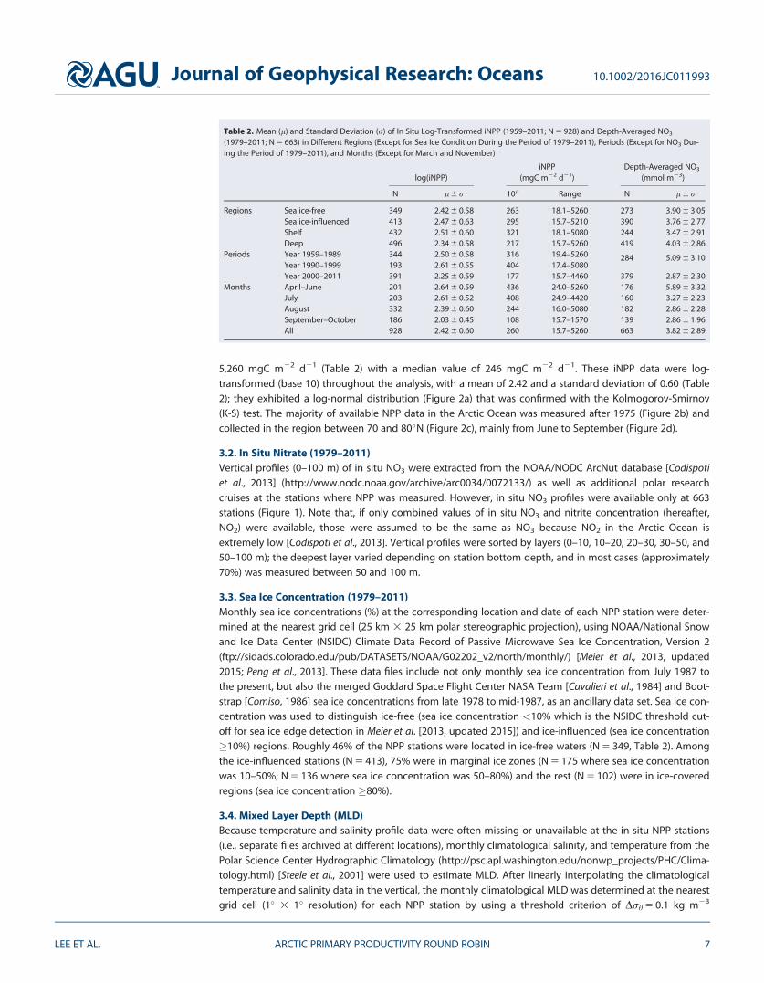

minus2 minus1 0 1 2 3
minus3
minus2
minus1
0
1
2
Normalized uRMSDN
orm
aliz
ed b
ias
(a)
Sea
minusic
e
iceminusfree (sea ice concentration10)iceminusinfluenced (sea ice concentrationgt10)
10 200
1
2
3
10
20
30
Nor
mal
ized
Sta
ndar
d D
evia
tion
10
20
30
uRMSD
minus040 000030
060
090
100
Correlation Coefficient
(b)
minus2 minus1 0 1 2 3
minus3
minus2
minus1
0
1
2
Normalized uRMSD
No
rmal
ized
bia
s
(c)
Dep
th
shallow (depth200m)deep (depthgt200m)
10 200
1
2
3
10
20
30
Nor
mal
ized
Sta
ndar
d D
evia
tion
10
20
30
uRMSD
minus040 000030
060
090
100
Correlation Coefficient
(d)
minus2 minus1 0 1 2 3
minus3
minus2
minus1
0
1
2
Normalized uRMSD
No
rmal
ized
bia
s
(e)
Dec
ade
1959~19891990minus19992000minus2011
10 200
1
2
3
10
20
30N
orm
aliz
ed S
tand
ard
Dev
iatio
n
10
20
30
uRMSD
minus040 000030
060
090
100
Correlation Coefficient
(f)
minus2 minus1 0 1 2 3
minus3
minus2
minus1
0
1
2
Normalized uRMSD
No
rmal
ized
bia
s
(g)
Sea
son
AprminusJunJulAugSepminusOct
10 200
1
2
3
10
20
30
Nor
mal
ized
Sta
ndar
d D
evia
tion
10
20
30
uRMSD
minus040 000030
060
090
100
Correlation Coefficient
(h)
Figure 4 (a c e and g) Target and (b d f and h) Taylor diagrams illustrating relative model performance in reproducing iNPP as a func-tion of (Figures 4a and 4b) sea ice condition ice-free region (sea ice concentration 15) versus ice-influenced region (sea ice concentra-tion gt15) (Figures 4c and 4d) depth shelf (200 m) versus deep (gt200 m) (e and f) simulation period (1959ndash1989 1990ndash1999 and2000ndash2011) and (g and h) month (AprilndashJune July August and SeptemberndashOctober)
Journal of Geophysical Research Oceans 1010022016JC011993
LEE ET AL ARCTIC PRIMARY PRODUCTIVITY ROUND ROBIN 12
coefficients assigned to distinct phytoplankton groups represented in the model [eg Aumont et al 2015]and thus result in differing Zeu for the same incoming PAR These differences may account for the early neg-ative bias in the participating model runs but do not (yet) point to either phytoplankton bloom physiologyor phenology processes being preferentially affected
44 Model Skill Assessment of Vertical Profiles of NPP and NO3
On a pan-Arctic scale the models had a strong tendency to underestimate the observed mean NPP at vari-ous depths eight out of 19 models had negative bias at all depth layers (Figure 5a) Note that not all themodels provided vertical profiles of NPP and NO3 (see Table 1) When the model standard deviation wassmaller than the observed one (2uRMSD) mean NPP was mostly underestimated (Figure 5a) But whenthe model standard deviation was larger than the observed one (1uRMSD) mean NPP was mostly under-estimated only between 0 and 20 m and overestimated between 30 and 100 m (Figure 5a) Deep NPP (50ndash100 m mean RMSD of 127) was better estimated than surface NPP (0ndash10 m mean RMSD of 148) in termsof RMSD since both bias and uRMSD became less at depth
Unlike NPP nine of 19 models overestimated mean NO3 at all depth layers while four models (Models 5 10 13and 20) underestimated mean NO3 except at the deepest layer (50ndash100 m) (Figure 5c) Model bias was lowestat depth such that mean NO3 concentration in the deep layer was better reproduced than in the surface layer(mean bias of 029 and 131 respectively) while the correlation coefficient was slightly higher at the surface (Fig-ure 5d) Furthermore the range of model bias for NO3 became wider (ie more scattered both in negative andpositive y axis) when the model standard deviations were smaller than the observed one (2uRMSD) However
minus2 minus1 0 1 2 3minus2
minus1
0
1
2
3
4
Normalized uRMSD
No
rmal
ized
bia
s
NP
P p
rofil
eN
PP
pro
file
NP
P p
rofil
eN
PP
pro
file
(a)
NP
P p
rofil
e
minus2 minus1 0 1 2 3minus2
minus1
0
1
2
3
4
NO
3 pro
file
NO
3 pro
file
NO
3 pro
file
NO
3 pro
file
Normalized uRMSD
No
rmal
ized
bia
s
(c)
NO
3 pro
file
0minus10m10minus20m20minus30m30minus50m50minus100m
10 200
1
2
3
10
20
30
Nor
mal
ized
Sta
ndar
d D
evia
tion
10
20
30
uRMSD
minus040000
030
060
090
100
Correlation Coefficient
(b)
10 200
1
2
3
10
20
30
Nor
mal
ized
Sta
ndar
d D
evia
tion
10
20
30
uRMSD
minus040000
030
060
090
100
Correlation Coefficient
(d)
Figure 5 (a and c) Target and (b and d) Taylor diagrams of vertical profiles in (Figures 5a and 5b) NPP (mgC m23 d21) and (Figures 5c and5d) (NO3) (mmol m23) which were grouped at given depth layers 0ndash10 m 10ndash20 m 20ndash30 m 30ndash50 m and 50ndash100 m
Journal of Geophysical Research Oceans 1010022016JC011993
LEE ET AL ARCTIC PRIMARY PRODUCTIVITY ROUND ROBIN 13
no significant difference in terms of uRMSD was exhibited between the depth layers (K-S test at a 5 level of sig-nificance) Overall performance of the models for NPP and NO3 was not significantly different within each depthlayer although correlation coefficients were higher for NO3 (Figures 5b and 5d) In general the models per-formed better in reproducing NO3 and NPP in the deepest layer (50ndash100 m) than at the surface (0ndash10 m)
45 Regional iNPP and NO3 ClimatologiesTo illustrate climatological spatial patterns and compare with regional iNPP estimated from each modelavailable in situ iNPP was projected onto the Equal-Area Scalable Earth Grid (EASE-Grid) map (100 km spatialresolution) by averaging data within each grid cell (Figure 6a) EASE-Gridded model iNPP was then averagedacross all models in each grid cell and compared to in situ climatological iNPP in six different regions of theArctic Ocean where NPP was frequently measured between 1959 and 2011 (Figures 6bndash6g) In situ andmodel iNPP exhibited no significant linear relationship on 10000 km2 basis (Figures 6c and 6f) and region-ally the lowest WS (Table 4) in the Chukchi and Greenland Seas both are influenced by inflow from subpo-lar latitudes In addition mean iNPP was most underestimated in the Canadian Archipelago and theGreenland Sea (Figures 6d and 6f) where ME was lowest (Table 4) Hence iNPP was least reproduced region-ally in the Greenland Sea in terms of intermodel mean (ie bias) as well as variability (ie WS and ME) As agroup the models performed best in the interior regions of the Arctic Ocean such as the Beaufort Sea andthe central Arctic Basin (Figures 6b and 6e) where NPP is relatively low (Figure 6a) and surface nutrients are
Figure 6 (a) In situ iNPP (mgC m22 d21) projected on the EASE-Grid map is shown (bndashg) Average model estimates with an error bar (61 standard deviation from the multimodel mean)in each grid cell were regionally compared to in situ values in Figure 6b the Beaufort Sea 6c the Chukchi Sea 6d Canadian Archipelago 6e the central Arctic Basin 6f the Greenland Seaand 6g the Barents Sea all inserts have the same axis units as in Figure 6f In each plot the solid-line shows a slope of 10 and the dashed line is a linear regression fit if significant(plt 005) The correlation coefficient (r) with degrees of freedom (df 5 number of grid cells22) are shown in the upper left A red circle with error bars indicates the regional average ofin situ (x axis) and modeled (y axis) iNPP
Journal of Geophysical Research Oceans 1010022016JC011993
LEE ET AL ARCTIC PRIMARY PRODUCTIVITY ROUND ROBIN 14
depleted toward the end of the growing season [Codispoti et al 2013] At the larger pan-Arctic scale modelskill for iNPP was higher than for most individual regions except where iNPP was best estimated ie theBeaufort Sea (WS and ME) and the Central Arctic Basin (WS Table 4)
Analogously in situ and modeled NO3 were also processed onto the EASE-Grid map in the deep layer (50ndash100 m Figure 7a) as well as at the surface (0ndash10 m Figure 8a) Again the models better reproduced theregional mean NO3 at the deepest layer overall (Figures 7bndash7g) However models notably underestimateddeep NO3 variability in the inflow Chukchi (Figure 7c) and Barents (Figure 7g) Seas (r5 2008 and r 5 023respectively) (see Table 4) On the contrary at the surface the models exhibited a tendency to overestimatemean NO3 (Figures 8bndash8g) This bias was smaller in the Greenland and Barents Seas (Figures 8f and 8grespectively) and highest in the interior regions of the Arctic Ocean (Figures 8b and 8e) where in situ surfaceNO3 is depleted at the end of summer and NPP is relatively low compared to that in other regions (Figures8a and 6a respectively) [Codispoti et al 2013] Model skill scores (Table 4) indicate that the regions wherethe models have the best skill in reproducing iNPP are also the ones where they exhibited the least skill inreproducing mean surface NO3 ie the Beaufort Sea and central Arctic Basin
46 Regional MLD Zeu and Sea Ice Concentration ClimatologiesUsing the same approach as in section 45 the regional mean MLD was relatively better estimated in theBarents and Greenland Seas (ie highest WS and ME in Table 4) and least reproduced in the Chukchi Seawhere MLD was consistently overestimated (Figure 9a) Moreover the highest regional model skills in sur-face NO3 were also calculated in the Barents and Greenland Seas But they do not necessarily appear toinfluence iNPP estimates ie poorly simulated iNPP especially in those regions Compared to the variablespreviously analyzed Zeu had the least amount of field data especially in the Barents and Greenland Seasand its mean was largely overestimated (Figure 9b) indeed incoming PAR onto the surface ocean will bevery different in open waters versus snow and ice-covered waters in the same latitude and season In theabsence of additional biological light-relevant parameters the assessment of model estimates of Zeu pro-vides a limited understanding of phytoplankton light utilization as it does not take into account that modelphytoplankton will differ in their response to the same light field Sea ice concentration is a logical next fac-tor to consider its model skill response is different from region to region and is mostly underestimated inthe Greenland Sea and overestimated in the Barents Sea (Figure 9c) In the Chukchi Sea mean sea ice con-centration was best estimated but iNPP was still rather poorly estimated when compared to other regions(Table 4) as indicated earlier While more high WS and ME model skill scores were shown for MLD and seaice concentration among the different regions no single environmental factor showed consistently highmodel skill for all regions indeed correlation analysis (not shown) between iNPP and any one environmen-tal factor ME skill suggests a possible robust relationship with Zeu instead despite individual lower skillscores Hence iNPP model skill was constrained by different factors in different Arctic Ocean regions Pan-Arctic averaging did not necessarily improve model skill for iNPP and associated variables over regional(Table 4) and subregional (Figure 6) scales
Table 4 Willmott Skill (WS) Score Ranging Between 0 and 1 for a Perfect Model and Modeling Efficiency (ME) Between -1 and 1 for aPerfect Model of Multimodel Mean iNPP Surface and Deep NO3 Zeu Sea Ice Concentration and MLD in Six Regions of the Arctic Ocean
Regions Model Skill
Variables
iNPP Surface NO3 Deep NO3 Zeu Sea ice MLD
Chukchi WS 049 046 033 067 090 008ME 2006 2365 2027 2055 072 2264
Canadian Archipelago WS 061 049 059 031 054 046ME 2032 2231 030 2128 2004 2449
Beaufort WS 077 009 051 065 085 025ME 036 2135 015 001 064 2764
CentralArctic Basin
WS 075 013 046 045 067 034ME 009 2383 015 001 039 2225
Barents WS 063 080 025 063 072 093ME 2010 042 2014 2038 015 079
Greenland WS 033 074 074 027 040 090ME 2284 009 041 2247 2019 062
Pan2Arctic WS 067 063 047 067 080 092ME 012 2084 007 2025 050 074
Journal of Geophysical Research Oceans 1010022016JC011993
LEE ET AL ARCTIC PRIMARY PRODUCTIVITY ROUND ROBIN 15
5 Discussion
It has long been known that marine primary production is controlled by the interplay of the bottom-up fac-tors of light and nutrients whose availability is a function of physical andor biological processes Earlierintercomparison studies for the Arctic Ocean emphasized the importance of a realistic representation ofocean physics [Popova et al 2012] in particular vertical mixing and nutrient concentration for accurate Arc-tic Ocean ecosystem modeling Five BOGCMs manifested similar levels of light limitation owing to a generalagreement on the simulated sea ice distribution [Popova et al 2012] On the other hand the ESMs partici-pating in the Vancoppenolle et al [2013] study showed that Arctic phytoplankton growth was more limitedby light related to sea ice than by nutrient availability for the period of 1980ndash1999 Furthermore with thelarge uncertainties on present-day nitrate in the sea ice zone ESMs used in the framework of the CMIP5exercise were inconsistent in their future projections of primary production and oligotrophic condition inthe Arctic Ocean [Vancoppenolle et al 2013] The need to quantify the relative role of environmental andecological controls on NPP in the heterogeneous seasonally ice-covered Arctic Ocean remains
In our study iNPP model skill was linked to different environmental variables in the various Arctic Oceanregions The models exhibited relatively lower skill in reproducing iNPP in high to very high production Arc-tic Ocean regions [in the sense of Codispoti et al 2013] (ie the Chukchi and Greenland Seas in Table 4 andFigure 6) despite higher model skill in physical parameters such as sea ice concentration or MLD respec-tively Model performance in estimating iNPP was also more related to the model skill of sea ice conditions(and Zeu) than NO3 (and MLD) in the extremely low production regions [in the sense of Codispoti et al2013] (ie the Beaufort Sea and central Arctic Basin in Table 4 and Figure 8) where in situ NO3 is virtually
Figure 7 Same as Fig 6 but for NO3 (mmol m23) in the deep layer (50ndash100 m)
Journal of Geophysical Research Oceans 1010022016JC011993
LEE ET AL ARCTIC PRIMARY PRODUCTIVITY ROUND ROBIN 16
depleted (ie almost no variability in the in situ data) Field studies in the Arctic Ocean have failed to dem-onstrate any statistical relationship between phytoplankton biomass or productivity and ambient nutrientconcentrations or nutrient utilization rates in eastern Arctic waters [Harrison and Platt 1986 Harrison andCota 1991] while phytoplankton biomass and productivity were significantly related to incident radiation[Harrison and Cota 1991 but see Tremblay et al 2015] Hence simulated iNPP was close to in situ values insuch low production regions because light fields were likely better reproduced even though surface NO3
was systematically biased (Figures 8b and 8e)
Our study also showed that simulations of surface NO3 (nutrient) and Zeu (light) associated with MLD (con-trolling the depth horizon where phytoplankton cells are) exhibited low model skill in most of the regions(Table 4) being lowest in the interior of the Arctic Ocean This observation is not necessarily new [Popovaet al 2012 Vancoppenolle et al 2013] but one should be cautious when interpreting this result becausethese three simulated parameters were positively biased (ie means usually overestimated) (Figures 8 and9) For example the simulated mean surface NO3 was vastly overestimated especially in the low-productivity nutrient-depleted interior regions of the Arctic Ocean ie the Beaufort Sea and the centralArctic Basin where model and in situ iNPP agreed best (Figures 6b and 6e Table 4) At least on a regionalscale the overestimation of surface NO3 possibly stems from spurious vertical mixing between the uppermixed layer and deeper water in the model simulations resulting in excessive nutrient supply into the sur-face layer For example except in the Greenland and Barents Seas MLD mean and variability were poorlyestimated (Table 4) and mostly overestimated (Figure 9a) by as much as twofold possibly resulting inhigher nutrients at the surface Alternatively a physiological perspective may be examined based on the
Figure 8 Same as Fig 6 but for NO3 (mmol m23) in the surface layer (0ndash10 m)
Journal of Geophysical Research Oceans 1010022016JC011993
LEE ET AL ARCTIC PRIMARY PRODUCTIVITY ROUND ROBIN 17
most common model parameterization ofphytoplankton growth (ie a combinationof a nutrient term a light term atemperature-dependent growth term anda maximum growth rate over a daily peri-od) Then the overestimated NO3 may becaused by insufficient phytoplankton nutri-ent uptake (ie too low a rate for Arcticwaters) since NPP was overall underesti-mated by most of the models Phytoplank-ton nitrate uptake is strongly dependenton both temperature (ie less at coldertemperatures) [Lomas and Glibert 1999]and irradiance (ie photoinhibited athigher levels) [Hu and Smith 1998] andbecomes more dependent on their com-bined effect in the simultaneously coldand dark Arctic waters during the transi-tion to spring conditions [Tremblay et al2006] It is likely that several of the modelshave globally relevant phytoplanktonphysiological parameter values that aretoo high and may thus not correspond tothe lower and narrower ranges requiredby Arctic (or polar) phytoplankton SomeArctic phytoplankton species are shade-acclimated especially in spring thoughmost available data are for summer light-adjusted phytoplankton [Sakshaug 2004Harrison et al 1982] Arctic phytoplanktoncommunity structure appears to changetoward smaller cells in response to warm-ing both in the field and in experiments [Liet al 2009 Tremblay et al 2009 Coello-Camba et al 2014 2015] that may havedifferent nutrient uptake kinetics [Lovejoyet al 2007] while individual phytoplank-ton species may have narrower tempera-ture ranges for optimal growth usually incombination with light requirements [Har-rison and Platt 1986 Vernet et al 2012]These phenological changes will requirethe inclusion of multiple phytoplanktonsize classes in models andor differentphysiological rates
The distribution of NO3mdashhence its poten-tial availability for NPPmdashdiffered by depth(Figure 5c) as well as region (Table 4) Aless ecological and more pragmatic expla-nation for the overestimation of surfaceNO3 may be that the models are incapableof reproducing the vertical mixing dynam-ics required (as shown by the ubiquitousMLD overestimation Figure 9a) no evident
Figure 9 Modeled MLD Zeu and sea ice concentration bias (a) MLD biasbetween 15 model mean and monthly climatological MLD (m) (b) Zeu biasbetween 9 model mean and in situ Zeu (m) and (c) sea ice concentration biasbetween 19 model mean and satellite-derived values ()
Journal of Geophysical Research Oceans 1010022016JC011993
LEE ET AL ARCTIC PRIMARY PRODUCTIVITY ROUND ROBIN 18
relationship was found between vertical resolution and skill in surface NO3 among the participating models(not shown) Indeed the future Arctic Ocean may produce less NPP per unit area due to less surface NO3 [egVancoppenolle et al 2013] resulting from enhanced freshening [Coupel et al 2015] as also hypothesized byMcLaughlin and Carmack [2010] Unlike surface NO3 deep NO3 was more realistically reproduced pan-Arcticwide in terms of the multimodel ensemble mean values at 100 km grid scales (average symbols in Figure 7)Indeed deep NO3 and sea ice concentration (ie measured as ME) were relatively well explained by the multi-model ensemble in at least four regions (Table 4) Still deep NO3 (50ndash100 m) was relatively poorly estimatedin the inflow Barents and Chukchi Seas in terms of correlation coefficients (Figures 7c and 7g) and regionalmeans (WS in Table 4) Those two regions are strongly influenced by horizontal advection of sub-Arctic inflowwaters which contribute to the nutrient supply into the Arctic Ocean via the Bering Strait and Fram StraitBarents Sea openings [eg Carmack and Wassmann 2006 Wassmann et al 2015] Torres-Valde et al [2013]estimated the volume and NO3 transports into the Arctic Ocean based on a combination of modeled and insitu velocity fields and nutrient sections total volume and NO3 transport into the Arctic Ocean at depth corre-sponded to 20 and 80 through the Bering Strait and the Barents Sea opening respectively (ie a signifi-cant contribution) Smith et al [2011] also showed the greater relative importance of this advective nutrientinput compared to vertical mixing in the Arctic Ocean
Involvement of a light-driven component of the simulation of NPP is provided by the fact that Zeu was gen-erally overestimated in all Arctic regions by most of the nine models that provided this field (Figure 9b) Thesimulated Zeu (9 model mean of 56 m) compared to the mean in situ Zeu (37 m) was deeper than MLD (18model mean of 23 m and climatological mean of 16 m) Possible explanations for the Zeu overestimationmay include the prescription of lower turbidity levels than the typical values in the Arctic Ocean In addition(or instead) the parametrization of light extinction in the water column may be associated with sea ice con-ditions ie the Zeu overestimation coupled with underestimation of sea ice concentration may result inlight being able to penetrate deeper into the water column during a simulation From a biophysical per-spective the self-shading effect caused by the presence of phytoplankton is considered in many of the par-ticipating models already Although we focused on model skill in estimating NPP not phytoplanktonbiomass the self-shading effect has been reported as negligible for high latitudes in sensitivity analyses[Manizza et al 2005] Yet other biogeochemical species like colored dissolved organic matter that couldreduce the light penetration into the water column are not represented in the models used in this study[Granskog et al 2012 Dutkiewicz et al 2015 Kim et al 2015] Nonetheless NPP was still underestimateddespite apparent light availability emphasizing a physiological coupling between light availability and lightrequirements by phytoplankton alternatively it suggests that low NPP would generate low phytoplanktonbiomass which would result in a deeper Zeu simply due to lack of light absorption
Given that the models overestimated surface NO3 and Zeu the simulated phytoplankton populations wouldexperience more nutrient and light availability which should have led to higher iNPP However the simulat-ed NPP was mostly underestimated in all regions of the Arctic Ocean clearly indicating that surfacenutrients were not the primary limiting factor for the underestimated iNPP in these model simulationsBecause the regions with higher model skill at estimating iNPP coincided with better model skill in Zeu andsea ice concentration especially in low production regions the amount of shortwave radiation or PAR trans-mitted through sea ice could account partly for underestimating iNPP [Babin et al 2015] Our findings fur-ther suggest that biological processes (ie phytoplankton growth and photosynthesis) were possiblymisrepresented by the model configurations run for this Arctic Ocean exercise A previous model intercom-parison study for lower latitudes pointed out that an improved understanding of the temperature effect onphotosynthesis and a better parameterization of the maximum photosynthetic rate are required [Carr et al2006] Hence one might argue that phytoplankton growth functions were not adequately parameterizedespecially for colder high latitudes in many models resulting in lesser utilization of surface nutrients This isdebatable in the Beaufort Sea where the effect of temperature on photosynthetic parameters over the insitu range observed (22 to 88C) was found not significant [Huot et al 2013] Furthermore a large variabilityin photosynthetic parameters and half-saturation constants exists in Arctic ecosystem models as recentlyreviewed by Babin et al [2015] during a model sensitivity exercise they showed that temperature was notas strong a limiting factor for phytoplankton growth as others (ie light and nitrate) Although it could bethat nutrients light and temperature relationships need to be adjusted to improve model skill in the ArcticOcean such a regional tuning is however not possible for global BOGCMs and ESMs
Journal of Geophysical Research Oceans 1010022016JC011993
LEE ET AL ARCTIC PRIMARY PRODUCTIVITY ROUND ROBIN 19
Simulated NPP may be low due to not only limiting factors but also because of too little biomass egthrough excessive loss of carbon from or in the upper water column Vertical export of organic matter isparameterized in all models The organic carbon to organic nitrogen stoichiometric ratio in sinking particu-late matter has been shown not to be constant in Arctic waters [Tamelander et al 2013 Michel et al 2006]as assumed in most models Arctic phytoplankton are also known to have large exudation levels during cer-tain phases of their growth cycle [Vernet et al 1998 Laroche et al 1999] which promotes the formation ofsinking aggregates resulting in significant carbon export from the surface layer when large phytoplanktoncells dominate [Reigstad et al 2011 Wassmann et al 2006] Changes in phytoplankton species compositionand bloom phenology in Arctic waters are also being reported These changes include shifts toward smallercells possibly with different physiology especially in the freshening Beaufort Sea and Canadian Arctic Archi-pelago [Li et al 2009 Tremblay et al 2009] which will again affect vertical export fluxes Changes in bloomphenology have been described as lengthening bloom periods or even the presence of fall blooms(reviewed by Babin et al [2015] Michel et al [2006 2015]) However these changes are fairly recent and like-ly not yet simulated by models nor captured by the in situ data used for our exercise despite covering fivedecades back (ie diminishing the likelihood of an effect in our field data set)
If bottom-up factors were not the main or sole controls on phytoplankton productivity grazing could benot only may grazers reduce NPP but they also regulate vertical flux If simulated grazing rates were toohigh then the resulting nutrient concentrations would be much higher than the values of the high satura-tion constants used This scenario was ruled out for high latitudes by a PISCES-based model simulation inwhich bottom-up controls did dominate [Aumont et al 2015] On the other hand the northward advectiveinflow of sub-Arctic water has been reported to also carry significant zooplankton biomass [Wassmannet al 2015] Hence it is possible that the Arctic Ocean primary production in model simulations might bereduced under increased grazing pressure from such sub-Arctic (expatriate) zooplankton Such a hypotheti-cal extension of sub-Arctic grazing influence to the interior regions of the Arctic Ocean is not currently sup-ported by observations [Kosobokova and Hopcroft 2010] Much is changing with respect to trophicstructure in the Arctic Ocean including grazer community composition and biodiversity [Bluhm et al 2015]all of which may or may not be simulated by the models with consequences for estimating iNPP Howeverwe currently lack a comprehensive review and climatology for in situ micro meso and macrozooplanktongrowth and grazing rates in the Arctic Ocean to broadly assess model relative skill
Our use of an in situ NPP database allowed the assessment of model skill in ice-influenced as well as in ice-free waters overcoming a limitation encountered by previous model intercomparison exercises for the Arc-tic Ocean [eg Popova et al 2012 Vancopenolle et al 2013] that depended on satellite-derived NPP whichis not available for ice-covered regions Regardless of whether sea ice was present or not the mean and var-iance of in situ iNPP were almost identical confirming that the ice-influenced regions could be as produc-tive as the ice-free regions (Table 2) It should be noted that the similarity could be due to biased seasonalcoverage by field studies in ice-free waters introducing more measurements collected in late summer andfall (ie September) thus lowering the ice-free iNPP average (not shown) Alternatively the similarity in sim-ulated iNPP values in ice-free and ice-influenced areas could result from the averaging of regional differ-ences previously observed in field and satellite-derived NPP data [eg Arrigo et al 2012 Hill et al 2013Ardyna et al 2013] as well as in model simulations [eg Zhang et al 2015] Recently Jin et al [2016]showed that simulated under-ice production is also regionally different (ie higher in the Arctic shelvespossibly due to enhanced nutrient supply) [Zhang et al 2015] but not necessarily related to the recentdecrease in sea ice concentration especially in marginal ice zones Regardless of whether NPP was mea-sured in deep versus shallow areas or ice-influenced versus open water regions model skill for iNPP differedlittle on such spatial scales
Time did make a difference however Model skill varied from decade to decade and higher model skill wasfound for the most recent decade (Figures 4e and 4f) when in situ iNPP and NO3 were lower (Table 2) sincethe models performed better with low iNPP For example on a pan-Arctic scale in situ carbon uptake ratesdecreased to 177 mg C m22 d21 (N 5 344 2000ndash2011) compared to 316 mg C m22 d21 in the earlier deca-des (N 5 391 1959ndash1989) Similarly in situ depth-averaged NO3 decreased from 51 mmol m23 (N 5 2841979ndash1999) to 29 mmol m23 (N 5 379 2000ndash2011) These decreases likely resulted from differences in geo-graphical sampling distribution between decades (Figure 1) For example during 2000ndash2011 more datawere available from the large Canadian and International Polar Year programs in low production regions
Journal of Geophysical Research Oceans 1010022016JC011993
LEE ET AL ARCTIC PRIMARY PRODUCTIVITY ROUND ROBIN 20
such as the Beaufort Sea and the central Arctic Basin (Figure 1c) Not all of the participating models cap-tured these decreasing changes in simulated iNPP and NO3 (not shown) However regardless of whethermodel iNPP estimates increased or decreased over the most recent decade simulated iNPP values becamemore comparable to in situ values on a pan-Arctic scale such that model skill was seen to be improved inmore recent years (Figures 4e and 4f) On a seasonal time-scale the models generally performed poorly inthe beginning of the growing season (AprilndashJune) compared to later months (Figures 4g and 4h) For somemodels this could be due to insufficient penetration of winter mixing as the main mechanism controllingbasin-scale patterns of nutrient supply [eg Popova et al 2012] though as stated earlier MLD was overesti-mated overall (Figure 9a) Also occurring at this time is the critical balance between the onset and phenolo-gy of sea ice melting ice algal bloom andor phytoplankton bloom small mismatches in timing amongthem resulted in a large variability of simulated phytoplankton availability especially at the Arctic marginalseas [Ji et al 2013]
Model quantification of biogeochemical processes is highly dependent on how accurately physical fieldsare simulated [Friedrichs et al 2006 Popova et al 2012] Submesoscale physical features are especiallyimportant to biogeochemical processes affecting the horizontal and vertical distribution of nutrients andphytoplankton biomass [Watanabe et al 2014] Most of the participating models are developed on globalscales and only four of them are regional models of the order of 10 km resolution (Table 1) The Rossby radi-us of deformation is dramatically reduced with increasing latitude and it becomes less than 10 km in theArctic Ocean Hence those models with resolution of the order of 10ndash100 km may not adequately resolvesubmesoscale physical features at the surface layer that are likely critical for Arctic biogeochemical process-esmdashin particularmdashregionally [Timmermans et al 2012] rather than larger-scale physical processes deter-mining the response of the pan-Arctic marine ecosystem High spatial resolution models or more Arctic-appropriate parameterizations and closures are necessary to capture small-scale physical processes such aseddies tides fronts internal waves as well as interactions between shelf and open ocean or sea and ice pro-cesses that can influence phytoplankton growth especially in high-productivity coastal shelf regions adja-cent to sub-Arctic waters Indeed regionally model skill patterns are contradictory such that the GreenlandSea has a very closely simulated surface and deep NO3 and MLD (Table 4) but the least skill in simulated seaice concentration (Figure 9c) yet it has the lowest skill in iNPP underestimating it (Figure 6f) Converselythe Beaufort Sea shows medium skill in deep NO3 least skill in surface NO3 (overestimating concentrations)and yet the best skill in iNPP (Table 4)mdashstill underestimating iNPP and its variability (Figure 6b) though lessthan other Arctic Ocean subregions Assuming improved parameterization of nutrient light and tempera-ture relationships of phytoplankton growth a higher spatial resolution model could potentially produce sig-nificant subregional features [eg Yool et al 2015] as mesoscale and submesoscale processes have beenshown to stimulate biological productivity in lower latitudes [McGillicuddy et al 1998 Oschlies and Garcon1998 Levy et al 2001] Finally coastal regions characterized by elevated primary productivity are also notproperly resolved by a coarse model grid in general [Aumont et al 2015] Higher resolution in ecosystemcomplexity has already been shown to lead to improved realism of BOGCM high latitude simulations withthe addition of slow growing macrozooplankton leading to the successful representation of the differentbloom dynamics in the Southern Ocean [Le Quere et al 2016] Much effort is now being applied in themodeling community to introduce high-resolution strategies into BOGCMs especially those regionallyfocused on the Arctic Ocean [Interagency Arctic Research Policy Committee 2013] with the hope that repro-ducing meso and submesoscale processes and features will improve their predictive skill for iNPP and otherbiogeochemical properties in the Arctic Ocean
6 Summary and Recommendation
Using in situ satellite-derived and climatological data we have analyzed model estimates of iNPP and NO3
associated with physical variables such as MLD Zeu and sea ice concentration from 21 BOGCMs and ESMsduring the period of 1959ndash2011 although the time span of simulation as well as the initialization and forc-ing were different among the participating models No models fully reproduced the variability of in situmeasurements whereas some of them exhibited almost no bias Generally the models captured the spatialfeatures of the iNPP distribution lower iNPP in the interior regions and higher iNPP in the inflow regionsThe models exhibited different regional characteristics in estimating iNPP since each modelrsquos skill was afunction of environmental factors with distinctive sensitivity in one region versus another For example
Journal of Geophysical Research Oceans 1010022016JC011993
LEE ET AL ARCTIC PRIMARY PRODUCTIVITY ROUND ROBIN 21
MLD and NO3 were reproduced well in the Atlantic-side inflow and outflow regions Zeu had greater skill inthe interior regions and sea ice concentration was reasonably well estimated everywhere except in theGreenland Sea Most of the models generally underestimated mean iNPP in spite of overestimating Zeu andsurface NO3 especially in the Chukchi and Greenland Seas where mean in situ iNPP is high Regionallymodel iNPP was best estimated in the regions where simulated surface NO3 was most overestimated rela-tive to in situ values and where both sea ice concentration and Zeu were reproduced well such as the Beau-fort Sea and the central Arctic Basin By contrast iNPP exhibited the largest model-data disagreement in theGreenland Sea where the simulated surface NO3 and MLD had greater model skill but sea ice concentrationhad lower model skill
The Arctic Ocean appears to be experiencing a fundamental shift from a polar to a temperate mode whichis likely to alter its marine ecosystem [Yool et al 2015 Wassmann et al 2015] Under a changing climatesea ice loss shifts in composition and distribution of phytoplankton functional types and bloom phenologychanges already play a role in the Arctic Ocean marine ecosystem [eg Li et al 2009 Ardyna et al 2014]Globally changes in nutrient and light availability have emerged as the most important determinants inmodels for alterations in simulated growth rates with light generally playing a lesser role except for thevery high latitudes particularly the Arctic Ocean [Laufkeurootter et al 2015] At these high latitudes tempera-ture does not appear to play a physiological role but could well play an ecological role of controlling phyto-plankton bloom composition and phenology [Babin et al 2015] Thus ecosystem processes and algalphysiology in models need to be carefully parameterized for the Arctic Ocean in order to better quantifyuncertainties in estimating primary production including under-ice primary production and ice algae pro-duction [Leu et al 2015 Jin et al 2016] enhanced functional types for all levels of the marine food web[Babin et al 2015] and the role of horizontal advection of planktonic organisms versus their vertical export[Wassmann et al 2015] Furthermore it is necessary to resolve submesoscale physical processes to decidethe apparently contradictory bottom-up controls of NPP and the resulting biogeochemical cycles in the var-ious subregions of the Arctic Ocean with the hope that BOGCMs and ESMs perform within the uncertaintydue to natural variability Last but not least models will continue to improve their skill when additional vali-dating data sets and climatologies are gathered and openly shared for relevant biogeochemical physiologi-cal and ecological variables in the Arctic Ocean
Appendix A Brief Description of Participating Models
A1 Model 1HYCOM-NORWECOM [Samuelsen et al 2015] is a regional coupled physical-biogeochemical model with 11compartments in the biogeochemical model The physical model is the Hybrid Coordinate Ocean Model(HYCOM) [Bleck 2002] adapted to the North Atlantic and Arctic Ocean [Bertino and Lisaeter 2008] The mod-el encompasses the entire North Atlantic and has open lateral boundaries at the Bering Strait in the PacificOcean and near the equator between 38S and 168S in the Atlantic Ocean the model is relaxed toward clima-tological values at the lateral boundaries The model is forced by ERA-Interim [Dee et al 2011] hydrologicalforcing from TRIP [Oki and Sud 1998] but does not include tidal forcing The sea ice model uses an elastic-viscous-plastic (EVP) rheology [Hunke and Dukowicz 1997] while thermodynamics are described in Drangeand Simonsen [1996] NORWEgian ECOlogical Model (NORWECOM) [Aksnes et al 1995 Skogen and Soslashiland1998] is coupled online to HYCOM and uses HYCOM facility for advection of tracers and has the same time-step as the physical model The current model version includes two classes of phytoplankton (diatom andflagellates) two classes of zooplankton (meso and microzooplankton) derived with the same formulationfrom the model ECOHAM4 [Peuroatsch et al 2009] three types of nutrients (N P and Si) and detritus (N and P)biogenic Si and oxygen (O2) Additionally riverine nutrient loads are based on the results from the Global-NEWS model [Seitzinger et al 2005] The model assumes a constant element ratio (ie Redfield) as well asconstant chlorophyllN ratio in phytoplankton In the model light does not propagate through sea icetherefore the model is not expected to yield realistic primary production and nutrients in areas with thinice cover where light actually is available for primary production
A2 Model 2This global biogeochemical model (1998ndash2014) uses the PISCES formulation on the horizontal curvilineargrid ORCA025 and 75 vertical levels It is forced offline by daily fields of an ocean circulation simulation
Journal of Geophysical Research Oceans 1010022016JC011993
LEE ET AL ARCTIC PRIMARY PRODUCTIVITY ROUND ROBIN 22
Nucleus for European Modelling of the Ocean (NEMO)-Ocean PArallelise (OPA) (version 31) [Madec 2008]Atmospheric forcings are 3 hourly ERA-Interim reanalysis product with the CORE bulk formulation There isno assimilation of physical data The sea ice model is the Louvain la Neuve sea Ice Model version 2 (LIM2)with EVP rheology [Fichefet and Morales Maqueda 1997] PISCES (volume 2) [Aumont et al 2015] is a modelof intermediate complexity designed for global ocean applications and is a component of the NEMO model-ing system It has 24 prognostic variables and simulates biogeochemical cycles of O2 C and the mainnutrients controlling phytoplankton growth (NO3 ammonium (NH4) phosphate (PO4) silicate (SiO4) andFe) The model distinguishes four plankton functional types based on size two phytoplankton groups(nanophytoplankton and diatoms) and two zooplankton groups (micro and mesozooplankton) PISCEStraces three nonliving pools for small and big particulate organic carbon (POC) and semilabile dissolvedorganic carbon (DOC) Version 35 of NEMO-PISCES with default parameter set is used here The configura-tion is described and assessed in the Product User Manual and Quality Information Document (httpmarinecopernicuseudocumentsPUMCMEMS-GLO-PUM-001-018pdf and httpmarinecopernicuseudocumentsQUIDCMEMS-GLO-QUID-001-018pdf) Daily and monthly mean outputs are available on Coper-nicus Marine Service website (httpmarinecopernicuseu)
A3 Model 3This model is the Plankton Types Ocean Model 53 (PlankTOM53) biogeochemical model coupled to theNEMO (version 23) global ocean circulation model and sea ice model (LIM2) The biological model is a 26component marine pelagic ecosystem model including three phytoplankton components (diatoms cocco-lithophores and mixed phytoplankton) two zooplankton components (micro and mesozooplankton) DOCsmall and large detrital POC and particulate organic Fe detrital particulate Si and calcite and dissolved NO3SiO4 and Fe [Buitenhuis et al 2013] Each phytoplankton functional type has C chlorophyll and Fe compo-nents linked with a dynamic photosynthesis model [Buitenhuis and Geider 2010] The standard simulationwas spun up from 1920 to 1955 and for the purpose of this paper the optimized simulation was run from1956 to 2013 [Buitenhuis et al 2013]
A4 Model 4This model is the Plankton Types Ocean Model 10 (PlankTOM10) biogeochemical model coupled to theNEMO (version 31)-LIM2 ocean circulation and sea ice model The biological model is a 37 componentmarine pelagic ecosystem model including six phytoplankton components (diatoms coccolithophorespicophytoplankton N2-fixers phaeocystis and mixed phytoplankton) three zooplankton components(micro meso and macrozooplankton) bacteria DOC small and large detrital POC and particulate organicFe detrital particulate Si and calcite and dissolved NO3 SiO4 and Fe [Le Quere et al 2016] PlankTOM10 hasthe same dynamic photosynthesis model as PlankTOM53 (Model 3) In addition it has an improved repre-sentation of the difference between the high latitude Northern and Southern Hemisphere phytoplanktonblooms through the representation of slow growing macrozooplankton The different physical settingsresult in different overwintering macrozooplankton populations in turn leading to different trophic cas-cades and more realistic phytoplankton blooms [Le Quere et al 2016]
A5 Model 5The Carbon Ocean Biogeochemistry and Lower Trophics (COBALT) version 10 marine ecosystem modeluses 33 state variables to resolve global-scale cycles of C N P Si Fe calcium carbonate (CaCO3) O2 andlithogenic material [Stock et al 2014a] COBALT derives many elements of its biogeochemical formulationfrom the TOPAZ model (see Model 6) However COBALT enhances the resolution of planktonic food webdynamics to better understand the climate impacts on the flow of energy from phytoplankton to fish [Stocket al 2014b] The model includes three phytoplankton groups (small large and diazotrophs) and uses thevariable chlorophyllC formulation of Geider et al [1997] to estimate NPP Results contributed to this studywere conducted with the Modular Ocean Model (MOM) version 4p1 [Griffies 2012] with sea ice dynamics asdescribed in Winton [2000] The model was run on a global domain with a nominal spatial resolution of 18
and a tripolar Arctic grid The model uses 50 vertical layers with a nominal resolution of 10 m over the top200 m Simulations are forced with the Coordinated Ocean-ice Reference Experiment version 2 (CORE2)data set [Large and Yeager 2009] The 60 year forcing period was looped twice and results from the secondloop provided for this study Surface salinity is relaxed to observations with 2 month relaxation time-scale inorder to avoid salinity drifts characteristic of long integrations of ocean-ice simulations without fully
Journal of Geophysical Research Oceans 1010022016JC011993
LEE ET AL ARCTIC PRIMARY PRODUCTIVITY ROUND ROBIN 23
coupled atmosphere dynamics [Griffies et al 2009] Complete details of the simulation and model validationcan be found in Stock et al [2014a]
A6 Model 6Tracers of Ocean Phytoplankton with Allometric Zooplankton version 20 (TOPAZ2) is an ocean biogeo-chemical and ecological model developed at NOAArsquos Geophysical Fluid Dynamics Laboratory for globalEarth System Model simulations contributed to the 5th assessment report of the Intergovernmental Panelon Climate Change [Dunne et al 2012b2013] TOPAZ2 includes 30 tracers to describe the cycles of C NP Si Fe O2 alkalinity and lithogenic material as well as surface sediment calcite dynamics [Dunne et al2012a] TOPAZ2 considers three explicit phytoplankton groups (small large and diazotrophs) that utilizea modified growth physiology after Geider et al [1997] with Eppley [1972] temperature functionality andiron colimitation with luxury uptake after Sunda and Huntsman [1997] CO2NO3O2 stoichiometry is10616150 after Anderson [1995] NP is based on optimal allocation after Klausmeier et al [2004] Com-plete technical details are available in the supplementary information of Dunne et al [2013] Results con-tributed to this study were conducted with the MOM (version 4p1) [Griffies 2012] with sea ice dynamicsas described in Winton [2000] The model was run on a global domain with a nominal spatial resolution of18 and a tripolar Arctic grid The model uses 50 vertical layers with a nominal resolution of 10 m over thetop 200 m Simulations are forced with the CORE2 data set [Large and Yeager 2009] The 60 year forcingperiod was looped twice and results from the second loop provided for this study Surface salinity isrelaxed to observations with 2 month relaxation time-scale in order to avoid salinity drifts characteristicof long integrations of ocean-ice simulations without fully coupled atmosphere dynamics [Griffies et al2009]
A7 Model 7SINMOD is a model system that has been continuously developed over 30 years and includes a hydrody-namic and a sea ice module [Slagstad and McClimans 2005] an ecosystem module [Wassmann et al 2006]and stage resolved zooplankton models [Slagstad and Tande 2007] The hydrodynamic model is based onthe primitive Navier-Stokes equations and is established on a Z-grid [Slagstad and McClimans 2005] The icemodel is similar to that of Hibler [1979] and has two state variables ice thickness and ice concentration Theice momentum equation is solved together with an equation for the ice internal stress using the EVPdynamical model of Hunke and Dukowicz [1997] The ecosystem model includes nutrients (NO3 NH4 andSiO4) phytoplankton (diatoms and flagellates) bacteria heterotrophic nanoflagellates microzooplanktonand two mesozooplankters the Atlantic Calanus finmarchicus and the arctic C glacialis two compartmentsfor fast and slow sinking detritus DOC and sediments The model uses constant stoichiometry with a CNratio equal 76 based upon average data from the Barents Sea [Reigstad et al 2002] In the present studySINMOD data are from a pan-Arctic configuration with 20 km horizontal grid resolution and with 25 verticallayers Forcing fields includes atmospheric forcing from the ERA-Interim reanalysis (httpwwwecmwfint)[Dee et al 2011] tides from TPXO 62 model prescribed at open boundaries and freshwater run-off fromR-ArcticNet (httpwwwr-arcticnetsrunhedu) More details of the recent updates of SINMOD and themodel setup may be found in Slagstad et al [2015]
A8 Model 8The NorESM-OC is the ocean component of the Norwegian Earth System Model (NorESM) It is a coupledBOGCM which comprises the Miami Isopycnic Coordinate Ocean Model (MICOM) coupled with the Ham-burg Oceanic Carbon Cycle (HAMOCC)25 model [Schwinger et al 2016] HAMOCC consist of a Nutrient-Phytoplankton-Detritus-Zooplankton (NPDZ)-type ecosystem model where the primary production isformulated as a function of phytoplankton growth and nutrient concentration within the euphotic layer(fixed at 100 m) In addition to multinutrients (ie NO3 PO4 and dissolved Fe) colimitation the phyto-plankton growth is regulated by light availability and temperature The model adopts a generic singleclass phytoplankton and zooplankton compartment The particulate materials (ie POC biogenic opaland CaCO3) produced at the surface sink with constant velocities and are remineralized at depth The pro-duction of surface opal and CaCO3 is determined by the SiO4 availability at the surface Nonremineralizedparticles reaching the seafloor undergo chemical reactions with sediment pore waters bioturbation andvertical advection within the sediment module For the simulation produced in this study the NorESM-OCwas forced by the CORE2 atmospheric reanalysis data
Journal of Geophysical Research Oceans 1010022016JC011993
LEE ET AL ARCTIC PRIMARY PRODUCTIVITY ROUND ROBIN 24
A9 Model 9This model is the BiologyIceOcean Modeling and Assimilation System (BIOMAS) a coupled biophysicalmodel [Zhang et al 2010a] with four model elements an ocean circulation model a sea ice model a pelag-ic biological model and a sea ice algae model The ocean circulation model is based on the Parallel OceanProgram (POP) developed at Los Alamos National Laboratory [Smith et al 1992] and modified by Zhangand Steele [2007] so that open boundary conditions can be specified The POP ocean model is further modi-fied by Zhang et al [2010b] to incorporate tidal forcing from eight primary constituents [Gill 1982] The seaice model is a thickness and enthalpy distribution (TED) sea ice model [Zhang and Rothrock 2003 Hibler1980] with eight categories each for ice thickness ice enthalpy and snow depth It is adopted from thePan-arctic IceOcean Modeling and Assimilation System (PIOMAS) [Zhang and Rothrock 2003] and capableof assimilating satellite observations of sea ice concentration [Lindsay and Zhang 2006] and sea surfacetemperature [Manda et al 2005 Schweiger et al 2011] The pelagic biological model is an 11 componentmarine pelagic ecosystem model including two phytoplankton components (diatoms and flagellates) threezooplankton components (microzooplankton copepods and predatory zooplankton) dissolved organicnitrogen (DON) detrital particulate organic nitrogen (PON) particulate organic Si NO3 NH4 and SiO4 (seeFigure 3 in Zhang et al [2014] also see Kishi et al [2007]) Values for key biological parameters used in themodel are listed in Zhang et al [2010a] The sea ice algal component of BIOMAS represents colonies in a2 cm layer at the bottom of each of eight sea ice thickness categories coupled to the pelagic modelthrough nutrient and biotic fluxes The sea ice algae model has two ice algae components (diatoms andflagellates) with NO3 NH4 and SiO4 as limiting nutrients for ice algal growth Nutrient and biotic exchangeat the sea ice and water interface is based on Jin et al [2006]
A10 Model 10This model is NEMO (version 32)-MEDUSA a coupled biophysics model comprised of an ocean general cir-culation model (OGCM) a sea ice model and a representation of marine biogeochemistry [Popova et al2010 2012] Ocean circulation is modeled using OPA version 9 (OPA9) [Madec 2008] a primitive equationmodel configured at global-scale with a horizontal resolution of approximately 0258 and 64 grid levels inthe vertical [Popova et al 2010] The model grid is tripolar with cell sizes ranging approximately 68ndash154 km horizontally and increasing in thickness from 6 m at the surface to approximately 250 m at abyssaldepths OPA9 includes partial level thicknesses at the seafloor to improve bottom circulation and a parame-terized turbulent kinetic energy scheme for vertical mixing [Gaspar et al 1990 Madec 2008] The model isforced at the surface using bulk formulae [Large and Yeager 2004] fed using DFS41 climatology fields ofatmospheric properties and downward heat and freshwater fluxes [DRAKKAR Group 2007] Sea ice is repre-sented with LIM2 [Timmermann et al 2005] based on a viscous-plastic ice rheology [Hibler 1979] with threelayer (two ice and one snow) thermodynamics [Semtner 1976] LIM2 is coupled to OPA9 every five oceantime steps through a nonlinear quadratic drag law of ocean-ice shear [Timmermann et al 2005] and repre-sents detailed heat and freshwater fluxes [Fichefet and Morales Maqueda 1997] OPA9 and LIM2 are com-bined as the NEMO physical model [Madec 2008] Marine biogeochemistry is represented using the Modelof Ecosystem Dynamics nutrient Utilization Sequestration and Acidification (MEDUSA) [Yool et al 2011]This includes the N Si and Fe cycles in a model of the pelagic ecosystem that resolves nanophytoplanktondiatoms and micro and mesozooplankton as well as size-resolved (small and large) detrital material includ-ing biomineral ballasting [Armstrong et al 2002] MEDUSA has simplified seafloor remineralization of organ-ic material and does not explicitly include sea ice algae
A11 Model 11 and 12NEMO (version 32)-European Regional Seas Ecosystem Model (ERSEM) is a global ocean model thatincludes the NEMO ocean circulation model the ERSEM marine biogeochemistry model and the Los Ala-mos sea ice model (CICE) NEMO (version 32) is a framework of ocean related engines ocean dynamicsthermodynamics sinks and sources and transport [Madec 2008] The CICE model [Hunke et al 2013] hasseveral interacting components a thermodynamic submodel an ice dynamics submodel a vertical and ahorizontal transport submodel ERSEM is a lower trophic level biogeochemical cycling carbon-based pro-cess model that uses the functional-group approach [Blackford et al 2004 Butenscheuroon et al 2016] The C NP Si and Fe cycles are explicitly resolved with variable stoichiometry The pelagic ERSEM model simulatesfour phytoplankton functional types three zooplankton functional types one bacterial functional type andsix detritus size classes The benthic ERSEM is a simple parameterization of remineralization where
Journal of Geophysical Research Oceans 1010022016JC011993
LEE ET AL ARCTIC PRIMARY PRODUCTIVITY ROUND ROBIN 25
sedimented organic matter is recycled to the water column in inorganic form The simulations were run aspart of the iMarNet project an intercomparison project of six UK biogeochemical models [Kwiatkowski et al2014] The simulation of Model 12 (xhonc) uses an updated configuration of the ERSEM model with a newiron model updated food web and reduced detrital sinking rate relative to the simulation of Model 11(xhonp)
A12 Model 13PELAgic biogeochemistry for Global Ocean Simulations (PELAGOS) [Vichi et al 2007a2007b] is a globalocean biogeochemical model that consists of the coupling between the NEMO (version 34) [Madec 2008]and the Biogeochemical Flux Model (BFM version 51 httpbfm-communityeu) [Vichi et al 2015a] Theocean model is computed on the ORCA2 grid that has a nominal resolution of 28 with a refinement of thelatitudinal grid size toward the equator down to 058 with 30 vertical levels and partial step parameteriza-tion to increase the resolution of bottom gradients The physical parameterizations are as in Vichi et al[2007b] The sea ice model is LIM2 and the BFM model can directly be coupled with NEMO [Vichi et al2015b] The BFM is based on a biomass continuum description of the lower trophic levels of the marine sys-tem [Vichi et al 2015b] The model implements a set of biomass-based differential equations that solve thefluxes of C N P Si and Fe among selected biological functional groups representing the major componentsof the lower trophic levels The functional groups in the pelagic environment are represented by unicellularplanktonic autotrophs (pico and nanophytoplankton and diatoms) zooplankton (nano micro and meso-zooplankton) and heterotrophic oxic and anoxic bacterioplankton The model also simulates the dynamicsof NO3 NH4 PO4 biogenic Si Fe O2 and it has an explicit parameterization of the biochemical cycling ofdissolvedparticulate nonliving organic matter Another peculiarity of the model is that the nutrient stoichi-ometry is not fixed and therefore the ratios of C to N P and Si can vary within the living functional groupsas well as the chlorophyllC ratio in phytoplankton This simulation includes nutrient river inputs from Cotrimda Cunha et al [2007] but no benthic remineralization
A13 Model 14A marine biogeochemical (mBGC) module [Moore et al 2004 Jin et al 2012 2016] is incorporated in a glob-al version of the POP-CICE model developed at Los Alamos National Laboratory A subgrid-scale ocean mix-ing scheme [Jin et al 2012] was added to reduce model errors in simulated mixed layer depth salinity andnutrients in the Arctic Ocean The pelagic component of mBGC includes 26 state variables of multiplenutrients phytoplankton zooplankton and detritus The ice algal component of mBGC represents coloniesin a 3 cm layer at the bottom of each sea ice thickness category coupled to the pelagic model throughnutrient and biotic fluxes This submodel was based on biophysical ice core data collected in land-fast iceoffshore from Barrow Alaska [Jin et al 2006] and coupled with a pelagic ecosystem model in vertically 1-Dmodels [Jin et al 2007] and global POP-CICE model settings [Deal et al 2011 Jin et al 2012 2016]
A14 Model 15This model is based on the ocean circulation model OPA the dynamical component of NEMO (version 35)It solves the primitive equations on the Arakawa C-grid with a second-order centered finite differencescheme [Madec 2008] It assumes the Boussinesq and hydrostatic approximations the incompressibilityhypothesis and uses a free-surface formulation [Roullet and Madec 2000] The density is computed frompotential temperature salinity and pressure using the Jacket and Mcdougall [1995] equation of state Verti-cal mixing is computed from a turbulence closure scheme based on a prognostic vertical turbulent kineticequation which performs well in the tropics [Blanke and Delecluse 1993] Partial step formulation of bottomtopography is used instead of a full step one [Bernard et al 2006] LIM2 is a two-level thermodynamic-dynamic sea ice model in which sensible heat storage and vertical heat conduction within snow and ice aredetermined by a three-layer model (one layer for snow and two layers for ice) [Fichefet and MoralesMaqueda 1997 Bouillon et al 2009] PISCES is the biogeochemical component of NEMO and it simulatesthe lower trophic levels of marine ecosystem and the biogeochemical cycles of carbon and of the mainnutrients (P N Fe and Si) [Aumont and Bopp 2006] There are 24 prognostic variables including two phyto-plankton compartments (diatoms and nanophytoplankton) two zooplankton size-classes (micro and meso-zooplankton) and a description of the carbonate chemistry Formulations in PISCES are based on a mixedMonod-Quota formalism on one hand stoichiometry of C N and P is fixed and growth rate of phytoplank-ton is limited by the external availability in N P and Si On the other hand the Fe and Si quotas are variable
Journal of Geophysical Research Oceans 1010022016JC011993
LEE ET AL ARCTIC PRIMARY PRODUCTIVITY ROUND ROBIN 26
and growth rate of phytoplankton is limited by the internal availability in Fe There are three nonliving com-partments semilabile-dissolved organic matter small and big sinking particles
A15 Model 16This simulation is based on the global ocean biogeochemical model NEMO-PISCES NEMO (version 34) wasrun with horizontal resolution of up to 18 by 18 (globally 362 longitude 3 292 latitude grid points) and with46 vertical levels The model results are available for 2002ndash2011 For those years external ocean-surfaceforcing was specified from the CORE2 (2002ndash2007) and NCEPDOE AMIP-II Reanalysis (Reanalysis-2) data(2008ndash2011) The ocean circulation model is based on the hydrostatic primitive equation model OPA[Madec et al 1998] and is a finite difference OGCM with a free sea surface OPA uses a global tripolarorthogonal curvilinear grid to avoid singularity points inside the computational domain and attain the ratioof anisotropy of nearly one [Madec and Imbard 1996] The variables are distributed on a 3-D Arakawa-Ctype grid The sea ice model (LIM3) is a C-grid dynamic-thermodynamic model including the representationof the subgrid-scale distributions of five-category sea ice thickness enthalpy salinity and age distributionsThe representation of sea ice is done through a velocity vector and a series of ice state variables describedin Vancoppenolle et al [2009a] Brine entrapment and drainage as well as brine impact on ice thermodynam-ics and a snow ice formation scheme are explicitly included [Vancoppenolle et al 2009a 2009b] The bio-geochemical model used is PISCES (volume 2) [Aumont et al 2015] It has 24 prognostic variables andsimulates the lower trophic levels of marine ecosystems and the biogeochemical cycles of O2 C and themain nutrients (P N Fe and Si) The model distinguishes four plankton functional types based on size twophytoplankton groups (nanophytoplankton and diatoms) and two zooplankton groups (micro and meso-zooplankton) Prognostic phytoplankton variables are total biomass in C Fe Si (for diatoms) and chlorophylland hence the FeC SiC chlorophyllC ratios are fully predicted by the model For zooplankton all O C Nand P ratios are kept constant and total biomass in C is the only prognostic variable The bacterial pool isnot modeled explicitly
A16 Model 17This simulation is based on the NEMO-PISCES model The ocean component uses NEMO (version 32)[Madec 2008] in the ORCA1 configuration with horizontal resolution from 18 in polar regions to 138 nearthe equator and 42 vertical levels This configuration includes an improved Turbulent Kinetic Energy (TKE)closure scheme based on Blanke and Delecluse [1993] The ocean radiative scheme is represented by three-wave-band scheme of Lengaigne et al [2007] which accounts for influence of phytoplankton chlorophyllThe sea ice model is GELATO5 [Salas Melia 2002] which considers four ice thickness categories (0ndash03 m03ndash08 m 08ndash3 m and over 3 m) Each category has 10 vertical layers with enhanced resolution near thetop of the slab The sea ice dynamics is represented by the EVP rheology [Hunke and Dukowicz 1997] Thebiogeochemical model PISCES [Aumont and Bopp 2006] simulates the biogeochemical cycles of O2 C andthe main nutrients NO3 NH4 PO4 SiO4 Fe two sizes of phytoplankton two sizes of zooplanktonsemilabile-dissolved organic matter and small and big sinking particles Three different sources supplynutrients atmospheric dust deposition [Tegen and Fung 1995 Jickells and Spokes 2001 Moore et al 2004]rivers [Ludwig et al 1996] and sediment mobilization [Johnson et al 1999 de Baar and de Jong 2001] Themodel input of riverine-dissolved inorganic carbon (DIC) and DOC is taken from the annual estimates of theGlobal Erosion Model [Ludwig et al 1996] The DOC from rivers is assumed to be labile and is directly con-verted to DIC upon its delivery to the ocean Inputs of dissolved Fe NO3 PO4 and SiO4 are computed fromthe sum of DIC and DOC river input using a constant set of ratios for CNPSiFe as computed from Meybeck[1982] for CN from Takahashi et al [1985] for NP from de Baar and de Jong [2001] for FeC and fromTreguer et al [1995] for SiC More complete descriptions of the whole ocean-sea ice and marine biogeo-chemistry component are provided by Voldoire et al [2013] and Seferian et al [2013] respectively
A17 Model 18This model is the MIT general circulation model (MITgcm) [Marshall et al 1997] coupled with a sea ice mod-el and with a pelagic biogeochemical model The coupled model is configured on a lsquolsquocubed-spherersquorsquo gridencompassing the Arctic domain with open boundaries at around 558N in the Atlantic and Pacific sectorsPrescribed boundary conditions for potential temperature salinity flow and sea surface elevation are pro-vided from previous integrations of a global configuration of the same model [Menemenlis et al 2005] Thesea ice component follows the viscous-plastic rheology formulation of Hibler [1979] with momentum
Journal of Geophysical Research Oceans 1010022016JC011993
LEE ET AL ARCTIC PRIMARY PRODUCTIVITY ROUND ROBIN 27
equations solved implicitly on a C-grid [Arakawa and Lamb 1977] using a procedure based on Zhang andHibler [1997] The biogeochemical component improved from previous applications in Arctic waters [LeFouest et al 2011 2013] has 10 state variables [see Le Fouest et al 2015 Figure 1] Equations and biologicalparameters are listed in Le Fouest et al [2005] It includes NO3 NH4 2 size-fractionated phytoplankton andzooplankton DON PON bacteria and riverine DON (RDON) that couples the marine and terrestrial cyclingof N The RDON flux is based on the approach developed by Manizza et al [2009] using seasonally explicitregression relationships quantifying the covariation between freshwater discharge and measured RDON
A18 Model 19The NorESM is a fully coupled climate-biogeochemical model [Tjiputra et al 2013] It is the fully coupled ver-sion of Model 8 described above In this configuration the NorESM-OC is coupled with atmospheric generalcirculation (modified from Community Atmospheric Model CAM4) land (Community Land Model CLM4)and sea ice (CICE version 4) For the simulation performed in this study we apply the standard CoupledModel Intercomparison Project phase 5 (CMIP5) protocol for the historical and future high CO2 (RCP85)scenario
A19 Model 20The GISS-E2-R-CC is a coupled atmosphere-land-ocean-ice model with ocean biogeochemistry explicitlysimulated [Romanou et al 2013 2014] GISS-E2 is the GISS atmospheric model within the coupled climatemodel which was submitted in the CMIP5 [Schmidt et al 2014] and which employs a very accurate andnondiffusive quadratic upstream differencing scheme for the advection of tracers such as CO2 The GISS-E2-R ocean model [Russell et al 1995 Hansen et al 2007] is a non-Boussinesq mass-conserving ocean modelwith a free surface and natural surface boundary fluxes of freshwater and heat It uses the Gent and Mcwil-liams [1990] scheme for isopycnal eddy fluxes and isopycnal thickness diffusion and the K-Profile Parameter-ization (KPP) [Large et al 1994] for vertical mixing with nonlocal mixing effects included The GISS-E2 seaice model includes improvements from earlier model versions mostly in the formulation of temperatureprofiles in the sea ice which greatly improved Arctic sea ice distributions Salinity is treated as thermody-namically passive in the sea ice though it does impact basal ice formationmelt and heat diffusion througha new glacial-melt and melt-pond fraction [Schmidt et al 2004] The interactive ocean carbon cycle modelconsists of the NASA Ocean Biogeochemistry Model (NOBM) [Gregg and Casey 2007] a gas exchangeparameterization for the computation of the CO2 flux between the ocean and the atmosphere and radiativecoupling between the atmosphere and the ocean biology NOBM utilizes ocean temperature and salinityMLD ocean circulation fields and the horizontal advection and vertical mixing schemes from the host oceanmodel as well as shortwave radiation (direct and diffuse) and surface wind speed obtained from the atmo-spheric model to produce horizontal and vertical distributions of several biogeochemical constituentsThere are four phytoplankton groups (diatoms chlorophytes cyanobacteria and coccolithophores) withdistinct maximum growth rates sinking rates nutrient requirements and optical properties and fournutrients (NO3 NH SiO4 and Fe) three detrital pools (for NO3C SiO4 and Fe) and a single herbivorecomponent
A20 Model 21The HAMOCC [Ilyina et al 2013] is the global ocean biogeochemical model which is part of the Max PlanckInstitutersquos Earth System Model (MPI-ESM) [Giorgetta et al 2013] The model HAMOCC is coupled to the MPI-ESMrsquos ocean general circulation model MPI-OM [Junglcaus et al 2013] with an embedded sea ice submodel[Notz et al 2013] The ocean physics biogeochemistry and sea ice are thus resolved on the same spatialgrid In this study the low-resolution configuration of MPI-ESM from the CMIP5 was used with a nominalresolution of 158 The grid has a bipolar structure with one pole located over Greenland and another oneover Antarctica In the Arctic Ocean the model resolution varies between 15 and 65 km depending on theproximity to the pole The model has 40 levels with varying thicknesses increasing toward the bottomHAMOCC represents the biogeochemical cycles of carbon and nutrients in the water column and in theupper sediments (represented by an interactive sediment module) [Heinze et al 1999] The biological partof HAMOCC is based on the NPZD approach (extended by dissolved organic matter) [Six and Maier-Reimer1996] so that the concentrations of phytoplankton and zooplankton (both represented by 1 tracer) are func-tions of solar radiation temperature and colimiting nutrients (NO3 PO4 SiO4 and Fe) The model separatesdetrital material into POC CaCO3 and opal each exported from the euphotic layer with individually distinct
Journal of Geophysical Research Oceans 1010022016JC011993
LEE ET AL ARCTIC PRIMARY PRODUCTIVITY ROUND ROBIN 28
sinking speeds Phytoplankton growth and air-sea exchange of CO2 are modulated by the presence of seaice no air-sea exchange takes place through sea ice In this model configuration biogeochemistry in sea icehas not been considered Zero concentrations of nutrients DIC and total alkalinity in riverine fluxes areassumed The model considers globally uniform weathering fluxes of CaCO3 and SiO4
ReferencesAksnes D L K B Ulvestad B M Bali~no J Berntsen J K Egge and E Svendsen (1995) Ecological modelling in coastal waters Towards
predictive physical-chemical-biological simulation models Ophelia 41(1) 5ndash36 doi10108000785236199510422035Anderson L A (1995) On the hydrogen and oxygen content of marine phytoplankton Deep Sea Res Part I 42(1) 1675ndash1680 doi101016
0967-0637(95)00072-EArakawa A and V R Lamb (1977) Computational design of the basic dynamical processes of the UCLS general circulation model Methods
Comput Phys 17 173ndash265Ardyna M M Babin M Gosselin E Devred S Belanger A Matsuoka and J E Tremblay (2013) Parameterization of vertical chlorophyll a
in the Arctic Ocean Impact of the subsurface chlorophyll maximum on regional seasonal and annual primary production estimatesBiogeosciences 10(6) 4383ndash4404 doi105194bg-10-4383-2013
Ardyna M M Babin M Gosselin E Devred L Rainville and J E Tremblay (2014) Recent Arctic Ocean sea ice loss triggers novel fall phy-toplankton blooms Geophys Res Lett 41 6207ndash6212 doi1010022014GL061047
Armstrong R A C Lee J I Hedges S Honjo and S G Wakeham (2002) A new mechanistic model for organic carbon fluxes in the oceanbased on the quantitative association of POC with ballast minerals Deep Sea Res Part II 49(1ndash3) 219ndash236 doi101016S0967-0645(01)00101-1
Arrigo K R et al (2012) Massive phytoplankton blooms under Arctic Sea Ice Science 336(6087) 1408 doi101126science1215065Arrigo K R et al (2014) Phytoplankton blooms beneath the sea ice in the Chukchi Sea Deep Sea Res Part II 105 1ndash16Aumont O and L Bopp (2006) Globalizing results from ocean in situ iron fertilization studies Global Biogeochem Cycles 20 GB2017 doi
1010292005GB002591Aumont O C Ethe A Tagliabue L Bopp and M Gehlen (2015) PISCES-v2 An ocean biogeochemical model for carbon and ecosystem
studies Geosci Model Dev 8(8) 2465ndash2513 doi105194gmd-8-2465-2015Babin M S Belanger I Ellingsen A Forest V Le Fouest T Lacour M Ardyna and D Slagstad (2015) Estimation of primary production in
the Arctic Ocean using ocean colour remote sensing and coupled physical-biological models Strengths limitations and how they com-pare Progr Oceanogr 139 197ndash220
Balch W R Evans J Brown C McLain and W Esaias (1992) The remote sensing of ocean primary productivity Use of a new data compi-lation to test satellite algorithms J Geophys Res 97(C2) 2279ndash2293
Bernard B et al (2006) Impact of partial steps and momentum advection schemes in a global ocean circulation model at eddy-permittingresolution Ocean Dyn 56(5-6) 543ndash567 doi101007s10236-006-0082-1
Bertino L and K A Lisaeter (2008) The TOPAZ monitoring and prediction system for the Atlantic and Arctic Oceans J Oper Oceanogr1(2) 15ndash18 doi1010801755876X200811020098
Blackford J C J I Allen and F J Gilbert (2004) Ecosystem dynamics at six contrasting sites A generic modelling study J Mar Syst 52(1ndash4) 191ndash215 doi101016jjmarsys200402004
Blanke B and P Delecluse (1993) Variability of the tropical Atlantic ocean simulated by a general circulation model with two differentmixed-layer physics J Phys Oceanogr 23(7) 1363ndash1388 doi1011751520-0485(1993)023lt 1363VOTTAOgt20CO2
Bleck R (2002) An oceanic general circulation model framed in hybrid isopycnic-Cartesian coordinates Ocean Modell 4(1) 55ndash88 doi101016S1463-5003(01)00012-9
Bluhm B A K N Kosobokova and E C Carmack (2015) A tale of two basins An integrated physical and biological perspective of thedeep Arctic Ocean Prog Oceanogr 139 89ndash121 doi101016jpocean201507011
Bouillon S M A Morales Maqueda V Legat and T Fichefet (2009) An elastic-viscous-plastic sea ice model formulated on Arakawa B andC grids Ocean Modell 27(3ndash4) 174ndash184 doi101016jocemod200901004
Brugel S C Nozais M Poulin J-E Tremblay L A Miller K G Simpson Y Gratton and S Demers (2009) Phytoplankton biomassand production in the southeastern Beaufort Sea in autumn 2002 and 2003 Mar Ecol Prog Ser 377 63ndash77 doi103354meps07808
Buitenhuis E T and R J Geider (2010) A model of phytoplankton acclimation to iron-light colimitation Limnol Oceanogr 55(2) 714ndash724doi104319lo20095520714
Buitenhuis E T T Hashioka and C Le Quere (2013) Combined constraints on global ocean primary production using observations andmodels Global Biogeochem Cycles 27 847ndash858 doi101002gbc20074
Butenscheuroon M et al (2016) ERSEM 1506 A generic model for marine biogeochemistry and the ecosystem dynamics of the lower trophiclevels Geosci Model Dev 9 1293ndash1339 doi105194gmd-9-1293-2016
Campbell J et al (2002) Comparison of algorithms for estimating ocean primary production from surface chlorophyll temperature andirradiance Global Biogeochem Cycles 16(3) 1035 doi1010292001GB001444
Carmack E and P Wassmann (2006) Food webs and physical-biological coupling on pan-Arctic shelves Unifying concepts and compre-hensive perspectives Prog Oceanogr 71(2ndash4) 446ndash477 doi101016jpocean200610004
Carr M E et al (2006) A comparison of global estimates of marine primary production from ocean color Deep Sea Res Part II 53(5ndash7)741ndash770 doi101016jdsr2200601028
Cavalieri D J P Gloersen and W J Campbell (1984) Determination of sea ice parameters with the NIMBUS 7 SMMR J Geophys Res89(D4) 5355ndash5369 doi101029JD089iD04p05355
Charalampopoulou A A J Poulton T Tyrrell and M I Lucas (2011) Irradiance and pH affect coccolithophore community composition ona transect between the North Sea and the Arctic Ocean Mar Ecol Prog Ser 431 25ndash43
Codispoti L A V Kelly A Thessen P Matrai S Suttles V Hill M Steele and B Light (2013) Synthesis of primary production in the ArcticOcean III Nitrate and phosphate based estimates of net community production Prog Oceanogr 110 126ndash150 doi101016jpocean201211006
Coello-Camba A S Agustı J Holding J M Arrieta and C M Duarte (2014) Interactive effect of temperature and CO2 increase in Arcticphytoplankton Front Mar Sci 1 1ndash10
AcknowledgmentsThis project was funded by theNational Aeronautics and SpaceAgency (NASA) Ocean Biology andBiogeochemistry (OBB) program(NNX13AE81G) We thank theanonymous reviewers for carefulreading and constructive commentsand also thank Charlotte Laufkeurootter forthoughtful suggestions The projectlsquolsquoGreen Mercatorrsquorsquo provided funding toM Gehlen and C Perruche throughthe national program CNRSLEFEINSUM Jinrsquos contribution was supported bythe NSF Office of Polar Programs (PLR-1417925 and PLR-1416920) ASamuelsen acknowledges the projectsFP7 MyOcean2 (project number283367) and PAVE (Polish-NorwegianResearch Program) and a grant of CPUtime from the NorwegianSupercomputing Project (NOTUR2) JTjiputra acknowledges the ResearchCouncil of Norway funded projectORGANIC (239965RU) J Zhangrsquoscontribution was supported by theNASA Cryosphere program(NNX15AG68G) R Seferian and MChevallier thank Meteo-FranceDSIsupercomputing center and thesupport of the team in charge of theCNRM-CM climate model Uponpublication the in situ data will beavailable for academic purposesthrough the NASA SeaWiFS Bio-opticalArchive and Storage System (httpseabassgsfcnasagov) including NPPNO3 and Zeu
Journal of Geophysical Research Oceans 1010022016JC011993
LEE ET AL ARCTIC PRIMARY PRODUCTIVITY ROUND ROBIN 29
Coello-Camba A S Agustı D Vaque D J Holding J M Arrieta P Wassmann and C M Duarte (2015) Experimental assessment of tem-perature thresholds for arctic phytoplankton communities Estuaries Coasts 38(3) 873ndash885
Comiso J C (1986) Characteristics of Arctic winter sea ice from satellite multispectral microwave observations J Geophys Res 91(C1)975ndash994 doi101029JC091iC01p00975
Cota G F L R Pomeroy W G Harrison E P Jones F Peters W M Sheldon and T R Weingartner (1996) Nutrients primary productionand microbial heterotrophy in the southeastern Chukchi Sea Arctic summer nutrient depletion and heterotrophy Mar Ecol Prog Ser135 247ndash258 doi103354meps135247
Cotrim da Cunha L E T Buitenhuis C Le Quere X Giraud and W Ludwig (2007) Potential impact of changes in river nutrient supply onglobal ocean biogeochemistry Global Biogeochem Cycles 21 GB4007 doi1010292006GB002718
Coupel P D Ruiz-Pino M A Sicre J F Chen S H Lee N Schiffrine H L Li and J C Gascard (2015) The impact of freshening on phyto-plankton production in the Pacific Arctic Ocean Prog Oceanogr 131 113ndash125 doi101016jpocean201412003
Deal C J M Jin S Elliott E Hunke M Maltrud and N Jeffery (2011) Large-scale modeling of primary production and ice algal biomasswithin arctic sea ice in 1992 J Geophys Res 116 C07004 doi1010292010JC006409
de Baar H J W and J T M de Jong (2001) Distribution Sources and Sinks of Iron in Seawater in The Biogeochemistry of Iron in Seawateredited by D R Turner and K A Hunter pp 123ndash253 John Wiley Hoboken N J
Dee D P et al (2011) The ERA-Interim reanalysis Configuration and performance of the data assimilation system Q J R Meteorol Soc137(656) 553ndash597 doi101002qj828
DRAKKAR Group (2007) Eddy-permitting ocean circulation hindcasts of the past decades CLIVAR Exch 12 8ndash10Drange H and K Simonsen (1996) Formulation of air-sea fluxes in the ESOP2 version of MICOM Tech Rep 125 Nansen Environ and
Remote Sens Cent Bergen NorwayDunne J P B Hales and J R Toggweiler (2012a) Global calcite cycling constrained by sediment preservation controls Global Biogeo-
chem Cycles 26 GB3023 doi1010292010GB003935Dunne J P et al (2012b) GFDLrsquos ESM2 global coupled climatendashcarbon earth system models Part I Physical formulation and baseline sim-
ulation characteristics J Clim 25(19) 6646ndash6665 doi101175JCLI-D-11-005601Dunne J P et al (2013) GFDLrsquos ESM2 global coupled climate-carbon earth system models Part II Carbon system formulation and base-
line simulation characteristics J Clim 26(7) 2247ndash2267 doi101175JCLI-D-12-001501Dutkiewicz S A E Hickman O Jahn W W Gregg C B Mouw and M J Follows (2015) Capturing optically important constituents and
properties in a marine biogeochemical and ecosystem model Biogeosciences 12(14) 4447ndash4481 doi105194bg-12-4447-2015Eppley R W (1972) Temperature and phytoplankton growth in the sea Fish Bull 70 1063ndash1085Fernandez-Mendez M C Katlein B Rabe M Nicolaus I Peeken K Bakker H Flores and A Boetius (2015) Photosynthetic produc-
tion in the central Arctic Ocean during the record sea-ice minimum in 2012 Biogeosciences 12(11) 3525ndash3549 doi105194bg-12-3525-2015
Fichefet T and M A Morales Maqueda (1997) Sensitivity of a global sea ice model to the treatment of ice thermodynamics and dynamicsJ Geophys Res 102(C6) 12609ndash12646 doi10102997JC00480
Forsythe W C E J Rykiel R S Stahl H I Wu and R M Schoolfield (1995) A model comparison for day length as a function of latitudeand day of year Ecol Modell 80(1) 87ndash95
Friedrichs M A M R R Hood and J D Wiggert (2006) Ecosystem model complexity versus physical forcing Quantification of their rela-tive impact with assimilated Arabian Sea data Deep Sea Res Part II 53(5ndash7) 576ndash600 doi101016jdsr2200601026
Friedrichs M A M et al (2009) Assessing the uncertainties of model estimates of primary productivity in the tropical Pacific Ocean JMar Syst 76(1ndash2) 113ndash133 doi101016jjmarsys200805010
Gaspar P Y Gregoris and J-M Lefevre (1990) A simple eddy kinetic energy model for simulations of the oceanic vertical mixing Tests atstation Papa and long-term upper ocean study site J Geophys Res 95(C9) 16179ndash16193 doi101029JC095iC09p16179
Geider R H MacIntyre and T Kana (1997) Dynamic model of phytoplankton growth and acclimation Responses of the balanced growthrate and the chlorophyll a Carbon ratio to light nutrient-limitation and temperature Mar Ecol Prog Ser 148 187ndash200 doi103354meps148187
Gent P R and J C Mcwilliams (1990) Isopycnal mixing in ocean circulation models J Phys Oceanogr 20(1) 150ndash155 doi1011751520-0485(1990)020lt 0150IMIOCMgt20CO2
Gill A E (1982) Atmosphere-Ocean Dynamics Academic San Diego CalifGiorgetta M A et al (2013) Climate and carbon cycle changes from 1850 to 2100 in MPI-ESM simulations for the coupled model inter-
comparison project phase 5 J Adv Model Earth Syst 5 572ndash597 doi101002jame20038Granskog M A C A Stedmon P A Dodd R M W Amon A K Pavlov L De Steur and E Hansen (2012) Characteristics of colored dis-
solved organic matter (CDOM) in the Arctic outflow in the Fram Strait Assessing the changes and fate of terrigenous CDOM in the Arc-tic Ocean J Geophys Res 117 C12021 doi1010292012JC008075
Gregg W W and N W Casey (2007) Modeling coccolithophores in the global oceans Deep Sea Res Part II 54(5) 447ndash477 doi101016jdsr2200612007
Griffies S M (2012) Elements of the Modular Ocean Model (MOM) 2012 Release GFDL Ocean Group Tech Rep 7 NOAAGeophys FluidDyn Lab Princeton N J
Griffies S M et al (2009) Coordinated Ocean-ice Reference Experiments (COREs) Ocean Modell 26(1) 1ndash46 doi101016jocemod200808007Hansen J et al (2007) Climate simulations for 1880ndash2003 with GISS modelE Clim Dyn 29(7-8) 661ndash696 doi101007s00382-007-0255-8Harrison W G and G F Cota (1991) Primary production in polar waters Relation to nutrient availability Polar Res 10(1) 87ndash104 doi
101111j1751-83691991tb00637xHarrison W G and T Platt (1986) Photosynthesis-irradiance relationships in polar and temperate phytoplankton populations Polar Biol
5(3) 153ndash164 doi101007BF00441695Harrison W G T Platt and B Irwin (1982) Primary production and nutrient assimilation by natural phytoplankton populations of the east-
ern Canadian Arctic Can J Fish Aquat Sci 39(2) 335ndash345Heinze C E Maier-Reimer A M E Winguth and D Archer (1999) A global oceanic sediment model for long-term climate studies Global
Biogeochem Cycles 13(1) 221ndash250 doi10102998GB02812Hibler W D (1979) A dynamic thermodynamic sea ice model J Phys Oceanogr 9(4) 815ndash846 doi1011751520-0485(1979)009lt 0815
ADTSIMgt20CO2Hibler W D (1980) Modeling a variable thickness sea ice cover Mon Weather Rev 108(12) 1943ndash1973 doi1011751520-0493(1980)108
lt 1943MAVTSIgt20CO2
Journal of Geophysical Research Oceans 1010022016JC011993
LEE ET AL ARCTIC PRIMARY PRODUCTIVITY ROUND ROBIN 30
Hill V J P A Matrai E Olson S Suttles M Steele L A Codispoti and R C Zimmerman (2013) Synthesis of integrated primary productionin the Arctic Ocean II In situ and remotely sensed estimates Prog Oceanogr 110 107ndash125 doi101016jpocean201211005
Hu S and W O Smith (1998) The effects of irradiance on nitrate uptake and dissolved organic nitrogen release by phytoplankton in theRoss Sea Cont Shelf Res 18(9) 971ndash990 doi101016S0278-4343(98)00021-1
Hunke E C and J K Dukowicz (1997) An elasticndashviscousndashplastic model for sea ice dynamics J Phys Oceanogr 27 1849ndash1867 doi1011751520-0485(1997)027lt 1849AEVPMFgt20CO2
Hunke E C W H Lipscomb A K Turner N Jeffery and S Elliott (2013) CICE The Los Alamos Sea Ice Model Documentation and Soft-ware version 50 Tech Rep LA-CC-06-012 Los Alamos Natl Lab N M
Huot Y M Babin and F Bruyant (2013) Photosynthetic parameters in the Beaufort Sea in relation to the phytoplankton community struc-ture Biogeosciences 10(5) 3445ndash3454 doi105194bg-10-3445-2013
Ilyina T K D Six J Segschneider E Maier-Reimer H Li and I Nu~nez-Riboni (2013) Global ocean biogeochemistry model HAMOCC Modelarchitecture and performance as component of the MPI-Earth system model in different CMIP5 experimental realizations J Adv ModelEarth Syst 5 287ndash315 doi1010292012MS000178
Interagency Arctic Research Policy Committee (2013) Arctic Research Plan FY2013ndash2017 Washington D C [Available at httpswwwwhitehousegovsitesdefaultfilesmicrositesostp2013_arctic_research_planpdf]
International Ocean Colour Coordinating Group (IOCCG) (2015) Ocean Colour Remote Sensing in Polar Seas edited by M Babin et alIOCCG Rep Ser 16 Dartmouth Canada
Jackett D R and T J Mcdougall (1995) Minimal Adjustment of Hydrographic Profiles to Achieve Static Stability J Atmos Ocean Technol12(2) 381ndash389 doi1011751520-0426(1995)012lt 0381MAOHPTgt20CO2
Ji R M Jin and Oslash Varpe (2013) Sea ice phenology and timing of primary production pulses in the Arctic Ocean Global Chang Biol 19(3)734ndash741 doi101111gcb12074
Jickells T and L Spokes (2001) Atmospheric iron inputs to the oceans in The Biogeochemistry of Iron in Seawater edited by D R Turnerand K A Hunter pp 85ndash121 John Wiley Hoboken N J
Jin M C J Deal J Wang K-H Shin N Tanaka T E Whitledge S H Lee and R R Gradinger (2006) Controls of the landfast icendashocean eco-system offshore Barrow Alaska Ann Glaciol 44(1) 63ndash72 doi103189172756406781811709
Jin M C Deal J Wang V Alexander R Gradinger S Saitoh T Iida Z Wan and P Stabeno (2007) Ice-associated phytoplankton bloomsin the southeastern Bering Sea Geophys Res Lett 34 L06612 doi1010292006GL028849
Jin M C Deal S H Lee S Elliott E Hunke M Maltrud and N Jeffery (2012) Investigation of Arctic sea ice and ocean primary productionfor the period 1992-2007 using a 3-D global ice-ocean ecosystem model Deep Sea Res Part II 81ndash84 28ndash35 doi101016jdsr2201106003
Jin M E E Popova J Zhang R Ji D Pendleton Oslash Varpe A Yool and Y J Lee (2016) Ecosystem model intercomparison of under-ice andtotal primary production in the Arctic Ocean J Geophys Res Oceans 121 934ndash948 doi1010022015JC011183
Johnson K S F P Chavez and G E Friederich (1999) Continental-shelf sediment as a primary source of iron for coastal phytoplanktonNature 398(6729) 697ndash700 doi10103819511
Jolliff J K J C Kindle I Shulman B Penta M A M Friedrichs R Helber and R A Arnone (2009) Summary diagrams for coupledhydrodynamic-ecosystem model skill assessment J Mar Syst 76 64ndash82
Jungclaus J H N Fischer H Haak K Lohmann J Marotzke D Matei U Mikolajewiczi D Notz and J S vonStorch (2013) Characteristicsof the ocean simulations in MPIOM the ocean component of the MPI-Earth system model J Adv Model Earth Syst 5 422ndash446 doi101002jame20023
Kim G E M-A Pradal and A Gnanadesikan (2015) Quantifying the biological impact of surface ocean light attenuation by colored detri-tal matter in an ESM using a new optical parameterization Biogeosciences 12(16) 5119ndash5132 doi105194bg-12-5119-2015
Kishi M J et al (2007) NEMURO-a lower trophic level model for the North Pacific marine ecosystem Ecol Modell 202(1ndash2) 12ndash25 doi101016jecolmodel200608021
Klausmeier C A E Litchman T Daufresne and S A Levin (2004) Optimal nitrogen-to-phosphorus stoichiometry of phytoplanktonNature 429(6988) 171ndash174 doi101038nature02454
Kosobokova K N and R R Hopcroft (2010) Diversity and vertical distribution of mesozooplankton in the Arcticrsquos Canada Basin Deep SeaRes Part II 57(1) 96ndash110 doi101016jdsr2200908009
Kwiatkowski L et al (2014) iMarNet An ocean biogeochemistry model intercomparison project within a common physical ocean model-ling framework Biogeosciences 11(24) 7291ndash7304 doi105194bg-11-7291-2014
Large W G and S G Yeager (2004) Diurnal to decadal global forcing for ocean and sea-ice models The data sets and flux climatologiesNCAR Tech Note NCARTN-4601STR Natl Cent for Atmos Res Boulder Colo
Large W G and S G Yeager (2009) The global climatology of an interannually varying air-sea flux data set Clim Dyn 33 341ndash364 doi101007s00382-008-0441-3
Large W G J C McWilliams and S C Doney (1994) Oceanic vertical mixing A review and a model with a nonlocal boundary layer param-eterization Rev Geophys 32(4) 363ndash403 doi10102994RG01872
Laroche D A F Vezina M Levasseur M Gosselin J Stefels M D Keller P A Matrai and R L J Kwint (1999) DMSP synthesis and exuda-tion in phytoplankton A modeling approach Mar Ecol Prog Ser 180 37ndash49 doi103354meps180037
Laufkeurootter C et al (2015) Drivers and uncertainties of future global marine primary production in marine ecosystem models Biogeoscien-ces 12 6955ndash6984 doi105194bg-12-6955-2015
Le Fouest V B Zakardjian F J Saucier and M Starr (2005) Seasonal versus synoptic variability in planktonic production in a high-latitudemarginal sea The Gulf of St Lawrence (Canada) J Geophys Res 110 C09012 doi1010292004JC002423
Le Fouest V C Postlethwaite M A Morales Maqueda S Belanger and M Babin (2011) On the role of tides and strong wind events inpromoting summer primary production in the Barents Sea Cont Shelf Res 31(17) 1869ndash1879 doi101016jcsr201108013
Le Fouest V B Zakardjian H Xie P Raimbault F Joux and M Babin (2013) Modeling plankton ecosystem functioning and nitrogenfluxes in the oligotrophic waters of the Beaufort Sea Arctic Ocean A focus on light-driven processes Biogeosciences 10(7) 4785ndash4800doi105194bg-10-4785-2013
Le Fouest V M Manizza B Tremblay and M Babin (2015) Modelling the impact of riverine DON removal by marine bacterioplankton onprimary production in the Arctic Ocean Biogeosciences 12(11) 3385ndash3402 doi105194bg-12-3385-2015
Lee S H and T E Whitledge (2005) Primary production in the deep Canada Basin during summer 2002 Polar Biol 28 190ndash197 doi101007s00300-004-0676-3
Lee S H D Stockwell and T E Whitledge (2010) Uptake rates of dissolved inorganic carbon and nitrogen by under-ice phytoplankton inthe Canada Basin in summer 2005 Polar Biol 33 1027ndash1036 doi101007s00300-010-0781-4
Journal of Geophysical Research Oceans 1010022016JC011993
LEE ET AL ARCTIC PRIMARY PRODUCTIVITY ROUND ROBIN 31
Lee Y J et al (2015) An assessment of phytoplankton primary productivity in the Arctic Ocean from satellite ocean colorin situchlorophyll-a basedmodels J Geophys Res Oceans 120 6508ndash6541 doi1010022015JC011018
Lengaigne M C Menkes O Aumont T Gorgues L Bopp J-M Andre and G Madec (2007) Influence of the oceanic biology on the tropi-cal Pacific climate in a coupled general circulation model Clim Dyn 28(5) 503ndash516 doi101007s00382-006-0200-2
Le Quere C et al (2016) Role of zooplankton dynamics for Southern Ocean phytoplankton biomass and global biogeochemical cyclesBiogeosci 13 4111ndash4133 doi105194bg-13-4111-2016
Leu E C J Mundy P Assmy K Campbell T M Gabrielsen M Gosselin T Juul-Pedersen and R Gradinger (2015) Arctic spring awakeningSteering principles behind the phenology of vernal ice algal blooms Prog Oceanogr 139 151ndash170 doi101016jpocean201507012
Levy M P Klein and A-M Treguier (2001) Impact of sub-mesoscale physics on production and subduction of phytoplankton in an oligo-trophic regime J Mar Res 59(4) 535ndash565 doi101357002224001762842181
Li W K W F McLaughlin C Lovejoy and E C Carmack (2009) Smallest algae thrive as the Arctic Ocean freshens Science 326(5952) 539doi101126science1179798
Lindsay R W and J Zhang (2006) Assimilation of ice concentration in an icendashocean model J Atmos Ocean Technol 23(5) 742ndash749 doi101175JTECH18711
Lomas M W and P M Glibert (1999) Temperature regulation of nitrate uptake A novel hypothesis about nitrate uptake and reduction incool-water diatoms Limnol Oceanogr 44(3) 556ndash572 doi104319lo19994430556
Lovejoy C W F Vincent S Bonilla S Roy M J Martineau R Terrado M Potvin R Massana and C Pedros-Alio (2007) Distribution phy-logeny and growth of cold-adapted picoprasinophytes in arctic seas J Phycol 43(1) 78ndash89 doi101111j1529-8817200600310x
Ludwig W J-L Probst and S Kempe (1996) Predicting the oceanic input of organic carbon by continental erosion Global BiogeochemCycles 10(1) 23ndash41 doi10102995GB02925
Madec G (2008) NEMO ocean engine Note du Pole de modelisation 27 Inst Pierre-Simon Laplace FranceMadec G and M Imbard (1996) A global ocean mesh to overcome the North Pole singularity Clim Dyn 12(6) 381ndash388 doi101007
BF00211684Madec G P Delecluse M Imbard and C Levy (1998) OPA 81 Ocean General Circulation Model reference manual Note du Pole de modeli-
sation 11 91 pp Inst Pierre-Simon Laplace FranceManda A N Hirose and T Yanagi (2005) Feasible Method for the Assimilation of Satellite-Derived SST with an Ocean Circulation Model
J Atmos Ocean Technol 22(6) 746ndash756 doi101175JTECH17441Manizza M C Le Quere A J Watson and E T Buitenhuis (2005) Bio-optical feedbacks among phytoplankton upper ocean physics and
sea-ice in a global model Geophys Res Lett 32 L05603 doi1010292004GL020778Manizza M M J Follows S Dutkiewicz J W Mcclelland D Menemenlis C N Hill and B J Peterson (2009) Modeling transport and fate
of riverine dissolved organic carbon in the Arctic Ocean Global Biogeochem Cycles 23 GB4006 doi1010292008GB003396Manizza M M J Follows S Dutkiewicz D Menemenlis C N Hill and R M Key (2013) Changes in the Arctic Ocean CO2 sink (1996ndash2007)
A regional model analysis Global Biogeochem Cycles 27 1108ndash1118 doi1010022012GB004491Marshall J C Hill L Perelman and A Adcroft (1997) Hydrostatic quasi-hydrostatic and nonhydrostatic ocean modeling J Geophys Res
102(C3) 5733ndash5752 doi10102996JC02776Matrai P A E Olson S Suttles V Hill L A Codispoti B Light and M Steele (2013) Synthesis of primary production in the Arctic Ocean I
Surface waters 1954-2007 Prog Oceanogr 110 93ndash106 doi101016jpocean201211004McCuen R H Z Knight and A G Cutter (2006) Evaluation of the NashndashSutcliffe efficiency index J Hydrol Eng 11(6) 597ndash602 doi
101061(ASCE)1084-0699(2006)116(597)McGillicuddy D J A R Robinson D A Siegel H W Jannasch R Johnson T D Dickey J McNeil A F Michaels and A H Knap (1998)
Influence of mesoscale eddies on new production in the Sargasso Sea Nature 394(6690) 263ndash266McLaughlin F A and E C Carmack (2010) Deepening of the nutricline and chlorophyll maximum in the Canada Basin interior 2003-
2009 Geophys Res Lett 37 L24602 doi1010292010GL045459Meier W F Fetterer M Savoie S Mallory R Duerr and J Stroeve (2013 updated 2015) NOAANSIDC Climate Data Record of Passive Micro-
wave Sea Ice Concentration version 2 January 1979 to December 2011 Natl Snow and Ice Data Cent Boulder Colo doi107265N55M63M1
Menemenlis D et al (2005) NASA supercomputer improves prospects for ocean climate research Eos Trans AGU 86(9) 89ndash96 doi1010292005EO090002
Meybeck M (1982) Carbon nitrogen and phosphorus transport by world rivers Am J Sci 282(4) 401ndash450 doi102475ajs2824401Michel C R G Ingram and L R Harris (2006) Variability in oceanographic and ecological processes in the Canadian Arctic Archipelago
Prog Oceanogr 71(2ndash4) 379ndash401 doi101016jpocean200609006Michel C J Hamilton E Hansen D Barber M Reigstad J Iacozza L Seuthe and A Niemi (2015) Arctic Ocean outflow shelves in the
changing Arctic A review and perspectives Prog Oceanogr 139 66ndash88 doi101016jpocean201508007Moore J K S C Doney and K Lindsay (2004) Upper ocean ecosystem dynamics and iron cycling in a global three-dimensional model
Global Biogeochem Cycles 18 GB4028 doi1010292004GB002220Moriasi D N J G Arnold M W Van Liew R L Binger R D Harmel and T L Veith (2007) Model evaluation guidelines for systematic
quantification of accuracy in watershed simulations Trans ASABE 50(3) 885ndash900 doi1013031201323153Mundy C J et al (2009) Contribution of under-ice primary production to an ice-edge upwelling phytoplankton bloom in the Canadian
Beaufort Sea Geophys Res Lett 36 L17601 doi1010292009GL038837Nash J and J V Sutcliffe (1970) River flow forecasting through conceptual models part I A discussion of principles J Hydrol 10(3) 282ndash290Notz D F A Haumann H Haak J H Jungclaus and J Marotzke (2013) Arctic sea-ice evolution as modeled by Max Planck Institute for
Meteorologyrsquos Earth system model J Adv Model Earth Syst 5 173ndash194 doi101002jame20016Oki T and Y C Sud (1998) Design of total runoff integrating pathways (TRIP) A global river channel network Earth Interact 2(1) 1ndash37
doi1011751087-3562(1998)002lt 0001DOTRIPgt23CO2Oschlies A and V Garcon (1998) Eddy-induced enhancement of primary production in a model of the North Atlantic Ocean Nature
394(6690) 266ndash269Pacanowski R C and S G H Philander (1981) Parameterization of vertical mixing in numerical models of tropical oceans J Phys Ocean-
ogr 11(11) 1443ndash1451 doi1011751520-0485(1981)011lt1443POVMINgt20CO2Peuroatsch J W Keurouhn A Moll and H Lenhart (2009) ECOHAM4 User Guide Ecosystem Model Hamburg version 4 Tech Rep 0122009 Inst
feurour Meereskunde Hamburg GermanyPeng G W Meier D Scott and M Savoie (2013) A long-term and reproducible passive microwave sea ice concentration data record for
climate studies and monitoring Earth Syst Sci Data 5 311ndash318
Journal of Geophysical Research Oceans 1010022016JC011993
LEE ET AL ARCTIC PRIMARY PRODUCTIVITY ROUND ROBIN 32
Peralta-Ferriz C and R A Woodgate (2015) Seasonal and interannual variability of pan-Arctic surface mixed layer properties from 1979 to2012 from hydrographic data and the dominance of stratification for multiyear mixed layer depth shoaling Prog Oceanogr 134 19ndash53 doi101016jpocean201412005
Popova E E A Yool A C Coward Y K Aksenov S G Alderson B A De Cuevas and T R Anderson (2010) Control of primary productionin the Arctic by nutrients and light Insights from a high resolution ocean general circulation model Biogeosciences 7(11) 3569ndash3591doi105194bg-7-3569-2010
Popova E E A Yool A C Coward F Dupont C Deal S Elliott E Hunke M Jin M Steele and J Zhang (2012) What controls primary pro-duction in the Arctic Ocean Results from an intercomparison of five general circulation models with biogeochemistry J Geophys Res117 C00D12 doi1010292011JC007112
Popova E E A Yool Y Aksenov and A C Coward (2013) Role of advection in Arctic Ocean lower trophic dynamics A modeling perspec-tive J Geophys Res Ocean 118 1571ndash1586 doi101002jgrc20126
Ralston D K W R Geyer and J A Lerczak (2010) Structure variability and salt flux in a strongly forced salt wedge estuary J GeophysRes 115 C06005 doi1010292009JC005806
Reigstad M P Wassmann C Wexels Riser S Oslashygarden and F Rey (2002) Variations in hydrography nutrients and chlorophyll a in themarginal ice-zone and the central Barents Sea J Mar Syst 38(1ndash2) 9ndash29 doi101016S0924-7963(02)00167-7
Reigstad M J Carroll D Slagstad I Ellingsen and P Wassmann (2011) Intra-regional comparison of productivity carbon flux and ecosys-tem composition within the northern Barents Sea Prog Oceanogr 90(1ndash4) 33ndash46 doi101016jpocean201102005
Richardson K (1991) Comparison of 14C primary production determinations made by different laboratories Mar Ecol Prog Ser 72(1-2)189ndash201 doi103354meps072189[103354meps072189]
Romanou A et al (2013) Natural air-sea flux of CO2 in simulations of the NASA-GISS climate model Sensitivity to the physical ocean mod-el formulation Ocean Modell 66 26ndash44 doi101016jocemod201301008
Romanou A J Romanski and W W Gregg (2014) Natural ocean carbon cycle sensitivity to parameterizations of the recycling in a climatemodel Biogeosciences 11(4) 1137ndash1154 doi105194bg-11-1137-2014
Roullet G and G Madec (2000) Salt conservation free surface and varying levels A new formulation for ocean general circulation mod-els J Geophys Res 105(C10) 23927ndash23942 doi1010292000JC900089
Russell G L J R Miller and D Rind (1995) A coupled atmosphere-ocean model for transient climate change studies Atmos Ocean 33(4)683ndash730 doi1010800705590019959649550
Saba V S et al (2010) Challenges of modeling depth-integrated marine primary productivity over multiple decades A case study atBATS and HOT Global Biogeochem Cycles 24 GB3020 doi1010292009GB003655
Saba V S et al (2011) An evaluation of ocean color model estimates of marine primary productivity in coastal and pelagic regions acrossthe globe Biogeosciences 8 489ndash503 doi105194bg-8-489-2011
Sakshaug E (2004) Primary and secondary production in the Arctic seas in The Organic Carbon Cycle in the Arctic Ocean edited by R Steinand R MacDonald pp 57ndash81 Springer Berlin
Salas Melia D (2002) A global coupled sea icendashocean model Ocean Modell 4(2) 137ndash172 doi101016S1463-5003(01)00015-4Sallon A C Michel and M Gosselin (2011) Summertime primary production and carbon export in the southeastern Beaufort Sea during
the low ice year of 2008 Polar Biol 34 1989ndash2005 doi101007s00300-011-1055-5Samuelsen A C Hansen and H Wehde (2015) Tuning and assessment of the HYCOM-NORWECOM V21 biogeochemical modeling sys-
tem for the North Atlantic and Arctic oceans Geosci Model Dev 8(7) 2187ndash2202 doi105194gmd-8-2187-2015Schmidt G A C M Bitz U Mikolajewicz and L B Tremblay (2004) Ice-ocean boundary conditions for coupled models Ocean Modell
7(1ndash2) 59ndash74 doi101016S1463-5003(03)00030-1Schmidt G A et al (2014) Configuration and assessment of the GISS ModelE2 contributions to the CMIP5 archive J Adv Model Earth
Syst 6 141ndash184 doi1010022013MS000265Schweiger A R Lindsay J Zhang M Steele H Stern and R Kwok (2011) Uncertainty in modeled Arctic sea ice volume J Geophys Res
116 C00D06 doi1010292011JC007084Schwinger J N Goris J Tjiputra I Kriest M Bentsen I Bethke M Ilicak K M Assmann and C Heinze (2016) Evaluation of NorESM-OC
(versions 1 and 12) the ocean carbon-cycle stand-alone configuration of the Norwegian Earth System Model (NorESM1) Geosci ModelDev 9 2589ndash2622 doi105194gmd-9-2589-2016
Seferian R L Bopp M Gehlen J C Orr C Ethe P Cadule O Aumont D Salas y Melia A Voldoire and G Madec (2013) Skill assessmentof three earth system models with common marine biogeochemistry Clim Dyn 40(9ndash10) 2549ndash2573 doi101007s00382-012-1362-8
Seitzinger S P J A Harrison E Dumont A H W Beusen and A F Bouwman (2005) Sources and delivery of carbon nitrogen and phos-phorus to the coastal zone An overview of Global Nutrient Export from Watersheds (NEWS) models and their application Global Bio-geochem Cycles 19 GB4S01 doi1010292005GB002606
Semtner A J Jr (1976) A model for the thermodynamic growth of sea ice in numerical investigations of climate J Phys Oceanogr 6(3)379ndash389
Six K D and E Maier-Reimer (1996) Effects of plankton dynamics on seasonal carbon fluxes in an ocean general circulation model GlobalBiogeochem Cycles 10(4) 559ndash583 doi10102996GB02561
Skogen M D and H Soslashiland (1998) A Userrsquos Guide to NORWECOM v20 Tech Rep Fisken og Havet 1898 Inst of Mar Res Bergen NorwaySlagstad D and T A McClimans (2005) Modeling the ecosystem dynamics of the Barents sea including the marginal ice zone I Physical
and chemical oceanography J Mar Syst 58(1ndash2) 1ndash18 doi101016jjmarsys200505005Slagstad D and K S Tande (2007) Structure and resilience of overwintering habitats of Calanus finmarchicus in the Eastern Norwegian
Sea Deep Sea Res Part II 54(23ndash26) 2702ndash2715 doi101016jdsr2200708024Slagstad D P F J Wassmann and I Ellingsen (2015) Physical constrains and productivity in the future Arctic Ocean Front Mar Sci 2 1ndash
23 doi103389fmars201500085Smith J N F A McLaughlin W M Smethie S B Moran and K Lepore (2011) Iodine-129 137 Cs and CFC-11 tracer transit time distribu-
tions in the Arctic Ocean J Geophys Res 116 C04024 doi1010292010JC006471Smith R D J K Dukowicz and R C Malone (1992) Parallel ocean general circulation modeling Physica D 60(1ndash4) 38ndash61 doi101016
0167-2789(92)90225-CSteele M R Morley and W Ermold (2001) PHC A global ocean hydrography with a high quality Arctic Ocean J Clim 14 2079ndash2087Stock C A J P Dunne and J G John (2014a) Global-scale carbon and energy flows through the marine planktonic food web An analysis
with a coupled physicalndashbiological model Prog Oceanogr 120 1ndash28 doi101016jpocean201307001Stock C A J P Dunne and J G John (2014b) Drivers of trophic amplification of ocean productivity trends in a changing climate Biogeo-
sciences 11(24) 7125ndash7135 doi105194bg-11-7125-2014
Journal of Geophysical Research Oceans 1010022016JC011993
LEE ET AL ARCTIC PRIMARY PRODUCTIVITY ROUND ROBIN 33
Stow C A J Jolliff D J McGillicuddy Jr S C Doney J Icarus Allen M A M Friedrichs K A Rose and P Wallhead (2009) Skill assessmentfor coupled biologicalphysical models of marine systems J Mar Syst 76 4ndash15
Sunda W G and S A Huntsman (1997) Interrelated influence of iron light and cell size on marine phytoplankton growth Nature390(6658) 389ndash392 doi10103837093
Takahashi T W S Broecker and S Langer (1985) Redfield ratio based on chemical data from isopycnal surfaces J Geophys Res 90(C4)6907ndash6924 doi101029JC090iC04p06907
Tamelander T M Reigstad K Olli D Slagstad and P Wassmann (2013) New Production Regulates Export Stoichiometry in the Oceanedited by H Browman PLoS One 8(1) e54027 doi101371journalpone0054027
Taylor K E (2001) Summarizing multiple aspects of model performance in a single diagram J Geophys Res106(D7) 7183ndash7192Tedesco L and M Vichi (2014) Sea ice biogeochemistry A guide for modellers edited by J M Dias PLoS One 9(2) e89217 doi101371
journalpone0089217Tegen I and I Fung (1995) Contribution to the atmospheric mineral aerosol load from land surface modification J Geophys Res 100(D9)
18707ndash18726 doi10102995JD02051Timmermann R H Goosse G Madec T Fichefet C Ethe and V Duliere (2005) On the representation of high latitude processes in the
ORCA-LIM global coupled sea ice-ocean model Ocean Modell 8(1ndash2) 175ndash201 doi101016jocemod200312009Timmermans M-L S Cole and J Toole (2012) Horizontal Density Structure and Restratification of the Arctic Ocean Surface Layer J Phys
Oceanogr 42(4) 659ndash668 doi101175JPO-D-11-01251Tjiputra J F C Roelandt M Bentsen D M Lawrence T Lorentzen J Schwinger Oslash Seland and C Heinze (2013) Evaluation of the carbon
cycle components in the Norwegian Earth System Model (NorESM) Geosci Model Dev 6(2) 301ndash325 doi105194gmd-6-301-2013Torres-Valdes S T Tsubouchi S Bacon A C Naveira-Garabato R Sanders F A McLaughlin B Petrie G Kattner K Azetsu-Scott and T E
Whitledge (2013) Export of nutrients from the Arctic Ocean J Geophys Res Oceans 118 1625ndash1644 doi101002jgrc20063Treguer P D M Nelson A J Van Bennekom D J Demaster A Leynaert and B Queguiner (1995) The silica balance in the world ocean A
reestimate Science 268(5209) 375ndash379 doi101126science2685209375Tremblay G C Belzile M Gosselin M Poulin S Roy and J E Tremblay (2009) Late summer phytoplankton distribution along a 3500 km
transect in Canadian Arctic waters Strong numerical dominance by picoeukaryotes Aquat Microb Ecol 54(1) 55ndash70 doi103354ame01257
Tremblay J-E C Michel K A Hobson M Gosselin and N M Price (2006) Bloom dynamics in early opening waters of the Arctic OceanLimnol Oceanogr 51(2) 900ndash912 doi104319lo20065120900
Tremblay J-E et al (2011) Climate forcing multiplies biological productivity in the coastal Arctic Ocean Geophys Res Lett 38 L18604doi1010292011GL048825
Tremblay J-E L G Anderson P Matrai P Coupel S Belanger C Michel and M Reigstad (2015) Global and regional drivers of nutrientsupply primary production and CO2 drawdown in the changing Arctic Ocean Prog Oceanogr 139 171ndash196 doi101016jpocean201508009
Yool A E E Popova and T R Anderson (2011) MEDUSA-10 A new intermediate complexity plankton ecosystem model for the globaldomain Geosci Model Dev 4(2) 381ndash417 doi105194gmd-4-381-2011
Yool A E E Popova and A C Coward (2015) Future change in ocean productivity Is the Arctic the new Atlantic J Geophys Res Oceans120 7771ndash7790 doi1010022015JC011167
Yun M S K H Chung S Zimmermann J Zhao H M Joo and S H Lee (2012) Phytoplankton productivity and its response to higher lightlevels in the Canada Basin Polar Biol 35(2) 257ndash268
Vancoppenolle M T Fichefet H Goosse S Bouillon G Madec and M A M Maqueda (2009a) Simulating the mass balance and salinityof Arctic and Antarctic sea ice 1 Model description and validation Ocean Modell 27(1ndash2) 33ndash53 doi101016jocemod200810005
Vancoppenolle M T Fichefet and H Goosse (2009b) Simulating the mass balance and salinity of Arctic and Antarctic sea ice 2 Impor-tance of sea ice salinity variations Ocean Modell 27(1ndash2) 54ndash69 doi101016jocemod200811003
Vancoppenolle M L Bopp G Madec J Dunne T Ilyina P R Halloran and N Steiner (2013) Future Arctic Ocean primary productivityfrom CMIP5 simulations Uncertain outcome but consistent mechanisms Global Biogeochem Cycles 27 605ndash619 doi101002gbc20055
Vernet M P A Matrai and I Andreassen (1998) Synthesis of particulate and extracellular carbon by phytoplankton at the marginal icezone in the Barents Sea J Geophys Res 103(C1) 1023ndash1037 doi10102997JC02288
Vernet M W A Kozlowski L R Yarmey A T Lowe R M Ross L B Quetin and C H Fritsen (2012) Primary production throughout australfall during a time of decreasing daylength in the western Antarctic Peninsula Mar Ecol Prog Ser 452 45ndash61
Vichi M N Pinardi and S Masina (2007a) A generalized model of pelagic biogeochemistry for the global ocean ecosystem Part I TheoryJ Mar Syst 64(1ndash4) 89ndash109 doi101016jjmarsys
Vichi M N Pinardi and S Masina (2007b) A generalized model of pelagic biogeochemistry for the global ocean ecosystem Part IINumerical simulations J Mar Syst 64(1ndash4) 110ndash134
Vichi Met al (2015a) The Biogeochemical Flux Model (BFM) Equation Description and User Manual BFM version 51 Release 11 BFMRep Ser 2 The BFM Syst Team Bologna Italy
Vichi M T Lovato E Gutierrez Mlot and W McKiver (2015b) Coupling BFM with ocean models The NEMO model (Nucleus for the Euro-pean Modelling of the Ocean) Release 10 BFM Rep Ser 2 The BFM Syst Team Bologna Italy
Voldoire A et al (2013) The CNRM-CM51 global climate model Description and basic evaluation Clim Dyn 40(9ndash10) 2091ndash2121 doi101007s00382-011-1259-y
Wassmann P and M Reigstad (2011) Future Arctic Ocean seasonal ice zones and implications for pelagic-benthic coupling Oceanogra-phy 24(3) 220ndash231
Wassmann P et al (2006) Food webs and carbon flux in the Barents Sea Prog Oceanogr 71(2-4) 232ndash287 doi101016jpocean200610003
Wassmann P et al (2015) The contiguous domains of Arctic Ocean advection Trails of life and death Prog Oceanogr 139 42ndash65 doi101016jpocean201506011
Watanabe E et al (2014) Enhanced role of eddies in the Arctic marine biological pump Nat Commun 5 1ndash9 doi101038ncomms4950Willmott C J (1981) On the validation of models Phys Geogr 2(2) 184ndash194 doi10108002723646198110642213Winton M (2000) A reformulated three-layer sea ice model J Atmos Ocean Technol 17(4) 525ndash531 doi1011751520-
0426(2000)017lt 0525ARTLSIgt20CO2Zhang J and W D Hibler (1997) On an efficient numerical method for modeling sea ice dynamics J Geophys Res 102(C4) 8691ndash8702
doi10102996JC03744
Journal of Geophysical Research Oceans 1010022016JC011993
LEE ET AL ARCTIC PRIMARY PRODUCTIVITY ROUND ROBIN 34
Zhang J and D A Rothrock (2003) Modeling global sea ice with a thickness and enthalpy distribution model in generalized curvilinearcoordinates Mon Weather Rev 131(Hibler 1980) 845ndash861 doi1011751520-0493(2003)131lt 0845MGSIWAgt20CO2
Zhang J and M Steele (2007) Effect of vertical mixing on the Atlantic Water layer circulation in the Arctic Ocean J Geophys Res 112C04S04 doi1010292006JC003732
Zhang J Y H Spitz M Steele C Ashjian R Campbell L Berline and P Matrai (2010a) Modeling the impact of declining sea ice on theArctic marine planktonic ecosystem J Geophys Res Ocean 115 C10015 doi1010292009JC005387
Zhang J R Woodgate and R Moritz (2010b) Sea ice response to atmospheric and oceanic forcing in the Bering sea J Phys Oceanogr40(8) 1729ndash1747 doi1011752010jpo43231
Zhang J Y H Spitz M Steele C Ashjian R Campbell L Berline P Matrai (2010c) Modeling the impact of declining sea ice on the Arcticmarine planktonic ecosystem J Geophys Res 115 C10015 doi1010292009JC005387
Zhang J C Ashjian R Campbell V Hill Y H Spitz and M Steele (2014) The great 2012 Arctic Ocean summer cyclone enhanced biologi-cal productivity on the shelves J Geophys Res Oceans 119 297ndash312 doi1010022013JC009301
Zhang J C Ashjian R Campbell Y H Spitz M Steele and V Hill (2015) The influence of sea ice and snow cover and nutrient availabilityon the formation of massive under-ice phytoplankton blooms in the Chukchi Sea Deep Sea Res Part 118 122ndash135 doi101016jdsr2201502008
Journal of Geophysical Research Oceans 1010022016JC011993
LEE ET AL ARCTIC PRIMARY PRODUCTIVITY ROUND ROBIN 35