Embed Size (px)
Citation preview

Chair for Network Architectures and Services – Prof. Carle
Department of Computer Science
TU München
Network Analysis
IN2045
Chapter 3a - Statistics
Dr. Alexander Klein
Stephan Günther
Prof. Dr.-Ing. Georg Carle
Chair for Network Architectures and Services
Department of Computer Science
Technische Universität München
http://www.net.in.tum.de

Network Security, WS 2008/09, Chapter 9 2 IN2045 – Network Analysis Summer Term 2014 2
Topics
Random Variable
Probability Space
Discrete and Continuous RV
Frequency Probability(Relative Häufigkeit)
Distribution(discrete)
Distribution Function(discrete)
PDF,CDF
Expectation/Mean, Mode,
Standard Deviation, Variance, Coefficient of Variation
p-percentile(quantile), Skewness, Scalability Issues(Addition)
Covariance, Correlation, Autocorrelation
Visualization of Correlation
PP-Plot
QQ-Plot
Waiting Queue Examples

Network Security, WS 2008/09, Chapter 9 3 IN2045 – Network Analysis Summer Term 2014 3
Statistics Fundamentals
- Pierre-Simon Laplace, A Philosophical Essay on Probabilities
The theory of chance consists in reducing all the events of the
same kind to a certain number of cases equally possible, that is to
say, to such as we may be equally undecided about in regard to
their existence, and in determining the number of cases favorable
to the event whose probability is sought. The ratio of this number
to that of all the cases possible is the measure of this probability,
which is thus simply a fraction whose numerator is the number of
favorable cases and whose denominator is the number of all the
cases possible.
Classic definition of probability
Network Security, WS 2008/09, Chapter 9 4 IN2045 – Network Analysis Summer Term 2014 4
Statistics Fundamentals
Random Variable
ωi
ω1
ω2
ω4
ω3
Relation
Probability Space (Ereignisraum) Ω = {ω1, ω2, ω3, ω4, … , ωi}
x1
x2
x4
x3
xi
Event
Random Variable X

Network Security, WS 2008/09, Chapter 9 5 IN2045 – Network Analysis Summer Term 2014 5
Statistics Fundamentals
Discrete Random Variable:
Example: Flipping of a coin
• ω1={head-0}, ω2={tail-1} => Ω = {ω1, ω2}
• X ℮ {0, 1}
Example: Rolling two dice
• ω1={2}, ω2={3}, … , ω11={12} => Ω = {ω1, ω2,… , ω11}
• X ℮ {2, 3, 4, …, 12}
Continuous Random Variable:
Example: Round Trip Time
• T ℮ {5ms, 200ms}
• ω1={t<10ms}, ω2={10ms≤t<20ms},
ω3={t≥20ms} => Ω = {ω1, ω2}
Example: Sensed Interference Level
Discrete or not discrete
Countable
Uncountable

Network Security, WS 2008/09, Chapter 9 6 IN2045 – Network Analysis Summer Term 2014 6
Statistics Fundamentals
Frequency Probability / Law of large numbers (Relative Häufigkeit)
Number of random experiments
• n total number of trials
• Xi event or characteristic of the outcome
• ni number of trials where the event Xi occurred
n
nXh i
i )( i
iXh 1)(1)(0 iXh
n
nXP i
ni
lim)(
i
iXP 1)(1)(0 iXP
Vollständigkeits-
relation
Xi disjoint

Network Security, WS 2008/09, Chapter 9 7 IN2045 – Network Analysis Summer Term 2014 7
Statistics Fundamentals
Vollständiges Ereignissystem
Verbundereignis
Bedingte Wahrscheinlichkeit
Statistische Unabhängigkeit
N
i
iXPYP1
)()(
)()()()( YXPYPXPYXP
),(),()( XYPYXPYXP
)(
),()|(
YP
YXPYXP ),()|( YXPYXP
)()|( XPYXP )()(),( YPXPYXP v
X Y
YX
YX

Network Security, WS 2008/09, Chapter 9 8 IN2045 – Network Analysis Summer Term 2014 8
Vollständiges Ereignissystem
Bayes Function
Statistics Fundamentals
N
i
i YXPYP1
),()(
YX i
X N
X 1 X 2
X 3
X i Y
Ω
N
k
kk
iiiii
XPXYP
XPXYP
YP
XPXYPYXP
1
)()|(
)()|(
)(
)()|()|(

Network Security, WS 2008/09, Chapter 9 9 IN2045 – Network Analysis Summer Term 2014 9
Statistics Fundamentals
Distribution (Verteilung)
X – discrete random variable
Function x(i) = P(X = i) , i = 0,1,2,…,Xmax (Distribution)
– x(i) e [0,1]
– (Vollständigkeitsrelation)
Example:
Rolling two dice
• ω1={2}, ω2={3}, … , ω11={12} => Ω = {ω1, ω2,… , ω11}
• X ℮ {2, 3, 4, …, 12}
max
0
1)(X
i
ix

Network Security, WS 2008/09, Chapter 9 10 IN2045 – Network Analysis Summer Term 2014 10
Statistics Fundamentals
Example: Throwing two dice
Sample Space (Ereignisraum)
(1,1) (1,2) (1,3) (1,4) (1,5) (1,6)
(2,1) (2,2) (2,3) (2,4) (2,5) (2,6)
(3,1) (3,2) (3,3) (3,4) (3,5) (3,6)
(4,1) (4,2) (4,3) (4,4) (4,5) (4,6)
(5,1) (5,2) (5,3) (5,4) (5,5) (5,6)
(6,1) (6,2) (6,3) (6,4) (6,5) (6,6)

Network Security, WS 2008/09, Chapter 9 11 IN2045 – Network Analysis Summer Term 2014 11
Statistics Fundamentals
Example: Throwing two dice
Sample Space (Ereignisraum)
(1,1) (1,2) (1,3) (1,4) (1,5) (1,6)
(2,1) (2,2) (2,3) (2,4) (2,5) (2,6)
(3,1) (3,2) (3,3) (3,4) (3,5) (3,6)
(4,1) (4,2) (4,3) (4,4) (4,5) (4,6)
(5,1) (5,2) (5,3) (5,4) (5,5) (5,6)
(6,1) (6,2) (6,3) (6,4) (6,5) (6,6)

Network Security, WS 2008/09, Chapter 9 12 IN2045 – Network Analysis Summer Term 2014 12
Statistics Fundamentals
Distribution

Network Security, WS 2008/09, Chapter 9 13 IN2045 – Network Analysis Summer Term 2014 13
Statistics Fundamentals
Rules:
Players are only allowed to build
along borders of a field
Players roll two dice
If the sum of the dice
corresponds to the number of
the field, the player gets the
resources from this field
Question
Where is the best place for a
building?
Palour Game: Die Siedler von Catan

Network Security, WS 2008/09, Chapter 9 14 IN2045 – Network Analysis Summer Term 2014 14
Statistics Fundamentals

Network Security, WS 2008/09, Chapter 9 15 IN2045 – Network Analysis Summer Term 2014 15
Statistics Fundamentals
Probability Mass Function (Verteilung)
Discrete random variable X
i value of the random variable X
x(i) probability that the outcome of random variable X is i
(Distribution)
(Vollständigkeitsrelation)
max,...,1,0},{)( XiiXPix
max
0
1)(X
i
ixx(i)
X Probability Mass Function

Network Security, WS 2008/09, Chapter 9 16 IN2045 – Network Analysis Summer Term 2014 16
Statistics Fundamentals
Cumulative Distribution Function (Verteilungsfunktion)
(monotony)
}{)( tXPtX
21 tt
21 tt )()( 21 tXtX
)()(}{ 1221 tXtXtXtP
1)(0)( XX
}{)(1)( tXPtXtX c
X(t
) =
P(X
≤ t)
Cumulative Distribution Function

Network Security, WS 2008/09, Chapter 9 17 IN2045 – Network Analysis Summer Term 2014 17
Difference between probability mass function and
cumulative distribution function
Statistics Fundamentals
x(i)
X
Probability Mass Function
(Verteilung)
X(t
) =
P(X
≤ t)
Cumulative Distribution Function
(Verteilungsfunktion)

Network Security, WS 2008/09, Chapter 9 18 IN2045 – Network Analysis Summer Term 2014 18
Statistics Fundamentals
Continuous random variable
Probability Density Function
(Verteilungsdichtefunktion)
Cumulative Density Function
)()( tXdt
dtx dttxtX
t
)()(
1)(
dttx

Network Security, WS 2008/09, Chapter 9 19 IN2045 – Network Analysis Summer Term 2014 19
Statistics Fundamentals
Expectation (Erwartungswert)
X : Probability density function
g(x) : Function of random variable X
Mean (Mittelwert einer Zufallsvariablen)
Mode (Outcome of the random variable with the highest probability)
dttxtgXgE )()()(
dttxtXEm )(1
))(( txMaxc

Network Security, WS 2008/09, Chapter 9 20 IN2045 – Network Analysis Summer Term 2014 20
Statistics Fundamentals
Gewöhnliche Momente einer Zufallsvariablen
Central moment (Zentrales Moment)
Variation of the random variable in respect to its mean
Special Case (k=2):
kXXg )( ,...2,1,0,)(
kdttxtXEm kk
k
,...2,1,0,)()()( 11
kdttxmtmXE kk
k
kmXXg )()( 1
][)( 2
12 XVARmXE

Network Security, WS 2008/09, Chapter 9 21 IN2045 – Network Analysis Summer Term 2014 21
Statistics Fundamentals
Standard deviation (Standardabweichung)
Coefficient of variation (Variationskoeffizient)
The coefficient of variation is a normalized measure of dispersion of a
probability distribution
It is a dimensionless number which does not require knowledge of the
mean of the distribution in order to describe the distribution
][XVARX
0][,][
XEXE
c XX
Picture taken from Wikipedia

Network Security, WS 2008/09, Chapter 9 22 IN2045 – Network Analysis Summer Term 2014 22
Statistics Fundamentals
p-percentile tp (p-Quantil)
A percentile is the value of a variable below which a certain percent of
observations fall
VDF (bijective)
Special Case:
• Median 0.5-percentile
• Upper percentile 0.75-percentile
• Lower percentile 0.25-percentile
Typical Use Case:
• QoS in networks
(e.g. 99.9%-percentile of the delay)
pxXPxF )()(
)}(:inf{)(1 xFpRxxF
)1,0(: RF
Cumulative Density Function
90%-Quantil
90% of
customers are
waiting less
than 5 minutes

Network Security, WS 2008/09, Chapter 9 23 IN2045 – Network Analysis Summer Term 2014 23
Statistics Fundamentals
Skewness (Schiefe)
Skewness describes the asymmetry of a distribution
• v < 0 : The left tail of the distribution is longer (linksschief)
=> Mass is concentrated in the right
• v > 0 : The right tail of the distribution is longer (rechtsschief)
=> Mass is concentrated in the left
3
3
3
XEX
Picture taken from Wikipedia
Network Security, WS 2008/09, Chapter 9 24 IN2045 – Network Analysis Summer Term 2014 24
Statistics Fundamentals
Scalability Issues
Multiplication of a random variable X with a scalar s
•
•
•
Addition of two random variables X and Y
•
•
• (only if A and B independent)
XsY
][][ XEsYE
][][ 2 XVARsYVAR
YXZ
][][][ YEXEZE
][][][ YVARXVARZVAR

Network Security, WS 2008/09, Chapter 9 25 IN2045 – Network Analysis Summer Term 2014 25
Statistics Fundamentals
Covariance
Covariance is a measure which describes how two variables change together
Special Case:
Other Characteristics:
•
•
•
•
][][][])][])([[(),( YEXEXYEYEYXEXEYXCov
][),( XVARXXCov
0),( aXCov
),(),( XYCovYXCov
),(),( YXabCovbYaXCov
),(),( YXCovbYaXCov

Network Security, WS 2008/09, Chapter 9 26 IN2045 – Network Analysis Summer Term 2014 26
Statistics Fundamentals
Correlation function
Correlation function describes how two random variable tend to derivate
from their expectation
Characteristics:
• (Maximum positive)
• (Maximum negative)
• Both random variable tend to have either high or
low values (difference to their expectation)
•
)()(
),(),(
YVARXVAR
YXCovYXCor
1),( YXCor
1),( YXCor
XY
XY
0),( YXCor
0),( YXCor The random variables differ from each other such
that one has high values while the other has low
values and vice versa (difference to their
expectation)

Network Security, WS 2008/09, Chapter 9 27 IN2045 – Network Analysis Summer Term 2014 27
Statistics Fundamentals
Autocorrelation (LK 4.9)
Autocorrelation is the cross-correlation of a signal with itself. In the context
of statistics it represents a metric for the similarity between observations of
a stochastic process. From a mathematical point of view, autocorrelation
can be regarded as a tool for finding repeating patterns of a stochastic
process.
Definition:
Correlation of two samples with distance k from a stochastic process X is
given by:
with
Use case:
Test of random number generators
Evaluation of simulation results (c.f. Batch-Means)
),( YXCorjii XY

Network Security, WS 2008/09, Chapter 9 28 IN2045 – Network Analysis Summer Term 2014 28
Example:
Statistics Fundamentals
00101110101001101100010011101010100011
Random
Autocorrelation Lag 4
00101110101001101100010011101010100011

Network Security, WS 2008/09, Chapter 9 29 IN2045 – Network Analysis Summer Term 2014 29
Statistics Fundamentals
Visualization of Correlation
Example: Two random variables X and Y are plotted against each other
Picture taken from Wikipedia

Network Security, WS 2008/09, Chapter 9 30 IN2045 – Network Analysis Summer Term 2014 30
Statistics Fundamentals
Impact of correlation (1/2)
Example: Random Waypoint mobility model
Algorithm
Scenario
Boundary
Mobile Node
Node selects a uniform
distributed movement speed
Node moves towards the new position
Node waits a certain
amount of time
Node chooses a random position
Node selects new
destination

Network Security, WS 2008/09, Chapter 9 31 IN2045 – Network Analysis Summer Term 2014 31
Statistics Fundamentals
Impact of correlation (2/2)
Example: Random Waypoint mobility model
Uncorrelated next position selection Correlated next position selection

Network Security, WS 2008/09, Chapter 9 32 IN2045 – Network Analysis Summer Term 2014 32
Statistics Fundamentals
Mobility Example

Network Security, WS 2008/09, Chapter 9 33 IN2045 – Network Analysis Summer Term 2014 33
Statistics Fundamentals
Visual comparison of different distributions
Quantile-Quantile Plot
Probability-Probability Plot

Network Security, WS 2008/09, Chapter 9 34 IN2045 – Network Analysis Summer Term 2014 34
Statistics Fundamentals
Quantile-Quantile plots (QQ plots)
Usage: Compare two distributions against each other
Usually: Measurement distribution vs. theoretical distribution – do the measurements fit an assumed underlying theoretical model?
Also possible: Measurement distribution vs. other measurement distribution – are the two measurement runs really from the same population, or is there variation between the two?
How it works:
Determine 1% quantile, 2% quantile, …, 100% quantile for distributions
Plot 1% quantile vs. 1% quantile, 2% quantile vs 2% quantile, etc.
Not restricted to percentiles – usually, each of the n data points from the measurement is taken as its own 1/n quantile
How to read:
If everything is located along the line x=y then the two distributions are very similar
QQ plots amplify discrepancies near the “tail” of the distributions
Warning about scales:
Plot program often automatically assign X and Y different scales
Straight line indicates: choice of distribution OK, but parameters don’t fit

Network Security, WS 2008/09, Chapter 9 35 IN2045 – Network Analysis Summer Term 2014 35
Statistics Fundamentals
QQ Plot

Network Security, WS 2008/09, Chapter 9 36 IN2045 – Network Analysis Summer Term 2014 36
Statistics Fundamentals
QQ Plot

Network Security, WS 2008/09, Chapter 9 37 IN2045 – Network Analysis Summer Term 2014 37
Statistics Fundamentals
Probability-Probability plots (PP plots)
Very similar to QQ plot
QQ plot is more common, though
Difference to QQ plot:
QQ plot compares [quantiles of] two distributions:
1% quantile vs. 1% quantile, etc.
• Graphically: the y axes of the cumulative density distribution functions
are plotted against each other
PP plot compares probabilities of two distributions
• Graphically: the y axes of the probability density functions are plotted
against each other
How to read:
Basically the same as QQ plot
PP plots highlight differences near the centers of the distributions
(whereas QQ plots highlight differences near the ends of the distributions)

Network Security, WS 2008/09, Chapter 9 38 IN2045 – Network Analysis Summer Term 2014 38
Statistics Fundamentals
PP Plot

Network Security, WS 2008/09, Chapter 9 39 IN2045 – Network Analysis Summer Term 2014 39
Statistics Fundamentals
PP Plot

Network Security, WS 2008/09, Chapter 9 40 IN2045 – Network Analysis Summer Term 2014 40

Network Security, WS 2008/09, Chapter 9 41 IN2045 – Network Analysis Summer Term 2014 41
Statistics Fundamentals
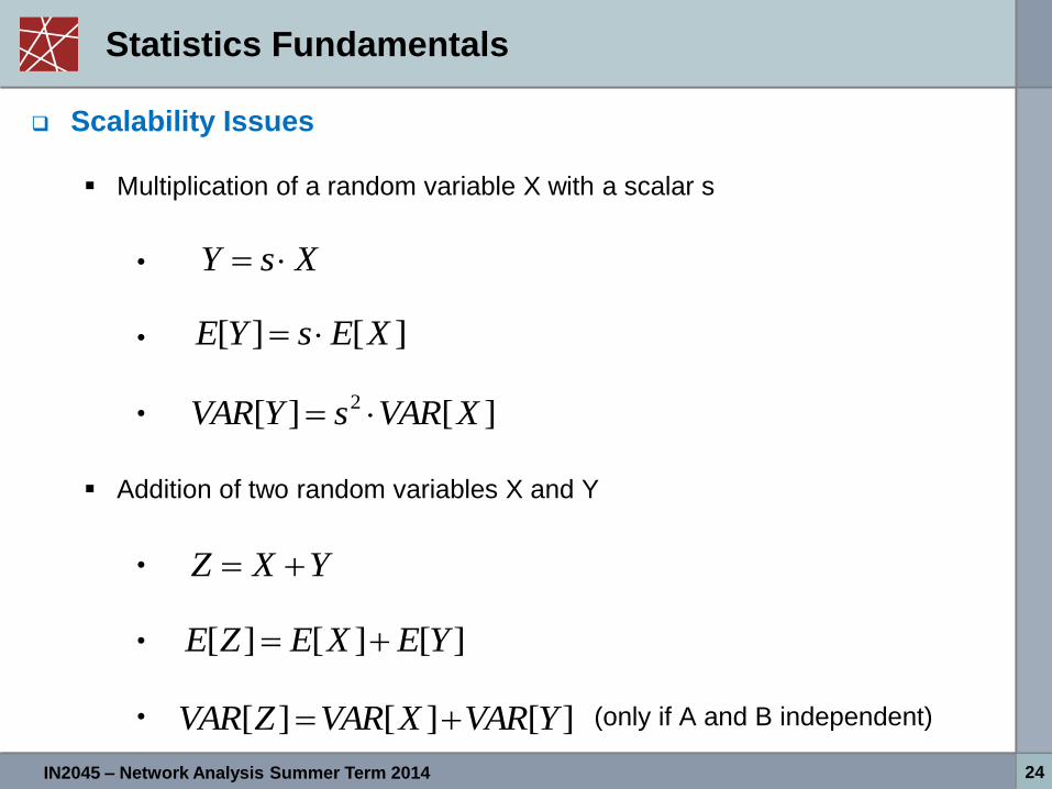
Monty Hall Problem – (also known as the goat problem)
American game show „Let‘s make a deal“ adopted in Germany
„Geh auf Ganze“
Network Security, WS 2008/09, Chapter 9 42 IN2045 – Network Analysis Summer Term 2014 42
Statistics Fundamentals
Game rules:
Behind one door is a price
Behind the other doors is the goat / Zonk (It is assumed that the candidate
is not interested in neither the goat nor the Zonk)
Candidate may choose one door
Game master will open one door after the decision of the candidate and
will offer the candidate the choice to choose a different door.
Should the candidate change his/her decision?

Network Security, WS 2008/09, Chapter 9 43 IN2045 – Network Analysis Summer Term 2014 43
Statistics Fundamentals
Definition: RV Z=i: „Zonk/Goat is behind door i“
P(Z=i)=1/n (Laplace)
Definition: RV C=i: „Candidate has chosen door i“
P(C=i)=1/n (Laplace)
Z an C are independent
P(Z=i ∧ C=i)=P(Z=i)⋅P(C=i)
Definition: ZV O=i: „Door i was opened“
P(O=i|Z=i)=0 „The winning door was not opened“
P(Z=i ∧ O=i) = P(O=i|Z=i)⋅P(Z=i) = 0 (Bayes)
P(Z=i ∧ O≠i) = P(Z=i) – P(Z=i ∧ O=i) = P(Z=i) (Totale Wahrscheinlichkeit)
P(O=i|C=i)=0 „The selected door will NOT be opened“
P(C=i ∧ O=i) = P(O=i|C=i)⋅P(C=i) = 0 (Bayes)
P(C=i ∧ O≠i) = P(C=i) – P(C=i ∧ O=i) = P(C=i) (Totale Wahrscheinlichkeit)

Network Security, WS 2008/09, Chapter 9 44 IN2045 – Network Analysis Summer Term 2014 44
Statistics Fundamentals
)(
))(()|(
iOiCP
iOiCiZPiOiCiZP
Win probability if the player does not change his selection
Win probability if player changes his/her selection
n
n
nn
iZP
iCiZP 1
1
11
)(
)(
2
))((1)|(
n
iOiCiZPiOiCiZP
)2(
1
2
11
nn
n
n
n

Network Security, WS 2008/09, Chapter 9 45 IN2045 – Network Analysis Summer Term 2014 45

Network Security, WS 2008/09, Chapter 9 46 IN2045 – Network Analysis Summer Term 2014 46
Statistics Fundamentals
service
process
arrival
process
buffer, queue
3.4 0.6 1.7 1.6 0.7 0.7 1.3
random numbers
1.7 1.0 3.3 4.0 0.7 ...
service times inter-arrival times
Waiting Queue Theory
rate λ rate μ

Network Security, WS 2008/09, Chapter 9 47 IN2045 – Network Analysis Summer Term 2014 47
Statistics Fundamentals
What are we talking about… and why?
Simple queue model:
Customers arrive at random times
Execution unit serves customers (random duration)
Only one customer at a time; others need to queue
Standard example
Give deeper understanding of important aspects, e.g.
Random distributions (input)
Measurements, time series (output)
…

Network Security, WS 2008/09, Chapter 9 48 IN2045 – Network Analysis Summer Term 2014 48
Statistics Fundamentals
Queuing model: Input and output
Input:
(Inter-)arrival times of customers (usually random)
Job durations (usually random)
Direct output:
Departure times of customers
Indirect output:
Inter-arrival times for departure times of customers
Queue length
Waiting time in the queue
Load of service unit (how often idle, how often working)

Network Security, WS 2008/09, Chapter 9 49 IN2045 – Network Analysis Summer Term 2014 49
Statistics Fundamentals
arrivals
service
durations
3.4 0.6 1.7 1.6 0.7 0.7 1.3
0.7 4.0 3.3 1.0 1.7
event
queue
t
1
2
X(t)
n
W n
B
1 2 5 10
n
Little Theorem

Network Security, WS 2008/09, Chapter 9 50 IN2045 – Network Analysis Summer Term 2014 50
Statistics Fundamentals
Little Theorem
λ : average arrival rate
E[X] : average number of packets in the system
E[T] : average retention time of packets in the system
Arrival Process
Rate λ
E[X]
E[T]
dttXN
TN
TotN
i
i 01
_
)(11
dttXt
Xot
o
0
_
)(1
][_
TEt
NX
o
ot
N
_
___
XT
ott t
N
oo limlim
_
N
i
itt
TN
TTEoo 1
_ 1limlim][
o
oo
t
ott
dttXt
XXE0
_
)(1
limlim][
ot

Network Security, WS 2008/09, Chapter 9 51 IN2045 – Network Analysis Summer Term 2014 51
Statistics Fundamentals
Kendall Notation
GI / GI / n - S
[x]
Number of Servers
Service Time Distribution
Batch Arrival Process
Number of Places in the Queue
Arrival Process
S = 0 Loss/Blocking System
S = Waiting System

Network Security, WS 2008/09, Chapter 9 52 IN2045 – Network Analysis Summer Term 2014 52
Statistics Fundamentals
Queuing Discipline
FIFO / FCFS First In First Out / First Come First Served
LIFO / LCFS Last In First Out / Last Come First Served
SIRO Service In Random
PNPN Priority-based Service
EDF Earliest Deadline First
Distributions
M Markovian Exponential Service Time
D Degenerate Distribution A deterministic service time
Ek Erlang Distribution Erlang k distribution
GI General distribution General independent
Hk Hyper exponential Hyper k distribution

Network Security, WS 2008/09, Chapter 9 53 IN2045 – Network Analysis Summer Term 2014 53
Statistics Fundamentals
System Characteristics
Average customer waiting time
Average processing time of a customer
Average retention time of a customer
Average number of customers in the queue
Customer blocking probability
Utilization of the system / individual processing units

Network Security, WS 2008/09, Chapter 9 54 IN2045 – Network Analysis Summer Term 2014 54
Statistics Fundamentals – Waiting Queue
Questions:
How does the number of service units affect the system?
What impact has a higher variance of the arrival and/or service process on
the performance of the system?
Which system has a higher utilization? One with an unlimited number of
waiting slots or one with a limited number?
Which system has a lower retention time? One with many slow serving
units or on with a single but fast serving unit?
How does the queuing strategy (FIFO, LIFO, EDF) affect the average
waiting time and the waiting time distribution?

Network Security, WS 2008/09, Chapter 9 55 IN2045 – Network Analysis Summer Term 2014 55
Statistics Fundamentals
Exercise
System A: D / D / 1 -
• Arrival rate λ = 1 / s
• Service rate μ = [1;10] / s
System B: M / M / 1 -
• Arrival rate λ = 1 / s
• Service rate μ = [1;10] / s
System C: M / M / 20 -
• Arrival rate λ = 10 / s
• Service rate μ = 1 / s
System D: M / M / 1 -
• Arrival rate λ = 10 / s
• Service rate μ = 20 / s
What is the maximum
(meaningful) utilization of
the system?
Which system performs
better?
What impact does the
utilization have on the
system?
Which system performs
better?
Would you prefer a single
fast processing unit
instead of multiple slow
processing units?

Network Security, WS 2008/09, Chapter 9 56 IN2045 – Network Analysis Summer Term 2014 56
Statistics Fundamentals
Exercise
System E: M / M / 10 -
• Arrival rate λ = 9 / s
• Service rate μ = 1 / s
System F: M / M / 100 -
• Arrival rate λ = 90 / s
• Service rate μ = 1 / s
System G: M / D / 1 -
• Arrival rate λ = 1 / s
• Service rate μ = 1 / 0.7 / s
System H: D / M / 1 -
• Arrival rate λ = 1 / s
• Service rate μ = 1 / 0.7 / s
What is the maximum
(meaningful) utilization of
the system?
Which system performs
better?
Which system performs
better?
Which system has a
shorter avg waiting time?

Network Security, WS 2008/09, Chapter 9 57 IN2045 – Network Analysis Summer Term 2014 57
Statistics Fundamentals
System G: M / D / 1 -
λ = 1 μ = 1 / 0.7 = ~ 1.43
75.0)1( sTP55.0)7.0(1)7.0( sTPsTP
System H: D / M / 1 -

Network Security, WS 2008/09, Chapter 9 60 IN2045 – Network Analysis Summer Term 2014 60
M / M / n -
System of equations
Statistics Fundamentals
Picture taken from Tran-Gia, Analytische Leistungsbewertung verteilter Systeme, p. 98
State Transition Diagram - M / M / n -
,,...,3,2,1),()1( niixiix
,...1),()1( niixnix
0
1)(i
ix
Network Security, WS 2008/09, Chapter 9 61 IN2045 – Network Analysis Summer Term 2014 61
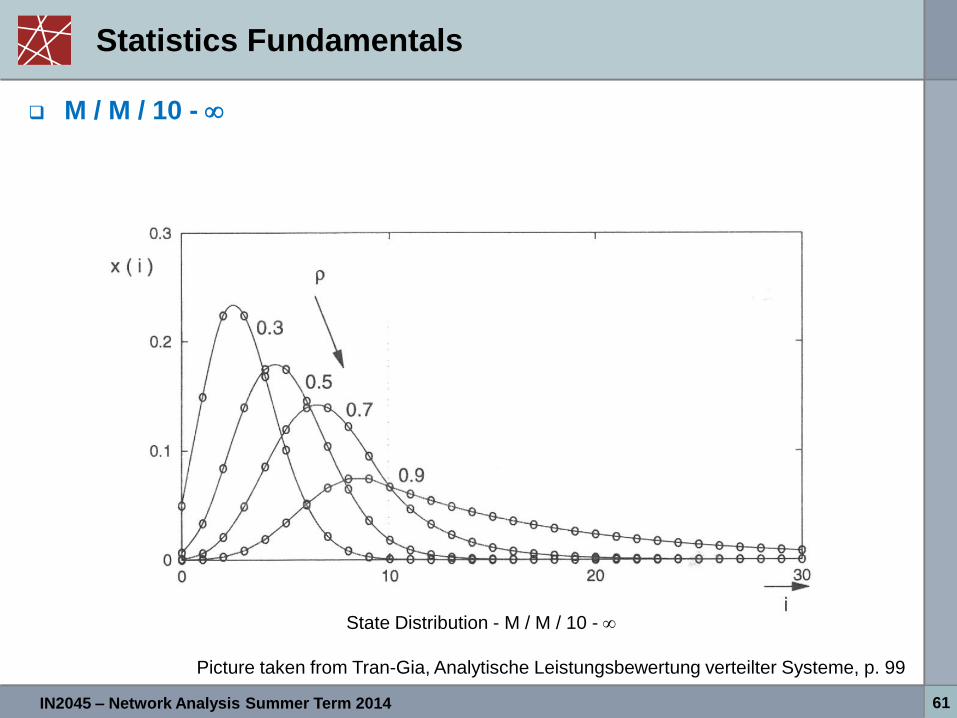
Statistics Fundamentals
M / M / 10 -
Picture taken from Tran-Gia, Analytische Leistungsbewertung verteilter Systeme, p. 99
State Distribution - M / M / 10 -

Network Security, WS 2008/09, Chapter 9 62 IN2045 – Network Analysis Summer Term 2014 62
Statistics Fundamentals
M / M / 10 -
The waiting probability decreases with an increasing number of
processing units (assuming constant utilization)
Utilization Picture taken from Tran-Gia, Analytische Leistungsbewertung verteilter Systeme, p. 100
• n = number of processing
units
• - Waiting probability
W