Embed Size (px)
Citation preview

Network Coding, Multi-Packet Reception, and Feedback:Design Tools for Wireless Broadcast Networks
by
Arman Rezaee
B.S., Electrical EngineeringArizona State University (2009)
MASSACKU F77 i
SEP 2 7 -011
L99FUE
Submitted to the Department of Electrical Engineering and Computer Sciencein Partial Fulfillment of the Requirements for the Degree of
Master of Science in Electrical Engineering and Computer Science
at the
MASSACHUSETTS INSTITUTE OF TECHNOLOGY
September 2011
@ 2011 Massachusetts Institute of Technology. All rights reserved.
Signature of Author .... ............ .... .......... . . . . . . . . . . . . . . . r . .Department of Electrical Engineering and Cc puter Science
September 1, 2011
Certified by ..............
C ertified by ...............................
Muriel M6dardProfessor of Electrical Engineering
Thesis Supervisor
............. ...Linda Zeger
Technical Staff, MIT Lincoln LaboratoryThesis Supervisor
A ccepted by ................................ . .....
Ceie A. KolodziejskiChair, Department Committee on Graduate Students
ARCHIvEs

'2
Network Coding, Multi-Packet Reception, and Feedback:Design Tools for Wireless Broadcast Networks
by
Arman Rezaee
Submitted to the Department of Electrical Engineering and Computer Scienceon September 1, 2011 in partial fulfillment of the
requirements for the degree ofMaster of Science in Electrical Engineering and Computer Science
AbstractIn this thesis, we address the combination of three technologies in wireless broadcast networks:network coding, multi-packet reception (MPR) and feedback. We will primarily discuss the perfor-mance of a single-hop network, both with and without these technologies. A single-hop networkcan be used as a building block for larger and more topologically diverse networks and providesa basis for analyzing the interaction of these mechanisms. Because many applications are inter-ested in speedy transmission of data, we have focused our attention on answering the question ofhow to optimally use these technologies in order to reduce the overall transmission time. Initially,we consider a fully connected network and show that MPR capability of m can reduce the totaltime for a file transfer by as much as a factor of M without network coding. We emphasize that a2two-fold MPR capability will not reduce the total dissemination time without network coding andis thus ineffective. We also show that no gain can be obtained, if network coding is used withoutMPR. However the combination of network coding and MPR can reduce the total transfer timeby as much as a factor of m. We then consider transmission of a file over a broadcast erasurechannel with a potentially large number of receivers. Noting that traditional reliable multicastprotocols suffer from the inevitable feedback implosion associated with servicing a large numberof receivers, we present a novel feedback protocol dubbed SMART, Speeding Multicast by Ac-knowledgment Reduction Technique. The protocol involves an asymptotically optimal predictivemodel which determines a suitable feedback time that assures most receivers have completed thedownload. We also introduce a new single slot feedback mechanism, which enables any numberof receivers to give their feedback simultaneously. We show that scheduling the feedback accord-ing to this predictive model and enhancing the protocol by the single slot mechanism reduces thefeedback traffic as well as transmission of extraneous coded packets, and will provide a good com-pletion time characteristic for all users. We show that counter to conventional wisdom, Quality ofExperience (QoE) of multicast sessions is not sensitive to the number of users, however it is verysensitive to imbalanced effective rate and heterogeneity among users. Furthermore, we show thatSMART performs nearly as well as an omniscient transmitter that requires no feedback.
Thesis Supervisor: Muriel M'dardTitle: Professor of Electrical Engineering
Thesis Supervisor: Linda ZegerTitle: Technical Staff, MIT Lincoln Laboratory

4

Acknowledgments
I would like to thank my advisors, Professor Muriel M6dard, and Dr. Linda Zeger for their support,
enthusiasm, and patience which undoubtedly surpassed my expectations. I feel truly fortunate to
have had the chance to work with such brilliant and talented individuals. Professor Medard has
been extremely understanding and caring through difficult times and I cannot begin to thank her
enough for giving me the opportunity to learn and grow professionally as well as personally.
I would also like to thank my friends and colleagues who have made my MIT experience richer
in every sense of the word. In particular, I would like to thank Flivio du Pin Calmon, Jason Cloud,
Weifei Zeng, Matt Carey, and Georgios Angelopoulos for many wonderful discussions and great
memories. I would also like to thank Soheil Feizi and Ali Parendeh-Gheibi for their insightful
feedback on multitude of topics that I encountered during my research.
I would like to express my deepest gratitude to my parents, brothers, and their beloved families
for their unwavering support and love over the years. It is hard to imagine what I would have done
without them. I am indebted to Houshidar Bahin-aein and Mahshid Rohani, who made their home
and heart open to me and did everything humanly possible to help me in pursuit of my endeavors.
Lastly but foremost, I'd like to dedicate this thesis to my friends in Iran who were denied their
fair share of access to higher education. I am certain that their perseverance and dedication will
soon be paid off.
I acknowledge that various parts of this work are from the papers, porduced in collaboration
with colleagues, and have been presented at various conferences and journals.

6

Contents
1 Introduction 13
1.1 Background and Motivation . . . . . . . . . . . . . . . . . . . . . . . . . . . . . 14
1.2 Main Contribution and Thesis Outline . . . . . . . . . . . . . . . . . . . . . . . . 17
2 Multi-packet Reception and Network Coding 21
2.1 Introduction . . . . . . . . . . . . . . . . . . . . . . . . . . . . . . . . . . . . . . 21
2.2 Network Model and Parameters . . . . . . . . . . . . . . . . . . . . . . . . . . . 23
2.3 Single Packet Reception . . . . . . . . . . . . . . . . . . . . . . . . . . . . . . . 24
2.4 Multi-Packet Reception without Network Coding . . . . . . . . . . . . . . . . . . 26
2.4.1 g m . . .. . .. .. . .. . .. . . . . . .. . . . . . . . . .... . ... . 27
2.4.2 g>m . . .. . .. .. .. .. .. . . . . . .. . . . .. . . . .... ... . 28
2.5 Multi-Packet Reception With Network Coding . . . . . . . . . . . . . . . . . . . . 29
2.5.1 g < m . . . . . . . . . . . . . . . . . . . . . . . . . . . . . . . . . . . . . 29
2.5.2 g>m .. ....... .................. .... ...... .... 31
2.6 Comparison . . . . . . . . . . . . . . . . . . . . . . . . . . . . . . . . . . . . . . 32
2.7 Priority Messages . . . . . . . . . . . . . . . . . . . . . . . . . . . . . . . . . . . 34
2.8 Priority Groups . . . . . . . . . . . . . . . . . . . . . . . . . . . . . . . . . . . . 36
2.8.1 MPR without network coding . . . . . . . . . . . . . . . . . . . . . . . . 37
2.8.2 MPR with network coding . . . . . . . . . . . . . . . . . . . . . . . . . . 38
2.9 Erasures . . . . . . . . . . . . . . . . . . . . . . . . . . . . . . . . . . . . . . . . 40

2.9.1 MPR without Network Coding ..... ........................ 41
2.9.2 MPR with Network Coding ...... ......................... 42
2.9.3 No M PR .. ..... ...... ....... .... . . ..... ... . 43
2.9.4 Discussion . . . . . . . . . .. . .. . . . .. .. . . . . . . . . . . . . . 43
2.10 Networks with non-uniform MPR capability . . . . . . . . . . . . . . . . . . . . . 45
2.10.1 Without Capture Capability . . . . . . . . . . . . . . . . . . . . . . . . . 45
2.10.2 With Capture Capability . . . . . . . . . . . . . . . . . . . . . . . . . . . 47
2.11 Conclusion . . . . . . . . . . . . . . . . . . . . . . . . . . . . . . . . . . . . . . 49
2.12 Appendix A . . . . . . . . . . . . . . . . . . . . . . . . . . . . . . . . . . . . . . 50
2.12.1 Maximal Combinations Strategy . . . . . . . . . . . . . . . . . . . . . . . 50
2.12.2 Ring Structure Strategy . . . . . . . . . . . . . . . . . . . . . . . . . . . . 50
3 SMART:
Speeding Multicast by Acknowledgement Reduction Technique 53
3.1 Introduction . . . . . . . . . . . . . . . . . . . . . . . . . . . . . . . . . . . . . . 53
3.2 Network Model and Auxiliary Concepts . . . . . . . . . . . . . . . . . . . . . . . 55
3.2.1 Network Model and Problem Setup . . . . . . . . . . . . . . . . . . . . . 55
3.2.2 Method of Types . . . . . . . . . . . . . . . . . . . . . . . . . . . . . . . 56
3.3 SMART over Networks with Homogeneous Links . . . . . . . . . . . . . . . . . . 61
3.3.1 Characterization of Ni . . . . . . . . . . . . . . . . . . . . . . . . . . . . 67
3.3.2 Characterization of K1 . . . . . . . . . . . . . . . . . . . . . . . . . . . . 69
3.4 SMART over Networks with Heterogeneous Links . . . . . . . . . . . . . . . . . 69
3.4.1 Networks with Two Heterogeneous Links . . . . . . . . . . . . . . . . . . 70
3.4.2 General Single-Hop Networks . . . . . . . . . . . . . . . . . . . . . . . . 74
3.5 SMART in a Continuous Transmission Model . . . . . . . . . . . . . . . . . . . . 75
3.6 Operational Aspects . . . . . . . . . . . . . . . . . . . . . . . . . . . . . . . . . . 78
3.6.1 Mechanism for Single-slot Feedback . . . . . . . . . . . . . . . . . . . . . 78
3.6.2 Robustness of SMART . . . . . . . . . . . . . . . . . . . . . . . . . . . . 80

3.6.3 Performance Comparison . . . . . . . . . . . . . . . . . . . . . . . . . . . 81
3.7 Conclusion . . . . . . . . . . . . . . . . . . . . . . . . . . . . . . . . . . . . . . 84
4 Conclusion and Future Work 85

List of Figures
2.1 Tot, as a function of m for different values of g and k = 1. Solid lines denote use
of network coding and dashed lines are for the case without coding. . . . . . . . . 33
2.2 Tot, as a function of n for different ratios of g/n when m = 4 and k = 1. Solid
lines denote use of network coding and dashed lines are for the case without coding. 34
2.3 Tot,/k as a function of g for different values of m. . . . . . . . . . . . . . . . . . . 35
2.4 Tott as a function of k for different values of m when n > 9 and g = 5. . . . . . . . 36
2.5 Tt/k as a function of g for groups of equal size. . . . . . . . . . . . . . . . . . . 39
2.6 Tott/k as a function of g for groups of unequal size. . . . . . . . . . . . . . . . . . 40
2.7 Comparison of CDFs of total delivery time R 1 with respect to MPR and network
coding capabilities. Network parameters are: n = 30, g = m = 2, k = 5, qO = 0.2. 44
3.1 Calculation E [Sii.(t, n, Q)] from #8n (t, n, 1, Q) . . . . . . . . . . . . . . . . . 59
3.2 Calculating E [T I (n, k, Q)] from 1 - #ln(t, n, k, Q) . . . . . . . . . . . . . . . 60
3.3 Completion probability as a function of t for different values of qo. Computed from
(3.12) . . . . . . . . . . . . . . . . . . . . . . . . . . . . . . . . . . . . . . . . . 62
3.4 Completion probability as a function of t for varying k and n when qO = 0.1. Com-
puted from (3.12) . . . . . . . . . . . . . . . . . . . . . . . . . . . . . . . . . . . 63
3.5 Pictorial depiction of SMART's operation . . . . . . . . . . . . . . . . . . . . . . 63
3.6 Computed values of T1 and simulated values of Tot for varying network and file
sizes with qo = 0.1 . . . . . . . . . . . . . . . . . . . . . . . . . . . . . . . . . . 67
3.7 Sample network with n = 8, and M = 4 . . . . . . . . . . . . . . . . . . . . . . . 70

3.8 a) #(t) for a network of 1000 receivers, all of which have access to both links. b)
#6(t) for a network where 999 nodes have access to both links but 1 node has a
single link connection. (Both figures are computed from eq. (3.28)) . . . . . . . . 73
3.9 Calculating t* from the (' function. . . . . . . . . . . . . . . . . . . . . . . . 76
3.10 The number of nodes n that can be accommodated for a given transmission time
t. The figure was computed according to (3.37) with k = 100 packets and q0 =
0.1. An example of how the time t* (* n) can be obtained from these curves is
illustrated by the dashed lines for the case of #* = 0.9 and n = 1000. . . . . . . . . 78
3.11 Simulation results depicting the performance of SMART, the theoretical bound
obtained from a genie based protocol, and a wireless representation of NORM. . . 82
3.12 Feedback times for NORM vs. SMART for n = 10000, k = 100, and qo = 0.3.
The number above each blue bar indicates the number of slots devoted to NACKs
at that cycle and red bars denote the end of transmissions. . . . . . . . . . . . . . . 83

List of Tables
2.1 Transmission schedule of a network with n = 8, g = 5, and m = 1 . . . . . . . . . 25
2.2 Transmission schedule of a network with n = 8, g = 5, and m = 2 without
network coding . . . . . . . . . . . . . . . . . . . . . . . . . . . . . . . . . . . . 27
2.3 Transmission schedule of a network with n = 8, g = 5, and m = 2 with network
coding . . . . . . . . . . . . . . . . . . . . . . . . . . . . . . . . . . . . . . . . . 30
Chapter 1
Introduction
The advent of digital communications in the latter half of the twentieth century and its broad set of
applications have brought about a new age, the information age. What is truly astonishing about
this era is the rapid technological advances that have uplifted modern life from an industrial setting.
At the forefront of this transformation is the wireless revolution, which has brought communities
closer together and has made it possible for everyone to stay in touch and quench their thirst for
globally created content.
An important feature of the information age is the speed at which information is transferred and
the rapid, and rather unusual, demand for data and content. This has unleashed an unprecedented
effort in design and implementation of physical transmission media such as wave guides and fiber
optics. These advances were made possible as the research community has developed ever-more
accurate models of natural phenomena such as fading and interference in wireless channels, or
optical coherence in fibers. There has also been a great reconsideration of multi-objective commu-
nication protocols. Fairness, priority, delay sensitivity and reliability are examples of objectives
that are vital to performance of communication systems in this new environment.
Wireless networks and communication systems are now an important part of our daily lives
and activities. It is hard to imagine a day without cell phones and instantaneous access to email
or social network accounts. The rapid growth of the global market has created a set of devices

inherently different in design and purpose, which need to work together in order to be effective and
useful. Design and maintenance of such heterogeneous networks, and most importantly, a seamless
integration of different technologies, have become the challenges that face many engineers and
scientists. For years, new technologies have been added to engineers' toolboxes without a clear
road map for their integration. Noting that performance of any device is ultimately dependent
on wise integration of such technologies, we would like to study a few of these technologies and
propose solutions for their joint utilization.
In this thesis, we address the combination of three technologies in wireless networks: network
coding, multi-packet reception and feedback. We will primarily discuss the performance of a
single-hop network, both with and without these technologies. A single-hop network can be used
as a building block for larger and more topologically diverse networks and will provide a basis for
analyzing the interaction of these mechanisms. Because many applications are interested in speedy
transmission of data, we will focus our attention on answering the question of how to optimally
use these technologies in order to reduce the overall transmission time.
1.1 Background and Motivation
The research endeavors of Claude Shannon, one of the greatest mathematicians of the twentieth
century, culminated in a groundbreaking paper in 1948 titled "A Mathematical Theory of Commu-
nication" [1]. Despite many failed attempts by his predecessors, Shannon was the first to method-
ically analyze a complete communication system in terms of its components and provide insight
into their inherent complexity, ability, and limitations. Shannon introduced new ideas such as en-
tropy, mutual information, and even the term "bit" to quantify and measure information in a natural
way. He also defined a quantity, known as channel capacity, which is the maximum amount of in-
formation that can be reliably transmitted over a noisy channel. His findings set the stage for a
challenge that has lasted more than half a century as mathematicians and engineers propose dif-
ferent schemes to achieve the channel capacity. The idea has been to send extra information (bits)

to compensate for the losses introduced by the channel. In information theoretic terms, we use
"channel coding" to protect the transmitted data against noise. Many coding schemes have been
developed over the years to address this problem: Convolutional codes, Reed-Solomon codes,
Turbo codes, and Low-Density Parity Check (LDPC) codes to name a few.
A subset of the aforementioned codes, for example LDPC codes, are known to be capacity-
achieving in the sense that they enable digital communication at the maximum theoretical limit
across a point-to-point channel. Unfortunately, all these codes are designed for point-to-point
communication and do not extend to general networks. The problem of communicating across
general networks is deeper than the lack of operational codes. In fact, we do not know the capacity
of a general network, and the field of network information theory has yet to solve the problem for
the simplest of networks, namely a three-node relay channel. Despite the challenges that we face in
understanding the complex nature of networks, we have been able to operate large communication
networks such as the Internet that connects billions of users.
Operation of large heterogeneous data networks is governed by a set of protocols that dic-
tate the behavior of each node within the network. Traditionally, Internet content providers and
network operators have used routing as a means by which intermediate nodes within a network
forward the data to the destination nodes. Consider a broadcast scenario whereby a single server
is streaming a sporting event to a potentially large set of receivers across a network. The current
routing mechanisms will establish distinct unicast sessions between the source and each receiver,
and the sessions will operate independently. In other words, they exclude the possibility of co-
operation amongst the receivers and do not allow intermediate nodes to do anything but forward
the packets. The question is whether there are robust solutions that can outperform routing, and if
there are such solutions can we implement them in a distributed manner.
Ahlswede et. al. [2] introduced the idea of network coding and noted that, in a packetized
data network, we should not restrict intermediate nodes to only forwarding their incoming pack-
ets, but rather allow them to operate on the incoming packets. In other words, the intermediate
nodes should mix the incoming data in an appropriate manner and then forward the mix on their

output links. In particular, Ahlswede et. al. showed the sub-optimality of routing in multicast and
proved that network coding is capacity-achieving for simple multicast. This information theoretic
approach did not specify an implementable operation for intermediate nodes until further research
by Li et. al. [3] showed that there exists a scalar linear solution for any solvable multicast network,
if we consider a sufficiently large finite field. Koetter et. al. [4] provided an algebraic framework
for network coding and showed that simple codes can be constructed to achieve the multicast ca-
pacity of a general network. Finally, Ho et. al. [5] introduced random linear network coding as
a feasible distributed mechanism that achieves the multicast capacity of networks. With random
linear network coding, an intermediate node constructs its output as a linear combination of the
input packets. The coefficients of the linear combination are chosen at random from a sufficiently
large finite field.
Network coding has been implemented on many platforms [6, 7, 8, 9] and it has proven to be
an important tool in design of future networks. There are still unanswered questions about net-
work coding in wireless domains especially because of multi-user interference. New techniques
such as orthogonal frequency-division multiplexing (OFDM), orthogonal frequency-division mul-
tiple access (OFDMA), and direct sequence code-division multiple access (DS-CDMA) can allow
a node to receive multiple packets simultaneously, thus giving the perfect opportunity for an in-
termediate node to combine packets from different streams. The ability to simultaneously receive
packets from multiple sources is referred to as multi-packet reception (MPR) capability. Chapter
2 analyzes the combined effects of network coding and MPR and explores the advantages and
drawbacks of their combination under different scenarios.
Another important issue in communication networks is reliability. Applications employ auto-
matic repeat requests (ARQ), forward error correction (FEC), or simple feedback to achieve certain
reliability criteria. Unfortunately, reliability criteria are highly dependent on the network topology,
data content, and the application in mind. For example, bulk data transfer requires very high relia-
bility with almost no delay constraints while video conferencing is very sensitive to delay (because
of human interaction) but not very reliable. Most of these applications use feedback to confirm the

successful reception of their content to the receivers. In unicast sessions, feedback has been widely
used and many congestion control protocols, such as TCP, depend on it for their operation. On the
other hand, when multicasting to a large set of receivers the sheer amount of feedback can over-
whelm the network and attention should be paid to the feedback traffic behavior. Many protocols
[10, 11, 12, 13] try to address this issue but have been unsuccessful in providing a ubiquitous so-
lution. Chapter 3 will develop a multicast protocol, SMART, that achieves the maximum possible
throughput of a multicast network. The protocol is versatile and can be used in wireless as well as
wired networks. It should be noted that network coding acts as an enabler for this protocol, and we
will show the advantages of this scheme for a diverse set of situations.
1.2 Main Contribution and Thesis Outline
This section will provide an overview of the thesis and present the underlying logical links that con-
nect the ideas developed throughout the rest of the thesis. The topics discussed in the remainder of
this thesis are broken into two distinct parts, chapters 2 and 3 respectively. Chapter 2 discusses the
combination of network coding and multi-packet reception (MPR) in a fully connected network,
and Chapter 3 introduces a new approach in designing reliable multicast protocols with minimal
feedback. The overarching theme in both chapters is development of strategies that reduce the
total transmission time required to send a file (or a set of files) to a set of receivers. The main
contributions of this thesis can be stated as:
1. We show that multi-packet reception of 2 will not reduce the total transmission time in a
fully connected network, unless accompanied by network coding.
2. We show that network coding can substitute for some degree of MPR, and will reduce the
total transmission time by a factor of approximately 2.
3. We develop an asymptotically optimal predictive model for multicast that will minimize the
need for feedback.

4. We introduce a mechanism for wireless broadcast systems, so that the base station can ac-
quire feedback from all receivers in a single time slot.
5. We show that a combination of single slot feedback, and the predictive model will allow a
multicast protocol to perform close to an omniscient transmitter that knows the state of every
link and every receiver at all times.
The network models discussed in each chapter differ slightly and will be explained thoroughly
at the beginning of each chapter.
Chapter 2 is comprised of ten main sections. The chapter starts with a detailed explanation
of the network model and parameters and will provide insight into some of the assumptions used
for the chosen model. It will characterize optimal transmission strategies for single-packet re-
ception as well as multi-packet reception with and without network coding. Simulation results
will be presented to compare the performance of the system under all aforementioned conditions.
The analysis will then be extended to networks that accommodate priority messages and priority
nodes. It will then discuss networks with varying MPR capabilities and the challenges involved in
upgrading the MPR capability of the nodes within a network. We will then generalize the results
to networks with erasures and present heuristics on the performance of the network.
Chapter 3, is comprised of six main sections. In this chapter, we present a novel feedback
protocol (SMART) for wireless broadcast networks that use linear network coding. We propose a
predictive model to minimize feedback as well as extraneous data transmissions by the source. We
show that with our NACK-based protocol, few receivers (if any) will be in need of retransmissions
by the first feedback and thus few nodes will participate in the feedback. This result is particularly
important when multicasting to a large number of receivers, since full participation of the receivers
in the feedback can overwhelm the network and have catastrophic effects. We use the method of
types to provide a lower bound for the expected total transmission time and use simulations to show
that our protocol operates close to this lower bound. We show empirically that reliable multicast
can provide a good completion time characteristic for all users, if the initial feedback is delayed
until the expected download completion time.

We show that counter to conventional wisdom, quality of experience (QoE) of multicast ses-
sions is not sensitive to the number of users, however it is very sensitive to imbalanced effective
rate and heterogeneity among users. We demonstrate that SMART's algorithmic simplicity enables
multicast transmissions that on average take fewer than 2 feedback rounds to complete. We show
the favorable scalability of our technique with the number of users, which enables reliable qual-
ity of experience. Furthermore, we show that SMART performs nearly as well as an omniscient
transmitter that requires no feedback.
In Chapter 4, we summarize the contributions of this thesis, and present possible topics to be
considered in future works.

20

Chapter 2
Multi-packet Reception and Network
Coding
2.1 Introduction
In networks, multi-user interference is an important limitation. In order to alleviate it, the use
of multi-packet reception (MPR) has been proposed [14], [15]. MPR may be implemented in
a variety of ways through use of different conventional physical layer channels, ranging from
orthogonal signaling schemes such as OFDM to spread spectrum techniques such as frequency
hopping or DS-CDMA. In addition, MPR could be implemented with a new technique we propose
that appends both a preamble and a postamble to each packet. The use of both a preamble and
postamble could allow both the leading and trailing packets in a collision to be identified, and
thereby enable potential recovery of both packets at the receiver, for example, through interference
cancellation. Both the conventional and new techniques would allow a limited number of packets
to be simultaneously received at a node with MPR capability. In this chapter we analyze the effects
on network performance of a range of MPR capabilities, without restricting ourselves to specific
physical layer implementations.
Multi-packet reception can help when used with wireless MAC protocols (e.g. ALOHA), in

which conventional models consider the transmission of multiple packets to be a collision and
the throughput can be optimized through different back-off mechanisms [16]. The stability and
delay of ALOHA with MPR have been studied in [17] and [18] for finite and infinite-user slotted
channels. There has been a renewed interest in capture schemes as explained in [19], [20], and
[21], the simplest form of which can be used to capture the packet from the signal that has higher
energy at the receiver.
It has been shown, in [2] and [5], that network coding can be used to improve throughput
by allowing mixing of data at intermediate nodes in a network. If network coding and MPR are
used together, we expect a higher throughput because MPR at a node enables combination of
diverse packets which can be coded together and consequently, each transmission can on average
disseminate more information to the network. The main focus of this chapter is to show when and
where we should combine network coding with multi-packet reception to improve performance.
The rest of this chapter is organized as follows: In Section 2.2, the network model and pa-
rameters are introduced. In Section 2.3, we characterize single-packet reception. In Section 2.4,
multi-packet reception without network coding is described. In Section 2.5, we present the gains
associated with the combination of network coding and multi-packet reception. In Section 2.6, we
present a brief comparison of the results for practical networks. In Sections 2.7, and 2.8 we will
extend the previous results to networks that accommodate priority messages and priority nodes
respectively. In Section 2.9, we introduce erasures to the network model and provide heuristics
about the delay performance of the network. In Section 2.10, we discuss networks with nodes of
varying MPR capabilities. Finally, we provide a summary and concluding remarks in Section 2.11.
Appendix A, describes two schemes that can be used to optimally transmit packets from a group
of g nodes given a specific MPR capability.
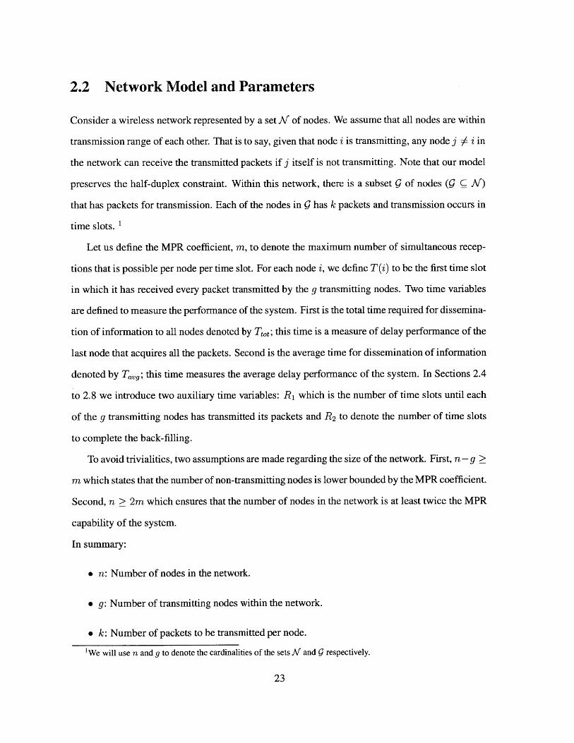
2.2 Network Model and Parameters
Consider a wireless network represented by a set A' of nodes. We assume that all nodes are within
transmission range of each other. That is to say, given that node i is transmitting, any node j # i in
the network can receive the transmitted packets if j itself is not transmitting. Note that our model
preserves the half-duplex constraint. Within this network, there is a subset 9 of nodes (9 C K)
that has packets for transmission. Each of the nodes in 9 has k packets and transmission occurs in
time slots. 1
Let us define the MPR coefficient, m, to denote the maximum number of simultaneous recep-
tions that is possible per node per time slot. For each node i, we define T(i) to be the first time slot
in which it has received every packet transmitted by the g transmitting nodes. Two time variables
are defined to measure the performance of the system. First is the total time required for dissemina-
tion of information to all nodes denoted by Tet,; this time is a measure of delay performance of the
last node that acquires all the packets. Second is the average time for dissemination of information
denoted by Tavg; this time measures the average delay performance of the system. In Sections 2.4
to 2.8 we introduce two auxiliary time variables: R 1 which is the number of time slots until each
of the g transmitting nodes has transmitted its packets and R 2 to denote the number of time slots
to complete the back-filling.
To avoid trivialities, two assumptions are made regarding the size of the network. First, n - g >
m which states that the number of non-transmitting nodes is lower bounded by the MPR coefficient.
Second, n > 2m which ensures that the number of nodes in the network is at least twice the MPR
capability of the system.
In summary:
" n: Number of nodes in the network.
" g: Number of transmitting nodes within the network.
" k: Number of packets to be transmitted per node.
'We will use n and g to denote the cardinalities of the sets K and g respectively.

* m: Number of possible receptions per node per time slot.
" T(i): The first time slot in which node i has received every packet.
* R 1 : Number of time slots until each of the g transmitting nodes has transmitted its packets.
(Round 1)
" R 2 : Number of time slots to complete the back-filling process. (Round 2)
" T 0t&: Total time required for dissemination of information (in time slots).
" Tavg: Average time for a node to receive the last packet of the transmitted information (in
time slots).
" NC, NC : Denote network coding, or lack of it, respectively.
" MPR, MPR : Denote multi-packet reception, or lack of it, respectively.
n - g > m
* n > 2m
2.3 Single Packet Reception
Since m = 1, all transmitting nodes will take turns transmitting their packet. Thus for k = 1:
TMPR
More generally, if each of the g transmitting nodes has k > 1 packets to transmit, the total time
will be increased by a factor of k and:
= gkTot (2.1)

Consider the case where each of the g transmitting nodes successively transmits all of its k packets.
It can be seen that the last transmitting node will have every packet after (g - 1) k transmissions
and every other node will have it after gk transmissions. Thus:
MPR I
Tavg E T(i)i=1
(2.2)
Table 2.1 demonstrates how a typical transmission takes place when g = 5, and n = 8 without
MPR. Each node is denoted by a letter, A through H, and time slots are enumerated by ti to
t5. During each time slot, the transmitting node is explicitly marked with an arrow. For example
XA -+, shows that node A transmitted during ti and its packet was received by every other node
during the same time slot as denoted by XA in the other rows.
Node (i) t1 t2 J 3 t 4 t T(i)
A XA-- XB Xc XD XE 5
B XA XB -+ Xc XD XE 5
C XA XB Xc-+ XD XE 5
D XA XB XC XD-* XE 5
E XA XB Xc XD XE-* 4
F XA XB Xc XD XE 5
G XA XB Xc XD XE 5
H XA XB XC XD XE 5
Table 2.1: Transmission schedule of a network with n = 8, g = 5, and m = 1
Note that since MPR is not present, coding cannot help. In other words, if each node codes its
packets before transmission, there will be no reduction in the total transmission time or the average
transmission time. Hence:
MPR,NC
Tavg
MPRNC
tt-
MPR,NC
avg
MPR,NC
Tot
=g k - 3

2.4 Multi-Packet Reception without Network Coding
Consider g transmitting nodes, each with one packet to be distributed to every other node. Since
receivers are limited by m receptions per time slot, the set of transmitting nodes is partitioned into
groups of m nodes such that all nodes in a given group can transmit simultaneously. If g is not a
multiple of m, the last group will have g mod m nodes. Let R1 denote the first transmission round,
within which all transmitting nodes complete the transmission of their files. Thus R1 is the number
of time slots it takes until each of the g transmitting nodes has transmitted its packet. There will be
[I1 such groups, thus:
R1,
Because of half-duplex constraints, the g transmitting nodes need to be back-filled. Note that
transmissions occur in distinct groups of m nodes, and each transmitting node has missed a maxi-
mum of m -1 packets during its transmission slot. Since n - g > m in our model, the network will
back-fill the previously defined groups consecutively by utilizing m of the non-transmitting nodes.
Each group can be back-filled in one time slot and back-filling will take the same number of slots
as R 1. Let R2 denote the second transmission round within which back-filling is completed:
R 2 = []u(g-1)
where u(g) is the unit step function defined as:
U(g)= :g<;
1 :g> 0
Table 2.2 shows a sample transmission schedule for n = 8, g = 5, and m = 2. We note that
this sample does not fully utilize the MPR since node E transmits alone. In contrast, our scheduling
discussed in Section 2.4.2 below more fully utilizes MPR.

Node (i) t1 t2 t3 t4 t T(i)
A XA-4 XC, XD XE XB 4
B XB-+ XC,XD XE XA 4
C XA,XB XC-+ XE XD 5
D XA,XB XD-+ XE Xc 5
E XA,XB XC,XD XE -+ 2
F XA,XB XC,XD XE XA-* Xc-4 3
G XA,XB XC,XD XE XB-+ XD-- 3
H XA,XB XC,XD XE 3
Table 2.2: Transmission schedule of a network with n = 8, g = 5, and m = 2 without networkcoding
Now consider the case where each transmitting node has k packets. We will present the results for
two separate cases, namely for g < m and g > m.
2.4.1 g < m
When the number of transmitting nodes is less than the MPR coefficient, we are not able to fully
utilize the MPR capability of the system, and the initial transmissions will occur in groups of g
nodes per time slot and:
R 1 = k
As discussed previously, n - g > m and we will backfill the g transmitting nodes by m of the
non-transmitting nodes. Thus:
R2 = [ u(g - 1)m

Thus, the total completion time is:
MPR,NC
Tot =R1+2
= k+ - u(g - 1) (2.3)
The average completion time can be upper bounded by noting that the n - g non-transmitting
nodes will have all the data by R 1 and the g transmitting nodes will have every packet in at most
R 1 + R 2 time slots. Thus:
T MPR,NC (n - g)R1 + g(Ri + R 2 )
gavg '
< k + g]u(g-) (2.4)n Im
2.4.2 g > m
In this case, the optimal strategy is to transmit m new packets in each time slot. There are multiple
ways to ensure that m new packets are transmitted in each time slot and we have outlined two of
them in Appendix A. For the remainder of this chapter, we will consider the Ring Structure method
which completes the transmission of all packets in gk/m time slots with an added constraint that
k should be a multiple of m. Notice that we have reached the information theoretic limit on how
fast we can send gk packets. Thus:
gkR1 = - (2.5)
Recall that the g transmitting nodes need to be back-filled because of half-duplex constraints.
Since the m-node transmitting groups during R1 are distinct and known to other nodes, we can
back-fill them in the order that they transmitted. Let R 2 denote the back-filling time:
R2 = $k (2.6)m

Thus, the total completion time is:
MPRNC = Rgk) (2.7)Tot R1 + R2 = 2 (2.7)
The average completion time can be upper bounded following the same argument used in 2.4.1.
Thus:
T M PRIC < (n - g)R1 + g(R1 + R 2)Tavg -
< -k 1 +9- (2.8)
2.5 Multi-Packet Reception With Network Coding
Following the model presented in Section 2.4, we will introduce network coding as an instrument
to reduce the total transmission time. We present a strategy that utilizes network coding only in
back-filling. Table 2.3 illustrates an example in detail; this example, like that in Table 2.2, is
suboptimal since node E transmits alone and hence the MPR capability is not fully leveraged.
However, our scheduling in Section 2.5.2 more fully utilizes the MPR. Coefficients ai through a5
are used as coding coefficients and are chosen according to the size of the required finite field. As
before, let us analyze the problem separately for g < m and g > m.
2.5.1 g < m
Since we only use network coding in backfilling, R 1 is the same as the case of MPR with no
network coding:
R1, k
Recall that n - g > m, so we can find at least m nodes that did not participate in any of the
previous transmissions and have received each of the gk transmitted packets. The back-filling is

Node (i) ti t2 t3 t4 T(i)
A XA-- XC,XD XE XE 4
B XB-- XC,XD XE XA 4
C XA,XB XC -4 XE XD 4
D XA,XB XD -+ XE Xc 4
E XA,XB XC,XD XE -+ 2
a1XA + a2XB+F XA,XB XC,XD XE a3XC +a4XD+ 3
a5XE-+
G XA,XB XC,XD XE 3
H XA,XB XC,XD XE 3
Table 2.3: Transmission schedule of a network with n = 8, g = 5, and m 2 with networkcoding
accomplished by having each of these m nodes transmit a linear combination of all the packets that
it has received so far. Every time these m nodes transmit, m independent coded packets are sent
out and, as a result, the original g transmitting nodes will get m new degrees of freedom in each
time slot and back-filling will be completed in [(g - 1)k/ml time slots. Thus:
R2 = [ ku(g -)
The total transmission time for this strategy is:
MPR,NCTot = R1 + R2
= k + I M U(g-1) (2.9)
To calculate the average completion time, recall that all non-transmitting nodes will have every
packet by R1 and the g transmitting nodes will have the data after R1 + R 2 time slots. Thus:
TMPR,NCavg(n - g)R1+ g(RI + R 2 )
k+[(g -)ku(gn m
(2.10)

2.5.2 g > m
As in Section 2.4.2, let us assume that k is a multiple of m and use the Ring Structure to transmit
the k packets from each transmitting node. As a result, R 1 is not affected by network coding and:
gkm
During each transmission, exactly m nodes transmitted simultaneously and any given node
within a transmitting group was unable to receive the packets from the other m - 1 nodes. Since
each node transmitted k packets, it is missing (m - 1)k packets in total. Following the same
reasoning used in Section 2.5.1, the back-filling will be completed in (m - 1)k/m time slots.
Thus:
R2= (m -1)km
Thus, the total completion time is:
MPR,NC
k= -(g + m-1) (2.11)
The average completion time can be calculated as:
T MPR,NC _ (n - g)R1 + g(Ri + R 2)avg ~
= kI - 1 (2.12)
This strategy demonstrates how network coding can be used with MPR to reduce the total and
average transmission times.

2.6 Comparison
In practical networks the number of transmitting nodes is usually much greater than the MPR
capability of the system, hence we will compare the results of Sections 2.3, 2.4, and 2.5 for the
case where g > m. Let us revisit the results when each transmitting node has k packets.
Without MPR:
MPR,NC MPRNCTo gk (2.13)
MPR,NC MPRNC kTavg = Tavg nk-(.4
When MPR of m is used without network coding:
TPRNC =2 ( ) (2.15)
MPR,N < k +9Tavg < (2.16)
ma n
When MPR is complemented with network coding:
MPR,NC-) (2.17)
MPR,NC gk (1 m 1) (2.18)m n
Comparing (2.13) and (2.15), we can see that MPR reduces Tt by a factor of m/2. Note that
when m = 2, the total transmission time remains unchanged. This is depicted in Fig. 2.1 where
lack of network coding is represented by dashed lines. Notice that the dashed lines do not change
between m = 1 and 2. We will later compare this result with the case that combines MPR with
network coding.
To see the advantage of network coding, compare (2.15) to (2.17). The total transmission time
is reduced by a factor of 2g/(g + m - 1) which becomes arbitrarily close to two with increasing
g. Let us revisit Fig. 2.1. An ellipse in the figure points out the close proximity of two lines:

-a--- g = 50 with coding
45 - - ---- g = 33 with coding
D-- g = 25 with coding
40 ...... ........ g = 0withoutcoding
- %- g = 33 without coding
35 --- - - - - - -.-- g = 25 without coding
c: 30 -
21 - 5...
%
10--
Figure 2.1: Trot as a function of m for different values of g and k = 1. Solid lines denote use ofnetwork coding and dashed lines are for the case without coding.
one representig g = 50 with coding and the other g 25 without coding. Coding yields the
same total dissemination time as a network with no coding and only half the traffic. Note that if
network coding is used, we can reduce the total transmission time even when m = 2, which was
not achievable without network coding. While Fig. 2.1 presents the value of Tot for k = 1 packet
per transmitting node, if k > 1 and k satisfies the integrality constraint discussed in Sections 2.4
and 2.5, the value of Tt shown in this figure would be multiplied by k. We will follow the same
approach in calculations of Tot, in Fig. 2.2 and Fig. 2.3.
In Fig. 2.2, we show that when m is fixed, Tot~ grows linearly with the number of nodes if
the ratio g/n is kept constant. As shown in the figure, the total transmission time of a network
with g = [n/2] transmitting nodes that uses network coding is only slightly higher than that of a
network with g = [n/4] transmitting nodes that does not use coding.
Fig. 2.3 shows that for a given value of m, the total time Tot, increases linearly with the number
of transmitting nodes g. It is interesting to note that the lines in the figure cross one another when
g E [1, 4]. This occurs because g < m in this range, and the behavior is governed by equations
(2.3) and (2.9) where we have assumed that k is divisible by m to allow scalability for the results.
If the traffic comes from a fixed number of nodes g, the total transmission time Tot, will not be

25 . ....
-a- g - Fn/21 with coding
-O- g - rIn/31 with cod ing
-g>- gr n/41 with coding- 0- g - rn/21 without coding
- 0- g-.fn/31without coding
-rV-g- n/41 without coding
5 .
ga-d[n/21 with codingg F-In41 without coding
020 30 40 50 60 70 80 90 100
Number of Nodes (n)
Figure 2.2: Trot as a function of ni for different ratios of g/n when m= 4 and k = 1. Solid linesdenote use of network coding and dashed lines are for the case without coding.
affected by an increase in n.
Finally, Fig. 2.4 illustrates how the number of packets k at each transmitting node affects Trot
for a network with n ;> 9 and g = 5. Notice the similarity between Fig. 2.3 and Fig. 2.4. In
essence Teot increases linearly with the number of packets k. Again, notice that total transmission
time of m= 2 with coding and m = 4 without coding are close to each other. The amount of time
saved by adding network coding to a fixed level m of MPR is seen to increase with the number of
packets k. The small discontinuities seen on each line are caused by the integrality constraint on
k.
2.7 Priority Messages
Let us generalize the results of previous sections to a network that can accommodate L priority
levels among the messages. Consider the case in which each of the g transmitting nodes has a total
of k packets such that a portion kg of the packets have ith level priority (i E [1, L]). Let ki and kL
denote the highest and lowest priority levels respectively. We assume that g;> m, and the number

m h u ft codng' .
m = 3 with c~ g m wf h coding-. .
1 2 3 4 5 6 7 8 9 10 11 12 13 14 15Number of transmitting nodes (g)
Figure 2.3: Tt ,/k as a function of g for different values of m.
ki of messages with zth level priority is a multiple of m. The g transmitting nodes will transmit
their ki highest priority packets, be back-filled immediately, and then move on to the lower priority
messages. Let 'f'i denote the time slot at which transmission of the ith level priority messages is
completed. Then using equations (2.7) and (2.11) we obtain:
-MP,' C 2 (2.19)j=1
-M"PR,NC g+TtM PRtN - (Y r 1 j (2.20)
j=1
and the total transmission time of all k packets are:
L
L=tO 2To' -- ( 21 (2.22)
i=1
It is interesting to note that there is no penalty in having L priority levels for messages as
long as the number of packets in each priority level ki meets the integrality constraint (i.e. ki is a

S2500 mzncan,-
2 0 0 0 -...- .-. . .... . ..-. . ..-. .. .. -.. .. .-..-.-.-
1500 - -
100 100 0 0 0 60 70 80 90 10
mm - 4 wthout coding
m -3 with codig|50 0 - . . . .. .. ... . .... ... .. . ..
00 100 200 300 400 500 600 700 800 900 1000
Number of packets (k)
Figure 2.4: Trot as a function of k for different values of m when n ;> 9 and bf= 5.
multiple of m).
As a result, the only possible penalty comes from the integrality constraint, but we should keep
in mi hun practical networks the value of m is small and if k in not a multiple of m we could
simply upgrade enough packets from lower priority levels to meet the constraint, and as discussed
previously, there is almost no time penalty for such rearrangements.
2.8 Priority Groups
The discussion of priority messages can be extended to priority groups as well. As before, each
transmitting node has k packets, where k is divisible by m. We will divide the g transmitting nodes
into L groups such that no group has fewer than m nodes. Let gi denote the number of transmitting
nodes in the 4th group. Hence, g = 91 + 92+ ... + gL. The transmission order of groups is assigned
according to their associated priority level. For simplicity, let group 1 and group L have the highest
and lowest priorities respectively. We will analyze this network structure for two separate cases,
namely for MPR with and without network coding.

2.8.1 MPR without network coding
Given that the number of nodes per group satisfies the gi > m constraint, and k is divisible by m,
we can use the Ring Structure method for each group as was outlined in Section 2.4.2. Thus for
any group i, the gi transmitting nodes will first transmit their packets and will then be backfilled.
The transmission of packets from the next highest priority group will start immediately after the
back-filling is completed. Let R 1,j denote the number of time slots until each of the transmitting
nodes in the 4th group has transmitted its packets and let R 2,j denote the time it takes to backfill
them. Applying equations (2.5) and (2.6) to each group, we have:
L L
i=1m m
Similarly, R 2 can be obtained as:
L LL L gik gkR2 = R2,i = -=
i~1m m
Thus:
T MPRNC 2 (2.23)
Observe that this expression is the same as (2.15) which represents the total transmission time
of a network with g transmitting nodes and no priority groups. It should be noted that if we do not
meet the gi > m requirement for every group, the total transmission time will be longer than that
of a network without priority groups. To avoid this problem, we should always upgrade enough
nodes from the next lower priority group to insure that gi is at least equal to the MPR capability m
of the network.

2.8.2 MPR with network coding
As in the previous subsection, we will complete the transmissions of higher priority groups and
then move to nodes with lower priority. Denoting the number of transmission and backfilling slots
for the ith group by R 1,i and R 2,i, we have:
R, ±Yik gkRM mi=1
L k kR2 = (m - 1)- = L(m - 1)-
i=1
MPR,NC kTo = -(g+L(m-1)) (2.24)
MPR 'NC MPR NC
At first glance, (2.23) and (2.24) might suggest that TP > TM when L(m - 1) > g.
But recall that by assumption, m < gi which insures that Lm < g once again proving that coding
can only help.
We can also analyze the completion time of each priority group. Recall that group 1 has the
highest priority and it will be the first group to complete its transmissions. Let T0 g,i denote the
time slot at which group i finishes its transmissions. Hence this time is a cumulative time metric
and using equations (2.7) and (2.11) we obtain:
T M PR,NC k2 gj (2.25)j=1
MPR,NC k - (2.26)Tmot i = - giW cj=1
We consider two strategies for distributing the nodes amongst priority groups: first is to divide

100 x k,pTNC m2-T c' m =2 Tr
90 L =4 -.....
90 g.= g L T (without priority) 080 -- T.. . - --
tot,3 For any k that is a70 - C multiple of m
? --- TNC (L =-1)
tot1-
- 50 - T c (without priority)0 TT
(L =1 -p
0
Eo0
20 30 40 50 60 70 80 90 100g (number of transmitting nodes)
Figure 2.5: Teo0 /k as a function of g for groups of equal size.
the g transmitting nodes into L groups of equal size and the second is to put g/2L nodes in the
highest priority group and divide the remaining nodes equally among the (L - 1) lower priority
groups. Figures 2.5 and 2.6 show the completion time for each priority group with and without
network coding. In particular, they show the penalty incurred by low priority groups as a result of
servicing higher priority groups in earlier time slots. Notice that without network coding, there is
no penalty in Trt as shown by the two overlapping curves representing Teot,4 of the lowest priority
group and Trot of a corresponding network without priority groups. This result differs slightly from
the case in which network coding and MPR are combined. In this case, there is a small penalty in
the total transmission time, as indicated in both figures with an oval: the completion time curve of
the lowest priority group and the baseline curve of an equivalent network with no priority groups
are shown to be quite close. It is seen that despite this small penalty, the use of network coding and
MPR still far outperforms the use of MPR alone, even when priorities are assigned to some nodes.
In Fig. 2.5 and Fig. 2.6, we have relaxed the integer constraint on the number of nodes in each
group to show the general trends. With the integer constraint, both plots exhibit the same trends
but each line becomes a concatenation of horizontal segments at different heights corresponding to

100 x k !
---- -=2 -N c0m=2' "tot, 490- L =4
tot,2 2 =g =g = (g - g13 TNc (without priority)
80 - -Ttt .... 0
70 - For any k that is ao multiple of m
-- Ttt (L=1) 0 o.60 - -
0 NC1
50 --- T 0.
0
20 30 40 50 60 70 80 90 1 0
g (number of transmitting nodes)
Figure 2.6: Teo0 /k as a function of g for groups of unequal size.
a constant number of nodes for a given group over a small range of g.
2.9 Erasures
As our next step, we will extend our results to the case in which each link within the network is
modeled as an erasure channel. Let us analyze a simple scenario in which the number of transmit-
ting nodes is restricted to match the MPR capability of the system, so g = m. We focus on the
number of time slots until every packet has been received by each of the n - g receiving nodes, and
assume in this section that the g transmitting nodes do not require each others messages. We will
model the broadcast erasure channel as independent and identically distributed (i.i.d.) over time
and users. Let q0 denote the erasure probability of any transmitted packet in one time slot over this
channel.
Restricting the number of transmitting nodes to m will limit the ability of a transmitting node
to code its own packets with that of other transmitters. Thus, increasing the number of transmitting
nodes and allowing inter-user coding would yield an even greater gain in the delay performance.
Subsections 2.9.1 and 2.9.2, consider this problem for networks that allow network coding and net-

works that do not. Subsection 2.9.3, is concerned with networks that do not have MPR capability.
The channel state is not known at the source nodes, and the feedback for 2.9.1 and 2.9.2 is such
that the transmitters will be notified only after all gk packets are received in their entirety. We will
allow extra feedback capabilities in 2.9.3 so that each transmitting node is notified when its packets
are received by every receiver. In effect, we will consider a genie-based feedback mechanism for
our analysis in this section. In Chapter 3, the feedback will be explicitly addressed and we shown
that the performance of our method, SMART, is very close to the genie-based feedback considered
here.
2.9.1 MPR without Network Coding
We know that a Round Robin carousel (RR) scheduling is optimal for the specified feedback mech-
anism. In the RR carousel method, each of the k packets from each transmitter is repeatedly cycled
through until it is received by everyone. A randomized approach to implementing RR would be
for each of the g transmitting nodes to pick (at random) one of the packets and transmit it. For the
remainder of this section we will use a different protocol whereby packet i will be transmitted at
time slot t, where t E {i, + ± k, i + 2k, ... }. For example, packet 1 of every transmitting node will
be transmitted at t E {1, 1 + k, 1 + 2k,...}.
Let T(i) denote the first time slot at which all packets of the 4th transmitter are received by
everyone, and let R1 be the time slot at which this initial transmission round ends. In other words,
R 1 is the first time slot at which all packets from all transmitters have been received by everyone.
The two random variables are related by: R 1 = max{T(1), T(2), ..., T(g)}.
In order to preclude integrality constraints, let us assume that feedback is only available at time

slots whose indices are integer multiples of k. The distributions of T(i) and R 1 can be stated as:
F (t) = Pr{T(i) < t}
n-g k
= i k1 q
.L k(n-g)= -gk
Pr {R1 < t} = ]1 Pr{T(i) < t}
= gk(n-g)
(2.28)
2.9.2 MPR with Network Coding
In this case, during any given time slot each of the g transmitting nodes will generate a random
linear combination of its own k packets and transmit it. This process will continue until all packets
are decoded at every receiver.
Note that using random linear network coding enables us to optimally transmit all packets
without a need for channel state vectors and achieves the smallest mean completion time asymp-
totically, as was noted by Eryilmaz et. al [22]. Using the same definitions for T(i) and R 1 :
FNC ( Pr {T(i) t}n-g t
(')0q1 - 90 (2.29)i=1 \l=k
9
Pr {R1 < t} = JPr {T(i) < t}=1
= ( z~g (~~-(1 - qo)') (2.30)
(2.27)

2.9.3 No MPR
When there is no MPR, it is assumed that the g transmissions takes place in series. One transmitting
node does not begin until all receiving nodes have received all k packets from the preceding trans-
mitting nodes. Thus, the probability density function (PDF) of completion time for all receiving
nodes to receive every packet is the g-fold convolution of the individual PDFs, that is of the prob-
ability density functions corresponding to (2.27) or (2.29) for no coding or coding, respectively.
For the case of g = 2, we can write the CDF for no MPR as:
FPR(t) = 3f(r)F(t - T) (2.31)
r=k
where F(t) is F,(t) or FNC (t) evaluated at g = 2 for no coding or coding respectively, and f(r)
is the corresponding probability density function. 2
2.9.4 Discussion
Equation (2.30) relative to (2.28) demonstrates a reduction in the number of time slots needed to
complete the transmission with a specified reliability. This is a significant reduction as we will
show in Fig. 2.7. Thus any scheduling policy that determines the time at which transmitters
stop (or restart) their transmissions (whether it be for backfilling or any other reason) will have
a significant gain in delay performance by the use of network coding. Ahmed et. al. [23], have
performed an asymptotic performance analysis for the relative delay gains from network coding as
opposed to scheduling alone. The calculated delay gain was a factor of ., as the number of nodes in
the network goes to infinity. Our analysis concerns the case in which the number of transmitters is
the same as the MPR capability of the system. Recall that the MPR of a system, m, is significantly
smaller than the size of the network n and the number of packets at each node k. Thus the delay
gain will be on the same order as -. In Fig. 2.7 we compare the CDFs corresponding to (2.28)
and (2.30) when the network parameters are: n = 30, g = m = 2, k = 5, qo = 0.5. Our analysis
2f(-) can be computed from the CDF by: f(r) = F(r) - F(r - 1)

0.9 -.-.-.-.- -.--. N C
0 .8 - . ..- . -. -. .. .- . . .. .- - -. . .. .-. -. . . .-. . ..-. ..-. ..-. --
I.
0 .7 - -- - - - - -- .. .. -. - -.. .. -. . -.. .. ... . .. .. -.. .. .. .. . -. . . .-
V 1-0.6 -.- ....-.-.--. - -
- m-WF, NC
.- --MPR, NC
A.1 --- ... . - -MPR, RC
3 4 5 6 7 8 9 10t/k
Figure 2.7: Comparison of CDFs of total delivery time R1 with respect to MPR and networkcoding capabilities. Network parameters are: n = 30, g = m = 2, k = 5, qo = 0.2.
suggests that the same delay gain will apply to the case of multiple transmitters.
So far we have not directly commented on a policy that will achieve the minimum Tot, when
the broadcast medium is modeled as an erasure channel, and backfilling of the g transmitting nodes
is required but we will provide a few examples to show the range of possibilities.
Example 1:
One strategy is to allow any node that has received all packets to replace one of the g transmit-
ting nodes. This could be done with a simple feedback that will flag the node that has every packet
and a protocol among the transmitters to specify the node that will be replaced.
Example 2:
Another strategy is to allow each receiving node to transmit (either a packet at random or a
coded version of all received packets) with a dynamic probability that depends on the number of
received packets, channel erasure probability, the size of the network.
It is interesting to note that when we have erasures, it might be a good idea to schedule more
than m nodes to transmit. This of course depends on how collisions are modeled in the system.3Notice that we have kept t as multiples of k to avoid integrality issues.

Collision models depend on the physical layer implementation of MPR. For example if MPR is
implemented by creating m isolated frequency channels, any time m + 1 nodes transmit, one
channel is used by more than one user resulting in only m - 1 correct receptions. On the other
hand if a CDMA-like system is used, more than m transmissions could translate to a collision of
all packets and nothing can be recovered.
Thus, the probability of transmission associated with each non-transmitting node should reflect
the penalty incurred by collisions. Another important penalty comes from the half duplex con-
straint. Notice that each time a node that does not have every packet transmits, it will not be able
to receive a new dof. This penalty is directly related to the size of the network. For example, in a
small network with low erasure probability, it is reasonable for a receiving node to get more dofs
from the original transmitters than to start transmitting its packets. In contrast, in a large network
that experiences many erasures, it is better for a receiving node to transmit its packets more often.
2.10 Networks with non-uniform MPR capability
In this section, we will consider the delay performance of networks with nodes of varying MPR ca-
pability. Such networks arise when radios are incrementally upgraded, or simply as a consequence
of partial loss of MPR capability at a few nodes. We will discuss this issue under two scenarios,
namely with and without capture capability.
2.10.1 Without Capture Capability
Consider a fully connected broadcast network, such that a subset N1 of the receiving nodes have
MPR capability of mi and the remaining nodes form another subset A12 with MPR of M 2 . The
cardinalities of Ai and M are related by the equation: n1 + n 2 = n - g. Without loss of generality,
let mi < M 2 and assume that the g transmitting nodes are equipped with the higher MPR of im2. In
this subsection, we will model collisions as occurring without capture, such that a node with MPR
of mi will not receive any packet if more than mi packets are transmitted in a given time slot.

We will introduce four transmission strategies and outline their performance. The first strategy is
to follow the scheduling strategy outlined in sections 2.4 and 2.5 assuming that every node has
MPR of M 2 . As a result, the nodes in A 1 will not receive any of the transmitted packets. This will
require a second round of transmissions to deliver the packets to M. Notice that this strategy gives
priority to nodes with greater MPR so they can be serviced quickly. Thus, the total transmission
time for this strategy is 4:
TMPRC~ - (g)+g
-gk ( 2 +J.1 (2.32)
MPR,NC k gkTt 2 - +(2.33)
i 2 inl
Network coding outperforms no network coding for the common case Of M2 - 1 < g. The
second strategy is to simply schedule according to the lower MPR capability of m, and thus:
TMPRIN 2 (2.34)
MPRNC g k 1 + - (2.35)
2 m
Network coding outperforms no network coding and the gain from combination of MPR and
NC are the same as that in Section 2.6 with in replaced by i. The third strategy is for the g trans-
mitting nodes to transmit according to the higher MPR ofi 2 , while backfilling and transmitting
to the lower MPR group M~ are done simultaneously according to i. The total transmission time
for this strategy is:
MPRNC MP gk gk (23ot = 2- (2.34)
M2 Mm1
T MPRNC MP gk gk
t= m- g k ni- )(2.37)
4 We have also assumed that n is large enough and nb is chosen such that we can find m nodes to do the backfilling.

Notice that with this strategy we do not see any gain in the total transmission time from network
coding. Recall that the gain of network coding came from a significant reduction in the number
of backfilling slots, but in this case the bottleneck is caused by the nodes in 1 rather than the
backfilling itself. Despite this result, it is important to point out that the use of network coding will
ensure that the transmitting nodes are backfilled faster and the average transmission time is still
lower when network coding is used.
The fourth strategy is for the g transmitting nodes to transmit according to the lower MPR of
mi1 , while backfilling is done according to n 2 , thus:
MPRWC gk __ 1 (2.38)Toti M1+ 2 -g Mj 1 2)
TMPRNC 1k (m, - (.9
Note that if we complete the transmission of packets for nodes with MPR of M2 and then
retransmit for the nodes that have a lower MPR, we will always have a larger Tt, but there might
be a gain in the average transmission time, T,, if there are enough nodes with higher MPR.
We may want to deploy the MPR capability incrementally, so that while the total delivery time
is impeded by the few users that do not have MPR, those with MPR would have significantly
improved delivery times.
2.10.2 With Capture Capability
Capture capability allows the nodes with lower MPR mi to receive or capture mi packets even
if m 2 nodes transmitted in that particular time slot. As an example, we can identify OFDM as a
modulation scheme that lends itself to this general notion of capture.
Let us outline the results of the four strategies mentioned in the previous subsection when the
system has this capture capability.
The first strategy initially assumes an MPR of M 2 and will retransmit to the nodes in 1 after
the backfilling is completed. With capture, there are two possibilities: either the nodes in .A1 have

received every packet by the end of backfilling or they need more packets. The following equations
reflect both possibilities. Notice that the outcome is a function of the ratio of the MPRs m.
T"2
_2k mi<1ITMPRNC MI M - 2
T~t 2 (gk .mi>1IM2 m2 2
Similarly for the case with network coding:
MPR,NC ___ 1 m2--mi --
M2 ~(~ 2 l M2rnM1
The second strategy assumes the lower MPR capability of mi and having capture does not
have an effect. As a result the total transmission time for this strategy is the identical to that of
subsection 2.10.1:
T MPRN = 2 gk (2.40)
MPR ,NC kTot - (g + mi - 1) (2.41)rn1
With the third strategy, the g transmitting nodes will transmit in groups of m 2 , while backfilling
and transmissions to the lower MPR group, A(1, is done according to mi. The total transmission
time for this strategy is:
MPR,NU gk gk 1 T= 2 m g (2.42)
2gk M2(m2-1) mMPR NC M M2--1
gk + (m 2 -1)k . m2(m2-1)M2 mi m2-mI l
Notice that the fourth strategy does not exploit the capture capability because the g transmitting

nodes will transmit in groups of mi, and only backfilling is done in groups of M 2 , thus:
MPR,NC gk +I i+ (2.43)T 1 M2 m 12
MPRNC gk (m-1)k
2.11 Conclusion
In conclusion, we have shown that MPR can reduce the total time for a file transfer by as much
as a factor of -' without network coding. It is important to note that a two-fold MPR capability2
will not reduce the total dissemination time without network coding and is thus ineffective. We
have also shown that no gain can be obtained, if network coding is used without MPR. We argued
that the combination of network coding and MPR can reduce the total transfer time by as much
as a factor of m. We also showed that a MPR equipped network that uses coding behaves simi-
larly to an equivalent network that has half of that traffic and does not use network coding. We
extended the results to networks that contain priority nodes and priority messages. Specifically, we
showed that having priority messages does not affect the total transmission time, whereas having
priority nodes can slightly increase the total transmission time when MPR and network coding are
combined, while this combination still maintains a significant performance advantage over MPR
alone. We also considered networks with non-uniform MPR capability and showed that appropri-
ate scheduling policies should be used depending on the networks' capture capability. Finally, we
discussed erasures in these networks and showed that combined usage of network coding and MPR
will significantly enhance the delay performance of the system. Our work demonstrates a number
of significant gains that do not scale with n, in contrast to previous works such as [23] and [24], in
which the network is analyzed through scaling laws, and hence would not show such gains.

2.12 Appendix A
In this section we consider a network with g transmitting nodes each of which has k packets. We
present two strategies to ensure that m new packets are transmitted in each time slot, when m is
the MPR capability of the network.
2.12.1 Maximal Combinations Strategy
The first strategy is to use all possible combinations of m transmitting nodes in the process, hence
the name for the strategy. Note that here are (1) distinct groups of m out of g nodes. Any given
node is present in (M~_-) groups and is excluded from (--1) groups. Assume that k is an integral
multiple of (-). Then each node transmits k/ (9-') packets with any given group, and R1 can
be obtained as:
R, (g) k gk
m (9-) m
Note that this strategy requires k to be a multiple of (-1) which increases rapidly with an
increase in g and m. As an example, consider a network with 30 transmitting nodes and MPR of 4,
we see a somewhat unreasonable constraint on k to be a multiple of (i) = 3654. The advantage
of this strategy is in allowing considerable mixing (network coding) of data from different nodes.
This advantage could be exploited in erasure networks but does not affect the performance of a
fully connected network as the one we are considering here.
2.12.2 Ring Structure Strategy
For the second strategy, think of the transmitting nodes as g equidistant points on a circle and
enumerate them from 1 to g. We will refer to this as the Ring Structure. We can now think of an m
user carousel that serves m nodes during each time slot and will shift by one user in the next time
slot. To be clear, the carousel will serve nodes [1 to m], in the first time slot and [2 to (n + 1)]

in the second time slot. The position of the carousel can be indicated by its leftmost node which
can be thought of as a token. Following this strategy, at a given time slot i the token is with the ih
node and will move to the (i + i)th node in the next time slot. We define a round as the number of
time slots for the token to go from node 1 to node g. In other words, a round is g time slots. Let
us construct a transmission matrix to keep track of transmissions in each round. The transmission
matrix is a g x g matrix where each row is comprised of Os and Is. The value of the (i, j)th element
is 1 iff the jth transmitting node has transmitted a packet in time slot i, otherwise the value is 0.
Note that any row i in this matrix is shifted by 1 element relative to the preceding row vector. It
can be seen that the sum of the values in each column is m, which means that during a round of
transmissions, each of the g transmitting nodes will transmit m packets. We can see that if k is a
multiple of m, the process will take k/rn rounds and once again:
gk
Let us show the corresponding transmission matrix for a network with g = 5 transmitting nodes
and MPR of m = 3:
1 1 1 0 0
0 1 1 1 0
0 0 1 1 1
1 0 0 1 1
-1 1 0 0 1-
Note that any row i represents the transmissions that occur in time slot i. It has m = 3 ones,
corresponding to the nodes that transmitted during that time slot, and g - m = 2 zeros representing
the silent nodes. Also notice that the sum of elements in each column is equal to m which denotes
the number of packets transmitted from each node during a round of transmissions. Finally, recall
that the integrality constraint is simply for k to be a multiple of rn and is independent of g.

52

Chapter 3
SMART:
Speeding Multicast by Acknowledgement
Reduction Technique
3.1 Introduction
In current data networks there are many applications that support multicast from a single source
to multiple receivers: video conferencing, online gaming, and media streaming just to name a
few. Among these are those applications that require reliable mutlicast, such as reliable bulk data
transfer applications that impose strict reliability and a received file is considered invalid even if
one bit is received incorrectly.
Reliability in multicast networks is achieved through Forward Error Correction (FEC), Auto-
matic Repeat Requests (ARQ), and other feedback mechanisms as described in [25, 26], and [27].
Traditional multicast protocols, whose operations depend on feedback, face a growing challenge
as the number of receivers increases and the inadvertent feedback traffic becomes unmanageable.
We propose a new feedback mechanism, SMART, for wireless broadcast networks that is built
upon linear network coding. This NACK-based feedback protocol asymptotically reduces the to-

tal transmission time of a file transfer to that of an omniscient transmitter that knows the state of
every receiver at all times. Furthermore, unlike other multicast protocols, such as [28] and [13],
SMART prevents feedback implosion rather than treating it through complex methods. We show
that not only is SMART reliable and efficient but it also ensures a high quality of experience for in-
dividual users. SMART uses a predictive model to choose the optimal feedback time and provides
a mechanism for a potentially large set of receivers to send their feedback in a single time slot.
This combination allows for a significant reduction of unnecessary feedback, thereby resulting in
shorter total transmission times.
The predictive model introduced here, allows for an accurate estimation of the time at which
transmissions are likely to be able to be terminated. We demonstrate that download completion
probability undergoes a sharp transition from 0 to 1, and the transition time can be accurately
predicted by the expected total transmission time. A single slot feedback, strategically positioned
according to this prediction will be enough for the transmitter to complete the download with an
appropriate number of retransmissions, if any. The primary piece of information the transmitter
would derive from the feedback is the number of degrees of freedom missing at the worst receiver.
Combination of network coding and the predictive model allows the transmitter to use this infor-
mation to substantially reduce the amount of feedback as well as unnecessary retransmissions.
A prime example of appropriate applications of this method can be seen in large latency and
delay challenged networks described, in [29] and [30], where feedback about received packets may
be considerably delayed, reducing the feedback's usefulness and accuracy about the current state
of the network.
In this chapter, we apply the information theoretic concept of Method of Types to characterize
throughput of the erasure broadcast channel. Furthermore, Method of Types provides an intuitive
framework for analysis of the download completion probability. This concept is then used to de-
velop a computationally efficient expression that gives the predicted feedback time in a multicast
setting with a transmitter that uses network coding. We then generalize this approach to address
a multicast network with heterogeneous links of different rate, and different packet erasure prob-

ability. We demonstrate analytically as well as through simulations that SMART can provide a
reliable quality of experience to a large set of receivers with little or no ancillary cost to the net-
work. These results are in contrast with the widely held belief that practical multicasting schemes
are not robust to an increase in the number of receivers, and the system will inevitably collapse. In
particular, we show that reliable multicast is more susceptible to heterogeneity among users than
to the number of users. Hence, successful implementation of any multicast protocol demands a
careful consideration of network heterogeneity and its effects.
The performance gains of this feedback strategy is then compared to the delay/throughput
performance of an omniscient transmitter that requires no feedback. We show that SMART per-
forms nearly as well this genie protocol. We also compare SMART to a wireless representation of
NACK-Oriented Reliable Multicast (NORM) [13].
The remainder of this chapter is organized as follows: Section 3.2 introduces the network
model, and sets up the framework through which method of types can be applied to the model.
Section 3.3 discusses a broadcast channel with homogeneous links. Section 3.4 extends the anal-
ysis to a network with two heterogeneous links and generalizes our approach to any single-hop
broadcast network. We characterize the performance of SMART under a continuous transmission
model in Section 3.5. In Section 3.6 we discuss the operational aspects of SMART, including the
single-slot mechanism and its robust handling of large networks. We also provide the comparison
between SMART and NORM. Finally, we provide a summary and concluding remarks in Section
3.7.
3.2 Network Model and Auxiliary Concepts
3.2.1 Network Model and Problem Setup
Consider a wireless broadcast scenario in which a node transmits k packets to a set K of indepen-
dent users1 . In such systems a feedback mechanism is required to notify the transmitting node if
'We will use n to refer to the cardinality of the set Af

all packets are received by the n users or further transmissions are needed. The transmitting node
could be a base station or a peer node within the network, but for simplicity and ease of explanation
we will call that node a base station. The base station transmits the packets over an erasure channel
with parameter qo, where qO is the packet erasure probability on that channel. Assume that channels
are independent across time and across receivers and the base station is interested in completing
the transmission of its packets to all n users. We also assume that the base station uses network
coding in the transmission of its packets, thus as before we will use the terms packets and degrees
of freedom interchangeably. The analysis in Section 3.3 assumes that the base station transmits
across a single channel and all receivers experience the same packet erasure probability. Section
3.4 generalizes this notion to allow transmission across channels whose erasure probabilities are
independent of one another.
3.2.2 Method of Types
Method of types is an information theoretic tool that is used extensively in proofs of coding theo-
rems for discrete memoryless sources and channels (DMS/DMC). The introduction of method of
types has been largely credited to Csiszir and K6rner [31] whose notation and foundational results
are used here. Let us use X to denote a finite set of size IXI and use P(X) to represent the set
of all discrete probability distributions defined on X. For any distribution P E P(X) we define
entropy H(P) (measured in nats) as:
H(P) - P(a) ln(P(a))aEX
For any two distributions P and Q in P(X), a non-symmetric measure of distance, known as the
Kullback-Leibler (KL) divergence, has been defined and is denoted by D (PIIQ):
D (PIIQ) = E P(a) In ( )aE X

Let us use x to denote a sequence of t i.i.d. random variables each chosen independently from
the same finite set X. In other words, x = x 1x 2 .. .Xt E X'. The type of each sequence x is denoted
by P E P(X) and is defined to be its empirical distribution, where P,(a) is the relative frequency
of a within the sequence x. We denote the set of all length t sequences of type P by Tj.
The probability that t consecutive samples drawn independently from a distribution Q E P(X)
gives a particular sample sequence x of type Pi is denoted by Q(x) and is [31]:
Qt(x) = e-t(H(Pi)+D(PqllQ)) (3.1)
It is important to differentiate between Qt(x), which is the probability of a particular sample
sequence x in type class Tp,, and the probability of generating any of the sequences in T from
Qt. We have discussed the former in (3.1) and will address the latter in (3.2).
Note that there are a total of ( 1{I-) possible types for the sequence x E X'. Let us first
calculate the size of each type, in other words the number of distinct sequences that are in the same
type class. To calculate this number we should note that the empirical distribution of sequence
x E X' can be specified by IX| rational numbers2 . In other words, we can think of P as a
vector whose components give the relative frequency of the corresponding elements of X, i.e.
Px = (pi,p2, ---,pix). Hence, for the set of length t sequences of type class P, we have:
17P, 1 tp1, ...t, tpixj
We can now find the probability of generating a sequence x from Qt whose empirical distribu-
tion is a particular P:
Pr {x: Px = P} = |7lQt (x) (3.2)
The remainder of this chapter will be concerned with binary sequences and thus we will only
21n fact, the distribution can be specified by IX - 1 rational numbers, because they must sum to 1 in a valid
distribution, but we'll ignore this fact for notational simplicity.

consider X = {1, 0}. In fact, we will focus on the statistical behavior of a set of n independent
binary sequences of length t which will be denoted by a n x t matrix X, the ih" row of which is
denoted by x_, = xi,, ..., xi't.
Let us assume that elements of each sequence Xi are drawn independently from the same
Bernoulli distribution Q = (qi, qo), where qi = Pr{x = i}. We associate a random variable
S (t) with the 4th row of this matrix that represents the number of l's in that row. The notation
S (t) emphasizes the dependence of this random variable on the length t of each sequence. Thus,
A given sequence x. is said to be of type Pa, = (pi, po), if it has an empirical distribution
S = p1. Note that there are exactly t + 1 possible types, each corresponding to a different
ratio of l's in the sequence. Given that (3.2) can efficiently calculate the probability of a sequence
with a particular empirical distribution, we use it to calculate the probability that certain empirical
distributions are present/missing in X.
Let us define a new random variable Si% (t, n, Q) = mini S (t) to denote the minimum num-
ber of Is among the rows of X. Our initial function of interest is the distribution of Sin. Let
#;n(t, n, 1, Q) be the probability that the minimum number of Is is greater or equal to 1 for all
sequences in X. Thus:
# i(tn, 1, Q) = Pr {Sii,(t, n, Q) l} (3.3)
= Pr {x3 :P =(pi,po), P1 4
t t et(H(P)+D(PQ) (3.4)P=(p,po) \tp1, tpo/
s.t. PIE ,1
Note that #1n is the complement of the CDF of Sn and we can calculate the PMF from it.

,8.i n (t , 1, Q)
1
0 O r0 1 2 t t+1
Figure 3.1: Calculation E [Sj. (t, n, Q)] from # ri (t, 1, Q)
Let amin(t, 1, Q) be the probability that Sjn(t, n, Q) = 1 then:
akin(t, n, 1, Q) = ri(t, 1, Q) - #ln(t, n, (1 + 1), Q) (3.5)
Notice that:
#in(t, n, t, Q) = abn(t, n, t, Q) = (qi)"' (3.6)
Oln(t, n, 1, Q) = 0, V 1 > t (3.7)
Most importantly we are interested in calculating the expected value of sin whose PMF for a
fixed t is shown in (3.5). In other words, we want to know the expected minimum number of ones
among the rows of X. Noting that SIn is a non-negative random variable and using the integral
of complement of its CDF to calculate this expected value we have:
E [Si(t,rn, Q)] = #i,(t, n, A, Q)dA
-Z n(t, n,l, Q) (3.8)1
where we have used (3.7) to get (3.8). Fig. 3.1 illustrates how the limits of the integral are trans-
formed to the range of indices for the sum.

UI I 79i is
0 k k+1
Figure 3.2: Calculating E [T I (n, k, Q)] from 1 - #'.,(t, n, k, Q)
Another parameter of interest is the distribution of the required length, T, of the sequences that
ensures a minimum number of ones in each of the n rows of X. Note that the probability that
T > t is simply the probability of having fewer than k ones in at least one row of X. Thus we
have:
Pr{fT> t I(n, k, Q)} = Pr{fSln,(t, n,Q) <k}
= 1 - #ln (t, n, k, Q) (3.9)
As with equation (3.8), we can use the non-negativity of T to calculate the expected required
length, E[T], for a given set of constraints (n, k, Q):
E [T I (n, k, Q)] = (1 - #iL(r, n, k, Q)) dr
00
= k + 1: (1 - Oln (t, n, k, Q)) (3.10)t=k
Fig. 3.2 demonstrates the typical behavior of (1 - #li(t, n, k, Q)) and illustrates the sum
obtained in (3.10).
Finally, we are interested in the expected number of rows in X whose corresponding SI (t) is
less than k. In other words, we would like to have the expected number of rows of length t that
have fewer than k ones. Noting that all rows of X are i.i.d. we know that the expected number of
1 - #1,,(t, n, k, Q)

rows with fewer than k ones is simply the product of the number of rows with the probability that
a given row has fewer than k ones. Denoting this expectation by E [N I (t, n, k, Q)] we have:
(5 a given row has 1E [N I (t, n, k, Q)] = Prh
fewer than k ones
=~ ~ x n 1-#i(t, 1, k, Q)(3.11)
3.3 SMART over Networks with Homogeneous Links
Let us revisit the problem of transmitting k packets to a set K of receivers over a broadcast erasure
channel with packet erasure probability qo. As in Section 3.2.2, let Q = (qi, qo) represent the
source, and use Os to denote erasures and Is to represent successful receptions at each receiver. This
representation allows us to record the complete outcome of the transmissions up to and including
time t in an n x t matrix X where the ith row X represents the transmission outcomes at the ith
receiver. We define #8(t) to be the probability that every receiver has finished the download by time
t. Recall that with network coding, each successful packet reception is equivalent to receiving one
new degree of freedom and thus #3(t) is the probability that the minimum number of 1s in each row
of X is greater than or equal to k. From (3.4) we have:
#(t) = Pr {Sln,(t, n, Q) > k} = #3ln (t, n, k, Q) (3.12)
Note that 0(t) is the probability that transmissions can cease after t time slots and is in fact a
measure of the reliability achieved after t transmissions of the base station. In the following figures,
we will show how #(t) changes as a function of qo, k, and n. Fig. 3.3 depicts #(t) calculated
from (3.12) for a range of erasure probabilities. Notice that the time at which transmissions can
cease is very sensitive to packet erasure probability. As shown, for a network of n = 1000 nodes
and k = 10 packets, the reliability #(t) = 0.7 is achieved after 21 time slots when the erasure
probability is qO = 0.2. This number increases to 40 time slots when the erasure probability is

u./ - qo = 0.5
S n10000.6- -=-
0.5-
0.4-
0.3-
0.2-
0.1
0 5 10 15 20 25 30 35 40 45 50
Number of Transmissions (t)
Figure 3.3: Completion probability as a function of t for different values of q0 . Computed from(3.12)
qo = 0.5. An important feature of this graph is the shape of the #(t) function; notice that the
probabilities rise very sharply for smaller erasure probabilities than for larger probabilities.
Fig. 3.4 shows #(t), as we scale the size of the file and the number of receiving nodes. Notice
that the number of transmissions is strongly dependent on the file size k but is not very sensitive
to the number of receivers n. As shown, doubling the number of packets in the file will roughly
double the number of transmissions needed for any given reliability. Ovals within the figure are
used to show the proximity of the curves that correspond to an increase in n (from 100 to 10000)
for a fixed file size. As seen in Fig. 3.4, large changes in n requires small changes to the number
of packet transmissions. The figure suggests that transmission schemes that rely on 0(t) in their
performance, will be robust to uncertainty in the number of receivers.
SMART's goal is to choose the time of the initial feedback when #(t) is sufficiently large. In
this case, further transmissions, and more importantly, extra feedbacks could be avoided resulting
in a shorter total download time. Fig. 3.5 depicts the typical behavior of SMART. Note that with
SMART, we can obtain the feedback from all receivers in a single time slot, as will be illustrated
in Section 3.6.1. Following the convention of Fig. 3.5, let us use T(-) to denote the number of
transmissions before the ith feedback slot and after the (i - 1)th feedback slot. As a result, the

uI- =1k =1001 IU k =300 -
0.6-
g 0.5=
0.4-
0.3-
0.2-
0.1-
00 50 100 150 200 250 300 350 400 450
Number of Transmissions (t)
Figure 3.4: Completion probability as a function of t for varying k and n when qo = 0.1.Computed from (3.12)
T1 T2 ..
Timeo14 2 "d
feedback feedback
Figure 3.5: Pictorial depiction of SMART's operation
total transmission time Tot, can be written as the infinite sum as shown in (3.13). The number of
retransmissions after each feedback is a function of the total number of transmissions up to that
time as denoted by Ti (T 1 + ... + T_ 1), and the +1 accounts for the number of slots allocated for
feedback itself. It is clear that minimizing Tot, requires a joint optimization of every term in the
sum, but if the initial feedback is chosen appropriately, there will be no need for extra transmissions
and the first two terms of the sum account for most of the download time. This allows us to get a
sharp lower bound on Tot, as shown in (3.14):
To= (Ti(Ti + ... + Ti1) + 1) (3.13)i=1
> (T1 + 1) + (T2(T1 ) + 1) (3.14)
SMART's predictive model calculates the expected number of transmissions that are required
to send a file of k packets to n receivers over a broadcast erasure channel with packet erasure
probability qo. Using T1 to denote this expected value, SMART will schedule the initial feedback

after T, transmissions. Given (n, k, Q) we use (3.10) to calculate T~:
T = k + (1 - # (t, n, k, Q)) (3.15)t=k
Numerical results show that we can accurately compute the above infinite sum, by summing the
first 2 terms.
During the initial feedback slot, the base station will determine the number of packets missing
at the worst receiver, which we will denote by K 1. The transmitter will then calculate the expected
number of receivers that have not completed the download by T, denoted by N1, and will assume
that every one of these nodes is in need of K1 packets. Recall that nodes which have not completed
the download have received fewer than k degrees of freedom after T, transmissions of the base
station. Using equation (3.11) we can calculate the expected number of such nodes for a given
(T , n, k, Q):
N,= E [N | (T, n, k, Q)]
= n(1 - #fj, (1 , 1, k, Q)) (3.16)
A thorough analysis of N1 's behavior is given in Section 3.3.1. The number of transmissions in
the second round, denoted by T2, will be calculated in the same manner as T1 but with the new set
of parameters (N1 , ki, Q) instead of (n, k, Q). Thus:
00
T = ki + (1 - # n (t, N1 , k1, Q)) (3.17)t=k1
More generally, the number of transmissions in the jth round can be obtained from:
00
=3 k3-1 + E (1 - #On (t, Ny .1,k _1, Q)) (3.18)t=kj_1

Algorithmic operation of SMART can be summarized as 3
1. The base station estimates the following network parameters:
" go : Packet erasure probability
" n: The number of receivers
2. The base station determines the expected number of (re)transmissions before scheduling a
feedback according to (3.18), and the previous feedback (if there was any).
3. During the feedback slot, the base station will obtain kj, the number of packets missing at
the worst receiver.
4. Return to 2 if kg = 0, i.e. if the feedback indicates that download has not been completed.
Because of the sharp transition in #(t), T1 occurs during the transition, and #(T1 ) will be
considerably greater than 0, as will be shown by simulations in the following section. In other
words, after T transmissions there is a significant probability that no retransmissions are needed.
In cases where the feedback indicates a need for retransmissions, we use T2 retransmissions to en-
sure that every receiver has completed the download. In fact T2 slightly overestimates the number
of required retransmissions by assuming that all nodes have missed as many packets as the worst
receiver, which is k1. We can lower bound T2 by choosing Ni = 1 in (3.17) which gives us the
following bound on the expected total transmission time:
E [Tot} '> (T1 + 1) + (1 -O(F-5+1
=( + 1) + 1 -#(T)) (I 1q 0 +1 (3.19)
It should be noted that simulated results for the expected total transmission time are very close to
the lower bound given in (3.19).3We should point out that owing to the discrete nature of this protocol, simulations of SMART based on this
algorithm have used [ and [Nj1 in their operations.

Fig. 3.6 shows the computed values of T, and simulated values of Tot, for k E [10, 103] and n E
[1, 106] and qo = 0.1. Note that the total download time Tot~ is very close to T1 , confirming that after
the first feedback very few retransmissions are required, if any. Most importantly, notice that Ttot
and T are not very sensitive to the number of users, n. For example, the total transmission time,
Tt, of a file of k = 100 packets increases from 115 to 135 when the number of users increases
from 1 to 106. Thus the per packet download completion time for the worst user increases from
1.15 to only 1.35 in this case, despite the huge increase in n. Also notice that Tet~ increases with
the file size, k, yet the increase is sub-linear. For instance, for a network of n = 100 receivers, Tot~
increases from 17 to 1142 when the file size increases from 10 to 1000. The per packet download
completion time of the worst user in this example decreases from 1.7 to 1.1. This decrease in the
per packet completion time of the worst user is a direct result of network coding across larger files.
In fact as the file size grows, our mechanism will approach the optimal throughput of the broadcast
erasure channel. Similar results hold for larger packet erasure probabilities, with a slightly higher
difference between T and Tt, which is expected because of the increased uncertainty in the
channel behavior.
We should point out that with SMART, the individual user experiences a slightly lower average
download completion time when n is larger. This occurs because of the method by which we
choose the first feedback time, T1 . Since T1 increases with n, it is more likely that an average
user's download will be completed before the first feedback for larger n, whereas for smaller n,
or even n = 1, it is more likely that one or more feedback cycles will be included in the average
download completion time. In other words, when n is larger the average user encounters fewer
feedback cycles and his quality of experience will benefit. What is remarkable, is that the worst
user's average completion time does not increase much with n. In effect, by minimizing this
average total completion time we have optimized network performance, while slightly improving
the QoE for individual users.

Figure 3.6:
101 102 103File size (k)
Computed values of T and simulated values of Tot, for varying network and file sizeswith qO = 0.1
3.3.1 Characterization of N1
Let us assume that after T transmissions, the probability that every node has received the whole
file is some constant c > 0, (i.e. /#(Tj) = c). Then using (3.16) we have:
N, = n (1 - #1i n r, 1, k, Q)
= n(1-cn) (3.20)
where we have used the fact that #n (t, 1, k, Q) = (# (t, n, k, Q)) . Since n (1-c*) is mono-
tonically increasing in n and has a negative second derivative, it is concave and has a supremum.
In fact it converges to the supremum at n = o and:
limN = ln ( (3.21)
So far, we have shown that with SMART, after the first transmission round the expected number

of receivers that have not completed the download is less than ln(.!). As a result, so long as
ln() << n, then N << n.
Note that the assumption In (1) << n, is not very stringent. It simply requires that by T1, the
probability that everyone is done be much greater than -, (i.e. (T ) = c > ). In fact, a more
stringent restriction such as < c will ensure that N1 is far smaller than n as shown below:n
N < In
< ln(n) (3.22)
Simulation results suggest that the previous conditions are readily satisfied. Moreover c usually
exceeds 0.4.
Analytical results that are solely based on expected values could be misleading if the random
variable in mind has a high variance. To affirm that N1 has a low variance, we note that the number
of nodes that have not completed the download by T, is itself a binomial random variable with
parameter c-i whose variance can be written as:
Var [N I (T, n, k, Q)] = n (1 - c) c
n (I - c) (3.23)
where the approximation holds at large n because c1 is approximately 1 and can be ignored,
showing that the variance will be on the same order as the expectation. Simulation results for
n E [10, 106], k c [10, 103], and qo E [0.1, 0.5] show that the expected number of nodes that
participate in the initial feedback, N1, is less than 1. This result should not be surprising since after
T1 transmissions, oftentimes everyone will have completed the download and N is zero. Smaller
values of N1 are particularly helpful in reducing feedback traffic if the single-slot feedback is not
yet implemented.

3.3.2 Characterization of K1
The number of degrees of freedom missing at the worst receiver after T1 transmissions is denoted
by K 1. This is the value that the base station will obtain through the first feedback. In other words,
k - K1 is the minimum number of is among the rows of the transmission matrix X. Thus, we can
use (3.8) to write the expected value of K1 as:
K~ = k - E [Sx. (Ti, n, Q)]Ti-
= k-Z/# n(TIn, l,Q) (3.24)1=1
Simulation results for n E [10, 1061, k E [10, 103], and qo E [0.1, 0.5] show that the expected
number of packets requested by the worst receiver after the first feedback is less than 1, confirming
that we are not dealing with a highly improbable event with a very high impact, [32], and validating
our approximations in (3.14) and (3.19).
Given this picture of a reliable multicast protocol that scales robustly with the number of users,
one may appropriately question the conventional wisdom that multicast sessions are inherently
unstable when the number of users increases. We should point out that when the lossy nature of
the broadcast channel is properly incorporated in a predictive model such robustness should not be
surprising. In the following section we will show that non-uniformity among the users affects the
quality of experience far more severely than their sheer number.
3.4 SMART over Networks with Heterogeneous Links
In this section, we discuss the effects of heterogeneity on quality of experience in multicast. Con-
sider a wireless broadcast scenario in which a node transmits a file of k packets to a set K of
independent users. The transmitter has access to multiple links and uses them to transmit the file in
the shortest possible time. Each link, i, can be described by its packet erasure probability denoted
by q0.

Source
1!12E-E- -Rk 2
File of k packets Na[} d4
Figure 3.7: Sample network with n = 8, and M = 4
Given this setup, the receivers can be classified into M non-overlapping groups X = u
where each group consists of the nodes that have access to the same set of links. This will decouple
the problem into smaller parts, which in turn allows for accurate approximation of the parameters
that are needed for SMART's implementation. Figure 3.7 provides a visual description of a sample
network under consideration. Color of the links denotes their respective packet erasure probability.
We will start with a simple network that has two heterogeneous links and will generalize this notion
in Section 3.4.2.
3.4.1 Networks with Two Heterogeneous Links
Let us consider the transmission of a file of k packets from a single source to a set K of receivers.
The source transmits independent coded packets over two links with packet erasure probabilities
qI and q. As a result of this independence, any successful reception will provide new degrees of
freedom at the receivers. Using our previously defined notation, we can think of the erasures as
two independent Bernoulli processes, Q1 = (qI, q1) and Q2 = (q2, q2).
We assume that a subset K1 of the receiving nodes can only receive over the first link and the
remaining nodes in K2 can receive over both links. The goal of the transmitter is to send a file
of k packets to all receivers in the shortest possible time using SMART. Such network topologies
arise frequently when a set of mobile devices with access to multiple links move through a region
with non-uniform coverage. As an example, consider current generation of smart phones that can
simultaneously communicate over Wi-Fi and cellular links, each of which has a different rate and
4We will use n and ni to refer to the cardinality of the sets K and .i

packet erasure probability. A multicast session with such devices may include phones whose Wi-Fi
or cellular connection is disrupted, leaving them with only one communication channel.
Nodes in H1 form a network of ni receivers that communicate with the base station over ho-
mogeneous links. This scenario was discussed in Section 3.3. Using X as the transmission matrix
for nodes in N1, and #3K1 (t) as the probability that all nodes in M1 have completed the download
by time t, we can use (3.12) to obtain:
#3i(t) = #!n (t, ni, k, Q1) (3.25)
Consider the nodes in N2 that have access to both links. The successful transmissions to node
i E 2 can be modeled as two independent binary sequences y., and zi, corresponding to the
transmissions on the first and second link respectively. Thus we have two n 2 x t transmission
matrices Y and Z. Note that the state of node i at time t, denoted by S y (t) is the sum of number
of degrees of freedom received on both links, thus:
S z(t) = St(t)+S(t)
E-i(Yi~j ± zijj=1
and CDF of Syz (t) can be obtained as the convolution of CDFs of S, (t) and Sz (t) as shown
below:
Pr {Syz (t) > k} = (Pr {S(t) = j} Pr {Sz(t) > (k - j)})
- (y 1,j, Qi)#i, (t, 1, (k - j), Q2)) (3.26)j=0
Let us use Sjz (t, n 2 , Q1, Q2) = mini Syz (t), to denote the minimum number of degrees of
freedom received by nodes in H2. We can calculate the probability that every node in X 2 has

completed the download by time t. Denoting this probability by #N2 (t) we have:
1 32(t) =Pr {SIZ,(t, n 2 , Qi, Q2) > k}
= [Pr {Syz(t) > k} (3.27)
Recall that nodes in .N1 and N 2 are independent, thus using #(t) to denote the probability that
every receiver has completed the download by time t we have:
#3(t) = #3Kl(t)#NK2(t) (3.28)
Bear in mind that #3i (t) and #NK2 (t) are both cumulative distribution functions (CDFs) that
transition sharply from 0 to 1. The probability, # (t), that every node has completed the download
by time t is the product of two CDFs and will resemble the one with a delayed transition period.
An extreme example of this notion is the product of two step functions and we can clearly see
that the product is equal to the delayed step function. In other words, the download completion
time is most severely affected by the set of users whose /3i (t) function is delayed the most. If
we use this "worst" #3i (t) function as an approximation to /(t) we can use equations (3.15-3.19)
to calculate the feedback times and the expected completion time. Alternatively, we can use the
following expression to get the exact value of T1:
7i = (1 - (t)) dt (3.29)30
Fig. 3.8, shows the difference in #(t) of two networks of equal size, n = 1000. In the first
network, every node has access to both links but the second network has a single node that only
has access one of the links. Notice that # (t) of the second network is considerably delayed simply
because of the bottleneck introduced by addition of a single node to Ni1. Also notice that the
erasure probability of the second link does not affect #(t) since the bottleneck (i.e. the nodes in
K1) operate independently of q2. The results captured in Fig. 3.8 are analogous to the discussion

100 150
(a) (b)
Figure 3.8: a) 3(t) for a network of 1000 receivers, all of which have access to both links. b) # (t)for a network where 999 nodes have access to both links but 1 node has a single link connection.
(Both figures are computed from eq. (3.28))
of Section 2.10 where we analyzed networks with non-uniform MPR capability. Recall that while
the total delivery time is impeded by the few users that lacked MPR, those with MPR would have
significantly improved delivery times. In particular, Fig. 2.7 depicted a similar scenario to that
of Fig. 3.8. The difference is that in Fig. 2.7 the two links carry different flows from different
sources, whereas in Fig. 3.8 the two links together carry a single flow from a single source. This
idea can be easily extended to the case when the different links have different rates.
This brings out the interesting notion of effective reception rate. If we define the effective
reception rate at each receiver to be the average number of degrees of freedom received per time
slot, we will notice that quality of experience will be negatively impacted if the distribution of
the effective rate has high variance across users. In other words, having uniform effective rates is
much more pertinent to preserving a high quality of experience, by minimizing the total download
time, than keeping the number of users below a threshold. It may well be the case, that smaller
multicast sessions tend to have a smaller variance in effective rate, but we should be aware that
the size of the multicast group is in fact a secondary concern. In addition, it should be noted that
even with non-uniform effective rates among users, those individuals with higher effective rates
will still experience a higher quality of experience. This notion can be generalized as shown in the
following section.

Using SMART in heterogeneous networks, allows users with higher effective rate to achieve
shorter average download times. This is accomplished because the time of the first feedback, T 1 , is
much larger than the average download time for a user with high rate; thus, such nodes will avoid
the inclusion of multiple feedback cycles in their average download time. In effect these users
will get the highest possible quality of experience. As for the users with bad links, their average
download time is not impacted by the presence of higher rate users.
3.4.2 General Single-Hop Networks
If the set N of receivers can be classified into M non-overlapping groups, {, ..., NM}, such
that nodes within each group have access to the same links, we can define a new #li (t) function
for each group using the method shown in the previous section. The expression for #(t), the
probability that every node has received every packet at time t, can be written as:
M
#(t = #i~t (3.30)j=1
As before, we can approximate # (t) by the #3i (t) function that is delayed the most, and use
equations (3.15-3.19) to calculate the appropriate feedback times for this multicast setting. No-
tice that heterogeneity of effective rate becomes an even more important parameter in operation of
networks with many such groups. Preliminary results show that when possible, dividing the re-
ceivers into smaller, more homogeneous multicast groups allows for a higher QoE than randomly
assigning the nodes into smaller groups which introduce more randomness and unpredictability in
the system. In Sections 3.4.1 and 3.4.2 we have analyzed heterogeneity that results from having a
different packet erasure probability on each link. This can be easily extended to links with differ-
ent transmission rates. We should emphasize that the quality of experience is greatly affected by
the effective rate, computed as a combination of packet erasure probability and transmission rate,
rather than any of them in isolation.

3.5 SMART in a Continuous Transmission Model
In this section, we will derive the scaling laws for the performance of the system when transmis-
sions are modeled as continuous. We will analyze the homogeneous setup where all receivers
experience the same packet erasure probability and note that the heterogeneous setup will perform
similar to the discrete case discussed in Section 3.4. We model the arrivals at each receiver as a
Poisson process and analyze the behavior of completion time as the number of receivers n grow.
Each of the n users needs to receive k or more coded packets from the base station. In time
t packet lengths, each of the n nodes independently receives a number of packets that is Poisson
distributed, on the time scale of integral numbers of packet lengths, with parameter At, where
A = 1 - qO, and qO is the packet erasure probability. The probability that user i receives k or more
coded packets within time t is thus:
Node i has received k or - - (At)i exp(-At)Pr = 1 - A)3ep (3.31)more packets in time t j=o
Hence the probability that all n users receive at least k coded packets in time t or earlier is
(3.31) raised to the power of n. As in Sections 3.3 and 3.4, we define #3(t) to be the probability that
all of the n users received k or more coded packets within time t. This probability # (t), which is
also the probability that the transmitter can stop sending coded packets, is:
k-1 (At)j eXp(-At) n(.2#3(t) = (1 - ., O)fl(3.32)j=o
We select the first feedback time so that there is a significant probability that every receiver
has completed the download and there is no need for retransmissions. In other words, t* is a time
whose corresponding #(t*) has reached a certain reliability threshold. Let us use #* to denote this
threshold. Thus:
t* = t*(#*, n) = inf { t I #(t) ;> #*} (3.33)

P(kAt)17(k)
t0 t*
Figure 3.9: Calculating t* from the '(kt) function.F(k)
Rearranging terms in (3.32) and substituting #* and t* for #(t) and t yields:
AC (Al~t* )i)(n (3.34)At* = In - In 1 - * (.4
= At* + In F- In (1 - #* (3.35)
we then have:
F(k, At*) (3.36)F(k)
where the Gamma functions are defined as:
F (a, b) = j ta-l1-tdt
F(a) = -tale-tdt
Fig. 3.9 illustrates equation (3.36). Notice that (k)) is strictly decreasing in t and is thus
invertible. As a result, given a set of parameters (n, k, #*), a unique t* can be determined that is
the amount of time that it takes for all n users to receive the k packet file, with probability #*.
The right hand side of (3.36) corresponds to the horizontal line in Fig. 3.9, and is the probability
that any given user has not received the file by time t*. For large n and even a modest #*, this

probability, and hence the resulting horizontal line, would be quite low, resulting in the selection
of a t* such as that shown in the figure. Alternatively, if the function F(kAt) is considered at time t,9 IF(k)
rather than at time t*, then raising 1 -(kAt) to the power of n yields a continuous model versionF(k)
of the the probability function #(t) plotted in Fig. 3.4. Taking the nth power of 1 - F (k,At) for largeF~kAt)
n renders #3(t) close to 1 only if 1 - (k) is very close to 1, thereby yielding the sharp transition
in time seen in Fig. 3.4.
We are interested in sensitivity of t* to n for a given value of 0*. A better understanding of this
sensitivity can be achieved by looking at the reverse problem. Let us see how many nodes n we
can accommodate after t transmissions for a given value of #*. Rearranging terms in (3.36) and
solving for n yields:
n= n (3.37)In 1 _ r(k,At)
r (k)
Figure 3.10 provides the number of users that can be accommodated by time t, for a range of
#* The figure was computed according to (3.37) for a file size of k = 100 packets and packet
erasure probability of qO = 0.1. Fig. 3.10 can be used to determine the t* that will ensure a given
reliability #* for a given k and n. The dashed black lines in the figure illustrate how to determine
this time for the example case of #* = .9 and n = 1000.
The number of nodes n that can be accommodated increases rapidly, as emphasized by the
logarithmic scale of the vertical axis and the linear scale of the horizontal axis. In fact a much
larger group of users can be accommodated with a relatively short extra transmission time. For
example, when #* = 0.1, an increase of approximately 20 in t (from 110 to 130) can accommodate
100 times as many users (from 10 to 1000 users). Because of the convexity exhibited in the figure,
ever larger groups can be accommodated with the same number of extra transmissions.
It should also be noted that n is not very sensitive to *, and the sensitivity decreases as t
increases. For example, the figure shows that in order to accommodate n = 10 users, with relia-
bilities #* = 0.1 and #* = 0.9, we need t = 108 and t = 125 respectively (a 15.7% increase in

0 1 1 r , , - I .. I . . I I. . i . I i ..I I100 110 120 130 140 150 160 170
t
Figure 3.10: The number of nodes n that can be accommodated for a given transmission time t.The figure was computed according to (3.37) with k = 100 packets and qo = 0.1. An example ofhow the time t* (#* , n) can be obtained from these curves is illustrated by the dashed lines for the
case of #* = 0.9 and n = 1000.
t to reach the higher #*). Accommodating n = 1000 users for the same values of #* will require
t = 130 and t = 142 respectively (a 9.2% increase in t).
Similar numerical results hold for larger file sizes and can be verified by plotting (3.37) for
larger values of k. As k increases, the per packet time required to reliably transmit a file to a fixed
number of receivers decreases. This favorable gain comes from the ability to code across larger
files, and shows the robustness of SMART to increases in the file size.
3.6 Operational Aspects
3.6.1 Mechanism for Single-slot Feedback
The main idea that enables a single slot feedback is the use of CDMA codes. During the feed-
back slot, any receiver that has not correctly decoded the file will send a predetermined CDMA
codeword to the base station, which indicates how many new degrees of freedom the base station
needs to transmit for this user to recover all its missed packets. Two examples of CDMA codes are
DS-CDMA and jitter.

With jitter, any of the n users that have not correctly decoded all k packets will send a short
pulse to the base station, the timing of which indicates how many new degrees of freedom the user
needs to decode the entire file. The feedback slot can be viewed as a concatenation of subslots
whereby the presence of a pulse in a specific subslot will indicate that a corresponding predeter-
mined number or percentage of dofs is needed. We propose the following scheme: the larger the
number of degrees of freedom a receiving node will request, the earlier the subslot in which it will
transmit within the single feedback slot. Thus, the base station will aim to find the first subslot in
which a user transmits.
If DS-CDMA were used, then the base station would first apply the matched filter correspond-
ing to the highest percentage range of dofs requested. If a detection is found, the base station would
be done processing the NACK slot, and would then transmit the highest number of dofs requested.
If a detection is not found, the base station would next apply the matched filter corresponding to
the second highest number of dofs, and the process is repeated. The ordering of CDMA codes
would be chosen so that pairs of codes that represent similar percents of missing dofs would have
higher correlations than pairs of codes that represent vastly differing percents of missing dofs. This
ordering will increase the robustness of SMART to NACK erasures as well as to a noisy NACK
channel. It should be noted that the single-slot mechanism is a physical layer enhancement, and a
transport layer designer may not have control over it. However, the predictive model can be used
to ensure that there will be feedback only from a minimal number of users, or the transmitter can
transmit enough extra coded packets to ensure with high probability that there is feedback from at
most one user.
If ordered CDMA codes or the associated receiver processing are not available to form this
single slot feedback mechanism, having all NACKs transmitted in a single slot can still potentially
be accomplished by other methods. For example, an energy detection mechanism at the base
station can enable the base station to know whether or not all users have successfully received the
file. The base station can then, according to the predictive model, select a time of feedback large
enough so that the probability of any nodes needing more than one additional coded packet is small.

As shown with our calculations presented in the next section, and confirmed by simulations, unless
the erasure probability is large, the number of additional time slots needed to ensure this criteria
is small. The single slot mechanism discussed in this section can also be applied to networks with
heterogeneous links discussed in 3.4.1 and 3.4.2. In such cases, length of each sub-slot or the
CDMA codewords should be chosen according to links with lower transmission rate and/or lower
synchronization capability. This will ensure a highly reliable feedback mechanism since the nodes
with higher rate and better synchronization will be able cooperate with the other nodes.
3.6.2 Robustness of SMART
Robustness of SMART to channel estimation errors is mainly the result of its single slot char-
acteristic. If physical considerations do not allow for an accurate estimation of the channel, an
appropriately conservative approach is to underestimate qo so that the predictive model will sched-
ule the initial feedback at an earlier time slot. Since the feedback penalty is only 1 time slot, the
earlier feedback will avoid significant loss of throughput and we can adjust the previous estimation
of qO based on the feedback. Simulation results show that for a network of n = 1000 receivers and
k = 100 packets if a channel with qo = 0.2 was estimated to have qO = 0.1 the total download time
will be increased from 151 to 152 time slots.
SMART is also robust against correlated losses among users. Correlation of erasures among
users can be thought of as reducing n, the number of independent users, and thus will have a similar
effect to decreasing n. We showed in 3.3 that the total download time is not very sensitive to the
number of receivers and thus correlation is not expected to affect the results substantially in most
cases.
Robustness of SMART to NACK erasures is also superior to other protocols. Unlike NACK
suppression schemes that allow only a few nodes to send their feedback, SMART allows every
eligible node to participate in the feedback and if a NACK is erased, the base station will be able to
use the feedback from other nodes. As an additional robustness feature, if the base station does not
receive any NACKs during a feedback cycle, another feedback slot will be scheduled immediately

to confirm that transmissions can end. This increases robustness to NACK erasures with minimal
cost to total download time.
3.6.3 Performance Comparison
We performed simulations of SMART over a range of k, n, and q0. The simulations showed that
while the average number of nodes N who will participate in the initial feedback, as well as the
average number of outstanding packets needed, K1 , varies with the time of the first feedback, the
total completion time was generally not sensitive to the precise value of T used.
The red curves of Fig. 3.11 plot on a log-log scale the download completion time per packet
of SMART vs. file size k, for a network of n = 1000 receivers. Recall that with SMART the total
download time is not very sensitive to n and the SMART curves in Fig. 3.11 will thus change only
slightly as the network size increases.
The theoretical genie bound, in which the base station always knows how many coded packets
each receiver is missing without any transmitted feedback, is shown in black in Fig. 3.11. It is seen
that SMART performs almost as well as such an omniscient base station that requires no feedback,
particularly at larger file sizes. This behavior occurs because the number of slots allocated for
feedback in SMART will stay approximately constant regardless of the file size or the erasure
probability.
The blue curves represent the performance of a wireless representation of NORM. NACK-
based protocols such as NORM [13] have been proposed to provide end-to-end reliable transport of
bulk data while avoiding the feedback implosion associated with reliable multicast. In order to re-
duce the amount of feedback, NORM, like SMART, utilizes negative acknowledgments (NACKs),
rather than the positive acknowledgments (ACKs) used by earlier protocols. NORM also uses end-
to-end coding, which is equivalent to network coding for the single hop example illustrated here.
End-to-end coding incurs a longer time for each feedback cycle, which we did not include in our
representation of the NORM model. Furthermore, our single slot feedback mechanism relies on
the base station that receives the wireless nodes' feedback in a single slot to process this feedback,

21-19 For a network of NORM, g = 00117 ... n = 1000 receivers15 - -NORM, qo = 0.111 - -..-.- NORM, o.=.0.3
7 SMART, qo = 0.01
-%- SMART, qo = 0.3
r 5 -.. ...... Genie, go = 0.01
- - Genie, go = 0.1
r3 3 --Genie, go = 0.3
0~
3 6 10 100 1000File Size (k)
Figure 3.11: Simulation results depicting the performance of SMART, the theoretical boundobtained from a genie based protocol, and a wireless representation of NORM.
and adjust or terminate its transmissions of coded packets accordingly.
While we have attempted to select representative modes and settings of NORM and to opti-
mistically model its performance in a wireless setting, it is possible that other choices of parameters
could provide better performance. A central feature of NORM is its NACK-suppression scheme
[33]. In NORM's default setting, FEC is sent only in response to NACKs and according to [34],
the base station allocates between 5 to 7 round trip times to NACK aggregation before restarting
the transmission, which is equivalent to 10-14 time slots.
We have assumed that NORM spends 10 time slots for NACK aggregation during each feed-
back cycle and experiences no NACK collisions at the base station. We also model the Reed-
Solomon (RS) coding option of NORM [25]; if k < 250 packets, the entire file is considered as a
single RS block, in which case exactly k successful packet receptions are required for decoding.
For larger file sizes, we approximate NORM as using a series of 250-packet RS blocks, and the
transmitter will move on to the second RS block if and only if the first block is decoded at all
receivers. A block size smaller than 256 packets was recommended by [25] to avoid high decoding
complexity.
As shown, SMART outperforms NORM at every erasure probability and for any file size. In
82

10 10 10 10 10 10
0)
o 50 100 15o 200 Time Slot (t)
a) NORM
0 s0 100 150 200 Time Slot (t)
b) SMART
Figure 3.12: Feedback times for NORM vs. SMART for n = 10000, k = 100, and q0 = 0.3. Thenumber above each blue bar indicates the number of slots devoted to NACKs at that cycle and red
bars denote the end of transmissions.
particular, note that NORM's performance is detrimentally affected when the file size is small,
which occurs because the penalty associated with the NACK aggregation wait dominates over the
data transmission time. As shown in the figure, SMART's per packet completion time is very close
to 1 for large files. In contrast, for files of greater than 250 packets NORM is seen to have a larger
constant download time per packet. For large files, network coding overhead of SMART resulting
from encoding of the coefficients can be prevented if we initialize the random number generators
at the transmitter and receivers with the same seed [6].
Fig. 3.12 explicitly depicts the feedback times of NORM and SMART for a network of
n = 10000 nodes and a file of k = 100 packets. Notice that with NORM, NACKs occupy a
proportion of the slots throughout the transmission. In contrast, our SMART scheme allows for
strategic placement of the NACKs at only a few isolated slots near the download completion time.
SMART considers the inherently lossy nature of the channel and incorporates the predicted loss
in scheduling of the feedback. Furthermore, each feedback cycle of SMART utilizes only a single
slot, whereas NORM utilizes multiple slots, for example 10, as shown in Fig. 3.12.

3.7 Conclusion
We presented a novel feedback protocol for wireless broadcast networks. The protocol uses a
predictive model that is asymptotically optimal with respect to the file size k. The predictive
model determines the optimal feedback time for a broadcast erasure channel with a potentially
large number of receivers. We showed that scheduling the feedback according to this predictive
model reduces the feedback traffic as well as transmission of extraneous coded packets, and will
provide a good completion time characteristic for all users.
We showed that counter to conventional wisdom, the average user's QoE improves slightly as
the number of users increases. We also showed that QoE of the worst user in reliable multicast is
more sensitive to heterogeneity of effective rate among users than the number of users. We showed
analytically as well as empirically the scalability of SMART, for increasing file sizes, varying
channel erasure probabilities, and most notably, large number of receivers. We demonstrated the
robustness of the predictive model to incorrect channel estimation, uncertainty about the number
of receivers, NACK erasures, and correlated erasures among the receivers. We also introduced a
new single slot feedback mechanism, that enables any number of receivers to give their feedback
simultaneously. Furthermore, we showed the substantially faster downloads enabled by SMART
with respect to other reliable transport protocols for any number of receivers and a wide range of
file sizes and packet erasure probabilities. Finally, we demonstrated that SMART's performance
closely follows that of an omniscient transmitter with no feedback.

Chapter 4
Conclusion and Future Work
This thesis started with a brief history of the last century's technological advances. We then em-
phasized the impact of the information revolution and particularly wireless communications in
this global transformation. We highlighted the human desire to stay connected at all times, which
translates to a growing demand for data and content which has strained current wireless networks.
We addressed this problem by noting that wireless networks have been built and operated over the
legacy systems of phone companies. The widely deployed infrastructure that phone companies
constructed where designed for wired communications and was not suitable for this new thechnol-
ogy. As different companies developed new solutions to address these issues, they introduced ever
more complex devices that were inherently different in design and purpose. We pointed out that
integration of such technologies requires a deep understanding of the heterogeneity of the network
components and a cross platform design that can improve the performance of the system while
enhancing the quality of experience for its users.
We focused our attention on three technologies: network coding, multi-packet reception, and
feedback. The performance of each of these technologies was addressed independently as well as
with each other for a single-hop wireless network with a potentially large number of receivers. The
main performance metric used to evaluate these technologies was the total transmission time. The
stated goal was to optimally combine these technologies to reduce the total transmission time. In

short, we developed tools for integrating multiple wireless technologies to enhance throughput of
the network while adhering to a high quality of experience for the end users.
In Chapter 1 we provided a brief introduction to communication theory and networks. We
discussed the groundbreaking work of Claude Shannon [1] in developement of information theory
and its importance in analysis and design of point-to-point communication systems. We also dis-
cussed the challenges that we face in understanding the complex nature of networks and the slow
progress in network information theory.
We then introduced the latest advances in network information theory starting from the original
works by Ahlswede et. al. [2] which introduced network coding as a new transmission paradigm
in muticast networks. Noting that network coding is capacity-achieving for simple multicast, we
introduced the works of Li et. al. [3], Koetter et. al. [4], and Ho et. al. [5] which culminated
in a feasible distributed mechanism that achieves the multicast capacity of networks. This mecha-
nism, coined as random linear network coding, allows an intermediate node within the network to
construct its outputs as the linear combination of the input packets. The coefficients of which are
chosen at random from a sufficiently large finite field.
We then introduced multi-packet reception (MPR) as a general tool that allows a node in a
wireless setting to simultaneously receive packets from multiple transmitters. The specific physi-
cal layer implementation of MPR (OFDM, CDMA, etc.) was abstracted to allow for a high level
modeling of the system. We noted that the ability to receive multiple packets simultaneously pro-
vides a great opportunity for mixing of data as required by network coding. The detailed analysis
of these interactions was provided in Chapter 2.
In Chapter 2 we discussed the combination of network coding and multi-packet reception in
a fully connected network. We characterized optimal transmission strategies for single-packet
reception as well as multi-packet reception with and without network coding. We showed that
multi-packet reception of 2 can only be helpful in reducing the total transmission time if accom-
panied by network coding. We also showed that network coding can substitute for some degree of
MPR and will reduce the total transmission time by a factor of approximately 2. We extended the

analysis to networks that accommodate priority messages and priority nodes and discussed some
of the challenges in upgrading the MPR capability of nodes within a network and generalized the
results to networks with erasures.
We then discussed the importance of reliability in multicast applications and noted that many
applications use feedback to achieve different reliability characteristics. We also noted that reliable
communication among a large number of users has traditionally faced implementation challenges
because of the unmanageable traffic caused by the feedback itself. These challenges were discussed
in detail in Chapter 3 and some solutions were presented.
In Chapter 3 we introduced a wireless broadcast network and analyzed its delay performance
under continuous and discrete models. The discrete model was based on the information theoretic
concept of method of types and provided a simple, intuitive prediction regarding the optimal feed-
back time for a multicast session with a large number of receivers. Under this feedback strategy,
the base station would only ask for feedback when there is a reasonable probability that all nodes
have completed the download of the file. In most cases, the download would be completed by the
first feedback as was confirmed by extensive simulations. If one or more nodes had not completed
the download by the time of the first feedback, they will participate in a newly proposed feedback
mechanism that takes one time slot, independent of the number of nodes that are participating in
feedback. The combination of the predictive model and the single slot feedback mechanism consti-
tutes the basis for what we called the SMART protocol. We then showed the robustness of SMART
to channel estimation errors, correlated losses, and loss of feedback itself. Finally we compared
the performance of SMART with another reliable multicast protocol (NORM) and showed the
substantial gains associated with our proposed protocol. We also showed that SMART performs
nearly as well as an omniscient transmitter that knows the state of every receiver at all times and
requires no feedback.
In summary we showed the performance enhancements achieved by combining multiple state
of the art technologies in wireless communications. We also noted the role of some technologies
as enablers for other performance-enhancing protocols and models. It should be noted that the

comprehensive analytical model developed throughout this thesis was instrumental in obtaining
mathematically intriguing insights as well as the successful simulation results.
Possible directions for future work include a more thorough analysis of multi-packet reception
over erasure channels. We expect that combination of network coding and multi-packet recep-
tion can provide greater gains when erasures are introduced to the system. This expectation is
mostly based upon the proven performance of network coding in networks with high loss. We also
hope that the proposed protocol, SMART, can be implemented in the near future to validate its
capabilities.

Bibliography
[1] C. Shannon, "A mathematical theory of communication," ACM SIGMOBILE Mobile Com-
puting and Communications Review, vol. 5, no. 1, pp. 3-55, 2001.
[2] R. Ahlswede, N. Cai, S.-Y. Li, and R. Yeung, "Network information flow," Information The-
ory, IEEE Transactions on, vol. 46, no. 4, pp. 1204-1216, Jul. 2000.
[3] S. Li, R. Yeung, and N. Cai, "Linear network coding," Information Theory, IEEE Transac-
tions on, vol. 49, no. 2, pp. 371-381, 2003.
[4] R. Koetter and M. M6dard, "An algebraic approach to network coding," Networking,
IEEE/A CM Transactions on, vol. 11, no. 5, pp. 782-795, 2003.
[5] T. Ho, M. Medard, R. Koetter, D. Karger, M. Effros, J. Shi, and B. Leong, "A random linear
network coding approach to multicast," Information Theory, IEEE Transactions on, vol. 52,
no. 10, pp. 4413 -4430, Oct. 2006.
[6] J. Sundararajan, D. Shah, M. Mddard, M. Mitzenmacher, and J. Barros, "Network coding
meets TCP," in INFOCOM 2009, IEEE, Apr. 2009, pp. 280-288.
[7] S. Katti, H. Rahul, W. Hu, D. Katabi, M. Mddard, and J. Crowcroft, "XORs in the air: prac-
tical wireless network coding," in Proceedings of the 2006 conference on Applications, tech-
nologies, architectures, and protocols for computer communications. ACM, 2006, pp. 243-
254.

[8] V. Firoiu, G. Lauer, B. DeCleene, and S. Nanda, "Experiences with network coding within
MANET field experiments," in Military Communications Conference, 2010 -MILCOM 2010,
31 2010-Nov. 3 2010, pp. 1363 -1368.
[9] M. Pedersen and F. Fitzek, "Implementation and performance evaluation of network coding
for cooperative mobile devices," in Communications Workshops, 2008. ICC Workshops' 08.
IEEE International Conference on. IEEE, 2008, pp. 91-96.
[10] S. Paul, K. Sabnani, J. Lin, and S. Bhattacharyya, "Reliable multicast transport protocol
(RMTP)," Selected Areas in Communications, IEEE Journal on, vol. 15, no. 3, pp. 407-421,
1997.
[11] T. Speakman, D. Farinacci, S. Lin, and A. Tweedly, "Pragmatic general multicast (PGM)
reliable transport protocol," CISCO Systems, Internet Draft, Tech. Rep., 1998.
[12] S. Floyd, V. Jacobson, S. McCanne, C. Liu, and L. Zhang, "A reliable multicast framework
for light-weight sessions and application level framing," ACM SIGCOMM Computer Com-
munication Review, vol. 25, no. 4, pp. 342-356, 1995.
[13] B. Adamson, C. Bormann, M. Handley, and J. Macker, "NACK-Oriented Reliable Multicast
(NORM) Transport Protocol," Internet Engineering Task Force (IETF) RFC, vol. 5740, 2009.
[14] Z. Wang, H. Sadjadpour, and J. Garcia-Luna-Aceves, "Capacity-delay tradeoff for informa-
tion dissemination modalities in wireless networks," in Information Theory, 2008. ISIT 2008.
IEEE International Symposium on, Jul. 2008, pp. 677 -681.
[15] X. Wang and J. Garcia-Luna-Aceves, "Embracing interference in ad hoc networks using joint
routing and scheduling with multiple packet reception," in INFOCOM 2008. The 27th Con-
ference on Computer Communications. IEEE, Apr. 2008, pp. 843 -851.
[16] D. Bertsekas and R. Gallager, Data Networks. Prentice Hall, Englewood Cliffs. NJ, 1987.
[17] V. Naware, G. Mergen, and L. Tong, "Stability and delay of finite-user slotted ALOHA with
multipacket reception," Information Theory, IEEE Transactions on, vol. 51, no. 7, pp. 2636 -
2656, Jul. 2005.
[18] S. Ghez, S. Verdu, and S. Schwartz, "Stability properties of slotted ALOHA with multipacket
reception capability," Automatic Control, IEEE Transactions on, vol. 33, no. 7, pp. 640 -649,
Jul. 1988.
[19] G. D. Celik, "Distributed MAC protocols for networks with multipacket reception capability
and spatially distributed nodes," Master's thesis, MIT Department of Electrical Engineering
and Computer Science, 2007.
[20] Z. Hadzi-Velkov and B. Spasenovski, "Capture effect in IEEE 802.11 basic service area un-
der influence of Rayleigh fading and near/far effect," in Personal, Indoor and Mobile Radio
Communications, 2002. The 13th IEEE International Symposium on, vol. 1, Sept. 2002, pp.
172-176.
[21] A. Nyandoro, L. Libman, and M. Hassan, "Service differentiation in wireless LANs based on
capture," in Global Telecommunications Conference, 2005. GLOBECOM '05. IEEE, vol. 6,
Dec. 2005, pp. 5-3808.
[22] A. Eryilmaz, A. Ozdaglar, and M. Mddard, "On delay performance gains from network cod-
ing," in Information Sciences and Systems, 2006 40th Annual Conference on, Mar. 2006, pp.
864 -870.
[23] E. Ahmed, A. Eryilmaz, M. Mddard, and A. E. Ozdaglar, "On the scaling law of network
coding gains in wireless networks," in Military Communications Conference, 2007. MILCOM
2007. IEEE, Oct. 2007, pp. 1 -7.
[24] J. Liu, D. Goeckel, and D. Towsley, "The throughput order of ad hoc networks employing
network coding and broadcasting," in Military Communications Conference, 2006. MILCOM
2006. IEEE, Oct. 2006, pp. 1 -7.

[25] M. Luby, L. Vicisano, J. Gemmell, L. Rizzo, M. Handley, and J. Crowcroft, "The use of
forward error correction in reliable multicast," Internet Society Requestfor Comments, 2002.
[26] P. Chou, A. Mohr, A. Wang, and S. Mehrotra, "FEC and pseudo-ARQ for receiver-driven
layered multicast of audio and video," in Data Compression Conference, 2000. Proceedings.
DCC 2000, 2000, pp. 440 -449.
[27] P. Larsson, "Multicast Multiuser ARQ," in Wireless Communications and Networking Con-
ference, 2008. WCNC 2008. IEEE, 31 2008-April 3 2008, pp. 1985 -1990.
[28] J. Lin and S. Paul, "RMTP: A Reliable Multicast Transport Protocol," in INFOCOM '96. Fif-
teenth Annual Joint Conference of the IEEE Computer Societies. Networking the Next Gen-
eration. Proceedings IEEE, vol. 3, Mar 1996, pp. 1414 -1424 vol.3.
[29] D. Lucani, M. M'dard, and M. Stojanovic, "On coding for delay - new approaches based
on network coding in networks with large latency," in Information Theory and Applications
Workshop, 2009.
[30] D. Lucani, M. M6dard, and M. Stojanovic, "Network coding for delay challenged environ-
ments," Ph.D. dissertation, Massachusetts Institute of Technology, Department of Electrical
Engineering and Computer Science, 2010.
[31] . Csiszir and J. K6rner, "Information theory: Coding theorems for discrete memoryless
channels," Budapest: Akademiai Kiado, 1981.
[32] N. Taleb, The black swan: The impact of the highly improbable. Random House Trade
Paperbacks, 2011.
[33] R. Adamson and J. Macker, "Quantitative prediction of NACK-oriented reliable multicast
(NORM) feedback," in MILCOM 2002. Proceedings, vol. 2, Oct. 2002, pp. 964 - 969 vol.2.
[34] B. Adamson, C. Bormann, M. Handley, and J. Macker, "Multicast Negative-
Acknowledgment (NACK) Building Blocks," IETI Nov, 2008.