Network design: taxi planning - … · Network design: taxi planning Angel ... as a basis for any airport network design or maintenance model. ... a detailed methodological proposal

Ann Oper Res (2008) 157: 135–151DOI 10.1007/s10479-007-0194-0

Network design: taxi planning

Angel Marín · Esteve Codina

Published online: 7 July 2007© Springer Science+Business Media, LLC 2007

Abstract The effect of managing aircraft movements on the airport’s ground is an importanttool that can alleviate the delays of flights, specially in peak hours or congested situations.Although some strategic design decisions regarding aeronautical and safety aspects have amain impact on the airport’s topology, there exists a number of other additional factors thatmust be evaluated according to the on ground operations, i.e. previous to the taking-off or af-ter landing. Among these factors one can consider capacities at waiting points and directionsof some corridors. These factors are related to the demand situation of a given period and in-fluence the aircraft’s routing on the ground or short term Taxi Planning problem (or TP-S).While the TP-S problem studies the aircraft routing and scheduling on the airport’s groundunder a dynamic point of view, this paper presents a Taxi Planning network design model(or TPND), attending to these additional factors of the airport’s topology and the conflictingmovements of the aircraft on them with the same modelling approach used in the TP-Sproblem. The TPND model is formulated as a binary multicommodity network flow prob-lem with additional side constraints under a multiobjective approach. The side constraintsincluded are the classical limitations due to capacity and also as a distinctive approach,constraints that restrict the interference of aircraft in order to decrease the intervention ofhuman controllers during the operations or increase their safety margins. The multiobjectiveapproach adopted for the TPND model balances conflicting objectives: airport’s throughput,travel times, safety of operations and costs. In the paper computational results are includedon two test airports solving the TPND model by “Branch and Bound” showing the effect ofthe conflicting objectives in the design decisions.

Research supported under Research Project TRA-2005-09068-C03-01/MODAL from the “Ministeriode Educación y Ciencia”.

A. Marín (�)Applied Mathematics and Statistics Department, Polytechnic University of Madrid, E.T.S. IngenierosAeronáuticos, Plaza Cardenal Cisneros, 3, Madrid 28040, Spaine-mail: [email protected]

E. CodinaStatistics and Operations Research Department, Polytechnic University of Catalonia, C/ Jordi Girona,31. Campus Nord, Ed. C5 D216, Barcelona 08034, Spain

136 Ann Oper Res (2008) 157: 135–151

Keywords Aircraft routing and scheduling · Taxi planning · Airport management · Binarycapacitated multicommodity flow network · Branch and Bound

1 Introduction

The airport Terminal Area and the aircraft movements on the ground are in great part re-sponsible for the annual increase in the average delays of flights. The situation is even morecomplicated during peak hours as a result of irregularities due to congestion or during pe-riods with low visibility conditions or other meteorological interferences. During any ofthese events the handling of aircraft movements on the ground using the adequate networktopology is crucial to maintain the airport capacity.

The Taxi Planning tool is not only needed in the planning of the airport traffic, but alsoas a basis for any airport network design or maintenance model. In fact, each design optionmight be evaluated using a Taxi Planning model.

In the current state of practice the evaluation of routing decisions for aircraft on theground is carried out using Numerical Simulation and we are not aware of previous opti-mization models dealing with this problem. The limited literature that exists is not explicitabout the methods and algorithms used to solve the Taxi Planning approaches considered.Idris et al. (1998) researched the identification of flow constraints that difficult departureoperations at major airports. In its work it is concluded that the runway system is the mainbottleneck and source of delay. They also proposed strategies for improving the performanceof departure operations, and to determine the control points in the airport where the depar-ture sequence at the runway can be improved. Some simplified models for different airportswere presented.

Pujet et al. (1999) provided a simple queueing model of busy airport departure operations.The calibration and validation of the model using available runway configurations and trafficdata were included. In the works of Gotteland et al. (2000), a model based on the conflictcharacterization is used in the context of pattern recognition. They used genetic algorithmsto solve the model. Anagnostakis et al. (2001) presented several possible formulations ofthe runway operations planning with objectives and constraints. Some properties of theirmodel in order to be used in the context of Branch and Bound were mentioned, althougha detailed methodological proposal was not given and computational experience was notreported. Andersson et al. (2002) proposed two simple queue models to represent the taxi-out and taxi-in processes. Idris et al. (2002) estimated the taxi-out time in terms of factorslike: runway/terminal configurations, downstream restrictions and takeoff queues.

The general airport design problem studies the maintenance of the airport facilities or theenlargement of a given airport topology, looking at more strategic design decisions about theairport topology (runway number and orientation, etc.). These decisions are taken consider-ing more crucial aeronautical aspects relative to the aircraft safety and taking into accountthe Terminal Airport area and its special airspace constraints.

The distinctive approach taken in this paper has been the use of an optimization modelfor evaluating decisions regarding aspects of the airport topology from a tactical point ofview that affect the routing of aircraft on the ground instead to use simulation.

Another distinctive approach has been the use of optimization instead of simulation forevaluating the design alternatives from an operative Taxi Planning point of view. Thesedecisions are relative to aspects of the airport topology that affect the routing and schedulingof aircraft on ground.

Ann Oper Res (2008) 157: 135–151 137

Depending on the design problem it will be adequate to adopt a “medium” vision or“short” term planning perspective to analyze the system accordingly to the design alterna-tives under study. In “medium” planning, it will not be necessary to consider the systemvariables disaggregated by time, and average flow values for a period of time would beconsidered in order to study the design alternatives.

In the TP “medium” design problem, the system variables are defined by average flowvalues and they may be continuous. These medium term planning models have been consid-ered by different authors under the title of “Airport Capacity”. Stoica Dragos (2004) providesa good review of these models. However, if the design problem considers decisions aboutalternatives where the time plays a decisive role, a “short” term vision will be necessaryand in this event, the different system alternatives must be evaluated taking into account thetemporal detail of the routing decisions.

If the system alternatives are defined using an operative planning or short term planningTP model, TP-S in short, the system variables are disaggregated by time, and the decisionsof the system are described by variables associated to the periods that the planning period isdivided. Short term planning permits a closer evaluation of the aircraft interferences in thelinks, or in general, the elements of the system, so that they may be affected more realisti-cally by the design decisions. The system variables are binary and space-temporal. Usuallythe TP planning period is about 15 to 20 minutes long although larger periods of up to 30minutes can also be considered.

TP-S may be used to study different airport network design problems, such as:

• How to reduce the bidirectional links choosing the correct orientation of the overall taxi-way links. This problem is important as each bidirectional link produces the necessaryintervention of controllers, and these interventions must be reduced to a minimum.

• How to reduce the interference between parkings, especially if they must do push back,choosing the correct configuration.

• Where to locate waiting points to warm up engines, or simply to permit that some aircraftcould be overtaken by others.

• Where to locate a given waiting point in an area close to the landing exit points or to theaccess points of a take-off runway.

In all these cases, the dynamic interaction between aircraft will be affected by the designdecision, so TP Network Design must be evaluated using a TP-S. These model will bereferred to as TPND for short.

First the Taxi Planning model is expressed in its short term formulation, so the operativedecisions are considered in its space and temporally disaggregated form. Next, the reducedformulation of that one is used to include the combined operative design Taxi Planningmodel.

The layout of the paper is as follows: in Sect. 2, the Taxi Planner model is formulatedusing a space-temporal network, in Sect. 3 the Taxi Planning reduced formulation is pre-sented. The Network Design Taxi Planning problem is modelled in Sect. 4. In Sect. 5 somecomputational experiments in Taxi Planning design are presented. Finally, in Conclusionsthe main paper contributions and further research are mentioned.

2 Short term taxi planning as a space-time network

TP-S was presented in Marín (2006) and it is concerned with the routing and schedulingproblem of aircraft on the ground for a fixed topology of the airport dependencies.

138 Ann Oper Res (2008) 157: 135–151

The Taxi Planning model is defined on a space time network built up by temporarily repli-cating a spatial network, represented originally by means of a directed graph G = (N,A)

and using a set of time subintervals that divide a fixed short term planning period, (PP). Theset of time subperiods shall be denoted by T = {0,1,2, . . . , |T |} where the elements of T

are of equal length �t . The resulting space time graph shall be denoted by G∗ = (N∗,A∗),where N∗ is the replicated node set, and A∗ is the replicated links set. The characteristics ofnodes and links in N∗ and A∗ are inherited from those in N and A respectively and defineadditional constraints on the time expanded network.

The following subsets of N need to be defined:

• NW —Subset of nodes where one or more aircraft can stay waiting. The model assumesthat the maximum number of aircraft that can stay at i ∈ NP at a given instant is relatedto the dimensions ew of the aircraft w ∈ W and the area ci > 0 of the node. A particularsubset NP ⊆ NW is made up by the parking nodes.

• NER—Subset of nodes where an aircraft enters in the airport after leaving the landingrunways.

• NAR—Subset of nodes with access to runways in order to immediately initiate take-offoperations.

• All other nodes in the network not in the above sets are called ordinary nodes NO . Some-times it may be necessary to partition a long corridor introducing artificial nodes. Thesenodes are grouped in the set NF .

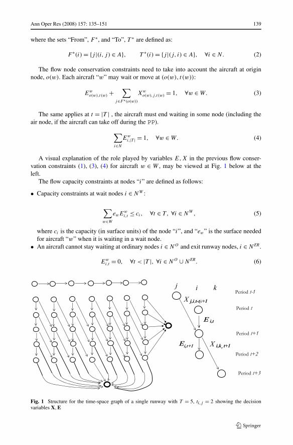
The time used by any aircraft to move along each link (i, j) ∈ A is assumed constant inthe model and it is rounded to an integer number ti,j of time subperiods. The TP-S variablesare associated to the space-temporal nodes N∗ = {(i, t),∀i ∈ N,∀t ∈ T } and space temporallinks A∗ = {(i, t), (j, t ′),∀(i, j) ∈ A,∀t ∈ T , t ′ = min{t + ti,j , |T |}}}. In Fig. 1, the righthand side provides a visual help using a simple case of a time expanded network (N∗,A∗).

The TP-S model determines the routes on the airport’s ground for a set W of aircraftduring the PP. For each aircraft w ∈ W , we define an origin node, o(w) ∈ N , a destinationnode, d(w) ∈ N , and a starting time for its route, t (w) ∈ T . In the space time network theorigin is a single node, but the destination on the space-time network consists of a set ofspace-temporal nodes defined by the nodes (i, t) ∈ N∗ with d(w) = i for the different timesubperiods if the aircraft arrives at its destination during the PP or a sink node at the end ofthe PP. The reader is directed again at the left side of Fig. 1.

The binary variables used to define the TP problem are the following ones:

Ewi,t = 1, if aircraft “w” waits in node “i” at period “t”; and 0, otherwise.

Xwi,j,t = 1, if aircraft “w” is routed from node “i” to node “j” at period “t”; and

0, otherwise.

The flows on the space time network are disaggregated for each aircraft w ∈ W andare made up with the previous binary variables Ew

i,t , Xwi,j,t . Thus the TP-S model has a

multicommodity flow structure. The feasible set of the TP-S problem is defined by themulticommodity flow conservation constraints, the flow capacity constraints, and other sideconstraints.

The flow conservation constraints at every node are:

Ewi,t +

∑

j∈T ∗(i)

Xwj,i,t+1−ti,j

= Ewi,t+1 +

∑

j∈F ∗(i)

Xwi,j,t+1, ∀t ∈ T , ∀w ∈ W, ∀i ∈ N, (1)

Ann Oper Res (2008) 157: 135–151 139

where the sets “From”, F ∗, and “To”, T ∗ are defined as:

F ∗(i) = {j |(i, j) ∈ A}, T ∗(i) = {j |(j, i) ∈ A}, ∀i ∈ N. (2)

The flow node conservation constraints need to take into account the aircraft at originnode, o(w). Each aircraft “w” may wait or move at (o(w), t (w)):

Ewo(w),t (w) +

∑

j∈F ∗(o(w))

Xwo(w),j,t (w) = 1, ∀w ∈ W. (3)

The same applies at t = |T | , the aircraft must end waiting in some node (including theair node, if the aircraft can take off during the PP).

∑

i∈N

Ewi,|T | = 1, ∀w ∈ W. (4)

A visual explanation of the role played by variables E,X in the previous flow conser-vation constraints (1), (3), (4) for aircraft w ∈ W , may be viewed at Fig. 1 below at theleft.

The flow capacity constraints at nodes “i” are defined as follows:

• Capacity constraints at wait nodes i ∈ NW :

∑

w∈W

ewEwi,t ≤ ci, ∀t ∈ T , ∀i ∈ NW, (5)

where ci is the capacity (in surface units) of the node “i”, and “ew” is the surface neededfor aircraft “w” when it is waiting in a wait node.

• An aircraft cannot stay waiting at ordinary nodes i ∈ NO and exit runway nodes, i ∈ NER.

Ewi,t = 0, ∀t < |T |, ∀i ∈ NO ∪ NER. (6)

Fig. 1 Structure for the time-space graph of a single runway with T = 5, ti,j = 2 showing the decisionvariables X,E

140 Ann Oper Res (2008) 157: 135–151

• At access to runway nodes i ∈ NAR and artificial nodes i ∈ NF only one aircraft is allowedat a time:

∑

w∈W

Ewi,t ≤ 1, ∀t ∈ T , ∀i ∈ NAR ∪ NF . (7)

• Other constraints are also related to node capacities, as it is the case for some nodes,where the total number of aircraft arriving at them during each time subperiod is limitedto only one if they are not occupied or zero if they are already occupied.

∑

w∈W

Ewi,t +

∑

w∈W

∑

j∈T ∗(i)

Xwj,i,t+1−tj,i

− 1 ≤ 0, ∀t ∈ T , ∀i ∈ NO ∪ NAR ∪ NF . (8)

TP-Sminimizes total routing time for all the flights, so the objective function τ is definedas a total weighted time expressed in number of time subperiods and spent to route allaircraft:

τ(X,E) =∑

w∈W

∑

t≥t (w)

λw

( ∑

i,j∈Ati,jX

wi,j,t +

∑

i∈NW

Ewi,t

)+

∑

i∈N

∑

w∈W

rwi Ew

i,|T |, (9)

where λw is the priority for aircraft “w ∈ W ”. rwi is the estimated time outside the PP

measured in number of time subperiods and that is necessary for aircraft “w” to arrive at itsdestination from the node “i” in the PP. rw

i is obtained using a shortest path algorithm.

3 TP-S reduced formulation

A reduced TP-S formulation may be obtained with the flow vectors Uw = (Uwa ,∀a ∈ A∗),

w ∈ W , where for all a ∈ A∗: Uwa = (Xw

i,j,t ,∀i, j ∈ A,∀t ∈ T ;Ei,t ,∀i ∈ N,∀t ∈ T ).The previous node flow conservation constraints (1) to (4) can be expressed in compact

form by means of proper node-link incidence matrices Bw and origin-destination vector bw

of each aircraft w ∈ W , with components 1, −1 or 0 depending on the associated node beingthe aircraft origin, destination or other respectively.

BwUw = bw, w ∈ W. (10)

The capacity constraints (5) to (8) that model the capacity limitations can be expressedas generic link capacity constraint such as,

∑

w∈W

ma,w1 Uw

a ≤ qa, a ∈ A∗1 (11)

or in compact form Ma1 Ua ≤ qa,∀a ∈ A∗

1, where Ua = (Uwa ,∀w ∈ W), Ma

1 is the vector ofcoefficients m

a,w1 , and A∗

1 is the set of links associated to nodes with capacity. A∗1 is defined

by A∗1 = {((i, t), (i, t + 1)) ∈ A∗ : i ∈ NW,1 ≤ t ≤ |T | − 1}.

The capacity constraint (8) that model the node access conflicts can be also expressed asgeneric node capacity constraints such as,

∑

w∈W

mi,w2 Uw

a ≤ qi, i ∈ N1 (12)

Ann Oper Res (2008) 157: 135–151 141

or in compact form Mi2Ui ≤ qi,∀i ∈ N1, where Ma

2 is the vector of coefficients mi,w2 , and

N1 = NO ∪ NAR ∪ NF .Then, TP-S can be expressed as a binary multicommodity network flow problem with

capacity constraints,

MinU τ(U)

s.t.: BwUw = bw, w ∈ W,

Ma1 Ua ≤ qa, a ∈ A∗

1,

Mi2Ui ≤ qi, i ∈ N1,

U binary.

(13)

4 Network design based on TP model

The previous TP-S is concerned with the routing problem of aircraft on the ground for afixed topology of the airport dependencies. In this section we introduce several additionalconstraints and objectives as well as decision variables into the Taxi Planning model in orderto take into account the possibility of considering certain types of short-to-medium term op-erational decisions such as temporarily closing or opening or reversing a runway, a terminal,etc. We will formulate this model in the form of a network design problem where the objec-tive function will be a weighted sum of conflicting objectives. As a distinctive characteristic,the model takes into account in the design decisions the factor of interventions of the con-trollers that monitor the evolution of the aircraft. In this sense, the model makes decisionson topology and/or aircraft routes on the ground that do not force to increase the number ofinterventions thus trying to minimize situations that would require a mandatory preventiveaction. The resulting model shall be referred to as a Taxi Planning Network Design for ShortTerm operations or TPND in short.

4.1 Incorporating short-to-medium term operational decisions into the model

In practice, the following (conflicting) objectives are to be minimized under low to mediumcongestion situations during the PP, from higher to lower priority:

1. Number of interventions of controllers in order to solve possible conflicts.2. Total delay of outgoing traffic.3. Total time until take-off or arrival at a final parking.4. Total delay of incoming traffic.

In situations of high congestion an objective that takes priority is the total number ofarrivals at the final destination on the ground (parking or terminal) plus the total number oftaking-offs. We will now present the formulation of the objectives mentioned above.

4.1.1 Number of controller interventions

The design decisions given by the TPND model must take into account the practical feasibil-ity of their solutions. Airport Management Authorities usually consider that one of the mostimportant operational tasks of the controllers is their surveillance and capacity to preventany kind of conflicts. For normal operational conditions, design solutions regarding aspectsof the airport topology must be considered so that one of the aspects that enforce the secu-rity of the operations is to make the task of the airport controllers as easy as possible. Inthis model a conflict arises when two or more aircraft approach at a point and at least one

142 Ann Oper Res (2008) 157: 135–151

of them is going to cross it and the crossing trajectories either coincide or are separated bya short time. Remember that constraints (8) ensure that two trajectories do not coincide intime at a single node of the network model. This will cause the intervention of a controllerin order to ensure that some aircraft stop, thus guaranteeing that the conflict point is crossedsafely by only one of them at a time. A set of constraints modelling the proximity in timeof two trajectories at a conflict point and an objective function that provides the number oftimes during the PP that controllers enter into action will be developed in this section.

Clearly, (8) prevents more than one aircraft from accessing node i at a time. Conse-quently, trajectories cross each other separated by a time subperiod of �t seconds. Also, asthe right hand side of (8) can be considered the excess of aircraft at node i during time sub-period t ∈ T , (8) imposes that no excess of aircraft may exist at node i otherwise, solutionsprovided by the model would permit crashing of two trajectories. The concept of excessaircraft at a node i and during time t ∈ T can be extended to a set of nodes of the airportnetwork model for ν + 1 time subperiods. The set of nodes where a zero excess would bedesirable due to safety of operations will be referred to as a conflicting point and, on thesepoints, in case of positive excess aircraft, the intervention of controllers would be required.In other words, at conflicting points only one aircraft is allowed each ν time subperiods oralso, trajectories might be separated ν subperiods in time whenever possible.

Let K be the set of conflicting points on the airport. Let KA(K) and KN(K) be the set ofincoming arcs to the conflicting point K ∈ K and the set of nodes inside the conflict pointK ∈ K respectively, where there can be aircraft waiting.

Let xi,j,t = ∑w∈W Xw

i,j,t be the total number of aircraft traversing link (i, j) at time t ∈ T

and let ei,t = ∑w∈W Ew

i,t be the total number of aircraft staying at node i ∈ N during timesubinterval t ∈ T . At a conflicting point K ∈ K and as a generalization of (8), the excessaircraft at time t ∈ T for a preventive horizon of ν time subperiods is denoted by CK,t andis given by:

CK,t =t∑

�=max{t−ν,2}

( ∑

(i,j)∈KA(K)

�−ti,j ≥1

xi,j,�−ti,j +∑

i∈KN (K)

ei,�−1

)− 1,

K ∈ K, 2 ≤ t ≤ |T |. (14)

Note that the excess aircraft expressed in (14) is defined only for t ≥ 2 because it isimplicitly assumed that the PP starts without excess at K ∈ K, or equivalently that the initialdistribution of aircraft on the airport is such that

∑i∈KN (K) ei,1 ≤ 1 at K ∈ K.

Under the previous definition in (14) of CK,t , the intervention of a controller will occurat time t ∈ T for K ∈ K if CK,t > 0. Then a convenient objective can be the minimizationof the total number of interventions. For this purpose the binary variables γK,t need to bedefined:

CK,t > 0 ⇒ γK,t = 1,(15)

CK,t ≤ 0 ⇒ γK,t = 0.

Logical conditions (15) can be readily expressed as linear constraints and the followingsharp bound for CK,t can be useful. It must be noticed that, due to (8) no more than oneaircraft can be present on a link at a time and also no more than one aircraft can be stayingat a node at a time. Because the excess aircraft CK,t is computed for ν previous additionaltime subperiods, then CK,t must be bounded by:

CK,t ≤ ν · (|KA(K)| + |KN(K)|). (16)

Ann Oper Res (2008) 157: 135–151 143

Using the previous bound (16) on CK,t , the following linear constraints at a conflictingpoint K ∈ K and time 2 ≤ t ≤ |T |,

CK,t ≤ ν · (|KA(K)| + |KN(K)|) · γK,t , γK,t ∈ {0,1}, (17)

are equivalent to the following logical relationships between CK,t and γK,t :

CK,t > 0 ⇒ γK,t = 1,(18)

CK,t ≤ 0 ⇒ γK,t ∈ {0,1}(i.e. no additional constraints on γK,t )

Then, if the total number of controller interventions IC on all the conflicting points duringthe PP is expressed as:

IC =∑

K∈K

∑

2≤t≤|T |γK,t (19)

and this objective is to be minimized, then, if for some K ∈ K, 2 ≤ t ≤ |T | it happens thatCK,t ≤ 0 this implies that γK,t = 0. Consequently, linear constraints (17) together with theminimization of a linear objective that includes IC as a positive term is equivalent to thelogical conditions (15).

4.1.2 Worst routing times and delays

Let the routing time τw for aircraft w ∈ W be defined in terms of the flow vectors Uw as:

τw(Uw) =|T |−1∑

t=1

( ∑

(i,j)∈A

ti,jXwi,j,t +

∑

i∈NW

Ewi,t

)+

∑

i∈NW

rwi Ew

i,|T |. (20)

If λw is a coefficient for the priority of aircraft w ∈ W , then the weighted total routingtime τ can be expressed as in (9).

In addition to the weighted routing times τ given by (9) it is convenient to take intoaccount the worst routing time τ given by:

τ = Maxw∈W {τw}. (21)

The worst travel time can be included by means of the following constraints,

τw(Uw) ≤ τ , w ∈ W (22)

with τw defined in terms of the flow variables Xwi,j,t and Ew

i,t by (20).Delays Dw

IN, DwOUT of incoming and outgoing traffic are given by:

DwIN =

∑

t∈T

∑

i∈NW

Ewi,t , ∀w ∈ WA. (23)

where WA is the set of aircraft arriving at the airport during the PP.

DwOUT =

∑

t∈T

∑

i∈NW

Ewi,t , ∀w ∈ WD, (24)

where WD is the set of departing aircraft during the PP.

144 Ann Oper Res (2008) 157: 135–151

Clearly, the worst routing times for aircraft either τ or the related delay DwIN,D

wOUT may

be objectives that conflict with IC , the number of controller interventions defined in theprevious subsection in case of congestion, because reducing the number of times that space-time trajectories of two or more aircraft are close to each other generally must result indelays for waiting or adopting routes with greater travel times.

4.1.3 Number of arrivals and take-offs

A magnitude that can be also monitored after solving the TNDP-S model is the totalthroughput T = T − + T + comprised of the total number of take-offs, T −, and arrivalsat destinations on ground, T +, within the PP.

The number of arrivals on the ground is:

T + =∑

t∈T

∑

w∈WA

∑

i∈NER

∑

j∈F ∗(i)

Xwi,j,t . (25)

The number of take-offs during the PP is:

T − =∑

t∈T

∑

w∈WD

∑

i∈NAR

∑

j∈F ∗(i)

Xwi,j,t . (26)

As with the aircraft travel times of previous subsection, the total airport throughput Tmay be in conflict with IC as the effect in minimizing IC may lead to a reduction in theairport’s capacity.

4.2 Design decision variables

Design variables are related to elements of the TP-S network. Let y be a vector of binaryvariables that will be associated to open/close during the whole PP links within a reducedsubset A of links with capacity A∗

1. If yi,j is the decision variable associated to link (i, j) ∈ A

with capacity qi,j , then, clearly the constraints linking the flow variables in U to the decisionvariables will be:

∑

t∈T

∑

w∈W

Xwi,j,t ≤ qi,j yi,j , ∀(i, j) ∈ A (27)

or in compact form HaUa ≤ qaya , ∀a ∈ A.

The design variables may belong to a design feasible set Y , that could be defined bymeans of budget or environmental constraints.

4.3 TPND formulation

Let g(y) be the link location costs associated with the decisions yij . It will be assumedthat it is a linear function g(y) = ∑

(i,j)∈A ci,j yi,j with nonnegative coefficients ci,j . TheTPND model can be stated in the form of a binary optimization problem that minimizesa multiobjective function of the decision variables U ∈ {0,1}, y ∈ Y during the PP whileensuring that the airport constraints can be satisfied. Along with them, constraints (17) thatmodel controllers intervention and the ones that model the worst travel time (22) must alsobe taken into account. This set of constraints will be expressed simply as �1U ≤ �2γ , where

Ann Oper Res (2008) 157: 135–151 145

γ = (· · ·γK,t · · · ; t ∈ T ,K ∈ K), are defined in (15). Adding the constraints between flowvariables and decision variables, the TPND problem can be stated as:

MinU,y,γ,τ φ

s.t.: BwUw = bw, ∀w ∈ W,

Ma1 Ua ≤ qa, a ∈ A∗

1,

Mi2Ui ≤ qi, i ∈ N1,

τw(Uw) ≤ τ , ∀w ∈ W,

HaUa ≤ qaya, ∀a ∈ A,

�1U ≤ �2γ,

U, γ binary, y ∈ Y,

(28)

where φ is a weighted sum of objectives given by (9), (19), (23), (24), (25), and (26), takinginto account the worst travel time τ and the cost g associated to the binary variables y:

φ = ατ τ + αLg(y) + αICIc + αOUT∑

w∈WD

DwOUT + αIN

∑

w∈WA

DwIN + ατ τ + αT T , (29)

where ατ ,αL,αIC, αOUT, αIN, ατ , αT ≥ 0 and ατ + αL + αIC + αOUT + αIN + ατ + αT = 1.The new TPND defined with this objective function is a multiobjective problem and dif-

ferent methodologies would be applied. A simple but effective technique is shown in thenext section in order to manage the computational difficulties that may arise in balancingthe components of the objective function regarding especially the inclusion of the termsrelated to the number of controller interventions.

5 Running the TPND

The test airports are those depicted in Figs. 2 and 3 which shall be referred to as airport J1and J2 respectively. For each airport a PP of 30 minutes has been considered using timesubintervals of 30 seconds.

Airport J1 is comprised of two separate runways one of them for take off and the otherone for landing. Airport J2 has a single runway for taking off/landing purposes. The use fortaking-off or landing is conditioned by meteorological conditions and not for the demandduring the PP and is therefore outside of decisions that can be considered by the TPNDmodel. Airport J2 can be considered as an extension of J1 with additional corridors foraccess/exit to/from the taking-off/landing runways and with a more complex mix runway.Both airports have three parking platforms, each parking platform consisting of three park-ing locations with capacity for five aircraft. In the computational tests all the aircraft beingconsidered have equal characteristics, requiring an extension of nearly 1700 m2 for parkingpurposes. In the diagrams shown in Figs. 2 and 3 links joining two nodes model corridorsections which can be bidirectional accordingly to the double/single arrow for the link andhave equal length (309 m), excluding those with a black circle in between which are ofdouble length. It is allowed that an aircraft stays waiting on these double length links. Thisis captured in the graph model splitting the double length links with an intermediate nodefor modelling the possibility of a wait. Aircraft are supposed to move at a constant speedof almost 40 km/h through the corridors and thus movements through a corridor section aredone in one subperiod (i.e., ti,j = 1). Waits can occur at any of the nodes in the diagramsfor airports J1 and J2, excluding those that are exit from landing runways (NER nodes) ornodes that are runway headers (NAR nodes).

146 Ann Oper Res (2008) 157: 135–151

Fig. 2 Test airport J1

Fig. 3 Test airport J2

For airport J1, the points where it is possible that interventions of controllers may occurare NAR, O1, O2, O3, NW2, NW3 and NW4, whereas in airport J2 the points are O5, O6, O1,O2, NW3, O7, NW4, NW5 and NW6. A period ν of three time subintervals has been consideredfor the time that may trigger an intervention of a controller.

Ann Oper Res (2008) 157: 135–151 147

Table 1 Problem size

vars. N.C. I.C. E.C.

J1 6057 2155 5362 2167

J2 15674 6089 10346 5981

vars = N. of variables

N.C. = Network constraints

I.C., E.C. = (In)equality constraints

For airport J1 the decision being considered is the capacity at node NW1 in terms of thenumber of aircraft that can stay waiting. For airport J2 the decisions taken into account bythe TPND model are:

1. The capacities at nodes NW1, NW2, NW3 also expressed in number of aircraft that can staywaiting at each of these nodes. The range of possible capacities is set from 0 to an upperbound of 5 aircraft for NW1, NW2 and a range of 1 to 5 for NW3. Simultaneously to theprevious decisions, the possibility of opening/closing exit from runways NER1, NER2,NER3 is also considered.

2. As before, capacities within an equal set of ranges for waiting nodes NW1, NW2, NW3 andsimultaneously, for the exit from runways NER1, NER2, NER3 the possibility of beingopened only two out of three at most.

The coefficients adopted for the linear function g(y) that models the decision costs as-sociated to decisions y were set to one in all cases. In all the computational tests the resultsshowed that, for airport J1 a capacity of one aircraft suffices at node NW1 and also at nodesNW1, NW2, NW3 in airport J2. With regard to exit from runways NER1, NER2, NER3 forairport J2 all three exits should be opened if possible and in case of choosing a maximumof two of them, exits NER2 and NER3 are preferable.

The tests of the model have been performed on a Pentium IV, 1.7 GHz with 256 MB ofmemory using the AMPL-CPLEX System. The size of the problems solved for the tests isgiven in Table 1.

The layout of Tables 2, 3 and 4 is as follows. Each table is comprised of a set of runsand for each subset of runs the set of weighting parameters in the objective function is givenin the initial record. The total number of aircraft operating on the airport is expressed incolumn |W |, whereas the number of aircraft that complete their operation within the PP isin column T . The number of aircraft arrival aircraft is given in column |WA|, whereas thenumber of departing aircraft is given in column |WD|. From these, aircraft that arrive at itsparking destination within the PP is given by T+ and the total number of aircraft that take-off within the PP is given in T−. IC is the total number of controller’s interventions, DIN

and DOUT are the total delay time for aircraft entering/leaving the airport respectively, τ isthe worst travel time amongst all the aircraft operating on the airport, τ is the total weightedtime. Finally column B&B is the number of nodes of the tree expanded during the executionof the Branch and Bound algorithm in the run.

The first set of tests have were performed on Airport J1 in order to show the difficultyof dealing with the modeling of the number of interventions of the Airport controller’s,i.e. constraints (17). A total of 14 runs have been performed for airport J1. Runs 1 to 6were done with αIC = 0.5 with an increasing number of aircraft entering/leaving J1. Thecomputer requirements (column TCPU in seconds) increase drastically as |W | increases anda run with |W | = 8 was abandoned. Runs 7 and 8 have adopted as objective function just the

148 Ann Oper Res (2008) 157: 135–151

Table 2 Tests on airport J1

αIC = 0.5, ατ = 0.2, αIN = 0.15, αOUT = 0.1, αL = 0.0499, αT = 0, ατ = 0.0001

φ TCPU |W | T |WA| T+ |WD | T− IC DIN DOUT τ τ B&B

1 3.09 0.06 1 1 0 0 1 1 0 0 0 4 4 0

2 4.84 0.21 2 2 1 1 1 1 0 1 0 8 12 0

3 5.84 0.28 3 3 1 1 2 2 0 1 0 8 17 0

4 8.84 6.57 4 4 2 2 2 2 1 3 0 11 28 0

5 11.89 38.73 5 5 2 2 3 3 1 6 0 14 41 1

6 17.39 303.6 6 6 3 3 3 3 8 6 0 15 51 2

αIC = 0, ατ = 1.0, αIN = αOUT = αL = αT = ατ = 0

7 29.0 0.46 6 6 3 3 3 3 187 2 0 7 29 0

8 105.0 59.26 16 16 7 7 9 9 187 3 0 14 105 0

αIC = 0, ατ = 0.9, αIN = αOUT = 0, αL = 0.1, αT = ατ = 0

9 99.10 83.39 16 16 7 7 9 9 187 3 0 14 105 0

10 30.70 0.57 6 6 3 3 3 3 187 0 0 7 29 0

αIC = 0.001, ατ = 0.899, αIN = αOUT = 0, αL = 0.1, αT = ατ = 0

11 99.06 191.6 16 16 7 7 9 9 71 3 0 12 105 620


12 98.74 265.1 16 16 7 7 9 9 69 3 0 9 105 1496


13 97.30 110.2 16 16 7 7 9 9 69 3 0 9 105 338


14 95.50 147.0 16 16 7 7 9 9 69 3 0 9 105 508

total weighted time τ and thus the constraints on the number of controller interventions areinactive. Clearly, run number 8 with 16 aircraft is solved very swiftly without the need ofexpanding a Branch and Bound tree (i.e. the initial linear relaxation of the problem providesthe solution). In this case column IC is meaningless as αIC = 0. These runs are includedin order to show how the constraints on the number of controller interventions affect thecomputation times. Runs 9 and 10 show that the inclusion of the component with decisioncosts can be handled also very well. Runs 11 to 14 show that in order to take into accountin the solutions the IC factor, different runs with increasing values for αIC should be doneuntil no enhancement is observed for IC(= 69).

For airport J2 the same procedure followed in the previous example is applied. Runs1 to 5 in Table 3 have been made with |W | = 11 aircraft. Starting from the objective withcoefficients ατ = 0.9 and αL = 0.1, the presence of the factor IC is increased obtainingsolutions with bigger IC . This time the total weighted time τ does not degrade as the factorIC can not be lowered from 46. Notice that the computer requirements are also increasing

Ann Oper Res (2008) 157: 135–151 149

Table 3 Tests on airport J2

αIC = 0, ατ = 0.9, αIN = αOUT = 0, αL = 0.1, αT = ατ = 0


1 78.60 8.59 11 11 4 4 7 7 235 3 0 13 82 0


2 78.24 19.28 11 11 4 4 7 7 46 6 0 13 82 87


3 76.80 40.65 11 11 4 4 7 7 46 3 0 12 82 269


4 75.00 72.34 11 11 4 4 7 7 46 3 0 12 82 509


5 71.39 377.71 11 11 4 4 7 7 46 6 0 12 82 3637

6 99.8 1943.5 16 16 7 7 9 9 69 6 0 12 116 11059a


7 108.7 56.31 16 16 7 7 9 9 68 7 0 12 116 264


8 106.8 82.48 16 16 7 7 9 9 68 7 0 13 116 340

aExecution interrupted

Table 4 Tests on airport J2; Select two out of three exits from runway



1 108.7 65.17 16 16 7 7 9 9 69 7 0 11 116 541


2 106.8 104.28 16 16 7 7 9 9 69 5 0 12 116 769


3 104.5 142.15 16 16 7 7 9 9 69 6 0 12 116 555


4 102.1 1468.1 16 16 7 7 9 9 69 7 0 12 116 10523

150 Ann Oper Res (2008) 157: 135–151

as αIC increases. Runs 6 to 8 correspond to a demand with |W | = 16 aircraft and the sameeffect on the CPU time is observed. Run numbers 7 and 8 is for αIC = 0.01 and αIC = 0.05and also |W | = 16. It must be noticed that this time trying to optimize IC has some effecton the travel times as shown by the worst travel time τ . Run number 6 for αIC = 0.2 had tobe interrupted after more than half an hour running, probably at a solution very close to theoptimum because it is obtained a solution very similar to the ones obtained in runs 7 and 8.

Table 4 shows the results obtained by the TNDP-S model with airport J2 with the ad-ditional constraint of choosing two out of the three exits from the landing runway. Runs 1to 4 are for increasing values of αIC = 0.01,0.05,0.1,0.15. As before, increasing values ofTCPU with small impact on the travel times of aircraft can be observed.

6 Conclusions and extensions

In this paper a network design model for the ground airport’s Taxi Planning operations(TPND for short) has been presented. The TPND model has been formulated as a binarymulticommodity network flow problem with side constraints developed on a time-spacenetwork under the same approach on which the short term Taxi Planning model in Marín(2006) was developed. The model adopts a multiobjective approach by balancing severalobjectives that are the most relevant aspects usually taken into account in real practice bythe Spanish airport management authorities: total weighting and routing time on the ground,input and output airport’s throughput, worst routing time and number of interventions ofcontrollers at a preselected set of conflicting points. The TPND model has been shown tobe an adequate tool to analyze the optimal airport configuration considering aircraft conges-tion and airport facilities, when at the design level there are decisions closely related to thedynamic aspects of the routing of aircraft on the ground.

The computational experiments have been run using Branch and Bound, and they havebeen carried out with two simplified airport networks, taken from actual data of Madrid-Barajas Airport, supplied by Aeropuertos Españoles y Navegación Aérea, the Spanish air-port management corporation in order to better illustrate the key aspects of the model. Com-putational tests on these networks have been run using different weights of the objectivefunction in order to show the most relevant aspects of the implicit multicriteria decisionprocess on which the model relies as well as to show the sources of computational difficultythat may arise in solving the optimization problems. It has been shown how the inclusionof factors relative to the number of interventions of the controllers is the source of the ma-jor computational difficulties in the model and also how these difficulties can be avoidedanalyzing the model using different runs.

As extensions of the current work a complete multiobjective analysis may be performedand the good computational results shown on the test networks permit to consider furtherextensions of this design model. In the algorithmic field it is appealing and necessary todevelop of more efficient computational methods in order to solve larger problems. In thissense the multicommodity network flow structure suggests the dualization of the side con-straints making the Lagrangean relaxation a clear candidate.

References

Anagnostakis, I., Clarke, J.-P., Böhme, D., & Völckers, U. (2001). Runway operations planning and control:sequences and scheduling. Journal of Aircraft, 38(6), 988–996.

Ann Oper Res (2008) 157: 135–151 151

Andersson, K., Carr, F., Feron, E., & Hall, W. D. (2002). Analysis and modeling of ground operations at hubairports. 3nd USA/Europe Air Traffic Management R & D Seminar, Napoli, 13–167 June 2002.

Gotteland, J. B., Durán, N., Alliot, J. M., & Page, E. (2000). Aircraft ground traffic optimisation. Paper ofEcole Nationale de l’Aviation Civile.

Idris, H. R., Delcaire, B., Anagnostakis, I., Feron, E. Clarke, J.-P. & Odoni, A.R. (1998). Identification offlow constraint and control points in departure operations at airport systems. Paper AIAA-98.4291American Institute of Aeronautics and Astronautics.

Idris, H., Clarke, J.-P., Bhuva, R., & Kang, L. (2002). Queueing model for taxi-out time estimation. Air TrafficControl Quarterly, 10(1), 1–22.

Marín, A. (2006). Airport management: taxi planning. Annals of Operation Research, 143, 189–200.Pujet, N., Delcaire, B., & Feron, E. (1999). Input-output modeling and control of the departure process of

busy airports. Report No. ICAT-99-3. MIT International Center for Air Transportation.Stoica Dragos, C.M. (2004). Analyse, represéntation et optimisation de la circulation des avions sur une

plate-forme aéroportuaire. Thesis Laboratoire d’Analyse et d’Architecture des Systèmes du CNRS,Toulouse, France.

Documents

Network design: taxi planning - … · Network design: taxi planning Angel ... as a basis for any airport network design or maintenance model. ... a detailed methodological proposal