Network Effects and Personal Influences: The Diffusion of an Online

Network Effects and Personal Influences: TheDiffusion of an Online Social Network

Zsolt Katona, Peter Pal Zubcsek and Miklos Sarvary∗

August 7, 2010

∗Zsolt Katona is Assistant Professor of Marketing at the Haas School of Business, UC Berkeley, Berke-ley, CA 94720. Peter Pal Zubcsek is Assistant Professor of Marketing at University of Florida, Gainesville,FL 32611. Miklos Sarvary is Professor of Marketing at INSEAD, Bd. de Constance, 77305, Fontainebleau,France. E-mail: [email protected], [email protected], [email protected]. Peter PalZubcsek’s work was supported by the Sasakawa Young Leaders Fellowship Fund.

1

Network Effects and Personal Influences: The Diffusion of anOnline Social Network

Abstract

We study the diffusion process in an online social network given the individual connections

between members. We model the adoption decision of individuals as a binary choice affected by

three factors: (1) the local network structure formed by already adopted neighbors, (2) the

average characteristics of adopted neighbors (influencers), and (3) the characteristics of the

potential adopters. Focusing on the first factor, we find two marked effects. First, an individual

who is connected to many adopters has a higher adoption probability (degree effect). Second, the

density of connections in a group of already adopted consumers has a strong positive effect on the

adoption of individuals connected to this group (clustering effect). We also record significant

effects for influencer and adopter characteristics. Specifically, for adopters, we find that their

position in the entire network and some demographic variables are good predictors of adoption.

Similarly, in the case of already adopted individuals, average demographics and global network

position can predict their influential power on their neighbors. An interesting counter-intuitive

finding is that the average influential power of individuals decreases with the total number of their

contacts. These results have practical implications for viral marketing in a context where,

increasingly, a variety of technology platforms are considering to leverage their consumers’

revealed connection patterns. In particular, our model performs well in predicting the next set of

adopters.

Keywords: Diffusion, Social Networks, Network Marketing.

2

1 Introduction

While the importance of word of mouth (WOM) in influencing consumer decisions has long been

recognized by marketers, it has been difficult to measure its impact and to efficiently use it for

commercial purposes until recently. Modern technology, however, has gradually transformed

social interactions among people. On average, we communicate more using some sort of

technology platform (phone, VoIP, e-mail or chat) and our frequent contacts are readily available

to the owner of these communication platforms. With the emergence of Web 2.0 technologies,

media such as blogs, instant messaging (e.g. msn.com) and social networking web-sites (e.g.

Facebook.com) are becoming ubiquitous and they all provide a “map” of communication paths

among their users. Social networking sites, such as MySpace or Facebook, are particularly

interesting examples. They represent rich and popular communication interfaces for hundreds of

millions of users. On these sites, users exhibit their demographics as well as their preferences by

carefully editing (decorating) their profiles. More importantly, they explicitly link to their friends,

in this way, revealing their likely communication patterns. In the last five years, social networks

have populated the world, often attracting a critical proportion of a country’s population.

Cyworld, for example, claims to count over 40% of Koreans among its membership base, whereas

Facebook has over 400 million members worldwide and has recently surpassed Google in

becoming the most visited website in the US.

The increased importance of technology platforms for social interactions has raised the

interest of product marketers who seek to explore these as new advertising/promotion media.

Indeed, social networks’ revenue models are primarily based on advertising, although, so far, the

use of (mostly) banner-type advertising has produced disappointing results.1 Increasingly,

marketers believe that the efficient way of using social networks for marketing relies on

harnessing WOM, by analyzing the network of members’ connections. For example, Google has

recently filed a patent for an algorithm that identifies so-called “influencers” on social networks.

Several other firms (e.g. Idiro and Xtract) provide network analysis for the telecom sector as well

as for various Web 2.0 platforms in order to assist in viral marketing campaigns. Indeed, social

1See, for example, “Social graph-iti”, in The Economist, 20. October, 2007, pp.77, or “Google: Harnessing thePower of Cliques”, in Business Week, 6. October, 2008, pp.50.

3

networks represent but one area where network analysis might be used for WOM marketing.

Other technologies (blogs, telecom, virtual worlds, etc.) that record consumers’ communication

patterns are also adapted to such techniques. In all these cases, the basic idea is that

understanding the network structure of individual consumers can help implement effective viral

marketing strategies.

The assumption underlying all these “network marketing” techniques is that network

information can help identify influencers and predict consumers’ adoption probabilities. The goal

of this paper is to verify this assumption and to identify how the network structure drives

adoption. Specifically, we develop and empirically test an individual level diffusion model that

explicitly takes into account the micro-structure of interpersonal connections between potential

adopters. Our empirical application studies the growth of a country-specific social network site,

where membership can only be acquired by receiving an invitation from an existing member. In

this context, we study the adoption process of network memberships at an early stage of the site’s

development. We assume that, gradually, the social network site replicates people’s real-life

social connection patterns. Thus, recording the site’s membership network at a much later point in

time, we can assume that it reflects people’s real-life social networks quite accurately. Then,

looking back in time, we observe a diffusion process of membership on this “ultimate” or “final”

network.2

Our primary research objective is to uncover the effects that differences in individuals’

connection patterns have on the diffusion process. Motivated by conceptual as well as practical

considerations, we distinguish three factors that may affect a potential adopter’s adoption

decision. The first factor, that we call “network effects”, relates to the influence of the structure of

connection patterns of the potential adopter’s already adopted neighbors. The second factor, that

we call “influencer effects”, refers to the (average) individual characteristics of already adopted

network members on their not-yet-adopted neighbors. As opposed to the previous factor that

concentrates on the impact of the structure, under influencer effects, we essentially measure the

(average) influential power of every adopter. The average characteristics describing influencers

2It is important to realize that the present paper does not study a network growth or network formation processbut, rather, a diffusion process on an already existing network of potential adopters. Of course, the results depend onthe validity of the assumption that we have indeed captured the relevant social network by observing the membershipnetwork at a late stage. In our empirical application, we test this assumption in various ways (see Section 4.4.3).

4

may be demographics, such as age for example, but they may also include measures that describe

the global network position of the influencers, i.e. their position in the “final” social network

observed. Finally, the third factor, called “adopter effects” captures the effects of the adopter’s

individual characteristics. As for influencers, these characteristics include both demographics as

well as characteristics describing the adopter’s global network position. Depending on data

availability and legislative constraints, marketers can use each of these categories of variables to

identify potential marketing targets in order to influence the adoption process. They can target

members of the network who have already adopted the promoted product or potential adopters

who have yet to adopt. In both cases, potential marketing targets can be selected based on their

individual characteristics or, alternatively, based on the local network structure surrounding them.

Our model helps identify potential adopters by predicting the next set of adopters substantially

better than models based solely on demographic variables.

In our choice of network variables, we rely on diffusion theory, as well as previous

research in sociology. In particular, individuals who are related to many already adopted members

may have higher adoption probability since their related partners can provide more information

about the service or innovation in question, ultimately exercising greater joint influential power.

We call this the degree effect, after the number of connections (degree) an individual has. In

addition to the number of connections, the density of connections in a group of already adopted

users may also affect the adoption of individuals being linked to the members of this group. A

more tightly connected group should have a stronger influence on its members. We call this effect

the clustering effect. We find strong empirical evidence supporting the presence of both the

degree effect and the clustering effect, as well as a positive interaction between them.

Beyond network effects we also find strong influencer and adopter effects on the adoption

probability of potential network members. For example, some demographic characteristics (e.g.

age, gender) can predict adopters’ influential power on their neighbors. Similarly, demographic

variables can also predict potential adopters’ propensity to adopt. More interestingly, variables

that describe individuals’ position in the social network (e.g. the number of their contacts, how

connected these neighbors are or the extent to which they are interconnecting parts of the

network) are also good predictors of both influential power and adoption propensity. From both a

5

theoretical and practical perspective, a particularly interesting empirical result is that the average

influential power of individuals is lower the larger their social network is. This suggests that a

high number of friends dilutes the influential power that an individual has on each of his/her

friends. We also find some evidence for that the same influential power is higher the more the

actors occupy a “brokering” position among their contacts.

The rest of the paper is organized as follows. The next section relates our work to the

literature and highlights our points of departure. Section 3 sets up the stochastic network-based

diffusion model and introduces the network measures used. Section 4 presents the empirical

analysis, including extensive validity tests. Finally, Section 5 discusses the results, concludes and

highlights a few limitations.

2 Related Literature

Our work draws on two broad research streams: (1) the marketing literature on new product

diffusion and (2), the sociology literature on social network analysis.

The large body of quantitative research on new product diffusion is based on models that,

for the most part, ignore connection patterns between individuals. Like most of its

generalizations, the famous Bass-model (1969) implicitly assumes that every consumer is

connected to every other consumer, and estimates a uniform interpersonal influence (interpreted

as WOM) on this (assumed-to-be) complete network. This typically also applies to diffusion

models that attempt to take into account consumer heterogeneity.3 While these models allow for

heterogeneous WOM effects, they still ignore the network structure of the adopter population.

Given the central role of WOM communication for the diffusion process, there has been a clear

call in the literature to incorporate the fine-grain structure of interpersonal connections in

diffusion models (see Mahajan, Muller and Bass 1993, 1990). While various models have been

developed to address this call (e.g., Goldenberg, Libai and Muller (2001, 2002) or Shaikh,

Rangaswamy and Balakrishnan (2005), see Valente (2005) for a review), these could only be

3See e.g., Oren and Schwartz (1988) and Urban and Hauser (1993) for early papers and Goldenberg, Libai andMuller (2002) and Van den Bulte and Joshi (2007) for more recent applications.

6

tested on aggregate data.4

In recent years, various technological innovations have made it finally possible to access

network data on the interpersonal relationships between consumers. Models to assess the impact

of network characteristics on the diffusion process have finally been developed and used in

empirical studies. For example, Godes and Mayzlin (2004) studied how WOM can be a driver of

personal preferences in an environment where consumer communication via newsgroups is

observed. Van den Bulte and Lilien (2001) analyzed the Medical Innovation data set which tracks

the medical community’s understanding of a new drug. To obtain the structure of WOM, they

combined data from two overlayed relationship networks (“discussion” and “advice”) to get a

social influence weight matrix over the doctors whose behavior was recorded. They then

estimated an individual-level diffusion model to demonstrate that earlier findings on social

contagion over the same network were confounded with the marketing efforts (pricing and

promotion) of the manufacturer. Nair, Manchanda and Bhatia (2010) studied physician

prescription behavior and found that opinion-leaders in the physician’s reference group may have

a significant influence on the physician’s behavior. In another domain, Hill, Provost and Volinsky

(2006) used telecommunication data to provide evidence that those customers having

communicated with a customer of a particular service have increased likelihood of adopting that

service. Recently, Iyengar, Van den Bulte and Valente (2008) investigated the relationship

between self-reported leadership and sociometric leadership, that is, when a person is nominated

by others as someone they turn to for advice. They found that these two types of opinion

leaderships are only weakly correlated and that there are significant differences between the

adoption behavior of different types of opinion leaders. Studying a different type of network,

Stephen and Toubia (2010) examined the role of the link structure in seller networks, where links

facilitate customers’ navigation between different stores. They found that the network had a

positive overall effect on store performance and that the position of stores in the network had a

significant effect on their profitability.

4Goldenberg, Libai and Muller (2001, 2002) generated adoption data by applying stochastic cellular automatamodels to simulate the diffusion process on a two-dimensional grid. In Goldenberg et al. (2002), they compared theresults of their simulations with consumer electronics sales data to explain double-peaked diffusion curves, observedin many product categories. Shaikh, Rangaswamy and Balakrishnan (2005) developed a diffusion model taking intoaccount local network characteristics. They demonstrated how it may be used to infer structural properties of theconsumer network from aggregate sales data.

7

Our work directly follows this stream of research. Our primary goal is to understand how

network characteristics (particular patterns of connections between already adopted network

members) may influence the adoption probabilities of their not-yet-adopted peers. To establish

this relationship, we estimate a discrete-time proportional hazards model. This is the same

approach that Bell and Song (2007) follow to estimate network effects on purchase behavior

across regions in the US. However, as in our data set we can observe the individual network

connections of participants, we are able to use the same approach to study the impact of personal

network structure on adoption.

How network structure affects social influence has been extensively studied in sociology,

although only in small social networks.5 An influential paper by Krackhardt (1998) suggests that

when assessing the influence individuals’ contacts have over them, we should not only count the

number of related actors but look at how those relationships are embedded in the entire network of

relationships. Coleman (1988) and later Burt (2005) establish two important social phenomena,

which may be tied to structural properties of the network. When two related individuals are

connected to the same third parties, the network becomes better at transmitting information, and

ultimately the affected relationships become stronger. Burt (2005) labels this as network closure.

He argues that the shared third parties create redundant paths for information flow, leading to

increased trust between the two related actors. As a consequence, friends of individuals in social

networks are typically very densely connected to each other compared to the average connectivity

in the network (Watts and Strogatz 1998). This is consistent with Granovetter (1973) and Rogers

(2003), who stated that social networks in general consist of clusters of densely connected

individuals with strong ties among them, and sparse weak ties connecting such clusters to each

other. Burt (2005) highlights another phenomenon related to social networks’ structural

properties, namely the fact that individuals interconnecting these clusters may have higher

influence on their peers because they have control over information originating from other groups.

This phenomenon is termed brokerage and the argument is often cited as structural hole theory

(Burt 2005). These arguments will provide critical input for our network measures.

Our model is partly based on the approaches proposed by Holtz (2004) and Shaikh,

5See also relevant early studies in marketing: Reingen and Kernan (1986) and Reingen, Foster, Brown et al. (1984).

8

Rangaswamy and Balakrishnan (2005). However, these papers do not estimate the adoption

process at the individual level. The former paper attempts to disaggregate the Bass-model to the

network level and uses simulations to confirm the results, whereas the latter compares the fit of a

small-world-based diffusion model to the traditional models using aggregate-level data. In this

paper, on the other hand, we develop and estimate an individual-level diffusion model, where

each individual is described both by her local network characteristics and demographic

information. At any point in time during the adoption process and for each potential adopter, we

compute the network spanned by their already adopted peers. We then estimate how the structure

of the network of their adopted peers affects the adoption probability of the potential adopters.

Further, we also show empirically how network characteristics of already adopted individuals

may predict their influential power on others. The estimates also provide insights on some of the

common sociological theories in network analysis. Our model is presented next.

3 Model

We start by describing the individual level adoption model. This is followed by the description of

network measures.

3.1 The Adoption Process

To examine the process of diffusion over a social network, we use a hazard rate model. We

assume that all members of the network are potential adopters of a certain product or service. The

relationships among network members serve as paths for WOM communication, through which

network members may influence each others’ adoption. We denote such a social network by

G(V,E), where V is the set of potential adopters and E is the set of symmetric binary

relationships among members of V .

By neighbors of a potential adopter v, denoted N(v), we refer to those network members

(actors) who are connected to v. That is, N(v) = {w|w ∈V and {v,w} ∈ E}. The degree of a node,

d(v), is then the number of its neighbors: d(v) = |N(v)|. For notational convenience, we further

9

define an indicator function of the relationships in the network. For every v1,v2 ∈V , we let

e(v1,v2) =

{1 if (v1,v2) ∈ E0 otherwise.

We assume that at the start of the diffusion process, a small set of actors, A0 ⊆V , have

already adopted the innovation in question. We then model time in a discrete way. In every time

step, some actors adopt the innovation, resulting in the series A0 ⊆ A1 ⊆ . . .⊆ AT , where At

denotes the set of actors in the network who have adopted the innovation during the first t steps.

For the individuals in the network, let Tv denote the adoption time of actor v, yielding

At = {v ∈V |Tv ≤ t}.

It is important to make the distinction between the overall social network and the

subnetworks induced by At . The network G(V,E) defined on the entire set of individuals V (the

potential adopters) remains unchanged throughout the process. On the other hand, as the number

of adopters increases over time, At covers a larger and larger subset of V . The network induced by

At consists of the nodes of At links of the original network G(V,E) leading between two already

adopted members (of At). If we were to plot the network induced by At for every t < T , with the

overall network in the background, we could see how the innovation diffused across the network

over time.

In our model, the adoption likelihood of potential adopters depends on their individual

propensity to adopt and on the influence of their neighbors who have already adopted. As

explained earlier, conceptually, we distinguish between three types of influences. First, (local)

network effects refer to the impact of the structure of connection patterns among the potential

adopter’s already adopted neighbors. Thus, in this case we only consider the networks that are

induced by At for a given time t. Figure 1 illustrates this phenomenon: the network among the

black nodes 1, 2 and 3 may influence the adoption likelihood of later adopter 8. It is important to

emphasize that these network effects do not distinguish individuals in the personal networks of

potential adopters, it is only the local network structure that drives such effects. Over time, this

local network changes as more and more neighbors of the potential adopter adopt themselves. As

such, network variables are time varying covariates.

10

[– Insert Figure 1 around here –]

Second, by influencer effects we refer to the impact of average individual characteristics

of already adopted network members on their not yet adopted friends. These average

characteristics may be demographics (e.g., age), but they may also include measures that describe

the global network position of the influencers, i.e. their position in the final friendship network,

G. While these measures do not change over time for a single influencer, as we measure the

average effect of influencers, these variables also become time varying covariates as additional

influencers adopt the innovation. Influencer effects may impact multiple potential adopters.

Figure 2 illustrates this: the already adopted actor 8 may impact the adoption likelihood of later

adopters 9, 10, 12 and 13, indicated by black nodes. We assume that such personal influences are

the same on all of the influencer’s later adopting neighbors.


Finally, we also consider adopter effects, which refer to the impact of the adopters’

individual characteristics on their adoption propensity. These are constant variables over time.

Again, some of these measures are demographic variables, but we also include the overall

network characteristics of a certain adopter, for example, the total number of connections an

individual has in the final network, G. (By considering the number of real-life friends an

individual has, we control for differences in individuals’ propensity to make friends.)

To capture the above described effects, let f denote the influence function

f : 2V ×V → [0,1], with the following interpretation. If an actor v ∈V has not yet adopted by

time t, then the probability that it adopts at time (t +1) is f (N(v)∩At ,v), i.e., a function of the set

consisting of the neighbors of the actor who have already adopted and the actor itself. Formally,

Pr [Tv = t +1|Tv > t] = f (N(v)∩At ,v). (1)

The function f (S,v) thus captures both the propensity of actor v to adopt the innovation

in question and the strength of influence the set of adopted neighbors S⊆V have on actor v.

(Note that our model formulation also allows for individual characteristics of members of S to

11

influence the adoption likelihood of v.) In order to estimate the effect of certain structural

properties of the network on adoption probabilities, we interpret the daily adoption decisions as

binary choices of actors between adoption and non-adoption. There are a number of different link

functions that can be used to model such binary decisions as dependent variables, including the

most frequently used logit and probit. Herein, we employ the complementary log-log link

function formulating the equation

f (S,v)≡ 1− exp[−exp(α +β ×X(S)+ γ×W (S)+φ ×Z(v))], (2)

where X(S) is a set of variables describing the local network structure, W (S) is a set of variables

describing the average characteristics of the members of S (the influencers), while Z(v) is a set of

node-specific (i.e. adopter-specific) covariates. The choice of the complementary log-log

transformation has two important advantages over the logit and probit functions. First, the

so-derived discrete time parameter estimates are also the estimates of an underlying

continuous-time proportional hazards model (Prentice and Gloeckler 1978). Further, the

complementary log-log link also allows us to directly relate our model to hazard rate models with

utility-maximizing consumers (Bell and Song 2007).

We also note that the complementary log-log and logit formulations yield very similar

results for small probabilities. However, besides allowing a direct interpretation of the results as

hazard ratios, the prior method also provides a slightly better fit in such cases.

3.2 Measures

Below, we describe the set of variables that capture the three factors affecting the diffusion

process.

3.2.1 Network effect measures

We start by discussing the effects that the local structure of already adopted friends has on the

adoption likelihood of an individual. We keep the notation S = N(v)∩At for convenience.

Degree

12

The most natural question to ask regarding the influence of an actor’s adopted neighbors is how

their number affects the likelihood of the actor’s adoption. Granovetter (1973), Valente (2005)

suggest that one friend may have a greater impact on an actor’s behavior when the actor has, in

total, less friends. Hence, we choose our first local network variable to be the proportion of

already adopted friends:6

X1(S) =|S||N(v)|

.

Intuitively, if a person has more friends already using a certain service or product, she will adopt

with a higher probability. Hence, we expect degree to have a positive effect on adoption

probability.

Clustering

Our second local network variable is the clustering coefficient, which measures the extent to

which a set of members are interconnected. Clearly, this measure might be relevant in a context

where these members exert an influence on another member. The definition of the clustering

coefficient is:

X2(S) = ρ(S) =∑

s,t∈Se(s, t)

∑s,t∈S

1,

where the numerator counts the number of links among the already adopted neighbors of v and

the denominator is the maximum number of relationships possible among them. Network closure

theory (Coleman (1988), Burt (2005)) proposes that if two actors related to the same individual

are also related to each other, they have greater power over that individual than if they were

unrelated. In our context, we could expect that if a potential adopter hears about the social

network service from two friends then the attractiveness of the service is higher when these two

friends also know each other. The density of relationships among adopted friends of potential

adopters may thus impact their adoption likelihood. Based on this stream of research in sociology,

we expect that clusteredness has a positive effect on adoption probability.

As discussed above, a higher clustering coefficient, on average, indicates stronger

relationships. However, keeping the density of one’s personal network constant, the number of

6In Section 4.4.2 we explore an alternative formulation where we use the number of adopted friends an individualhas.

13

relationships in the network increase quadratically with the number of related actors. In other

words, a larger personal network with the same clustering coefficient requires more ties per

neighbor between its members. Therefore, we expect that larger personal networks with the same

clustering coefficient indicate a stronger network closure. In other words, we expect a positive

interaction effect between the degree and clustering variables. To this end, our third variable

becomes the degree-clustering interaction, or

X3(S) = X1(S) ·X2(S).

3.2.2 Influencer measures

Here, we focus on the variables that describe the characteristics of the individuals who may

influence a potential adopter.

Influencer total degree

Opinion-leaders have always been in the focus of marketers. They are considered important

targets for marketing communication. Nair, Manchanda and Bhatia (2010) empirically showed

that in referral networks of physicians, opinion-leaders significantly altered the behavior of other

individuals in the networks. Studying the aggregate impact of influencers on diffusion, Watts and

Dodds (2007) ran a series of computer simulations. They showed how the structure of social

influence may decrease the relative importance of highly connected individuals over a critical

mass of easily influenced individuals. Goldenberg, Han, Lehmann et al. (2009) examined this

issue in an empirical study, finding that members of a social network with large network degree

(hubs) actually had a larger-than-average overall impact on adoption. In our model, we revisit this

question, but we focus strictly on the micro-level effects of high network degree. We analyze how

the average influence of adopted network members on their later adopting friends depends on the

total number of friends these adopted actors have. That is, our first influencer variable is the

average number of connections that potential adopters’ friends have:

W 1(S) = ∑w∈S d(w)|S|

.

Lin (1999) argues that in social networks, the larger the personal network of actors becomes, the

easier these actors get access to more diverse social resources. Goldenberg et al. (2006) also find

14

support for this argument: surveying consumers’ opinion-seeking habits, they identify conditions

when social connectivity is more important for opinion leadership than product expertise. In the

context of our analysis, however, social status alone is insignificant to influence the behavior of

not-yet-adopted individuals: new adopters had to be actively informed about this novel type of

service. Personal communication (at least one of the adopted friends sending an invitation, plus

perhaps other, potentially offline conversations) had to precede every adoption and many of the

instrumental actions mentioned in Lin (1999) were not supported by the medium. For this reason,

we argue that the average intensity of friendships of an actor likely diminishes with the number of

friends the actor has. This is also consistent with the findings of a recent study in marketing by

Stephen et al. (2010) and with early sociological work by (French and Raven 1960) suggesting

that people only have a limited amount of influential power. Put differently, whereas it is likely

that highly connected individuals have a high influence on their closest ties, it is also likely that

they could not spend much time communicating with all of their friends. In sum, we expect that

the average influential power of actors (on average over all actors) decreases in the total number

of friends the actors have.

Betweenness

The “betweenness centrality” of v is defined by Freeman (1977, 1979) so that for every pair s, t of

the other nodes in the network, if v lies on the shortest path between s and t then that pair of nodes

contributes to the betweenness centrality of v. The intuition behind such a definition is that if a

message traveling from s to t has to pass through v then the structure of connections indeed

increases the influence of v over t (and, in an undirected network, over s, with the roles of source

and destination being interchangeable).

While such influence may very well be present in general (for instance: organizational)

social networks, we argue that in our network of real-life friendships, the influence is irrelevant if

s and t are not actually neighbors (friends) of v, i.e. we argue that influence depletes rapidly with

additional intermediaries. Therefore, we propose a definition for local betweenness to focus on

structural holes at v by examining only pairs of neighbors of v:

B(v) = ∑s 6=t∈V

e(s,v) · e(v, t) · (1− e(s, t))∑

w∈Ve(s,w) · e(w, t)

. (3)

15

For every unrelated pair of actors s, t among the neighbors of v, the contribution of the

pair s, t to the betweenness of v is inversely proportional to the number of length-2 paths between

s and t. For simplicity, from here on, we refer to the local betweenness measure as betweenness.


To illustrate the concept, consider Figure 3. In the network on the left, actor 1

interconnects the pairs of not-related actors (2,4) and (3,4) but not (2,3) since 2 and 3 are related

in that network. Since actor 1 is the middleman of the only 2-step path between actors (2,4) and

(3,4), B(v) in Equation (3) becomes 2. In the same figure, on the right-hand side, actor 1

interconnects the same two pairs of not-related actors. However, actors (2,4) are also connected

through actor 5, while actors (3,4) are also connected through both actors 6 and 7. In this way,

B(v) becomes 1/2+1/3 = 5/6.

To account for the effect of local betweenness on the adoption likelihood of v, we take the

average betweenness of v’s neighbors at the time of the adoption decision. Thus, our second

influencer variable becomes:

W 2(S) = ∑w∈S B(w)|S|

. (4)

How does this variable affect adoption probabilities? Besides network closure, Burt (2005) details

another structural pattern of network connections that may alter the influential power of network

members involved. When an actor is interconnecting two, otherwise not well communicating

parts of a network, then we talk about a structural hole in the network. The interconnecting actor

may be able to broker information between the two sides. Clearly, such brokers may have higher

influence over related actors on both sides of the network. Thus, the literature on structural holes

would suggest that structural holes increase the influential power of brokers. However, when the

personal network of an actor has two parts that otherwise do not communicate, then the influence

of the actor in the middle of the structural hole is governed by two opposing effects. It may

increase with the sizes of the corresponding parts because of the higher social status that

brokerage gives, but just like we point out above, as the personal network grows bigger, on

average, these relationships become weaker, and the influence of the brokering actor on her

potential adopter friends may decrease.

16

Control variables

Beyond the variables outlined above, we also use a number of control variables in our estimations.

Due to the lack of theory, we do not have explicit predictions on the effect of these measures.

However, from a practical perspective, including them in the estimation may be interesting as they

can help predicting adoption probabilities and identifying influential consumers.

One of our control variables is the influencer’s clustering coefficient in the final friendship

network. This variable - as discussed before - is a proxy for how dense the influencer’s network

is. Furthermore, we also examine the effect of two demographic variables. In particular we look

at how an influencer’s age and gender affects his influential power. As in the case of the network

variables, we take an average over the neighborhood of the individual. For example, in the case of

age the variable is:

W 3(S) = ∑w∈S AGEw

|S|.

For gender, we simply include the proportion of females within S.

3.2.3 Adopter measures

This group of variables measure how the characteristics of potential adopters affect their

likelihood of adoption in each time period. Again, these variables are of two types. The first set

describes the adopter’s final network characteristics (total degree, betweenness and clusteredness)

as in the case of influencers. For the lack of theory, we do not have explicit predictions

concerning these variables. Rather, they should be considered control variables. The second set of

(control) variables are demographics. Beyond age and gender, here we can also include an

additional variable: population density of the city of residence.

4 Empirical Analysis

4.1 Data Description

Our data originates from a major European social networking site. The goal of this web-based

networking service is to build an online community of people who then may use the tools

17

provided by the web site to interact: to send messages to their friends, to share their pictures, to

maintain a profile page with personal information, etc. People can represent their “friendship

network” graphically and can search the membership base by various criteria. An important

feature of the site is that proposed friendships need to be confirmed by the other party and can be

severed as well. As a result, the network contains information on mutual relationships only.

Today, the portal we study has more than four million registered users and over 100

million friendship links between them. In this paper, we analyze adoption data from the first three

and a half years (1247 days) of the service. The reasons to consider this early time frame are

twofold. First, during this period, the service was not advertised and its media appearance was

minimal. This means that membership growth was entirely due to WOM effects. Second, during

the period studied, the service was the only of its kind in the country. At the end of the examined

time period, the web site started experiencing technical difficulties providing the service and they

limited the number of new members who could join. Soon after the alleviation of the technical

problems, social networking got exposure in the national media, resulting in both the launch of

competing portals and in a sudden growth of membership.

To register to the site, potential users had to receive an invitation from a member. During

the time period we study, a member had unlimited invitations to send, hence the availability of

invitations did not limit the growth of the network. During the period analyzed, 138,964 users

registered to the website. To minimize the potential bias caused by including only users who

adopted during the studied time frame, we also include some of the next adopters in the dataset.

Due to computational limitations, we set the size of the analyzed sample at 250,000 users (of

whom the latter 111,036 members signed up during the first month after the last day we look at).

When analyzing the diffusion process, we investigate the adoption of the portal (the social

network site) over time by members of the real-life friendship network of potential adopters. We

consider all the relationships confirmed in the system 36 weeks after the end of the studied period

as this real-life friendship network. By doing so, we implicitly assume two things: (i) that the

network recorded on the site 36 weeks after our study period contains all the “real-life”

relationships between potential adopters, and (ii) the relationships indicated in the network were

not “formed on the network”, i.e., not even partly resulted from individuals’ adoption behavior.

18

Obviously, the validity of these assumptions may be critical to our findings. In Section 4.4, we

conduct several tests to conclude that neither of them weaken our empirical results.

The friendship data (sampled as described above) contains 13,152,323 links among the

250,000 registered users, corresponding to a friendship density of 4.21 ·10−4. Table 1 summarizes

the distributions of the demographic variables and network characteristics defined in Section 3.

[– Insert Table 1 around here –]

In Table 1, we also report the correlations of demographics and network characteristics

between related actors in the network. We can see that, whereas the network characteristics of

neighbors are indeed positively correlated, these weak correlations are unlikely to be the drivers

of the results of our estimations. Finally, Table 2 reports correlations of the independent variables

used in our estimations. These, together with the network autocorrelation information in Table 1

suggest that Age, Gender and Population Density are good control variables. We note that the

network autocorrelation is higher for the age and the population density variables, suggesting to

consider group effects within age clusters and within cities. We deal with these estimation issues

in Section 4.4.1.


In the outline of the stochastic model, we defined a distinguished group of people who are

already using the service at the start of the analyzed period. In our empirical analysis, we include

the first 2121 members in this initial group because these members received their membership

directly from the creators of the social network. Finally, as the database contains registration

dates for every member, we choose days to be the unit of time (thus estimating daily adoption

probabilities in our model). Next, we present the details of the estimation.

4.2 Estimation

The estimation is based on the network-based influence model described in (1) and (2). We apply

the complementary log-log regression using the ML method to obtain parameter estimates. The

19

observations we use are based on daily adoption decisions. Every day we record the decision of

each individual who has not adopted yet along with the variables described in the previous

section. Some of these variables are constant over time, some of them change as the adoption

process moves forward. Since we have 250,000 individuals in the dataset that we analyze

throughout a period of 1247 days, we obtain close to two hundred million such observations. Just

storing the values of our variables for all of these observations would exceed our computational

capacities. To overcome this problem, we discretize some of our variables so that we can store the

observations in a grouped table. For the variables we discretize, we split the range of the variable

into 100 equal intervals. For each interval, we only store the average value of the variable over

observations that lie in the interval. In this way, we are able to reduce the space required to store

our observations (which can be represented by integer coordinates of points in a

multi-dimensional grid) and run the maximum likelihood estimation. To examine in detail how

the number of intervals chosen affects the results, we build the multi-dimensional grid several

times, each time with randomly selected dimensions containing only 50 equal intervals (keeping

99 ticks at the others). We find that the 95% confidence intervals overlap for the vast majority of

the coefficients, confirming the validity of this approach. Due to spatial limitations, we omit the

exact results from the paper.

Since our primary focus is on investigating how observed network characteristics can

predict adoption probabilities, we first estimate a model (Model 1) with network effects only.

Beyond these effects, Model 2 also includes influencer effects and adopter effects that are still

network related, i.e. have been calculated from the ultimate friendship network of the population.

In Model 3 (the full model), in addition to the above, we also include all the demographic

variables.

4.3 Results

Table 3 summarizes the results of the complementary log-log regressions. Across Models 1,2, and

3, we find consistent support for the positive effect of degree and clustering. Specifically,

following the general intuition expressed in Section 3.2, we observe a clear degree effect: more

adopted neighbors increase the likelihood of a potential adopter to adopt, and while holding the

20

number of adopted friends constant, a higher total number of friends decreases adoption

likelihood. More interesting is the strong support for the clustering effect. Consistently with

network closure theory, a set of highly connected individuals have a stronger influence on a

potential adopter than an identical number of sparsely connected ones. It is interesting to see how

strong the clustering effect is. When an individual has 100 friends and 6 of them have already

adopted, then one extra adopted friend has the same effect on his/her adoption probability as one

extra friendship between the 6 adopted friends. Finally, the interaction of degree and clustering is

also significant and positive in the richer models providing partial support for the general intuition

that the marginal effect of an additional influencer is larger for highly connected networks.


For influencer variables, we do not find significant effects for betweenness, indicating that

structural hole theory may not apply to very large social networks in a straightforward fashion.

An interesting further finding in this flavor is that total degree has a relatively weak but significant

negative effect suggesting that individuals with many connections have less influential power on a

particular neighbor.

The remaining influencer variables are all significant. The significance of the

demographic variables shows that, in a practical setting, these are useful predictors for influential

power. For this social network site, we find that younger people and female network members

have a higher influence. This result is somewhat surprising since many researchers in sociology

have acknowledged that men have a greater social power (Dépret, Fiske and Taylor 1993).

However, influencing adoption likelihood to a social network portal may be substantially different

from the general notion of social power. To further examine the effects of age and gender we

estimate Model 3 separately for different genders and age groups. Besides confirming the

direction and strength of the effects listed herein, we generally find higher influencer effects for

similar individuals and that females have a significantly higher influence among younger

individuals. We do not report the results of these estimations here, but in Section 4.4.1, we test if

such unobserved heterogeneity in the relationships affects the validity of our findings.

21

Regarding adopter effects, we also find significant results. These are generally consistent

across models except for adopter betweenness, which changes sign between models 2 and 3. The

total degree of an individual, for example, has a positive effect on his or her adoption probability.

This is not surprising considering that we also included the proportion of already adopted friends

in the equation, through which the total number of friends relate to the dependent variable

negatively. However, an alternative cause to this may be endogeneity whereby the “more

enthusiastic” network users gather more friends online. This could invalidate our assumption on

the exogeneity of the “final” network. To verify that this is not the case, we conduct several tests,

which we present in Section 4.4.3.

With respect to demographics, we find that age and population density of the town of

residence both have small but significant effects while gender does not. It is interesting that age

has a positive effect, which generally contradicts empirical findings in the diffusion literature,

since younger people have been shown to be generally more likely to adopt early. However, we

already control for network related variables that may cause younger users to sign up sooner if the

network density is higher among them. In addition to age, we find that population density of

adopters’ home city has a marginal positive effect. Note that we find this latter effect in addition

to the already discussed network effects, which already capture the potentially higher density of

social connections in highly populated areas.

We also conclude that adopters’ propensity to join the network increased with the overall

network size. This may indicate the presence of some offline buzz about the site. Yet, since

network size and time are almost perfectly correlated, it is also entirely possible that this positive

coefficient indicates that later network members got more accustomed to Internet technologies (in

particular, the concept of a web-based online social network) over time, hence adopting with

larger probability.

Comparing the fit of models, the Akaike Information Criterion (AIC), the Bayesian

Information Criterion (BIC) and McFadden’s pseudo R2 measure all rank the models in the same

order. The AIC/BIC measures require the same number of observations across estimations -

therefore, we compute them over the 136,829,184 full observations that are included in Model 3.

The actual values of these metrics are reported in Table 4. However, as we believe that

22

considering broader samples for the simpler models is more useful for interpreting the results, in

most tables, including Table 3, we only report the pseudo R2 values. We can see that although

Model 3 gives the best fit based on all of the three measures, the corresponding pseudo R2 value is

still only 0.0496. The explanation for such low values is that, as the mean of our dependent

variable is less than 0.001, the null model makes many good predictions (by always predicting

non-adoption). Thus, low fit measures do not necessarily weaken our findings. However, as the

independent variables are weakly positively correlated for network neighbors (see Column 4 in

Table 1), it is possible that even characteristics of the real-life friendship network are driven by

unobserved similarities among network neighbors (Manski 1993). The fact that the coefficients of

Model 2 and Model 3 are similar while the explanatory power of Model 3 is higher indicates that

this is not the case, providing support for the results. As we are not interested in the formation of

the final friendship network per se, but rather, in the diffusion on an existing network of

friendships, we leave all further discussion of this issue to Section 4.4.


4.3.1 Predictive Power

The results of the previous section demonstrate how local network characteristics may influence

adoption likelihoods. Here, we demonstrate how our models can help in predicting which

individuals will adopt in the near future.7 Existing models such as the Bass-model (1969) perform

well in forecasting the overall number of adopters, but do not provide any prediction on which

individuals are more or less likely to adopt. Our methodology allows us to predict the adoption

probabilities of individuals who have not adopted up to a certain point in time. However, it is not

straightforward to measure the predictive power of our model if the outputs are probabilities,

especially if these probabilities are as low as our daily adoption rates (less than 0.001). In real

applications, it is often required to predict who the next adopters will be and not only provide

probability predictions. In order to test the predictive power of our models, we therefore rank

order the individuals in decreasing adoption likelihood, and compare the top m individuals of this

list with the set of the next m individuals who adopted in reality. We do this for different values of

7We would like to thank the AE for suggesting this.

23

m - to determine the number m to be used in the context of a real application. One could, for

example, use an aggregate-level model to predict the number of individuals adopting in the next

period under consideration.

As our adoption data gets distorted after the studied period for previously mentioned

reasons, here we make predictions for the last 10 days8 before the cut-off point, day 1247.

Therefore, we first estimate our models on the first 1237 days of the adoption data. Then, using

the resulting coefficients and the total network data, we calculate the predicted probability of

adoption for each individual on day 1238. Then we rank these predicted probabilities and list the

nodes to which the m highest probabilities belong as a prediction for the next m adopters. Let M

denote the set of these individuals with |M|= m.

We test the predictive power of four models. The first three are the same three main

models we estimated in Section 4.2. Model 4 is a benchmark where we ignore the network

variables, and only include demographics and network size. We drop all observations where any

of the variables used in any of the models are missing. To test predictive power, we calculate what

percentage of individuals in M really adopted in the 10-day period. Table 5 shows the results for

different values of m.

[–Insert Table 5 around here –]

The highest value we use, m = 9944, is the actual number of adopters during this period.

This constitutes 11.66% of the potential adopters in our sample. Thus, a random set of size 9944

would have a hit rate of 11.66%. We use this as a benchmark, in addition to the prediction based

on only the available demographic variables (Model 4), which successfully predicts 13.25% of

the adopters. Using any of our three main models, we can almost double the hit rate from the

random benchmark to around 21%, substantially improving the predictive power over that of

Model 4. Displaying the success rates for Models 3 and 4 as a function of m, Figure 4 shows this

pattern. As Table 5 shows, Models 1 and 2 yield results very similar to those of Model 3. If the

application only requires the identification of a lower number of adopters than the total expected

8The prediction process does not depend on the number of days and the predicted sets would be the same fordifferent periods. However, the actual probabilities would be very small for one day and it is more realistic to considera longer period.

24

number of adopters, then the hit rate becomes even higher. For values around m = 500, Models 1,

2, and 3 predict adoption successfully with around a 30% probability. That is, for applications

where not only successful predictions are of interest, but also the cost of “false positive”

predictions is somewhat larger, it may be best to focus on only about 5-10% of future adopters. In

such scenarios, our model performs much better than the random selection (11.66% success rate)

and the model based solely on demographic variables (13.60% success).

[–Insert Figure 4 around here –]

4.4 Robustness and Validity Tests

In this section, we attempt to address several limitations of our model, data and estimation

procedure. We start by allowing for latent individual heterogeneity in the propensity to adopt. Due

to computational limitations discussed in Section 4.2, we are only able to estimate such models

on a smaller (random) sample of individuals. In a different approach, we implode the friendship

network into network layers containing only relationships within the same city of residence to

examine whether our results also hold within the so-arising networks to further support our

substantive findings. We continue by considering alternative model formulations. We change the

link function, and we test an alternative definition of our main independent variable. Third, we

discuss a number of issues related to network dynamics. By eliminating certain individuals, links

and decisions from our dataset, we challenge our assumption on the exogeneity of the “real-life”

friendship network, and explore the potential effects of heterogeneous link strength on our results.

4.4.1 Individual and group effects

In this section, we carry out tests to verify the validity of the assumption on the independence of

the error terms in our main models. First, we estimate our model including random effects,

f (S,v) = 1− exp[−exp(α +β ×Xv(S)+ γ×W (S)+φ ×Z(v)+uv)], (5)

where we assume that uv ∼ N(0,σ2). As the random effects vary by individual, we have to break

with our estimation method of discretizing the independent variables, which assumes

25

homogeneity within each cell in the grid (that may contain observations from different

individuals). Thus, to run the random effects model on the whole adoption dataset, we would

have to deal with well over a hundred million observations. As this is clearly infeasible, we

randomly select 5,000 individuals from the 250,000 network members and run the random effects

estimation on the data comprised of observations concerning only these individuals. (However,

we compute the independent variables from the network spanning over all the individuals in the

data.) The results of this process are presented in Table 6. The large value of ρ confirms that the

low model fit measures reported in Table 3 may indicate unobserved heterogeneity in the

relationships. Nevertheless, whereas the coefficients cannot be directly compared to those

presented in Table 3, we find that most of the effects identified by our main estimation are

supported by the results herein as well. The fact that some of the demographic variables become

insignificant suggests that demographics may be correlated to the unobserved propensity of

adoption which is here captured by individual random coefficients. Finally, we note that our

choice of restricting the structure of individual effects to the normal distribution is due to

computational limitations: the data sample that we consider contains several million observations

per regression, which makes estimating 5,000 fixed effect dummies infeasible.


Next, we return to our original model formulation (without individual effects), but we

allow the error terms to be correlated for homogeneous age or gender groups, arriving to more

robust standard error estimates. We generally find that the network effects we look at, remain

significant. A specific example leading to the biggest drop in the strength of the effects that we

obtain this way, is presented in Table 7. For this estimation, we divide the population into five age

clusters, grouping ages 21 or less, 22-23, 24-26, 27-29, 30 or more together. The parameter

significances corresponding to the so obtained robust standard error estimates provide further

support for the degree and clustering effects, and also for the negative effect of influencer total

degree. We note, however, that the degree-clustering interaction and betweenness do not have

significant effects under these circumstances.


26

Finally, to explore the validity of some of our substantive findings, we refine the personal

networks by dedicating special attention to friendships within the same city of residence. We split

all network variables except clustering. We jointly estimate the impact of the number of friends

from the same city and the impact of the number of friends from other towns. Similarly, the

average betweenness of network neighbors from the same city and that of those from other towns

become two independent variables. (In the case of the clustering variable, we do not have a

straightforward way to do the same because across-town friendships in one’s personal network

may be present. Hence, clustering may not arise as a sum of within-city and across-cities

components.) For the degree-clustering interaction, we have two choices: in Model 5, we include

the degree variable as before (referring to the the proportion of adopted friends), and in Model 6,

we include the within-city degree (proportion of adopted friends considering only within-city

friendships).


Table 8 shows the coefficient estimates of the so-formulated Models 5 and 6. We find

support for the degree and clustering effects as well as the negative effect of influencer total

degree. The degree-clustering interaction is only supported in Model 6, while we cannot detect

the positive effect of betweenness (that structural hole theory would predict). An interesting

phenomenon is the effect of network size: despite all the within-city network variables being

more significant than their across-cities pairs, the opposite is true for network size, and the

coefficient of within-city network size is negative. This suggests that the positive coefficient of

network size in Models 1-3 rather indicates the evolution of users’ affinity to technology than the

presence of offline buzz.

4.4.2 Alternative model formulations

In this section, we discuss the most straightforward alternatives to some of our modeling choices.

We begin by including two quadratic terms into our models to see if the negative effect of

Influencer Total Degree is driven by actors with very large personal networks. As the results

(presented in columns 5 and 6 of Table 3) indicate, the square of influencer total degree is not or

27

only marginally significant and it has a positive coefficient. This suggests that our main results are

not driven by very highly connected individuals and that they hold for actors with smaller

personal networks as well.

Next, we change our main independent variable from the proportion of already adopted

friends within all friends of adopters, to their number. The estimates of the so-defined model are

listed in Table 9. Whereas we find that all major results are consistent with those presented in

Table 3, we also note that the model fit values are lower for this alternative specification. In sum,

the proportion and not the sheer number of already adopted friends explains more about the

adoption decisions studied. 9


Finally, we replace the complementary log-log link function (2) with the logit function and

re-estimate our original models. As all coefficients and z-values are very similar to the results of

the complementary log-log regression, we do not report the results herein.

4.4.3 Network Dynamics

Throughout our work, we have relied on the assumption that the observed network at the

time of the study is “final” and static in the sense that we can observe all the real-life friendships

among individuals in the network. This is clearly inaccurate for two related reasons. On the one

hand, numerous friendships appearing in the data could have been made during the 3 and 1/2

years we analyze. On the other hand, there were probably some existing real-life friendships not

confirmed in the network before the friendship data was collected. If the observed final network

data is not a good proxy for the structure existing in real-life friendships, our results may be

biased. In that case, one could argue that those individuals who had spent less time as users (i.e.

people joining the network later) could not have enough time to map out all their friends present

in the network. Then, the independent variables for these people (i.e. their network

9An interesting difference between the estimates of the two models is the coefficient of Adopter Total Degree.Goldenberg et al. (2009) proposed that social hubs tend to adopt earlier because of more exposure to the product inquestion. In Table 9, the number of (possible) exposures is directly captured in the Network Degree variable. Asthe coefficient of Adopter Total Degree is negative in this estimation, we indeed find empirical support for the aboveexplanation to hubs’ early adoption.

28

characteristics) might be erroneous. Similarly, being a member of the service in order to make

more friends could be a typical user behavior. In such a case, members with many friends would

have a higher propensity to make new friends. In this case, the rate of the network’s growth could

vary based on how many friends a user already has, leading to sampling bias.

To verify that these concerns do not lead to qualitatively different results, we conduct a

series of tests. We first look at whether the network spanned by the analyzed set of adopters

grows uniformly. As we do not have access to the evolution of the complete network, we selected

a random sample of users in our data and recorded the number of their friends among the

analyzed pool of network users both at the time when the observed snapshot of the friendship

network was taken and at a much later date (1002 days after the end of the studied period). We

then analyzed the overall growth rate of network density, to find that the network of the observed

138,964 individuals continued to grow after the completion of the study at an average yearly

growth rate of about 10%. Here, we test whether factors such as the number of friends already

present or the length of time having been a member affect this rate. The results of this estimation

are presented in Table 10. They show that neither the size of individuals’ personal networks nor

the date when they joined had a significant effect on the growth rate of their networks. In other

words, the friendship network grows “uniformly”, which in turn provides support against the

presence of a sampling bias in the data we analyzed.

[– Insert Table 10 around here]

Whereas the above test eliminates concerns linked to particular types of user behavior, it

also reveals that the “real-life” friendship network does slowly evolve over time. Below, we

examine the potential impact of this trend by estimating three variants of our model. We begin

with changing the sample of adopters to include only the 138,964 network members who adopt

by the end of the analyzed period. The results of this estimation are presented in Table 11. The

sign and significance of the coefficients of the degree and clustering variables do not change,

while the effect of betweenness remains insignificant. Moreover, as the number of observations

drops to less than half, we find that the model fit increases across Models 1-3.


29

Next, we condense the friendship network, focusing on presumably stronger relationships.

In two tests, we keep any relationship if and only if the endpoints of the corresponding edge in the

network adopted the service within 30 and 60 days, respectively. We then recompute the network

variables on the so-arising friendship networks, and re-estimate our models. The results of this

procedure are presented in Table 12. Clearly, by tailoring the network the above way, the personal

networks of users shrink. Such a condensation of the friendship network, therefore, works against

our argument pointing toward a positive degree-clustering interaction, a negative effect of the

influencer total degree, and it also may affect the chance of detecting the impact of structural

holes (in the network defined by the stronger ties) on adoption. In Table 12 we show that after this

transformation, we indeed do not find support for a positive degree-clustering interaction, and that

the other two above effects also vanish when we apply the 30-day cutoff threshold. Interestingly,

however, for the 60-days threshold we still find evidence for both the impact of structural holes

and for that a larger total degree leads to a smaller average influence. In sum, we find that the

negative effect of influencer total degree is robust, nevertheless it should be treated with care

when one is only looking at the network spanned by the strongest ties between members.


Finally, in a similar vein to the above test, we re-estimate our models considering up to 30

and 60 adoptions per user, respectively.10 This results in censoring observations for those

individuals who adopt the service much later than their first adopting friend. In this estimation,

we keep the network variables from the original model. The results are presented in Table 13. We

find that our results concerning the degree and clustering effects and the negative effect of

influencer total degree are confirmed by this estimation. For the positive effect of local

betweenness, we only find partial support. An important finding is that the significance of the

degree-clustering interaction in the richer models drops. This indicates that the interaction effect

is (at least) in part driven by “slow adopters” who only sign up for the service once large dense

subnetworks of their friends have already joined.

[– Insert Table 13 around here –]10We thank an anonymous reviewer for suggesting this test.

30

5 Concluding remarks

With the emergence of new communication technologies, the communication patterns of

individuals are increasingly recorded, providing an opportunity to study word-of-mouth at the

individual level. Network data allows us to discover how each individual’s social connections

influence her adoption decisions. Furthermore, it also allows for measuring each person’s

influential power on others. The insights gained from such analyses are invaluable for marketers

who search for new viral marketing tactics to foster new product diffusion.

In this paper, we have analyzed data from a social networking site to identify

word-of-mouth effects at the individual level. Our central goal was to discover how the local

communication network structure affects the diffusion process. In this respect, we confirmed the

general intuition that the number of already adopted friends of an individual has a positive effect

on the probability of her adoption. More interestingly, we have also found that the

interconnectedness of already adopted friends of an individual also has a positive effect on her

adoption probability. This finding is important as it shows that beyond sheer network size, strong

communities are more relevant for word-of-mouth influence.

In a second step, we have also measured the average influential power of already adopted

friends. At this end, the interesting finding is that people with many friends have a lower average

influence than those with fewer friends. Similarly, influencers who occupy structural holes in the

network have, on average, higher influential power. Besides these global network variables, we

also found that demographics are useful to identify strong influencers. Finally, demographics and

global network variables are not only useful to identify influencers but adopters as well.

These findings have important implications for firms that want to better understand how

customers adopt their product or service. If data is available on the interpersonal connection

patterns among their (potential) customers, our model may serve as a methodology to identify

customers who play an important role during the diffusion of the new product or service. For

example, at the initial phase of the adoption process, marketers may be interested in targeting

potential customers with a high probability of adoption. Our research shows that they can do so

by using demographics as well as global network variables. Similarly, the promotion effort can

31

also be targeted to influencers, who - like potential adopters - may be identified by their

demographics and global network positions. At a later stage of the diffusion process, marketers

may have information about the connections of already adopted customers. The information on

this sub-network can be used again both to target potential adopters (e.g. people surrounded by a

large and dense network of adopted friends) as well as influencers (members of such

sub-networks). Our findings show that when the goal is to make prediction on the next set of

adopters, our model can provide predictions that are successful in up to 30% of the cases,

compared to around 13% when using only demographic information.

Clearly, the use of similar statistical models to improve viral marketing effort need to be

adapted to the actual application context. Nevertheless, our findings confirm the general insight

that a viral marketing campaign may be more effective if it is initiated on a sample of highly

connected customers rather than on a sample of customers with simply the largest number of

connections. Specifically, our results indicate that, in the case of high-involvement products

where high average influential power is required to convince others to adopt, the firm may be

better off focusing on individuals who have less connections. On the other hand, in the case of

low-involvement products, highly connected customers may play the most important role because

they have the highest overall influence.

Our study has a number of limitations. We have addressed some of these in Section 4.4,

including the potential endogeneity of connections. Our validity tests indicate that this does not

influence the results significantly and that the “final network” we have is a good proxy for

people’s real-life networks. Yet, we only consider individuals who eventually signed up for the

service. Self-selection thus might bias our estimated adoption probabilities, but not the direction

of the effects we find. Another limitation of our study is that we do not possess data on the actual

communication between individuals, we are only aware of links based on revealed friendships.

Although this is a very simplified mapping of social connections, we know that these links are

mutual, since both parties had to agree when establishing such a connection. Further, because of

the computational issues arising from the size of our data set, we had to keep relationships within

the network homogeneous (the related actors and their personal networks being the only sources

of heterogeneity). The results of Manchanda, Xie and Youn (2008) suggest that this may be an

32

important limitation. Finally, we only have access to limited demographic information, such as

age, gender, and city of residence. It would be interesting to examine how other variables that are

directly influencing social connections, such as the schools an individual went to, affect the

diffusion process. These limitations undoubtedly weaken our study. However, despite the

limitations, the results clearly show the potential impact of network analysis for efficient

word-of-mouth marketing. Furthermore, the models presented provide a first step towards

developing statistical tools to analyze the impact of network structure on new product diffusion.

33

ReferencesBass, Frank M. (1969), “A new product growth model for consumer durables”, Management Sci-

ence, 15, 215–227.

Bell, David R. and Sangyoung Song (2007), “Neighborhood effects and trial on the Internet: Evi-dence from online grocery retailing”, Quantitative Marketing and Economics, 5, 361–400.

Burt, Ron S. (2005), Brokerage and Closure, chap. Chapter 3: Closure, trust and reputation. OxfordUniversity Press, 93–166.

Coleman, James S. (1988), “Social Capital in the Creation of Human Capital”, American Journalof Sociology, 94, 95–120.

Dépret, Eric, Susan T. Fiske and Shelley E. Taylor (1993), Control Motivation and Social Cog-nition, G. Weary, F. Gleicher, and K Marsh (eds.), chap. Social cognition and power: Somecognitive consequences of social structure as a source of control deprivation. New York:Springer-Verlag, 176–202.

Freeman, L. C. (1977), “A set of measures of centrality based on betweenness”, Sociometry, 40,35–41.

——— (1979), “Centrality in social networks: Conceptual clarification”, Social Networks, 1, 215–239.

French, John R. P. Jr. and Bertram H. Raven (1960), Group dynamics, D. Cartwright and A. Zander(eds.), chap. The bases of social power. New York: Harper and Row, 607–623.

Godes, David and Dina Mayzlin (2004), “Using Online Conversation to Study Word-of-MouthCommunication”, Marketing Science, 23 (4), 545–560.

Goldenberg, Jacob, Sangman Han, Donald R. Lehmann et al. (2009), “The Role of Hubs in theAdoption Process”, Journal of Marketing, 73 (2), 1–13.

Goldenberg, Jacob, Donald R. Lehmann, Daniella Shidlovski et al. (2006). “The role of expertversus social opinion leaders in new product adoption”. Tech. Rep. Report No. 06-124, Mar-keting Science Institute, Cambridge, MA.

Goldenberg, Jacob, Barak Libai and Eitan Muller (2001), “Talk of the Network: A Complex Sys-tems Look at the Underlying Process of Word-of-Mouth”, Marketing Letters, 12 (3), 211–223.

——— (2002), “Riding the Saddle: How Cross-Market Communications Can Create a MajorSlump in Sales”, Journal of Marketing, 66, 1–16.

Granovetter, Mark (1973), “The Strength of Weak Ties”, American Journal of Sociology, 78 (6),1360–1380.

34

Hill, Shawndra, Foster Provost and Chris Volinsky (2006), “Network-based Marketing: IdentifyingLikely Adopters via Consumer Networks”, Statistical Science, 21 (2), 256–276.

Holtz, Georg (2004), “An individual level diffusion model, carefully derived from the Bass-Model.”, working Paper, University of Osnabrueck.

Iyengar, Raghuram, Christophe Van den Bulte and Thomas W. Valente (2008), “Opinion Leader-ship and Social Contagion in New Product Diffusion”, working Paper, Wharton.

Krackhardt, David (1998), Networks and organizations: Structure, form, and action, R. Kramerand M. Neale, chap. Simmelian Ties: Super Strong and Sticky. Sage, Thousand Oaks, CA,21–38.

Lin, Nan (1999), “Social Networks and Status Attainment”, Annual Review of Sociology, 25, 467–487.

Mahajan, Vijay, Eitan Muller and Frank Bass (1990), “New Product Diffusion Models - a Reviewand Directions for Research”, Journal of Marketing, 54 (1), 1–26.

——— (1993), Handbooks in Operations Research and Management Science, Jehoshua Eliash-berg and Gary L. Lilien Eds., vol. Marketing, chap. New Product Diffusion Models. Amster-dam, The Netherlands: Elsevier Science Publishers, 349–408.

Manchanda, Puneet, Ying Xie and Nara Youn (2008), “The Role of Targeted Communication andContagion in New Product Adoption”, Marketing Science, 27 (6), 950–961.

Manski, Charles F. (1993), “The Reflection Problem”, Review of Economic Studies, 60, 531–542.

Nair, Harikesh, Puneet Manchanda and Tulikaa Bhatia (2010), “Asymmetric Peer Effects in Physi-cian Prescription Behavior: The Role of Opinion Leaders”, Journal of Marketing Research,forthcoming.

Oren, Shmuel S. and Rick G. Schwartz (1988), “Diffusion of New Products in Risk-SensitiveMarkets”, Journal of Forecasting, 7, 273–287.

Prentice, R. L. and L. A. Gloeckler (1978), “Regression Analysis of Grouped Survival Data withApplication to Breast Cancer Data”, Biometrics, 57–67.

Reingen, Peter H., Brian L. Foster, Jacqueline Johnson Brown et al. (1984), “Brand Congruencein Interpersonal Relations: A Social Network Analysis”, Journal of Consumer Research, 11,771–783.

Reingen, Peter H. and Jerome B. Kernan (1986), “Analysis of Referral Networks in Marketing:Methods and Illustration”, Journal of Marketing Research, 23, 370–378.

Rogers, Everett M. (2003), Diffusion of Innovations. 5th edn. New York: The Free Press.

35

Shaikh, Nazrul I., Arvind Rangaswamy and Anant Balakrishnan (2005), “Modeling the Diffusionof Innovations Through Small-World Networks”, working Paper, Penn State University, PA.

Stephen, Andrew T., Yaniv Dover and Jacob Goldenberg (2010), “You Snooze You Lose: Compar-ing the Roles of High Activity and Connectivity in Information Dissemination Over OnlineSocial Networks”, working paper, INSEAD, France.

Stephen, Andrew T. and Olivier Toubia (2010), “Deriving Value from Social Commerce Net-works”, Journal of Marketing Research, 47 (2), 215–228.

Urban, Glen L. and John R. Hauser (1993), Design and Marketing of New Products. Second edn.Englewood Cliffs: Prentice Hall.

Valente, Thomas W. (2005). “Models and methods for innovation diffusion”. In P. J. Carring-ton, J. Scott and S. Wasserman, eds., “Models and Methods in Social Network Analysis,”Cambridge, UK: Cambridge University Press.

Van den Bulte, Cristophe and Yogesh V. Joshi (2007), “New Product Diffusion with Influentialsand Imitators”, Marketing Science, 26 (3), 400–421.

Van den Bulte, Cristophe and Gary L. Lilien (2001), “Medical Innovation Revisited: Social Con-tagion Versus Marketing Effort”, American Journal of Sociology, 106 (5), 1409–1435.

Watts, Duncan J. and Peter S. Dodds (2007), “Influentials, Networks, and Public Opinion Forma-tion”, Journal of Consumer Research, 34 (4), 441–458.

Watts, Duncan J. and Steven H. Strogatz (1998), “Collective dynamics of ‘small-worlds’ net-works”, Nature, 393, 440–442.

36

Tables and Figures

Figure 1: Illustrating “Network Effects”: the set of adopted neighbors S = {1,2,3} influence theadoption likelihood of later adopter v = 8.

37

Figure 2: Illustrating “Influencer Effects”: characteristics of actor v = 8 impact the adoption like-lihood of all later adopters w1 = 9,w2 = 10,w3 = 12,w4 = 13.

Figure 3: Sample networks to illustrate local betweenness: in the left network, the local between-ness of actor 1 is 2 while in the right network, actor 1’s local betweenness is 5/6.

38

Figure 4: Proportion of adopters among predicted out-of-calibration sample adopters as a functionof the size of the prediction list.

Table 1: Summary Statistics for the Studied Population of Network Members

DemographicsVariable Mean St. Dev. Netw. Autocorr. RecordsGender (Female=1, Male=0) 0.52 0.50 0.07 250000Age 26.45 7.89 0.38 203030Population Density (in pop / ha,of city of residence) 23.59 12.93 0.37 204861

Network CharacteristicsVariable Mean St. Dev. Netw. Autocorr. RecordsDegree 206.41 152.25 0.11 250000Clustering Coefficient 0.17 0.13 0.22 235584Local Betweenness (×0.001) 36.63 93.78 0.01 250000

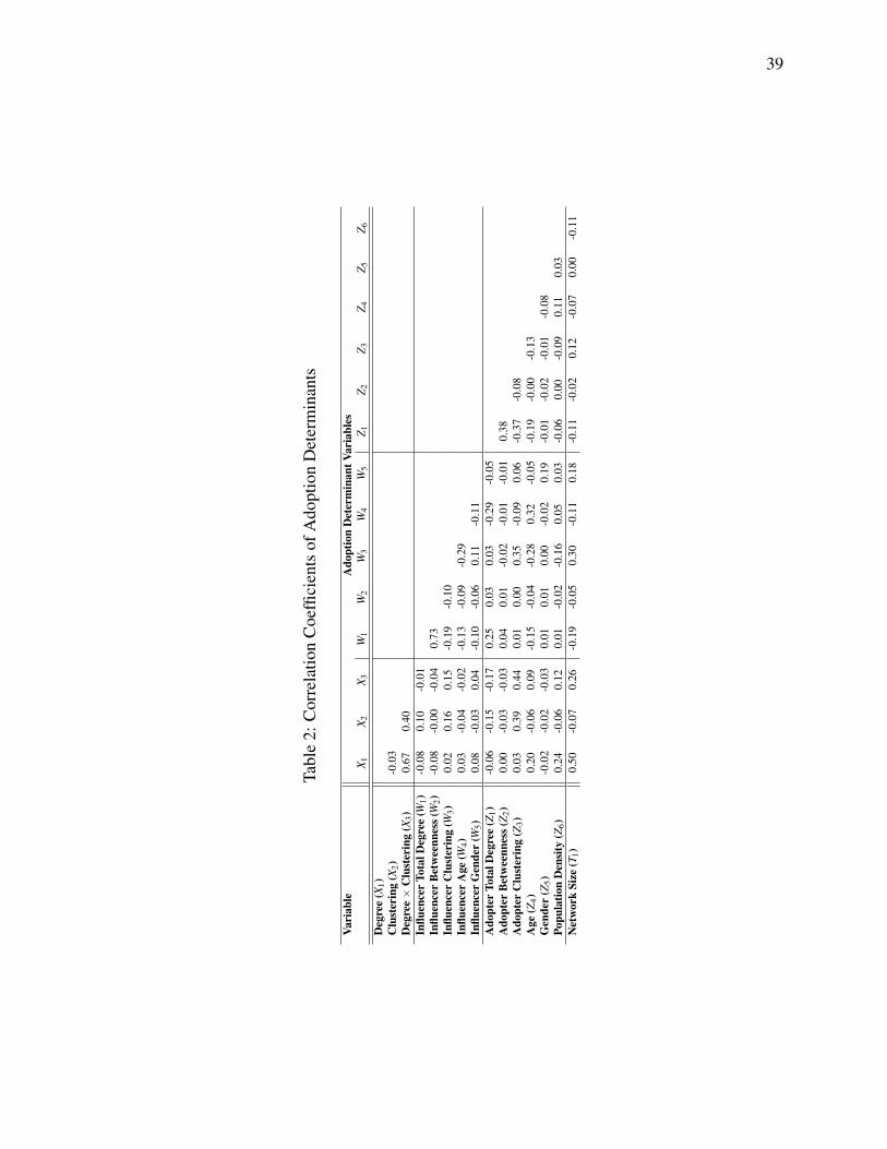
39

Tabl

e2:

Cor

rela

tion

Coe

ffici

ents

ofA

dopt

ion

Det

erm

inan

ts

Vari

able

Ado

ptio

nD

eter

min

antV

aria

bles

X 1X 2

X 3W

1W

2W

3W

4W

5Z 1

Z 2Z 3

Z 4Z 5

Z 6D

egre

e(X

1)C

lust

erin

g(X

2)-0

.03

Deg

ree×

Clu

ster

ing

(X3)

0.67

0.40

Influ

ence

rTo

talD

egre

e(W

1)-0

.08

0.10

-0.0

1In

fluen

cer

Bet

wee

nnes

s(W

2)-0

.08

-0.0

0-0

.04

0.73

Influ

ence

rC

lust

erin

g(W

3)0.

020.

160.

15-0

.19

-0.1

0In

fluen

cer

Age

(W4)

0.03

-0.0

4-0

.02

-0.1

3-0

.09

-0.2

9In

fluen

cer

Gen

der

(W5)

0.08

-0.0

30.

04-0

.10

-0.0

60.

11-0

.11

Ado

pter

Tota

lDeg

ree

(Z1)

-0.0

6-0

.15

-0.1

70.

250.

030.

03-0

.29

-0.0

5A

dopt

erB

etw

eenn

ess(

Z 2)

0.00

-0.0

3-0

.03

0.04

0.01

-0.0

2-0

.01

-0.0

10.

38A

dopt

erC

lust

erin

g(Z

3)0.

030.

390.

440.

010.

000.

35-0

.09

0.06

-0.3

7-0

.08

Age

(Z4)

0.20

-0.0

60.

09-0

.15

-0.0

4-0

.28

0.32

-0.0

5-0

.19

-0.0

0-0

.13

Gen

der

(Z5)

-0.0

2-0

.02

-0.0

30.

010.

010.

00-0

.02

0.19

-0.0

1-0

.02

-0.0

1-0

.08

Popu

latio

nD

ensi

ty(Z

6)0.

24-0

.06

0.12

0.01

-0.0

2-0

.16

0.05

0.03

-0.0

60.

00-0

.09

0.11

0.03

Net

wor

kSi

ze(T

1)0.

50-0

.07

0.26

-0.1

9-0

.05

0.30

-0.1

10.

18-0

.11

-0.0

20.

12-0

.07

0.00

-0.1

1

40

Table 3: Parameter Estimates of Different Model Specifications

Probability of Adoption Model 1 Model 2 Model 3 Model 2b Model 3bMean Mean Mean Mean Mean

(z-value) (z-value) (z-value) (z-value) (z-value)

Degree 4.476∗∗∗ 4.383∗∗∗ 4.476∗∗∗ 4.401∗∗∗ 4.483∗∗∗

(215.95) (183.41) (114.27) (182.90) (114.21)Network Clustering 0.361∗∗∗ 0.689∗∗∗ 0.704∗∗∗ 0.703∗∗∗ 0.713∗∗∗

Effects (18.02) (32.48) (24.89) (33.06) (25.16)Degree × Clustering -1.916∗∗∗ 0.552∗∗∗ 1.305∗∗∗ 0.492∗∗∗ 1.274∗∗∗

(-43.31) (7.33) (10.00) (6.50) (9.76)

Avg. Total Degree -0.00075∗∗∗ -0.00090∗∗∗ -0.00079∗∗∗ -0.00092∗∗∗

(-17.50) (-15.64) (-18.18) (-15.91)

Avg. (Total Degree)2 0.000020 0.000027∗

(×0.001) (1.86) (2.27)Avg. Betweenness -0.0067 0.00025 -0.000075 -0.0000013(×0.001) (-1.88) (0.59) (-1.89) (-0.03)

Influencer Avg. Clustering 3.867∗∗∗ 4.269∗∗∗ 3.777∗∗∗ 4.197∗∗∗

Effects (28.48) (21.22) (27.70) (20.82)Avg. Age -0.0082∗∗∗ -0.0082∗∗∗

(-7.24) (-7.24)Gender 0.076∗∗∗ 0.077∗∗∗

(Fraction of females) (3.57) (3.62)

Total Degree 0.0010∗∗∗ 0.0011∗∗∗ 0.0012∗∗∗ 0.0013∗∗∗

(39.02) (34.78) (33.57) (27.63)

(Total Degree)2 -0.00027∗∗∗ -0.00020∗∗∗

(×0.001) (-6.95) (-3.98)Betweenness -0.00022∗∗∗ -0.00020∗∗∗ 0.000066 -0.000016(×0.001) (-7.02) (-5.44) (1.77) (-0.33)Clustering -2.614∗∗∗ -3.322∗∗∗ -2.548∗∗∗ -3.266∗∗∗

Adopter (-40.86) (-34.38) (-39.52) (-33.59)Effects Age 0.0029∗∗∗ 0.0030∗∗∗

(5.89) (6.11)Gender 0.0068 0.0070(Male=0, Female=1) (0.96) (0.98)Population Density 0.0012∗∗∗ 0.0012∗∗∗

(City of residence) (3.97) (4.06)

Network Size 0.013∗∗∗ 0.012∗∗∗ 0.012∗∗∗ 0.012∗∗∗ 0.012∗∗∗

(×0.001) (134.39) (118.44) (92.28) (118.08) (92.18)Const. -8.830∗∗∗ -8.896∗∗∗ -8.903∗∗∗ -8.922∗∗∗ -8.925∗∗∗

(-1029.77) (-455.45) (-183.19) (-450.13) (-182.36)

Observations 188,631,660 188,628,849 136,829,184 188,628,849 136,829,184Pseudo R2 0.0455 0.0487 0.0496 0.0487 0.0496∗p < .05, ∗∗p < .01, ∗∗∗p < .001

41

Table 4: Comparing model fit over the same set of observations

Probability of Adoption Model 1 Model 2 Model 3Mean Mean Mean(z-value) (z-value) (z-value)

Degree 4.929∗∗∗ 4.535∗∗∗ 4.476∗∗∗

(154.49) (120.68) (114.27)

Network Clustering 0.363∗∗∗ 0.690∗∗∗ 0.704∗∗∗

Effects (13.51) (24.47) (24.89)

Degree × Clustering -2.144∗∗∗ 1.312∗∗∗ 1.305∗∗∗

(-22.88) (10.06) (10.00)

Avg. Total Degree -0.00087∗∗∗ -0.00090∗∗∗

(-15.57) (-15.64)

Avg. Betweenness 0.000022 0.000025(×0.001) (0.52) (0.59)

Influencer Avg. Clustering 4.516∗∗∗ 4.269∗∗∗

Effects (24.20) (21.22)

Avg. Age -0.0082∗∗∗

(-7.24)

Gender 0.076∗∗∗

(Fraction of females) (3.57)

Total Degree 0.0011∗∗∗ 0.0011∗∗∗

(34.66) (34.78)

Betweenness -0.00018∗∗∗ -0.00020∗∗∗

(×0.001) (-5.22) (-5.44)

Clustering -3.354∗∗∗ -3.322∗∗∗

Adopter (-34.86) (-34.38)

Effects Age 0.0029∗∗∗

(5.89)

Gender 0.0068(Male=0, Female=1) (0.96)

Population Density 0.0012∗∗∗

(City of residence) (3.97)

Network Size 0.013∗∗∗ 0.012∗∗∗ 0.012∗∗∗

(×0.001) (106.69) (94.59) (92.28)

Const. -8.929∗∗∗ -8.981∗∗∗ -8.903∗∗∗

(-845.80) (-367.65) (-183.19)

Observations 136,829,184 136,829,184 136,829,184Pseudo R2 0.0461 0.0495 0.0496AIC 1,368,561.20 1,363,723.66 1,363,624.20BIC 1,368,644.87 1,363,907.74 1,363,891.95∗p < .05, ∗∗p < .01, ∗∗∗p < .001

42

Table 5: Adoption percentage of predicted adopters

Successful prediction rateNumber of adopters predicted (m) Model 1 Model 2 Model 3 Model 4 Random500 30.60% 29.60% 28.80% 13.60% 11.66%1000 26.80% 27.60% 27.20% 13.40% 11.66%2000 24.45% 24.45% 24.40% 12.35% 11.66%4000 23.15% 23.32% 23.22% 12.10% 11.66%9944 20.71% 21.19% 21.19% 13.25% 11.66%

43

Table 6: Parameter Estimates, Random Effects Complementary Log-log Regression


Degree 31.144∗∗∗ 36.963∗∗∗ 35.655∗∗∗

(59.23) (36.60) (28.82)

Network Clustering 1.275∗∗ 3.013∗∗ 1.400∗∗

Effects (3.41) (3.47) (2.84)


(-10.90) (4.23) (5.46)

Avg. Total Degree -0.012∗∗∗ -0.011∗∗∗

(-9.67) (-7.38)

Avg. Betweenness 0.0054∗∗∗ 0.0040∗∗∗

(×0.001) (7.35) (6.81)


Effects (6.33) (4.69)

Avg. Age 0.012(0.59)

Gender 0.145(Fraction of females) (0.34)

Total Degree 0.0088∗∗∗ 0.0081∗∗∗

(4.48) (4.91)

Betweenness 0.0034 0.0064(×0.001) (0.52) (1.66)

Clustering -32.318∗∗∗ -33.609∗∗∗

Adopter (-13.60) (-12.46)

Effects Age 0.027(0.96)


Population Density 0.0054(City of residence) (0.52)

Network Size 0.079∗∗∗ 0.067∗∗∗ 0.088∗∗∗

(×0.001) (45.93) (39.30) (28.52)

Const. -21.543∗∗∗ -22.411∗∗∗ -24.331∗∗∗

(-99.44) (-36.41) (-17.02)

Observations 3,780,234 3,772,389 2,730,623Individuals 4594 4552 3208ρ 0.9741 0.9653 0.9825∗p < .05, ∗∗p < .01, ∗∗∗p < .001

44

Table 7: Parameter Estimates, Correcting for Unobserved Heterogeneity


Degree 4.476∗∗∗ 4.383∗∗∗ 4.476∗∗∗

(10.01) (11.54) (12.53)


Effects (7.43) (25.18) (70.19)

Degree × Clustering -1.916∗∗∗ 0.552∗∗ 1.305(-5.06) (2.68) (1.69)

Avg. Total Degree -0.00075∗∗ -0.00090∗∗∗

(-3.40) (-5.53)

Avg. Betweenness -0.0067 0.00025(×0.001) (-1.86) (0.66)


Effects (11.31) (9.04)

Avg. Age -0.0082∗

(-2.39)


Total Degree 0.0010∗∗∗ 0.0011∗∗∗

(10.35) (20.11)

Betweenness -0.00022∗∗∗ -0.00020∗∗∗

(×0.001) (-8.89) (-3.72)

Clustering -2.614∗∗∗ -3.322∗∗∗

Adopter (-13.30) (-6.28)

Effects Age 0.0029(0.76)


Population Density 0.0012∗∗


Network Size 0.013∗∗∗ 0.012∗∗∗ 0.012∗∗∗

(×0.001) (4.19) (4.20) (4.91)

Const. -8.830∗∗∗ -8.896∗∗∗ -8.903∗∗∗

(-27.25) (-31.45) (-25.46)

Observations 188,631,660 188,628,849 136,829,184Pseudo R2 0.0455 0.0487 0.0496∗p < .05, ∗∗p < .01, ∗∗∗p < .001

45

Tabl

e8:

Para

met

erE

stim

ates

with

With

in-C

ityN

etw

orks

Con

side

red

(Mod

els

5an

d6)

Prob

abili

tyof

Ado

ptio

nM

odel

5M

odel

6M

ean

z-va

lue

Mea

nz-

valu

eD

egre

e,W

ithin

-City

2.73

1∗∗∗

103.

352.

226∗∗∗

97.0

5N

etw

ork

Deg

ree,

Acr

oss-

Citi

es0.

070∗∗∗

4.65

-0.0

0084

-0.0

6E

ffec

tsC

lust

erin

g0.

588∗∗∗

16.3

50.

129∗∗∗

4.10

Deg

ree×

Clu

ster

ing

6.02

7∗∗∗

57.0

5D

egre

e,W

ithin

-City×

Clu

ster

ing

-0.0

67-0

.77

Avg

.Tot

alD

egre

e,W

ithin

-City

-0.0

0034∗∗∗

-6.7

3-0

.000

40∗∗∗

-7.8

4A

vg.T

otal

Deg

ree,

Acr

oss-

Citi

es0.

0000

841.

940.

0000

481.

17In

fluen

cer

Avg

.Bet

wee

nnes

s,W

ithin

-City

(×0.

001)

-0.0

0037∗∗∗

-7.2

5-0

.000

27∗∗∗

-5.5

9E

ffec

tsA

vg.B

etw

eenn

ess,

Acr

oss-

Citi

es(×

0.00

1)-0

.000

23∗∗

-2.6

4-0

.000

13-1

.57

Avg

.Clu

ster

ing

3.06

7∗∗∗

14.4

44.

354∗∗∗

21.9

4A

vg.A

ge-0

.017∗∗∗

-14.

87-0

.016∗∗∗

-13.

34G

ende

r(fr

actio

nof

fem

ales

)0.

010

0.47

0.06

3∗∗

2.81

Tota

lDeg

ree

0.00

14∗∗∗

40.6

40.

0011∗∗∗

32.4

7B

etw

eenn

ess

(×0.

001)

-0.0

0042∗∗∗

-8.3

3-0

.000

25∗∗∗

-5.8

2A

dopt

erC

lust

erin

g-1

.520∗∗∗

-17.

52-4

.493∗∗∗

-46.

35E

ffec

tsA

ge0.

0030∗∗∗

6.02

0.00

15∗∗

2.90

Gen

der

0.00

841.

150.

0072

0.99

Popu

latio

nD

ensi

ty(c

ityof

resi

denc

e)0.

0073∗∗∗

23.1

30.

0035∗∗∗

10.8

7N

etw

ork

Size

,With

in-C

ity(×

0.00

1)-0

.008

8∗∗∗

-52.

45-0

.008

7∗∗∗

-50.

97N

etw

ork

Size

,Acr

oss-

Citi

es(×

0.00

1)0.

087∗∗∗

253.

590.

087∗∗∗

259.

41C

onst

.-8

.733∗∗∗

-182

.87

-8.3

12∗∗∗

-174

.60

Obs

erva

tions

118,

612,

170

118,

612,

170

Pseu

doR

20.

0582

0.06

03∗∗∗ p

<.0

01,∗∗ p

<.0

1,∗ p

<.0

5

46

Table 9: Parameter Estimates, Non-normalized Degree


Degree 0.0071∗∗∗ 0.011∗∗∗ 0.0088∗∗∗

(96.95) (96.84) (61.27)


Effects (33.25) (17.17) (18.69)

Degree × Clustering 0.019∗∗∗ 0.017∗∗∗ 0.020∗∗∗

(40.20) (29.83) (28.34)

Avg. Total Degree -0.00088∗∗∗ -0.00065∗∗∗

(-19.82) (-11.13)

Avg. Betweenness -0.000070 -0.00016∗∗

(×0.001) (-1.96) (-3.47)

Influencer Avg. Clustering -1.808∗∗∗ 0.532∗

Effects (-11.29) (2.32)

Avg. Age -0.0092∗∗∗

(-8.35)


Total Degree -0.0015∗∗∗ -0.0010∗∗∗

(-44.84) (-23.98)

Betweenness 0.00014∗∗ 0.00014∗∗∗

(×0.001) (3.18) (4.00)

Clustering 0.664∗∗∗ -1.803∗∗∗

Adopter (16.00) (-20.95)


(17.95)


Population Density 0.0059∗∗∗


Network Size 0.016∗∗∗ 0.013∗∗∗ 0.016∗∗∗

(×0.001) (170.14) (131.62) (122.57)

Const. -8.768∗∗∗ -7.964∗∗∗ -8.425∗∗∗

(-1069.21) (-374.62) (-169.13)


47

Table 10: Uniformity of Network Growth

Percentage Growth of Personal Network Coefficient z-valueDuring Two Years (748 Days) After SamplingDay Joined -0.0000025 -0.11Number of Friends in Sample -0.19 -0.99Const. 55.53 1.95∗p < .05 Number of observations: 93. F(2,90) = 0.49.

48

Table 11: Parameter Estimates of Different Model Specifications for the First 138,964 Adopters


Degree 2.554∗∗∗ 2.481∗∗∗ 2.151∗∗∗

(102.58) (90.66) (49.72)


Effects (20.84) (30.91) (25.10)


(-22.26) (8.06) (11.06)

Avg. Total Degree -0.0011∗∗∗ -0.0011∗∗∗

(-25.55) (-18.70)

Avg. Betweenness 0.00027∗∗∗ 0.00022∗∗∗

(×0.001) (8.59) (5.65)


Effects (20.00) (13.07)

Avg. Age -0.0062∗∗∗

(-5.32)

Gender 0.130∗∗∗

(Fraction of females) (5.92)

Total Degree 0.00054∗∗∗ 0.00068∗∗∗

(21.53) (21.15)

Betweenness -0.000030 -0.000086∗∗

(×0.001) (-1.47) (-2.91)

Clustering -1.898∗∗∗ -2.540∗∗∗

Adopter (-30.75) (-26.88)


(11.25)

Gender -0.033∗∗∗

(Male=0, Female=1) (-4.58)

Population Density -0.00056(City of residence) (-1.87)

Network Size 0.027∗∗∗ 0.026∗∗∗ 0.028∗∗∗

(×0.001) (261.41) (237.42) (191.56)

Const. -8.553∗∗∗ -8.372∗∗∗ -8.489∗∗∗

(-953.97) (-425.88) (-170.33)


49

Tabl

e12

:Par

amet

erE

stim

ates

forC

onde

nsed

Frie

ndsh

ipN

etw

orks

Frie

ndsA

dopt

ing

with

in60

Day

sFr

iend

sAdo

ptin

gw

ithin

30D

ays

Prob

abili

tyof

Ado

ptio

nM

odel

1M

odel

2M

odel

3M

odel

1M

odel

2M

odel

3M

ean

Mea

nM

ean

Mea

nM

ean

Mea

n(z

-val

ue)

(z-v

alue

)(z

-val

ue)

(z-v

alue

)(z

-val

ue)

(z-v

alue

)

Deg

ree

3.74

2∗∗∗

3.68

2∗∗∗

3.80

9∗∗∗

3.06

6∗∗∗

2.81

3∗∗∗

2.85

7∗∗∗

(258

.07)

(214

.03)

(184

.80)

(195

.11)

(148

.92)

(127

.96)

Net

wor

kC

lust

erin

g0.

287∗∗∗

0.21

9∗∗∗

0.16

3∗∗∗

0.31

6∗∗∗

0.12

8∗∗∗

0.06

8∗∗

Eff

ects

(15.

68)

(11.

40)

(6.9

9)(1

6.11

)(6

.26)

(2.7

8)

Deg

ree×

Clu

ster

ing

-0.7

58∗∗∗

-0.7

95∗∗∗

-0.7

22∗∗∗

-0.6

58∗∗∗

-0.7

39∗∗∗

-0.5

83∗∗∗

(-24

.62)

(-17

.37)

(-12

.70)

(-20

.79)

(-16

.39)

(-10

.55)

Avg

.Tot

alD

egre

e-0

.002

2∗∗∗

-0.0

021∗∗∗

0.00

49∗∗∗

0.00

54∗∗∗

(-9.

74)

(-7.

78)

(12.

85)

(11.

91)

Avg

.Bet

wee

nnes

s0.

037∗∗∗

0.03

8∗∗∗

-0.0

38∗∗∗

-0.0

41∗∗∗

(×0.

001)

(19.

24)

(17.

03)

(-8.

30)

(-7.

59)

Influ

ence

rA

vg.C

lust

erin

g0.

700∗∗∗

0.64

9∗∗∗

0.51

5∗∗∗

0.48

3∗∗∗

Eff

ects

(16.

73)

(12.

39)

(14.

47)

(11.

10)

Avg

.Age

0.00

050

-0.0

0053

(0.7

1)(-

0.72

)

Gen

der

-0.0

99∗∗∗

-0.1

00∗∗∗

(Fra

ctio

nof

fem

ales

)(-

7.10

)(-

7.03

)

Tota

lDeg

ree

0.00

0024

0.00

033

-0.0

039∗∗∗

-0.0

038∗∗∗

(0.1

3)(1

.66)

(-10

.54)

(-8.

86)

Bet

wee

nnes

s-0

.022∗∗∗

-0.0

22∗∗∗

-0.0

80∗∗∗

-0.0

80∗∗∗

(×0.

001)

(-14

.42)

(-13

.07)

(-19

.96)

(-17

.62)

Clu

ster

ing

0.00

310.

031

0.20

9∗∗∗

0.18

7∗∗∗

Ado

pter

(0.0

9)(0

.77)

(6.7

6)(4

.95)

Eff

ects

Age

0.00

079

-0.0

015∗∗

(1.4

5)(-

2.47

)

Gen

der

-0.0

046

-0.0

013

(Mal

e=0,

Fem

ale=

1)(-

0.60

)(-

0.16

)

Popu

latio

nD

ensi

ty0.

0021∗∗∗

0.00

14∗∗∗

(City

ofre

side

nce)

(6.4

3)(3

.87)

Net

wor

kSi

ze0.

0026∗∗∗

0.00

26∗∗∗

0.00

30∗∗∗

-0.0

0028∗∗

0.00

20∗∗∗

0.00

23∗∗∗

(×0.

001)

(29.

19)

(26.

55)

(24.

28)

(-3.

01)

(19.

33)

(18.

15)

Con

st.

-5.2

93∗∗∗

-5.3

17∗∗∗

-5.4

18∗∗∗

-4.1

20∗∗∗

-4.1

64∗∗∗

-4.1

25∗∗∗

(-47

4.07

)(-

358.

38)

(-17

5.02

)(-

333.

52)

(-25

8.03

)(-

127.

72)

Obs

erva

tions

5,07

8,03

55,

053,

555

3,71

8,55

11,

817,

996

1,79

5,12

11,

322,

861

Pseu

doR

20.

0863

0.08

750.

0882

0.08

400.

0912

0.09

17∗

p<

.05,∗∗

p<

.01,∗∗∗

p<

.001

50

Tabl

e13

:Par

amet

erE

stim

ates

forM

odel

sC

onsi

deri

ngon

lya

Bou

nded

Num

bero

fAdo

ptio

nD

ecis

ions

Firs

t60

Ado

ptio

nD

ecis

ions

Con

side

red

Firs

t30

Ado

ptio

nD

ecis

ions

Con

side

red

Prob

abili

tyof

Ado

ptio

nM

odel

1M

odel

2M

odel

3M

odel

1M

odel

2M

odel

3M

ean

Mea

nM

ean

Mea

nM

ean

Mea

n(z

-val

ue)

(z-v

alue

)(z

-val

ue)

(z-v

alue

)(z

-val

ue)

(z-v

alue

)

Deg

ree

4.68

6∗∗∗

4.00

6∗∗∗

4.57

3∗∗∗

4.89

0∗∗∗

3.40

0∗∗∗

3.78

7∗∗∗

(35.

30)

(27.

23)

(14.

71)

(20.

57)

(12.

48)

(4.8

8)

Net

wor

kC

lust

erin

g0.

739∗∗∗

0.66

6∗∗∗

0.69

6∗∗∗

1.25

1∗∗∗

0.95

1∗∗∗

0.97

4∗∗∗

Eff

ects

(13.

16)

(11.

68)

(8.9

0)(1

3.83

)(1

0.22

)(7

.65)

Deg

ree×

Clu

ster

ing

-1.1

88∗∗∗

0.08

71.

465∗

-1.5

02∗∗∗

-0.5

22-0

.080

(-7.

67)

(0.3

1)(2

.46)

(-5.

84)

(-1.

35)

(-0.

08)

Avg

.Tot

alD

egre

e-0

.001

6∗∗∗

-0.0

012∗∗∗

-0.0

028∗∗∗

-0.0

026∗∗∗

(-7.

90)

(-4.

03)

(-8.

89)

(-5.

23)

Avg

.Bet

wee

nnes

s0.

0002

30.

0001

40.

0009

4∗∗

0.00

11∗∗

(×0.

001)

(0.9

3)(0

.40)

(2.6

6)(3

.22)

Influ

ence

rA

vg.C

lust

erin

g1.

763∗∗∗

3.86

6∗∗∗

1.46

0∗∗

2.66

1E

ffec

ts(4

.11)

(4.0

3)(2

.99)

(1.9

1)

Avg

.Age

-0.0

022

-0.0

014

(-0.

50)

(-0.

19)

Gen

der

0.01

90.

058

(Fra

ctio

nof

fem

ales

)(0

.19)

(0.3

8)

Tota

lDeg

ree

-0.0

021∗∗∗

-0.0

0027

-0.0

064∗∗∗

-0.0

027∗∗∗

(-9.

30)

(-0.

92)

(-13

.05)

(-4.

11)

Bet

wee

nnes

s0.

0005

8∗∗∗

0.00

0089

0.00

22∗∗

-0.0

028

(×0.

001)

(5.7

6)(0

.15)

(2.7

8)(-

0.55

)

Clu

ster

ing

-1.2

62∗∗∗

-3.5

21∗∗∗

-0.6

86∗

-2.2

21∗∗

Ado

pter

(-5.

19)

(-6.

73)

(-2.

39)

(-3.

15)

Eff

ects

Age

0.02

9∗∗∗

0.02

0∗∗∗

(11.

76)

(4.0

1)

Gen

der

-0.3

98∗∗∗

-0.2

36∗

(Mal

e=0,

Fem

ale=

1)(-

6.55

)(-

2.22

)

Popu

latio

nD

ensi

ty0.

0096∗∗∗

0.00

15(C

ityof

resi

denc

e)(3

.67)

(0.3

5)

Net

wor

kSi

ze0.

013∗∗∗

0.00

83∗∗∗

0.01

7∗∗∗

0.01

7∗∗∗

0.00

88∗∗∗

0.02

0∗∗∗

(×0.

001)

(14.

79)

(8.5

7)(9

.56)

(16.

77)

(7.8

7)(9

.80)

Con

st.

-8.3

11∗∗∗

-7.2

16∗∗∗

-8.7

75∗∗∗

-8.4

33∗∗∗

-6.2

67∗∗∗

-7.5

97∗∗∗

(-23

7.15

)(-

76.6

0)(-

36.7

9)(-

119.

31)

(-42

.14)

(-17

.73)

Obs

erva

tions

4,55

3,57

94,

553,

526

3,26

5,04

81,

185,

452

1,18

5,43

084

0,97

3Ps

eudo

R2

0.07

180.

0793

0.04

060.

1353

0.16

370.

0841

∗p

<.0

5,∗∗

p<

.01,∗∗∗

p<

.001

Documents

Network Effects and Personal Influences: The Diffusion of an Online