^"V.

^^

Dewey

WORKING PAPER

ALFRED P. SLOAN SCHOOL OF MANAGEMENT

NETWORK FLOWS

Ravindra K. AhujaThomas L. MagnantiJames B. Orlin

Sloan W.P. No. 2059-88August 1988

Revised: December, 1988

MASSACHUSETTS

INSTITUTE OF TECHNOLOGY50 MEMORIAL DRIVE

CAMBRIDGE, MASSACHUSETTS 02139

NETWORK FLOWS

Ravindra K. AhujaThomas L. MagnantiJames B. Orlin

August 1988

Sloan W.P. No. 2059-88 Revised: December, 1988

NETWORK FLOWS

Ravindra K. Ahuja* , Thomas L. Magnanti, and James B. Orlin

Sloan School of ManagementMassachusetts Institute of Technology

Cambridge, MA. 02139

On leave from Indian Institute of Technology, Kanpur - 208016, INDIA

MIT. LffiRARF

JUN 1 --^

NETWORK FLOWS

OVERVIEW

Introduction1.1 Applications1.2 Complexity Analysis

1.3 Notation and Definitions

1.4 Network Representations1.5 Search Algorithms1.6 Developing Polynomial Time Algorithms

Basic Properties of Network Flows21 Flow Decomposition Properties and Optimality ConditionsZ2 Cycle Free and Spanning Tree Solutions

Z3 Networks, Linear and Integer Programming24 Network Transformations

Shortest Paths3.1 Dijkstra's Algorithm3.2 Dial's Implementation3.3 R-Heap Implementation3.4 Label Correcting Algorithms3.5 All Pairs Shortest Path Algorithm

Maximum Flows4.1 Labeling Algorithm and the Max-Flow Min-Cut Theorem4.2 Decreasing the Number of Augmentations4.3 Shortest Augmenting Path Algorithm4.4 Preflow-Push Algorithms4.5 Excess-Scaling Algorithm

Minimum Cost Flows5.1 Duality and Optimality Conditions5.2 Relationship to Shortest Path and Maximum Flow Problems5.3 Negative Cycle Algorithm5.4 Successive Shortest Path Algorithm5.5 Primal-Dual and Out-of-Kilter Algorithnns5.6 Network Simplex Algorithm5.7 Right-Hand-Side Scaling Algorithm5.8 Cost Scaling Algorithm5.9 Double Scaling Algorithm5.10 Sensitivity Analysis5.11 Assignment Problem

Reference Notes

References

Network Flows

Perhaps no subfield of mathematical programming is more alluring than

network optimization. Highway, rail, electrical, communication and many other

physical networks pervade our everyday lives. As a consequence, even non-specialists

recognize the practical importance and the wide ranging applicability of networks.

Moreover, because the physical operating characteristics of networks (e.g., flows on arcs

and mass balance at nodes) have natural mathematical representations, practitioners and

non-specialists can readily understand the mathematical descriptions of network

optimization problems and the basic ruiture of techniques used to solve these problems.

This combination of widespread applicability and ease of assimilation has undoubtedly

been instrumental in the evolution of network planning models as one of the most

widely used modeling techniques in all of operatior^s research and applied mathematics.

Network optimization is also alluring to methodologists. Networks provide a

concrete setting for testing and devising new theories. Indeed, network optimization has

inspired many of the most fundamental results in all of optimization. For example,

price directive decomposition algorithms for both linear programming and

combinatorial optimization had their origins in network optimization. So did cutting

plane methods and branch and bound procedures of integer programming, primal-dual

methods of linear and nonlinear programming, and polyhedral methods of

combinatorial optimization. In addition, networks have served as the major prototype

for several theoretical domaiiis (for example, the field of matroids) and as the core model

for a wide variety of min/max duality results in discrete mathematics.

Moreover, network optimization has served as a fertile meeting ground for ideas

from optimization and computer science. Many results in network optimization are

routinely used to design and evaluate computer systems, and ideas from computer

science concerning data structures and efficient data manipulation have had a major

impact on the design and implementation of many network optimization algorithms.

The aim of this paf>er is to summarilze many of the fundamental ideas of network

optimization. In particular, we concentrate on network flow problems and highlight a

number of recent theoretical and algorithmic advances. We have divided the discussion

into the following broad major topics:

Applications

Basic Prof)erties of Network Flows

Shortest Path Problems''

Maximum Flow Problems

Minimum Cost Flow Problems

AssigTunent Problems

Much of our discussion focuses on the design of provably good (e.g.,

polynomial-time) algorithms. Among good algorithms, we have presented those that

are simple and are likely to be efficient in practice. We have attempted to structure our

discussion so that it not only provides a survey of the field for the specialists, but also

serves as an introduction and summary to the non-specialists who have a basic working

knowledge of the rudiments of optimization, particularly linear programming.

In this chapter, we limit our discussions to the problems listed above. Some

important generalizations of these problems such as (i) the generalized network flows;

(ii) the multicommodity flows; and (iv) the network design, will not be covered in our

survey. We, however, briefly describe these problems in Section 6.6 and provide some

important references.

As a prelude to the remainder of our discussion, in this section we present

several important preliminaries . We discuss (i) different ways to measure the

performance of algorithms; (ii) graph notation and vtirious ways to represent networks

quantitively; (iii) a few basic ideas from computer science that underUe the design of

many algorithms; and (iv) two generic proof techniques that have proven to be useful

in designing polynomial-time algorithms.

1.1 Applications

Networks arise in numerous application settings emd in a variety of guises. In

this section, we briefly describe a few prototypical applications. Our discussion is

intended to illustrate a range of applications and to be suggestive of how network flow

problems arise in practice; a more extensive survey would take us far beyond the scope

of our discussion. To illustrate the breadth of network applications, we consider some

models requiring solution techniques that we will not describe in this chapter.

For the purposes of this discussion, we will consider four different types of

networks arising in practice:

• Physical networks (Streets, railbeds, pipelines, wires)

• Route networks

• Space-time networks (Scheduling networks)

• Derived networks (Through problem trai^formations)

These four categories are not exhaustive and overlap in coverage. Nevertheless,

they provide a useful taxonomy for summarizing a variety of applications.

Network flow models are also used for several purposes:

• Descriptive modeling (answering "what is?" questions)

• Predictive modeling (answering "what will be?" questions)

• Normative modeling (answering "what should be?" questions, that is,

performing optimization)

We will illustrate models in each of these categories. We first introduce the basic

underlying network flow model and some useful notation.

The Network Flow Model

Let G = (N, A) be a directed network with a cost Cjj, a lower bound /,;, and a

capacity Uj; associated with every arc (i, j) e A. We associate with each node i e N an

integer number b(i) representing its supply or demand. If b(i) > 0, then node i is a supply

node; if b(i) < 0, then node i is a demand node; and if b(i) = 0, then node i is a transhipment

node. Let n =| N |

and m =| A |. The minimum cost network flow problem can be

formulated as follows:

Minimize ^ C;; x;: (1.1a)

(i,j)€A^'

subject to

X^ii - Xxji =b(i), foralli€N, (1.1b)

{j:(i,j)e]\} {j:(j,i)6^A}

/jj< Xjj S u^ . for all (i, j) e A. (1 .Ic)

We refer to the vector x = (xjj) as the flow in the network. The constraint (1.1b)

implies that the total flow out of a node minus the total flow into that node must equal

the net supply /demand of the node. We henceforth refer to this constraint as the moss

balance constraint. The flow must also satisfy the lower bound and capacity constraints

(1.1c) which we refer to as the flow bound constraints. The flow bounds might model

physical capacities, contractual obligations or simply operating ranges of interest.

Frequently, the given lower bounds /j; are all zero; we show later that they can be made

zero without any loss of generality.

In matrix notation, we represent the minimum cost flow problem

minimize { ex : Nx = b and / < x S u ), (1.2)

in terms of a node-arc incidence matrix N. The matrix N has one row for each node of the

network and one column for each arc. We let Njj represent the column of Ncorresponding to arc (i, j), and let e; denote the j-th unit vector which is a column vector

of size n whose entries are all zeros except for the )-th entry which is a 1. Note that each

flow variable x-; app>ears in two mass balance equations, as an outflow from node i with

a +1 coefficient and as an inflow to node j with a -1 coefficient. Therefore the column

corresponding to arc (i, j) is Nj; = Cj - e;

.

The matrix N has very special structure: only 2m out of its nm total entries are

nonzero, all of its nonzero entries are +1 or -1, and each column h<is exactly one +1 and

one -1. Figure 1.1 gives an example of the node-arc incidence matrix. Later in Sections

2.2 and 2.3, we consider some of the consequences of this special structure. For now, we

make two observations.

(i) Summing all the mass balance constraints eliminates all the flow variables and

gives

I b(i) = 0,or Ib(i) = Ib(i) .

i € N i € {N : Mi) > 0) i € {N : b(i) < 0)

Consequently, total supply must equal total demand if the mass balance

cor\straints are to have any feasible solution.

(ii) If the total supply does equal the total demand, then summing all the mass

balance equations gives the zero equation Ox = 0, or equivalently, any equation is

equal to minus the sum of all other equations, and hence is redundant.

The following special ccises of the minimum cost flow problem play a central role in the

theory and applications of network flows.

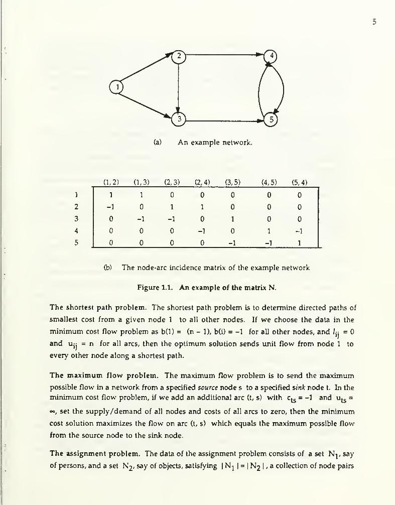
(a) An example network.

1

2

3

4

5

(1,2)

A c Nj X N2 representing possible person-to-object assignments, and a cost C;;

associated with each element (i, j) in A. The objective is to assign each person to exactly

one object in a way that minimizes the cost of the assignment. The Jissignment problem

is a minimum cost flow problem on a network G = (N^ u N2, A) with b(i) = 1 for all i

e Nj and b(i) = -1 for all i e N2 (we set l^:= and u^; = 1 for all (i, j) € A).

Physical Networks"^

The familiar city street map is perhaps the prototypical physical network, and the

one that most readily comes to inind when we envision a network. Many network

planning problems arise in this problem context. As one illustration, consider the

problem of managing, or designing, a street network to decide upon such issues as speed

limits, one way street assignments, or whether or not to construct a new road or bridge.

In order to make these decisions intelligently, we need a descriptive model that tells us

how to model traffic flows and measure the performance of any design as well as a

predictive model for measuring the effect of any change in the system. We can then use

these models to answer a variety of "what if planning questions.

The following type of equilibrium network flow model permits us to answer

these types of questions. Each line of the network has an associated delay function that

specifies how long it takes to traverse this link. The time to do so depends upon traffic

conditions; the more traffic that flows on the link, the longer is the travel time to

traverse it. Now also suppose that each user of the system has a point of origin (e.g., his

or her home) and a point of destination (e.g., his or her workplace in the central

business district). Each of these users must choose a route through the network. Note,

however, that these route choices affect each other; if two users traverse the same link,

they add to each other's travel time because of the added congestion on the link. Now let

us make the behavioral assumption that each user wishes to travel between his or her

origin and destination as quickly as possible, that is, along a shortest travel time path.

This situation leads to the following equilibrium problem vdth an embedded set of

network optimization problems (shortest path problems); is there a flow pattern in the

network with the property that no user can unilaterally change his (or her) choice of

origin to destination path (that is, all other ULsers continue to use their specified paths in

the equilibrium solution) to reduce his travel time. Operations researchers have

developed a set of sophisticated models for this problem setting, as well as related theory

(concerning, for example, existence and uniqueness of equilibrium solutions), and

algorithms for computing equilibrium solutions. Used in the mode of "what if

scenario analysis, these models permit analysts to answer the type of questions we posed

previously. These models are actively used in practice. Indeed, the Urban Mass Transit

Authority in the United States requires that communities perform a network

equilibrium impact analysis as part of the process for obtaining federal funds for highway

construction or improvement.

Similar types of models arise in many other problem contexts. For example, a

network equilibrium model forms the heairt of the Project Independence Energy Systems

(LPIES) model developed by the U.S. Department of Energy as an analysis tool for

guiding public policy on energy. The basic equilibrium model of electrical networks is

another example. In this setting. Ohm's Law serves as the analog of the congestion

function for the traffic equilibrium problem, and Kirkhoffs Law represents the network

mass balance equations.

Another type of physical network is a very large-scale integrated circuit (VLSI

circuit). In this setting the nodes of the network correspond to electrical components

and the links correspond to wires that connect these links. Numerous network

planning problems arise in this problem context. For example, how can we lay out , or

design, *.he smallest possible integrated circuit to make the necessary connections

between its components and maintain necessary sejjarations between the wires (to avoid

electrical interference).

Route Networks

Route networks, which are one level of abstraction removed from physical

networks, are familiar to most students of operations research and management science.

The traditional operations research transportation problem is illustrative. A shipper

with supplies at its plants must ship to geographically dispersed retail centers, each with

a given aistomer demand. Each arc connecting a supply point to a retail center incurs

costs based upon some physical network, in this case the transportation network. Rather

than solving the problem directly on the physical network, we preprocess the data and

construct transportation routes. Consequently, an arc connecting a supply point and

retail center might correspond to a complex four leg distribution channel with legs

(i) from a plant (by truck) to a rail station, (ii) from the rail station to a rail head

elsewhere in the system, (iii) from the rail head (by truck) to a distribution center, and

(iv) from the distribution center (on a local delivery truck) to the final customer (or even

in some cases just to the distribution center). If we assign the arc with the composite

distribution cost of all the intermediary legs, as well as with the distribution capacity for

this route, this problem becomes a classic network transportation model: find the flows

from plants to customers that minimizes overall costs. This type of model is used in

numerous applications. As but one illustration, a prize winning practice paper written

several years ago described an application of such a network planning system by the

Cahill May Roberts Pharmaceutical Company (of Ireland) to reduce overall distribution

costs by 20%, while improving customer service as well.

Many related problems arise in this type of problem setting, for instance, the

design issue of deciding upon the location of the distribution centers. It is possible to

address this type of decision problem using integer programming methodology for

choosing the distribution sites and network flows to cost out (or optimize flows) for any

given choice of sites; using this approach, a noted study conducted several years ago

permitted Hunt Wesson Foods Corporation to save over $1 million annually.

One special case of the transportation problem merits note — the assignment

problem that we introduced previously in this section. This problem has numerous

applications, particularly in problem contexts such as machine scheduling. In this

application context, we would identify the supply points with jobs to be performed, the

demand points with available machines, and the cost associated with arc (i, j) as the cost

of completing job i on machine j. The solution to the problem specifies the minimum

cost assignment of the jobs to the machines, assuming that each machine has the

capacity to perform only one job.

Space Time Networks

Frequently in practice, we wish to schedule some production or service activity

over time. In these instances it is often convenient to formulate a network flow problem

on a "space—time network" with several nodes representing a particular facility (a

machine, a warehouse, an airport) but at different points in time.

Figure 1.2, which represents a core planning model in production planning, the

economic lot size problem, is an important example. In this problem context, we wish to

meet prescribed demands d^ for a product in each of the T time periods. In each

period, we can produce at level Xj and /or we can meet the demand by drav^g upon

inventory I^ from the previous f)eriod. The network representing this problem has

T + 1 nodes: one node t = 1, 2, . . . , T represents each of the planning periods, and one

node represents the "source" of all production. The flow on arc (0, t) prescribes the

production level Xj in period t, and the flow on arc (t, t + 1) represents the inventory

level I^ to be carried from period t to period t + 1 . The mass balance equation for each

period t models the basic accounting equation: incoming inventory plus production in

that period must equal demand plus final inventory. The mass balance equation for

node indicates that all demand (assuming zero beginning and zero fir\al inventory

over the entire planning period) must be produced in some period t = 1, 2, . . . , T.

Whenever the production and holding costs are linear, this problem is easily solved as a

shortest path problem (for each demand period, we must find the minimum cost path of

production and inventory arcs from node to that demand point). If we impose

capacities on production or inventory, the problem becomes a minimum cost network

flow problem.

Id,

Figure 1^. Network flow model of the economic lot size problem.

One extension of this economic lot sizing problem arises frequently in practice.

Assume that production x^ in any period incurs a fixed cost: that is, whenever we

produce in period t (i.e., x^ > 0), no matter how much or how little, we incur a fixed cost

T^. In addition , we may incur a per unit production cost c^ in period t and a per unit

inventory cost h^ for carrying any unit of inventory from period t to i>eriod t + 1.

Hence, the cost on each arc for this problem is either linear (for inventory carrying arcs)

or linear plus a fixed cost (for production arcs). Consequently, the objective function for

10

the problem is concave. As we indicate in Section 2.2 , any such concave cost network

flow problem always has a special type of optimum solution known as a spanning trees

solution. This problem's spanning tree solution decomposes into disjoint directed paths;

the first arc on each path is a production arc (of the form (0, t)) and each other arc is an

inventory carrying arc. This observation implies the following production property: in the

solution, each time we produce, we produce enough to meet the demand for an integral

number of contiguous periods. Moreover, in no period do we both carry inventory from

the previous period and produce.

The production property permits us to solve the problem very efficiently as a

shortest path problem on an auxiliary network G' defined as follows. The network G'

consists of nodes 1 to T + 1, and for every pair of nodes i and j with i < j, it contains

an arc (i, j). The length of arc (i, j) is equal to the production and inventory cost of

satisfying the demand of the periods from i to j-1. Observe that for every production

schedule satisfying the production property, G' contair\s a directed path in G' from node

1 to node T + 1 of the same objective function veilue and vice-versa. Hence we can

obtain the optimum production schedule by solving a shortest path problem.

Many enhancements of the model are possible, for example (i) the production

facility might have limited production capacity or limited storage for inventory, or

(ii) the production facility might be producing several products that are linked by

common production costs or by changeover cost (for example, we may need to change

dies in an automobile stamping plant when making different types of fenders), or that

share common limited production facilities. In most cases, the enhanced models are

quite difficult to solve (they are NP<omplete), though the embedded network structure

often proves to be useful in designing either heuristic or optimization methods.

Another classical network flow scheduling problem is the airline scheduling problem

used to identify a flight schedule for an airline. In this application setting, each node

represents both a geographical location (e.g., an airport) and a point in time (e.g.. New

York at 10 A.M.). The arcs are of two types: (i) service arcs connecting two airports, for

example New York at 10 A.M. to Boston at 11 A.M.; (ii) layover arcs that permit a plane

to stay at New York from 10 A.M. until 11 A.M. to wait for a later flight, or to wait

overnight at New York from 11 P.M. until 6 A.M. the next morning. If we identify

revenues vdth each service leg, a network flow in this network (with no external supply

or demand) will specify a set of flight plans (circulation of airplanes through the

network). A flow that maximizes revenue will prescribe a schedule for an airline's fleet

11

of planes. The same type of network representation arises in many other dynamic

scheduling applications.

Derived Networks

This category is a "grab bag" of specialized applications and illustrates that

sometimes network flow problems arise in surprising ways from problems that on the

surface might not appear to involve networks. The foUovdng examples illustrate this

point.

Single Duty Crew Scheduling. Figure 1.3 illustrates a number of possible duties for the

drivers of a bus company.

Time Period/Duty Number

12

In this formulation the binary variable x: indicates whether (x; = 1) or not (x; =

0) we select the j-th duty; the matrix A represents the matrix of duties and b is a

column vector whose components are all Vs. Observe that the ones in each column of

A occur in consecutive rows because each driver 's duty contains a single work shift (no

split shifts or work breaks). We show that this problem is a shortest path problem. To

make this identification, we perform the following operations: In (1.2b) subtract each

equation from the equation below it. This transformation does not change the solution

to the system. Now add a redundant equation equal to minus the sums of all the

equations in the revised system. Because of the structure of A, each column in the

revised system will have a single +1 (corresponding to the first hour of the duty in the

column of A) and a single -1 (corresponding to the row in A, or the added row, that Hes

just below the last +1 in the column of A). Moreover, the revised right hand side vector

of the problem will have a +1 in row 1 and a -1 in the last (the appended) row.

Therefore, the problem is to ship one unit of flow from node 1 to node 9 at minimum

cost in the network given in Figure 1.4, which is an instance of the shortest path

problem.

1 unit

Figure 1.4. Shortest path formulation of the single duty scheduling problem.

If instead of requiring a single driver to be on duty in each period, we specify a

number to be on duty in each period, the same transformation would produce a

network flow problem, but in this case the right hand side coefficients (supply and

demands) could be arbitrary. Therefore, the transformed problem would be a general

minimum cost network flow problem, rather than a shortest p)ath problem.

Critical Path Scheduling and Networks Derived from Precedence Conditions

In construction and many other project planning applications, workers need to

complete a variety of tasks that are related by precedence conditions; for example, in

constructing a house, a builder must pour the foundation before framing the house and

complete the framing before beginning to install either electrical or plumbing fixtures.

^5

13

This type of application can be formulated mathematically as follows. Suppose we need

to complete J jobs and that job j (j = 1, 2, . . . , J) requires t: days to complete. We are to

choose the start time S; of each job j so that we honor a set of specified precedence

constraints and complete the overall project as quickly as possible. If we represent the

jobs by nodes, then the precedence constraints can be represented by arcs, thereby giving

us a network. The precedence constraints imply that for each arc (i, j) in the network, the

job j cannot start until job i has been completed. For convenience of notation, we add

two dummy jobs, both with zero processing time: a "start" job to be completed before

any other job can begin and a "completion" job J + 1 that cannot be initiated until we

have completed all other jobs. Let G = (N, A) represent the network corresponding to

this augmented project. Then we vdsh to solve the following optimization problem:

minimize sj^^ - Sq ,

T

subject to

Sj S Sj + tj , for each arc (i , j) e A.

On the surface, this problem, which is a linear program in the variables s: , seems

to bear no resemblance to network optimization. Note, however, that if we move the

variable Sj to the left hand side of the constraint, then each constraint contains exactly

two variables, one with a plus one coefficient and one with a minus one coefficient. The

linear programming dual of this problem has a familiar structure. If we associate a dual

variable xj: with each arc (i, j) , then the dual of this problem is

maximize V t; X;; ,

(i,j)€X^

subject to

^ ^ f -l,ifi =

2^ X:; + 2- Xjj si 0, otherwise, for all i € N{j:(i,j)eA) {j:(j,i)€!^) I l,ifi = J + l

14

15

xj; S 0, for all (i, j) 6 A .

This problem requires us to determine the longest path in the network G from

node to node J + 1 with tj as the arc length of arc (i, j). This longest path has the

following interpretation. It is the longest sequence of jobs needed to fulfill the sp>ecified

precedence conditions. Since delaying any job in this sequence must necessarily delay

the completion of the overall project, this path has become known as the critical path and

the problem has become known as the critical path problem. This model heis become a

principal tool in project management, particularly for managing large-scale corwtruction

projects. The critical path itself is important because it identifies those jobs that require

managerial attention in order to complete the project as quickly as possible.

Researchers and practitioners have enhanced this basic model in several ways.

For example, if resources are available for expediting individual jobs, we could consider

the most efficient use of these resources to complete the overall project as quickly as

possible. Certain versions of this problem can be formulated as minimum cost flow

problems.

The open pit mining problem is another network flow problem that arises from

precedence conditions. Consider the open pit mine shown in Figure 1.5. As shown in

this figure, we have divided the region to be mined into blocks. The provisions of any

given mining technology, and perhaps the geography of the mine, impose restrictions

on how we can remove the blocks: for example, we can never remove a block until we

have removed any block that lies immediately above it; restrictions on the "angle" of

mining the blocks might impose similar precedence conditions. Suppose now that each

block j has an associated revenue n (e.g., the value of the ore in the block minus the

cost for extracting the block) and we wish to extract blocks to maximize overall revenue.

If we let y; be a zero-one variable indicating whether (y^ = 1) or not (y; = 0) we extract

block j, the problem will contain (i) a constraint y; ^ y^ (or, y; - yj S 0) whenever we

need to mine block j before block i, and (ii) an objective function specifying that wewish to maximize total revenue ny; , summed over all blocks j. The dual linear

program (obtained from the linear programming version of the problem (with the

constraints ^ y; < 1, rather than y; = or 1) will be a network flow problem with a

node for each block, a variable for each precedence constraint, and the revenue n as the

demand at node j. This network will also have a dummy "collection node" with

demand equal to minus the sum of the rj's, and an arc connecting it to node j (that is.

16

block j); this arc corresponds to the upper bound constraint y; ^ 1 in the original linear

program. The dual problem is one of finding a network flow that minimizes ths sum of

flows on the arcs incident to node 0.

The critical path scheduling problem and open pit mining problem illustrate one

way that network flow problems arise indirectly. Whenever, two variables in a linear

program are related by a precedence conditions, the variable corresponding to this

precedence constraint in the dual linear program v^ll have a network flow structure. If

the only constraints in the problem are precedence constraints, the dual linear program

will be a network flow problem.

Matrix Rounding of Census Information

The U.S. Census Bureau uses census infonnation to construct millions of tables

for a wide variety of purposes. By law, the Bureau has an obligation to protect the source

of its information and not disclose statistics that can be attributed to any particular

individual. It can attempt to do so by rounding the census information contained in any

table. Consider, for example, the data shown in Figure 1.6(a). Since the upper leftmost

entry in this table is a 1, the tabulated information might disclose information about a

particular individual. We might disguise the information in this table as follows;

round each entry in the table, including the row and column sums, either up or dov^n to

the nearest multiple of three, say, so that the entries in the table continue to add to the

(rounded) row and column sums, and the overall sum of the entries in the new table

adds to a rounded version of the overall sum in the original table. Figure 1.6(b) shows a

rounded version of the data that meets this criterion. The problem can be cast as finding

a feasible flow in a network and can be solved by an application of the maximum flow

algorithm. The network contains a node for each row in the table and one node for each

column. It contains an arc connecting node i (corresponding to row i) and nodej

(corresponding to column j): the flow on this arc should be the ij-th entry in the

prescribed table, rounded either up or dov^T*. In addition, we add a supersource s to the

network connected to each row node i: the flow on this arc must be the i-th row sum,

rounded up or dov^n. Similarly, we add a supersink t with the arc connecting each

column node j to this node; the flow on this arc must be the j-th column sum, rounded

up or down. We also add an arc connecting node t and node s; the flow on this arc

must be the sum of all entries in the original table rounded up or down. Figure 1.7

illustrates the network flow problem corresponding to the census data specified in Figure

1.6. If we rescale all the flows, meeisuring them in integral units of the rounding base

16a

Time in

^service (hours)

<1

Income

less than $10,(XX)

$10,000 - $30,000

$30,000 - $50,000

mure than $50,000

Column Total

1-5 <5

1

16b

(multiples of 3 in our example), then the flow on each arc must be integral at one of two

consecutive integral values. The formulation of a more general version of this

problem, corresponding to tables with more than two dimensions, will not be a network

flow problem. Nevertheless, these problems have an imbedded network structure

(corresponding to 2-dimensional "cuts" in the table) that we can exploit in divising

algorithms to find rounded versions of the tables.

12 Complexity Analysis

There are three basic approaches for measuring the performance of an algorithm:

empirical analysis, worst-case analysis, and average-case analysis. Empirical analysis

typically measures the computational time of an algorithm using statistical sampling on

a distribution (or several distributions) of problem instances. The major objective of

empirical analysis is to estimate how algorithms behave in practice. Worst-case analysis

aims to provide upper bounds on the number of steps that a given algorithm can take on

any problem instance. Therefore, this type of analysis provides performance guarantees.

The objective of average-case analysis is to estimate the expected number of steps taken by

an algorithm. Average-case analysis differs from empirical analysis because it provides

rigorous mathematical proofs of average-case performance, rather than statistical

estimates.

Each of these three performance measures has its relative merits, and is

appropriate for certain purposes. Nevertheless, this chapter will focus primarily on

worst-case analysis, and only secondarily on empirical behavior. Researchers have

designed many of the algorithms described in this chapter specifically to improve

worst-case complexity while simultaneously maintaining good empirical behavior.

Thus, for the algorithms we present, worst-case analysis is the primary measure of

performance.

Worst-Case Analysis

For worst-case analysis, we bound the running time of network algorithms in

terms of several basic problem parameters: the number of nodes (n), the number of arcs

(m), and upper bounds C and U on the cost coefficients and the arc capacities. Whenever

C (or U) appears in the complexity arulysis, we assume that each cost (or capacity) is

integer valued. As an example of a worst-case result within this chapter, we will prove

17

that the number of steps for the label correcting algorithm to solve the shortest path

problem is less than pnm steps for some sufficiently large constant p.

To avoid the need to compute or mention the constant p, researchers typically

use a "big O" notation, replacing the expressions: "the label correcting algorithm

requires pmn steps for some constant p" with the equivalent expression "the running

time of the label correcting algorithm is 0(nm)." The 0( ) notation avoids the need to

state a specific constant; instead, this notation indicates only the dominant terms of the

running time. By dominant, we mean the term that would dominate all other terms for

sufficiently large values of n and m. Therefore, the time bounds are called asymptotic

running times. For example, if the actual running time is lOnm^ + 2'^'^n^m, then we

would state that the running time is O(nm^), assuming that m ^ n. Observe that the

running time indicates that the lOnm^ term is dominant even though for most practical

values of n and m, the 2''^'^n'^m term would dominate. Although ignoring the

constant terms may have this undesirable feature, researchers have widely adopted the

0( ) notation for several reasons:

1. Ignoring the constants greatly simplifies the analysis. Consequently, the use of

the 0( ) notation typically has permited analysts to avoid the prohibitively difficult

analysis required to compute the leading constants, which, in turn, has led to a

flourishing of research on the worst<ase performance of algorithms.

2. Estimating the constants correctly is fundamentally difficult. The leeist value of

the constants is not determined solely by the algorithm; it is also highly sensitive to the

choice of the computer language, and even to the choice of the computer.

3. For all of the algorithms that we present, the constant terms are relatively small

integers for all the terms in the complexity bound.

4. For large practical problems, the constant factors do not contribute nearly as much

to the running time as do the factors involving n, m, C or U.

Counting Steps

The running time of a network algorithm is determined by counting the number

of steps it performs. The counting of steps relies on a number of assumptions, most of

which are quite appropriate for most of today's computers.

18

Al.l The computer carries out instructions sequentially, with at most one instruction

being executed at a time.

A1.2 Each comparison and basic arithmetic operation counts as one step.

By envoking Al.l, we are adhering to a sequential model of computations; we

will not discuss parallel implementations of network flow «dgorithms.

Al .2 implicitly assumes that the only operations to be counted are comparisons

and tirithmetic operations. In fact, even by counting all other computer operations, on

today's computers we would obtain the same asymptotic worst-case results for the

algorithms that we present. Our cissumption that each operation, be it an addition or

division, takes equal time, is justified in part by the fact that 0( ) notation ignores

differences in running times of at most a constant factor, which is the time difference

between an addition and a multiplication on essentially all modem computers.

On the other hand, the assumption that each arithmetic operation takes one step

may lead us to underestimate the aisymptotic running time of arithmetic operations

involving very large numbers on real computers since, in practice, a computer must

store large numbers in several words of its memory. Therefore, to perform each

operation on very large numbers, a computer must access a number of words of data and

thus takes more than a constant number of steps. To avoid this systematic

underestimation of the running time, in comparing two running times, we will typically

assume that both C and U are polynomially bounded in n, i.e., C = Oirr-) and U = 0(n'^),

for some constant k. This assumption, known as the similarity assumption, is quite /)

reasonable in practice. For example, if we were to restrict costs to be less than lOOn-^, we

would allow costs to be as large as 100,000,000,000 for networks with 1000 nodes.

Polynomial-Time Algorithms

An algorithm is said to be a polynomial-time algorithm if its running time is

boimded by a polynomial function of the input length. The input length of a problem is

the number of bits needed to represent that problem. For a network problem, the input

length is a low order polynomial function of n, m, log C and log U (e.g., it is 0((n +

m)flog n + log C + log U)). Consequently, researchers refer to a network algorithm as a

polynomial-time algorithm if its running time is bounded by a polynomial function in

n, m, log C and log U. For example, the running time of one of the polynomial-time

maximum flow algorithms we consider is 0(nm + n^ log U). Other instances of

19

polynomial-tiine bounds are O(n^m) and 0(n log n). A polynomial-time algorithm is

said to be a strongly polynomial-time algorithm if its running time is bounded by a

polynomial function in only n and m, and does not involve log C or log U. The

maximum flow algorithm alluded to, therefore, is not a strongly polynomial-time

algorithm. The interest in strongly polynomial-time algorithms is primarily theoretical.

In particular, if we envoke the similarity assumption, all polynomial-time algorithms

are strongly polynomial-time because log C = Odog n) and log U = CXlog n).

An algorithm is said to be an exponential-time algorithm if its running time grows

as a function that can not be polynomially bovmded. Some examples of exp)onential time

bounds are 0(nC), 0(2^), 0(n!) and 0(n^°g "). (Observe that nC cannot be bounded by a

polynomial function of n and log C) We say that an algorithm is pseudopolynomial-time

if its running time is polynomially bounded in n, m, C and U. The class of

pseudopolynomial-time algorithms is an important subclass of exponential-time

algorithms. Some instances of pseudopolynomial-time bounds are 0(m + nC) and

0(mC). For problems that satisfy the similarity assumption, pseudopolynomial-time

algorithms become polynomial-time algorithms, but the algorithms will not be attractive

if C and U are high degree polynomiab in n.

There are two major reasons for preferring polynomial-time algorithms to

exponential-time algorithms. First, any polynomial-time algorithm is asymptotically

superior to any exponential-time algorithm. Even in extreme cases this is true. For

example, n^'^OO is smaller than tP'^^^E^ ^ if n is sufficiently large. Qn this case, n must

be larger than 2"^^^'^^^.) Figure 1.8 illustrates the asymptotic superiority of

polynomial-time algorithms. The second reason is more pragmatic. Much practical

experience has shown that, as a rule, polynomial-time algorithms perform better than

exponential time algorithms. Moreover, the polynomials in practice are typically of a

small degree.

20

APPROXIMATE VALUES

21

I N I and m = I A I . We associate with each arc (i, j) e A, a cost Cj; and a capacity Uj:. Weassume throughout that Uj; > for each (i, j) € A. Frequently, we distinguish two special

nodes in a graph; the source s and sink t.

An arc (i, j) has two end points, i and j. The arc (i,j) is incident to nodes i and j.

We refer to node i as the tail jmd node j as the head of arc (i, j), and say that the arc (i, j)

emanates from node i. The arc (i, j) is an outgoing aire of node i and an incoming arc of node

j. Tlie arc adjacency list of node i, A(i), is defined as the set of arcs emanating from node i,

i.e., A(i) = {(i, j) e A : j € N}. The degree of a node is the number of incoming and

outgoing arcs incident to that node.

A directed path in G = (N, A) is a sequence of distinct nodes and arcs ip (ip 12^, 12,

(\2 , 13), 13.- • • ,( ij.i, if) , if satisfying the property that (ij^, ij^+p € A for each k = 1, . . .

,

r-1. An undirected path is defined similarly except that for any two consecutive nodes i^.

and ij^^-j on the path, the path contains either arc (ij^, i\^+-[) or arc (ij^+i , i\^ We refer to

the nodes i2 , i3 , • •. , ij-.^ as the internal nodes of the path. A directed cycle is a directed

path together with the arc (ij. , i|) and an undirected cycle is an imdirected path together

with the arc (ij. , i) or (i^ , ij.).

We shall often use the terminology path to designate either a directed or an

undirected path; whichever is appropriate from context. If any ambiguity might arise,

we shall explicitly state directed or undirected path. For simplicity of notation, we shall

often refer to a path as a sequence of nodes i| - i2 - . . . -ij^ when its arcs are apparent

from the problem context. Alternatively, we shall sometimes refer to a path as a set of

(sequence oO arcs without mention of the nodes. We shall use similar conventions for

representing cycles.

A graph G = (N, A) is called a bipartite graph if its node set N can be partitioned into

two subsets N| and N2 so that for each arc (i, j) in A, i e N| and j e N2.

A graph G' = (N', A') is a subgraph of G = (N, A) if N' C N and A' c A. A graph

G' = (N', A') is a spanning subgraph of G = (N, A) if N' = N and A' c A.

Two nodes i and j are said to be connected if the graph contains at least one

undirected path from i to j. A graph is said to be connected if all pairs of nodes are

connected; othervs^se, it is disconnected. In this chapter, we always assume that the graph

G is connected. We refer to any set Q c A with the property that the graph G' = (N, A-Q)

is disconnected, and no superset of Q has this property, as a cutset of G. A cutset

22

partitions the graph into two sets of nodes, X and N-X. We shall alternatively represent

the cutset Q as the node partition (X, N-X).

A graph is acyclic if it contains no cycle. A tree is a connected acyclic graph. Asubtree of a tree T is a connected subgraph of T. A tree T is said to be a spanning tree of G if

T is a spanning subgraph of G. Arcs belonging to a spaiming tree T are called tree arcs, and

arcs not belonging to T are called nontree arcs. A spanning tree of G = (N, A) has exactly n-

1 tree arcs. A node in a tree with degree equal to one is called a leaf node. Each tree has at

least two leaf nc des.

A spanning tree contains a unique path between any two nodes. The addition of

any nontree arc to a spanning tree creates exactly one cycle. Removing any arc in this

cycle again creates a spanning tree. Removing any tree-arc creates two subtrees. Arcs

whose end points belong to two different subtrees of a spanning tree created by deleting a

tree-arc constitute a cutset. If any arc belonging to this cutset is added to the subtrees, the

resulting graph is again a spanning tree.

In this chapter, we assume that logarithms are of base 2 unless we state it

othervdse. We represent the logarithm of any number b by log b.

1.4 Network Representations

The complexity of a network algorithm depends not only on the algorithm, but

also upon the manner used to represent the network within a computer and the storage

scheme used for maintaining and updating the intermediate results. The running time

of an algorithm (either worst<ase or empirical) can often be improved by representing

the network more cleverly and by using improved data structures. In this section, we

discuss some popular ways of representing a network.

In Section 1.1, we have already described the node-arc incidence matrix

representation of a network. This scheme requires nm words to store a network, of

which only 2m words have nonzero values. Clearly, this network representation is not

space efficient. Another popular way to represent a network is the node-node adjacency

matrix representation. This representation stores an n x n matrix I with the property that

the element I^: = 1 if arc (i, j) € A, and Ijj = otherwise. The arc costs and capacities are

(a) A network example

23

arc

number point

1-1

2

3

4

5

6

7

8

(tail, head) cost

2

3

1

4

2

4

1

3

(b) The forward star representation.

cost

4

2

3

1

1

3

4

2

(c) The reverse star representation.

arc

number

1

2

3

4

5

6

7

8

(tail, head) cost

24

also stored in n x n matrices. This representation is adequate for very dense networks,

but is not attractive for storing a sparse network.

The forward star and reverse star representations are probably the most popular ways to

represent networks, both sparse and dei^se. (These representations are also known as

incidence list representation in the computer science literature.) The forward star

representation numbers the arcs in a certain order: we first number the arcs emanating

from node 1, then the arcs emanating from node 2, and so on. Arcs emanating from the

same node can be numbered arbitrarily. We then sequentially store the (taU, head) and

the cost of arcs in this order. We also maintain a pointer with each node i, denoted by

point(i), that indicates the smallest number in the arc list of an arc emanating from node

i. Hence the outgoing arcs of node i are stored at positions point(i) to (point(i+l) - 1) in

the arc list. If point(i) > point(i+l) - 1, then node i has no outgoing arc. For consistency,

set point(l) = 1 and point(n+l) = m+1. Figure 1.9(b) specifies the forward star

representation of the network given in Figure 1.9(a).

The forward star representation allows us to determine efficiently the set of

outgoing arcs at any node. To determine, simultaneously, the set of incoming arcs at any

node efficiently, we need an additional data structure known as the reverse star

representation. Starting from a forward star representation, we can create a reverse star

representation as follows. We examine the nodes j= 1 to n in order and sequentially

store the (tail, head) and the cost of incoming arcs of node j. We also maintain a reverse

pointer with each node i, denoted by rpoint(i), which denotes the first position in these

arrays that contains information about an incoming arc at node i. For the sake of

consistency, we set rpoint(l) = 1 and rpoint(n+l) = m+1. As earlier, we store the

incoming arcs at node i at positions rpoint(i) to (rpoint(i+l) - 1). This data structure

gives us the representation shov^Ti in Figure 1.9(c).

Observe that by storing both the forward and reverse star representation S, we

will maintain a significant duplicate information. We can avoid this duplication by

storing arc numbers ir\stead of the (tail, head) and the cost of the eircs. For example, arc

(3, 2) hcis arc number 4 in the forward star representation. The arc (1, 2) has arc number

1. So instead of storing (tail, head) and cost of arcs, we can simply store the arc numbers

and once we know the arc numbers, we can always retrieve the associated information

from the forward star representation. We store circ numbers in an m-array trace. Figure

1.9(d) gives the complete trace array.

25

1.5 Search Algorithms

Search algorithnvs are fundamental graph techniques; different variants of search

lie at the heart of many network algorithms. In this section, we discuss two of the most

commonly used search techniques: breadth-first search and depth-first search.

Search algorithms attempt to find all nodes in a network that satisfy a particular

property. For purposes of illustration, let us suppose that we wish to find all the nodes

in a graph G = (N, A) that are reachable through directed paths from a distinguished

node s, called the source. At every point in the search procedure, all nodes in the

network are in one of two states: marked or unmarked. The marked nodes are known to

be reachable from the source, and the status of unmarked nodes is yet to be determined.

We call an arc (i, j) admissible if node i is marked and node j is unmarked, and inadmissible

otherwise. Initially, only the source node is marked. Subsequently, by examining

admissible arcs, the search algorithm will mark more nodes. Whenever the procedure

marks a new node j by examining an admissible arc (i, j) we say that node i is a predecessor

of node j, i.e., predi]) = i. The algorithm terminates when the graph contains no

admissible arcs. Tl e follovkdng algorithm summarizes the basic iterative steps.

26

algorithm SEARCH;

begin

unmark all nodes in N;

mark node s;

LIST := {s);

while LIST * do

begin

select a node i in LIST;

if node i is incident to an admissible arc (i, j) then

begin

mark node j;

pred(j) := i;

add node j to LIST;

end

else delete node i from LIST;

end;

end;

When this algoirthm terminates, it has marked all nodes in G that are reachable

from s via a directed path. The predecessor indices define a tree consisting of marked

nodes.

We use the following data structure to identify admissible arcs. The same data

structure is also used in the maximum flow and minimum cost flow algorithms

discussed in later sections. We maintain with each node i the list A(i) of arcs emanating

from it. Arcs in each list can be arranged arbitrarily. Each node has a current arc (i, j)

which is the current candidate for being examined next. Initially, the current arc of node

i is the first arc in A(i). The search algorithm examines this list sequentially and

whenever the current arc is inadmissible, it makes the next arc in the arc list the ciirrent

arc. When the algorithm reaches the end of the arc list, it declares that the node has no

admissible arc.

It is easy to show that the search algorithm runs in 0(m + n) = 0(m) time. Each

iteration of the while loop either finds an admissible arc or does not. In the former case,

the algorithm marks a new node and adds it to LIST, and in the latter Ccise it deletes a

marked node from LIST. Since the algorithm marks any node at most once, it executes

the while loop at most 2n times. Now consider the effort spent in identifying the

27

admissible arcs. For each node i, we scan arcs in A(i) at most once. Therefore, the search

algorithm examines a total of X A(i) = m arcs, and thus terminates in 0(m) time.ie N

The algorithm, as described, does not specify the order for examining and adding

nodes to LIST. Different rules give rise to different search techniques. If the set LIST is

maintained as a queue, i.e., nodes are always selected from the front and added to the rear,

then the search algorithm selects the marked nodes in the first-in, first-out order. This

kind of search amounts to visiting the nodes in order of increasing distance from s;

therefore, this version of search is called a breadth-first search. It marks nodes in the

nondecreasing order of their distance from s, with the distance from s to i meeisured as

the minimum number of arcs in a directed path from s to i.

Another popular method is to maintain the set LIST as a stack, i.e., nodes are

always selected from the front and added to the front; in this instance, the search

algorithm selects the marked nodes in the last-in, first-out order. This algorithm

performs a deep probe, creating a path as long as possible, and backs up one node to

initiate a new probe when it can mark no new nodes from the tip of the path.

Hence, this version of search is called a depth-first search.

L6 Developing Polynomial-Time Algorithms

Researchers frequently employ two important approaches to obtain polynomial

algorithms for network flow problems: the geometric improvement (or linear convergence)

approach, and the scaling approach. In this section, we briefly outline the basic ideas

underlying these two approaches. We will assume, as usual, that all data are integral

and that algorithms maintain integer solutions at intermediate stages of computations.

Geometric Improvement Approach

The geometric improvement approach shows that an algorithm runs in

polynomial time if at every iteration it makes an improvement proportioT\al to the

difference between the objective function values of the current and optimum solutioiis.

Let H be an upper bound on the difference in objective function values between any two

feasible solutions. For most network problems, H is a function of n, m, C, and U. For

instance, in the maximum flow problem H = mU, and in the minimum cost flow

problem H = mCU.

28

Lemma 1.1. Suppose r^ is the objective function value of a minimization problem of somesolution at the k-th iteration of an algorithm and 2* is the minimum objective function value.

Further, suppose that the algorithm guarantees that

(2k_2k+l) ^ a(z^-z*) (13)

(i.e., the improvement at iteration k+1 is at least a times the total possible improvement) for

some constant a xvith < a< 1. Then the algorithm terminates in O((log H)/a) iterations.

Proof. The quantity (z*^ - z*) represents the total possible improvement in the objective

function value after the k-th iteration. Consider a consecutive sequence of 2/a iterations

starting from iteration k. If in each iteration, the algorithm improves the objective

function value by at least aCz*^ - z*)/2 units, then the algorithm would determine an

optimum solution within these 2/a iterations. On the other hand, if at some iteration, q

the algorithm improves the objective function value by no more than aCz*^ - z*)/2 units,

then (1.3) implies that

a(z^ - z*)/2 ^ z^ - z^-^^ ^ aCz^ - z*),

and, therefore, the algorithm must have reduced the total possible improvement (z*^- z*)

by a factor of 2 within these 2/a iterations. Since H is the maximum possible

improvement and every objective function value is an integer, the algorithm mustterminate wathin 0((log H)/a) iterations.

We have stated this result for minimization versions of optimization problems.

A similar result applies to maximization versions of optimization problems.

The geometric improvement approach might be summarized by the statement

"network algorithms that have a geometric convergence rate are polynomial time

algorithms." In order to develop polynomial time algorithms using this approach, we

can look for local improvement techniques that lead to large (i.e., fixed percentage)

improvements in the objective function. The maximum augmenting path algorithm

for the maximum flow problem and the maximum improvement algorithm for the

minimum cost flow problem are two examples of this approach. (See Sections 4.2 and

5.3.)

Scaling Approach

Researchers have extensively used an approach called scaling to derive

polynomial-time algorithms for a wide variety of network and combinatorial

optimization problems. In this discussion, we describe the simplest form of scaling

which we call bit-scaling. Section 5.11 presents an example of a bit-scaling algorithm for

29

the assignment problem. Sections 4 and 5, using more refined versions of scaling,

describe polynomial-time algorithms for the maximum flow and minimum cost flow

problems.

Using the bit-scaling technique, we solve a problem P parametrically as a

sequence of problems P^, P2, P3, ... , Pj^ : the problem P^ approximates data to the first

bit, the problem P2 approximates data to the second bit, and each successive problem is a

better approximation until Pj^ = P. Further, for each k = 2, . . . , K, the optimum solution

of problem Pj^^.-j serves as the starting solution for problem Pj^. The scaling technique is

useful whenever reoptimization from a good starting solution is more efficient than

solving the problem from scratch.

For example, consider a network flow problem whose largest arc capacity has

value U. Let K = Flog Ul and suppose that we represent each arc capacity as a K bit binary

number, adding leading zeros if necessary to make each capacity K bits long. Then the

problem Pj^ would consider the capacity of each arc as the k leading bits in its binary

representation. Figure 1.10 illustrates an example of this type of scaling.

The manner of defining arc capacities easily implies the following observation.

Observation. The capacity of an arc in P^ is tivice that in Pf^^j plus or 1.

30

100

<=^

(a) (b)

PI :

P2

P3:

100

010

(c)

Figure 1.10. Example of a bit-scaling technique.

(a) Network with arc capacities.

(b) Network with binary expansion of arc capacities.

(c) The problems Pj, P2, and P3.

31

The following algorithm encodes a generic version of the bit-scaling technique.

algorithm BIT-SCALING;

begin

obtain an optimum solution of P^;

for k : = 2 to K do

begin

reoptimize using the optimum solution of Pj^.i to

obtain an optimum solution of Pj^;

end;

end;

This approach is very robust; variants of it have led to improved algorithms for

both the maximum flow and minimum cost flow problems. This approach works well

for these applications, in part, because of the following reasons, (i) The problem P^ is

generally easy to solve, (ii) The optimal solution of problem Pj;_i is an excellent starting

solution for problem Pj^ since Pj^.^ and Pj^ are quite similar. Hence, the optimum

solution of Pi^_i can be easily reoptimized to obtain an optimum solution of Pj^. (iii)

For problems that satisfy the similarity assumption, the number of problems solved is

OOog n). Thus for this approach to work, reoptimization needs to be only a little more

efficient (i.e., by a factor of log n) than optimization.

Consider, for example, the maximum flow problem. Let vj^ denote the

maximum flow value for problem Pj^ and xj^ denote an arc flow corresponding to vj^. In

the problem Pj,, the capacity of an arc is twice its capacity in Pj^.i plus or 1. If we

multiply the optimum flow xj^.^ for Pj^.i by 2, we obtain a feasible flow for Pj^.

Moreover, vj^ - 2vj^_'j < m because multiplying the flow X]^_^ by 2 takes care of the

doubling of the capacities and the additional I's can increase the maximum flow value

by at most m units (if we add 1 to the capacity of any arc, then we increase the maximum

flow from source to sink by at most 1). In general, it is easier to reoptimize such a

maximum flow problem. For example, the claissical labeling algorithm as discussed in

Section 4.1 would perform the reoptimization in at most m augmentations, taking

O(m^) time. Therefore, the scaling version of the labeling algorithm runs in

0(m^ log U) time, whereas the non-scaling version runs in O(nmU) time. The former

time bound is polynomial and the latter bound is only pseudopolynomial. Thus this

simple scaling algorithm improves the running time dramatically.

32

2. BASIC PROPERTIES OF NETWORK FLOWS

As a prelude to the rest of this chapter, in this section we describe several basic

properties of network flows. We begin by showing how network flow problems can be

modeled in either of two equivalent ways: as flows on arcs as in our formulation in

Section 1.1 or as flows on paths and cycles. Then we partially characterize optimal

solutions to network flow problems and demonstrate that these problems always have

certain special types of optimal solutions (so<alled cycle free and spanning tree

solutions). Consequently, in designing algorithms, we need only consider these special

types of solutions. We next establish several important connections between network

flows and linear and integer programming. Finally, we discuss a few useful

transformations of network flow problems.

2.1 Flow Decomposition Properties and Optimality Conditions

It is natural to view network flow problems in either of two ways: as flows on

arcs or as flows on paths and cycles. In the context of developing underlying theory,

models, or algorithms, each view has its own advantages. Therefore, as the first step in

our discussion, we will find it worthwhile to develop several connections between these

alternate formulations.

In the arc formulation (1.1), the basic decision variables are flows Xj: on arcs (i, j).

The path and cycle formulation starts with an enumeration of the paths P and cycles Q of

the network. Its decision variables are h(p), the flow on path p, and f(q), the flow on cycle

q, which are defined for every directed path p in P and every directed cycle q in Q.

Notice that every set of path and cycle flows uniquely determines arc flows in a

natural way: the flow xj; on arc (i, j) equals the sum of the flows h(p) and f(q) for all

paths p and cycles q that contain this arc. We formalize this observation by defining

some new notation: 5jj(p) equals 1 if arc (i, j) is contained in path p and otherwise;

similarly, 6jj(q) equals 1 if arc (i, j) is contained in cycle q and is otherwise. Then

^i3= I 5ij(p)h(p)+ X hf<i^^^^^-

p€ P qe Q

33

If the flow vector x is expressed in this way, we say that the flow is represented eis path

flows and cycle flows and that the path flow vector h and cycle flow vector f is a path and

cycle flow representation of the flow.

Can we reverse this process? That is, can we decompose any arc flow into (i.e.,

represent it as) path and cycle flows? The following result provides an affirmative

answer to this question.

Theorem 2.1: Flow Decomposition Property (Directed Case). Every directed path and

cycle flow has a unique representation as nonnegative arc flows. Conversely, every

nonnegative arc flow x can he represented as a directed path and cycle flow (though not

necessarily uniquely) with the following two properties:

C2.1. Every path with positive flow connects a supply node of x to a demand node of x.

C2.2. At most n+m paths and cycles have nonzero flow; out of these, at most m cycles

have nonzero flow.

Proof. In the light of our previous observations, we need to establish only the converse

assertions. We give an algorithmic proof to show that any feasible arc flow x can be

decomposed into path and cycle flows. Suppose ig is a supply node. Then some arc

Oq, i|) carries a positive flow. If i^j is a demand node then we stop; otherwise the mass

balance constraint (1.1b) of node i^ implies that some other arc (i^, 12) carries positive

flow. We repeat this argument until either we encounter a demand node or we revisit a

previously examined node. Note that one of these cases will occur within n steps. In the

former case we obtain a directed path p from the supply node ig to some demand node

ij^ consisting solely of arcs with positive flow, and in the latter case we obtain a directed

cycle q. If we obtain a directed path, we let h(p) = inin [b(iQ), -b(ij^), min (xj: : (i, j) e p)],

and redefine b(iQ) = b(iQ) - h(p), b(ij^) = b(ijj) + h(p) and xj: = Xj; - h(p) for each arc (i, j) in

p. If we obtain a cycle q, we let f(q) = min {x^: : (i, j) € q) and redefine x^; = Xj: - f(q) for

each arc (i, j) in q.

We repeat this process with the redefined problem until the network contains no

supply node (and hence no demand node). Then we select a transhipment node with at

lecist one outgoing arc with positive flow as the starting node, and repeat the procedure,

which in this Ceise must find a cycle. We terminate when for the redefined problem x =

0. Clearly, the original flow is the sum of flows on the paths and cycles identified by the

procedure. Now observe that each time we identify a path, we reduce the

supply/demand of some node or the flow on some arc to zero; and each time we identify

a cycle, we reduce the flow on some arc to zero. Consequently, the path and cycle

34

representation of the given flow x contains at most (n + m) total paths and cycles, of

which there are at most m cycles.

It is possible to state the decomposition property in a somewhat more general

form that permits arc flows xj; to be negative. In this Ccise, even though the underlying

network is directed, the paths and cycles can be undirected, and can contain arcs with

negative flows. Each undirected path p, which has an orientation from its initial to its

final node, has forward arcs and backward arcs which are defined as arcs along and

opposite to the path's orientation. A path flow will be defined on p as a flow with value

h(p) on each forward arc and -h(p) on each backward arc. We define a cycle flow in the

same way. In this more general setting, our representation using the notation 5j;(p) and

6j:(q) is still valid v^th the following provision: we now define 6j;(p) and S^jCq) to be -1 if

arc (i, j) is a backward arc of the path or cycle.

Theorem 2.2; Flow Decomposition Property (Undirected Case). Every path and cycle

flow has a unique representation as arc flows. Conversely, every arc flow x can be

represented as an (undirected) path and cycle flow (though not necessarily uniquely)

with the following three properties:

C2.3. Every path with positive flow connects a source node of x to a sink node of x.

C2.4. For every path and cycle, any arc with positive flow occurs as a forward arc and any

arc with negative flow occurs as a backward arc.

C2.5. At most n+m paths and cycles have nonzero flow; out of these, at most m cycles

have nonzero flow.

Proof. This proof is similar to that of Theorem 2.1. The major modification is that weextend the path at some node ij^_-j by adding an arc (ij^.'j , ij^) with positive flow or an arc

(ij^ , ij^_| ) with negative flow. The other steps can be modified accordingly.

The flow decomposition property has a number of important consequences. As

one example, it enables us to compare any two solutions of a network flow problem in a

particularly convenient way and to show how we can build one solution from another

by a sequence of simple operations.

We need the concept of augmenting cycles with respect to a flow x. A cycle q with

flow f(q) > is called an augmenting cycle with respect to a flow x if

< Xjj + 5jj(q) f(q) < Ujj, for each arc (i, j) e q.

35

In other words, the flow remains feasible if some positive amount of flow

(namely f(q)) is augmented around the cycle q. We define the cost of an augmenting

cycle q as c(q) = V Cj; 5jj(q). The cost of an augmenting cycle represents the change

(i, j) € A

in cost of a feasible solution if we augment along the cycle with one unit of flow. The

change in flow cost for augmenting around cycle q with flow f(q) is c(q) f(q).

Suppose that x and y are any two solutions to a network flow problem, i.e., Nx = b,

< X < u and Ny = b, 0<y<u. Then the difference vector z = y - x satisfies the

homogeneous equations Nz = Ny - Nx = 0. Consequently, flow decomposition implies

that z can be represented as cycle flows, i.e., we can find at most r < m cycle flows f(q])/

f(q-)), ... , f(qj.) satisfying the property that for each arc (i, j) of A,

zjj =6ij(qi) f(qi) + 5jj(q2) f(q2) + ... + SjjCqr) fCq^.

Since y = x + z, for any arc (i, j) we have

<yjj

= Xjj + 5jj(q^) fCq^) + 6ij(q2)f(q2) + ... +

5jj(qr) f(qr) < Ujj.

Now by condition C2.4 of the flow decomposition property, arc (i, j) is either a

forward arc on each cycle q^, q2, ... , q^ that contains it or a backward arc on each cycle

q-j, q2, . . . , qm that contains it. Therefore, each term between x^; and the rightmost

inequality in this expression has the same sign; moreover, < yjj< Ujj. Consequently,

for each cycle qj^ , < Xj; + 6j:(qj(.) f(qj^^) < Uj; for each arc (i, j) e qj^. That is, if we add any of

these cycle flows qj^ to x, the resulting solution remains feasible on each arc (i, j). Hence,

each cycle q^ , q2 , ... , q,. is an augmenting cycle with respect to the flow x. Further, note

that

(i, j) e A (i, j) 6 A (i, j) e A

(i, j) e A (i, j) e A k=l

r

(i,j)€A k=l

36

We have thus established the following important result.

Theorem 2.3: Augmenting Cycle Property. Let X and y he any two feasible solutions of a

network flow problem. Then y equals x plus the flow on at most m augmenting nicies

with respect to x. Further, the cost of y equals the cost of x plus the cost of flow on the

augmenting cycles.

The augmenting cycle property permits us to formulate optimality conditions for

characterizing the optimum solution of the minimum cost flow problem. Suppose that

X is any feasible solution, that x* is an optimum solution of the minimum cost flow

problem, and that x ^ x*. The augmenting cycle property implies that the difference

vector X* - x can be decomposed into at most m augmenting cycles and the sum of the

costs of these cycles equals cx* - ex. If ex* < cx then one of these cycles must have a

negative cost. Further, if every augmenting cycle in the decomposition of x* - x has a

nonnegative cost, then cx* - cx > 0. Since x* is an optimum flow, cx* = cx and x is also

an optimum flow. We have thus obtained the following result.

Theorem 2.4. Optimality Conditions. A feasible flow x is an optimum flow if and only if

it admits no negative cost augmenting cycle.

2J. Cycle Free and Spanning Tree Solutions

We start by assuming that x is a feasible solution to the network flow problem

minimize { cx : Nx = b and / ^ x < u )

and that / = 0. Much of the underlying theory of network flows stems from a simple

observation concerning the example in Figure 2.1. In the example, arc flows and costs

are given besides each arc.

37

3,$4

4,$3 i

3-e

4+e

<D

2+e

<!)

Figure 2.1. Improving flow around a cycle.

Let us assume for the time being that all arcs are uncapacitated. The network in

this figure contains flow around an undirected cycle. Note that adding a given amount

of flow 6 to all the arcs pointing in a clockwise direction and subtracting this flow from

all arcs pointing in the counterclockwise direction preserves the mass balance at each

node. Also, note that the per unit incremental cost for this flow change is the sum of the

cost of the clockwise arcs minus the sum of the cost of counterclockvkdse arcs, i.e..

Per unit change in cost = A = $2 + $1 + $3 - $4 - $3 = $ -1.

Let us refer to this incremental cost A as the q/cle cost and say that the cycle is a

negative, positive or zero cost cycle depending upon the sign of A. Consequently, to

minimize cost in our example, we set 6 as large as possible while preserving

nonnegativity of all arc flows, i.e., 3-6^0 and 4 - 8 S 0, or 6 < 3; that is, we set 6 = 3. Note

that in the new solution (at 6 = 3), we no longer have positive flow on all arcs in the

cycle.

Similarly, if the cycle cost were positive (i.e., we were to change C|2 from 2 to 4),

then we would decrease 6 as much as possible (i.e., 5 + 6^0, 2 + 6^0, and 4 + 6 S 0, or 6 >

-2) and again find a lower cost solution with the flow on at least one arc in the cycle at

value zero. We can restate this observation in another way: to preserve nonnegativity

of all flows, we must select 6 in the interval -2 < 6 < 3. Since the objective function

depends linearly on 6, we optimize it by selecting 6 = 3 or 6 = -2 at which point one arc in

the cycle has a flow value of zero.

38

We can extend this observation in several ways:

(i) If the per unit cycle cost A = 0, we are indifferent to all solutions in the interval -2 < 9 <

3 and therefore can again choose a solution as good as the original one but with the flow

of at least arc in the cycle at value zero.

(ii) If we impose upper bounds on the flow, e.g., such as 6 units on all arcs, then the

range of flows that preserves feasibility (i.e., mass balances, lower and upper bounds on

flows) is again an interval, in this Ceise -2 < 6 < 1, and we can find a solution as good as the

original one by choosing 6 = -2 or 6 = 1. At these values of 6, the solution is cycle free,

that is, for some arc on the cycle, either the flow is zero (the lower bound) or is at its

upper bound (x^2 = ^ ^t 6 = 1).

Some additional notation will be helpful in encapsulating and summarizing our

observations up to this point. Let us say that an arc (i, j) is a p'ee arc with respect to a

given feasible flow x if Xj; lies strictly between the lower and upper bounds imposed

upon it. We will also say that arc (i, j) is restricted if its flow xj; equals either its lower or

upper bound. In this terminology, a solution x has the "cycle free property" if the

network contains no cycle made up entirely of free arcs.

In general, our prior observations apply to any cycle in a network. Therefore,

given any initial flow we can apply our previous argument repeatedly, one cycle at a

time, and establish the following fundamental result:

Theorem 2.5: Cycle Free Property. If the objective function value of the network

optimization problem

minimize { ex : Nx = b, 1 <x <u }

is bounded from below on the feasible region and the problem has a feasible solution,

then at least one cycle free solution solves the problem.

Note that the lower bound assumption imposed upon the objective value is

necessary to rule out situations in which the flow change variable 6 in our prior

argument can be made arbitrarily large in a negative cost cycle, or arbitrarily small

(negative) in a positive cost cycle; for example, this condition rules out any negative cost

directed cycle with no upper bounds on its arc flows.

39

It is useful to interpret the cycle free property in another way. Suppose that the

network is connected (i.e., there is an undirected path connecting every two pairs of

nodes). Then, either a given cycle free solution x contains a free arc that is incident to

each node in the network, or we can add to the free arcs some restricted arcs so that the

resulting set S of arcs has the following three properties:

(i) S contains all the free arcs in the current solution,

(ii) S contaiT\s no undirected cycles, and

(iii) No superset of S satisfies properties (i) and (ii).

We will refer to any set S of arcs satisfying (i) through (iii) eis a spanning tree of

the network and any feasible solution x for the network together with a spanning tree S

that contains all free arcs as a spanning tree solution. (At times we will also refer to a

given cycle free solution x as a spanning tree solution, with the understanding that

restricted arcs may be needed to form the spanning tree S.)

Figure 2.2. illustrates a spanning tree corresponding to a cycle free solution. Note

that it may be possible (and often is) to complete the set of free arcs into a spanning tree

in several ways (e.g., replace arc (2, 4) wdth arc (3, 5) in Figure 2.2(c)); therefore, a given

cycle free solution can correspond to several spanning trees S. We will say that a

spanning tree solution x is nondegenerate if the set of free arcs forms a spanning tree. In

this case, the spanning tree S corresponding to the flow x is unique. If the free arcs do

rot span (i.e., are not incident to) all the nodes, then any spanning tree corresponding to

this solution will contain at least one arc whose flow equals the arc's lower or upper

bound of the arc. In this case, we vdll say that the spanning tree is degenerate.

40

(4,4)

(1,6)

(0,5)

(a) An example network with arc flows and capacities represented as (xj:, uj: ).

©(b) A cycle free solution.

<D

©(c) A spanning tree solution.

Figure 2.2. Converting a cycle free solution to a spanning tree solution.

41

When restated in the terminology of spanning trees, the cycle free property

becomes another fundamental result in network flow theory.

Theorem 2.6: Spanning Tree Property. If the objective function value of the network

optimization problem

minimize {ex: Nx = b, I < x < u]

is bounded from below on the feasible region and the problem has a feasible solution

then at least one spanning tree solution solves the problem.

We might note that the spanning tree property is valid for concave cost versions

of the flow problem as well, i.e., those versions where the objective function is a concave

function of the flow vector x. This extended version of the spanning tree property is

valid because if the incremental cost of a cycle is negative at some point, then the

incremental cost remains negative (by concavity) as we augment positive amount of

flow around the cycle. Hence, we can increase flow in a negative cost cycle until at least

one arc reaches its lower or upper bound.

2.3 Networks, Linear and Integer Programming

The cycle free property and spanning tree property have many other important

consequences. In particular, these two properties imply that network flow theory bes at

the cusp between two large and important subfields of optimization—linear and integer

programming. This positioning may, to a large extent, account for the emergence of

network flow theory as a cornerstone of mathematical programming.

Triangularity Property

Before establishing our first results relating network flows to linear and integer

programming, we first make a few observations. Note that any spanning tree S has at

least one (actually at lecist two) leaf nodes, that is, a node that is incident to only one arc

in the spanning tree. Consequently, if we rearrange the rows and columns of the

node-arc incidence matrix of S so that the leaf node is row 1 and its incident arc is

column 1, then row 1 has only a single nonzero entry, a +1 or a -1, which lies on the

diagonal of the node-arc incidence matrix. If we now remove this lecif node and its

incident arc from S, the resulting network is a spanning tree on the remaining nodes.

Consequently, by rearranging all but row and column 1 of the node-arc incidence matrix

for the spanning tree, we can now assume that row 2 has -t-1 or -1 element on the

42

diagonal and zeros to the right of the diagonal. Continuing in this way permits us to

rearrange the node-arc incidence matrix of the spanning tree so that its first n-1 rows is

lower triangular. Figure 2.3 shows the resulting lower triangular form (actually, one of

several possibilities) for the spanning tree in Figure 2.2(c).

L =

nodes

5

43

Now further suppose that the supply/demand vector b and lower and upper bound

vectors / and u have all integer components. Then since every component of yr- equals

an arc lower or upper bound and M has integer components (each equal to 0, +1, or -1),

the right hand side b - Mx^ is an integer vector. But this observation implies that the

components of x' are integral as well: since the first diagonal element of U equals +1 or

-1, the first equation in (2.1) implies that x| is integreil; now if we move x] to the right of

the equality in (2.1), the right hand side remains integral and we can solve

for X 2 from the second equation; continuing this forward substitution by successively

solving for one variable at a time shows that x^ is integral.

This argument shows that for problems with integral data, every spanning tree

solution is integral. Since the spanning tree property ensures that network flow

problems always have spanning tree solutions, we have established the following

fundamental result.

Theorem 2.8. Integrality Property. If the objective value of the network optimization

problem

minimize { ex: Nx = b, 1 < x < u }

is bounded from below on the feasible region, the problem has a feasible solution, and

the vectors b, 1, and u are integer, then the problem has at least one integer optimum

solution.

Our observation at the end of Section 2.2 shows that this integrality property is

also valid in the more general situation in which the objective function is concave.

Relationship to Linear Programming

The network flow problem with the objective function ex is a linear program

which, as the leist result shows, always has an integer solution. Network flow problems

are distinguished as the most important large class of problems with this prop>erty.

Linear programs, or generalizations with concave cost objective functions, ako

satisfy another well-known property: they always have, in the parlance of convex

emalysis, extreme point solutions; that is, solutions x with the property that x cannot be

expressed tis a weighted combination of two other feasible solutions y and z, i.e., as x = ay

+ (l-a)z for some weight < a < 1. Since, as we have seen, network flow problems

always have cycle free solutions, we might expect to discover that extreme point

44

solutions and cycle free solutions are closely related, and indeed they are as shown by the

next result.

Theorem 2.9. Extreme Point Property. For network flow problems, every cycle free

solution is an extreme point and, conversely, every extreme point is a cycle free solution.

Consequently, if the objective value of the network optimization problem

minimize { ex: Nx = b, I <x <u )

is bounded from below on the feasible region and the problem has a feasible solution,

then the problem has an extreme point solution.

Proof. With the background developed already, this result is easy to establish. First, if x

is not a cycle free solution, then it cannot be an extreme point, since by perturbing the

flow by a small amount 6 and by a small amount -6 around a cycle with free arcs, as in

our discussion of Figure 2.1, we define two feasible solutions y and z with the property

that X = (l/2)y + (l/2)z. Conversely, suppose that x is not an extreme point and is

represented as x = ay + (l-a)z with < a < 1. Let x', y' and z' be the components of

these vectors for which y and z differ, i.e., /ij< yij < xij < zij < ujj or /jj

< zjj < xij < yjj<

uij, and let Nj denote the submatrix of N corresponding to these arcs (i, j). Then

NjCz^ " > ) = 0' which implies, by flow decomposition, that the network contains an

imdirected cycle with yjj not equal to Zij for any arc on the cycle. But by definition of the

components x^, y^ and z^, this cycle contains only free arcs in the solution x. Therefore,

if X is not an extreme point solution, then it is not a cycle free solution.

In linear programming, extreme points are usually represented algebraically as

basic solutions; for these special solutions, the columns B of the constraint matrix of a

linear program corresponding to variables strictly between their lower and upper bounds

are linearly independent. We can extend B to a basis of the constraint matrix by adding a

maximal number of columns. Just as cycle free solutions for network flow problems

correspond to extreme points, spanning tree solutions correspond to basic solutions.

Theorem 2.10: Basis Property. Every spanning tree solution to a network flow problem

is a basic solution and, conversely, every basic solution is a spanning tree solution.

Let us now make one final connection between networks and linear and integer

programming—namely, between basis and the integrality property. Consider a linear

program of the form Ax = b and suppose that N = [B,M] for some basis B and that x =

(x ,x^) is a compatible partitioning of x. Also suppose that we eliminate the redundant

row so that B is a nonsingular matrix. Then

45

Bx^ = b - Mx^, or x^ = B-^(b - Mx^).

Also, by Cramer's rule from linear algebra, it is possible to find each component

of x' as sums and multiples of components of b' = b - Mx^ and B, divided by det(B), the

determinant of B. Therefore, if the determinant of B equals +1 or -1, then x^ is an integer

vector whenever x^, b, and M are composed of all integers. In particular, if the

partitioning of A corresponds to a basic feasible solution x and the problem data A, b, /

and u are all integers, then x^ and consequently x^ is an integer. Let us call a matrix Aunimodular if all of its bases have determinants either +1 or -1, <md call it totally

unimodular if all of its square submatrices have determincmt equal to either 0,+l, or -1.

How are these notions related to network flows and the integrality property?

Since bases of N correspond to sparming trees, the triangularity property shows that the

determinant of any basis (excluding the redundant row now), equals the product of the

diagonal elements in the triangular representation of the basis, and therefore equals +1

or -1. Consequently, a node-arc incident matrix is unimodular. Even more, it is totally

unimodular. For let S be any square submatrix of N. If S is singular, it has determinant 0.

Otherwise, it must correspond to a cycle free solution, which is a spanning tree on each

of its connected components. But then, it is easy to see that the determinant of S is the

product of the determinants of the spanning trees and, therefore, it must be equal to 4l

or -1. (An induction argument, using an expansion of determinants by minors, provides

an alternate proof of this totally unimodular property.)

Theorem 2.11: Total Unimodularity Property. The constraint matrix of a minimum cost

network flow problem is totally unimodular. M

2.4 Network Transformations

Frequently, analysts use network transformations to simplify a network problem,

to show equivalences of different network problems, or to put a network problem into a

standard form required by a computer code. In this subsection, we describe some of these

important transformations.

Tl. (Removing Nonzero Lower Bounds). If an arc (i, j) has a positive lower boimd l^y

then we can replace Xy. by Xjj+ l^- in the problem formulation. As measured by the new

variable Xjj, the flow on arc (i, j) will have a lower bound of 0. This transformation has a

46

simple network interpretation; we begin by sending /j; units of flow on the arc and then

measure incremental flow above/jj.

b(i) b(j) b(i)-/ij b(i) + /

'Cij,Ujj) (Cij'Uij-V

CD <D ^ CD <D

Figure 2.4. Transforming a positive lower bound to zero.

T2. {Removing Capacities). If an arc (i, j) has a positive capacity Uj:, then we can remove

the capacity, making the arc uncapacitated, using the following ideas. The capacity

constraint (i, j) can be written as x^: + Sj; = Ujj, if we introduce a slack variable Sj; > 0.

Multiplying both sides by -1, we obtain

-Xjj - Sjj = -Ujj

.

(2.2)

This transformation is tantamount to turning the slack variable into an

additional node k with equation (2.2) as the mass balance constraint for that node.

Observe that the variable xj; now appears in three mass balance constraints and Sj: in

only one. By subtracting (2.2) from the mass balance constraint of node j, we assure that

each of Xj; and Sj; appear in exactly two constraints-in one with the positive sign and in

the other with the negative sign. These algebraic manipulations correspond to the

following network transformation.

b(i) b(j) b(i) -Uij b(j) + Uij

(Cjj , Ujj) (Cjj ,oo) (0,oo)

<T) <^ O ^©< ©t

I

Xjj X- j = X^j Xjj, = Sjj

Figure 2.5. Removing arc capacities.

In the network context, this transformation implies the follov^dng. If x^; is a flow

on arc (i, j) in the original network, the corresponding flow in the transformed network

is X. V. = Xjj and Xjj^ = Uj; - Xj:; both the flows x and x' have the same cost. Likewise, a flow

^k' "ik

^" *^^ transformed network yields a flow of Xj: = Xjj^ of the same cost in the

47

original network. Further, since x^j^ + Xjj^ = u^; and x^j^. and x:j^ are both nonnegative,

x^j = x^< Ujj. Consequently, this transformation is valid.

T3. (Arc Reversal). Let Uj; represent the capacity of the arc (i, j) or an upper bound on the

arc flow if it is uncapacitated. This transformation is a change in variable: replace x^; by

Ujj - X • in the problem formulation. Doing so replaces arc (i, j) with its associated cost Cj:

by the arc (j, i) v^ath a cost -Cj;. Therefore, this transformation permits us to remove arcs

with negative costs. This transformation has the following network interpretation:

send Ujj units of flow on the arc and then replace arc (i, j) by arc (j, i) vdth cost -Cj;. The

new flow X •: measures the amount of flow we "remove" from the "full capacity" flow of

b(i) b(j) b(i)-Ujj b(i) + Ujj

CD <D » 0< ©Figure 2.6. An example of arc reversal.

T4. (Node Splitting). This transformation splits each node i into two nodes i and i' and

replaces each original arc (k, i) by an arc (k, i') of the same cost and capacity, and each arc

(i, j) by an arc (i', j) of the same cost and capacity. We also add arcs (i, i') of cost zero for

each i. Figure 2.7 illustrates the resulting network when we carry out the node splitting

transformation for all the nodes of a network.

48

(a)

(b)

Figure 2.7. (a) The original network, (b) The transformed network.

We shall see the usefulness of this transformation in Section 5.11 when we use it

to reduce a shortest path problem with arbitrary arc lengths to an assignment problem.

This transformation is also used in practice for representing node activities and node

data in the standard "arc flow" form of the network flow problem: we simply associate

the cost or capacity for the throughput of node i with the new throughput arc (i, i').

49

3. SHORTEST PATHS

Shortest path problems are the most fundamental and also the most commonly

encountered problems in the study of transportation and communication networks. The

shortest path problem arises when trying to determine the shortest, cheapest, or most

rebable path between one or many pairs of nodes in a network. More importantly,

algorithms for a wide variety of combinatorial optimization problems such as vehicle

routing and network design often call for the solution of a large number of shortest path

problems as subroutines. Consequently, designing amd testing efficient algorithms for the

shortest path problem has been a major area of research in network optimization.

Researchers have studied several different (directed) shortest path models. The

major types of shortest path problems, in increasing order of solution difficulty, are (i)

finding shortest paths from one node to all other nodes when arc lengths are

nonnegative; (ii) finding shortest paths from one node to all other nodes for networks

with arbitrary arc lengths; (iii) finding shortest paths from every node to every other

node; and (iv) finding various types of constrained shortest paths between nodes (e.g.,

shortest paths with turn penalties, shortest paths visiting specified nodes, the k-th

shortest path).

In this section, we discuss problem types (i), (ii) and (iii). The algorithmic

approaches for solving problem types (i) and (ii) Cem be classified into two groups—label

setting and label correcting. The label setting methods are applicable to networks with

nonnegative arc lengths, whereas label correcting methods apply to networks with

negative arc lengths as well. Each approach assigns tentative distance labels (shortest

path distances) to nodes at each step. Label setting methods designate one or more labels

as permanent (optimum) at each iteration. Label correcting methods consider all labels

as temporary until the final step when they all become f>ermanent. We will show that

label setting methods have the most attractive worst-case performance; nevertheless,

practical experience has shown the label correcting methods to be modestly more

efficient

.

Dijkstra's algorithm is the most popular label setting method. In this section, we

first discuss a simple implementation of this algorithm that achieves a time bound of

0(n2). We then describe two more sophisticated implementations that achieve

improved running times in practice emd in theory. Next, we consider a generic version

of the label correcting method, outlining one special implementation of this general

approach that runs in polynomial time and another implementation that perfomns very

50

well in practice. Finally, we discuss a method to solve the all pairs shortest path

problem.

3.1 Dijkstra's Algorithm

We consider a network G= (N,A) with an arc length Cj; aissodated with each arc

(i, j) e A. Let A(i) represent the set of arcs emanating from node i € N, and let C =

max { Cjj : (i, j) e A }. In this section, we assume that aire lengths are integer numbers, and

in this section as well as in Sections 3.2 amd 3.3, we further assume that arc lengths are

nonnegative. We suppose that node s is a specially designated node, and assume

without any loss of generality that the network G contains a directed path from s to every

other node. We can ensure this condition by adding an artificial arc (s, j), with a suitably

large arc length, for each node j. We invoke this connectivity assumption throughout

this section.

Dijkstra's algorithm finds shortest paths from the source node s to all other

nodes. The basic idea of the algorithm is to fan out from node s and label nodes in order

of their distances from s. Each node i has a label, denoted by d(i): the label is permanent

once we know that it represents the shortest distance from s to i; otherwise it is

temporary. Initially, we give node s a permanent label of zero, and each other node j a

temporary label equal to Cgj if (s, j) € A, and «> otherwise. At each iteration, the label of a

node i is its shortest distance from the source node along a path whose internal nodes

are all permanently labeled. The algorithm selects a node i with the minimum

temporary label, makes it permanent, and scans au-cs in A(i) to update the distamce labels

of adjacent nodes. The algorithm terminates when it has designated all nodes as

permanently labeled. The correctness of the algorithm relies on the key observation

(which we prove later) that it is always possible to designate the node vdth the

minimum temporary label as permanent. The following algorithmic representation is a

basic implementation of Dijkstra's algorithm.

51

algorithm DIJKSTRA;

begin

P:=(s); T: = N-{s);

d(s) : = and pred(s) : = 0;

d(j) : = Cgj and pred(j) : = s if (s,j) e A , and d(j) : = «» otherwise;

while P * N do

begin

(node selection) let i e T be a node for which d(i) = min {d(j) : j € T);

P: = Pu(i); T: = T-{i};

{distance update) for each (i,j) € A(i) do

if d(j) > d(i) + Cjj then d(j) : = d(i) + Cjj and pred(j) : = i;

end;

end;

The algorithm associates a predecessor index, denoted by pred(i), with each node

i € N. The algorithm updates these indices to ensure that pred(i) is the last node prior to

i on the (tentative) shortest path from node s to node i. At termination, these indices

allow us to trace back along a shortest path from each node to the source.

To establish the validity of Dijkstra's algorithm, we use an inductive argument.

At each point in the algorithm, the nodes are partitioned into two sets, P and T. Assume

that the label of each node in P is the length of a shortest path from the source, whereas

the label of each node j in T is the length of a shortest path subject to the restriction that

each node in the path (except j) belongs to P. Then it is possible to transfer the node i in T

with the smallest label d(i) to P for the following reason: any path P from the source to

node i must contain a first node k that is in T. However, node k must be at least as far

away from the source as node i since its label is at least that of node i; furthermore, the

segment of the path P between node k and node i has a nonnegative length because arc

lengths are nonnegative. This observation shows that the length of path P is at least d(i)

and hence it is valid to permanently label node i. After the algorithm has permanently

labeled node i, the temporary labels of some nodes in T - (i) might decrease, because

node i could become an internal node in the tentative shortest paths to these nodes. Wemust thus scan all of the arcs (i, j) in A(i); if d(j) > d(i) + Cj: , then setting d(j) = d(i) + Cj;

updates the labels of nodes in T - (i).

The computational time for this algorithm can be split into the time required by

its two basic operatior\s--selecting nodes and ujjdating distances. In an iteration, the

algorithm requires 0(n) time to identify the node i with minimum temporary label and

52

takes 0( I A(i) I )) time to update the distance labels of adjacent nodes. Thus, overall, the

algorithm requires Oirr-) time for selecting nodes and CX ^ |

A(i)|) = 0(m) time for

ie N

updating distances. This implementation of Dijkstra's algorithm thus runs in O(n^)

time.

Dijkstra's algorithm has been a subject of much research. Researchers have

attempted to reduce the node selection time without substantially increasing the time for

updating distances. Consequently, they have, using clever data structures, suggested

several implementations of the algorithm. These implementations have either

dramatically reduced the running time of the algorithm in practice or improved its

worst case complexity. In the following discussion, we describe Oial's algorithm, which

is currently comparable to the best label setting algorithm in practice. Subsequently we

describe an implementation using R-heaps, which is nearly the best known

implementation of Dijkstra's algorithm from the perspective of worst-case analysis. (A

more complex version of R-heaps gives the best worst-case performance for most all

choices of the parameters n, m, and C.)

3^ Dial's Implementation

The bottleneck operation in Dijkstra's algorithm is node selection. To improve

the algorithm's performance, we must ask the following question. Instead of scanning

all temporarily labeled nodes at each iteration to find the one with the minimum

distance label, can we reduce the computation time by maintaining distances in a sorted

fashion? Ehal's algorithm tries to accomplish this objective, and reduces the algorithm's

computation time in practice, using the foUouing fact:

FACT 3.1. The distance labels that Dijkstra's algorithm designates as permanent are

nondecreasing.

This fact follows from the observation that the algorithm permanently labels a

node i with smallest temporary label d(i), and while scanning arcs in A(i) during the

distance update step, never decreases the distance label of any permanently labeled node

since arc lengths are nonnegative. FACT 3.1 suggests the following scheme for node

selection. We maintain nC+1 buckets numbered 0, 1, 2, ... , nC. Bucket k stores each node

whose temporary distance label is k. Recall that C represents the largest arc length in the

network and, hence, nC is an upper bound on the distance labels of all the nodes. In the

node selection step, we scan the buckets in increasing order until we identify the first

nonempty bucket. The distance label of each node in this bucket is minimum. One by

53

one, we delete these rodes from the bucket, making them permanent and scanning their

arc lists to update distance labels of adjacent nodes. We then resume the scanning of

higher numbered buckets in increasing order to select the next nonempty bucket.

By storing the content of these buckets carefully, it is possible to add, delete, and

select the next element of any bucket very efficiently; in fact, in 0(1) time, i.e., a time

bounded by some constant. One implemention uses a data structure knov\T» bls a doubly

linked list. In this data structure, we order the content of each bucket arbitrarily, storing

two pointers for each entry: one pointer to its immediate predecessor and one to its

immediate successor. Doing so permits us, by rearranging the pointers, to select easily

the topmost node from the list, add a bottommost node, or delete a node. Now, as we

relabel nodes and decrease any node's temporary distance label, we move it from a

higher index bucket to a lower index bucket; this transfer requires 0(1) time.

Consequently, this algorithm runs in 0(m + nC) time and uses nC+1 buckets. The

following fact allows us to reduce the number of buckets to C+1.

FACT 3.2. If d(i) is the distance label that the algorithm designates as permanent at the

beginning of an iteration, then at the end of that iteration d(j) < d(i) + C for each finitely

labeled node j in T.

This fact follows by noting that (i) d(k) < d(i) for eacl k e P (by FACT 3.1), and

(ii) for each finitely labeled node j in T, d(j) = d(k) + cj^; for some k € P (by the property

of distance updates). Hence, d(j) < d(i) + Cj.: < d(i) + C. In other words, all finite

temporary labels are bracketed from below by d(i) and from above by d(i) + C.

Consequently, C+1 buckets suffice to store nodes with finite temporary distance labels.

We need not store the nodes with infinite temporary distance labels in any of the

buckets-we can add them to a bucket when they first receive a finite distance label.

Dial's algorithm uses C+1 buckets numbered 0, 1, 2, ... , C which can be viewed as

arranged in a circle as in Figure 3.1. This implementation stores a temporarily labeled

node j with distance label d(j) in the bucket d(j) mod (C+1). Consequently, during the

entire execution of the algorithm, bucket k stores temporary labeled nodes with distance

labels k, k+(C+l), k+2(C+l), and so forth; however, because of FACT 3.2, at any point in

time this bucket vvill hold only nodes with the same distance labels. This storage scheme

also implies that if bucket k contains a node with minimum distance label, then buckets

k+1, k+2, ... , C, 0, 1, 2, ... , k-1, store nodes in increeising values of the distance labels.

54

k-l

Figure 3.1. Bucket arrangement in Dial's algorithm

Dial's algorithm examines the buckets sequentially, in a wrap around fashion, to

identify the first nonempty bucket. In the next iteration, it reexamines the buckets

starting at the place where it left off earlier. A potential disadvantage of this scheme, as

compared to the original algorithm, is that C may be very large, necessitating large

storage and increased computational time. In addition, the algorithm may wrap around

as many as n-1 times, resulting in a large computation time. The algorithm, however,

typically does not encounter these difficulties in practice. For most applications, C is not

very large, and the number of passes through all of the buckets is much less than n.

Dial's algorithm, however, is rot attractive theoretically. The algorithm runs in

0(m + nC) time which is not even polynomial time. Rather, it is pseudopolynomial

time. For example, if C = n', then the algorithm runs in O(n^) time, and if C = 2" the

algorithm takes exponential time in the worst case.

The search for the theoretically fastest implementations of Dijkstra's algorithm

heis led researchers to develop several new data structures for sparse networks. In the

next section, we consider an implementation using a data structure called a

redistributive heap (R-heap) that runs in 0(m + n log nC) time. The discussion of this

implementation is of a more advanced nature than the previous sections and the reader

can skip it without any loss of continuity.

3.3. R-Heap Implementation

Our first O(n^) implementation of Dijkstra's algorithm and then Dial's

implementation represent two extremes. The first implementation considers all the

55

temporarily labeled nodes together (in one large bucket, so to speak) and searches for a

node with the smallest label. Dial's algorithm separates nodes by storing any two nodes

with different labels in different buckets. Could we improve upon these methods by

adopting an intermediate approach, perhaps by storing many, but not all, labels in a

bucket? For example, instead of storing only nodes with a temporary label of k in the

k-th bucket, we could store temporary labels from 100k to lOOk+99 in bucket k. The

different temporary labels that can be stored in a bucket make up the range of the bucket;

the cardinality of the range is called its width. For the preceding example, the range of

bucket k is [100k .. lOOk+99] and its width is TOO.

Using widths of size k permits us to reduce the number of buckets needed by a

factor of k. But in order to find the smallest distance label, we need to search all of the

elements in the smallest index nonempty bucket. Indeed, if k is arbitrarily large, we need

only one bucket, and the resulting algorithm reduces to Dijkstra's original

implementation.

Using a width of TOO, say, for each bucket reduces the number of buckets, but still

requires us to search through the lowest numbered bucket to find the node with

minimum temporary label. If we could devise a variable width scheme, with a width of

one for the lowest numbered bucket, we could conceivably retain the advantages of bo.h

the wide bucket and narrow bucket approaches. The R-heap algorithm we consider next

uses variable length widths and changes the ranges dynamically. In the version of

redistributive heaps that we present, the widths of the buckets are 1, 1, 2, 4, 8, 16, ... , so

that the number of buckets needed is only Odog nC). Moreover, we dynamically modify

the ranges of numbers stored in each bucket and we reallocate nodes with temporary

distance labels in a way that stores the minimum distance label in a bucket whose width

is 1. In this way, as in the previous algorithm, we avoid the need to search the entire

bucket to find the minimum. In fact, the running time of this version of the R-heap

algorithm is 0(m + n log nC).

We now describe an R-heap in more detail. For a given shortest path problem,

the R-heap consists of 1 + flog nCl buckets. The buckets are numbered as 0, 1, 2, ... , K =

Flog nCl We represent the range of bucket k by range(k) which is a (possibly empty)

closed interval of integers. We store a temporary node i in bucket k if d(i) e range(k).

We do not store permanent nodes. The nodes in bucket k are denoted by the set

CONTENT(k). The algorithm will change the ranges of the buckets dynamically, and

each time it changes the ranges, it redistributes the nodes in the buckets.

56

Initially, the buckets have the following ranges:

rarge(0) = [0];

ranged) = [1];

range(2) = [2 .. 3);

rangeO) = [4 .. 7];

range(4) = [8 .. 15];

range(K) = [2^-1.. 2^-1].

These ranges will change dynamically; however, the widths of the buckets will

not increase beyond their initial widths. Suppose for example that the initial minimum

distance label is determined to be in the range [8 .. 15]. We could verify this fact quickly

by verifying that buckets through 3 are empty and bucket 4 is nonempty. At this point,

we could not identify the minimum distance label without searching all nodes in bucket

4. The following observation is helpful. Since the minimum index nonempty bucket is

the bucket whose range is [8 .. 15], we know that no temporary label v^l ever again be

less than 8, and hence buckets to 3 v^ll never be needed again. Rather than leaving

these buckets idle, we can redistribute the range of bucket 4 (whose width is 8) to the

previous buckets (whose combined width is 8) resulting in the ranges [8], [9], [10 .. 11], and

[12.. 15]. We then set the range of bucket 4 to 0, and we shift (or redistribute) its

temporarily labeled nodes into the appropriate buckets (0, 1, 2, and 3). Thus, each of the

elements of bucket 4 moves to a lower indexed bucket.

Essentially, we have replaced the node selection step (i.e., finding a node with

smallest temporary distance label) by a sequence of redistribution steps in which we shift

nodes constantly to lower indexed buckets. Roughly speaking, the redistribution time is

0(n log nC) time in total, since each node can be shifted at most K = 1 + flog nCl times.

Eventually, the minimum temporary label is in a bucket with width one, and the

algorithm selects it in an additional 0(1) time.

Actually, we would carry out these operations a bit differently. Since we will be

scanning all of the elements of bucket 4 in the redistribute step, it makes sense to first

find the minimum temporary label in the bucket. Suppose for example that the

minimum label is 11. Then rather than redistributing the range [8 .. 15], we need only

redistribute the subrange [11 .. 15]. In this case the resulting ranges of buckets to 4

57

would be [n], [12], (13 .. 14], [15], e. Moreover, at the end of this redistribution, we are

guaranteed that the minimum temporary label is stored in bucket 0, whose width is 1.

To reiterate, we do not carry out the actual node selection step until the

minimum nonempty bucket has width one. If the minimum nonempty bucket is

bucket k, whose width is greater than 1, we redistribute the range of bucket k into buckets

to k-1, and then we reassign the content of bucket k to buckets to k-1. The

redistribution time is 0(n log nC) and the running time of the algorithm is

0(m + n log nC).

We now illustrate R-heaps on the shortest path example given in Figure 3.2. In

the figure, the number beside each arc indicates its length.

source

Figure 3.2 The shortest path example.

For this problem, C=20 and K = flog 1201 = 7. Figure 3.3 specifies the starting

solution of Dijkstra's algorithm and the initial R-heap.

Nodei: 12 3 4 5 6

Label d(i): 13 15 20 nC=120

Buckets: 12 3 4 5 6 7

Ranges: [0] [1] [2 ..3] [4 ..7] [8 ..15] [16..31] [32 ..63] [64 .. 127]

CONTENT: (3) (2,4) {5} (6)

Figure 3.3 The initial R-heap.

To select the node with the smallest distance label, we scan the buckets 0, 1,2, ...

,

K to find the first nonempty bucket. In our example, bucket is nonempty. Since bucket

has width 1, every node in this bucket has the same (minimum) distance label. So, the

58

algorithm designates node 3 as permanent, deletes node 3 from the R-heap, and scans

the arc (3,5) to change the distance label of node 5 from 20 to 9. We check whether the

new distance label of node 5 is contained in the range of its present bucket, which is

bucket 5. It isn't. Since its distance label has decreased, node 5 should move to a lower

index bucket. So we sequentially scan the buckets from right to left, starting at bucket 5, to

identify the first bucket whose range contains the number 9, which is bucket 4. Node 5

moves from bucket 5 to bucket 4. Figure 3.4 shows the new R-heap.

Node i:

59

CONTENT(O) = (5),

CONTENTO) = 0,

CONTENT(2) = e,

CONTENTO) = {2. . 4),

CONTENT(4) = 0.

This redistribution necessarily empties bucket 4 , and moves the node with the

smallest distance label to bucket 0.

We are now in a position to outline the general algorithm and analyze its

complexity. Suppose that j e CONTENT(k) and that d(j) decreases. If the modified

d(j) « range(k), then we sequentially scan lower numbered buckets from right to left and

add the node to the appropriate bucket. Overall, this operation takes 0(m + nK) time.

The term m reflects the number of distance ujxlates, and the term nK arises because

every time a node moves, it moves to a lower indexed bucket; since there are K+1

buckets, a node can move at most K times. Therefore, O(nK) is a bound on the total

node movements.

Next we consider the node selection step. Node selection begins by scanning the

buckets from left to right to identify the first nonempty bucket, say bucket k. This

operation takes 0(K) time per iteration and O(nK) time in total. If k=0 or k=l, then any

node in the selected bucket has the minimum distance label. If k ^ 2, then we redistribute

the "useful" range of bucket k into the buckets 0, 1, ... , k-1 and reinsert its content to

those buckets. If the range of bucket k is [/ .. u] and the smallest distance label of a node in

the bucket is djj^j^, then the useful range of the bucket is Idjj^jp .. u].

The algorithm redistributes the useful range in the following manner: we assign

the first integer to bucket 0, the next integer to bucket 1, the next two integers to bucket 2,

the next four integers to bucket 3, and so on. Since bucket k htis width < 2"^ and since the

widths of the first buckets can be as large as 1, 1, 2, ... ,2*^'^ for a total potential width of

2*^, we can redistribute the useful range of bucket k over the buckets 0, 1, ... , k-1 in the

manner described. This redistribution of ranges and the subsequent reinsertions of

nodes empties bucket k and moves the nodes with the smallest distance labels to bucket

0. Whenever we examine a node in the nonempty bucket k with the smallest index, we

move it to a lower indexed bucket; each node can move at most K times, so all the nodes

can move a total of at most nK times. Thus, the node selection steps take O(nK) total

time. Since K = [log nC"L the algorithm runs in 0(m + n log nC) time. We now

summarize our discussion.

60Theorem 3.1. The R-heap implementation of Dijkstra's algorithm solves the shortest

path problem in 0(m + n log nC) time.

This algorithm requires 1 + flog nCl buckets. FACT 3.2 permits us to reduce the

number of buckets to 1 + flog CT This refined implementation of the algorithm runs in

0(m + n log C) time. For probelm that satisfy the similarity assumption (see Section 1.2),

this bound becomes 0(m+ n log n). Using substantially more sophisticated data

structures, it is possible to reduce this bound further to 0(m + n Vlog n ), which is a linear

time algorithm for all but the sparsest classes of shortest path problems.

3.4. Label Correcting Algorithms

Label correcting algorithms, as the name implies, maintain tentative distance

labels for nodes and correct the labels at every iteration. Unlike label setting algorithms,

these algorithms maintain all distance labels as temporary until the end, when they all

become permanent simultaneously. The label correcting algorithms are conceptually

more general than the label setting algorithms and are applicable to more general

situations, for example, to networks containing negative length arcs. To produce

shortest paths, these algorithms typically require that the network does not contain any

negative directed cycle, i.e., a directed cycle whose arc lengths sum to a negative value.

Most label correcting algorithms have the capability to detect the presence of negative

cycles.

Label correcting algorithms can be viewed as a procedure for solving the

following recursive equations:

d(s) = 0, (3.1)

d(j) = min (d(i) + Cjj : i € N), for each j e N - {s}. (3.2)

As usual, d(j) denotes the length of a shortest path from the source node to node

j. These equations are knov^m as Bellman's equations and represent necessary conditions

for optimality of the shortest path problem. These conditions are also sufficient if every

cycle in the network has a positive length. We will prove an alternate version of these

conditions which is more suitable from the viewpoint of label correcting algorithms.

Theorem 3.2 Let d(i) for i e N be a set of labels. If d(s) = and if in addition the labels

satisfy the following conditions, then they represent the shortest path lengths from the

source node:

61

C3.1. d(i) is the length of some path from the source node to node i; and

C32. d(j) < d(i) + Cjj for all (i, j) e A.

Proof. Since d(i) is the length of some path from the source to node i, it is an upper

bound on the shortest path length. We show that if the labels d(i) satisfy C3.2, then they

are also lower bounds on the shortest path lengths, which implies the conclusion of the

theorem. Consider any directed path P from the source to node j. Let P consist of

nodes s = i-j - i2 - i3 - ••• -'k

=)

Condition C3.2 implies that d(i2) ^ d(i^) + Ci^i2 = Ciii2/

d{i3) < d(i2) + Ci2i3' ••• / d(ij^) < d(ij^.-j) + Cij^-iijc Adding these inequalities yields d(j) =

d(ij^) < V Cj; . Therefore d(j) is a lower bound on the length of any directed path from

(i,j) e P

the source to node j, including a shortest path from s to j.

We note that if the network contains a negative cycle then no set of labels d(i)

satisfies C3.2. Suppose that the network did contain a negative cycle W and some labels

d(i) satisfy C3.2. Consequently, d(i) - d(j) + Cj: ^ for each (i,j) e W. These

inequalities imply that V (d(i) - d(j) + Cjj) =T!, ^ii

^ ^' since the labels d(i) cancel

(i,j) e W (i,j) e Wout in the summation. This conclusion contradicts our assumption that W is a negative

cycle.

Conditions C3.1 in Theorem 3.2 correspond to primal feeisibility for the linear

programming formulation of the shortest path problem. Conditions C3.2 correspond to

dual feasibility. From this perspective, we might view label correcting algorithms as

methods that always maintain primal feasibility and try to achieve dual feasibility. The

generic label correcting algorithm that we consider first is a general procedure for

successively updating distance labels d(i) until they satisfy the conditions C3.2. At any

point in the algorithm, the label d(i) is either «» indicating that we have yet to discover

any path from the source to node j, or it is the length of some path from the source to

node j. The algorithm is based upon the simple observation that whenever

d(j) > d(i) + Cjj, the current path from the source to node i, of length d(i), together with

the arc (i,j) is a shorter path to node j than the current path of length d(j).

62

algorithm LABEL CORRECTING;

begin

d(s) : = and pred(s) : = 0;

d(j) : = oo for each j € N - (s);

while some arc (i,j) satisfies d(j) > d(i) + Cj; do

begin

d(j) : = d(i) + Cjj;

pred(j) := i;

end;

end;

The correctness of the label correcting algorithm follows from Theorem 3.2. At

termination, the labels d(i) satisfy d(j) < d(i) + Cj; for all (i, j) e A, and hence represent

the shortest path lengths. We now note that this algorithm is finite if there are no

negative cost cycles and if the data are integral. Since d(j) is bounded from above by nC

and below by -nC, the algorithm updates d(j) at most 2nC times. Thus when all data are

integral, the number of distance updates is O(n^C), and hence the algorithm runs in

pseudopolynomial time.

A nice feature of this label correcting algorithm is its flexibility: we can select the

arcs that do not satisfy conditions C3.2 in any order and still assure the finite

convergence. One drawback of the method, however, is that without a further

restriction on the choice of arcs, the label correcting algorithm does not necessarily run

in polynomial time. Indeed, if we start with pathological instances of the problem and

make a poor choice of arcs at every iteration, then the number of steps can grow

exponentially with n. (Since the algorithm is pseudopolynomial time, these instances

do have exponentially large values of C.) To obtain a polynomial time bound for the

algorithm, we can organize the computations carefully in the following manner.

Arrange the arcs in A in some (possibly arbitrary) order. Now make passes through A.

In each pass, scan arcs in A in order and check the condition d(j) > d(i) + Cj:; if the arc

satisfies this condition, then update d(j) = d(i) + Cj:. Terminate the algorithm if no

distance label changes during an entire pass. We call this algorithm the modified label

correcting algorithm.

Theorem 3.3 Wher: applied to a network containing no negative cycles, the modified

label correcting algorithm requires 0(nm) time to determine shortest paths from the

source to every other node.

Proof. We show that the algorithm performs at most n-1 passes through the arc list.

Since each pass requires 0(1) computations for each arc, this conclusion imphes the

63

0(nm) bound. Let d''(j) denote the length of the shortest path from the source to nodej

consisting of r or fewer arcs. Further, let D'^(j) represent the distance label of node j after r

passes through the arc list. We claim, inductively, that D''(j) < d''(j) for each j € N , and

for each r = 1, ... , n-1. We perform induction on the value of r. Suppose D^*^(j) < d''"Uj)

for each j € N. The provisions of the modified labeling algorithm imply that I^Cj) < min

{ly'^(j), min { D''"^(i) + Cj; )). Next note that the shortest path to node j containing noi*j

more than r arcs either (i) has no more than r-1 arcs, or (ii) it contains exactly r arcs. In

case (i), d^'Q) = d''"^(j), and in case (ii), d^(j) = min {d''"^(i) + c^:]. Consequently, dJi]) =

i*j

min (d''"^(j), min {d^"''(i) + Cj;)) > min {D^" "•()), min (D''"''(i) + Cj;)); the inequality fol3o\*^

from the induction hypothesis. Hence, D^'Cj) < d'^(j) for all j e N. Finally, we note that

the shortest path from the source to any node consists of at most n-1 arcs. Therefore,

after at most n-1 passes, the algorithm terminates v^th the shortest path lengths.

The modified label correcting algorithm is also capable of detecting the presence

of negative cycles in the network. If the algorithm does not update any distance label

during an entire pass, up to the (n-l)-th pass, then it has a set of labels d(j) satisfying C3-2.

In this case, the algorithm terminates with the shortest path distances and the network

does not contain any negative cycle. On the other hand, when the algorithm modifies

distance labels in all the n-1 passes, we make one more pass. If the distance label of

some node i changes in the n-th pass, then the network contains a directed walk (a path

together with a cycle that have one or more nodes in common) from node 1 to i of

length greater than n-1 arcs that has snnaller distance than all paths from the source

node to i. This situation cannot occur ui\less the network contair\s a negative cost cyde

Practical Improvements

As stated so far, the modified label correcting algorithm considers every arc of the

network during every pass through the arc list. It need not do so. Suppose we order the

arcs in the arc list by their tail nodes so that aill arcs with the same tail node appear

consecutively on the list. Thus, while scanning the arcs, we consider one node i at a

time, scanning arcs in A(i) and testing the optimality conditions. Now suppose that

during one pass through the arc list, the algorithm does not change the distance label of a

node i. Then, during the next pass d(j) S d(i) + Cj; for every (i, j) 6 A(i) and the

64

algorithm need not test these conditions. To achieve this savings, the algorithm can

maintain a list of nodes whose distance labels have changed since it last examined them.

It scans this list in the first-in, first-out order to assure that it performs passes through

the arc list A and, consequently, terminates in 0(nm) time. The following procedure is

a formal description of this further m.odification of the modified label correcting

method.

algorithm MODIFIED LABEL CORRECTING;

begin

d(s) : = and pred(s) : = 0;

d(j) : = «> for each j e N - (s);

LIST : = (s);

while LIST* do

begin

select the first element i of LIST;

delete i from LIST;

for each (i, j) e A(i) do

if d(j) > d(i) + Cjj then

begin

d(j) : = d(i) + C|j

;

pred(j) : = i;

if j « LIST then add j to the end of LIST;

end;

end;

end;

Another modification of this algorithm sacrifices its polynomial time behavior in

the worst case, but greatly improves its running time in practice. The modification alters

the manner in which the algorithm adds nodes to LIST. While adding a node i to LIST,

we check to see whether the it has already appeeired in the LIST. If yes, then we add i to

the beginning of LIST, otherwise we add it to the end of LIST. This heuristic rule has the

follovdng plausible justification. If the node i has previously appeared on the LIST, then

some nodes may have i as a predecessor. It is advantageous to update the distances for

these nodes immediately, rather than update them from other nodes and then update

them again when we consider node i. Empirical studies indicate that with this change

alone, the algorithm is several times faster for many reasonable problem classes.

Though this change makes the algorithm very attractive in practice, the worst-case

65

running time of the algorithm is exponential. Indeed, this version of the label correcting

algorithm is the fastest algorithm in practice for finding the shortest path from a single

source to all nodes in non-dense networks. (For the problem of finding a shortest path

from a single source node to a single sink, certain variants of the label setting algorithm

are more efficient in practice.)

3.5. All Pairs Shortest Path Algorithm

In certain applications of the shortest path problem, we need to determine

shortest path distances between all pairs of nodes. In this section we describe two

algorithms to solve this problem. The first algorithm is well suited for sparse graphs. It

combines the modified label correcting algorithm and Dijkstra's algorithm. The second

algorithm is better suited for dense graphs. It is based on dynamic programming.

If the network has nonnegative arc lengths, then we can solve the all pairs

shortest path problem by applying Dijkstra's algorithm n times, cor\sidering each node

as the source node once. If the network contains arcs with negative arc lengths, then we

can fist transform the network to one with nonnegative arc lengths as follows Let s be

a node from which all nodes in the network are reachable, i.e., connected by directed

paths. We use the modified label correcting algorithm to compute shortest path

distances from s to all other nodes. The algorithm either terminates with the shortest

path distances d(j) or indicates the presence of a negative cycle. In the former case, wedefine the new length of the arc (i, j) as Cu = Cj; + d(i) - d(j) for each (i, j) e A.

Condition C3.2 implies that Cj; t for all (i, j) € A. Further, note that for any path P

from node k to node /

,

X ^ii~ X ^ii

"*" ^^^^ ~ '^^'^ since the intermediate

(i,j)€P (i,j)eP

labels d(j) cancel out in the summation. This transformation thus changes the length of

all paths between a pair of nodes by a constant amount (depending on the pair) and

consequently preserves shortest paths. Since arc lengths become nonnegative after the

transformation, we can apply Dijkstra's algorithm n-1 additional times to determine

shortest path distances between all pairs of nodes in the transformed network. We then

obtain the shortest path distance between nodes k and / in the original network by

adding d(/) - d(k) to the corresponding shortest path distance in the transformed

network. This approach requires 0(nm) time to solve the first shortest path problem,

and if the network contains no negative cost cycle, the method takes an extra

66

0(n S(n, m, C) time to compute the remaining shortest path distances. In the expression

S(n,m,C) is the time needed to solve a shortest path problem with nonnegative arc

lengths. For the R-heap implementations of Dijkstra's algorithm we considered

previously, S(n,m,C) = m + n log nC.

Another way to solve the all pairs shortest path problem is by dynamic

programming. The approach we present is known as Floyd's algorithm. We define the

variables d^(i, j) as follows:

d'"(i, j)" the length of a shortest path from node i to node j subject to the

condition that the path uses only the nodes 1, 2, ... , r-1 (and i and j)

as internal nodes.

Let d(i, j) denote the actual shortest path distance. To compute d''"*'^(i, j), we first

observe that a shortest path from node i to node j that passes through the nodes 1, 2, ... , r

either (i) does not pass through the node r, in which case d'^"''^(i, j) = d''(i, j), or (ii) does

pass through the node r, in which case d^'*'^{i, j) = d^(i, r) + d^ir, j). Thus we have

d^(i,j) = Cjj,

and

d^'+^Ci, j) = min (d^'U, jX d^Ci, r) + d^Cr, j)).

We assume that Cj; = » for all node pairs (i, j) e A. It is possible to solve the

previous equations recursively for increasing values of r, and by varying the node pairs

over N X N for a fixed value of r. The following procedure is a formal description of this

algorithm.

67

algorithm ALL PAIRS SHORTEST PATHS;

begin

for all node pairs (i, j) € N x N do d(i, ))•. = <« and pred(i, j) : = 0;

for each (i, j) € A do d(i, j) : = Cj; and pred(i, j) : = i;

for each r : = 1 to n do

for each (i, j) e N x N do -: j

.T • if d(i, j) > d(i, r) + d(r, j) then , :< >

begin

d(i, j) : = d(i, r) + d(r, j);

if i = j and d(i, i) < then the network contains a negative cycle,

STOP;

pred(i, j) : = pred(r, j);

end;

end;

Floyd's algorithm uses predecessor indices, predd, j), for each node pair (i, p. The

index pred(i, j) denotes the last node prior to node j in the tentative shortest path from

node i to node j. The algorithm maintains the property that for each finite d(i, j), the

netw;ork contains a path from node i to node j of length d(i, j). This path can be obtained

by tracing the predecessor indices.

This algorithm performs n iterations, and in each iteration it performs 0(1)

computations for each node pair. Consequently, it runs in OCn-') time. The algorithm

either terminates vdth the shortest path distances or stops when d(i, i) < for some node

i. In the latter case, for some node r;*i, d(i, r) + d(r, i) < 0. Hence, the union of the

tentative shortest paths from node i to node r and from node r to node i contains a

negative cycle. This cycle can be obtained by using the predecessor indices.

Floyd's algorithm is in many respects similar to the modified label correcting

jilgorithm. This relationship becomes more transparent from the followang theorem.

Theorem 3.4 If d(i, j) for (i, j) e N x N satisfy the following conditions, then they

represent the shortest path distances:

(i) d(i, i) = for all i;

(ii) d(i, j) is the length of some path from node i to node j;

(Hi) d(i, j) < d(i, r) + c^: for all i, r, and j.

Proof. For fixed i, this theorem is a consequence of Theorem 3.2.

68

4. MAXIMUM FLOWS

An important characteristic of a network is its capacity to carry flow. What, given

capacities on the arcs, is the maximum flow that can be sent between any two nodes?

The resolution of this question determines the "best" use of tire capacities and establishes

a reference point against which to compare other ways of using the network. Moreover,

the solution of the maximum flow problem with capacity data chosen judiciously

establishes other performance measures for a network. For example, what is the

minimum number of nodes whose removal from the network destroys all paths joining

a particular pair of nodes? Or, what is the maximum number of node disjoint paths that

join this pair of nodes? These and similar reliability measures indicate the robustness of

the network to failure of its components.

In this section, we discuss several algorithms for computing the maximum flow

between two nodes in a network. We begin by introducing a basic labeling algorithm for

solving the maximum flow problem. The validity of these algorithms rests upon the

celebrated max-flow min-cut theorem of network flows. This remarkable theorem has a

number of surprising implications in machine and vehicle scheduling, communication

systems planning and several other application domains. We then consider improved

versions of the basic labeling algorithm with better theoretical performance guarantees.

In particular, we describe preflow push algorithms that have recently emerged as the

most powerful techniques for solving the maximum flow problem, both theoretically

and computationally.

We consider a capacitated network G = GM, A) with a nonnegative integer capacity

Uj; for any arc (i, j) e A. The source s and sink t are two distinguished nodes of the

network. We assume that for every arc (i, j) in A, (j, i) is also in A. There is no loss of

generality in making this assumption since we allow zero capacity arcs. We also assume

without any loss of generality that all arc capacities are finite (since we can set the

capacity of any uncapacitated arc equal to the sum of the capacities of all capacitated arcs).

Let U = max (u^; : (i, j) € A). As earlier, the arc adjacency list defined as A(i) = {(i, k) : (i, k)

€ A) designates the arcs emanating from node i. In the maximum flow problem, we

wish to find the maximum flow from the source node s to the sink node t that satisfies

the arc capacities. Formally, the problem is to

69

Maximize v (4.1a)

subject to

r V, ifi = s,

y Xjj - y Xjj = \ 0, ifi*s,t,foraUiG N, (4.1b)

{j : (i, j) € A) {) : (j, i) € A) ^"V' ^ > = ^'

< Xj: < Ujj , for each (i, j) e A. (4.1c)

It is possible to relax the integrality assumption on arc capacities for some

algorithms, though this assumption is necessary for others. Algorithms whose

complexity bounds involve U assume integrality of data. Note, however, that rational

arc capacities can always be transformed to integer arc capacities by appropriately scaling

the data. Thus, the integrality assumption is not a restrictive assumption in practice.

The concept of residual network is crucial to the algorithms we consider. Given a

flow x, the residual capacity, rj; , of any arc (i, j) e A represents the maximum

additional flow that can be sent from node i to node j using the arcs (i, j) and (j, i). The

residual capacity has two components: (i) u^: - x^;, the unused capacity of arc (i, j), and

(ii) the current flow x;j on arc (j, i) which can be cancelled to increase flow to node j.

Consequently, rj; = Uj; - x^: + xij . We call the network consisting of the arcs with

positive residual capacities the residual network (with respect to the flow x), and

represent it as G(x). Figure 4.1 illustrates an example of a residual network.

4.1 Labeling Algorithm and the Max-Flow Min-Cut Theorem

One of the simplest and most intuitive algorithms for solving the maximum

flow problem is the augmenting path algorithm due to Ford and Fulkerson. The

algorithm proceeds by identifying directed paths from the source to the sink in the

residual network and augmenting flows on these paths, until the residual network

contains no such path. The following high-level (and flexible) description of the

algorithm summarizes the basic iterative steps, without specifying any particular

algorithmic strategy for how to determine augmenting paths.

70

algorithm AUGMENTING PATH;

begin

x: = 0;

while there is a path P from s to t in G(x) do

begin

A : = min (rjj : (i, j) e P);

augment A units of flow along P and update G(x);

end;

end;

For each (i, j) e P, augmenting A units of flow along P decreases r^: by A and

increases r:j by A. We now discuss this algorithm in more detail. First, we need a

method to identify a directed path from the source to the sink in the residual network or

to show that the network contains no such path. Second, we need to show that the

algorithm terminates finitely. Finally, we must establish that the algorithm termirtates

with a maximum flow. The last result follows from the proof of the max-flow min-cut

theorem.

A directed path from the source to the sink in the residual network is also called

an augmenting path. The residual capacity of an augmenting path is the minimum

residual capacity of any arc on the path. The definition of the residual capacity implies

that an additional flow of A in arc (i, j) of the residual network corresponds to (i) an

increase in Xj; by A in the original network, or (ii) a decreeise in Xjj by A in the original

network, or (iii) a convex combination of (i) and (ii). For our purposes, it is easier to

work directly with residual capacities and to compute the flows only when the algorithm

terminates.

The labeling algorithm performs a search of the residual network to find a

directed path from s to t. It does so by fanning out from the source node s to find a

directed tree containing nodes that are reachable from the source along a directed path in

the residual network. At any step, we refer to the nodes in the tree as labeled and those

not in the tree as unlabeled. The algorithm selects a labeled node and scans its arc

adjacency list (in the residual network) to label more uiilabeled nodes. Eventually, the

sink becomes labeled and the algorithm sends the maximum possible flow on the path

from s to t. It then erases the labels and repeats this process. The algorithm terminates

when it has scanned all labeled nodes and the sink remains unlabeled. The following

algorithmic description specifies the steps of the labeling algorithm in detail. The

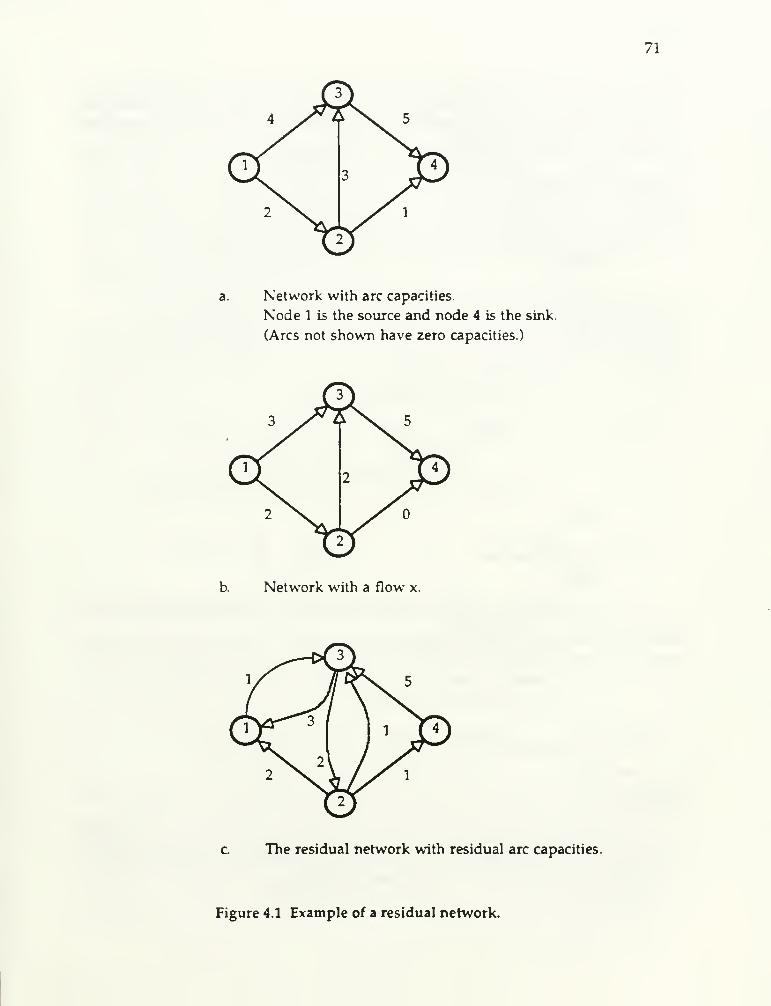
71

Network with arc capacities.

Node 1 is the source and node 4 is the sink.

(Arcs not shown have zero capacities.)

Network with a flow x.

c The residual network with residual arc capacities.

Figure 4.1 Example of a residua] network.

72

algorithm maintains a predecessor index, pred(i), for each labeled node i indicating the

rode that caused node i to be labeled. The predecessor indices allow us to trace back

along the path from a node to the source.

algorithm LABELING;

begin

loop

pred(j) : = for each j e N;

L: = (s);

while L * and t is unlabeled do

begin

select a node i € L;

for each (i, j) e A(i) do

if j is unlabeled and rj; > then

begin

pred(j) : = i;

mark j as labeled and add this node to L;

end

end;

if t is labeled then

begin

use the predecessor labels to trace back to obtain the augmenting path P

from s to t;

A : = min (rj; : (i, j) e P);

augment A units of flow along P;

erase all labels and go to loop;

end

else quit the loop;

end; (loop)

end;

The final residual capacities r can be used to obtain the arc flows as follows. Since

rjj = uj; - xj: + x:j,the arc flows satisfy xj: - x:j = uj; - Fjj. Hence, if u^: > rj: we can set x^; =

Ujj - r^; and x:j = 0; otherwise we set x^: = and x:j = fj; - u^;.

73

In order to show that the algorithm obtains a maximum flow, we introduce some

new definitions and notation. Recall from Section 1.3 that a set Q c A is a cutset if the

subnetwork G' = (N, A - Q) is disconnected eind no superset of Q Yias this property. A

cutset partitions set N into two subsets. A cutset is called am s-t cutset if the source and

the sink nodes are contained in different subsets of nodes S cind S = N - S: S is the set of

nodes connected to s. Conversely, any partition of the node set as S and S with s e S and

t e S defines an s-t cutset. Consequently, we alternatively designate an s-t cutset as

(S, S). An arc (i, j) with i e S cind j e S is called a forward arc, and an arc (i, j) with i e S

and j € S is called a backward arc in the cutset (S, S).

Let X be a flow vector satisfying the flow conservation and capacity constraints of

(4.1). For this flow vector X, let v be the amount of flow leaving the source. We refer

to v as the value of the flow. The flow x determines the net flow across an s-t cutset (S,

S) as

Fx<S< S)= X X_Xij - I_ X Xij. (4.2)

i G Sj e S i e S j e S

Def ne the capacity C(S, S) of an s-t cutset (S, S) is defined as

C(S, S) = X X "ij^'^•^^

ie S je S

We claim that the flow across any s-t cutset equals the value of the flow and does

not exceed the cutset capacity. Adding the flow conservation constraints (4.1 b) for nodes

in S and noting that when nodes i and j both belong to S, x^j in equation for nodej

Cemcels -Xjj in equation for node i, we obtain

^=1 I.'^ij - I_ X ''ij= Fx^S, S). (4.4)

ie S j€ S i€ S je S

Substituting x^; < u^; in the first summation and xj: ^ in the second summation

shows that

Fx(S, S)< X Z_ "ij ^ C<S, S). (4.5)

i€ S J6 S

74

This result is the weak duahty property of the maximum flow problem when

viewed as a linear program. Like most weak duality results, it is the "easy" half of the

duahty theory. The more substantive strong duaUty property cisserts that (4.5) holds as

an equality for some choice of x and some choice of an s-t cutset (S, S). This strong

duality property is the max-flow min-cut theorem.

Theorem 4.1. (Max-Flow Min-Cut Theorem) The maximum value of flow from s to I

equals the minimum capacity of all s-t cuts.

Proof. Let x denote the a maximum flow vector and v denote the maximum flow

value. (Linear programming theory, or our subsequent algorithmic developments,

guarantee that the problem always has a maximvmn flow as long eis some cutset has finite

capacity.) Define S to be the set of labeled nodes in the residual network G(x) when we

apply the labeling algorithm with the initial flow x. Let S = N - S. Clearly, since x is a

maximum flow, s e S and t e S. Adding the flow conservation equations for nodes in

S, we obtain (4.4). Note that nodes in S cannot be labeled from the nodes in S, hence rj:

= for each forward arc (i, j) in the cutset (S, S). Since rj: = U|; - Xj: + Xjj, the conditions

xjj < Ujj and x;, ^ imply that xj; = Uj; for each forward arc in the cutset (S, S) and x^; =

for each backward arc in the cutset. Making these substitutions in (4.4) yields

V = Fx(S, S) = ^ ]£ Ujj = C(S, S)

.

(4.6)

i e S j € S

But we have observed earlier that v is a lower bound on the capacity of any s-t cutset.

Coi^equently, the cutset (S, S) is a minimum capacity s-t cutset and its capacity equals

the maximum flow value v. We thus have established the theorem.

The proof of this theorem not only establishes the max-flow min-cut property,

but the same argument shows that when the labeling algorithm terminates, it has at

hemd both the maximum flow value (and a maximum flow vector) and a minimum

capacity s-t cutset. But does it terminate finitely? Each labeling iteration of the

algorithm scans any node at most once, inspecting each eirc in A(i). Consequently, the

labeling iteration scans each arc at most once <md requires 0(m) computations. If all arc

capacities are integral and bounded by a finite number U, then the capacity of the cutset

(s, N - {s}) is at most nU. Since the labeling algorithm increases the flow value by at least

one unit in any iteration, it terminates within nU iterations. This bound on the number

of iterations is not entirely satisfactory for large values of U; if U = 2", the bound is

75

exponential in the number of nodes. Moreover, the algorithm can indeed perform that

many iterations. In addition, if the capacities are irrational, the algorithm may not

terminate: although the successive flow values converge, they may not converge to the

maximum flow value. Thus if the method is to be effective, we must select the

augmenting paths carefully. Several refinements of the algorithms, including those we

consider in Section 4.2 - 4.4 overcome this difficulty and obtain an optimum flow even

if the capacities are irrational; moreover, the max-flow min-cut theorem (and our proof

of Theorem 4.1) is true even if the data are irrational.

A second drawback of the labeling algorithm is its "forgetfulness". At each

iteration, the algorithm generates node labels that contain information about

augmenting paths from the source to other nodes. The implementation we have

described erases the labels when it proceeds from one iteration to the next, even though

much of this information may be valid in the next residual network. Erasing the labels

therefore destroys potentially useful information. Ideally, we should retain a label when

it can be used profitably in later computations.

4.2 Decreasing the Number of Augmentations

The bound of nU on the number of augmentations in the labeling algorithm is

not satisfactory from a theoretical perspective. Furthermore, without further

modifications, the augmenting path algorithm may take fiCnU) augmentations, as the

example given in Figure 4.2 illustrates.

Flow decomposition shows that, in principle, augmenting path algorithms

should be able to find a maximum flow in no more thein m augmentations. For suppose

X is an optimum flow and y is any initial flow (possibly zero). By the flow decomposition

property, it is possible to obtain x from y by a sequence of at most m augmentations on

augmenting paths from s to t plus flows around augmenting cycles. If we define x' as

the flow vector obtained from y by applying only the augmenting paths, then x' also is a

maximum flow (flows around cycles do not change flow value). This result shows that

it is, in theory, possible to find a maximum flow using at most m augmentations.

Unfortunately, to apply this flow decomposition argument, we need to know a

maximum flow. No algorithm developed in the literature comes close to achieving this

theoretical bound. Nevertheless, it is possible to improve considerably on the bound of

0(nU) augmentations of the basic labeling algorithm.

76

10 \l

(a)

10^,0

(b)

10^,1

10^,1

(0

Figiire 4.2 A pathological example for the labeling algorithm.

(a) The input network with arc capacities.

(b) After aug^nenting along the path s-a-b-t. Arc flow is indicated beside the arc capacity.

(c) After augmenting along the path s-b-a-t. After 2 xlO^ augmentations, alternately

along s-a-b-t and s-b-a-t, the flow is maximum.

77

One natural specialization of the augmenting path algorithm is to augment flow

along a "shortest path" from the source to the sink, defined as a path consisting of the

least number of arcs. If we augment flow along a shortest path, then the length of any

shortest path either stays the same or increases. Moreover, within m augmentations, the

length of the shortest path is guaranteed to increase. (We will prove these results in the

next section.) Since no path contains more than n-1 arcs, this rule guarantees that the

number of augmentations is at most (n-l)m.

An alternative is to augment flow along a path of maximum residual capacity.

This specialization also leads to improved complexity. Let v be any flow value and v* be

the maximum flow value. By flow decomposition, the network contains at most maugmenting paths whose residual capacities sum to (v* - v). Thus the maximum

capacity augmenting path has residual capacity at least (v*-v)/m. Now consider a

sequence of 2m consecutive maximum capacity augmentations, starting with flow v. At

least one of these augmentations must augment the flow by an amount (v* - v)/2m or

less, for otherwise we will have a maximum flow. Thus after 2m or fewer

augmentations, the algorithm would reduce the capacity of a maximum capacity

augmenting path by a factor of at least two. Since this capacity is initially at most U and

the capacity must be at least 1 until the flow is maximum, after 0(m log U) maximum

capacity augmentations, the flow must be maximum. (Note that we are essentially

repeating the argument used to establish the geometric improvement approach

discussed in Section 1.6.)

In the following section, we consider another algorithm for reducing the number

of augmentations.

4.3 Shortest Augmenting Path Algorithm

A natural approach to augmenting along shortest paths would be to successively

look for shortest paths by performing a breadth first search in the residual network. If

the labeling algorithm maintains the set L of labeled nodes as a queue, then by

examining the labeled nodes in a first-in, first-out order, it would obtain a shortest path

in the residual network. Each of these iterations would take 0(m) steps both in the worst

case and in practice, and (by our subsequent observations) the resulting computation

time would be O(nm^). Unfortunately, this computation time is excessive. We can

improve this running time by exploiting the fact that the minimum distance from any

78

node i to the sink node t is monotonically nondecreasing over all augmentations. By

fully exploiting this property, we can reduce the average time per augmentation to 0(n).

The Algorithm

The concept of distance labels w^ill prove to be an important construct in the

maximum flow algorithms that we discuss in this section and in Sections 4.4 and 4.5. Adistance function d : N -* Z"*" with respect to the residual capacities Tj: is a fimction from

the set of nodes to the nonnegative integers. We say that a distance function is valid if it

satisfies the follovdng two conditions:

C4.1 d(t) = 0;

C4-2. d(i) < d(j) + 1 for every arc (i, j) € A with r^; > 0.

We refer to d(i) as the distance label of node i and condition C4.2 as the validit}/

condition. It is easy to demonstrate that d(i) is a lower boimd on the length of the

shortest directed path from i to t in the residual network. Let i = i^ - i2 - i3 - ... -\ - t

be any path of length k in the residual network from node i to t. Then, from C4.2 wehave d(i) = d(i|) < d(i2) + 1, d(i2) 2 d(i3) + 1, ... , d(ij^) < d(t) + 1 = 1. These inequalities

imply that d(i) < k for any path of length k in the residual network and, hence, any

shortest path from node i to t contains at leaist d(i) arcs. If for each node i, the distance

label d(i) equals the length of the shortest path from i to t in the residual network, then

we call the distance labels exact. For example, in Figure 4.1(c), d = (0, 0, 0, 0) is a valid

distance label, though d = (3, 1, 2, 0) represents the exact distance label.

We now define some additional notation. An arc (i, j) in the residual network is

admissible if it satisfies d(i) = d(j) + 1. Other arcs are inadmissible. A path from s to t

consisting entirely of admissible arcs is an admissible path. The algorithm we describe

next repeatedly augments flow along admissible paths. For any admissible path of length

k, d(s) = k. Since d(s) is a lower bound on the length of any path from the source to the

sink, the algorithm augments flows along shortest paths in the residual network. Thus,

we refer to the algorithm as the shortest augmenting path algorithm.

Whenever we augment along a path, each of the distance labels for nodes in the

path is exact. However, for other nodes in the network it is not necessary to maintain

exact distances; it suffices to have valid distances, which are lower bounds on the exact

distances. There is no particular urgency to compute these distances exactly. By allowing

the distance label of node i to be less than the distance from i to t, we maintain flexibility

in the algorithm, without incuring any significant cost.

79

We can compute the initial distance labels by performing a backward breadth first

search of the residual network, starting at the sink node. The algorithm generates an

admissible path by adding admissible circs, one at a time, as follows. It maintains a path

from the source node to some node i', called the current node, consisting entirely of

admissible arcs. We call this path a partial admissible path and store it using predecessor

indices, i.e., pred(j) = i for each arc (i, j) on the path. The algorithm performs one of the

two steps at the current node: advance or retreat. The advance step identifies some

admissible arc (i*, j*) emanating from node i*, adds it to the partial admissible path, and

designates j* as the new current node. If no admissible arc emanates from node i*, then

the algorithm performs the retreat step. This step increeises the distance label of node i*

so that at least one admissible arc emanates from it (we refer to this step as a relabel

operation). Increasing d(i*) makes the arc (predd*), i*) inadmissible (assuming i* # s).

Consequently, we delete (pred(i*), i*) from the partial admissible path and node pred(i*)

becomes the new current node. Whenever the partial admissible path becomes an

admissible path (i.e., contains node t), the algorithm makes a maximum possible

augmentation on this path and begins again with the source as the current node. The

algorithm terminates when d(s) S n, indicating that the network contains no

augmenting path from the source to the sink. We next describe the algorithm formally.

algorithm SHORTEST AUGMENTING PATH;

begin

X : = 0;

perform backward breadth first search of the residual network

from node t to obtain the distance labels d(i);

1* : = s;

while d(s) < n do

begin

if i* has an admissible arc then ADVANCE(i*)

else RETREAT(i*);

if i* = t then AUGMENT and set i» : = s;

end;

end;

procedure ADVANCE(i»);

begin

let (i*, j*) be an admissible arc in A(i*);

pred(j') : = i* and i* : = j*;

end;

80

procedure RETREAT(i');

begin

d(i*) : = min { d(j) + 1 : (i, j) € A(i*) and ^- > );

if !• ?t s then i* : = pred(i*);

end;

procedure AUGMENT;

begin

using predecessor indices identify an augmenting path P from the source to the

sink;

A : = min {rjj : (i, j) € P);

augment A units of flow along path P;

end;

We use the following data structure to select an admissible arc emanating from a

node. We maintain the list A(i) of arcs emanating from each node i. Arcs in each list

can be arranged arbitrarily, but the order, once decided, remains unchanged throughout

the algorithm. Each node i has a current-arc (i, j) which is the current candidate for the

next advance step. Initially, the current-arc of node i is the first arc in its arc list. The

algorithm examines this list sequentially and whenever the current arc is inadmissible,

it makes the next arc in the arc list the current arc. When the algorithm has examined

all arcs in A(i), it updates the distance label of node i and the current arc once again

becomes the first arc in its arc list. In our subsequent discussion we shall always

implicitly assume that the algorithms select admissible arcs using this technique.

Correctness of the Algorithm

We first show that the shortest augmentation algorithm correctly solves the

maximum flow problem.

Lemma 4.1. The shortest augmenting path algorithm maintains valid distance labels at

each step. Moreover, each relabel step strictly increases the distance label of a node.

Proof. We show that the algorithm maintains valid distance labels at every step by

performing induction on the number of augment and relabel steps. Initially, the

algorithm constructs valid distance labels. Assume, inductively, that the distance

function is valid prior to a step, i.e., satisfies the validity condition C4.2. We need to

check whether these conditions remain valid (i) after an augment step (when the

residual graph changes), and (ii) after a relabel step.

81

(i) A flow augmentation on arc (i, j) might delete this arc from the residual

network, but this modification to the residual network does not affect the validity of the

distance function for this arc. Augmentation on arc (i, j) might, however, create an

additional arc (j, i) with rjj > and, therefore, also create an additional condition d(j) <

d(i) + 1 that needs to be satisfied. The distance labels satisfy this validity condition,

though, since d(i) = d(j) + 1 by the admissibility property of the augmenting path.

(ii) The algorithm performs a relabel step at node i when the current arc reaches

the end of arc list A(i). Observe that if an arc (i, j) is inadmissible at some stage, then it

remains inadmissible until d(i) increases because of our inductive hypothesis that

distance labels are nondecreasing. Thus, when the current arc reaches the end of the arc

list A(i), then no arc (i, j) e A(i) satisfies d(i) = d(j) + 1 and rj; > 0. Hence, d(i) <

min{d(j) + 1 : (i, j) € A(i) and rj; > 0) = d'(i), thereby establishing the second part of the

lemma.

Finally, the choice for changing d(i) ensures that the condition d(i) < d(j) + 1

remains valid for all (i, j) in the residual network; in addition, since d(i) increases, the

conditions dOc) < d(i) + 1 remain valid for all arcs Gc, i) in the residual network.

Theorem 4.2. The shortest augmenting path algorithm correctly computes a maximumflow.

Proof. The algorithm terminates when d(s) ^ n. Since d(s) is a lower bound on the

length of the shortest augmenting path from s to t, this condition implies that the

network contains no augmenting path from the source to the sink, which is the

termination criterion for the generic augmenting path algorithm.

At termination of the algorithm, we can obtain a minimum s-t cutset as follows.

For < k < n, let a^ denote the number of nodes with distance label equal to k. Note

that Oj^, must be zero for some k* < n - 1 since V Oj^ ^n-1. (Recall that d(s) ^ n.)

- k =Let S = {i e N: d(i) > k*) and S = N - S. When d(s; ^ n and the algorithm terminates, s e

S and t e S, and both the sets S and S are nonempty. Consider the s-t cutset (S, S). By

construction, d(i) > d(j) + 1 for all (i, j) e (S, S). The validity condition C4.2 implies that

rj: = for each (i, j) e (S, S). Hence, (S, S) is a minimum s-t cutset and the current flow

is maximum.

82

Complexity of the Algorithm

We next show that the algorithm computes a maximvun flow in O(n^m) time.

Lemma 4.2. (a) Each distance label increases at most n times. Consequently, the total

number of relabel steps is at most n^ . (b) The number of augment steps is at most nrnfl.

Proof. Each relabel step at node i increeises d(i) by at least one. After the algorithm has

relabeled node i at most n times, d(i) S n. From this point on, the algorithm never

selects node i again during an advance step since for every node k in the current path,

d(k) < d(s) < n. Thus the algorithm relabels a node at most n times and the total number

of relabel steps is bounded by n'^.

Each augment step saturates at least one arc, i.e., decreases its residual capacity to

zero. Suppose that the arc (i, j) becomes saturated at some iteration (at which d(i) = d(j)

+ 1). Then no more flow can be sent on (i, j) until flow is sent back from j to i (at

which point d'(j) = d'(i) + 1 ^ d(i) + 1 = d(j) + 2). Hence, between two consecutive

saturations of arc (i, j) , d(j) increases by at least 2 units. Cortsequently, any arc (i, j) can

become saturated at most n/2 times and the total number of arc saturations is no more

than nm/2.

Theorem 4.3. The shortest augmenting path algorithm runs in O(n^m) time.

Proof. The algorithm performs 0(nm) flow augmentations and each augmentation takes

0(n) time, resulting in O(n^m) total effort in the augmentation steps. Each advance step

increases the length of the partial admissible path by one, and each retreat step decrecises

its length by one; since each partial admissible path has length at most n, the algorithm

requires at most 0(n^ + n^m) advance steps. The first term comes from the number of

retreat (relabel) steps, and the second term from the number of augmentations, which

are bounded by nm/2 by the previous lemma.

For each node i, the algorithm performs the relabel operation 0(n) times, each

execution requiring 0( I A(i) I ) time. The total time spent in all relabel operations is

V n I A(i) I = 0(nm). Finally, we consider the time spent in identifying admissible

i€ Narcs. The time taken to identify the admissible arc of node i is 0(1) plus the time sf)ent in

scanning arcs in A(i). After having performed I A(i) I such scannings, the algorithm

reaches the end of the arc list and relabels node i. Thus the total time spent in all

83

scannings is 0( V nlA(i)l) = 0(nm). The combination of these time bounds

i€ N

establishes the theorem.

The proof of Theorem 4.3 also suggests an alternative temnination condition for

the shortest augmenting path algorithm. The termination criteria of d(s) ^ n is

satisfactory for a worst-case analysis, but may not be efficient in practice. Researchers

have observed empirically that the algorithm spends too much time in relabeling, a

major portion of which is done after it has already found the maximum flow. The

algorithm can be improved by detecting the presence of a minimum cutset prior to

performing these relabeling operations. We can do so by maintaining the number of

nodes aj^ with distance label equal to k, for ^ k < n. The algorithm updates this array

after every relabel operation and terminates whenever it first finds a gap in the a array,»

i.e., ex. = for some k* < n. As we have seen earlier, if S = { i : d(s) > k*), then (S, S)

denotes a minimum cutset.

The idea of augmenting flows along shortest paths is intuitively appealing and

easy to implement in practice. The resulting algorithms identify at most 0(nm)

augmenting paths and this bound is tight, i.e., on particular examples these algorithms

perform f2(nm) augmentations. The only way to improve the running time of the

shortest augmenting path algorithm is to perform fewer computations per

augmentation. The use of a sophisticated data structure, called dynamic trees , reduces

the average time for each augmentation from 0(n) to OGog n). This implementation of

the maximum flow algorithm runs in 0(nm log n) time and obtaining further

improvements appears quite difficult except in very dense networks. These

implementations Vkith sophisticated data structures appear to be primarily of theoretical

interest, however, because maintaining the data structures requires substantial overhead

that tends to increase rather than reduce the computationjd times in practice. A detailed

discussion of dynamic trees is beyond the scope of this chapter.

Potential Functions and an Alternate Proof of Lemma 4.2(b)

A powerful method for proving computational time bounds is to use potential

functions. Potential function techniques are general purpose techniques for proving the

complexity of an algorithm by analyzing the effects of different steps on an appropriately

•defined function. The use of potential functions enables us to define an "accounting"

relationship between the occurrences of various steps of an algorithm that can be used to

84

obtain a bound on the steps that might be difficult to obtain using other arguments.

Rather than formally introducing potential functions, we illustrate the technique by

showing that the number of augmentations in the shortest augmenting path algorithm

is 0(nm).

Suppose in the shortest augmenting path algorithm we kept track of the number

of admissible arcs in the residual network. Let F(k) denote the number of admissible

arcs at the end of the k-th step; for the purpose of this argument, we count a step either eis

an augmentation or as a relabel operation. Let the algorithm perform K steps before it

terminates. Clearly, F(0) < m and F(K) ^ 0. Each augmentation decreases the residual

capacity of at least one arc to zero and hence reduces F by at least one unit. Each

relabeling of node i creates as many cis I A(i) I new admissible arcs, and increases F by the

same amount. This increase in F is at most nm over all relabelings, since the algorithm

relabels any node at most n times (as a consequence of Lemma 4.1) and V n I A(i) I =

i€ Nnm. Since the initial value of F is at most m more than its terminal value, the total

decrease in F due to all augmentations is m + nm. Thus the number of augmentations

is at most m + nm = 0(nm).

This argument is fairly representative of the potential function argument. Our

objective was to bound the number of augmentations. We did so by defining a potential

function that decreases whenever the algorithm performs an augmentation. The

potential increases only when the algorithm relabels distances, and thus we can bound

the number of augmentations using bounds on the number of relabels. In general, we

bound the number of steps of one type in terms of knovm boiands on the number of

steps of other types.

4.4 Freflow-Push Algorithms

Augmenting path algorithms send flow by augmenting along a path. This basic

step further decomposes into the more elementary operation of sending flow along an

arc. Thus sending a flow of A units along a path of k arcs decomposes into k basic

operations of sending a flow of A units along an arc of the path. We shall refer to each of

these basic operations as a push.

A path augmentation has one advantage over a single push: it maintains

conservation of flow at all nodes. In fact, the push-based algorithms such as those we

develop in this and the following sections necessarily violate conservation of flow.

85

Rather, these algorithms permit the flow into a node to exceed the flow out of this node.

We will refer to any such flows as preflows. The two basic operations of the generic

preflow-push methods are (i) pushing the flow on an admissible arc, and (ii) updating a

distance label, as in the augmenting path algorithm described in the last section. (We

define the distance labels and admissible arcs as in the previous section.)

Preflow-push algorithms have several advantages over augmentation based

algorithms. First, they are more general and more flexible. Second, they can push flow

closer to the sink before identifying augmenting paths. Third, they are better suited for

distributed or parallel computation. Fourth, the best preflow-push algorithms currently

outperform the best augmenting path algorithms in theory as well as in practice.

The Generic Algorithm

A preflow x is a function x: A —» R that satisfies (4.1c) and the following relaxation

of (4.1b):

y Xjj - y '^ijSO ,foralli€ N-{s, t).

{j:(j,i) € A) (j:(i,j) € A)

The preflow-push algorithms maintain a preflow at each intermediate stage. For

a given preflow x, we define the excess for each node i e N - {s, t} as

e(»>= Z ''ji - X'^ij•

{) : (j, i) € A) (j : (i, j) € A)

We refer to a node with positive excess as an active node. We adopt the

convention that the source and sink nodes are never active. The preflow-push

algorithms perform all operations using only local information. At each iteration of the

algorithm (except its initialization and its termination), the network contains at le<ist one

active node, i.e., a node i e N - {s, t) with e(i) > 0. The goal of each iterative step is to

choose some active node and to send its excess closer to the sink, closeness being

measured with respect to the current distance labels. As in the shortest aug;menting path

algorithms, we send flow only on admissible arcs. If the method cannot send excess

from this node to nodes with smaller distance labels, then it increases the distance label

of the node so that it creates at least one new admissible arc. The algorithm terminates

when the network contains no active nodes. The preflow-push algorithm uses the

following subroutines:

86

procedure PREPROCESS;

begin

x: = 0;

perform a backward breadth first-search of the residual network, stairting at node t,

to determine initial distance labels d(i);

Xgj : = Ugj for each arc (s, j) e A(s) and d(s) : = n;

end;

procedure PUSH/RELABEL(i);

begin

if the network contains an admissible arc (i, j) then

push 5 : = min{e(i), r^:) units of flow from node i to nodej

else replace d(i) by min {d(j) + 1 : (i, j) e A(i) and Tj: > 0};

end;

A push of 5 units from node i to node j decreases both e(i) and r^: by 6 units and

increases both e(j) and r;, by 5 units. We say that a push of 6 units of flow on arc (i, j) is

saturating if 5 = rj; and nonsaturating otherwise. We refer to the process of increasing

the distance label of a node as a relabel operation. The piirpose of the relabel operation is

to create at least one admissible arc on which the algorithm can perform further pushes.

The following generic version of the preflow-push algorithm combines the

subroutines just described.

algorithm PREFLOW-PUSH;

begin

PREPROCESS;

while the network contains an active node do

begin

select an active node i;

PUSH/RELABEL(i);

end;

end;

It might be instructive to visualize the generic preflow-push algorithm in terms

of a physical network; arcs represent flexible water pipes, nodes represent joints, and the

distance function measures how far nodes are above the ground; and in this network,

we v^h to send water from the source to the sink. In addition, we visualize flow in an

87

admissible arc as water flowing downhill. Initially, we move the source node upward,

and water flows to its neighbors. In general, water flows downhill towards the sink;

however, occasionally flow becomes trapped locally at a node that has no downhill

neighbors. At this point, we move the node upward, and again water flows downhill

towards the sink. Eventually, no flow than can reach the sink. As we continue to move

nodes upwards, the remaining excess flow eventually flows back towards the source.

The algorithm terminates when all the water flows either into the sink or into the

source.

Figure 4.3 illustrates the push/relabel steps applied to the example given in

Figure 4.1(a). Figure 4.3(a) specifies the preflow determined by the preprocess step.

Suppose the select step examines node 2. Since arc (2, 4) has residual capacity r24 = 1 and

d(2) = d(4) + 1, the algorithm performs a (saturating) push of value 6 = min {2, 1} units.

The push reduces the excess of node 2 to 1. Arc (2, 4) is deleted from the residual

network and arc (4, 2) is added to the residual network. Since node 2 is still an active

node, it can be selected again for further pushes. The arc (2, 3) and (2, 1) have positive

residual capacities, but they do not satisfy the distance condition. Hence, the algorithm

performs a relabel operation and gives node 2 a new distance d'(2) = min {d(3) + 1,

d(l)+l} = min{2,5) = 2.

The preprocessing step accomplishes several important tasks. First, it gives each

node adjacent to node s a positive excess, so that the algorithm can begin by selecting

some node with positive excess. Second, since the preprocessing step saturates all arcs

incident to node s, none of these arcs is admissible and setting d(s) = n will satisfy the

validity condition C4.2. Third, since d(s) = n is a lower bound on the length of any

shortest path from s to t, the residual network contains no path from s to t. Since

distances in d are nondecre<ising, we are also guaranteed that in subsequent iterations

the residual network will never contain a directed path from s to t, and so there never

will be any need to push flow from s again.

In the push/relabel(i) step, we identify an admissible arc in A(i) using the same

data structure we used in the shortest augmenting path algorithm. We maintain vrith

each node i a current arc (i, j) which is the current candidate for the push operation. Wechoose the current arc by sequentially scanning the arc list. We have seen earlier that

scanning the arc lists takes 0(nm) total time, if the algorithm relabels each node 0(n)

times.

88

d(3) = 1

e3=4

d(l) = 4 d(4) =

d(2) = 1

e,= 2

(a) The residual network after the preprocessing step.

d(3) = 1

d(l) = 4 d(4) =

d(2) = l

6^ = 1

(b) After the execution of step PUSH(2).

89

d(3) = 1

d(l) = 4 d(4) =

d(2) = 2

(c) After the execution of step RELABEL(2).

Figure 4.3 An illustration of push and relabel steps.

Assuming that the generic preflow-push algorithm terminates, we can easily

show that it finds a maximum flow. The algorithm terminates when the excess resides

either at the source or at the sink implying that the current preflow is a flow. Since d(s) =

r, the residual network contains no path from the source to the sink. This condition is

the termination criterion of the augmenting path algorithm, and thus the total flow on

arcs directed into the sink is the maximum flow value.

Complexity of the Algorithm

We now analyze the complexity of the algorithm. We begin by establishing one

important result: that distance labels are always valid and do not increase too many

times. The first of these conclusions follows from Lemma 4.1, because as in the shortest

augmenting path algorithm, the preflow-push algorithm pushes flow only on

admissible arcs and relabels a node orily when no admissible arc emanates from it. The

second conclusion follows from the following lemma.

Lemma 43. At any stage of the preflow-push algorithm, each node i with positive excess

is connected to node s by a directed path from i to s in the residual network.

Proof. By the flow decomposition theory, any preflow x can be decomposed with respect

to the original network G into nonnegative flows along (i) paths from the source s to t,

(ii) paths from s to active nodes, and (iii) the flows around directed cycles. Let i be an

90

active node relative to the preflou' x in G. Then there must be a path P from s to i in the

flow decomposition of x, since paths from s to t and flows around cycles do not

contribute to the excess at node i. Then the residual network contains the reversal of P

O' with the orientation of each arc reversed), and hence a directed path from i to s.

This lemma imples that during a relabel step, the algorithm does not minimize

over an empty set.

Lemma 4.4. For each node i e N, dii) < 2n.

Proof. The last time the algorithm relabeled node i, it had a positive excess, and hence

the residual network contained a path of length at most n-1 from node i to node s. The

fact that d(s) = n and condition C4.2 imply that d(i) < d(s) + n - 1 < 2n.

Lemma 4.5. (a) Each distance label increases at most 2n times. Consequently, the total

number of relabel steps is at most 2n^ . (b) The number of saturating pushes is at most

nm.

Proof. The proof is ver>' much similar to that of Lemma 4.2.

Lemma 4.6. The number of nonsaturating pushes is O(n^m).

Proof. We prove the lemma using an argument based on potential functions. Let I

denote the set of active nodes. Cor^ider the potential function F = V d(i). Since III <

. i€ I

n, and d(i) < 2n for all i e I, the initial value of F (after the preprocessing step) is at most

2n^. At termination, F is zero. During the push/relabel (i) step, one of the following two

cases must apply:

Case 1. The <ilgorithm is unable to find an admissible arc along which it can push flow.

In this case the distance label of node i increases by e ^ 1 units. This operation increases F

by at most e units. Since the total increase in d(i) throughout the running time of the

algorithm for each node i is bounded by 2n, the total increase in F due to increases in

distance labels is bounded by 2n''.

Case 2. The algorithm is able to identify an arc on which it can push flow, and so it

performs a saturating or a nonsaturating push. A saturating push on arc (i, j) might

create a new excess at node j, thereby increasing the number of active nodes by 1, and

increasing F by d(j), which may be as much as 2n per saturating push, and hence 2n'^m

over all saturating pushes. Next note that a nonsaturating push on arc (i, j) does not

91

increase III. The nonsaturatirg push will decrease F by d(i) since i becomes inactive,

but it simultaneously increases F by d(j) = d(i) - 1 if the push causes node j to become

active. If node j was active before the push, then F decrejises by an amount d(i). The net

decreeise in F is at least 1 unit per norxsaturating push.

We summarize these facts. The initial value of F is at most 2n^ and the

maximum possible increase in F is Irr- + 2n^m. Each nonsaturating push decreases F by

one unit and F always remains nonnegative. Hence, the nortsaturating pushes can occur

at most 2n^ + 2n^ + 2n^m = O(n^m) times, proving the lemma.

Finally, we indicate how the algorithm keeps track of active nodes for the

push/relabel steps. The algorithm maintains a set S of active nodes. It adds to S nodes

that become active following a push and are not already in S, and deletes from S nodes

that become inactive following a nonsaturating push. Several data structures (for

example, doubly linked lists) are available for storing S so that the algorithm can add,

delete, or select elements from it in 0(1) time. Consequently, it is easy to implement the

preflow-push algorithm in O(n'^m) time. We have thus established the following

theorem:

Theorem 1.4 The generic preflow-push algorithm runs in O(n'^m) time.

A Specialization of the Generic Algorithm

The running time of the generic preflow-push algorithm is comparable to the

bound of the shortest augmenting path algorithm. However, the preflow-push

algorithm has several nice features, in particular, its flexibility and its potential for

further improvements. By specifying different rules for selecting nodes for push/relabel

operations, we can derive many different algorithms from the generic version. For

example, suppose that we always select an active node with the highest distance label for

push/relabel step. Let h* = max {d(i) : e(i) > 0, i e N) at some point of the algorithm.

Then nodes with distance h* push flow to nodes with distance h*-l, and these nodes, in

turn, push flow to nodes with distance h*-2, and so on. If a node is relabeled then

excess moves up and then gradually comes dov^n. Note that if the algorithm relabels no

node during n cor\secutive node examinations, then all excess reaches the sink node and

the algorithm terminates. Since the algorithm requires O(n^) relabel operations, we

immediately obtain a bound of O(n^) on the number of node examinations. Each node

examination entails at most one nonsaturating push. Consequently, this algorithm

performs O(n^) nonsaturating pushes.

92

variable level which is an upper bound on the highest index r for which LlST(r) is

nonempty. We can store these lists as doubly linked lists so that adding, deleting, or

selecting an element takes 0(1) time. We identify the highest indexed nonempty list

starting at LIST(level) and sequentially scanning the lower indexed lists. We leave it as

an exercise to show that the overall effort needed to scan the lists is bounded by n plus

the total increase in the distance labels which is O(n^). The following theorem is now

evident.

Theorem 4.5 The preflcnv-push algorithm that always pushes flow from an active node ipith the

highest distance label runs in O(n^) time. U

The O(n^) bound for the highest label preflow push algorithm is straightforward,

and can be improved. Researchers have shown using more clever analysis that the

highest label preflow push algorithm in fact runs in 0(n^ Vrn ) time. We will next

describe another implementation of the generic preflow-push algorithm that

dramatically reduces the number of nonsaturating pushes, from O(n^m) to 0(n^ log U).

Recall that U represents the largest arc capacity in the network. We refer to this

algorithm as the excess-scaling algorithm since it is bcised on scaling the node excesses.

4.5 Excess-Scaling Algorithm

The generic preflow-push algorithm allows flows at each intermediate step to

violate mass balance equations. By pushing flows from active nodes, the algorithm

attempts to satisfy the meiss balance equations. The function ej^g^ ~ ^^'^ ^^^'^ : i is an

active node) is one measure of the infeasibility of a preflow. Note, though, that during

the execution of the generic algorithm, we would observe no particular pattern in Cj^^g^,

except that e^^g^^ eventually decreases to vtdue 0. In this section, we develop an excess-

scaling technique that systematically reduces Cjj^^ to 0.

The excess-scaling algorithm is based on the following ideas. Let A denote an

upper bound on ejj^g^ we refer to this bound as the excess-dominator . The excess-scaling

algorithm pushes flow from nodes whose excess is A/2 S ^jj^ax^^-"^^ choice assures

that during nonsaturating pushes the algorithm sends relatively large excess closer to the

sink. Pushes carrying small amounts of flow are of little benefit and can cause

bottlenecks that retards the algorithm's progress.

The algorithm also does not allow the maximum excess to increase beyond A.

This algorithmic strategy may prove to be useful for the following reason. Suppose

93

The algorithm also does not allow the maximum excess to increase beyond A.

This algorithmic strategy may prove to be useful for the following reason. Suppose

several nodes send flow to a single node j, creating a very large excess. It is likely that

node j could not send the accumulated flow closer to the sink, and thus the algorithm

Vkdll need to increase its distance and return much of its excess back toward the source.

Thus, pushing too much flow to any node is likely to be a wasted effort.

The excess-scaling algorithm has the follouang algorithmic description.

algorithm EXCESS-SCALING;

begin

PREPROCESS;

K:=2riogUl.

for k : = K down to do

begin (A-scaling phase)

A: = 2^

while the network contains a node i with e(i) > A/2 do

perform push/relabel(i) while ensuring that no node excess

exceeds A;

end;

end;

The algorithm performs a number of scaling phases with the value of the excess-

dominator A decreasing from phase to phase. We refer to a specific scaling phase with a

certain value of A as the /^-scaling phase. Initially, A = 2' ^°6 ^ ' when the logarithm has

base 2. Thus, U < A < 2U. Ehjring the A-scaling phase, A/2 < Cj^g^ < A and ejj^^^ may

vary up and down during the phase. When Cjj^g^ < A/2, a new scaling ph«ise begins.

After the algorithm has peformed flog Ul + 1 scaling phases, ejy,ax decreases to value

and we obtain the maximum flow.

The excess-scaling algorithm uses the same step push/relabel(i) as in the generic

preflow-push algorithm, but with one slight difference: instead of pushing 6 =

min {e(i), Tj;} units of flow, it pushes 6 = min {e(i), Ij;, A - e(j)} units. This change will

ensure that the algorithm permits no excess to exceed A. The algorithm uses the

following node selection rule to guarantee that no node excess exceeds A.

Selection Rule. Among all nodes with excess of more than A/2, select a node withminimum distance label (breaking ties arbitrarily).

94

Lemma 4.7. The algorithm satisfies the following two conditions:

C43. Each nonsaturating push sends at least A/2 units of flow.

C4.4. No excess ever exceeds A.

Proof. For every push on arc (i, j), we have e(i) > A/2 and e(j) < A/2, since node i is a

node with smallest distance label among nodes whose excess is more than A/2, and d(j)

= d(i) - 1 < d(i) since arc (i, j) is admissible. Hence, by sending min {e(i), r^;, A - e(j)) >

min {A/2, ijj) units of flow, we ensure that in a nonsaturating push the Jilgorithm sends

at leaist A/2 vmits of flow. Further, the push operation increases only e(j). Let e'(j) be the

excess at node j after the push. Then e'(j) = e(j) + min {e(i), Tj;, A - e(j)) <

e(j) + A - e(j) < A . All node excesses thus remain less than or equal to A.

Lemma 4.8. The excess-scaling algorithm performs O(n^) nonsaturating pushes per

scaling phase and 0(n^ log U) pushes in total.

Proof. Consider the potential function F = ^ e(i) d(i)/A. Using this potential function

ie N

we will establish the first assertion of the lemma. Since the algorithm has Odog U)

scaling phases, the second assertion is a consequence of the first. The initial value of F at

the beginning of the A-scaling phase is bounded by 2n^ because e(i) is bounded by A and

d(i) is bounded by 2n. During the push/relabeKi) step, one of the following two cases

must apply:

Case 1. The algorithm is unable to find an admissible arc along which it can push flow.

In this case the distance label of node i increases by e ^ 1 units. This relabeling operation

increases F by at most e units because e(i) < A. Since for each i, the totcil increaise in d(i)

throughout the running of the algorithm is bounded by 2n (by Lemma 4.4), the total

increase in F due to the relabeling of nodes is bounded by 2n^ in the A-scaling phase

(actually, the increase in F due to node relabelings is at most 2n'^ over all scaling phases).

Case 2. The algorithm is able to identify an arc on which it can push flow and so it

performs either a saturating or a nonsaturating push. In either Ccise, F decreases. A

nonsaturating push on arc (i, j) sends at leaist A/2 tmits of flow from node i to node j and

since d(j) = d(i) - 1, after this operation F decreaases by at least 1/2 units. Since the initial

value of F at the beginning of a A-scaling phase is at most 2n^ and the increases in F

during this scaling phase sum to at most 2n^ (from Case 1), the number of nonsaturating

pushes is bounded by 8rr.

95

This lemma implies a bound of 0(nm + n^ log U) for the excess-scaling

algorithm since we have already seen that all other operations — such as saturating

pushes, relabel operations and finding admissible arcs — require 0(nm) time. Up to this

point, we have ignored the method needed to identify a node with the minimum

distance label among nodes with excess more than A/2. Making this identification is

easy, if we use a scheme similar to the one used in the preflow-push method in Section

4.4 to find a node with the highest distance label. We maintain the lists LIST(r) = {i € N :

e(i) > A/2 and d(i) = r), and a variable level which is a lower bound on the smallest index

r for which LlST(r) is nonempty. We identify the lowest indexed nonempty list starting

at LIST(level) and sequentially scanning the higher indexed lists. We leave as an

exercise to show that the overall effort needed to scan the lists is bounded by the number

of pushes performed by the algorithm plus 0(n log U) and, hence, is not a bottleneck

operation. With this observation, we can summarize our discussion by the following

result.

Theorem 4.6 The preflow-push algorithm with excess-scaling runs in 0(nm + n^ log U)time.

Networks with Lower Bounds on Flows

To conclude this section, we show how to solve maximum flow problems vdth

nonnegative lower bounds on flows. Let /j; ^ denote the lower bound for flow on any

eu'C (i, j) e A. Although the maximum flow problem v^th zero lower bounds always

has a feasible solution, the problem wiih nonnegative lower bounds could be infecisible.

We can, however, determine the feeisibUlity of this problem by solving a maximum flow

problem with zero lower bounds as follows. We set x^: = /j: for each arc (i, j) e A. This

choice gives us a pseudoflow with e(i) representing the excess or deficit of any node i e

N. (We refer the reader to Section 5.4 for the definition of a pseudoflow with both

excesses and deficits). We introduce a super source, node s*, and a super sink, node t*.

For each node i with e(i) > 0, we add an arc (s*,i) with capacity e(i), and for each node i

with e(i) < 0, we add an arc (i, t*) with capacity -e(i). We then solve a maximum flow

problem from s* to t*. Let x* denote the maximum flow and v* denote the maximum

flow value in the transformed network. If v* = \ e(i) , then the original problem is

{i: e(i) > 0)

feasible and choosing the flow on each arc (i, j) as x^; + /jj is a feasible flow; otherwise,

the problem is infeasible.

96

Once we have found a feasible flow, we apply any of the maximum flow

algorithms with only one change: initially define the residual capacity of an arc (i, j) as

rj; = (ujj - Xjj) + (xjj - /jj). The first and second tenns in this expression denote,

respectively, the residual capacity for incre<ising flow on arc (i, j) cmd for decreasing flow

on arc (j, i). It is possible to establish the optimality of the solution generated by the

algorithm by generalizing the max-flow min-cut theorem to accomodate situations with

lower bounds. These observations show that it is possible to solve the maximum flow

problem with nonnegative lower bounds by two applications of the maximum flow

cilgorithms we have already discussed.

97

5. MINIMUM COST FLOWS

In this section, we consider algorithmic approaches for the minimum cost flow

problem. We consider the following node-arc formulation of the problem.

Minimize 2^ Cj; x;: {5.1a)

(i,j)€A^'

subject to

X X:: - X ''ii= t)(>)' for a" > e N, (5.1b)

{j : (i, j) € X) (j : (j, i) ^!k)

< xjj < Ujj, for each (i, j) € A. (5.1c)

We assume that the lower bounds /j; on arc flows are all zero and that arc costs are

nonnegative. Let C = max ( Cj; : (i, j) e A ) and U = max [ max { lb(i)l : ie N},

max ( ujj : (i, j) € A } ). The transformations Tl and T3 in Section 2.4 imply that these

assumptions do not impose any loss of generality. We remind the reader of our blanket

assumption that all data (cost, supply/demand and capacity) are integral. We also

assume that the minimum cost flow problem satisfies the following two conditions.

A5.1. Feasibility Assumption. We assume that X ^(^^ - and that the minimum cost

ieNflow problem has a feasible solution.

We can ascertain the feasibility of the minimum cost flow problem by solving a

maximum flow problem as follows. Introduce a super source node s*, and a super sink node

t*. For each node i with b(i) > 0, add an arc (s*, i) with capacity b(i), and for each node i

with b(i) < 0, add an arc (i, t*) with capacity -b(i). Now solve a maximum flow problem

from s* to t*. If the maximum flow value equals T b(i) then the minimum cost{i : b(D > 0)

flow problem is feasible; otherwise, it is infeasible.

A5.2. Connectedness Assumption. We assume that the network G contains an uncapacitated

directed path (i.e., each arc in the path has infinite capacity) between every pair of nodes.

We impose this condition, if necessary, by adding artificial arcs (1, j) and

(j, 1) for each j € N and assigning a large cost and a very large capacity to each of these

98

arcs. No such arc would appear in a minimum cost solution unless the problem

contains no feasible solution without artificial arcs.

CXir algorithms rely on the concept of residual networks. The residual network

G(x) corresponding to a flow x is defined as follows: We replace each arc (i, j) e A by two

arcs (i, j) and (j, i). The arc (i, j) has cost Cj: and residual capacity r^; = u^j - x^;, and the arc (j,

i) has cost -Cj: and residual capacity rjj = x^;. The residual network consists only of arcs

with positive residual capacity.

The concept of residual networks poses some notational difficulties. For

example, if the original network contains both the arcs (i, j) and (j, i), then the residual

network may contain two arcs from node i to node j and/or two arcs from node j to node

i with possibly different costs. Our notation for arcs assumes that at most one arc joins

one node to any other node. By using more complex notation, we can easily treat this

more general case. However, rather than changing our notation, we will tissume that

parallel arcs never arise (or, by inserting extra nodes on parallel arcs, we can produce a

network without any parallel arcs).

Observe that any directed cycle in the residual network G(x) is an augmenting

cycle with respect to the flow x and vice-versa (see Section 2.1 for the definition of

augmenting cycle). This equivalence implies the following alternate statement of

Theorem 2.4.

Theorem 5.1. A feasible flow x is an optimum flow if and only if the residual network G(x)

contains no negative cost directed cycle.

5.1. Duality and Optimality Conditions

As we have seen in Section 1.2, due to its special structure, the minimum cost

flow problem has a number of important theoretical properties. The linear

programming dual of this problem inherits many of these properties. Moreover, the

minimum cost flow problem and its dual have, from a linear programming point of

view, rather simple complementary slackness conditions. In this section, we formally

state the linear programming dual problem and derive the complementary slackness

conditions.

99

We consider the minimum cost flow problem (5.1) assuming that Uj; > for

each arc (i, j) € A. It is possible to show that this assumption imposes no loss of

generality. We associate a dual variable 7t(i) with the mass balance corwtraint of node i

in (5.1b). Since one of the constraints in (5.1b) is redundant, we can set one of these dual

variables to an arbitrary value. We, therefore , assume that 7c(l) = 0. Further, weassociate a dual variable 6jj with the upper bound constraint of arc (i, j) in (5.1c). The

dual problem to (5.1) is:

Maximize X t)(') '^(i^ ~ X "ij ^i\ (5 2a)ie N (i,j) e A ^ '

subject to

7c(i) - 7c(j) -6ij

< Cjj , for all (i, j) e A, (5.2b)

5jjS 0, foraU (i,j)e A, (5.2c)

and Ji(i) are unrestricted.

The complementary slackness conditions for this primal-dual pair are:

Xjj > => 7i(i) - n(j) - 5jj = Cjj

,

(5.3)

6jj > ^ Xjj = Ujj. (5.4)

These conditions are equivalent to the following optimality conditions:

Xj: = =* 7c(i) - 7t(j) < Cjj , (5.5)

0<xjj <u^j=* Jt(i)- Jt(j) = Cjj, (5.6)

Xij = Ujj=> n(i) - n{]) ^ qj

.

(5.7)

To see this equivalence, suppose that < Xj: < Uj: for some arc (i, j). The condition (5.3)

implies that

7t(i)-7t(j) -5jj = Cjj, (5.8)

Since Xj: < Uj; , (5.4) implies that 6jj = 0; substituting this result in (5.8) yields

(5.6). Whenever Xj; = Uj: > for some arc (i, j), (5.3) implies that n(i) - n(j) - 5jj = Cjj

.

100

Substituting 5jj S in this equation gives (5.7). Finally, if xj: = < uj; for some arc (i, j)

then (5.4) imples that 6jj = and substituting this result in (5.2b) gives (5.5).

We define the reduced cost of an arc (i, j) as Cj; = Cj: - Ji(i) + n(j). The conditions

(5.5) - (5.7) imply that a pair x, n of flows and node potentials is optimal if it satisfies

the follov^ing conditions:

C5.1 X is feasible.

C5.2 If Cjj > 0, then Xjj = 0.

C5.3 If Cjj = 0, then < Xj; < Ujj.

C5.4 If Cjj < 0, then x^: = U|j.

Observe that the condition C5.3 follows from the conditions C5.1, C5.2 and C5.4;

however, we retain it for the sake of completeness. These conditions, when stated in

terms of the residual network, simplify to:

C5.5 (Primal feasibility) x is feasible.

C5.6 (E>ual feasibility) Cj; t for each arc (i, j) in the residual network G(x).

Note that the condition C5.6 subsumes C5.2, C5.3, and C5.4. To see this result,

note that if Cj; > and Xj; > for some arc (i, j) in the original network, then the

residual network would contain arc (j, i) with Cjj = - Cjj. But then Cjj < 0, contradicting

C5.6. A similar contradiction arises if Cj; < and Xjj < Uj; for some (i, j) in A.

It is easy to establish the equivalence between these optimality conditions and the

condition stated in Theorem 5.1. Consider any pair x, n of flows and node potentials

satisf)'ing C5.5 and C5.6. Let W be any directed cycle in the residual network. Condition

C5.6 implies that X C:; S 0. Further , ^ S q: = X C;; + I (-Jt(i) + Jt(j))

(i,j)€ W '^(i,j)e W ''

(i,j)€ W (i,j)€ W

- -t^ Cjj . Hence, the residual network contains no negative cost cycle,

(i, i)eW

To see the converse, suppose that x is feasible and C(x) does not contain a

negative cycle. Then in the residual network the shortest distances from node 1, with

respect to the arc lengths Cj:, are well defined. Let d(i) denote the shortest distance from

node 1 to node i. The shortest path optimality condition C3.2 implies that d(j) < d(i) + q;

101

for aU (i, j) in G(x). Let n = - d. Then < q; + d(i) - d(j) = Cj; - Jt(i) + 7t(j) = Cj; for all (i, j)

in G(x). Hence, the pair x, 71 satisfies C5.5 and C5.6.

5^ Relationship to Shortest Path and Maximum Flow Problems

The minimum cost flow problem generalizes both the shortest path and

maximum flow problems. The shortest path problem from node s to all other nodes

can be formulated as a minimum cost flow problem by setting b(l) = (n - 1) , b(i) = -1 for

all 1 * s, and Uj; = «« for each (i, j) e A (in fact, setting Uj: equal to any integer greater

than (n - 1) will suffice if we wish to maintain finite capacities). Similarly, the

maximum flow problem from node s to node t can be transformed to the minimum cost

flow problem by introducing an additional arc (t, s) with c^g = -1 and u^^ = ~ (in fact, Uj^

= m • max {u|; : (i, j) e A) would suffice), and setting Cj: = for each arc (i, j) € A. Thus,

algorithms for the minimum cost flow problem solve both the shortest path and

maximum flow problems as special cases.

Conversely, algorithms for the shortest path and maximum flow problems are of

great use in solving the minimum cost flow problen.. Indeed, many of the algorithms

for the minimum cost flow problem either explicitly or implicitly use shortest path

and/or maximum flow algorithms as subroutines. Consequently, improved algorithms

for these two problems have led to improved algorithms for the minimum cost flow

problem. This relationship will be more transparent when we discuss algorithms for

the minimum cost flow problem. We have already shov^m in Section 5.1 how to obtain

an optimum dual solution from an optimum primal solution by solving a single

shortest path problem. We now show how to obtain an optimal primal solution from

an optimal dual solution by solving a single maximum flow problem.

Suppose that 7t is an optimal dual solution and c is the vector of reduced costs.

We define the cost-residual network G* = (N, A*) as follows. The nodes in G* have the

same supply/demand as the nodes in G. Any arc (i, j) e A* has an upper bound u^:* as

well as a lower bound 1^;*, defined as follows:

102

(i)

(ii)

For each (i, j) in A with Cj; > 0, A* contains an arc (i, j) with u^:* = 1j:» = 0.

For each (i, j) in A with Cj; < 0, A* contains an arc (i, j) with u^* = 1^:* =Uj;.

(iii) For each (i, j) in A with c,; = 0, A* contains an arc (i, j) with Uj;* = uj; and

hf = 0-

The lower and upper bounds on arcs in the cost-residual network G* are defined

so that any flow in G* satisfies the optimality conditions C5.2-C5.4. If Cj; > for some

(i, j) 6 A, then condition C5.2 dictates that xj: = in the optimum flow. Similarly, if

Cjj < for some (i, j) € A, then C5.4 implies the flow on arc (i, j) must be at the arc's

upper bound in the optimum flow. If cjj = 0, then any flow value will satisfy the

condition C5.3.

. r

Now the problem is reduced to finding a feasible flow in the cost-residual

network that satisfies the lower and upper bound restrictions of arcs and, at the same

time, meets the supply/demand constraints of the nodes. We first eliminate the lower

bounds of arcs as described in Section 2.4 and then transform this problem to a

maximum flow problem as described in assumption A5.1. Let x* denote the maximum

flow in the transformed network. Then x*+/* is an optimum solution of the minimum

cost problem in G.

5.3. Negative Cycle Algorithm

Operations researchers, computer scientists, electrical engineers and many others

have extensively studied the minimum cost flow problem and have proposed a number

of different algorithms to solve this problem. Notable examples are the negative cycle,

successive shortest path, primal-dual, out-of-kilter, primal simplex and scaling-based

algorithms. In this and the following sections, we discuss most of these important

algorithms for the minimum cost flow problem and point out relationships between

them. We first consider the negative cycle algorithm.

The negative cycle algorithm maintains a primal feasible solution x and strives

to attain dual feasibility. It does so by identifying negative cost directed cycles in the

residual network G(x) and augmenting flows in these cycles. The algorithm terminates

when the residual network contains no negative cost cycles. Theorem 5.1 implies that

when the algorithm terminates, it has found a minimum cost flow.

103

algorithm NEGATIVE CYCLE;

begin

establish a feasible flow x in the network;

while C(x) contains a negative cycle do

begin

use some algorithm to identify a negative cycle W;

5 : = min [t^ (i, j) e W);

augment 6 units of flow along the cycle W and update G(x);

end;

end;

A feasible flow in the network can be found by solving a maximum flow problem

as explained just after assumption A5.1. One algorithm for identifying a negative cost

cycle is the label correcting algorithm for the shortest path problem, described in Section

3.4, which requires 0(nm) time to identify a negative cycle. Every iteration reduces the

flow cost by at least one unit. Since mCU is an upper bound on an initial flow cost and

zero is a lower bound on the optimum flow cost, the algorithm terminates after at most

O(mCU) iterations and requires O(nm^CU) time in total.

This algorithm can be improved in the following three ways (which we briefly

irizpVsummarize)

(i) Identifying a negative cost cycle in effort much less than 0(nm) time. The simplex

algorithm (to be discussed later) nearly achieves this objective. It maintains a tree

solution and node potentials that enable it to identify a negative cost cycle in 0(m) effort.

However, due to degeneracy, the simplex algorithm cannot necessarily send a positive

amoimt of flow along this cycle.

(ii) Identifying a negative cost cycle with maximum improvement in the objective

function value. The improvement in the objective function due to the augmentation

- Ialong a cycle W is

(i, j) € W ^

(min (rjj : (i, j) e W)). Let x be some flow and x* be an

optimum flow. The augmenting cycle theorem (Theorem 2.3) implies that x* equals x

plus the flow on at most m augmenting cycles with respect to x. Further, improvements

in cost due to flow augmentations on these augmenting cycles sum to ex -ex*.

Consequently, at least one augmenting cycle with respect to x must decrease the objective

function by at least (ex -cx*)/m. Hence, if the algorithm always augments flow along a

104

cycle with maximum improvement, then Lemma 1.1 implies that the method would

obtain an optimum flow within 0(m log mCU) iterations. Finding a maximum

improvement cycle is a difficult problem, but a modest variation of this approach yields

a polynomial time algorithm for the minimum cost flow problem.

(iii) Identifying a negative cost cycle vdth minimum mean cost. We define the mean cost

of a cycle ais its cost divided by the number of arcs it contains. A minimum mean cycle is a

cycle whose mean cost is as small as possible. It is possible to identify a minimum mean

cycle in 0(nm) or 0(Vri m log nC) time. Recently, researchers have shown that if the

negative cycle algorithm always augments the flow along a minimum mean cycle, then

from one iteration to the next, the minimum mean cycle value is nondecreasing;

moreover, its absolute value decreases by a factor of l-(l/n) within m iterations. Since

the mean cost of the minimum mean (negative) cycle is bounded from below by -C and

bounded from above by -1/n, Lemma 1.1 implies that this algorithm will terminate in

0(nm log nC) iterations.

5.4. Successive Shortest Path Algorithm

The negative cycle algorithm maintains primal feasibility of the solution at every

step and attempts to achieve dual feaisibility. In contrast, the successive shortest path

algorithm maintains dual feasibility of the solution at every step and strives to attain

primal feasibility. It maintains a solution x that satisfies the normegativity and capacity

constraints, but violates the supply/demand constraints of the nodes. At each step, the

algorithm selects a node i with extra supply and a node j with unfulfilled demand and

sends flow from i to j along a shortest path in the residual network. The algorithm

terminates when the current solution satisfies all the supply/demand constraints.

A pseudoflow is a function x : A -» R satisfying only the capacity <md normegativity

constraints. For any pseudoflow x, we define the imbalance of node i as

e(i) = b(i) + X ''ii- X ''ii'

for all i e N.

{j: (j, i) € A] {j: (i,j) € a1

If e(i) > for some node i, then e(i) is called the excess of node i, if e(i) < 0, then

-e(i) is called the deficit. A node i vdth e(i) = is called balanced. Let S and T denote the

105

sets of excess and deficit nodes respectively. The residual network corresponding to a

pseudoflow is defined in the same way that we define the residual network for a flow.

The successive shortest path algorithm successively augments flow along shortest

paths computed with respect to the reduced costs Cj;. Observe that for any directed path

P from a node k to a node /, Z C;; = Y C:; - nil) + n(k). Hence, the node(i, fe P ''

(i, fe ?'>

potentials change all path lengths between a specific pair of nodes by a constant amount,

and the shortest path with respect to Cj; is the same bls the shortest path with respect to

Cjj. The correctness of the successive shortest path algorithm rests on the following

result.

Lemma 5.1. Suppose a pseudoflow x satisfies the dual feasibility condition C5.6 unth respect to the

node potentials it. Furthermore, suppose that x' is obtained from x by sending flow along a

shortest path from a node k to a node I in Gix). Then x' also satisfies the dual feasibility

conditions with respect to some node potentials.

Proof. Since x satisfies the dual feasibility conditions with respect to the node potentials

jt, we have Cj: ^ for all (i, j) in G(x). Let d(v) denote the shortest path distances from

node k to any node v in G(x) with respect to the arc lengths Cj;. We claim that x also

satisfies the dual feasibility conditions with re;pect to the potentials Jt' = 7t-d. The

shortest path optimality conditions (i.e., C3.2) imply that

d(j)<d(i)+ cjj , for all (i, j) in G(x).

Substituting Cj: = Cj; - Jt(i) + n(j) in these conditions and using 7t'(i) = 7t(i) - d(i) yields

qj" = Cjj - 7:'(i) + n'(j) S 0, for all (i, j) in G(x).

Hence, x satisfies C5.6 with respect to the node potentials n'. Next note that Cj;' = for

every arc (i, j) on the shortest path P from node k to node /, since d(j) = d(i) + Cjj for

every arc (i, j) € P and Cj: = c^; - ;c(i) + Jt(j).

We are now in a position to prove the lemma. Augmenting flow along any arc

in P maiintains the dual feasibility condition C5.6 for this arc. Augmenting flow on an

arc (i, j) may add its reversal (j, i) to the residual network. But since Cj: = for each arc

(i, j) 6 P , Cjj = 0, and so arc (j, i) also satisfies C5.6.

The node potentials play a very important role in this algorithm. Besides using

them to prove the correctness of the algorithm, we use them to ensure that the arc

106

lengths are nonnegative, thus enabling us to solve the shortest path subproblems more

efficiently. The following formal statement of the successive shortest path algorithm

summarizes the steps of this method.

algorithm SUCCESSIVE SHORTEST PATH;

begin

X : = and 7t : = 0;

compute imbalances e(i) and initialize the sets S and T;

while S ^ do

begin

select a node k e S and a node / € T;

determine shortest path distances d(j) from node k to all

other nodes in G(x) with respect to the reduced costs Cj;;

let P denote a shortest path from k to 1;

ujxJaten : = 7t-d;

6 : = min [ e(k), -e(/), min { rj: : (i, j) € P } ];

augment 6 units of flow along the path P;

update X, S and T;

end;

end;

To initialize the algorithm, we set x = 0, which is a feasible pseudoflow and

satisfies C5.6 with respect to the node potentials n = since, by assumption, all arc

lengths are nonnegative. Also, if 5*0, then T * because the sum of excesses always

equals the sum of deficits. Further, the connectedness assumption implies that the

residual network G(x) contains a directed path from node k to node /. Each iteration of

this algorithm solves a shortest path problem with nonnegative arc lengths and reduces

the supply of some node by at least one unit. Consequently, if U is an upper bound on

the largest supply of any node, the algorithm terminates in at most nU iterations. Since

the arc lengths Cj: are nonnegative, the shortest path problem at each iteration can be

solved using Dijkstra's algorithm. So the overall complexity of this algorithm is

0(nU S(n, m, O), where S(n, m, C) is the time taken by Dijkstra's algorithm. Currently,

the best strongly polynomial -time bound to implement Dijkstra's algorithm is CXm + n

log n) and the best (weakly) polynomial time bound is 0(min {m log log C, m +

nVlogC ) ). The successive shortest path algorithm is pseudopolynomial time since it is

polynomial in n, m and the largest supply U. The algorithm is, however, f>olynomial

107

time for the assignment problem, a special case of the minimum cost flow problem for

which U = 1. In Section 5.7, we will develop a polynomial time algorithm for the

minimum cost flow problem using the successive shortest path algorithm in

conjunction with scaling.

5.5. Primal-Dual and Out-of-Kilter Algorithms

The primal-dual algorithm is very similar to the successive shortest path problem,

except that instead of sending flow on only one path during an iteration, it might send

flow along many paths. To explain the primal-dual algorithm, we transform the

minimum cost flow problem into a single-source and single-sink problem (possibly by

adding nodes and arcs as in the assumption A5.1). At every iteration, the primal-dual

algorithm solves a shortest path problem from the source to update the node potentials

(i.e., as before, each 7:(j) becomes 7t(j) - d(j)) and then solves a maximum flow problem to

send the maximum possible flow from the source to the sink using only arcs with zero

reduced cost. The algorithm guarantees that the excess of some node strictly decreases at

each iteration, and also assures that the node potential of the sink strictly decreases. The

latter observation follows from the fact that after we have solved the maximum flow

problem, the network contains no path from the source to the sink in the residual

network consisting entirely of arcs with zero reduced costs; coi^equently, in the next

iteration d(t) ^ 1. These observations give a bound of min {nU, nC} on the number of

iterations since the magnitude of each node potential is bounded by nC. This bound is

better than that of the successive shortest path algorithm, but, of course, the algorithm

incurs the additional expense of solving a maximum flow problem at each iteration.

Thus, the algorithm has an overall complexity of 0(min (nU S(n, m, C), nC M(n, m, U)),

where S(n, m, C) and M(n, m, U) respectively denote the solution times of shortest p>ath

and maximum flow algorithms.

The successive shortest path and primal-dual algorithnw maintain a solution

that satisfies the dual feasibility conditions and the flow bound constraints, but that

violates the mass balance constraints. These algorithnns iteratively modify the flow and

potentials so that the flow at each step comes closer to satisfying the mass balance

constraints. However, we could just as well have violated other constraints at

intermediate steps. The out-of-kilter algorithm satisfies only the mass balance cortstraints

and may violate the dual feasibility conditions and the flow bound restrictior«. The basic

idea is to drive the flow on an arc (i, j) to Uj; if Cj: < 0, drive the flow to zero if Cj; > 0,

and to permit any flow between and Uj: if Cj: = 0. The kilter number, represented by k^:.

108

kjj, of an arc (i, j) is defined cis the minimum increase or decrease in the flow necessary to

satisfy its flow bound constraint and dual feasibility condition. For example, for an arc (i,

j) with Cjj > 0, k^j = I x^j I and for an arc (i, j) with c^j < 0, k^; = I u^; - x^: I . An arc with k^:

= is said to be in-kilter. At each iteration, the out-of-kilter algorithm reduces the kilter

number of at least one arc; it terminates when all arcs are in-kilter. Suppose the kilter

number of an arc (i, j) would decrease by increasing flow on the arc. Then the algorithm

would obtain a shortest path P from node j to node i in the residual network and

augment at least one unit of flow in the cycle P u {(i, j)). The proof of the correctness of

this algorithm is similar to, but more detailed than, that of the successive shortest path

algorithm.

5.6. Network Simplex Algorithm

The network simplex algorithm for the minimum cost flow problem is a

specialization of the bounded variable primal simplex algorithm for linear

programming. The special structure of the minimum cost flow problem offers several

benefits, particularly, streamlining of the simplex computations and eliminating the

»need to explicitly maintain the simplex tableau. The tree structure of the basis (see

Section 2.3) permits the algorithm to achieve these efficiencies. The advances made in

the last two decades for maintaining and upxiating the tree structure efficiently have

substantially improved the speed of the algorithm. Through extensive empirical testing,

researchers have also improved the performance of the simplex algorithm by

developing various heuristic rules for identifying entering variables. Though no

version of the primal network simplex algorithm is known to run in polynomial time,

its best implementations are empirically comparable to or better than other minimum

cost flow algorithms.

In this section, we describe the network simplex algorithm in detail. We first

define the concept of a basis structure and describe a data structure to store and to

manipulate the basis, which is a spanning tree. We then show how to compute arc flows

and node potentials for any basis structure. We next discuss how to perform various

simplex operations such as the selection of entering arcs, leaving arcs and pivots using

the tree data structiire. Finally, we show how to guarantee the finiteness of the network

simplex algorithm.

109

The network simplex algorithm maintains a basic feasible solution at each stage

A basic solution of the minimum cost flow problem is defined by a triple (B, L, U); B, L

and U p>artition the arc set A. The set B denotes the set of basic arcs, i.e., arcs of a spanrung

tree, and L and U respectively denote the sets of nonbasic arcs at their lower and upper

bounds. We refer to the triple (B, L, U) as a basis structure. A basis structure (B, L, U) is

called feasible if by setting Xj; = for each (i, j) e L, and setting xj: = u^: for each (i, j) g U,

the problem has a feasible solution satisfying (5.1b) and (5.1c). A feasible basis structure

(B, L, U) is called an optimum basis structure if it is possible to obtain a set of node

potentials n so that the reduced costs defined by Cj; = Cj; - nii) + n(j) satisfy the following

optimality conditions:

Cjj = , for each (i, j) e B, (5.9)

Cij S , for each (i, j) € L, (5.10)

Cjj < , for each (i, j) € U. , (5.11)

/

These optimality conditions have a nice economic interpretation. We shall see a

little later that if nil) = 0, then equations (5.9) imply that -7t(j) denotes the length of the

tree path in B from node 1 to node j. Then, cj; = Cj; - jc(i) + 7t(j) for a nonbeisic arc (i, p in

L denotes the change in the cost of flow achieved by sending one unit of flow through

the tree path from node 1 to node i, through the arc (i, j), and then returning the flow

along the tree path from node j to node 1. The condition (5.10) implies that this

circulation of flow is not profitable for any nonbasic arc in L. The condition (5.11) has a

similar interpretation.

The network simplex algorithm maintains a feasible basis structure at each

iteration and successively improves the basis structure until it becomes an optimum

basic structure. The following algorithmic description specifies the essential steps of the

procedure.

110

algorithm NETWORK SIMPLEX;

begin

determine an initial btisic feasible flow x and the corresponding

basis structure (B, L, U);

compute node potentials for this basis structure;

while some arc violates the optimality conditions do

begin

select an entering arc (k, /) violating the optimality conditions;

add arc (k, /) to the spanning tree corresponding to the baisis forming a cycle

and augment the maximum possible flow in this cycle;

determine the leaving arc (p, q);

perform a basis exchange and update node potentials;

end;

end;

In the following discussion, we describe the various steps performed by the

network simplex algorithm in greater detail.

Obtaining an Initial Basis Structure

Our connectedness assumption A5.2 provides one way of obtaining an initial

basic feasible solution. We have assumed that for every node j € N - {!), the network

contains arcs (1, j) and (j, 1) with sufficiently large costs and capacities. The initial basis B

includes the arc (1, j) with flow -b(j) if b(j) S and arc (j, 1) with flow b(j) if b(j) > 0. The

set L consists of the remaining arcs, jmd the set U is empty. The node potentials for this

basis are easily computed using (5.9), as we will see later.

Maintaining the Tree Structure

The specialized network simplex algorithm is possible because of the spanning

tree property of the beisis. The algorithm requires the tree to be represented so that the

simplex algorithm can perform operations efficiently and update the representation

quickly when the basis changes. We next describe one such tree representation.

We consider the tree as "hanging" from a specially designated node, called the

root. We assume that node 1 is the root node. See Figxire 5.1 for an example of the tree.

We associate three indices with each node i in the tree: a predecessor index, pred(i); a depth

index, depthd); and a thread index, thread(i). Each node i has a unique path connecting it

Ill

to the root. The predecessor index stores the first node in that path (other than node i)

and the depth index stores the number of arcs in the path. For the root node these

indices are zero. The Figure 5.1 shows an example of these indices. Note that by

iteratively using the predecessor indices, we can enumerate the path from any node to

the root node. We say that pred(i) is the predecessor of node i and i is a successor of node

pred(i). The descendants of a node i consist of the node i itself, its successors, successors of

its successors, and so on. For example, the node set (5, 6, 7, 8, 9) contair« the descendents

of node 5 in Figure 5.1. A node with no successors is called a leaf node. In Figure 5.1,

nodes 4, 7, 8, and 9 are leaf nodes.

The thread indices define a traversal of the tree, a sequence of nodes that walks or

threads its way through the nodes of the tree, starting at the root and visiting nodes in a

"top to bottom" and "left to right" order, and then finally returning to the root. The

thread indices can be formed by performing a depth first search of the tree as described in

Section 1.5 and setting the thread of a node to be the node encountered after the node

itself in this depth first search. For our example, this sequence would read

1-2-5-6-8-9-7-3-4-1 (see the dotted lines in Figure 5.1). For each node i, thread (i) specifies

the next node in the traversal visited after node i. This traversal satisfies the following

two properties; (i) the predecessor of each node appears in the sequence before the node

itself; and (ii) the descendants of any node are consecutive elements in the traversal.

The thread indices provide a particularly convenient means for visiting (or finding) all

descendants of a node i: We simply follow the thread from node i, recording the nodes

visited until the depth of the visited node becomes at least as large as node i. For

example, starting at node 5, we visit nodes 6, 8, 9, and 7 in order, which are the

descendants of node 5, and then visit node 3. Since node 3's depth equals that of node 5,

we know that we have left the "descendant tree" lying below node 5. As we will see,

finding the descendant tree of a node efficiently adds sigiuficantly to the efficiency of the

simplex method.

The simplex method has two basic steps: (i) determining the node p>otentials of a

given basis structure; and (ii) computing the arc flows for a given basis structure. Wenow describe how to perform these steps efficiently using the tree indices.

Computing Node Potentials and Flows for a Given Basis Structure

We first consider the problem of computing node potentials n for a given basis

structure (B, L, U). We assume that n(l) = 0. Note that the value of one node potential

112

can be set arbitrarily since one constraint in (5.1b) is redundant. We compute the

remaining node potentials using the conditions that Cj: = for each arc (i, j) in B. These

conditions can alternatively be stated as

1

113

n(j) = Ji(i) - Cjj, for every arc (i, j) e B. (5.12)

The basic idea is to start at node 1 and fan out along the tree arcs using the thread

indices to compute other node potentials. The traversal assures that whenever this

fanning out procedure visits node j, it has already evaluated the potential of its

predecessor, say node i; hence, the procedure can comput 7t(j) using (5.12). The thread

indices allow us to compute all node potentials in 0(n) time using the following

method.

procedure COMPUTE POTENTIALS;

begin

7t(l): = 0;

j: = thread(l);

while j ^ 1 do

begin

i : = pred(j);

if (i, j) 6 A then ;:(]) : = 7t(i) - Cj;;

if (j, i) € A then 7t(j) : = 7t(i) + Cjj;

j : = thread (j);

end;

end;

A similar procedure will permit us to compute flows on basic arcs for a given

basis structure (B, L, U). We proceed, however, in the reverse order: start at the leaf

node and move in toward the root using the predecessor indices, while computing flows

on arcs encountered along the way. The following procedure accomplishes this task.

114

procedure COMPUTE FLOWS;

begin

e(i) : = b(i) for aU i € N;

let T be the basis tree;

for each (i, j) e U do

set X|j : = u^j, subtract Uj; from e(i) and add u^: to e(j);

while T*{1) do

begin

select a leaf node j in the subtree T;

i : = pred(j);

if (i, j) € T then Xj; : = -e(j);

else Xjj : = e(j);

add e(j) to e(i);

delete node j and the arc incident to it from T;

end;

end;

One way of identifying leaf nodes in T is to select nodes in the reverse order of the

thread indices. A simple procedure completes this task in 0(n) time: push all the nodes

into a stack in order of their appearance on the thread, and then take them out from the

top one at a time. Note that in the thread traversal, each node appears prior to its

descendants. Hence, the reverse thread traversal examines each node after examining its

descendants.

Now consider the steps of the method. The arcs in the set U must carry flow

equal to their capacity. Thus, we set x^; = U|j for these arcs. This assignment creates an

additional demand of Uj; units at node i and makes the same amount available at node j.

This effect of setting Xj: = u^: explains the initial adjustments in the supply/demand of

nodes. The manner for up>dating e(j) implies that each e(j) represents the sum of the

adjusted supply/demand of nodes in the subtree hanging from node j. Since this subtree

is connected to the rest of the tree only by the arc (i, j) (or (j, i)), this arc must carry -e(j) (or

e(j)) units of flow to satisfy the adjusted supply/demand of nodes in the subtree.

The procedure Compute Flows essentially solves the system of equations Bx = b,

in which B represents the columns in the node-arc incidence matrix N corresponding to

the spanning tree T. Since B is a lower triangular matrix (see Theorem 2.6 in Section

2.3), it is possible to solve these equations by forward substitution, which is precisely

115

what the algorithm does. Similarly, the procedure Compute Potentials solves the system

of equations n B = c by back substitution.

Entering Arc

Two types of arcs are eligible to enter the basis: aiiy nonbasic arc at its lower

bound with a negative reduced cost or any nonbasic arc at its upper bound with a

positive reduced cost, is eligible to enter the basis. These arcs violate condition (5.10) or

(5.11). The method used for selecting an entering arc among these eligible arcs has a

inajor effect on the performance of the simplex algorithm. An implementation that

selects an arc that violates the optimality condition the most, i.e., has the largest value of

I Cjj I among such arcs, might require the fewest number of iterations in practice, but

must examine each arc at each iteration, which is very time<onsuming. On the other

hand, examining the arc list cyclically and selecting the first arc that violates the

optimality condition would quickly find the entering arc, but might require a relatively

large number of iterations due to the poor arc choice. One of the most successful

implementations uses a candidate list approach that strikes an effective compromise

between these two strategies. This approach also offers sufficient flexibility for fine

tuning to special problem classes.

The algorithm maintains a candidate list of arcs violating the optimality

conditions, selecting arcs in a two-phase procedure cor«isting of major iterations and

minor iterations. In a major iteration, we construct the candidate list. We examine arcs

emanating from nodes, one node at a time, adding to the candidate list the arcs

emanating from node i (if any) that violate the optimality condition. We repeat this

selection process for nodes i+1, i+2, ... until either we have examined all nodes or the list

has reached its maximum allowable size. The next major iteration begins with the node

where the previous major iteration ended. In other words, the algorithm examines

nodes cyclically as it adds arcs emanating from them to the candidate list.

Once the algorithm has formed the candidate list in a major iteration, it performs

minor iterations, scanning all candidate arcs and choosing a nonbasic arc from this list

that violates the optimality condition the most to enter the basis. As we scan the arcs,

we ufxiate the candidate list by removing those arcs that no longer violate the optimality

conditions. Once the list becomes empty or we have reached a specified limit on the

number of minor iterations to be performed at each major iteration, we rebuild the list

with another major iteration.

116

Leaving Arc^

Suppose we select the arc (k, 1) as the entering arc. The addition of this arc to the

basis B forms exactly one (undirected) cycle W, which is sometimes referred to as the

pivot cycle. We define the orientation of W as the same as that of (k, /) if (k, /) € L, and

opposite to the orientation of (k, /) if Oc, /) e U. Let W and W , respectively, denote the

sets of arcs in W along and opposite to the cycle's orientation. Sending additional flow

around the pivot cycle W in the direction of its orientation strictly decreases the cost of

the current solution. We change the flow as much as possible until one of the arcs in the

cycle W reaches its lower or upper bound; this arc leaves the basis. The maximum flow

change 5j: on an arc (i, j) e W that satisfies the flow bound constraints is

|Uj: - X|: , if (i, j) e W,

^j=[Xi;, if(i,j)eW.

We send 6 = min {5jj : (i, j) e W) units of flow around W, and select an arc (p, q)

with 5pQ = 6 as the leaving arc. The crucial operation in this step is to identify the cycle

W. If P(i) denotes the unique path in the basis from any node i to the root node, then

this cycle consists of the arcs {(((k, /)} u P(k) u P(/)) - (P(k) n P(/))). In other words, Wconsists of the arc (k, /) and the disjoint portions of P(k) and P(/). Using predecessor

indices alone permits us to identify the cycle W as follows. Start at node k and using

predecessor indices trace the path from this node to the root and label all the nodes in

this path. Repeat the same operation for node / until we encounter a node already

labeled, say node w. Node w, which we might refer to as the apex, is the first common

ancestor of nodes k and /. The cycle W contains the portions of the path P(k) and P(/) up

to node w, along with the arc (k, /). This method is efficient, but it can be improved. It

has the drawback of backtracking along some arcs that are not in W, namely, those in

the portion of the path P(k) lying between the apex w and the root. The simultaneous

use of depth and predecessor indices, as indicated in the following procedure, eliminates

this extra work.

117

* '

procedure IDENTIFY CYCLE;

,begin

i : = k and j : = /;

while i ^ j do

begin

if depth(i) > depth(j) then i : = pred(i)

else if depth(j) > depth(i) then j : = pred(j)

else i : = pred(i) and j : = pred(j);

end;

w : = i;

end;

A simple modification of this procedure permits it to determine the flow 6 that

can be augmented along W as it determines the first common ancestor w of nodes k and

/. Using predecessor indices to again traverse the cycle W, the algorithm can then update

flows on arcs. The entire flow change operation takes CKn) time in the worstose, but

typically examines only a small subset of the nodes.

Basis Exchange

In the terminology of the simplex method, a basis exchange is a pivot operation.

If 6 = 0, then the pivot is said to be degenerate; otherwise it is nondegenerate. A basis is

called degenerate if flow on some basic arc equals its lower or upper bound, and

nondegenerate otherwise. Observe that a degenerate pivot occurs only in a degenerate

basis.

Each time the method exchanges an entering arc (k, /) for a leaving arc (p, q), it

must update the basis structure. If the leaving arc is the same as the entering arc, which

would happen when 6 = uj^j , the basis does not change. In this instance, the arc (k,J)

merely moves from the set L to the set U, or vice versa. If the leaving arc differs from

the entering arc, then more extensive ch«mges are needed. In this instamce, the arc (p, q)

becomes a nonbasic arc at its lower or upper bound depending upon whether Xpg = or

Xpg = Upg. Adding Oc, /) and deleting (p, q) from the previous basis yields a new basis

that is again a spanning tree. The node potentials also change and can be updated as

follows. The deletion of the arc (p, q) from the previous b<isis partitions the set of nodes

into two subtrees—one, T^ , containing the root node, and the other, T2, not containing

the root node. Note that the subtree T2 hangs from node p or node q. The arc (k, /) has

118

one endpoint in T-j and the other in T2. As is easy to verify, the conditions n(l) = 0, and

Cjj - 7t(i) + 7t(j) = for all arcs in the new basis imply that the potentials of nodes in the

subtree T^ remain unchanged, and the potentials of nodes in the subtree T2 change by a

constant amount. If k e T^ and / e T2, then all the node potentials in T2 change by

- Cj^/ ; if / e T| and k € T2, they change by the eimount Cjj. The following method, using

the thread and depth indices, updates the node potentials quickly.

procedure UPDATE POTENTIALS;

begin

if q e T2 then y : = q else y : = p;

if k e T| then change : = - Cjj else change : = Cjj

;

7t(y) : = 7t(y) + change;

z : = thread(y);

while depth(z) < depth(y) do

begin

7c(z) : = 7:(z) + change;

2 : = thread (z);

end;

end;

The final step in the basis exchange is to ujxiate various indices. This step is

rather involved and we refer the reader to the reference material cited in Section 6.4 for

the details. We do note, however, that it is possible to update the tree indices in 0(n)

time.

Termination

The network simplex algorithm, as just described, moves from one basis structure

to another until it obtains a basis structure that satisfies the optimality conditions (5.9)-

(5.11). It is easy to show that the algorithm terminates in a finite number of steps if each

pivot operation is nondegenerate. Recall that I cj^/ I represents the net decrease in the

cost per unit flow sent around the cycle W. During a nondegenerate pivot (in which 6 >

0), the new basis structure has a cost that is 61 cy I units lower than the previous basis

structiire. Since there are a finite number of basis structures and every basis structure

has a unique associated cost, the network simplex algorithm will terminate finitely

assunung nondegeneracy. Degenerate pivots, however, pose theoretical difficulties that

we address next.

119

Strongly Feasible Bases

The network simplex algorithm does not necessarily terminate in a finite number

of iterations unless we impose an additional restriction on the choice of entering and

leaving arcs. Researchers have constructed very small network examples for which poor

choices lead to cycling, i.e., an infinite repetitive sequence of degenerate pivots.

Degeneracy in network problems is not only a theoretical issue, but also a practical one.

Computational studies have shown that as many as 90% of the pivot operations in

common networks can be degenerate. As we show next, by maintaining a special type of

basis, called a strongly feasible basis, the simplex algorithm terminates finitely; moreover, it

runs feister in practice as well.

Let (B, L, U) be a basis structure of the minimum cost flow problem with integral

data. As earlier, we conceive of a basis tree as a tree hanging from the root node. The

tree arcs either are upward pointing (towards the root) or are downward pointing (away from

the root). We say that a basis structure (B, L, U) is strongly feasible if we can send a

positive amount of flow from any node in the tree to the root along arcs in the tree

without violating any of the flow bounds. See Figure 5.2 for an example of a strongly

feasible basis. Observe that this definition implies that no upward pointing eirc can be at

its upper bound and no downward pointing arc can be at its lower bound.

The perturbation technique is a well-known method for avoiding cycling in the

simplex algorithm for linear programming. This technique slightly pertvirbs the right-

hand-side vector so that every fecisible basis is nondegenerate and so that it is easy to

convert an optimum solution of the perturbed problem to an optimum solution of the

original problem. We show that a particular perturbation technique for the network

simplex method is equivalent to the combinatorial rule knov^Ti as the strongly feasible

basis technique.

The minimum cost flow problem can be perturbed by changing the

supply/demand vector b to b+E . We say that e = (Ej, ££, ... , t^) is a feasible perturbation

if it satisfies the following conditions:

(i) Ej > for all i = 2, 3, ... , n;

n(ii) 1 ti < 1; ar»d

i = 2

120

r(iii) El = - L ^^

i = 2

One possible choice for a feasible perturbation is Cj = 1/n for i = 2, ... , n (and thus

E| = -{n - l)/n ). Another choice is Ej = a* for i = 2, ... , n, with o chosen as a very small

positive number. The perturbation changes the flow on basic arcs. The justification

procedure we gave for the Compute-Flows, earlier in this section, implies that

perturbation of b by e changes the flow on basic arcs in the following maimer:

1. If (i, j) is a downward pointing arc of tree B and D(j) is the set of descendants of node j,

then the perturbation decreases the flow in arc (i, j) by X Ew- Since < Z Ei, <k€D(j) keD(j)

1, the resulting flow is nonintegral and thus nonzero.

2. If (i, j) is an upward pointing arc of tree B and D(i) is the set of descendants of node i,

then the perturbation increases the flow in arc (i, j) by X El.- Since < X El. <k € rXi) k € CKi)

1, the resulting flow is nonintegral and thus nonzero.

Theorem 5.2. For any basis structure (B, L. U) of the minimum cost flow problem, the following

statements are equivalent:

(i) (B, L, U) is strongly feasible.

(ii) No upward pointing arc of the basis is at its upper bound and no downward pointing arc of

the basis is at its lower bound.

(iii) (B, L, U) is feasible if we replace b by b+e, for any feasible perturbation e

.

(iv) (B, L, U) is feasible if we replace b by b+e, for the perturbation

e = (-(n-l)/n, 2/n, 1/n, ... , 1/n).

Proof, (i) ^ (ii). Suppose an upward pointing arc (i, j) is at its upper bound. Then node i

cannot send any flow to the root, violating the definition of a strongly feasible basis. For

the same reason, no dov^mward pointing arc can be at its lower bound.

(ii) =^ (iii). Suppose that (ii) is true. As noted earlier, perturbation increases the flow on

an upward pointing arc by an amount strictly between and 1. Since the flow on an

upward pointing arc is integral and strictly less than its (integral) upp>er bound, the

perturbed solution remains feasible. Similar reasoning shows that after we have

perturbed the problem, downward pointing arcs also remain feeisible.

121

(iii) => (iv). Follows directly because e = (-(n-l)/n, 1/n, 1/n, ... , 1/n) is a feasible

perturbation.

(iv) =* (i). Consider the feasible basis structure (B, L, U) of the perturbed problem. Each

arc in the basis B has a positive nonintegral flow. Consider the same basis tree for the

original problem. If we remove the p>erturbation (i.e., replace b + e by b), flows on the

downward pointing arcs increase, flows on the upward pointing arcs decreaise, and the

resulting flows are integral. Consequently, x^: > for downward pointing arcs, x^; < U|:

for upward pxjinting arcs, and (B, L, U) is strongly feasible for the origiruil problem.

This theorem shows that maintaining a strongly feasible basis is equivalent to

applying the ordinary simplex algorithm to the perturbed problem. This result implies

that both approaches obtain exactly the same sequence of basis structures if they use the

same rule to select the entering arcs. As a corollary, this equivalence shows that any

implementation of the simplex algorithm that maintains a strongly feasible basis

performs at most nmCU pivots. To establish this result, cortsider the perturbed problem

with the perturbation e = ( - (n-l)/n, 1/n, 1/n, ... , 1/n). With this perturbation, the flow

on every arc is a multiple of 1/n. Consequently, every pivot operation augments at leeist

1/n units of flow and therefore decreases the objective function value by at least 1/n

units. Since mCU is an upper bound on the objective function value of the starting

solution and zero is a lower bound on the minimum objective function value, the

algorithm will terminate in at most nmCU iterations. Therefore, any implementation

of the simplex algorithm that maintains a strongly feasible basis runs in

pseudopolynomial time.

We can thus maintain strong feasibility by f>erturbing b by a suitable perturbation

e. However, there is no need to actually perform the perturbation. Instead, we can

maintain strong feasibility using a "combinatorial rule" that is equivalent to applying

the original simplex method after we have imposed the perturbation. Even though this

rule permits degenerate pivots, it is guaranteed to converge. Figure 5.2 will illustrate

our discussion of this method.

Combinatorial Version of Perturbation

The network simplex algorithm starts with a strongly feasible basis. The method

described earlier to construct the initial basis always gives such a basis. The algorithm

selects the leaving arc in a degenerate pivot carefully so that the next basis is also

122

feasible. Suppose that the entering arc (k, /) is at its lower bound and the apex w is the

first common ancestor of nodes k and /. Let W be the cycle formed by adding arc (k, /) to

the basis tree. We define the orientation of the cycle as the same as that of arc (k, /). After

updating the flow, the algorithm identifies the blocking arcs, i.e., those arcs (i, j) in the

cycle W that satisfy 5jj = 5. If the blocking arc is unique, then it leaves the basis. If the

cycle contains more than one blocking arc, then the next basis will be degenerate; i.e.,

some basic arcs will be at their lower or upper bounds. In this case, the algorithm selects

the leaving arc in accordance with the following rule:

Combinatorial Pivot Rule. When introducing an arc into the basis for the network simplex

method, select the leaving arc as the last blocking arc, say arc (p, q), encountered in traversing the

pivot cycle W along its orientation starting at the apex w.

We next show that this rule guarantees that the next basis is strongly feasible. To

do so, we show that in this basis every node in the cycle W can send positive flow to the

root node. Notice that since the previous basis was strongly feasible, every node could

send positive flow to the root node. Let W^ be the segment of the cycle W between the

apex w and arc (p, q), when we traverse the cycle along its orientation. Further, let W2 =

W - W| - {(p, q)). Define the orientation of segments W^ and W2 to be compatable vdth

the orientation of W. See Figure 5.2 for an illustration of the segments W| and W2 for

our example. Since arc (p, q) is the last blocking arc in W, no arc in W2 is blocking and

every node contained in the segment W2 can send positive flow to the root along the

orientation of W2 and via node w. Now consider nodes contained in the segment W^.

We distinguish two cases. If the current pivot was a nondegenerate pivot, then the pivot

augmented a positive amount of flow along the arcs in Wj; hence, every node in the

segment W^ can augment flow back to the root opposite to the orientation of W^ and

via node w. If the current pivot was a degenerate pivot, then W^ must be contained in

the segment of W between node w and node k, because by the property of strong

feasibility, every node on the path from node / to node w can send a positive amount of

flow to the root before the pivot and, thus, no arc on this path can be a blocking arc in a

degenerate pivot. Now observe that before the pivot, every node in W^ could send

positive flow to the root and, therefore, since the pivot does not change flow values,

every node in W^ must be able to send positive flow to the root after the pivot as well.

This conclusion completes the proof that the next basis is strongly feasible.

We now study the effect of the basis change on node potentials during a

degenerate pivot. Since arc (k, /) enters the basis at its lower bound, cj^j < 0. The leaving

arc belongs to the path from node k to node w. Hence, node k lies in the subtree T2 and

123

the potentials of all nodes in T2 change by the amount - c^j > 0. Consequently, this

degenerate pivot strictly increases the sum of all node potentials (which by our prior

assumptions is integral). Since the sum of all node potentials is bounded from below,

the number of successive degenerate pivots is finite.

So far we have assumed that the entering arc is at its lower bound. If the entering

arc (k, /) is at its upper bound, then we define the orientation of the cycle W as opposite to

the orientation of arc (k, /). The criteria to select the leaving arc remaii\s unchanged-the

leaving arc is the Icist blocking arc encountered in traversing W along its orientation

starting at node w. In this case, node / is contained in the subtree T2 and, thus, after the

pivot all nodes in T2 again increase by the amount - Cj^^j ; consequently, the pivot again

increases the sum of the node potentials.

Complexity Results

The strongly feasible basis technique implies some nice theoretical results about

the network simplex algorithm implemented using Dantzig's pivot rule, i.e., pivoting in

the arc that most violates the optimality conditions (that is, the arc (k, /) with the largest

value of I Cj^j | among all arcs that violate the optimality conditions). This technique

also yields polynomial lime simplex algorithms for the shortest path and assignment

problems.

We have already shown that any version of the network simplex algorithm that

maintairis a strongly feasible basis performs O(nmCU) pivots. Using Dantzig's pivot rule

and geometric improvement arguments, we can reduce the number of pivots to

0(nmU log H), with H defined as H = mCU. As earlier, we consider the perturbed

problem with perturbation e = (-(n-l)/n, 1/n, 1/n, ... , 1/n). Let z*^ denote the objective

function value of the perturbed minimum cost flow problem at the k-th iteration of the

simplex algorithm, x denote the current flow, and (B, L, U) denote the current basis

structure. Let A > denote the maximum violation of the optimality condition of any

nonbasic arc. If the algorithm next pivots in a nonbasic arc corresponding to the

maximum violation, then the objective function value decreases by at least A/n units.

Hence,

^k.^k+l^^/n (513)

We now need an upper bound on the total possible improvement in the

objective function after the k-th iteration. It is easy to show that

124

ap>exw

(3,4)

(2,2)

0,5)

(0,5)Entering arc

Figure 5.2. A strongly feasible basis. The figure shows the flows and capacities

represented as (x^:, Ujj). The entering arc is (9, 10); the blocking arcs are (2, 3) and (7, 5);

and the leaving arc is (7, 5). This pivot is a degenerate pivot. The segments W^ and

W2 are as shown.

125

(i,j)e A ' ' (i,j)€ A^ ^ ieN

Since the rightmost term in this expression is a constant for fixed values of the

node potentials, the total improvement with respect to the objective function ^ C:: x;-

(i,j)€A^'

is equal to the total improvement with respect to the objective

function £ c;; x;;. Further, the total improvement in the objective(i,j)€A'^

''

function £ Cj; Xj; is bounded by the total improvement in the following relaxed(i, j) € A ' '

problem: .'" • f

minimize X C;; x;;, (514a){i,j)6 A »] 1]

subject to

< xjj < Ujj, for all (i, j) € A. (5.14b)

For a given basis structure (B, L, U), we construct an optimum solution of (5.14)

by setting Xj; = u^ for all arcs (i, j) € L vdth Cj: < 0, by setting xj: = for all arcs (i, j) e Uwith Cjj > 0, and by leaving the flow on the basic arcs unchanged. This readjustment of

flow decreases the objective function by at most mAU. We have thus shown that

z^-z»^mAU. (5.15)

Combining (5.13) and (5.15) we obtain

nmu

By Lemma 1.1, if H = mCU, the network simplex algorithm terminates in 0(nmU log

W) iterations. We summarize our discussion as follows.

Theorem 5.3. The network simplex algorithm that maintains a strongly feasible basis and uses

Dantzig's pivot rule performs 0(nmU log H) pivots.

126

This result gives polynomial time bounds for the shortest path and assignment

problems since both can be formulated as minimum cost flow problems with U = n and

U = 1 respectively. In fact, it is possible to modify the algorithm and use the previous

arguments to show that the simplex algorithm solves these problems in 0(n^ log C)

pivots and runs in 0(nm log C) total time. These results can be found in the references

cited in Section 6.4.

5.7 Right-Hand-Side Scaling Algorithm

ni.

Scaling techniques are among the most effective algorithmic strategies for

designing polynomial time algorithms for the minimum cost flow problem. In this

section, we describe an algorithm based on a right-hand-side scaling (RHS-scaling)

technique. The next two sections present polynomial time algorithms based upon cost

scaling, and simultaneous right-hand-side and cost scaling.

The RHS-scaling algorithm is an improved version of the successive shortest

path algorithm. The inherent drawback in the successive shortest path algorithm is that

augmentations may carry relatively small amounts of flow, resulting in a fairly large

number of augmentations in the worst case. The RHS-sc<iling algorithm guarantees that

each augmentation carries sufficiently large flow and thereby reduces the number of

augmentations substantially. We shall illustrate RHS-scaling on the uncapacitated

minimum cost flow problem, i.e., a problem with Uj: = » for each (i, j) e A. This

algorithm can be applied to the capacitated minimum cost flow problem after it has been

converted into an uncapacitated problem (as described in Section 2.4).

The algorithm uses the pseudoflow x and the imbalances e(i) as defined in

Section 5.4. It performs a number of scaling phases. Much as we did in the excess scaling

algorithm for the maximum flow problem, we let A be the least power of 2 satisfying

either (i) e(i) < 2A for all i, or (ii) e(i) > -2A for all i, but not necessarily both. Initially, A =

2' '°S ^ '. This definition implies that the sum of excesses (whose magnitude is equal to

the sum of deficits) is bounded by 2nA. Let S(A) = { i : e(i) ^ A ) and let T(A) ={ j : e(j) < -A ).

Then at the beginning of the A-scaling phase, either S(2A) = or T(2A) = 0. In the given

A-scaling phase, we perform a number of augmentations, each from a node i c S(A) to a

node j € T(A), and each of these augmentations carries A imits of flow. The definition of

A implies that within n augmentations the algorithm will decrease A by a factor of at

least 2. At this point, we begin a new scaling phase. Hence, within Odog U) scaling

127

phase, A < 1. By the integrality of data, all imbalances are now zero and the algorithm

has found an optimum flow.

The driving force behind this scaling technique is an invariant property (which

we will prove later) that each arc flow in the A-scaling phase is a multiple of A. This flow

invariant property and the connectedness assumption (A5.2) ensure that we can always

send A units of flow from a node in S(A) to a node in T(A). The following algorithmic

description is a formal statement of the RHS-scaling algorithm.

algorithm RHS-SCALING;

begin , > ,.

X := 0, e := b,

let n be the shortest path distances in G(0);

^ ,^ 2flog U1;

while the network contains a node with nonzero imbalance do

begin

S(A):={i€ N:e(i)^A);

T(A) := { i € N : e(i) < -A );

while S(A) * and T(A) * e do

begin

select a node k e S(A) and a node / e T(A);

determine shortest path distances d from node k to all other nodes

in the residual network G(x) with respect to the reduced costs

let P denote the shortest path from node k to node /;

update n:=n-d;

augment A units of flow along the path P;

update X, S(A) and T(A);

end;

A := A/2;

end;

end;

The RHS-scahng algorithm correctly solves the problem because during the

A-scaling phcise, it is able to send A units of flow on the shortest path from a node k € SiA)

to a node / e T(A). This fact follows from the follovdng result.

128

Lemma 5.2. The residual capacities of arcs in the residual network are always integer multiples of

A

Proof. We use induction on the number of augmentations and scaling phases. The

initial residual capacities are a multiple of A because they are either or «. Each

augmentation changes the residual capacities by or A units and preserves the inductive

hypothesis. A decrease in the scale factor by a factor of 2 also preserves the inductive

hypothesis. This result implies the conclusion of the lemma.

Let S(n, m, C) denote the time to solve a shortest path problem on a network

with nonnegative arc lengths.

Theorem 5.4. The RHS-scaling algorithm correctly computes a minimum cost flow and performs

0(n log U) augmentations and consequently solves the minimum cost flow problem in 0(n log USin, m, O) time.

Proof. The RHS-scaling algorithm is a special case of the successive shortest path

algorithm and thus terminates with a minimum cost flow. We show that the algorithm

performs at most n augmentations per scaling phase. Since the algorithm requires

l+Flog Ul seeding phases, this fact would imply the conclusion of the theorem. At the

beginning of the A-scaling phase, either S(2A) = or T(2A) = 0. We consider the case

when S(2A) = 0. A similar proof applies when T(2A) = 0. At the beginning of the scaling

phase,IS(A) |

< n. Observe that A < e(i) < 2A for each node i e S(A). Each augmentation

starts at a node in S(A), ends at a node with a deficit, and carries A units of flow;

therefore, it decreases I S(A) I by one. Consequently, each scaling phase can perform at

most n augmentations.

Applying the scaling algorithm directly to the capacitated minimum cost flow

problem introduces some subtlety, because Lemma 5.2 does not apply for this situation.

The inductive hypothesis fails to be true initially since the residual capacities are or Uj;.

As we noted previously, one method of solving the cajjacitated minimum cost flow

problem is to first transform the capacitated problem to an uncapacitated one using the

technique described in Section 2.4. We then apply the RHS-scaling algorithm on the

transformed network. The transformed network contains n+m nodes, and each seeding

phase performs at most n+m augmentations. The shortest path problem on the

transformed problem can be solved (using some clever techniques) in S(n, m, C) time.

Consequently, the RHS-scaling algorithm solves the capacitated minimum cost flow

problem in 0(m log U S(n, m, O) time. A recently developed modest variation of the

RHS-scaling algorithm solves the capacitated minimum cost flow problem in 0(m lof^ n

129

(m + n log n)) time. This method is currently the best strongly polynomial-time

algorithm for solving the minimum cost flow problem.

5.8. Cost Scaling Algorithm

We now describe a cost scaling algorithm for the miiumum cost flow problem.

This algorithm can be viewed as a generalization of the preflow-push algorithm for the

maximum flow problem.

This algorithm relies on the concept of approximate optimality. A flow x is said to

be e -optimal for some e > if x together with some node potentials n satisfy the following

conditions.

C5.7 (Primal feasibility) x is feasible.

C5.8. (e -EHial feasibility) Cj; ^ -e for each arc (i, j) in the residual network G(x).

We refer to these conditions as the e -optimality conditions. These conditions are

a relaxation of the original optimality conditions and reduce to C5.5 and C5.6 when e is 0.

The e -optimality conditions permit -e < Cj; < for an arc (i, j) at its lower bound and e S

Cjj > for an arc (i, j) at its upper bound, which is a relaxation of the usual optimality

conditions. The follovsdng facts are useful for analysing the cost scaling algorithm.

Lemma 5.3. Any feasible flow is e -optimal for ekC. Any e -optimal feasible flow for E<l/n is

an optimum flow.

Proof. Clearly, any feasible flow with zero node potentials satisfies C5.8 for e ^ C. Nowconsider an e-optimal flow with e < 1 /n. The e-dual feasibility conditior« imply that for

any directed cycle W in the residual network, i^ C;: = Y C;;^-n£>-l. Since all

arc costs are integral, this result implies that X ^\\ ^ 0. Hence, the residual network(i, j) 6 W'

contaii« no negative cost cycle and from Theorem 5.1 the flow is optimum.

The cost scaling algorithm treats e as a parameter and iteratively obtains e-optimal

flows for successively smaller values of e. Initially e = C, and finally e < 1/n. The

algorithm perfom\s cost scaling phases by repeatedly applying an Improve-Approximation

procedure that transforms an e-optimal flow into an e/2-optimal flow. After l+Tlog nCl

130

cost scaling phases, e < 1/n and the algorithm terminates with an optimum flow. More

formally, we can state the algorithm as follows.

algorithm COST SCALING;

begin

j: := and e := C;

let X be any feasible flow;

while e S 1 /n do

begin

IMPROVE-APPROXIMATION-I(£, x, re);

E:=£/2;

end;

X is an optimum flow for the minimum cost flow problem;

end;i

The Improve-Approximation procedure transforms an e -optimal flow into an

E/2-optimal flow. It does so by (i) first converting an e -optimal flow into an 0-optimal

pseudoflow (a pseudoflow x is called e -optimal if it satisfies the e -dual feasibility

conditions C5.8), and then (ii) gradually converting the pseudoflow into a flow while

always maintaining the e/2-dual feasibility conditions. We call a node i with e(i) >

active and call an arc (i, j) in the residual network admissible if -e/2 < c^; < 0. The basic

operations are selecting active nodes and pushing flows on admissible arcs. We shall

see later that pushing flows on admissible arcs preserves the e/2-dual feasibility

conditions. The Improve-Approximation procedure uses the following subroutine.

procedure PUSH/RELABEL(i);

begin

if G(x) contains an admissible arc (i, j) then

push 6 := min { e(i), rj: } units of flow from node i to node j

;

else Jt(i) := 7c(i) + e/2 + min { c^: : (i, j) e A(i) and r^j > 0);

end;

Recall that r^: denotes the residual capacity of an arc (i, j) in G(x). As in our earlier

discussion of preflow-push algorithms for the maximum flow problem, if 5 = r^;, then

we refer to the push as saturating; otherwise it is nonsaturating. We also refer to the

updating of the potential of a node as a relabel operation. The purpose of a relabel

operation is to create new admissible arcs. Moreover, we use the same data structure bls

131

used in the maximuin flow algorithms to identify admissible arcs. For each node i, we

maintain a currenl arc (i, j) which is the current candidate for pushing flow out of node i.

The current arc is found by sequentially scanning the arc list A(i).

The following generic version of the Improve-Approximation procedure

summarizes its essential operations.

procedure IMPROVE-APPROXIMATION-I(e, x, Jt);

begin

if Cjj > then Xj; :=

else if Cjj < then Xj: := uj;

;

compute node imbalances;

while the network contains an active node do

begin

select an active node i;

PUSH/RELABEL(i);

end;

end;

The correctness of this procedure rests on the iollowing result.

Lemma 5.4. The Improve-Approximation procedure always maintains e /2-optimality of the

pseudoflow, and at termination yields an e /2-optimal flow.

Proof. This proof is similar to that of Lemma 4.1. At the beginning of the procedure, the

algorithm adjusts the flows on arcs to obtain an E/2-pseudoflow (in fact, it is a 0-optiCTiaI

pseudoflow). We use induction on the number of push/relabel steps to show that the

algorithm preserves £/2-optimality of the pseudoflow. Pushing flow on arc (i, j) might

add its reversal (j, i) to the residual network. But since -e/2 S Cj; < (by the criteria of

admissibility), Cjj > and the condition C5.8 is satisfied for any value of c > 0. The

algorithm relabels node i when Cj; ^ for every arc (i, j) in the residual network. By our

rule for increasing potentials, after we increaise Jt(i) by e/2 + min { Cj: : (i, j) e A(i) and fjj

> 0) units, the reduced cost of every arc (i, j) with rj: > still satisfies Cj; ^ -e/2. In

addition, increasing Ji(i) maintains the condition cj^ t -e/2 for all arc (k,i) in the

residual network. Therefore, the procedure preserves e/2-optimality of the pseudoflow

throughout and, at termination, yields an e/2-optimal flow.

132

We next analyze the complexity of the Improve-Approximation procedure. Wewill show that the complexity of the generic version is O(n^m) and then describe a

specialized version running in time OCn-^). These time bounds are comparable to those

of the preflow-push algorithms for the maximum flow problem.

Lemma 5.5. No node potential increases more than 3n times during an execution of the Improve-

Approximation procedure.

Proof. Let X be the current £/2-optimal pseudoflow and x' be the e-optimal flow at the

end of the previous cost scaling phase. Let n and n' be the node potentials corresponding

to the pseudoflow x and the flow x' repectively. It is possible to show, using a variation

of the flow decomposition properties discussed in Section 2.1, that for every node v with

positive imbalance in x there exists a node w with negative imbalance in x and a path P

satisyfing the properties that (i) P is an augmenting path with respect to x, and (ii) its

reversal P is an augmenting path with respect to x'. This fact in terms of the residual

networks implies that there exists a sequence of nodes v = vq, v^, ... , vj = w with the

property that P = vq - v-j - ... - v^ is a path in G(x) and its reversal P = vp vj.j - ... - V| is a

path in G(x'). Applying the e/2- optimality conditions to arcs on the path P in G(x), we

obtain X C:; ^-/(e/2). Alternatively,

(i,j)eP ^

7i(v) < Jt(w) + /(e/2) + y Cjj. (5.16)

apeP^J

Applying the £ - optimality conditions to arcs on the path P in G(x'), we obtain

7l'(w) < 7t*(v) + /£ + I _C;; = 7t'(v) + /£ - 2 C;;. (5.17)

(j,i)€ P^' (i,j)eP'J

Combii\ing (5.16) and (5.17) gives

Jt(v) < n'(v) + (7c(w) - n'(w)) + (3/2)/£. (5.18)

Now we use the facts that (i) k(w) = it'(w) (the potentials of a node with a negative

imbalance does not change because the algorithm never selects it for push/relabel), (ii) / <

n, and (iii) each increase in potential increases Ji(v) by at least e/2 units. The len\ma is

now immediate.

133

Lemma 5.6. The Improve-AppToximation procedure performs 0(nm) saturating pushes.

Proof. This proof is similar to that of Lemma 4.5 ar\d essentially amounts to showing

that between two consecutive saturations of an arc (i, j), the potentials of both the nodes i

and j increase at least once. Since any node p>otential increases 0(n) times, the algorithm

also saturates any arc 0(n) times resulting in 0(nm) total saturating pushes.

To bound the number of nonsaturating pushes, we need one more result. We

define the admissible network as the network consisting solely of admissible arcs. The

following result is crucial to analyse the complexity of the cost scaling algorithms.

Lemma 5.7. The admissible network is acyclic throughout the cost scaling algorithms.

Proof. We establish this result by an induction argument applied to the number of

pushes and relabels. The result is true at the beginning of each cost scaling phase because

the pseudoflow is 0-optimal and the network contains no admissible arc. We always

push flow on an arc (i, j) with Cj: < 0; hence, if the algorithm adds its reversal (j, i) to

the residual network, then Cjj > 0. Thus pushes do not create new admissible arcs and

preserve the inductive hypothesis. A relabel operation at node i may create new

admissible arcs (i, j), but it also deletes all admissible arcs (k, i). The latter result is true

because for any arc (k, i), cj^j k -e/2 before a relabel operation, and cj^j ^ after the

relabel operation since the relabel operation increases 7t(i) by at least e/2 units. Therefore

the algorithm can create no directed cycles.

Lemma 5.8. The Improve-Approximation procedure performs 0(n m) nonsaturating pushes.

Proof (Sketch). Let g(i) be the number of nodes that are reachable from node i in the

admissible network and let the potential function F = X g^i)- Th^ proof amounts to

i active

showing that a relabel operation or a saturating push can increase F by at most n units

and each nonsaturating push decreases F by at least 1 unit. Since the algorithm performs

at most 3n2 relabel operations and 0(nm) saturation pushes, by Lemmas 5.5 and 5.6,

these observations yield a bound of O(nTn) on the number of nonsaturating pnjshes.

As in the maximum flow algorithm, the bottleneck operation in the Improve-

Approximation procedure is the nor«aturating pushes, which take O(n^m) time. The

algorithm takes 0(nm) time to perform saturating pushes, and the same time to scan

arcs while identifying admissible arcs. Since the cost scaling algorithm calls Improve-

Approximation l+Tlog nCl times, we obtain the following result.

134

Theorem 5S. The generic cost scaling algorithm runs in 0(n^Tn log nC) time.

The cost scaling algorithm illustrates an important connection between the

maximum flow and the minimum cost flow problems. Solving an

Improve-Approximation problem is very similar to solving a maximum flow problem.

Just as in the generic preflow-push algorithm for the maximum flow problem, the

bottleneck operation is the number of nonsaturating pushes. Researchers have

suggested improvements based on examining nodes in some si>ecific order, or using

clever data structures. We describe one such improvement , called the wave algorithm.

The wave algorithm is the same as the Improve-Approximation procedure, but it

selects active nodes for the push/relabel step in a specific order. The algorithm uses the

acyclicity of the admissible network. As is well known, nodes of an acyclic network can

be ordered so that for each arc (i, j) in the network, i < j. It is possible to determine this

ordering, called a topological ordering of nodes, in 0(m) time. Observe that pushes do not

change the admissible network since they do not create new admissible arcs. The relabel

operations, however, may create new admissible arcs and consequently may affect the

topological ordering of nodes.

The wave algorithm examines each node in the topological order and if the node

is active, then it performs a push/relabel step. When examined in this order, active

nodes push flow to higher numbered nodes, which in turn push fiow to even higher

numbered nodes, and so on. A relabel operation changes the numbering of nodes and

the topological order, and thus the method again starts to examine the nodes according

to the topological order. However, if within n cortsecutive node examinations, the

algorithm performs no relabel operation then all active nodes have discharged their

excesses and the algorithm obtains a flow. Since the algorithm requires O(n^) relabel

operations, we immediately obtain a bound of OCn-^) on the number of node

examinations. Each node examination entails at most one nonsaturating push.

Consequently, the wave algorithm performs O(n^) nor\saturating pushes per Improve-

Approximation.

We now describe a procedure for obtaining a top)ological order of nodes after each

relabel operation. An initial topological ordering is determined using an 0(m)

algorithm. Suppose that while examining node i, the algorithm relabels it. Note that

after the relabel operation at node i, the network contains no incoming admissible arc at

node i (see the proof of Lemma 5.7). We then move node i from its present position in

135

the topological order to the first position. Notice that this altered ordering is a

topological ordering of the new admissible network. This result follows from the facts (i)

node i has no incoming admissible arc; (ii) for each outgoing admissible arc (i, j), node i

precedes node j in the order; and (iii) the rest of the admissible network does not change

and so the previous order is still valid. Thus the algorithm maintains an ordered set of

nodes (possibly eis a doubly linked list) and examines nodes in this order. Whenever it

relabels a node i, the algorithm moves it to the first place in this order and again

examines nodes in this order starting at node i.

We have established the following result.

Theorem 5.6. The cost scaling approach using the wave algorithm as a subroutine solves the

minimum cost flow problem in 0(n^ log nC) time.

5.9. Double Scaling Algorithm

The double scaling approach combines ideas from both the RHS-scaling and cost

scaling algorithms and obtains an improvement not obtained by either algorithm alone.

For the sake of simplicity, we shall describe the double scabng algorithm on the

uncapacitated transportation network G = 0^^ u N2, A), with Nj and N2 as the sets of

supply and demand nodes respectively. A capacitated minimum cost flow problem can

be solved by first transforming the problem into an uncapacitated transportation

problem (as described in Section 2.4) and then applying the double scaling algorithm.

The double scaling algorithm is the same as the cost scaling algorithm discussed

in the previous section except that it uses a more efficient version of the Improve-

Approximation procedure. The Improve-Approximation procedure in the previous

section relied on a "pseudoflow-push" method. A natural alternative would be to try an

augmenting path based method. This approach would send flow from a node with

excess to a node with deficit over an admissible path, i.e., a path in which each arc is

admissible. A natural implementation of this approach would result in 0(nm)

augmentations since each augmentation would saturate at least one arc and, by Lemma

5.6, the algorithm requires 0(nm) arc saturations. Thus, this approach does not seem to

improve the O(nTn) bound of the generic Improve-Approximation procedure.

We can, however, use ideas from the RHS-scaling algorithm to reduce the

number of augmentations to 0(n log U) for an uncapacitated problem by ensuring that

136

each augmentation carries sufficiently large flow. This approach gives us an algorithm

that does cost scaling in the outer loop and within each cost scaling phase performs a

number of RHS-scaling phases; hence, this algorithm is called the double scaling

algorithm. The advantage of the double scaling algorithm, contrasted with solving a

shortest path problem in the RHS-scaling algorithm, is that the double scaling algorithm

identifies an augmenting path in 0(n) time on average over a sequence of n

augmentations. In fact, the double scaling algorithm app>ears to be similar to the shortest

augmenting path algorithm for the maximum flow problem; this algorithm, also

requires 0(n) time on average to find each augmenting path. The double scaling

algorithm uses the following Improve-Approximation procedure.

procedure IMPROVE-APPROXIMATION-n(e, x, n);

begin

set X := and compute node imbalances;

7t(j) := 7t(j) + E , for all j € N2;

A:=2riogUl;

while the network contains an active node do

begin

S(A) := ( i € Nj u N2 : e(i) ^ A };

while S(A) ^ do

begin OlHS-scaling phase)

select a node k in S(A) and delete it from S(A);

determine an admissible path P from node k to some node /

with e(/) < 0;

augment A units of flow on P and update x;

end;

A := A/2;

end;

end;

We shall describe a method to determine admissible paths after first commenting

on the correctness of this procedure. First, observe that c^; ^ -e for all (i, j) e A at the

beginning of the procedure and, by adding e to it(j) for each j e N2/ we obtain an e/2-

optimal (in fact, a 0-optimal) pseudoflow. The procedure always augments flow on

admissible arcs and, from Lemma 5.4, this choice preserves the e/2-optimality of the

pseudoflow. Thus, at the termination of the procedure, we obtain an £/2-optimal flow.

137

Further, as in the RHS-scaling algorithm, the procedure maintains the invariant

property that all residual capacities are integer multiples of A and thus each

augmentation can carry A units of flow.

The algorithm identifies an admissible path by gradually building the path. We

maintain a partial admissible path P using a predecessor index, i.e., if (u, v) e P then prediy)

- u. At any point in the algorithm, we perform one of the following two steps,

whichever is applicable, at the leist node of P, say node i, terminating when the last node

has a deficit.

advanced). If the residual network contains an admissible arc (i, j), then add (i, j) to P. If

e(j) < 0, then stop.

rctreat(i). If the residual network does not contain an admissible arc (i, j), then ujxiate

n(i) to 7t(i) + e/2 + min { Cj; : (i, j) € A(i) and r^: > 0). If P has at least one arc, then delete

(pred(i), i) from P.

The retreat step relabels (increases the potential oO node i for the purpose of

creating new admissible arcs emanating from this node; in the process, the arc (pred(i), i)

becomes inadmissible. Hence, we delete this arc from P. The proof of Lemma 5.4

implies that increasing the node potential maintaii^s e/2-optimality of the pseudoflow.

We next consider the complexity of this implementation of the

Improve-Approximation procedure. Each execution of the procedure performs

l+flog Ul RHS-scaling phases. At the beginning of the A-scaling phase, S(2A) = 0, i.e., A <

e(i) < 2A for each node i e S(A). During the scaling phase, the algorithm augments A

units of flow from a node k in S(A) to a node / with e(/) < 0. This operation reduces the

excess at node k to a value less then A and ertsures that the excess at node /, if there is any,

is less than A. Consequently, each augmentation deletes a node from S(A) and after at

most n augmentations, the method begins a new scaling phase. The algorithm thus

performs a total of 0(n log U) augmentations.

We next coimt the number of advance steps. Each advance step adds an arc to the

partial admissible path, and a retreat step deletes an arc from the partial admissible path.

Thus, there are two types of advance steps: (i) those that add arcs to an admissible path

on which the algorithm later performs an augmentation; and (ii) those that are later

cancelled by a retreat step. Since the set of admissible arcs is acyclic (by Lemma 5.7), after

at most n advance steps of the first type, the algorithm will discover an admissible path

138

and vsdll perform an augmentation. Since the algorithm requires a total of 0(n log U)

augmentations, the number of the first typ>e of advance steps is at most 0(n^ log U). The

algorithm performs advance steps at most O(n^) of the second type because each retreat

step increases a node potential, and by Lemma 5.5, node potentials increase 0{t\^) times.

The total number of advance steps, therefore, is 0(n^ log U).

nThe amount of time needed to identify admissible arcs is 0( £ lA(i)ln) =

i=l

0(nm) since between a potential increase of a node i, the algorithm will examine I A(i) I

arcs for testing admissibility. We have therefore established the following result.

Theorem 5.7. The double scaling algorithm solves the uncapacitated transportation problem in

0((nm + rr log U) log nC) time.

To solve the capacitated minimum cost flow problem ,we first transform it into

an uncapacitated transportation problem and then apply the double scaling algorithm.

We leave it as an exercise for the reader to show that how the transformation permits us

to use the double scaling algorithm to solve the capacitated minimum cost flow problem

0(nm log U log nC) time. The references describe further modest improvements of the

algorithm. For problems that satisfy the similarity assumption, a variant of this

algorithm using more sophisticated data structures is currently the fastest

polynomial-time algorithm for most classes of the minimum cost flow problem.

5.10 Sensitivity Analysis

The purpose of sensitivity analysis is to determine changes in the optimum

solution of a minimum cost flow problem resulting from changes in the data

(supply/demand vector, capacity or cost of any arc). Traditionally, researchers and

practitioners have conducted this sensitivity analysis using the primal simplex or dual

simplex algorithms. There is, however, a conceptual drawback to this approach. The

simplex based approach maintains a basis tree at every iteration and conducts sensitivity

aruilysis by determining changes in the b<isis tree precipitated by changes in the data. The

basis in the simplex algorithm is often degenerate, though, and consequently changes in

the basis tree do not necessarily traiislate into the changes in the solution. Therefore, the

simplex based approach does not give information about the changes in the solution as

the data changes; instead, it tells us about the changes in the basts tree.

139

We present another approach for performing serisitivity analysis. This approach

does not share the drawback we have just mentioned. For simplicity, we limit our

discussion to a unit change of only a particular type. In a sense, however, this discussion

is quite general: it is possible to reduce more complex changes to a sequence of the

simple changes we cor^sider. We show that the sensitivity analysis for the minimum

cost flow problem essentially reduces to solving shortest path or maximum flow

problems.

Let X* denote an optimum solution of a minimum cost flow problem. Let n* be

the corresponding node potentials and Cj; = Cj; - 7C*(i) + 7t*(j) denote the reduced

costs. Further, let d(k, / ) denote the shortest distance from node k to node / in the

residual network with respect to the original arc lengths Cj; . Since for any directed path

P from node k to node / , Z ^ij = X Cjj - K(k) + jt(l), d(k, / ) equals the

(i,j)6P (i,j)€ P

shortest distance from node k to node / with respect to the arc lengths cjj plus ( 7t*(k) -

jt*(/) ). At optimality, the reduced costs Cj; of all arcs in the residual network are

nonnegative. Hence, we can compute d(k, /) for all pairs of nodes k and / by solving n

single-source shortest path problems with nonnegative arc lengths.

Supply/Demand Sensitivity Analysis

We first study the change in the supply/demand vector. Suppose that the

supply/demand of a node k becomes bGc) + 1 and the supply/demand of another node /

becomes b(/) - 1. (Recall from Section 1.1 that feasibility of the minimum cost flow

problem dictates that X b(i) = 0; hence, we must change the supply/demand values

ie N

of two nodes by equal magnitudes, and must increase one value and decrease the other).

Then x* is a pseudoflow for the modified problem; moreover, this vector satisfies the

dual feasibility conditions C5.6. Augmenting one unit of flow from node k to node /

along the shortest path in the residual network G(x') converts this pseudoflow into a

flow. Tliis augmentation changes the objective function value by d(k, / ) units. Lemma

5.1 implies that this flow is optimum for the modified minimvmi cost flow problem.

Arc Capacity Sensitivity Analysis

We next consider a change in an arc capacity. Suppose that the capacity of an arc

(p, q) increases by one unit . The flow x* is feasible for the modified problem. In

140

addition, if Cpq S 0, it satisfies the optimality conditions C5.2 - C5.4; hence, it is an

optimum flow for the modified problem. If Cpg < 0, then condition C5.4 dictates that

flow on the arc must equal its capacity. We satisfy this requirement by increasing the

flow on the arc (p, q) by one unit, which produces a pseudoflow with an excess of one

unit at node q and a deficit of one unit at node p. We convert the pseudoflow into a

flow by augmenting one unit of flow from node q to node p along the shortest path in

the residual network which changes the objective function value by an amount Cpg +

d(q, p). This flow is optimum from our observations concerning supply/demand

sensitivity analysis.

When the capacity of the arc (p, q) decreases by one unit and flow on the arc is

strictly less than its capacity, then x* remains feasible, and hence optimun, for the

modified problem. However, if the flow on the arc is at its capacity, we decrease the flow

by one unit and augment one unit of flow from node p to node q along the shortest

path in the residual network. This augmentation changes the objective function value

by an amount -Cpn + d(p, q).

The preceding discussion shows how to determine changes in the optimum

solution value due to unit changes of any two supply/demand values or a unit change

in any arc capacity by solving n single -source shortest path problems. We can, however,

obtain useful upper bounds on these changes by solving only two shortest path

problems. This observation uses the fact that d(k, /) S d{k, 1) + d(l, /) for all pairs of

nodes k and /. Consequently, we need to determine shortest path distances from node

1 to all other nodes, and from all other nodes to node 1 to compute upper bounds on

all d(k, /) . Recent empirical studies have suggested that these upper bounds are very

close to the actual values; often these upper bounds and the actual values are equal, and

usually they are within 5% of each other.

Cost Sensitivity Analysis

Finally, we discuss changes in arc costs, which we assume are integral. Suppose

that the cost of an arc (p, q) increases by one unit. This change increases the reduced cost

of arc (p, q) by one unit as well. If Cpq = 1 < before the change, then after the change

c^ < 0. Similarly, if Cpq > 0, before the change, then c_ ^ after the change. In

both the Ctises, we preserve the optimality conditions. However, if Cpg = before the

change and Xp_ > 0, then after the change Cpq = 1 > and the solution violates the

141

condition C5.2. To satisfy the optimality condition of the arc, we must either reduce the

flow on arc (p, q) to zero, or change the potentiak so that the reduced cost of arc (p, q)

becomes zero.

We first try to reroute the flow x from node p to node q without violating

any of the optimality conditions. We do so by solving a maximum flow problem

defined as follows: (i) the flow on the arc (p, q) is set to zero, thus creating an excess of• •

X at node p and a deficit of x at node q; (ii) define node p as the source node andPi Pi »

node q as the sink node; and (iii) send a maximum of x__ units from the source to the

sink. We permit the maximum flow algorithm, however, to change flows only on arcs

with zero reduced costs, since otherwise it would generate a solution that violates C5.2

and C5.4. Let v" denote the flow sent from node p to node q and x" denote the»

resulting arc flow. If v° = x , then x° denotes a minimum cost flow of thePi

modified problem. In this Ccise, the optimal objective function values of the original and

modified problems are the same.

»

On the other hand, if v° < x then the maximum flow algorithm yields an s-t

cut (X, N- X) with the properties that p € X, q e N - X, and every forward arc in the

cutset with zero reduced cost has others at the arc's capacitated. We then decrease the

node potential of every node in N - X by one unit. It is eeisy to verify by case aruilysis

that this change in node potentials maintains the optimality conditions and,

furthermore, decreases the reduced cost of arc (p, q) to zero. Consequently, we can set

the flow on arc (p, q) equal to x^ - v° and obtain a feasible minimum cost flow. In

this case, the objective function value of the modified problem is x_, - v" units

more than that of the original problem.

5.11 Assignment Problem

The assignment problem is one of the best-known and most intensively studied

special cases of the minimum cost network flow problem. As already indicated in

Section 1.1 , this problem is defined by a set N|, say of f)€rsoris, a set N2, say of objects

( I Nj I = I N2 1 = n) , a collection of node pairs A C N j x N2 representing possible person-

to-object assignments, and a cost Cj; (possibly negative) associated with each element (i, j)

in A. The objective is to assign each person to one object , choosing the assignment with

142

minimum possible cost. The problem can be formulated as the following linear

program:

Minimize 2- Cj;X:: (5.18a)

(i, j) e A ^'

subject to

X X:: =l,foraUi€ N-i, (5.18b)

{j : (i. j) e A)

X Xji =l,foraUje N2, (5.18c)

(i : (i, j) € X)

xjj ^ 0, for all (i, j) € A. (5.1 8d)

The assignment problem is a minimum cost flow problem defined on a network

G with node set N = N| u N2, arc set A, arc costs Cj;, and supply /demand specified as

b(i) = 1 if i e N| and b(i) = -1 if i e N2. The network G has 2n nodes <md m =| A | arcs.

The assignment problem is also known as the bipartite matching problem.

We use the following notation. A 0-1 solution x of (5.18) is an assignment. If

Xjj = 1, then i is assigned to j and j is assigned to i. A 0-1 solution x satisfying ^ "ii - 1^

{j:(i,j)eA)

for all i € Ni and X ''ii- 1 fo'" 3^' j e No is called a partial assignment. Associated

{i:(i,j)e A)

with any partial assignment x is an index set X defined as X = {(i, j) e A : x^; = 1}. A node

not assigned to any other node is unassigned. .

Researchers have suggested numerous algorithms for solving the assignment

problem. Several of these algorithms apply, either explicitly or implicitly, the successive

shortest path algorithm for the minimum cost flow problem. These algorithms

typically select the initial node potentials with the following values: nii) = for all i e N|

and 7t(j) = min {cj; : (i, j) e A) for all j e N2- All reduced costs defined by these node

potentials are nonnegative. The successive shortest path algorithm solves the

assignment problem as a sequence of n shortest path problems with normegative arc

lengths, and consequently runs in 0(n S(n,m,C)) time. (Note that S(n,m,C) is the time

required to solve a shortest p>ath problem with nonnegative arc lengths)

143

The relaxation approach is another popular approach, which is also closely related

to the successive shortest path algorithm. The relaxation algorithm removes, or relaxes,

the constraint (5.18c), thus allowing any object to be assigned to more than one person.

This relaxed problem is easy to solve: assign each person i to an object j with the

smallest Cjj value. As a result, some objects may be unassigned and other objects may be

overassigned. The algorithm gradually builds a feasible assignment by identifying

shortest paths from overassigned objects to vmassigned objects and augmenting flows on

these paths. The algorithm solves at most n shortest path problems. Because this

approach always maintains the optimality conditions, it can solve the shortest path

problems by implementations of Dijkstra's algorithm. Consequently, this algorithm also

runs in 0(n S(n,m,C)) time.

One well knovkn solution procedure for the assignment problem, the Hungarian

method, is essentially the primal-dual variant of the successive shortest path algorithm.

The network simplex algorithm, with provisions for maintaining a strongly feasible

basis, is another solution procedure for the assignment problem. This approach is fairly

efficient in practice; moreover, some implementations of it provide polynomial time

bounds. For problems that satisfy the similarity assumption, however, a cost scaling

algorithm provides the best-knowT> time bound fo- the tissignment problem. Since these

algorithms are special cases of other algorithms we have described earlier, we will not

specify their details. Rather, in this section, we will discuss a different type of algorithm

based upon the notion of an auction. Before doing so, we show another intimate

connection between the assignment problem and the shortest path problem.

Assignments and Shortest Paths

We have seen that by solving a sequence of shortest path problems, we can solve

any assignment problem. Interestingly, we can also use any algorithm for the

assignment problem to solve the shortest path problem with arbitrary arc lengths. To do

so, we apply the tissignment algorithm twice. The first application determines if the

network contains a negative cycle; and, if it doesn't, the second application identifies a

shortest path. Both the appbcations use the node splitting transformation described in

Section 2.4.

The node splitting tremsformation replaces each node i by two nodes i and i',

replaces each arc (i, j) by an arc (i, j), and adds an (artificial) zero cost arc (i, i'). We first

note that the transformed network always has a feasible solution with cost zero :

144

namely, the assignment containing all artificial arcs (i, i'). We next show that the

optimal value of the assignment problem is negative if and only if the original network

has a negative cost cycle.

First, suppose the original network contains a negative cost cycle, iy\2 -J3- ...

Jl^-jj.Then the assigment { (j^, j 2), (J2 / J3)/ • • • , (Jk' J]) ' Ok+1 ' Jk+1^' • *

" '^h\' jp^) ^^^ 2

negative cost. Therefore, the cost of the optimal assignment must be negative.

Conversely, suppose the cost of an optimeil assignment is negative. This solution

must contain at least one arc of the form (i, j') with i * j . Consequently, the

assignment must contain a set of arcs of the form PA = { (j| , t ) , (J2 , jo ) / • • • /

Qk' ii^'- ^^^ ^°^^ °^ *^'^ "partial" assignment is nonpositive, because it can be no

more expensive than the partial assignment { (jj , j,'), (J2 / jA ) / • • • » (Jk- Iv ^ ^ • Since

the optimal assignment cost is negative, some partial assignment PA must be

negative. But then by construction of the transformed network, the cycle j|-

J2~ •

• ~ Jk~

)l^ ^ negative cost cycle in the original network.

145

(a)

(b)

Figure 5.3. (a) The original network, (b) The transformed network.

146

If the original network contains no negative cost cycle, then we can obtain a

shortest path between a specific pair of nodes, say from node 1 to node n, as follows. Weconsider the transformed network as described earlier and delete the nodes 1' and n and

the arcs incident to these nodes. See Figure 5.3 for an example of this transformation.

Now observe that each path from node 1 to node n in the original network has a

corresponding assignment of the same cost in the transformed network, and the

converse is also true. For example, the path 1-2-5 in Figure 5.3(a) has the corresponding

assignment ((1, 2'), (2, 5'), (3, 3'), (4, 4')) in Figure 5.3(b), and an assignment {(1, 2'), (2, 4'),

(4, 5'), (3, 3')) in Figure 5.3(b) has the corresponding path 1-2-4-5 in Figure 5.3(a).

Consequently, an optimum assignment in the transformed network gives a shortest

path in the original network.

The Auction Algorithm

We now describe an algorithm for the assignment problem known as the auction

algorithm. We first describe a pseudopolynomial time version of the algorithm and then

incorporate scaling to make the algorithm polynomial time. This scaling algorithm is an

instance of the bit-scaling algorithm described in Section 1.6. To describe the auction

algorithm, we cor\sider the maximization version of the assignment problem, since this

version appears more natural for interpreting the algorithm.

Suppose n persons want to buy n cars that are to be sold by auction. Each person i

is interested in a subset of cars, and has a nonnegative utility Uj; for car j for each (i, j) €

A(i). The objective is to find an assignment with m<iximum utility. We can set Cj; = -uj;

to reduce this problem to (5.18). Let C = max {lu^jl : (i, j) e A). At each stage of the

algorithm, there is an asking price for car j, represented by price(j). For a given set of

asking prices, the marginal utility of person i for buying car j is U|j - price(j). At each

iteration, an unassigned person bids on a car that has the highest margir\al utility. Weassume that all utilities and prices are measured in dollars.

We associate with each person i a number valued), which is an upper bound on

that person's highest marginal utility, i.e., value(i) ^ max {u^: - price(j) : (i, j) e A(i)}. We

call a bid (i, j) admissible if valued) = uj: - price(j) and inadmissible otherwise. The

algorithm requires every bid in the auction to be admissible. If person i is next in turn to

bid and has no admissible bid, then value(i) is too high and we decrease this value to

max (u^j - price(j) : (i, j) e A(i)).

147

So the algorithm proceeds by persons bidding on cars. If a jjerson i makes a bid on

car j, then the price of carjgoes up by $1; therefore, subsequent bids are of higher value.

Also, person i is assigned to car j. The person k who was the previous bidder for car j, if

there was one, becomes uneissigned. Subsequently, person k must bid on another car.

As the auction proceeds, the prices of cars increase and hence the marginal values to the

persons decrease. The auction stops when each person is assigned a car. We now

describe this bidding procedure algorithmically. The procedure starts with some valid

choices for value(i) and price(j). For example, we can set price(j) = for each car j and

value(i) = max {u^ : (i, j) e A(i)} for each person i. Although this initialization is

sufficient for the pseudopolynomial time version, the polynomial time version requires

a more clever initialization. At termination, the procedure yields an almost optimum

tissignment x°.

procedure BIDDING(u, x", value, price);

begin

let the initial assignment be a null assignment;

while some person is unassigned do

begin

select an unassigned person i;

if some bid (i, j) is admissible then

begin

assign person i to car j;

price(j) : = price(j) + 1;

if person k was already assigned to car j, then

person k becomes unassigned;

end

else update vzJue(i) : = max {uj: - price(j) : (i, j) € A(i)};

end;

let x° be the current assignment;

end;

We now show that this procedure gives an assignment whose utility is vdthin $n

of the optimum utility. Let x" denote a partial assignment at some point during the

execution of the auction algorithm and x* denote an optimum assignment. Recall that

value(i) is always an upper bound on the highest marginal utility of person i, i.e.,

valued) ^ Uj: - price(j) for all (i, j) e A(i). Consequently,

148

X Uji < I valued) + X price(j) (5.19)

(x,i)eX'' i€Ni J€N2

The partial assignment \° also satisfies the condition

value(i) = Ujj - price(j) + 1, for all (i, j) e X°, (5.20)

because at the time of bidding value(i) = Uj: - price(j) and immediately after the bid,

priceCj) goesupby $1. Let UB(x°) be defined as follows.

UB(x°)= Z "ii + I value(i), (5.21)

(i, j) e X° ^ i € N °

with N° denoting the unassigned persons in N^. Using (5.20) in (5.21) and observing

that unassigned cars in N2 have zero prices, we obtain

UB(x^) ^ S value(i) + I price(j) - n. (5.22)

Je N2

(5.23)

As we show in our discussion to follow, the algorithm can change the node

values and prices at most a finite number of times. Since the algorithm v^l either

modify a node value or node price whenever x° is not an assignment, within a finite

number of steps the method must terminate with a complete assignment x". Then

UB(x°) represents the utility of this assignment (since Nj is empty) . Hence, the utility

of the assignment x" is at most $n less than the maximum utility.

It is easy to modify the method, however, to obtain an optimum assignment.

Suppose we multiply all utilities Uj; by (n+1) before applying the Bidding procedure.

Since all utilities are now multiples of (n+1), two assignments with distinct toted utility

will differ by at least (n+1) units. The procedure yields an assignment that is within n

units of the optimum value and, hence, must be optimal.

We next discuss the complexity of the Bidding procedure as applied to the

assignment problem v^ith all utilities multiplied by (n+1 ). In this modified problem, the

largest utility is C = (n+l)C. We first show that the value of any person decreases CXnC)

149

times. Since all utilities are nonnegative, (5.23) implies UBCx") S -n. Substituting this

inequality in (5.21) yields

ie Nvalued) ^ -n(C' + 1).

o

1

Since valued) decreases by at le«ist one unit each time it changes, this inequality shows

that the value of any person decreases at most O(nC') times. Since decreasing the value

of a person i once takes 0( I Ad) I ) time, the total time needed to ujxiate Veilues of all

( \

persor\s is O I n I Ad) I Cie N^

= O(nmC').

We next examine the number of iterations performed by the procedure. Each

iteration either decreases the value of a person i or assigns the person to some car j. By

our previous arguments, the values change O(n^C') times in total. Further, since

value(i) > Uj; - price(j) after person i hais been aissigned to car j and the price of carj

increases by one unit, a person i can be assigned at most I A(i) I times betvk^een two

consecutive decreases in valued). This observation gives us a bound of O(nmC') on the

total number of times all bidders become ass'.gned. As can be shown, using the "current

arc" data structure permits us to locate admissible bids in O(nmC') time. Since C = nC,

we have established the following result.

Theorem 5.8. The auction algorithm solves the assignment problem in O(n^mC) time. K

The auction algorithm is potentially very slow because it can increase prices

(and thus decreases values) in small increments of $1 and the final prices can be as

large as n^C (the values as small as -n^C). Using a scaling technique in the auction

algorithm ensures that the prices and values do not change too many times. As in the

bit -scaling technique described in Section 1.6, we decompose the original problem into a

sequence of Odog nC) assignment problems and solve each problem by the auction

algorithm. We use the optimum prices and values of a problem as a starting solution

of the subsequent problem and show that the prices and values change only CXn) times

per sctiling phaise. Thus, we solve each problem in 0(nm) time and solve the original

problem in 0(nm log nC) time.

The scaling version of the auction algorithm first multiplies all utilities by

(n+1) and then solves a sequence of K = Flog (n+l)Cl assignment problems Pj, ?£, ...

,

150

Pj^ . The problem Pj^ is an assignment problem in which the utility of arc (i,j) is the k

leading bits in the binary representation of ujj, assuming (by adding leading zeros if

necessary) that each Uj; is K bits long. In other words, the problem Pj^ has the arc

utilities u-j= Luj; / 2'^*'^ J. Note that in the problem Pp all utilities are or 1, and

k+1 ksubsequently u^- = 2u- + {0 or 1), depending upon whether the newly added bit is

or 1. The scaling algorithm works as follows:

algorithm ASSIGNMENT;

begin

multiply all Uj; by (n+1);

K: = riog(n+l)Cl

price(j) : = for each car j;

value(i) : = for each person i;

for k : = 1 to K do

begin

let ujj : = L Ujj / 2^-^J for each (i, j) € A;

price(j) : = 2 price(j) for each car j;

value(i) : = 2 value (i) + 1 for each person i;

BIDDING(uK x°, value, price);

end;

end;

The assignment algorithm performs a number of cost scaling phtises. In the k-lh

scaling phase, it obtains a near-optimum solution of the problem with the utilities

ku--. It is easy to verify that before the algorithm invokes the Bidding procedure, prices

and values satisfy value(i) ^ max {uj; - price(j) : (i, j) e. A(i)), for each person i. The

Bidding procedure maintains these conditions throughout its execution. In the last

scaling phase, the algorithm solves the assignment problem with the original utilities

and obtains an optimum solution of the original problem. Observe that in each scaling

phase, the algorithm starts with a null assignment; the purpose of each scaling phase is

to obtain good prices and values for the subsequent scaling phase.

We next discuss the complexity of this assignment fdgorithm. The crucial result

is that the prices and values change only 0(n) times during each execution of the

151

Bidding procedure. We define the reduced utility of an arc (i, j) in the k-th scaling phase

as

_ ic

Ujj = Ujj - price(j) - value(i).

In this expression, price(j) and value(i) have the values computed just before

calling the Bidding procedure. For any assignment x, we have

_ ic

y u;; = y U:: - X price(j) - X value(i).

(i, )U X ^ (i, jfe X'^ j e N2 i e Nj

Consequently, for a given set of prices and values, the reduced utility of an

assignment differs from the utility of that assignment by a constant amount. Therefore,

an assignment that maximizes the reduced utility also maximizes the utility. Since

value(i) t u- •- price(j) for each (i, j) e A, we have

Uij < 0, for aU (i, j) e A. (5.24)

Now consider the reduced utilities of arcs in the assignment x*^"* (the final

assignment at tie end of the (k-l)-st scaling phase). The equality (5.20) implies that

k-1 V 1u.

j- price'(j) - value'(i) = -1, for all (i, j) e x*^"', (5.25)

where price'(j) and value'(i) are the corresponding values at the end of the (k-l)-st

scaling phase. Before calling the Bidding procedure, we set price(j) = 2 price'(j), value(i)

k k-1= 2 value'(i) + 1, and Uj; = 2 u- + (0 or 1). Substituting these relationships in (5.25), we

find that the reduced utilities Uj; of arcs in x*'" * are either -2 or -3. Hence, the optimum

reduced utility is at least -3n. If x° is some partial assignment in the k-th scaling phase,

then (5.23) implies that UBCx") t -4n. Using this result and (5.24) in (5.21) yields

I valued) ^-4n. (5.26)

icNj

Hence, for any i, valued) decreases 0(n) times. Using this result in the proof of

Theorem 5.7, we observe that the Bidding procedure would terminate in 0(nm) time.

The assignment algorithm applies the Bidding procedure Odog nC) times and,

consequently, runs in 0(nm log nC) time. We summarize our discussion.

152

Theorem 5.9. The scaling version of the auction algorithm solves the assignment problem in

0(nm log nC) time.

The scaling version of the auction algorithin can be further improved to run

in 0(Vn m log nC) time. This improvement is based on the following implication of

(5.26). If we prohibit person i from bidding if value(i) S 4Vn , then by (5.26)

the number of unassigned persons is at most Vn. Hence, the algorithm takes

CXVn m) time to assign n- FVn 1 f>ersons and 0((n - fVn 1 )m) time to assign the

remaining FVii 1 persons. For example, if n = 10,000, then the auction algorithm

would assign the first 99% of the persons in 1% of the overall running time and

would assign the remaining 1% of the persons in the remaining 99% of the time.

We therefore terminate the execution of the auction algorithm when it has assigned

all but rVn 1 persons and use successive shortest path algorithms to assign these

persons. It so happens that the shortest paths have length 0(n) and thus Oial's

algorithm, as described in Section 3.2, will find these shortest paths in 0(m) time.

This version of the auction algorithm solves a scaling phase in 0(Vn m) time

and its overall running time is 0{-\fn m log nC). If we invoke the similarity

assumption, then this version of the algorithm currently heis the best known time

bound for solving the assignment problem .

153

6. Reference Notes

In this section, we present reference notes on topics covered in the text. This

discussion has three objectives: (i) to review important theoretical contributions on

each topic, (ii) to point out inter-relationships among different algorithms, and (iii) to

comment on the empirical aspects of the algorithms.

6.1 Introduction

The study cf network flow models predates the development of linear

programming techniques. The first studies in this problem domain, conducted by

Kantorovich (1939], Hitchcock [1941], and Koopmans (1947], considered the

transportation problem, a special case of the minimum cost flow problem. These

studies provided some insight into the problem structure and yielded incomplete

algorithms. Interest in network problems grew with the advent of the simplex

algorithm by Dantzig in 1947. Dantzig (1951] specialized the simplex algorithm for

the tranportation problem. He noted the traingularity of the basis and integrality of

the optimum solution. Orden (1956] generalized this work by specializing the

simplex algorithm for the uncapacitated minimum cost flow problem. The network

simplex algorithm for the capacitated minimum cost flow problem follov/ed from

the development of the bounded variable simplex method for linear programming

by Dantzig (1955]. The book by Dantzig (1962] contains a thorough description of these

contributions along with historical perspectives.

During the 1950's, researchers began to exhibit increasing interest in the

minimum cost flow problem as well as its special cases-the shortest path problem,

the maximum flow problem and the assignment problem — mainly because of their

important applications. Soon researchers developed special purpose algorithms to

solve these problems. Dantzig, Ford and Fulkerson pioneered those efforts.

Whereas Dantzig focused on the primal simplex based algorithms. Ford and

Fulkerson developed primal-dual type combinatorial algorithms to solve these

problems. Their book. Ford and Fulkerson (1962], presents a thorough discussion of

the early research conducted by them and by others. It also covers the development

of flow decomp)osition theory, which is credited to Ford and Fulkerson.

Since these pioneering works, network flow problems and their

generalizations emerged as major research topics in operations research; this research

154

is documented in thousands of papers and many text and reference books. We shall

be surveying many important research papers in the following sections. Several

important books summarize developments in the field and serve as a guide to the

literature: Ford and Fulkerson [1962] (Flows in Networks), Berge and Ghouila-Houri

11962] (Programming , Games and Transportation Networks), Iri (1969] (Network

Flows, Transportation and Scheduling), Hu [1969] (Integer Programming and

Network Flows), Frank and Frisch [1971] (Communication, Transmission and

Transportation Networks), Potts and Oliver [1972] (Flows in Transportation

Networks), Christophides [1975] (Graph Theory: An Algorithmic Approach), Murty

[1976] (Linear and Combinatorial Programming), Lawler [1976] (Combinatorial

Optimization: Networks and Matroids), Bazaraa and Jarvis [1978] (Linear

Programming and Network Flows), Minieka [1978] (Optimization Algorithms for

Networks and Graphs), Kennington and Helgason [1980] (Algorithms for Network

Programming), Jensen and Barnes [1980] (Network Flow Programming), Phillips and

Garcia-Diaz [1981] (Fundamentals of Network Analysis), Swamy and Thulsiraman

[1981] (Graphs, Networks and Algorithms), Papadimitriou and Steiglitz [1982]

(Combinatorial Optimization: Algorithms and Complexity), Smith [1982] (Network

Optimization Practice), Syslo, Deo, and Kowalik [1983] (Discrete Optimization

Algorithms), Tarjan [1983] (Data Structures and Network Algorithms), Gondran and

Minoux [1984] (Graphs and Algorithms), Rockafellar [1984] (Network Flows and

Monotropic Optimization), and Derigs [1988] (Programming in Netorks and

Graphs). As an additional source of references, the reader might consult the

bibliography on network optimization prepared by Golden and Magrvanti [1977] and

the extensive set of references on integer programming compiled by researchers at

the University of Bonn (Kastning [1976], Hausman [1978], and Von Randow [1982,

1985]).

Since the applications of network flow modelsa are so pervasive, no single

source provides a comprehensive account of network flow models and their impact

on practice. Several researchers have prepared general surveys of selected

application areas. Notable among these is the paper by Glover and Klingman [1976]

on the applications of minimum cost flow and generalized minimum cost flow

problems. A number of books written in special problem domains also contain

valuable insight about the range of applicatior\s of network flow modek. Examples

in this category are the paper by Bodin, Golden, Assad and Ball [1983] on vehicle

routing and scheduling problems, books on commurucation networks by Bertsekas

155

and Gallager [1987] and on transportation planning by Sheffi [1985], as well as a

collection of survey articles on facility location edited by Francis and Mirchandani

[1988]. Golden [1988] has described the census rounding application given in Section

1.1.

General references on data structure serve as a useful backdrop for the

algorithms presented in this chapter. The book by Aho, Hop>croft and Ullman [1974]

is an excellent reference for simple data structures as arrays, linked lists, doubly

linked lists, queues, stacks, binary heaps or d-heaps. The book by Tarjan [1983] is

another useful source of references for these topics as well as for more complex data

structures such as dynamic trees.

We have mentioned the "similarity assumption" throughout the chapter.

Gabow [1985] coined this term in his paper on scaling algorithm for combinatorial

optimization problems. This important paper, which contains scaling algorithms for

several network problems, greatly helped in popularizing scaling techiuques.

6^ Shortest Path Problem

The shortest path problem and its generalizations have a voluminous

research literature. As a guide to these results, we refer the reader to the extensive

bibliographies compiled by Gallo, Pallattino, Ruggen and Starchi [1982] and Deo and

Pang [1984]. This section, which summarizes some of this literature, focuses

especially on issues of computational complexity.

Label Setting Algorithms

The first label setting algorithm was suggested by Dijkstra [1959], and

independently by Dantzig [1960] and Whiting and Hillier [I960]. The original

implementation of Dijkstra's algorithm runs in 0(n2) time which is the optimal

running time for fully dense networks (those with m = fiCn^ )), since any algorithm

must examine every arc. However, improved running times are possible for sparse

networks. The following table svimmarizes various implementations of Dijkstra's

algorithm that have been designed to improve the running time in the worst case or

in practice. In the table, d = [2 + m/n] represents the average degree of a node in the

network plus 2.

156

«

157

Boas, Kaas and Zijlstra [1977] suggested a data structure whose analysis

depends upon the largest key D stored in a heap. The initialization of this algorithm

takes 0(D) time and each heap operation takes Odog log D). When Dijkstra's

algorithm is implemented using this data structure, it runs in 0(nC + m log log nC)

time. Johiison [1982] suggested an improvement of this data structure and used it to

implement Dijkstra's algorithm in 0(m log log C) time.

The best strongly polynomial-time algorithm to date is due to Fredman and

Tarjan [1984] who use a Fibonacci heap data structure. The Fibonacci heap is an

ingenious, but somewhat complex, data structure that takes an average of Odog n)

time for each node selection (and the subsequent deletion) step and an average of

0(1) time for each distance update. Consequently, this data structure implements

Dijkstra's algorithm in 0(m + n log n) time.

Dial [1969] suggested his implementation of Dijkstra's algorithm because of its

encouraging empirical performance. This algorithm was independently discovered

by Wagner[1976]. Dial, Glover, Kamey and Klingman [1979] have proposed an

improved version of Dial's algorithm, which runs better in practice. Though Dial's

algorithm is only pseudopolynomial-time, its successors have had improved worst-

case behavior. Denardo and Fox [1979] suggest several such improvements. Observe

that if w = max [1, minlcj,: (i,j) € A}], then we can use buckets of width w in Dial's

algorithm, hence reducing the number of buckets from 1+ C to l+(C/w). The

correctness of this observation follows from the fact that if d* is the current

minimum temporary distance labels, then the algorithm will modify no other

temporary distance label in the range [d*, d* + w - 1] since each arc has length at least

w - 1. Then, using a multiple level bucket scheme, Denardo and Fox implemented

the shortest path algorithm in 0(max{k C^^K m log (k+1), nk(l+C^/^/w)] time for

any choice of k. Choosing k = log C yields a time bound of 0(m log log C + n log C).

Depending on n,m and C, other choices might lead to a modestly better time bound.

Johnson [1977b] proposed a related bucket scheme with exponentially growing

widths and obtained the running time of 0((m+n log Olog log C). This data

structure is the same as the R-heap data structure described in Section 33, except that

it performs binary search over Odog C) buckets to insert nodes into buckets during

the redistribution of ranges and the distance updates. The R-heap implementation

replaces the binary search by a sequential search and improves the running time by a

158

factor of Odog log C). Ahuja, Mehlhom, Orlin and Tarjan [1988] suggested the R-

heap implementation and its further improvements, as described next.

The R-heap implementation described in section 3.3 uses a single level bucket

system. A two-level bucket system improves further on the R-heap implementation

of Dijkstra's algorithm. The two-level data structure consists of K (big) buckets, each

bucket being further subdivided into L (small) subbuckets. Ouring redistribution, the

two-level bucket system redistributes the range of a subbucket over all of its previous

buckets. This approach permits the selection of much larger width of buckets, thus

reducing the number of buckets. By using K = L = 2 log C/log log C, this two-level

bucket system version of Dijkstra's algorithm runs in 0(m+n log C/log log C) time.

Incorporating a generalization of the Fibonacci heap data structure in the two-level

bucket system with appropriate choices of K and L further reduces the time bound to

0(m + nVlog C ). If we invoke the similarity aissumption, this approach currently

gives the fastest worst-case implementation of Dijkstra's algorithm for all classes of

graphs except very sparse ones, for which the algorithm of Johnson [1982] appears

more attractive. The Fibonacci heap version of two-level R-heap is very complex,

however, and so it is unlikely that this algorithm would perform well in practice.

Label Correcting Algorithm

Ford [1956] suggested, in skeleton form, the first label correcting algorithm for

the shortest path problem. Subsequently, several other researchers - Ford and

Fulkerson [1962] and Moore [1957] - studied the theoretical properties of the

algorithm. Bellman's [1958] algorithm can also be regarded as a label correcting

algorithm. Though specific implementations of label correcting algorithms run in

0(nm) time, the most general form is nonpolynomial-time, as shown by Edmonds

[1970].

Researchers have exploited the flexibility inherent in the generic label

correcting algorithm to obtain algorithms that are very efficient in practice. The

modification that adds a node to the LIST (see the description of the Modified Label

Correcting Algorithm given in Section 3.4.) at the front if the algorithm has

previously examined the node earlier and at the end otherwise, is probably the most

popular. This modification was conveyed to Pollack and Wiebenson [1960] by

D'Esopo, and later refined and tested by Pap>e [1974]. We shall subsequently refer to

this algorithm as D'Esopo and Pape's algorithm. A FORTRAN listing of this

159

algorithm can be found in Pape [1980]. Though this modified label correcting

algorithm has excellent computational behavior in the worst-case it runs in

exponential time, as shown by Kershenbaum [1981].

Glover, Klingman and Phillips [1985] proposed a generalization of the FIFO

label correcting algorithm, called the partitioning shortest path (PSP) algorithm. For

general networks, the FSP algorithm runs in 0(nm) time, while for networks with

nonnegative arc lengths it runs in 0(n2) time and has excellent computational

behavior. Other variants of the label correcting algorithms and their computational

attributes can be found in Glover, Klingman, Phillips and Schneider [1985].

Researchers have been interested in developing polynomial-time primal

simplex algorithms for the shortest path problem. Dial, Glover, Karney and

Klingman [1979] and Zadeh [1979] showed that Dantzig's pivot rule (i.e., pivoting in

the arc with largest violation of optimality condition) for the shortest path problem

starting from an artificial basis leads to Dijkstra's algorithm. Thus, the number of

pivots is 0(n) if all arc costs are nonnegative. Primal simplex algorithms for the

shortest path problem with arbitrary arc lengths are not that efficient. Akgul [1985a]

developed a simplex algorithm for the shortest path problem that performs O(n^)

pivots. Using simple data structures, Akgul's algorithm runs in O(n^) time which

can be reduced to 0(nm + n^logn) using the Fibonacci heap data structure. Goldfarb,

Hao and Kai [1986] described another simplex algorithm for the shortest path

problem: the number of pivots and running times for this algorithm are comparable

to those of Akgul's algorithm. Orlin [1985] showed that the simplex algorithm with

Dantzig's pivot rule solves the shortest path problem in 0{rr log nC) pivots. Ahuja

and Orlin [1988] recently discovered a scaling variation of this approach that performs

0(n^ log C) pivots and runs in 0(nm log C) time. This algorithm uses simple data

structures, uses very T\atural pricing strategies, aiul also permits partial pricing .

All Pair Shortest Path Algorithms

Most algorithms that solve the all pair shortest path problem involve matrix

manipulation. The first such algorithm appears to be a part of the folklore. Lawler

[1976] describes this algorithm in his textbook. The complexity of this algorithm is

0(n3 log n), which can be improved slightly by using more sophisticated matrix

multiplication procedures. The algorithm we have presented is due to Floyd [1962]

and is based on a theorem by Warshall [1962]. This algorithm nms in 0(n3) time and

160

is also capable of detecting the presence of negative cycles. Dantzig [1967] devised

another procedure requiring exactly the same order of calculations. The bibliography

by Deo and Pang [1984] contains references for several other all pair shortest path

algorithms.

From a worst -case complexity point of view, however, it might be desirable to

solve the all pair shortest path problem as a sequence of single source shortest path

problems. As pointed out in the text, this approach takes CXnm) time to construct an

equivalent problem with nonnegative arc lengths and takes 0(n S(n,m,C)) time to

solve the n shortest path problems (recall that S(n,m,C) is the time neede to solve a

shortest path problem with nonnegative arc lengths). For very dense networks, the

algorithm by Fredman [1976] is faster than this approach in the worst<ase complexity.

Computational Results

Researchers have extensively tested shortest path algorithms on a variety of

network classes. The studies due to Gilsinn and Witzgall [1973], Pape [1974], Kelton

and Law [1978], Van Vliet [1978], Dial, Glover, Kamey and Klingman [1979], Denardo

and Fox [1979], Imai and Iri [1984], Glover, Klingman, Phillips and Schneider [1985] ,

and Gallo and Pallottino [1988] are representative of these contributions.

Unlike the worst<ase results, the computational performance of an algorithm

depends upon many factors: for example, the manner in which the program is

written; the language, compiler and the computer used; and the distribution of

networks on which the algorithm is tested. Hence, the results of computational

studies are only suggestive, rather than conclusive. The results of these studies also

depend greatly upon the density of the network. These studies generally suggest that

Dial's algorithm is the best label setting algorithm for the shortest path problem. It is

faster than the original OCn^) implementation, the binary heap, d-heap or the

Fibonacci heap implementation of Dijkstra's algorithm for all network classes tested

by these researchers. Denardo and Fox [1979] also find that Dial's algorithm is fcister

than their two-level bucket implementation for all of their test problems; however,

extrapolating the results, they observe that their implementation would be faster for

very large shortest path problems. Researchers have not yet tested the R-heap

implementation and so at this moment no comparison with Dial's algorithm is

available.

161

Among the label correcting algorithn\s, the algorithms by D'Esopo and Pape

and by Glover, Klingman, Phillips and Schneider [1985] are the two fastest. The study

by Glover et al. finds that their algorithm is superior to D'Esopo and Pape's

algorithm. Other researchers have also compared label setting algorithms with label

correcting algorithms. Studies generally suggest that, for very dense networks, label

setting algorithms are superior and, for sparse networks, bbel correcting algorithms

perform better.

Kelton and Law [1978] have conducted a computational study of several aill

pair shortest path algorithms. This study indicates that Dantzig's [1967] algorithm

with a modification due to Tabourier [1973] is faster (up to two times) than the Floyd-

Warshall algorithm described in Section 3.5. This study also finds that matrix

manipulation algorithms are faster than a successive application of a single-source

shortest path algorithm for very dense networks, but slower for sparse networks.

6.3 Maximum Flow Problem

The maximum flow problem is distinguished by the long succession of

research contributions that have improved upon the worst-case complexity of

algorithrr\s; some, but not all, of these improvements have produced improvements

in practice.

Several researchers - Dantzig and Fulkerson [1956], Ford and Fulkerson [1956]

and Elias, Feinstein and Shannon [1956] - independently established the max-flow

min-cut theorem. Fulkerson and Dantzig [1955] solved the maximum flow problem

by specializing the primal simplex algorithm, whereas Ford and Fulkerson [1956] and

Elias et al. [1956] solved it by augmenting p>ath algorithms. Since then, researchers

have developed a number of algorithms for this problem; Figure 6.2 summarizes the

running times of some of these algorithms. In the figure, n is the number of nodes,

m is the number of arcs, and U is an upper bound on the integral arc capacities. The

algorithms whose time bounds involve U assume integral capacities; the bounds

specified for the other algorithms apply to problems with arbitrary rational or real

capacities.

162

# Discoverers

1 Edmonds and Karp [1972]

2 Dinic [1970]

3 Karzanov [1974]

4 Cherkasky [1977]

5 Malhotra, Kumar and Maheshwari [1978]

6 Galil [1980]

7 GalU and Naamad [1980]; Shiloach [1978]

8 Shiloach and Vishkin [1982]

9 Sleator and Tarjan [1983]

10 Tarjan [1984]

11 Gabow[1985]

12 Goldberg [1985]

13 Goldberg and Tarjan [1986]

14 Bertsekas [1986]

15 Cheriyan and Maheshwari [1987]

16 Ahuja and Orlin [1987]

17 Ahuja, Orhn and Tarjan [1988]

Running Time

0(nm2)

CKn2m)

0(n3)

0(n2 VIS")

0(n3)

0(n5/3m2/3)

0(nm log2 n)

CXn3)

0(nm log n)

0(n3)

0(nm log U)

0(n3)

CXnm log (n^/m))

0(n3)

0(n2 Vm )

0(nm + n^ log U)

,. J r?- log UCa) O nm + •,—. " .,

1^log log U

^VlogU)ol(b) uvnm + n

((c) O nm

V

Table 6.2. Running times of maximum flow algorithms.

Ford and Fulkerson [1956] observed that the labeling algorithm can perform as

many as 0(nU) augmentations for networks with integer arc capacities. They also

showed that for arbitrary irrational arc capacities, the labeling algorithm can perform

an infinite sequence of augmentations and might converge to a value different from

the maximum flow value. Edmonds and Karp [1972] suggested two specializations of

the labeling algorithm, both with improved computational complexity. They

showed that if the algorithm augments flow along a shortest path (i.e., one

containing the smallest possible number of arcs) in the residual network, then the

algorithm performs 0(nm) augmentations. A breadth first search of the network

will determine a shortest augmenting path; consequently, this version of the labeling

163

algorithm runs in 0(nm2) time. Edmonds and Karp's second idea was to augment

flow along a path with maximum residual capacity. They proved that this algorithm

performs 0(m log U) augmentations. Tarjan [1986] has shown how to determine a

path with maximum residual capacity in 0(m) time on average; hence, this version

of the labeling algorithm runs in 0(m2 log U) time.

Dinic [1970] independently introduced the concept of shortest path networks,

called layered networks , for solving the maximum flow problem. A layered network

is a subgraph of the residual network that contains only those nodes and arcs that lie

on at least one shortest path from the source to the sink. The nodes in a layered

network can be partitioned into layers of nodes N], N2, . . ., so that for every arc (i, j)

in the layered network connects nodes in adjacent layers (i.e., , i e Nk and j e Nk+1

for some k). A blocking flow in a layered network G' « (N', A') is a flow that blocks

flow augmentations in the sense that G' contains no directed path with positive

residual capacity from the source node to the sink node. Dinic showed how to

construct, in a total of 0(nm) time, a blocking flow in a layered network by

performing at most m augmentations. His algorithm constructs layered networks

and establishes blocking flows in these networks. Dinic showed that after each

blocking flow iteration, the length of the layered network increases and a^er at most

n iterations, the source is disconnected from the sink in the residual network.

Consequently, his algorithm runs in OCn^m) times.

The shortest augmenting path algorithm presented in Section 4.3 achieves the

same time bound as Dinic's algorithm, but instead of constructing layered networks

it maintains distance labels. Goldberg [1985] introduced distance labels in the context

of his preflow push algorithm. Distance labels offer several advantages: They are

simpler to understand than layered networks, are easier to manipulate, and have led

to more efficient algorithms. Orbn and Ahuja [1987] developed the distance label

based augmenting path algorithm given in Section 4.3. They also showed that this

algorithm is equivalent both to Edmonds and Karp's algorithm and to Dinic's

algorithm in the sense that all three algorithms enumerate the same augmenting

paths in the same sequence. The algorithms differ only in the manner in which they

obtain these augmenting paths.

Several researchers have contributed improvements to the computational

complexity of maximum flow algorithms by developing more efficient algorithms to

establish blocking flows in layered networks. Karzanov [1974] introduced the concept

164

of preflows in a layered network. (See the technical report of Even (1976] for a

comprehensive description of this algorithm and the paper by Tarjan [1984] for a

simplified version.) Karzanov showed that an implementation that maintains

preflows and pushes flows from nodes with excesses, constructs a blocking flow in

0(n2) time. Malhotra, Kumar and Maheshwari [1978] present a conceptually simple

maximum flow algorithm that runs in OCn^) time. Cherkasky [1977] and Galil [1980]

presented further improvements of Karzanov's algorithm.

The search for more efficient maximum flow algorithms has stimulated

researchers to develop new data structure for implementing Dinic's algorithm. The

first such data structures were suggested independently by Shiloach [1978] and Galil

and Naamad [1980]. Dinic's algorithm (or the shortest augmenting path algorithm

described in Section 4.3) takes 0(n) time on average to identify an augmenting path

and, during the augmentation, it saturates some arcs in this path. If we delete the

saturated arcs from this path, we obtain a set of path fragments. The basic idea is to

store these path fragments using some data structure, for example, 2-3 trees (see Aho,

Hopcroft and Ullman [1974] for a discussion of 2-3 trees) and use them later to

identify augmenting paths quickly. Shiloach [1978] and Galil and Naamad [1980]

showed how to augment flows through path fragments in a way that finds a blocking

flow in O(m(log n)^) time. Hence, their implementation of Dinic's algorithm rur\s

in 0(nm (log n)2) time. Sleator and Tarjan [1983] improved this approach by using a

data structure called dynamic trees to store and update path fragments. Sleator and

Tarjan's algorithm establishes a blocking flow in 0(m log n) time and thereby yields

an 0(nm log n) time bound for Dinic's algorithm.

Gabow [1985] obtained a similar time bound by applying a bit scaling approach

to the maximum flow problem. As outlined in Section 1.7, this approach solves a

maximum flow problem at each scaling phase with one more bit of every arc's

capacity. Ehiring a scaling phase, the initial flow value differs from the m£iximum

flow value by at most m units and so the shortest augmenting path algorithm (and

also Dinic's algorithm) performs at most m augmentations. Consequently, each

scaling phase takes 0(nm) time and the algorithm runs in 0(nm log C) time. If we

invoke the similarity assumption, this time bound is comparable to that of Sleator

and Tarjan's algorithm, but the scaling algorithm is much simpler to implement.

Orlin and Ahuja [1987] have presented a variation of Gabow's algorithm achieving

the same time bound.

165

Goldberg and Tarjan [1986] developed the generic preflow push algorithm and

the highest-label preflow push algorithm. Previously, Goldberg (1985] had shoum

that the FIFO version of the algorithm that pushes flow from active nodes in the

first-in-first-out order runs in OCn-^^ time. (This algorithm maintains a queue of

active nodes; at each iteration, it selects a node from the front of the queue, j>erforms

a push /relabel step at this node, and adds the newly active nodes to the rear of the

queue.) Using a dynamic tree data structure, Goldberg and Tarjan [1986] improved

the running time of the FIFO preflow push algorithm to 0(nm log (n^/m). This

algorithm currently gives the best strongly polynomial-time bound for solving the

maximum flow problem.

Bertsekas [1986] obtained another maximum flow algorithm by specializing

his minimum cost flow algorithm; this algorithm closely resembles the Goldberg's

FIFO preflow push algorithm. Recently, Cheriyan and Maheshwari [1987] showed

that Goldberg and Tarjan's highest-label preflow push algorithm actually performs

OCn^Vin ) nonsaturating pushes and hence runs in OiriNm ) time.

Ahuja and Orlin [1987] improved the Goldberg and Tarjan's algorithm using

the excess-scaling technique to obtain an 0(nm + n^ log U) time bound. If we invoke

the similarity assumption, this algorithm improves Goldberg and Tarjan's

0(iun log (n2/m)) algorithm by a factor of log n for networks that are both non-sp>arse

and nondense. Further, this algorithm does not use any complex data structures.

Scaling excesses by a factor of log U/log log U and pushing flow from a large excess

node with the highest distance label, Ahuja, Orlin and Tarjan [1988] reduced the

number of nonsaturating pushes to OCn^ log U/ log log U). Ahuja, Orlin and Tarjan

[1988] obtained another variation of origir\al excess scaling algorithm which further

reduces the number of nonsaturating pushes to 0(n^ VlogU ).

The use of the dynamic tree data structure improves the running times of the

excess-scaling algorithm and its variations, though the improvements are not as

dramatic as they have been for E>inic's and the FIFO preflow push algorithms. For

example, the 0(nm + n^ Vlog U ) algorithm improves to O nm log ——°— + 2

by using dyiuimic trees, as showT» in Ahuja, Orlin and Tarjan [1988]. Tarjan [1987]

conjectures that any preflow push algorithm that performs p nor«aturating pushes

can be implemented in 0(nm log (2+p/nm) time using dynamic trees. Although this

166

conjecture is true for all known preflow push algorithms, it is still open for the

general case.

Developing a polynomial-time primal simplex algorithm for the maximum

flow problem has been an outstanding open problem for quite some time. Recently,

Goldfarb and Hao [1988] developed such an algorithm. This algorithm is essentially

based on selecting pivot arcs so that flow is augmented along a shortest path from the

source to the sink. As one would expect, this algorithm performs 0(nm) pivots and

can be implemented in ©(n^m) time. Tarjan[1988] recently showed how to

implement this algorithm in 0(nm logn) using dynamic trees.

Researchers have also investigated the following special cases of the

maximum flow problems: the maximum flow problem on (i) unit capacity networks

(i.e., U=l); (ii) unit capacity simple networks (i.e., U=l, and, every node in the

network, except source and sink, has one incoming arc or one outgoing arc) ; (iii)

bipartite networks; and (iv) planar networks. Observe that the maximum flow value

for unit capacity networks is less than n, and so the shortest augmenting path

algorithm will solve these problems in 0(nm) time. Thus, these problems are easier

to solve than are problems with large capacities. Even and Tarjan [1975] showed that

Dinic's algorithm solves the maximum flow problem on unit capacity networks in

O(n^'-'m) time and on unit capacity simple networks in 0(n^/2in) time. Orlin and

Ahuja [1987] have achieved the same time bounds using a modification of the

shortest augmenting path algorithm. Both of these algorithms rely on ideas

contained in Hopcraft and Karp's [1973] algorithm for maximum bipartite matching.

Femandez-Baca and Martel [1987] have generalized these ideas for networks with

small integer capacities.

Versions of the maximum flow algorithms run considerably faster on a

bipartite networks G = (N^ u N2, A) if j Nj j < < j N2 |(or j N2 j « j N^ |).

Let n^=|N J, n2 = |N2| andn = n^+n2- Suppose that nj < n2 . Gusfield, Martel

and Fernandez-Baca [1985] obtained the first such results by showing how the

running times of Karzanov's and Malhotra et al.'s algorithms reduce from O(n^) to

0(n^ n2 ) and 0(nj + nm) respectively. Ahuja, Orlin, Stein and Tarjan [1988]

improved upon these ideas by shov^dng that it is possible to substitute nj for n in the

time bounds for all preflow push algorithms to obtain the new time bounds for

bipartite networks. This result implies that the FIFO preflow push algorithm and the

167

original excess scaling algorithm, respectively, solve the maximum flow problem on

bipartite networks in 0(n, m + n, ) and 0(n, m + n, log U) time.

It is possible to solve the maximum flow problem on planar networks much

more efficiently than on general networks. (A network is called planar if it can be

drawn in a two-dimensional plane so that arcs intersect one another only at the

nodes.) A planar network has at most 6n arcs; hence, the running times of the

maximum flow algorithms on planar networks appear more attractive. Specialized

solution techniques, that have even better running times, are quite different than

those for the general networks. Some important references for planar maximum

flow algorithms are Itai and Shiloach [1979], Johnson and Venkatesan (1982] and

Hassin and Johnson [1985].

Researchers have also investigated whether the worst-case bounds of the

maximum flow algorithms are tight, i.e., whether the algorithms achieve their worst-

case bounds for some families of networks. Zadeh [1972] showed that the bound of

Edmonds and Karp algorithm is tight when m = n^. Even and Tarjan [1975] noted

that the same examples imply that the bound of Dinic's algorithm is tight when m =

n2- Baratz [1977] showed that the bound on Karzanov's algorithm is tight. Galil

[1981] constructed an interesting class of examples and showed that the algorithms of

Edmonds and Karp, Dinic, Karzanov, Cherkasky, Galil and Malhotra et al. achieve

their worst-case bounds on those examples.

Other researchers have made some progress in constructing worst-case

examples for preflow push algorithms. Martel [1987] showed that the FIFO preflow

push algorithm can take n(nm) time to solve a class of unit capacity networks.

Cheriyan and Maheshwari [1987] have showTi that the bound of 0(n2 Vm) for the

highest-label preflow push algorithm is tight. Cheriyan [1988] has also constructed a

family of examples to show that the bound O(n^) for FIFO preflow push algorithm

and the bound O(n^m) for the generic preflow push algorithm is tight. The research

community has not established similar results for other preflow push algorithms,

especially for the excess-scaling algorithms. It is worth mentioning, however, that

these knovkTi worst-case examples are quite artificial and are not likely to arise in

practice.

Several computational studies have assessed the empirical behavior of

maximum flow algorithms. The studies performed by Hamacher [1979], Cheung

168

[1980], Glover, Klingman, Mote and Whitman [1979, 1984), Imai (1983] and Goldfarb

and Grigoriadis [1986] are noteworthy. These studies were conducted prior to the

development of algorithms that use distance labels. These studies rank Edmonds

and Karp, Ehnic's and Karzanov's algorithms in increasing order of performance for

most classes of networks. Dinic's algorithm is competitive with Karzanov's

algorithm for sparse networks, but slower for dense networks. Imai [1983] noted that

Galil and Naamad's [1980] implementation of Dinic's algorithm, using sophisticated

data structures, is slower than the original Dinic's algorithm. Sleator and Tarjan

(1983] reported a similar finding; they observed that their implementation of Dinic's

algorithm using dynamic tree data structure is slower than the original Dinic's

algorithm by a constant factor. Hence, the sophisticated data structures improve only

the worst-case performance of algorithms, but are not useful empirically.

Researchers have also tested the Malhotra et al. algorithm and the primal simplex

algorithm due to Fulkerson and Dantzig [1955] and found these algorithms to be

slower than Dinic's algorithm for most classes of networks.

A number of researchers are currently evaluating the computational

performance of preflow push algorithms. Derigs and Meier [1988], Grigoriadis [1988],

and Ahuja, Kodialam and Orlin [1988] have found that the preflow push algorithms

are substantially (often 2 to 10 times) faster than Dinic's and Karzanov's algorithms

for most classes of networks. Among all nonscaling preflow push algorithms, the

highest-label preflow push algorithm runs the fastest. The excess-scaling algorithm

and its variations have not been tested thoroughly. We do not anticipate that

dynamic tree implementations of preflow push algorithms would be useful in

practice; in this case, as in others, their contribution has been to improve the worst-

case p>erformances of algorithms.

Finally, we discuss two important generalizations of the maximum flow

problem: (i) the multi-terminal flow problem; (ii) the maximum dynamic flow

problem.

In the multi-terminal flow problem, we wish to determine the maximum

flow value between every pair of nodes. Gomory and Hu (1961] showed how to solve

the multi-terminal flow problem on undirected networks by solving (n-1) maximum

flow problems. Recently, Gusfield [1987] has suggested a simpler multi-terminal flow

algorithm. These results, however , do not apply to the multi-terminal maximum

flow problem on directed networks.

169

In the simplest version of maximum dynamic flow problem, we associate

with each arc (i, j) in the network a number tj: denoting the time needed to traverse

that arc. The objective is to send the maximum possible flow from the source node

to the sink node within a given time period T. Ford and Fulkerson [1958] first

showed that the maximum dynamic flow problem can be solved by solving a

nunimum cost flow problem. (Ford and Fulkerson [1962] give a nice treatment of

this problem). Orlin [1983] has considered infinite horizon dynannic flow problems

in which the objective is to minimize the average cost per period.

6.4 Minimum Cost Flow Problem

The minimum cost flow problem has a rich history. The classical

transportation problem, a special caise of the minimum cost flow problem,was posed

and solved (though incompletely) by Kantorovich [1939], Hitchcock [1941], and

Koopmans [1947]. Dantzig [1951] developed the first complete solution procedure for

the transportation problem by specializing his simplex algorithm for linear

programming. He observed the spanning tree property of the basis and the

integrabty property of the optimum solution. Later his development of the upper

bounding technique for linear programming led to an efficient sp)ecializatior of the

simplex algorithm for the minimum cost flow problem. Dantzig's book [1962]

discusses these topics.

Ford and Fulkerson [1956, 1957] suggested the first combinatorial algorithms

for the uncapacitated and capacitated transportation problem; these algorithms are

known as the primal-dual algorithms. Ford and Fulkerson [1962] describe the

primal-dual algorithm for the minimum cost flow problem. Jewell [1958], Iri [1960]

and Busaker and Gowen [1961] independently discovered the successive shortest path

algorithm. These researchers showed how to solve the minimum cost flow problem

as a sequence of shortest path problems v^th arbitrary arc lengths. Tomizava [1971]

and Edmonds and Karp [1972] independently pointed out that if the computations

use node potentials, then these algorithms can be implemented so that the shortest

path problems have nonnegative arc lengths.

Minty [1960] and Fulkerson [1961] independently discovered the out-of-kilter

algorithm. The negative cycle algorithm is credited to Klein [1967]. Helgason and

Kennington [1977] and Armstrong, Klingnun and Whitman [1980] describe the

170

specialization of the linear programming dual simplex algorithm for the minimum

cost flow problem (which is not discussed in this chapter). Each of these algorithms

perform iterations that can (apparently) not be polynomially bounded. Zadeh [1973a]

describes one such example on which each of several algorithms — the primal

simplex algorithm with Dantzig's pivot rule, the dual simplex algorithm, the

negative cycle algorithm (which augments flow along a most negative cycle), the

successive shortest path algorithm, the primal-dual algorithm, and the out-of-kilter

algorithm - performs an exponential number of iterations. Zadeh 11973b) has also

described more pathological examples for network algorithms.

The fact that one example is bad for many network algorithms suggests

inter-relationship among the algorithms. The insightful paper by Zadeh [1979]

showed this relationship by pointing out that each of the algorithms just mentioned

are indeed equivalent in the sense that they perform the same sequence of

augmentations provided ties are broken using the same rule. All these algorithms

essentially cortsist of identifying shortest paths between appropriately defined nodes

and augmenting flow along these paths. Further, these algorithms obtain shortest

paths losing a method that can be regarded as an application of Dijkstra's algorithm.

The network simplex algorithm and its practical implementations have been

most popular with operations researchers. Johnson [1966] suggested the first tree

manipulating data structure for implementing the simplex algorithm. The first

implementations using these ideas, due to Srinivasan and Thompson [1973] and

Glover, Kamey, Klingman and Napier [1974], significantly reduced the running time

of the simplex algorithm. Glover, Klingman and Stutz [1974], Bradley, Brown and

Graves [1977], and Barr, Glover, and Klingman [1979] subsequently discovered

improved data structures. The book of Kennington and Helgason [1980] is an

excellent source for references and background material concerning these

developements.

Researchers have conducted extensive studies to determine the most effective

pricing strategy, i.e., selection of the entering variable. These studies show that the

choice of the pricing strategy has a significant effect on both solution time and the

number of pivots required to solve minimum cost flow problems. The candidate list

strategy we described is due to Mulvey [1978a]. Goldfarb and Reid [1977], Bradley,

BrovkTi and Graves [1978], Grigoriadis and Hsu [1979], Gibby, Glover, Klingman and

Mead [1983] and Grigoriadis [1986] have described other strategies that have been

171

effective in practice. It appears that the best pricing strategy depends both upon the

network structure and the network size.

Experience with solving large scale minimum cost flow problems has

established that more than 90% of the pivoting steps in the simplex method can be

degenerate (see Bradley, Brown and Graves [1978], Gavish, Schweitzer and Shlifer

[1977] and Grigoriadis (1986]). Thus, degeneracy is both a computational and a

theoretical issue. The strongly feasible basis technique, proposed by Cunningham

{1976] and independently by Barr, Glover and Klingman [1977a, 1977b, 1978) has

contributed on both fronts. Computational experience has shown that maintaining

strongly feasible basis substantially reduces the number of degenerate pivots. On the

theoretical front, the use of this technique led to a finitely converging primal simplex

algorithm. Orlin [1985] showed, using a p>erturbation technique, that for integer data

an implementation of the primal simplex algorithm that maintains a strongly

feasible basis performs O(nmCU) pivots when used with any arbitrary pricing strategy

and 0(nm C log (mCU)) pivots when used with Dantzig's pricing strategy.

The strongly feasible basis technique prevents cycling during a sequence of

consecutive degenerate pivots, but the number of consecutive degenerate pivots may

be exponential. This phenomenon is known as stalling. Cunningham [1979]

described an example of stalling and suggested several rules for selecting the entering

variable to avoid stalling. One such rule is the LRC (Leaist Recently Considered) rule

which orders the arcs in an arbitrary, but fixed, manner. The algorithm then

examines the arcs in the wrap-around fashion, each iteration starting at a place

where it left off earlier, and introduces the first eligible arc into the basis.

Cunningham showed that this rule admits at most nm consecutive degenerate

pivots. Goldfarb, Hao and Kai [1987] have described more anti-stalling pivot rules for

the minimum cost flow problem.

Researchers have also been interested in developing polynomial-time

simplex algorithms for the minimum cost flow problem or its special CJises. The only

polynomial time-simplex algorithm for the minimum cost flow problem is a dual

simplex algorithm due to Orlin [1984]; this algorithm performs 0(n^log n) pivots for

the uncapacitated minimum cost flow problem. Developing a polynomial-time

primal simplex algorithm for the minimum cost flow problem is still open.

However, researchers have developed such algorithms for the shortest path problem,

the maximum flow problem, and the assignment problem: Dial et al. [1979], Zadeh

172

[1979], Orlin [1985], Akgul [1985a], Goldfarb, Hao and Kai [1986] and Ahu)a and OrUn

[1988] for the shortest path problem; Goldfarb and Hao [1988] for the maximum flow

problem; and Roohy-Laleh [1980], Hung [1983], Orlin [1985], Akgul [1985b] and Ahuja

and Orlin [1988] for the assignment problem.

The relaxation algorithms proposed by Bertsekas and his associates are other

attractive algorithms for solving the minimum cost flow problem and its

generalization. For the mirumum cost flow problem, this algorithm maintains a

pseudoflow satisfying the optimality conditions. The algorithm proceeds by either (i)

augmenting flow from an excess node to a deficit node along a path cortsisting of arcs

with zero reduced cost, or (ii) changing the potentials of a subset of nodes. In the

latter case, it resets flows on some arcs to their lower or upper bounds so as to satisfy

the optimality conditions; however, this flow assignment might change the excesses

and deficits at nodes. The algorithm operates so that each change in the node

potentials increases the dual objective function value and when it finally determines

the optimum dual objective function value, it has also obtained an optimum primal

solution. This relaxation algorithm has exhibited nice empirical behavior. Bertsekas

[1985] suggested the relaxation algorithm for the minimum cost flow problem (with

integer data). Bertsekas and Tseng [1985] extended this approach for the minimum

cost flow problem with real data, and for the generalized minimum cost flow

problem (see Section 6.6 for a definition of this problem).

A number of empirical studies have extensively tested minimum cost flow

algorithms for wide variety of network structures, data distributions, and problem

sizes. The most common problem generator is NETGEN, due to Klingman, Napier

and Stutz [1974], which is capable of generating assignment, and capacitated or

uncapacitated transportation and minimum cost flow problems. Glover, Kamey and

Klingman [1974] and Aeishtiani and Magnanti [1976] have tested the primal-dual and

out-of-kilter algorithms. Helgason and Kennington [1977] and Armstrong, Klingman

and Whitman [1980] have reported on extensive studies of the dual simplex

algorithm. The primal simplex algorithm has been a subject of more rigorous

investigation; studies conducted by Glover, Kamey, Klingman and Napier [1974] ,

Glover, Kamey and Klingman [1974], Bradley, Brov^Ti and Graves [1977], Mulvey

[1978b], Grigoriadis and Hsu [1979] and Grigoriadis [1986] are noteworthy. Bertsekas

and Tseng [1988] have presented computational results for the relaxation algorithm.

173

In view of Zadeh's [1979] result, we would expect that the successive shortest

path algorithm, the primal-dual algorithm, the out-of-kilter algorithm, the dual

simplex algorithm, and the primal simplex algorithm with Dantzig's pivot rule

should have comparable running times. By using more effective pricing strategies

that determine a good entering arc without examining all arcs, we would expect that

the primal simplex algorithm should outperform other algorithms. All the

computational studies have verified this expectation and until very recently the

primal simplex algorithm has been a clear winner for almost all classes of network

problems. Bertsekas and Tseng [1988] have reported that their relaxation algorithm is

substantially faster than the primal simplex algorithm. However, Grigoriadis [1986]

finds his new version of primal simplex algorithm faster than the relaxation

algorithm. At this time, it appears that the relaxation algorithm of Bertsekas and

Tseng, and the primal simplex algorithm due to Grigoriadis are the two fastest

algorithms for solving the minimum cost flow problem in practice.

Computer codes for some minimum cost flow problem are available in the

public domain. These include the primal simplex codes RNET and NETFLOWdeveloped by Grigoradis and Hsu [1979] and Kennington and Helgason [1980],

respectively, and the relaxation code RELAX developed by Bertsekas and Tseng

[1988].

Polynomial-Time Algorithms

In the recent past, researchers have actively pursued the design of fast

(weakly) polynomial and strongly polynomial-time algorithms for the minimum

cost flow problem. Recall that an algorithm is strongly polynomial-time if its

running time is polynomial in the number of nodes and arcs, and does not evolve

terms containing logarithms of C or U. The table given in Figure 6.3 summarizes

these theoretical developments in solving the minimum cost flow problem. The

table reports running times for networks with n nodes and m arcs, m' of which are

capacitated. It cissumes that the integral cost coefficients are bounded in absolute

value by C, and the integral capacities, supplies and demands are bounded in absolute

value by U. The term S() is the running time for the shortest path problem and the

term M() represents the corresponding running time to solve a maximum flow

problem.

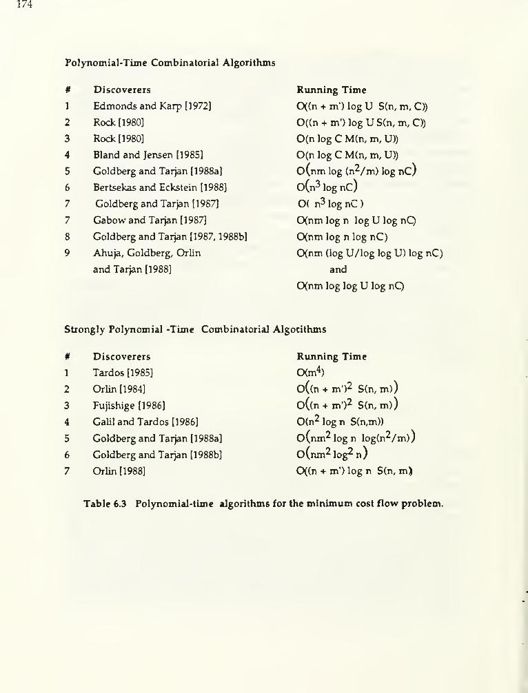
174

Polynomial-Time Combinatorial Algorithms

# Discoverers

1 Edmonds and Karp [1972]

2 Rock [1980]

3 Rock [1980]

4 Bland and Jensen [1985]

5 Goldberg and Tarjan [1988a]

6 Bertsekas and Eckstein [1988]

7 Goldberg and Tarjan [1987]

7 Gabow and Tarjan [1987]

8 Goldberg and Tarjan [1987, 1988b]

9 Ahuja, Goldberg, Orlin

and Tarjan [1988]

Running Time

0((n + m") log U S(n, m, C))

0((n + m') log U S(n, m, O)

0(n log C M(n, m, U))

0(n log C M(n, m, U))

0(nm log irr/nx) log nC)

o(n3 log nC)

0( n^ log nC )

0(nm log n log U log nQ0(nm log n log nC)

0(nm (log U/log log U) log nC)

and

0(nm log log U log nQ

Strongly Polynomial -Time Combinatorial Algorithms

#

175

For the sake of comparing the polynomial and strongly polynomial-time

algorithms, we invoke the similarity assumption. For problems that satisfy the

similarity assumption, the best bounds for the shortest path and maximum flow

problems are:

Polynomial-Time Bounds Discoverers

S(n,m, C) = min (m log log C, m + rh/logC ) Johnson [1982], and

Ahuja, Mehlhom, Orlin and Tarjan

[1988]

^%rT^gTJM(n, m, C) = nm log

[ ^— + 2J

Ahuja, Orlin and Tarjan [1987]

Strongly Polynomial -Time Bounds Discoverers

S(n, m) = m + n log n Fredman and Tarjan [1984]

M(n, m) = nm log (n^/m) Goldberg and Tarjan [1986]

Using capacity and right-hand-side scaling, Edmonds and Karp [1972]

developed the first (weakly) polynomial-time eilgorithm for the minimum cost flow

problem. The RHS-scaling algorithm presented in Section 5.7, which L> a Vciriant of

the Edmonds-Karp algorithm, was suggested by Orlin [1988]. The scaling technique

did not initially capture the interest of many researchers, since they regarded it as

having little practical utility. However, researchers gradually recognized that the

scaling technique has great theoretical value as well as potential practical significance.

Rock [1980] developed two different bit-scaling algorithms for the minimum cost

flow problem, one using capacity scaling and the other using cost scaling. This cost

scaling algorithm reduces the minimum cost flow problem to a sequence of

0(n log C) maximum flow problems. Bland and Jensen [1985] independently

discovered a similar cost scaling algorithm.

The pseudoflow push algorithms for the minimum cost flow problem

discussed in Section 5.8 use the concept of approximate optimality, introduced

independently by Bertsekas [1979] and Tardos [1985]. Bertsekas [1986] developed the

first pseudoflow push algorithm. This algorithm was pseudopolynomial-time.

Goldberg and Tarjan [1987] used a scaling technique on a variant of this algorithm to

obtain the generic pseudoflow push algorithm described in Section 5.8. Tarjan [1984]

proposed a wave algorithm for the maximum flow problem. The wave algorithm

176

for the minimum cost flow problem described in Section 5.8 , which was developed

independently by Goldberg and Tarjan [1987] and Bertsekas and Eckstein [1988], relies

upon similar ideas. Using a dynamic tree data structure in the generic pseudoflow

push algorithm, Goldberg and Tarjan [1987] obtained a computational time bound of

0(nm log n log nC). They also showed that the minimum cost flow problem cam be

solved using 0(n log nC) blocking flow computations. (The description of Dinic's

algorithm in Section 6.3 contains the definition of a blocking flow.) Using both

finger tree (see Mehlhom [1984]) and dynamic tree data structures, Goldberg and

Tarjan [1988a] obtained an 0(nm log (n^/m) log nC) bound for ^he wave algorithm.

These algorithms, except the wave algorithm, required sophisticated data

structures that impose a very high computational overhead. Although the wave

algorithm is very practical, its worst-case running time is not very attractive. This

situation has prompted researchers to investigate the possibility of improving the

computational complexity of minimum cost flow algorithms without using any

complex data structures. The first success in this direction was due to Gabow and

Tarjan [1987], who developed a triple scaling algorithm running in time 0(nm log n

log U log nC). The second success was due to Ahuja, Goldberg, Orlin and Tarjan

[1988], who developed the double scaling algorithm. The double scaling algorithm,

as described in Section 5.9, runs in 0(nm log U log nC) time. Scaling costs by an

appropriately larger factor improves the algorithm to 0(nm(log U/log log U) log nC)

,

and a dynamic tree implementation improves the bound further to 0(nm log log U

log nC). For problems satisfying the similarity assumption, the double scaling

algorithm is faster than all other algorithms for all network topologies except for

very dense networks; in these instances, algorithms by Goldberg and Tarjan appear

more attractive.

Goldberg and Tarjan [1988b] and Barahona and Tardos [1987] have developed

other polynomial-time algorithms. Both the algorithms are based on the negative

cycle algorithm due to Klein [1967]. Goldberg and Tarjan [1988b] showed that if the

negative cycle algorithm always augments along flow a minimum mean cycle (a

cycle W for which V Cj; / |W | is minimum), then it is strongly polynomial-time.

(i,j) 6 WGoldberg and Tarjan described an implementation of this approach running in time

0(nm(log n) minflog nC, m log n)). Barahona and Tardos [1987], analyzing an

algorithm suggested by Weintraub [1974], showed that if the negative cycle algorithm

177

augments flow along a cycle with maximum improvement in the objective function,

then it performs 0(m log mCU) iterations. Since identifying a cycle with maximum

improvement is difficult (i.e., NP-hard), they describe a method (based upon solving

an auxiliary assignment problem) to determine a disjoint set of augmenting cycles

with the property that augmenting flows along these cycles improves the flow cost

by at least as much as augmenting flow along any single cycle. Their algorithm runs

in 0(.Tr\^ log (mCU) S(n, m, O) time.

Edmonds and Karp [1972] proposed the first polynomial-time algorithm for

the minimum cost flow problem, and also highlighted the desire to develop a

strongly polynomial-time algorithm. This desire was motivated primarily by

theoretical considerations. (Indeed, in practice, the terms log C and log U typically

range from 1 to 20, and are sublinear in n.) Strongly polynomial-time algorithms are

theoretically attractive for at least two reasons: (i) they might provide, in principle,

network flow algorithms that can run on real valued data as well as integer valued

data, and (ii) they might, at a more fundamental level, identify the source of the

underlying complexity in solving a problem; i.e., are problems more difficult or

equally difficult to solve as the values of the tmderlying data becomes increasingly

larger?

The first strongly polynomial-time minimum cost flow algorithm is due to

Tardos [1985]. Several researchers including Orlin [1984], Fujishige [1986], Galil and

Tardos [1986], and Orlin [1988] provided subsequent improvements in the running

time. Goldberg and Tarjan [1988a] obtained another strongly polynomial time

algorithm by slightly modifying their pseudoflow push algorithm. Goldberg and

Tarjan [1988b] also show that their algorithm that proceeds by cancelling minimvun

mean cycles is also strongly polynomial time. Currently, the fastest strongly

polynomial-time algorithm is due to Orlin [1988]. This algorithm solves the

minimum cost flow problem as a sequence of 0(min(m log U, m log n)) shortest path

problems. For very sparse networks, the worst-case running time of this algorithm is

nearly as low cis the best weakly polynomieil-time algorithm, even for problems that

satisfy the similarity assumption.

Interior point linear programming algorithms are another source of

polynomial-time algorithms for the minimum cost flow problem. Kapoor and

Vaidya [1986] have shown that Karmarkar's [1984] algorithm, when applied to the

minimum cost flow problem performs 0(n^-^ mK) operations, where

178

K = log n + log C + log U. Vaidya [1986] suggested another algorithm for linear

programming that solves the minimum cost flow problem in 0(n^-^ y[m K) time.

Asymptotically, these time bounds are worse than that of the double scaling

algorithm.

At this time, the research community has yet to develop sufficient evidence to

fully assess the computational worth of scaling and interior point linear

programming algorithms for the minimum cost flow problem. According to the

folklore, even though they might provide the best-worst case bounds on running

times, the scaling algorithms eu-e not as efficient as the non-scaling algorithms. Boyd

and Orlin [1986] have obtained contradictory results. Testing the right-hand-side

scaling algorithm for the minimum cost flow problem, they found the scaling

algorithm to be competitive with the relaxation algorithm for some classes of

problems. Bland and Jensen [1985] also reported encouraging results with their cost

scaling algorithm. We believe that when implemented with appropriate speed-up

techniques, scaling algorithms have the potential to be competitive with the best

other algorithms.

6.5 Assignment Problem

The assignment problem has been a popular research topic. The primary

emphasis in the literature has been on the development of empirically efficient

algorithms rather than the development of algorithms with improved worst-case

complexity. Although the research community has developed several different

algorithms for the assignment problem, many of these algorithms share common

features. The successive shortest path algorithm, described in Section 5.4 for the

minimum cost flow problem, appears to lie at the heart of many assignment

algorithms. This algorithm is implicit in the first assignment algorithm due to Kuhn

[1955], known as the Hungarian method, and is explicit in the papers by Tomizava

[1971] and Edmonds and Karp [1972].

When applied to an assignment problem on the network G = (N^ u N2 , A)

,

the successive shortest path algorithm operates as follows. To use this solution

approach, we first transform the assignment problem into a minimum cost flow

problem by adding a source node s and a sink node t, and introducing arcs (s,i) for all

i€N|, and (j,t) for all J€N2 ; these arcs have zero cost and unit capacity. The

algorithm successively obtains a shortest path from s to t with respect to the lir«;ar

179

programming reduced costs, updates the node potentials, and augments one unit of

flow along the shortest path. The algorithm solves the assignment problem by n

applications of the shortest path algorithm for nonnegative arc lengths and runs in

0(nS(n,m,C)) time, where S(n,m,C) is the time needed to solve a shortest path

problem. For a naive implementation of Dijkstra's algorithm, S(n,m,C) is O(n^) and

for a Fibonacci heap implementation it is 0(m+nlogn). For problems satisfying the

similarity assumption, S(n,m,C) is min(m log log C, m+nVlogC}.

The fact that the assignment problem can be solved as a sequence of n shortest

path problems with arbitrary arc lengths follows from the works of Jewell [1958], Iri

[1960] and Busaker and Gowen [1961] on the minimum cost flow problem. However,

Tomizava [1971] and Edmonds and Karp [1972] independently pointed out that

working with reduced costs leads to shortest path problems with nonnegative arc

lengths. Weintraub and Barahona [1979] worked out the details of Edmonds-Karp

algorithm for the assignment problem. The more recent threshold assignment

algorithm by Glover, Glover and Klingman [1986] is also a successive shortest path

algorithm which integrates their threshold shortest path algorithm (see Glover,

Glover and Klingman [1984]) with the flow augmentation process. Carraresi and

Sodini [1986] also suggested a similar threshold assignment algorithm.

Hoffman and Markowitz [1963] pointed out the transformation of a shortest

path problem to an assignment problem.

Kuhn's [1955] Hungarian method is the primal-dual version of the successive

shortest path algorithm. After solving a shortest path problem and updating the

node potentials, the Hungarian method solves a (particularly simple) maximum

flow problem to send the maximum possible flow from the source node s to the sink

node t using arcs vdth zero reduced cost. Whereas the successive shortest path

problem augments flow along one path in an iteration, the Hungarian method

augments flow along all the shortest paths from the source node to the sink node. If

we use the labeling algorithm to solve the resulting maximum flow problems, then

these applications take a total of 0(nm) time overall, since there are n augmentatior\s

and each augmentation takes 0(m) time. Consequently, the Hungarian method, too,

runs in 0(nm + nS(n,mC)) = 0(nS(n,m,C)) time. (For some time after the

development of the Hungarian method as described by Kuhn, the research

community considered it to be O(n^) method. Lawler [1976] described an Oiri^)

180

implementation of the method. Subsequently, many researchers realized that the

Hungarian method in fact runs in 0(nS(n,m,C)) time.) Jonker and Volgenant [1986]

suggested some practical improvements of the Hungarian method.

The relaxation approach for the minimum cost flow problem is due to E>inic

and Kronrod (1969], Hung eind Rom [1980] and Engquist [1982]. This approach is

closely related to the successive shortest path algorithm. Both approaches start writh

an infeasible assignment and gradually make it feasible. The major difference is in

the nature of the infeasibility. The successive shortest path algorithm maintains a

solution w^ith unassigned persons and objects, and with no person or object

overassigned. Throughout the relaxation algorithm, every person is assigned, but

objects may be overassigned or unassigned. Both the algorithms maintain optimality

of the intermediate solution and work toward feasibility by solving at most n shortest

path problems with nonnegative arc lengths. The algorithms of Dinic and Kronrod

[1969] and Engquist [1982] are essentially the same as the one we just described, but

the shortest path computations are somewhat disguised in the paper of Dinic and

Kronrod [1969]. The algorithm of Hung and Rom [1980] maintains a strongly feaisible

basis rooted at an overassigned node and, after each augmentation, reoptimizes over

the previous basis to obtain another strongly feaisible basis. All of these algorithms

run in 0(nS(n,m,C)) time.

Another algorithm worth mentioning is due to Balinski and Gomory [1964].

This algorithm is a primal algorithm that maintains a feasible assignment and

gradually converts it into an optimum assignment by augmenting flows along

negative cycles or by modifying node potentials. Derigs [1985] notes that the shortest

path computations vmderlie this method, and that it rurrs in 0(nS(n,m,C)) time.

Researchers have also studied primal simplex algorithms for the assignment

problem. The basis of the assignment problem is highly degenerate; of its 2n-l

variables, only n are nonzero. Probably because of this excessive degeneracy, the

mathematical programming community did not conduct much research on the

network simplex method for the assignment problem until Barr, Glover and

Klingman [1977a] devised the strongly feasible basis technique. These authors

developed the details of the network simplex algorithm when implemented to

maintain a strongly feasible basis for the assignment problem; they also reported

encouraging computational results. Subsequent research focused on developing

ISl

polynomial-time simplex algorithms. Roohy-Laleh [1980] developed a simplex pivot

rule requiring O(n^) pivots. Hung [1983] describes a pivot rule that performs at most

O(n^) consecutive degenerate pivots and at most 0(n log nC) nondegenerate pivots.

Hence, his algorithm performs 0(n^log nC) pivots. Akgul [1985b] suggested another

primal simplex algorithm performing O(n^) pivots. This algorithm essentially

amounts to solving n shortest path problems and runs in 0(nS(n,m,C)) time.

Orlin [1985] studied the theoretical properties of Dantzig's pivot rule for the

netvk'ork simplex algorithm and showed that for the eissignment problem this rule

requires O(n^lognC) pivots. A naive implementation of the algorithm runs in

0(n^m log nC). Ahuja and Orlin [1988] described a scaling version of Dantzig's pivot

rule that performs 0(n^log C) pivots and can be implemented to run in 0(nm log C)

time using simple data structures. The algorithm essentially consists of pivoting in

any arc with sufficiently large reduced cost. The algorithm defines the term

"sufficiently large" iteratively; initially, this threshold value equals C and within

O(n^) pivots its value is halved.

Balinski [1985] developed the signature method, which is a dual simplex

algorithm for the eissignment problem. (Although his basic algorithm maintains a

dual feasible basis, it is not a dual simplex algorithm in the traditional sense because

it does not necessarily increase the dual objective at every iteration; some variants of

this algorithm do have this property.) Balinski's algorithm performs O(n^) pivots

and runs in O(n^) time. Goldfarb [1985] described some implementations of

Balinski's algorithm that run in O(n^) time using simple data structures and in

0(nm + n^log n) time using Fibonacci heaps.

The auction algorithm is due to Bertsekas and uses basic ideas originally

suggested in Bertsekas [1979]. Bertsekas and Eckstein [1988] described a more recent

version of the auction algorithm. Out presentation of the auction algorithm tmd its

analysis is somewhat different that the one given by Bertsekas and Eckstein [1988].

For example, the algorithm we have presented increases the prices of the objects by

one unit at a time, whereas the algorithm by Bertsekas and Eckstein increases prices

by the maximum amount that preserves e-optimality of the solution. Bertsekas

[1981] has presented another algorithm for the assignment problem which is in fact a

specialization of his relaxation algorithm for the minimum cost flow problem (see

Bertsekas [1985]).

Currently, the best strongly polynomial-time bound to solve the assignment

problem is 0(nm + n^ log n) which is achieved by many assignment algorithms.

Scaling algorithms can do better for problems that satisfy the similarity assumption.

Gabow [1985] , using bit-scaling of costs, developed the first scciling algorithm for the

assignment problem. His algorithm performs O(log C) scaling phases and solves

each phase in OCn'^'^m) time, thereby achieving jm OCn'^' ^m log C) time bound.

Using the concept of e-optimality, Gabow and Tarjan [1987] developed another scaling

algorithm running in time 0(n^' ^m log nC). Observe that the generic pseudoflow

push algorithm for the minimum cost flow problem described in Section 5.8 solves

the assignment problem in 0(nm log nC) since every push is a saturating push.

Bertsekas and Eckstein [1988] showed that the scaling version of the auction

algorithm runs in 0(nm log nC). Section 5.11 has presented a modified version of

this algorithm in Orlin and Ahuja [1988]. They also improved the time bound of the

auction algorithm to 0(n^'^m lognC). This time bound is comparable to that of

Gabow and Tarjan 's algorithm, but the two algorithms would probably have different

computational attributes. For problems satisfying the similarity assumption, these

two algorithms achieve the best time boimd to solve the assignment problem

without using any sophisticated data structure.

As mentioned previously, most of the research effort devoted to assignment

algorithms has stressed the development of empirically faster algorithms. Over the

years, many computational studies have compared one algorithm with a few other

algorithms. Some representative computational studies are those conducted by Barr,

Glover and Klingman [1977a] on the network simplex method, by McGinnis [1983]

and Carpento, Martello and Toth [1988] on the primal-dual method, by Engquist

[1982] on the relaxation methods, and by Glover et al. [1986] and Jonker and

Volgenant [1987] on the successive shortest path methods. Since no paper has

compared all of these zilgorithms, it is difficult to assess their computational merits.

Nevertheless, results to date seem to justify the following observations about the

algorithms' relative performance. The primal simplex algorithm is slower than the

primal-dual, relaxation and successive shortest path algorithms. Among the latter

three approaches, the successive shortest path algorithms due to Glover et al. [1986]

and Jonker and Volgenant [1987] appear to be the fastest. Bertsekas and Eckstein

[1988] found that the scaling version of the auction algorithm is competitive with

Jonker and Volgenant's algorithm. Carpento, Martello and Trlh [1988] present

183

several FORTRAN implementations of assignment algorithms for dense and sparse

cases.

6.6 Other Topics

Our discussion in this paper has featured single commodity network flow

problems with linear costs. Several other generic topics in the broader problem

domain of network optimization are of considerable theoretical and practical interest.

In particular, four other topics deserve mention: (i) generalized network flows;

(ii) convex cost flows; (iii) multicommodity flows; and (iv) network design. We

shall now discuss these topics briefly.

Generalized Network Flows

The flow problems we have considered in this chapter assume that arcs

conserve flows, i.e., the flow entering an arc equals the flow leaving the arc. In

models of generalized network flows, arcs do not necessarily conserve flow. If xj:

units of flow enter an arc (i, j), then Tj: Xj: units "arrive" at node j; Tj; is a

nonnegative flow multiplier dissociated with the arc. If < rj: < 1, then the arc is

lossy and, if 1 < Tj; < «>, then the arc is gainy. In the conventional flow networks, Tjj =

1 for all arcs. Generalized network flows arise in may application contexts. For

example, the multiplier might model pressure losses in a water resource network or

losses incurred in the transportation of perishable goods.

Researchers have studied several generalized network flow problems. An

extension of the conventional maximum flow problem is the generalized maximum

flow problem which either maximizes the flow out of a source node or maximizes

the flow into a sink node (these two objectives are different!) The source version of

the problem can be states as the following linear program.

Maximize v^ (6ia)

subject to

X "ij - S "'ji'^ji = K'if» = s

{j: (i,j) € A) {j: (j,i) € A) S 0, if i ?t s,t, for aU i E N (6.1b)

[vj, if i = t

184

< x^j < uj: , for all (i, j) e A.

Note that the capacity restrictions apply to the flows entering the arcs.

Further, note that Vg is not necessarily equal to v^, because of flow losses and gains

within arcs.

The generalized maximum flow problem has many similarities with the

minimum cost flow problem. Extended versions of the successive shortest path

algorithm, the negative cycle algorithm, and the primal-dual algorithm for the

minimum cost flow problem apply to the generalized maximum flow problem. The

paper by Truemper [1977] surveys these approaches. These algorithms, however, are

not pseudopolynomial-time, mainly because the optimal arc flows and node

potentials might be fractional. The recent paper by Goldberg, Plotkin and Tardos

[1986] describes the first polynomial-time combinatorial algorithms for the

generalized maximum flow problem.

In the generalized minimum cost flow problem, which is an extension of the

ordinary minimum cost flow problem, we wish to determine the minimum cost

flow in a generalized network satisfying the specified supply/demand requirements

of nodes. These are three main approaches to solve this problem. The first approach,

due to Jewell [1982], is essentially a primal-dual algorithm. The second approach is

the primal simplex algorithm studied by Elam, Glover and Klingman [1979] among

others. Elam et al. find their implementation to be very efficient in practice; they

find that it is about 2 to 3 times slower than their implementations for the ordinary

minimum cost flow algorithm. The third approach, due to Bertsekeis and Tseng

[1988b], generalizes their minimum cost flow relaxation algorithm for the

generalized minimum cost flow problem.

Convex Cost Flows

We shall restrict this brief discussion to convex cost flow problems with

separable cost functions, i.e., the objective function can be written in the form

V Cjj (x^j). Problems containing nonconvex nonseparable cost terms such as xj2

(i,j) e A

X-J3 are substantially more difficult to solve and continue to pose a significant

challenge for the mathematical programming community. Even problems with

nonseparable, but convex objective functions are more difficult to solve; typically.

185

analysts rely on the general nonlinear programming techniques to solve these

problems. The separable convex cost flow problem has the follow^ing formulation:

Minimize V Cj; (xj;) (6.2a)

(i,j) e A

subject to

Y ^i]- S ''ji

= ^^'^' ^°^ all i € N, (6.2b)

{j: (i,j) € A {j: (j,i) e A

< x^j < Ujj , for all (i, j) e A. (62c)

In this formulation, Cj; (xjj) for each (i,j) e A, is a convex function. The

research community has focused on two classes of separable convex costs flow

problems: (i) each Cj; (xjj) is a piecewise linear function; of (ii) each Cj; (xj;) is a

continuously differentiate function. Solution techniques used to solve the two

classes of problems are quite different.

There is a well-known technique for transforming a separable convex

program with piecewise linear functions to a linear program (see, e.g., Bradley, Hax

and Magnanti [1972]). This transformation reduces the convex cost flow problem to a

standard minimum cost flow problem: it introduces one arc for each linear segment

in the cost functions, thus increasing the problem size. However, it is possible to

carry out this transformation implicitly and therefore modify many minimum cost

flow algorithms such as the successive shortest path algorithm, negative cycle

algorithm, primal-dual and out-of-kilter algorithms, to solve convex cost flow

problems without increasing the problem size. The paper by Ahuja, Batra, and Gupta

[1984] illustrates this technique and suggests a pseudopolynomial time algorithm.

Observe that it is possible to use a piecewise linear function, with linear

segments chosen (if necessary) with sufficiently small size, to approximate a convex

function of one variable to any desired degree of accuracy. More elaborate

alternatives are possible. For example, if we knew the optimal solution to a separable

convex problem a priori (which of course, we don't), then we could solve the

problem exactly using a linear approximation for any arc (i, j) with only three

186

breakpoints: at 0, Uj; and the optimal flow on the arc. Any other breakpoint in the

linear approximation would be irrelevant and adding other points would be

computationally wasteful. This observation has prompted researchers to devise

adaptive approximations that iteratively revise the linear approximation beised upon

the solution to a previous, coarser, approximation. (See Meyer [1979] for an example

of this approach). If we were interested in only integer solutions, then we could

choose the breakpoints of the linear approximation at the set of integer values, and

therefore solve the problem in pseudopolynomial time.

Researchers have suggested other solution strategies, using ideas from

nonlinear progamming for solving this general separable convex cost flow problems.

Some important references on this topic are Ali, Helgason and Kennington [1978],

Kennington and Helgason [1980], Meyer and Kao [1981], Dembo and Klincewicz

[1981], Klincewicz [1983], Rockafellar [1984], Florian [1986], and Bertsekas, Hosein and

Tseng [1987].

Some versions of the convex cost flow problems can be solved in polynomial

time. Minoux [1984] has devised a polynomial-time algorithm for one of its special

cases, the mininimum quadratic cost flow problem. Minoux [1986] has also

developed a polynomial-time algorithm to obtain an integer optimum solution of

the convex const flow problem.

Muticommodity Flows

Multicommodity flow problems arise when several commodities use the

same underlying network, but share common arc capacities. In this section, we state

a linear programming formulation of the multicommodity minimum cost flow

problem and point the reader to contributions to this problem and its specializations.

Suppose that the problem contains r distinct commodities numbered 1

through r. Let b*^ denote the supply/demand vector of commodity k. Then the

multicommodity minimum cost flow problem can be formulated as follows:

^k k

Minimize V V c^: x^- (6.3a)

1^=1 (i,j)e A

subject to

187

k k kX;; - V

''ii~

^i ' ^OT a\] i and k, (6.3b)1]

{j: (i,j) e A) {j: (i,j) e A

' ky X.. < u:j, for all (i,j),,

(63c)

ktl'^ ^

k k< Xj. < u- , for all (i,j) and all k . (6.3d)

k kIn this formulation, x-- and c-- represent the amont of flow and the unit cost

of flow for commodity k on arc (i,j). As indicated by the "bundle constraints" (6.3c),

the total flow on any arc cannot exceed its capacity. Further, as captured by (6.3d), the

model contains additional capacity restrictions on the flow of each commodity on

each arc.

Observe that if the multicommodity flow problem does not contain bundle

constraints, then it decomposes into r single commodity minimum cost flow

problems, one for each commodity. With the presence of the bundle corxstraints

(6.3c), the essential problem is to distribute the capacity of each arc to individual

commodities in a way that minimizes overall flow costs.

We first consider some special cases. The multicommodity maximum flow

problem is a special instance of (6.3). In this problem, every commodity k has a

source node and a sink node, represented respectively by s*^ and tK The objective is

to maximize the sum of flows that can be sent from s*^ to t*^ for all k. Hu [1963]

showed how to solve the two-commodity maximum flow problem on an undirected

network in pseudopolynomial time by a labeling algorithm. Rothfarb, Shein and

Frisch [1968] showed how to solve the multicommodity maximum flow problem

with a common source or a common sink by a single application of any maximum

flow algorithm. Ford and Fulkerson [1958] solved the general multicommodity

maximum flow problem using a column generation algorithm. Dantzig and Wolfe

[1960] subsequently generalized this decomposition approach to linear programming.

Researchers have proposed three basic approaches for solving the general

multicommodity minimum cost flow problems: price-directive decomposition,

resource-directive decomposition and partitioning methods. We refer the reader to

188

the excellent surveys by Assad [1978] and Kennington [1978] for descriptions of these

methods. The book by Kennington and Helgason [1980] describes the details of a

primal simplex decomposition algorithm for the multicommodity minimum cost

flow problem. Unfortunately, algorithmic developments on the multicommodity

minimum cost flow problem have not progressed at nearly the pace as the progress

made on the single commodity minimum cost flow problem. Although specialized

primal simplex software can solve the single commodity problem 10 to 100 times

faster than the general purpose linear programming systems, the algorithms

developed for the multicommodity minimum cost flow problems generally solve

thse problems about 3 times faster than the general purpose software (see Ali et al.

[1984]).

Network Design

We have focused on solution methods for finding optimal routings in a

network; that is, on analysis rather than synthesis. The design problem is of

considerable importance in practice and has generated an extensive literature of its

own. Many design problems can be stated as fixed cost network flow problems:

(some) arcs have an associated fixed cost which is incurred whenever the arc carries

any flow. These network design models contain 0-1 variables yjj that indicate

whether or not an arc is included in the network. Typically, these models involve

kmulticommodity flows. The design decisions yjj and routing decisions x^- are

related by "forcing" constraints of the form

2 ''ii- "ij yij

'^^^ ^" ^^'^^

k=l

which replace the bundle constraints of the form (6.3c) in the convex cost

kmulticommodity flow problem (6.3). These constraints force the flow x^- of each

commodity k on arc (i,j) to be zero if the arc is not included in the network design; if

the arc is included, the constraint on arc (i,j) restricts the total flow to be the arc's

design capacity Ujj Many modelling enhancements are possible; for example, some

constraints may restrict the underlying network topology (for instance, in some

applications, the network must be a tree; in other applications, the network might

189

need alternate paths to ensure reliable operations). Also, many different objective

functions arise in practise. One of the most popular is

""

k kMinimize £ ^ c-

•x^^ + Y. ^V ij

k=l (i^j)e A (i,j) € A

kwhich models commodity dependent per unit routing costs c • (as well zs fixed costs

Fjj for the design arcs).

Usually, network design problems require solution techniques from any

integer programming and other type of solution methods from combinatorial

optimization. These solution methods include dynamic programming, dual ascent

procedures, optimization-based heuristics, and integer programming decomposition

(Lagrangian relaxation. Benders decomposition) as well as emerging ideas from the

field of polyhedral combinatorics. Magnanti and Wong [1984] and Minoux [1985,

1987] have described the broad range of applicability of network design models and

summarize solution methods for these problems as well as many references from the

network design literature. Nemhauser and Wolsey [1988] discuss many underlying

methods from integer programming and combinatorial optimization.

Acknowledgments

We are grateful to Michel Goemans, Hershel Safer, Lav^ence Wolsey ,Richard

Wong and Robert Tarjan for a careful reading of the manuscript and many useful

suggestions. We are particularly grateful to William Cunningham for many

valuable and detailed comments.

The research of the first and third authors was supported in part by the

Presidential Young Investigator Grant 8451517-ECS of the National Science

Foundation, by Grant AFOSR-88-0088 from the Air Force Office of Scientific

Research, and by Grants from Analog Devices, Apple Computer, Inc., and Prime

Computer.

190

References

Aashtiani, H.A., and T. L. Magnanti. 1976. Implementing Prin\al-E>ual Network

Flow Algorithms. Technical Report OR 055-76, Operations Research Center, M.I.T.,

Cambridge, MA.

Aho, A.V. , J.E. Hop>croft, and J.D. Ullman. 1974. The Design and Analysis of Computer

Algorithms. Addison-Wesley, Reading, MA.

Ahuja, R. K., J. L. Batra, and S. K. Gupta. 1984. A Parametric Algorithm for the

Convex Cost Network Flow and Related Problems. Euro. ].of Oper. Res. 16, 222-25

Ahuja, R.K., A.V. Goldberg, J.B. Orlin, and R.E. Tarjan. 1988. Finding

Minimum-Cost Rows by Double Scaling. Working Paper No. 2047-88, Sloan School

of Management, M.I.T., Cambridge, MA.

Ahuja, R.K., M. Kodialam, and J.B. Orlin. 1988. Personal Communication.

Ahuja, R.K., K. Mehlhom, J.B. Orlin, and R.E. Tarjan. 1988. Faster Algorithms for

the Shortest Path Problem. Technical Report No. 193, Operations Research Center,

M.I.T., Cambridge, MA.

Ahuja, R.K., and J.B. Orlin. 1987. A Fast and Simple Algorithm for the Maximum

Flow Problem. Working Paper 1905-87, Sloan School of Management, M.I.T.,

Cambridge, MA. 1987. To appear in Oper. Res.

Ahuja, R.K., and J.B. Orlin. 1988. Improved Primal Simplex Algorithms for the

Shortest Path, Assignment and Minimum Cost Flow Problems. To appear.

Ahuja, R.K., J.B. Orlin, C. Stein, and R.E. Tarjan. 1988. Improved Algorithms for

Bipartite Network Flow Problen«. To appear.

Ahuja, R.K., J.B. Orlin, and R.E. Tarjan. 1988. Improved Time Bounds for the

Maximum Flow Problem. Working Paper 1966-87, Sloan School of Management,

M.I.T., Cambridge, MA.

Akgul, M. 1985a. Shortest Path and Simplex Method. Research Report, Department

of Computer Science and Operations Research, North Carolina State University,

Raleigh, N.C.

191

Akgul, M. 1985b. A Genuinely Polynomial Primal Simplex Algorithm for the

Assignment Problem. Research Report, Department of Computer Science and

Operations Research, North Carolina State University, Raleigh, N.C.

Ali,I., D. Bamett, K. Farhangian, J. Kennington, B. Patty, B. Shetty, B. McCarl and P.

Wong. 1984. Multicommodity Network Problems: Applications and Computations.

LIE. Trans. 16,127-134.

Ali, A. I., R. V. Helgason, and J. L. Kennington. 1978. The Convex Cost Netwrork

Flow Problem: A State-of-the-Art Survey. Technical Report OREM 78001, Southern

Methodist University, Texeis.

Armstrong, R.D., D. Klingman, and D. Whitman. 1980. Implementation and

Analysis of a Variant of the Dual Method for the Capacitated Transshipment

Problem. Euro. J. Oper. Res. 4, 403-420.

Assad, A. 1978. Multicommodity Network Flows - A Survey. Networks 8,37-91.

Balinski, M.L. 1985. Signature Methods for the Assignment Problem. Oper. Res. 33,

527-536.

Balinski, M.L., and R.E. Comory. 1964. A Primal Method for the Assignment and

Transportation Problems. Man. Sci. 10, 578-593.

Barahona, F., and E. Tardos. 1987. Note on Weintraub's Minimum Cost Flow

Algorithm. Research Report, Dept. of Mathematics, M.I.T., Cambridge, MA.

Baratz, A.E. 1977. Construction and Analysis of a Network Flow Problem Which

Forces Karzanov Algorithm to O(n^) Running Time. Technical Report TM-83,

Laboratory for Computer Science, MIT, Cambridge, MA.

Ban, R., F. Glover, and D. Klingman. 1977a.. The Alternating Path Basis Algorithm

for the Assignment Problem. Math. Prog. 12, 1-13.

Barr, R., F. Glover, and D. Klingman. 1977b. A Network Augmenting Path Basis

Algorithm for Transshipment Problems. Proceedings of the International Symposium on

External Methods and System Analysis.

192

Barr, R., F. Glover, and D. Klingman. 1978. Generalized Alternating Path Algorithm

for Transportation Problems. Euro. ]. Oper. Res. 2, 137-144.

Barr, R., P. Glover, and D. Klingman. 1979. Enhancement of Spanning Tree Labeling

Procedures for Network Optimization. INFOR 17, 16-34.

Bazaraa, M., and J.J. Jarvis. 1978. Linear Programming and Network Flows. John

Wiley & Sons.

Bellman, R. 1958. On a Routing Problem. QuaH. Appl. Math. 16, 87-90.

Berge, C., and A. Ghouila-Houri. 1962. Programming, Games and Transportation

Networks. John Wiley & Sons.

Bertsekas, D.P. 1979. A Distributed Algorithm for the Assignment Problem.

Working Paper, Laboratory for Information Decision Systems, M.I.T., Cambridge,

MA.

Bertsekas, D.P. 1981. A Nev^ Algorithm for the Assignment Problem. Math. Prog. 21,

152-171.

Bertsekas, D. P. 1985. A Unified Framev^ork for Primal-Dual Methods in Minimum

Cost Network Flow Problems. Math. Prog. 32, 125-145.

Bertsekas, D.P. 1986. Distributed Relaxation Methods for Linear Network Flow

Problems. Proc. of 25th IEEE Conference on Decision and Control, Athens, Greece.

Bertsekas, D. P. 1987. The Auction Algorithm: A Distributed Relaxation Method for

the Assignment Problem. Report LIDS-P-1653, Laboratory for Information Decision

systems, M.I.T., Cambridge, MA. Also in Annals of Operations Research 14, 105-123.

Bertsekas, D.P., and J. Eckstein. 1988. IXial Coordinate Step Methods for Linear

Network Flow Problems. To appear in Math. Prog., Series B.

Bertsekas, D., and R. Gallager. 1987. Data Networks. Prentice-Hall.

Bertsekas, D. P., P. A. Hosein, and P. Tseng. 1987. Relaxation Methods for Network

Flow Problems with Convex Arc Costs. . SIAM J. of Control and Optimization

25,1219-1243.

193

Bertsekas, D.P., and P. Tseng. 1988a. The Relax Codes for Linear Minimum Cost

Network Flow Problems. In B. Simeone, et al. (ed.), FORTRAN Codes for Network

Optimization. As Annals of Operations Research 13, 125-190.

Bertsekas, D.P., and P. Tseng. 1988b. Relaxation Methods for Minimum Cost

Ordinary and Generalized Network Flow Problems. Oper. Res. 36, 93-114.

Bland, R.G., and D.L. Jensen. 1985. On the Computational Behavior of a

Polynomial-Time Network Flow Algorithm. Technical Report 661, School of

Operations Research and Industrial Engineering, Cornell University, Ithaca, N.Y.

Boas, P. Van Emde, R. Kaas, and E. Zijlstra. 1977. Design and Implementation of an

Efficient Priority Queue. Math. Sys. Theory 10, 99-127.

Bodin, L. D., B. L. Golden, A. A. Assad, and M. O. Ball. 1983. Routing and Scheduling

of Vehicles and Crews. Comp. and Oper. Res. 10, 65-211.

Boyd, A., and J.B. Orlin. 1986. Personal Communication.

Bradley, G., G. Brown, and G. Graves. 1977. Design and Implementation of Large

Scale Primal Transshipment Algorithms. Man. Sri. 21, 1-38.

Bradley, S. P., A. C. Hax, and T. L. Magnanti. 1977. Applied Mathematical

Programming. Addison-Wesley.

Busaker, R.G., and P.J. Gowen. 1961. A Procedure for Determining a Family of

Minimal-Cost Network Flow Patterns. O.R.O. Technical Report No. 15, Operational

Research Office, John Hopkins University, Baltimore, MD.

Carpento, G., S. Martello, and P. Toth. 1988. Algorithms and Codes for the

Assignment Problem. In B. Simeone et al. (eds.), FORTRAN Codes for Network

Optimization. As Annals of Operations Research 33, 193-224.

Carraresi, P., and C. Sodini. 1986. An Efficient Algorithm for the Bipartite Matching

Problem. Eur. J. Oper. Res. 23, 86-93.

Cheriyan, J. 1988. Parametrized Worst Case Networks for Preflow Push Algorithms.

Technical Report, Computer Science Group, Tata Institute of Fundamental Research,

Bombay, India.

194

Cheriyan, J., and S.N. Maheshwari. 1987. Analysis of Preflow Push Algorithms for

Maximum Network Flow. Technical Report, Dept. of Computer Science and

Engineering, Indian Institute of Technology, New Delhi, India.

Cherkasky, R.V. 1977. Algorithm for Cor\struction of Maximum Flow in Networks

with Complexity of OCV^ Vl ) Operation, Mathematical Methods of Solution of

Economical Problems 7, 112-125 (in Russian).

Cheung, T. 1980. Computational Comparison of Eight Methods for the Mzocimum

Network Flow Problem. ACM Trans, on Math. Software 6, 1-16.

Christophides, N. 1975. Graph Theory : An Algorithmic Approach. Academic Press.

Cunningham, W.H. 1976. A Network Simplex Method. Mafft. Pro^. 11, 105-116.

Cunningham, W.H. 1979. Theoretical Properties of the Network Simplex Method.

Math, of Oper. Res. 4, 196-208.

Dantzig, G.B. 1951. Application of the Simplex Method to a Transportation Problem.

In T.C. Koopmans (ed.). Activity Analysis of Production and Allocation, John Wiley &

Sons, Inc., 359-373.

Dantzig, G.B. 1955. Upper Bounds, Secondary Constraints, and Block Triangularity

in Linear Programming. Economeirica 23, 174-183.

Dantzig, G.B. 1960. On the Shortest Route through a Network. Man. Sd. 6, 187-190.

Dantzig, G.B. 1962. Linear Programming and Extensions. Princeton University Press,

Princeton, NJ.

Dantzig, G.B. 1967. All Shortest Routes in a Graph. In P. Rosenthiel (ed.), Theory of

Graphs, Gordon and Breach, NY, 91-92.

Dantzig, G.B., and D.R. Fulkerson. 1956. On the Max-Flow Min-Cut Theorem of

Networks. In H.W. Kuhn and A.W. Tucker (ed.). Linear Inequalities and Related

Systems, Annals of Mathematics Study 38, Princeton University Press, 215-221.

Dantzig, G. B., and P. Wolfe. 1960. Decomposition Principle for Linear Programs.

Oper. Rfs. 8, 101-111.

195

Dembo, R. S., and J. G. Klincewicz. 1981. A Scaled Reduced Gradient Algorithm for

Network Flow Problen\s with Convex Separable Costs. Math. Prog. Study 15, 125-147.

Deo, N., and C Pang. 1984. Shortest Path Algorithms: Taxonomy and Annotation.

Networks 14, 275-323.

Denardo, E.V., and B.L. Fox. 1979. Shortest-Route Methods: 1. Reaching, Pruning

and Buckets. Oper. Res. 27, 161-186.

Derigs, U. 1985. The Shortest Augmenting Path Method for Solving Assignment

Problems: Motivation and Computational Experience. Annals of Operations Research

4,57-102.

Derigs, U. 1988. Programming in Networks and Graphs. Lecture Notes in Economics

and Mathematical Systems, Vol. 300, Springer-Verlag.

Derigs, U., and W. Meier. 1988. Implementing Goldberg's Max-Flow Algorithm: A

Computational Investigation. Technical Report, University of Bayreuth, West

Germany.

Dial, R. 1969. Algorithm 360: Shortest Path Forest with Topological Ordering.

Comm. ACM 12, 632-633.

Dial, R., F. Glover, D. Kamey, and D. Klingman. 1979. A Computational Arvalysis of

Alternative Algorithms and Labeling Techniques for Finding Shortest Path Trees.

Networks 9, 2-[5-248.

Dijkstra, E. 1959. A Note on Two Problems in Connexion with Graphs. Numeriche

Mathematics 1,269-271.

Dinic, E.A. 1970. Algorithm for Solution of a Problem of Maximum Flow in

Networks with Power Estimation, Soviet Math. Dokl. 11, 1277-1280.

Dinic, E.A., and M.A. Kronrod. 1969. An Algorithm for Solution of the Assignment

Problem. Soviet Maths. Doklady 10, 1324-1326.

Edmonds, J. 1970. Exponential Grov^h of the Simplex Method for the Shortest Path

Problem. Unpublished paper. University of Waterloo, Ontario, Canada.

196

Edmonds, J., and R.M. Karp. 1972. Theoretical Improvements in Algorithmic

Efficiency for Network Flow Problems. /. ACM 19, 248-264.

Elam, J., F. Glover, and D. Klingman. 1979. A Strongly Convergent Primal Simplex

Algorithm for Generalized Networks. Math, of Oper. Res. 4, 39-59.

Elias, P., A. Feiitstein, and C.E. Shannon. 1956. Note on Maximum Flow Through a

Network. IRE Trans, on Infor. Theory TT-2, 117-119.

Engquist, M. 1982. A Successive Shortest Path Algorithm for the Assignment

Problem. INFOR 20, 370-384.

Even, S. 1976. The Max-Flow Algorithm of Dinic and Karzanov: An Exposition.

Technical Report TM-80, Laboratory for Computer Science, M.I.T., Cambridge, MA.

Even, S. 1979. Graph Algorithms. Computer Science Press, Maryland.

Even, S., and R.E. Tarjan. 1975. Network Flow and Testing Graph Connectivity.

SIAM }. Comput. 4, 507-518.

Femandez-Baca, D., and C.U. Martel. 1987. On the Efficiency of Maximum Flow

Algorithms on Networks with Small Integer Capacities. Research Report,

Department of Computer Science, Iowa State University, Ames, lA. To appear in

Algorithmica.

Florian, M. 1986. Nonlinear Cost Network Models in Transportation Analysis.

Math. Prog. Study 26, 167-196.

Floyd, R.W. 1962. Algorithm 97: Shortest Path. Comm. >4CM 5, 345.

Ford, L.R., Jr. 1956. Network Flow Theory. Report P-923, Rand Corp., Santa Monica,

CA.

Ford, L.R., Jr., and D.R. Fulkerson. 1956. Maximal Flow through a Network. Canad.

J. Math. 8, 399-404.

Ford, L.R., Jr., and D.R. Fulkerson. 1956. Solving the Trar\sportation Problem. Man.

Sd. 3, 24-32.

197

Ford, L.R., Jr., and D.R. Fulkerson. 1957. A Primal-Dual Algorithm for the

Capacitated Hitchcock Problem. Naval Res. Logist. Quart. 4, 47-54.

Ford, L.R., Jr., and DR. Fulkerson. 1958. Constructing Maximal Dynamic Flows from

Static Flows. Oper. Res. 6, 419-433.

Ford, L., R., and D. R. Fulkerson. 1958. A Suggested Computation for Maximal

Multicommodity Network Flow. Man. Sci. 5, 97-101.

Ford, L.R., Jr., and D.R. Fulkerson. 1962. Flows in Networks.. Princeton University

Press, Princeton, NJ.

Francis, R., and P. Mirchandani (eds.). 1988. Discrete Location Theory. John Wiley &

Sons. To appear.

Frank, H., and I.T. Frisch. 1971. Communication, Transmission, and Transportation

Networks. Addison-Wesley.

Fredman, M. L. 1986. New Bounds on the Complexity of the Shortest Path Problem.

SIAM ]. of Computing 5, 83 - 89.

Fredman, M.L., and R.E. Tarjan. 1984. Fibonacci Heaps and Their Uses in Improved

Network Optimization Algorithms. 25th Annual IEEE Symp. on Found, of Comp. Sci

,

338-346, also in /. ofACM 34(1987), 596-615.

Fujishige, S. 1986. An 0(m^ log n) Capacity-Rounding Algorithm for the Minimum

Cost Circulation Problem: A Dual Framework of Tardos' Algorithm. Math. Prog. 35,

298-309.

Fulkerson, D.R. 1961. An Out-of-Kilter Method for Minimal Cost Flow Problems.

SIAM J. Appl. Math. 9, 18-27.

Fulkerson, D.R., and C.B. Dantzig. 1955. Computation of Maximum Flow in

Networks. Naval Res. Log. Quart. 2, 277-283.

Gabow, H.N. 1985. Scaling Algorithms for Network Problems. J.ofComput.Sys.Sci.

31, 148-168.

Gabow, H.N., and R.E. Tarjan. 1987. Faster Scaling Algorithms for Network

Problems. SIAM ]. Comput. (submitted).

198

GaUl, Z. 1980. OCV^/S E^/^) Algorithm for the Maximum Flow Problem, Acta

Informatica 14, 221-242.

Galil, Z. 1981. On the Theoretical Efficiency of Various Network Flow Algorithms.

Theoretical Comp. Sci. 14, 103-111.

Galil, Z., and A. Naamad. 1980. An 0(VE log^ V) Algorithm for the Maximum

Flow Problem. /. ofComput. Sys. Sci. 21, 203-217.

Galil, Z., and E. Tardos. 1986. An 0(n^(m + n log n) log n) Min-Cost Flow

Algorithm. Proc. 27th Annual Symp. on the Found, of Comp. Sci. , 136-146.

Gallo, G., and S. Pallottino. 1988. Shortest Path Algorithms. In Fortran Codes for

Network Optimization, B. Simeone, P. Toth, G. Gallo, F. Maffioli, and S. Pallottino

(eds.). As Annals of Operations Research 13, 3-79.

Gallo, G., S. Pallottino, C. Ruggen, and G. Starchi. 1982. Shortest Paths: A

Bibliography. Sofmat Document 81 -PI -4-SOFMAT-27, Rome, Italy.

Gavish, B., P. Schweitzer, and E. Shlifer. 1977. The Zero Pivot Phenomenon in

Transportation Problems and Its Computational Implications. Math. Prog. 12, 226-240.

Gibby, D., F. Glover, D. Klingman, and M. Mead. 1983. A Comparison of Pivot

Selection Rules for Primal Simplex Based Network Codes. Oper. Res. Letters 2, 199-202.

Gilsinn, J., and C. Witzgall. 1973. A Performance Comparison of Labeling

Algorithms for Calculating Shortest Path Trees. Technical Note 772, National

Bureau of Standards, Washington, D.C.

Glover, F., R. Glover, and D. Klingman. 1984. The Threshold Shortest Path

Algorithm. Netxvorks 14, No. 1.

Glover, F., R. Glover, and D. Klingman. 1986. Threshold Assignment Algorithm.

Math. Prog. Study 26, 12-37.

Glover, F., D. Kamey, and D. Klingman. 1974. Implementation and Computational

Comparisons of Primal, EXial and Primal-Dual Computer Codes for Minimum Cost

Network Eow Problem. Networks 4, 191-212.

199

Glover, R, D. Kamey, D. Klingman, and A. Napier. 1974. A Computational Study on

Start Procedures, Basis Change Criteria, and Solution Algorithms for Tranportation

Problem. Man. Sd. 20, 793-813.

Glover, F., and D. Klingman. 1976. Netvk'ork Applications in Industry and

Government. AIIE Transactions 9, 363-376.

Glover, F., D. Klingman, J. Mote, and D. Whitman. 1979. Comprehensive Computer

Evaluation and Enhancement of Maximum Flow Algorithms. Applications of

Management Science 3, 109-175.

Glover, F., D. Klingman, J. Mote, and D. Whitman. 1984. A Primal Simplex Variant

for the Maximum Flow Problem. Naval Res. Logis. Quart. 31, 41-61.

Glover, F., D. Klingman, and N. Phillips. 1985. A New Polynomially Bounded

Shortest Path Algorithm. Oper. Res. 33, 65-73.

Glover, F., D. Klingman, N. Phillips, and R.F. Schneider. 1985. New Polynomial

Shortest Path Algorithms and Their Computational Attributes. Man. Sci. 31,

1106-1128.

Glover, F., D. Klingman, and J. Stutz. 1974. Augmented Threaded Index Method for

Network Optimization. INFOR 12, 293-298.

Goldberg, A.V. 1985. A New Max-Flow Algorithm. Technical Report

MIT/LCS/TM-291, Laboratory for Computer Science, M.I.T., Cambridge, MA.

Goldberg, A.V., S.A. Plotkin, and E. Tardos. 1988. Combiiuitorial Algorithms for the

Generalized Circulation Problem. Research Report. Laboratory for Computer

Science, M.I.T., Cambridge, MA.

Goldberg, A.V., and RE. Tarjan. 1986. A New Approach to the Maximum Flow

Problem. Proc. 18th ACM Symp. on the Theory of Comput., 136-146. To appear in /.

ACM.

Goldberg, A.V., and R.E. Tarjan. 1987. Solving Minimum Cost Flow Problem by

Successive Approximation. Proc. 19th ACM Symp. on the Theory of Comp. 136-146.

200

Goldberg, A.V., and R.E. Taijan. 1988a. Solving Minimum Cost Flow Problem by

Successive Approximation. (A revision of Goldberg and Tarjan [1987].)To appear in

Math. Oper. Res.

Goldberg, A.V., and R.E. Tarjan. 1988b. Finding Minimum-Cost Circulations by

Canceling Negative Cycles. Proc. 2(Hh ACM Symp. on the Theory of Comp., 388-397.

Golden, B. 1988. Controlled Rounding of Tabular Data for the Cerisus Bureau : An

Application of LP and Networks. Seminar given at the OperatJons Research Center,

M. I. T. , Cambridge, MA.

Golden, B., and T. L. Magnanti. 1977. Deterministic Network Optimization: A

Bibliography. Networks 7, 149-183.

Goldfarb, D. 1985. Efficient Dual Simplex Algorithms for the Assignment Problem.

Math. Prog. 33, 1S7-203.

Goldfarb, D., and M.D. Grigoriadis. 1986. A Computational Comparison of the Dinic

and Network Simplex Methods for Maximum Flow. In B. Simeone et al. (eds.)

FORTRAN Codes for Network Optimization. As Annals of Operations Research 13, 83-124.

Goldfarb, D., J. Hao, and S. Kai. 1986. Efficient Shortest Path Simplex Algorithms.

Research Report, Department of Operations Research and Industrial Engineering,

Columbia University, New York, NY.

Goldfarb, D., J. Hao, and S. Kai. 1987. Anti-Stalling Pivot Rules for the Network

Simplex Algorithm. Research Report, Department of Operations Research and

Industrial Engineering, Columbia University, New York, NY.

Goldfarb, D., and J. Hao. 1988. A Primal Simplex Algorithm that Solves the

Maximum Flow Problem in At Most nm Pivots and O(n^m) Time. Technical

Report, Department of Operations Research and Industrial Engineering, Columbia

University, New York, NY.

Goldfarb, D., and J.K. Reid. 1977. A Practicable Steepest Edge Simplex Algorithm.

Math. Prog. 12,361-371.

Gomory, R. E., and T. C. Hu. 1961. Multi-Terminal Network Flows. f.ofSlAM 9,

551-570.

201

Gondran, M., and M. Minoux. 1984. Graphs and Algorithms. Wiley-Interscience.

Grigoriadis, M. D. 1986. An Efficient Implementation of the Network Simplex

Method. Math. Prog. Study 26, 83-111.

Grigoriadis, M. D. 1988. Personal Communication.

Grigoriadis, M. D., and T. Hsu. 1979. The Rutgers Minimum Cost Network Flow

Subroutines. SIGMAP Bulletin of the ACM 26, 17-18.

Gusfield, D. 1987. Very Simple Algorithms and Programs for All Pairs Network

Flow Analysis. Research Report No. CSE-87-1. Dept. of Computer Science and

Engineering., University of California, Davis, CA.

Gusfield, D., C. Martel, and D. Femandez-Baca. 1985. Fast Algorithms for Bipartite

Network Row. Technical Report No. YALEN/DCS/TR-356, Yale University, New

Haven, CT.

Hamachar, H. 1979. Numerical Investigations on the Maximal Flow Algorithm of

Karzanov. Computing 22, 17-29. .-<

Hassin, R., and D. B. Johnson. 1985. An O(nlog^n) Algorithm for Maximum Flow

in Undirected Planar Networks. SIAM J. Comput. 14, 612-^24.

Hausman, D. 1978. Integer Programming and Related Areas: A Classified Bibliography.

Lecture Notes in Economics and Mathematical Systems, Vol. 160. Springer-Verlag.

Helgason, R. V., and J. L. Kennington. 1977. An Efficient Procedure for

Implementing a Dual-Simplex Network Flow Algorithm. AIIE Trans. 9, 63-68.

Hitchcock, F. L. 1941. The Distribution of a Product from Several Sources to

Numerous Facilities. /. Math. Phys . 20, 224-230.

Hoffman, A. J., and H.M. Markowitz. 1963. A Note on Shortest Path, Assignment,

and Transportation Problems. Naval Res. Log. Quart. 10, 375-379.

Hopcroft, J. E. , and R. M. Karp. 1973. An n ' Algorithm for Maximun Matching in

Bipartite Graphs. SIAM J. of Comp. 2, 225-231.

Hu, T. C. 1963. Multicommodity Network Flows. Oper. Res. 11, 344-260.

202

Hu, T.C. 1969. Integer Programming and Network Flours. Addison-Wesley.

Hung, M. S. 1983. A Polynomial Simplex Method for the Assignment Problem.

Oper.Res. 31,595-600.

Hung, M. S., and W. O. Rom. 1980. Solving the Assignment Problem by Relaxation.

Oper. Res . 28, 969-892.

Imai, H. 1983. On the Practical Efficiency of Various Maximum Flow Algorithms, /.

Oper. Res. Soc. Japan 26,61-82.

Imai, H., and M. Iri. 1984. Practical Efficiencies of Existing Shortest-Path Algorithms

and a New Bucket Algorithm. /. of the Oper. Res. Soc. Japan 27, 43-58.

Iri, M. 1960. A New Method of Solving Transportation-Network Problems. J. Oper.

Res. Soc. Japan 3, 27-87.

Iri, M. 1969. Network Flaws, Transportation and Scheduling. Academic Press.

Itai, A., and Y. Shiloach. 1979. Maximum Flow in Planar Networks. SIAM J.

Comput. 8,135-150.

Jensen, P.A., and W. Barnes. 1980. Network Flow Programming. John Wiley & Sons.

Jewell, W. S. 1958. Optimal Flow Through Networks. Interim Technical Report

No. 8, Operation Research Center, M.I.T., Cambridge, MA.

Jewell, W. S. 1962. Optimal Flow Through Networks with Gair>s. Oper. Res. 10, 476-

499.

Johnson, D. B. 1977a. Efficient Algorithms for Shortest Paths in Sparse Networks. /.

ACM 24,1-13.

JohT\son, D. B. 1977b. Efficient Special Purpose Priority Queues. Proc. 15th Annual

Allerton Conference on Comm., Control and Computing, 1-7.

Johnson, D. B. 1982. A Priority Queue in Which Initialization and Queue

Operations Take OGog log D) Time. Math. Sys. Theory 15, 295-309.

203

Johnson, D. B., and S. Venkatesan. 1982. Using Oivide and Conquer to Find Flows in

Directed Planar Networks in O(n^/^logn) time. In Proceedings of the 20th Annual

Allerton Conference on Comm. Control, and Computing. Univ. of Dlinois, Urbana-

Champaign, IL.

Johnson, E. L. 1966. Networks and Basic Solutions. Oper. Res. 14, 619-624.

Jonker, R., and T. Volgenant. 1986. Improving the Hungarian Assignment

Algorithm. Oper. Res. Letters 5, 171-175.

Jonker, R., and A. Volgenant. 1987. A Shortest Augmenting Path Algorithm for

Dense and Sparse Linear Assignment Problems. Computing 38, 325-340.

Kantorovich, L. V. 1939. Mathematical Methods in the Organization and Planning

of Production. Publication House of the Leningrad University, 68 pp. Translated

in Mfln. Sci. 6(1960), 366-422.

Kapoor, S., and P. Vaidya. 1986. Fast Algorithms for Convex Quadratic

Programming and Multicommodity Flows, Proc. of the 18th ACM Symp. on the

Theory of Comp. , 147-159.

Karmarkar, N. 1984. A New Polynomial-Time Algorithm for Linear Programming.

Combinatorica 4, 373-395.

Karzanov, A.V. 1974. Determining the Maximal Flow in a Network by the Method

of Preflows. Soviet Math. Doklady 15, 434-437.

Kastning, C. 1976. Integer Programming and Related Areas: A Classified Bibliography.

Lecture Notes in Economics and Mathematical Systems. Vol. 128. Springer-Verlag.

Kelton, W. D., and A. M. Law. 1978. A Mean-time Comparison of Algorithms for

the All-Pairs Shortest-Path Problem with Arbitrary Arc Lengths. Networks 8, 97-106.

Kennington, J.L. 1978. Survey of Linear Cost Multicommodity Network Flows. Oper.

Res. 26, 209-236.

Kennington, J. L., and R. V. Helgason. 1980. Algorithms for Network Programming,

Wiley-Interscience, NY.

204

Kershenbaum, A. 1981. A Note on Finding Shortest Path Trees. Networks 11, 399-

400.

Klein, M. 1967. A Primal Method for Minimal Cost Flows. Man. Sci. 14, 205-220.

Klincewicz, J. G. 1983. A Newton Method for Convex Separable Network Flow

Problems. Networks 13, 427-442.

Klingman, D., A. Napier, and J. Stutz. 1974. NETGEN: A Program for Generating

Large Scale Capacitated Assignment, Transportation, and Minimum Cost Flow

Network Problems. Man. So. 20,814-821.

Koopmans, T. C. 1947. Optimum Utilization of the Transportation System.

Proceedings of the International Statistical Conference, Washington, DC. Also reprinted

as supplement to Econometrica 17 (1949).

Kuhn, H. W. 1955. The Hungarian Method for the Assignment Problem. Naval Res.

Log. Quart. 2, 83-97.

Lawler, E.L. 1976. Combinatorial Optimization: Networks and Matroids. Holt, Rinehart

and Winston.

Magnanti, T. L. 1981. Combinatorial Optimization and Vehicle Fleet Planning:

Perspectives and Prospects. Networks 11, 179-214.

Magnanti, T.L., and R. T. Wong. 1984. Network Design and Tranportation Planning:

Models and Algorithms. Trans. Sci. 18, 1-56.

Malhotra, V. M., M. P. Kumar, and S. N. Maheshwari. 1978. An CK I V 1

3) Algorithm

for Finding Maximum Flows in Networks. Inform. Process. Lett. 7 , 277-278.

Martel, C. V. 1987. A Comparison of Phase and Non-Phase Network Flow

Algorithms. Research Report, Dept. of Electrical and Computer Engineering,

University of California, Davis, CA.

McGinnis, L.F. 1983. Implementation and Testing of a Primal-Dual Algorithm for

the Assignment Problem. Oper. Res. 31, 277-291.

Mehlhom, K. 1984. Data Structures and Algorithms. Springer Verlag.

205

Meyer, R.R. 1979. Two Segment Separable Programming. Man. Sri. 25, 285-295.

Meyer, R. R. and C. Y. Kao. 1981. Secant Approximation Methods for Convex

Optimization. Math. Prog. Study 14, 143-162.

Minieka, E. 1978. Optimization Algorithms for Networks and Graphs. Marcel Dekker,

New York.

Minoux, M. 1984. A Polynomial Algorithm for Mirumum Quadratic Cost Flow

Problems. Eur. J. Oper. Res. 18, 377-387.

Minoux, M. 1985. Network Synthesis and Optimum Network Design Problems:

Models, Solution Methods and Applications. Technical Report, Laboratoire MASI,

Universite Pierre et Marie Curie, Paris, France.

Minoux, M. 1986. Solving Integer Minimum Cost Flows with Separable Convex

Cost Objective Polynomially. Math. Prog. Study 26, 237-239.

Minoux, M. 1987. Network Synthesis and E>ynamic Network Optimization. Annals

of Discrete Mathematics 31, 283-324.

Minty, G. J. 1960. Monotone Networks. Proc. Roy. Soc. London , 257 Series A, 194-212.

Moore, E. F. 1957. The Shortest Path through a Maze. In Proceedings of the

International Symposium on the Theory of Switching Part II; The Annals of the

Computation Laboratory of Harvard University 30, Harvard University Press, 285-292.

Mulvey, J. 1978a. Pivot Strategies for Primal-Simplex Network Codes. J. ACM 25,

266-270.

Mulvey, J. 1978b. Testing a Large-Scale Network Optimization Program. Math. Prog.

15,291-314.

Murty, K.C. 1976. Linear and Combinatorial Programming. John Wiley & Sons.

Nemhauser, G.L., and L.A. Wolsey. 1988. Integer and Combinatorial Optimization. John

Wiley & Sons.

Orden, A. 1956. The Transshipment Problem. Man. Sci. 2, 276-285.

106

Orlin, J.B. 1983. Maximum-Throughput Dynamic Network Flows. Math. Prog. 27,

214-231.

Orlin, J. B. 1984. Genuinely Polynomial Simplex and Non-Simplex Algorithms for

the Minimum Cost Flow Problem. Technical Report No. 1615-84, Sloan School of

Management, M.I.T., Cambridge, MA.

Orlin, J. B. 1985. On the Simplex Algorithm for Networks and Generalized

Networks. Math. Prog. Study 24, 166-178.

Orlin, J. B. 1988. A Faster Strongly Polynomial Minimum Cost Flow Algorithm.

Proc. 20th ACM Symp. on the Theory of Comp., 377-387.

Orlin, J. B., and R. K. Ahuja. 1987. New E>istance-E>irected Algorithms for Maximum

Flow and Parametric Maximum Flow Problems. Working Paper 1908-87, Sloan

School of Management, Massachusetts Ii\stitute of Technology, Cambridge, MA.

Orlin, J. B., and R. K. Ahuja. 1988. New Scaling Algorithms for the Assignment and

Minimum Cycle Mean Problems. Working Paper No. OR 178-88, Operations

Research Center, M.I.T., Cambridge, MA.

Papadimitriou, C.H., and K. Steiglitz. 1982. Combinatorial Optimization: Algorithms

and Complexity. Prentice-Hall.

Pape, U. 1974. Implementation and Efficiency of Moore-Algorithms for the Shortest

Route Problem. Math. Prog. 7,212-222.

Pape, U. 1980. Algorithm 562: Shortest Path Lenghts. ACM Trans. Math. Software 6,

450-455.

Phillips, D.T., and A. Garcia-Diaz. 1981. Fundamentals of Network Analysis. Prentice-

HaU.

Pollack, M., and W. Wiebenson. 1960. Solutions of the Shortest-Route Problem-A

Review. Oper. Res. 8,224-230.

Potts, R.B., and R.M. Oliver. 1972. Floips in Transportation Netxvorks. Academic Press.

Rock, H. 1980. Scaling Techniques for Miiumal Cost Network Flows. In V. Page

.(ed.). Discrete Structures and Algorithms . Carl Hansen, Munich, 101-191.

207

Rockafellar, R.T. 1984. Network Flows and Monotropic Optimization. Wiley-

Interscience.

Roohy-Laleh, E. 1980. Improvements to the Theoretical Efficiency of the Network Simplex

Method. Unpublished Ph.D. Dissertation, Carleton University, Ottawa, Canada.

Rothfarb, B., N. P. Shein, and I. T. Frisch. 1968. Common Terminal

MuJticommodity Flow. Oper. Res. 16, 202-205.

Sheffi, Y. 1985. Urban Transportation Networks: Equilibrium Analysis with Mathematical

Programming Methods. Prentice-Hall.

Shiloach, Y., 1978. An 0(nl log^(I)) Maximum Flow Algorithm. Technical Report

STAN-CS-78-702, Computer Science Dept., Stanford University, CA.

Shiloach, Y., and U. Vishkin. 1982. An OCn^ log n) Parallel Max-Flow Algorithm. /.

Algorithms 3 ,128-'i46.

Sleator, D. D., and R. E. Tarjan. 1983. A Data Structure for Dynamic Trees, /. Comput.

Sys.Sci. 24,362-391.

Smith, D. K. 1982. Network Optimisation Practice: A Computational Guide. John Wiley

& Sons.-

. -,.

Srinivasan, V., and G. L. Thompson. 1973. Benefit-Cost Analysis of Coding

Techniques for Primal Transportation Algorithm, /. ACM 20, 194-213.

Swamy, M.N.S., and K. Thulsiraman. 1981. Graphs, Networks, and Algorithms. John

Wiley & Sons.

Syslo, M.M., N. Deo, and J.S. Kowalik. 1983. Discrete Optimization Algorithms.

Prentice-Hall, New Jersey.

Tabourier, Y. 1973. All Shortest Distances in a Graph: An Improvement to Dantzig's

Inductive Algorithm. Disc. Math. 4, 83-87.

Tardos, E. 1985. A Strongly Polynomial Minimum Cost Circulation Algorithm.

Combinatorica 5, 247-255,

Tarjan, R.E. 1983. Data Structures and Network Algorithms. SIAM, Philadelphia, PA.

208

Tarjan, R. E. 1984. A Simple Version of Karzanov's Blocking Flow Algorithm, Oper.

Res. Letters 2 , 265-268.

Tarjan, R. E. 1986. Algorithms for Maximum Network Flow. Math. Prog. Study 26,

1-11.

Tarjan, R. E. 1987. Personal Communication.

Tarjan, R. E. 1988. Personal Communication.

Tomizava, N. 1972. On Some Techniques Useful for Solution of Transportation

Network Problems. Networks 1, 173-194.

Truemper, K. 1977. On Max Flow with Gair\s and Pure Min-Cost Flows. SIAM ].

Appl.Math. 32,450-456.

Vaidya, P. 1987. An Algorithm for Linear Programming which Requires 0(((m

+n)n^ + (m+n)^-^n)L) Arithmetic Operations, Proc. of the 19th ACM Symp. on the

Theory of Comp., 29-38.

Van Vliet, D. 1978. Improved Shortest Path Algorithms for Transport Networks.

Transp.Res. 12,7-20.

Von Randow, R. 1982. Integer Programming and Related Areas: A Classified Bibliography

1978-1981. Lecture Notes in Economics and Mathematical Systems, Vol.197.

Springer-Verlag.

Von Randow, R. 1985. Integer Programming and Related Areas: A Classified Bibliography

1981-1984. Lecture Notes in Economics and Mathematical Systems, Vol. 243.

Springer-Verlag.

Wagner, R. A. 1976. A Shortest Path Algorithm for Edge - Sparse Graphs. /. ACM23^-57.

Warshall, S. 1962. A Theorem on Boolean Matrices. J. ACM 9,11-12.

Weintraub, A. 1974. A Primal Algorithm to Solve Network Flow Problems with

Convex Costs. Man. Sci. 21, 87-97.

209

Weintraub, A., and F., Barahona. 1979. A Ehial Algorithm for the Assignment

Problem. Departmente de Industrias Report No. 2, Universidad de Chile-Sede

Occidente, Chile.

Whiting, P. D. , and J. A. Hillier. 1960. A Method for Finding the Shortest Route

Through a Road Network. Oper. Res. Quart. 11, 37-40.

WiUiams, J. W. J. 1964. Algorithm 232: Heapsort. Comm. y4CM 7 , 347-348.

Zadeh, N. 1972. Theoretical Efficiency of the Edmonds-Karp Algorithm for

Computing Maximal Flows. /. y4CM 19, 184-192.

Zadeh, N. 1973a. A Bad Network Problem for the Simplex Method and other

Minimum Cost Flow Algorithms. Math. Prog. 5, 255-266.

Zadeh, N. 1973b. More Pathological Examples for Network Flow Problems. Math.

Prog. 5,217-224.

Zadeh, N. 1979. Near Equivalence of Network Flow Algorithms. Technical Report

No. 26, Dept. of Operations Research, Stanford University, CA.

l^8^7 U^6

f^cr J

Date Due

ne m^

nrr

4Pi? 2 7 1991

?«;* >

SZQ0^

^^. 0.5W ,„_ .

CM-OS 1992

\995t-

o 1994

t

• 1 ::m

Lib-26-67

MIT LIBRARIES DUPl I

3 TDSD DQ5b72fl2 b