Embed Size (px)
Citation preview
QMP 7.1 D/F
Channabasaveshwara Institute of Technology
(An ISO 9001:2008 Certified Institution)
NH 206 (B.H. Road), Gubbi, Tumkur – 572 216. Karnataka.
Department of Computer Science & Engineering
Network Laboratory
10CSL77
B.E - VII Semester
Lab Manual 2017-18
Name : ____________________________________
USN : ____________________________________
Batch : ________________ Section : ____________
Channabasaveshwara Institute of Technology
(An ISO 9001:2008 Certified Institution)
NH 206 (B.H. Road), Gubbi, Tumkur – 572 216. Karnataka.
Department of Computer Science & Engineering
Network Lab Manual August 2017
Prepared by: Reviewed by:
SUHAS K C & VINAY D R PRADEEP V
Assistant Professors Associate Professor
Dept. of CSE Dept. of CSE
CIT,GUBBI CIT,GUBBI
Approved by:
Prof.SHANTALA C P
Professor & Head,
Dept. of CSE
CIT,GUBBI
Objectives and Outcomes of Network Laboratory
Objectives:
To get some exposure to one of the most useful tools in Network research and
development.
Understand and design network topology using NS2.
Understand and design wireless and wired network using NS2.
Understand the scenario and study the performance of various network protocols through
simulation.
Understand the basic concepts of cyclic codes, and explain how cyclic redundancy check
works.
Understanding the congestion control technique and encryption algorithm.
Understand the concept of Routing algorithm to find shortest path using Distance vector
algorithm.
To learn the basics of Socket programming.
Outcomes:
Learn the basic idea about open source network simulator NS2 and how to download,
install and work with NS2 using TCL programming.
Defining the different agents and their applications like TCP, FTP over TCP, UDP, CBR and
CBR over UDP etc.
Identifying and solving the installation error of NS2.
Understand the basic concepts of link layer properties including error-detection.
Understand the basic concepts of application layer protocol design including
client/server models.
Working with a congestion control algorithm (Traffic shaping: Leaky bucket) and public-
key encryption system.
Students get exposure to the real implementation of the computer network scenarios.

‘Instructions to the Candidates’
1. Students should come with thorough preparation for the experiment to be conducted.
2. Students will not be permitted to attend the laboratory unless they bring the practical
record fully completed in all respects pertaining to the experiment conducted in the
previous class.
3. Practical record should be neatly maintained.
4. They should obtain the signature of the staff-in-charge in the observation book after
completing each experiment.
5. Theory regarding each experiment should be written in the practical record before
procedure in your own words.
6. Ask lab technician for assistance if you have any problem.
7. Save your class work, assignments in system.
8. Do not download or install software without the assistance of the laboratory technician.
9. Do not alter the configuration of the system.
10. Turnoff the systems after use.
Syllabus
NETWORKS LABORATORY
Sub Code: 10CSL77 IA Marks: 25 Hrs/ Week: 03 Exam Hours: 03 Total Hrs. 42 Exam Marks: 50
PART A
SIMULATION EXERCISES
The following experiments shall be conducted using either NS228/OPNET or any
other simulators.
1. Simulate a three nodes point-to-point network with duplex links between them. Set
the queue size and vary the bandwidth and find the number of packers dropped.
2. Simulate a four node point-to-point network and connect the links as follows:
n0 –n2, n1 – n2 and n2 – n3. Apply TCP agent between n0 – n3 and UDP n1 – n3.
Apply relevant applications over TCP and UDP agents changing the parameter and
determine the number of packets sent by TCP / UDP.
3. Simulate the transmission of ping messages over a network topology consisting of 6
nodes and find the number of packers dropped due to congestion.
4. Simulate an Ethernet LAN using N nodes (6-10). Change error rate and data rate and
compare throughput.
5. Simulate an Ethernet LAN using N nodes and set multiple traffic nodes and plot
congestion window for different source / destination.
6. Simulate simple ESS and with transmitting nodes in wireless LAN by simulation and
determine the performance with respect to transmission of packets.
PART B
The following experiments shall be conducted using C/C++
1. Write a program for error detecting code using CRC-CCITT (16-bits).
2. Write a program for distance vector algorithm to find suitable path for transmission.
3. Using TCP/IP sockets, write a client server program to make client sending the file
name and the server to send back the contents of the requested file if present.
4. Implement the above program using as message queues or FIFOs as IPC channels.
5. Write a program for simple RSA algorithm to encrypt and decrypt the data.
6. Write a program for congestion control using leaky bucket algorithm
PART-A
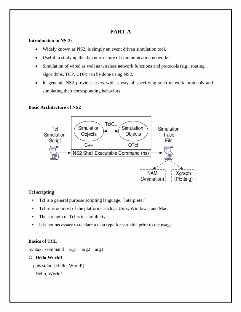
Introduction to NS-2:
Widely known as NS2, is simply an event driven simulation tool.
Useful in studying the dynamic nature of communication networks.
Simulation of wired as well as wireless network functions and protocols (e.g., routing
algorithms, TCP, UDP) can be done using NS2.
In general, NS2 provides users with a way of specifying such network protocols and
simulating their corresponding behaviors.
Basic Architecture of NS2
Tcl scripting
• Tcl is a general purpose scripting language. [Interpreter]
• Tcl runs on most of the platforms such as Unix, Windows, and Mac.
• The strength of Tcl is its simplicity.
• It is not necessary to declare a data type for variable prior to the usage.
Basics of TCL
Syntax: command arg1 arg2 arg3
Hello World!
puts stdout{Hello, World!}
Hello, World!
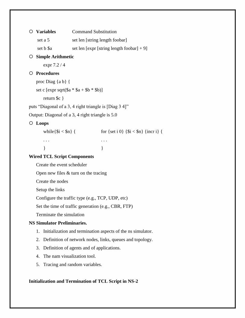
Variables Command Substitution
set a 5 set len [string length foobar]
set b $a set len [expr [string length foobar] + 9]
Simple Arithmetic
expr 7.2 / 4
Procedures
proc Diag {a b} {
set c [expr sqrt($a * $a + $b * $b)]
return $c }
puts ―Diagonal of a 3, 4 right triangle is [Diag 3 4]‖
Output: Diagonal of a 3, 4 right triangle is 5.0
Loops
while{$i < $n} { for {set i 0} {$i < $n} {incr i} {
. . . . . .
} }
Wired TCL Script Components
Create the event scheduler
Open new files & turn on the tracing
Create the nodes
Setup the links
Configure the traffic type (e.g., TCP, UDP, etc)
Set the time of traffic generation (e.g., CBR, FTP)
Terminate the simulation
NS Simulator Preliminaries.
1. Initialization and termination aspects of the ns simulator.
2. Definition of network nodes, links, queues and topology.
3. Definition of agents and of applications.
4. The nam visualization tool.
5. Tracing and random variables.
Initialization and Termination of TCL Script in NS-2

An ns simulation starts with the command
Which is thus the first line in the tcl script? This line declares a new variable as using the set
command, you can call this variable as you wish, In general people declares it as ns because it is
an instance of the Simulator class, so an object the code[new Simulator] is indeed the installation
of the class Simulator using the reserved word new.
In order to have output files with data on the simulation (trace files) or files used for
visualization (nam files), we need to create the files using ―open‖ command:
#Open the Trace file
#Open the NAM trace file
The above creates a dta trace file called ―out.tr‖ and a nam visualization trace file called
―out.nam‖.Within the tcl script,these files are not called explicitly by their names,but instead by
pointers that are declared above and called ―tracefile1‖ and ―namfile‖ respectively.Remark that
they begins with a # symbol.The second line open the file ―out.tr‖ to be used for writing,declared
with the letter ―w‖.The third line uses a simulator method called trace-all that have as parameter
the name of the file where the traces will go.
The last line tells the simulator to record all simulation traces in NAM input format.It
also gives the file name that the trace will be written to later by the command $ns flush-trace.In
our case,this will be the file pointed at by the pointer ―$namfile‖,i.e the file ―out.tr‖.
The termination of the program is done using a ―finish‖ procedure.
#Define a „finish‟ procedure
set ns [new Simulator]
set tracefile1 [open out.tr w]
$ns trace-all $tracefile1
set namfile [open out.nam w]
$ns namtrace-all $namfile

The word proc declares a procedure in this case called finish and without arguments. The
word global is used to tell that we are using variables declared outside the procedure. The
simulator method ―flush-trace” will dump the traces on the respective files. The tcl command
―close” closes the trace files defined before and exec executes the nam program for visualization.
The command exit will ends the application and return the number 0 as status to the system. Zero
is the default for a clean exit. Other values can be used to say that is a exit because something
fails.
At the end of ns program we should call the procedure ―finish‖ and specify at what time
the termination should occur. For example,
will be used to call ―finish‖ at time 125sec.Indeed,the at method of the simulator allows us to
schedule events explicitly.
The simulation can then begin using the command
Definition of a network of links and nodes
The way to define a node is
Proc finish { } {
global ns tracefile1 namfile
$ns flush-trace
Close $tracefile1
Close $namfile
Exec nam out.nam &
Exit 0
}
$ns at 125.0 “finish”
$ns run
set n0 [$ns node]
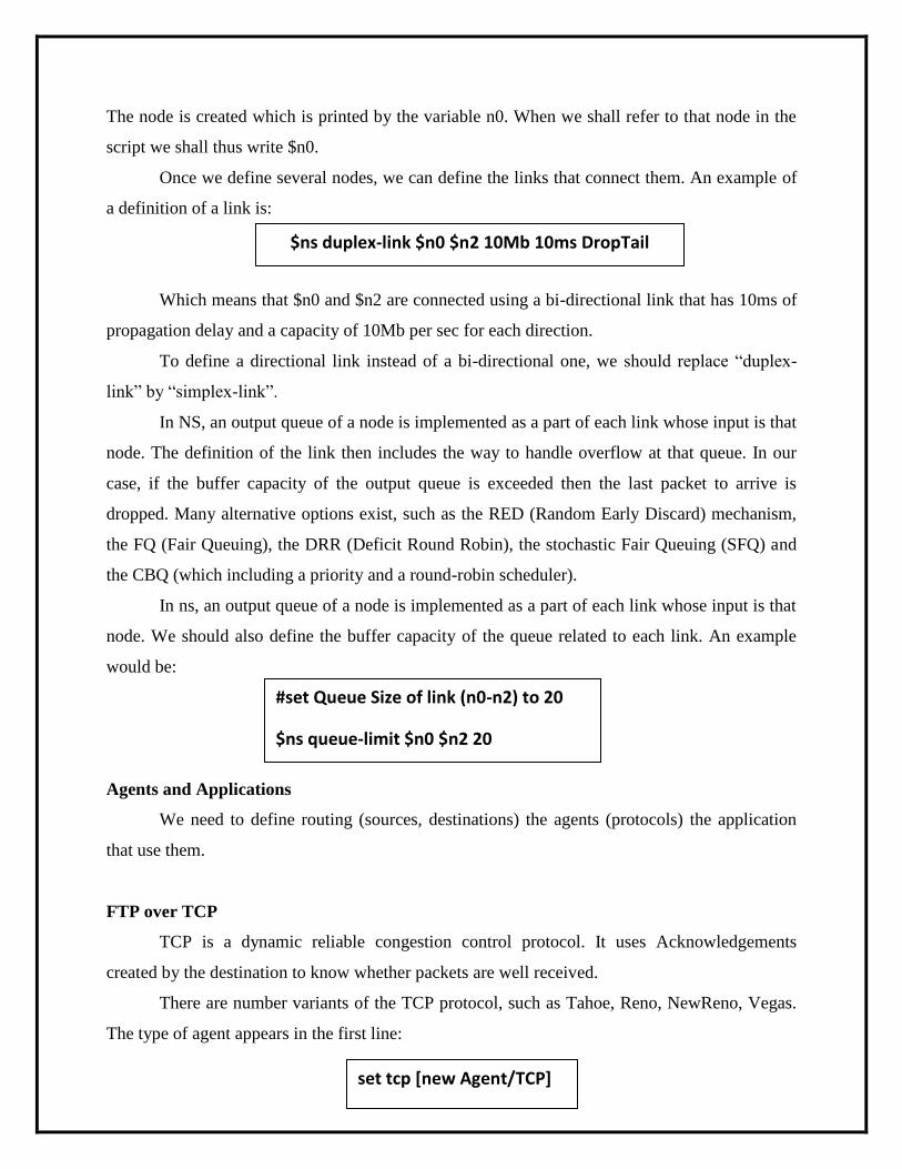
The node is created which is printed by the variable n0. When we shall refer to that node in the
script we shall thus write $n0.
Once we define several nodes, we can define the links that connect them. An example of
a definition of a link is:
Which means that $n0 and $n2 are connected using a bi-directional link that has 10ms of
propagation delay and a capacity of 10Mb per sec for each direction.
To define a directional link instead of a bi-directional one, we should replace ―duplex-
link‖ by ―simplex-link‖.
In NS, an output queue of a node is implemented as a part of each link whose input is that
node. The definition of the link then includes the way to handle overflow at that queue. In our
case, if the buffer capacity of the output queue is exceeded then the last packet to arrive is
dropped. Many alternative options exist, such as the RED (Random Early Discard) mechanism,
the FQ (Fair Queuing), the DRR (Deficit Round Robin), the stochastic Fair Queuing (SFQ) and
the CBQ (which including a priority and a round-robin scheduler).
In ns, an output queue of a node is implemented as a part of each link whose input is that
node. We should also define the buffer capacity of the queue related to each link. An example
would be:
Agents and Applications
We need to define routing (sources, destinations) the agents (protocols) the application
that use them.
FTP over TCP
TCP is a dynamic reliable congestion control protocol. It uses Acknowledgements
created by the destination to know whether packets are well received.
There are number variants of the TCP protocol, such as Tahoe, Reno, NewReno, Vegas.
The type of agent appears in the first line:
#set Queue Size of link (n0-n2) to 20
$ns queue-limit $n0 $n2 20
set tcp [new Agent/TCP]
$ns duplex-link $n0 $n2 10Mb 10ms DropTail
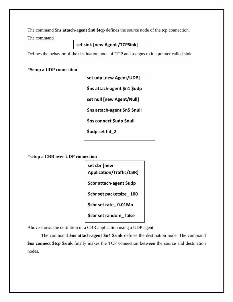
The command $ns attach-agent $n0 $tcp defines the source node of the tcp connection.
The command
Defines the behavior of the destination node of TCP and assigns to it a pointer called sink.
#Setup a UDP connection
#setup a CBR over UDP connection
Above shows the definition of a CBR application using a UDP agent
The command $ns attach-agent $n4 $sink defines the destination node. The command
$ns connect $tcp $sink finally makes the TCP connection between the source and destination
nodes.
set sink [new Agent /TCPSink]
set udp [new Agent/UDP]
$ns attach-agent $n1 $udp
set null [new Agent/Null]
$ns attach-agent $n5 $null
$ns connect $udp $null
$udp set fid_2
set cbr [new
Application/Traffic/CBR]
$cbr attach-agent $udp
$cbr set packetsize_ 100
$cbr set rate_ 0.01Mb
$cbr set random_ false
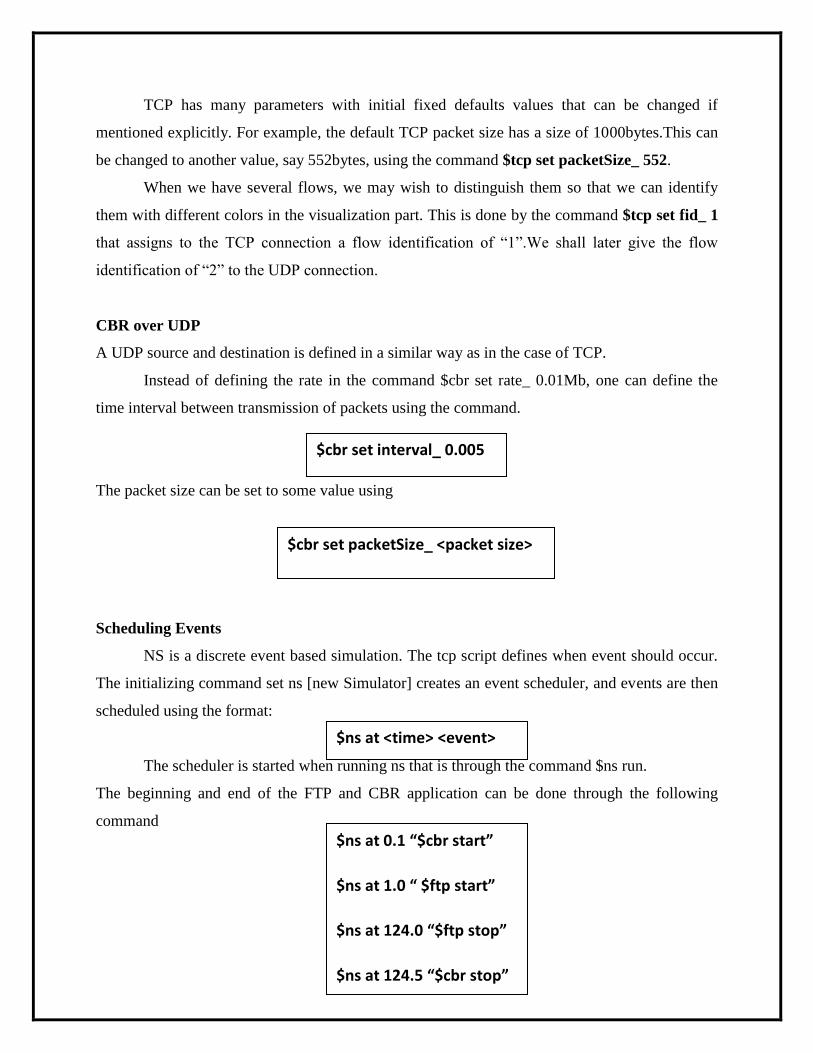
TCP has many parameters with initial fixed defaults values that can be changed if
mentioned explicitly. For example, the default TCP packet size has a size of 1000bytes.This can
be changed to another value, say 552bytes, using the command $tcp set packetSize_ 552.
When we have several flows, we may wish to distinguish them so that we can identify
them with different colors in the visualization part. This is done by the command $tcp set fid_ 1
that assigns to the TCP connection a flow identification of ―1‖.We shall later give the flow
identification of ―2‖ to the UDP connection.
CBR over UDP
A UDP source and destination is defined in a similar way as in the case of TCP.
Instead of defining the rate in the command $cbr set rate_ 0.01Mb, one can define the
time interval between transmission of packets using the command.
The packet size can be set to some value using
Scheduling Events
NS is a discrete event based simulation. The tcp script defines when event should occur.
The initializing command set ns [new Simulator] creates an event scheduler, and events are then
scheduled using the format:
The scheduler is started when running ns that is through the command $ns run.
The beginning and end of the FTP and CBR application can be done through the following
command
$cbr set interval_ 0.005
$cbr set packetSize_ <packet size>
$ns at <time> <event>
$ns at 0.1 “$cbr start”
$ns at 1.0 “ $ftp start”
$ns at 124.0 “$ftp stop”
$ns at 124.5 “$cbr stop”
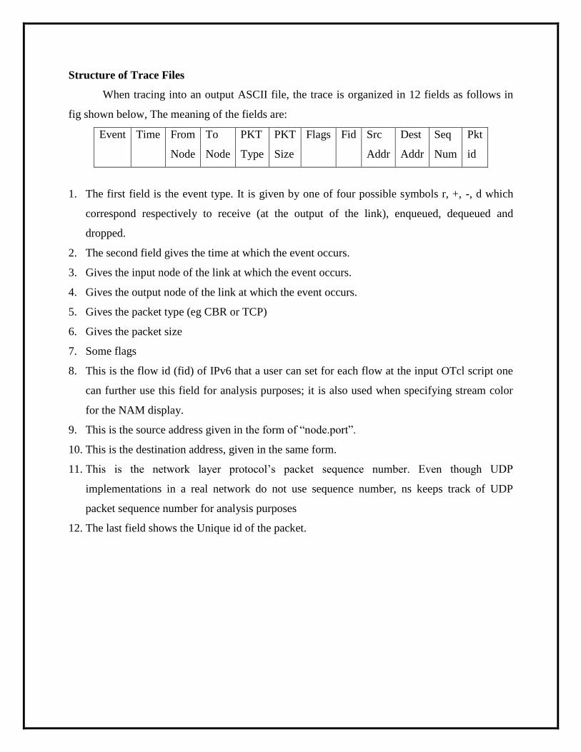
Structure of Trace Files
When tracing into an output ASCII file, the trace is organized in 12 fields as follows in
fig shown below, The meaning of the fields are:
Event Time From
Node
To
Node
PKT
Type
PKT
Size
Flags Fid Src
Addr
Dest
Addr
Seq
Num
Pkt
id
1. The first field is the event type. It is given by one of four possible symbols r, +, -, d which
correspond respectively to receive (at the output of the link), enqueued, dequeued and
dropped.
2. The second field gives the time at which the event occurs.
3. Gives the input node of the link at which the event occurs.
4. Gives the output node of the link at which the event occurs.
5. Gives the packet type (eg CBR or TCP)
6. Gives the packet size
7. Some flags
8. This is the flow id (fid) of IPv6 that a user can set for each flow at the input OTcl script one
can further use this field for analysis purposes; it is also used when specifying stream color
for the NAM display.
9. This is the source address given in the form of ―node.port‖.
10. This is the destination address, given in the same form.
11. This is the network layer protocol’s packet sequence number. Even though UDP
implementations in a real network do not use sequence number, ns keeps track of UDP
packet sequence number for analysis purposes
12. The last field shows the Unique id of the packet.
XGRAPH
The xgraph program draws a graph on an x-display given data read from either data file
or from standard input if no files are specified. It can display upto 64 independent data sets using
different colors and line styles for each set. It annotates the graph with a title, axis labels, grid
lines or tick marks, grid labels and a legend.
Syntax:
Options are listed here
/-bd <color> (Border)
This specifies the border color of the xgraph window.
/-bg <color> (Background)
This specifies the background color of the xgraph window.
/-fg<color> (Foreground)
This specifies the foreground color of the xgraph window.
/-lf <fontname> (LabelFont)
All axis labels and grid labels are drawn using this font.
/-t<string> (Title Text)
This string is centered at the top of the graph.
/-x <unit name> (XunitText)
This is the unit name for the x-axis. Its default is ―X‖.
/-y <unit name> (YunitText)
This is the unit name for the y-axis. Its default is ―Y‖.
Xgraph [options] file-name
Awk- An Advanced
awk is a programmable, pattern-matching, and processing tool available in UNIX. It
works equally well with text and numbers.
awk is not just a command, but a programming language too. In other words, awk utility
is a pattern scanning and processing language. It searches one or more files to see if they contain
lines that match specified patterns and then perform associated actions, such as writing the line to
the standard output or incrementing a counter each time it finds a match.
Syntax:
Here, selection_criteria filters input and select lines for the action component to act upon.
The selection_criteria is enclosed within single quotes and the action within the curly braces.
Both the selection_criteria and action forms an awk program.
Example: $ awk „/manager/ {print}‟ emp.lst
Variables
Awk allows the user to use variables of there choice. You can now print a serial number,
using the variable kount, and apply it those directors drawing a salary exceeding 6700:
$ awk –F”|” „$3 == “director” && $6 > 6700 {
kount =kount+1
printf “ %3f %20s %-12s %d\n”, kount,$2,$3,$6 }‟ empn.lst
THE –f OPTION: STORING awk PROGRAMS IN A FILE
You should holds large awk programs in separate file and provide them with the awk
extension for easier identification. Let’s first store the previous program in the file empawk.awk:
$ cat empawk.awk
Observe that this time we haven’t used quotes to enclose the awk program. You can now
use awk with the –f filename option to obtain the same output:
awk option ‘selection_criteria {action}’ file(s)
Awk –F”|” –f empawk.awk empn.lst

THE BEGIN AND END SECTIONS
Awk statements are usually applied to all lines selected by the address, and if there are no
addresses, then they are applied to every line of input. But, if you have to print something before
processing the first line, for example, a heading, then the BEGIN section can be used gainfully.
Similarly, the end section useful in printing some totals after processing is over.
The BEGIN and END sections are optional and take the form
BEGIN {action}
END {action}
These two sections, when present, are delimited by the body of the awk program. You
can use them to print a suitable heading at the beginning and the average salary at the end.
BUILT-IN VARIABLES
Awk has several built-in variables. They are all assigned automatically, though it is also
possible for a user to reassign some of them. You have already used NR, which signifies the
record number of the current line. We’ll now have a brief look at some of the other variable.
The FS Variable: as stated elsewhere, awk uses a contiguous string of spaces as the default field
delimiter. FS redefines this field separator, which in the sample database happens to be the |.
When used at all, it must occur in the BEGIN section so that the body of the program knows its
value before it starts processing:
BEGIN {FS=”|”}
This is an alternative to the –F option which does the same thing.
The OFS Variable: when you used the print statement with comma-separated arguments, each
argument was separated from the other by a space. This is awk’s default output field separator,
and can reassigned using the variable OFS in the BEGIN section:
BEGIN { OFS=”~” }
When you reassign this variable with a ~ (tilde), awk will use this character for delimiting the
print arguments. This is a useful variable for creating lines with delimited fields.
The NF variable: NF comes in quite handy for cleaning up a database of lines that don’t contain
the right number of fields. By using it on a file, say emp.lst, you can locate those lines not having
6 fields, and which have crept in due to faulty data entry:
$awk „BEGIN {FS = “|”}
NF! =6 { Print “Record No “, NR, “has”, “fields”}‟ empx.lst
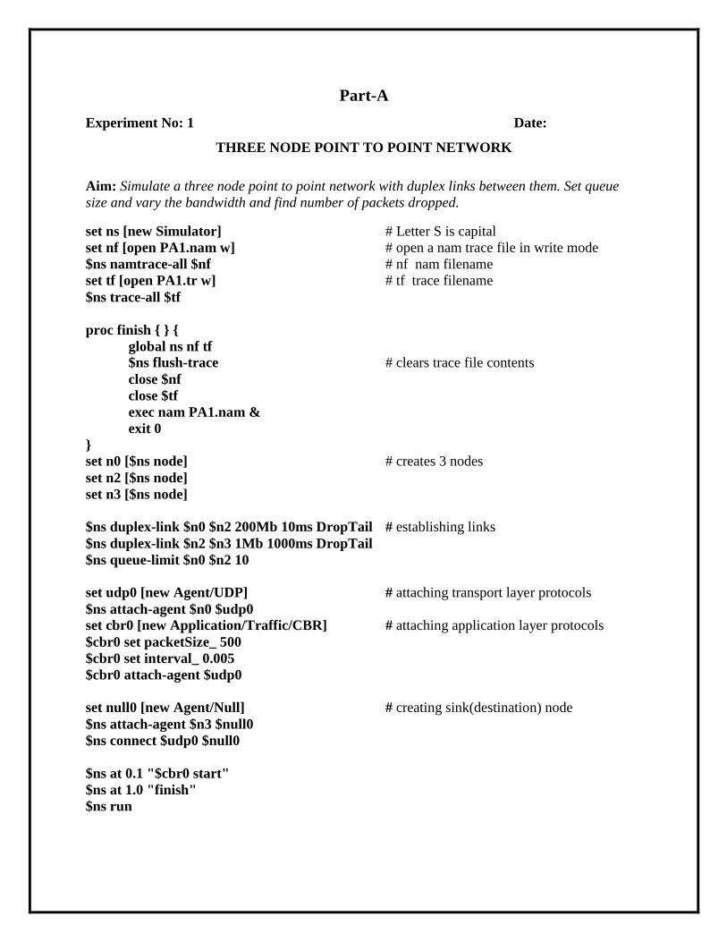
Part-A
Experiment No: 1 Date:
THREE NODE POINT TO POINT NETWORK
Aim: Simulate a three node point to point network with duplex links between them. Set queue
size and vary the bandwidth and find number of packets dropped.
set ns [new Simulator] # Letter S is capital
set nf [open PA1.nam w] # open a nam trace file in write mode
$ns namtrace-all $nf # nf nam filename
set tf [open PA1.tr w] # tf trace filename
$ns trace-all $tf
proc finish { } {
global ns nf tf
$ns flush-trace # clears trace file contents
close $nf
close $tf
exec nam PA1.nam &
exit 0
}
set n0 [$ns node] # creates 3 nodes
set n2 [$ns node]
set n3 [$ns node]
$ns duplex-link $n0 $n2 200Mb 10ms DropTail # establishing links
$ns duplex-link $n2 $n3 1Mb 1000ms DropTail
$ns queue-limit $n0 $n2 10
set udp0 [new Agent/UDP] # attaching transport layer protocols
$ns attach-agent $n0 $udp0
set cbr0 [new Application/Traffic/CBR] # attaching application layer protocols
$cbr0 set packetSize_ 500
$cbr0 set interval_ 0.005
$cbr0 attach-agent $udp0
set null0 [new Agent/Null] # creating sink(destination) node
$ns attach-agent $n3 $null0
$ns connect $udp0 $null0
$ns at 0.1 "$cbr0 start"
$ns at 1.0 "finish"
$ns run
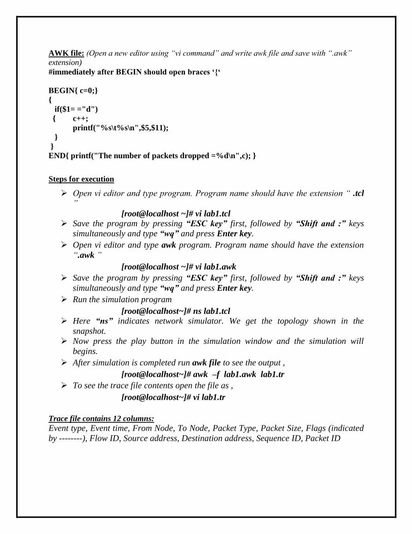
AWK file: (Open a new editor using “vi command” and write awk file and save with “.awk”
extension)
#immediately after BEGIN should open braces „{„
BEGIN{ c=0;}
{
if($1= ="d")
{ c++;
printf("%s\t%s\n",$5,$11);
}
}
END{ printf("The number of packets dropped =%d\n",c); }
Steps for execution
Open vi editor and type program. Program name should have the extension “ .tcl
”
[root@localhost ~]# vi lab1.tcl
Save the program by pressing “ESC key” first, followed by “Shift and :” keys
simultaneously and type “wq” and press Enter key.
Open vi editor and type awk program. Program name should have the extension
“.awk ”
[root@localhost ~]# vi lab1.awk
Save the program by pressing “ESC key” first, followed by “Shift and :” keys
simultaneously and type “wq” and press Enter key.
Run the simulation program
[root@localhost~]# ns lab1.tcl
Here “ns” indicates network simulator. We get the topology shown in the
snapshot.
Now press the play button in the simulation window and the simulation will
begins.
After simulation is completed run awk file to see the output ,
[root@localhost~]# awk –f lab1.awk lab1.tr
To see the trace file contents open the file as ,
[root@localhost~]# vi lab1.tr
Trace file contains 12 columns:
Event type, Event time, From Node, To Node, Packet Type, Packet Size, Flags (indicated
by --------), Flow ID, Source address, Destination address, Sequence ID, Packet ID
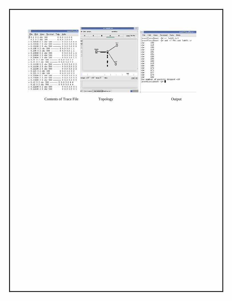
Contents of Trace File Topology Output
Experiment No: 2 Date:
FOUR NODE POINT TO POINT NETWORK
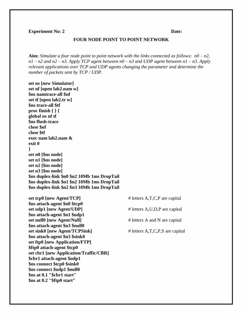
Aim: Simulate a four node point to point network with the links connected as follows: n0 – n2,
n1 – n2 and n2 – n3. Apply TCP agent between n0 – n3 and UDP agent between n1 – n3. Apply
relevant applications over TCP and UDP agents changing the parameter and determine the
number of packets sent by TCP / UDP.
set ns [new Simulator]
set nf [open lab2.nam w]
$ns namtrace-all $nf
set tf [open lab2.tr w]
$ns trace-all $tf
proc finish { } {
global ns nf tf
$ns flush-trace
close $nf
close $tf
exec nam lab2.nam &
exit 0
}
set n0 [$ns node]
set n1 [$ns node]
set n2 [$ns node]
set n3 [$ns node]
$ns duplex-link $n0 $n2 10Mb 1ms DropTail
$ns duplex-link $n1 $n2 10Mb 1ms DropTail
$ns duplex-link $n2 $n3 10Mb 1ms DropTail
set tcp0 [new Agent/TCP] # letters A,T,C,P are capital
$ns attach-agent $n0 $tcp0
set udp1 [new Agent/UDP] # letters A,U,D,P are capital
$ns attach-agent $n1 $udp1
set null0 [new Agent/Null] # letters A and N are capital
$ns attach-agent $n3 $null0
set sink0 [new Agent/TCPSink] # letters A,T,C,P,S are capital
$ns attach-agent $n3 $sink0
set ftp0 [new Application/FTP]
$ftp0 attach-agent $tcp0
set cbr1 [new Application/Traffic/CBR]
$cbr1 attach-agent $udp1
$ns connect $tcp0 $sink0
$ns connect $udp1 $null0
$ns at 0.1 "$cbr1 start"
$ns at 0.2 "$ftp0 start"
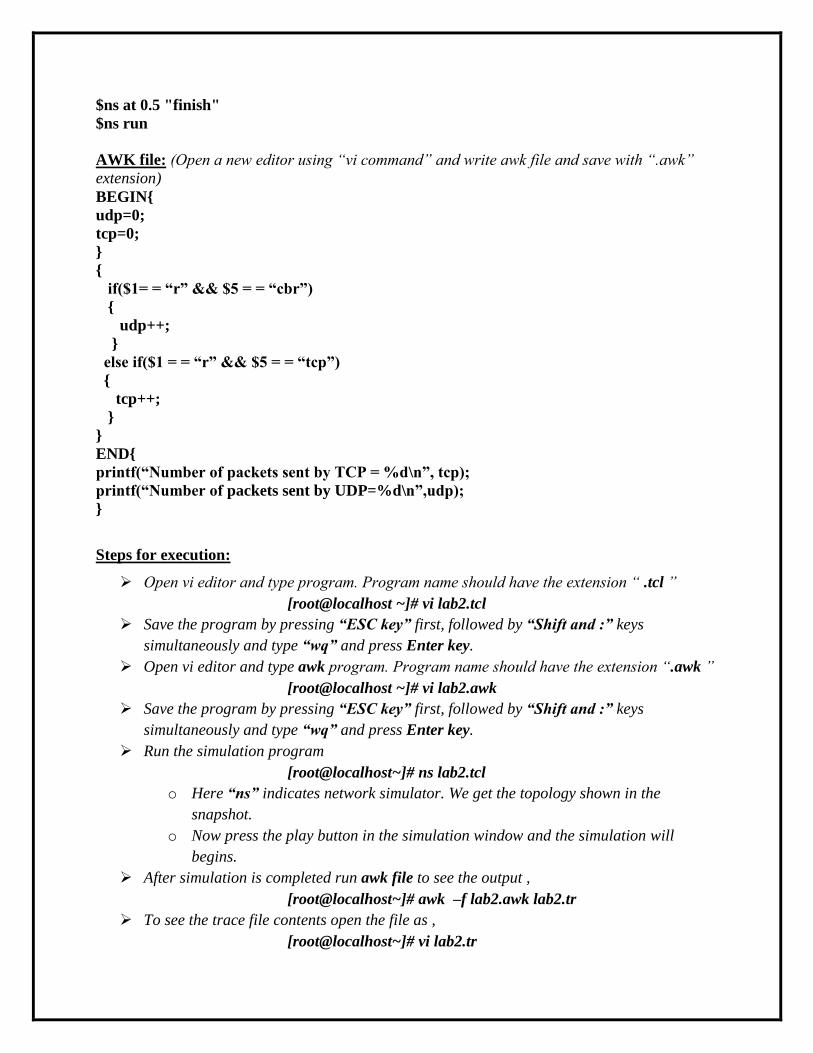
$ns at 0.5 "finish"
$ns run
AWK file: (Open a new editor using “vi command” and write awk file and save with “.awk”
extension)
BEGIN{
udp=0;
tcp=0;
}
{
if($1= = “r” && $5 = = “cbr”)
{
udp++;
}
else if($1 = = “r” && $5 = = “tcp”)
{
tcp++;
}
}
END{
printf(“Number of packets sent by TCP = %d\n”, tcp);
printf(“Number of packets sent by UDP=%d\n”,udp);
}
Steps for execution:
Open vi editor and type program. Program name should have the extension “ .tcl ”
[root@localhost ~]# vi lab2.tcl
Save the program by pressing “ESC key” first, followed by “Shift and :” keys
simultaneously and type “wq” and press Enter key.
Open vi editor and type awk program. Program name should have the extension “.awk ”
[root@localhost ~]# vi lab2.awk
Save the program by pressing “ESC key” first, followed by “Shift and :” keys
simultaneously and type “wq” and press Enter key.
Run the simulation program
[root@localhost~]# ns lab2.tcl
o Here “ns” indicates network simulator. We get the topology shown in the
snapshot.
o Now press the play button in the simulation window and the simulation will
begins.
After simulation is completed run awk file to see the output ,
[root@localhost~]# awk –f lab2.awk lab2.tr
To see the trace file contents open the file as ,
[root@localhost~]# vi lab2.tr
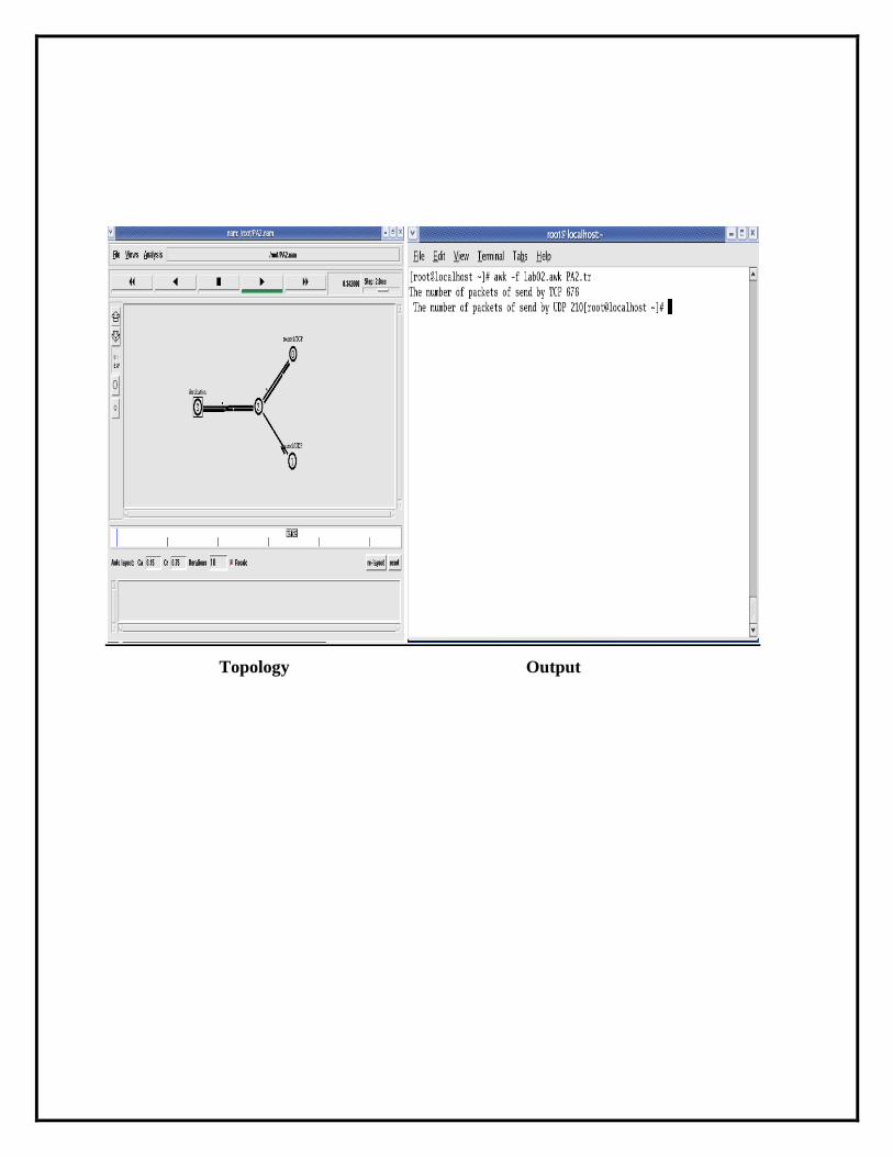
Topology Output

Experiment No: 3 Date:
TRANSMISSION OF PING MESSAGE
Aim: Simulate the transmission of ping messages over a network topology consisting of 6 nodes
and find the number of packets dropped due to congestion.
set ns [ new Simulator ]
set nf [ open lab4.nam w ]
$ns namtrace-all $nf
set tf [ open lab4.tr w ]
$ns trace-all $tf
set n0 [$ns node]
set n1 [$ns node]
set n2 [$ns node]
set n3 [$ns node]
set n4 [$ns node]
set n5 [$ns node]
$ns duplex-link $n0 $n4 1005Mb 1ms DropTail
$ns duplex-link $n1 $n4 50Mb 1ms DropTail
$ns duplex-link $n2 $n4 2000Mb 1ms DropTail
$ns duplex-link $n3 $n4 200Mb 1ms DropTail
$ns duplex-link $n4 $n5 1Mb 1ms DropTail
set p1 [new Agent/Ping] # letters A and P should be capital
$ns attach-agent $n0 $p1
$p1 set packetSize_ 50000
$p1 set interval_ 0.0001
set p2 [new Agent/Ping] # letters A and P should be capital
$ns attach-agent $n1 $p2
set p3 [new Agent/Ping] # letters A and P should be capital
$ns attach-agent $n2 $p3
$p3 set packetSize_ 30000
$p3 set interval_ 0.00001
set p4 [new Agent/Ping] # letters A and P should be capital
$ns attach-agent $n3 $p4
set p5 [new Agent/Ping] # letters A and P should be capital
$ns attach-agent $n5 $p5
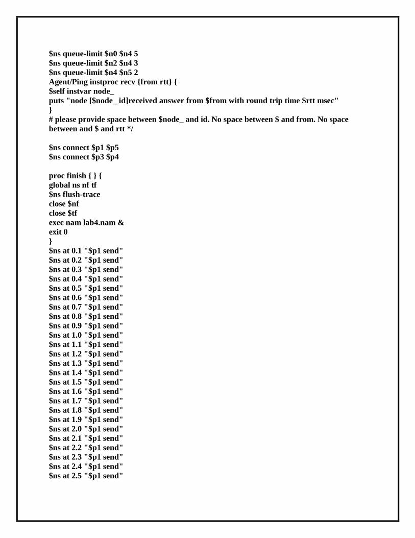
$ns queue-limit $n0 $n4 5
$ns queue-limit $n2 $n4 3
$ns queue-limit $n4 $n5 2
Agent/Ping instproc recv {from rtt} {
$self instvar node_
puts "node [$node_ id]received answer from $from with round trip time $rtt msec"
}
# please provide space between $node_ and id. No space between $ and from. No space
between and $ and rtt */
$ns connect $p1 $p5
$ns connect $p3 $p4
proc finish { } {
global ns nf tf
$ns flush-trace
close $nf
close $tf
exec nam lab4.nam &
exit 0
}
$ns at 0.1 "$p1 send"
$ns at 0.2 "$p1 send"
$ns at 0.3 "$p1 send"
$ns at 0.4 "$p1 send"
$ns at 0.5 "$p1 send"
$ns at 0.6 "$p1 send"
$ns at 0.7 "$p1 send"
$ns at 0.8 "$p1 send"
$ns at 0.9 "$p1 send"
$ns at 1.0 "$p1 send"
$ns at 1.1 "$p1 send"
$ns at 1.2 "$p1 send"
$ns at 1.3 "$p1 send"
$ns at 1.4 "$p1 send"
$ns at 1.5 "$p1 send"
$ns at 1.6 "$p1 send"
$ns at 1.7 "$p1 send"
$ns at 1.8 "$p1 send"
$ns at 1.9 "$p1 send"
$ns at 2.0 "$p1 send"
$ns at 2.1 "$p1 send"
$ns at 2.2 "$p1 send"
$ns at 2.3 "$p1 send"
$ns at 2.4 "$p1 send"
$ns at 2.5 "$p1 send"

$ns at 2.6 "$p1 send"
$ns at 2.7 "$p1 send"
$ns at 2.8 "$p1 send"
$ns at 2.9 "$p1 send"
$ns at 0.1 "$p3 send"
$ns at 0.2 "$p3 send"
$ns at 0.3 "$p3 send"
$ns at 0.4 "$p3 send"
$ns at 0.5 "$p3 send"
$ns at 0.6 "$p3 send"
$ns at 0.7 "$p3 send"
$ns at 0.8 "$p3 send"
$ns at 0.9 "$p3 send"
$ns at 1.0 "$p3 send"
$ns at 1.1 "$p3 send"
$ns at 1.2 "$p3 send"
$ns at 1.3 "$p3 send"
$ns at 1.4 "$p3 send"
$ns at 1.5 "$p3 send"
$ns at 1.6 "$p3 send"
$ns at 1.7 "$p3 send"
$ns at 1.8 "$p3 send"
$ns at 1.9 "$p3 send"
$ns at 2.0 "$p3 send"
$ns at 2.1 "$p3 send"
$ns at 2.2 "$p3 send"
$ns at 2.3 "$p3 send"
$ns at 2.4 "$p3 send"
$ns at 2.5 "$p3 send"
$ns at 2.6 "$p3 send"
$ns at 2.7 "$p3 send"
$ns at 2.8 "$p3 send"
$ns at 2.9 "$p3 send"
$ns at 3.0 "finish"
$ns run
AWK file: (Open a new editor using “vi command” and write awk file and save with “.awk”
extension)
BEGIN{
drop=0;
}
{
if($1= ="d" )
{
drop++;
}
}
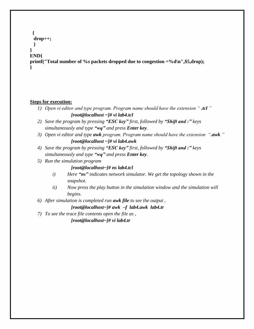
END{
printf("Total number of %s packets dropped due to congestion =%d\n",$5,drop);
}
Steps for execution:
1) Open vi editor and type program. Program name should have the extension “ .tcl ”
[root@localhost ~]# vi lab4.tcl
2) Save the program by pressing “ESC key” first, followed by “Shift and :” keys
simultaneously and type “wq” and press Enter key.
3) Open vi editor and type awk program. Program name should have the extension “.awk ”
[root@localhost ~]# vi lab4.awk
4) Save the program by pressing “ESC key” first, followed by “Shift and :” keys
simultaneously and type “wq” and press Enter key.
5) Run the simulation program
[root@localhost~]# ns lab4.tcl
i) Here “ns” indicates network simulator. We get the topology shown in the
snapshot.
ii) Now press the play button in the simulation window and the simulation will
begins.
6) After simulation is completed run awk file to see the output ,
[root@localhost~]# awk –f lab4.awk lab4.tr
7) To see the trace file contents open the file as ,
[root@localhost~]# vi lab4.tr
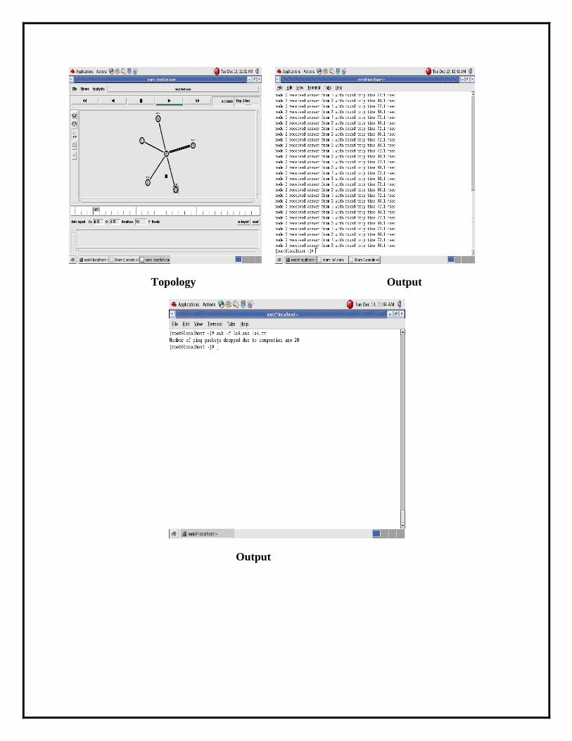
Topology Output
Output

Experiment No: 4 Date:
ETHERNET LAN USING N-NODES
Aim: Simulate an Ethernet LAN using „n‟ nodes, change error rate and data rate and compare
throughput.
set ns [new Simulator]
set tf [open lab5.tr w]
$ns trace-all $tf
set nf [open lab5.nam w]
$ns namtrace-all $nf
$ns color 0 blue
set n0 [$ns node]
$n0 color "red"
set n1 [$ns node]
$n1 color "red"
set n2 [$ns node]
$n2 color "red"
set n3 [$ns node]
$n3 color "red"
set n4 [$ns node]
$n4 color "magenta"
set n5 [$ns node]
$n5 color "magenta"
set n6 [$ns node]
$n6 color "magenta"
set n7 [$ns node]
$n7 color "magenta"
$ns make-lan "$n0 $n1 $n2 $n3" 100Mb 300ms LL Queue/ DropTail Mac/802_3
$ns make-lan "$n4 $n5 $n6 $n7" 100Mb 300ms LL Queue/ DropTail Mac/802_3
$ns duplex-link $n3 $n4 100Mb 300ms DropTail
$ns duplex-link-op $n3 $n4 color "green"
# set error rate. Here ErrorModel is a class and it is single word and space should not be
given between Error and Model
# lossmodel is a command and it is single word. Space should not be given between loss and
model
set err [new ErrorModel]
$ns lossmodel $err $n3 $n4
$err set rate_ 0.1
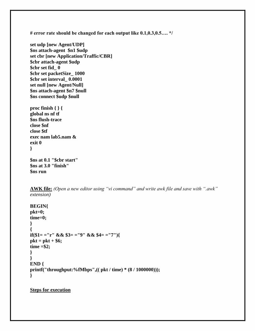
# error rate should be changed for each output like 0.1,0.3,0.5…. */
set udp [new Agent/UDP]
$ns attach-agent $n1 $udp
set cbr [new Application/Traffic/CBR]
$cbr attach-agent $udp
$cbr set fid_ 0
$cbr set packetSize_ 1000
$cbr set interval_ 0.0001
set null [new Agent/Null]
$ns attach-agent $n7 $null
$ns connect $udp $null
proc finish { } {
global ns nf tf
$ns flush-trace
close $nf
close $tf
exec nam lab5.nam &
exit 0
}
$ns at 0.1 "$cbr start"
$ns at 3.0 "finish"
$ns run
AWK file: (Open a new editor using “vi command” and write awk file and save with “.awk”
extension)
BEGIN{
pkt=0;
time=0;
}
{
if($1= ="r" && $3= ="9" && $4= ="7"){
pkt = pkt + $6;
time =$2;
}
}
END {
printf("throughput:%fMbps",(( pkt / time) * (8 / 1000000)));
}
Steps for execution
Open vi editor and type program. Program name should have the extension “ .tcl ”
[root@localhost ~]# vi lab5.tcl
Save the program by pressing “ESC key” first, followed by “Shift and :” keys
simultaneously and type “wq” and press Enter key.
Open vi editor and type awk program. Program name should have the extension “.awk ”
[root@localhost ~]# vi lab5.awk
Save the program by pressing “ESC key” first, followed by “Shift and :” keys
simultaneously and type “wq” and press Enter key.
Run the simulation program
[root@localhost~]# ns lab5.tcl
o Here “ns” indicates network simulator. We get the topology shown in the
snapshot.
o Now press the play button in the simulation window and the simulation will
begins.
After simulation is completed run awk file to see the output ,
[root@localhost~]# awk –f lab5.awk lab5.tr
To see the trace file contents open the file as ,
[root@localhost~]# vi lab5.tr
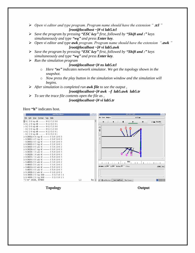
Here “h” indicates host.
Topology Output

This above output is for error rate 0.1. During next execution of simulation change error rate to
0.3, 0.5,….. and check its effect on throughput.
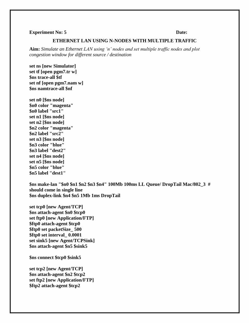
Experiment No: 5 Date:
ETHERNET LAN USING N-NODES WITH MULTIPLE TRAFFIC
Aim: Simulate an Ethernet LAN using „n‟ nodes and set multiple traffic nodes and plot
congestion window for different source / destination
set ns [new Simulator]
set tf [open pgm7.tr w]
$ns trace-all $tf
set nf [open pgm7.nam w]
$ns namtrace-all $nf
set n0 [$ns node]
$n0 color "magenta"
$n0 label "src1"
set n1 [$ns node]
set n2 [$ns node]
$n2 color "magenta"
$n2 label "src2"
set n3 [$ns node]
$n3 color "blue"
$n3 label "dest2"
set n4 [$ns node]
set n5 [$ns node]
$n5 color "blue"
$n5 label "dest1"
$ns make-lan "$n0 $n1 $n2 $n3 $n4" 100Mb 100ms LL Queue/ DropTail Mac/802_3 #
should come in single line
$ns duplex-link $n4 $n5 1Mb 1ms DropTail
set tcp0 [new Agent/TCP]
$ns attach-agent $n0 $tcp0
set ftp0 [new Application/FTP]
$ftp0 attach-agent $tcp0
$ftp0 set packetSize_ 500
$ftp0 set interval_ 0.0001
set sink5 [new Agent/TCPSink]
$ns attach-agent $n5 $sink5
$ns connect $tcp0 $sink5
set tcp2 [new Agent/TCP]
$ns attach-agent $n2 $tcp2
set ftp2 [new Application/FTP]
$ftp2 attach-agent $tcp2
$ftp2 set packetSize_ 600
$ftp2 set interval_ 0.001
set sink3 [new Agent/TCPSink]
$ns attach-agent $n3 $sink3
$ns connect $tcp2 $sink3
set file1 [open file1.tr w]
$tcp0 attach $file1
set file2 [open file2.tr w]
$tcp2 attach $file2
$tcp0 trace cwnd_ # must put underscore ( _ ) after cwnd and no space between them
$tcp2 trace cwnd_
proc finish { } {
global ns nf tf
$ns flush-trace
close $tf
close $nf
exec nam pgm7.nam &
exit 0
}
$ns at 0.1 "$ftp0 start"
$ns at 5 "$ftp0 stop"
$ns at 7 "$ftp0 start"
$ns at 0.2 "$ftp2 start"
$ns at 8 "$ftp2 stop"
$ns at 14 "$ftp0 stop"
$ns at 10 "$ftp2 start"
$ns at 15 "$ftp2 stop"
$ns at 16 "finish"
$ns run
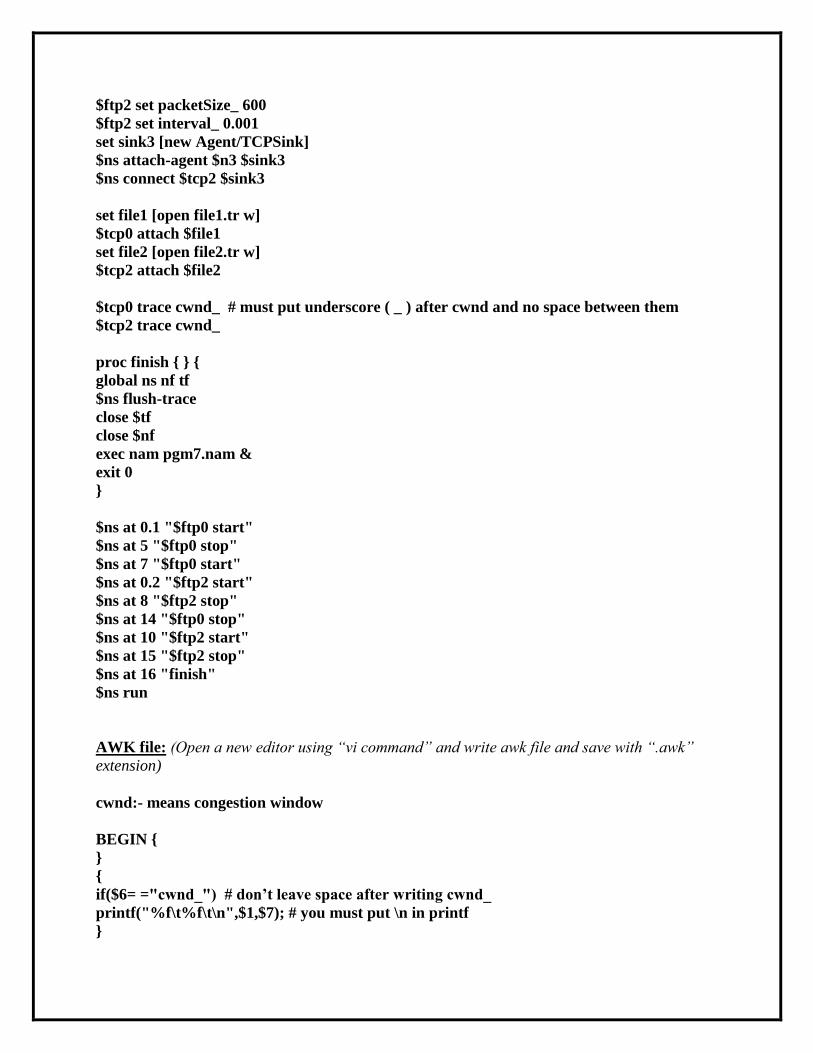
AWK file: (Open a new editor using “vi command” and write awk file and save with “.awk”
extension)
cwnd:- means congestion window
BEGIN {
}
{
if($6= ="cwnd_") # don‟t leave space after writing cwnd_
printf("%f\t%f\t\n",$1,$7); # you must put \n in printf
}
END {
}
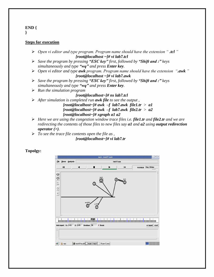
Steps for execution
Open vi editor and type program. Program name should have the extension “ .tcl ”
[root@localhost ~]# vi lab7.tcl
Save the program by pressing “ESC key” first, followed by “Shift and :” keys
simultaneously and type “wq” and press Enter key.
Open vi editor and type awk program. Program name should have the extension “.awk ”
[root@localhost ~]# vi lab7.awk
Save the program by pressing “ESC key” first, followed by “Shift and :” keys
simultaneously and type “wq” and press Enter key.
Run the simulation program
[root@localhost~]# ns lab7.tcl
After simulation is completed run awk file to see the output ,
[root@localhost~]# awk –f lab7.awk file1.tr > a1
[root@localhost~]# awk –f lab7.awk file2.tr > a2
[root@localhost~]# xgraph a1 a2
Here we are using the congestion window trace files i.e. file1.tr and file2.tr and we are
redirecting the contents of those files to new files say a1 and a2 using output redirection
operator (>).
To see the trace file contents open the file as ,
[root@localhost~]# vi lab7.tr
Topolgy:
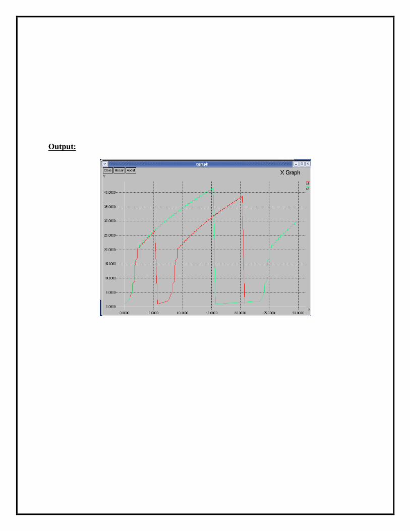
Output:
Experiment No: 6 Date:
SIMPLE ESS WITH WIRELESS LAN
Aim: Simulate simple ESS and with transmitting nodes in wireless LAN by simulation and
determine the performance with respect to transmission of packets.
set ns [new Simulator]
set tf [open lab8.tr w]
$ns trace-all $tf
set topo [new Topography]
$topo load_flatgrid 1000 1000
set nf [open lab8.nam w]
$ns namtrace-all-wireless $nf 1000 1000
$ns node-config -adhocRouting DSDV \
-llType LL \
-macType Mac/802_11 \
-ifqType Queue/DropTail \
-ifqLen 50 \
-phyType Phy/WirelessPhy \
-channelType Channel/WirelessChannel \
-prrootype Propagation/TwoRayGround \
-antType Antenna/OmniAntenna \
-topoInstance $topo \
-agentTrace ON \
-routerTrace ON
create-god 3
set n0 [$ns node]
set n1 [$ns node]
set n2 [$ns node]
$n0 label "tcp0"
$n1 label "sink1/tcp1"
$n2 label "sink2"
$n0 set X_ 50
$n0 set Y_ 50
$n0 set Z_ 0
$n1 set X_ 100
$n1 set Y_ 100
$n1 set Z_ 0
$n2 set X_ 600
$n2 set Y_ 600
$n2 set Z_ 0
$ns at 0.1 "$n0 setdest 50 50 15"
$ns at 0.1 "$n1 setdest 100 100 25"
$ns at 0.1 "$n2 setdest 600 600 25"
set tcp0 [new Agent/TCP]
$ns attach-agent $n0 $tcp0
set ftp0 [new Application/FTP]
$ftp0 attach-agent $tcp0
set sink1 [new Agent/TCPSink]
$ns attach-agent $n1 $sink1
$ns connect $tcp0 $sink1
set tcp1 [new Agent/TCP]
$ns attach-agent $n1 $tcp1
set ftp1 [new Application/FTP]
$ftp1 attach-agent $tcp1
set sink2 [new Agent/TCPSink]
$ns attach-agent $n2 $sink2
$ns connect $tcp1 $sink2
$ns at 5 "$ftp0 start"
$ns at 5 "$ftp1 start"
$ns at 100 "$n1 setdest 550 550 15"
$ns at 190 "$n1 setdest 70 70 15"
proc finish { } {
global ns nf tf
$ns flush-trace
exec nam lab8.nam &
close $tf
exit 0
}
$ns at 250 "finish"
$ns run
AWK file: (Open a new editor using “vi command” and write awk file and save with “.awk”
extension)
BEGIN{
count1=0
count2=0
pack1=0
pack2=0
time1=0
time2=0
}
{
if($1= ="r"&& $3= ="_1_" && $4= ="AGT")
{
count1++
pack1=pack1+$8
time1=$2
}
if($1= ="r" && $3= ="_2_" && $4= ="AGT")
{
count2++
pack2=pack2+$8
time2=$2
}
}
END{
printf("The Throughput from n0 to n1: %f Mbps \n‖, ((count1*pack1*8)/(time1*1000000)));
printf("The Throughput from n1 to n2: %f Mbps", ((count2*pack2*8)/(time2*1000000)));
}
Steps for execution
Open vi editor and type program. Program name should have the extension “ .tcl ”
[root@localhost ~]# vi lab8.tcl
Save the program by pressing “ESC key” first, followed by “Shift and :” keys
simultaneously and type “wq” and press Enter key.
Open vi editor and type awk program. Program name should have the extension “.awk ”
[root@localhost ~]# vi lab8.awk
Save the program by pressing “ESC key” first, followed by “Shift and :” keys
simultaneously and type “wq” and press Enter key.
Run the simulation program
[root@localhost~]# ns lab8.tcl
o Here “ns” indicates network simulator. We get the topology shown in the
snapshot.
o Now press the play button in the simulation window and the simulation will
begins.
After simulation is completed run awk file to see the output ,
[root@localhost~]# awk –f lab8.awk lab8.tr
To see the trace file contents open the file as ,
[root@localhost~]# vi lab8.tr
Output:
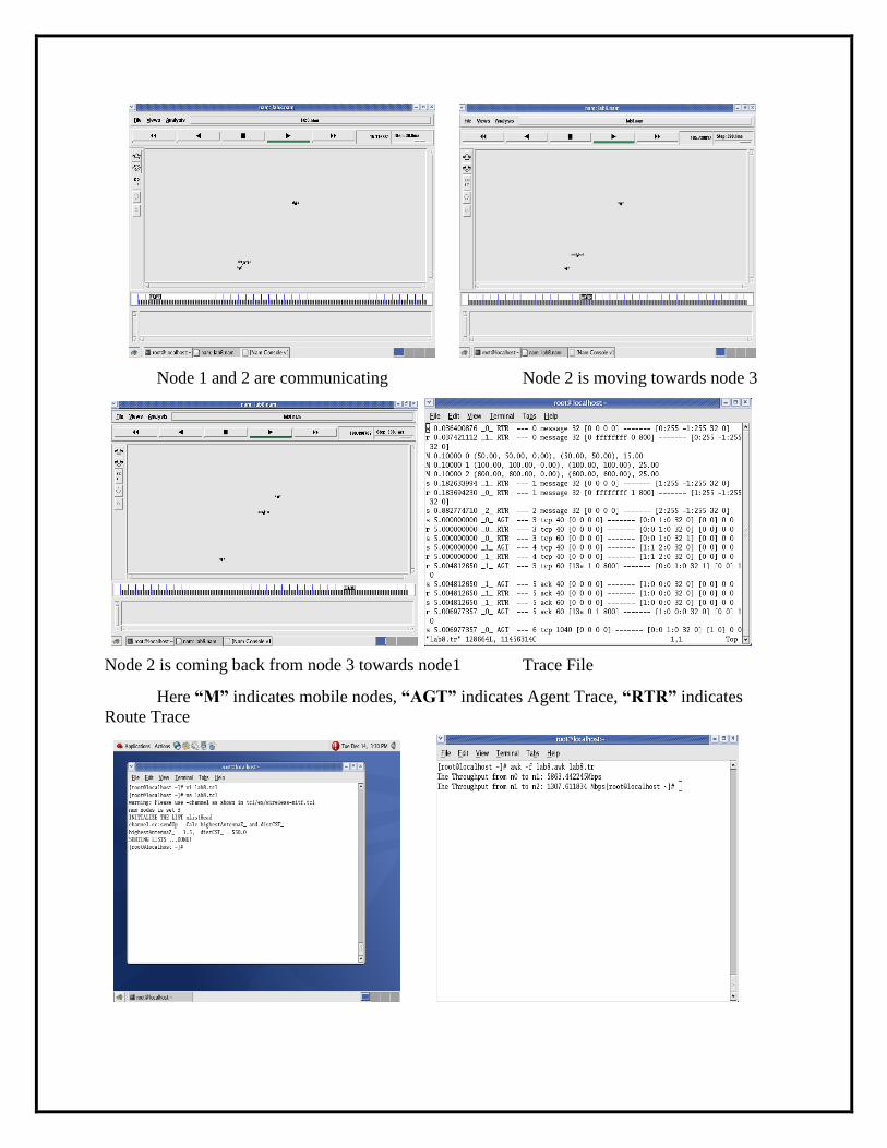
Node 1 and 2 are communicating Node 2 is moving towards node 3
Node 2 is coming back from node 3 towards node1 Trace File
Here “M” indicates mobile nodes, “AGT” indicates Agent Trace, “RTR” indicates
Route Trace

Part-B
Experiment No: 1 Date:
Error Detecting Code Using CRC-CCITT (16-bit)
Aim: C Program for ERROR detecting code using CRC-CCITT (16bit).
Whenever digital data is stored or interfaced, data corruption might occur. Since the
beginning of computer science, developers have been thinking of ways to deal with this type of
problem. For serial data they came up with the solution to attach a parity bit to each sent byte.
This simple detection mechanism works if an odd number of bits in a byte changes, but an even
number of false bits in one byte will not be detected by the parity check. To overcome this
problem developers have searched for mathematical sound mechanisms to detect multiple false
bits. The CRC calculation or cyclic redundancy check was the result of this. Nowadays CRC
calculations are used in all types of communications. All packets sent over a network connection
are checked with a CRC. Also each data block on your hard disk has a CRC value attached to it.
Modern computer world cannot do without these CRC calculations. So let's see why they are so
widely used. The answer is simple; they are powerful, detect many types of errors and are
extremely fast to calculate especially when dedicated hardware chips are used.
The idea behind CRC calculation is to look at the data as one large binary number. This
number is divided by a certain value and the remainder of the calculation is called the CRC.
Dividing in the CRC calculation at first looks to cost a lot of computing power, but it can be
performed very quickly if we use a method similar to the one learned at school. We will as an
example calculate the remainder for the character 'm'—which is 1101101 in binary notation—by
dividing it by 19 or 10011. Please note that 19 is an odd number. This is necessary as we will see
further on. Please refer to your schoolbooks as the binary calculation method here is not very
different from the decimal method you learned when you were young. It might only look a little
bit strange. Also notations differ between countries, but the method is similar.

With decimal calculations you can quickly check that 109 divided by 19 gives a quotient
of 5 with 14 as the remainder. But what we also see in the scheme is that every bit extra to check
only costs one binary comparison and in 50% of the cases one binary subtraction. You can easily
increase the number of bits of the test data string—for example to 56 bits if we use our example
value "Lammert"—and the result can be calculated with 56 binary comparisons and an average
of 28 binary subtractions. This can be implemented in hardware directly with only very few
transistors involved. Also software algorithms can be very efficient.
All of the CRC formulas you will encounter are simply checksum algorithms based on
modulo-2 binary division where we ignore carry bits and in effect the subtraction will be equal to
an exclusive or operation. Though some differences exist in the specifics across different CRC
formulas, the basic mathematical process is always the same:
The message bits are appended with c zero bits; this augmented message is the dividend
A predetermined c+1-bit binary sequence, called the generator polynomial, is the divisor
The checksum is the c-bit remainder that results from the division operation
Table 1 lists some of the most commonly used generator polynomials for 16- and 32-bit CRCs.
Remember that the width of the divisor is always one bit wider than the remainder. So, for
example, you’d use a 17-bit generator polynomial whenever a 16-bit checksum is required.
CRC-CCITT CRC-16 CRC-32
Checksu
m Width 16 bits 16 bits 32 bits
Generator
Polynomi
al
100010000001000
01
110000000000001
01
10000010011000001000111011011
0111
Table 1. International Standard CRC Polynomials
Error detection with CRC
Consider a message represented by the polynomial M(x)
Consider a generating polynomial G(x)
This is used to generate a CRC = C(x) to be appended to M(x).
Note this G(x) is prime.
Steps:
1. Multiply M(x) by highest power in G(x). i.e. Add So much zeros to M(x).
2. Divide the result by G(x). The remainder = C(x).
Special case: This won't work if bitstring =all zeros. We don't allow such an M(x).But
M(x) bitstring = 1 will work, for example. Can divide 1101 into 1000.
3. If: x div y gives remainder c
that means: x = n y + c
Hence (x-c) = n y
(x-c) div y gives remainder 0
Here (x-c) = (x+c)
Hence (x+c) div y gives remainder 0
4. Transmit: T(x) = M(x) + C(x)
5. Receiver end: Receive T(x). Divide by G(x), should have remainder 0.
Note if G(x) has order n - highest power is xn,
then G(x) will cover (n+1) bits
and the remainder will cover n bits.
i.e. Add n bits (Zeros) to message.
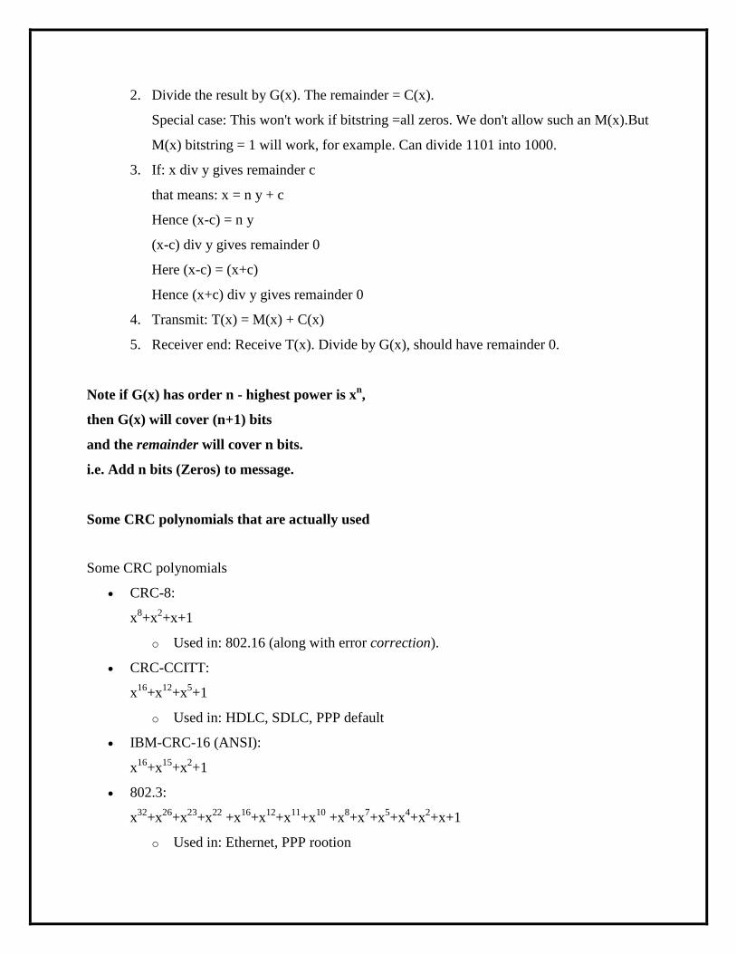
Some CRC polynomials that are actually used
Some CRC polynomials
CRC-8:
x8+x
2+x+1
o Used in: 802.16 (along with error correction).
CRC-CCITT:
x16
+x12
+x5+1
o Used in: HDLC, SDLC, PPP default
IBM-CRC-16 (ANSI):
x16
+x15
+x2+1
802.3:
x32
+x26
+x23
+x22
+x16
+x12
+x11
+x10
+x8+x
7+x
5+x
4+x
2+x+1
o Used in: Ethernet, PPP rootion
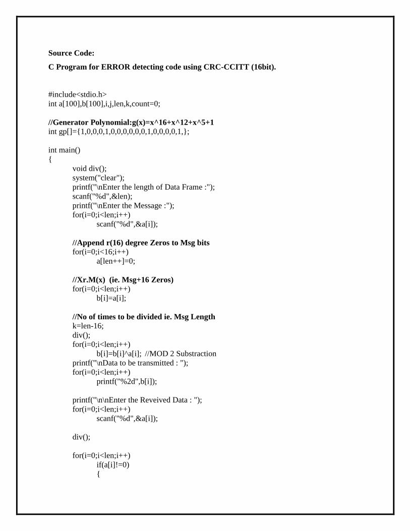
Source Code:
C Program for ERROR detecting code using CRC-CCITT (16bit).
#include<stdio.h>
int a[100],b[100],i,j,len,k,count=0;
//Generator Polynomial:g(x)=x^16+x^12+x^5+1
int gp[]={1,0,0,0,1,0,0,0,0,0,0,1,0,0,0,0,1,};
int main()
{
void div();
system("clear");
printf("\nEnter the length of Data Frame :");
scanf("%d",&len);
printf("\nEnter the Message :");
for(i=0;i<len;i++)
scanf("%d",&a[i]);
//Append r(16) degree Zeros to Msg bits
for(i=0;i<16;i++)
a[len++]=0;
//Xr.M(x) (ie. Msg+16 Zeros)
for(i=0;i<len;i++)
b[i]=a[i];
//No of times to be divided ie. Msg Length
k=len-16;
div();
for(i=0;i<len;i++)
b[i]=b[i]^a[i]; //MOD 2 Substraction
printf("\nData to be transmitted : ");
for(i=0;i<len;i++)
printf("%2d",b[i]);
printf("\n\nEnter the Reveived Data : ");
for(i=0;i<len;i++)
scanf("%d",&a[i]);
div();
for(i=0;i<len;i++)
if(a[i]!=0)
{
printf("\nERROR in Recived Data");
return 0;
}
printf("\nData Recived is ERROR FREE");
}
void div()
{
for(i=0;i<k;i++)
{
if(a[i]==gp[0])
{
for(j=i;j<17+i;j++)
a[j]=a[j]^gp[count++];
}
count=0;
}
}
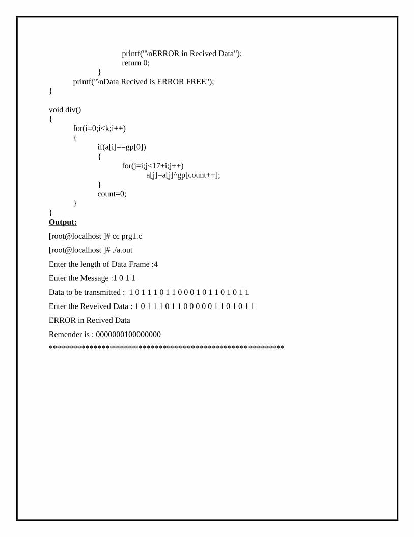
Output:
[root@localhost ]# cc prg1.c
[root@localhost ]# ./a.out
Enter the length of Data Frame :4
Enter the Message :1 0 1 1
Data to be transmitted : 1 0 1 1 1 0 1 1 0 0 0 1 0 1 1 0 1 0 1 1
Enter the Reveived Data : 1 0 1 1 1 0 1 1 0 0 0 0 0 1 1 0 1 0 1 1
ERROR in Recived Data
Remender is : 0000000100000000
**********************************************************

Experiment No: 2 Date:
Distance Vector Algorithm
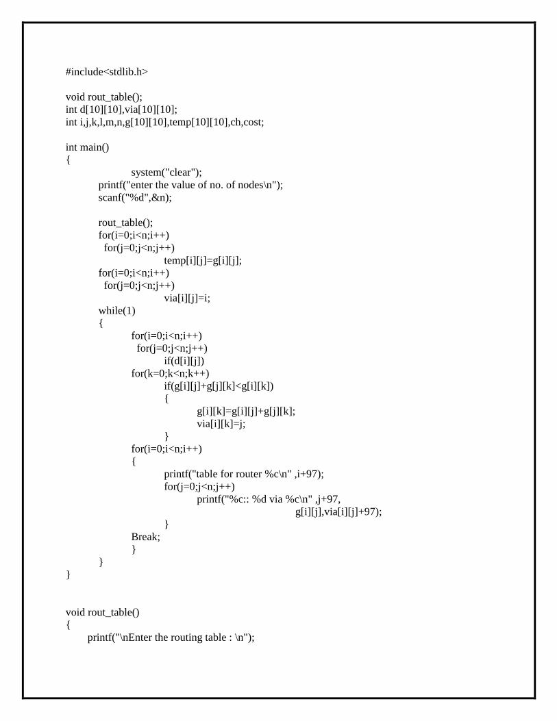
Aim: C Program for Distance Vector Algorithm to find suitable path for transmition
Distance Vector Algorithm is a decentralized routing algorithm that requires that each
router simply inform its neighbors of its routing table. For each network path, the receiving
routers pick the neighbor advertising the lowest cost, then add this entry into its routing table for
re-advertisement. To find the shortest path, Distance Vector Algorithm is based on one of two
basic algorithms: the Bellman-Ford and the Dijkstra algorithms.
Routers that use this algorithm have to maintain the distance tables (which is a one-
dimension array -- "a vector"), which tell the distances and shortest path to sending packets to
each node in the network. The information in the distance table is always upd by exchanging
information with the neighboring nodes. The number of data in the table equals to that of all
nodes in networks (excluded itself). The columns of table represent the directly attached
neighbors whereas the rows represent all destinations in the network. Each data contains the path
for sending packets to each destination in the network and distance/or time to transmit on that
path (we call this as "cost"). The measurements in this algorithm are the number of hops, latency,
the number of outgoing packets, etc.
The starting assumption for distance-vector routing is each node knows the cost of the
link of each of its directly connected neighbors. Next, every node sends a configured message to
its directly connected neighbors containing its own distance table. Now, every node can learn
and up its distance table with cost and next hops for all nodes network. Repeat exchanging until
no more information between the neighbors.
Consider a node A that is interested in routing to destination H via a directly attached
neighbor J. Node A's distance table entry, Dx(Y,Z) is the sum of the cost of the direct-one hop
link between A and J, c(A,J), plus neighboring J's currently known minimum-cost path (shortest
path) from itself(J) to H. That is
Dx(H,J) = c(A,J) + minw{Dj(H,w)} The minw is taken over all the J's
This equation suggests that the form of neighbor-to-neighbor communication that will take place
in the DV algorithm - each node must know the cost of each of its neighbors' minimum-cost path
to each destination. Hence, whenever a node computes a new minimum cost to some destination,
it must inform its neighbors of this new minimum cost.
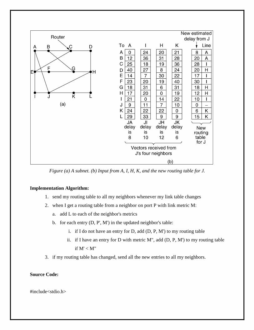
Figure (a) A subnet. (b) Input from A, I, H, K, and the new routing table for J.
Implementation Algorithm:
1. send my routing table to all my neighbors whenever my link table changes
2. when I get a routing table from a neighbor on port P with link metric M:
a. add L to each of the neighbor's metrics
b. for each entry (D, P', M') in the updated neighbor's table:
i. if I do not have an entry for D, add (D, P, M') to my routing table
ii. if I have an entry for D with metric M", add (D, P, M') to my routing table
if M' < M"
3. if my routing table has changed, send all the new entries to all my neighbors.
Source Code:
#include<stdio.h>
#include<stdlib.h>
void rout_table();
int d[10][10],via[10][10];
int i,j,k,l,m,n,g[10][10],temp[10][10],ch,cost;
int main()
{
system("clear");
printf("enter the value of no. of nodes\n");
scanf("%d",&n);
rout_table();
for(i=0;i<n;i++)
for(j=0;j<n;j++)
temp[i][j]=g[i][j];
for(i=0;i<n;i++)
for(j=0;j<n;j++)
via[i][j]=i;
while(1)
{
for(i=0;i<n;i++)
for(j=0;j<n;j++)
if(d[i][j])
for(k=0;k<n;k++)
if(g[i][j]+g[j][k]<g[i][k])
{
g[i][k]=g[i][j]+g[j][k];
via[i][k]=j;
}
for(i=0;i<n;i++)
{
printf("table for router %c\n" ,i+97);
for(j=0;j<n;j++)
printf("%c:: %d via %c\n" ,j+97,
g[i][j],via[i][j]+97);
}
Break;
}
}
}
void rout_table()
{
printf("\nEnter the routing table : \n");
printf("\t|");
for(i=1;i<=n;i++)
printf("%c\t",i+96);
printf("\n");
for(i=0;i<=n;i++)
printf("-------");
printf("\n");
for(i=0;i<n;i++)
{
printf("%c |",i+97);
for(j=0;j<n;j++)
{
scanf("%d",&g[i][j]);
if(g[i][j]!=999)
d[i][j]=1;
}
}
}
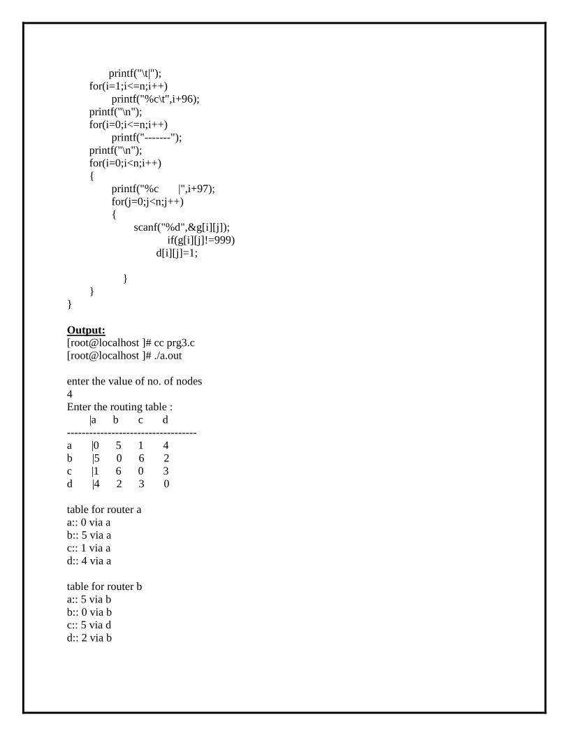
Output: [root@localhost ]# cc prg3.c
[root@localhost ]# ./a.out
enter the value of no. of nodes
4
Enter the routing table :
|a b c d
-----------------------------------
a |0 5 1 4
b |5 0 6 2
c |1 6 0 3
d |4 2 3 0
table for router a
a:: 0 via a
b:: 5 via a
c:: 1 via a
d:: 4 via a
table for router b
a:: 5 via b
b:: 0 via b
c:: 5 via d
d:: 2 via b

table for router c
a:: 1 via c
b:: 5 via d
c:: 0 via c
d:: 3 via c
table for router d
a:: 4 via d
b:: 2 via d
c:: 3 via d
d:: 0 via d
do you want to change the cost(1/0)
1
enter the vertices which you want to change the cost
1 3
enter the cost
2
table for router a
a:: 0 via a
b:: 5 via a
c:: 2 via a
d:: 4 via a
table for router b
a:: 5 via b
b:: 0 via b
c:: 5 via d
d:: 2 via b
table for router c
a:: 2 via c
b:: 5 via d
c:: 0 via c
d:: 3 via c
table for router d
a:: 4 via d
b:: 2 via b
c:: 3 via d
d:: 0 via d
do you want to change the cost(1/0)
0

Experiment No: 3 Date:
Client-server socket programming
Aim: Using TCP/IP Sockets, write a client-server program to make client sending the file name
and the server to send back the contents of the requested file if present.
Sockets are a protocol independent method of creating a connection between processes. Sockets
can be either
Connection based or connectionless: Is a connection established before communication
or does each packet describe the destination?
Packet based or streams based: Are there message boundaries or is it one stream?
Reliable or unreliable: Can messages be lost, duplicated, reordered, or corrupted?
Socket characteristics
Sockets are characterized by their domain, type and transport protocol. Common domains are:
AF_UNIX: address format is UNIX pathname
AF_INET: address format is host and port number
Common types are:
virtual circuit: received in order transmitted and reliably
datagram: arbitrary order, unreliable
Each socket type has one or more protocols. Ex:
TCP/IP (virtual circuits)
UDP (datagram)
Use of sockets:
Connection–based sockets communicate client-server: the server waits for a connection
from the client
Connectionless sockets are peer-to-peer: each process is symmetric.
Socket APIs

socket: creates a socket of a given domain, type, protocol (buy a phone)
bind: assigns a name to the socket (get a telephone number)
listen: specifies the number of pending connections that can be queued for a server
socket. (call waiting allowance)
accept: server accepts a connection request from a client (answer phone)
connect: client requests a connection request to a server (call)
send, sendto: write to connection (speak)
recv, recvfrom: read from connection (listen)
shutdown: end the call
Connection-based communication
Server performs the following actions
socket: create the socket
bind: give the address of the socket on the server
listen: specifies the maximum number of connection requests that can be pending for this
process
accept: establish the connection with a specific client
send, recv: stream-based equivalents of read and write (repeated)
shutdown: end reading or writing
close: release kernel data structures
Client performs the following actions
socket: create the socket
connect: connect to a server
send, recv: (repeated)
shutdown
close
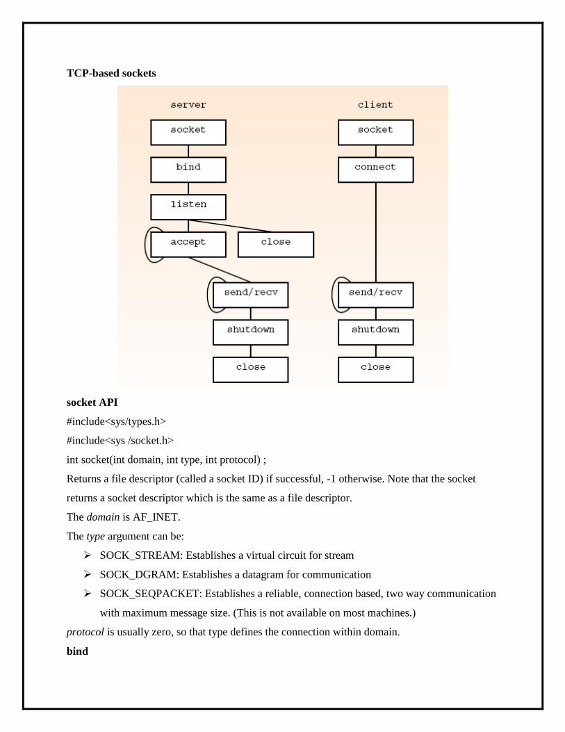
TCP-based sockets
socket API
#include<sys/types.h>
#include<sys /socket.h>
int socket(int domain, int type, int protocol) ;
Returns a file descriptor (called a socket ID) if successful, -1 otherwise. Note that the socket
returns a socket descriptor which is the same as a file descriptor.
The domain is AF_INET.
The type argument can be:
SOCK_STREAM: Establishes a virtual circuit for stream
SOCK_DGRAM: Establishes a datagram for communication
SOCK_SEQPACKET: Establishes a reliable, connection based, two way communication
with maximum message size. (This is not available on most machines.)
protocol is usually zero, so that type defines the connection within domain.
bind
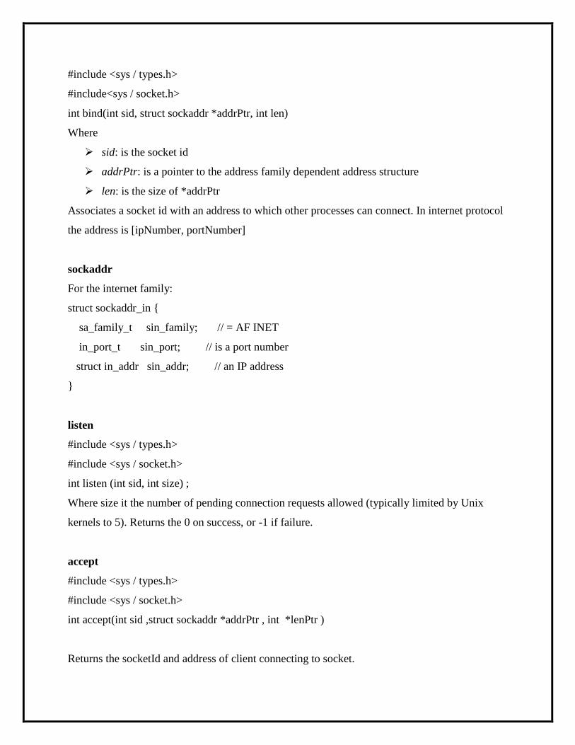
#include <sys / types.h>
#include<sys / socket.h>
int bind(int sid, struct sockaddr *addrPtr, int len)
Where
sid: is the socket id
addrPtr: is a pointer to the address family dependent address structure
len: is the size of *addrPtr
Associates a socket id with an address to which other processes can connect. In internet protocol
the address is [ipNumber, portNumber]
sockaddr
For the internet family:
struct sockaddr_in {
sa_family_t sin_family; // = AF INET
in_port_t sin_port; // is a port number
struct in_addr sin_addr; // an IP address
}
listen
#include <sys / types.h>
#include <sys / socket.h>
int listen (int sid, int size) ;
Where size it the number of pending connection requests allowed (typically limited by Unix
kernels to 5). Returns the 0 on success, or -1 if failure.
accept
#include <sys / types.h>
#include <sys / socket.h>
int accept(int sid ,struct sockaddr *addrPtr , int *lenPtr )
Returns the socketId and address of client connecting to socket.
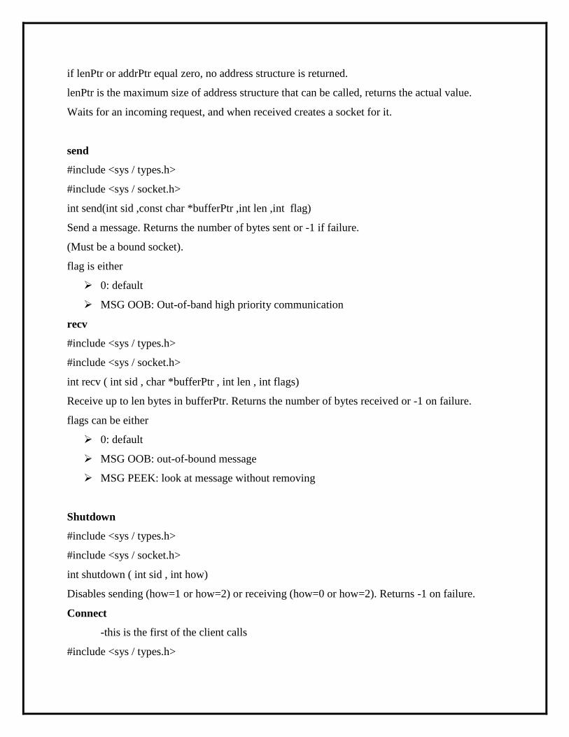
if lenPtr or addrPtr equal zero, no address structure is returned.
lenPtr is the maximum size of address structure that can be called, returns the actual value.
Waits for an incoming request, and when received creates a socket for it.
send
#include <sys / types.h>
#include <sys / socket.h>
int send(int sid ,const char *bufferPtr ,int len ,int flag)
Send a message. Returns the number of bytes sent or -1 if failure.
(Must be a bound socket).
flag is either
0: default
MSG OOB: Out-of-band high priority communication
recv
#include <sys / types.h>
#include <sys / socket.h>
int recv ( int sid , char *bufferPtr , int len , int flags)
Receive up to len bytes in bufferPtr. Returns the number of bytes received or -1 on failure.
flags can be either
0: default
MSG OOB: out-of-bound message
MSG PEEK: look at message without removing
Shutdown
#include <sys / types.h>
#include <sys / socket.h>
int shutdown ( int sid , int how)
Disables sending (how=1 or how=2) or receiving (how=0 or how=2). Returns -1 on failure.
Connect
-this is the first of the client calls
#include <sys / types.h>
#include <sys / socket.h>
int connect ( int sid , struct sockaddr *addrPtr , int len)
Specifies the destination to form a connection with (addrPtr), and returns a 0 if successful, -1
otherwise.
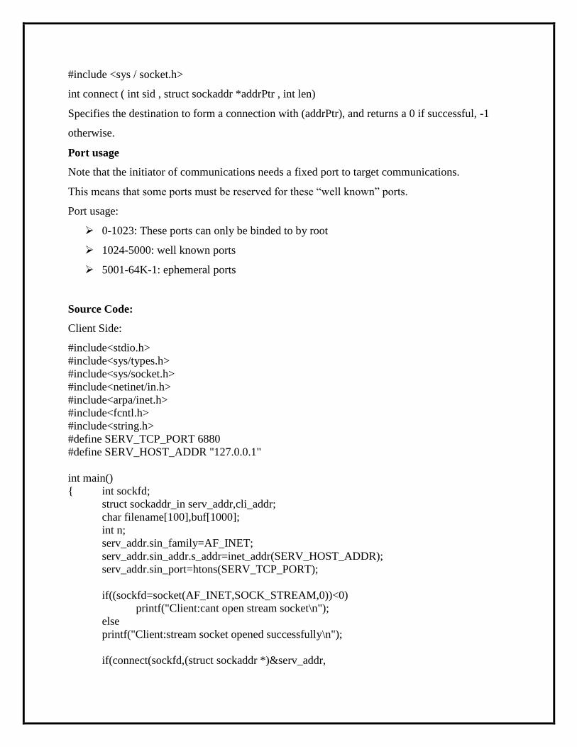
Port usage
Note that the initiator of communications needs a fixed port to target communications.
This means that some ports must be reserved for these ―well known‖ ports.
Port usage:
0-1023: These ports can only be binded to by root
1024-5000: well known ports
5001-64K-1: ephemeral ports
Source Code:
Client Side:
#include<stdio.h>
#include<sys/types.h>
#include<sys/socket.h>
#include<netinet/in.h>
#include<arpa/inet.h>
#include<fcntl.h>
#include<string.h>
#define SERV_TCP_PORT 6880
#define SERV_HOST_ADDR "127.0.0.1"
int main()
{ int sockfd;
struct sockaddr_in serv_addr,cli_addr;
char filename[100],buf[1000];
int n;
serv_addr.sin_family=AF_INET;
serv_addr.sin_addr.s_addr=inet_addr(SERV_HOST_ADDR);
serv_addr.sin_port=htons(SERV_TCP_PORT);
if((sockfd=socket(AF_INET,SOCK_STREAM,0))<0)
printf("Client:cant open stream socket\n");
else
printf("Client:stream socket opened successfully\n");
if(connect(sockfd,(struct sockaddr *)&serv_addr,
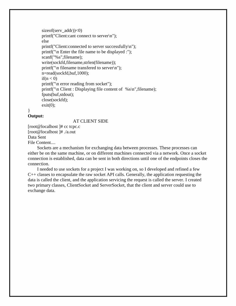
sizeof(serv_addr))<0)
printf("Client:cant connect to server\n");
else
printf("Client:connected to server successfully\n");
printf("\n Enter the file name to be displayed :");
scanf("%s",filename);
write(sockfd,filename,strlen(filename));
printf("\n filename transfered to server\n");
n=read(sockfd,buf,1000);
if(n < 0)
printf("\n error reading from socket");
printf("\n Client : Displaying file content of %s\n",filename);
fputs(buf,stdout);
close(sockfd);
exit(0);
}
Output:
AT CLIENT SIDE
[root@localhost ]# cc tcpc.c
[root@localhost ]# ./a.out
Data Sent
File Content....
Sockets are a mechanism for exchanging data between processes. These processes can
either be on the same machine, or on different machines connected via a network. Once a socket
connection is established, data can be sent in both directions until one of the endpoints closes the
connection.
I needed to use sockets for a project I was working on, so I developed and refined a few
C++ classes to encapsulate the raw socket API calls. Generally, the application requesting the
data is called the client, and the application servicing the request is called the server. I created
two primary classes, ClientSocket and ServerSocket, that the client and server could use to
exchange data.
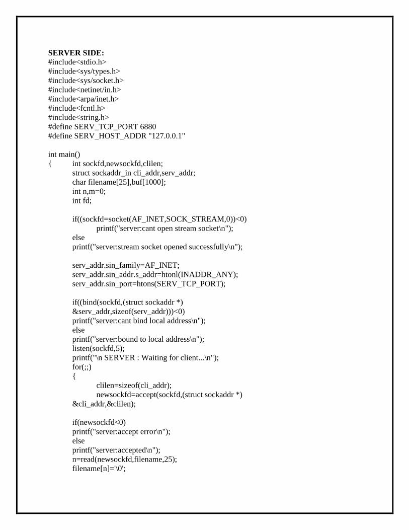
SERVER SIDE:
#include<stdio.h>
#include<sys/types.h>
#include<sys/socket.h>
#include<netinet/in.h>
#include<arpa/inet.h>
#include<fcntl.h>
#include<string.h>
#define SERV_TCP_PORT 6880
#define SERV_HOST_ADDR "127.0.0.1"
int main()
{ int sockfd,newsockfd,clilen;
struct sockaddr_in cli_addr,serv_addr;
char filename[25],buf[1000];
int n,m=0;
int fd;
if((sockfd=socket(AF_INET,SOCK_STREAM,0))<0)
printf("server:cant open stream socket\n");
else
printf("server:stream socket opened successfully\n");
serv_addr.sin_family=AF_INET;
serv_addr.sin_addr.s_addr=htonl(INADDR_ANY);
serv_addr.sin_port=htons(SERV_TCP_PORT);
if((bind(sockfd,(struct sockaddr *)
&serv_addr,sizeof(serv_addr)))<0)
printf("server:cant bind local address\n");
else
printf("server:bound to local address\n");
listen(sockfd,5);
printf("\n SERVER : Waiting for client...\n");
for(;;)
{
clilen=sizeof(cli_addr);
newsockfd=accept(sockfd,(struct sockaddr *)
&cli_addr,&clilen);
if(newsockfd<0)
printf("server:accept error\n");
else
printf("server:accepted\n");
n=read(newsockfd,filename,25);
filename[n]='\0';
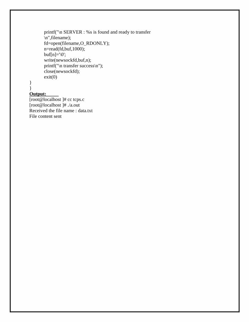
printf("\n SERVER : %s is found and ready to transfer
\n",filename);
fd=open(filename,O_RDONLY);
n=read(fd,buf,1000);
buf[n]='\0';
write(newsockfd,buf,n);
printf("\n transfer success\n");
close(newsockfd);
exit(0)
}
}
Output: [root@localhost ]# cc tcps.c
[root@localhost ]# ./a.out
Received the file name : data.txt
File content sent

Experiment No: 4 Date:
Client-Server Communication Using Message Queues or FIFO
Aim: C Program for CLIENT SERVER communication using message Queues or FIFOs as IPC
channels that client sends the file name and the server to send back the contents of the requested
file if present.
Message Queues
Message queues are one of the three different types of System V IPC mechanisms. This
mechanism enables processes to send information to each other asynchronously. The word
asynchronous in the present context signifies that the sender process continues with its execution
without waiting for the receiver to receive or acknowledge the information. On the other side, the
receiver does not wait if no messages are there in the queue. The queue being referred to here is
the queue implemented and maintained by the kernel.
Let us now take a look at the system calls associated with this mechanism.
a. msgget: This, in a way similar to shmget, gets a message queue identifier. The format is
int msgget(ket_t key, int msgflg);
The first argument is a unique key, which can be generated by using ftok algorithm. The
second argument is the flag which can be IPC_CREAT, IPC_PRIVATE, or one of the
other valid possibilities (see the man page); the permissions (read and/or write) are logically
ORed with the flags. msgget returns an identifier associated with the key. This identifier can
be used for further processing of the message queue associated with the identifier.
b. msgctl: This controls the operations on the message queue. The format is
int msgctl(int msqid, int cmd, struct msqid_ds *buf);
Here msqid is the message queue identifier returned by msgget. The second argument is
cmd, which indicates which action is to be taken on the message queue. The third argument
is a buffer of type struct msqid_ds. Each message queue has this structure associated with it;
it is composed of records for queues to be identified by the kernel. This structure also defines
the current status of the message queue. If one of the cmds is IPC_SET, some fields in the
msqid_ds structure (pointed by the third argument) will be set to the specified values. See
the man page for the details.
c. msgsnd: This is for sending messages. The format is
int msgsnd(int msqid, struct msgbuf *msgp, size_t msgsz, int msgflg);

The first argument is the message queue identifier returned by msgget. The second
argument is a structure that the calling process allocates. A call to msgsnd appends a copy of
the message pointed to by msgp to the message queue identified by msqid. The third
argument is the size of the message text within the msgbuf structure. The fourth argument is
the flag that specify one of several actions to be taken as and when a specific situation arises.
d. msgrcv: This is for receiving messages. The format is
ssize_t msgrcv(int msqid, struct msgbuf *msgp, size_t msgsz, long msgtyp, int msgflg);
Besides the four arguments mentioned above for msgsnd, we also have msgtyp, which
specifies the type of message requested.
FIFO :
FIFOs (first in, first out) are similar to the working of pipes. One major feature of pipe is
that the data flowing through the communication medium is transient, that is, data once read
from the read descriptor cannot be read again. Also, if we write data continuously into the write
descriptor, then we will be able to read the data only in the order in which the data was written.
One can experiment with that by doing successive writes or reads to the respective descriptors.
FIFOs also provide half-duplex flow of data just like pipes. The difference between fifos
and pipes is that the former is identified in the file system with a name, while the latter is not.
That is, fifos are named pipes. Fifos are identified by an access point which is a file within the
file system, whereas pipes are identified by an access point which is simply an allotted inode.
Another major difference between fifos and pipes is that fifos last throughout the life-cycle of the
system, while pipes last only during the life-cycle of the process in which they were created. To
make it more clear, fifos exist beyond the life of the process. Since they are identified by the file
system, they remain in the hierarchy until explicitly removed using unlink, but pipes are
inherited only by related processes, that is, processes which are descendants of a single process.
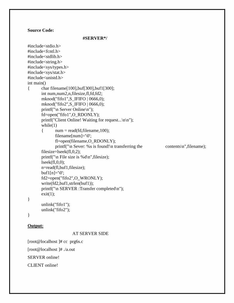
Source Code:
#SERVER*/
#include<stdio.h>
#include<fcntl.h>
#include<stdlib.h>
#include<string.h>
#include<sys/types.h>
#include<sys/stat.h>
#include<unistd.h>
int main()
{ char filename[100],buf[300],buf1[300];
int num,num2,n,filesize,fl,fd,fd2;
mknod("fifo1",S_IFIFO | 0666,0);
mknod("fifo2",S_IFIFO | 0666,0);
printf("\n Server Online\n");
fd=open("fifo1",O_RDONLY);
printf("Client Online! Waiting for request...\n\n");
while(1)
{ num = read(fd,filename,100);
filename[num]='\0';
fl=open(filename,O_RDONLY);
printf("\n Sever: %s is found!\n transferring the contents\n",filename);
filesize=lseek(fl,0,2);
printf("\n File size is %d\n",filesize);
lseek(fl,0,0);
n=read(fl,buf1,filesize);
buf1[n]='\0';
fd2=open("fifo2",O_WRONLY);
write(fd2,buf1,strlen(buf1));
printf("\n SERVER :Transfer completed\n");
exit(1);
}
unlink("fifo1");
unlink("fifo2");
}
Output:
AT SERVER SIDE
[root@localhost ]# cc prg6s.c
[root@localhost ]# ./a.out
SERVER online!
CLIENT online!
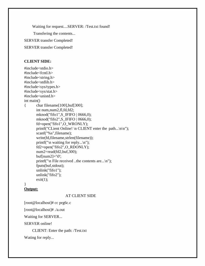
Waiting for request....SERVER: /Test.txt found!
Transfering the contents...
SERVER transfer Completed!
SERVER transfer Completed!
CLIENT SIDE:
#include<stdio.h>
#include<fcntl.h>
#include<string.h>
#include<stdlib.h>
#include<sys/types.h>
#include<sys/stat.h>
#include<unistd.h>
int main()
{ char filename[100],buf[300];
int num,num2,fl,fd,fd2;
mknod("fifo1",S_IFIFO | 0666,0);
mknod("fifo2",S_IFIFO | 0666,0);
fd=open("fifo1",O_WRONLY);
printf("CLient Online! \n CLIENT enter the path...\n\n");
scanf("%s",filename);
write(fd,filename,strlen(filename));
printf("\n waiting for reply...\n");
fd2=open("fifo2",O_RDONLY);
num2=read(fd2,buf,300);
buf[num2]='\0';
printf("\n File received ..the contents are...\n");
fputs(buf,stdout);
unlink("fifo1");
unlink("fifo2");
exit(1);
}
Output:
AT CLIENT SIDE
[root@localhost]# cc prg6c.c
[root@localhost]# ./a.out
Waiting for SERVER...
SERVER online!
CLIENT: Enter the path: /Test.txt
Wating for reply...
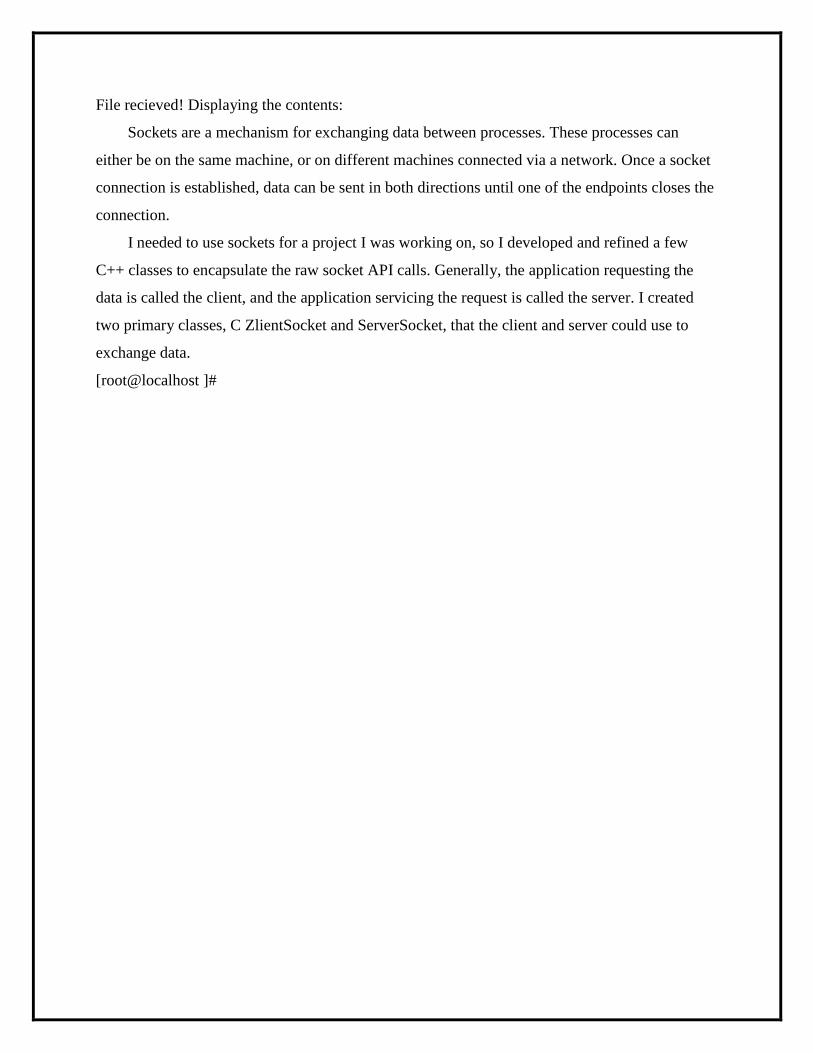
File recieved! Displaying the contents:
Sockets are a mechanism for exchanging data between processes. These processes can
either be on the same machine, or on different machines connected via a network. Once a socket
connection is established, data can be sent in both directions until one of the endpoints closes the
connection.
I needed to use sockets for a project I was working on, so I developed and refined a few
C++ classes to encapsulate the raw socket API calls. Generally, the application requesting the
data is called the client, and the application servicing the request is called the server. I created
two primary classes, C ZlientSocket and ServerSocket, that the client and server could use to
exchange data.
[root@localhost ]#

Experiment No: 5 Date:
RSA Algorithm to Encrypt and Decrypt the Data
Aim: C Program for Simple RSA Algorithm to encrypt and decrypt the data
The RSA algorithm can be used for both public key encryption and digital signatures. Its
security is based on the difficulty of factoring large integers.
The RSA algorithm's efficiency requires a fast method for performing the modular
exponentiation operation. A less efficient, conventional method includes raising a number (the
input) to a power (the secret or public key of the algorithm, denoted e and d, respectively) and
taking the remainder of the division with N. A straight-forward implementation performs these
two steps of the operation sequentially: first, raise it to the power and second, apply modulo.
A very simple example of RSA encryption
This is an extremely simple example using numbers you can work out on a pocket
calculator (those of you over the age of 35 can probably even do it by hand on paper).
1. Select primes p = 11, q = 3.
2. n = pq = 11.3 = 33
phi = (p-1)(q-1) = 10.2 = 20
3. Choose e=3
Check gcd(e, p-1) = gcd(3, 10) = 1 (i.e. 3 and 10 have no common factors except 1),
and check gcd(e, q-1) = gcd(3, 2) = 1
therefore gcd(e, phi) = gcd(e, (p-1)(q-1)) = gcd(3, 20) = 1
4. Compute d such that ed ≡ 1 (mod phi)
i.e. compute d = e^-1
mod phi = 3^-1
mod 20
i.e. find a value for d such that phi divides (ed-1)
i.e. find d such that 20 divides 3d-1.
Simple testing (d = 1, 2, ...) gives d = 7
Check: ed-1 = 3.7 - 1 = 20, which is divisible by phi.
5. Public key = (n, e) = (33, 3)
Private key = (n, d) = (33, 7).
This is actually the smallest possible value for the modulus n for which the RSA
algorithm works.

Now say we want to encrypt the message m = 7,
c = m^e
mod n = 7^3
mod 33 = 343 mod 33 = 13.
Hence the ciphertext c = 13.
To check decryption we compute
m' = c^d
mod n = 13^7
mod 33 = 7.
Note that we don't have to calculate the full value of 13 to the power 7 here. We can
make use of the fact that a = bc mod n = (b mod n).(c mod n) mod n so we can break down a
potentially large number into its components and combine the results of easier, smaller
calculations to calculate the final value.
One way of calculating m' is as follows:-
m' = 13^7
mod 33 = 13^(3+3+1)
mod 33 = 13^3
.13^3
.13 mod 33
= (13^3
mod 33).(13^3
mod 33).(13 mod 33) mod 33
= (2197 mod 33).(2197 mod 33).(13 mod 33) mod 33
= 19.19.13 mod 33 = 4693 mod 33
= 7.
Now if we calculate the cipher text c for all the possible values of m (0 to 32), we get
m 0 1 2 3 4 5 6 7 8 9 10 11 12 13 14 15 16
c 0 1 8 27 31 26 18 13 17 3 10 11 12 19 5 9 4
m 17 18 19 20 21 22 23 24 25 26 27 28 29 30 31 32
c 29 24 28 14 21 22 23 30 16 20 15 7 2 6 25 32
Note that all 33 values of m (0 to 32) map to a unique code c in the same range in a sort
of random manner. In this case we have nine values of m that map to the same value of c - these
are known as unconcealed messages. m = 0 and 1 will always do this for any N, no matter how
large. But in practice, higher values shouldn't be a problem when we use large values for N.
If we wanted to use this system to keep secrets, we could let A=2, B=3, ..., Z=27. (We
specifically avoid 0 and 1 here for the reason given above). Thus the plaintext message
"HELLOWORLD" would be represented by the set of integers m1, m2, ...
{9,6,13,13,16,24,16,19,13,5}
Using our table above, we obtain ciphertext integers c1, c2, ...
{3,18,19,19,4,30,4,28,19,26}

Note that this example is no more secure than using a simple Caesar substitution cipher,
but it serves to illustrate a simple example of the mechanics of RSA encryption.
Remember that calculating m^e mod n is easy, but calculating the inverse c^-e mod n is
very difficult, well, for large n's anyway. However, if we can factor n into its prime factors p and
q, the solution becomes easy again, even for large n's. Obviously, if we can get hold of the secret
exponent d, the solution is easy, too.
Key Generation Algorithm
1. Generate two large random primes, p and q, of approximately equal size such that
their product n = pq is of the required bit length, e.g. 1024 bits. [See note 1].
2. Compute n = pq and (φ) phi = (p-1)(q-1).
3. Choose an integer e, 1 < e < phi, such that gcd(e, phi) = 1. [See note 2].
4. Compute the secret exponent d, 1 < d < phi, such that
ed ≡ 1 (mod phi). [See note 3].
5. The public key is (n, e) and the private key is (n, d). The values of p, q, and phi
should also be kept secret.
n is known as the modulus.
e is known as the public exponent or encryption exponent.
d is known as the secret exponent or decryption exponent.
Encryption
Sender A does the following:-
1. Obtains the recipient B's public key (n, e).
2. Represents the plaintext message as a positive integer m [see note 4].
3. Computes the ciphertext c = m^e
mod n.
4. Sends the ciphertext c to B.
Decryption
Recipient B does the following:-
1. Uses his private key (n, d) to compute m = c^d
mod n.
2. Extracts the plaintext from the integer representative m.
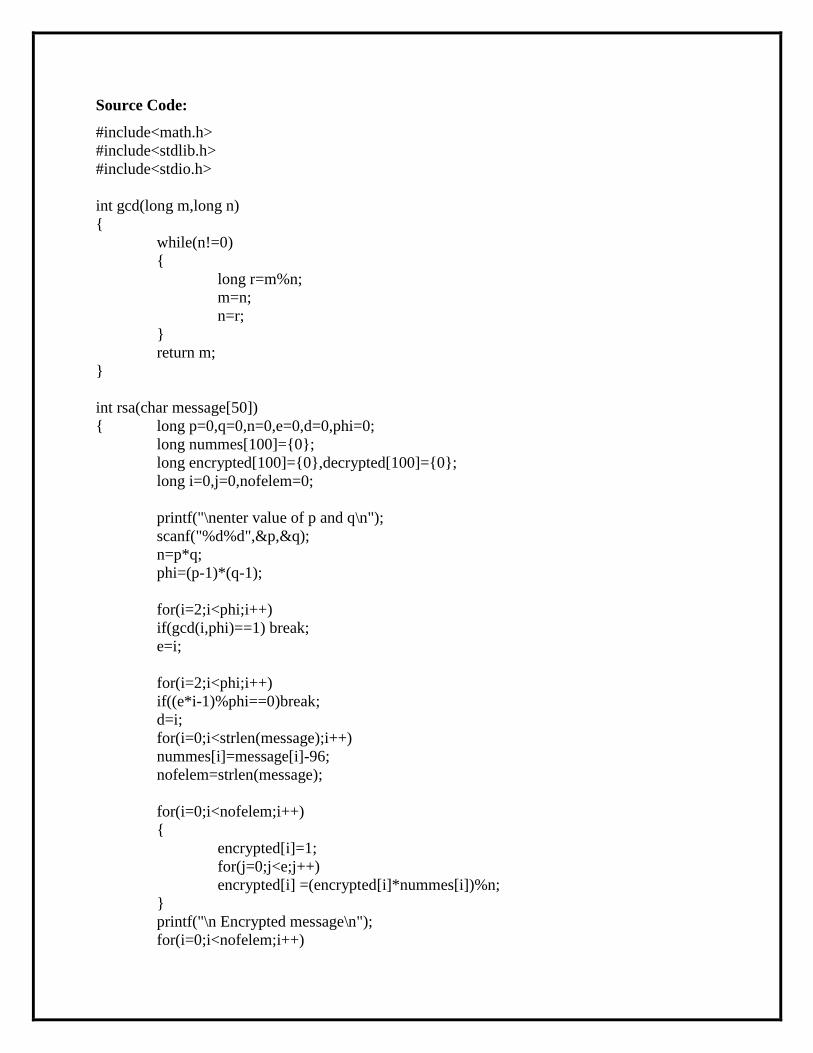
Source Code:
#include<math.h>
#include<stdlib.h>
#include<stdio.h>
int gcd(long m,long n)
{
while(n!=0)
{
long r=m%n;
m=n;
n=r;
}
return m;
}
int rsa(char message[50])
{ long p=0,q=0,n=0,e=0,d=0,phi=0;
long nummes[100]={0};
long encrypted[100]={0},decrypted[100]={0};
long i=0,j=0,nofelem=0;
printf("\nenter value of p and q\n");
scanf("%d%d",&p,&q);
n=p*q;
phi=(p-1)*(q-1);
for(i=2;i<phi;i++)
if(gcd(i,phi)==1) break;
e=i;
for(i=2;i<phi;i++)
if((e*i-1)%phi==0)break;
d=i;
for(i=0;i<strlen(message);i++)
nummes[i]=message[i]-96;
nofelem=strlen(message);
for(i=0;i<nofelem;i++)
{
encrypted[i]=1;
for(j=0;j<e;j++)
encrypted[i] =(encrypted[i]*nummes[i])%n;
}
printf("\n Encrypted message\n");
for(i=0;i<nofelem;i++)
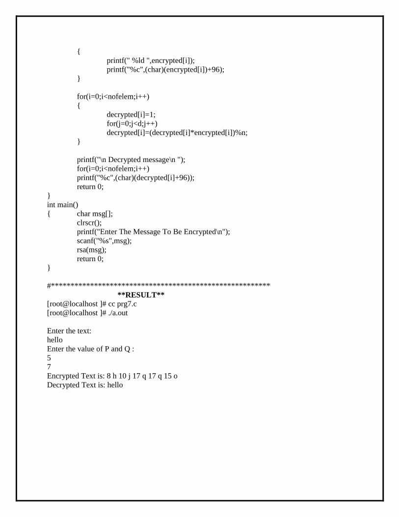
{
printf(" %ld ",encrypted[i]);
printf("%c",(char)(encrypted[i])+96);
}
for(i=0;i<nofelem;i++)
{
decrypted[i]=1;
for(j=0;j<d;j++)
decrypted[i]=(decrypted[i]*encrypted[i])%n;
}
printf("\n Decrypted message\n ");
for(i=0;i<nofelem;i++)
printf("%c",(char)(decrypted[i]+96));
return 0;
}
int main()
{ char msg[];
clrscr();
printf("Enter The Message To Be Encrypted\n");
scanf("%s",msg);
rsa(msg);
return 0;
}
#********************************************************
**RESULT**
[root@localhost ]# cc prg7.c
[root@localhost ]# ./a.out
Enter the text:
hello
Enter the value of P and Q :
5
7
Encrypted Text is: 8 h 10 j 17 q 17 q 15 o
Decrypted Text is: hello
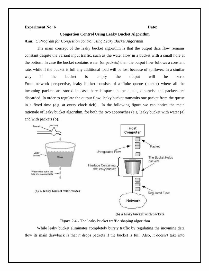
Experiment No: 6 Date:
Congestion Control Using Leaky Bucket Algorithm
Aim: C Program for Congestion control using Leaky Bucket Algorithm
The main concept of the leaky bucket algorithm is that the output data flow remains
constant despite the variant input traffic, such as the water flow in a bucket with a small hole at
the bottom. In case the bucket contains water (or packets) then the output flow follows a constant
rate, while if the bucket is full any additional load will be lost because of spillover. In a similar
way if the bucket is empty the output will be zero.
From network perspective, leaky bucket consists of a finite queue (bucket) where all the
incoming packets are stored in case there is space in the queue, otherwise the packets are
discarded. In order to regulate the output flow, leaky bucket transmits one packet from the queue
in a fixed time (e.g. at every clock tick). In the following figure we can notice the main
rationale of leaky bucket algorithm, for both the two approaches (e.g. leaky bucket with water (a)
and with packets (b)).
Figure 2.4 - The leaky bucket traffic shaping algorithm
While leaky bucket eliminates completely bursty traffic by regulating the incoming data
flow its main drawback is that it drops packets if the bucket is full. Also, it doesn’t take into
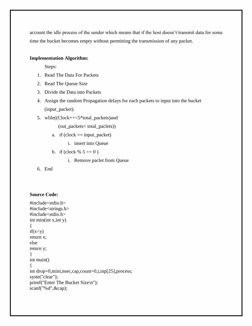
account the idle process of the sender which means that if the host doesn’t transmit data for some
time the bucket becomes empty without permitting the transmission of any packet.
Implementation Algorithm:
Steps:
1. Read The Data For Packets
2. Read The Queue Size
3. Divide the Data into Packets
4. Assign the random Propagation delays for each packets to input into the bucket
(input_packet).
5. wlile((Clock++<5*total_packets)and
(out_packets< total_paclets))
a. if (clock == input_packet)
i. insert into Queue
b. if (clock % 5 == 0 )
i. Remove paclet from Queue
6. End
Source Code:
#include<stdio.h>
#include<strings.h>
#include<stdio.h>
int min(int x,int y)
{
if(x<y)
return x;
else
return y;
}
int main()
{
int drop=0,mini,nsec,cap,count=0,i,inp[25],process;
syste("clear");
printf("Enter The Bucket Size\n");
scanf("%d",&cap);
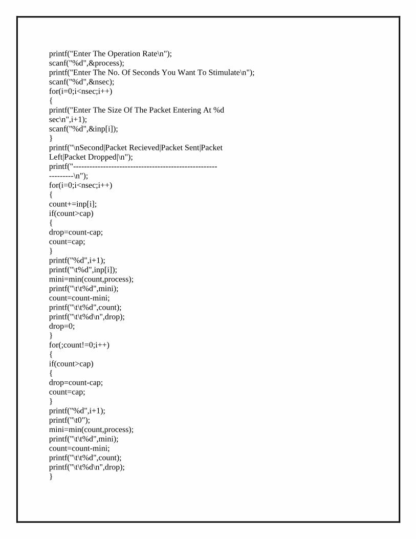
printf("Enter The Operation Rate\n");
scanf("%d",&process);
printf("Enter The No. Of Seconds You Want To Stimulate\n");
scanf("%d",&nsec);
for(i=0;i<nsec;i++)
{
printf("Enter The Size Of The Packet Entering At %d
sec\n",i+1);
scanf("%d",&inp[i]);
}
printf("\nSecond|Packet Recieved|Packet Sent|Packet
Left|Packet Dropped|\n");
printf("-----------------------------------------------------
---------\n");
for(i=0;i<nsec;i++)
{
count+=inp[i];
if(count>cap)
{
drop=count-cap;
count=cap;
}
printf("%d",i+1);
printf("\t%d",inp[i]);
mini=min(count,process);
printf("\t\t%d",mini);
count=count-mini;
printf("\t\t%d",count);
printf("\t\t%d\n",drop);
drop=0;
}
for(;count!=0;i++)
{
if(count>cap)
{
drop=count-cap;
count=cap;
}
printf("%d",i+1);
printf("\t0");
mini=min(count,process);
printf("\t\t%d",mini);
count=count-mini;
printf("\t\t%d",count);
printf("\t\t%d\n",drop);
}
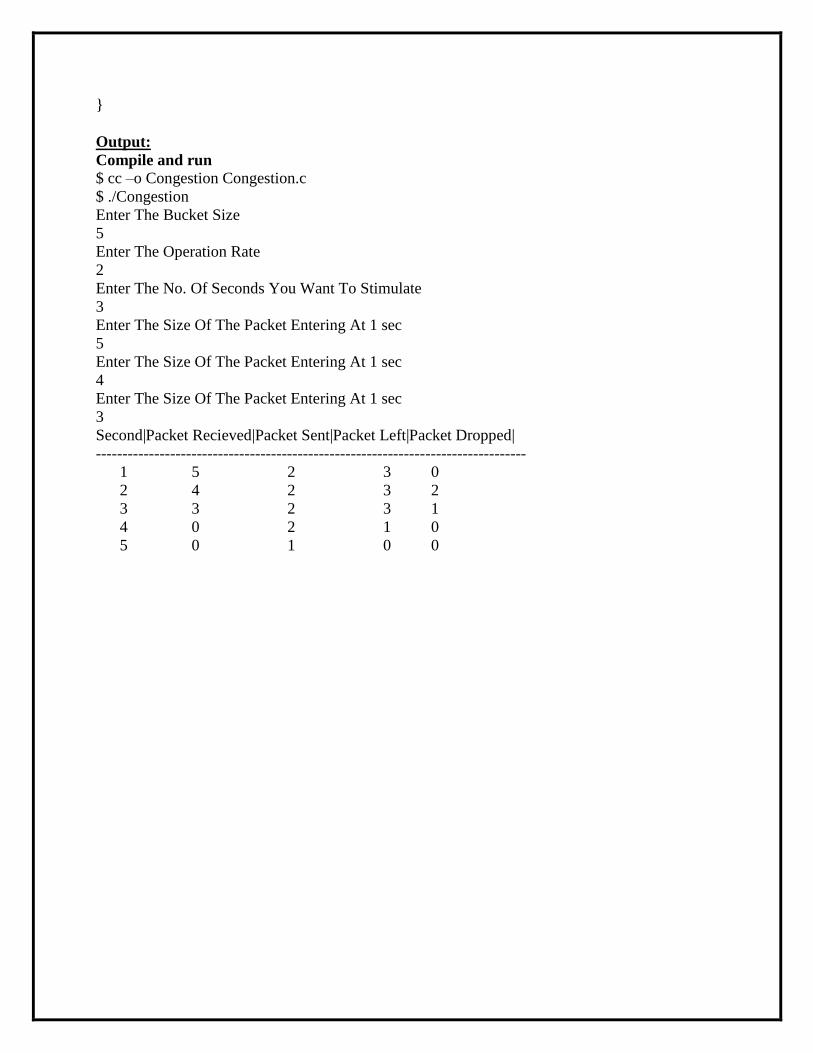
}
Output:
Compile and run
$ cc –o Congestion Congestion.c
$ ./Congestion
Enter The Bucket Size
5
Enter The Operation Rate
2
Enter The No. Of Seconds You Want To Stimulate
3
Enter The Size Of The Packet Entering At 1 sec
5
Enter The Size Of The Packet Entering At 1 sec
4
Enter The Size Of The Packet Entering At 1 sec
3
Second|Packet Recieved|Packet Sent|Packet Left|Packet Dropped|
---------------------------------------------------------------------------------
1 5 2 3 0
2 4 2 3 2
3 3 2 3 1
4 0 2 1 0
5 0 1 0 0

VIVA QUESTIONS
1. What are functions of different layers?
2. Differentiate between TCP/IP Layers and OSI Layers
3. Why header is required?
4. What is the use of adding header and trailer to frames?
5. What is encapsulation?
6. Why fragmentation requires?
7. What is MTU?
8. Which layer imposes MTU?
9. Differentiate between flow control and congestion control.
10. Differentiate between Point-to-Point Connection and End-to-End connections.
11. What are protocols running in different layers?
12. What is Protocol Stack?
13. Differentiate between TCP and UDP.
14. Differentiate between Connectionless and connection oriented connection.
15. Why frame sorting is required?
16. What is meant by subnet?
17. What is meant by Gateway?
18. What is an IP address?
19. What is MAC address?
20. Why IP address is required when we have MAC address?
21. What is meant by port?
22. What are ephemerical port number and well known port numbers?
23. What is a socket?
24. What are the parameters of socket()?
25. Describe bind(), listen(), accept(),connect(), send() and recv().
26. What are system calls? Mention few of them.
27. What is IPC? Name three techniques.
28. Explain mkfifo(), open(), close() with parameters.
29. What is meant by file descriptor?
30. What is meant by traffic shaping?

31. How do you classify congestion control algorithms?
32. Differentiate between Leaky bucket and Token bucket.
33. How do you implement Leaky bucket?
34. How do you generate busty traffic?
35. What is the polynomial used in CRC-CCITT?
36. What are the other error detection algorithms?
37. What is difference between CRC and Hamming code?
38. Why Hamming code is called 7,4 code?
39. What is odd parity and even parity?
40. What is meant by syndrome?
41. What is generator matrix?
42. What is spanning tree?
43. Differentiate between Prim’s and Kruskal’s algorithm.
44. What are Routing algorithms?
45. How do you classify routing algorithms? Give examples for each.
46. What are drawbacks in distance vector algorithm?
47. How routers update distances to each of its neighbor?
48. How do you overcome count to infinity problem?
49. What is cryptography?
50. How do you classify cryptographic algorithms?
51. What is public key?
52. What is private key?
53. What are key, ciphertext and plaintext?
54. What is simulation?
55. What are advantages of simulation?
56. Differentiate between Simulation and Emulation.
57. What is meant by router?
58. What is meant by bridge?
59. What is meant by switch?
60. What is meant by hub?
61. Differentiate between route, bridge, switch and hub.

62. What is ping and telnet?
63. What is FTP?
64. What is BER?
65. What is meant by congestion window?
66. What is BSS?
67. What is incoming throughput and outgoing throughput?
68. What is collision?
69. How do you generate multiple traffics across different sender-receiver pairs?
70. How do you setup Ethernet LAN?
71. What is meant by mobile host?
72. What is meant by NCTUns?
73. What are dispatcher, coordinator and nctunsclient?
74. Name few other Network simulators
75. Differentiate between logical and physical address.
76. Which address gets affected if a system moves from one place to another place?
77. What is ICMP? What are uses of ICMP? Name few.
78. Which layer implements security for data?
REFERENCE
1. Communication Networks: Fundamental Concepts and Key Architectures - Alberto
Leon, Garcia and Indra Widjaja, 3rd
Edition, Tata McGraw- Hill, 2004.
2. Data and Computer Communication, William Stallings, 8th
tEdition, Pearson Education,
2007.
3. Computer Networks: A Systems Approach - Larry L. Peterson and Bruce S. David, 4th
Edition, Elsevier, 2007.
4. Introduction to Data Communications and Networking – Wayne Tomasi, Pearson
Education, 2005.
5. Communication Networks – Fundamental Concepts and Key architectures – Alberto
Leon- Garcia and Indra Widjaja:, 2rd
Edition, Tata McGraw-Hill, 2004
6. Computer and Communication Networks – Nader F. Mir:, Pearson Education, 2007.