Embed Size (px)
Citation preview

Network Operation Strategiesfor Efficient Localization andNavigationThis paper provides network operation strategies, including node prioritization, node
activation, and node deployment to improve the localization performance and prolong
the network lifetime.
By MOE Z. WIN , Fellow IEEE, WENHAN DAI , Student Member IEEE, YUAN SHEN , Member IEEE,
GEORGE CHRISIKOS, Fellow IEEE, AND H. VINCENT POOR , Fellow IEEE
ABSTRACT | Reliable and accurate position information is of
great importance for many mass-market and emerging appli-
cations. Network localization and navigation (NLN) is a promis-
ing paradigm to provide such information ubiquitously, where
a network of nodes is used to aid in localizing its members. This
paper explores various network operation strategies, which
play an essential role in NLN as they determine the network
lifetime and localization accuracy. Efficient network operation
requires several functionalities, including node prioritization,
node activation, and node deployment. The roles of these func-
tionalities are described and different techniques for imple-
menting respective functionalities via algorithmic modules are
introduced. Some important concepts such as cooperative
operation, robustness guarantee, and distributed design in
the development of the network operation strategies are also
introduced. Finally, numerical results are provided to demon-
Manuscript received September 7, 2017; revised April 8, 2018; accepted April 9,
2018. Date of current version July 25, 2018. This work was supported in part by
the U.S. Office of Naval Research under Grant N00014-16-1-2141; in part by the
U.S. National Science Foundation under Grants CNS-1702808 and
ECCS-1647198, and in part by the MIT Institute for Soldier Nanotechnologies.
(Corresponding author: Moe Z. Win.)
M. Z. Win is with the Laboratory for Information and Decision Systems,
Massachusetts Institute of Technology, Cambridge, MA 02139 USA (e-mail:
W. Dai is with the Wireless Information and Network Sciences Laboratory,
Massachusetts Institute of Technology, Cambridge, MA 02139 USA (e-mail:
Y. Shen was with the Wireless Information and Network Sciences Laboratory,
Massachusetts Institute of Technology, Cambridge, MA 02139 USA, and is now
with the Department of Electronic Engineering, Tsinghua University and Beijing
National Research Center for Information Science and Technology, Beijing
100084, China (e-mail: [email protected]).
G. Chrisikos is with Qualcomm Inc., San Diego, CA 92121 USA (e-mail:
H. V. Poor is with the Department of Electrical Engineering, Princeton
University, Princeton, NJ 08544 USA (e-mail: [email protected]).
Digital Object Identifier 10.1109/JPROC.2018.2835314
strate the localization performance improvement attributed to
the optimized network operation strategies.
KEYWORDS | Deployment; localization; navigation; optimiza-
tion; resource allocation; scheduling; wireless network
I. I N T R O D U C T I O N
Location awareness using wireless signals is critical for
many mobile applications [1]–[6], including autonomous
driving [7]–[9], assisted living [10]–[12], Internet-
of-Things [13]–[16], crowdsensing [17]–[20], medical
services [21]–[23], as well as search-and-rescue operations
[24]–[26]. In outdoor scenarios, global navigation satellite
systems (GNSSs) can provide meter-level localization
accuracy around the earth through a constellation of
satellites [27]–[31]. However, the effectiveness of GNSS
is limited in challenging propagation environments, such
as inside buildings and in urban canyons, due to signal
degradation or blockage by obstacles [32]. To complement
GNSS in these challenging propagation environments,
wireless localization networks have been developed in
the past decades for providing high-accuracy location
awareness [33]–[39].
In a typical wireless localization network, there are
two types of nodes, referred to as anchors and agents
[40]–[42]. Anchors have perfectly known positions,
whereas agents have unknown positions. For example,
anchor nodes may consist of WiFi access points or cel-
lular base stations, and agent nodes may consist of
user smartphones or sensors. The goal of the local-
ization network is to determine the position of agents
using inter-node and intra-node measurements [43]–[49].
Inter-node measurements refer to measurements between
nodes, e.g., ranging with ultrasound or radio-frequency
1224 PROCEEDINGS OF THE IEEE | Vol. 106, No. 7, July 2018
0018-9219 © 2018 IEEE. Personal use is permitted, but republication/redistribution requires IEEE permission.
See http://www.ieee.org/publications_standards/publications/rights/index.html for more information.
Win et al.: Network Operation Strategies for Efficient Localization and Navigation
Fig. 1. Illustration of node prioritization, node activation,
and node deployment actions. Black arrows denote the inter-node
measurements, and the thickness of an arrow represents the amount
of resources allocated to that measurement according to the node
prioritization module; the blue hollow circle denotes the inactive
agent, which does not transmit wireless signals as dictated by
the node activation module; green arrows denote the movement of
nodes, determined by the node deployment module from the original
position (faded circle) to the required position (bright circle).
signals [50]–[57]. Intra-node measurements refer to those
measured with respect to a single node. Typical examples
include data from an inertial measurement unit (IMU)
that obtains the agents’ angular velocity and acceleration
[58]–[61]. Among the studies on localization and navi-
gation, those using cooperative techniques have attracted
increasing research interest [62]–[67]. Cooperative tech-
niques exploit inter-node measurements among agents
and can significantly improve the localization perfor-
mance [68]–[71], obviating the use of high-density anchor
deployments. Recently, a general paradigm called network
localization and navigation (NLN), which incorporates spa-
tiotemporal cooperation, has been established for position
inference [72]–[75].
The performance of NLN depends on various factors,
such as the transmitting energy, signal bandwidth, net-
work geometry, and the propagation conditions [72]–[76].
These factors are generally functions of the network opera-
tion strategy, which determines the allocation of transmit-
ting resources, the activation of transmitting nodes, and
the deployment of agents and anchors. Network opera-
tion plays a critical role in NLN since it not only affects
the network lifetime, but also determines the localization
accuracy [77]–[81]. For example, range measurements
between two nodes with poor channel conditions consume
significant amounts of energy, thereby reducing nodes’
lifetime (e.g., the battery life of sensors) while providing
little localization accuracy improvement. Another exam-
ple of the network operation strategy is that placing all
anchors together in a small region will likely lead to low
localization accuracies of the agents because the ranging
information from different anchors is along almost the
same direction.
Network operation strategies for efficient localiza-
tion and navigation can be categorized into several
functionalities, including node prioritization, node activa-
tion, and node deployment. Fig. 1 illustrates the actuation
of these functionalities in a typical NLN system. The roles
of these functionalities can be described in the context of
algorithmic modules as follows.
� Node prioritization module—This module imple-
ments node prioritization strategies for allocating
transmitting resources (such as power, bandwidth,
and time) to achieve the best trade-off between
resource consumption and localization accuracy
[82]–[86]. For a particular agent, the output of this
module is the amount of transmitting resources for
the measurements made between the agent and its
neighboring nodes [87]–[90].
� Node activation module—This module implements
node activation strategies for determining the nodes
that are allowed to make inter-node measurements so
that the localization accuracy of the entire network is
maximized [91]–[95]. For a particular network, the
output of this module is the particular set of nodes
to be used for making inter-node measurements with
their neighbors [96]–[100]. For a selected node, it
may make measurements with one or more of its
neighbors.
� Node deployment module—This module implements
node deployment strategies for determining the posi-
tions of new nodes in the network so that the local-
ization accuracy of certain existing nodes can be
maximally improved [101]–[106]. For a particular
network, the output of this module is the destination
positions of the new nodes [107]–[116].
Network operation strategies are implemented in some
recently developed localization systems [117]. As a mat-
ter of comparison, there are extensive studies on data
network operation strategies, which aim to maximize a
communication performance metric, such as the capac-
ity and throughput, by for example resource allocation
[118]–[121], scheduling [122]–[126], and node deploy-
ment [127]–[129]. Yet these techniques are inefficient
or even infeasible for network operation in localization,
because of the significant difference in the performance
metrics between localization and data networks. Rather
than optimizing the capacity or throughput, the major goal
of the network operation in localization networks is to
improve the accuracy. Hence, new techniques are required
to account for the structure of the localization metric.
One critical concept used in the study of NLN is the
Fisher information matrix (FIM) [72]–[74]. It character-
izes the amount of information that the measurements
carry about the agents’ positions. Prevailing studies on
network operation for localization generally adopt certain
functions of the FIM (or its equivalent form, such as
the inverse of the covariance matrix) as the performance
metrics to be used [130]–[135]. The most commonly used
metric is the Cramér–Rao lower bound (CRLB), which is
a function of the inverted FIM [136]–[138]. Other metrics
used include the determinant of the FIM [139] and the
smallest eigenvalue of the FIM [140]–[142]. As the FIM
plays such an important role, it is prudent to determine
Vol. 106, No. 7, July 2018 | PROCEEDINGS OF THE IEEE 1225
Win et al.: Network Operation Strategies for Efficient Localization and Navigation
the structure of the FIM and exploit amenable proper-
ties of its structure for the design of network operation
techniques.
Various methodologies are described in the literature
to design the network operation strategies for NLN. The
typical methods are as follows.
� Node prioritization strategies typically formulate
and solve optimization problems to obtain trade-
offs between localization accuracy and resource con-
straints [82]–[84], [142]–[145]. For example, in
[142] and [143], the node prioritization problem
was obtained by conic programs in non-cooperative
networks. In a recent study [145], a computational
geometry method was used to solve node prioritiza-
tion problems. This method enables the derivation of
an important sparsity property for node prioritization.
� Node activation strategies typically minimize or sta-
bilize the long-term position error in a greedy man-
ner [92]–[96]. For example, in [96], opportunistic
strategies were developed to minimize the trace of
error covariance matrices; moreover, the error evolu-
tion of these opportunistic strategies was determined
for different network settings (e.g., agent trajecto-
ries, anchor deployments, measurement models, and
multiple-access protocols) in comparison with ran-
dom strategies.
� Node deployment strategies typically optimize the
position error over the geometry of the nodes in
a localization network [105]–[116]. For example,
in [108], iterative approaches are proposed to place
anchors for minimizing the CRLB of agents’ position
errors; in [116], second-order cone program (SOCP)-
based strategies are developed to place new agents for
minimizing the squared position error bound (SPEB)
of an existing agent and the performance gap between
the proposed and optimal strategies is determined.
This paper provides a tutorial on network operation
strategies for efficient NLN. The emphasis will be on the
optimization of the localization performance through node
prioritization, node activation, and node deployment. The
main body of the paper consists of the following five parts.
� We present a general framework for the network
operation including the system model and the per-
formance metric. We also introduce several important
notions of the network operation, such as coopera-
tion, robustness, and distributed design.
� We present node prioritization strategies for non-
cooperative and cooperative networks. Conic
programming-based approaches and computational
geometry-based approaches are used to determine
node prioritization strategies.
� We present node activation strategies for coopera-
tive networks. Opportunistic activation and proba-
bilistic activation strategies are presented and the
error evolution corresponding to these two strategies
is shown.
� We present node deployment strategies for both non-
cooperative and cooperative networks. An iterative
approach and a conic programming-based approach
are used to determine node deployment strategies.
� We show how the network operation strategies can
significantly improve the localization performance
through numerical examples.The subsequent sections are organized as follows.
Section II presents the preliminaries of the network opera-
tion in NLN. Sections III and IV present node prioritization
strategies for non-cooperative and cooperative networks,
respectively. Section V presents the design and analysis
of node activation strategies. Section VI presents node
deployment strategies for non-cooperative and cooperative
networks. Section VII presents numerical results to demon-
strate the benefits of optimization in network operation.
The last section draws conclusions.
Notation: Random variables are displayed in sans serif,
upright fonts, and their realizations in serif, italic fonts.
Vectors and matrices are denoted by bold lowercase and
uppercase letters, respectively. For example, a random
variable and its realization are denoted by x and x; a
random vector and its realization are denoted by x and x; a
random matrix and its realization are denoted by X and X,
respectively. Sets and random sets are denoted by upright
sans serif and calligraphic font, respectively. For example,
a random set and its realization are denoted by X and
X , respectively. The m-by-n matrix of zeros (resp. ones)
is denoted by 0m×n (resp. 1m×n); when n = 1, the m-
dimensional vector of zeros (resp. ones) is simply denoted
by 0m (resp. 1m). The m-by-m identity matrix is denoted
by Im : the subscript is removed when the dimension of the
matrix is clear from the context. Hc{A} denotes the convex
hull of A. diag{x1, x2, . . . , xn} denotes an n × n diago-
nal matrix with diagonal elements x1, x2, . . . , xn . A � 0
denotes that the matrix A is positive semi-definite. tr{·} is
the trace of a square matrix; [ x ]n denotes the nth element
of the vector x . [ A ]n,m is the element at the nth row
and mth column of the matrix A; x ∼ N (µ,Σ) denotes
that the random vector x follows the Gaussian distribution
with mean µ and covariance matrix Σ. Ac denotes the
complement of a set A. Define the unit vectors u(φ) :=
[ cos φ sin φ ]T. The notation xk1:k2 is used for concatenat-
ing the set of vectors {xk1 , xk1+1, . . . , xk2} and similarly
x(t1:t2)k1:k2
for�x
(t1)k1:k2
, x(t1+1)k1:k2
, . . . , x(t2)k1:k2
�, for k1 ≤ k2, t1 ≤ t2.
We denote by ⊗ the Kronecker product and by ENi,j an
N × N matrix with all zeros except for a 1 on the ith
row and j th column. The function �S(x) is an indicator
function defined to be 1 if x ∈ S , and 0 otherwise. Finally,
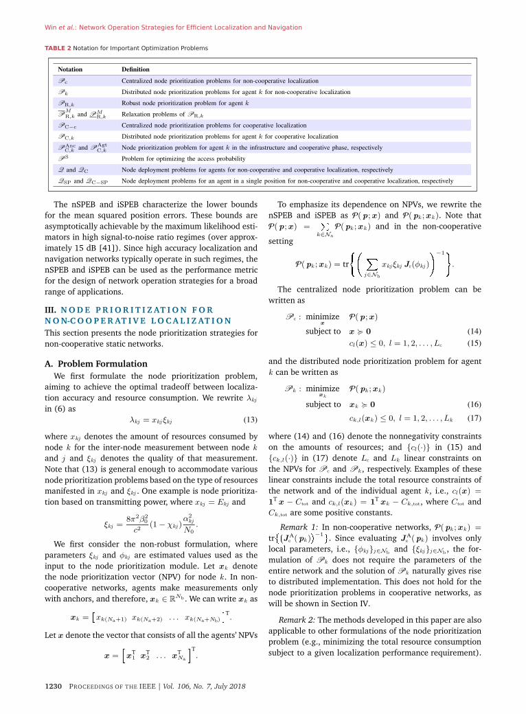
the notation for important quantities and optimization
problems that is used throughout the paper is summarized
in Tables 1 and 2, respectively.
II. P R E L I M I N A R I E S
This section presents the system model in an NLN scenario,
explains basic concepts, and introduces the performance
metric of the network operation.
1226 PROCEEDINGS OF THE IEEE | Vol. 106, No. 7, July 2018
Win et al.: Network Operation Strategies for Efficient Localization and Navigation
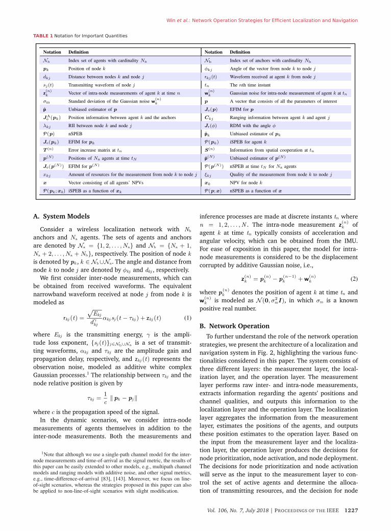
TABLE 1 Notation for Important Quantities
A. System Models
Consider a wireless localization network with Nb
anchors and Na agents. The sets of agents and anchors
are denoted by Na = {1, 2, . . . , Na} and Nb = {Na + 1,
Na + 2, . . . , Na + Nb}, respectively. The position of node k
is denoted by pk , k ∈ Nb∪Na. The angle and distance from
node k to node j are denoted by φkj and dkj , respectively.
We first consider inter-node measurements, which can
be obtained from received waveforms. The equivalent
narrowband waveform received at node j from node k is
modeled as
rkj (t) =
�Ekj
dγkj
αkj sj (t − τkj ) + zkj (t) (1)
where Ekj is the transmitting energy, γ is the ampli-
tude loss exponent, {sj (t)}j∈Nb∪Nais a set of transmit-
ting waveforms, αkj and τkj are the amplitude gain and
propagation delay, respectively, and zkj (t) represents the
observation noise, modeled as additive white complex
Gaussian processes.1 The relationship between τkj and the
node relative position is given by
τkj =1
c‖pk − pj ‖
where c is the propagation speed of the signal.
In the dynamic scenarios, we consider intra-node
measurements of agents themselves in addition to the
inter-node measurements. Both the measurements and
1Note that although we use a single-path channel model for the inter-node measurements and time-of-arrival as the signal metric, the results ofthis paper can be easily extended to other models, e.g., multipath channelmodels and ranging models with additive noise, and other signal metrics,e.g., time-difference-of-arrival [83], [143]. Moreover, we focus on line-of-sight scenarios, whereas the strategies proposed in this paper can alsobe applied to non-line-of-sight scenarios with slight modification.
inference processes are made at discrete instants tn where
n = 1, 2, . . . ,N . The intra-node measurement z(n)k of
agent k at time tn typically consists of acceleration and
angular velocity, which can be obtained from the IMU.
For ease of exposition in this paper, the model for intra-
node measurements is considered to be the displacement
corrupted by additive Gaussian noise, i.e.,
z(n)k = p
(n)k − p
(n−1)k + w
(n)k (2)
where p(n)k denotes the position of agent k at time tn and
w(n)k is modeled as N (0, σ2
mI), in which σm is a known
positive real number.
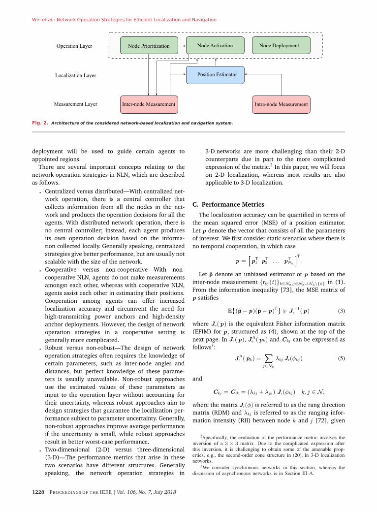
B. Network Operation
To further understand the role of the network operation
strategies, we present the architecture of a localization and
navigation system in Fig. 2, highlighting the various func-
tionalities considered in this paper. The system consists of
three different layers: the measurement layer, the local-
ization layer, and the operation layer. The measurement
layer performs raw inter- and intra-node measurements,
extracts information regarding the agents’ positions and
channel qualities, and outputs this information to the
localization layer and the operation layer. The localization
layer aggregates the information from the measurement
layer, estimates the positions of the agents, and outputs
these position estimates to the operation layer. Based on
the input from the measurement layer and the localiza-
tion layer, the operation layer produces the decisions for
node prioritization, node activation, and node deployment.
The decisions for node prioritization and node activation
will serve as the input to the measurement layer to con-
trol the set of active agents and determine the alloca-
tion of transmitting resources, and the decision for node
Vol. 106, No. 7, July 2018 | PROCEEDINGS OF THE IEEE 1227
Win et al.: Network Operation Strategies for Efficient Localization and Navigation
Fig. 2. Architecture of the considered network-based localization and navigation system.
deployment will be used to guide certain agents to
appointed regions.
There are several important concepts relating to the
network operation strategies in NLN, which are described
as follows.
� Centralized versus distributed—With centralized net-
work operation, there is a central controller that
collects information from all the nodes in the net-
work and produces the operation decisions for all the
agents. With distributed network operation, there is
no central controller; instead, each agent produces
its own operation decision based on the informa-
tion collected locally. Generally speaking, centralized
strategies give better performance, but are usually not
scalable with the size of the network.
� Cooperative versus non-cooperative—With non-
cooperative NLN, agents do not make measurements
amongst each other, whereas with cooperative NLN,
agents assist each other in estimating their positions.
Cooperation among agents can offer increased
localization accuracy and circumvent the need for
high-transmitting power anchors and high-density
anchor deployments. However, the design of network
operation strategies in a cooperative setting is
generally more complicated.
� Robust versus non-robust—The design of network
operation strategies often requires the knowledge of
certain parameters, such as inter-node angles and
distances, but perfect knowledge of these parame-
ters is usually unavailable. Non-robust approaches
use the estimated values of these parameters as
input to the operation layer without accounting for
their uncertainty, whereas robust approaches aim to
design strategies that guarantee the localization per-
formance subject to parameter uncertainty. Generally,
non-robust approaches improve average performance
if the uncertainty is small, while robust approaches
result in better worst-case performance.
� Two-dimensional (2-D) versus three-dimensional
(3-D)—The performance metrics that arise in these
two scenarios have different structures. Generally
speaking, the network operation strategies in
3-D networks are more challenging than their 2-D
counterparts due in part to the more complicated
expression of the metric.2 In this paper, we will focus
on 2-D localization, whereas most results are also
applicable to 3-D localization.
C. Performance Metrics
The localization accuracy can be quantified in terms of
the mean squared error (MSE) of a position estimator.
Let p denote the vector that consists of all the parameters
of interest. We first consider static scenarios where there is
no temporal cooperation, in which case
p =�p
T1 p
T2 . . . p
TNa
�T.
Let p denote an unbiased estimator of p based on the
inter-node measurement {rkj (t)}k∈Na,j∈Na∪Nb\{k} in (1).
From the information inequality [73], the MSE matrix of
p satisfies
E�(p − p)(p − p)T�
� J−1e (p) (3)
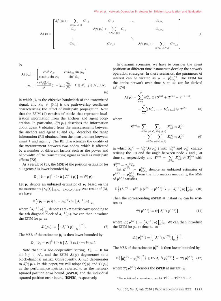
where Je(p) is the equivalent Fisher information matrix
(EFIM) for p, structured as (4), shown at the top of the
next page. In Je(p), J Ae (pk ) and Ckj can be expressed as
follows3:
JAe (pk ) =
�j∈Nb
λkj Jr(φkj ) (5)
and
Ckj = Cjk = (λkj + λjk ) Jr(φkj ) k , j ∈ Na
where the matrix Jr(φ) is referred to as the rang direction
matrix (RDM) and λkj is referred to as the ranging infor-
mation intensity (RII) between node k and j [72], given
2Specifically, the evaluation of the performance metric involves theinversion of a 3 × 3 matrix. Due to the complicated expression afterthis inversion, it is challenging to obtain some of the amenable prop-erties, e.g., the second-order cone structure in (20), in 3-D localizationnetworks.
3We consider synchronous networks in this section, whereas thediscussion of asynchronous networks is in Section III-A.
1228 PROCEEDINGS OF THE IEEE | Vol. 106, No. 7, July 2018
Win et al.: Network Operation Strategies for Efficient Localization and Navigation
Je(p) =
������������
J Ae
(p1) +�
j∈Na\{1}
C1,j −C1,2 . . . −C1,Na
−C2,1 J Ae
(p2) +�
j∈Na\{2}
C2,j −C2,Na
.
.
.. . .
−CNa,1 −CNa,2 J Ae
(pNa) +
�j∈Na\{Na}
CNa,j
������������
(4)
by
Jr(φkj ) =
�cos2 φkj cos φkj sin φkj
cos φkj sin φkj sin2 φkj
�
λkj =8π2β2
0Ekj
c2(1 − χkj )
α2kj
N0k ∈ Na, j ∈ Na ∪Nb
(6)
in which β0 is the effective bandwidth of the transmitted
signal, and χkj ∈ [0, 1] is the path-overlap coefficient
characterizing the effect of multipath propagation. Note
that the EFIM (4) consists of blocks that represent local-
ization information from the anchors and agent coop-
eration. In particular, J Ae (pk ) describes the information
about agent k obtained from the measurements between
the anchors and agent k ; and Ck,j describes the range
information (RI) obtained from the measurement between
agent k and agent j . The RII characterizes the quality of
the measurement between two nodes, which is affected
by a number of different factors such as the power and
bandwidth of the transmitting signal as well as multipath
effects [72].
As a result of (3), the MSE of the position estimator for
all agents p is lower bounded by
E�‖p − p‖2
�≥ tr
�J
−1e (p)
�=: P(p).
Let pk denote an unbiased estimator of pk based on the
measurements {rkj (t)}k∈Na,j∈Na∪Nb\{k}. As a result of (3),
we have
E�(pk − pk )(pk − pk)
T��J
−1e (p)
pk
whereJ−1
e (p)pk
denotes a 2×2 matrix corresponding to
the k th diagonal block of J−1e (p). We can then introduce
the EFIM for pk as
Je(pk ) :=�
J−1e (p)
pk
�−1
. (7)
The MSE of the estimator pk is then lower bounded by
E�‖pk − pk‖2 � ≥ tr
�J
−1e (pk)
�=: P(pk ).
Note that in a non-cooperative setting, Ckj = 0 for
all k , j ∈ Na, and the EFIM Je(p) degenerates to a
block-diagonal matrix. Consequently, Je(pk ) degenerates
to J Ae (pk ). In this paper, we will adopt P(p) and P(pk )
as the performance metrics, referred to as the network
squared position error bound (nSPEB) and the individual
squared position error bound (iSPEB), respectively.
In dynamic scenarios, we have to consider the agent
positions at different time instances to develop the network
operation strategies. In these scenarios, the parameter of
interest can be written as p = p(1:N)1:Na
. The EFIM for
the entire network over time t1 to tN can be derived
as4 [74]
Je(p) =
N�n=1
ENn,n ⊗ (S (n) + T
(n) + T(n+1))
−N�
n=1
(ENn,n+1 + E
Nn+1,n) ⊗ T
(n)(8)
where
S(n)=
�k∈Na
�j∈Na∪Nb\{k}
ENa
k,k ⊗ S(n)kj
−�k∈Na
�j∈Na\{k}
ENa
k,j ⊗ S(n)kj (9)
in which S(n)kj = λ
(n)kj Jr(φ
(n)kj ) with λ
(n)kj and φ
(n)kj charac-
terizing the RII and the angle between node k and j at
time tn, respectively, and T (n) =
k∈Na
ENa
k,k ⊗ T(n)k with
T(n)k = σ−2
m I2.
Let p(N) := p(N)1:Na
denote an unbiased estimator of
p(N) := p(N)1:Na
. From the information inequality, the MSE
of p(N) satisfies
E
�(p(N) − p
(N))(p(N) − p(N))T
��J
−1e (p)
−1
p(N) . (10)
Then the corresponding nSPEB at instant tN can be writ-
ten as
P(p(N)) := tr�J
−1e (p(N))
�(11)
where Je(p(N)) :=
J−1
e (p)−1
p(N) . We can then introduce
the EFIM for pk at time tN as
Je(p(N)k ) =
�J
−1e (p(N))
pk
�−1
.
The MSE of the estimator p(N)k is then lower bounded by
E���p(N)
k − p(N)k
��2� ≥ tr�J
−1e (p
(N)k )
�=: P(p
(N)k ) (12)
where P(p(N)k ) denotes the iSPEB at instant tN .
4For notational convenience, we let T (1) = T (N+1) = 0.
Vol. 106, No. 7, July 2018 | PROCEEDINGS OF THE IEEE 1229
Win et al.: Network Operation Strategies for Efficient Localization and Navigation
TABLE 2 Notation for Important Optimization Problems
The nSPEB and iSPEB characterize the lower bounds
for the mean squared position errors. These bounds are
asymptotically achievable by the maximum likelihood esti-
mators in high signal-to-noise ratio regimes (over approx-
imately 15 dB [41]). Since high accuracy localization and
navigation networks typically operate in such regimes, the
nSPEB and iSPEB can be used as the performance metric
for the design of network operation strategies for a broad
range of applications.
III. N O D E P R I O R I T I Z AT I O N F O R
N O N-C O O P E R AT I V E L O C A L I Z AT I O N
This section presents the node prioritization strategies for
non-cooperative static networks.
A. Problem Formulation
We first formulate the node prioritization problem,
aiming to achieve the optimal tradeoff between localiza-
tion accuracy and resource consumption. We rewrite λkj
in (6) as
λkj = xkj ξkj (13)
where xkj denotes the amount of resources consumed by
node k for the inter-node measurement between node k
and j and ξkj denotes the quality of that measurement.
Note that (13) is general enough to accommodate various
node prioritization problems based on the type of resources
manifested in xkj and ξkj . One example is node prioritiza-
tion based on transmitting power, where xkj = Ekj and
ξkj =8π2β2
0
c2(1 − χkj )
α2kj
N0.
We first consider the non-robust formulation, where
parameters ξkj and φkj are estimated values used as the
input to the node prioritization module. Let xk denote
the node prioritization vector (NPV) for node k . In non-
cooperative networks, agents make measurements only
with anchors, and therefore, xk ∈ RNb . We can write xk as
xk =xk(Na+1) xk(Na+2) . . . xk(Na+Nb)
T.
Let x denote the vector that consists of all the agents’ NPVs
x =�x
T1 x
T2 . . . x
TNa
�T.
To emphasize its dependence on NPVs, we rewrite the
nSPEB and iSPEB as P(p; x) and P(pk ; xk ). Note that
P(p; x) =
k∈Na
P(pk ; xk ) and in the non-cooperative
setting
P(pk ; xk ) = tr
�� �j∈Nb
xkj ξkj Jr(φkj )
�−1�.
The centralized node prioritization problem can be
written as
Pc : minimizex
P(p; x)
subject to x � 0 (14)
cl(x) ≤ 0, l = 1, 2, . . . , Lc (15)
and the distributed node prioritization problem for agent
k can be written as
Pk : minimizexk
P(pk ; xk )
subject to xk � 0 (16)
ck,l(xk ) ≤ 0, l = 1, 2, . . . , Lk (17)
where (14) and (16) denote the nonnegativity constraints
on the amounts of resources; and {cl(·)} in (15) and
{ck,l(·)} in (17) denote Lc and Lk linear constraints on
the NPVs for Pc and Pk , respectively. Examples of these
linear constraints include the total resource constraints of
the network and of the individual agent k , i.e., cl(x) =
1T x − Ctot and ck,l(xk ) = 1
T xk − Ck,tot, where Ctot and
Ck,tot are some positive constants.
Remark 1: In non-cooperative networks, P(pk ; xk) =
tr��
J Ae (pk )
�−1�. Since evaluating J A
e (pk ) involves only
local parameters, i.e., {φkj}j∈Nband {ξkj}j∈Nb
, the for-
mulation of Pk does not require the parameters of the
entire network and the solution of Pk naturally gives rise
to distributed implementation. This does not hold for the
node prioritization problems in cooperative networks, as
will be shown in Section IV.
Remark 2: The methods developed in this paper are also
applicable to other formulations of the node prioritization
problem (e.g., minimizing the total resource consumption
subject to a given localization performance requirement).
1230 PROCEEDINGS OF THE IEEE | Vol. 106, No. 7, July 2018
Win et al.: Network Operation Strategies for Efficient Localization and Navigation
In particular, one can consider a broadcast setting, in which
only anchors are required to transmit signals, and each of
the agents can use the received waveform for ranging. In
this setting, the NPV xb ∈ RNb and its k th element xk
refers to the amount of resources for the wireless signals
broadcast by anchor k . The RII can then be written as
λkj = xkξkj�Nb(k)�Na
(j). (18)
Here, it is more reasonable to select nSPEB P(p; xb) as the
performance metric and the optimization problem is then
minimizex
P(p; xb)
subject to xb � 0
cl(xb) ≤ 0, l = 1, 2, . . . , Lc.
This problem has a similar structure to Pc and Pk , but
it optimizes the resources broadcast by anchors, whereas
Pc and Pk optimize the resources used in point-to-point
measurements. The techniques that will be introduced
in Section III-B can be easily used for this optimization
problem in the broadcast setting because it has a structure
similar to Pc and Pk .
The considered problems Pc and Pk can address the
synchronous case as well as the asynchronous case with
only a slight modification. In particular, consider that
anchors and agents are not synchronized. A feasible local-
ization method in this case uses round-trip ranging: node
k initiates by transmitting a wireless signal to node j ,
and node j responds by transmitting a wireless signal
back to node k ; the range dkj is inferred at node k from
the round trip time. Let λjk and xjk denote the RII and
the resource of the response signal sent from node j
to node k , respectively. The matrix J Ae (pk ) can then be
expressed as
JAe (pk ) =
�j∈Nb
4λkj λjk
λkj + λjk
Jr(φkj )
=�j∈Nb
4xkj xjk
xkj + xjk
ξkjJr(φkj )
where the second equality is because of the channel reci-
procity, i.e., ξkj = ξjk . In practice, there are two common
scenarios.
� Highly asymmetric networks—In certain networks
(e.g., cellular networks), the transmitting resources
(e.g., transmitting power) from anchors (e.g., base
stations) are significantly larger than those from
agents (e.g., mobile users) and cannot be controlled
by the agents. In this scenario, the node prioritization
problem is to optimize over {xkj}j∈Nbfor each agent
k with the assumption that xjk ≫ xkj , j ∈ Nb. The
matrix J Ae (pk ) can be approximated as
JAe (pk ) ≈
�j∈Nb
4xkj ξkjJr(φkj )
and has the same structure as (5) with λkj given
in (13).
� Proportional amount of response resources—In cer-
tain scenarios, the amounts of resources for the
response signals are proportional to those for the
initiating signals, i.e., xjk = ηxkj , where η ∈ R+
does not depend on k or j .5 With this resource allo-
cation method, the node prioritization problem is to
optimize over {xkj }j∈Nbfor each agent k with the
assumption that xjk = ηxkj , j ∈ Nb. The matrix
J Ae (pk ) becomes
JAe (pk ) =
�j∈Nb
4η
1 + ηxkj ξkjJr(φkj )
and has the same structure as (5) with λkj given
in (13).
For readers who are interested in the node prioritization
strategies in asynchronous networks, see [88]–[90] for a
more detailed discussion.
B. Conic Programming-Based Approaches
We next provide solutions to the node prioritization
problems Pc and Pk with conic programming-based
approaches. Note that if there is only one agent in the
network, Pc degenerates to Pk . Therefore, Pk can be
seen as a special case of Pc, and we will focus our attention
on Pc in the following.
Proposition 1 (Convexity): The nSPEB P(p; x) in non-
cooperative networks is convex in x � 0.
There are many ways to prove Proposition 1, where the
details can be found in [142]–[144]. One way is to take the
second derivative of P(p; x) with respect to x and show
that the Hessian matrix is positive semidefinite [144].
Proposition 1 shows that the objective function of Pc
is convex in x. Thus, together with the fact that P has
convex constraints, Proposition 1 implies that Pc is a
convex program [146]–[148]. Consequently, the optimal
solution can be obtained numerically by standard convex
optimization algorithms [146].
Conic optimization is a special type of convex optimiza-
tion, and it includes the most well-known classes of con-
vex optimization problems such as semidefinite programs
(SDPs) and SOCPs. We next show that Pc can be converted
to an SDP, which is a more favorable formulation than the
general convex formulation. Recall that the nSPEB can be
written as
P(p; x) = tr��
Je(p)�−1�
=�
k∈Nb
tr��
JAe (pk )
�−1�.
Let us consider an auxiliary matrix Mk with the following
constraint:
Mk ��J
Ae (pk )
�−1.
Due to the fact that J Ae (pk ) � 0, the constraint above can
be equivalently transformed to the semidefiniteness of a
matrix that involves Mk and xk , as shown in the following
5This allocation for the response signals is shown to be optimal inthe scenario with certain resource constraints [142], and it has beenimplemented in practice [117].
Vol. 106, No. 7, July 2018 | PROCEEDINGS OF THE IEEE 1231

Win et al.: Network Operation Strategies for Efficient Localization and Navigation
proposition. A detailed proof of Proposition 2 can be found
in [142].
Proposition 2 (SDP): The problem Pc is equivalent to
the SDP
minimizex,{Mk}k∈N
b
�k∈Na
tr{Mk}
subject to
��Mk I
I
j∈Nb
xkj ξkj Jr(φkj )
�� � 0, ∀k ∈ Na
(14) − (15).
Furthermore, the problem Pc can also be converted
to an SOCP problem, which is an even more favorable
formulation than the SDP formulation. To see how we
can achieve this, we first transform Pc to the following
problem:
minimizex,{k}k∈N
b
�k∈Nb
k
subject to P(pk ; xk) ≤ k , ∀k ∈ Na
(14) − (15).
To transform the constraint P(pk ; xk) ≤ k to a desired
form, we next explicitly rewrite the iSPEB as follows:
P(pk ; xk ) =4 · 1TRk xk
xTk RT
k (11T − ck cT
k − sk sTk )Rk xk
(19)
where
Rk = diag�ξk(Na+1), ξk(Na+2), . . . , ξk(Na+Nb)
�and
ck =
cos 2φk(Na+1) cos 2φk(Na+2) . . . cos 2φk(Na+Nb)
Tsk =
sin 2φk(Na+1) sin 2φk(Na+2) . . . sin 2φk(Na+Nb)
T.
The constraint P(pk ; xk) ≤ k can then be transformed
into ��� cTk yk s
Tk yk 2tk
T��� ≤ 1Tyk − 2tk (20)
where yk = Rk xk and tk = 1/k . The constraint tk =
1/k can be replaced with the following constraint without
changing the optimal solution:��� tk k
√2T��� ≤ tk + k .
We then have the following proposition. A detailed proof
of Proposition 3 can be found in [143].
Proposition 3 (SOCP): The problem Pc is equivalent to
the SOCP
minimizex,{tk ,k}k∈Na
�k∈Na
k
subject to ‖AkRkxk + bk‖ ≤ 1TRkxk − 2tk , ∀k ∈ Na��� tk k
√2T��� ≤ tk + k , ∀k ∈ Na
(14) − (15)
where Ak = [ ck sk 0 ]T and bk = [ 0 0 2tk ]T.
Remark 3: Regarding the computational complex-
ity, the worst-case running time of both the SDP- and
SOCP-based approaches is O(Nb
3.5) for the single-agent
case [149].
C. Computational Geometry-Based Approaches
While conic programming-based approaches can pro-
vide solutions with amenable complexity, those solutions
are ǫ-approximate numerical ones and limited insight into
the problem can be gained from the numerical solutions.
We next present another type of approach, which not only
provides exact solutions to the problem, but also reveals
the essence of node prioritization problems.
In this section, we consider that the NPVs are sub-
ject to nonnegative constraints, i.e., (14) and (16), and
the total resource constraints, i.e., (15) with Lc = 1
and c1(x) = 1T x − 1, and (17) with Lk = 1 and
ck,1 = 1T xk − 1. This is a common scenario in the
design and implementation of a localization and naviga-
tion system. For example, the amount of available time for
ranging with different anchors is subject to a total time
constraint.
We next formulate a geometric framework, under which
we can obtain solutions of Pk , and then adopt these
solutions to solve Pc.
1) Geometric Framework: Inspired by the structure
in (19), we introduce an affine transformation that maps
an NPV to a point in 3-D space
zk = Ckxk (21)
where Ck = [ ck sk 1 ]TRk . With this transformation, the
iSPEB can be written as
Q(zk) :=4[zk ]3
[zk ]23 − [zk ]21 − [zk ]22= P(pk ; xk ).
This leads to the following geometric interpretation of the
iSPEB. Given an NPV xk , the point zk = Ckxk lies on a
hyperboloid, given by
(z3 − 2η−1)2 − z21 − z2
2 − 4η−2 = 0 (22)
where z1, z2, and z3 are variables and η = P(pk ; xk).
Denote the feasible NPV set of Pk and its image set
under the transformation (21), respectively, by
Xk = {xk ∈ RNb : 1T
xk = 1,0 � xk}
and
Zk = {zk ∈ RNb : zk = Ckxk , xk ∈ Xk}.
Note that each element xk ∈ Xk can be written as a
convex combination of elements in E := {e1, e2, . . . , eNb},
where ek is a unit vector with the k th element being 1
and all other elements being 0’s. Hence, the image set
Zk is a convex polyhedron, given by Hc{Cke : e ∈ E}.
This implies that for xk ∈ Xk with the corresponding
iSPEB P(pk ; xk ), Ckxk is in the intersection of Zk and the
1232 PROCEEDINGS OF THE IEEE | Vol. 106, No. 7, July 2018
Win et al.: Network Operation Strategies for Efficient Localization and Navigation
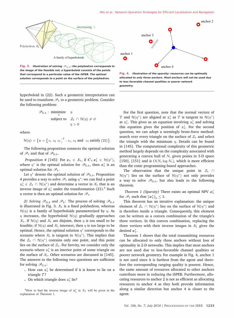
Fig. 3. Illustration of solving PG,k : the polyhedron corresponds to
the image of the feasible set; a hyperboloid consists of the points
that correspond to a particular value of the iSPEB. The optimal
solution corresponds to a point on the surface of the polyhedron.
hyperboloid in (22). Such a geometric interpretation can
be used to transform Pk to a geometric problem. Consider
the following problem:
PG,k : minimizeη
η
subject to Zk ∩ H(η) �= ∅
η > 0
where
H(η) =�z =
z1 z2 z3
T: z1, z2 and z3 satisfy (22)
�.
The following proposition connects the optimal solution
of Pk and that of PG,k.
Proposition 4 [145]: For xk ∈ Xk , if Ck x∗k ∈ H(η∗),
where η∗ is the optimal solution for PG,k, then x∗k is an
optimal solution for Pk .
Let η∗ denote the optimal solution of PG,k. Proposition
4 provides a way to solve Pk using η∗: we can find a point
z∗k ∈ Zk ∩ H(η∗) and determine a vector in Xk that is an
inverse image of z∗k under the transformation (21).6 Such
a vector is then an optimal solution for Pk .
2) Solving PG,k and Pk : The process of solving PG,k
is illustrated in Fig. 3. Xk is a fixed polyhedron, whereas
H(η) is a family of hyperboloids parameterized by η. As
η increases, the hyperboloid H(η) gradually approaches
Xk . If H(η) and Xk are disjoint, then η is too small to be
feasible; if H(η) and Xk intersect, then η is too large to be
optimal. Hence, the optimal solution η∗ corresponds to the
scenario where Xk is tangent to H(η∗). This implies that
the Zk ∩ H(η∗) contains only one point, and this point
lies on the surface of Zk . For brevity, we consider only the
scenario where z∗k is an interior point of some triangle on
the surface of Xk . Other scenarios are discussed in [145].
The answers to the following two questions are sufficient
for solving PG,k:
� How can z∗k be determined if it is know to lie on a
triangle T ?
� On which triangle does z∗k lie?
6How to find the inverse image of z∗k
in Xk will be given in theexplanation of Theorem 1.
Fig. 4. Illustration of the sparsity: resources can be optimally
allocated to only three anchors. Most anchors will not be used due
to less favorable channel qualities or poorer network
geometry.
For the first question, note that the normal vectors of
T and H(η∗) are aligned at z∗k as T is tangent to H(η∗)
at z∗k . This gives us an equation involving z∗
k and solving
this equation gives the position of z∗k . For the second
question, we can adopt a seemingly brute-force method:
search over every triangle on the surface of Zk and select
the triangle with the minimum η. Details can be found
in [145]. The computational complexity of this geometric
method largely depends on the complexity associated with
generating a convex hull of Nb given points in 3-D space
[150], [151] and is O(Nb log Nb), which is more efficient
than the conic programming-based approaches.
The observation that the unique point in Zk ∩H(η∗) lies on the surface of H(η∗) not only provides
a way to solve PG,k, but also leads to the following
theorem.
Theorem 1 (Sparsity) There exists an optimal NPV x∗k
for Pk such that ‖x∗k‖0 ≤ 3.
This theorem has an intuitive explanation: the unique
element of Zk ∩ H(η∗) lies on the surface of H(η∗) and
is therefore inside a triangle. Consequently, this element
can be written as a convex combination of the triangle’s
three vertices. In this convex combination, replacing the
three vertices with their inverse images in Xk gives the
desired x∗k .
Theorem 1 shows that the total transmitting resources
can be allocated to only three anchors without loss of
optimality in 2-D networks. This implies that most anchors
are not used due to less-favorable channel qualities or
poorer network geometry. For example in Fig. 4, anchor 1
is not used since it is farthest from the agent and there-
fore the corresponding ranging quality is poorest. Hence,
the same amount of resources allocated to other anchors
contribute more in reducing the iSPEB. Furthermore, allo-
cating resources to anchor 2 is not as efficient as allocating
resources to anchor 4 as they both provide information
along a similar direction but anchor 4 is closer to the
agent.
Vol. 106, No. 7, July 2018 | PROCEEDINGS OF THE IEEE 1233
Win et al.: Network Operation Strategies for Efficient Localization and Navigation
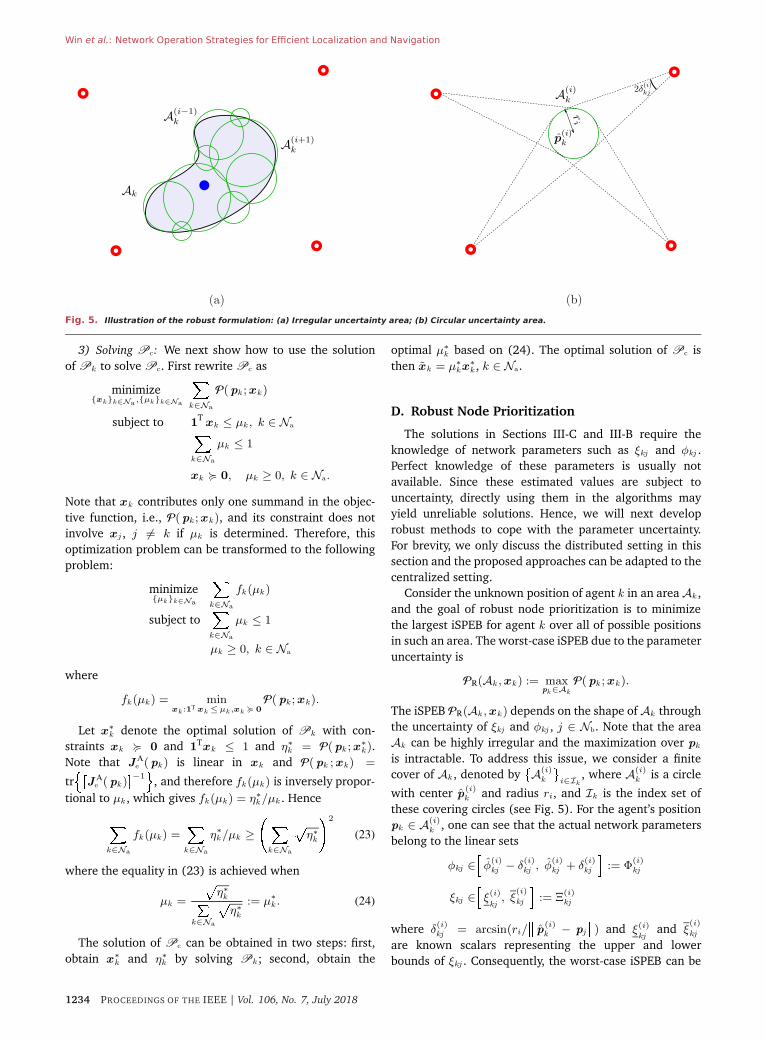
Fig. 5. Illustration of the robust formulation: (a) Irregular uncertainty area; (b) Circular uncertainty area.
3) Solving Pc: We next show how to use the solution
of Pk to solve Pc. First rewrite Pc as
minimize{xk}k∈Na
,{µk}k∈Na
�k∈Na
P(pk ; xk )
subject to 1Txk ≤ μk , k ∈ Na�
k∈Na
μk ≤ 1
xk � 0, μk ≥ 0, k ∈ Na.
Note that xk contributes only one summand in the objec-
tive function, i.e., P(pk ; xk ), and its constraint does not
involve xj , j �= k if μk is determined. Therefore, this
optimization problem can be transformed to the following
problem:
minimize{µk}k∈Na
�k∈Na
fk (μk )
subject to�k∈Na
μk ≤ 1
μk ≥ 0, k ∈ Na
where
fk (μk ) = minxk :1T xk ≤ µk ,xk � 0
P(pk ; xk).
Let x∗k denote the optimal solution of Pk with con-
straints xk � 0 and 1Txk ≤ 1 and η∗
k = P(pk ; x∗k ).
Note that J Ae (pk ) is linear in xk and P(pk ; xk) =
tr�
J Ae (pk )
−1�
, and therefore fk (μk ) is inversely propor-
tional to μk , which gives fk (μk ) = η∗k /μk . Hence
�k∈Na
fk (μk) =�k∈Na
η∗k /μk ≥
��k∈Na
�η∗k
�2
(23)
where the equality in (23) is achieved when
μk =
�η∗k
k∈Na
�η∗k
:= μ∗k . (24)
The solution of Pc can be obtained in two steps: first,
obtain x∗k and η∗
k by solving Pk ; second, obtain the
optimal μ∗k based on (24). The optimal solution of Pc is
then xk = μ∗kx∗
k , k ∈ Na.
D. Robust Node Prioritization
The solutions in Sections III-C and III-B require the
knowledge of network parameters such as ξkj and φkj .
Perfect knowledge of these parameters is usually not
available. Since these estimated values are subject to
uncertainty, directly using them in the algorithms may
yield unreliable solutions. Hence, we will next develop
robust methods to cope with the parameter uncertainty.
For brevity, we only discuss the distributed setting in this
section and the proposed approaches can be adapted to the
centralized setting.
Consider the unknown position of agent k in an area Ak ,
and the goal of robust node prioritization is to minimize
the largest iSPEB for agent k over all of possible positions
in such an area. The worst-case iSPEB due to the parameter
uncertainty is
PR(Ak , xk ) := maxpk∈Ak
P(pk ; xk ).
The iSPEB PR(Ak , xk ) depends on the shape of Ak through
the uncertainty of ξkj and φkj , j ∈ Nb. Note that the area
Ak can be highly irregular and the maximization over pk
is intractable. To address this issue, we consider a finite
cover of Ak , denoted by�A(i)
k
�i∈Ik
, where A(i)k is a circle
with center p(i)k and radius ri, and Ik is the index set of
these covering circles (see Fig. 5). For the agent’s position
pk ∈ A(i)k , one can see that the actual network parameters
belong to the linear sets
φkj ∈�φ
(i)kj − δ
(i)kj , φ
(i)kj + δ
(i)kj
�:= Φ
(i)kj
ξkj ∈�ξ(i)
kj, ξ
(i)
kj
�:= Ξ
(i)kj
where δ(i)kj = arcsin(ri/
�� p(i)k − pj
��) and ξ(i)
kjand ξ
(i)
kj
are known scalars representing the upper and lower
bounds of ξkj . Consequently, the worst-case iSPEB can be
1234 PROCEEDINGS OF THE IEEE | Vol. 106, No. 7, July 2018
Win et al.: Network Operation Strategies for Efficient Localization and Navigation
bounded by
PR(Ak , xk ) ≤ maxi∈Ik
P(i)R (Ak , xk)
where
P(i)R (Ak , xk) := max
φkj∈Φ(i)kj
,ξkj∈Ξ(i)kj
P(pk ; xk ). (25)
We can then formulate the robust node prioritization
problem as
PR,k : minimizexk
maxi∈Ik
P(i)R (Ak , xk)
subject to (16) − (17)
which can be equivalently transformed into
minimizexk,t
t
subject to P(i)R (Ak , xk ) ≤ t, ∀i ∈ Ik
(16) − (17). (26)
We need to convert P(i)R (Ak , xk ) into an expression
amenable to efficient optimization. Note that in (25), the
maximization over ξkj is achieved at ξkj = ξ(i)
kjsince the
iSPEB P(pk ; xk ) is a monotonically decreasing function in
ξkj . However, maximization over φkj is nontrivial. We next
provide upper bounds on P(i)R (Ak , xk) that lead to conic
programming solutions.
Proposition 5 ([142]) The maximum iSPEB over the
actual angle φkj is upper bounded by
P(i)R (Ak , xk) ≤ tr
���j∈Nb
xkj ξ(i)
kjQ
r(φ
(i)kj , δ
(i)kj )
�−1�(27)
provided that
j∈Nb
xkj ξ(i)
kjQ
r(φ
(i)kj , δ
(i)kj ) � 0, where
Qr(φ
(i)kj , δ
(i)kj ) = Jr(φ
(i)kj ) − sin δ
(i)kj I .
Proposition 5 can be proved by noting that if φkj ∈ Φ(i)kj ,
Jr(φkj ) � Qr(φ
(i)kj , δ
(i)kj )
and thus
JAe (pk ) =
�j∈Nb
xkj ξkjJr(ϕkj ) ��j∈Nb
xkj ξ(i)
kjQ
r(φ
(i)kj , δ
(i)kj ).
This together with the monotonicity of tr{(·)−1} completes
the proof. Replacing P(i)R (Ak , xk) in (26) with its upper
bound in (27) and adopting a similar transformation as in
Proposition 2, we can relax the robust node prioritization
problem PR,k into the following SDP:
minimizex,{Mi}i∈Ik
t
subject to tr{Mi} ≤ t, i ∈ Ik��Mi I
I
j∈Nb
xkj ξ(i)
kjQ
r(φ
(i)kj , δ
(i)kj )
�� � 0,
i ∈ Ik
(16) − (17).
The above SDP can cope with small uncertainty in
the parameters. However, the performance loss from the
relaxation is difficult to quantify since the optimal solution
of the robust formulation remains unknown. To address
this issue, we look for new bounds of the worst-case iSPEB.
We denote M = {0, 1, . . . , M − 1}, where M ∈ Z.
Proposition 6 ([143]) For any given NPV xk such that
P(i)R (Ak ; xk ) < ∞, if
M ≥ π
2
�P
(i)R (Ak , xk ) · 1TR
(i)k xk
where R(i)k = diag
�ξ(i)
k(Na+1), ξ(i)
k(Na+2), . . . , ξ(i)
k(Na+Nb)
�,
then P(i)R (Ak , xk ) is bounded below and above,
respectively, by
P(i)M (Ak ; xk )= max
m∈M
4 · 1T R(i)k xk
(1T R(i)k xk )2 −
�h
(i) Tk,m R
(i)k xk
�2 (28)
P(i)M (Ak ; xk )= max
m∈M
4 · 1T R(i)k xk
(1T R(i)k xk )2 −
�g
(i) Tk,m R
(i)k xk
�2 (29)
where h(i)k,m, g
(i)k,m ∈ R
Nb , in which their j th elements are
given by �h
(i)k,m
�j= max
|ǫ|≤2δ(i)kj
cos(2φ(i)kj − ϑm + ǫ)
�g
(i)k,m
�j=
1
cos(π/M)·�h
(i)k,m
�j
with ϑm = (2m + 1)π/M for m ∈ M.
Unlike Proposition 5, Proposition 6 provides both lower
and upper bounds for P(i)R (Ak , xk). We can replace
P(i)R (Ak , xk ) in (26) by the lower and upper bounds (28)
and (29), leading to the relaxed problems PMR,k and P
M
R,k,
respectively. PM
R,k is more desirable since it guarantees the
worst-case performance, whereas the lower bound is useful
to bound the performance loss of such relaxation. Note that
the relaxed constraint P(i)M (Ak ; xk) ≤ t can be transformed
into M second-order cone forms of xk . Consequently, PM
R,k
can be transformed into an SOCP as follows:
minimizexk ,y
− y
subject to���A(i)
k,mR(i)k xk + bk
��� ≤ 1TR
(i)k xk − 2y,
∀m ∈ M, ∀i ∈ Ik
(16) − (17)
where A(i)k,m =
g
(i)k,m 0
Tand bk = [ 0 2y ]T.
The next proposition shows that the solution of the
relaxed problem PM
R,k converges to that of the original
problem PR,k as M increases.
Proposition 7 [143] Let x∗k and xM
k be the optimal
solutions of PR,k and PM
R,k, respectively. Then
P(i)R (Ak ; x
Mk )
1 + CM
≤ P(i)R (Ak ; x
∗k ) ≤ P(i)
R (Ak ; xMk )
Vol. 106, No. 7, July 2018 | PROCEEDINGS OF THE IEEE 1235
Win et al.: Network Operation Strategies for Efficient Localization and Navigation
where
CM = maxi∈Ik
sin2(π/M)[Bi(x∗k ) − 1]
1 − sin2(π/M)Bi(x∗k)
in which
Bi(xk) =1
4P
(i)R (Ak , xk) · 1T
R(i)k xk .
Moreover, CM converges to zero at the rate
of O(M−2).
Proposition 7 implies that the optimal solution of PM
R,k
can approximate PR,k with a small value of M due
to the fast convergence rate O(M−2). Consequently, the
performance of the proposed SOCP algorithms can achieve
near-optimal performance with negligible increase in com-
putational complexity.
IV. N O D E P R I O R I T I Z AT I O N F O R
C O O P E R AT I V E L O C A L I Z AT I O N
This section presents the node prioritization strategies for
cooperative networks in static scenarios. In this section, we
consider only the non-robust formulation for brevity. The
techniques developed in Section III-D can be adopted to
address the robust formulation as shown in [84] and [85].
A. Problem Formulation
Similarly to Section III-A, we rewrite λkj as in (13).
In cooperative networks, agents make measurements only
with anchors and agents, and therefore, the NPV for node
k xk ∈ RNa+Nb−1 can be written as
xk =xk1 xk2 . . . xk(k−1) xk(k+1) . . . xk(Nb+Na)
T
and the NPV for all the agents x can be written as
x =�x
T1 x
T2 . . . x
TNa
�T.
For the centralized and distributed settings, the node
prioritization problem can then be written, respectively,
as
PC−c : minimizex
P( p; x)
subject to (14) − (15)
and
PC,k : minimizexk
P( pk; xk)
subject to (16) − (17)
where PC−c denotes the cooperative centralized node
prioritization problem and PC,k denotes the cooperative
distributed node prioritization problem for agent k. Unlike
the node prioritization in non-cooperative networks, the
performance metrics P( p; x) and P( pk; xk) incorporate
range information from agents in addition to that from
anchors. As we will see in the following sections, such addi-
tional information makes the node prioritization problem
more complicated.
B. Centralized Setting
We next provide solutions to the cooperative node prior-
itization problem PC−c in the centralized setting.
Proposition 8: The nSPEB P( p; x) in cooperative net-
works is convex in x � 0.
Proposition 8 can be proved in a similar way as Propo-
sition 1. As the result of convexity, the optimal solution
for PC−c can be obtained numerically by standard convex
optimization algorithms [146].
We next show that PC−c can be converted to an SDP.
Note that
Je( p; x) =�
k∈Na
�j∈Na∪Nb\{k}
xkjξkjVkj
where
Vkj =
�ENa
k,k⊗Jr(φkj), j ∈ Nb�ENa
k,k + ENaj,j − ENa
k,j − ENaj,k
�⊗Jr(φkj), j ∈ Na.
Since Je( p; x) is linear in x, we can use the same tech-
nique as used in Section III-B to prove that PC−c is
equivalent to the SDP
minimizex,M
�k∈Na
tr{M}
subject to
��M I
I
k∈Na
j∈Na∪Nb\{k}
xkjξkjVkj
�� � 0
(14) − (15).
Unfortunately, the techniques of transforming node pri-
oritization problems further into SOCPs in non-cooperative
networks cannot be applied here because the off-diagonal
blocks −Cj,k in (4) make the expression of inverted EFIM
J−1e (p; x) complicated [152], and thus it cannot be writ-
ten as the sum of fractional forms as in (19).
C. Distributed Setting
The optimal solutions of the problem PC,k ’s cannot
be obtained in a distributed manner because the iSPEB
P( pk; xk) = tr�
J−1e ( p; x)
pk
�depends on the angles
and qualities of all the inter-node measurements of the
entire network as well as the node prioritization decisions
(i.e., the NPV) of other agents. To address this issue, we
derive an upper bound for P( pk; xk) that is amenable for
distributed implementation.
Consider an auxiliary matrix JLe ( p; x) representing
the measurements between agents and anchors as
well as measurements made from agent 1 to other
agents
JLe ( p; x)=
�k∈Na
�j∈Nb
xkjξkjVkj+�
j∈Na\{1}
x1jξ1jV1j . (30)
Note that
Je( p; x) − JLe (p; x) =
�k∈Na\{1}
�j∈Na\{k}
xkjξkjVkj � 0
1236 PROCEEDINGS OF THE IEEE | Vol. 106, No. 7, July 2018

Win et al.: Network Operation Strategies for Efficient Localization and Navigation
where the inequality is due to the fact that each summand
is positive semidefinite. Based on JLe ( p; x), a lower bound
for the EFIM of agent 1 is shown to be���J
Le ( p; x)
�−1�
p1
�−1
= JAe ( p1) +
�j∈Na\{1}
x1jξ1jJr(φ1j)
1 + x1jξ1j∆1j
:= JLe (p1; x1)
where
∆1j = tr{Jr(φ1j)�J
Ae ( pj)
�−1} (31)
represents the position uncertainty of agent j along
the direction between agent 1 and agent j [85].
Consequently
P( p1; x1) = tr
���Je(p; x)
�−1�
p1
�≤ tr
���J
Le (p; x)
�−1�
p1
�= tr
��J
Le ( p1; x1)
�−1�
. (32)
Similarly, we can obtain JLe ( pk; xk) as the lower bound
for the EFIM of agent k in cooperative networks. Note that
if ∆kj is available to agent k, then JLe ( pk; xk) depends
only on the local network parameters and on the node
prioritization decision of agent k, facilitating the design of
distributed node prioritization strategies.
Using the upper bound in (32) as the optimization
objective for agent 1 requires obtaining ∆1j . Obtaining
∆1j in turn requires the node prioritization decision of
agent j. To circumvent this difficulty, the original problem
can be transformed into a sequential two-phase optimiza-
tion problem. Specifically, each agent k produces its node
prioritization decision through the following two phases:
� infrastructure phase—produce the node prioritization
decision to allocate resources for the measurements
between agent k and the anchors;
� cooperation phase—produce the node prioritization
decision to allocate resources for the measure-
ments between agent k and its neighboring agents,
which have obtained their position knowledge in the
infrastructure phase.
Note that in the infrastructure phase, each agent k min-
imizes tr��
JAe ( pk)
�−1�without requiring the node prior-
itization decisions of other agents; and in the cooperation
phase, each agent k minimizes tr��
JLe ( pk; xk)
�−1�with
∆kj based on JAe ( pj) (j ∈ Na\{k}) from the infrastructure
phase.
In the infrastructure phase, each agent k minimizes
tr��
JAe ( pk; xk)
�−1�with respect to NPV xk with xkj = 0
for all j ∈ Na, i.e.,
PAncC,k : minimize
xk
tr��
JAe ( pk; xk)
�−1�subject to xkj = 0, ∀j ∈ Na
(16) − (17).
Note that PAncC,k is equivalent to Pk and can be solved via
the techniques in Section III.
Using the solution of PAncC,k in the infrastructure phase,
each agent j broadcasts JAe ( pj) to its neighboring agents
and agent k computes ∆kj . The node prioritization prob-
lem for agent k in the cooperation phase is then formu-
lated using the upper bound (32) as relaxed performance
metrics
PAgtC,k : minimize
xk
tr��
JLe ( pk; xk)
�−1�subject to (16) − (17).
We next show that PAgtC,k can be converted to an SOCP.
We rewrite JLe ( pk; xk) as
JLe ( pk; xk) = J
Ae ( pk) +
�j∈Na\{k}
ξkjqkjJr(φkj)
where
qkj =xkj
1 + xkjξkj∆kj
.
Since tr��
JLe (pk; xk)
�−1�is an increasing function of qkj ,
PAgtC,k is equivalent to the following program:
minimizexk,{qkj}j∈Na\{k}
tr
��J
Ae (pk) +
�j∈Na\{1}
ξkjqkjJr(φkj)
�−1�
subject to 0 ≤ qkj , ∀j ∈ Na\{k}qkj ≤ xkj
1 + xkjξkj∆kj
, ∀j ∈ Na\{k} (33)
(16) − (17).
The objective function has a similar structure to (19).
Therefore, it can be shown that we can transform the
objective function to a linear objective function and an
SOCP constraint by following steps similar to those in
Section III-B [85]. Consequently, PAgtC,k can be transformed
into
minimizexk,{qkj}j∈Na\{k}
− t
subject to 0 ≤ qkj , ∀j ∈ Na\{k}���√2 1 − qkjξkj∆kj 1 + qkjξkj∆kj
T���
≤ 2 + (xkj − qkj)ξkj∆kj , ∀j ∈ Na\{k}��� �Ak�Rkqk + �bk
��� ≤ 1T �Rkqk − 2t
(16) − (17)
where �Ak = [ �ck �sk 0 ]T and �bk = [ 0 0 2t ]T, in which
qk =qk(Na+1) qk(Na+2) . . . qk(k−1) qk(k+1) . . .
qk(Na+Nb) 1 1T
�Rk = diag�ξk(Na+1), ξk(Na+2), . . . , ξk(k−1), ξk(k+1), . . . ,
ξk(Na+Nb), ν(1)k , ν
(2)k
��ck =
cos 2φk(Na+1) cos 2φk(Na+2) . . . cos 2φk(k−1)
cos 2φk(k+1) . . . cos 2φk(Na+Nb) cos 2θk − cos 2θk
T
Vol. 106, No. 7, July 2018 | PROCEEDINGS OF THE IEEE 1237
Win et al.: Network Operation Strategies for Efficient Localization and Navigation
�sk =sin 2φk(Na+1) sin 2φk(Na+2) . . . sin 2φk(k−1)
sin 2φk(k+1) . . . sin 2φk(Na+Nb) sin 2θk − sin 2θk
Twith ν
(1)k , ν
(2)k ≥ 0 being the eigenvalues of JA
e (pk) and
u(θk) and u(θk + π/2) being the corresponding eigenvec-
tors, i.e., JAe ( pk) = ν
(1)k Jr(θk) + ν
(2)k Jr(θk + π/2).
The detailed distributed cooperative node prioritization
strategy is described in Algorithm 1. In Algorithm 1, each
agent requires only local network parameters and little
information from its neighbors, which makes the algorithm
amenable for distributed implementation.
Algorithm 1: Distributed Cooperative Node
Prioritization [84]
Input: φkj and ξkj , k ∈ Na, j ∈ Nb ∪Na\{k}Output: xk, k ∈ Na
1: For k ∈ Na, agent k solves PAncC,k in the infrastructure
phase;
2: For k ∈ Na, agent k broadcasts JAe ( pk) to its neigh-
boring agents;
3: For k ∈ Na, agent k solves PAgtC,k in the cooperation
phase;
4: For k ∈ Na, agent k outputs xk;
V. N O D E A C T I VAT I O N
This section presents the node activation strategies for
cooperative dynamic networks. For the sake of collision
avoidance in implementation, only one node is activated
at each time slot to make inter-node measurements, and
the node then allocates its resource for performing mea-
surements with different neighbors based on the node
prioritization strategies discussed in Section IV. We will
also consider a simpler case for which the node merely
selects one neighbor for the inter-node measurement.
A. Activation Formulation
In the dynamic scenario, recall the EFIM Je(p(n)) given
in (10) for all the node positions at time tn. For ease of
discussion, we define the error matrix at time tn as Q(n) =�Je(p(n))
�−1, and {Q(n)}n≥1 denotes an evolution of the
error matrix over time.
With node activation, at each instant tn, one node
kn is selected to make inter-node measurements with its
neighbors and a fraction of resources is used for each
neighbor through for instance spectrum sharing. In this
case, the error evolution {Q(n)}n≥1 can be written as
Q(n+1) = Q
(n) − Γ(n)kn
+ T(n)
(34)
where Γ(n)kn
is the error reduction matrix corresponding
to the inter-node measurements between nodes kn and
its neighbors, and T (n) is the error increase matrix given
in (8) due to the uncertainty in the intra-node measure-
ments. Moreover, let N (n)k be the set of neighbors of node k
at time tn, and then the error reduction matrix can be
derived as
Γ(n)k = Q
(n) −�
(Q(n))−1 +�
j∈N(n)k
λ(n)kj a
(n)kj a
(n) Tkj
�−1
(35)
where λ(n)kj is the RII of the inter-node measurement
between node k and node j [72], and
a(n)kj =
��� ek ⊗ u(φ(n)kj ), k ∈ Na, j ∈ Nb
(ek − ej) ⊗ u(φ(n)kj ), k, j ∈ Na.
(36)
Remark 4: The evolution of the error matrix (34) implies
that a high accuracy in the inter-node measurements (i.e.,
large λ(n)kj ) or intra-node measurements (i.e., small σ2
m)
translates to large Γ(n)k or small T (n), both leading to high
localization accuracy (i.e., small Q(n+1)). Moreover, the
values of RII λ(n)kj ’s for j ∈ N (n)
k are subject to the total
resource constraint, and node prioritization can be applied
to optimize the resource allocation.
The error evolution in (34) depends on the activation
strategy via the selected node kn together with the node
prioritization (or simply neighbor selection) strategy as
well as the error increase due to the nodes’ mobility at
each instant. Comparing this with data networks, we can
view Q(n), Γ (n), and T (n) as the queue length, service,
and the packet arrival, respectively. In contrast to queueing
dynamics where the service rates are commonly indepen-
dent of the queue lengths and network geometry, the error
reduction matrices in NLN are nonlinear functions of the
queue length Q(n) and of the relative node positions, which
are characterized by φ(n)kj ’s and λ
(n)kj ’s.
Node activation strategies for NLN are typically designed
to coordinate the inter-node measurements, with a goal
of minimizing a performance metric such as the nSPEB
tr{Q(n)} at each time tn, or the time-averaged nSPEB over
the first n instants, given by
qn :=1
n
n�n′=1
tr{Q(n′)}. (37)
We next adopt the former as the performance metric for
designing node activation strategies.
Opportunistic activation: The opportunistic activation
algorithm is one-step optimal and it can be described as
follows: it selects the best agent for inter-node measure-
ments with its neighbors, i.e.,
kn = arg maxk∈Na
tr�Γ
(n)k
�(38)
where for a given selection of agent k, the values of RII
λ(n)kj ’s for j ∈ N (n)
k are determined by the node prioritiza-
tion problem Pk in Section III-A.
We introduce a special case of the opportunistic node
activation strategy, in which only a single neighbor jn
of node kn is selected for an inter-node measurement.
In this case, the entire resources are dedicated for the
1238 PROCEEDINGS OF THE IEEE | Vol. 106, No. 7, July 2018
Win et al.: Network Operation Strategies for Efficient Localization and Navigation
link (kn, jn) and λ(n)kn,j = 0 for all j ∈ N (n)
kn\{jn}.
Consequently, the error reduction matrix in (35) can be
simplified as
Γ(n)k
(k,j)
=Q(n)a
(n)kj a
(n)Tkj Q(n)
λ(n)−1kj + a
(n)Tkj Q(n)a
(n)kj
where (k,j)
denotes the selection of a single link (k, j) for
the inter-node measurement. In this case, the opportunistic
activation in (38) reduces to single-neighbor selection,
which selects the optimal pair for an inter-node measure-
ment in terms of the error reduction, i.e.,
(kn, jn) = arg max(k,j)∈M(n)
tr�Γ
(n)k |(k,j)
�(39)
where M(n) denotes the set of all possible measurement
pairs at time tn.
The activation strategy with single-neighbor selection
will yield a suboptimal performance compared to that
with node prioritization, as the latter has more free-
dom for resource utilization. Nevertheless, single-neighbor
selection highlights the simplicity in implementation as
it eliminates the calculation of node prioritization in the
process.
Note that the opportunistic activation algorithm requires
perfect knowledge of network parameters such as angles
and qualities of all the inter-node measurements as well
as a centralized controller. First, such perfect knowledge is
not available in practice and the activation algorithm can
only use estimates of these parameters, leading to subopti-
mal performance. Second, the centralized controller would
need to collect all the information about network para-
meters incurring high communication overhead, which is
inefficient in medium- to large-scale networks. To reduce
the communication overhead, we introduce an alternative
algorithm called probabilistic activation.
Probabilistic activation: The probabilistic activation
algorithm selects an agent randomly according to a
certain (possibly optimized) access probability given by
{ p(n)1 , p
(n)2 , . . . , p
(n)Na
} with p(n)i ≥ 0 for all i ∈ Na
and the normalization constraint Na
i=1 p(n)i = 1.7 The
selected node then performs inter-node measurements
using resources allocated according to the solution of node
prioritization problems or according to the single-neighbor
selection in (39). Thus, the communication overhead
among the agents is much lower than in opportunistic acti-
vation, and therefore such an activation algorithm is better
suited for distributed implementation. In Section V-B, we
will discuss how to design p(n)i .
B. Activation in Distributed Networks
We now further analyze the performance of the oppor-
tunistic and probabilistic activation in distributed settings.
In these settings, the exact error evolution {Q(n)} in (34)
7Note that (uniformly) random activation is a special case of prob-
abilistic activation with p(n)i = 1/Na for all i ∈ Na.
is not available to the agents, and each agent can only keep
a record of its own error evolution, as an approximation for
the error evolution of the entire network. Therefore, in the
distributed setting, the error evolution of agent k ∈ Na is
given by �Q(n+1)
k = �Q(n)
k − �Γ (n)
k + T(n)k (40)
with �Q(1)
k = [Q(1)]k denoting the submatrix of Q(1) corre-
sponding to agent k. In the above equation
�Γ (n)
k =
�!!!!!!!!!!!!�!!!!!!!!!!!!�
�Q(n)
k −�
(�Q(n)
k )−1 +�
j∈N(n)k
ζ(n)kj λ
(n)kj Jr(φ
(n)kj )
�−1
,
k is activated�Q(n)
k −�(�Q(n)
k )−1 + ζ(n)kj λ
(n)kj Jr(φ
(n)kj )
�−1,
j ∈ N (n)k is activated
0, otherwise
(41)
in which ζ(n)kj ∈ (0, 1] is a coefficient determined by�Q(n)
j and λ(n)kj ’s [73]. This coefficient characterizes the
effectiveness of RII due to the position uncertainty asso-
ciated with each agent, and as a special case ζ(n)kj = 1 if
node j is an anchor.
The opportunistic activation then selects the best agent
according to (38), where for each potential agent k the
calculation of �Γ (n)
k uses the estimated value of the para-
meters and the RII λ(n)kj ’s as determined by the node
prioritization strategy. On the other hand, the probabilistic
activation selects the node according to the designated
access probability.
For the neighbor selection case, i.e., where only pair
(k, j) is selected for measurements, the error reduction
matrix reduces to
�Γ (n)
k |(k,j) =
�!!!!!!!!!!!!!!�!!!!!!!!!!!!!!�
�Q(n)
k u(φ(n)kj )uT(φ
(n)kj )�Q(n)
k
λ(n)−1kj + uT(φ
(n)kj )�Q(n)
k u(φ(n)kj )
,
k is activated with j ∈ Nb�Q(n)
k u(φ(n)kj )uT(φ
(n)kj )�Q(n)
k
λ(n)−1kj + uT(φ
(n)kj )(�Q(n)
k + �Q(n)
j )u(φ(n)kj )
,
k is activated with j ∈ Na\{k}0, k is not activated.
(42)
1) Performance Analysis: Based on the error evolution in
distributed networks, we next analyze the performance of
opportunistic and probabilistic activation. In particular, we
consider that the anchors’ positions follow a homogeneous
Poisson point process (PPP) with density μb [153]–[157],
and let pb = 1−exp(−πμbR2) be the probability that there
exists at least one anchor in the neighborhood of a given
agent, where R is the communication radius of an agent.
The performance metric to be analyzed is qn, i.e., the time-
averaged nSPEB over the first n instants.
Vol. 106, No. 7, July 2018 | PROCEEDINGS OF THE IEEE 1239
Win et al.: Network Operation Strategies for Efficient Localization and Navigation
Proposition 9 ([96]) Under mild conditions, for both
opportunistic and probabilistic node activation strategies,
the time-averaged nSPEB is bounded from above as
qn ≤ Na
pb
"ρn +
�ρ2
n + 4 pb λ−1min ρn
#where λmin is the lower bound for the RII of the inter-node
measurements between two nodes in the communication
range, and
ρn = 2Naσ2m +
1
nE�
tr{Q(1)}�.
Moreover, as n → ∞, the upper bound can be simplified as
lim supn→∞
qn ≤ 2N2a
pb
�σ2
m + σm
$σ2
m +2
Napb λ−1
min
�.
The proposition provides important insights into the
activation problem in view of the upper bound. First, the
upper bound increases with the intra-node measurement
error σm, and decreases with the RII λmin. This agrees with
our intuition that good quality of intra-node and inter-node
measurements decreases the nSPEB. Second, the upper
bound decreases with increasing pb, or equivalently with
μb, that is, the nSPEB decreases with increasing anchor
density. This also agrees with our intuition that agents
are more likely to access to anchors, which have perfect
position knowledge. Third, the time-averaged nSPEB is
upper bounded as O(N2a ). In fact, when the maximum
number of neighbors for each agent is fixed, it can also be
shown that the lower bound for the time-averaged nSPEB
is also Ω(N2a ) [96], which leads to the conclusion that qn
is on the order of Θ(N2a ). Finally, we comment that the
claims from Proposition 9 hold for node activation with or
without the node prioritization process.
2) Probabilistic Activation Design: We next design the
access probability { p(n)1 , p
(n)2 , . . . , p
(n)Na
} for probabilistic
activation using the upper bound for the time-averaged
nSPEB qn. In the distributed setting, denote the time-
averaged iSPEB for agent k as
qn,k :=1
n
n�n′=1
tr��Q(n′)
k
�. (43)
Then, with the given access probabilities, the upper bound
for agent k’s time-averaged iSPEB can be obtained as
qn,k ≤ 1
pb pk
%ρn,k +
�ρ2
n,k + 4pbλ−1minρn,kpk
&=: gk({ p
(n)i }i∈Na) (44)
where pk := p(n)k
'j∈Na\{k}(1 − p
(n)j ) and ρn,k := σ2
m +
tr{Q(1)k }/n. As a consequence, the nSPEB can be upper
bounded as
qn ≤�
k∈Na
qn,k =�
k∈Na
gk({ p(n)i }i∈Na). (45)
The right-hand side of (45) is in a closed form and can
be used as the objective function for optimizing the access
probability as
PS : minimize
{ p(n)i
}i∈Na
�k∈Na
gk({ p(n)i }i∈Na)
subject to�
i∈Na
p(n)i = 1
p(n)i ≥ 0, ∀ i ∈ Na. (46)
An optimal solution to the above optimization problem can
be found by generalized geometric programming, which
can be efficiently solved via interior point methods.
The probabilistic activation algorithm can be described
in Algorithm 2. Agents take turns to be the designated
agent, which optimizes the access probabilities at the
beginning of each instant. In particular, the designated
agent collects ρn,k from each of its neighboring agents;
after the designated agent obtains the solution of the
access probabilities, it broadcasts the probabilities to the
other agents. All the agents then access the channels
according to { p(n)∗i }i∈Na for the next N time slots. The
parameter N induces a trade-off between the performance
and complexity, where a larger N requires less communi-
cation and computation overheads at the expense of per-
formance loss due to outdated input of the problem PS.
Algorithm 2: Distributed Probabilistic Node Activation
Input: φ(n)kj and λ
(n)kj , k ∈ Na, j ∈ Nb ∪Na\{k}
Output: Optimal access probability { p(n) ∗i }i∈Na
1: Let agent k∗ be the designated agent (which rotates
among the Na agents);
2: At the beginning of time tn, each agent k calculates
ρn,k for k ∈ Na, and then agent k∗ collects ρn,k from
its neighbors;
3: Agent k∗ obtains an optimal solution { p(n) ∗i }i∈Na by
solving PS;
4: Agent k∗ sends p(n) ∗i to agent i ∈ Na\{k∗};
5: Agent k accesses the channel with probability p(n) ∗k
for k ∈ Na in the following N time slots.
VI. N O D E D E P L O Y M E N T
This section presents the node deployment strategies for
both non-cooperative and cooperative networks.
A. Problem Formulation
We now formulate the node deployment problem, aim-
ing to place nodes for increasing the localization accuracy
associated with a certain set of nodes. We first consider
the non-cooperative case, where anchors are deployed
to minimize the average iSPEB for the agent within a
certain region or along a preplanned path. In particular,
let Ra denote the region or the preplanned path in which
the agent may lie, and the average iSPEB for the agent
positions in Ra is
Pa(Ra) :=
(q∈Ra
P(q)f(q) dq
1240 PROCEEDINGS OF THE IEEE | Vol. 106, No. 7, July 2018
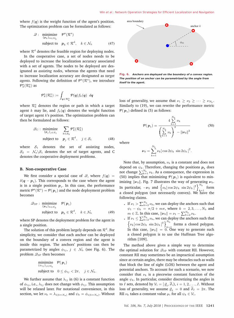
Win et al.: Network Operation Strategies for Efficient Localization and Navigation
where f(q) is the weight function of the agent’s position.
The optimization problem can be formulated as follows:
Q : minimize{pk}k∈Nb
Pa(Ra)
subject to pk ∈ Rd, k ∈ Nb (47)
where Rd denotes the feasible region for deploying nodes.
In the cooperative case, a set of nodes needs to be
deployed to increase the localization accuracy associated
with a set of agents. The nodes to be deployed are des-
ignated as assisting nodes, whereas the agents that need
to increase localization accuracy are designated as target
agents. Following the definition of Pa(Ra), we introduce
Pak(Ra
k) as
Pak(Ra
k) :=
(q∈Ra
k
P(q)fk(q) dq
where Rak denotes the region or path in which a target
agent k may lie, and fk(q) denotes the weight function
of target agent k’s position. The optimization problem can
then be formulated as follows:
QC : minimize{pj}j∈S1
�k∈S2
Pak(Ra
k)
subject to pj ∈ Rd, j ∈ S1 (48)
where S1 denotes the set of assisting nodes,
S2 = Na\S1 denotes the set of target agents, and C
denotes the cooperative deployment problems.
B. Non-cooperative Case
We first consider a special case of Q, where f(q) =
δ(q − p1). This corresponds to the case where the agent
is in a single position p1. In this case, the performance
metric Pa(Ra) = P( p1) and the node deployment problem
becomes
QSP : minimize{pk}k∈Nb
P( p1)
subject to pk ∈ Rd, k ∈ Nb (49)
where SP denotes the deployment problem for the agent in
a single position.
The solution of this problem largely depends on Rd. For
simplicity, we consider that each anchor can be deployed
on the boundary of a convex region and the agent is
inside this region. The anchors’ positions can then be
parametrized by angles φ1j , j ∈ Nb (see Fig. 6). The
problem QSP then becomes
minimize{φ1j}j∈Nb
P( p1)
subject to 0 ≤ φ1j < 2π, j ∈ Nb.
We further assume that λ1j in (6) is a constant function
of φ1j , i.e., λ1j does not change with φ1j . This assumption
will be relaxed later. For notational convenience, in this
section, we let νk = λ1(k+Na) and ψk = φ1(k+Na). Without
Fig. 6. Anchors are deployed on the boundary of a convex region.
The position of an anchor can be parametrized by the angle from
itself to the agent.
loss of generality, we assume that ν1 ≥ ν2 ≥ · · · ≥ νNb .
Similarly to (19), we can rewrite the performance metric
P( p1) defined in (5) as follows:
P(p1) =
4Nb k=1
νk�Nb k=1
νk
�2
− ‖ν0‖2
(50)
where
ν0 =
Nb�k=1
νk[ cos 2ψk sin 2ψk ]T.
Note that, by assumption, νk is a constant and does not
depend on ψk. Therefore, changing the positions pk does
not change Nb
k=1 νk. As a consequence, the expression in
(50) implies that minimizing P( p1) is equivalent to min-
imizing ‖ν0‖. Fig. 7 illustrates the way of generating ν0.
In particular, −ν0 and�
νk[ cos 2ψk sin 2ψk ]T�Nb
k=1form
a closed polygon (not necessarily convex). We have the
following claims.
� If ν1 > Nb
k=2 νk, we can deploy the anchors such that
ψ1 − ψk = π/2 + mπ, where k = 2, 3, . . . , Nb and
m ∈ Z. In this case, ‖ν0‖ = ν1 − Nbk=2 νk.
� If ν1 ≤ Nbk=2 νk, we can deploy the anchors such that�
νk[ cos 2ψk sin 2ψk ]T�Nb
k=1forms a closed polygon.
In this case, ‖ν0‖ = 0. One way to generate such
a closed polygon is to use the Huffman Tree algo-
rithm [109].
The method above gives a simple way to determine
the optimal solution for QSP with constant RII. However,
constant RII may sometimes be an impractical assumption
since at certain angles, there may be obstacles such as walls
that block the line of sight (LOS) between the agent and
potential anchors. To account for such a scenario, we now
consider that νk is a piecewise constant function of the
angle ψk. In particular, consider discretizing the angles in
to I sets, denoted by Vi = [ ϑi, ϑi), i = 1, 2, . . . , I . Without
loss of generality, we assume ϑ1 = 0 and ϑI = 2π. The
RII νk takes a constant value μi for all ψk ∈ Vi.
Vol. 106, No. 7, July 2018 | PROCEEDINGS OF THE IEEE 1241
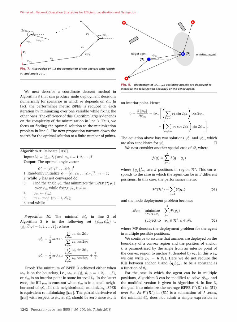
Win et al.: Network Operation Strategies for Efficient Localization and Navigation
Fig. 7. Illustration of ν0: the summation of the vectors with length
νk and angle 2ψk.
We next describe a coordinate descent method in
Algorithm 3 that can produce node deployment decisions
numerically for scenarios in which νk depends on ψk. In
fact, the performance metric iSPEB is reduced in each
iteration by minimizing over one variable while fixing the
other ones. The efficiency of this algorithm largely depends
on the complexity of the minimization in line 3. Thus, we
focus on finding the optimal solution to the minimization
problem in line 3. The next proposition narrows down the
search for the optimal solution to a finite number of points.
Algorithm 3: Relocate [108]
Input: Vi = [ ϑi, ϑi ) and μi, i = 1, 2, . . . , I
Output: The optimal angle vector
ψ∗ = [ψ∗1 ψ∗
2 . . . ψ∗Nb
]T
1: Randomly initialize ψ = [ψ1 ψ2 . . . ψNb ]T, m = 1;
2: while ψ has not converged do
3: Find the angle ψ∗m that minimizes the iSPEB P(p1)
over ψm while fixing ψk, k �= m;
4: ψm ← ψ∗m;
5: m ←mod (m + 1, Nb);
6: end while
Proposition 10: The minimal ψ∗m in line 3 of
Algorithm 3 is in the following set {ψ1m, ψ2
m} ∪{ϑi, ϑi, i = 1, 2, . . . , I}, where
ψ1m =
1
2arctan
k =m
νk sin 2ψk k =m
νk cos 2ψk
ψ2m =
1
2arctan
k =m
νk sin 2ψk k =m
νk cos 2ψk
+π
2.
Proof: The minimum of iSPEB is achieved either when
ψm is on the boundary, i.e., ψm ∈ {ϑi, ϑi, i = 1, 2, . . . , I},
or ψm is an interior point in some interval Vi. In the latter
case, the RII μm is constant when ψm is in a small neigh-
borhood of ψ∗m. In this neighborhood, minimizing iSPEB
is equivalent to minimizing ‖ν0‖. The partial derivative of
‖ν0‖ with respect to ψm at ψ∗m should be zero since ψm is
Fig. 8. Illustration of Q�−��: assisting agents are deployed to
increase the localization accuracy of the other agent.
an interior point. Hence
0 =∂ ‖ν0‖∂ψm
= 4νm
���k =m
νk sin 2ψk
�cos 2ψm
−��
k =m
νk cos 2ψk
�sin 2ψm
�.
The equation above has two solutions ψ1m and ψ2
m, which
are also candidates for ψ∗m. �
We next consider another special case of Q, where
f(q) =
J�j=1
δ(q − qj)
where {qj}Jj=1 are J positions in region Ra. This corre-
sponds to the case in which the agent can be in J different
positions. In this case, the performance metric
Pa(Ra) =
J�j=1
P(qj) (51)
and the node deployment problem becomes
QMP : minimize{pk}k∈Nb
J�j=1
P(qj)
subject to pk ∈ Rd, k ∈ Nb (52)
where MP denotes the deployment problem for the agent
in multiple possible positions.
We continue to assume that anchors are deployed on the
boundary of a convex region and the position of anchor
k is parametrized by the angle from an interior point of
the convex region to anchor k, denoted by θk. In this way,
we can write pk = h(θk). Here we do not require the
RIIs between anchor k and {qj}Jj=1 to be a constant as
a function of θk.
For the case in which the agent can be in multiple
positions, Algorithm 3 can be modified to solve QMP and
the modified version is given in Algorithm 4. In line 3,
the goal is to minimize the average iSPEB Pa(Ra) in (51)
over θm. As Pa(Ra) in (51) is a summation of J terms,
the minimal θ∗m does not admit a simple expression as
1242 PROCEEDINGS OF THE IEEE | Vol. 106, No. 7, July 2018
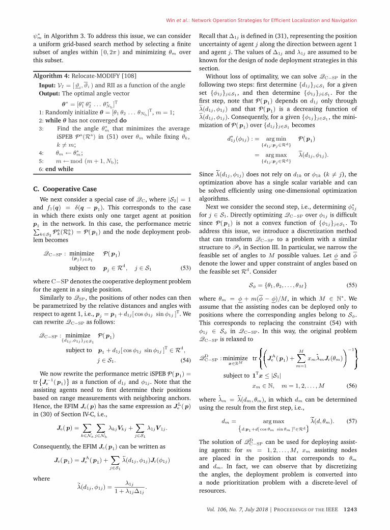
Win et al.: Network Operation Strategies for Efficient Localization and Navigation
ψ∗m in Algorithm 3. To address this issue, we can consider
a uniform grid-based search method by selecting a finite
subset of angles within [ 0, 2π ) and minimizing θm over
this subset.
Algorithm 4: Relocate-MODIFY [108]
Input: VI = [ ϑi, ϑi ) and RII as a function of the angle
Output: The optimal angle vector
θ∗ = [θ∗1 θ∗
2 . . . θ∗Nb
]T
1: Randomly initialize θ = [θ1 θ2 . . . θNb ]T, m = 1;
2: while θ has not converged do
3: Find the angle θ∗m that minimizes the average
iSPEB Pa(Ra) in (51) over θm while fixing θk,
k �= m;
4: θm ← θ∗m;
5: m ←mod (m + 1, Nb);
6: end while
C. Cooperative Case
We next consider a special case of QC, where |S2| = 1
and f1(q) = δ(q − p1). This corresponds to the case
in which there exists only one target agent at position
p1 in the network. In this case, the performance metric k∈S2
Pak(Ra
k) = P( p1) and the node deployment prob-
lem becomes
QC−SP : minimize{pj}j∈S1
P( p1)
subject to pj ∈ Rd, j ∈ S1 (53)
where C−SP denotes the cooperative deployment problem
for the agent in a single position.
Similarly to QSP, the positions of other nodes can then
be parametrized by the relative distances and angles with
respect to agent 1, i.e., pj = p1 +d1j [ cos φ1j sin φ1j ]T. We
can rewrite QC−SP as follows:
QC−SP : minimize{d1j ,φ1j}j∈S1
P(p1)
subject to p1 + d1j [ cos φ1j sin φ1j ]T ∈ Rd,
j ∈ S1. (54)
We now rewrite the performance metric iSPEB P(p1) =
tr�J−1
e (p1)�
as a function of d1j and φ1j . Note that the
assisting agents need to first determine their positions
based on range measurements with neighboring anchors.
Hence, the EFIM Je( p) has the same expression as JLe ( p)
in (30) of Section IV-C, i.e.,
Je( p) =�
k∈Na
�j∈Nb
λkjVkj +�j∈S1
λ1jV 1j .
Consequently, the EFIM Je(p1) can be written as
Je( p1) = JAe (p1) +
�j∈S1
�λ(d1j , φ1j)Jr(φ1j)
where �λ(d1j , φ1j) =λ1j
1 + λ1j∆1j
.
Recall that ∆1j is defined in (31), representing the position
uncertainty of agent j along the direction between agent 1
and agent j. The values of ∆1j and λ1j are assumed to be
known for the design of node deployment strategies in this
section.
Without loss of optimality, we can solve QC−SP in the
following two steps: first determine {d1j}j∈S1 for a given
set {φ1j}j∈S1 , and then determine {φ1j}j∈S1 . For the
first step, note that P( p1) depends on d1j only through�λ(d1j , φ1j) and that P(p1) is a decreasing function of�λ(d1j , φ1j). Consequently, for a given {φ1j}j∈S1 , the mini-
mization of P( p1) over {d1j}j∈S1 becomes
d∗1j(φ1j) : = arg min
{d1j :pj∈Rd}
P(p1)
= arg max{d1j :pj∈Rd}
�λ(d1j , φ1j).
Since �λ(d1j , φ1j) does not rely on d1k or φ1k (k �= j), the
optimization above has a single scalar variable and can
be solved efficiently using one-dimensional optimization
algorithms.
Next we consider the second step, i.e., determining φ∗1j
for j ∈ S1. Directly optimizing QC−SP over φ1j is difficult
since P(p1) is not a convex function of {φ1j}j∈S1 . To
address this issue, we introduce a discretization method
that can transform QC−SP to a problem with a similar
structure to Pk in Section III. In particular, we narrow the
feasible set of angles to M possible values. Let φ and φ
denote the lower and upper constraint of angles based on
the feasible set Rd. Consider
Sφ = {θ1, θ2, . . . , θM} (55)
where θm = φ + m(φ − φ)/M , in which M ∈ N∗. We
assume that the assisting nodes can be deployed only to
positions where the corresponding angles belong to Sφ.
This corresponds to replacing the constraint (54) with
φ1j ∈ Sφ in QC−SP. In this way, the original problem
QC−SP is relaxed to
QDC−SP : minimize
x∈RMtr
����
JAe (p1) +
M�m=1
xm�λmJr(θm)
�−1)*+
subject to 1Tx ≤ |S1|
xm ∈ N, m = 1, 2, . . . , M (56)
where �λm = �λ(dm, θm), in which dm can be determined
using the result from the first step, i.e.,
dm = arg max�d:p1+d[ cos θm sin θm ]T∈Rd
��λ(d, θm). (57)
The solution of QDC−SP can be used for deploying assist-
ing agents: for m = 1, 2, . . . , M , xm assisting nodes
are placed in the position that corresponds to θm
and dm. In fact, we can observe that by discretizing
the angles, the deployment problem is converted into
a node prioritization problem with a discrete-level of
resources.
Vol. 106, No. 7, July 2018 | PROCEEDINGS OF THE IEEE 1243
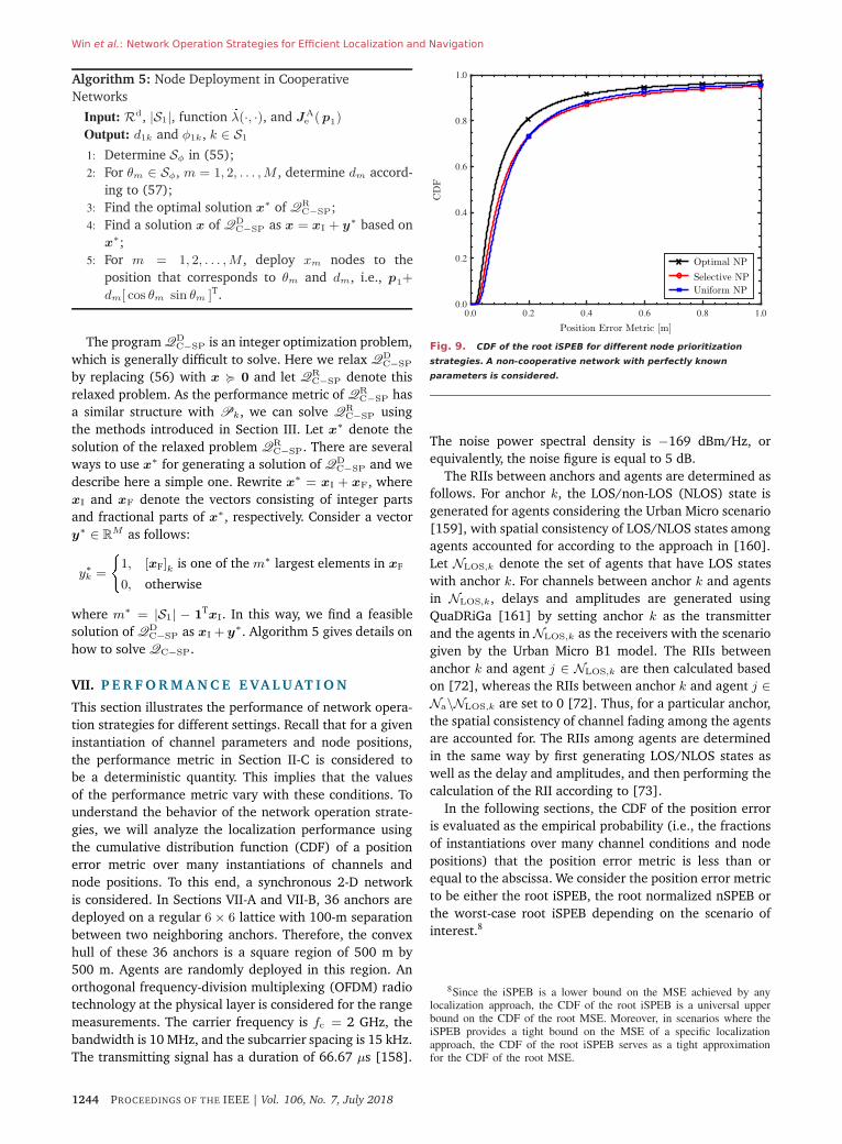
Win et al.: Network Operation Strategies for Efficient Localization and Navigation
Algorithm 5: Node Deployment in Cooperative
Networks
Input: Rd, |S1|, function �λ(·, ·), and JAe ( p1)
Output: d1k and φ1k, k ∈ S1
1: Determine Sφ in (55);
2: For θm ∈ Sφ, m = 1, 2, . . . , M , determine dm accord-
ing to (57);
3: Find the optimal solution x∗ of QRC−SP;
4: Find a solution x of QDC−SP as x = xI + y∗ based on
x∗;
5: For m = 1, 2, . . . , M , deploy xm nodes to the
position that corresponds to θm and dm, i.e., p1+
dm[ cos θm sin θm ]T.
The program QDC−SP is an integer optimization problem,
which is generally difficult to solve. Here we relax QDC−SP
by replacing (56) with x � 0 and let QRC−SP denote this
relaxed problem. As the performance metric of QRC−SP has
a similar structure with Pk, we can solve QRC−SP using
the methods introduced in Section III. Let x∗ denote the
solution of the relaxed problem QRC−SP. There are several
ways to use x∗ for generating a solution of QDC−SP and we
describe here a simple one. Rewrite x∗ = xI + xF, where
xI and xF denote the vectors consisting of integer parts
and fractional parts of x∗, respectively. Consider a vector
y∗ ∈ RM as follows:
y∗k =
�1, [xF]k is one of the m∗ largest elements in xF
0, otherwise
where m∗ = |S1| − 1TxI. In this way, we find a feasible
solution of QDC−SP as xI + y∗. Algorithm 5 gives details on
how to solve QC−SP.
VII. P E R F O R M A N C E E VA L U AT I O N
This section illustrates the performance of network opera-
tion strategies for different settings. Recall that for a given
instantiation of channel parameters and node positions,
the performance metric in Section II-C is considered to
be a deterministic quantity. This implies that the values
of the performance metric vary with these conditions. To
understand the behavior of the network operation strate-
gies, we will analyze the localization performance using
the cumulative distribution function (CDF) of a position
error metric over many instantiations of channels and
node positions. To this end, a synchronous 2-D network
is considered. In Sections VII-A and VII-B, 36 anchors are
deployed on a regular 6 × 6 lattice with 100-m separation
between two neighboring anchors. Therefore, the convex
hull of these 36 anchors is a square region of 500 m by
500 m. Agents are randomly deployed in this region. An
orthogonal frequency-division multiplexing (OFDM) radio
technology at the physical layer is considered for the range
measurements. The carrier frequency is fc = 2 GHz, the
bandwidth is 10 MHz, and the subcarrier spacing is 15 kHz.
The transmitting signal has a duration of 66.67 μs [158].
Fig. 9. CDF of the root iSPEB for different node prioritization
strategies. A non-cooperative network with perfectly known
parameters is considered.
The noise power spectral density is −169 dBm/Hz, or
equivalently, the noise figure is equal to 5 dB.
The RIIs between anchors and agents are determined as
follows. For anchor k, the LOS/non-LOS (NLOS) state is
generated for agents considering the Urban Micro scenario
[159], with spatial consistency of LOS/NLOS states among
agents accounted for according to the approach in [160].
Let NLOS,k denote the set of agents that have LOS states
with anchor k. For channels between anchor k and agents
in NLOS,k, delays and amplitudes are generated using
QuaDRiGa [161] by setting anchor k as the transmitter
and the agents in NLOS,k as the receivers with the scenario
given by the Urban Micro B1 model. The RIIs between
anchor k and agent j ∈ NLOS,k are then calculated based
on [72], whereas the RIIs between anchor k and agent j ∈Na\NLOS,k are set to 0 [72]. Thus, for a particular anchor,
the spatial consistency of channel fading among the agents
are accounted for. The RIIs among agents are determined
in the same way by first generating LOS/NLOS states as
well as the delay and amplitudes, and then performing the
calculation of the RII according to [73].
In the following sections, the CDF of the position error
is evaluated as the empirical probability (i.e., the fractions
of instantiations over many channel conditions and node
positions) that the position error metric is less than or
equal to the abscissa. We consider the position error metric
to be either the root iSPEB, the root normalized nSPEB or
the worst-case root iSPEB depending on the scenario of
interest.8
8Since the iSPEB is a lower bound on the MSE achieved by anylocalization approach, the CDF of the root iSPEB is a universal upperbound on the CDF of the root MSE. Moreover, in scenarios where theiSPEB provides a tight bound on the MSE of a specific localizationapproach, the CDF of the root iSPEB serves as a tight approximationfor the CDF of the root MSE.
1244 PROCEEDINGS OF THE IEEE | Vol. 106, No. 7, July 2018
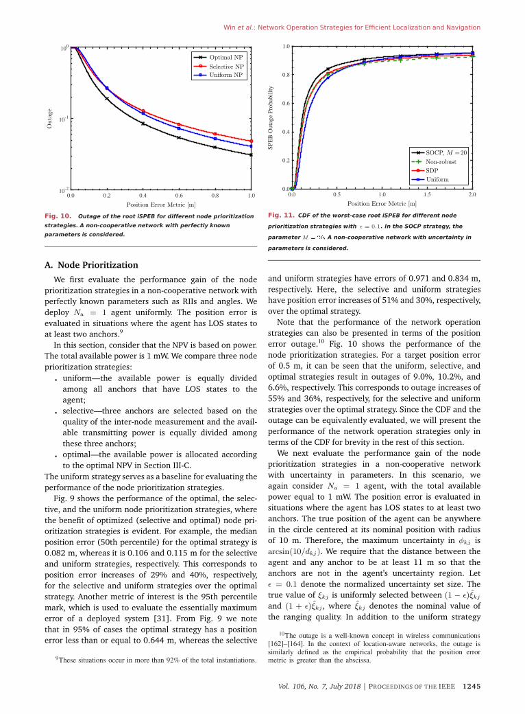
Win et al.: Network Operation Strategies for Efficient Localization and Navigation
Fig. 10. Outage of the root iSPEB for different node prioritization
strategies. A non-cooperative network with perfectly known
parameters is considered.
A. Node Prioritization
We first evaluate the performance gain of the node
prioritization strategies in a non-cooperative network with
perfectly known parameters such as RIIs and angles. We
deploy Na = 1 agent uniformly. The position error is
evaluated in situations where the agent has LOS states to
at least two anchors.9
In this section, consider that the NPV is based on power.
The total available power is 1 mW. We compare three node
prioritization strategies:
� uniform—the available power is equally divided
among all anchors that have LOS states to the
agent;
� selective—three anchors are selected based on the
quality of the inter-node measurement and the avail-
able transmitting power is equally divided among
these three anchors;
� optimal—the available power is allocated according
to the optimal NPV in Section III-C.
The uniform strategy serves as a baseline for evaluating the
performance of the node prioritization strategies.
Fig. 9 shows the performance of the optimal, the selec-
tive, and the uniform node prioritization strategies, where
the benefit of optimized (selective and optimal) node pri-
oritization strategies is evident. For example, the median
position error (50th percentile) for the optimal strategy is
0.082 m, whereas it is 0.106 and 0.115 m for the selective
and uniform strategies, respectively. This corresponds to
position error increases of 29% and 40%, respectively,
for the selective and uniform strategies over the optimal
strategy. Another metric of interest is the 95th percentile
mark, which is used to evaluate the essentially maximum
error of a deployed system [31]. From Fig. 9 we note
that in 95% of cases the optimal strategy has a position
error less than or equal to 0.644 m, whereas the selective
9These situations occur in more than 92% of the total instantiations.
Fig. 11. CDF of the worst-case root iSPEB for different node
prioritization strategies with ǫ = 0.1. In the SOCP strategy, the
parameter M � ��. A non-cooperative network with uncertainty in
parameters is considered.
and uniform strategies have errors of 0.971 and 0.834 m,
respectively. Here, the selective and uniform strategies
have position error increases of 51% and 30%, respectively,
over the optimal strategy.
Note that the performance of the network operation
strategies can also be presented in terms of the position
error outage.10 Fig. 10 shows the performance of the
node prioritization strategies. For a target position error
of 0.5 m, it can be seen that the uniform, selective, and
optimal strategies result in outages of 9.0%, 10.2%, and
6.6%, respectively. This corresponds to outage increases of
55% and 36%, respectively, for the selective and uniform
strategies over the optimal strategy. Since the CDF and the
outage can be equivalently evaluated, we will present the
performance of the network operation strategies only in
terms of the CDF for brevity in the rest of this section.
We next evaluate the performance gain of the node
prioritization strategies in a non-cooperative network
with uncertainty in parameters. In this scenario, we
again consider Na = 1 agent, with the total available
power equal to 1 mW. The position error is evaluated in
situations where the agent has LOS states to at least two
anchors. The true position of the agent can be anywhere
in the circle centered at its nominal position with radius
of 10 m. Therefore, the maximum uncertainty in φkj is
arcsin(10/dkj). We require that the distance between the
agent and any anchor to be at least 11 m so that the
anchors are not in the agent’s uncertainty region. Let
ǫ = 0.1 denote the normalized uncertainty set size. The
true value of ξkj is uniformly selected between (1 − ǫ)ξkj
and (1 + ǫ)ξkj , where ξkj denotes the nominal value of
the ranging quality. In addition to the uniform strategy
10The outage is a well-known concept in wireless communications[162]–[164]. In the context of location-aware networks, the outage issimilarly defined as the empirical probability that the position errormetric is greater than the abscissa.
Vol. 106, No. 7, July 2018 | PROCEEDINGS OF THE IEEE 1245
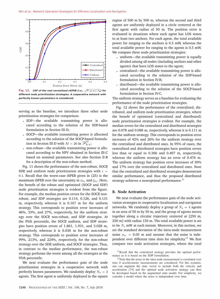
Win et al.: Network Operation Strategies for Efficient Localization and Navigation
Fig. 12. CDF of the root normalized nSPEB (i.e.,�P� p�x�/N�) for
different node prioritization strategies. A cooperative network with
perfectly known parameters is considered.
serving as the baseline, we introduce three other node
prioritization strategies for comparison:
� SDP—the available transmitting power is allo-
cated according to the solution of the SDP-based
formulation in Section III-D;
� SOCP—the available transmitting power is allocated
according to the solution of the SOCP-based formula-
tion in Section III-D with M = 20 in PM
R,k;
� non-robust—the available transmitting power is allo-
cated according to the NPV obtained in Section III-C
based on nominal parameters. See also Section II-B
for a description of the non-robust method.
Fig. 11 shows the performance of the non-robust, SOCP,
SDP, and uniform node prioritization strategies with ǫ =
0.1. Recall that the worst-case iSPEB given in (25) is the
maximum iSPEB over the uncertainty in φkj and ξkj . Here,
the benefit of the robust and optimized (SOCP and SDP)
node prioritization strategies is evident from the figure.
For example, the median position errors for the SOCP, non-
robust, and SDP strategies are 0.114, 0.126, and 0.131
m, respectively, whereas it is 0.167 m for the uniform
strategy. This corresponds to position error increases of
46%, 33%, and 27%, respectively, for the uniform strat-
egy over the SOCP, non-robust, and SDP strategies. At
the 95th percentile, the SOCP, uniform, and SDP strate-
gies have position errors of 1.861, 1.931, and 3.028 m,
respectively, whereas it is 6.036 m for the non-robust
strategy. This corresponds to position error increases of
99%, 213%, and 224%, respectively, for the non-robust
strategy over the SDP, uniform, and SOCP strategies. Thus,
in contrast to the median performance, the non-robust
strategy performs the worst among all the strategies at the
95th percentile.
We next evaluate the performance gain of the node
prioritization strategies in a cooperative network with
perfectly known parameters. We randomly deploy Na = 3
agents. The first agent is uniformly deployed in the square
region of 500 m by 500 m, whereas the second and third
agents are uniformly deployed in a circle centered at the
first agent with radius of 50 m. The position error is
evaluated in situations where each agent has LOS states
to at least two anchors. For each agent, the total available
power for ranging to the anchors is 0.5 mW, whereas the
total available power for ranging to the agents is 0.5 mW.
We compare three node prioritization strategies:
� uniform—the available transmitting power is equally
divided among all nodes (including anchors and other
agents) that have LOS states to the agent;
� centralized—the available transmitting power is allo-
cated according to the solution of the SDP-based
formulation in Section IV-B;
� distributed—the available transmitting power is allo-
cated according to the solution of the SOCP-based
formulation in Section IV-C.
The uniform strategy serves as a baseline for evaluating the
performance of the node prioritization strategies.
Fig. 12 shows the performance of the centralized, dis-
tributed, and uniform node prioritization strategies, where
the benefit of optimized (centralized and distributed)
node prioritization strategies is evident. For example, the
median errors for the centralized and distributed strategies
are 0.078 and 0.088 m, respectively, whereas it is 0.111 m
for the uniform strategy. This corresponds to position error
increases of 42% and 26% for the uniform strategy over
the centralized and distributed ones. In 95% of cases, the
centralized and distributed strategies have position errors
less than or equal to 0.366 and 0.407 m, respectively,
whereas the uniform strategy has an error of 0.476 m.
The uniform strategy has position error increases of 30%
and 17% over the centralized and distributed ones. Note
that the centralized and distributed strategies demonstrate
similar performance, and thus the proposed distributed
strategy achieves a nearoptimal performance.11
B. Node Activation
We next evaluate the performance gain of the node acti-
vation strategies in cooperative localization and navigation
networks. We randomly deploy a group of Na = 4 agents
in an area of 50 m by 50 m, and the group of agents moves
together along a circular trajectory centered at [250 m,
250 m] with radius 150 m. The total available power is set
to be Na mW at each instant. Moreover, in this section, we
set the standard deviation of the intra-node measurement
noise σm = 0.05 m and assume that the noise is inde-
pendent over different time slots for simplicity.12 We first
compare two node activation strategies, where the total
11Recall that the centralized strategy provides the optimal perfor-mance as it is based on the SDP formulation.
12Note that the noise in the intra-node measurement is correlated overtime if accelerometer measurements are considered. For this scenario,one can augment the state vector to include both the velocity andacceleration [74] and the optimal node activation strategy can thenbe developed based on the augmented state model. For simplicity, weconsider a model where the noise is independent over time.
1246 PROCEEDINGS OF THE IEEE | Vol. 106, No. 7, July 2018
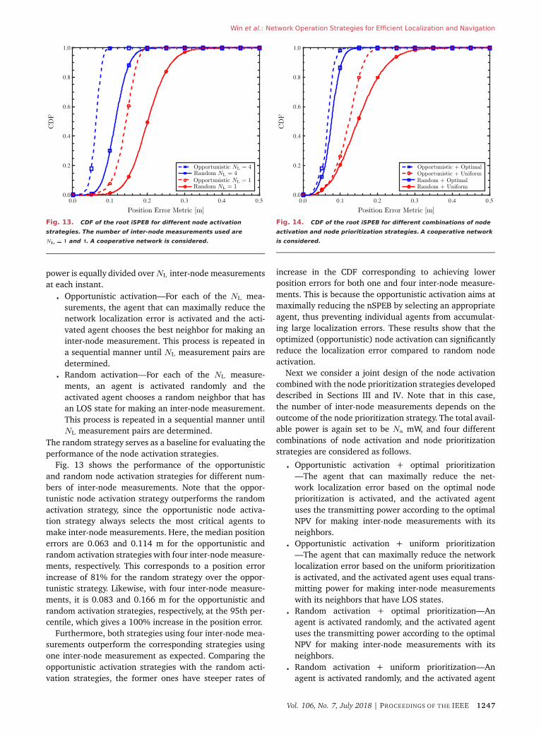
Win et al.: Network Operation Strategies for Efficient Localization and Navigation
Fig. 13. CDF of the root iSPEB for different node activation
strategies. The number of inter-node measurements used are
N� � � and �. A cooperative network is considered.
power is equally divided over NL inter-node measurements
at each instant.
� Opportunistic activation—For each of the NL mea-
surements, the agent that can maximally reduce the
network localization error is activated and the acti-
vated agent chooses the best neighbor for making an
inter-node measurement. This process is repeated in
a sequential manner until NL measurement pairs are
determined.
� Random activation—For each of the NL measure-
ments, an agent is activated randomly and the
activated agent chooses a random neighbor that has
an LOS state for making an inter-node measurement.
This process is repeated in a sequential manner until
NL measurement pairs are determined.
The random strategy serves as a baseline for evaluating the
performance of the node activation strategies.
Fig. 13 shows the performance of the opportunistic
and random node activation strategies for different num-
bers of inter-node measurements. Note that the oppor-
tunistic node activation strategy outperforms the random
activation strategy, since the opportunistic node activa-
tion strategy always selects the most critical agents to
make inter-node measurements. Here, the median position
errors are 0.063 and 0.114 m for the opportunistic and
random activation strategies with four inter-node measure-
ments, respectively. This corresponds to a position error
increase of 81% for the random strategy over the oppor-
tunistic strategy. Likewise, with four inter-node measure-
ments, it is 0.083 and 0.166 m for the opportunistic and
random activation strategies, respectively, at the 95th per-
centile, which gives a 100% increase in the position error.
Furthermore, both strategies using four inter-node mea-
surements outperform the corresponding strategies using
one inter-node measurement as expected. Comparing the
opportunistic activation strategies with the random acti-
vation strategies, the former ones have steeper rates of
Fig. 14. CDF of the root iSPEB for different combinations of node
activation and node prioritization strategies. A cooperative network
is considered.
increase in the CDF corresponding to achieving lower
position errors for both one and four inter-node measure-
ments. This is because the opportunistic activation aims at
maximally reducing the nSPEB by selecting an appropriate
agent, thus preventing individual agents from accumulat-
ing large localization errors. These results show that the
optimized (opportunistic) node activation can significantly
reduce the localization error compared to random node
activation.
Next we consider a joint design of the node activation
combined with the node prioritization strategies developed
described in Sections III and IV. Note that in this case,
the number of inter-node measurements depends on the
outcome of the node prioritization strategy. The total avail-
able power is again set to be Na mW, and four different
combinations of node activation and node prioritization
strategies are considered as follows.
� Opportunistic activation + optimal prioritization
—The agent that can maximally reduce the net-
work localization error based on the optimal node
prioritization is activated, and the activated agent
uses the transmitting power according to the optimal
NPV for making inter-node measurements with its
neighbors.
� Opportunistic activation + uniform prioritization
—The agent that can maximally reduce the network
localization error based on the uniform prioritization
is activated, and the activated agent uses equal trans-
mitting power for making inter-node measurements
with its neighbors that have LOS states.
� Random activation + optimal prioritization—An
agent is activated randomly, and the activated agent
uses the transmitting power according to the optimal
NPV for making inter-node measurements with its
neighbors.
� Random activation + uniform prioritization—An
agent is activated randomly, and the activated agent
Vol. 106, No. 7, July 2018 | PROCEEDINGS OF THE IEEE 1247
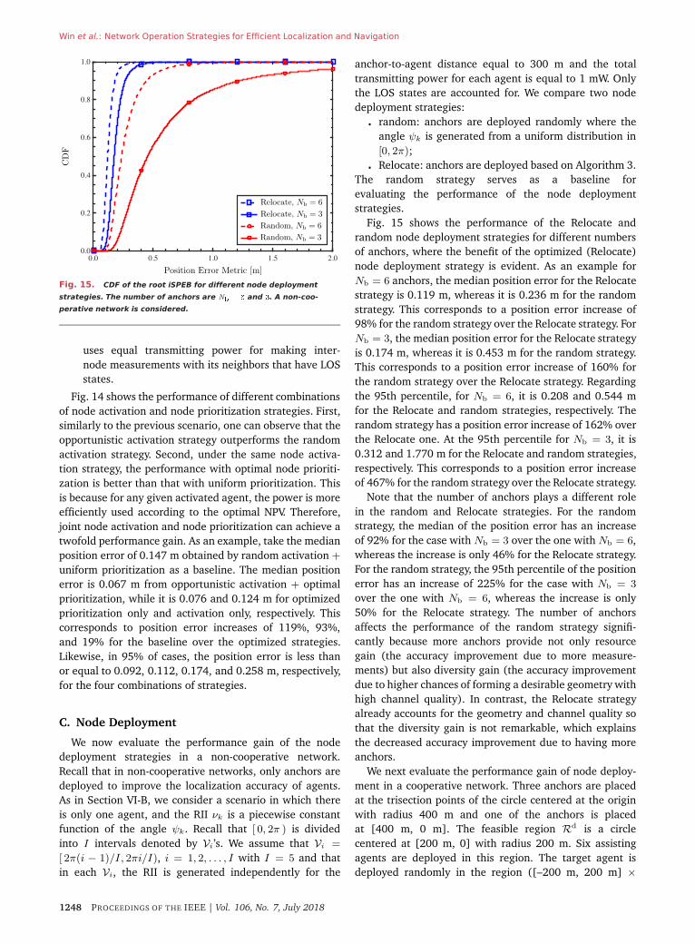
Win et al.: Network Operation Strategies for Efficient Localization and Navigation
Fig. 15. CDF of the root iSPEB for different node deployment
strategies. The number of anchors are N� � and . A non-coo-
perative network is considered.
uses equal transmitting power for making inter-
node measurements with its neighbors that have LOS
states.
Fig. 14 shows the performance of different combinations
of node activation and node prioritization strategies. First,
similarly to the previous scenario, one can observe that the
opportunistic activation strategy outperforms the random
activation strategy. Second, under the same node activa-
tion strategy, the performance with optimal node prioriti-
zation is better than that with uniform prioritization. This
is because for any given activated agent, the power is more
efficiently used according to the optimal NPV. Therefore,
joint node activation and node prioritization can achieve a
twofold performance gain. As an example, take the median
position error of 0.147 m obtained by random activation +
uniform prioritization as a baseline. The median position
error is 0.067 m from opportunistic activation + optimal
prioritization, while it is 0.076 and 0.124 m for optimized
prioritization only and activation only, respectively. This
corresponds to position error increases of 119%, 93%,
and 19% for the baseline over the optimized strategies.
Likewise, in 95% of cases, the position error is less than
or equal to 0.092, 0.112, 0.174, and 0.258 m, respectively,
for the four combinations of strategies.
C. Node Deployment
We now evaluate the performance gain of the node
deployment strategies in a non-cooperative network.
Recall that in non-cooperative networks, only anchors are
deployed to improve the localization accuracy of agents.
As in Section VI-B, we consider a scenario in which there
is only one agent, and the RII νk is a piecewise constant
function of the angle ψk. Recall that [ 0, 2π ) is divided
into I intervals denoted by Vi ’s. We assume that Vi =
[ 2π(i − 1)/I, 2πi/I), i = 1, 2, . . . , I with I = 5 and that
in each Vi, the RII is generated independently for the
anchor-to-agent distance equal to 300 m and the total
transmitting power for each agent is equal to 1 mW. Only
the LOS states are accounted for. We compare two node
deployment strategies:
� random: anchors are deployed randomly where the
angle ψk is generated from a uniform distribution in
[0, 2π);
� Relocate: anchors are deployed based on Algorithm 3.
The random strategy serves as a baseline for
evaluating the performance of the node deployment
strategies.
Fig. 15 shows the performance of the Relocate and
random node deployment strategies for different numbers
of anchors, where the benefit of the optimized (Relocate)
node deployment strategy is evident. As an example for
Nb = 6 anchors, the median position error for the Relocate
strategy is 0.119 m, whereas it is 0.236 m for the random
strategy. This corresponds to a position error increase of
98% for the random strategy over the Relocate strategy. For
Nb = 3, the median position error for the Relocate strategy
is 0.174 m, whereas it is 0.453 m for the random strategy.
This corresponds to a position error increase of 160% for
the random strategy over the Relocate strategy. Regarding
the 95th percentile, for Nb = 6, it is 0.208 and 0.544 m
for the Relocate and random strategies, respectively. The
random strategy has a position error increase of 162% over
the Relocate one. At the 95th percentile for Nb = 3, it is
0.312 and 1.770 m for the Relocate and random strategies,
respectively. This corresponds to a position error increase
of 467% for the random strategy over the Relocate strategy.
Note that the number of anchors plays a different role
in the random and Relocate strategies. For the random
strategy, the median of the position error has an increase
of 92% for the case with Nb = 3 over the one with Nb = 6,
whereas the increase is only 46% for the Relocate strategy.
For the random strategy, the 95th percentile of the position
error has an increase of 225% for the case with Nb = 3
over the one with Nb = 6, whereas the increase is only
50% for the Relocate strategy. The number of anchors
affects the performance of the random strategy signifi-
cantly because more anchors provide not only resource
gain (the accuracy improvement due to more measure-
ments) but also diversity gain (the accuracy improvement
due to higher chances of forming a desirable geometry with
high channel quality). In contrast, the Relocate strategy
already accounts for the geometry and channel quality so
that the diversity gain is not remarkable, which explains
the decreased accuracy improvement due to having more
anchors.
We next evaluate the performance gain of node deploy-
ment in a cooperative network. Three anchors are placed
at the trisection points of the circle centered at the origin
with radius 400 m and one of the anchors is placed
at [400 m, 0 m]. The feasible region Rd is a circle
centered at [200 m, 0] with radius 200 m. Six assisting
agents are deployed in this region. The target agent is
deployed randomly in the region ([–200 m, 200 m] ×
1248 PROCEEDINGS OF THE IEEE | Vol. 106, No. 7, July 2018
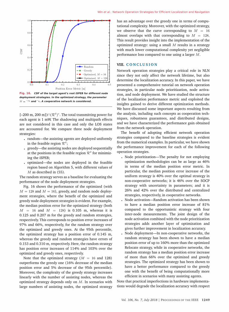
Win et al.: Network Operation Strategies for Efficient Localization and Navigation
Fig. 16. CDF of the target agent’s root iSPEB for different node
deployment strategies. In the optimized strategy, the parameter
M � ��� and �. A cooperative network is considered.
[–200 m, 200 m])∩(Rd)c. The total transmitting power for
each agent is 1 mW. The shadowing and multipath effects
are not considered in this case and only the LOS states
are accounted for. We compare three node deployment
strategies:
� random—the assisting agents are deployed uniformly
in the feasible region Rd;
� greedy—the assisting nodes are deployed sequentially
at the positions in the feasible region Rd for minimiz-
ing the iSPEB;
� optimized—the nodes are deployed in the feasible
region based on Algorithm 5, with different values of
M as described in (55).
The random strategy serves as a baseline for evaluating the
performance of the node deployment strategies.
Fig. 16 shows the performance of the optimized (with
M = 128 and M = 16), greedy, and random node deploy-
ment strategies, where the benefit of the optimized and
greedy node deployment strategies is evident. For example,
the median position error for the optimized strategy (both
M = 16 and M = 128) is 0.105 m, whereas it is
0.125 and 0.207 m for the greedy and random strategies,
respectively. This corresponds to position error increases of
97% and 66%, respectively, for the random strategy over
the optimized and greedy ones. At the 95th percentile,
the optimized strategy has a position error of 0.145 m,
whereas the greedy and random strategies have errors of
0.153 and 0.310 m, respectively. Here, the random strategy
has position error increases of 114% and 103% over the
optimized and greedy ones, respectively.
Note that the optimized strategy (M = 16 and 128)
outperforms the greedy one (16% decrease of the median
position error and 5% decrease of the 95th percentile).
Moreover, the complexity of the greedy strategy increases
linearly with the number of assisting nodes, whereas the
optimized strategy depends only on M . In scenarios with
large numbers of assisting nodes, the optimized strategy
has an advantage over the greedy one in terms of compu-
tational complexity. Moreover, with the optimized strategy,
we observe that the curve corresponding to M = 16
almost overlaps with that corresponding to M = 128.
This result provides insight into the implementation of the
optimized strategy: using a small M results in a strategy
with much lower computational complexity yet negligible
performance loss compared to one using a larger M .
VIII. C O N C L U S I O N
Network operation strategies play a critical role in NLN
since they not only affect the network lifetime, but also
determine the localization accuracy. In this paper, we have
presented a comprehensive tutorial on network operation
strategies, in particular node prioritization, node activa-
tion, and node deployment. We have studied the structure
of the localization performance metric and exploited the
insights gained to derive different optimization methods.
We have discussed some important aspects resulting from
the analysis, including such concepts as cooperation tech-
niques, robustness guarantees, and distributed designs,
and we have characterized the performance gain obtained
from the network operation.
The benefit of adopting efficient network operation
strategies compared to the baseline strategies is evident
from the numerical examples. In particular, we have shown
the performance improvement for each of the following
operation strategies.
� Node prioritization—The penalty for not employing
optimization methodologies can be as large as 46%
in terms of the median position error metric. In
particular, the median position error increase of the
uniform strategy is 40% over the optimal strategy in
non-cooperative networks; it is 46% over the SOCP
strategy with uncertainty in parameters; and it is
26% and 42% over the distributed and centralized
strategies, respectively, in cooperative networks.
� Node activation—Random activation has been shown
to have a median position error increase of 81%
compared to the opportunistic strategy with four
inter-node measurements. The joint design of the
node activation combined with the node prioritization
strategies adds another layer of optimization and
gives further improvement in localization accuracy.
� Node deployment—In non-cooperative networks, the
random strategy has been shown to have a median
position error of up to 160% more than the optimized
Relocate strategy, while in cooperative networks, the
random strategy has a median position error increase
of more than 66% over the optimized and greedy
strategies. The optimized strategy has been shown to
have a better performance compared to the greedy
one with the benefit of being computationally more
efficient in scenarios with many assisting agents.
Note that practical imperfections in hardware implementa-
tions would degrade the localization accuracy with respect
Vol. 106, No. 7, July 2018 | PROCEEDINGS OF THE IEEE 1249

Win et al.: Network Operation Strategies for Efficient Localization and Navigation
to that presented in this paper. However, the degradation
due to these imperfections would be similar for all the net-
work operation strategies presented, and thus the relative
accuracy improvement reported in this paper is expected to
still hold. While the performance characterization of vari-
ous NLN strategies has been exhaustively presented, there
are still open challenges to be addressed. For example,
the latency of position information is critical, especially in
highly dynamic environments. However, fewer analytical
methodologies have emerged to evaluate and optimize the
latency in localization and navigation networks. Moreover,
location secrecy and privacy are gradually becoming more
of a concern for location-based services, but techniques
that achieve both high accuracy and high secrecy in
NLN through network operation strategies are yet to be
developed. �
A c k n o w l e d g m e n t s
The authors would like to thank J. Chen, A. Conti, Z. Liu,
and S. Mazuelas for their helpful suggestions and careful
reading of the manuscript.
R E F E R E N C E S
[1] M. Z. Win et al., “Network localization and
navigation via cooperation,” IEEE Commun. Mag.,
vol. 49, no. 5, pp. 56–62,
May 2011.
[2] N. Bulusu, J. Heidemann, and D. Estrin, “GPS-less
low-cost outdoor localization for very small
devices,” IEEE Pers. Commun., vol. 7, no. 5, pp.
28–34, Oct. 2000.
[3] E. Paolini, A. Giorgetti, M. Chiani, R. Minutolo,
and M. Montanari, “Localization capability of
cooperative anti-intruder radar systems,” EURASIP
J. Adv. Signal Process., vol. 2008, Apr. 2008, Art.
no. 726854.
[4] S. Gezici et al., “Localization via ultra-wideband
radios: A look at positioning aspects for future
sensor networks,” IEEE Signal Process. Mag., vol.
22, no. 4, pp. 70–84, Jul. 2005.
[5] B. T. Robinson, “Who goes there?” IEEE Spectrum,
vol. 40, no. 10, pp. 42–47, Oct. 2003.
[6] F. Meyer et al., “Message passing algorithms for
scalable multitarget tracking,” Proc. IEEE, vol.
106, no. 2, pp. 221–259,
Feb. 2018.
[7] J. Guivant, E. Nebot, and S. Baiker, “Autonomous
navigation and map building using laser range
sensors in outdoor applications,” J. Robot. Syst.,
vol. 17, no. 10, pp. 565–583, Oct. 2000.
[8] S.-H. Lee and C. C. Chung, “Robust multirate
on-road vehicle localization for autonomous
highway driving vehicles,” IEEE Trans. Control
Syst. Technol., vol. 25, no. 2, pp. 577–589, Mar.
2017.
[9] G. Bresson, Z. Alsayed, L. Yu, and S. Glaser,
“Simultaneous localization and mapping: A survey
of current trends in autonomous driving,” IEEE
Trans. Intell. Veh., vol. 2, no. 3, pp. 194–220,
Sep. 2017.
[10] K. Witrisal et al., “High-accuracy localization for
assisted living: 5G systems will turn multipath
channels from foe to friend,” IEEE Signal Process.
Mag., vol. 33, no. 2, pp. 59–70, Mar. 2016.
[11] F. Buccafurri, G. Lax, S. Nicolazzo, and A. Nocera,
“Robust multirate on-road vehicle localization for
autonomous highway driving vehicles,” IEEE
Trans. Serv. Comput., to be published.
[12] P. Barsocchi, S. Chessa, F. Furfari, and F. Potortì,
“Evaluating ambient assisted living solutions: The
localization competition,” IEEE Pervas. Comput.,
vol. 12, no. 4, pp. 72–79, Oct. 2013.
[13] D. Miorandi, S. Sicari, F. De Pellegrini, and
I. Chlamtac, “Internet of Things: Vision,
applications and research challenges,” Ad Hoc
Netw., vol. 10, no. 7, pp. 1497–1516, Sep. 2012.
[14] S. D’Oro, L. Galluccio, G. Morabito, and
S. Palazzo, “Exploiting object group localization in
the Internet of Things: Performance analysis,”
IEEE Trans. Veh. Technol., vol. 64, no. 8, pp.
3645–3656, Aug. 2015.
[15] D. Zhang, L. T. Yang, M. Chen, S. Zhao, M. Guo,
and Y. Zhang, “Real-time locating systems using
active RFID for Internet of Things,” IEEE Syst. J.,
vol. 10, no. 3, pp. 1226–1235, Sep. 2016.
[16] F. Meyer, B. Etzlinger, Z. Liu, F. Hlawatsch, and
M. Z. Win, “Scalable cooperative synchronization
and navigation for the Internet of Things,” IEEE
Internet Things J., vol. 5, 2018, to appear.
[17] R. K. Ganti, F. Ye, and H. Lei, “Mobile
crowdsensing: Current state and future
challenges,” IEEE Commun. Mag., vol. 49, no. 11,
pp. 32–39, Nov. 2011.
[18] G. Cardone et al., “Fostering participation in smart
cities: A geo-social crowdsensing platform,” IEEE
Commun. Mag., vol. 51, no. 6, pp. 112–119, Jun.
2013.
[19] F. Zabini and A. Conti, “Inhomogeneous Poisson
sampling of finite-energy signals with
uncertainties in Rd ,” IEEE Trans. Signal Process.,
vol. 64, no. 18, pp. 4679–4694, Sep. 2016.
[20] S. Bartoletti, A. Conti, and M. Z. Win, “Device-free
counting via wideband signals,” IEEE J. Sel. Areas
Commun., vol. 35, no. 5, pp. 1163–1174, May
2017.
[21] J. Ko, T. Gao, R. Rothman, and A. Terzis, “Wireless
sensing systems in clinical environments:
Improving the efficiency of the patient monitoring
process,” IEEE Eng. Med. Biol. Mag., vol. 29, no. 2,
pp. 103–109, Mar./Apr. 2010.
[22] B. D. de Vos, J. M. Wolterink, P. A. de Jong,
T. Leiner, M. A. Viergever, and I. Išgum,
“ConvNet-based localization of anatomical
structures in 3-D medical images,” IEEE Trans.
Med. Imag., vol. 36, no. 7, pp. 1470–1481, Jul.
2017.
[23] M. Pourhomayoun, Z. Jin, and M. L. Fowler,
“Accurate localization of in-body medical implants
based on spatial sparsity,” IEEE Trans. Biomed.
Eng., vol. 61, no. 2, pp. 590–597, Feb. 2014.
[24] J. Warrior, E. McHenry, and K. McGee, “They
know where you are [location detection],” IEEE
Spectrum, vol. 40, no. 7, pp. 20–25, Jul. 2003.
[25] L.-J. Kau and C.-S. Chen, “A smart phone-based
pocket fall accident detection, positioning, and
rescue system,” IEEE J. Biomed. Health Inf., vol.
19, no. 1, pp. 44–56, Jan. 2015.
[26] T. Latif, E. Whitmire, T. Novak, and A. Bozkurt,
“Sound localization sensors for search and rescue
biobots,” IEEE Sensors J., vol. 16, no. 10, pp.
3444–3453, May 2016.
[27] J. J. Spilker, Jr., “GPS signal structure and
performance characteristics,” Navigation, vol. 25,
no. 2, pp. 121–146,
Aug. 1978.
[28] B. W. Parkinson, J. J. Spilker, Jr., P. Axelrad, and
P. Enge, Eds., Global Positioning System: Theory
and Applications (Progress in Astronautics and
Aeronautics), vol. 1. Washington, DC, USA: AIAA,
1996.
[29] B. W. Parkinson, J. J. Spilker, Jr., P. Axelrad, and
P. Enge, Eds., Global Positioning System: Theory
and Applications (Progress in Astronautics and
Aeronautics), vol. 2. Washington, DC, USA: AIAA,
1996.
[30] B. W. Parkinson and S. W. Gilbert, “NAVSTAR:
Global positioning system—Ten years later,” Proc.
IEEE, vol. 71, no. 10, pp. 1177–1186, Oct. 1983.
[31] P. Misra, B. P. Burke, and M. M. Pratt, “GPS
performance in navigation,” Proc. IEEE, vol. 87,
no. 1, pp. 65–85, Jan. 1999.
[32] D. Schneider, “New indoor navigation
technologies work where GPS can’t,” IEEE
Spectrum, Nov. 2013.
[33] P. Tseng, “Second-order cone programming
relaxation of sensor network localization,” SIAM
J. Optim., vol. 18, no. 1, pp. 156–185, Feb. 2007.
[34] D. Moore, J. Leonard, D. Rus, and S. Teller,
“Robust distributed network localization with
noisy range measurements,” in Proc. SenSys,
Baltimore, MD, USA, Nov. 2004, pp. 50–61.
[35] T. Tirer and A. J. Weiss, “Performance analysis of a
high-resolution direct position determination
method,” IEEE Trans. Signal Process., vol. 65, no.
3, pp. 544–554, Feb. 2017.
[36] H. Wymeersch, S. Maranò, W. M. Gifford, and
M. Z. Win, “A machine learning approach to
ranging error mitigation for UWB localization,”
IEEE Trans. Commun., vol. 60, no. 6, pp.
1719–1728, Jun. 2012.
[37] L. Geng, M. F. Bugallo, A. Athalye, and
P. M. Djuric, “Indoor tracking with RFID systems,”
IEEE J. Sel. Topics Signal Process., vol. 8, no. 1, pp.
96–105, Feb. 2014.
[38] A. Conti, M. Guerra, D. Dardari, N. Decarli, and
M. Z. Win, “Network experimentation for
cooperative localization,” IEEE J. Sel. Areas
Commun., vol. 30, no. 2, pp. 467–475, Feb. 2012.
[39] R. Niu, A. Vempaty, and P. K. Varshney, “Received
signal strength based localization in wireless
sensor networks,” Proc. IEEE, vol. 106, no. 6, Jun.
2018.
[40] J. Xu, X. Shen, J. W. Mark, and J. Cai, “Mobile
location estimation in CDMA cellular networks by
using fuzzy logic,” Wireless Commun. Mobile
Comput., vol. 7, no. 3, pp. 285–298, Mar. 2007.
[41] D. Dardari, A. Conti, U. Ferner, A. Giorgetti, and
M. Z. Win, “Ranging with ultrawide bandwidth
signals in multipath environments,” Proc. IEEE,
vol. 97, no. 2, pp. 404–426, Feb. 2009.
[42] B. Denis, J.-B. Pierrot, and C. Abou-Rjeily, “Joint
distributed synchronization and positioning in
UWB ad hoc networks using TOA,” IEEE Trans.
Microw. Theory Techn., vol. 54, no. 4, pp.
1896–1911, Jun. 2006.
[43] K. Plarre and P. R. Kumar, “Tracking objects with
networked scattered directional sensors,”
EURASIP J. Adv. Signal Process., vol. 2008, Jan.
2008, Art. no. 74.
[44] Y. Shen and M. Z. Win, “On the accuracy of
localization systems using wideband antenna
arrays,” IEEE Trans. Commun., vol. 58, no. 1, pp.
270–280, Jan. 2010.
[45] N. Patwari, J. N. Ash, S. Kyperountas, A. O. Hero,
R. L. Moses, and N. S. Correal, “Locating the
nodes: Cooperative localization in wireless sensor
networks,” IEEE Signal Process. Mag., vol. 22, no.
4, pp. 54–69, Jul. 2005.
[46] Y. Luo and C. L. Law, “Indoor positioning using
UWB-IR signals in the presence of dense
multipath with path overlapping,” IEEE Trans.
Wireless Commun., vol. 11, no. 10, pp.
3734–3743, Oct. 2012.
[47] H. Wymeersch, J. Lien, and M. Z. Win,
“Cooperative localization in wireless networks,”
1250 PROCEEDINGS OF THE IEEE | Vol. 106, No. 7, July 2018

Win et al.: Network Operation Strategies for Efficient Localization and Navigation
Proc. IEEE, vol. 97, no. 2, pp. 427–450, Feb. 2009.
[48] A. Conti, D. Dardari, M. Guerra, L. Mucchi, and
M. Z. Win, “Experimental characterization of
diversity navigation,” IEEE Syst. J., vol. 8, no. 1,
pp. 115–124, Mar. 2014.
[49] U. A. Khan, S. Kar, and J. M. F. Moura, “Linear
theory for self-localization: Convexity, barycentric
coordinates, and Cayley–Menger determinants,”
IEEE Access, vol. 3, pp. 1326–1339, 2015.
[50] J. J. Caffery and G. L. Stüber, “Overview of
radiolocation in CDMA cellular systems,” IEEE
Commun. Mag., vol. 36, no. 4, pp. 38–45, Apr.
1998.
[51] A. H. Sayed, A. Tarighat, and N. Khajehnouri,
“Network-based wireless location: Challenges
faced in developing techniques for accurate
wireless location information,” IEEE Signal
Process. Mag., vol. 22, no. 4, pp. 24–40, Jul. 2005.
[52] S. Mazuelas, A. Conti, J. C. Allen, and M. Z. Win,
“Soft range information for network localization,”
IEEE Trans. Signal Process., vol. 66, no. 12, pp.
3155–3168, Jun. 2018.
[53] A. Rabbachin, I. Oppermann, and B. Denis, “GML
ToA estimation based on low complexity UWB
energy detection,” in Proc. PIMRC, Helsinki,
Finland, Sep. 2006, pp. 1–5.
[54] S. Venkatesh and R. M. Buehrer, “NLOS mitigation
using linear programming in ultrawideband
location-aware networks,” IEEE Trans. Veh.
Technol., vol. 56, no. 5, pp. 3182–3198, Sep. 2007.
[55] S. Bartoletti, W. Dai, A. Conti, and M. Z. Win, “A
mathematical model for wideband ranging,” IEEE
J. Sel. Topics Signal Process., vol. 9, no. 2, pp.
216–228, Mar. 2015.
[56] K. Liu, X. Liu, and X. Li, “Guoguo: Enabling
fine-grained smartphone localization via acoustic
anchors,” IEEE Trans. Mobile Comput., vol. 15, no.
5, pp. 1144–1156, May 2016.
[57] Z. Liu, W. Dai, and M. Z. Win, “Mercury: An
infrastructure-free system for network localization
and navigation,” IEEE Trans. Mobile Comput., vol.
17, no. 5, pp. 1119–1133, May 2018.
[58] J. Prieto, S. Mazuelas, and M. Z. Win,
“Context-aided inertial navigation via belief
condensation,” IEEE Trans. Signal Process., vol. 64,
no. 12, pp. 3250–3261, Jun. 2016.
[59] P. D. Groves, Principles of GNSS, Inertial, and
Multisensor Integrated Navigation Systems.
Norwood, MA, USA: Artech House, 2008.
[60] A. R. J. Ruiz, F. S. Granja, J. C. Prieto, and
J. I. G. Rosas, “Accurate pedestrian indoor
navigation by tightly coupling foot-mounted IMU
and RFID measurements,” IEEE Trans. Instrum.
Meas., vol. 61, no. 1, pp. 178–189, Jan. 2012.
[61] E. Foxlin, “Pedestrian tracking with shoe-mounted
inertial sensors,” IEEE Comput. Graph. Appl., vol.
25, no. 6, pp. 38–46, Nov./Dec. 2005.
[62] W. Chen and X. Meng, “A cooperative localization
scheme for Zigbee-based wireless sensor
networks,” in Proc. IEEE Int. Conf. Netw.,
Singapore, Sep. 2006, pp. 1–5.
[63] U. A. Khan, S. Kar, and J. M. F. Moura,
“Distributed sensor localization in random
environments using minimal number of anchor
nodes,” IEEE Trans. Signal Process., vol. 57, no. 5,
pp. 2000–2016, May 2009.
[64] U. A. Khan, S. Kar, and J. M. F. Moura, “DILAND:
An algorithm for distributed sensor localization
with noisy distance measurements,” IEEE Trans.
Signal Process., vol. 58, no. 3, pp. 1940–1947,
Mar. 2010.
[65] J. P. Beaudeau, M. F. Bugallo, and P. M. Djuric,
“RSSI-based multi-target tracking by cooperative
agents using fusion of cross-target information,”
IEEE Trans. Signal Process., vol. 63, no. 19, pp.
5033–5044, Oct. 2015.
[66] S. Safavi and U. A. Khan, “An opportunistic
linear–convex algorithm for localization in mobile
robot networks,” IEEE Trans. Robot., vol. 33, no. 4,
pp. 875–888, Aug. 2017.
[67] S. Safavi and U. A. Khan, “Localization in mobile
networks via virtual convex hulls,” IEEE Trans.
Signal Inf. Process. Netw., vol. 4, no. 1, pp.
188–201, Mar. 2018.
[68] N. Alsindi and K. Pahlavan, “Cooperative
localization bounds for indoor ultra-wideband
wireless sensor networks,” EURASIP J. Adv. Signal
Process., vol. 8, no. 2, pp. 1–13, Jan. 2008.
[69] C. Savarese, J. M. Rabaey, and J. Beutel,
“Locationing in distributed ad-hoc wireless sensor
networks,” in Proc. IEEE Int. Conf. Acoust. Speech
Signal Process., vol. 4. May 2001, pp. 2037–2040.
[70] X. Tan and J. Li, “Cooperative positioning in
underwater sensor networks,” IEEE Trans. Signal
Process., vol. 58, no. 11, pp. 5860–5871, Nov.
2010.
[71] R. M. Vaghefi, M. R. Gholami, R. M. Buehrer, and
E. G. Ström, “Cooperative received signal
strength-based sensor localization with unknown
transmit powers,” IEEE Trans. Signal Process., vol.
61, no. 6, pp. 1389–1403, Mar. 2013.
[72] Y. Shen and M. Z. Win, “Fundamental limits of
wideband localization—Part I: A general
framework,” IEEE Trans. Inf. Theory, vol. 56, no.
10, pp. 4956–4980, Oct. 2010.
[73] Y. Shen, H. Wymeersch, and M. Z. Win,
“Fundamental limits of wideband
localization—Part II: Cooperative networks,” IEEE
Trans. Inf. Theory, vol. 56, no. 10, pp. 4981–5000,
Oct. 2010.
[74] Y. Shen, S. Mazuelas, and M. Z. Win, “Network
navigation: Theory and interpretation,” IEEE
J. Sel. Areas Commun., vol. 30, no. 9, pp.
1823–1834, Oct. 2012.
[75] M. Z. Win, Y. Shen, and W. Dai, “A theoretical
foundation of network localization and
navigation,” Proc. IEEE, vol. 106, no. 7, pp.
1136–1165, Jul. 2018.
[76] H. Chen, G. Wang, Z. Wang, H. C. So, and
H. V. Poor, “Non-line-of-sight node localization
based on semi-definite programming in wireless
sensor networks,” IEEE Trans. Wireless Commun.,
vol. 11, no. 1, pp. 108–116, Jan. 2018.
[77] M. I. Skolnik, Introduction to Radar Systems, 3rd
ed. New York, NY, USA: McGraw-Hill, 2002.
[78] S. Bartoletti, A. Giorgetti, M. Z. Win, and A. Conti,
“Blind selection of representative observations for
sensor radar networks,” IEEE Trans. Veh. Technol.,
vol. 64, no. 4, pp. 1388–1400, Apr. 2015.
[79] F. Meshkati, H. V. Poor, and S. C. Schwartz,
“Energy-efficient resource allocation in wireless
networks,” IEEE Signal Process. Mag., vol. 24, no.
3, pp. 58–68, May 2007.
[80] E. Masazade, R. Niu, P. K. Varshney, and
M. Keskinoz, “Energy aware iterative source
localization for wireless sensor networks,” IEEE
Trans. Signal Process., vol. 58, no. 9, pp.
4824–4835, Sep. 2010.
[81] H. Godrich, A. M. Haimovich, and R. S. Blum,
“Target localization accuracy gain in MIMO
radar-based systems,” IEEE Trans. Inf. Theory, vol.
56, no. 6, pp. 2783–2803, Jun. 2010.
[82] T. Wang, G. Leus, and L. Huang, “Ranging energy
optimization for robust sensor positioning based
on semidefinite programming,” IEEE Trans. Signal
Process., vol. 57, no. 12, pp. 4777–4787, Dec.
2009.
[83] H. Godrich, A. P. Petropulu, and H. V. Poor, “Power
allocation strategies for target localization in
distributed multiple-radar architectures,” IEEE
Trans. Signal Process., vol. 59, no. 7, pp.
3226–3240, Jul. 2011.
[84] W. Dai, Y. Shen, and M. Z. Win, “Distributed
power allocation for cooperative wireless network
localization,” IEEE J. Sel. Areas Commun., vol. 33,
no. 1, pp. 28–40, Jan. 2015.
[85] W. Dai, Y. Shen, and M. Z. Win, “Energy-efficient
network navigation algorithms,” IEEE J. Sel. Areas
Commun., vol. 33, no. 7, pp. 1418–1430, Jul.
2015.
[86] X. Shen and P. K. Varshney, “Sensor selection
based on generalized information gain for target
tracking in large sensor networks,” IEEE Trans.
Signal Process., vol. 62, no. 2, pp. 363–375, Jan.
2014.
[87] T. Zhang, A. F. Molisch, Y. Shen, Q. Zhang,
H. Feng, and M. Z. Win, “Joint power and
bandwidth allocation in wireless cooperative
localization networks,” IEEE Trans. Wireless
Commun., vol. 15, no. 10, pp. 6527–6540, Oct.
2016.
[88] J. Li, T. Zhang, A. F. Molisch, and Q. Zhang,
“Power allocation in asynchronous location-aware
sensor networks,” in Proc. IEEE Int. Conf.
Commun., Kuala Lumpur, Malaysia, May 2016, pp.
1–6.
[89] J. Chen, W. Dai, Y. Shen, V. K. N. Lau, and
M. Z. Win, “Power management for cooperative
localization: A game theoretical approach,” IEEE
Trans. Signal Process., vol. 64, no. 24, pp.
6517–6532, Dec. 2016.
[90] J. Chen, W. Dai, Y. Shen, V. K. N. Lau, and
M. Z. Win, “Resource management games for
distributed network localization,” IEEE J. Sel.
Areas Commun., vol. 35, no. 2, pp. 317–329, Feb.
2017.
[91] A. I. Mourikis and S. I. Roumeliotis, “Performance
analysis of multirobot cooperative localization,”
IEEE Trans. Robot., vol. 22, no. 4, pp. 666–681,
Aug. 2006.
[92] J. Gribben, A. Boukerche, and R. W. N. Pazzi,
“Scheduling for scalable energy-efficient
localization in mobile ad hoc networks,” in Proc.
IEEE Conf. Sensor Ad Hoc Commun. Netw., Boston,
MA, USA, Jun. 2010, pp. 1–9.
[93] G. E. Garcia, L. S. Muppirisetty, and
H. Wymeersch, “On the trade-off between
accuracy and delay in cooperative UWB
navigation,” in Proc. IEEE Wireless Commun. Netw.
Conf. (WCNC), Apr. 2013, pp. 1603–1608.
[94] S. Dwivedi, D. Zachariah, A. De Angelis, and
P. Händel, “Cooperative decentralized localization
using scheduled wireless transmissions,” IEEE
Commun. Lett., vol. 17, no. 6, pp. 1240–1243,
Jun. 2013.
[95] T. Wang, Y. Shen, A. Conti, and M. Z. Win,
“Analysis of network navigation with scheduling
strategies,” in Proc. IEEE Int. Conf. Commun.,
London, U.K., Jun. 2015, pp. 3562–3566.
[96] T. Wang, Y. Shen, A. Conti, and M. Z. Win,
“Network navigation with scheduling: Error
evolution,” IEEE Trans. Inf. Theory, vol. 63, no. 11,
pp. 7509–7534, Nov. 2017.
[97] L. Shi, M. Epstein, B. Sinopoli, and R. M. Murray,
“Effective sensor scheduling schemes in a sensor
network by employing feedback in the
communication loop,” in Proc. IEEE Int. Conf.
Control Appl., Singapore, Oct. 2007, pp.
1006–1011.
[98] T. Wang, Y. Shen, and M. Z. Win, “A general
analytical framework of scheduling algorithms for
network navigation,” in Proc. IEEE Int. Conf.
Commun., Sydney, NSW, Australia, Jun. 2014, pp.
4583–4588.
[99] Z. Zhao, R. Zhang, X. Cheng, L. Yang, and B. Jiao,
“Network formation games for the link selection
of cooperative localization in wireless networks,”
in Proc. IEEE Int. Conf. Commun., Sydney, NSW,
Australia, Jun. 2014, pp. 4577–4582.
[100] T. Wang, A. Conti, and M. Z. Win, “On the design
of scheduling algorithms for wireless navigation
networks,” in Proc. IEEE Global Telecomm. Conf.,
Washington, DC, USA, Dec. 2016, pp. 1–6.
[101] J. S. Abel, “Optimal sensor placement for passive
source localization,” in Proc. IEEE Int. Conf. Acoust.
Speech Signal Process., Albuquerque, NM, USA,
Apr. 1990, pp. 2927–2930.
[102] H. Zhang, “Two-dimensional optimal sensor
placement,” IEEE Trans. Syst. Man Cybern., vol.
25, no. 5, pp. 781–792, May 1995.
[103] J. B. McKay and M. Pachter, “Geometry
optimization for GPS navigation,” in Proc. IEEE
Conf. Decision Control, San Diego, CA, USA, Dec.
1997, pp. 4695–4699.
[104] T. Hegazy and G. Vachtsevanos, “Sensor
placement for isotropic source localization,” in
Proc. 2nd Int. Workshop Inf. Process. Sensor Netw.,
Palo Alto, CA, USA, Apr. 2003,
pp. 432–441.
Vol. 106, No. 7, July 2018 | PROCEEDINGS OF THE IEEE 1251

Win et al.: Network Operation Strategies for Efficient Localization and Navigation
[105] G. Han, C. Zhang, L. Shu, and J. J. Rodrigues,
“Impacts of deployment strategies on localization
performance in underwater acoustic sensor
networks,” IEEE Trans. Ind. Electron., vol. 62, no.
3, pp. 1725–1733, Mar. 2015.
[106] A. Sinha, T. Kirubarajan, and Y. Bar-Shalomb,
“Optimal cooperative placement of GMTI UAVs for
ground target tracking,” in Proc. IEEE Aerosp.
Conf., Big Sky, MT, USA, Mar. 2004.
[107] D. B. Jourdan and N. Roy, “Optimal sensor
placement for target localization,” in Proc.
IEEE/ION Conf. Position, Location, Navigat.
(PLANS), San Diego, CA, USA,
Apr. 2006.
[108] D. B. Jourdan and N. Roy, “Optimal sensor
placement for agent localization,” ACM Trans.
Sensor Netw., vol. 4, no. 3, pp. 13:1–13:40, May
2008.
[109] Y. Shen and M. Z. Win, “Energy efficient
location-aware networks,” in Proc. IEEE Int. Conf.
Commun., Beijing, China, May 2008, pp.
2995–3001.
[110] S. Mazuelas, R. M. Lorenzo, A. Bahillo,
P. Fernandez, J. Prieto, and E. J. Abril, “Topology
assessment provided by weighted barycentric
parameters in harsh environment wireless
location systems,” IEEE Trans. Signal Process., vol.
58, no. 7, pp. 3842–3857, Jul. 2010.
[111] J. Zhou, J. Shi, and X. Qu, “Landmark placement
for wireless localization in rectangular-shaped
industrial facilities,” IEEE Trans. Veh. Technol., vol.
59, no. 6, pp. 3081–3090, Jul. 2010.
[112] A. N. Bishop, B. Fidan, B. D. O. Anderson,
K. Dogançay, and P. N. Pathirana, “Optimality
analysis of sensor-target localization geometries,”
Automatica, vol. 46, no. 3, pp. 479–492, Mar.
2010.
[113] S. Martínez and F. Bullo, “Optimal sensor
placement and motion coordination for target
tracking,” Automatica, vol. 42, no. 4, pp. 661–668,
Apr. 2006.
[114] W. Meng, L. Xie, and W. Xiao, “Optimality analysis
of sensor-source geometries in heterogeneous
sensor networks,” IEEE Trans. Wireless Commun.,
vol. 12, no. 4, pp. 1958–1967, Apr. 2013.
[115] Z. Ma and K. C. Ho, “A study on the effects of
sensor position error and the placement of
calibration emitter for source localization,” IEEE
Trans. Wireless Commun., vol. 13, no. 10, pp.
5440–5452, Oct. 2014.
[116] Z. Liu, W. Dai, and M. Z. Win, “Node placement
for localization networks,” in Proc. IEEE Int. Conf.
Commun., Paris, France, May 2017, pp. 1–6.
[117] B. Teague, Z. Liu, F. Meyer, and M. Z. Win,
“Peregrine: 3-D network localization and
navigation,” in Proc. IEEE Latin-Amer. Conf.
Commun., Guatemala City, Guatemala, Nov. 2017,
pp. 1–6.
[118] F. P. Kelly, A. K. Maulloo, and D. K. H. Tan, “Rate
control for communication networks: Shadow
prices, proportional fairness and stability,” J. Oper.
Res. Soc., vol. 49, no. 3, pp. 237–252, Mar. 1998.
[119] Z.-Q. Luo and W. Yu, “An introduction to convex
optimization for communications and signal
processing,” IEEE J. Sel. Areas Commun., vol. 24,
no. 8, pp. 1426–1438, Aug. 2006.
[120] G. J. Foschini, “Private conversation,” AT&T
Labs-Res., Middletown, NJ, USA, Tech. Rep., May
2001.
[121] L. A. Shepp, “Private conversation,” AT&T
Labs-Res., Middletown, NJ, USA, Tech. Rep., Mar.
2001.
[122] D. Bertsekas and R. Gallager, Data Networks, 2nd
ed. Englewood Cliffs, NJ, USA: Prentice-Hall,
1992.
[123] L. Tassiulas and A. Ephremides, “Stability
properties of constrained queueing systems and
scheduling policies for maximum throughput in
multihop radio networks,” IEEE Trans. Autom.
Control, vol. 37, no. 12, pp. 1936–1948, Dec.
1992.
[124] M. J. Neely, E. Modiano, and C. E. Rohrs,
“Dynamic power allocation and routing for
time-varying wireless networks,” IEEE J. Sel. Areas
Commun., vol. 23, no. 1, pp. 89–103, Jan. 2005.
[125] L. Georgiadis, M. J. Neely, and L. Tassiulas,
Resource Allocation and Cross-Layer Control in
Wireless Networks. Hanover, MA, USA: NOW,
2006.
[126] M. J. Neely, “Order optimal delay for
opportunistic scheduling in multi-user wireless
uplinks and downlinks,” IEEE/ACM Trans. Netw.,
vol. 16, no. 5, pp. 1188–1199, Oct. 2008.
[127] S. Hanly and R. Mathar, “On the optimal
base-station density for CDMA cellular networks,”
IEEE Trans. Commun., vol. 50, no. 8, pp.
1274–1281, Aug. 2002.
[128] F. Richter, A. J. Fehske, and G. P. Fettweis, “Energy
efficiency aspects of base station deployment
strategies for cellular networks,” in Proc. IEEE
Semiannu. Veh. Technol. Conf., Anchorage, AK,
USA, Sep. 2009, pp. 1–5.
[129] F. Richter and G. Fettweis, “Base station placement
based on force fields,” in Proc. IEEE Semiannu.
Veh. Technol. Conf., Yokohama, Japan, May 2012,
pp. 1–5.
[130] A. N. D’Andrea, U. Mengali, and R. Reggiannini,
“The modified Cramér–Rao bound and its
application to synchronization problems,” IEEE
Trans. Commun., vol. 42, no. 234, pp. 1391–1399,
Feb./Apr. 1994.
[131] P. Tichavský, C. H. Muravchik, and A. Nehorai,
“Posterior Cramér-Rao bounds for discrete-time
nonlinear filtering,” IEEE Trans. Signal Process.,
vol. 46, no. 5, pp. 1386–1396, May 1998.
[132] A. Catovic and Z. Sahinoglu, “The Cramer-Rao
bounds of hybrid TOA/RSS and TDOA/RSS
location estimation schemes,” IEEE Commun. Lett.,
vol. 8, no. 10, pp. 626–628, Oct. 2004.
[133] C. Chang and A. Sahai, “Cramér-Rao-type bounds
for localization,” EURASIP J. Appl. Signal Process.,
vol. 2006, Dec. 2006, Art. no. 94287.
[134] L. Mailaender, “On the geolocation bounds for
round-trip time-of-arrival and all non-line-of-sight
channels,” EURASIP J. Adv. Signal Process., vol.
2008, Dec. 2007, Art. no. 584670.
[135] Y. Han et al., “Performance limits and geometric
properties of array localization,” IEEE Trans. Inf.
Theory, vol. 62, no. 2, pp. 1054–1075, Feb. 2016.
[136] H. L. Van Trees, Detection, Estimation and
Modulation Theory, Part 1. New York, NY, USA:
Wiley, 1968.
[137] H. V. Poor, An Introduction to Signal Detection and
Estimation, 2nd ed. New York, NY, USA:
Springer-Verlag, 1994.
[138] I. Reuven and H. Messer, “A Barankin-type lower
bound on the estimation error of a hybrid
parameter vector,” IEEE Trans. Inf. Theory, vol. 43,
no. 3, pp. 1084–1093, May 1997.
[139] S. Joshi and S. Boyd, “Sensor selection via convex
optimization,” IEEE Trans. Signal Process., vol. 57,
no. 2, pp. 451–462, Feb. 2009.
[140] E. Tzoreff and A. J. Weiss, “Single sensor path
design for best emitter localization via convex
optimization,” IEEE Trans. Wireless Commun., vol.
16, no. 2, pp. 939–951, Feb. 2017.
[141] E. Tzoreff and A. J. Weiss, “Path design for best
emitter location using two mobile sensors,” IEEE
Trans. Signal Process., vol. 65, no. 19, pp.
5249–5261, Oct. 2017.
[142] W. W.-L. Li, Y. Shen, Y. J. Zhang, and M. Z. Win,
“Robust power allocation for energy-efficient
location-aware networks,” IEEE/ACM Trans. Netw.,
vol. 21, no. 6, pp. 1918–1930, Dec. 2013.
[143] Y. Shen, W. Dai, and M. Z. Win, “Power
optimization for network localization,” IEEE/ACM
Trans. Netw., vol. 22, no. 4, pp. 1337–1350, Aug.
2014.
[144] Y. Shen, “Network localization and navigation:
Theoretical framework, efficient operation, and
security assurance,” Ph.D. dissertation, Dept.
Electr. Eng. Comput. Sci., Massachusetts Inst.
Technol., Cambridge, MA, USA,
Jun. 2014.
[145] W. Dai, Y. Shen, and M. Z. Win, “A computational
geometry framework for efficient network
localization,” IEEE Trans. Inf. Theory, vol. 64, no.
2, pp. 1317–1339, Feb. 2018.
[146] S. Boyd and L. Vandenberghe, Convex
Optimization. Cambridge, U.K.: Cambridge Univ.
Press, 2004.
[147] D. P. Bertsekas, Convex Optimization Theory.
Belmount, MA, USA: Athena Scientific,
2009.
[148] D. P. Bertsekas, A. Nedic, and A. E. Ozdaglar,
Convex Analysis and Optimization. Belmont, MA,
USA: Athena Scientific, 2003.
[149] M. S. Lobo, L. Vandenberghe, S. Boyd, and
H. Lebret, “Applications of second-order cone
programming,” Linear Algebra Appl., vol. 284, nos.
1–3, pp. 193–228, Nov. 1998.
[150] T. M. Chan, “Optimal output-sensitive convex hull
algorithms in two and three dimensions,” Discrete
Comput. Geometry, vol. 16, no. 4, pp. 361–368,
Apr. 1996.
[151] M. de Berg, O. Cheong, M. van Kreveld, and
M. Overmars, Computational Geometry: Algorithms
and Applications. Springer-Verlag, 2008.
[152] S. Mazuelas, Y. Shen, and M. Z. Win,
“Spatio-temporal information coupling in network
navigation,” IEEE Trans. Inf. Theory, to be
published.
[153] M. Z. Win, P. C. Pinto, A. Giorgetti, M. Chiani, and
L. A. Shepp, “Error performance of ultrawideband
systems in a Poisson field of narrowband
interferers,” in Proc. IEEE Int. Symp. Spread Spectr.
Techn. Appl., Manaus, Brazil, Aug. 2006, pp.
410–416.
[154] M. Z. Win, “A mathematical model for network
interference,” in IEEE Commun. Theory Workshop,
Sedona, AZ, USA, May 2007.
[155] M. Z. Win, P. C. Pinto, and L. A. Shepp, “A
mathematical theory of network interference and
its applications,” Proc. IEEE, vol. 97, no. 2, pp.
205–230, Feb. 2009.
[156] M. Haenggi, J. G. Andrews, F. Baccelli, O. Dousse,
and M. Franceschetti, “Stochastic geometry and
random graphs for the analysis and design of
wireless networks,” IEEE J. Sel. Areas Commun.,
vol. 27, no. 7, pp. 1029–1046, Sep. 2009.
[157] H. ElSawy, A. Sultan-Salem, M. S. Alouini, and
M. Z. Win, “Modeling and analysis of cellular
networks using stochastic geometry: A tutorial,”
IEEE Commun. Surveys Tuts., vol. 19, no. 1, pp.
167–203, 1st Quart., 2017.
[158] Technical Specification LTE; Evolved Universal
Terrestrial Radio Access (E-UTRA); User Equipment
(UE) Radio Transmission and Reception, document
3GPP TS 136.101 V11.2.0 (2012-11), 3rd
Generation Partnership Project, Nov. 2012.
[159] Technical Report LTE; 5G; Study on Channel Model
for Frequency Spectrum Above 6 GHz, document
3GPP ETSI TR 138 900 V14.3.1 (2017-08), 3rd
Generation Partnership Project,
Aug. 2017.
[160] F. Ademaj, M. K. Müller, S. Schwarz, and M. Rupp,
“Modeling of spatially correlated geometry-based
stochastic channels,” in Proc. IEEE Semiannu. Veh.
Technol. Conf., Toronto, ON, Canada, Sep. 2017,
pp. 1–6.
[161] S. Jaeckel, L. Raschkowski, K. Börner, L. Thiele,
F. Burkhardt, and E. Eberlein, “QuaDRiGa—Quasi
deterministic radio channel generator, user
manual and documentation,” Fraunhofer Heinrich
Hertz Inst., Berlin, Germany, Tech.
Rep., 2017.
[162] A. Conti, M. Z. Win, M. Chiani, and J. H. Winters,
“Bit error outage for diversity reception in
shadowing environment,” IEEE Commun. Lett.,
vol. 7, no. 1, pp. 15–17, Jan. 2003.
[163] A. Conti, M. Z. Win, and M. Chiani, “Invertible
bounds for M-QAM in Rayleigh fading,” IEEE
Trans. Wireless Commun., vol. 4, no. 5, pp.
1994–2000, Sep. 2005.
[164] A. Conti, W. M. Gifford, M. Z. Win, and M. Chiani,
“Optimized simple bounds for diversity systems,”
IEEE Trans. Commun., vol. 57, no. 9, pp.
2674–2685, Sep. 2009.
1252 PROCEEDINGS OF THE IEEE | Vol. 106, No. 7, July 2018

Win et al.: Network Operation Strategies for Efficient Localization and Navigation
A B O U T T H E A U T H O R S
Moe Z. Win (Fellow, IEEE) is a Professor
at the Massachusetts Institute of Technol-
ogy (MIT) and the founding director of the
Wireless Information and Network Sciences
Laboratory. Prior to joining MIT, he was with
AT&T Research Laboratories and NASA Jet
Propulsion Laboratory.
His research encompasses fundamental
theories, algorithm design, and network
experimentation for a broad range of realworld problems. His
current research topics include network localization and naviga-
tion, network interference exploitation, and quantum information
science. He has served the IEEE Communications Society as an
elected Member-at-Large on the Board of Governors, as elected
Chair of the Radio Communications Committee, and as an IEEE
Distinguished Lecturer. Over the last two decades, he held various
editorial positions for IEEE journals and organized numerous inter-
national conferences. Currently, he is serving on the SIAM Diversity
Advisory Committee.
Dr. Win is an elected Fellow of the American Association for the
Advancement of Science (AAAS) and the Institution of Engineering
and Technology (IET). He was honored with two IEEE Technical Field
Awards: the IEEE Kiyo Tomiyasu Award (2011) and the IEEE Eric E.
Sumner Award (2006, jointly with R. A. Scholtz). Together with stu-
dents and colleagues, his papers have received numerous awards.
Other recognitions include the IEEE Communications Society Edwin
H. Armstrong AchievementAward (2016), the International Prize
for Communications Cristoforo Colombo (2013), the Copernicus
Fellowship (2011) and the Laurea Honoris Causa (2008) from the
Università degli Studi di Ferrara, and the U.S. Presidential Early
Career Award for Scientists and Engineers (2004). He is an ISI
Highly Cited Researcher.
Wenhan Dai (Student Member, IEEE)
received the B.S. degrees in electronic engi-
neering and in mathematics from Tsinghua
University, Beijing, China, in 2011 and the
S.M. degree in aeronautics and astronautics
from the Massachusetts Institute of Technol-
ogy (MIT), Cambridge, MA, USA, in 2014,
where he is currently working toward the
Ph.D. degree at theWireless Information and
Network Sciences Laboratory.
His research interests include communication theory and sto-
chastic optimization with application to wireless communication
and network localization. His current research focuses on efficient
network localization, cooperative network operation, and ultraw-
ideband communication.
Mr. Dai was honored by the Marconi Society with the Paul Baran
Young Scholar Award (2017). He received the Marconi-BISITE Best
Paper Award from the IEEE ICUWB (2017), the Chinese Government
Award for Outstanding Student Abroad (2016), the first prize of the
IEEE Communications Society Student Competition (2016), and the
Student Paper Award (first place) from the IEEE CWIT (2015). He
was recognized as the exemplary reviewer of IEEE COMMUNICATIONS
LETTERS (2014).
Yuan Shen (Member, IEEE) received the
B.E. degree (with highest honor) in elec-
tronic engineering from Tsinghua University,
Beijing, China, in 2005 and the S.M. and
Ph.D. degrees in electrical engineering and
computer science from the Massachusetts
Institute of Technology (MIT), Cambridge,
MA, USA, in 2008 and 2014, respectively.
He is an Associate Professor at the Depart-
ment of Electronic Engineering, Tsinghua University. Prior to that,
he was a Research Assistant and then Postdoctoral Associate at
the Wireless Information and Network Sciences Laboratory, MIT, in
2005–2014. He was with the Hewlett-Packard Labs in winter 2009
and the Corporate R&D at Qualcomm Inc. in summer 2008. His
research interests include statistical inference, network science,
communication theory, information theory, and optimization. His
current research focuses on network localization and navigation,
inference techniques, resource allocation, and intrinsic wireless
secrecy.
Prof. Shen was a recipient of the Qiu Shi Outstanding
Young Scholar Award (2015), the China’s Youth 1000-Talent Pro-
gram (2014), the Marconi Society Paul Baran Young Scholar
Award (2010), and the MIT Walter A. Rosenblith Presidential Fel-
lowship (2005). His papers received the IEEE Communications
Society Fred W. Ellersick Prize (2012) and three Best Paper
Awards from IEEE international conferences. He is an elected
Vice Chair (2017–2018) and Secretary (2015–2016) for the IEEE
ComSoc Radio Communications Committee. He serves as TPC
symposium Co-Chair for IEEE Globecom (2018 and 2016), the
European Signal Processing Conference (EUSIPCO 2016), and the
IEEE ICC Advanced Network Localization and Navigation (ANLN)
Workshop (2016, 2017, and 2018). He also serves as Editor for
the IEEE TRANSACTIONS ON WIRELESS COMMUNICATIONS (since 2018), IEEE
COMMUNICATIONS LETTERS (since 2015), and IEEE CHINA COMMUNICATIONS
(since 2017), and served as Guest Editor for the International
Journal of Distributed Sensor Networks (in 2015).
George Chrisikos (Fellow, IEEE) is respon-
sible for advanced technology development
at Qualcomm Inc., and has been working in
the research, design, and development of
communication systems and algorithms for
wireless and mobile applications. Previously,
he was the Engineering Director and Sys-
tems Product-Line Manager at Applied Wave
Research (AWR) Inc., where he was respon-
sible for architecting and leading the development of a design
automation technology product that gained widespread adoption
by the wireless communication industry worldwide. Earlier, he was
responsible for the design of CDMA and WLAN semiconductor
chipsets for startup companies, and advanced satellite systems for
commercial and government sectors at The Aerospace Corporation.
Vol. 106, No. 7, July 2018 | PROCEEDINGS OF THE IEEE 1253

Win et al.: Network Operation Strategies for Efficient Localization and Navigation
Dr. Chrisikos was selected as an IEEE Distinguished Lecturer and
his work has resulted in over 115 granted and pending U.S. and
international patents. He has been an invited speaker and delivered
keynotes at various corporations and conferences worldwide, pub-
lished numerous papers in international journals and conferences,
and contributed to textbooks. He has received a number of acco-
lades, including the IEEE Kiyo Tomiyasu Award and the Aerospace
Corporate Achievement Award. He serves on the Advisory Board
of the USC Department of Electrical Engineering, as Editor of the
IEEE SIGNAL PROCESSING MAGAZINE, and on the Advisory Board of the
IEEE COMMUNICATIONS LETTERS. He was named a Guest Editor of IEEE
Proceedings and Journals, and served on the executive committees
of IEEE conferences.
He received the Ph.D. degree in electrical engineering from
the University of Southern California (USC), Los Angeles, CA, USA,
under the USC Dean’s Doctoral Merit Fellowship. He received the
M.S. and B.S. degrees in electrical engineering as a Presidential
Scholar. He graduated summa cum laude with distinction and was
the Valedictorian of his class.
H. Vincent Poor (Fellow, IEEE) received the
Ph.D. degree in electrical engineering and
computer science from Princeton University,
Princeton, NJ, USA, in 1977.
From 1977 until 1990, he was on the fac-
ulty of the University of Illinois at Urbana-
Champaign, Urbana, IL, USA. Since 1990, he
has been on the faculty at Princeton Uni-
versity, where he is currently the Michael
Henry Strater University Professor of Electrical Engineering. During
2006–2016, he served as Dean of Princeton’s School of Engineering
and Applied Science. He has also held visiting appointments at
several other universities, including most recently at Berkeley and
Cambridge. His research interests are in the areas of information
theory and signal processing, and their applications in wireless net-
works, energy systems, and related fields. Among his publications
in these areas is the recent book Information Theoretic Security and
Privacy of Information Systems (Cambridge, U.K.: Cambridge Univ.
Press, 2017).
Dr. Poor is a member of the National Academy of Engineering
and the National Academy of Sciences, and is a foreign member
of the Chinese Academy of Sciences, the Royal Society, and other
national and international academies. Recent recognition of his
work includes the 2017 IEEE Alexander Graham Bell Medal, Hon-
orary Professorships at Peking University and Tsinghua University,
both conferred in 2017, and a D.Sc. honoris causa from Syracuse
University also awarded in 2017.
1254 PROCEEDINGS OF THE IEEE | Vol. 106, No. 7, July 2018