Embed Size (px)
Citation preview
Foundations and Trends R© inNetworkingVol. 2, No. 3 (2007) 271–379c© 2008 S. Shakkottai and R. SrikantDOI: 10.1561/1300000007
Network Optimization and Control
Srinivas Shakkottai1 and R. Srikant2
1 Texas A&M University, USA2 University of Illinois, Urbana-Champaign, USA, [email protected]
Abstract
We study how protocol design for various functionalities withina communication network architecture can be viewed as a dis-tributed resource allocation problem. This involves understanding whatresources are, how to allocate them fairly, and perhaps most impor-tantly, how to achieve this goal in a distributed and stable fashion. Westart with ideas of a centralized optimization framework and show howcongestion control, routing and scheduling in wired and wireless net-works can be thought of as fair resource allocation. We then move to thestudy of controllers that allow a decentralized solution of this problem.These controllers are the analytical equivalent of protocols in use onthe Internet today, and we describe existing protocols as realizationsof such controllers. The Internet is a dynamic system with feedbackdelays and flows that arrive and depart, which means that stability ofthe system cannot be taken for granted. We show how to incorporatestability into protocols, and thus, prevent undesirable network behav-ior. Finally, we consider a futuristic scenario where users are aware ofthe effects of their actions and try to game the system. We will see thatthe optimization framework is remarkably robust even to such gaming.
Contents
1 Introduction 1
2 Network Utility Maximization 5
2.1 Utility Maximization in Networks 7
2.2 Resource Allocation in Wireless Networks 12
2.3 Node-Based Flow Conservation Constraints 15
2.4 Fairness 16
2.5 Notes 19
3 Utility Maximization Algorithms 21
3.1 Primal Formulation 22
3.2 Dual Formulation 33
3.3 Extension to Multi-path Routing 38
3.4 Primal-Dual Algorithm for Wireless Networks 41
3.5 Notes 49
4 Congestion Control Protocols 53
i
ii Contents
4.1 TCP-Reno 55
4.2 Relationship with Primal Algorithm 58
4.3 A Generalization of TCP-Reno 59
4.4 TCP-Vegas: A Delay Based Algorithm 60
4.5 TCP-Vegas as a Resource Allocation Algorithm 62
4.6 Relation to Dual Algorithms and Extensions 64
4.7 Notes 66
5 Network Stability 69
5.1 Stability of the Primal Algorithm with Delays 71
5.2 Stability Under Flow Arrivals and Departures 80
5.3 Notes 84
6 Game Theory and Resource Allocation 87
6.1 VCG Mechanism 88
6.2 Kelly Mechanism 91
6.3 Strategic or Price-Anticipating Users 93
6.4 Notes 100
Conclusions 101
Acknowledgements 105
References 107
1
Introduction
The Internet has been one of the most conspicuous successes of the
communications industry, and has permeated every aspect of our lives.
Indeed, it is a testimony to its relevance in modern lifestyle that Inter-
net connectivity is now considered an essential service like electricity
and water supply. The idea that a best-effort data service could attain
such significance was perhaps difficult to imagine a couple of decades
ago. In fact, the Internet was initially envisioned as a decentralized
data transmission network for military use. The argument was that if
there were no centralized control, such as in a telephone network, and
if much of the intelligence was at the edges of the system, it would
make the network that much harder to destroy. Concurrent with the
indestructibility requirements of the military was the need of scientific
laboratories which required a network to exchange large data files of
experimental results with each other. They envisioned high-speed links
for transferring data between geographically distant data sources. The
two requirements, coupled with statistical multiplexing ideas that
illustrated the efficiency of using packetized data transmission gave
rise to the Internet.
1
2 Introduction
As the network grew, it was clear that unrestricted data transfer
by many users over a shared resource, i.e., the Internet, could be bad
for the end users: excess load on the links leads to packet loss and
decreases the effective throughput. This kind of loss was experienced
at a significant level in the ’80s and was termed congestion collapse.
Thus, there was a need for a protocol to control the congestion in the
network, i.e., control the overloading of the network resources. It led
to the development of a congestion control algorithm for the Inter-
net by Van Jacobson [1]. This congestion control algorithm was im-
plemented within the protocol used by the end hosts for data transfer
called the Transmission Control Protocol (TCP). Even though TCP is
a lot more than just a congestion control algorithm, for the purposes
of this monograph, we will use the terms “TCP” and “TCP congestion
control algorithm” interchangeably.
Congestion control can also be viewed as a means of allocating the
available network resources in some fair manner among the competing
users. This idea was first noted by Chiu and Jain [2] who studied the
relationship between control mechanisms at the end-hosts which use
one-bit feedback from a link and the allocation of the available band-
width at the link among the end-hosts. In fact, some of the details of
Jacobson’s congestion control algorithm for the Internet were partly
influenced by the analytical work in [2]. The resource allocation view-
point was significantly generalized by Kelly et. al. [3] who presented
an optimization approach to understanding congestion control in net-
works with arbitrary topology, not just a single link. The purpose of
this monograph is to present a state-of-the-art view of this optimization
approach to network control. The material presented here is comple-
mentary to the book [4]. While the starting point is the same, i.e.,
the work in [3], this monograph focuses primarily on the developments
since the writing of [4]. The purpose of this monograph is to provide a
starting point for a mature reader with little background on the subject
of congestion control to understand the basic concepts underlying net-
work resource allocation. While it would be useful to the reader to have
an understanding of optimization and control theory, we have tried to
make the monograph as self contained as possible to make it accessi-
ble to a large audience. We have made it a point to provide extensive
3
references, and the interested reader could consult these to obtain a
deeper understanding of the topics covered. We hope that by providing
a foundation for understanding the analytical approach to congestion
control, the review will encourage both analysts and systems designers
to work in synergy while developing protocols for the future Internet.
The monograph is organized as follows. We state the resource allo-
cation objective in Chapter 2 and present the optimization formulation
of the resource allocation problem. In Chapter 3, we will study decen-
tralized, dynamic algorithms that solve the optimization problem. The
chapter explains the framework for the design of such algorithms and
proves the convergence of these algorithms. We then study current and
recently proposed congestion control protocols, and their relationship
to the optimization framework in Chapter 4. We the proceed to study
the question of network stability in Chapter 5. We study two concepts
of stability—that of convergence of algorithms to the fair allocation
in the presence of feedback delays, and the question of whether the
number of flows in the system would remain finite when flows arrive
and depart. Finally, in Chapter 6, we study resource allocation from a
game-theoretic viewpoint. In all the previous chapters, it was assumed
that the users cooperate to maximize network utility. In Chapter 6, we
study selfish users whose goal is to maximize their own utility and their
impact on the total network utility.

2
Network Utility Maximization
In this chapter we will study the problem of fair resource allocation in
networks. The material presented here is central to the design of opti-
mal congestion control algorithms. Before we consider what resources
are available on the Internet, let us consider a simple example of re-
source allocation. Suppose that a central authority has a divisible good
of size C that is to be divided among N different users, as illustrated in
Figure 2.1. For example, suppose that the government has determined
that a fixed quantity of ground water may be pumped in a certain
region and would like to allocate quotas that may be pumped by dif-
ferent farms. One way of performing the allocation is to simply divide
the resource into N parts and allocate C/N to each player. But such
a scheme does not take into account the fact that each player might
value the good differently. In our example, based on the type of crops
being grown, the value of pumping a certain quantity water might be
different for different farms. We refer to the value or “utility” obtained
from an allocation x as U(x). This utility is measured in any denom-
ination common to all the players such as dollars. So a farm growing
rice would have a higher utility for water than a farm growing wheat.
What would be the properties of a utility function? We would ex-
5
6 Network Utility Maximization
1
x2
x3
x4
P3
P2
P1
P4
x
Fig. 2.1 An example of a resource that can be divided among multiple players. How can itbe divided so as to maximize the social good?
pect that it would be increasing in the amount of resource obtained.
More water would imply that a larger quantity of land could be irri-
gated leading to a larger harvest. We might also expect that a law of
diminishing returns applies. In our example of water resources, the re-
turn obtained by increasing the quota from 10 units to 20 units would
make a large difference in the crop obtained, but an increase from 100
units to 110 units would not make such a significant difference. Such
a law of diminishing returns is modeled by specifying that the utility
function is a strictly concave function since the second derivative of a
strictly concave function is negative. Thus, the first derivative (which
is the rate at which the function increases) decreases.
The objective of the authority would be to maximize the “system-
wide” utility. One commonly used measure of system-wide utility is the
sum of the utilities of all the players. Since the utility of each player
can be thought of the happiness that he/she obtains, the objective of
the central authority can be likened to maximizing the total happiness
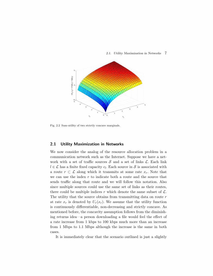
in the system, subject to resource constraints. We illustrate the sum-
utility in Figure 2.2, with the utility functions of players 1 and 2, who
receive an allocation x1 and x2 respectively being 2 log(x1) and log(x2).
The marginals in the figure are strictly concave, which results in the
sum being strictly concave as well.
2.1. Utility Maximization in Networks 7
01
23
45
0
1
2
3
4
5−5
0
5
x1
x2
U(x
1,x2)
= 2
log(
x 1) +
log(
x 2)
Fig. 2.2 Sum-utility of two strictly concave marginals.
2.1 Utility Maximization in Networks
We now consider the analog of the resource allocation problem in a
communication network such as the Internet. Suppose we have a net-
work with a set of traffic sources S and a set of links L. Each link
l ∈ L has a finite fixed capacity cl. Each source in S is associated with
a route r ⊂ L along which it transmits at some rate xr. Note that
we can use the index r to indicate both a route and the source that
sends traffic along that route and we will follow this notation. Also
since multiple sources could use the same set of links as their routes,
there could be multiple indices r which denote the same subset of L.
The utility that the source obtains from transmitting data on route r
at rate xr is denoted by Ur(xr). We assume that the utility function
is continuously differentiable, non-decreasing and strictly concave. As
mentioned before, the concavity assumption follows from the diminish-
ing returns idea—a person downloading a file would feel the effect of
a rate increase from 1 kbps to 100 kbps much more than an increase
from 1 Mbps to 1.1 Mbps although the increase is the same in both
cases.
It is immediately clear that the scenario outlined is just a slightly
8 Network Utility Maximization
more complicated version of the water resource management example
given earlier—instead of just one resource, multiple resources must be
allocated and the same amount of resource must be allocated on all
links constituting a route. It is straightforward to write down the prob-
lem as an optimization problem of the form
maxxr
∑
r∈S
Ur(xr) (2.1)
subject to the constraints
∑
r:l∈r
xr ≤ cl, ∀l ∈ L, (2.2)
xr ≥ 0, ∀r ∈ S. (2.3)
The above inequalities state that the capacity constraints of the links
cannot be violated and that each source must be allocated a non-
negative rate of transmission. It is well known that a a strictly concave
function has a unique maximum over a closed and bounded set. The
above maximization problem satisfies the requirements as the utility
function is strictly concave, and the constraint set is closed (since we
can have aggregate rate on a link equal to its capacity) and bounded
(since the capacity of every link is finite). In addition, the constraint
set for the utility maximization problem is convex which allows us to
use the method of Lagrange multipliers and the Karush-Kuhn-Tucker
(KKT) theorem which we state below [5,6].
Theorem 2.1. Consider the following optimization problem:
maxx
f(x)
subject to
gi(x) ≤ 0, ∀i = 1, 2, . . . , m,
and
hj(x) = 0, ∀j = 1, 2, . . . , l,
where x ∈ ℜn, f is a concave function, gi are convex functions and hj
are affine functions. Let x∗ be a feasible point, i.e., a point that satisfies
2.1. Utility Maximization in Networks 9
all the constraints. Suppose there exists constants λi ≥ 0 and µj such
that
∂f
∂xk(x∗)−
∑
i
λi∂gi
∂xk(x∗) +
∑
j
µj∂hj
∂xk(x∗) = 0, ∀k, (2.4)
λigi(x∗) = 0, ∀i, (2.5)
then x∗ is a global maximum. If f is strictly concave, then x∗ is also
the unique global maximum.
The constants λi and µj are called Lagrange multipliers. The KKT
conditions (2.4)-(2.5) can be interpreted as follows. Consider the La-
grangian
L(x, λ, µ) = f(x)−∑
i
λigi(x) +∑
j
µjhj(x).
Condition (2.4) is the first-order necessary condition for the maximiza-
tion problem maxx L(x, λ, µ). Further, it can be shown that the vector
of Lagrange multipliers (λ, µ) solves minλ,µ D(λ, µ) where D(λ, µ) =
maxx L(x, λ, µ) is called the Lagrange dual function.
Next, we consider an example of such a maximization problem in
a small network and show how one can solve the problem using the
above method of Lagrange multipliers.
Example 1. Consider the network in Figure 2.3 in which three sources
compete for resources in the core of the network. Links L1, L3 and L5
have a capacity of 2 units per second, while links L2 and L4 have
capacity 1 unit per second. There are three flows and denote their data
rates by x0, x1 and x2.
In our problem, links L3 and L4 are not used, while L5 does not con-
strain source S2. Assuming log utility functions, the resource allocation
problem is given by
maxx
3∑
i=0
log xi (2.6)
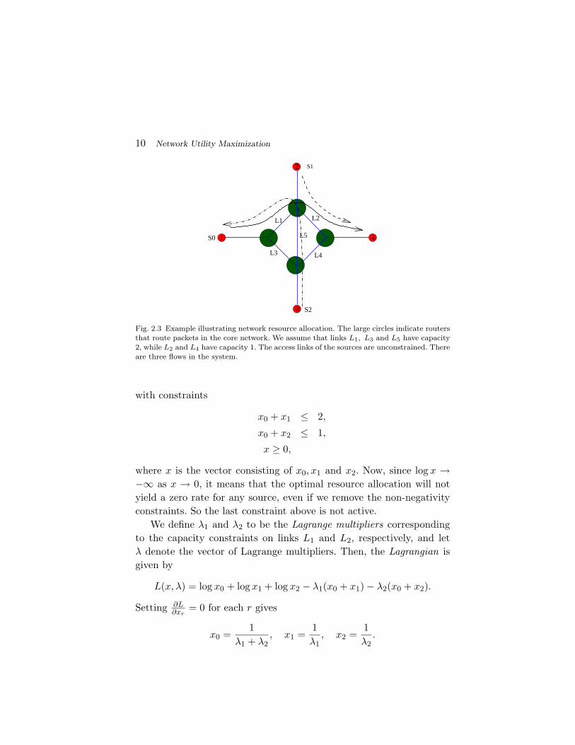
10 Network Utility Maximization
L1 L2
L5
L3 L4
1 4
3
2
S0
S1
S2
Fig. 2.3 Example illustrating network resource allocation. The large circles indicate routersthat route packets in the core network. We assume that links L1, L3 and L5 have capacity
2, while L2 and L4 have capacity 1. The access links of the sources are unconstrained. Thereare three flows in the system.
with constraints
x0 + x1 ≤ 2,
x0 + x2 ≤ 1,
x ≥ 0,
where x is the vector consisting of x0, x1 and x2. Now, since log x →−∞ as x → 0, it means that the optimal resource allocation will not
yield a zero rate for any source, even if we remove the non-negativity
constraints. So the last constraint above is not active.
We define λ1 and λ2 to be the Lagrange multipliers corresponding
to the capacity constraints on links L1 and L2, respectively, and let
λ denote the vector of Lagrange multipliers. Then, the Lagrangian is
given by
L(x, λ) = log x0 + log x1 + log x2 − λ1(x0 + x1)− λ2(x0 + x2).
Setting ∂L∂xr
= 0 for each r gives
x0 =1
λ1 + λ2, x1 =
1
λ1, x2 =
1
λ2.
2.1. Utility Maximization in Networks 11
Letting x0 + x1 = 2 and x0 + x2 = 1 (since we can always increase x2
or x3 until this is true) yields
λ1 =
√3√
3 + 1= 0.634, λ2 =
√3 = 1.732.
Note that (2.5) is automatically satisfied since x0+x1 = 2 and x0+x2 =
1. It is also possible to verify that the values of the Lagrange multipliers
actually are the minimizers of the dual function. Hence, we have the
final optimal allocation
x0 =
√3 + 1
3 + 2√
3= 0.422, x1 =
√3 + 1√
3= 1.577, x2 =
1√3
= 0.577.
A few facts are noteworthy in this simple network scenario:
• Note that x1 = 1/λ1, and it does not depend on λ2 explicitly.
Similarly, x2 does not depend on λ1 explicitly. In general, the
optimal transmission rate for source r is only determined by
the Lagrange multipliers on its route. We will later see that
this feature is extremely useful in designing decentralized al-
gorithms to reach the optimal solution.• The value of xr is inversely proportional to the sum of the
Lagrange multipliers on its route. We will see later that, in
general, xr is a decreasing function of the Lagrange multipli-
ers. Thus, the Lagrange multiplier associated with a link can
be thought of the price for using that link and the price of a
route can be thought of as the sum of the prices of its links.
If the price of a route increases, then the transmission rate
of a source using that route decreases.
In the above example, it was easy to solve the Lagrangian formula-
tion of the problem since the network was small. In the Internet which
consists of thousands of links and possibly millions of users such an
approach is not possible. In the next chapter, we will see that there
are distributed solutions to the optimization problem which are easy
to implement in the Internet.
12 Network Utility Maximization
2.2 Resource Allocation in Wireless Networks
In the previous section, we considered the case of resource allocation in
a wire-line network. Thus, we did not have to consider whether or not
a particular link would be available for transmission. This assumption
need not hold in a wireless network where scheduling one “link” for
transmission might mean that some other “link” is unavailable due
to interference. While the primary goal of this monograph is Internet
congestion control, we will briefly show how the models and methods
developed for the Internet can also be applied to wireless networks.
For ease of exposition, consider a simple model of a wireless net-
work. We model the network as a graph with a link between two nodes
indicating that the nodes are communication range of each other. When
a link is scheduled, the transmitter can transmit at a fixed rate to the
receiver. Further, a transmission from a transmitter, call it transmitter
A, to a receiver is successful if there are no other transmitters (other
than A) within a pre-specified fixed radius around the receiver. There
may be other constraints as well depending upon the details of wireless
network protocols used.
We illustrate the model in Figure 2.4. There are three flows in
progress and two of the nodes act as destinations. Around each des-
tination, we draw a circle that is called either the reception range or
interference region, depending on the context, associated with that des-
tination. A transmitter has to lie within the reception range of a receiver
for the transmission to be successful. In addition, no other node in the
interference region can transmit if the receiver is to receive the trans-
mitted data successfully. Thus, if node 2 is to successfully receive data,
either node 3 or node 1 may transmit, but not both at the same time.
In addition, many wireless networks employ an acknowledgment (ack)
protocol on each link: when a receiver successfully receives a packet,
it sends an ack back to the transmitter. Thus, for an ack to be suc-
cessful, there cannot be any transmissions within the listening range of
the transmitter as well. A transmission is not considered successful till
the transmitter receives an ack from the receiver. In Figure 2.4, if node
3 is to receive a transmission from node 2 successfully, node 1 cannot
transmit since it would interfere with the successful reception of an ack
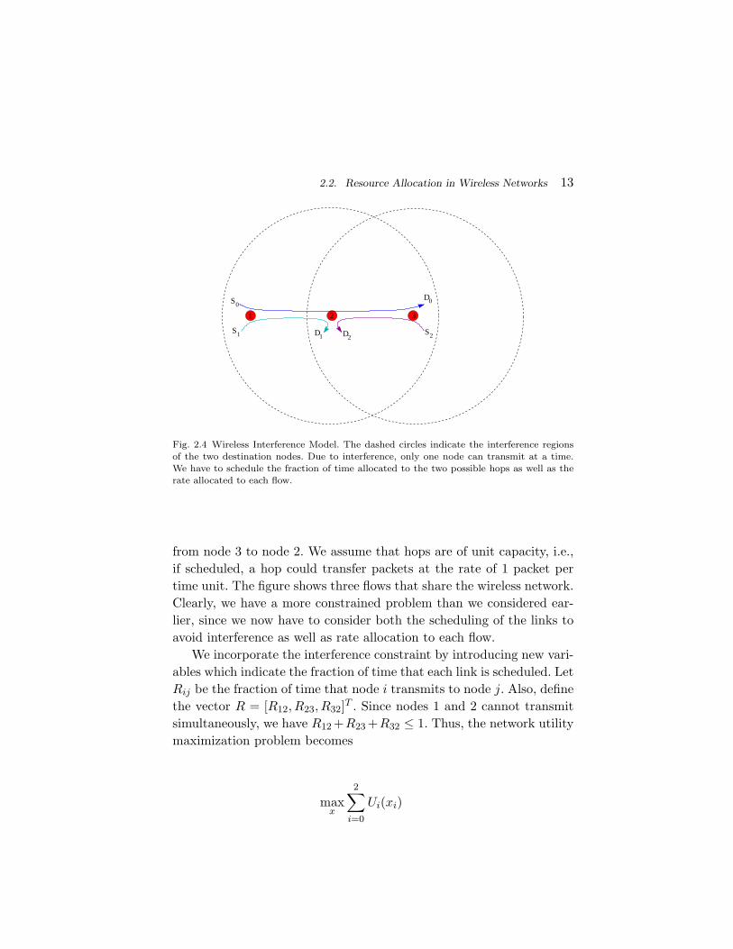
2.2. Resource Allocation in Wireless Networks 13
2S1 D
D
1 2 3
D
0
S
S 0
1 2
Fig. 2.4 Wireless Interference Model. The dashed circles indicate the interference regionsof the two destination nodes. Due to interference, only one node can transmit at a time.We have to schedule the fraction of time allocated to the two possible hops as well as the
rate allocated to each flow.
from node 3 to node 2. We assume that hops are of unit capacity, i.e.,
if scheduled, a hop could transfer packets at the rate of 1 packet per
time unit. The figure shows three flows that share the wireless network.
Clearly, we have a more constrained problem than we considered ear-
lier, since we now have to consider both the scheduling of the links to
avoid interference as well as rate allocation to each flow.
We incorporate the interference constraint by introducing new vari-
ables which indicate the fraction of time that each link is scheduled. Let
Rij be the fraction of time that node i transmits to node j. Also, define
the vector R = [R12, R23, R32]T . Since nodes 1 and 2 cannot transmit
simultaneously, we have R12 +R23 +R32 ≤ 1. Thus, the network utility
maximization problem becomes
maxx
2∑
i=0
Ui(xi)
14 Network Utility Maximization
x0 + x1 ≤ R12
x0 ≤ R23
x2 ≤ R32
R12 + R23 + R32 ≤ 1
x, R ≥ 0
We now use Lagrange multipliers to append the constraints to the
objective. Thus, we can write the dual as
maxx,R
2∑
i=0
Ui(xi)− λ1(x0 + x1 −R12)− λ2(x0 −R23)− λ3(x2 −R32)
+∑
j
γjxj − ν(R12 + R23 + R32 − 1) +∑
kl
βklRkl (2.7)
Observe (2.7) carefully. We see that there are no product terms involv-
ing x and R together. Hence we can decompose the problem into two
separate sub-problems. The first one which we call the utility maxi-
mization problem is of the form
maxx≥0
2∑
i=0
Ui(xi)− λ1(x0 + x1)− λ2x0 − λ3x2, (2.8)
while the second one which we call the scheduling problem is
maxP
kl Rkl≤1,R≥0λ1R12 + λ2R23 + λ3R32. (2.9)
Note that in writing (2.8) and (2.9), we have chosen to write some of
the constraints explicitly rather than in the Lagrange multiplier form,
but these are equivalent to the Lagrange multiplier form and are easier
to grasp intuitively.
We have seen expressions like (2.8) in the wired network example,
but did not encounter link-scheduling issues. The expression in (2.9)
uses the Lagrange multipliers (λi) as weights to determine the fractions
of time that a particular hop is scheduled. Such an algorithm to per-
form scheduling is called a maximum-weight algorithm, or max-weight
algorithm for short.
2.3. Node-Based Flow Conservation Constraints 15
2.3 Node-Based Flow Conservation Constraints
So far, we have posed the resource allocation problem as one where the
goal is to maximize network utility subject to the constraint that the
total arrival rate on each link is less than or equal to the available ca-
pacity. There is an alternative way to express the resource constraints
in the network by noting that the total arrival rate into a node must
be less than or equal to the total service rate available at the node.
From a resource allocation point of view, both formulations are equiv-
alent. However, there are subtle differences in the implementation and
analysis of decentralized algorithms required to solve the two formula-
tions. These differences will be discussed in the next chapter. As we will
see in the next chapter, these differences seem to be more important
in wireless networks and therefore, we illustrate the idea for wireless
networks.
As we did in the previous section, we now consider the example with
3 flows that was shown in Figure 2.4. Again, let the rates associated
with sources S0, S1 and S2 be x0, x1 and x2, respectively. Let R(d)ij be
the fraction of time that link (i, j) is dedicated to a flow destined for
node d. The network utility maximization problem is
maxx,R≥0
2∑
i=0
Ui(xi)
x0 ≤ R(3)12 (constraint at node 1 for destination node 3)
x1 ≤ R(2)12 (constraint at node 1 for destination node 2)
R(3)12 ≤ R
(3)23 (constraint at node 2 for destination node 3)
x2 ≤ R(2)32 (constraint at node 3 for destination node 2)
R(3)12 + R
(2)12 + R
(3)23 + R
(2)32 ≤ 1(interference and node capacity constraint).
The Lagrange dual associated with the above problem is simple to
write down, with one Lagrange multiplier λid at each node i for each
16 Network Utility Maximization
destination d (only the non-zero λid are shown below):
maxx,R≥0
2∑
i=1
Ui(xi)− λ13(x0 −R(3)12 )− λ12(x1 −R
(2)12 )
−λ23(R(3)12 −R
(3)23 )− λ32(x2 −R
(2)32 ) (2.10)
subject to
R(3)12 + R
(2)12 + R
(3)23 + R
(2)32 ≤ 1.
Now, we see again that the maximization over x and R can be split up
into two separate maximization problems:
maxx≥0
2∑
i=0
Ui(xi)− λ13x0 − λ12x1 − λ32x2 (2.11)
maxP
d,i,j Rdij≤1
R312 (λ13 − λ23) + R2
12 (λ12 − 0)
+R323 (λ23 − 0) + R2
32 (λ32 − 0) (2.12)
Note that the scheduling problem (2.12) now not only decides the
fraction of time that each hop is scheduled, but also determines the
fraction of time that a hop is dedicated to flows destined for a particular
destination. The scheduling algorithm is still a max-weight algorithm,
but the weight for each hop and each flow is now the difference in the
Lagrange multiplier at the transmitter and the Lagrange multiplier at
the receiver on the hop. This difference is called the back-pressure since
a link is not scheduled if the Lagrange multiplier at the receiver is larger
than the Lagrange multiplier at the transmitter of the hop. Thus, the
scheduling algorithm (2.12) is also called the back-pressure algorithm.
2.4 Fairness
In our discussion of the network utilization maximization, we have as-
sociated a utility function with each user. The utility function can be
viewed as a measure of satisfaction of the user when it gets a certain
data rate from the network. A different point of view is that a utility
function is assigned to each user in the network by a service provider
with the goal of achieving a certain type of resource allocation. For
2.4. Fairness 17
example, suppose U(xr) = log xr, for all users r. Then, from a well-
known property of concave functions, the optimal rates which solve
the network utility maximization problem, {xr}, satisfy
∑
r
xr − xr
xr≤ 0,
where {xr} is any other set of feasible rates. The left-hand side of the
above expression is nothing but the inner product of the gradient vector
at the optimal allocation and the vector of deviations from the optimal
allocation. This inner product is non-positive for concave functions.
For log utility functions, this property states that, under any other
allocation, the sum of proportional changes in the users’ utilities will
be non-positive. Thus, if some User A’s rate increases, then there will
be at least one other user whose rate will decrease and further, the
proportion by which it decreases will be larger than the proportion by
which the rate increases for User A. Therefore, such an allocation is
called proportionally fair. If the utilities are chosen such that Ur(xr) =
wr log xr, where wr is some weight, then the resulting allocation is said
to be weighted proportionally fair.
Another widely used fairness criterion in communication networks
is called max-min fairness. An allocation {xr} is called max-min fair if
it satisfies the following property: if there is any other allocation {xr}such a user s’s rate increases, i.e., xs > xs, then there has to be another
user u with the property
xu < xu and xu ≤ xs.
In other words, if we attempt to increase the rate for one user, then
the rate for a less-fortunate user will suffer. The definition of max-min
fairness implies that
minr
xr ≥ minr
xr,
for any other allocation {xr}. To see why this is true, suppose that
exists an allocation such that
minr
xr < minr
xr. (2.13)
This implies that, for any s such that minr xr = xs, the following holds:
xs < xs. Otherwise, our assumption (2.13) cannot hold. However, this
18 Network Utility Maximization
implies that if we switch the allocation from {xr} to {xr}, then we
have increased the allocation for s without affecting a less-fortunate
user (since there is no less-fortunate user than s under {xr}). Thus,
the max-min fair resource allocation attempts to first satisfy the needs
of the user who gets the least amount of resources from the network. In
fact, this property continues to hold if we remove all the users whose
rates are the smallest under max-min fair allocation, reduce the link
capacities by the amounts used by these users and consider the resource
allocation for the rest of the users. The same argument as above applies.
Thus, max-min is a very egalitarian notion of fairness.
Yet another form of fairness that has been discussed in the liter-
ature is called minimum potential delay fairness. Under this form of
fairness, user r is associated with the utility function −1/xr. The goal
of maximizing the sum of the user utilities is equivalent to minimizing∑
r 1/xr. The term 1/xr can be interpreted as follows: suppose user r
needs to transfer a file of unit size. Then, 1/xr is the delay in associ-
ated with completing this file transfer since the delay is simply the file
size divided by the rate allocated to user r. Hence, the name minimum
potential delay fairness.
All of the above notions of fairness can be captured by using utility
functions of the form
Ur(xr) =x1−α
r
1− α, (2.14)
for some αr > 0. Resource allocation using the above utility function
is called α-fair. Different values of α yield different ideas of fairness.
First consider α = 2. This immediately yields minimum potential delay
fairness. Next, consider the case α = 1. Clearly, the utility function
is not well-defined at this point. But it is instructive to consider the
limit α → 1. Notice that maximizing the sum of x1−αr
1−α yields the same
optimum as maximizing the sum of
x1−αr − 1
1− α.
Now, by applying L’Hospital’s rule, we get
limα→1
x1−αr − 1
1− α= log xr,
2.5. Notes 19
thus yielding proportional fairness in the limit as α → 1. Next, we
argue that the limit α → ∞ gives max-min fairness. Let xr(α) be the
α-fair allocation. Then, by the property of concave functions mentioned
at the beginning of this section,
∑
r
xr − xr
xαr
≤ 0.
Considering an arbitrary flow s, the above expression can be rewritten
as∑
r:xr≤xs
(xr − xr)xα
s
xαr
+ (xs − xs) +∑
i:xi>xs
(xi − xi)xα
s
xαi
≤ 0.
If α is very large, one would expect the third in the above expression
to be negligible. Thus, if xs > xs, then the allocation for at least one
user whose rate satisfies xr ≤ xs will decrease.
2.5 Notes
In this chapter we studied the utility maximization framework applied
to network resource allocation. When network protocols were being de-
veloped, the relationship between congestion control and fair resource
allocation was not fully understood. The idea that the congestion con-
trol is not just a means to prevent buffer overflows, but has the deeper
interpretation of allocating link bandwidths in a way that system utility
is maximized was presented in papers by Kelly et. al. [3,7–9]. The utility
maximization framework for wireless networks has been developed by
Neely et. al., Lin and Shroff, Stolyar, and Eryilmaz and Srikant [10–14].
The reader is referred to [15, 16] for more detailed surveys of the opti-
mization approach to wireless network resource allocation.
Many notions of fairness in communication networks have been pro-
posed over the years. In particular, max-min farness has been studied
extensively in [17,18]. Max-min fairness was originally developed in the
context of political philosophy by Rawls [19]. Proportional fairness was
introduced for communication networks in [3]. Nash studied this con-
cept as a bargaining solution for players bargaining over the allocation
of a common resource [20]. Hence, it is called the Nash bargaining so-
lution in economics. Minimum potential delay fairness was introduced
20 Network Utility Maximization
in [21]. The concept of α-fairness as a common framework to study
many notions of fairness was proposed by Mo and Walrand in [22,23].
In the following chapter, we will present decentralized algorithms
that converge to the solution of the network utility maximization prob-
lem.
3
Utility Maximization Algorithms
In our solution to the network utility maximization problem for a simple
network in the previous chapter, we assumed the existence of a central
authority that has complete information about all the routes and link
capacities of the network. This information was used to fairly allocate
rates to the different sources. Clearly, such a centralized solution does
not scale well when the number of sources or the number of nodes
in the network becomes large. We would like to design algorithms in
which the sources themselves perform calculations to determine their
fair rate based on some feedback from the network. We would also
like the algorithms to be such that the sources do not need very much
information about the network. How would one go about designing
such algorithms?
In this chapter we will study three such algorithms called the Pri-
mal, Dual and Primal-Dual algorithms, which derive their names from
the formulation of the optimization problem that they are associated
with. We will show how all three approaches would result in a stable
and fair allocation with simple feedback form the network. We assume
in this chapter that there are no feedback delays in the system; we
will study the effect of delays in Chapter 5. We start with the Primal
21
22 Utility Maximization Algorithms
controller, which will also serve to illustrate some basic optimization
concepts.
3.1 Primal Formulation
We relax the optimization problem in several ways so as to make algo-
rithm design tractable. The first relaxation is that instead of directly
maximizing the sum of utilities constrained by link capacities, we asso-
ciate a cost with overshooting the link capacity and maximize the sum
of utilities minus the cost. In other words, we now try to maximize
V (x) =∑
r∈S
Ur(xr)−∑
l∈L
Bl
(
∑
s:l∈s
xs
)
, (3.1)
where x is the vector of rates of all sources and Bl(.) is either a “barrier”
associated with link l which increases to infinity when the arrival rate
on a link l approaches the link capacity cl or a “penalty” function which
penalizes the arrival rate for exceeding the link capacity. By appropriate
choice of the function Bl, one can solve the exact utility optimization
problem posed in the previous chapter; for example, choose Bl(y) to be
zero if y ≤ cl and equal to ∞ if y ≥ cl. However, such a solution may
not be desirable or required. For example, the design principle may be
such that one requires the delays on all links to be small. In this case,
one may wish to heavily penalize the system if the arrival rate is larger
than say 90% of the link capacity. Losing a small fraction of the link
capacity may be considered to be quite reasonable if it improves the
quality of service seen by the users of the network since increasing the
link capacity is quite inexpensive in today’s Internet.
Another relaxation that we make is that we don’t require that
the solution of the utility maximization problem be achieved instan-
taneously. We will allow the design of dynamic algorithms that asymp-
totically (in time) approach the required maximum.
Now let us try to design an algorithm that would satisfy the above
requirements. Let us first consider the penalty function Bl(.) that ap-
pears in 3.1 above. It is reasonable to require that Bl is a convex func-
tion since we would like the penalty function to increase rapidly as we
approach or exceed the capacity. Further, assume that Bl is continu-
3.1. Primal Formulation 23
ously differentiable. Then, we can equivalently require that
Bl
(
∑
s:l∈s
xs
)
=
∫
P
s:l∈s xs
0fl(y)dy, (3.2)
where fl(.) is an increasing, continuous function. We call fl(y) the con-
gestion price function, or simply the price function, associated with
link l, since it associates a price with the level of congestion on the
link. It is straightforward to see that Bl defined in the above fashion
is convex, since integrating an increasing function results in a convex
function. If fl is differentiable, it is easy to check the convexity of Bl
since the second derivative of Bl would be positive since fl is an in-
creasing function.
Since Ur is strictly concave and Bl is convex, V (x) is strictly con-
cave. Further, we assume that Ur and fl are such that the maximization
of (3.1) results in a solution with xr ≥ 0 ∀r ∈ S. Now, the condition
that must be satisfied by the maximizer of (3.1) is obtained by differ-
entiation and is given by
U ′r(xr)−
∑
l:l∈r
fl
(
∑
s:l∈s
xs
)
= 0, r ∈ S. (3.3)
We require an algorithm that would drive x towards the solution of
(3.3). A natural candidate for such an algorithm is the gradient ascent
algorithm from optimization theory.
The idea here is that if we want to maximize a function of the from
g(x), then we progressively change x so that g(x(t + δ)) > g(x(t)).
We do this by finding the direction in which a change in x produces
the greatest increase in g(x). This direction is given by the gradient of
g(x) with regard to x. In one dimension, we merely choose the update
algorithm for x as
x(t + δ) = x(t) + k(t)dg(x)
dxδ,
where k(t) is a scaling parameter which controls the amount of change
in the direction of the gradient. Letting δ → 0
x = k(t)dg(x)
dx. (3.4)
24 Utility Maximization Algorithms
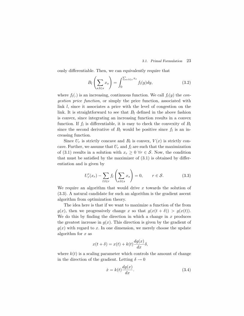
The idea is illustrated in Figure 3.1 at some selected time instants.
The value of x changes smoothly, with g(x) increasing at each time
3
1g(x)=c
g(x)=c > c2 1
g(x)=c > c2
Fig. 3.1 Gradient ascent to reach the maximum value of a function g(x). The gradient
ascent algorithm progressively climbs up the gradient so as to reach the maximum value.
instant, until it hits the maximum value.
Let us try to design a similar algorithm for the network utility
maximization problem. Consider the algorithm
xr = kr(xr)
(
U ′r(xr)−
∑
l:l∈r
fl
(
∑
s:l∈s
xs
))
, (3.5)
where kr(.) is non-negative, increasing and continuous. We have ob-
tained the above by differentiating (3.1) with respect to xr to find the
direction of ascent, and used it along with a scaling function kr(.) to
construct an algorithm of the form shown in (3.4). Clearly, the station-
ary point of the above algorithm satisfies (3.3) and hence maximizes
(3.1). The controller is called a primal algorithm since it arises from
the primal formulation of the utility maximization problem. Note that
the primal algorithm has many intuitive properties that one would ex-
pect from a resource allocation/congestion control algorithm. When
the route price qr =∑
l:l∈r fl(∑
s:l∈s xs) is large, then the congestion
controller decreases its transmission rate. Further, if xr is large, then
U ′(xr) is small (since Ur(xr) is concave) and thus the rate of increase is
small as one would expect from a resource allocation algorithm which
attempts to maximize the sum of the user utilities.
3.1. Primal Formulation 25
We must now answer two questions regarding the performance of
the primal congestion control algorithm:
• What information is required at each source in order to im-
plement the algorithm?• Does the algorithm actually converge to the desired station-
ary point?
Below we consider the answer to the first question and develop a frame-
work for answering the second. The precise answer to the convergence
question will be presented in the next sub-section.
The question of information required is easily answered by studying
(3.5). It is clear that all that the source r needs to know in order to
reach the optimal solution is the sum of the prices of each link on its
route. How would the source be appraised of the link prices? The answer
is to use a feedback mechanism—each packet generated by the source
collects the price of each link that it traverses. When the destination
receives the packet, it sends this price information in a small packet
(called the acknowledgment packet or ack packet) that it sends back
to the source.
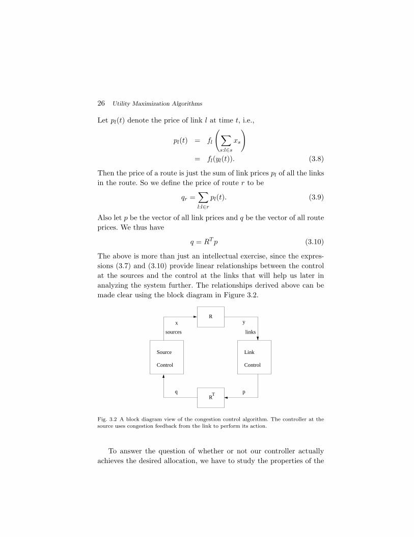
To visualize this feedback control system, we introduce a matrix R
which is called the routing matrix of the network. The (l, r) element of
this matrix is given by
Rlr =
{
1 if route r uses link l
0 else
Let us define
yl =∑
s:l∈s
xs, (3.6)
which is the load on link l. Using the elements of the routing matrix
and recalling the notation of Section 2.1, yl can also be written as
yl =∑
s:l∈s
Rlsxs.
Letting y be the vector of all yl (l ∈ L), we have
y = Rx (3.7)
26 Utility Maximization Algorithms
Let pl(t) denote the price of link l at time t, i.e.,
pl(t) = fl
(
∑
s:l∈s
xs
)
= fl(yl(t)). (3.8)
Then the price of a route is just the sum of link prices pl of all the links
in the route. So we define the price of route r to be
qr =∑
l:l∈r
pl(t). (3.9)
Also let p be the vector of all link prices and q be the vector of all route
prices. We thus have
q = RT p (3.10)
The above is more than just an intellectual exercise, since the expres-
sions (3.7) and (3.10) provide linear relationships between the control
at the sources and the control at the links that will help us later in
analyzing the system further. The relationships derived above can be
made clear using the block diagram in Figure 3.2.
links
Source
Control
Link
Control
R
RTq
x y
p
sources
Fig. 3.2 A block diagram view of the congestion control algorithm. The controller at thesource uses congestion feedback from the link to perform its action.
To answer the question of whether or not our controller actually
achieves the desired allocation, we have to study the properties of the
3.1. Primal Formulation 27
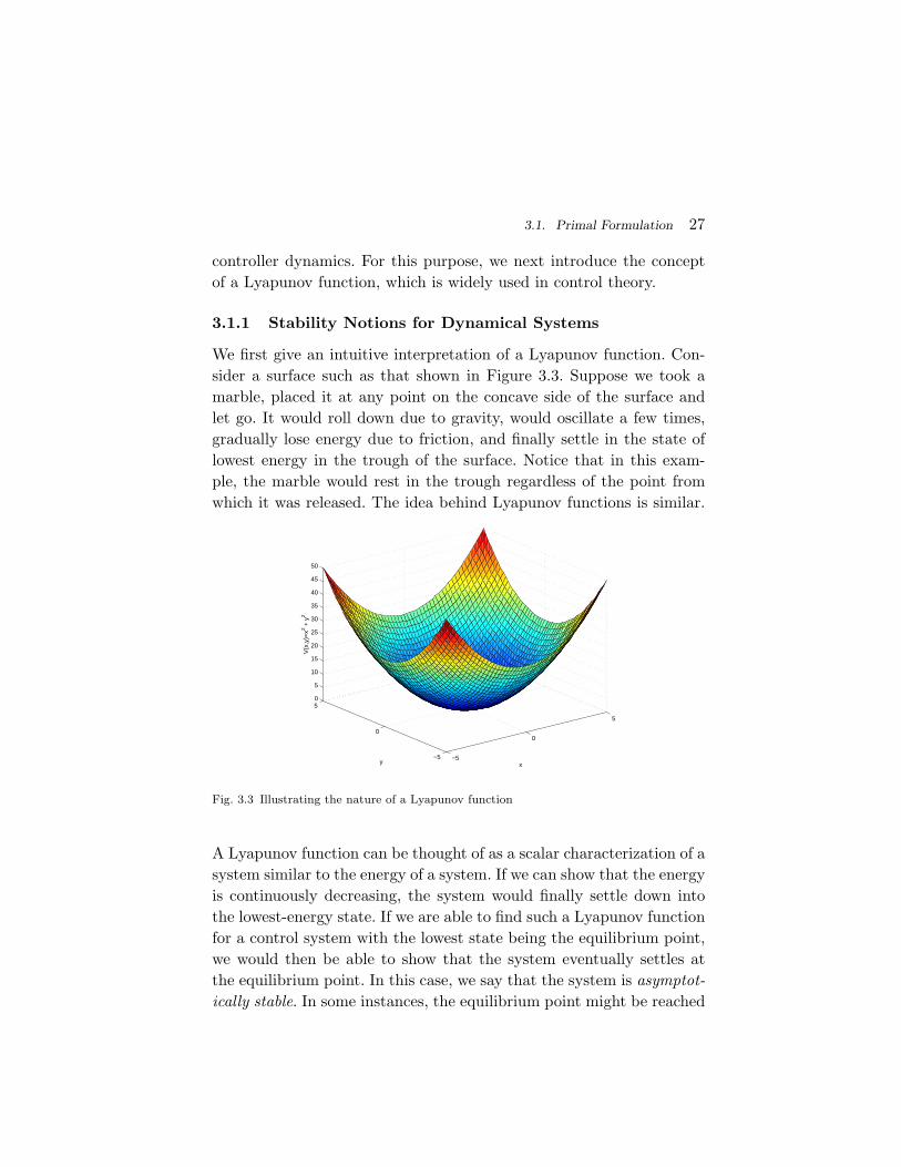
controller dynamics. For this purpose, we next introduce the concept
of a Lyapunov function, which is widely used in control theory.
3.1.1 Stability Notions for Dynamical Systems
We first give an intuitive interpretation of a Lyapunov function. Con-
sider a surface such as that shown in Figure 3.3. Suppose we took a
marble, placed it at any point on the concave side of the surface and
let go. It would roll down due to gravity, would oscillate a few times,
gradually lose energy due to friction, and finally settle in the state of
lowest energy in the trough of the surface. Notice that in this exam-
ple, the marble would rest in the trough regardless of the point from
which it was released. The idea behind Lyapunov functions is similar.
−5
0
5
−5
0
50
5
10
15
20
25
30
35
40
45
50
xy
V(x
,y)=
x2 + y
2
Fig. 3.3 Illustrating the nature of a Lyapunov function
A Lyapunov function can be thought of as a scalar characterization of a
system similar to the energy of a system. If we can show that the energy
is continuously decreasing, the system would finally settle down into
the lowest-energy state. If we are able to find such a Lyapunov function
for a control system with the lowest state being the equilibrium point,
we would then be able to show that the system eventually settles at
the equilibrium point. In this case, we say that the system is asymptot-
ically stable. In some instances, the equilibrium point might be reached
28 Utility Maximization Algorithms
only if the initial condition is in a particular set; we call such a set the
basin of attraction. If the basin of attraction is the entire state space,
then we say that the system is globally asymptotically stable. We now
formalize these intuitive ideas. Although we state the theorems under
the assumption that the equilibrium point is at zero, the results apply
even when the equilibrium is non-zero by simply shifting the coordinate
axes.
Consider a dynamical system represented by
x = g(x), x(0) = x0, (3.11)
where it is assumed that g(x) = 0 has a unique solution. Call this
solution 0. Here x and 0 can be vectors.
Definition 3.1. The equilibrium point 0 of (3.11) is said to be
• stable if, for each ε > 0, there is a δ = δ(ε) > 0, such that
‖x(t)‖ ≤ ε, ∀t ≥ 0, if ‖x0‖ ≤ δ.
• asymptotically stable if there exists a δ > 0 such that
limt→∞‖x(t)‖ = 0
for all ‖x0‖ ≤ δ.• globally, asymptotically stable if
limt→∞‖x(t)‖ = 0
for all initial conditions x0.
We now state Lyapunov’s theorem which uses the Lyapunov func-
tion to test for the stability of a dynamical system [24].
Theorem 3.1. Let x = 0 be an equilibrium point for x = f(x) and
D ⊂ Rn be a domain containing 0. Let V : D → R be a continuously
differentiable function such that
V (x) > 0, ∀x 6= 0
and V (0) = 0. Now we have the following conditions for the various
notions of stability.
3.1. Primal Formulation 29
(1) If V (x) ≤ 0 ∀x, then the equilibrium point is stable.
(2) In addition, if V (x) < 0, ∀x 6= 0, then the equilibrium point
is asymptotically stable.
(3) In addition to (1) and (2) above, if V is radially unbounded,
i.e.,
V (x)→∞, when ‖x‖ → ∞,
then the equilibrium point is globally asymptotically stable.
Note that the above theorem also holds if the equilibrium point is
some x 6= 0. In this case, consider a system with state vector y = x− x
and the results immediately apply.
3.1.2 Global Asymptotic Stability of the Primal Controller
We show that the primal controller of (3.5) is globally asymptotically
stable by using the Lyapunov function idea described above. Recall that
V (x) as defined in 3.1 is a strictly concave function. Let x be its unique
maximum. Then, V (x)−V (x) is non-negative and is equal to zero only
at x = x. Thus, V (x)−V (x) is a natural candidate Lyapunov function
for the system (3.5). We use this Lyapunov function in the following
theorem.
Theorem 3.2. Consider a network in which all sources follow the pri-
mal control algorithm (3.5). Assume that the functions Ur(.), kr(.) and
fl(.) are such that W (x) = V (x) − V (x) is such that W (x) → ∞ as
||x|| → ∞, xi > 0 for all i, and V (x) is as defined in (3.1). Then, the
controller in (3.5) is globally asymptotically stable and the equilibrium
value maximizes (3.1).
Proof. Differentiating W (.), we get
W = −∑
r∈S
∂V
∂xrxr = −
∑
r∈S
kr(xr)(
U ′r(xr)− qr
)2< 0, ∀x 6= x, (3.12)
and W = ∀x = x. Thus, all the conditions of the Lyapunov theorem
are satisfied and we have proved that the system state converges to x.
30 Utility Maximization Algorithms
In the proof of the above theorem, we have assumed that utility,
price and scaling functions are such that W (x) has some desired prop-
erties. It is very easy to find functions that satisfy these properties.
For example, if Ur(xr) = wr log(xr), and kr(xr) = xr, then the primal
congestion control algorithm for source r becomes
xr = wr − xr
∑
l:l∈r
fl(yl),
and thus the unique equilibrium point is wr/xr =∑
l:l∈r fl(yl). If fl(.)
is any polynomial function, then V (x) goes to −∞ as ||x|| → ∞ and
thus, W (x)→∞ as ||x|| → ∞.
3.1.3 Price Functions and Congestion Feedback
We had earlier argued that collecting the price information from the
network is simple. If there is a field in the packet header to store price
information, then each link on the route of a packet simply adds its
price to this field, which is then echoed back to source by the receiver
in the acknowledgment packet. However, packet headers in the Internet
are already crowded with a lot of other information, so Internet prac-
titioners do not like to add many bits in the packet header to collect
congestion information. Let us consider the extreme case where there is
only one bit available in the packet header to collect congestion infor-
mation. How could we use this bit to collect the price of route? Suppose
that each packet is marked with probability 1− e−pl when the packet
passes through link l. Marking simply means that a bit in the packet
header is flipped from a 0 to a 1 to indicate congestion. Then, along a
route r, a packet is marked with probability
1− eP
l:l∈r pl .
If the acknowledgment for each packet contains one bit of information
to indicate if a packet is marked or not, then by computing the fraction
of marked packets, the source can compute the route price∑
l:l∈r pl.
The assumption here is that the congestion control occurs at a slower
time-scale than the packet dynamics in the network so that pl remains
roughly a constant over many packets.
3.1. Primal Formulation 31
Price functions were assumed to be functions of the arrival rate at
a link. However, in practice, it is quite common to indicate congestion
based on the queue length at a link. For example, consider the follow-
ing congestion notification mechanism. Whenever the queue length at
a node exceeds a threshold B at the time of a packet arrival, then the
packet is marked. For the moment assume that there is only one link in
the network. Further, again suppose that the congestion controller acts
at a slower time compared to the queue length dynamics. For example,
the congestion controller may react to the fraction of packets marked
over a time interval. In this case, one can roughly view the price func-
tion for the link as the fraction of marked packets. To compute the
fraction of marked packets, one needs a model for the packet arrival
process at the link which could, in general, be a stochastic process. For
simplicity, assume that the arrival process is a Poisson process of rate yl
which remains constant compared to the time-scale of the congestion
control process. Further, suppose that packet sizes are exponentially
distributed. Then, the fraction of marked packets is simply the prob-
ability that the number of packets in an M/M/1/ queue exceeds B,
which is given by pl = fl(yl) = (yl/cl)B if yl < cl and is equal to 1
otherwise [18]. If there is only one bit in the packet header to indicate
congestion, then a packet is marked if it is marked on any one of the
links on its route. Thus, the packet marking probability on a route r is
given by 1−∏l:l∈r(1−pl). If the pl are small, then one can approximate
the above by∑
l∈r pl, which is consistent with the primal formulation
of the problem.
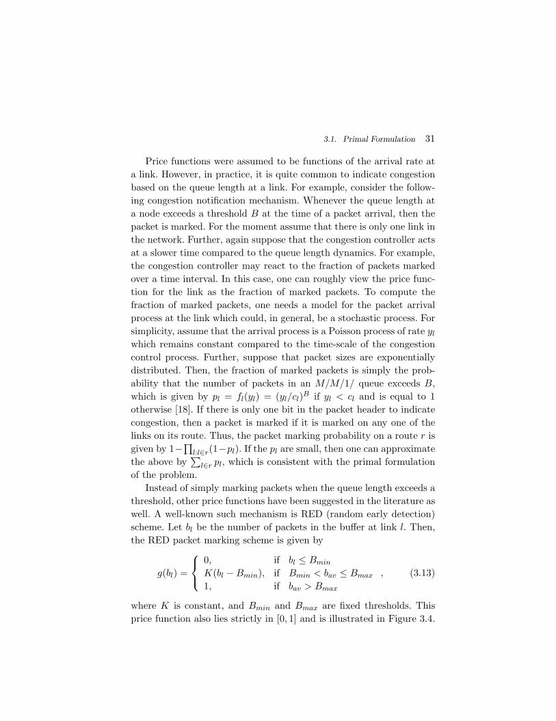
Instead of simply marking packets when the queue length exceeds a
threshold, other price functions have been suggested in the literature as
well. A well-known such mechanism is RED (random early detection)
scheme. Let bl be the number of packets in the buffer at link l. Then,
the RED packet marking scheme is given by
g(bl) =
0, if bl ≤ Bmin
K(bl −Bmin), if Bmin < bav ≤ Bmax
1, if bav > Bmax
, (3.13)
where K is constant, and Bmin and Bmax are fixed thresholds. This
price function also lies strictly in [0, 1] and is illustrated in Figure 3.4.
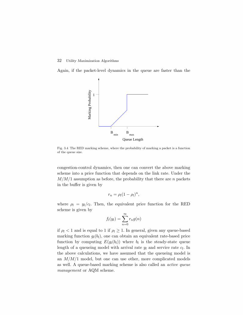
32 Utility Maximization Algorithms
Again, if the packet-level dynamics in the queue are faster than the
Queue Lengthmin
Bmax
1
Mar
king
Pro
babi
lity
B
Fig. 3.4 The RED marking scheme, where the probability of marking a packet is a functionof the queue size.
congestion-control dynamics, then one can convert the above marking
scheme into a price function that depends on the link rate. Under the
M/M/1 assumption as before, the probability that there are n packets
in the buffer is given by
rn = ρl(1− ρl)n,
where ρl = yl/cl. Then, the equivalent price function for the RED
scheme is given by
fl(yl) =∞∑
n=0
rng(n)
if ρl < 1 and is equal to 1 if ρl ≥ 1. In general, given any queue-based
marking function gl(bl), one can obtain an equivalent rate-based price
function by computing E(gl(bl)) where bl is the steady-state queue
length of a queueing model with arrival rate yl and service rate cl. In
the above calculations, we have assumed that the queueing model is
an M/M/1 model, but one can use other, more complicated models
as well. A queue-based marking scheme is also called an active queue
management or AQM scheme.
3.2. Dual Formulation 33
Another price function of interest is found by considering packet
dropping instead of packet marking. If packets are dropped due to the
fact that a link buffer is full when a packet arrives at the link, then such
a dropping mechanism is called a Droptail scheme. Assuming Poisson
arrivals and exponentially distributed file sizes, the probability that a
packet is dropped when the buffer size is B is given by
1− ρ
1− ρB+1ρB,
where ρ =P
r:l∈ r xr
cl. As the number of users of the Internet increases,
one might conceivably increase the buffer sizes as well in proportion,
thus maintaining a constant maximum delay at each link. In this case,
B →∞ would be a reasonable approximation. We then have
limB→∞
1− ρ
1− ρB+1ρB =
{
0, if ρ < 1,
1− 1ρ , if ρ ≥ 1.
Thus, an approximation for the drop probability is(
1− 1ρ
)+, which is
non-zero only if∑
r:l∈ r xr is larger than cl. When packets are dropped
at a link for source r, then the arrival rate from source r at the next
link on the link would be smaller due to the fact that dropped packets
cannot arrive at the next link. Thus, the arrival rate is “thinned” as
we traverse the route. However, this is very difficult to model in our
optimization framework. Thus, the optimization is valid only if the
drop probability is small. Further, the end-to-end drop probability on
a route can be approximated by the sum of the drop probabilities on
the links along the route if the drop probability at each link is small.
We now move on to another class of resource allocation algorithms
called Dual Algorithms. All the tools we have developed for studying
primal algorithms will be used in the dual formulation as well.
3.2 Dual Formulation
In the previous section, we studied how to design a stable and simple
control mechanism to asymptotically solve the relaxed utility maxi-
mization problem. We also mentioned that by using an appropriate
34 Utility Maximization Algorithms
barrier function, one could obtain the exact value of the optimal so-
lution. In this section we consider a different kind of controller based
on the dual formulation of the utility maximization problem that nat-
urally produces the optimal solution without any relaxation. Consider
the resource allocation problem that we would like to solve
maxxr
∑
r∈S
Ur(xr) (3.14)
subject to the constraints∑
r:l∈r
xr ≤ cl, ∀l ∈ L, (3.15)
xr ≥ 0, ∀r ∈ S. (3.16)
The Lagrange dual of the above problem is obtained by incorporating
the constraints into the maximization by means of Lagrange multipliers
as follows:
D(p) = max{xr>0}
∑
r
Ur(xr)−∑
l
pl
(
∑
s:l∈s
xs − cl
)
(3.17)
Here the pls are the Lagrange multipliers that we saw in the previous
chapter. The dual problem may then be stated as
minp≥0
D(p).
As in the case of the primal problem, we would like to design an
algorithm that causes all the rates to converge to the optimal solution.
Notice that in this case we are looking for a gradient descent (rather
than a gradient ascent that we saw in the primal formulation), since
we would like to minimize D(p). To find the direction of the gradient,
we need to know ∂D∂pl
.
We first observe that in order to achieve the maximum in (3.17), xr
must satisfy
U ′r(xr) = qr, (3.18)
or equivalently,
xr = U ′r−1
(qr), (3.19)
3.2. Dual Formulation 35
where, as usual, qr =∑
l:l∈r pr, is the price of a particular route r. Now,
since∂D
∂pl=∑
r:l∈r
∂D
∂qr
∂qr
∂pl,
we have from (3.19) and (3.17) that
∂D
∂pl=∑
r:l∈r
∂Ur(xr)
∂pl− (yl − cl)−
∑
i
pi∂yi
∂pl, (3.20)
where the xr above is the optimizing xr in (3.17). In order to evaluate
the above, we first compute ∂xr/∂pl. Differentiating (3.18) with respect
to pl yields
U ′′r (xr)
dxr
dpl= 1
⇒ ∂xr
∂pl=
1
U ′′r (xr)
Substituting the above in (3.20) yields
∂D
∂pl=
∑
r:l∈r
U ′r(xr)
U ′′r (xr)
− (yl − cl)−∑
i
pi
∑
r:l∈r
1
U ′′r (xr)
(3.21)
= cl − yl, (3.22)
where we have interchanged the last two summations in (3.21) and used
the facts U ′r(xr) = qr and qr =
∑
l∈r pl. The above is the gradient of
the Lagrange dual, i.e., the direction in which it increases. We are now
ready to design our controller. Recalling that we need to descend down
the gradient, from (3.19) and (3.22), we have the following dual control
algorithm:
xr = U ′r−1
(qr) and (3.23)
pl = hl(yl − cl)+pl
, (3.24)
where, hl > 0 is a constant and (g(x))+y denotes
(g(x))+y =
{
g(x), y > 0,
max(g(x), 0), y = 0,
We use this modification to ensure that pl never goes negative since we
know from the KKT conditions that the optimal price is non-negative.
36 Utility Maximization Algorithms
Note that, if hl = 1, the price update above has the same dynamics
as the dynamics of the queue at link l. The price increases when the
arrival rate is larger than the capacity and decreases when the arrival
rate is less than the capacity. Moreover, the price can never become
negative. These are exactly the same dynamics that govern the queue
size at link l. Thus, one doesn’t even have to explicitly keep track of
the price in the dual formulation; the queue length naturally provides
this information. However, there is a caveat. We have assumed that the
arrivals from a source arrive to all queues on the path simultaneously.
In reality the packets must go through the queue at one link before
arriving at the queue at the next link. There are two ways to deal with
this issue:
• Assume that the capacity cl is not the true capacity of a link,
but is a fictitious capacity which is slightly less than the true
capacity. Then, ql will be the length of this virtual queue
with the virtual capacity cl. A separate counter must then
be maintained to keep track of the virtual queue size, which
is the price of the link. Note that this price must be fed back
to the sources. Since the congestion control algorithm reacts
to the virtual queue size, the arrival rate at the link will be
at most cl and thus will be less than the true capacity. As a
result, the real queue size at the link would be negligible. In
this case, one can reasonably assume that packets move from
link to link without experiencing significant queueing delays.• Once can modify the queueing dynamics to take into account
the route traversal of the packets. We will do so in a later
section on the primal-dual algorithm. This modification may
be more important in wireless networks where interference
among various links necessitates scheduling of links and thus,
a link may not be scheduled for a certain amount of time.
Therefore, packets will have to wait in a queue till they are
scheduled and thus, we will model the queueing phenomena
precisely.
3.2. Dual Formulation 37
3.2.1 Stability of the Dual Algorithm
Since we designed the dual controller in much the same way as the
primal controller and they both are gradient algorithms (ascent in one
case and descent in the other), we would expect that the dual algorithm
too will converge to the optimal solution. We show using Lyapunov
theory that this is indeed the case.
We first understand the properties of the solution of the original
network utility maximization problem (2.1). Due to the same concavity
arguments used earlier, we know that the maximizer of (2.1) which we
denote by x is unique. Suppose also that in the dual formulation (3.17)
given q, there exists a unique p such that q = RT p (i.e., R has full row
rank), where R is the routing matrix. At the optimal solution
q = RT p,
and the KKT conditions imply that, at each link l, either
yl = cl
if the constraint is active or
yl < cl and pl = 0
if the link is not a fully utilized. Note that under the full row rank
assumption on R, p is also unique.
Theorem 3.3. Under the assumption that given q, there exists a
unique p such that q = RT p, the dual algorithm is globally asymp-
totically stable.
Proof. Consider the Lyapunov function
V (p) =∑
l∈L
(cl − yl)pl +∑
r∈S
∫ qr
qr
(xr − (U ′r)
−1(σ))dσ.
38 Utility Maximization Algorithms
Then we have
dV
dt=
∑
l
(cl − yl)pl +∑
r
(xr − (U ′r)
−1(qr))qr
= (c− y)T p + (x− x)T q
= (c− y)T p + (x− x)T RT p
= (c− y)T p + (y − y)T p
= (c− y)T p
=∑
l
hl(cl − yl)(yl − cl)+pl
≤ 0.
Also, V = 0 only when each link satisfies either yl = cl or yl < cl
with pl = 0. Further, since U ′r(xr) = qr at each time instant, thus all
the KKT conditions are satisfied. The system converges to the unique
optimal solution of (2.1).
3.3 Extension to Multi-path Routing
The approaches considered in this chapter can be extended to account
for the fact that there could be multiple routes between each source-
destination pair. The existing protocols on the Internet today do not
allow the use of multiple routes, but it is not hard to envisage a situation
in the future where smart routers or overlay routers would allow such
routing. Our goal is to find an implementable, decentralized congestion
control algorithm for such a network with multi-path routing. Figure
3.5 indicates a simple scenario where this might be possible.
As before, the set of sources is called S. Each source s ∈ S identifies
a unique source-destination pair. Also, each source may use several
routes. If source s is allowed to use route r, we say r ∈ s. Similarly,
if a route r uses link j, we say j ∈ r. For each route r we let s(r)
be the unique source such that r ∈ s(r). We call the set of routes
R. As in single-path routing, note that two paths in the network that
are otherwise identical can be associated with two different indices
r ∈ R, if their sources are different. For instance, in Figure 3.5 suppose
there were two sources s1 and s3 between the node pair (N1, N3). Let
s1 subscribe to the multi-path service. Then the collection of routes
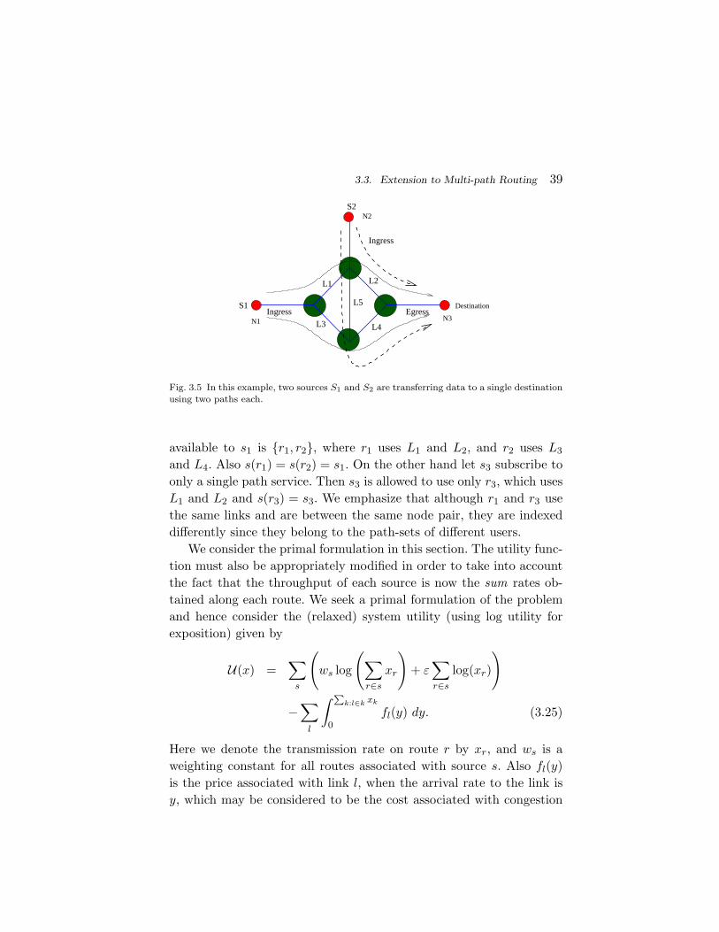
3.3. Extension to Multi-path Routing 39
N3
N2
N1
DestinationEgress
S2
S1
L4L3
L5
L2L1
Ingress
Ingress
Fig. 3.5 In this example, two sources S1 and S2 are transferring data to a single destinationusing two paths each.
available to s1 is {r1, r2}, where r1 uses L1 and L2, and r2 uses L3
and L4. Also s(r1) = s(r2) = s1. On the other hand let s3 subscribe to
only a single path service. Then s3 is allowed to use only r3, which uses
L1 and L2 and s(r3) = s3. We emphasize that although r1 and r3 use
the same links and are between the same node pair, they are indexed
differently since they belong to the path-sets of different users.
We consider the primal formulation in this section. The utility func-
tion must also be appropriately modified in order to take into account
the fact that the throughput of each source is now the sum rates ob-
tained along each route. We seek a primal formulation of the problem
and hence consider the (relaxed) system utility (using log utility for
exposition) given by
U(x) =∑
s
(
ws log
(
∑
r∈s
xr
)
+ ε∑
r∈s
log(xr)
)
−∑
l
∫
P
k:l∈k xk
0fl(y) dy. (3.25)
Here we denote the transmission rate on route r by xr, and ws is a
weighting constant for all routes associated with source s. Also fl(y)
is the price associated with link l, when the arrival rate to the link is
y, which may be considered to be the cost associated with congestion
40 Utility Maximization Algorithms
on the link y. Note that we have added a term containing ε to ensure
that the net utility function is strictly concave and hence has a unique
maximum. The presence of the ε term also ensures that a non-zero rate
is used on all paths allowing us automatically to probe the price on all
paths. Otherwise, an additional probing protocol would be required to
probe each high-price path to know when its price drops significantly
to allow transmission on the path.
We then consider the following controller, which is a natural gen-
eralization of the earlier single-path controller to control the flow on
route r:
xr(t) = κrxr
wr −
∑
m∈s(r)
xm(t)
qr(t)
+κrε∑
m∈s(r)
xm(t), (3.26)
where wr = ws for all routes r associated with source s. The term qr(t)
is the estimate of the route price at time t. This price is the sum of the
individual link prices pl on that route. The link price in turn is some
function fl of the arrival rate at the link. The fact that the controller
is globally asymptotically stable can be shown as we did in the primal
formulation using U(x)−U(x) as the Lyapunov function. The proof is
identical to the one presented earlier and hence will not be repeated
here.
So far, we have seen two types of controllers for the wired Internet,
corresponding to the primal and dual approaches to constrained opti-
mization. We will now study a combination of both controllers called
the primal-dual controller in the more general setting of a wireless
network. The wireless setting is more general since the case of the In-
ternet is a special case where there are no interference constraints. It
is becoming increasingly clear that significant portions of the Inter-
net are evolving towards wireless components; examples include data
access through cellular phones, wireless LANs and multi-hop wireless
networks which are widely prevalent in military, law enforcement and
emergency response networks, and which are expected to become com-
mon in the civilian domain at least in certain niche markets such as
3.4. Primal-Dual Algorithm for Wireless Networks 41
viewing replays during football games, concerts, etc. As mentioned in
the previous chapter, our goal here is not to provide a comprehensive
introduction to resource allocation in wireless networks. Our purpose
here is to point out that the simple fluid model approach that we have
taken so far extends to wireless networks at least in establishing the
stability of congestion control algorithms. On the other hand, detailed
scheduling decisions require more detailed models which we do not con-
sider here.
3.4 Primal-Dual Algorithm for Wireless Networks
In the discussion thus far, we saw that both controllers use rate-update
functions at the source side, and price-update functions on each of
the links. The exact form of the updates were different in the two
cases. It is possible to combine the two controllers by using the rate-
update from the primal and the price-update from the dual. Such a
controller is called a primal-dual controller. While we could illustrate
such a controller in the same wired-network setting as above, we will
do so for a wireless network in this section.
Let N be the set of nodes and L be the set of permissible hops. Let
F be the set of flows in the system. We do not associate flows with
fixed routes, but routes would also be decided by the resource alloca-
tion algorithm. In principle, all flows could potentially use all nodes
in the system as part of their routes. Of course, the results also ap-
ply to the special case where a route is associated with a flow. Each
flow f has a beginning node b(f) and an ending node e(f). We assume
that each node maintains a separate queue for each source-destination
pair. Let rij be the rate at which transmission takes place from node
i to node j. Due to interference, the rates between the various nodes
are inter-related. We consider a simple model to describe this inter-
ference although the results can be generalized significantly. Let {Am}m = 1, 2, . . . , M be a collection of subsets of L. The set Am is a set
of hops that can be scheduled simultaneously given some interference
constraints. Each Am is called a feasible schedule and M is the number
of possible feasible schedules. If schedule Am is used, then rij = 1 if
(i, j) ∈ Am, and rij = 0 otherwise. Thus, all the scheduled links can
42 Utility Maximization Algorithms
transmit at rate 1 while the unscheduled hops remain silent. The net-
work has a choice of implementing any one of the schedules at each
time instant. Suppose that πm is the fraction of time that the network
chooses to use schedule m. Then, the average rate allocated to hop
(i, j) is given by
Rij =∑
m:(i,j)∈Am
πm.
In this section, we will use the node-based resource constraint formu-
lation used in Section 2.3. Thus, at each node, we keep track of the
rate at which traffic arrives and leaves for a particular destination, and
impose the constraint that the arrival rate is less than the departure
rate. The reason we choose this formulation is that we will maintain a
separate queue for each destination at each node, and the constraints
ensure that each of the per-destination queues is stable. We will see
that, under this formulation, one does not have to assume that arrivals
occur to each queue along a path simultaneously as in the previous sec-
tion. To formulate the node-based constraints, denote the inflow rate
allocated for destination d at node i by Rdin(i) and the outflow rate
Rdout(i). Thus, at each node i,
∑
d
Rdin(i) =
∑
j
Rji and∑
d
Rdout(i) =
∑
k
Rik.
For simplicity, we will only consider the case where Ur(xr) =
wr log xr. Thus, the optimization problem for the resource allocation
problem is given by
maxx,π,R≥0
∑
f
wf log xf ,
3.4. Primal-Dual Algorithm for Wireless Networks 43
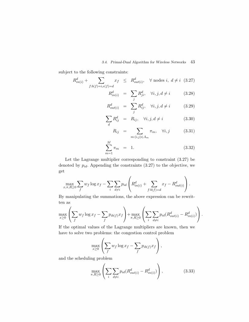
subject to the following constraints:
Rdin(i) +
∑
f :b(f)=i,e(f)=d
xf ≤ Rdout(i), ∀ nodes i, d 6= i (3.27)
Rdin(i) =
∑
j
Rdji, ∀i, j, d 6= i (3.28)
Rdout(i) =
∑
j
Rdij , ∀i, j, d 6= i (3.29)
∑
d
Rdij = Rij , ∀i, j, d 6= i (3.30)
Rij =∑
m:(i,j)∈Am
πm, ∀i, j (3.31)
M∑
m=1
πm = 1. (3.32)
Let the Lagrange multiplier corresponding to constraint (3.27) be
denoted by pid. Appending the constraints (3.27) to the objective, we
get
maxx,π,R≥0
∑
f
wf log xf −∑
i
∑
d6=i
pid
Rdin(i) +
∑
f :b(f)=d
xf −Rdout(i)
.
By manipulating the summations, the above expression can be rewrit-
ten as
maxx≥0
∑
f
wf log xf −∑
f
pib(f)xf
+ maxπ,R≥0
∑
i
∑
d6=i
pid(Rdout(i) −Rd
in(i))
.
If the optimal values of the Lagrange multipliers are known, then we
have to solve two problems: the congestion control problem
maxx≥0
∑
f
wf log xf −∑
f
pib(f)xf
,
and the scheduling problem
maxπ,R≥0
∑
i
∑
d6=i
pid(Rdout(i) −Rd
in(i))
, (3.33)
44 Utility Maximization Algorithms
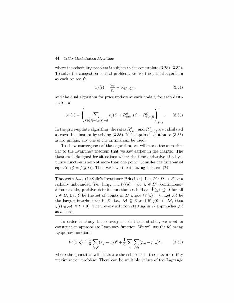
where the scheduling problem is subject to the constraints (3.28)-(3.32).
To solve the congestion control problem, we use the primal algorithm
at each source f :
xf (t) =wr
xr− pb(f)e(f), (3.34)
and the dual algorithm for price update at each node i, for each desti-
nation d:
pid(t) =
∑
f :b(f)=i,e(f)=d
xf (t) + Rdin(i)(t)−Rd
out(i)
+
pnd
. (3.35)
In the price-update algorithm, the rates Rdin(i) and Rd
out(i) are calculated
at each time instant by solving (3.33). If the optimal solution to (3.33)
is not unique, any one of the optima can be used.
To show convergence of the algorithm, we will use a theorem sim-
ilar to the Lyapunov theorem that we saw earlier in the chapter. The
theorem is designed for situations where the time-derivative of a Lya-
punov function is zero at more than one point. Consider the differential
equation y = f(y(t)). Then we have the following theorem [24]:
Theorem 3.4. (LaSalle’s Invariance Principle). Let W : D → R be a
radially unbounded (i.e., lim||y||→∞ W (y) = ∞, y ∈ D), continuously
differentiable, positive definite function such that W (y) ≤ 0 for all
y ∈ D. Let E be the set of points in D where W (y) = 0. Let M be
the largest invariant set in E (i.e., M ⊆ E and if y(0) ∈ M, then
y(t) ∈ M ∀ t ≥ 0). Then, every solution starting in D approaches Mas t→∞.
In order to study the convergence of the controller, we need to
construct an appropriate Lyapunov function. We will use the following
Lyapunov function:
W (x, q) ,1
2
∑
f∈F
(xf − xf )2 +1
2
∑
i
∑
d6=i
(pid − pnd)2, (3.36)
where the quantities with hats are the solutions to the network utility
maximization problem. There can be multiple values of the Lagrange
3.4. Primal-Dual Algorithm for Wireless Networks 45
multipliers that satisfy the KKT conditions; in that case, one can pick
any one of them to construct the Lyapunov function. From now on, in
double summations involving a node i and destination d, for ease of
notation, we will assume that d 6= i without explicitly stating it. We
are now ready to prove the following theorem:
Theorem 3.5. Starting from any x(0) and q(0), the rate vector x(t)
converges to x as t→∞ and
pb(f)e(f) = pb(f)e(f) = wf/xf ∀ f.
Further, the queue length vector p(t) approaches the bounded set
p ≥ 0 :∑
i,d
(pid − pid)
Rdout(i) −Rd
in(i) +∑
f :b(f)=i,e(f)=d
(xf − xf )
= 0
.
Proof. Differentiating the Lyapunov function with respect to time we
obtain
W =∑
f
(xf − xf )
(
1
xf− pb(f)e(f)
)
+∑
i,d
(pid − pid)
∑
f :b(f)=i,e(f)=d
xf + Rdin(i) −Rd
out(i)
+
pid
(3.37)
≤∑
f
(xf − xf )(1
xf− pb(f)e(f))
+∑
i,d
(pid − pid)
∑
f :b(f)=i,e(f)=d
xf + Rdin(i) −Rd
out(i)
.(3.38)
The last inequality follows by noting that (3.38) and (3.37) are equal
if the projection in (3.37) is inactive and if the projection is active, the
expression in (3.37) is zero, while the expression in (3.38) is positive
due to the fact that pid = 0 and the term inside the parenthesis is
negative (otherwise, the projection will not be active). Using the fact
46 Utility Maximization Algorithms
wf/xf = pb(f)e(f) and adding and subtracting terms, we get
W =∑
f
(xf − xf )
(
1
xf− 1
xf+ pb(f)e(f) − pb(f)e(f)
)
+∑
i,d
(pid − pid)
∑
f :b(f)=i,e(f)=d
xf −∑
f :b(f)=i
xf
+∑
i,d
(pid − pid)
∑
f :b(f)=i,e(f)=d
xf + Rdin(i) −Rd
out(i)
.
Noting that∑
i,d
(pid−pid)∑
f :b(f)=i,e(f)=d
(xf−xf ) = −∑
f
(xf−xf )(pb(f)e(f)−pb(f)e(f)),
we get
W =∑
f
(xf − xf )(1
xf− 1
xf)
+∑
i,d
(pid − pid)
∑
f :b(f)=i,e(f)=d
xf + Rdin(i) −Rd
out(i)
.
Let us now examine each of the terms in the right-hand side of the
above equation. It is easy to see that
(xf − xf )(1
xf− 1
xf) ≤ 0.
From constraint (3.27),∑
f :b(f)=i,e(f)=d
xf ≤ Rdout(i) − Rd
in(i),
where we recall that the quantities with hats are the optimal solution
to the network utility maximization problem. Thus,
∑
i,d
pid
∑
f :b(f)=i,e(f)=d
xf + Rdin(i) −Rd
out(i)
≤ 0,
3.4. Primal-Dual Algorithm for Wireless Networks 47
since the rates Rdin(i) and Rd
out(i) solve (3.33) and Rdout(i) and Rd
in(i)
are feasible solutions to the outflow and inflow rates at node i, for
destination d. From the KKT conditions
pid
Rdin(i) +
∑
f :b(f)=i,e(f)=d
xf − Rdout(i)
= 0.
Thus,
−∑
i,d
pid
∑
f :b(f)=i,e(f)=d
xf + Rdin(i) −Rd
out(i)
= −∑
i,d
pid
∑
f :b(f)=i,e(f)=d
Rdout(i) − Rd
in(i) −Rdout(i) + Rd
in(i)
≤ 0,
since the R’s solve the scheduling problem with p’s as the weights in
the scheduling algorithm. Thus, W ≤ 0. To apply LaSalle’s invariance
principle, let us consider the set of points E , where W = 0. The set Eis given by the set of points (x, p) that satisfy
xf = xf ,∑
i,d
(pid − pid)
∑
f :b(f)=i,e(f)=d
xf + Rdin(i) −Rd
out(i)
= 0
.
We claim that the largest invariant setM⊆ E is further characterized
by pb(f)e(f) = wf/xf . To see this, note that if this condition is violated,
then the congestion controller (3.34) will change the rate from xf and
hence the system will move outside E . Thus, LaSalle’s invariance prin-
ciple applies and the theorem is proved.
We will now examine the scheduling problem (3.33) carefully with
the goal of simplifying it. By rearranging the summation and using the
definitions of Rdin(i) from (3.28) and Rd
out(i) from (3.29), (3.33) can be
rewritten as
max∑
i,k
∑
d
Rdik(pid − pkd).
Using the fact that∑
d Rdik = Rik, the scheduling problem becomes
max∑
i,k
Rik maxd
(pid − pkd).
48 Utility Maximization Algorithms
Using (3.31) and (3.32), the scheduling problem further reduces to
maxP
m πm=1
∑
i,k,m:(i,k)∈Am
πm maxd
(pid − pkd) (3.39)
= maxP
m πm=1
∑
m
πm
∑
(i,k)∈Am
maxd
(pid − pkd)
= maxm
∑
(i,k)∈Am
maxd
(pid − pkd). (3.40)
Thus, the scheduling problem becomes one of finding a schedule with
the maximum weight, where the weight of a link is given by
maxd
(pid − pkd).
This is called the back-pressure algorithm.
Let us examine the price-update equation (3.35). This equation
closely resembles the queue dynamics in the queue holding packets for
destination d at packet i. However, notice that the arrival rate into the
queue includes the term
Rdin(i) =
∑
j
Rdji,
which is not the true arrival rate at the queue, but it is the potential
rate at which packets could arrive from other nodes to node i. This rate
may not be realizable if some of the other nodes have empty queues.
However, note from the back-pressure algorithm (3.40) that Rdji = 0 if
pjd = 0. Thus, hop (i, j) is not scheduled if pjd = 0. Hence, one can
indeed interpret the price as the queue length at node i for packets
destined for node d. One can then simply use the lengths of the per-
destination queues as the prices, and no price computation is necessary.
It may seem a little surprising at first that the congestion controller
(3.34) for flow f uses only the ingress queue length to regulate the
flow’s arrival rate. After all, congestion could occur anywhere in the
interior of the network. To understand how congestion is managed in
the interior of the network, consider a wireless network with just one
flow and three hops, where the interference constraint dictates that
either hopes 1 and 3 or 2 may be scheduled in a time slot (see Fig-
ure 3.6). Suppose that the queue at the third hop is large initially, then
3.5. Notes 49
the back-pressure algorithm will schedule this hop first (along with the
first hop since it satisfies the scheduling constraint). The queue length
at the second hop will increase, and eventually, the congestion con-
troller will start throttling the rate which packets are injected into the
first queue. Hops are scheduled depending upon the values of the back-
pressures at these hops. In particular, at some point in time, the first
hop will be scheduled. At this time, the queue length at the first hop
will decrease and the source can increase its transmission rate. Thus,
the back-pressure algorithm pushes the congestion towards the source
node. This is illustrated in Figure 3.6.
1 2 3 4x
1 2 3 4x
1 2 3 4x
Source
R
Destination
1
R1
R1
Hop 3 Scheduled
Hop 2 Scheduled
Congestion at Source
Hop 1 Scheduled
Fig. 3.6 Node based constraints yield the back-pressure algorithm that causes congestion
effects to be progressively transferred towards the source.
3.5 Notes
Gradient algorithms are well known in optimization, but recognizing
that the gradient algorithm for network utility maximization leads to
distributed algorithms for congestion control is a relatively new devel-
opment. The primal and dual algorithms for solving the network utility
maximization problem were presented by Kelly et. al. in [7]. The ver-
sion of the dual algorithm presented in this chapter is a continuous-time
version of the algorithms proposed by Low and Lapsley [25], and Yaiche
50 Utility Maximization Algorithms
et. al. in [26]. The Lyapunov proof we have used to show stability of
the dual algorithm is an adaptation of a proof by Paganini [27]. The
multi-path algorithm was also proposed in [7], while the minor addition
of the ǫ term was proposed in Han et. al. in [28]. A dual version of the
multi-path congestion control algorithm was proposed by Low in [29]
and its convergence was proved by Lin and Shroff [30].
The primal-dual algorithm for Internet congestion control was intro-
duced by Kunniyur and Srikant in [31] and its convergence was proved
in [32] although the algorithm at the nodes to compute the Lagrange
multipliers is different from the one presented in this paper. The ver-
sion of the primal-dual algorithm presented here is due to Wen and
Arcak [33] and Alpcan and Basar [34]. The block diagram in Figure
3.2 that summarizes the relationships between the primal and dual
variables is from [35]. The extension of the utility maximization ap-
proach to wireless networks is more recent and appears in [10–14]. The
proof presented in this chapter is due to Eryilmaz and Srikant [14].
The results presented in this chapter can also be extended to deal with
multi-rate, multicast flows; see [36–38].
We also note that the special case of distributed algorithms to
achieve max-min fairness was considered by Fulton et al. [39], Lee and
de Veciana [40].
We note that the models in this monograph assume that the flows in
the network are elastic, i.e., they are able to adapt their rates. However,
many real networks also have a large number of flows that request a
fixed data rate from the network, also known as inelastic flows. When
an inelastic flow arrives, the network first checks to see if it is has
enough spare capacity to accommodate the data rate request of an
inelastic flow and the flow is admitted if there is sufficient available
capacity. Once admitted, these flows are typically given higher priority
compared to elastic flows. Thus, the elastic flows would be subjected to
variable link capacities due to the arrivals and departures of inelastic
flows. Such fluctuations can be incorporated into the stochastic models
in [11–14]. The resource constraints in our model in this chapter and
the previous one can be viewed as average capacity constraints where
the averaging is done over a long time-scale.
3.5. Notes 51
One bit feedback for congestion control was proposed in Ramakr-
ishnan et. al. in [41] and Chiu and Jain in [2]. The RED scheme was
proposed by Floyd and Jacobson [42,43]. The idea of using exponential
functions to convert price information to one-bit information is due to
Lapsley and Low [44]. The use of time-scale separation assumption to
convert queue-based marking functions to rate-based marking functions
was suggested by Kelly in [8] and a proof of this result was provided
by Deb and Srikant in [45, 46]. The price function for the DropTail
algorithm was proposed in Kunniyur and Srikant in [31]. A discussion
of appropriate models of congestion control under different network
conditions can be found in the paper by Raina and Wischik [47].
The optimization framework not only provides an algorithm for re-
source allocation but also reveals where computational functionalities
required for resource allocation must reside in the network. For exam-
ple, it tells us that the sources should adapt rates based on congestion
signals from the network and suggests simple mechanisms for the re-
sources (nodes and links) in the network to provide these congestion
signals. In fact, communication networks are designed in this manner
today. On the other hand, the optimization approach also reveals that
certain traditional methods of designing networks may not be optimal.
For example, in the primal-dual model with interference constraints,
we showed that it is optimal for the network to implement scheduling
and routing jointly using the back-pressure algorithm. However, in to-
day’s networks, routing and scheduling are done by different protocols,
independently of each other. While the back-pressure algorithm is op-
timal, it is not implementable due to the fact that it requires a central
authority with knowledge of the entire network state to solve the opti-
mization problem. Thus, one may want to consider different architec-
tures to strike a balance between optimality and implementability. The
architectural implications of optimization-based design are discussed in
detail in [48].
In the next chapter, we will study the relationship between the re-
source allocation framework that we have developed and the protocols
used in the Internet today. We will see how the primal and the dual ap-
proaches bear strong resemblance to existing and proposed congestion-
control protocols for the Internet.

4
Congestion Control Protocols
We have seen in the previous chapters how resource allocation may be
achieved in a decentralized fashion in a fair and stable manner. We
emphasized that the algorithms could be in networks that are enabled
with some kind of feedback that indicates congestion levels to users
of each link. In this chapter, we explore the relationship between the
algorithms discussed in the previous chapters and the protocols used
in the Internet today. It is important to note that Internet congestion
control protocols were not designed using the optimization formulation
of the resource allocation problem that we have seen in the previous
two chapters. The predominant concern while designing these protocols
was to minimize the risk of congestion collapse, i.e., large-scale buffer
overflows, and hence they tended to be rather conservative in their
behavior. Even though the current Internet protocols were not designed
with clearly-defined fairness and stability ideas in mind, they bear a
strong resemblance to the ideas of fair resource allocation that we have
discussed so far. In fact, the utility maximization methods presented
earlier provide a solid framework for understanding the operation of
these congestion control algorithms. Further, going forward, the utility
maximization approach seems like a natural candidate framework to
53
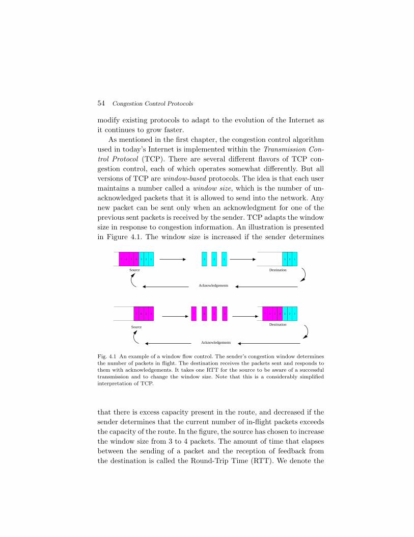
54 Congestion Control Protocols
modify existing protocols to adapt to the evolution of the Internet as
it continues to grow faster.
As mentioned in the first chapter, the congestion control algorithm
used in today’s Internet is implemented within the Transmission Con-
trol Protocol (TCP). There are several different flavors of TCP con-
gestion control, each of which operates somewhat differently. But all
versions of TCP are window-based protocols. The idea is that each user
maintains a number called a window size, which is the number of un-
acknowledged packets that it is allowed to send into the network. Any
new packet can be sent only when an acknowledgment for one of the
previous sent packets is received by the sender. TCP adapts the window
size in response to congestion information. An illustration is presented
in Figure 4.1. The window size is increased if the sender determines
6
123
Destination
Source
Acknowledgements
Acknowledgements
457
Destination
Source
13456
1234567 456
123
7
7 2
Fig. 4.1 An example of a window flow control. The sender’s congestion window determinesthe number of packets in flight. The destination receives the packets sent and responds tothem with acknowledgements. It takes one RTT for the source to be aware of a successful
transmission and to change the window size. Note that this is a considerably simplifiedinterpretation of TCP.
that there is excess capacity present in the route, and decreased if the
sender determines that the current number of in-flight packets exceeds
the capacity of the route. In the figure, the source has chosen to increase
the window size from 3 to 4 packets. The amount of time that elapses
between the sending of a packet and the reception of feedback from
the destination is called the Round-Trip Time (RTT). We denote the
4.1. TCP-Reno 55
RTT by T . A decision on whether to send a new packet, and whether
the window is to be increased or decreased, is taken upon reception
of the acknowledgement packet. This means that the decision-making
process has no periodicity that is decided by a clock of fixed frequency.
TCP is therefore called self-clocking. The nearest approximation to a
clock is the round-trip time T , which could potentially vary during the
lifetime of a flow. The exact means of determining whether to increase
or decrease the window size is what determines the difference between
the congestion control mechanism of different TCP flavors which we
discuss in the rest of this chapter.
4.1 TCP-Reno
The most commonly used TCP flavors used for congestion control in
the Internet today are Reno and NewReno. Both of them are updates of
the TCP-Tahoe, which was introduced in 1988. Although they vary sig-
nificantly in many regards, the basic approach to congestion control is
similar. The idea is to use successful reception packets as an indication
of available capacity and dropped packets as an indication of conges-
tion. We consider a simplified model for the purpose of exposition. Each
time the destination receives a packet, it sends and acknowledgement
(also called ack) asking for the next packet in sequence. For example,
when packet 1 is received, the acknowledgement takes the form of a
request for packet 2. If, instead of the expected packet 2, the desti-
nation receives packet 3, the acknowledgement still requests packet 2.
Reception of three duplicated acknowledgments or dupacks (i.e., four
successive identical acks) is taken as an indication that packet 2 has
been lost due to congestion. The source then proceeds to cut down the
window size and also to re-transmit lost packets. In case the source
does not receive any acknowledgements for a finite time, it assumes
that all its packets have been lost and times out.
When a non-duplicate acknowledgment is received, the protocol in-
creases its window size. The amount by which the window size is in-
creases depends upon the TCP transmission phase. TCP operates in
two distinct phases. When file transfer begins, the window size is 1,
but the source rapidly increases its transmission window size so as to
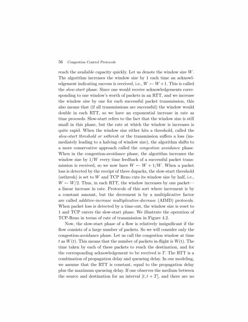
56 Congestion Control Protocols
reach the available capacity quickly. Let us denote the window size W .
The algorithm increases the window size by 1 each time an acknowl-
edgement indicating success is received, i.e., W ←W +1. This is called
the slow-start phase. Since one would receive acknowledgements corre-
sponding to one window’s worth of packets in an RTT, and we increase
the window size by one for each successful packet transmission, this
also means that (if all transmissions are successful) the window would
double in each RTT, so we have an exponential increase in rate as
time proceeds. Slow-start refers to the fact that the window size is still
small in this phase, but the rate at which the window is increases is
quite rapid. When the window size either hits a threshold, called the
slow-start threshold or ssthresh or the transmission suffers a loss (im-
mediately leading to a halving of window size), the algorithm shifts to
a more conservative approach called the congestion avoidance phase.
When in the congestion-avoidance phase, the algorithm increases the
window size by 1/W every time feedback of a successful packet trans-
mission is received, so we now have W ← W + 1/W . When a packet
loss is detected by the receipt of three dupacks, the slow-start threshold
(ssthresh) is set to W and TCP Reno cuts its window size by half, i.e.,
W ←W/2. Thus, in each RTT, the window increases by one packet—
a linear increase in rate. Protocols of this sort where increment is by
a constant amount, but the decrement is by a multiplicative factor
are called additive-increase multiplicative-decrease (AIMD) protocols.
When packet loss is detected by a time-out, the window size is reset to
1 and TCP enters the slow-start phase. We illustrate the operation of
TCP-Reno in terms of rate of transmission in Figure 4.2.
Now, the slow-start phase of a flow is relatively insignificant if the
flow consists of a large number of packets. So we will consider only the
congestion-avoidance phase. Let us call the congestion window at time
t as W (t). This means that the number of packets in-flight is W(t). The
time taken by each of these packets to reach the destination, and for
the corresponding acknowledgement to be received is T. The RTT is a
combination of propagation delay and queueing delay. In our modeling,
we assume that the RTT is constant, equal to the propagation delay
plus the maximum queueing delay. If one observes the medium between
the source and destination for an interval [t, t + T ], and there are no
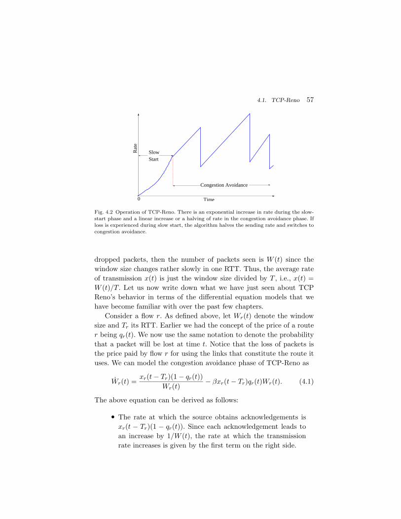
4.1. TCP-Reno 57
Rat
e
Time 0
Congestion Avoidance
SlowStart
Fig. 4.2 Operation of TCP-Reno. There is an exponential increase in rate during the slow-
start phase and a linear increase or a halving of rate in the congestion avoidance phase. Ifloss is experienced during slow start, the algorithm halves the sending rate and switches to
congestion avoidance.
dropped packets, then the number of packets seen is W (t) since the
window size changes rather slowly in one RTT. Thus, the average rate
of transmission x(t) is just the window size divided by T , i.e., x(t) =
W (t)/T. Let us now write down what we have just seen about TCP
Reno’s behavior in terms of the differential equation models that we
have become familiar with over the past few chapters.
Consider a flow r. As defined above, let Wr(t) denote the window
size and Tr its RTT. Earlier we had the concept of the price of a route
r being qr(t). We now use the same notation to denote the probability
that a packet will be lost at time t. Notice that the loss of packets is
the price paid by flow r for using the links that constitute the route it
uses. We can model the congestion avoidance phase of TCP-Reno as
Wr(t) =xr(t− Tr)(1− qr(t))
Wr(t)− βxr(t− Tr)qr(t)Wr(t). (4.1)
The above equation can be derived as follows:
• The rate at which the source obtains acknowledgements is
xr(t − Tr)(1 − qr(t)). Since each acknowledgement leads to
an increase by 1/W (t), the rate at which the transmission
rate increases is given by the first term on the right side.
58 Congestion Control Protocols
• The rate at which packets are lost is xr(t − Tr)qr(t). Such
events would cause the rate of transmission to be decreased
by a factor that we call β. This is the second term on the
right side. Considering the fact that there is a halving of
window size due to loss of packets, β would naturally taken
to be 1/2. However, studies show that a more precise value of
β when making a continuous-time approximation of TCP’s
behavior is close to 2/3.
To compare the TCP formulation above to the resource allocation
framework, we write Wr(t) in terms of xr(t) which yields
xr =xr(t− Tr)(1− qr(t))
T 2r xr
− βxr(t− Tr)qr(t)xr(t). (4.2)
The equilibrium value of xr is found by setting xr = 0, and is seen to
be
xr =
√
1− q
βq
1
Tr,
where qr is the equilibrium loss probability. For small values of qr (which
is what one desires in the Internet),
xr ∝ 1/Tr
√
qr.
This result is well-known and widely used in the performance analysis
of TCP.
4.2 Relationship with Primal Algorithm
Now, consider the controller (4.2) again. Suppose that there were no
feedback delay, but the equation is otherwise unchanged. So T 2r that
appears in (4.2) is just some constant now. Also, let qr(t) be small, i.e.,
the probability of losing a packet is not too large. Then the controller
reduces to
xr =1
T 2r
− βx2rqr
= βx2r
(
1
βT 2r x2
r
− qr
)
.
4.3. A Generalization of TCP-Reno 59
Comparing with (3.5), we find that the utility function of the source r
satisfies
U ′r(xr) =
1
βT 2r x2
r
.
We can find the source utility (up to an additive constant) by integrat-
ing the above, which yields
Ur(xr) = − 1
βT 2r xr
.
Thus, TCP can be approximately viewed as a control algorithm that
attempts to achieve weighted minimum potential delay fairness.
If we do not assume that qr is small, the delay-free differential equa-
tion is given by
xr =1− qr
T 2r
− βx2rqr
= (βx2r + 1/T 2
r )
(
1
βT 2r x2
r + 1− qr
)
,
Thus,
U ′r(xr) =
1
βT 2r x2
r + 1⇒ Ur(xr) =
1
Tr√
βtan−1
(
√
βTr xr
)
,
where the utility function is determined up to an additive constant.
4.3 A Generalization of TCP-Reno
Instead of increasing the window size by 1/W for each ack and de-
creasing the window by 1/2 upon detecting a loss, one could con-
sider other increase-decrease choices as well. Consider a protocol where
W ← W + a Wn when an acknowledgement is received, while a
loss triggers a window decrease given by W ← W − b Wm. Setting
a = 1, n = −1, b = 0.5, and m = 1 would yield TCP-Reno type
behavior. The equivalent rate-based equation describing the dynamics
of such a protocol would be
xr =xr(t− Tr)
Tr(a(xr(t) Tr)
n(1− qr(t)) − b(xr(t) Tr)mqr(t)) . (4.3)
60 Congestion Control Protocols
Ignoring the feedback delay in obtaining the congestion information,
the above differential equation becomes
xr =xr(t)
Tr(a(xr(t) Tr)
n(1− qr(t)) b(xr(t) Tr)mqr(t)) ,
which can be rewritten as
xr = (axr(t)n+1Tn−1
r )
(
1 +b
a(xr(t)Tr)
m−n
)
(
1
1 + ba(xr(t)Tr)m−n
− qr
)
.
Note that1
1 + ba(xr(t)Tr)m−n
is a decreasing function (thus, its derivative will be negative) if m > n
and hence one can view the above differential equation as the congestion
controller for a source r with a concave utility function
∫ xr(t)
0
1
1 + ba(xTr)m−n
dx.
A special case of the above congestion control algorithm called Scalable-
TCP which uses the parameters a = 0.01, n = 0, b = 0.125, and m = 1
has been proposed for high-bandwidth environments.
4.4 TCP-Vegas: A Delay Based Algorithm
We now consider another variation of TCP called TCP-Vegas. TCP-
Vegas uses queueing delay to infer congestion in the network. The idea
is to first identify the propagation delay of the route by assuming that
it is equal to the smallest RTT seen by the source. This is a reasonable
assumption if we assume that queues empty occasionally in which case
the only delay is the propagation delay. Let us denote the estimated
propagation delay by Tp. Any excess delay above this amount would
be queueing delay and we denote it Tq. The objective of the algorithm
is to calculate the value of window size such that there is no queueing
delay. When this occurs, the rate of generation of packets is equal to
the available capacity on the route. We now study the details of this
algorithm.
4.4. TCP-Vegas: A Delay Based Algorithm 61
If there is no queueing delay, the throughput would be approxi-
mately given by
e =W
Tp,
where W is the window size. However, the actual throughput is the
number of packets that make it successfully to the destination in a
fixed amount of time. To calculate this quantity, the source sends a
marked packet and waits for it to be acknowledged. The duration of
time that it takes for this event to occur is the round-trip time Tp +Tq.
Suppose during this time, the source receives S acknowledgments, then
the actual throughput is estimated as
a =S
Tp + Tq.
Whenever we receive the acknowledgment for a marked packet at
some time t, we have two values—the expected throughput e(t) and
the actual throughput a(t). If a(t) is less than e(t), it means that our
transmission rate is too high, so we should cut down the window size.
On the other hand, if a(t) is greater than e(t), it means that the esti-
mate of the available rate is too low and we should increase the window
size. Formally, we define constants α and β, with α ≤ β and proceed
as follows:
• if α ≤ (e(t)−a(t)) ≤ β, then do nothing. This means that our
estimate of the throughput is fairly accurate, and everything
is as it should be.• if (e(t) − a(t)) > β, decrease the window size by 1 for the
next RTT. This means that our estimate is too high and the
window size must be reduced.• if (e(t) − a(t)) < α, increase the window size by 1 for the
next RTT. This means that our estimate is too low and the
network can support more than we think.
Note that both the increase and decrease of window size are linear in
nature. Also, the algorithm uses the usual slow start mechanism, with
exponential growth initially. The behavior of TCP-Vegas under ideal
conditions would look something like Figure 4.3.
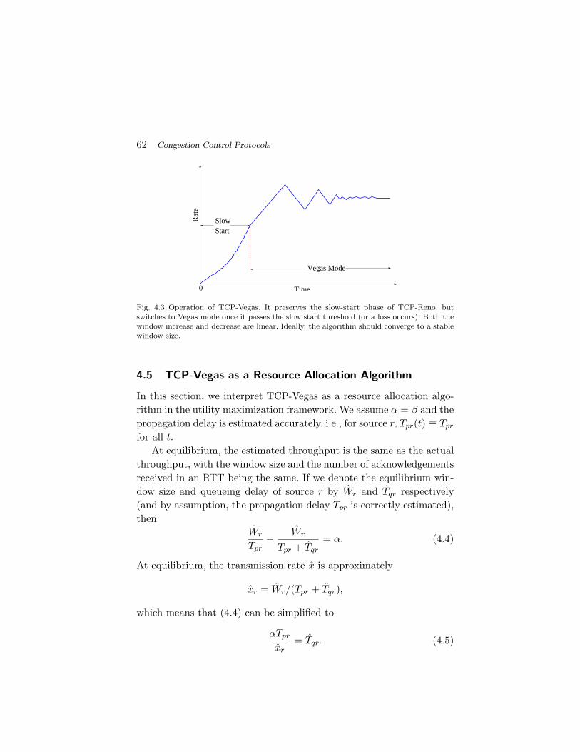
62 Congestion Control Protocols
Time 0
SlowStart
Rat
e
Vegas Mode
Fig. 4.3 Operation of TCP-Vegas. It preserves the slow-start phase of TCP-Reno, but
switches to Vegas mode once it passes the slow start threshold (or a loss occurs). Both thewindow increase and decrease are linear. Ideally, the algorithm should converge to a stable
window size.
4.5 TCP-Vegas as a Resource Allocation Algorithm
In this section, we interpret TCP-Vegas as a resource allocation algo-
rithm in the utility maximization framework. We assume α = β and the
propagation delay is estimated accurately, i.e., for source r, Tpr(t) ≡ Tpr
for all t.
At equilibrium, the estimated throughput is the same as the actual
throughput, with the window size and the number of acknowledgements
received in an RTT being the same. If we denote the equilibrium win-
dow size and queueing delay of source r by Wr and Tqr respectively
(and by assumption, the propagation delay Tpr is correctly estimated),
then
Wr
Tpr− Wr
Tpr + Tqr
= α. (4.4)
At equilibrium, the transmission rate x is approximately
xr = Wr/(Tpr + Tqr),
which means that (4.4) can be simplified to
αTpr
xr= Tqr. (4.5)
4.5. TCP-Vegas as a Resource Allocation Algorithm 63
Now that we know what the equilibrium transmission rate looks like,
let us study what the equilibrium queueing delay Tqr would look like. If
the queue length at equilibrium is denoted by bl, then the equilibrium
queueing delay at link l is bl/cl (where cl is the capacity of link l). So
we have
Tqr =∑
l:l∈r
bl
cl. (4.6)
Also, if∑
k:l∈k
xk < cl,
then there is no queueing delay, i.e., bl = 0 in this case. Note that
since the aggregate equilibrium transmission rate of all flows using link
l cannot exceed the link capacity, we cannot possibly have that∑
k:l∈k
xk > cl.
Thus, if bl 6= 0, it means that∑
k:l∈k
xk = cl.
Thus, we have from the above and (4.5), that the equilibrium con-
ditions areαTpr
xr=∑
l:l∈r
bl
cl,
withbl
cl
(
∑
k:l∈k
xk − cl
)
= 0 ∀ l.
However, these are the Karush-Kuhn-Tucker conditions for the util-
ity maximization problem
max{xr}
αTpr log xr, (4.7)
subject to∑
r:l∈r
xr ≤ cl, ∀ l
64 Congestion Control Protocols
and xr ≥ 0, ∀r. Thus, TCP-Vegas is weighted-proportionally fair. If we
let each flow have a different value of α, i.e., we associate αr with route
r, , then the equilibrium rates will maximize∑
r αrTpr log xr.
4.6 Relation to Dual Algorithms and Extensions
We now consider the relationship between TCP-Vegas and dual algo-
rithms. A weighted proportionally fair dual algorithm would use the
controller obtained by substituting wr log(xr) as the utility function in
(3.23) and (3.24), which yields
xr =wr
prand (4.8)
pl = hl(yl − cl)+pl
, (4.9)
To avoid confusion, we note that wr is the weight assigned to source r
and is unrelated to the window size Wr(t). If we choose hl = 1cl
, then
the price function of a link becomes the queueing delay experienced by
packets using that link, which, when added to a constant propagation
delay, is the feedback that is used in the Vegas algorithm.
Let us study the source rates used in Vegas more closely to create
a fluid model equivalent. From the algorithm description (with α = β)
we have that the Vegas algorithm updates the window Wr(t) based on
whether
Wr(t)
Tpr− Wr(t)
Tpr + Tqr(t)< α or
Wr(t)
Tpr− Wr(t)
Tpr + Tqr(t)> α, (4.10)
Using the approximation xr(t) = Wr(t)Tpr+Tqr(t) , we can rewrite the condi-
tions as
xr(t) Tqr(t) < αTpr or xr(t) Tqr(t) > αTpr. (4.11)
As in (4.6), we also have
Tqr =∑
l:l∈r
bl(t)
cl=∑
l:l∈r
pl(t), (4.12)
where bl(t) is the queue length at link l at time t, and we have used
pl(t) to denote the queueing delay at link l, which acts as the price
4.6. Relation to Dual Algorithms and Extensions 65
function for Vegas. Combining the above expressions, the condition for
increase/decrease becomes
xr(t)∑
l:l∈r
pl(t) < αTpr or xr(t)∑
l:l∈r
pl(t) > αTpr, (4.13)
So the window control algorithm can be written as
Wr(t + 1) =
[
Wr(t) +1
Tpr + Tqr(t)sgn (αTpr − xr(t) Tqr)
]+
Wr
, (4.14)
where sgn(z)= −1 if z < 0 and sgn(z)= 1 if z > 0. Thus, we can
now write down the differential equations describing the TCP-Vegas
algorithm as
pl(t) =1
cl(yl − cl)
+pl
(4.15)
Wr(t) =
[
1
Tpr + Tqr(t)sgn (αTpr − xr(t) Tqr(t))
]+
Wr
(4.16)
xr(t) =Wr(t)
Tpr + Tqr(t), (4.17)
with Tqr(t) =∑
l:l∈r pl(t). The above is not the same as the dual al-
gorithm that we derived in the previous chapter. However, the price
update dynamics are the same as the price update for the dual algo-
rithm. Further, at the source, by attempting to increase or decrease
the rate based on whether xr is less than or greater than αTpr/Tqr, it
is clear the source attempts to drive the system towards
xr =αTpr
Tqr=
αTpr∑
l∈r pl,
which is the desired source behavior for a dual congestion controller.
Thus, one can interpret TCP-Vegas as an algorithm that approximates
the dual congestion control algorithm.
A modification of TCP-Vegas called FAST-TCP has been suggested
for very high-speed networks. In FAST-TCP, the window size is in-
creased or decreased depending upon how far the window size is from
66 Congestion Control Protocols
a desired equilibrium point. The fluid model describing the protocol is
pl(t) =1
cl(yl − cl)
+pl
(4.18)
Wr(t) = γr (αr − xr(t) Tqr)+Wr
(4.19)
xr(t) =Wr(t)
Tpr + Tqr(t), (4.20)
where αr determines the desired equilibrium point and γr is a scaling
constant. Replacing the sgn function in TCP-Vegas with the difference
between the current operating point and the desired equilibrium allows
FAST-TCP to rapidly approach the desired equilibrium point.
4.7 Notes
In this chapter we studied how Internet congestion control protocols can
be viewed as decentralized resource allocation algorithms. TCP-Reno,
NewReno and SACK are improvements on TCP-Tahoe proposed by
Jacobson [1]. Details of the protocols studied are available in [49–51].
The differential equation for TCP without time delays was introduced
by Kunniyur and Srikant in [31, 52] who also noted the connection to
minimum potential delay fairness while a delay differential equation
model was introduced by Misra et. al. in [53]. The choice of the arctan
utility function for TCP was proposed by Kelly [9]. The differential
equations models are approximations of stochastic, discrete models and
the regimes under which a differential equation approximation hold
have been explored in Baccelli et. al. [54], Shakkottai and Srikant [55,56]
and Tinnakornsrisuphap and Makowski [57]. The model for Scalable
TCP was proposed by Vinnicombe [58] and implemented by Tom Kelly
[59]. TCP-Vegas was proposed by Bramko and Peterson in [60], while
the analytical study was presented by Low et. al in [61]. A comparison
of the throughput that TCP-Vegas and TCP-Reno sources achieve in a
network may be found in [62] by Mo et. al. A description of how Vegas
was modified to create FAST-TCP was presented by Wei et. al. in [63],
and implementation details of FAST TCP are provided in [64]. The fluid
models for TCP capture the behavior of TCP reasonably well in large
networks with a large number of users. However, in some instances,
one needs more detailed modeling of the window size evolution of TCP.
4.7. Notes 67
Models to capture the window size behavior in more detail can be found
in the works of Baccelli and Hong [65], Wirth et al [66] and Kherani
et al. [67]. Some of these models present properties of TCP resource
sharing that are not always observable using the coarser differential
equation models. Examples of protocols that are designed using these
finer models are H-TCP [68] and TCP-Illinois [69].
One aspect of resource allocation algorithms that we have not con-
sidered so far is the impact of feedback delay on their convergence.
Another aspect to be considered while studying real-life networks is
the fact that the flows are not persistent. In fact, a user arrives with a
file to be transferred over the network and departs when the file trans-
fer is complete. We have not yet considered the question of whether
the system would be stable in such a scenario. In the next chapter, we
expand our models to incorporate delays and file arrivals and depar-
tures.

5
Network Stability
In the previous chapters, we have studied networks with a fixed number
of flows and assumed that packets traverse from one node to the next
instantaneously. An exception was our discussion on TCP modeling,
where we explicitly incorporated delay in the model. However, we did
not discuss the impact of delay on network stability. In this chapter,
we will explicitly consider the impact of delays and flow arrivals and
departures on network stability. The two effects that we will study are
shown in Figure 5.1. We motivate the two stability issues below, and
consider their impact on network stability in the sections to follow.
In most of the models used in the previous chapters, flows receive
feedback instantaneously. However, in real life there is always a delay
between sending a packet and receiving the corresponding acknowledg-
ment. We call this the Round Trip Time (RTT). The delay consists of
both queueing and propagation delays. For example, the coast-to-coast
distance of the United States is about 5000 kilometers. Since the speed
of light in optical fiber is 1.5 × 10⁸ m/s, the round trip propagation
delay is about 60 msecs. Propagation delays can get even larger when
packets have to traverse the globe. The queueing delay is a function
of the load on the system, and with good design can be kept within
69
70 Network Stability
Departures
Departures
In Progress
In P
rogr
ess
Des
tinat
ions
Feedback
Link
Feedback
Arriva
ls
Arrivals
Fig. 5.1 Two separate phenomena in a network. Flows in progress compete with each other
for bandwidth and keep the link filled. If their transfer rates converge, we say that the systemis stable at a small time scale. Flows arrive bringing a file of fixed size to be transferred
and leave when the transfer is complete. We say that the system is stable at a large timescale if the number of flows in progress is finite at all times.
limits. The RTT is considerably larger than the amount of time that
it takes for a high-speed router to process a packet. For example, the
size of an Internet packet is approximately 10, 000 bits and when it
goes through a 1 Gbps router, the processing time is 105/109 secs. or
0.1 msecs. Thus, one has to worry about the impact of a source react-
ing to congestion that happened some time ago. In particular, one has
to make sure that the system parameters are designed to ensure the
stability of a system of delay-differential equations.
Another effect that we need to include in our model is the fact that
the flows in the system do not stay forever. Flows arrive with a file to be
transferred, and leave once the transfer is complete. So if, on average,
there were 2 flows arriving per second, each with a file transfer of size 10
MB, then the average load on the system would be 160 Mbps. If there
is only one link in the network and the link’s capacity is larger than 160
Mbps, then most reasonable resource allocation algorithms will ensure
that the number of files in the network is bounded in some appropriate
5.1. Stability of the Primal Algorithm with Delays 71
stochastic sense. On the other hand, if the network comprises of many
links and different flows have different sets of links on their route, then
the interaction among the flows could be complex and the allocation of
resources in one part of the network would have an impact on flows in
another part of the network. In this case, the stability of the network is
not obvious even if the total load on each link is less than its capacity.
We will show that, under reasonable assumptions, the network is stable
if one uses the optimization approach to resource allocation.
We note that there are two forms of stability that we consider in
this chapter and these are quite different:
(1) We first consider a fixed number of flows which exercise con-
gestion control, but where the congestion feedback is ob-
tained by the sources with some delay. In this case, we say
that the system is stable if the set of arrival rates converges
to the solution of the network utility maximization problem.
(2) Next, we consider flow arrivals and departures and assume
that the network uses the network utility maximization
framework to allocate the resources. In this case, we say that
the system is stable if the number of flows in the network
stays bounded when the traffic load on each link is less than
its capacity.
Let us first study the stability of the resource allocation algorithm
in the presence of feedback delays.
5.1 Stability of the Primal Algorithm with Delays
We consider the primal algorithm with multi-path routing as we did in
Section 3.3. We recall the notation introduced earlier for the reader’s
convenience. As before, let the set of links be L and the set of sources
be S. Each source s ∈ S identifies a unique source-destination pair.
Also, each source has a collection of routes that it may use. If source
s transmits on route r, we say r ∈ s. Similarly, if a route r uses link
j, we say j ∈ r. For each route r we let s(r) be the unique source
such that r ∈ s(r). We call the set of routes R. Note that two paths
in the network that are otherwise identical can be associated with two
72 Network Stability
different indices r ∈ R, if their sources are different, i.e., two sources
that have the same origin and destination would have different indices
for their routes, even if the physical paths they use are the same.
Source Destination
j
T
T
jr
rj
Fig. 5.2 The RTT is composed of two elements—the delay for a packet to get to an inter-
mediate link, and the delay for feedback from that link back to the source.
In what follows, we will assume that queueing delays are negligible.
We can also think of the queueing delays as constant, i.e., the sum of
queueing and propagation delay is counted as the feedback delay. While
it can be argued that the queueing delay is not constant with time, if
we ensure that it remains bounded, we can take the maximum delay
as the worst-case situation that the controller faces. This is only an
approximation but it provides good qualitative insight into the design
of congestion control algorithms. We let Trj be the amount of time
that it takes for a packet from source r to reach link j. We denote the
feedback delay from link j to source r by Tjr. An illustration of these
two delays is provided in Figure 5.2. The sum Trj + Tjr = Tr, which is
the RTT of the route r. Note that Tr = Trj + Tjr ∀j.The problem of deriving conditions for global asymptotic stability
for this scenario is not straightforward and, at the time of writing
this monograph, is still an open problem. We will linearize the system
around its equilibrium point and obtain conditions for local asymptotic
stability. Simulations suggest that the linearized stability conditions
serve as good guidelines for designing stable congestion controllers.
Once we linearize a system, we can bring into force tools from linear
control theory in order to analyze it. In particular, we can use Laplace
transforms and study the system in the complex domain. We will make
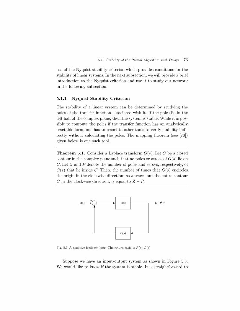
5.1. Stability of the Primal Algorithm with Delays 73
use of the Nyquist stability criterion which provides conditions for the
stability of linear systems. In the next subsection, we will provide a brief
introduction to the Nyquist criterion and use it to study our network
in the following subsection.
5.1.1 Nyquist Stability Criterion
The stability of a linear system can be determined by studying the
poles of the transfer function associated with it. If the poles lie in the
left half of the complex plane, then the system is stable. While it is pos-
sible to compute the poles if the transfer function has an analytically
tractable form, one has to resort to other tools to verify stability indi-
rectly without calculating the poles. The mapping theorem (see [70])
given below is one such tool.
Theorem 5.1. Consider a Laplace transform G(s). Let C be a closed
contour in the complex plane such that no poles or zeroes of G(s) lie on
C. Let Z and P denote the number of poles and zeroes, respectively, of
G(s) that lie inside C. Then, the number of times that G(s) encircles
the origin in the clockwise direction, as s traces out the entire contour
C in the clockwise direction, is equal to Z − P.
+P(s)
Q(s)
x(s) y(s)
−
Fig. 5.3 A negative feedback loop. The return ratio is P (s) Q(s).
Suppose we have an input-output system as shown in Figure 5.3.
We would like to know if the system is stable. It is straightforward to
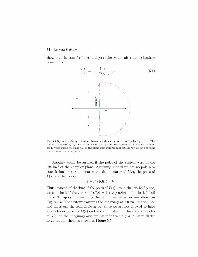
74 Network Stability
show that the transfer function L(s) of the system after taking Laplace
transforms is
y(s)
x(s)=
P (s)
1 + P (s) Q(s). (5.1)
x
Real
Imag
inar
y
x
Fig. 5.4 Nyquist stability criterion. Zeroes are shown by an ’o’ and poles by an ’x’. The
zeroes of 1 + P (s) Q(s) must lie in the left half plane. Also shown is the Nyquist contourused, which spans the right half of the plane with infinitesimal detours to take into accountthe zeroes on the imaginary axis.
Stability would be assured if the poles of the system were in the
left half of the complex plane. Assuming that there are no pole-zero
cancelations in the numerator and denominator of L(s), the poles of
L(s) are the roots of
1 + P (s)Q(s) = 0.
Thus, instead of checking if the poles of L(s) lies in the left-half plane,
we can check if the zeroes of G(s) = 1 + P (s)Q(s) lie in the left-half
plane. To apply the mapping theorem, consider a contour shown in
Figure 5.5. The contour traverses the imaginary axis from −i∞ to +i∞and maps out the semi-circle at ∞. Since we are not allowed to have
any poles or zeroes of G(s) on the contour itself, if there are any poles
of G(s) on the imaginary axis, we use infinitesimally small semi-circles
to go around them as shown in Figure 5.5.
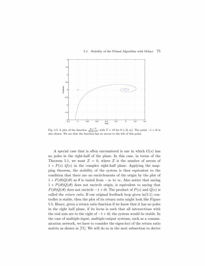
5.1. Stability of the Primal Algorithm with Delays 75
−1.2 −1 −0.8 −0.6 −0.4 −0.2 0 0.2 0.4−2
−1.5
−1
−0.5
0
0.5
1
1.5
2
Real
Imag
inar
y
Fig. 5.5 A plot of the function Te−iθ
iθ(iθ+T )with T = 10 for θ ∈ [0,∞]. The point −1 + i0 is
also shown. We see that the function has no zeroes to the left of this point.
A special case that is often encountered is one in which G(s) has
no poles in the right-half of the plane. In this case, in terms of the
Theorem 5.1, we want Z = 0, where Z is the number of zeroes of
1 + P (s) Q(s) in the complex right-half plane. Applying the map-
ping theorem, the stability of the system is then equivalent to the
condition that there are no encirclements of the origin by the plot of
1 + P (iθ)Q(iθ) as θ is varied from −∞ to ∞. Also notice that saying
1 + P (iθ)Q(iθ) does not encircle origin, is equivalent to saying that
P (iθ)Q(iθ) does not encircle −1 + i0. The product of P (s) and Q(s) is
called the return ratio. If our original feedback loop given in(5.1) con-
troller is stable, then the plot of its return ratio might look like Figure
5.5. Hence, given a return ratio function if we know that it has no poles
in the right half plane, if its locus is such that all intersections with
the real axis are to the right of −1+ i0, the system would be stable. In
the case of multiple-input, multiple-output systems, such as a commu-
nication network, we have to consider the eigen-loci of the return ratio
matrix as shown in [71]. We will do so in the next subsection to derive
76 Network Stability
linear stability conditions for the primal congestion control algorithms.
The application of the mapping theorem to test for the stability of a
linear system is called the Nyquist criterion.
5.1.2 Network Stability
We now have the tools required to tackle the question of multi-path
linearized stability. The controller that we use in this section is as
follows:
d
dtxr(t) = κrxr(t)
(
1− qr(t)
U ′s(r)(zs(r)(t))
)+
xr(t)
(5.2)
where
qr(t) =∑
j∈r
pj(t− Tr) (5.3)
and
pj(t) = fj(yj(t)), yj(t) =∑
r:j∈r
xr(t− Tr) (5.4)
and
zs(t) =∑
r∈s
xr(t− Tr) (5.5)
The controller is slightly different from the one we saw in Section 3.3.
In the absence of delay, it is easy to see that it is a gradient algorithm
to maximize the following objective:
U(x) =∑
s
wsUs
(
∑
r∈s
xr
)
−∑
l
∫
P
k:l∈k xk
0fl(y) dy. (5.6)
Even if Us(.) is strictly concave and fl is a non-decreasing function,
the above objective function need not be strictly concave in x. Thus, it
may not have a unique maximum. On the other hand, the formulation
in Section 3.3 would ensure strict concavity, but the resulting stability
conditions are more complicated. So we assume the formulation in (5.6)
but assume that the maximum is unique. We also assume that the
optimal rates are non-zero along all paths.
5.1. Stability of the Primal Algorithm with Delays 77
Notice that (5.5) implies that the source must keep the rates it
used one RTT ago in its memory. This can be easily implemented by
putting the current rate in the header of each packet and echoing this
rate back in the acknowledgments. Thus, by reading off the rate in the
ack, a source knows that rate that it used on a particular path one
RTT ago.
To motivate the stability result, consider a differential equation
dx
dt= f(x),
and assume that it is stable. Now, consider a delay-differential equation
dz
dt= κf(z(t− T )).
Rescale time as τ = Kt and define y(τ) = z(τ/K). Straightforward
differentiation using the fact that
dy(τ)
dτ=
dz(t)
dt
dt
dτ
yields the following delay-differential equation for y in the τ timescale:
dy
dτ= f(y(τ − κT )).
If κT = 0, then this is the same as the differential equation for x.
Thus, it seems reasonable to expect the delay-differential equation to
be stable if κT is small. We will show that one can indeed derive such
a stability condition for the network. Specifically, it will be shown that
the following conditions are sufficient for linear stability:
κrTr
qr
−U ′′s(r)zs(r) +
∑
j∈r
yj f′j
<π
2, (5.7)
where we have used the notation ˆ to indicate equilibrium points.
We will prove the result by first linearizing the controller around its
equilibrium, taking Laplace transforms and studying the spectrum of
the return ratio in the complex domain using the Nyquist condition.
The equilibrium condition of the controller is given by
U ′s(r)
(
∑
r:r∈s
xr
)
=∑
fj
∑
a:j∈a
xa
(5.8)
78 Network Stability
for each r. Let xr(t) = xr + ur(t), zs(t) = zs + vs(t), and yj(t) =
yj +wj(t). Then linearizing the controller about the equilibrium yields
d
dtur(t) = −κrxr
qr
−U ′′s(r)vs(t)(t) +
∑
j∈r
f ′jwj(t− Tjr)
, (5.9)
vs(t) =∑
r:r∈s
ur(t− Tr), (5.10)
wj(t) =∑
r:j∈r
ur(t− Tj). (5.11)
We now proceed to take Laplace transforms of the above linear
system. The fact that we are now working in the complex domain
is shown by t being replaced by s for all the variables. We use s to
represent the Laplace domain variable to avoid any confusion with the
source variable s.
sur(s) = −κrxr
qr
−U ′′s(r)vs(s) +
∑
j∈r
f ′je
−sTjrwj(s)
, (5.12)
vs(s) =∑
r:r∈s
e−sTrur(s), (5.13)
wj(s) =∑
r:j∈r
e−sTrjur(s). (5.14)
The above equations can be compactly written as(
v(s)
w(s)
)
= F−1R(−s)T X(s)R(s)F
(
v(s)
w(s)
)
, (5.15)
where X(w) is an |R| × |R| diagonal matrix, with entries Xrr(s) =
e−sTr/sTr and F is a |S|+ |L|× |S|+ |L| diagonal matrix whose entries
are Fss = 1, Fjj = (f ′j)
12 , and R(s) is a |R| × (|S|+ |L|) matrix with
Rrs(s) =
(
−U ′′s(r)Tr
κrxr
qr
) 12
, r ∈ s
Rrj(s) = e−sTjr
(
κrxr
qrTrf
′j
) 12
, j ∈ r
and all other entries are 0.
5.1. Stability of the Primal Algorithm with Delays 79
The matrix F−1R(−s)T X(s)R(s)F that appears in (5.15) is the
return ratio of the controller, and we would like to study the eigenvalues
of this matrix to see if they lie to the right of −1 + i0. Let λ be an
eigenvalue of the above matrix. Then we have
λy = R(iθ)⋆ X(iθ) R(iθ) y,
where ⋆ is used to indicate the matrix conjugate transpose. Thus we
have
λ = y⋆ R(iθ)⋆ X(iθ) R(iθ) y.
If d = R(iθ)y, then since X is a diagonal matrix
λ =∑
r
|dr|2Xrr(iθ) =∑
r
|dr|2e−iθTr
iθTr.
So we can write λ = Kζ, where K = ||R(iθ)y||2 and ζ lies in the convex
hull of{
e−iθTr
iθTr: r ∈ s, s ∈ S
}
.
Now, as shown in Figure 5.6, the convex hull includes the point −2/π
on its boundary, but has no point to the left of this on the real axis.
This means that if λ is real, then λ ≥ (−2/π)K.
It remains now to find a bound on K. Let P be the |S|+|L|×|S|+|L|diagonal matrix taking the values Pss = zs
√
−U ′′ and Pjj = yj
√
f ′j .
We let ρ(.) denote the spectral radius and ||.||∞ the maximum row sum
matrix norm. So we now have
K = y⋆R(iθ)⋆R(iθ)y
≤ ρ(R(iθ)⋆R(iθ))
= ρ(P−1 R(iθ)⋆R(iθ) P )
≤ ||P−1 R(iθ)⋆R(iθ) P ||∞<
π
2,
where the last inequality follows form our choice made in (5.7). This
means that any real eigenvalue λ must lie to the right of −1 and the
Nyquist condition, as outlined earlier is satisfied. Thus, the multi-path
controller is stable around its equilibrium point with our choice of κr.
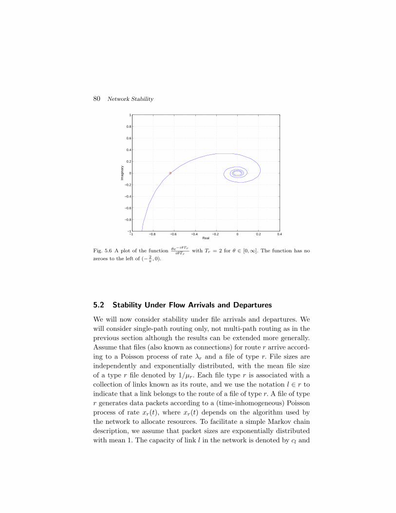
80 Network Stability
−1 −0.8 −0.6 −0.4 −0.2 0 0.2 0.4−1
−0.8
−0.6
−0.4
−0.2
0
0.2
0.4
0.6
0.8
1
Real
Imag
inar
y
Fig. 5.6 A plot of the function θe−iθTr
iθTrwith Tr = 2 for θ ∈ [0,∞]. The function has no
zeroes to the left of (− 2π
, 0).
5.2 Stability Under Flow Arrivals and Departures
We will now consider stability under file arrivals and departures. We
will consider single-path routing only, not multi-path routing as in the
previous section although the results can be extended more generally.
Assume that files (also known as connections) for route r arrive accord-
ing to a Poisson process of rate λr and a file of type r. File sizes are
independently and exponentially distributed, with the mean file size
of a type r file denoted by 1/µr. Each file type r is associated with a
collection of links known as its route, and we use the notation l ∈ r to
indicate that a link belongs to the route of a file of type r. A file of type
r generates data packets according to a (time-inhomogeneous) Poisson
process of rate xr(t), where xr(t) depends on the algorithm used by
the network to allocate resources. To facilitate a simple Markov chain
description, we assume that packet sizes are exponentially distributed
with mean 1. The capacity of link l in the network is denoted by cl and
5.2. Stability Under Flow Arrivals and Departures 81
we assume the following stability condition:
∑
r:l∈r
λr
µr< cl, ∀l, (5.16)
i.e., we assume that the load on each link is less than the link capac-
ity. The goal is to show that the number of files in the network stays
bounded. The reason for providing the reader with a stochastic descrip-
tion of the system is to let the reader know the model for which the
results of this section applies. However, in keeping with the spirit of
the rest of this monograph, we ignore the stochastic dynamics of the
system and consider a heuristic deterministic differential equation de-
scription of the system and use a Lyapunov function method to show
the boundedness of this system. In the next section, we will refer the
interested reader to papers that provide the details of the proof of
stochastic stability.
At each time instant t, there are nr users on route r. We assume that
all users in the network use the α-fair utility function, with possibility
different weights for different routes, i.e.,
Ur(xr) = wrx1−α
1− α.
At each time instant, the network attempts to solve the utility max-
imization problem using the dual algorithm described in Section 3.2.
Accordingly, the transmission rate xr of a type r source, satisfies
wr
xαr
= qr,
where qr is price of route r and is given by
qr =∑
l:l∈r
pl.
To ensure boundedness of xr when qr = 0, we modify the rate-update
equation as
xr = max{(wr
qr)1/α, M},
where M is some large constant. The price pl is computed using
pl = (yl − cl)+pl
, (5.17)
82 Network Stability
where the arrival rate at each link is given by
yl =∑
s:l∈s
nsxs.
Now, we describe the dynamics of the number of files in the network.
Files on route r arrive at rate r. Since the average file size is 1/µr and
xr is the total rate assigned to a user on route r, the instantaneous rate
at which a file is processed is xrµr. Since there are nr files on route r,
the total rate at which they are processed is µrnrxr. Thus, we get the
following differential equation for nr(t) :
nr = λr − µrnrxr. (5.18)
Consider the Lyapunov function
V (n, p) =1
1 + α
∑
r
K1rn1+αr +
1
2
∑
l
K2lp2l ,
where the constants K1r and K2l will be chosen later. Note that
dV
dt=∑
r
K1rnαr (λr − µrnrxr) +
∑
l
K2lpl(yl − cl),
where we have used the fact pl(yl−cl) = pl(yl−cl)+pl
. From the stability
condition, there exists an ǫ > 0 such that
νl(1 + ǫ) ≤ cl,
where
νl =∑
s:l∈s
ρs, ρs =λs
µs.
5.2. Stability Under Flow Arrivals and Departures 83
Choose such an ǫ, define δ = ǫ/2 and rewrite V as follows:
V = −δ∑
r
K1rnαr λr +
∑
r
K1rnαr µr (ρr(1 + δ)− nrxr)
+∑
l
K2lpl(yl − cl)
= −δ∑
r
K1rnαr λr
+∑
r
K1rµrnr(ρr(1 + δ))α
(
1
(ρr(1 + δ)/nr)α− 1
xαr
)
×(
ρr(1 + δ)
nr− xr
)
Inr>0
+∑
r
K1rµrnr(ρr(1 + δ))α
xαr
(
ρr(1 + δ)
nr− xr
)
Inr>0
+∑
l
K2lpl(yl − cl)
≤ −δ∑
r
K1rnαr λr +
∑
r
K1rµr(ρr(1 + δ))αqr
wr(ρr(1 + δ)− nrxr)
+∑
l
K2lpl(yl − cl) +∑
r
K1rµr(ρr(1 + δ))α
Mαρr(1 + δ),
where the last inequality follows from the fact that 1/xαr is a decreasing
function and qr = wr/xαr if qr 6= 0 and xr = M if qr = 0. Now, choose
K2l = 1 and K1rµr(ρr(1 + δ))α/wr = 1. Then,
V ≤ −δ∑
r
K1rnαr λr +
∑
r
qr(ρr(1 + δ)− nrxr) +∑
l
pl(yl − cl) + K3,
where K3 =∑
r K1rµr(ρr(1+δ))α
Mα ρr(1 + δ). Noting that∑
r
qrρr =∑
l
plνl and∑
r
qrnrxr =∑
l
plyl,
we have
V ≤ −δ∑
r
K1rnαr λr − δ
∑
l
plνl + K3.
From the above equation, it is clear that we can find a bounded set B
such that if (n, p) ∈ B, V (t) decreases. Thus, (n, p) will be ultimately
84 Network Stability
bounded. One can translate this conclusion into an appropriate notion
of stochastic boundedness.
5.3 Notes
Linear stability results for the primal controller were obtained by Vin-
nicombe [58,72], for the dual controller by Paganini et. al. [73], and for
the primal-dual-type controllers by Kunniyur and Srikant [74] and by
Liu et. al. [75]. Stability conditions for the primal multi-path controller
were obtained by Han et. al. in [28] and by Kelly and Voice in [76]. The
results in this chapter follow the derivation by Kelly and Voice. Global
stability results for congestion controllers are available only for certain
limited scenarios and are not treated in this chapter. For the interested
readers, we provide some references here. Conditions for single-link sta-
bility were derived by Hollot and Chait for TCP-type controllers [77],
by Deb and Srikant for proportionally-fair primal controllers [78], and
by Wang and Paganini for dual controllers [79]. Global stability for a
network of primal controllers were derived by Ying et. al. in [80–82]
and for dual controllers by Papachristodoulou [83]. Independent of the
utility maximization framework, stability results for delay-differential
equation models of TCP and AQM schemes were obtained by Misra
et. al. [53], Hollot et. al. [84] and Kunniyur and Srikant [85].
The flow-level model for congestion controllers for a fixed num-
ber of sources, but where the sources alternate between ON and OFF
states were introduced by Heyman et. al. [86]. A single link version of
the model considered in this chapter, but where the congestion con-
trol is assumed to operate instantaneously was considered by Das and
Srikant [87]. The general network assuming congestion control operates
instantaneously compared to the time-scale of file arrivals and depar-
tures was introduced by Roberts and Massoulie in [88]. The stability of
this network was proved by de Veciana et. al. in [89] for max-min con-
gestion controllers and by Bonald and Massoulie in [90]. A stochastic
version of the stability proof of [90] is presented in [91] using an exten-
sion of Lyapunov’s theorem for Markov chains (see [92], for example).
The stability of a model without the time-scale separation between flow
dynamics and congestion control dynamics was shown by Lin, Shroff
5.3. Notes 85
and Srikant [93–95]. All of these results assume that the file sizes are
exponentially distributed. This assumption has been relaxed by Mas-
soulie [96] and Bramson [97] for proportionally-fair and max-min con-
trollers under the time-scale separation. For general α-fair controllers,
partial stability results for a fraction of the possible capacity region
have been reported by Chiang et. al. [98].
We now move away from the question of network stability and
present a different take on network utility maximization. In the next
chapter, we consider a network of rational, selfish users who are capable
of modifying their protocols to some extent, and study their impact on
system performance.

6
Game Theory and Resource Allocation
In this chapter, we consider an alternative interpretation of the utility
maximization problem that we considered earlier in Chapters 2 and 3.
Consider a network planner who is interested in allocating resources to
users with the goal of maximizing the sum of the user’s utilities. The
network planner can do this only if he knows the utility functions of all
the users in the network, or if there is an incentive for the users to reveal
their utility functions truthfully. In this chapter, we will first discuss
an incentive mechanism called the Vickrey-Clarke-Groves (VCG) which
makes it profitable for the users to reveal their true utilities to the cen-
tral network planner. However, the amount of information that needs
to be conveyed by the users and the amount of computation required
on the part of the network planner make it difficult to implement the
VCG mechanism. One can design a mechanism based on the resource
allocation algorithms in Chapters 2 and 3 under which truth-telling is
optimal. We call this the Kelly mechanism. However, this mechanism
is truth-revealing only under the assumption that the network is very
large so that it is difficult for each user to estimate its impact on the
price decided by the network. Users that are unaware of their effect on
the price are called price taking. On the other hand, in a small network
87
88 Game Theory and Resource Allocation
such as a single link, a user may be able to assess its impact on the
network price. In such a case, the user may act strategically, i.e., act in
such a manner that influences the price to maximize its own benefit.
We will review recent results that show that, the inefficiency of the
Kelly mechanism with strategic users is bounded by 25%, i.e.,the Kelly
mechanism loses at the most a factor of 1/4 compared the maximum
possible network utility.
6.1 VCG Mechanism
Consider the problem of dividing a fixed resource among different users.
Consider a network planner who wants to solve the utility maximization
considered in Chapter 3, where each user is associated with a route:
maxx≥0
∑
r
Ur(xr)
subject to∑
r:l∈r
xr ≤ cl,∀l.
Here, xr is the rate allocated to user r, who has a utility function given
by Ur and cl is the capacity of link l.
Suppose that the network planner asks each user to reveal their
utilities and user r reveals its utility function as Ur(xr), which may or
may not be the same as Ur(xr). Users may choose to lie about their
utility function to get a higher rate than they would get by revealing
their true utility function. Let suppose that the network solves the
maximization problem
maxx≥0
∑
r
Ur(xr)
subject to∑
r:l∈r
xr ≤ cl,∀l
and allocates the resulting optimal solution xr to user r. In return for
allocating this rate to user r, the network charges a certain price pr.
The price is calculated as follows. The network planner calculates the
reduction in the sum of the utilities obtained by other users in the
network due to the presence of user r, and collects this amount as the
6.1. VCG Mechanism 89
price from user r. Specifically, the network planner first obtains the
optimal solution {xs} to the following problem:
maxx≥0
∑
s6=r
Us(xs)
subject to∑
s6=r:l∈s
xs ≤ cl,∀l.
In other words, the network planner first solves the utility maximization
problem without including user r. The price pr is then computed as
pr =∑
s6=r
U(xs)−∑
s6=r
U(xs),
which is the difference of sum utilities of all other users without ({x})and with ({x}) the presence of user r. The network planner announces
this mechanism to the users of the network, i.e., the network planner
states that once the users reveal their utilities, it will allocate resources
by solving the utility maximization problem and will charge a price pr
to user r. Now the question for the users is the following: what utility
function should user r announce to maximize its payoff ? The payoff is
the utility minus the price:
Ur(xr)− pr.
We will now see that an optimal strategy for each user is to truthfully
reveal its utility function. We will show this by proving that announcing
a false utility function can only result in reduction in the payoff for user
r.
Suppose user r reveals its utility function truthfully, while the other
users may or may not. In this case, the payoff for user r is given by
U t = Ur(xtr)−
∑
s6=r
Us(xts)−
∑
s6=r
Us(xts)
,
where {xts} is the allocation given to the users by the network planner
and {xts} is the solution of the network utility maximization problem
when user r is excluded from the network. The superscript t indicates
90 Game Theory and Resource Allocation
that user r has revealed its utility function truthfully. Next, suppose
that user r lies about its utility function and denote the network plan-
ner’s allocation by xl. The superscript l indicates that user r has lied.
Now, the payoff for user r is given by
U l = Ur(xlr)−
∑
s6=r
Us(xts)−
∑
s6=r
Us(xls)
.
If truth-telling were not optimal, U l > U t. If this were true, by com-
paring the two expressions for U t and U l, we get
Ur(xlr) +
∑
s6=r
Us(xls) > Ur(x
tr) +
∑
s6=r
Us(xts),
which contradicts the fact that xt is the optimal solution to
maxx≥0
Ur(xr) +∑
s6=r
Us(xs)
subject to the capacity constraints. Thus, truth-telling is optimal un-
der the VCG mechanism. Note that truth-telling is optimal for user r
independent of the strategies of the other users. A strategy which is
optimal for a user independent of the strategies of other users is called
a dominant strategy in game theory. Thus, truth-telling is a dominant
strategy under the VCG mechanism.
In the above discussion, note that x is somewhat irrelevant to the
pricing mechanism. One could have chosen any x that is a function
of the strategies of all users other than r in computing the price for
user r, and the result would still hold, i.e., truth-telling would still be a
dominant strategy. The reason for this is that the expression for U t−U l
is independent of x since the computation of x does not use either
Ur(.) or Ur(.). Another point to note is that truth-telling is an optimal
strategy. Given the strategies of all the other users, there may be other
strategies for user r that are optimal as well. Such user strategies may
result in allocations that are not optimal from the point of view of the
network planner.
We have now established that truth-telling is optimal under a VCG
mechanism. However, the VCG mechanism is not used used in net-
works. The reason for this is two-fold:
6.2. Kelly Mechanism 91
• Each user is asked to reveal its utility function. Thus, an en-
tire function has to be revealed by each user which imposes a
significant communication complexity in the information ex-
change required between the users and the network planner.• The network planner has to solve many maximization prob-
lems: one to compute the resource allocation and one for
user to compute the user’s price. Each of these optimization
problems can be computationally quite expensive to solve in
a centralized manner.
In the next section, we show how one can design a mechanism using
the theory developed in Chapters 2 and 3.
6.2 Kelly Mechanism
One simple method to reduce the communication burden required to
exchange information between the users and the network planner is
to ask the users to submit bids which are amounts that the users are
willing to pay for the resource, i.e., the link capacities in the network.
We will show that if the users do not anticipate the effects of their
bids on the unit price of the resource, then the controllers discussed in
Chapter 3 follow as a rational consequence of users trying to maximize
their payoffs. In other words, the schemes that we studied are not only
optimal, they are also incentive compatible. We refer to the mechanism
of submitting bids for resource in the context of network resource allo-
cation as the Kelly mechanism. We will describe the Kelly mechanism
only for the case of a single link with capacity c.
Let the bid of user r be denoted by wr. Given the bids, suppose
that the network computes a price per unit amount of the resource as
q ,
∑
k wk
c. (6.1)
and allocates an amount of resource xr to user r according to xr =
wr/q. This is a weighted proportionally-fair allocation since it is equiv-
alent to maximizing∑
r wr log xr subject to the resource constraint.
92 Game Theory and Resource Allocation
The payoff that the user obtains is given by
Ur
(
wr
q
)
− wr (6.2)
Since the user is rational, it would try to maximize the payoff. We
assume that users are price-taking and hence are unaware of the effect
that their bids have on the price per unit resource. As far as they know,
the central authority is selling them a resource at a price q, regardless
of what their bid might be.
What would a user bid given that the price per unit resource is q?
Clearly, the user would try to maximize the payoff and tries to solve
the problem
maxwr≥0
Ur(wr
q)− wr.
Assuming, as we did earlier, that Ur(xr)→ −∞ as xr → 0, the optimal
value of wr is strictly greater than zero and is given by
U ′r(
wr
q) = q. (6.3)
Since we know that xr = wr/q, the above equation can be equivalently
written in two other forms:
q = U ′r(xr) (6.4)
and
wr = xrU′r(xr). (6.5)
Now the utility maximization problem that the network planner
wants to solve is given by
maxx≥0
∑
r
Ur(xr),
subject to∑
r xr ≤ c. The solution to the problem satisfies the KKT
optimality conditions given by
U ′r(xr) = q,
∑
r
xr = c (6.6)
The weighted proportionally-fair mechanism ensures that (6.6) is satis-
fied (we do not allocate more resource than is available). Also, we have
6.3. Strategic or Price-Anticipating Users 93
just seen that coupled with rational price taking users, the mechanism
results in an allocation that satisfies (6.4), which is identical to(6.6).
Thus, there exists a solution to the system of price taking users that we
call xT , qT (using T to denote “taking”) that achieves the desired utility
maximization by using the weighted proportionally fair mechanism.
6.2.1 Relation to Decentralized Utility Maximization
Now, suppose that the network wants to reduce its computational bur-
den. Then, it can compute the price according to the dual algorithm:
q = (∑
r
xr − c)+q .
Clearly, this is not the optimal. The system merely responds to re-
source usage by giving back a price, it increases or decreases the price
depending on whether the resource is over-utilized or under-utilized,
respectively. User r is then allocated a rate wr/q in proportion to its
bid wr. Given the price, we have already seen that the user r’s rational
bid wr assuming that it is a price-taking user is given by
U ′r(
wr
q) = q,
which is the same as U ′(xr) = q. We have already seen that the dual
price-update along with such a user response converges to the optimal
solution of the network utility maximization problem. Thus, the decen-
tralized algorithms studied in earlier chapters can be thought of as a
decentralized implementation of the Kelly mechanism. Thus, the La-
grange multiplier is a pricing incentive for users to behave in a socially
responsible manner assuming that they are price-taking.
6.3 Strategic or Price-Anticipating Users
In the price-anticipating paradigm, the users are aware of the effect
that their bid has on the price of the resource. In this case the problem
faced by the users is a game in which they attempt to maximize their
individual payoffs anticipating the price change that their bid would
94 Game Theory and Resource Allocation
cause. Each user strategically tries to maximize its payoff given by
Pr(wr; w−r) =
{
Ur
(
wrP
k wkc)
− wr if wr > 0
Ur(0) if wr = 0,(6.7)
where w−r is the vector of all bids, except wr.
Our game is a system wherein there are R users and each user r
can make a bid wr ∈ R+ ∪ {0},i.e., the game consists of deciding a
non-negative real number. A strategy is a rule by which a user would
make his bid. In our case, the strategy that users might use could be
Sr =“set the bid wr = wSr ”, where wS
r ∈ R+ ∪ {0} is some constant.
Since the strategy recommends playing the same bid all the time, it is
called a pure strategy. A strategy profile is an element of the product-
space of strategy spaces of each user denoted by S. We denote the
strategy profile corresponding to all users using the strategy of setting
their bids based on the vector wG by S ∈ S. We would like to know
if a particular strategy profile is stable in some sense. For example,
we might be interested in knowing if everyone knows everyone else’
strategy, would they want to change in some way. The concept of the
Nash equilibrium formally defines one kind of stability.
Definition 6.1. A pure strategy Nash equilibrium is a strategy profile
from which no user has a unilateral incentive to change his strategy.
Note the term “unilateral”. This means that users do not collude
with each other—they are interested solely in their own payoffs. If
they find that there is no point changing from the strategy that they
are currently using, they would continue to use it and so remain at
equilibrium. How do we tell if the strategy profile S defined above is
actually a Nash equilibrium? The answer is to check the payoff obtained
by using it. We denote the bid recommended by strategy Sr to user r as
wSr and similarly the bid recommended by any other strategy G by wG
r .
So the users would not unilaterally deviate from the strategy profile S
if
Pr(wSr ; wS
−r) ≥ Pr(wGr ; wS
−r), (6.8)
which would imply that the strategy profile S is a Nash equilibrium.
We would like to know if there exists a vector wS such that strategy
6.3. Strategic or Price-Anticipating Users 95
profile S that recommends would be a Nash equilibrium, i.e., whether
there exists wS that satisfies (6.8). We first find the conditions that
need to be satisfied by the desired wS and then show that there indeed
exists a unique such vector.
Now, our first observation is that wS must have at least two positive
components. On the one hand, if there were exactly one user with a
positive bid, it would want to decrease the bid towards zero and yet
have the whole resource to itself (so there can’t be exactly one positive
bid). On the other hand, if there were no users with a positive bid, there
would be an incentive for all users to increase their bids to some non-
zero value to capture the resource. The next observation is that since
wS has at least two positive components and since wr/(∑
k 6=r wk +wr)
is strictly increasing in wr if there are, the payoff function is strictly
concave in wr. Assuming that the utility functions are continuously
differentiable, so this means that for each user k, the maximizer wS of
(6.7) satisfies the conditions
U ′r
(
wS
∑
k wSk
c
)(
1− wSr
∑
k wSk
)
=
∑
k wSk
c, if wS
k > 0 (6.9)
U ′r(0) ≤
∑
k wSk
c, if wS
k = 0, (6.10)
which are obtained by simply differentiating (6.7) and setting to 0 (or
≤ 0 if wSr = 0) and multiplying by
∑
k wSk /c.
We now have the set of conditions (6.9)-(6.10) that must be satisfied
by the bids that the Nash strategy profile suggests. But we don’t know
yet if there actually exists any such vector wS that would satisfy the
conditions. How do we go about showing that such a vector actually
exists? Consider the conditions again. They look just like the KKT
first-order conditions of a constrained optimization problem. Perhaps
we could construct the equivalent optimization problem to which these
are indeed the KKT conditions? Then if the optimization problem has
a unique solution, the solution would be the desired vector of bids wS .
Consider the constrained optimization problem of maximizing
∑
k
Uk(xk), (6.11)
96 Game Theory and Resource Allocation
subject to the constraints∑
k
xk ≤ c, xk ≥ 0 ∀k = 1, 2, 3..., R (6.12)
where the utility function U(.) is defined as
Uk(xk) =(
1− xk
c
)
Uk(xk) +(xk
c
)
(
1
xk
∫ xk
0Uk(z)dz
)
. (6.13)
It easy to see that U(.) is concave and increasing in 0 ≤ xk ≤ c by
differentiating it, which yields U ′k(xk) = U ′
k(xk)(1 − xk/c). SinceUk(.)
is concave and strictly increasing, we know that U ′k(xk) > 0, and that
U ′k(.) is non-increasing. Hence, we conclude that U ′
k(xk) is nonnegative
and strictly decreasing in k over the region 0 ≤ xk ≤ c as required.
We verify that the KKT first-order conditions are identical in form
to the conditions (6.9)-(6.10). Directly from the optimization problem
above, we have that there exists a unique vector w and a scalar (the
Lagrange multiplier) λ such that
U ′r(xk)
(
1− xk
c
)
= λ, if xk > 0 (6.14)
U ′k(0) ≤ λ, if xk = 0 (6.15)
∑
k
xk = c (6.16)
We check that at least two components of x above are positive. We
have from (6.16), at least one of the xk > 0. If only a single component
xr > 0 with all others being 0, then from (6.14) we have λ = 0, which in
turn means from (6.15) that U ′k(0) ≤ 0 for some k. This is impossible
since Uk(.) was assumed to be concave, strictly increasing for all k.
Then we see that as desired, the above conditions are identical to the
Nash conditions with λ =∑
k wSk /c and xk = cwk/
∑
k wk. Thus, we
see that even in the case of price-anticipating users, there exists unique
solution. We will denote the resulting allocation xS , the S being used
to denote “strategy”.
Notice that the solution found applies to an optimization problem
that is different to the one in the price-taking case, so we would expect
that in terms of utility maximization, the price-anticipating solution
6.3. Strategic or Price-Anticipating Users 97
would probably be worse than the price taking case. We will show how
to bound the worst case performance of the price-anticipating case in
the next section. Since in the price-anticipating case, all users play
strategically with complete knowledge, and what the central authority
does is to allocate resources in a weighted proportionally fair manner,
the system can be likened to anarchy with users operating with minimal
control. We refer to the inefficiency in such a system as the price of
anarchy.
We now examine the impact of price-anticipating users on the net-
work utility, i.e., the sum of the utilities of all the users in the network.
We use the superscript T to denote solution to the network utility max-
imization problem (we use T since the optimal network utility is also
the network utility assuming price-taking users), and the superscript
S to denote the solution for the case of price-anticipating users. It will
be shown that
∑
r
Ur(xSr ) ≥ 3
4
∑
r
Ur(xTr ). (6.17)
So the price of playing a game versus the optimal solution is no greater
than 1/4 of the optimal solution. The proof of this theorem consists of
two steps:
• Showing that the worst-case scenario for the price-
anticipating paradigm is when the utility functions Ur are
all linear.• Minimizing the value of the game under the above condition.
Step 1
Using concavity of Ur(.) for any user k we have for the general
allocation vector z with∑
k zk ≤ c, that Ur(xTk ) ≤ Uk(zr)+U ′
k(zk)(xTk −
zk). This means that
∑
r Ur(zr)∑
r Ur(xTr )
≥∑
r(Ur(zr)− U ′r(zr)zr) +
∑
r U ′r(zr)zr
∑
r(Ur(zr)− U ′r(zr)zr) +
∑
r U ′r(zr)xT
r
Since we know that∑
k xTk = c, we know that
∑
k U ′k(zk)x
Tk ≤
98 Game Theory and Resource Allocation
(maxk U ′r(zk))c. Using this fact in the above equation, we obtain
∑
k Uk(zk)∑
k Uk(xTr )
≥∑
k(Uk(zk)− U ′k(zk)zk) +
∑
k U ′k(zk)zk
∑
k(Uk(zk)− U ′k(zk)zk) + (maxk U ′
k(zk))c
The term∑
k(Uk(zk) − U ′k(zk)zk) is non-negative by concavity of Uk
which means that∑
k Uk(zk)∑
k Uk(xTk )
≥∑
k U ′k(zk)zk
(maxk U ′k(zk))c
(6.18)
The above inequality is of interest as it compares the utility function
with its linear equivalent. If we substitute z = xS in (6.18), we obtain
∑
k Uk(xSk )
∑
k Uk(xTk )
≥∑
k U ′k(x
Sk )xS
k
(maxk U ′k(x
Sk ))c
(6.19)
Now, we notice that the left-hand side of the expression above is the
price of anarchy that we are interested in, while the right-hand side
of the expression looks like the price of anarchy for the case where
the utility function is linear, i.e., when Ur(xr) = U ′r(x
Sr )xr , Ur(xr).
We verify this observation by noting that since the conditions in
(6.14)–(6.16) are linear, the numerator is the aggregate utility with
price-anticipating users when the utility function is U(.). Also, the
denominator is the maximum aggregate that can be achieved with the
utility function U(.), which means that it corresponds to the price
taking case for utility U(.). Thus, we see that the linear utility function
of the sort described above necessarily has a lower total utility than
any other type of utility function.
Step 2
Since the worst-case scenario is for linear utility functions, we may
take Ur(xr) = αrxr. From Step 1, the price of anarchy, i.e., the ratio
of aggregate utility at the Nash equilibrium to the aggregate utility at
social optimum is then given by
∑
k αkxSk
{maxk αk}c. (6.20)
6.3. Strategic or Price-Anticipating Users 99
Without loss of generality, we may take the maxk αk = 1 and c = 1.
Since this means that the denominator of the above expression is 1, to
find the worst-case ratio we need to find α2, α3, ..., αR such that the
numerator is minimized. This would directly give the price of anarchy.
So the objective is to
minimize xS1 +
R∑
r=2
αrxSr (6.21)
subject to αk(1− xSk ) = 1− xS
1 , if xSk > 0 (6.22)
αk ≤ 1− xS1 , if xS
k = 0 (6.23)∑
k
xSk = 1 (6.24)
0 ≤ αk ≤ 1, k = 2, ...R (6.25)
xSk ≥ 0, k = 1, ..., R (6.26)
Notice that the constraints on the above optimization problem ensure
that xS is a allocation vector that a Nash strategy profile would suggest.
Since only the users with non-zero allocations contribute to the utility,
we can consider the system with N ≤ R users, with every user getting a
non-zero allocation. Equivalently we could just assume that all R users
get a non-zero allocation and observe what happens as R increases.
Then αk(1− xSk ) = 1− xS
1 holds for all users in the new system, which
implies αk = (1 − xS1 )/(1 − xS
k ). Let us fix xS1 for now, and minimize
over the remaining xSr . Then we have
minimize xS1 +
∑
k=2
RxS
k (1− xS1 )
1− xSk
(6.27)
subject to∑
k=2
RxSr = 1− xS
1 (6.28)
0 ≤ xSk ≤ xS
1 , k = 2, ..., R (6.29)
The above problem is well defined only if xS1 ≥ 1/R (otherwise the
last constraint will be violated upon minimization). If we assume this
condition, by symmetry, the minimum value occurs for all users 2, ..., R
getting the same allocation equal to 1 − 1 − xS1 /(R − 1). Substituting
this value into the problem, we only have to minimize over xS1 , i.e., the
100 Game Theory and Resource Allocation
problem is now given by
minimize xS1 + (1− xS
1 )2(
1− (1− xS1 )
R− 1
)
(6.30)
subject to 0 ≤ xS1 ≤ 1. (6.31)
The objective above is decreasing in R and so the lowest value would
occur as R → ∞. So we finally have very simple problem to solve,
namely
minimize xS1 + (1− xS
1 )2 (6.32)
subject to 0 ≤ xS1 ≤ 1 (6.33)
By differentiation we can easily see that the solution to the above prob-
lem is for dS1 = 1/2, which yields a worst case aggregate of 3/4. Thus
we see that the aggregate utility falls by no more than 25% when the
users are price anticipating.
6.4 Notes
The VCG mechanism was developed by Clarke [99] and Groves [100]
as a generalization of an auction called the second-price auction due to
Vickrey [101]. The Kelly mechanism is due to Kelly [3]. The price of
anarchy for strategic users using the Kelly mechanism was computed
by Johari and Tsitsiklis in [102]. Our interest in the Kelly mechanism
is due to the fact that it has a simple decentralized implementation
when the users are price-taking. If one is more generally interested in
truth-revealing mechanisms using one-dimensional bids, then there is
recent work on the design of such mechanisms: the interested reader
is referred to the works of Maheswaran and Basar [103], Yang and
Hajek [104] and Johari and Tsitsiklis [105].
Conclusions
In this monograph we have attempted to present the essence of network
resource allocation through utility maximization. We started with the
basic ideas of what the resource is and how allocations could be made.
As we mentioned earlier, the concept that bandwidth is a divisible good
that must be shared equitably is a concept that only recently has found
favor in the research community. We explained how such allocations
could be achieved in a decentralized fashion—an aim that is central
to the idea of the Internet. In particular, we went into details of how
network algorithms can be thought of as consisting of two controllers—
the rate-update at source and price-update at links. We studied several
different ways in which these two controllers could be chosen based on
the type of formulation of the optimization problem. We also studied
multiple different meanings of fairness.
Perhaps the most important part of our study was the relation-
ship between congestion control protocols and the utility maximiza-
tion framework. Although the details of the protocols cannot always
be mapped to a congestion control algorithm derived from utility max-
imization, it certainly shows how the goals of the protocols are precisely
what we seek to do by decentralized optimization. We also saw how
101
102 Conclusions
more recent developments in the protocol arena make use of this con-
nection in order to design protocols with specific operating conditions
and fairness ideals in mind.
Another important section of our study dealt with system stability.
We showed how control parameters should be chosen to ensure stability
in the presence of delays. We also emphasized the fact that a network
system is dynamic, with flows arriving and departing. We showed that
the utility maximization is robust to these fluctuations in the sense that
the number of users in the network stays bounded despite fluctuations
in flow arrivals and departures.
The Internet continues to grow as these words are being written.
That the system has scaled so well is testament to the vision of its
designers. Much has changed since the first links were laid between
laboratories. Bandwidths are much higher than conceived at the time.
Quite often it is not the bandwidth of the links, but the line-rate and
memory access speeds of the hardware using these links that become
the bottle neck. As the Internet spreads geographically wide, distances
to be traversed by packets are no longer insignificant, even at the speed
of light. RTTs of the order of a couple of hundred milliseconds are not
uncommon. Much work remains to be done to design protocols that
would operate in such high bandwidth-delay product environments.
To add to the question of how to harness new technology, there is
also the question of the economics of the system. Bandwidth alloca-
tion auctions are not uncommon today, and there may come a time
when users might have to bid for the resources they want. We demon-
strated the inefficiencies that creep into the system when users become
self-aware, and a major challenge as the Internet becomes increasingly
corporatized would be to design schemes that use the fact that end-
users might be intelligent to achieve efficient allocation.
In keeping with our objective of presenting only the fundamental
principles, we tried to keep the material as simple as possible, so as to
not bog down the reader in fine details and multiple extensions of a
basic idea. We also focussed extensively on the fluid model approach,
which, although an approximation, provides a clear insight into the
workings of the real system which may have other discrete-event and
stochastic components.
Conclusions 103
Some of the audience for this work would be from the network con-
trols community. For them, this monograph might serve as a refresher
or repository of basic results and proofs. However, we hope that inter-
ested audience of this monograph also includes those working actively
in protocol development in both the wired and wireless networks. We
have endeavored to answer questions like what goals are feasible? What
should a good algorithm look like? What does stability of the system
mean? We hope that we have succeeded in providing guidelines on how
to answer these questions to a systems designer besides serving the
needs of analysts.

Acknowledgements
The authors gratefully acknowledge funding from NSF, DARPA and
AFOSR which supported our own research and the time that we spent
in understanding the work of many others who have contributed to this
field.
105


References
[1] V. Jacobson, “Congestion avoidance and control,” ACM Computer Commu-nication Review, vol. 18, pp. 314–329, August 1988.
[2] D. Chiu and R.Jain, “Analysis of the increase and decrease algorithms forcongestion avoidance in computer networks,” Computer Networks and ISDNSystems, vol. 17, pp. 1–14, 1989.
[3] F. P. Kelly, “Charging and rate control for elastic traffic,” European Transac-tions on Telecommunications, vol. 8, pp. 33–37, 1997.
[4] R. Srikant, The Mathematics of Internet Congestion Control. Birkhauser,2004.
[5] D. P. Bertsekas, Nonlinear Programming. Athena Scientific, 1999.[6] S. Boyd and L. Vandenberghe, Convex Optimization. Cambridge University
Press, 2004.[7] F. P. Kelly, A. Maulloo, and D. Tan, “Rate control in communication net-
works: shadow prices, proportional fairness and stability,” Journal of the Op-erational Research Society, vol. 49, pp. 237–252, 1998.
[8] F. P. Kelly, “Models for a self-managed Internet,” Philosophical Transactionsof the Royal Society, vol. A358, pp. 2335–2348, 2000.
[9] ——, “Mathematical modelling of the Internet,” in Mathematics Unlimited -2001 and Beyond (Editors B. Engquist and W. Schmid). Berlin: Springer-Verlag, 2001, pp. 685–702.
[10] X. Lin and N. Shroff, “Joint rate control and scheduling in wireless networks,”in Proceedings of the IEEE Conference on Decision and Control, 2004.
[11] M. J. Neely, E. Modiano, and C. Li, “Fairness and optimal stochastic controlfor heterogeneous networks,” in Proceedings of IEEE INFOCOM, 2005.
107
108 References
[12] A. Eryilmaz and R. Srikant, “Fair resource allocation in wireless networksusing queue-length-based scheduling and congestion control,” in Proceedingsof IEEE INFOCOM, 2005.
[13] A. L. Stolyar, “Maximizing queueing network utility subject to stability:greedy primal-dual algorithm,” Queueing Systems, vol. 50, pp. 401–457, 2005.
[14] A. Eryilmaz and R. Srikant, “Joint Congestion Control, Routing and MACfor Stability and Fairness in Wireless Networks,” IEEE Journal on SelectedAreas in Communications, vol. 24, no. 8, pp. 1514–1524, August 2006.
[15] X. Lin, N. Shroff, and R. Srikant, “A tutorial on cross-layer optimization inwireless networks,” IEEE Journal on Selected Areas in Communications, pp.1452–1463, August 2006.
[16] L. Georgiadis, M. J. Neely, and L. Tassiulas, Resource Allocation and Cross-Layer Control in Wireless Networks. Foundations and Trends in Networking,NOW publishers, 2006.
[17] J. M. Jaffe, “A dentralized “optimal” multiple-user flow control algorithm,”IEEE Transactions on Communications, pp. 954–962, 1981.
[18] D. Bertsekas and R. Gallager, Data Networks. Englewood Cliffs, NJ: PrenticeHall, 1987.
[19] J. Rawls, A Theory of Justice. Belknap Press, 1971.[20] J. Nash, “The bargaining problem,” Econometrica, vol. 18, pp. 155–162, 1950.[21] L. Massoulie and J. Roberts, “Bandwidth sharing: Objectives and algo-
rithms,” in Proceedings of Infocom, New York, NY, March 1999.[22] J. Mo and J. Walrand, “Fair end-to-end window-based congestion control,” in
SPIE International Symposium, Boston, MA, 1998.[23] ——, “Fair end-to-end window-based congestion control,” IEEE/ACM Trans-
actions on Networking, vol. 8, no. 5, pp. 556–567, October 2000.[24] H. Khalil, Nonlinear Systems. Upper Saddle River, NJ: 2nd edition, Prentice
Hall, 1996.[25] S. H. Low and D. E. Lapsley, “Optimization flow control, I: Basic algorithm
and convergence,” IEEE/ACM Transactions on Networking, pp. 861–875, De-cember 1999.
[26] H. Yaiche, R. R. Mazumdar, and C. Rosenberg, “A game-theoretic frameworkfor bandwidth allocation and pricing in broadband networks,” IEEE/ACMTransactions on Networking, vol. 8, no. 5, pp. 667–678, October 2000.
[27] F. Paganini, “A global stability result in network flow control,” Systems andControl Letters, vol. 46, no. 3, pp. 153–163, 2002.
[28] H. Han, S. Shakkottai, C. V. Hollot, R. Srikant, and D. Towsley, “Multi-Path TCP: A Joint Congestion Control and Routing Scheme to Exploit PathDiversity on the Internet,”,vol. 14, no. 6, December 2006.
[29] S. H. Low, “Optimization flow control with on-line measurement or multiplepaths,” in Proceedings of the 16th International Teletraffic Congress, Edin-burgh, UK, 1999.
[30] X. Lin and N. Shroff, “The multi-path utility maximization problem,” in Pro-ceedings of the Allerton Conference on Communications, Control and Com-puting, Monticello, IL, October 2003.
References 109
[31] S. Kunniyur and R. Srikant, “End-to-end congestion control: utility functions,random losses and ECN marks,” in Proceedings of IEEE Infocom, Tel Aviv,Israel, March 2000.
[32] ——, “A time-scale decomposition approach to adaptive ECN marking,” inProceedings of IEEE Infocom, Anchorage, AK, April 2001.
[33] J. Wen and M. Arcak, “A unifying passivity framework for network flow con-trol,” in Proceedings of IEEE Infocom, April 2003.
[34] T. Alpcan and T. Basar, “A utility-based congestion control scheme forinternet-style networks with delay,” in Proceedings of IEEE Infocom, San Fran-cisco, California, March-April 2003.
[35] S. H. Low, F. Paganini, and J. C. Doyle, “Internet congestion control,” IEEEControl Systems Magazine, vol. 22, pp. 28–43, February 2002.
[36] S. Deb and R. Srikant, “Congestion control for fair resource allocation innetworks with multicast flows,” in Proceedings of the IEEE Conference onDecision and Control, 2001.
[37] K. Kar, S. Sarkar, and L. Tassiulas, “A scalable low-overhead rate controlalgorithm for multirate multicast sessions,” IEEE Journal on Selected Areasin Communications, vol. 20, no. 8, pp. 1541–1557, October 2002.
[38] L. Bui, R. Srikant, and A. L. Stolyar, “Optimal resource allocation for mul-ticast flows in multihop wireless networks,” in Proceedings of the IEEE Con-ference on Decision and Control, December 2007.
[39] C. Fulton, S.-Q. Li, and C. S. Lim, “Ut: Abr feedback control with tracking,”in IEEE Infocom, April 1997.
[40] T.-J. Lee and G. de Veciana, “A decentralized framework to achieve max-min fair bandwidth allocation for atm networks,” in Proceedings of IEEEGLOBECOM, 1998, pp. 1515–1520.
[41] K. K. Ramakrishnan and R. Jain, “A binary feedback scheme for conges-tion avoidance in computer networks with a connectionless network layer,” inProceedings of ACM Sigcomm, 1988, pp. 303–313.
[42] S. Floyd and V. Jacobson, “Random early detection gateways for congestionavoidance,” IEEE/ACM Transactions on Networking, pp. 397–413, August1993.
[43] S. Floyd, “TCP and explicit congestion notification,” ACM Computer Com-munication Review, vol. 24, pp. 10–23, October 1994.
[44] D. E. Lapsley and S. H. Low, “Random early marking for Internet congestioncontrol,” in Proceedings of IEEE GLOBECOM, 1999, pp. 1747–1752.
[45] S. Deb and R. Srikant, “Rate-based versus queue-based models of congestioncontrol,” in Proceedings of ACM Sigmetrics, 2004.
[46] ——, “Rate-based versus queue-based models of congestion control,” IEEETransactions on Automatic Control, April 2006.
[47] G. Raina and D. Wischik, “Buffer sizes for large multiplexers: TCP queueingtheory and instability analysis,” in Proceedings of EuroNGI conference onNext Generation Internet Networks, 2005.
[48] M. Chiang, S. H. Low, A. R. Calderbank, and J. C. Doyle, “Layering as op-timization decomposition: A mathematical theory of network architectures,”Proceedings of IEEE, January 2007.
110 References
[49] R. Stevens, TCP/IP Illustrated, Volume 1. Addison-Wesley, 1994.[50] L. L. Peterson and B. Davie, Computer Networks: A Systems Approach.
Morgan-Kaufman, 1999.[51] S. Keshav, An Engineering Approach to Computer Networks. Reading, MA:
Addison-Wesley, 1997.[52] S. Kunniyur and R. Srikant, “End-to-end congestion control: utility functions,
random losses and ECN marks,” IEEE/ACM Transactions on Networking,vol. 7, no. 5, pp. 689–702, October 2003.
[53] V. Misra, W. Gong, and D. Towsley, “A fluid-based analysis of a network ofAQM routers supporting TCP flows with an application to RED,” in Proceed-ings of ACM Sigcomm, Stockholm, Sweden, September 2000.
[54] F. Baccelli, D. R. McDonald, and J. Reynier, “A mean-field model for multipleTCP connections through a buffer implementing red,” Performance Evalua-tion, vol. 49, no. 1/4, pp. 77–97, 2002.
[55] S. Shakkottai and R. Srikant, “How good are fluid models of internet conges-tion control?” in Proceedings of IEEE Infocom, June 2002.
[56] ——, “Mean FDE models for internet congestion control under a many-flowsregime,” IEEE Transactions on Information Theory, pp. 1050–1072, June2004.
[57] P. Tinnakornsrisuphap and A. M. Makowski, “Limit behavior of ECN/REDgateways under a large number of TCP flows,” in Proceedings of Infocom, SanFrancisco, CA, April 2003, pp. 873–883.
[58] G. Vinnicombe, “On the stability of networks operating TCP-like congestioncontrol,” in Proceedings of the IFAC World Congress, Barcelona, Spain, 2002.
[59] T. Kelly, “Scalable TCP: Improving performance in highspeed wide area net-works,” December 2002.
[60] L. Bramko and L. Peterson, “TCP Vegas: end-to-end congestion avoidance ona global Internet,” IEEE Journal on Selected Areas in Communications, pp.1465–1480, October 1995.
[61] S. H. Low, L. Peterson, and L. Wang, “Understanding vegas: A duality model,”Journal of ACM, vol. 49, no. 2, pp. 207–235, March 2002.
[62] J. Mo, R. J. La, V. Anantharam, and J. Walrand, “Analysis and comparison ofTCP Reno and Vegas,” in Proceedings of Infocom, March 1999, pp. 1556–1563.
[63] D. X. Wei, C. Jin, S. H. Low, and S. Hegde, “FAST TCP: motivation, archi-tecture, algorithms, performance,” IEEE/ACM Transactions on Networking,Dec. 2006.
[64] C. Jin, D. Wei, S. H. Low, G. Buhrmaster, J. Bunn, D. H. Choe, R. L. A.Cottrell, J. C. Doyle, W. Feng, O. Martin, H. Newman, F. Paganini, S. Ravot,and S. Singh, “FAST TCP: From theory to experiments,” April 2003.
[65] F. Baccelli and D. Hong, “A.I.M.D., fairness and fractal scaling of TCP traf-fic.” in Proceedings of IEEE INFOCOM, 2002.
[66] F. Wirth, R. Stanojevic, R. Shorten, and D. Leith, “Stochastic equilibria ofAIMD communication networks,” SIAM J. Matrix Theory and Its Applica-tions, 2006.
References 111
[67] A. Kherani, B. Prabhu, K. Avrachenkov, and E. Altman, “Comparativestudy of different adaptive window protocols,” Telecommunication Systems,p. 321350, 2005.
[68] R. N. Shorten and D. J. Leith, “H-TCP: TCP for high-speed and long-distancenetworks,” in Proc. PFLDnet, 2004.
[69] S. Liu, T. Basar, and R. Srikant, “TCP-Illinois: A loss and delay-based conges-tion control algorithm for high-speed networks,” in Proc. First InternationalConference on Performance Evaluation Methodologies and Tools (VALUE-TOOLS), Pisa, Italy, October 11-13 2006.
[70] G. F. Franklin, J. D. Powell, and A. Emami-Naeini, Feedback Control of Dy-namic Systems. Prentice-Hall, 2002.
[71] C. A. Desoer and Y. T. Wang, “On the generalized Nyquist stability criterion,”IEEE Transactions on Automatic Control, vol. 25, pp. 187–196, April 1980.
[72] G. Vinnicombe, “On the stability of end-to-end congestion control forthe Internet,” 2001, university of Cambridge Technical Report CUED/F-INFENG/TR.398. Available at http://www.eng.cam.ac.uk/˜gv.
[73] F. Paganini, J. Doyle, and S. Low, “Scalable laws for stable network congestioncontrol,” in Proceedings of the IEEE Conference on Decision and Control,Orlando, FL, December 2001, pp. 185–190.
[74] S. Kunniyur and R. Srikant, “Stable, scalable, fair congestion control andAQM schemes that achieve high utilization in the internet,” IEEE Transac-tions on Automatic Control, vol. 48, pp. 2024–2028, 2003.
[75] S. Liu, T. Basar, and R. Srikant, “Exponential RED: A stabilizing AQMscheme for low- and high-speed tcp protocols,” IEEE/ACM Transactions onNetworking, pp. 1068–1081, October 2005.
[76] F. Kelly and T. Voice, “Stability of end-to-end algorithms for joint routingand rate control,” Computer Communication Review, vol. 35, 2005.
[77] C. V. Hollot and Y. Chait, “Nonlinear stability analysis for a class ofTCP/AQM schemes,” in Proceedings of the IEEE Conference on Decisionand Control, December 2001.
[78] S. Deb and R. Srikant, “Global stability of congestion controllers for the inter-net,” IEEE Transactions on Automatic Control, vol. 48, no. 6, pp. 1055–1060,June 2003.
[79] Z. Wang and F. Paganini, “Global stability with time-delay in network conges-tion control,” in Proceedings of the IEEE Conference on Decision and Control,2002.
[80] L. Ying, G. Dullerud, and R. Srikant, “Global stability of Internet congestioncontrollers with heterogeneous delays,” in Proceedings of the American ControlConference, Boston, MA, June 2004.
[81] ——, “Global stability of internet congestion controllers with heterogeneousdelays,” IEEE/ACM Transactions on Networking, June 2006.
[82] P. Ranjan, R. J. La, and E. H. Abed, “Characterization of global stability con-ditions for rate control with an arbitrary communication delay,” IEEE/ACMTransactions on Networking, pp. 94–107, February 2006.
112 References
[83] A. Papachristodoulou, “Global stability analysis of a TCP/AQM protocol forarbitrary networks with delay,” in Proceedings of the IEEE Conference onDecision and Control, December 2004.
[84] C. Hollot, V. Misra, D. Towsley, and W. Gong, “On designing improved con-trollers for AQM routers supporting TCP flows,” in Proceedings of IEEE In-focom, Anchorage, Alaska, April 2001, pp. 1726–1734.
[85] S. Kunniyur and R. Srikant, “Analysis and design of an adaptive virtual queuealgorithm for active queue management,” in Proceedings of ACM Sigcomm,San Diego, CA, August 2001, pp. 123–134.
[86] D. Heyman, T. V. Lakshman, and A. Niedhart, “A new method for analyzingfeedback-based protocols with applications to engineering web traffic over theInternet,” in Sigmetrics 97, 1997, pp. 24–38.
[87] A. Das and R. Srikant, “Diffusion approximations for models of congestioncontrol in high-speed networks,” in IEEE Conference on Decision and Control,Tampa, FL, December 1998.
[88] J. Roberts and L. Massoulie, “Bandwidth sharing and admission control forelastic traffic,” in Proc. ITC specialists seminar, Yokohama, Japan, 1998.
[89] G. de Veciana, T.-J. Lee, and T. Konstantopoulos, “Stability and performanceanalysis of networks supporting elastic services,” IEEE/ACM Transactions onNetworking, vol. 9, no. 1, pp. 2–14, February 2001.
[90] T. Bonald and L. Massoulie, “Impact of fairness on Internet performance,” inProceedings of ACM Sigmetrics, 2001.
[91] R. Srikant, “Models and methods for analyzing Internet congestion controlalgorithms,” in Advances in Communication Control Networks in the seriesLecture Notes in Control an Information Sciences (LCNCIS), C.T. Abdallah,J. Chiasson and S. Tarbouriech (eds.). Springer, 2004.
[92] S. P. Meyn, Control Techniques for Complex Networks. Cambridge UniversityPress, 2007.
[93] X. Lin and N. Shroff, “On the stability region of congestion control,” in Pro-ceedings of the Allerton Conference on Communications, Control and Com-puting, 2004.
[94] R. Srikant, “On the positive recurrence of a markov chain describing file ar-rivals and departures in a congestion-controlled network,” October 2004, pre-sented at the IEEE Computer Communications Workshop.
[95] X. Lin, N. B. Shroff, and R. Srikant, “On the connection-level stability ofcongestion-controlled networks,” 2006, to appear in the IEEE Transactionson Information Theory.
[96] L. Massoulie, “Structural properties of proportional fairness: stability andinsensitivity,” preprint.
[97] M. Bramson, “Stability of networks for max-min fair routing,” 2005, presentedat INFORMS Applied Probability Conference.
[98] M. Chiang, D. Shah, and A. Tang, “Stochastic stability of network utilitymaximization: General file size distribution,” in Proceedings of the AllertonConference on Communication, Control and Computing, 2006.
[99] E. H. Clarke, “Multipart pricing of public goods,” Public Choice, 1971.[100] T. Groves, “Incentives in teams,” Econometrica, pp. 617–631, 1973.
References 113
[101] W. Vickrey, “Counterspeculation, auctions, and competitive sealed tenders,”Journal of Finance, pp. 8–37, 1961.
[102] R. Johari and J. N. Tsitsiklis, “Efficiency loss in a network resource allocationgame,” Mathematics of Operations Research, vol. 29, pp. 407–435, March 2004.
[103] R. T. Maheswaran and T. Basar, “Efficient signal proportional allocation(espa) mechanisms: Decentralized social welfare maximization for divisible re-sources,” IEEE Journal on Selected Areas in Communications, pp. 1000–1009,May 2006.
[104] S. Yang and B. Hajek, “VCG-Kelly mechanisms for allocation of divisiblegoods: Adapting VCG mechanisms to one-dimensional signals,” IEEE Jounalof Selected Area in Communications, Special Issue on Non-Cooperative Be-havior in Networking, 2007, to appear.
[105] R. Johari and J. N. Tsitsiklis, “Communication requirements of VCG-likemechanisms in convex environments,” in Proceedings of the Allerton Confer-ence on Control, Communications and Computing, 2005.


![Science & Technology - DTICInvestment Environment, Accelerate Hydropower Con- struction"] [Text] For a long time, China has implemented a cen- tralized financial system of unified](https://img.pdfslide.net/doc/110x75/5fde61ead2251f7b8e4f13eb/science-technology-dtic-investment-environment-accelerate-hydropower-con-.jpg)