Network Output Measures Methodology · 2017-03-14 · methodology for Network Output Measures (the NOMs methodology _) that: a. Facilitates the achievement of the NOMs methodology

0

Network Output Measures Methodology Issue 15

1

VERSION CONTROL

VERSION HISTORY

Date Version Comments

13/03/17 1.0 Draft for consultation

2

TABLE OF CONTENTS

Version Control ....................................................................................................................................................... 1

Version History ................................................................................................................................................... 1

Glossary .................................................................................................................................................................. 7

Licence Requirements ........................................................................................................................................ 9

Ongoing Review and Development of the Network Output Measures ........................................................... 10

Ofgem Direction ........................................................................................................................................... 10

Process to Modify the Network Output Measures Methodology ............................................................... 10

1. Methodology Overview ............................................................................................................................... 12

1.1.1. Asset (A) ..................................................................................................................................... 14

1.1.2. Material Failure Mode (F) ........................................................................................................... 14

1.1.3. Probability of Failure P(F) ........................................................................................................... 15

1.1.4. Probability of Detection and Action P(D) ................................................................................... 15

1.1.5. Consequence (C) ......................................................................................................................... 15

1.1.6. Probability of Consequence P(C) ................................................................................................ 15

1.1.7. Asset Risk .................................................................................................................................... 16

1.2. Lead Assets ........................................................................................................................................... 17

1.2.1. Circuit Breakers .......................................................................................................................... 17

1.2.2. Transformers and Reactors ........................................................................................................ 19

1.2.3. Underground Cables ................................................................................................................... 23

1.2.4. Overhead Lines ........................................................................................................................... 27

2. Probability of Failure .................................................................................................................................... 30

2.1. Process for FMEA .................................................................................................................................. 30

2.1. Understanding failure cause types on TO assets .................................................................................. 31

2.2. Failure Modes ....................................................................................................................................... 32

2.2.1. Understanding Failure Modes and how interventions impact Asset Risk .................................. 33

2.2.2. Detecting Failure Modes ............................................................................................................ 34

2.2.3. Events Resulting From A Failure Mode ...................................................................................... 34

2.3. Probability of Failure ............................................................................................................................. 37

3

2.3.1. Factors that may influence the Failure Mode’s Probability of Failure ....................................... 38

2.3.2. Mapping End of Life Modifier to Probability of Failure .............................................................. 39

2.3.3. Calculating Probability of Failure ................................................................................................ 39

2.3.4. Forecasting Probability of Failure ............................................................................................... 39

2.3.5. High level process for determining end of life probability of failure ......................................... 41

3. Consequence of Failure ............................................................................................................................... 42

3.1. System Consequence ............................................................................................................................ 44

3.1.1. Quantifying the System Risk due to Asset Faults and Failures ................................................... 46

3.1.2. Customer Disconnection – Customer Sites at Risk ..................................................................... 47

3.1.3. Customer Disconnection – Probability ....................................................................................... 48

3.1.4. Customer Disconnection – Duration .......................................................................................... 52

3.1.5. Customer Disconnection – Size and Unit Cost ........................................................................... 53

3.1.6. Boundary Transfer ...................................................................................................................... 55

3.1.7. Reactive Compensation .............................................................................................................. 56

3.2. Safety Consequence ............................................................................................................................. 57

3.2.1. Failure MODE Effect & Probability of Failure MODE Effect ........................................................ 58

3.2.2. Injury Type & Probability of Injury ............................................................................................. 58

3.2.3. Cost of Injury .............................................................................................................................. 58

3.2.4. Exposure ..................................................................................................................................... 62

Further Work ............................................................................................................................................... 62

3.3. Environmental Consequence ................................................................................................................ 63

3.3.1. Failure MODE Effect & Probability of Failure MODE Effect ........................................................ 64

3.3.2. Impact Type & Probability of Impact .......................................................................................... 64

3.3.3. Cost of Impact ............................................................................................................................ 64

3.3.4. Exposure ..................................................................................................................................... 67

3.3.5. Further Work .............................................................................................................................. 68

3.4. Financial Consequence ......................................................................................................................... 68

3.5. Network Risk ......................................................................................................................................... 68

4. Network Replacement Outputs ................................................................................................................... 69

4

4.1. Interventions......................................................................................................................................... 69

4.1.1. Maintenance .............................................................................................................................. 71

4.1.2. Repair ......................................................................................................................................... 72

4.1.3. Refurbishment ............................................................................................................................ 72

4.1.4. Replacement............................................................................................................................... 72

4.2. Assets Requiring Separate Treatment .................................................................................................. 73

4.2.1. High Impact, Low Probability Events .......................................................................................... 73

4.3. Uncertainty ........................................................................................................................................... 74

5. Assumptions................................................................................................................................................. 76

6. Risk Trading Model ...................................................................................................................................... 77

7. Calibration, Testing and Validation .............................................................................................................. 77

Calibration ........................................................................................................................................................ 77

Calibration of condition ............................................................................................................................... 77

Calibration of consequence ......................................................................................................................... 77

Testing .............................................................................................................................................................. 78

Validation ......................................................................................................................................................... 78

APPENDIX I - Implementation of the Incentive Mechanism for RIIO-T1 .............................................................. 79

Using the Network Output Measures .............................................................................................................. 79

Decision Making ........................................................................................................................................... 80

Reporting to the Authority ............................................................................................................................... 83

Licence Requirements .................................................................................................................................. 83

Reporting Timescales ................................................................................................................................... 83

Data Assurance ............................................................................................................................................ 83

Network Performance ...................................................................................................................................... 84


Methodology................................................................................................................................................ 84

Ensuring Consistency ................................................................................................................................... 85

Reporting ..................................................................................................................................................... 85

Continuous Improvement ............................................................................................................................ 85

5

External Publication ..................................................................................................................................... 85

Network Capability ........................................................................................................................................... 86


Methodology................................................................................................................................................ 86

Provision of information on Voltage and Stability (Thermal) ...................................................................... 86

Ensuring Consistency ................................................................................................................................... 86

Reporting ..................................................................................................................................................... 86

Continuous Improvement ............................................................................................................................ 87

External Publication ..................................................................................................................................... 87

RIIO-T1 Network Replacement Output Targets ............................................................................................... 88

Target Setting Process ................................................................................................................................. 88

Conversion of RIIO-T1 Targets ..................................................................................................................... 89

Justification ...................................................................................................................................................... 89

Treatment of Load Related Investment ....................................................................................................... 89

Implementation Plan ........................................................................................................................................ 90

Appendix II - National Grid Electricity Transmission ............................................................................................. 91

FMEA ................................................................................................................................................................ 91

Circuit Breaker parameters .............................................................................................................................. 94

Scoring Process ............................................................................................................................................ 94

Transformer and Reactor parameters .............................................................................................................. 99

Scoring Process ............................................................................................................................................ 99

Underground Cable parameters .................................................................................................................... 102

Scoring Process .......................................................................................................................................... 102

Overhead Line parameters ............................................................................................................................. 106

Scoring Process .......................................................................................................................................... 106

Fittings ....................................................................................................................................................... 110

APPENDIX III – SP Transmission / SHE-Transmission .......................................................................................... 121

1. Methodology Overview ............................................................................................................................. 121

a. Asset ....................................................................................................................................................... 121

6

b. Material Failure Mode ............................................................................................................................ 121

c. Probability of Detection .......................................................................................................................... 121

d. Probability of Consequence .................................................................................................................... 121

2. FMEA .......................................................................................................................................................... 122

1. Understanding Failure Cause types on TO assets ................................................................................... 122

a. Failure Modes ......................................................................................................................................... 123

b. Detecting Failure Modes ......................................................................................................................... 123

c. Consequence of Failure Modes .............................................................................................................. 123

d. Probability of Failure P(F) ....................................................................................................................... 125

a) Factors which may influence Probability of Failure ...................................................................... 125

b) Mapping End of Life Modifier to Probability of Failure ................................................................ 129

c) Calculating Probability of Failure .................................................................................................. 129

d) Forecasting Probability of Failure ................................................................................................. 134

e. Circuit Breaker Factors and EoL calculation ............................................................................................ 135


f. Transformer and Reactor Factors and EoL calculation ........................................................................... 138


g. Underground Cable Factors and EoL calculation .................................................................................... 144


h. Overhead Line Factors and EoL calculation ............................................................................................ 150

i) Conductors .......................................................................................................................................... 150


i) Fittings ................................................................................................................................................ 158


iii) Towers .......................................................................................................................................... 163

3. Report findings ........................................................................................................................................... 171

7

GLOSSARY

Asset Risk Term adopted that is synynomous with Condition Risk in the Direction

CAPEX Capital Expenditure

COMAH Control of Major Accident Hazards

Consequence Outcome of an event affecting objectives*

Consequence of Failure

A consequence can be caused by more than one Failure Mode. This is monetised values for the Safety, Environmental, System and Financial consequences

EKP Economic Key Point

EOL End of Life

Event Occurrence or change of a particular set of circumstances*

Failure A component no longer does what it is designed to do

Failure Mode A distinct way in which a componenet can fail

FMEA Failure Modes and Effects Analysis

FMECA Failure Modes, Effects and Criticality Analysis

HILP High Impact, Low Probability

Intervention An activity (maintenance, refurbishment, replacement) that is carried out on an asset to address one or more failure modes

Level of risk Magnitude of a risk or combination of risks, expressed in terms of the combination of consequences and their likelihood*

Likelihood Chance of something happening*

NETS SQSS National Electricity Transmission System Security and Quality of Supply Standard

Network Risk The sum of all the Asset Risk associated with assets on a TO network

OPEX Operational Expenditure

Probability of Failure The likelihood that a Failure Mode will occur in a given time period

RIGs Regulatory Instructions and Guidance

Risk Effect of uncertainty on objectives*

Risk management Coordinated activities to direct and control an organization with regard to risk*

TO (Onshore) Transmission Owner

*Refer to Table 1 of the Common Methodology for source of these definitions

8

PURPOSE The RIIO (Revenue = Incentives + Innovation + Outputs) regulatory framework places emphasis on incentives

and outputs to drive the innovation that is needed to deliver a sustainable energy network to consumers.

Outputs are a fundamental element of the RIIO framework. The primary outputs monitor each onshore

Transmission Owner’s (TO) performance for the delivery of end services to consumers. The Network Output

Measures (NOMs) are binding secondary outputs which show that the TOs are providing consumers with long-

term value for money through a set of early warning measures or lead indicators. These assess the underlying

performance of the transmission system.

The NOMs are designed to demonstrate that the TOs are targeting investment in the right areas to manage

network risk effectively, ensuring that the TO will continue to deliver primary outputs and a network that is fit

for purpose in the future.

As network investment takes place over the longer term, there would be a time lag before any under

investment in the assets would impact the primary outputs. Using the NOMs, the TOs can identify the work

needed to manage assets to deliver a known level of network risk, thus providing assurance that performance

is maintained in future price control periods.

For the price control period (RIIO-T1) which covers the eight years from 1 April 2013 to 31 March 2021, special

licence condition 2L sets out the requirements for the NOMs for each of the TOs.

Special Licence Condition 2L requires that the TOs have in place a methodology for a set of NOMs which are

designed to enable the evaluation of:

1. Network Asset Condition

2. Network Risk

3. Network Performance

4. Network Capability

5. Network Replacement Outputs

In line with the Direction (30 April 2016), this draft Methodology focuses on modifications to the network asset

condition measure, network risk measure and the Network Replacement Outputs. As there are no proposed

modifications to the network performance measure and network capability measure, the final version of this

methodology will include the approach from the existing methodology.

This NOMs methodology contains:

a. The requirements in the Licence Conditions and the Direction issued by Ofgem on 30th

April 2016

b. The common framework describing how the NOMs are calculated

c. Faciliting the comparison of the NOMs with measures produced by other asset management

organisations

d. Communication of information about the TOs’ systems to Ofgem, including confidentiality issues

surrounding publishing the content of this Network Output Measures methodology to external

(outside Ofgem) parties

e. How the NOMs will be regularly reviewed and continuously improved by the TOs

9

LICENCE REQUIREMENTS

Special Licence Condition 2L requires that each licensee must at all times have in place and maintain a

methodology for Network Output Measures (“the NOMs methodology”) that:

a. Facilitates the achievement of the NOMs methodology objectives

b. Enables the objective evaluation of the NOMs

c. Is implemented by the licensee to provide information (whether historic, current, or forward

looking) about the NOMs. This may be supported by such relevant other data and examples of

network modelling as specified in any Regulatory Instructions and Guidance (RIGs) issued by the

Authority in accordance with the provisions of Standard Licence Condition B15 of the Transmission

Licence for the purpose of this condition

d. Can be modified in accordance with specific provisions.

The NOMs methodology objectives are designed to facilitate the evaluation of:

a. The monitoring of the licensee’s performance in relation to the development, maintenance and

operation of an efficient, co-ordinated and economical system of electricity transmission

b. The assessment of historical and forecast network expenditure on the licensee’s Transmission

System

c. The comparative analysis over time between GB transmission and distribution and with

international networks

d. The communication of relevant information about the licensee’s Transmission System to the

Authority and other interested parties in an accessible and transparent manner

e. The assessment of customer satisfaction derived from the services provided by the licensee as part

of its Transmission business

The NOMs methodology is designed to enable the evaluation of:

a. The Network Asset Condition measure, which relates to the current condition of the network

assets, the reliability of the network assets, and the predicted rate of deterioration in the condition of

the network assets, which is relevant to assessing the present and future ability of the network assets

to perform their function

b. The Network Risk measure, which relates to the overall level of risk to the reliability of the

licensee’s Transmission system that results from the condition of the network assets and the

interdependence between the network assets

c. The Network Performance measure, which relates to those aspects of the technical performance of

the licensee’s Transmission system that have a direct impact on the reliability and cost of services

provided by the licensee as part of its Transmission business

d. The Network Capability measure, which relates to the level of the capability and utilisation of the

licensee’s Transmission system at entry and exit points and to other network capability and utilisation

factors

10

e. The Network Replacement Outputs measure, which are used to measure the licensee’s asset

management performance as required in Special Licence Condition 2M (Specification of Network

Replacement Outputs)

The methodology is designed to enable the evaluation of all five NOMs. Each measure is reported to the

Authority annually to facilitate the ongoing assessment of each TO’s performance, through the regulatory

reporting process.

ONGOING REVIEW AND DEVELOPMENT OF THE NETWORK OUTPUT MEASURES

Part E of Special Licence Condition 2L requires that each licensee must, from time to time, and at least once

every year, review the NOMs methodology to ensure that it facilitates the achievement of the methodology

objectives.

The methodology is jointly review by all TOs. The TOs regularly discuss the methodology as well as the

development of the NOMs. The terms of reference for these review meetings are: The TOs will meet to discuss

the appropriateness of the current NOMs in meeting the requirements of Special Licence Condition 2L; share

information to ensure consistency and calibration across the TOs; discuss and resolve common issues with the

implementation of NOMs

Outside of the annual review, if a TO determines that a modification is needed to the NOMs methodology that

TO will call for a joint review with the other TOs.

When it is agreed that changes should be made to better facilitate the achievement of the objectives, the TOs

follow the process for consulting stakeholders, as defined in the Licence. Changes to the NOMs methodology

and specific appendices will follow the process outlined below.

OFGEM DIRECTION

A Direction was issued by Ofgem on 30 April 2016, laying out further requirements for development of the

draft Methodology.

PROCESS TO MODIFY THE NETWORK OUTPUT MEASURES METHODOLOGY

Licence conditions 2L.10 and 2L.11 state that the licensee may make a modification to the NOMs methodology

after:

a. Consulting with other Transmission Licensees to which this condition applies and with any other

interested parties, allowing them a period of at least 28 days within which to make written

representations with respect to the TO’s modification proposal.

b. Submitting to the Authority a report that contains all of the matters that are listed below:

i. A statement of the proposed modification to the NOMs methodology

ii. A full and fair summary of any representations that were made to the licensee pursuant to

paragraph 2L.10(a) and were not withdrawn

iii. An explanation of any changes that the TO has made to its modification proposal as a

consequence of representations

11

iv. An explanation of how, in the licensee’s opinion, the proposed modification, if made,

would better facilitate the achievement of the NOMs methodology objectives

v. A presentation of the data and other relevant information (including historical data, which

should be provide, where reasonably practicable, for a period of at least ten years prior to

the data of the modification proposal) that the licensee has used for the purpose of

developing the proposed modification

vi. A presentation of any changes to the Network Replacement Outputs, as set out in the

tables in Special Licence Condition 2M (Specification of Network Replacement Outputs) that

are necessary as a result of the proposed modification to the NOMs methodology

vii. A timetable for the implementation of the proposed modification, including an

implementation date

12

COMMON METHODOLOGY

1. METHODOLOGY OVERVIEW

Risk is part of our everyday lives. In our everyday activities such as crossing the road and driving our cars we

take risks. For these everyday activities we often do not consciously evaluate the risks but we do take actions

to reduce the chance of the risk materialising and/or the impact if it does.

For example we reduce the chance of crashing into the car in front by leaving an ample stopping distance and

we reduce the impact should a car crash happen by fastening our seat belts. In taking these actions we are

managing risk.

Organisations are focussed on the effect risk can have on achieving their objectives e.g. keeping their staff,

contractors and the public safe, providing an agreed level of service to their customers at an agreed price,

protecting the environment, making a profit for shareholders.

Organisations manage risk by identifying it, analysing it and then evaluating whether the risk should and can

be modified.

To help organisations to manage risks, the International Standards Organisation has produced ISO 31000:2009

Risk management - Principles and guidelines which includes a number of definitions, principles and guidelines

associated with risk management which provide a basis for identifying risk, analysing risk and modifying risk. In

addition, BS EN 60812:2006 provides useful guidance on analysis techniques for system reliability.

In this methodology we have utilised relevant content from ISO 55001, ISO 31000 and BS EN 60812. This

includes definitions associated with risk as defined in ISO Guide 73:2009:

The reproduction of the terms and definitions contained in this International Standard is permitted in teaching

manuals, instruction booklets, technical publications and journals for strictly educational or implementation

purposes. The conditions for such reproduction are: that no modifications are made to the terms and

definitions; that such reproduction is not permitted for dictionaries or similar publications offered for sale; and

that this International Standard is referenced as the source document.

Risk Effect of uncertainty on objectives

Risk management Coordinated activities to direct and control an organization with regard to risk

Event Occurrence or change of a particular set of circumstances

Likelihood Chance of something happening

Consequence Outcome of an event affecting objectives

Level of risk Magnitude of a risk or combination of risks, expressed in terms of the combination of consequences and their likelihood

Table 1

Risk is often expressed in terms of a combination of the associated likelihood of an event (including changes in

circumstances) and the consequences of the occurrence.

Likelihood can be defined, measured or determined objectively or subjectively, qualitatively or quantitatively,

and described using general terms or mathematically (such as a probability or a frequency over a given time

period).

Similarly, consequences can be certain or uncertain, can have positive and negative effects on objectives and

can be expressed qualitatively or quantitatively.

13

A single event can lead to a range of consequences and initial consequences can escalate through knock-on

effects.

The combination of likelihood and consequence is often expressed in a risk matrix where likelihood is placed

on one axis and consequence on the other.

This combination is not necessarily mathematical as the matrix is often divided into categories on the rows and

the columns and can be categorised in whatever form is applicable to the risks under consideration.

Sometimes this combination of likelihood and consequence is expressed mathematically as:

Risk = Likelihood x Consequence

Equation 1

In this mathematical form whilst it is necessary for the likelihood and consequence to be expressed

numerically for such an equation to work, the likelihood does not necessarily have to be a probability and the

consequence can be expressed in any numeric form.

When using likelihood expressed as a probability and consequence expressed as a cost, using the risk equation

this provides a risk cost. This risk cost enables ranking of the risk compared with others risks similarly

calculated. This is true for any consequence expressed numerically on the same basis.

When considering a non-recurring single risk over a defined time period, the risk event has two expected

outcomes, either the risk will occur resulting in the full consequence cost or the risk event will not occur

resulting in a zero-consequence cost.

For this reason the use of summated risk costs for financial provision over a defined time period works best

when there is a large collection of risks. This is because if only a small number of risks are being considered, a

financial provision based on summated risk cost will either be larger or smaller than is actually required.

This is particularly the case for high-impact, low-probability (HILP) risks. It is generally unusual to have a large

collection of HILP risks and so the summated risk cost does not give a good estimate of what financial provision

is required. There are also particular considerations with respect to these risks when using risk cost to rank

subsequent actions.

In order to ascertain the overall level of risk for each TO, the NOMs methodology will calculate Asset Risk for

lead assets only, namely:

1. Circuit Breakers

2. Transformers

3. Reactors

4. Underground Cable

5. Overhead Lines

a. Conductor

b. Fittings

c. Towers (Scottish Power Transmission (SPT), Scottish Hydro Transmisison (SHE-T) only)

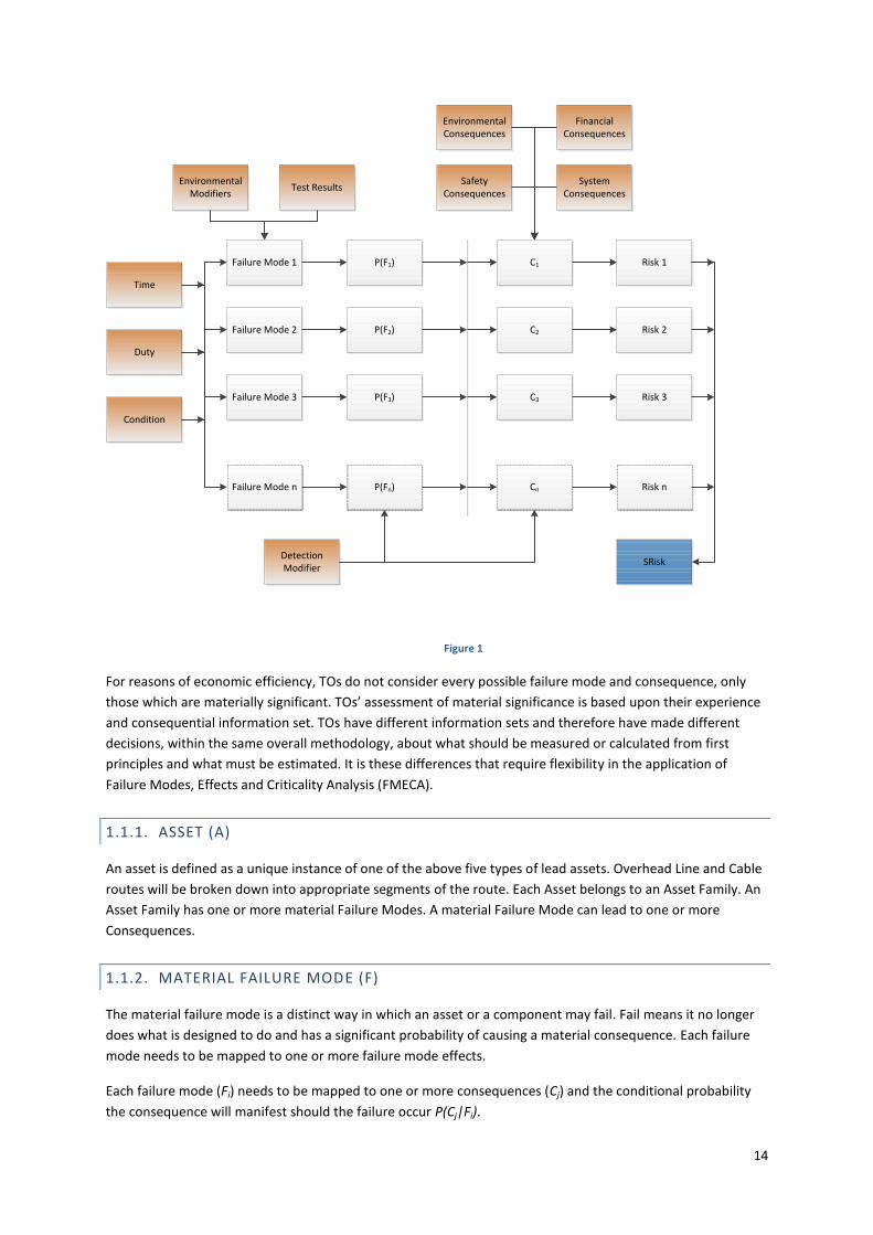
As shown in Figure 1 and Equation 3, the Asset Risk is the sum of the expected values of each consequence

associated with that asset. It is a function of the probability of each failure mode occurring, the probability of

consequences given a failure, the effectiveness of detection and the impact of each of the consequences.

14

Figure 1

For reasons of economic efficiency, TOs do not consider every possible failure mode and consequence, only

those which are materially significant. TOs’ assessment of material significance is based upon their experience

and consequential information set. TOs have different information sets and therefore have made different

decisions, within the same overall methodology, about what should be measured or calculated from first

principles and what must be estimated. It is these differences that require flexibility in the application of

Failure Modes, Effects and Criticality Analysis (FMECA).

1.1.1. ASSET (A)

An asset is defined as a unique instance of one of the above five types of lead assets. Overhead Line and Cable

routes will be broken down into appropriate segments of the route. Each Asset belongs to an Asset Family. An

Asset Family has one or more material Failure Modes. A material Failure Mode can lead to one or more

Consequences.

1.1.2. MATERIAL FAILURE MODE (F)

The material failure mode is a distinct way in which an asset or a component may fail. Fail means it no longer

does what is designed to do and has a significant probability of causing a material consequence. Each failure

mode needs to be mapped to one or more failure mode effects.

Each failure mode (Fi) needs to be mapped to one or more consequences (Cj) and the conditional probability

the consequence will manifest should the failure occur P(Cj|Fi).

Time

Duty

Condition

Failure Mode 1

Failure Mode 2

Failure Mode 3

Failure Mode n

P(F1)

P(F2)

P(F3)

P(Fn)

C1

C2

C3

Cn

Risk 1

Risk 2

Risk 3

Risk n

Environmental Modifiers

Detection Modifier

Environmental Consequences

Financial Consequences

Safety Consequences

System Consequences

SRisk

Test Results

15

However, where failure modes and consequences have a one-to-one mapping, this function is not required

and the Probability of Failure is equal to the Probability of Consequence.

1.1.3. PROBABILITY OF FAILURE P(F)

Probability of failure (P(Fi)) represents the probability that a Failure Mode will occur in the next time period. It

is generated from an underlying parametric probability distribution or failure curve. The nature of this curve

and its parameters (i.e. increasing or random failure rate, earliest and latest onset of failure) are provided by

the process known as Failure Mode and Effects Analysis (FMEA). The probability of failure is influenced by a

number of factors, including time, duty and condition as shown in section 2.3. Each TO will show the detailed

calculation steps to determine Probability of Failure within the appendices to this methodology.

1.1.4. PROBABILITY OF DETECTION AND ACTION P(D)

The probability that the failure mode is detected through inspection and action taken before there is a

consequence. The probability failure mode i is detected before the consequences arise is denoted by P(Di).

The probability of detection and action has been included at this stage for completeness. Further development

in this area could be considered in future iterations of the NOMs methodology; however, it is not currently

included within the TOs calculations.

1.1.5. CONSEQUENCE (C)

The monetised value for each of the underlying Financial, Safety, System and Environmental components of a

particular consequence e.g. Transformer Fire. Each Cj has one or more Fi mapped to it. A Consequence can be

caused by more than one Failure Mode, but a Consequence itself can only occur once during the next time

period. For example, an Asset or a particular component is only irreparably damaged once.

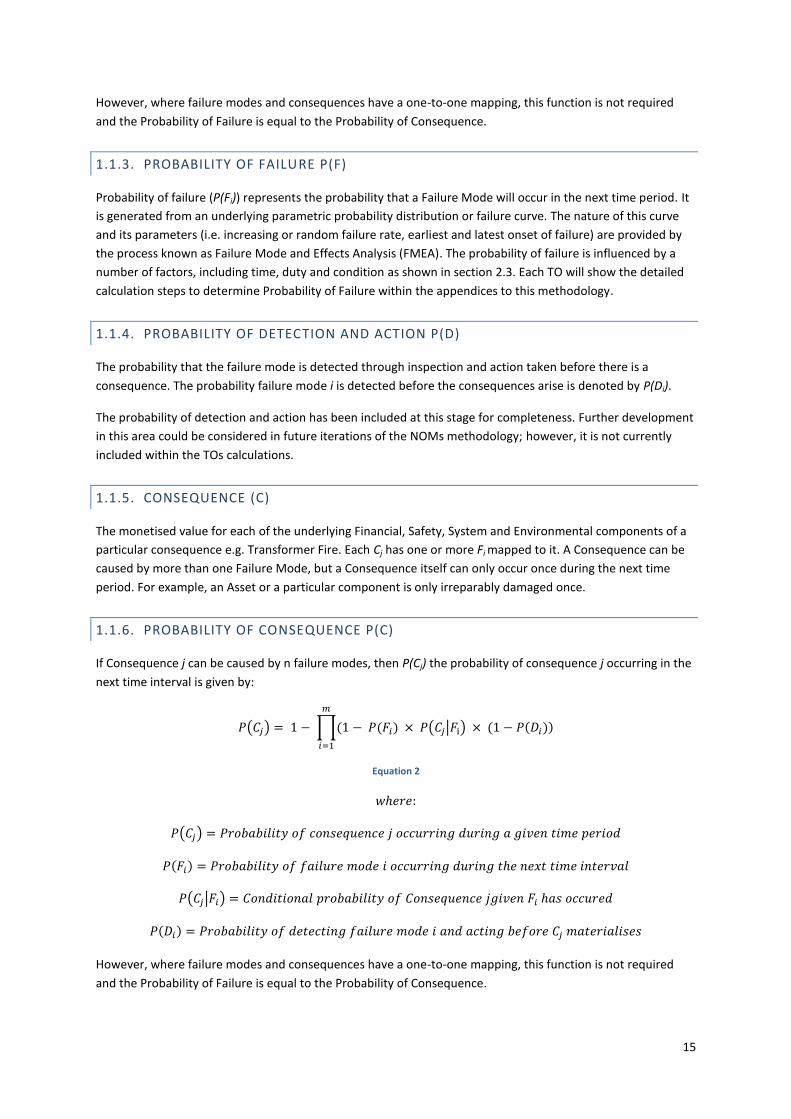
1.1.6. PROBABILITY OF CONSEQUENCE P(C)

If Consequence j can be caused by n failure modes, then P(Cj) the probability of consequence j occurring in the

next time interval is given by:

𝑃(𝐶𝑗) = 1 − ∏(1 − 𝑃(𝐹𝑖

𝑚

𝑖=1

) × 𝑃(𝐶𝑗|𝐹i) × (1 − 𝑃(𝐷𝑖))

Equation 2

𝑤ℎ𝑒𝑟𝑒:

𝑃(𝐶𝑗) = 𝑃𝑟𝑜𝑏𝑎𝑏𝑖𝑙𝑖𝑡𝑦 𝑜𝑓 𝑐𝑜𝑛𝑠𝑒𝑞𝑢𝑒𝑛𝑐𝑒 𝑗 𝑜𝑐𝑐𝑢𝑟𝑟𝑖𝑛𝑔 𝑑𝑢𝑟𝑖𝑛𝑔 𝑎 𝑔𝑖𝑣𝑒𝑛 𝑡𝑖𝑚𝑒 𝑝𝑒𝑟𝑖𝑜𝑑

𝑃(𝐹𝑖) = 𝑃𝑟𝑜𝑏𝑎𝑏𝑖𝑙𝑖𝑡𝑦 𝑜𝑓 𝑓𝑎𝑖𝑙𝑢𝑟𝑒 𝑚𝑜𝑑𝑒 𝑖 𝑜𝑐𝑐𝑢𝑟𝑟𝑖𝑛𝑔 𝑑𝑢𝑟𝑖𝑛𝑔 𝑡ℎ𝑒 𝑛𝑒𝑥𝑡 𝑡𝑖𝑚𝑒 𝑖𝑛𝑡𝑒𝑟𝑣𝑎𝑙

𝑃(𝐶𝑗|𝐹𝑖) = 𝐶𝑜𝑛𝑑𝑖𝑡𝑖𝑜𝑛𝑎𝑙 𝑝𝑟𝑜𝑏𝑎𝑏𝑖𝑙𝑖𝑡𝑦 𝑜𝑓 𝐶𝑜𝑛𝑠𝑒𝑞𝑢𝑒𝑛𝑐𝑒 𝑗𝑔𝑖𝑣𝑒𝑛 𝐹𝑖 ℎ𝑎𝑠 𝑜𝑐𝑐𝑢𝑟𝑒𝑑

𝑃(𝐷𝑖) = 𝑃𝑟𝑜𝑏𝑎𝑏𝑖𝑙𝑖𝑡𝑦 𝑜𝑓 𝑑𝑒𝑡𝑒𝑐𝑡𝑖𝑛𝑔 𝑓𝑎𝑖𝑙𝑢𝑟𝑒 𝑚𝑜𝑑𝑒 𝑖 𝑎𝑛𝑑 𝑎𝑐𝑡𝑖𝑛𝑔 𝑏𝑒𝑓𝑜𝑟𝑒 𝐶𝑗 𝑚𝑎𝑡𝑒𝑟𝑖𝑎𝑙𝑖𝑠𝑒𝑠

However, where failure modes and consequences have a one-to-one mapping, this function is not required

and the Probability of Failure is equal to the Probability of Consequence.

16

1.1.7. ASSET RISK

For a given asset (Ak), a measure of the risk associated with it is the Asset Risk, given by:

𝐴𝑠𝑠𝑒𝑡 𝑅𝑖𝑠𝑘(𝐴𝑘) = ∑𝑃(𝐶𝑗)

𝑛

𝑗=1

× 𝐶𝑗

Equation 3


𝑃(𝐶𝑗) = 𝑃𝑟𝑜𝑏𝑎𝑏𝑖𝑙𝑖𝑡𝑦 𝑜𝑓 𝑐𝑜𝑛𝑠𝑒𝑞𝑢𝑒𝑛𝑐𝑒 j 𝑜𝑐𝑐𝑢𝑟𝑟𝑖𝑛𝑔 𝑑𝑢𝑟𝑖𝑛𝑔 𝑎 𝑔𝑖𝑣𝑒𝑛 𝑡𝑖𝑚𝑒 𝑝𝑒𝑟𝑖𝑜𝑑

𝐶𝑗 = 𝑡ℎ𝑒 𝑚𝑜𝑛𝑒𝑡𝑖𝑠𝑒𝑑 𝐶𝑜𝑛𝑠𝑒𝑞𝑢𝑒𝑛𝑐𝑒 𝑗

𝑛 = 𝑡ℎ𝑒 𝑛𝑢𝑚𝑏𝑒𝑟 𝑜𝑓 𝐶𝑜𝑛𝑠𝑒𝑞𝑢𝑒𝑛𝑐𝑒𝑠 𝑎𝑠𝑠𝑜𝑐𝑖𝑎𝑡𝑒𝑑 𝑤𝑖𝑡ℎ 𝐴𝑠𝑠𝑒𝑡 𝑘

17

1.2. LEAD ASSETS

The following sections provide background and high level deterioration mechanisms for the lead assets.

Additional detail for these assets can be found in the TO appendices.

1.2.1. CIRCUIT BREAKERS

1.2.1.1. BACKGROUND

Circuit breakers are different to other lead assets as they generally have limited condition information on an

individual asset basis. To gather additional condition information on sub components which has the potential

to affect the end of life modifier, would require invasive work to assess the actual condition of a particular sub

component. It is undesirable to do so in the majority of situations as it would require a system outage.

Technically effective or cost justified diagnostic techniques, including continuous monitoring, are limited for

use on large populations and are not applicable for deterioration modes determining the end of life of most

types of existing circuit breaker. In addition, the deterioration age range is related to the equipment’s

environment, electrical and mechanical duty, maintenance regime and application.

In this methodology we therefore introduce a family specific deterioration component to the end of life

modifier formula to account for missing condition information. Assignment to particular family groupings is

through identification of similar life limiting factors. Family groupings are broadly split into interrupter

mechanism type.

Known deterioration modes have been determined by carrying out forensic analysis of materials and

components during replacement, refurbishment, maintenance and failure investigation activities or following

failures. The output of the forensic analysis reports has been used to both inform and update the relevant

deterioration models. Anticipated technical asset lives are based on the accumulated Engineering knowledge

of TO’s Defect, Failure statistics and manufacturer information. The method for mapping this knowledge to the

end of life curve was presented in the functional modes and affects analysis section.

1.2.1.2. DETERIORATION

Circuit breakers are made up of large number sub-components. These sub-components deteriorate at

different rates, are different in relation to their criticality to the circuit breaker function and finally have

different options regarding intervention

Although there is a correlation between age and condition, it has been observed that there is a very wide

range of deterioration rates for individual units. The effect of this is to increase the range of circuit breaker

condition with age, some circuit breakers becoming unreliable before the anticipated life and some showing

very little deterioration well after that time.

1.2.1.3. AIR-BLAST CIRCUIT BREAKER TECHNOLOGY

As Air-Blast Circuit Breaker (ABCB) families approach their end of life an assessment is made regarding the

relative economic impact of replacement or refurbishment taking into account factors such as technological

complexity, population size and ongoing asset management capability for the design. Since most ABCB families

are no longer supported by their original equipment manufacturer, the cost and feasibility of providing parts,

skilled labour and ongoing technical support must be factored into the total cost of refurbishment. For this

reason, refurbishment may only be cost-effective for certain, large family types. For small families, the cost of

18

establishing a refurbishment programme and maintaining appropriate knowledge and support will most often

favour replacement.

Using the above approach refurbishment has, in selected cases, proven to be an effective way to extend the

Anticipated Asset Life (AAL) for Conventional Air-Blast (CAB) and Pressurised head (PAB) ABCBs.

The replacement of ABCBs is considered alongside the remaining lifetime of the associated site air system. If

removal of the last ABCBs at a site allows the site air system to be decommissioned, early switchgear

replacement may be cost beneficial when weighed against further expenditure for air system replacement

and/or on-going maintenance.

1.2.1.4. OIL CIRCUIT BREAKER TECHNOLOGY

The life-limiting factor of principal concern is moisture ingress and the subsequent risk of destructive failure

associated with the BL barrier bushing in bulk Oil Circuit Breakers (OCBs). A suitable replacement bushing has

been developed that can be exchanged when moisture levels reach defined criteria, but at a high cost to the

extent that is not economical to replace many bushings using this technology. Risk management of bushings

has been achieved by routine oil sampling during maintenance, subsequent oil analysis and replacement of

bushings where required. On this basis the AAL for this technology has been extended and detailed plans for

replacement or refurbishment remain to be developed.

1.2.1.5. SF6 GAS CIRCUIT BREAKER TECHNOLOGY

The bulk of the Gas Circuit Breaker population (GCB) is relatively young compared to its AAL, and therefore

many have not required replacement. A similar process to that followed for the ABCB families is being

undertaken to identify refurbishment (i.e. life extension) opportunities. Where this is not technically-feasible

or cost-effective, replacement is planned.

The GCB population includes a large number of small families, with variants and differing operating regimes,

and so the identification of large-scale refurbishment strategies may not be cost-effective. Technical and

economic evaluation as well as further development of refurbishment strategies will take place.

A significant number of SF6 circuit-breakers which are installed on shunt reactive compensation are subject to

very high numbers of operations (typically several hundred per year). The “end of life” of these circuit-breakers

is likely to be defined by number of operations (“wear out”) rather than age related deterioration. To assist

with asset replacement planning, these circuit-breakers have been assigned a reduced asset life in this

document based on a prediction of their operating regime. Different asset lives have been assigned depending

on the circuit breaker mechanism type and/or if the circuit breaker has been reconditioned; in each case the

asset life is based on an operating duty of 300 operations per year. It is currently proposed to recondition most

types of high duty reactive switching circuit breaker when they have reached their anticipated asset life based

on the number of operations they have performed. A more detailed asset specific strategy for replacement or

refurbishment of these categories of circuit-breakers is being developed in terms of the actual number of

operations and their forecast operating regime.

19

1.2.2. TRANSFORMERS AND REACTORS

1.2.2.1. BACKGROUND

Transformers and reactors share similar end of life mechanisms since they are both based on similar

technologies. The same scoring method is therefore applied to calculate the End of Life modifier. For simplicity

within this section the term transformer is used to mean both transformer and reactor.

Transformers are assigned an end of life modifier according to the condition inferred from diagnostic results,

the service history, and post mortem analysis of other similar transformers.

The health of the overall transformer population is monitored to ensure that replacement/refurbishment

volumes are sufficient to maintain sustainable levels of reliability performance, to manage site operational

issues associated with safety risks and to maintain or improve environmental performance in terms of oil

leakage.

The process by which transformers are assigned an end of life modifier relies firstly on service history and

failure rates specific to particular designs of transformers and secondly on routine test results such as those

obtained from Dissolved Gas Analysis (DGA) of oil samples. When either of these considerations gives rise to

concern, then where practicable, special condition assessment tests (which usually require an outage) are

performed to determine the appropriate end of life modifier. Special condition assessment may include the

fitting of a continuous monitoring system and the analysis of the data to determine the nature of the fault and

the deterioration rate.

The elements to be taken into account when assigning an end of life modifier are:

1. Results of routine condition testing

2. Results of special condition assessment tests

3. Service experience of transformers of the same design, and forensic examination of decommissioned

transformers

4. Results of continuous monitoring where available

The following additional condition indications shall be taken into account when deciding the

repair/replacement/refurbishment strategy for a particular transformer:

1. Condition of oil

2. Condition of bushings

3. Condition of coolers

4. Rate of oil loss due to leaks

5. Condition of other ancillary parts and control equipment

6. Availability of spare parts particularly for tap-changers

20

1.2.2.2. TRANSFORMER AND REACTOR DETERIORATION

Thermal ageing of paper is the principal life limiting mechanism for transformers which will increase the failure

rate with age. This failure mechanism is very dependent on design and evidence from scrapped transformers

indicates a very wide range of deterioration rates. Knowledge of the thermal ageing mechanism, other ageing

mechanisms and the wide range of deterioration rates are used to define the technical asset lives for

transformers.

In addition to the above fundamental limit on transformer service life, Experience has shown that a number of

transformer design groups have inherent design weaknesses which reduce useful service life

The condition of Transformers can be monitored through routine analysis of dissolved gases in oil, moisture

and furfural content together with routine maintenance checks. Where individual test results, trends in test

results or family history give cause for concern, specialist diagnostics are scheduled as part of a detailed

condition assessment. Where appropriate, continuous monitoring will also be used to determine or manage

the condition of the transformer.

Methods exist to condition assess transformers and indicate deterioration before failure, however the time

between the first indications of deterioration and the transformer reaching a state requiring replacement is

varied and can depend on factors such as the failure mechanism, the accuracy of the detection method, and

the relationship between system stress and failure. For this reason the transformer models periodically

require updating (supported by evidence from forensic analysis) as further understanding of deterioration

mechanisms is acquired during the transformer life cycle.

1.2.2.3. INSULATING PAPER AGEING

The thermal ageing of paper insulation is the primary life-limiting process affecting transformers and reactors.

The paper becomes brittle, and susceptible to mechanical failure from any kind of shock or disturbance.

Ultimately the paper will also carbonise and cause turn to turn failure, both mechanisms leading to dielectric

failure of the transformer. The rate of ageing is mainly dependent upon the temperature and moisture

content of the insulation. Ageing rates can be increased significantly if the insulating oil is allowed to

deteriorate to the point where it becomes acidic.

The thermal ageing of paper insulation is a chemical process that liberates water. Any atmospheric moisture

that enters the transformer during its operation and maintenance will also tend to become trapped in the

paper insulation. Increased moisture levels may cause dielectric failures directly or indirectly due to formation

of gas bubbles during overload conditions.

The paper and pressboard used in the construction of the transformer may shrink with age which can lead to

the windings becoming slack. This compromises the ability of the transformer windings to withstand the

electromagnetic forces generated by through fault currents. Transformer mechanical strength may be

compromised if it has experienced a number of high current through faults during its lifetime and the internal

supporting structure has been damaged or become loose.

21

End of life as a result of thermal ageing will normally be supported by evidence from one or more of the

following categories:

1. Forensic evidence (including degree of polymerisation test results) from units of similar design and

load history

2. High and rising furfural levels in the oil

3. High moisture content within the paper insulation

4. Evidence of slack or displaced windings (frequency response tests or dissolved gas results)

1.2.2.4. CORE INSULATION

Deterioration of core bolt and core-to-frame insulation can result in undesirable induced currents flowing in

the core bolts and core steel under certain load conditions. This results in localised overheating and risk of

Buchholz alarm/trip or transformer failure as free gas is generated from the localised fault. It is not normally

possible to repair this type of fault without returning the transformer to the factory. Evidence of this end of

life condition would normally be supported by dissolved gas results together with forensic evidence from

decommissioned transformers of similar design. Insertion of a resistor into the core earth circuit can reduce or

eliminate the induced current for a period of time.

1.2.2.5. THERMAL FAULT

Transformers can develop localised over-heating faults associated with the main winding as a result of poor

joints within winding conductors, poor oil-flow or degradation of the insulation system resulting in restrictions

to oil flow. This is potentially a very severe fault condition. There is not normally a repair for this type of fault

other than returning the transformer to the factory. Evidence of this end of life condition would normally be

supported by dissolved gas results together with forensic evidence from decommissioned transformers of

similar design.

1.2.2.6. WINDING MOVEMENT

Transformer windings may move as a result of vibration associated with normal operation or, more commonly,

as a result of the extreme forces within the winding during through fault conditions. The likelihood of winding

movement is increased with aged insulation as outlined above. Where evidence of winding movement exists,

the ability of the transformer to resist subsequent through faults is questionable and therefore the unit must

be assumed not to have the strength and capability to withstand design duty and replacement is warranted.

There is no on-site repair option available for this condition. Winding movement can be detected using

frequency response test techniques and susceptibility to winding movement is determined through failure

evidence and evidence of slack windings through dissolved gas results.

1.2.2.7. DIELECTRIC FAULT

In some circumstances transformers develop dielectric faults, where the insulation degrades giving concern

over the ability of the transformer to withstand normal operating voltages or transient overvoltage. Where an

internal dielectric fault is considered to affect the main winding insulation, irreparable damage is likely to

ensue. This type of condition can be expected to worsen with time. High moisture levels may heighten the

risk of failure. Evidence of a dielectric problem will generally be based on operational history and forensic

investigations from units of similar design, supported by dissolved gas results. Various techniques are

available to assist with the location of such faults, including partial discharge location techniques. If evidence

22

of an existing insulation fault exists and location techniques cannot determine that it is benign, then the

transformer should be considered to be at risk of failure.

1.2.2.8. CORROSIVE OIL

In certain cases high operating temperatures combined with oil containing corrosive compounds can lead to

deposition of copper sulphide in the paper insulation, which can in turn lead to dielectric failure. This

phenomenon may be controlled by the addition of metal passivator to the oil, however experience with this

technique is limited and so a cautious approach to oil passivation has been adopted. Regeneration or

replacement of the transformer oil may be considered for critical transformers or where passivator content is

consumed quickly due to higher operating temperatures.

23

1.2.3. UNDERGROUND CABLES

1.2.3.1. BACKGROUND

Cable system replacements are programmed so that elements of the cable systems are replaced when the

safety, operational or environmental risks of continued operation meet defined criteria.

Replacement of cable systems are based on a number of metrics including age. These metrics only include a

few condition related components since there is limited information that can be obtained on how deteriorated

a cable actually is. Further condition information could be obtained by digging up and taking samples of a

cable, but this is not practical, would be costly and could also cause further failures. Metrics such as the cost of

repairs is taken into account when determining if a cable has reached the end of its life. While this isn’t the

most desirable metric from an analytical perspective, it does reflect historical practice and is justifiable from a

consumer value perspective.

The factors to be taken into account when determining an end of life modifier are:

1. Historical environmental performance

2. Historical unreliability

3. Risk of tape corrosion or sheath failure

4. Results of condition assessment and other forensic evidence

5. Service experience of cable systems of similar design

6. Number of defect repairs

7. Number of cable faults

8. Duty in terms of how much time annually a cable is running at or above its designed rating

9. Bespoke nature and issues associated with specific cable systems

24


End of technical life will generally be due to the deterioration of the main cable system; this may be associated

with either mechanical or electrical integrity or withstand capability.

With the exception of cables vulnerable to reinforcing tape corrosion and cables where a known

manufacturing defect has occurred (e.g. lead sheath deterioration), cable systems have generally given reliable

operation and there is limited experience of long term deterioration mechanisms.

Cables can be split broadly into two classes for the purposes of understanding the end of life of this asset class,

these are fluid filled cables and solid dielectric cables. In general the cable circuit will only meet the criteria for

replacement where refurbishment as described above will not address condition and performance issues and

guarantee compliance with statutory requirements.

1.2.3.3. END OF LIFE MECHANISMS AFFECTING BOTH TYPES OF CABLES

1.2.3.3.1. LEAD AND ALUMINIUM SHEATH DETERIORATION

Fatigue and intercrystalline cracking, and defects introduced during manufacture can cause oil leaks to

develop. It is not generally possible to predict when a given cable section will fail as a result of this failure

mode. Local repairs are not generally effective as sheath deterioration is usually distributed along the cable.

End-of-life is reached where sheath deterioration is resulting in significant and widespread oil-loss (relative to

duties in respect of recognised code of practice) along the cable length.

1.2.3.3.2. BONDING SYSTEM

Water ingress to link boxes causes deterioration of cross-bonding systems and leaves the link box and its

sheath voltage limiters (SVLs) vulnerable to explosive failure under fault conditions. Specific evidence shall be

gathered through condition assessment to support end-of-life determination. This issue will in general be

addressed by replacement of specific components during circuit refurbishment activity or enhanced routine

maintenance.

1.2.3.3.3. COOLING SYSTEM

The life of a cable’s cooling system is much shorter than the lifetime of the overall cable asset. Therefore mid-

life intervention maybe required to replace the cable cooling system components. While this is not the end of

the life of the cable it is an important consideration as the cable is not able to do what it was designed to do

with a failed cooling system. Cooling systems tend to be unique to each cable route. Loss of the cooling

capacity can typically reduce circuit rating by 40%. Most problems are experienced with the original control

systems which are now obsolete. Aluminium cooling pipes are vulnerable to corrosion and plastic pipes are

vulnerable to splitting, which can result in water leaks. Cooling control system and pumping equipment will

also require replacement prior to the main cable system in line with circuit specific assessment. In general

cooling pipework should be managed through maintenance to achieve the asset life of the main cable system.

25

1.2.3.4. FLUID FILLED CABLE END OF LIFE MECHANISMS

1.2.3.4.1. REINFORCING TAPE CORROSION

Reinforcing tapes are used to retain the oil pressure for cables with lead sheaths. Corrosion of the tapes in

certain early BICC cables and AEI cables results in the tapes breaking, the sheath splitting and consequential oil

leaks. We are developing methods for predicting failure using corrosion rates determined through sampling in

combination with known operating pressures, and also using degradation mechanism models. Local repairs are

not considered effective mitigation as corrosion is usually distributed along the cable. End-of-life of the cable

system is in advance of widespread predicted tape failure. The lead times for cable replacement schemes are

considerably greater than the time to deteriorate from broadly acceptable to unacceptable cable system

performance for this failure mode. This implies that pre-emptive action is required to minimise the likelihood

of failure occurring. Acceptable performance is where the cable can be repaired on an ad-hoc basis;

unacceptable performance is where the corrosion is distributed along a significant number of sections of the

route.

1.2.3.4.2. STOP JOINT DETERIORATION

Stop-joint failure presents significant safety, reliability and environmental risk. End-of-life for stop joints will be

justified based upon oil-analysis data or forensic evidence from similar designs removed from service. Stop

joint deterioration can be addressed via refurbishment and would not alone drive replacement of the cable

system.

1.2.3.4.3. CABLE JOINT DETERIORATION

In general cable joint deterioration can be addressed via refurbishment and would not alone drive

replacement of the joint or cable system.

1.2.3.4.4. OIL-ANCILLARIES

Corrosion of oil tanks, pipework and connections, and pressure gauges can result in oil leaks and incorrect

operation of the ancillaries. Specific evidence shall be gathered through condition assessment to support end-

of-life determination. This issue will in general be addressed by replacement of specific components during

circuit refurbishment activity or enhanced routine maintenance.

1.2.3.4.5. ENVIRONMENTAL CONSIDERATIONS

TO’s have a statutory obligation to comply with the Water Resources Act 1991/Water Resources (Scotland) Act

2013 and to fulfil their commitments with respect to its Environmental Statement. Utilities demonstrate

compliance with the requirement of the Act through adherence to the guidance provided.

A factor to consider in determining end of technical life is when it is no longer reasonably practicable to

comply with the requirements of the above legislation and guidance, and maintain a sustainable level of circuit

availability.

26

1.2.3.4.6. SOLID XLPE FILLED CABLE END OF LIFE MECHANISMS:

These cables have been installed at 132kV and 275kV for some years. There is limited service experience at

400kV. Provided high standards of manufacture and installation are available, the risk of early-life failures will

be avoided. No end of life mechanism has yet been identified. The long-term deterioration mechanisms would

benefit from further research and development.

27

1.2.4. OVERHEAD LINES

1.2.4.1. GENERAL APPROACH

Routes are fully refurbished, or have critical components replaced, to maintain reliability (including a level of

resilience to extreme weather conditions), operational risk and safety performance. In addition conductors

should retain sufficient residual mechanical strength to facilitate safe replacement by tension stringing

methods at end of life.

Technical asset lives for OHL components in various environments have been predicted using historical

condition information from previous OHL replacement schemes, condition samples taken on existing assets,

and an understanding of deterioration mechanisms.

Scoring assessments are made on sections of circuit that are typically homogenous in conductor type,

installation date and environment.


1.2.4.1.1. CONDUCTORS

Conductor end of life condition is a state where the conductor no longer has the mechanical strength (both

tensile and ductility) required to support the combination of induced static and environmental loads.

Two main deterioration mechanisms exist:

1. Corrosion, primary cause pollution either saline or industrial

2. Wind induced fatigue, common types

a. Aeolian vibration (low amplitude high frequency oscillation 5 to 150 Hz)

b. sub-conductor oscillation (bundles conductors only) produced by forces from the shielding

effect of windward sub-conductors on their leeward counterparts

c. galloping (high-amplitude, low-frequency oscillation)

d. wind sway

Conductor fatigue is usually found at clamp positions where the clamp allows more interstrand motion within

the conductor, leading to fretting of the internal layers. Loss of strand cross-section follows, then fatigue

cracking, and finally strand breakage. This form of degradation is generally the life-limiting factor for quad

bundles, clamping positions on twin bundles can also be affected

Conductor corrosion is also usually found at clamp positions. Interwoven conductor strands open up at these

points allowing for easier ingress of corroding chlorides, sulphates and moisture etc. The zinc galvanising of the

core wires is corroded, eventually exposing the underlying steel. A galvanic corrosion cell is then created

where the aluminium wire is sacrificial. The loss of cross section of aluminium leads to greater heat transfer to

the steel core increasing the risk of core failure. Additionally, some spacer clamps with elastomer bushings that

contain carbon and have a low resistance also lead to galvanic corrosion of aluminium strands, reducing

thickness, strength and ductility.

In addition in rare instances, end of life may be advanced due to an unexpected load or events such as

extreme wind ice or heat which over load/stresses the conductor beyond its design capability. Quality of the

original manufacturing could also be an issue (galvanising defects) but there is not much evidence for this in

our conductor condition assessment data.

28

1.2.4.1.2. INSULATORS

The end of life occurs when the increased risk of flashover (loss of dielectric strength) reaches an unacceptable

level due to condition, which may or may not result in mechanical failure of the string, or a decrease in

mechanical strength due to corrosion of the steel pin.

1.2.4.1.3. FITTINGS - SPACERS, SPACER DAMPERS AND VIBRATION DAMPERS

The functional end of life of spacers, spacer dampers and vibration dampers occurs at the point at which the

conductor system is no longer protected, and conductor damage starts to occur.

These items are utilised to protect the conductor system from damage. The main deterioration mechanism is

wear or fatigue induced through conductor motion. Corrosion in polluted environments can also be an issue

particularly inside clamps

Wear damage to trunnions and straps of suspension clamps occurs due to conductor movement. The wear has

been greatest in areas of constant wind, i.e. higher ground, flat open land and near coasts. For quad lines, in

particular at wind exposed sites, wear can be extensive and rapid failures of straps, links, shackles and ball-

ended eye links can occur. This is one of the best indicators of line sections subject to sustained levels of wind

induced oscillation and hence where future conductor damage is likely to become a problem.

Most conductor joints for ACSR have been of the compression type, although bolted joints are used in

jumpers. Overheating joints can arise from inadequate compression along the length of the joint, mainly due

to either poor design or installation problems. These allow moisture penetration and oxidation of the internal

aluminium surfaces between the joint and conductor. The resistive aluminium oxide reduces the paths for

current flow and may cause micro-arcing within the joint. The consequence of this deterioration is that the

joint becomes warm which further increases the rate of oxidation. Over a period of time, the resistive paths

can result in excess current flowing in the steel core of the conductor, which can then overheat and rupture.

1.2.4.1.4. SEMI-FLEXIBLE SPACERS

These are fitted in the span and the semi-flexibility comes from either elastomer liners, hinges or stranded

steel wire depending on the manufacturer. End of life is defined by perishing of the elastomer lining or

broken/loose spacer arms. These allow for excessive movement of the conductor within the clamp leading to

severe conductor damage in small periods of time (days to months, depending on the environmental input).

The elastomer lining of the Andre spacer type also causes corrosion of conductor aluminium wires due to its

carbon content and subsequent galvanic corrosion. A common finding of conductor samples at these positions

is strands with significantly poorer tensile and torsional test results. This is a hidden condition state unless it

manifests in broken conductor strands that are visible on inspection.

Replacement of these spacers has been necessary on routes that are heavily wind exposed at approximately

25 years. There are many examples still in service beyond their anticipated life of 40 years where visual end of

life characteristics have not yet been met. As the condition of the associated conductor within or near the

clamp can remain hidden, certain families of this type of spacer such as the ‘Andre’ are identified for the

increased risk they pose to conductor health.

29

1.2.4.1.5. SPACER DAMPERS

As the service history of spacer dampers is limited, extensive data on their long-term performance and end of

life is not yet available. The spacer arms are mounted in the spacer body and held by elastomer bushes. This

increased flexibility should provide the associated conductor system with more damping and greater resilience

to wind induced energy. End of life criteria will be defined by broken/loose spacer arms that allow for

excessive movement of the conductor/clamp interface.

1.2.4.1.6. VIBRATION DAMPERS

Stockbridge dampers have always been used for the control of Aeolian vibration, a minimum of one damper

being installed at each end of every span on each subconductor. For long spans (where specified by the

manufacture) two or more may be used. End of life is defined by loss of damping capability which is visually

assessed in the amount of ‘droop’ in and wear of the messenger cable between damper bells. The useful life of

a damper is constrained by wind energy input and corrosion of the messenger wire connection with the

damper bells. In areas of high wind exposure we have evidence that dampers have required replacement after

10 to 15 years. There are however many more examples of dampers operating beyond their anticipated life

with no visual signs of end of life.

1.2.4.1.7. TOWERS

Corrosion and environmental stress are life-limiting factors for towers. The end of life of a whole tower is the

point at which so many bars require changing that it is more economical to replace the whole tower.

Degradation of foundations is another life-limiting factor for towers.

30

2. PROBABILITY OF FAILURE

2.1. PROCESS FOR FMEA

The process for identifying failure modes uses component studies for each asset class to understand the asset

risk.

For each component, each failure mode (that is each component) is assessed to determine:

Detection: effectiveness of detection, where applicable

Event: all possible events including the probability of a particular event. It is connected with each

failure mode, whichever type that failure mode may be

Probability of Failure

Type of Failure Mode (P-F, utilisation, random)

In order to establish an asset’s likelihood of failure, Failure Modes and Effects Analysis (FMEA) is used. FMEA is

a structured, systematic technique for failure analysis. It involves studying components, assemblies and

subsystems to identify failure modes, their causes and effects. The use of FMEA in this context aims to

examine the effectiveness of the TOs’ current risk management by considering these key elements relating to

potential failure modes:

What are the effects or consequences of the failure mode?

How often might the failure mode occur?

How effective is the current detection?

How effective are the interventions for the failure mode?

Many assets in transmission networks are asset systems (combinations of assets). FMEA views the asset as an

assembly of ‘items’, being the part of the asset that performs a defined function. In terms of identifying failure

modes, the items under consideration are usually sub-assemblies, but there may be discrete components.

Some of the asset categories are single asset types which can be separated into an integrated set of items.

To determine risk it is necessary to identify the consequences of each potential failure event. The addition of

consequence considerations to FMEA leads to FMECA.

Some illustrative guidance is provided by BS EN 60812 and section 5.2.5 stresses the importance of considering

both local and system effects – recognising that the effects of a component failure are rarely limited to the

component itself.

In a highly-meshed system, such as a transmission network, consideration of system effects becomes

paramount. Unfortunately, traditional FMECA analysis (as described in BS EN 60812) does not enable such

analysis, relying as it does on non-tradeable “criticality scores”. To comply with the NOMs requirements, a

much more comprehensive system of consequence evaluation must be derived, leading to a transparent,

objective and tradeable measure of risk.

31

2.1. UNDERSTANDING FAILURE CAUSE TYPES ON TO ASSETS

There are five basic underlying types of failure:

1. Time based failure (Potential to Functional failure)

The patterns of failure are predictable with an interval between initiation (potential) to failure.

Inspection activities may be available to identify these. These are represented within the model with

an earliest and latest expected onset of the failure based on the time that has elapsed following the

last intervention (for example, maintenance activity) which addresses the particular failure

2. Utilisation failure

Failure is based on duty with a predictable ‘useful life’ for the component. A preventative intervention

can be undertaken, if this useful life is understood, which can be scheduled before failure occurs. For

example, these asset types may have a known number of operations and are represented in the

model by the number of expected operations to failure since the last intervention that addresses the

particular failures

3. Random failure

These failure modes will have a constant failure rate, usually expressed as a percentage per annum

for the population

4. Hidden failure

These are failure modes that cannot be detected but which exist and may require the occurrence of a

failure in order for them to be revealed. Initially these can only be addressed through reactive

interventions. They may be specific to the asset but may apply to a family of assets as a type defect or

a deterioration mode that had not previously been understood

5. Asset specific failure

Some assets are not able to be influenced by maintenance. For example a design weakness may

become apparent for a particular family of assets.

To avoid unnecessary levels of analysis, section 5.2.4 of BS EN 60812 recommends that the most likely causes

for each failure mode should be identified. Therefore, rather than identifying every single possible cause for all

failure modes, the level of detail should be reflective of the failure mode effects and their severity. The more

severe the effects the more accurate the identification and description to prevent unnecessary effort to failure

causes with little effect. The failure cause may usually be determined from analysis of failed failures, test units

or expert opinion.

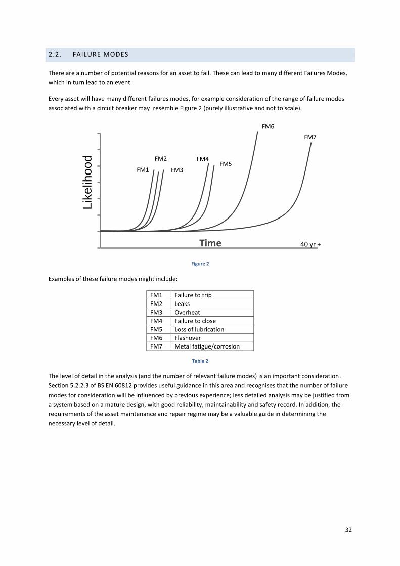
32

2.2. FAILURE MODES

There are a number of potential reasons for an asset to fail. These can lead to many different Failures Modes,

which in turn lead to an event.

Every asset will have many different failures modes, for example consideration of the range of failure modes

associated with a circuit breaker may resemble Figure 2 (purely illustrative and not to scale).

Figure 2

Examples of these failure modes might include:

FM1 Failure to trip

FM2 Leaks

FM3 Overheat

FM4 Failure to close

FM5 Loss of lubrication

FM6 Flashover

FM7 Metal fatigue/corrosion

Table 2

The level of detail in the analysis (and the number of relevant failure modes) is an important consideration.

Section 5.2.2.3 of BS EN 60812 provides useful guidance in this area and recognises that the number of failure

modes for consideration will be influenced by previous experience; less detailed analysis may be justified from

a system based on a mature design, with good reliability, maintainability and safety record. In addition, the

requirements of the asset maintenance and repair regime may be a valuable guide in determining the

necessary level of detail.

0

10

20

30

40

50

60

70

Text 1Text 2Text 3Text 4Text 5Text 6Text 7Text 8

Ris

k

Time

FM1

FM2

FM3

FM4 FM5

FM6

FM7

40 yr +

Lik

elih

oo

d

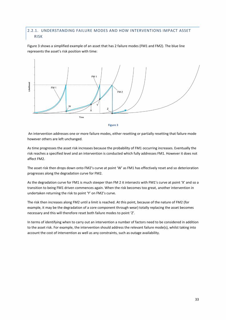
33

2.2.1. UNDERSTANDING FAILURE MODES AND HOW INTERVENTIONS IMPACT ASSET

RISK

Figure 3 shows a simplified example of an asset that has 2 failure modes (FM1 and FM2). The blue line

represents the asset’s risk position with time:

Figure 3

An intervention addresses one or more failure modes, either resetting or partially resetting that failure mode

however others are left unchanged.

As time progresses the asset risk increases because the probability of FM1 occurring increases. Eventually the

risk reaches a specified level and an intervention is conducted which fully addresses FM1. However it does not

affect FM2.

The asset risk then drops down onto FM2’s curve at point ‘W’ as FM1 has effectively reset and so deterioration

progresses along the degradation curve for FM2.

As the degradation curve for FM1 is much steeper than FM 2 it intersects with FM1’s curve at point ‘X’ and so a

transition to being FM1 driven commences again. When the risk becomes too great, another intervention in

undertaken returning the risk to point ‘Y’ on FM2’s curve.

The risk then increases along FM2 until a limit is reached. At this point, because of the nature of FM2 (for

example, it may be the degradation of a core component through wear) totally replacing the asset becomes

necessary and this will therefore reset both failure modes to point ‘Z’.

In terms of identifying when to carry out an intervention a number of factors need to be considered in addition

to the asset risk. For example, the intervention should address the relevant failure mode(s), whilst taking into

account the cost of intervention as well as any constraints, such as outage availability.

Lik

elih

oo

d

34

2.2.2. DETECTING FAILURE MODES

There are a number of techniques that can be used to detect certain failure modes.

Table 3

2.2.3. EVENTS RESULTING FROM A FAILURE MODE

Each failure mode may result in one or more events. These are categorised in a hierarchy of failure mode

events in terms of the impact.

The events are categorised in a hierarchy of failure mode consequences in terms of the impact of failurewhich

are comparable across the asset types , an example of which is shown in Table 4.

Event

No Event

Environment Noise

Reduced Capability

Alarm

Unwanted Alarm + Trip

Transformer Trip

Reduced Capability + Alarm + Trip

Fail to Operate + Repair

Reduced Capability + Alarm + Loss of Voltage Control + Fail to Operate

Overheating (will trip on overload)

Cross Contamination of Oil

Alarm + Damaged Component (Tap Changer) No Trip

Alarm + Trip + Damaged Component (Tap Changer)

Alarm + Trip + Tx Internal Damage

Alarm + Trip + Damage + State Requiring Replacement (Asset Replacement)

Alarm + Trip + Disruptive Failure + External Damage (danger) + Replacement

Alarm + Trip + Disruptive Failure + External Damage (danger) + Replacement+ Transformer Fire

Table 4

Detection Technique Activity

Periodic inspection Routine inspection of asset at set intervals.

Alarm/indication/ metering

Automatic systems that monitor certain parameters on equipment and provide an automatic alert, e.g. cable oil pressure monitoring detects the possibility of an oil leak.

Sample monitoring Periodic sampling to establish specific parameters to determine health of asset, e.g. oil sampling on transformers.

Continuous monitoring

Monitoring equipment installed on specific assets whereby data about their health is recovered, logged, trended and monitored autonomously. Alerts are generated when thresholds are breached, or when a parameter exceeds X% in a specified time frame, e.g. Mobile Transformer Assessment Clinic.

Periodic operation Planned operation to ensure that the asset/components/mechanisms function as expected, e.g. periodic operation of circuit breakers.

35

The same failure mode may result in different events. For example, Table 5 shows the potential events for the

dielectric failure of a transformer bushing.

Asset Type Item Function Failure Mode Cause Event

Transformer Bushing

Carries a conductor through a

partition such as a wall or tank and insulates it

therefrom

Dielectric failure (oil, oil

impregnated paper, resin imp paper,

resin bonded paper, solid cast

resin, SF6)

Water ingress/ treeing (partial

discharge)

Alarm + Trip + Disruptive Failure + External Damage (danger) + Replacement+ Transformer Fire

Alarm + Trip + Disruptive Failure + External Damage (danger) + Replacement

Alarm + Trip + Internal Damage

Alarm + Trip

Table 5

In all instances of this failure mode the transformer will trip and a component will be damaged, which will

require investigation and repair. However, there is also a 50% chance of the transformer failing disruptively,

i.e. that the transformer will need to be replaced rather than simply repaired.

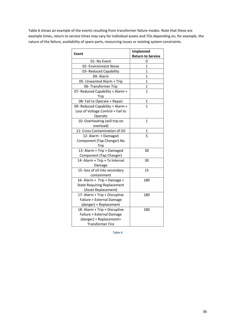
36

Table 6 shows an example of the events resulting from transformer failure modes. Note that these are

example times, return to service times may vary for individual assets and TOs depending on, for example, the

nature of the failure, availability of spare parts, resourcing issues or existing system constraints.

Event Unplanned Return to Service

01- No Event 0

02- Environment Noise 1

03- Reduced Capability 1

04- Alarm 1

05- Unwanted Alarm + Trip 1

06- Transformer Trip 1

07- Reduced Capability + Alarm + Trip

1

08- Fail to Operate + Repair 1

09- Reduced Capability + Alarm + Loss of Voltage Control + Fail to

Operate

1

10- Overheating (will trip on overload)

1

11- Cross Contamination of Oil 1

12- Alarm + Damaged Component (Tap Changer) No

Trip

5

13- Alarm + Trip + Damaged Component (Tap Changer)

30

14- Alarm + Trip + Tx Internal Damage

30

15- loss of oil into secondary containment

15

16- Alarm + Trip + Damage + State Requiring Replacement

(Asset Replacement)

180

17- Alarm + Trip + Disruptive Failure + External Damage (danger) + Replacement

180

18- Alarm + Trip + Disruptive Failure + External Damage (danger) + Replacement+

Transformer Fire

180

Table 6

37

2.3. PROBABILITY OF FAILURE

The determination of Probability of Failure (PoF) can be especially challenging for highly reliable assets. BS EN

60812 provides useful guidance on how to develop an estimate for PoF.

Section 5.2.9 of BS EN 60812 recognises that it is very important to consider the operational profile

(environmental, mechanical, and/or electrical stresses applied) of each component that contributes to its

probability of occurrence. This is because the component failure rates, and consequently failure rate of the

failure mode under consideration, in most cases increase proportionally with the increase of applied stresses

with the power law relationship or exponentially. Probability of occurrence of the failure modes for the design

can be estimated from:

Data from the component life testing

Available databases of failure rates

Field failure data

Failure data for similar items or for the component class

When probability of occurrence is estimated, the FMEA must specify the period over which the estimations are

valid (such as the expected service life).

Section 5.3.4 of BS EN 60812 provides further guidance on the estimation of failure rates where measured

data is not available for every asset and specific operation condition (as is generally the case for transmission

assets). In this case, environmental, loading and maintenance conditions different from those relating to the

“reference” failure rate data are accounted for by a modifying factor. Special care needs to be exercised to

ensure that the chosen modifiers are correct and applicable for the specific system and its operating

conditions.

It is recognised that each TO will have different asset profiles in different operating environments. Different

operating regimes and historic maintenance practises will therefore result in different PoF outcomes.

Furthermore, differences in recording and classification of historic performance data may mean that PoF rates

are not directly comparable, and different methodologies may need to be employed to determine the asset

PoF. These methodologies are described in more detail in the TO Specific Appendices.

The failure modes and effects analysis defines an end of life curve for each asset. It is recognised that some of

these predicted deterioration mechanisms have yet to present themselves and were based on knowledge of

asset design and specific R&D into deterioration mechanisms. In summary the following sources of data were

utilised:

Results of forensic evidence

Results of condition assessment tests

Results of continuous monitoring

Historical and projected environmental performance (e.g. oil loss)

Historical and projected unreliability

Defect history for that circuit breaker family.

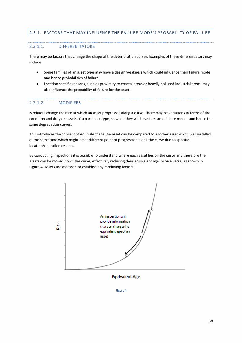
38

2.3.1. FACTORS THAT MAY INFLUENCE THE FAILURE MODE’S PROBABILITY OF FAILURE

2.3.1.1. DIFFERENTIATORS

There may be factors that change the shape of the deterioration curves. Examples of these differentiators may

include:

Some families of an asset type may have a design weakness which could influence their failure mode

and hence probabilities of failure

Location specific reasons, such as proximity to coastal areas or heavily polluted industrial areas, may

also influence the probability of failure for the asset.

2.3.1.2. MODIFIERS

Modifiers change the rate at which an asset progresses along a curve. There may be variations in terms of the

condition and duty on assets of a particular type, so while they will have the same failure modes and hence the

same degradation curves.

This introduces the concept of equivalent age. An asset can be compared to another asset which was installed

at the same time which might be at different point of progression along the curve due to specific

location/operation reasons.

By conducting inspections it is possible to understand where each asset lies on the curve and therefore the

assets can be moved down the curve, effectively reducing their equivalent age, or vice versa, as shown in

Figure 4. Assets are assessed to establish any modifying factors.

Figure 4

39

2.3.2. MAPPING END OF LIFE MODIFIER TO PROBABILITY OF FAILURE

End of life (EOL) can be defined as when the condition related probability of failure becomes unacceptable. It

may be difficult to define unacceptable PoF, and indeed it may vary from asset to asset. For every individual

asset we determine an EOL Modifier. The EOL Modifier will then need to be translated into an EOL probability

of failure.

The method for translating the EOL Modifier into a probability depends on the asset type. Asset types may

need their EOL Modifier translated into an Equivalent Age. The Equivalent Age can then be used to determine

probability of failure for a specific end of life failure mode.

The method described here generates an expected end of life modifier function, which is used to map

between the EOL modifier and an Equivalent Age. The following paragraph describes how this mapping

function can be produced.

The mapping function cannot be generated using historical data points, because the data is right censored due

to the fact that many assets have not completed a whole lifecycle. We therefore need to apply judgement

about how the health of an asset is expected to deteriorate through its life. The end of life modifier is then

mapped to an equivalent age, which is used by FMEA to determine the conditional probability of failure for the

corresponding end of life failure mode.

2.3.3. CALCULATING PROBABILITY OF FAILURE

As described above the probability of failure curve is based in terms of two data points that correspond to the

ages at which specific proportions of the asset’s population is expected to have failed. Using these data points

we can construct a cumulative distribution function F(t).

In order to calculate the end of life probability of failure associated with a given asset, the asset will need to be

assigned an end of life modifier. This end of life modifier is derived from values such as age, duty and condition

information where it is available. In the absence of any condition information age is used. The service

experience of assets of the same design as well as forensic examination of decommissioned assets may also be

taken into account when assigning an end of life modifier. Using the end of life modifier we can then

determine an asset’s equivalent age and then map onto a specific point on the probability of failure curve.

Specific calculations on determining the End of Life Modifiers are found in the appendices to this methodology.

2.3.4. FORECASTING PROBABILITY OF FAILURE

We estimate future probability of failure by following the appropriate failure curve. Depending on the type of

failure mode the current position on the failure curve is identified using either age, equivalent age or last

intervention date. The forecast is determined by following this curve along usually at the rate of one year per

year. Figure 5 illustrates the probability of failure for an asset highlighting the probability of failure at an

equivalent age of 80.

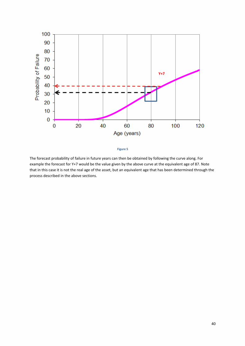
40

Figure 5

The forecast probability of failure in future years can then be obtained by following the curve along. For

example the forecast for Y+7 would be the value given by the above curve at the equivalent age of 87. Note

that in this case it is not the real age of the asset, but an equivalent age that has been determined through the

process described in the above sections.

Y+7

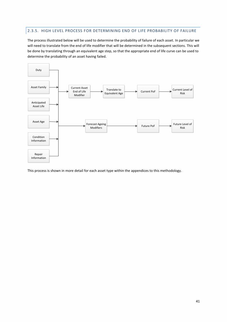
41

2.3.5. HIGH LEVEL PROCESS FOR DETERMINING END OF LIFE PROBABILITY OF FAILURE

The process illustrated below will be used to determine the probability of failure of each asset. In particular we

will need to translate from the end of life modifier that will be determined in the subsequent sections. This will

be done by translating through an equivalent age step, so that the appropriate end of life curve can be used to

determine the probability of an asset having failed.

This process is shown in more detail for each asset type within the appendices to this methodology.

Duty

Asset Family

Anticipated Asset Life

Asset Age

Condition Information

Repair Information

Current Asset End of Life Modifier

Forecast Ageing Modifiers

Translate to Equivalent Age

Current PoFCurrent Level of

Risk

Future PoFFuture Level of

Risk

42

3. CONSEQUENCE OF FAILURE

FMECA takes the principles of FMEA and incorporates criticality factors.

The consequences of the failure may fall into four categories:

Consequence Description

Safety Impact of direct harm to public/personnel as a result of failure mode

Environment Impact of failure mode taking into account the sensitivity of the geographical area local to the asset

Financial Cost of the intervention needed to address and resolve the failure

System The impact on the network of the failure and any subsequent intervention required

These categories reflect the impact of the various failure modes which are specific to the asset and the consequences

are consistent for each class of failure mode. The impact of the various failure modes will vary depending on the type of

failure. For example, for less disruptive failure modes there may be no impact from a safety perspective.

Safety and environmental consequence are specific to the asset and also to its physical location.

In considering the safety and environement concequences, the concept of exposure is needed. Exposure is based upon

the asset’s location, i.e. its proximity to a location where it has the potential to cause harm (whether to people or the

environment).

Each consequence will be monetised and the price base for consequence of failure will be agreed with Ofgem.

Each TO states clearly which failure modes have been included in the analysis and explains why the chosen failure

modes are considered appropriate for the analysis, as detailed in the technical appendices to this methodology. The

appendices also detail how the Probability of Failure (PoF) has been determined and how modifiers have been applied

to determine the asset PoF.

BS EN60812 disaggregates systems into their component parts and assesses the probability of functional failures of each

component and the consequences of such functional failures, then aggregates these quantities to obtain an estimate of

the overall risk of the system. A failure mode is clearly immaterial if the cost of the analysis of the functional failure of a

component is much greater than value of the risk represented by the functional failure of that component, because

either the probability of functional failure of a component or the consequence of failure of a component is insufficiently

large.

Evidential and supporting data, suitable for FMECA analysis is usually imperfect. Some possible effects and

consequences might be material, but have not yet occurred. Similarly, accurate data may not have been captured for

failures, even though the effects and consequences have occurred. Effective application of FMECA therefore requires

engineering judgement, both to envision material consequences that have not yet occurred and to estimate values

which have not been measured and / or recorded and which cannot be reliably calculated from first principles.

There is a further requirement in the Direction to enable the identification of all material factors contributing to real or

apparent performance against targets.

A non-exhaustive list of these factors is identified in Paragraph 32 of the Direction. In practice, the effect of any of these

factors will be a modification to one or more inputs to the methodology. By definition, any factor which does not result

in a modification to one or more of the inputs does not contribute to real or apparent performance against targets as

measured by this methodology.

For factors that do modify one or more inputs to the methodology, the methodology can be re-run incorporating these

input changes and the outcomes compared with the outcomes produced before the changes are applied. Hence not

only can factors be identified but also their relative materiality can be determined.

43

Therefore if a TO (or Ofgem) suspects that a factor (e.g. data revisions) or change in external environment (business,

legal, site or situation) will contribute to real or apparent performance against targets, then the following tests can be

made:

1. Check what impact the factor has on existing inputs to the methodology – if the impact is zero then the factor

has been positively classified as non-material

2. If impact is non-zero then re-run the methodology with changed inputs and compare outputs with equivalent

outputs with the un-changed inputs – The variation of output can be compared with the variations produced

by other factors and ranked in terms of relative materiality

It is the aim of this section to provide quantified view in the terms of a monetised consequence.

In taking the below detailed approach it is intended that the quantification forms an approximation to how this may

play out in the real world. In this case an approximation is of much greater value, due to its simplified nature and the

ease of comparison and benchmark. All quantities used will be externally verifiable and benchmarked.

The monetisation does not correspond to the actual costs that will be incurred. The data used in the models attempts to

approach the correct orders of magnitude to avoid confusion it does not however, guarantee this and can only be

treated as abstract.

44

3.1. SYSTEM CONSEQUENCE

The system consequence of a failure mode of an asset is a measure of the assets importance in terms of its function to

the transmission system and the disruption to that function caused by the failure. It is measured in terms of certain

system related costs associated with system consequences incurred by the industry electricity sector if that asset were

to experience a failure. These system costs incurred due to an asset failure can be divided into two categories, customer

costs and System Operator costs. Regardless of who initially pays these costs they are ultimately born by electricity

consumers. Customer costs are incurred as a result of the disconnection of customers supplied directly or indirectly (via

a distribution network) connected by the transmission system. The cost for demand disconnections are expressed as

the economic value that the user assigns to that lost load. In the case of generators being disconnected from the

network there is a mechanism of direct compensation payments from the System Operator. The second category of

costs are those that the System Operator incurs in undertaking corrective and preventative measures to secure the

system after asset failures have occurred. These include generator constraint payments, response and reserve costs and

auxiliary services costs.

Unlike the environmental, financial and safety consequences of asset failures, the existence and scale of network risk

due to asset failures is dependent on the functional role that the failed asset plays in the transmission system. The

transmission system is designed with a degree of resilience that seeks to ensure the impact of asset faults is contained

within acceptable limits. It is the National Electricity Transmission System Security and Quality of Supply Standard (NETS

SQSS) that mandates a certain level of resilience that the design and operation of the transmission system must meet

when faced with a range of scenarios and events. It is a license obligation of Transmission Owners that their networks

comply with the NETS SQSS.

A range of negative system consequences (unacceptable overloading of primary transmission equipment, unacceptable

voltage conditions or system instability) must be avoided for ‘defined secured events’ under certain network conditions.

The required resilience is not absolute nor is it uniform across the network. The philosophy behind the NETS SQSS is

that lower severity consequences are to be accepted for relatively high probability (and therefore high frequency) faults

while more severe consequences are only to be accepted for lower probability events. Figure 6 represents this

philosophy.

This approach is further influenced by other considerations such as the geographical location of the assets in question

i.e. which Transmission Owner License Area they are in, and for what timescales the network is being assessed (near

term operational timescales vs. long term planning timescales). The level of resilience required also varies depending on

the function of the part of the network in question. Parts of the network which connect demand, generation or make up

part of the Main Interconnected Transmission System (MITS) all have distinct design requirements dependent upon

their importance to the Transmission System and the total economic value of all the customers they supply.

45

Allowed

Not Allowed

Severity of

Consequence

Probability of

Fault

Figure 6

Events that the NETS SQSS requires a degree of resilience against are described as ‘secured events’. These are events

that occur with sufficient frequency that it is economic to invest in transmission infrastructure to prevent certain

consequences when such events occur on the system. Secured events include faults on equipment and these events

range from single transmission circuit faults (highest frequency) to circuit breaker faults (lowest frequency). When an

asset fault occurs that results in the loss of only a single transmission circuit in an otherwise intact network, almost no

customer losses are permitted and all system parameters must stay within limits without the SO taking immediate post-

fault actions. While in the case of circuit breaker faults the NETS SQSS only requires that the system is planned such that

customer losses are contained to the level necessary to ensure the system frequency stays within statutory limits to

avoid total system collapse.

The key assumption that underpins this variation in permitted consequences of faults is that most faults are weather

related and that faults caused by the condition of the asset are rare. This can be seen in that faults on overhead lines

(often affected by wind and lightning) are relatively frequent events (≈20% probability per 100 km 400 kV circuit per

annum) while switchgear faults are relatively less frequent (≈2% probability per 2-ended 400 kV circuit per annum).

Another key assumption in the design of the SQSS is that faults are relatively short in duration. A vast majority of circuits

have a post-fault rating that is time limited to 24 hours, it is expected that faults will be resolved within this time so that

this rating will not be exceeded.

Asset failures driven by asset condition do not conform to these key assumptions, they occur in assets regardless of

their exposure to the elements and they can significantly exceed 24 hours in duration. The system therefore cannot be

assumed to be designed to be resilient against even a single asset failure. Even if system resilience is sufficient to avoid

an immediate customer or operator cost no asset fault or failure that requires offline intervention can be said to be free

from a risk cost. At the very least the unavailability of the asset reduces system resilience to further events and

therefore increases exposure to future costs.

46

3.1.1. QUANTIFYING THE SYSTEM RISK DUE TO ASSET FAULTS AND FAILURES

Fundamentally the transmission system performs three functions. It receives power from generators, transports power

where it is needed and delivers it to consumers. The system risk cost of a fault or failure can be quantified by combining

the following costs:

1. The economic value assigned to load not supplied to consumers. Commonly described as Value of Lost Load

(VOLL) in units of £/MWh

2. The cost of compensating generators disconnected from the transmission system, based on the market cost of

generation (£/MWh), the size of the generator (MW) and the expected duration of disconnection (hours)

3. The cost of paying for other generators to replace the power lost from disconnected generation based on the

market cost of replacement generation (£/MWh) and number of megawatt hours that require replacement

4. The increased cost in transporting power across the wider transmission network. This is comprised of:

a. Constraint payments to generators due to insufficient capacity in part of the transmission system. This

comprises the costs to constrain off generation affected by the insufficient capacity and the cost to

constrain on generation to replace it. If there is insufficient replacement generation capacity, costs

will include demand reduction.

b. Payments to generators to provide auxiliary services which ensure system security and quality of

supply e.g. the provision of reactive power.

The applicability and size of these cost sources are dependent upon the role of the failed asset in the system. Some

assets are solely for the connection of generation or demand, while others will provide multiple functions.

The methodology for calculating these potential costs is split into three parts:

1. A customer disconnection methodology, incorporating the cost of disconnecting generation, total consumer

demand and vital infrastructure sites (1, 2 and 3 above)

2. A boundary transfer methodology that estimates potential generator constraint payments (4a)

3. A reactive compensation methodology that estimates the cost of procuring reactive power to replace that

provided by faulted assets (4b)

Each of these methodologies will be described in turn in the following three sections. All three share a common

structure that can be expressed by Equation 4.

𝑐𝑜𝑠𝑡 𝑜𝑓 𝑐𝑜𝑛𝑠𝑒𝑞𝑢𝑒𝑛𝑐𝑒 = 𝑝𝑟𝑜𝑏𝑎𝑏𝑖𝑙𝑖𝑡𝑦 𝑥 𝑑𝑢𝑟𝑎𝑡𝑖𝑜𝑛 𝑥 𝑠𝑖𝑧𝑒 𝑥 𝑐𝑜𝑠𝑡 𝑝𝑒𝑟 𝑢𝑛𝑖𝑡

Equation 4

The total system consequence cost of a failure mode of an asset will be the sum of the consequence costs that come

from the following three costs.

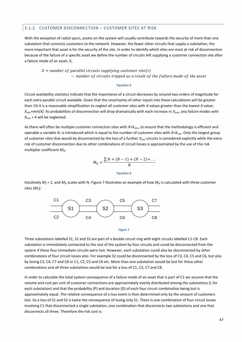
47

3.1.2. CUSTOMER DISCONNECTION – CUSTOMER SITES AT RISK

With the exception of radial spurs, assets on the system will usually contribute towards the security of more than one

substation that connects customers to the network. However, the fewer other circuits that supply a substation, the

more important that asset is for the security of the site. In order to identify which sites are most at risk of disconnection

because of the failure of a specific asset we define the number of circuits left supplying a customer connection site after

a failure mode of an asset, X;

𝑋 = 𝑛𝑢𝑚𝑏𝑒𝑟 𝑜𝑓 𝑝𝑎𝑟𝑎𝑙𝑙𝑒𝑙 𝑐𝑖𝑟𝑐𝑢𝑖𝑡𝑠 𝑠𝑢𝑝𝑝𝑙𝑦𝑖𝑛𝑔 𝑐𝑢𝑠𝑡𝑜𝑚𝑒𝑟 𝑠𝑖𝑡𝑒(𝑠)

− 𝑛𝑢𝑚𝑏𝑒𝑟 𝑜𝑓 𝑐𝑖𝑟𝑐𝑢𝑖𝑡𝑠 𝑡𝑟𝑖𝑝𝑝𝑒𝑑 𝑎𝑠 𝑎 𝑟𝑒𝑠𝑢𝑙𝑡 𝑜𝑓 𝑡ℎ𝑒 𝑓𝑎𝑖𝑙𝑢𝑟𝑒 𝑚𝑜𝑑𝑒 𝑜𝑓 𝑡ℎ𝑒 𝑎𝑠𝑠𝑒𝑡

Equation 5

Circuit availability statistics indicate that the importance of a circuit decreases by around two orders of magnitude for

each extra parallel circuit available. Given that the uncertainty of other inputs into these calculations will be greater

than 1% it is a reasonable simplification to neglect all customer sites with X values greater than the lowest X value;

Xmin=min(X). As probabilities of disconnection will drop dramatically with each increase in Xmin, any failure modes with

Xmin > 4 will be neglected.

As there will often be multiple customer connection sites with X=Xmin, to ensure that the methodology is efficient and

operable a variable N, is introduced which is equal to the number of customer sites with X=Xmin. Only the largest group

of customer sites that would be disconnected by the loss of a further Xmin circuits is considered explicitly while the extra

risk of customer disconnection due to other combinations of circuit losses is approximated by the use of the risk

multiplier coefficient MN:

𝑀𝑁 =∑𝑁 + (𝑁 − 1) + (𝑁 − 2)+ . . .

𝑁

Equation 6

Intuitively M1 = 1, and MN scales with N. Figure 7 illustrates an example of how MN is calculated with three customer

sites (M3):

S1 S3S2

C1

C2

C3

C4

C5

C6

C7

C8

Figure 7

Three substations labelled S1, S2 and S3 are part of a double circuit ring with eight circuits labelled C1-C8. Each

substation is immediately connected to the rest of the system by four circuits and could be disconnected from the

system if these four immediate circuits were lost. However, each substation could also be disconnected by other

combinations of four circuit losses also. For example S2 could be disconnected by the loss of C3, C4, C5 and C6, but also

by losing C3, C4, C7 and C8 or C1, C2, C5 and C6 etc. More than one substation would be lost for these other

combinations and all three substations would be lost for a loss of C1, C2, C7 and C8.

In order to calculate the total system consequence of a failure mode of an asset that is part of C1 we assume that the

volume and cost per unit of customer connections are approximately evenly distributed among the substations (L for

each substation) and that the probability (P) and duration (D) of each four circuit combination being lost is

approximately equal. The relative consequence of a loss event is then determined only by the amount of customers

lost. So a loss of S1 and S2 is twice the consequence of losing only S1. There is one combination of four circuit losses

involving C1 that disconnected a single substation, one combination that disconnects two substations and one that

disconnects all three. Therefore the risk cost is:

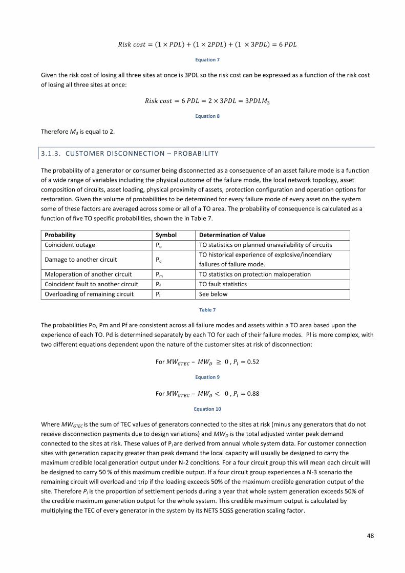
48

𝑅𝑖𝑠𝑘 𝑐𝑜𝑠𝑡 = (1 × 𝑃𝐷𝐿) + (1 × 2𝑃𝐷𝐿) + (1 × 3𝑃𝐷𝐿) = 6 𝑃𝐷𝐿

Equation 7

Given the risk cost of losing all three sites at once is 3PDL so the risk cost can be expressed as a function of the risk cost

of losing all three sites at once:

𝑅𝑖𝑠𝑘 𝑐𝑜𝑠𝑡 = 6 𝑃𝐷𝐿 = 2 × 3𝑃𝐷𝐿 = 3𝑃𝐷𝐿𝑀3

Equation 8

Therefore M3 is equal to 2.

3.1.3. CUSTOMER DISCONNECTION – PROBABILITY

The probability of a generator or consumer being disconnected as a consequence of an asset failure mode is a function

of a wide range of variables including the physical outcome of the failure mode, the local network topology, asset

composition of circuits, asset loading, physical proximity of assets, protection configuration and operation options for

restoration. Given the volume of probabilities to be determined for every failure mode of every asset on the system

some of these factors are averaged across some or all of a TO area. The probability of consequence is calculated as a

function of five TO specific probabilities, shown the in Table 7.

Probability Symbol Determination of Value

Coincident outage Po TO statistics on planned unavailability of circuits

Damage to another circuit Pd TO historical experience of explosive/incendiary

failures of failure mode.

Maloperation of another circuit Pm TO statistics on protection maloperation

Coincident fault to another circuit Pf TO fault statistics

Overloading of remaining circuit Pl See below

Table 7

The probabilities Po, Pm and Pf are consistent across all failure modes and assets within a TO area based upon the

experience of each TO. Pd is determined separately by each TO for each of their failure modes. Pl is more complex, with

two different equations dependent upon the nature of the customer sites at risk of disconnection:

For 𝑀𝑊𝐺𝑇𝐸𝐶 – 𝑀𝑊𝐷 ≥ 0 , 𝑃𝑙 = 0.52

Equation 9

For 𝑀𝑊𝐺𝑇𝐸𝐶 – 𝑀𝑊𝐷 < 0 , 𝑃𝑙 = 0.88

Equation 10

Where MWGTEC is the sum of TEC values of generators connected to the sites at risk (minus any generators that do not

receive disconnection payments due to design variations) and MWD is the total adjusted winter peak demand

connected to the sites at risk. These values of Pl are derived from annual whole system data. For customer connection

sites with generation capacity greater than peak demand the local capacity will usually be designed to carry the

maximum credible local generation output under N-2 conditions. For a four circuit group this will mean each circuit will

be designed to carry 50 % of this maximum credible output. If a four circuit group experiences a N-3 scenario the

remaining circuit will overload and trip if the loading exceeds 50% of the maximum credible generation output of the

site. Therefore Pl is the proportion of settlement periods during a year that whole system generation exceeds 50% of

the credible maximum generation output for the whole system. This credible maximum output is calculated by

multiplying the TEC of every generator in the system by its NETS SQSS generation scaling factor.

49

For customer sites with peak demand greater than generation capacity the local capacity will be designed to carry

access period peak (85% of winter peak demand is the system wide average) under N-2 conditions. This requires each

circuit to be designed to carry 50% of access period demand, or on average 42.5% of winter peak demand of the site. If

a four circuit group experiences a N-3 scenario the remaining circuit will overload and trip if the loading exceeds 42.5%

of the maximum credible generation output of the site. Therefore this value of Pl represents the proportion of

settlement periods during the year that total system demand is in excess of 42.5% of total system winter peak demand.

The probabilities in Table 7 can be combined to create a probability tree for each value of Xmin between 0 and 4. Below

are the resulting equations for Poc, the probability of disconnection.

For Xmin =0, Poc = 1

Equation 11

For Xmin = 1, Poc = 1 - NoNdNmNf

Equation 12

For Xmin = 2, Poc = Pd2 + 2PdNdPo + 2PdNdNoPm + 2PdNdNoNmPf + Nd

2PoPm + Nd

2PoNmPf + Nd

2NoPmPf + Nd

2NoNmPf

2

Equation 13

For Xmin = 3, Poc = Pd2Po + Pd

2NoPm + Pd

2NoNmPf + Pd

2NoNmNfPl + 2PdNdPoPm + 2PdNdPoNmPf + 2PdNdPoNmNfPl + 2PdNdNoPmPf +

2PdNdNoPmNfPl + 2PdNdNoNmPf2 + 4PdNdNoNmPfNfPl + Nd

2PoPmPf + Nd

2PoPmNfPl + Nd

2PoNmPf

2 + 2Nd

2PoNmPfNfPl + Nd

2NoPmPf

2 +

2Nd2NoPmPfNfPl + Nd

2NoNmPf

3 + 3Nd

2NoNmPf

2NfPl

Equation 14

Where No, Nd, Nm, Nf and Nl are the probabilities of no outage, no damage, no maloperation, no coincident faults and no

overloading respectively.

The derivation method of the above probability equations can be followed in Figure 8, the probability tree diagram for

the most complex of the four cases, Xmin = 3.

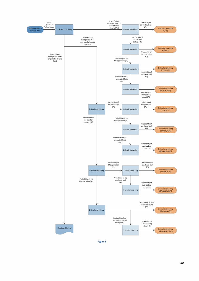
50

Initial pre-failure network state

Asset Experience

Failure Mode

3 circuits remaining

Probability of parallel outage

(Po)0 circuits remaining

(Pd2Po)

1 circuit remaining

Asset Failure damages asset on

two parallel circuits (Pd

2)

Probability of no parallel outage (No)

Probability of Maloperation

(Pm)

1 circuit remaining0 circuits remaining

(Pd2NoPm)

1 circuit remaining

Probability of no Maloperation (Nm)

1 circuit remaining

Probability of unrelated fault

(Pf)

0 circuits remaining(Pd

2NoNmPf)

Probability of no unrelated fault

(Nf)

Probability of overloading circuit (Pl)

0 circuits remaining(Pd

2NoNmNfPl)


Asset Failure damages asset on one parallel circuit

(2PdNd)

1 circuit remaining


(Pm)0 circuits remaining

(2PdNdPoPm)


(Po)


(2PdNdPoNmPf)



(Pf)


(Nf)


(2PdNdPoNmNfPl)





(Pm)

1 circuit remaining


(Pf)


(Nf)

1 circuit remaining

0 circuits remaining(2PdNdNoPmPf)


0 circuits remaining(2PdNdNoPmNfPl)


2 circuits remaining0 circuits remaining

(2PdNdNoNmPf2)

Probability of two unrelated faults

(Pf2)

Probability of no second unrelated

fault (2PfNf)

1 circuit remaining0 circuits remaining(4PdNdNoNmPfNfPl)


Asset Failure damages no assets on parallel circuits

(Nd2)

Continued Below

Figure 8

51



(Po)2 circuits remaining


(Pm)1 circuit remaining

0 circuits remaining(Nd

2PoPmPf)


(Pf)



(Nd2PoPmNfPl)

Probability of no unrelated fault (Nf)


Probability of no maloperation (Nm)

0 circuits remaining(Nd

2PoNmPf2)


(Pf2)


fault (2PfNf)


(2Nd2PoNmPfNfPl)





(Pm)


(Nd2NoPmPf

2)


(Pf2)


fault (2PfNf)


(2Nd2NoPmPfNfPl)


Probability of no maloperation (Nm)


(Nd2NoNmPf

3)

Probability of three unrelated

faults (Pf2)


(3PfPfNf)

1 circuit remaining0 circuits remaining(3Nd

2NoNmPf2NfPl)


Continued

Figure 9

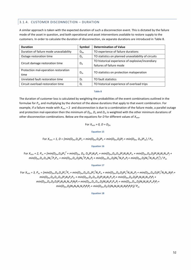
52

3.1.4. CUSTOMER DISCONNECTION – DURATION

A similar approach is taken with the expected duration of such a disconnection event. This is dictated by the failure

mode of the asset in question, and both operational and asset interventions available to restore supply to the

customers. In order to calculate the duration of disconnection, six separate durations are introduced in Table 8.

Duration Symbol Determination of Value

Duration of failure mode unavailability Dfm TO experience of failure durations

Outage restoration time Do TO statistics on planned unavailability of circuits

Circuit damage restoration time Dd TO historical experience of explosive/incendiary

failures of failure mode

Protection mal-operation restoration

time Dm TO statistics on protection maloperation

Unrelated fault restoration time Df TO fault statistics

Circuit overload restoration time Dl TO historical experience of overload trips

Table 8

The duration of customer loss is calculated by weighting the probabilities of the event combinations outlined in the

formulae for Poc and multiplying by the shortest of the above durations that apply to that event combination. For

example, if a failure mode with Xmin = 2 and disconnection is due to a combination of the failure mode, a parallel outage

and protection mal-operation then the minimum of Dfm, Do and Dm is weighted with the other minimum durations of

other disconnection combinations. Below are the equations for D for different values of Xmin.

For Xmin = 0, D = Dfm

Equation 15

For Xmin = 1, D = [min(Dfm,Do)Po + min(Dfm,Dd)Pd + min(Dfm,Df)Pf + min(Dfm, Dm)Pm] / Poc

Equation 16

For Xmin = 2, Poc = [min(Dfm,Dd)Pd2 + min(Dfm, Dd, Do)PdNdPo + min(Dfm,Dd,Dm)PdNdNoPm + min(Dfm,Dd,Df)PdNdNoNmPf +

min(Dfm,Do,Dm)Nd2PoPm + min(Dfm,Do,Df)Nd

2PoNmPf + min(Dfm,Dm,Df)Nd

2NoPmPf + min(Dfm,Df)Nd

2NoNmPf

2] / Poc

Equation 17

For Xmin = 3, Poc = [min(Dfm,Dd,Do)Pd2Po + min(Dfm,Dd,Dm)Pd

2NoPm + min(Dfm,Dd,Df)Pd

2NoNmPf + min(Dfm,Dd,Dl)Pd

2NoNmNfPl +

min(Dfm,Dd,Do,Dm)PdNdPoPm + min(Dfm,Dd,Dm,Df)PdNdNoPmPf + min(Dfm,Dd,Df)PdNdNoNmPfPf +

min(Dfm,Dd,Df,Dl)PdNdNoNmPfNfPl + min(Dfm,Do,Dm,Df)NdNdPoPmPf + min(Dfm,Dm,Df)NdNdNoPmPfPf +

min(Dfm,Df)NdNdNoNoPfPfPf + min(Dfm,Df,Dl)NdNdNoNoNfPfPfPl]/ Poc

Equation 18

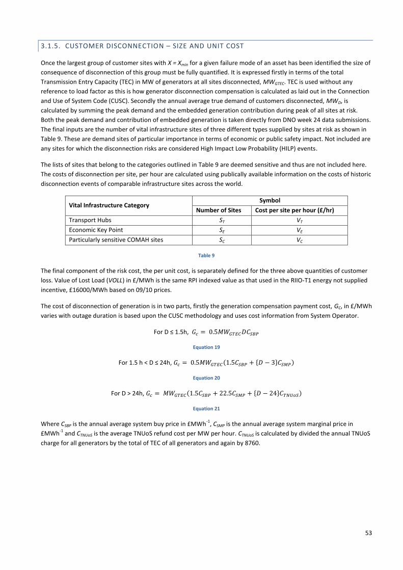
53

3.1.5. CUSTOMER DISCONNECTION – SIZE AND UNIT COST

Once the largest group of customer sites with X = Xmin for a given failure mode of an asset has been identified the size of

consequence of disconnection of this group must be fully quantified. It is expressed firstly in terms of the total

Transmission Entry Capacity (TEC) in MW of generators at all sites disconnected, MWGTEC. TEC is used without any

reference to load factor as this is how generator disconnection compensation is calculated as laid out in the Connection

and Use of System Code (CUSC). Secondly the annual average true demand of customers disconnected, MWD, is

calculated by summing the peak demand and the embedded generation contribution during peak of all sites at risk.

Both the peak demand and contribution of embedded generation is taken directly from DNO week 24 data submissions.

The final inputs are the number of vital infrastructure sites of three different types supplied by sites at risk as shown in

Table 9. These are demand sites of particular importance in terms of economic or public safety impact. Not included are

any sites for which the disconnection risks are considered High Impact Low Probability (HILP) events.

The lists of sites that belong to the categories outlined in Table 9 are deemed sensitive and thus are not included here.

The costs of disconnection per site, per hour are calculated using publically available information on the costs of historic

disconnection events of comparable infrastructure sites across the world.

Vital Infrastructure Category Symbol

Number of Sites Cost per site per hour (£/hr)

Transport Hubs ST VT

Economic Key Point SE VE

Particularly sensitive COMAH sites SC VC

Table 9

The final component of the risk cost, the per unit cost, is separately defined for the three above quantities of customer

loss. Value of Lost Load (VOLL) in £/MWh is the same RPI indexed value as that used in the RIIO-T1 energy not supplied

incentive, £16000/MWh based on 09/10 prices.

The cost of disconnection of generation is in two parts, firstly the generation compensation payment cost, GC, in £/MWh

varies with outage duration is based upon the CUSC methodology and uses cost information from System Operator.

For D ≤ 1.5h, 𝐺𝑐 = 0.5𝑀𝑊𝐺𝑇𝐸𝐶𝐷𝐶𝑆𝐵𝑃

Equation 19

For 1.5 h < D ≤ 24h, 𝐺𝑐 = 0.5𝑀𝑊𝐺𝑇𝐸𝐶(1.5𝐶𝑆𝐵𝑃 + {𝐷 − 3}𝐶𝑆𝑀𝑃)

Equation 20

For D > 24h, 𝐺𝑐 = 𝑀𝑊𝐺𝑇𝐸𝐶(1.5𝐶𝑆𝐵𝑃 + 22.5𝐶𝑆𝑀𝑃 + {𝐷 − 24}𝐶𝑇𝑁𝑈𝑜𝑆)

Equation 21

Where CSBP is the annual average system buy price in £MWh-1

, CSMP is the annual average system marginal price in

£MWh-1

and CTNUoS is the average TNUoS refund cost per MW per hour. CTNUoS is calculated by divided the annual TNUoS

charge for all generators by the total of TEC of all generators and again by 8760.

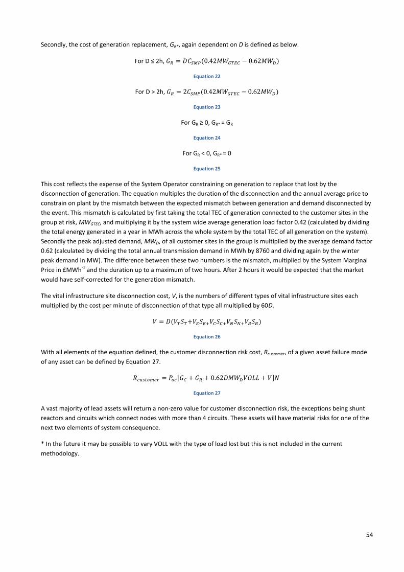
54

Secondly, the cost of generation replacement, GR*, again dependent on D is defined as below.

For D ≤ 2h, 𝐺𝑅 = 𝐷𝐶𝑆𝑀𝑃(0.42𝑀𝑊𝐺𝑇𝐸𝐶 − 0.62𝑀𝑊𝐷)

Equation 22

For D > 2h, 𝐺𝑅 = 2𝐶𝑆𝑀𝑃(0.42𝑀𝑊𝐺𝑇𝐸𝐶 − 0.62𝑀𝑊𝐷)

Equation 23

For GR ≥ 0, GR* = GR

Equation 24

For GR < 0, GR* = 0

Equation 25

This cost reflects the expense of the System Operator constraining on generation to replace that lost by the

disconnection of generation. The equation multiples the duration of the disconnection and the annual average price to

constrain on plant by the mismatch between the expected mismatch between generation and demand disconnected by

the event. This mismatch is calculated by first taking the total TEC of generation connected to the customer sites in the

group at risk, MWGTEC, and multiplying it by the system wide average generation load factor 0.42 (calculated by dividing

the total energy generated in a year in MWh across the whole system by the total TEC of all generation on the system).

Secondly the peak adjusted demand, MWD, of all customer sites in the group is multiplied by the average demand factor

0.62 (calculated by dividing the total annual transmission demand in MWh by 8760 and dividing again by the winter

peak demand in MW). The difference between these two numbers is the mismatch, multiplied by the System Marginal

Price in £MWh-1

and the duration up to a maximum of two hours. After 2 hours it would be expected that the market

would have self-corrected for the generation mismatch.

The vital infrastructure site disconnection cost, V, is the numbers of different types of vital infrastructure sites each

multiplied by the cost per minute of disconnection of that type all multiplied by 60D.

𝑉 = 𝐷(𝑉𝑇𝑆𝑇+𝑉𝐸𝑆𝐸+𝑉𝐶𝑆𝐶+𝑉𝑁𝑆𝑁+𝑉𝐵𝑆𝐵)

Equation 26

With all elements of the equation defined, the customer disconnection risk cost, Rcustomer, of a given asset failure mode

of any asset can be defined by Equation 27.

𝑅𝑐𝑢𝑠𝑡𝑜𝑚𝑒𝑟 = 𝑃𝑜𝑐[𝐺𝐶 + 𝐺𝑅 + 0.62𝐷𝑀𝑊𝐷𝑉𝑂𝐿𝐿 + 𝑉]𝑁

Equation 27

A vast majority of lead assets will return a non-zero value for customer disconnection risk, the exceptions being shunt

reactors and circuits which connect nodes with more than 4 circuits. These assets will have material risks for one of the

next two elements of system consequence.

* In the future it may be possible to vary VOLL with the type of load lost but this is not included in the current

methodology.

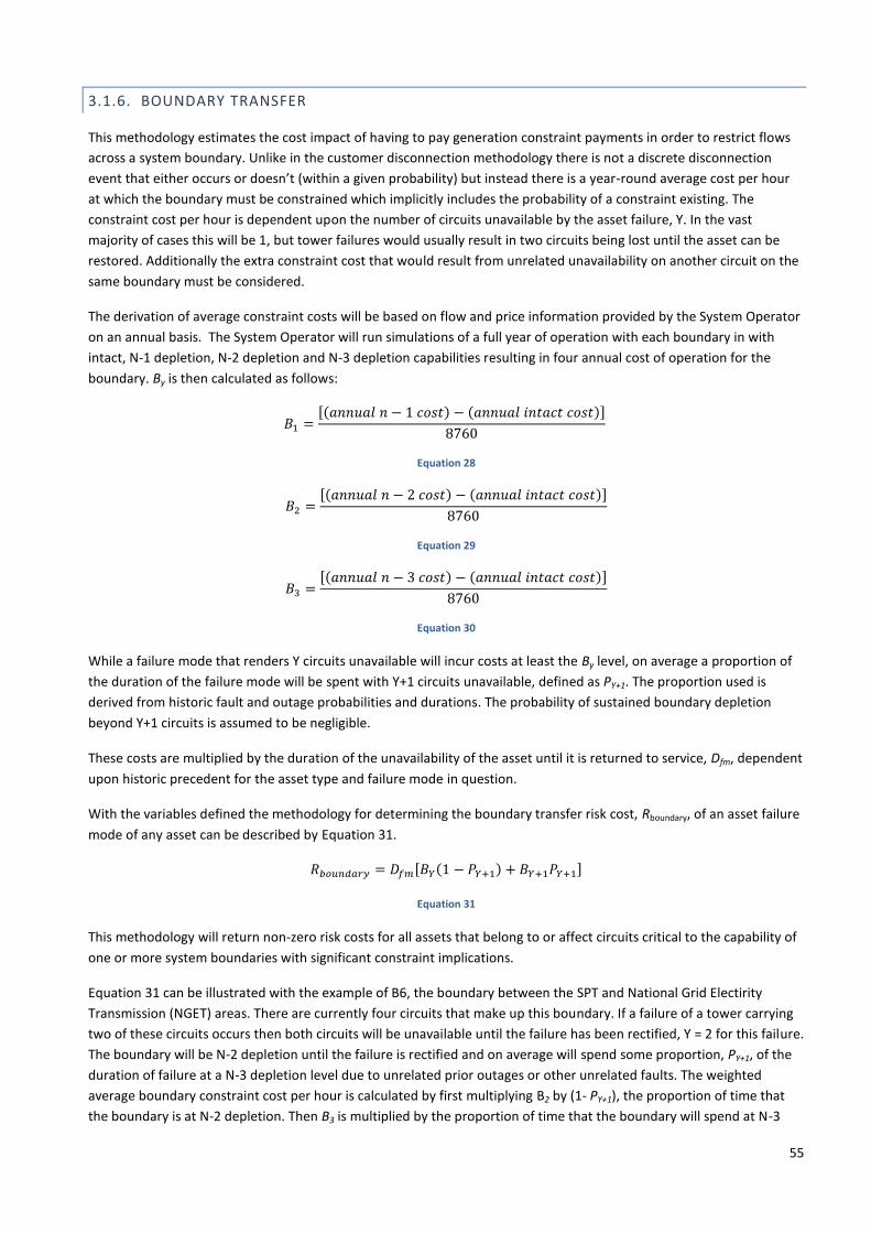
55

3.1.6. BOUNDARY TRANSFER

This methodology estimates the cost impact of having to pay generation constraint payments in order to restrict flows

across a system boundary. Unlike in the customer disconnection methodology there is not a discrete disconnection

event that either occurs or doesn’t (within a given probability) but instead there is a year-round average cost per hour

at which the boundary must be constrained which implicitly includes the probability of a constraint existing. The

constraint cost per hour is dependent upon the number of circuits unavailable by the asset failure, Y. In the vast

majority of cases this will be 1, but tower failures would usually result in two circuits being lost until the asset can be

restored. Additionally the extra constraint cost that would result from unrelated unavailability on another circuit on the

same boundary must be considered.

The derivation of average constraint costs will be based on flow and price information provided by the System Operator

on an annual basis. The System Operator will run simulations of a full year of operation with each boundary in with

intact, N-1 depletion, N-2 depletion and N-3 depletion capabilities resulting in four annual cost of operation for the

boundary. By is then calculated as follows:

𝐵1 =[(𝑎𝑛𝑛𝑢𝑎𝑙 𝑛 − 1 𝑐𝑜𝑠𝑡) − (𝑎𝑛𝑛𝑢𝑎𝑙 𝑖𝑛𝑡𝑎𝑐𝑡 𝑐𝑜𝑠𝑡)]

8760

Equation 28


8760

Equation 29


8760

Equation 30

While a failure mode that renders Y circuits unavailable will incur costs at least the By level, on average a proportion of

the duration of the failure mode will be spent with Y+1 circuits unavailable, defined as PY+1. The proportion used is

derived from historic fault and outage probabilities and durations. The probability of sustained boundary depletion

beyond Y+1 circuits is assumed to be negligible.

These costs are multiplied by the duration of the unavailability of the asset until it is returned to service, Dfm, dependent

upon historic precedent for the asset type and failure mode in question.

With the variables defined the methodology for determining the boundary transfer risk cost, Rboundary, of an asset failure

mode of any asset can be described by Equation 31.

𝑅𝑏𝑜𝑢𝑛𝑑𝑎𝑟𝑦 = 𝐷𝑓𝑚[𝐵𝑌(1 − 𝑃𝑌+1) + 𝐵𝑌+1𝑃𝑌+1]

Equation 31

This methodology will return non-zero risk costs for all assets that belong to or affect circuits critical to the capability of

one or more system boundaries with significant constraint implications.

Equation 31 can be illustrated with the example of B6, the boundary between the SPT and National Grid Electirity

Transmission (NGET) areas. There are currently four circuits that make up this boundary. If a failure of a tower carrying

two of these circuits occurs then both circuits will be unavailable until the failure has been rectified, Y = 2 for this failure.

The boundary will be N-2 depletion until the failure is rectified and on average will spend some proportion, PY+1, of the

duration of failure at a N-3 depletion level due to unrelated prior outages or other unrelated faults. The weighted

average boundary constraint cost per hour is calculated by first multiplying B2 by (1- PY+1), the proportion of time that

the boundary is at N-2 depletion. Then B3 is multiplied by the proportion of time that the boundary will spend at N-3

56

depletion, PY+1. These two products are added together. This average boundary cost per hour is then simply multiplied

by the average time taken to restore the circuits to service by repairing the failed tower, Dfm. This gives us the total

expected boundary constraint for the failure mode of the tower.

3.1.7. REACTIVE COMPENSATION

The third methodology calculates the cost impact of having reactive compensation unavailable due to a fault or failure

of such an asset. The purpose of reactive compensation is to produce or consume reactive power to aid control of

system voltage. When compensation equipment is unavailable this reactive power control is either procured from

generators instead or elements of the transmission system are de-energised, reducing system resilience. As a

simplification the cost impact of a fault or failure can be quantified as the volume of reactive power not supplied

multiplied by the cost per MVArh the SO must pay to buy the same service from generators. Therefore we have

Equation 31 to calculate the reactive compensation system risk cost, RRC, of an asset failure mode:

𝑅𝑅𝐶 = 𝑅𝐹𝐷𝑓𝑚𝑄𝐶𝑀𝑉𝐴𝑟ℎ

Equation 32

RF is the requirement factor of the compensation or the proportion of the year that the compensation is required. Dfm is

the duration of unavailability due to the asset failure mode. Q is the capacity of the asset in MVAr and CMVArh is the

average cost of procuring of MVAr from generation sources.

RF is assigned to each reactive compensation lead asset on the follow basis:

RF = 0.25 for a Summer only requirement

RF = 0.75 for a Summer, Spring and Autumn requirement

RF = 1 for year round requirement

CMVArh will be calculated by taking an annual sum of all costs of generators to absorb MVArs including BM actions to

bring plant into service and constrain others as well as the cost of providing the reactive absorption itself. This sum is

divided by the total number of MVArhs that were absorbed by generators over the year.

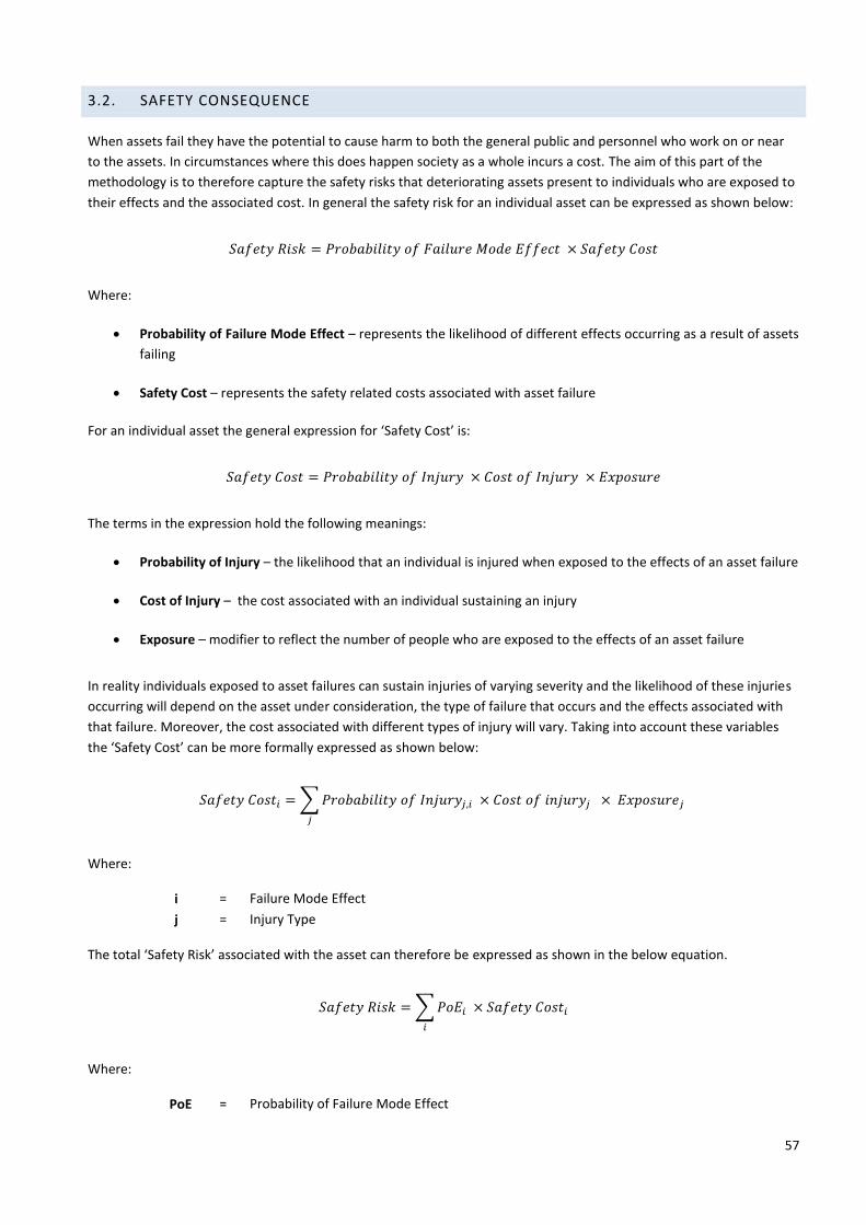
57

3.2. SAFETY CONSEQUENCE

When assets fail they have the potential to cause harm to both the general public and personnel who work on or near

to the assets. In circumstances where this does happen society as a whole incurs a cost. The aim of this part of the

methodology is to therefore capture the safety risks that deteriorating assets present to individuals who are exposed to

their effects and the associated cost. In general the safety risk for an individual asset can be expressed as shown below:

𝑆𝑎𝑓𝑒𝑡𝑦 𝑅𝑖𝑠𝑘 = 𝑃𝑟𝑜𝑏𝑎𝑏𝑖𝑙𝑖𝑡𝑦 𝑜𝑓 𝐹𝑎𝑖𝑙𝑢𝑟𝑒 𝑀𝑜𝑑𝑒 𝐸𝑓𝑓𝑒𝑐𝑡 × 𝑆𝑎𝑓𝑒𝑡𝑦 𝐶𝑜𝑠𝑡

Where:

Probability of Failure Mode Effect – represents the likelihood of different effects occurring as a result of assets

failing

Safety Cost – represents the safety related costs associated with asset failure

For an individual asset the general expression for ‘Safety Cost’ is:

𝑆𝑎𝑓𝑒𝑡𝑦 𝐶𝑜𝑠𝑡 = 𝑃𝑟𝑜𝑏𝑎𝑏𝑖𝑙𝑖𝑡𝑦 𝑜𝑓 𝐼𝑛𝑗𝑢𝑟𝑦 × 𝐶𝑜𝑠𝑡 𝑜𝑓 𝐼𝑛𝑗𝑢𝑟𝑦 × 𝐸𝑥𝑝𝑜𝑠𝑢𝑟𝑒

The terms in the expression hold the following meanings:

Probability of Injury – the likelihood that an individual is injured when exposed to the effects of an asset failure

Cost of Injury – the cost associated with an individual sustaining an injury

Exposure – modifier to reflect the number of people who are exposed to the effects of an asset failure

In reality individuals exposed to asset failures can sustain injuries of varying severity and the likelihood of these injuries

occurring will depend on the asset under consideration, the type of failure that occurs and the effects associated with

that failure. Moreover, the cost associated with different types of injury will vary. Taking into account these variables

the ‘Safety Cost’ can be more formally expressed as shown below:

𝑆𝑎𝑓𝑒𝑡𝑦 𝐶𝑜𝑠𝑡𝑖 =∑𝑃𝑟𝑜𝑏𝑎𝑏𝑖𝑙𝑖𝑡𝑦 𝑜𝑓 𝐼𝑛𝑗𝑢𝑟𝑦𝑗,𝑖 × 𝐶𝑜𝑠𝑡 𝑜𝑓 𝑖𝑛𝑗𝑢𝑟𝑦𝑗 × 𝐸𝑥𝑝𝑜𝑠𝑢𝑟𝑒𝑗

𝑗

Where:

i = Failure Mode Effect

j = Injury Type

The total ‘Safety Risk’ associated with the asset can therefore be expressed as shown in the below equation.

𝑆𝑎𝑓𝑒𝑡𝑦 𝑅𝑖𝑠𝑘 =∑𝑃𝑜𝐸𝑖 × 𝑆𝑎𝑓𝑒𝑡𝑦 𝐶𝑜𝑠𝑡𝑖𝑖

Where:

PoE = Probability of Failure Mode Effect

58

3.2.1. FAILURE MODE EFFECT & PROBABILITY OF FAILURE MODE EFFECT

The failure mode effect represents the possible effects that Licencees consider as a result of failure and the probability

of failure mode effect represents its likelihood of occurrence. The effects that are considered by the TOs and the

calculation of their likelihood is described the appendices to this methodology.

3.2.2. INJURY TYPE & PROBABILITY OF INJURY

Individuals can sustain varying degrees of injury as a result of an asset failure. The Licencees propose to categories the

severity of injury into the following types:

1. Minor Injury

2. Lost Time Injury

3. Major Injury

4. Fatality

The ‘Probability of Injury’ represents the likelihood that an individual is injured when exposed to the effects of an asset

failure. Probabilities will be assigned to each ‘Injury Type’ considered. The probability assigned to each category will

vary depending on the failure mode that occurs and the effects that occur as a result of the failure mode effect

materialising. For less disruptive failures there may be no impact from a safety perspective. In addition, because it is

assumed that the probability of injury applies to an individual, the sum of probabilities across all injury types categories

for a particular failure effect is less than or equal to unity (i.e. an individuals injuries can only be classified under a single

category of injury).

3.2.3. COST OF INJURY

Fixed costs will be assigned to the different injury types considered and they will apply to all assets considered in the

methodology. The costs assigned to different injury types consider the following factors:

Criminal fines

Civil damages

Legal costs

Investigation costs

Additional mitigations

Societal loss

Productivity losses

Each of these factors is discussed in the proceeding sections. The Licencees anticipate that the ‘Cost of Injury’ will be

calculated as below:

𝐶𝑜𝑠𝑡 𝑜𝑓 𝐼𝑛𝑗𝑢𝑟𝑦𝑗 =∑𝐶𝐹 + 𝐶𝐷 + 𝐿𝐶 + 𝐼𝐶 + 𝐴𝑀 + 𝑆𝐿 + 𝑃𝐿

Where:

j = Injury Type

CF = Criminal Fines

CD = Civil Damages

LC = Legal Costs

IC = Investigation Costs

AM = Additional Mitigations

SL = Societal Loss

PL = Productivity Loss

59

3.2.3.1. CRIMINAL FINES

Criminal fines in the context of safety for a prudent operator will generally stem from an injury or fatal outcome. This is

dealt with by the following legislations:

Breach of duty of employer towards employees and non-employees

o Health and Safety at Work Act 1974 (section 33(1)(a) for breaches of sections 2, 3 and 7)

Breach of Health and Safety regulations

o Health and Safety at Work Act 1974 (section 33(1)(c))

Corporate manslaughter

o Corporate Manslaughter and Corporate Homicide Act 2007 (section 1)

In order to impose a sentence post fining the court must determine the category of the offence using culpability and

harm factors. This is set out in The Sentencing Council, Health and Safety Offences, Corporate Manslaughter and Food

Safety and Hygiene Offences Definitive Guideline, 2015.

Culpability factors are derived by the court from elements present in the case presented which are taken into account

to reach a fair assessment of culpability. For Health and Safety breaches Culpability is split into four categories or two

categories for Corporate Manslaughter.

3.2.3.1.1. HEALTH AND SAFETY BREACHES CULPABILITY

Very High

o Deliberate breach or flagrant disregard for the law

High

o Offender fell far short of the appropriate standard

o Serious and/or systemic failure to address risk to health and safety

Medium

o Offender fell short of the appropriate standard

o Systems were in place but not sufficiently adhered to or implemented

Low

o Offender did not fall far short of the appropriate standard

o Failings were minor and occurred as an isolated incident

60

3.2.3.1.2. CORPORATE MANSLAUGHTER CULPABILITY:

Culpability is determined by four considerations and then deemed to be high or low:

How foreseeable was the injury

How far short of the appropriate standard did the offender fall

How common is this kind of breach in the organisation

Was there more than one death, or a high risk of further deaths, or serious personal injury in addition to

death?

Harm is assessed by the court as a combination of seriousness and likelihood. This is only applied to Health and safety

breaches as under the Corporate Manslaughter act, harm is implied.

Seriousness

Like

liho

od

Level A

Death

Lifetime physical or

mental impairment

Significantly reduced

life expectancy

Level B

Physical or mental

impairment with long term

effect

Progressive, permanent or

irreversible condition

Level C

All other cases

High Harm 1 Harm 2 Harm 3

Medium Harm 2 Harm 3 Harm 4

Low Harm 3 Harm 4 Harm 4

Table 10

It is assumed that as a prudent operator and/or owner any incident that occurred would fall into a low culpability

category. This is the justification for the inclusion of additional mitigation costs so as that post incident the level of

culpability does not increase.

Similarly to the above statement it is assumed that in assessment of harm, the likelihood would fall into the low

category. This limits the harm category to Harm 3. However, if the incident exposes a number of workers or members of

the public to harm then the category may be increased. It is therefore assumed that the final category could foreseeably

be determined to be Harm 2.

When a fine is applied by the court this is determined on the basis of the company revenue with the aim of fines being

proportionate. As this is the case company specific appendices will be provided per company due to differences in

revenue. These appendices will be revised upon re-issue of the Sentencing Council Guidelines, material changes to

legislation and precedent or significant changes to company revenue.

Tables for criminal fines relating to safety will be given in the Specific Appendices.

3.2.3.2. CIVIL DAMAGES

As with the criminal law set out in the previous section a contravention of the Health and Safety at Work Act 1974 or

the Management Regulations can be evidence of breach of common law duty of care.

Liability can be incurred through:

Negligence

Breach of statutory duty

Strict liability

Breach of contract

61

In the context of harm occurring for an asset failure the company would almost always be liable for at least the breach

of statutory duty under the Health and Safety at Work Act 1974. Also in this context the injured party would be injured

by the company’s asset which would constitute a strict liability.

In order to include common law liabilities in the model the published guidance to the court will be used to set out the

liability for injuries in each criticality category and referenced to: The Judicial College Guidelines for the Assessment of

General Damages in Personal Injury Cases, 13th

Edition, 2015.

In the guidelines where ranges are provided, the top figure from the range will be applied. This is consistent with

proportionality in criminal cases. In the 13th

edition of the guidelines a 10% uplift is applied as per the upheld court

appeal in Simmons v Castle [2012] EWCA Civ 1288. Following the precedence set by this case the uplift will be included

in all future awards and as such will be applied in the model.

Specific tables linking criticality assessments to common law liabilities will be included in the Specific Appendices. These

tables will be reviewed upon re-issue of the Judicial College Guidelines, material changes to legislation and precedent or

significant variance in awards to those included in the tables.

Levels of award are to be integrated across all lower categories to take into account the low level exposure risk implied

by an asset having a high exposure risk. The studies undertaken by ConocoPhillips in 2003 give a good basis for the

ratios of highest impact outcomes to low impact outcomes.

3.2.3.3. INVESTIGATION AND LEGAL COSTS

All incidents that occur must be investigated ranging from a near miss to the most serious incidents. Due to the nature

and complexity of investigations, a range will be provided in the Specific Appendices.

Legal costs are to be included to give a more accurate representation of risk management costs. As with cost of

investigations these cost will vary on the case. A table will be provided in the Specific Appendices, making an

approximation based on case studies for legal cost relating to the highest impact implied by criticality.

3.2.3.4. ADDITIONAL MITIGATIONS

When incidents are investigated and reviewed it is likely that number of additional mitigations will be identified to

ensure that the outcome remains an isolated incident. Additional mitigations can range from improved systems or

training to acceleration of asset replacement programmes. The application of additional measures is part of managing

risk and will always be applied by a prudent operator and/or owner. This is compliant with maintain safety performance

and managing network risk.

Approximated costs of additional mitigations will be included in the Specific Appendices. The costs are related to asset

population sizes, numbers of staff and exposure to the public.

3.2.3.5. SOCIETAL LOSS

Loss in quality of life, the direct impact to society contributions from personnel.

3.2.3.6. PRODUCTIVITY LOSSES

Economic loss to organisation, from a loss in productivity due to a reduction in resource availability.

62

3.2.4. EXPOSURE

Safety consequences are specific to individual assets and also their physical location. Some assets will expose a greater

number of people to their failure effects then others. In order to take into account more then a single person being

exposed to the effects of an asset failure an ‘Exposure’ modifier is incorporated into the ‘Safety Cost’ calculation. The

TOs have yet to finalise the details on how to derive the ‘Exposure’ modifier. Table 11 provides an indication of the

factors that the TOs anticipate will be incorporated into this calculation.

Factors for Consideration Scope Supporting

Information/Data/Evidence

Personnel/Public Activity

Levels

Reflects both the number of

people who are potentially

exposed to different types of injury

caused by different failure effects

and the likelihood that they will be

present when the failure effect

occurs.

ESQCR ratings, site information

Mitigation

Considers existing mitigation that

has been put in place to reduce the

likelihood of personnel/public

being exposed to different types of

injury caused by different failure

effects (e.g. indoor/outdoor,

signage, blast walls etc.)

Site information

Table 11

3.2.5. FURTHER WORK

It is noted from Ofgem’s feedback that that further work and improvements are required in this area of the

methodology to fully comply with the requirements of the direction.

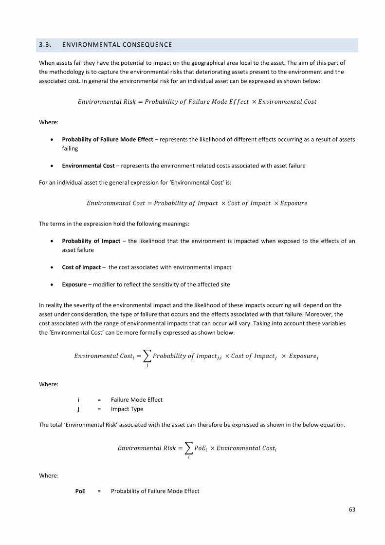
63

3.3. ENVIRONMENTAL CONSEQUENCE

When assets fail they have the potential to Impact on the geographical area local to the asset. The aim of this part of

the methodology is to capture the environmental risks that deteriorating assets present to the environment and the

associated cost. In general the environmental risk for an individual asset can be expressed as shown below:

𝐸𝑛𝑣𝑖𝑟𝑜𝑛𝑚𝑒𝑛𝑡𝑎𝑙 𝑅𝑖𝑠𝑘 = 𝑃𝑟𝑜𝑏𝑎𝑏𝑖𝑙𝑖𝑡𝑦 𝑜𝑓 𝐹𝑎𝑖𝑙𝑢𝑟𝑒 𝑀𝑜𝑑𝑒 𝐸𝑓𝑓𝑒𝑐𝑡 × 𝐸𝑛𝑣𝑖𝑟𝑜𝑛𝑚𝑒𝑛𝑡𝑎𝑙 𝐶𝑜𝑠𝑡

Where:

Probability of Failure Mode Effect – represents the likelihood of different effects occurring as a result of assets

failing

Environmental Cost – represents the environment related costs associated with asset failure

For an individual asset the general expression for ‘Environmental Cost’ is:

𝐸𝑛𝑣𝑖𝑟𝑜𝑛𝑚𝑒𝑛𝑡𝑎𝑙 𝐶𝑜𝑠𝑡 = 𝑃𝑟𝑜𝑏𝑎𝑏𝑖𝑙𝑖𝑡𝑦 𝑜𝑓 𝐼𝑚𝑝𝑎𝑐𝑡 × 𝐶𝑜𝑠𝑡 𝑜𝑓 𝐼𝑚𝑝𝑎𝑐𝑡 × 𝐸𝑥𝑝𝑜𝑠𝑢𝑟𝑒

The terms in the expression hold the following meanings:

Probability of Impact – the likelihood that the environment is impacted when exposed to the effects of an

asset failure

Cost of Impact – the cost associated with environmental impact

Exposure – modifier to reflect the sensitivity of the affected site

In reality the severity of the environmental impact and the likelihood of these impacts occurring will depend on the

asset under consideration, the type of failure that occurs and the effects associated with that failure. Moreover, the

cost associated with the range of environmental impacts that can occur will vary. Taking into account these variables

the ‘Environmental Cost’ can be more formally expressed as shown below:

𝐸𝑛𝑣𝑖𝑟𝑜𝑛𝑚𝑒𝑛𝑡𝑎𝑙 𝐶𝑜𝑠𝑡𝑖 =∑𝑃𝑟𝑜𝑏𝑎𝑏𝑖𝑙𝑖𝑡𝑦 𝑜𝑓 𝐼𝑚𝑝𝑎𝑐𝑡𝑗,𝑖 × 𝐶𝑜𝑠𝑡 𝑜𝑓 𝐼𝑚𝑝𝑎𝑐𝑡𝑗 × 𝐸𝑥𝑝𝑜𝑠𝑢𝑟𝑒𝑗

𝑗

Where:

i = Failure Mode Effect

j = Impact Type

The total ‘Environmental Risk’ associated with the asset can therefore be expressed as shown in the below equation.

𝐸𝑛𝑣𝑖𝑟𝑜𝑛𝑚𝑒𝑛𝑡𝑎𝑙 𝑅𝑖𝑠𝑘 =∑𝑃𝑜𝐸𝑖 × 𝐸𝑛𝑣𝑖𝑟𝑜𝑛𝑚𝑒𝑛𝑡𝑎𝑙 𝐶𝑜𝑠𝑡𝑖𝑖

Where:

PoE = Probability of Failure Mode Effect

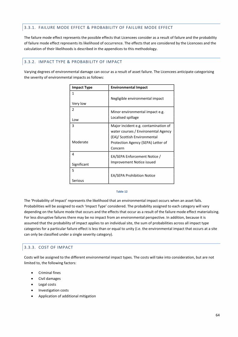
64

3.3.1. FAILURE MODE EFFECT & PROBABILITY OF FAILURE MODE EFFECT

The failure mode effect represents the possible effects that Licencees consider as a result of failure and the probability

of failure mode effect represents its likelihood of occurrence. The effects that are considered by the Licencees and the

calculation of their likelihoods is described in the appendices to this methodology.

3.3.2. IMPACT TYPE & PROBABILITY OF IMPACT

Varying degrees of environmental damage can occur as a result of asset failure. The Licencees anticipate categorising

the severity of environmental impacts as follows:

Impact Type Environmental Impact

1

Negligible environmental impact Very low

2 Minor environmental impact e.g.

Localised spillage Low

3 Major incident e.g. contamination of

water courses / Environemtal Agency

(EA)/ Scottish Environmental

Protection Agency (SEPA) Letter of

Concern

Moderate

4 EA/SEPA Enforcement Notice /

Improvement Notice issued Significant

5

EA/SEPA Prohibition Notice Serious

Table 12

The ‘Probability of Impact’ represents the likelihood that an environmental impact occurs when an asset fails.

Probabilities will be assigned to each ‘Impact Type’ considered. The probability assigned to each category will vary

depending on the failure mode that occurs and the effects that occur as a result of the failure mode effect materialising.

For less disruptive failures there may be no impact from an environmental perspective. In addition, because it is

assumed that the probability of impact applies to an individual site, the sum of probabilities across all impact type

categories for a particular failure effect is less than or equal to unity (i.e. the environmental impact that occurs at a site

can only be classified under a single severity category).

3.3.3. COST OF IMPACT

Costs will be assigned to the different environmental impact types. The costs will take into consideration, but are not

limited to, the following factors:

Criminal fines

Civil damages

Legal costs

Investigation costs

Application of additional mitigation

65

3.3.3.1. CRIMINAL FINES

Criminal fines in the context of damage to the environment will usually stem from contamination of land, air or water.

This is dealt with by the following legislation:

Illegal Discharges to air, land and water

o Environmental Protection Act 1990 (section 33)

o Environmental Permitting (England and Wales) Regulations 2010 (regulations 12 and 38(1), (2) and (3))

Breach of Duty of care

o Environmental Protection Act 1990 (section 34)

Restrictions on use of public sewers

o Water Industry Act 1991 (section 111)

Or through the equivalent legislation in Scotland which includes:

The Water Environment (Controlled Activities)(Scotland) Regulations 2011

Sewerage (Scotland ) Act 1968

In order to impose a sentence post fining the court must determine the category of the offence using culpability and

harm factors. This is set out in The Sentencing Council, Environmental Offences, 2015. In Scotland, The Sentencing

Council Scotland is currently drafting the Environmental and wildlife Offences guidelines, which are due to be published

in 2018/19.

Culpability factors are derived by the court from elements present in the case presented which are taken into account

to reach a fair assessment of culpability. For environmental offences this is split into four categories: [Sentencing

Guidelines 2015]

Deliberate

o Intentional breach or flagrant disregard, with the breach directly attributable to the organisation

o Or, deliberate failure to put in place and enforce such systems as could be reasonably expected

Reckless

o Actual foresight of, or wilful blindness to the risk of offending but risk was taken no the less by

someone whose position of authority in the organisation makes it directly attributable

o Or, deliberate failure to put in place and enforce such systems as could be reasonably expected

Negligent

o Failure to take reasonable care and put in place and enforce proper systems to avoid commission of

the offence

Low Culpability

o Offence committed with little or no fault on the part of the organisation

o Presence and due enforcement of all reasonably required preventive measures

o Proper preventive measures were unforeseeably overcome by exceptional events

66

Harm is assessed by the court into one of four categories: [Sentencing Guidelines 2015]

Category 1

o Polluting material of a dangerous nature

o Major adverse effect or damage to air or water quality, amenity value, or property

o Polluting material was noxious, widespread or pervasive with long-lasting effects on human health or

quality of life, animal health or flora

o Major costs incurred through clean-up, site restoration or animal rehabilitation

o Major interference with, prevention or undermining of other lawful activities or regulatory regime due

to offence

Category 2

o Significant adverse effect or damage to air or water quality, amenity value, or property

o Significant adverse effect on human health or quality of life, animal health or flora

o Significant costs incurred through clean-up, site restoration or animal rehabilitation

o Significant interference with or undermining of other lawful activities or regulatory regime due to

offence

o Risk of category 1 harm

Category 3

o Minor, localised adverse effect or damage to air or water quality, amenity value, or property

o Minor adverse effect on human health or quality of life, animal health or flora

o Low costs incurred through clean-up, site restoration or animal rehabilitation

o Limited interference with or undermining of other lawful activities or regulatory regime due to

offence


Category 4


It is assumed that as a prudent operator and/or owner any incident that occurred would fall into the low culpability

category. This is the justification for the inclusion of additional mitigation costs so as that post incident the level of

culpability does not increase.

Similarly to the above statement it is assumed that in assessment of harm a prudent operator is unlikely to exceed

category 2 harm in the extreme. The primary route to category 2 harm is anticipated to be significant clean-up cost

incurred for certain types of incident.

When a fine is applied by the court this is determined on the basis of the company revenue with the aim of fines being

proportionate. As this is the case company specific appendices will be provided per company due to differences in

revenue. These appendices will be revised upon re-issue of the Sentencing Council Guidelines, material changes to

legislation and precedent or significant changes to company revenue.

Tables for fines relating to environmental offences will be given in the Specific Appendices.

67

3.3.3.2. CIVIL DAMAGES

In the UK environmental legislation is based on the polluter pays principle. For simplicity of this model provision will be

made for remediation cost as part of the cost of recovery appendices. The main routes for incurring cost would be

through damages to property and amenity and nuisance. This is covered by:

Environmental Damage (Prevention and Remediation) Regulations 2009

Or in Scotland, Environmental Liability (Scotland) Regulations 2009

The regulations reinforce the polluter pays principle making organisations financially liable for damage to land, water

and biodiversity. It is anticipated that a prudent operator would take all reasonable steps to remedy damage caused.

3.3.3.3. INVESTIGATION AND LEGAL COSTS

All incidents that occur must be investigated ranging from a near miss to the most serious incidents. Due to the nature

and complexity of investigations, a range will be provided in the Specific Appendices.

Legal costs are to be included to give a more accurate representation of risk management costs. As with cost of

investigations these cost will vary on the case. A table will be provided in the Specific Appendices, making an

approximation based on case studies for legal cost relating to the highest impact implied by criticality.

3.3.3.4. APPLICATION OF ADDITIONAL MITIGATION

When incidents are investigated and reviewed it is likely that number of additional mitigations will be identified to

ensure that the outcome remains an isolated incident. Additional mitigations can range from improved systems or

training to acceleration of asset replacement programmes. The application of additional measures is part of managing

risk and will always be applied by a prudent operator and/or owner. This is compliant with maintain safety performance

and managing network risk.

Approximated costs of additional mitigations are included in the company specific appendices. The costs are related to

asset population sizes and environmental exposure.

3.3.4. EXPOSURE

Due to the distributed nature of networks it is important that exposure is taken into account. Environmental

consequences are specific to individual assets and also their physical location. Some assets pose a greater risk to the

environment then others. In order to account for this an ‘Exposure’ modifier is incorporated into the ‘Environmental

Cost’ calculation. The TOs have yet to finalise the details on how to derive the ‘Exposure’ modifier. Table 13 provides an

indication of the factors that the Licencees anticipate will be incorporated into this calculation.

Factors for

Consideration Scope

Supporting

Information/Data/Evidence

Proximity to

Environmentally

Sensitive Sites

Considers the proximity of assets to

environmentally sensitive sites.

ESQCR Information

Site Information

Mitigation

Considers existing mitigation that

has been put in place to reduce the

likelihood/consequence of different

environmental events occurring as a

result of different failure effects.

Site information

Table 13

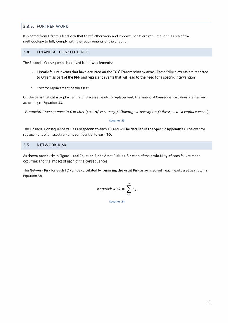
68

3.3.5. FURTHER WORK

It is noted from Ofgem’s feedback that that further work and improvements are required in this area of the

methodology to fully comply with the requirements of the direction.

3.4. FINANCIAL CONSEQUENCE

The Financial Consequence is derived from two elements:

1. Historic failure events that have occurred on the TOs’ Transmission systems. These failure events are reported

to Ofgem as part of the RRP and represent events that will lead to the need for a specific intervention

2. Cost for replacement of the asset

On the basis that catastrophic failure of the asset leads to replacement, the Financial Consequence values are derived

according to Equation 33.

𝐹𝑖𝑛𝑎𝑛𝑐𝑖𝑎𝑙 𝐶𝑜𝑛𝑠𝑒𝑞𝑢𝑒𝑛𝑐𝑒 𝑖𝑛 £ = 𝑀𝑎𝑥 (𝑐𝑜𝑠𝑡 𝑜𝑓 𝑟𝑒𝑐𝑜𝑣𝑒𝑟𝑦 𝑓𝑜𝑙𝑙𝑜𝑤𝑖𝑛𝑔 𝑐𝑎𝑡𝑎𝑠𝑡𝑟𝑜𝑝ℎ𝑖𝑐 𝑓𝑎𝑖𝑙𝑢𝑟𝑒, 𝑐𝑜𝑠𝑡 𝑡𝑜 𝑟𝑒𝑝𝑙𝑎𝑐𝑒 𝑎𝑠𝑠𝑒𝑡)

Equation 33

The Financial Consequence values are specific to each TO and will be detailed in the Specific Appendices. The cost for

replacement of an asset remains confidential to each TO.

3.5. NETWORK RISK

As shown previously in Figure 1 and Equation 3, the Asset Risk is a function of the probability of each failure mode

occurring and the impact of each of the consequences.

The Network Risk for each TO can be calculated by summing the Asset Risk associated with each lead asset as shown in

Equation 34.

𝑁𝑒𝑡𝑤𝑜𝑟𝑘 𝑅𝑖𝑠𝑘 = ∑𝐴𝑘

𝑛

𝑘=1

Equation 34

69

4. NETWORK REPLACEMENT OUTPUTS

4.1. INTERVENTIONS

Certain types of intervention will address particular failure modes. These may be routine interventions, such as

maintenance, or specific, such as planned replacements.

The available interventions for managing the performance of assets range from routine maintenance to full

replacement.

These activities are undertaken to ensure the longevity and performance of the TOs’ networks. Without effective

management of these activities, and understanding the related interactions between them, the TOs would, in time,

experience deterioration of network outputs which would have a significant detrimental impact on the capability of the

network.

Our intervention plans are optimised to deliver an efficient level of Network Risk in line with customer, consumer and

stakeholder expectation. In determining this efficient level, the TOs evaluate the cost of interventions against the

benefits these interventions deliver.

In determining an intervention plan in any period, the TOs need to assess the Asset Risks and decide exactly which

interventions to undertake. This requires the TOs to make a binary decision (e.g. to replace, or not to replace) where

every asset has an Asset Risk contribution to the Network Risk. This process involves assessing all available interventions

(both OPEX and CAPEX) to decide the combination which most efficiently manages Network Risk.

The cost of these interventions is not equal to the reduction in Network Risk achieved by undertaking that intervention

plan.

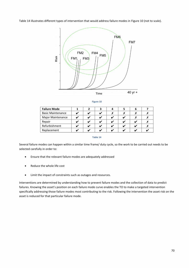
70

Table 14 illustrates different types of intervention that would address failure modes in Figure 10 (not to scale).

Figure 10

Failure Mode 1 2 3 4 5 6 7

Basic Maintenance ✔ ✔ ✔ ✗ ✗ ✗ ✗

Major Maintenance ✔ ✔ ✔ ✔ ✔ ✗ ✗

Repair ✔ ✔ ✔ ✔ ✔ ✔ ✗

Refurbishment ✔ ✔ ✔ ✔ ✔ ✔ ✗

Replacement ✔ ✔ ✔ ✔ ✔ ✔ ✔

Table 14

Several failure modes can happen within a similar time frame/ duty cycle, so the work to be carried out needs to be

selected carefully in order to:

Ensure that the relevant failure modes are adequately addressed

Reduce the whole life cost

Limit the impact of constraints such as outages and resources.

Interventions are determined by understanding how to prevent failure modes and the collection of data to predict

failures. Knowing the asset’s position on each failure mode curve enables the TO to make a targeted intervention

specifically addressing those failure modes most contributing to the risk. Following the intervention the asset risk on the

asset is reduced for that particular failure mode.

71

4.1.1. MAINTENANCE

The purpose of asset maintenance is to ensure that relevant statutory and legal requirements are met, such as those

relating to safety and environmental performance, as well as allowing the TOs to gather condition information so that

performance risks are better understood and mitigated.

Maintenance is a fundamental tool in the TOs’ management of network reliability, safety and environmental

performance (and hence customer satisfaction). Reducing maintenance to zero, or reducing levels without undertaking

impact assessments, would lead to a decline in the condition of assets (this effect is seen more rapidly than for under-

investment in replacement), leading to increased unplanned events and in some cases bringing forward the need for

asset replacement or increasing refurbishment activities.

Maintenance policy evolves as processes and practice are periodically reviewed. The TOs reassess maintenance policy

and interval decisions on an ongoing basis using the latest information available in order to ensure our assets can

achieve their anticipated asset lives and reduce the potential for unplanned disruption. Maintenance activity can

uncover developing trends for defects, ensure rectification of unforeseen functional failure modes and can enable

innovation.

When developing maintenance content and undertaking frequency reviews, the TOs have a systematic, structured

method for cost/benefit evaluation. This includes understanding the asset’s reliability for known failure modes, taking

account of how the operating costs would be expected to increase during the time between maintenance tasks,

identifying potential changes in performance and consideration of the impact that a change to the maintenance task

frequency might have on the life of the asset. As part of the planning process, maintenance is bundled into efficient

packages to optimise access to the network and the assets.

Through maintenance activities the TOs can manage the natural deterioration of asset condition so that the assets

remain operable throughout their anticipated technical life, reducing unplanned outages on the network as well as

monitoring the condition of assets to improve understand of their performance. This then feeds into future asset

intervention plans.

Maintenance activities are pro-active interventions which take place at regular intervals according to policy.

Undertaking maintenance activities ensures that the assets function correctly and can identify issues with the assets

which can be addressed prior to a failure mode occurring.

A basic maintenance will involve basic checks for function of particular components as well as activities such as visual

inspections, checks for fluid/gas levels where appropriate.

An intermediate maintenance takes place at longer intervals than a basic and will include all activities undertaken for a

basic maintenance but will include additional checks on specific components of the equipment.

A major maintenance will include all the activities undertaken for a basic and intermediate maintenance but will also

include comprehensive and possibly intrusive work as well as more exhaustive checks. These take place less regularly

than basic and intermediate levels and generally require a significantly longer outage to carry out the work.

The intervals for the maintenance activities are determined through maintenance policy for each asset type, according

to the specific requirements for that asset and manufacturer recommendations are also taken into account.

72

4.1.2. REPAIR

Repair is a reactive activity responding to a failure mode when it has occurred or, in some cases, to prevent a particular

failure mode if it can be detected before failure occurs. For some failure modes which cannot be detected on a routine

basis, such as by maintenance or inspection, repair is the only available intervention once the failure mode has

occurred. That is not to say that detection of the failure mode is not available and assets are monitored for known

failure modes. For example, cable oil pressure is monitored and an alarm triggered if the pressure falls below a certain

level. The failure mode is detected as the oil leak initiates but there are no routine interventions available to detect the

occurrence of a leak before it occurs.

The only available option is to repair the cable when the oil leak is detected. Some failure modes, which lead to another

failure mode, can be detected prior to failure, for example, sheath testing of cables will reveal defects in the oversheath

which, if left unrepaired, will eventually lead to the corrosion of the sheath and subsequently an oil leak. A repair

intervention can then be planned to mitigate this risk.

4.1.3. REFURBISHMENT

The decision to refurbish instead of replace an asset follows careful consideration of a number of criteria. For

refurbishment to be technically feasible and cost-effective, the asset population size must be sufficiently large because

the costs associated with developing the technical content of a refurbishment procedure, and the set-up costs to

undertake the work, mean that it is difficult to make refurbishment of small populations cost-effective.

The ongoing lifetime cost of supporting a refurbished asset family must also be considered. It may be more cost-

effective to replace highly complex units that require frequent intervention.

Continuing spares support must be considered. Whilst some spares can be re-engineered without significant risk, this is

not appropriate for performance critical components. If such components are unavailable (or not available cost-

effectively), refurbishment is unlikely to be a realistic option.

Additionally, the condition and deterioration mechanisms of the asset class must be well understood. If these criteria

are met, and it is considered that refurbishment is a viable option, it would be expected that refurbishment activities

would change the asset’s condition and/or extend asset life.

4.1.4. REPLACEMENT

Individual assets or families which are deemed to be a priority given their risk trigger the need for replacement and

capital investment. To facilitate the development of an optimised replacement plan, priority ranked lists for

replacement are created for each asset type.

73

4.2. ASSETS REQUIRING SEPARATE TREATMENT

4.2.1. HIGH IMPACT, LOW PROBABILITY EVENTS

A significant amount of work has been undertaken by the TOs with respect to High Impact, Low Probability events. This

work will be directly fed into the cross sector (Electricity and Gas, Transmission and Distribution) working that has been

initiated by Ofgem.

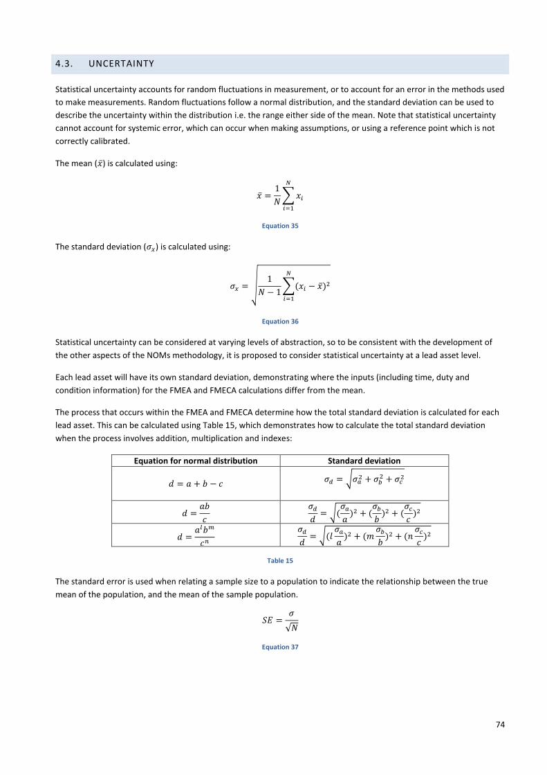
74

4.3. UNCERTAINTY

Statistical uncertainty accounts for random fluctuations in measurement, or to account for an error in the methods used

to make measurements. Random fluctuations follow a normal distribution, and the standard deviation can be used to

describe the uncertainty within the distribution i.e. the range either side of the mean. Note that statistical uncertainty

cannot account for systemic error, which can occur when making assumptions, or using a reference point which is not

correctly calibrated.

The mean (�̅�) is calculated using:

�̅� =1

𝑁∑𝑥𝑖

𝑁

𝑖=1

Equation 35

The standard deviation (𝜎𝑥) is calculated using:

𝜎𝑥 = √1

𝑁 − 1∑(𝑥𝑖 − �̅�)

2

𝑁

𝑖=1

Equation 36

Statistical uncertainty can be considered at varying levels of abstraction, so to be consistent with the development of

the other aspects of the NOMs methodology, it is proposed to consider statistical uncertainty at a lead asset level.

Each lead asset will have its own standard deviation, demonstrating where the inputs (including time, duty and

condition information) for the FMEA and FMECA calculations differ from the mean.

The process that occurs within the FMEA and FMECA determine how the total standard deviation is calculated for each

lead asset. This can be calculated using Table 15, which demonstrates how to calculate the total standard deviation

when the process involves addition, multiplication and indexes:

Equation for normal distribution Standard deviation

𝑑 = 𝑎 + 𝑏 − 𝑐 𝜎𝑑 = √𝜎𝑎

2 + 𝜎𝑏2 + 𝜎𝑐

2

𝑑 =𝑎𝑏

𝑐

𝜎𝑑𝑑= √(

𝜎𝑎𝑎)2 + (

𝜎𝑏𝑏)2 + (

𝜎𝑐𝑐)2

𝑑 =𝑎𝑙𝑏𝑚

𝑐𝑛

𝜎𝑑𝑑= √(𝑙

𝜎𝑎𝑎)2 + (𝑚

𝜎𝑏𝑏)2 + (𝑛

𝜎𝑐𝑐)2

Table 15

The standard error is used when relating a sample size to a population to indicate the relationship between the true

mean of the population, and the mean of the sample population.

𝑆𝐸 =𝜎

√𝑁

Equation 37

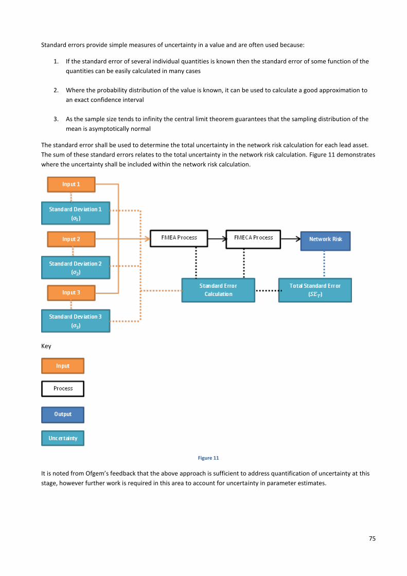
75

Standard errors provide simple measures of uncertainty in a value and are often used because:

1. If the standard error of several individual quantities is known then the standard error of some function of the

quantities can be easily calculated in many cases

2. Where the probability distribution of the value is known, it can be used to calculate a good approximation to

an exact confidence interval

3. As the sample size tends to infinity the central limit theorem guarantees that the sampling distribution of the

mean is asymptotically normal

The standard error shall be used to determine the total uncertainty in the network risk calculation for each lead asset.

The sum of these standard errors relates to the total uncertainty in the network risk calculation. Figure 11 demonstrates

where the uncertainty shall be included within the network risk calculation.

Key

Figure 11

It is noted from Ofgem’s feedback that the above approach is sufficient to address quantification of uncertainty at this

stage, however further work is required in this area to account for uncertainty in parameter estimates.

76

5. ASSUMPTIONS

Term Symbol Determination of Term

P-F Failure Mode N/A TO experience using all available information: Based on manufacturer information, understanding of asset design, technical specifications, innovation project results, failure investigation reports, failure, faults and defects data, forensics results, evidence from interventions, information from other network operators (international)

Utilisation Failure Mode N/A TO experience using all available information: Based on manufacturer information, understanding of asset design, technical specifications, innovation project results, failure investigation reports, failure, faults and defects data, forensics results, evidence from interventions, information from other network operators (international)

Random Failure Mode N/A TO experience using all available information: Based on manufacturer information, understanding of asset design, technical specifications, innovation project results, failure investigation reports, failure, faults and defects data, forensics results, evidence from interventions, information from other network operators (international)

Appropriate interventions N/A TO experience using all available information: Based on manufacturer information, understanding of asset design, innovation project results, failure investigation reports, failure, faults and defects data, forensics results, evidence from interventions, reviews of intervention policy, information from other network operators (international)

P(Failure) Time since last intervention N/A Data driven: Data driven from installation date and completed interventions

P(Failure) Number of operations since last intervention

N/A Data driven: Data driven from operations counters and from SCADA information

P(Failure) Condition N/A Data driven: Condition data, performance data

Failure rate per asset per year N/A TO experience using all available information: Based on manufacturer information, understanding of asset design, innovation project results, failure investigation reports, failure, faults and defects data, forensics results, evidence from interventions, reviews of intervention policy, information from other network operators (international)

77

Modifier for location/environment/family N/A TO experience using all available information: Location data, environment data, asset family data. Experience of how location, environment, asset family impacts failure rate based on manufacturer information, understanding of asset design, innovation project results, failure investigation reports, failure, faults and defects data, forensics results, evidence from interventions, reviews of intervention policy, information from other network operators (international).

Probability of failure N/A Calculated term

Others parameters and terms have been explained within sections (i.e. Section 4.1) or within the Appendices to the

Methodology.

6. RISK TRADING MODEL

The Risk Trading Model will calculate the monetised risk for each asset and aggregate to give the total Network Risk. It

will reflect the processes and calculations described within this methodology and associated appendices.

7. CALIBRATION, TESTING AND VALIDATION

A detailed plan for calibration, validation and testing accompanies this issue of the methodology. The methodology has

been designed to enable the parameters to be easily adjusted to reflect the results of the testing, validation and

calibration exercises. The calibration, validation and testing will include scenarios and tests where defined criteria are

set out prior to the test and the results are compared against these criteria.

CALIBRATION

Ensure consistency in the application of the methodology. All three TOs will work together to ensure that the

application of this methodology is consistent.

CALIBRATION OF CONDITION

All three TOs will compare their asset condition information. It is expected that for assets in the same condition with the

same history, operating regime, operating environment and duty, each asset would expect to have the same probability

of failure for all TOs.

CALIBRATION OF CONSEQUENCE

Consequence of failure will be compared across the TOs. Where it is possible to compare consequences, these would be

expected to have the same scores for the same criteria. It is expected that safety and environmental consequence

scoring would demonstrate a greater degree of consistency between the TOs.

However, due to the differing scales of the TOs respective networks, there may be some instances where specific

criticality score may need to be used, most notably with system consequence. The TOs can compare the ratio of

consequence scores that fall into the very high, high, medium and low categories to ensure a consistency of approach.

78

TESTING

In order to test the monetised network risk, the spreadsheet models for each asset group will be populated with data.

Asset risk will be calculated for current condition and forecast condition for each asset group.

An independent expert will be appointed to check the spreadsheet and provide assurance that its internal calculations

are correct, verifying that the models perform according to this methodology.

VALIDATION

Validation that the PoF and consequence values calculated by the methodology are consistent with actual outcomes

The probabilities of failure will be validated periodically by ensuring the summated values are consistent with actual

asset performance. The consequence monetary values will be validated periodically by adding new events as they occur

and comparing them against the value being used.

Confirmation that the number of assets planned for intervention is consistent with the need for intervention

Validation of this methodology will involve confirmation that the numbers of assets that are expected to be replaced or

refurbished over the RIIO-T1 period is consistent with the TOs’ investment plans. This involves monitoring the network

risk with intervention and network risk without intervention. The difference between these network risk positions will

confirm whether the TOs’ investment plans reflect the number of assets that are planned for replacement or

refurbishment is consistent with the need for intervention.

79

APPENDICES TO METHODOLOGY

APPENDIX I - IMPLEMENTATION OF THE INCENTIVE MECHANISM FOR RIIO-T1

For the RIIO-T1 submission, the Network Replacement Outputs targets encoded into Special Licence Condition 2M were

set based on the forecast of expected Replacement Priorities at 31 March 2021. To generate this forecast of expected

Replacement Priorities the TOs used forecast asset deterioration and the forecast investment plans for the RIIO-T1

period.

As part of the RIIO-T1 price control review, Ofgem assessed the TOs forecast asset deterioration and forecast

investment plans and subsequently adopted the forecast asset replacement priorities at 31 March 2021 as the basis of

the Network Replacement Outputs.

To align with the intent of maintaining reliability at historic levels, the forecast investment plans were developed to

keep the network risk at a level similar at the end of RIIO-T1, as it was at the beginning of RIIO-T1 in line with

stakeholder expectations.

The following quotations relate to reliability NGET stakeholder engagement sessions held for Energy Not Supplied:

“In terms of the current level of reliability from National Grid, attendees were in general very happy, and expressed a

desire for it to be maintained at its current level for the next 20-30 years. However, they did acknowledge that this would

come at a cost”.

Stage one workshop Brunswick report, 10th December 2010

“Reliability is not something on which most participants are willing to compromise – it’s widely expected to remain at

current levels (or higher).”

Stage one workshop Brunswick report, 19th January 2011

There are two principle sources of uncertainty around the forecast of network risk:

1. Forecasting of asset deterioration

2. Unexpected type faults

Asset deterioration is inherently uncertain and probabilistic modelling techniques are used to forecast condition. The

forecast Replacement Priorities at 31 March 2021 were based on the median value and thus expected forecast of

network risk.

Unexpected type faults cannot be forecast but can have a significant impact on network risk, causing significant cost

and disruption of the investment plan. It would not be sensible to model this risk probabilistically so these were not

included in the forecast replacement priorities.

USING THE NETWORK OUTPUT MEASURES

The TOs’ NOMs are used internally to enhance current asset management processes and understanding of business

drivers. This is especially in relation to the development, maintenance and operation of our networks and in assessing

future network expenditure.

In addition to the joint methodology statement, the TOs have developed specific appendices which describe how they

use the NOMs within our respective businesses. These specific appendices are confidential.

80

Under RIIO-T1, the TOs have each developed integrated business plans which are supported by a suite of mechanisms

designed to help manage the uncertainty that the electricity industry faces over the next decade. Non-load related

activities are the capital and direct operating elements of the plan which are focused on maintaining performance of

our assets through replacement, refurbishment and maintenance.

Through these activities, the TOs’ intention is to improve our safety and environmental performance whilst maintaining

reliability (in terms of Energy Not Supplied) at current levels. These activities are targeted at delivering stakeholders’

requirements, from connecting new supplies to providing a safe, reliable service.

The TOs’ business plans are designed to manage the ongoing safety, reliability and environmental performance of our

networks. The potential customer impact associated with the deteriorating performance of assets towards the end of

their useful life continues to drive a programme of interventions on our transmission network assets.

The TOs manage interventions on our equipment to ensure that:

a. The number, severity and criticality of equipment failures are acceptable to the TOs and our stakeholders

b. Long term replacement plans can be achieved without having an unacceptable impact on reliability,

availability, quality of supply, health, safety and environmental performance, and transmission constraints

c. Long term capital forecasts are within acceptable levels for efficient deliverability, procurement and

financing requirements

The available interventions for managing the performance of assets range from routine maintenance to full

replacement. At the highest level, there are three options for intervention for each lead plant type which have

definitions agreed with Ofgem:

a. Maintenance

b. Refurbishment

c. Replacement

DECISION MAKING

These three activities are undertaken to ensure the longevity and performance of the TOs’ networks. Without effective

management of these activities, and understanding the related interactions between them, the TOs would, in time,

experience deterioration of network outputs which would have a significant detrimental impact on the capability of the

network.

Figure 1 shows how the process by which elements of NOMs feed into an investment plan. Health criteria (e.g.

condition, performance) categorised into AHIs represent the Network Asset Condition. These AHIs are combined with

information about Criticality to determine Replacement Priorities. These Replacement Priorities are combined with

other factors (e.g. outages, resources) to determine scheme priority which is used to determine the investment plan.

81

Figure 12

The Risk represents the level of Network Risk held on the system and has been developed in a way that ensures a

consistent understanding of risk across all asset types. They take into account changes to asset populations, including

load and non-load related replacement volumes.

The Risk determines the Network Replacement Outputs, providing Ofgem with the ability to monitor and assess the

TOs’ asset management performance. The non-load related targets for the Network Replacement Outputs are coded

into the respective licences for each TO in Special Licence Condition 2M. The process for setting the targets is discussed

in section 2.3 and illustrated in Figure 3.

Network Performance is currently monitored through the Average Circuit Unreliability (ACU) metric, which represents

network unavailability as a result of asset unreliability. This metric records the impact of Functional Failures and is used

to understand the impact of unreliability on the TOs’ networks.

Work has been undertaken to further understand the relationship between asset condition and network performance.

The ACU is presented in a format that disaggregates the metric by equipment group and then by asset condition. Figure

2 shows the conceptual relationship between Energy Not Supplied events and other network performance metrics. The

TOs are continuously developing their understanding of the relationship between Asset Health and Network

Performance.

Asset Management Information

Criticality Information

Deliverability (resources,

outages etc)

Probability of Failure

Consequence of Failure

Scheme Prioritisation

Other Intervention Drivers (load,

safety etc)

Forecast Probability of

Failure

Risk

Network Replacement

Outputs

Compare with Targets

Meets RIIO Target?

No Work Plan

Yes

Continual Review/

Innovation

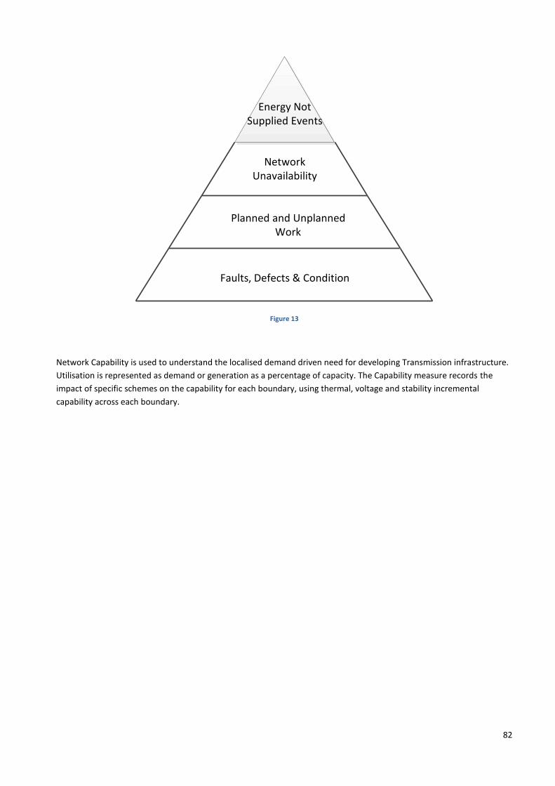
82

Figure 13

Network Capability is used to understand the localised demand driven need for developing Transmission infrastructure.

Utilisation is represented as demand or generation as a percentage of capacity. The Capability measure records the

impact of specific schemes on the capability for each boundary, using thermal, voltage and stability incremental

capability across each boundary.

Energy Not Supplied Events

Network Unavailability

Planned and Unplanned Work

Faults, Defects & Condition

83

REPORTING TO THE AUTHORITY


The NOMs will be reported to Ofgem as part of the annual Transmission Regulatory Reporting Packs (RRP) as required in

Standard Licence Condition B15: Regulatory Instructions and Guidance (RIGs).

Licence Condition 2L.6 requires that the TOs provide information (whether historic, current or forward-looking) about

the NOMs supported by such relevant other data and examples of network modelling, as may be specified for the

purposes of this condition in any RIGs that have been issued by the Authority in accordance with the provisions of

Standard Licence Condition B15.

Network Output Measure Reported in RRP Table

Network Asset Condition 6.15.1_NOMs_detail

Network Risk 6.15.2_NOMs_RP

Network Performance 5.10_ACU

Network Capability 5.3_Boundary_Tran_Requirements 5.4_Bound_Capab_Dev 5.5_Demand_&_Supply_Sub

Network Replacement Outputs 6.15.2_NOMs_RP

In addition to the submitted tables, the TOs provide a narrative which explains changes to the outputs from the

previous year.

REPORTING TIMESCALES

The reporting year for the provision of information is from 1 April to 31 March the following calendar year. The

information required under the RIGs will be provided not later than 31 July following the end of the relevant reporting

year.

For the RIIO-T1 period, the first reporting period was 1 April 2013 to 31 March 2014.

DATA ASSURANCE

Licence Condition B23 requires each TO to undertake processes and activities for the purpose of reducing the risk, and

subsequent impact and consequences, of any inaccurate or incomplete reporting, or any misreporting, of information to

the Authority.

To ensure compliance with this licence condition, each TO carries out risk assessments to understand the implications of

reporting inaccurate, inconsistent or incomplete data. Each NOM table reported in the RRP has undergone such a risk

assessment. Where improvements can be made to data systems or processes, actions are planned that are

proportionate to the risk of a submission in order to reduce the impact of inaccuracies in the submissions.

In providing data the TOs have developed work instructions for each table to be submitted to ensure a consistent

approach.

Data concerning the asset inventory, condition scoring and criticality information is specific to each TO. Details about

the type and quantity of data are described in each Specific Appendix.

Specifically, these describe the data that informs health indices and how it is used for specific assets. They indicate the

volume of available data and whether any data has to be inferred. They explain whether there is any blanket

replacement of certain assets and associated reasons. These also describe how any limitations in the data affect the

confidence in scoring for health and criticality and how any uncertainties can be quantified.

84

NETWORK PERFORMANCE


Paragraph 2L.4(c) of Special Licence Condition requires the TOs to enable the Evaluation of:

“Those aspects of the technical performance of the TO’s Transmission system which have a direct impact on the

reliability and cost of services provided the TO as part of its Transmission business (Network Performance)”

The key elements from this Special Licence Condition are:

a. Performance of the TO’s Transmission system

b. Direct impact on the reliability and cost of the services

METHODOLOGY

Network Performance is a key output for the customers of the TOs. To provide a full picture on Network Performance, it

is necessary to consider a number of complementary performance measures. This is because some measures consider

events only and some consider a combination of event and duration.

Reduced reliability of the Transmission network increases the risk of loss of supply for directly connected customers and

increased costs to market participants which impact the consumer. An increased number of loss of supply events

creates a cost of inconvenience to the general consumer and in extreme cases will result in a significant impact upon

the economy.

Average Circuit Unreliability (ACU) is derived from the unavailability of the network due to outages occurring as a result

of unreliability events which cannot be deferred until the next planned intervention and is defined in Equation 38

below.

period timereported ofDuration * Circuits ofNumber

circuits) across e(cumulativRepair ofDuration Total

Equation 38: Average Circuit Unavailability

Duration in the context of ACU is a continuous number and is not rounded or truncated at any stage of the calculation,

thus no errors are introduced into the calculation.

The monthly duration is calculated using a differing number of days in a month and so any calculation to derive a yearly

number will require a suitable weighting of monthly values to account for this.

The outages which are classified as being included within the definition of ACU are:

a. Enforced unreliability outages taken at less than 24 hours’ notice (otherwise known as unplanned

unavailability)

b. Planned unreliability outages taken after 24 hours’ notice

All unreliability related outages are included within the definition of ACU. The definition above assumes that no outages

are planned with less than 24 hours’ notice as any such outage would fall into part a. in the definition above.

85

The TOs have investigated whether the Fault and Failure data provides a statistically significant dataset to derive

correlations with asset condition. The actual number of Faults and Failures is very small across all the TOs. This is a

result of:

a. Actual population sizes of the assets. The population is not large enough to experience a great number of

reliability related Faults and Failures

b. Asset management approach within the business. The TOs maintain assets to manage the number of faults

experienced an aim to replace before failure using AHI and Criticality to prioritise asset replacement

candidates. This means many Faults and Failures that might occur are avoided.

The number of Faults and Failures has proven insufficient to enable accurate correlations with asset condition. Details

of the investigations undertaken by each TO are included in the existing respective TOs’ Specific Appendices.

By looking at Functional Failures, there is a greater set of data which can be used for correlation with asset condition.

Functional Failures include those unreliability related outages which are used to determine ACU.

Each TO has varying historical datasets with which to produce correlation of asset unreliability with asset condition. In

addition, given the introduction of AHIs on a consistent basis across the TOs, there is limited historical condition

information to provide correlation with Functional Failures. These historical datasets will grow with time and thus the

accuracy of the correlations will improve.

The investigations undertaken by each TO include the analysis undertaken to identify correlations between asset

unreliability and asset condition are detailed in the TOs’ Specific Appendices.

ENSURING CONSISTENCY

The ACU is calculated consistently using the same definitions in line with the RIGs for all TOs.

The calculation to determine Energy Not Supplied for incentivised loss of supply events according to transmission

licence condition 3C is based upon a joint methodology statement. This was developed jointly between all transmission

TOs and is therefore applied consistently.

REPORTING

The TOs report a comprehensive set of Network Performance measures in the form of Energy Not Supplied (Table 6.3),

Average Circuit Unavailability (Table 5.10) as well as Faults and Failures information (Table 5.2) with associated

commentary through the Transmission RRP.

For ACU, the total number of circuits used in this calculation varies by TO and will vary from year to year as the

networks are modified. For this reason, the number of circuits used as part of the ACU calculation is reported as at 31

March each year.

CONTINUOUS IMPROVEMENT

The TOs will continue to assess the performance of their assets and, through monitoring these metrics, will use them to

develop strategies to manage asset unreliability.

EXTERNAL PUBLICATION

There are no issues with the external publication of the NOMs methodology for Network Performance. The summary

tables as reported in the Transmission RRP should not be published externally.

86

NETWORK CAPABILITY


Paragraph 2L.4(d) of the Special Licence Condition requires the TOs to enable the evaluation of:

“The Network Capability measure, which relates to the level of the capability and utilisation of the TO’s Transmission

system at entry and exit points and to other network capability and utilisation factors”

The key elements from this Special Licence Condition are:

a. Information about Transmission system capability

b. Information about Transmission system utilisation

METHODOLOGY

The TOs report on Transmission system capability as part of the Transmission RRP which monitors the existing

Transmission capacity being provided by the TOs on the NETS.

Likewise, the Transmission RRP requires the individual TOs to collect information relating to more localised demand

driven needs for developing transmission infrastructure. This is presented in Table 5.5 with utilisation being represented

as demand as a percentage of capacity. This shows the relationship between localised demand and capacity and hence

provides a proxy measure for utilisation.

Adopting these measures ensures consistency in reporting and interpretation of requirements across all TOs.

PROVISION OF INFORMATION ON VOLTAGE AND STABILITY (THERMAL)

Information is reported in the ETYS at a boundary level. This boundary capability is calculated based on the most

onerous limitation whether this is thermal or voltage.

Where stability constrains boundary capability this data will be provided where it is available.

Transmission RRP Table 5.4 reports present year boundary capability and incremental capability for the reinforcement

completed in the present year.

ENSURING CONSISTENCY

Capability and utilisation is reported by the TOs in a consistent manner according to the RIGS. As described earlier,

demand is represented as a percentage of capacity, hence ensuring a consistency of reporting despite the differing

scales of the respective TOs’ networks.

REPORTING

Tables 5.3 and 5.4 of the Transmission RRP reflect the capability requirement and boundary capability for all RIIO

boundaries. Table 5.5 reflects the utilisation requirement.

Table 5.3 collects information on Transmission capacity against required transfer levels at key parts of the Transmission

system.

Actual capability information is provided in Table 5.4 and reflects the impact of specific schemes on the capability for

each boundary. For each scheme the thermal, voltage and stability incremental capability across each boundary is

87

given. In addition, the Table shows the capabilities at the start of the reporting period and the final overall capability

(based on all schemes). The RIGs provide the rules for creating Table 5.4.

The rules for creating Table 5.5 are also taken form the RIGs. Information will be used from the most recent business

planning studies. Further rules are as follows:

a. Peak Demand: the maximum demand of the demand group at the substation

b. Maintenance Period Demand: as defined in the NETS SQSS

c. n-1 Capacity: the first circuit outage condition as defined in the NETS SQSS

d. n-2 Capacity (300 MW demand groups only): the second circuit outage condition as set out in the NETS

SQSS. This is only applicable for substations where the peak group demand is greater than 300 MW.

CONTINUOUS IMPROVEMENT

The TOs will continue to review the submitted information for Network Capability.

EXTERNAL PUBLICATION

There are no issues with the external publication of the proposed NOMs methodology for Network Capability. The

summary tables which form part of the Transmission RRP should not be published externally. The Specific Appendices

should not be published.

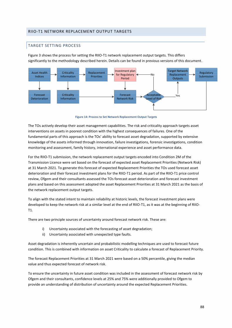
88

RIIO-T1 NETWORK REPLACEMENT OUTPUT TARGETS

TARGET SETTING PROCESS

Figure 3 shows the process for setting the RIIO-T1 network replacement output targets. This differs

significantly to the methodology described herein. Details can be found in previous versions of this document.

Figure 14: Process to Set Network Replacement Output Targets

The TOs actively develop their asset management capabilities. The risk and criticality approach targets asset

interventions on assets in poorest condition with the highest consequences of failures. One of the

fundamental parts of this approach is the TOs’ ability to forecast asset degradation, supported by extensive

knowledge of the assets informed through innovation, failure investigations, forensic investigations, condition

monitoring and assessment, family history, international experience and asset performance data.

For the RIIO-T1 submission, the network replacement output targets encoded into Condition 2M of the

Transmission Licence were set based on the forecast of expected asset Replacement Priorities (Network Risk)

at 31 March 2021. To generate this forecast of expected Replacement Priorities the TOs used forecast asset

deterioration and their forecast investment plans for the RIIO-T1 period. As part of the RIIO-T1 price control

review, Ofgem and their consultants assessed the TOs forecast asset deterioration and forecast investment

plans and based on this assessment adopted the asset Replacement Priorities at 31 March 2021 as the basis of

the network replacement output targets.

To align with the stated intent to maintain reliability at historic levels, the forecast investment plans were

developed to keep the network risk at a similar level at the end of RIIO-T1, as it was at the beginning of RIIO-

T1.

There are two principle sources of uncertainty around forecast network risk. These are:

i) Uncertainty associated with the forecasting of asset degradation;

ii) Uncertainty associated with unexpected type faults.

Asset degradation is inherently uncertain and probabilistic modelling techniques are used to forecast future

condition. This is combined with information on asset Criticality to calculate a forecast of Replacement Priority.

The forecast Replacement Priorities at 31 March 2021 were based on a 50% percentile, giving the median

value and thus expected forecast of network risk.

To ensure the uncertainty in future asset condition was included in the assessment of forecast network risk by

Ofgem and their consultants, confidence levels at 25% and 75% were additionally provided to Ofgem to

provide an understanding of distribution of uncertainty around the expected Replacement Priorities.

Asset Health Indices


Replacement Priorities

Forecast Deterioration


Investment plan for Regulatory

Period

Forecast Network Risk

Acceptable Level of Risk

NoTarget Network

Replacement Outputs

Regulatory Submission

Yes

89

Unexpected type faults cannot be forecast but can have a significant impact on network risk, cause significant

costs and lead to disruption of the capital programme. It would not be sensible to model this risk

probabilistically so these were not included in the forecast of Replacement Priorities.

Throughout the eight year RIIO-T1 period, the TOs are learning more about their assets as they age and

experience new duty cycles. Further assets will enter the wear-out period of life which will allow collection of

new condition information. In addition it is likely failures will occur which reveal new deterioration

mechanisms which are currently unknown.

This new condition information and new deterioration mechanisms will feed into the deterioration modelling

and asset technical lives. In addition, the TOs continue to seek new cost-beneficial intervention options to

manage the evolving condition of the assets. In some cases this will allow some life extension and in other

cases this will cause life reductions.

CONVERSION OF RIIO-T1 TARGETS

By taking the information known about lead assets at the time of RIIO-T1 submission, the existing Network

Replacement Outputs targets for each TO can be converted into monetised Network Risk by forecasting the

Asset Risk for each asset to 31 March 2021 and apply the RIIO-T1 submission business plan to give a Network

Risk value as a target for the end of the period.

JUSTIFICATION

A significant amount of work has been undertaken by the TOs with respect to Justification. This work will be

directly fed into the cross sector (Electricity and Gas, Transmission and Distribution) working that has been

initiated by Ofgem.

Over delivery or under delivery shall be deemed justified if the TO demonstrates that the actions the TO took

were the right thing to do and benefits consumers.

TREATMENT OF LOAD RELATED INVESTMENT

The target for the Network Replacement Outputs is the level of Network Risk based on investment in non-load

related (NLR) schemes only. Any replacement of assets that fall into the window of replacement that is

achieved from load related (LR) investment must be excluded from the overall level of Network Risk when

determining whether the targets have been met and how the TOs have performed at the end of RIIO-T1.

As the impact of LR investment is excluded, the Network Risk reported against the target does not reflect

actual Network Risk on the system. To this end, the TOs will report both NLR Network Risk and actual Network

Risk for each reporting year. It is particularly important for the TOs to understand the actual level of Network

Risk to appropriately manage our assets and to plan investments going into the future. For each regulatory

period it is very important that the investments and outputs are derived from actual Network Risk.

The TOs report the asset additions and disposals and the type of investment (whether LR or NLR) year on year

in Table 5.6 of the Regulatory Reporting Pack. In order to convert the actual Network Risk value into one that is

only based on NLR investment, the impact of all LR investment within the specific time period being reported

needs to be removed. The NLR only Network Risk is obtained by assuming the LR investments had not

occurred. NLR only Network Risk is calculated by adding the Asset Risk associated with the unit (e.g.

Transformer) or length (e.g. Cable) that was removed on the LR scheme back into the inventory and

subtracting the Asset Risk associated with the LR unit or length that was added. This creates a ‘ghost asset’.

90

There may be instances where an asset replaced under a LR investment suffers an early life failure. Special

treatment is required for such failures because NLR only Network Risk does not take LR investment into

account. Therefore an early life failure of an asset commissioned under a LR investment cannot be simply

represented because the asset that has failed has previously been excluded from the NLR only Network Risk. If

an asset replaced under a LR investment (‘ghost asset’) fails, the effect of replacing the ghost asset should be

same as the effect of a NLR replacement.

When the LR investment replaces an existing asset on the system:

1. If the LR investment asset is replaced after failure, the NLR only Network Risk will first be decreased

by the volume associated with the asset that is replaced by the LR investment (with corresponding

Asset Risk), and secondly increased by the volume associated with subsequent NLR volume on (with

corresponding Asset Risk)

2. If the LR investment asset is decommissioned after failure (i.e. not replaced) the NLR only Network

Risk will be decreased by the volume associated with the asset that is replaced by the LR investment

(with corresponding Asset Risk)

When the LR investment introduces an additional asset on the system:

1. If the LR investment asset is replaced after failure, the NLR only Network Risk will be increased by the

volume associated with the NLR volume on and corresponding Asset Risk

2. If the LR invest asset is decommissioned after failure (i.e. not replaced) the NLR only Network Risk will

not be affected

There may be circumstances that TOs decide not to replace the failed asset and simply decommission it. In this

case there will be no impact on NLR only Network Risk.

IMPLEMENTATION PLAN

Activity Date

Submission of draft methodology, draft risk trading model, draft testing, validation and calibration plans, report demonstrating compliance

31st

March 2017

TO planning meeting 12 April 2017

Receive Ofgem feedback Mid April 2017

Submit final version to ofgem End of April 2017

Codify changes May 2017

Develop reporting requirements May 2017

Ongoing work pertaining to justification June 2017

Ongoing work pertaining to HILP June 2017

91

APPENDIX II - NATIONAL GRID ELECTRICITY TRANSMISSION

FMEA

For the purpose of calculating Asset Risk, the FMEA process generates the following outputs by Asset Type:

List of significant failure modes both within life and at end of life

Identification of interventions which address each failure mode

Potential events should a failure mode occur and the likelihood of the event occurring given the

failure mode

The financial, safety, environment and reliability consequences resulting from the event

Classification of a failure mode as time based, duty or random (or a combination)

For increasing time based failure modes expected earliest (2.5% of the population) and latest onset of

failure (97.5% of the population) and the most appropriate underlying density function (Weibull, bi-

normal) since installation or the latest relevant intervention

For random failure modes, the random rate of failure. These are known failure modes and are

expressed as a % failures per year

Inspections which aim to detect potential failures before they occur, their likelihood of success and

their period of validity

DETECTING FAILURE MODES

FMEA takes into account the effectiveness of the detection technique, determined as a percentage, as not all

failure modes will result in 100% detection from the inspection technique. Indeed for some failure modes,

effective detection is technically not possible or economically unviable.

DETECTING POTENTIAL TO FUNCTIONAL FAILURE MODES

As this failure mode is time based, the detection method will only be valid for a certain duration following the

detection activity, i.e. the risk is reduced for a fixed time period and then increases until the next inspection or

intervention.

DETECTING UTILISATION FAILURE MODES

These failure modes are based upon the utilisation of particular assets. For example, the deterioration of

assets such as circuit breakers is based upon the number of operations it carries out. It is possible to forecast

the expected duty for individual assets and hence interventions can be planned before the risk increases above

a specified limit.

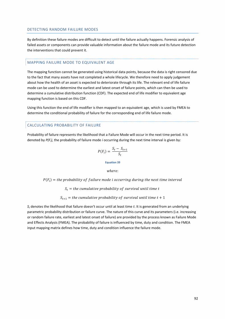
92

DETECTING RANDOM FAILURE MODES

By definition these failure modes are difficult to detect until the failure actually happens. Forensic analysis of

failed assets or components can provide valuable information about the failure mode and its future detection

the interventions that could prevent it.

MAPPING FAILURE MODE TO EQUIVALENT AGE

The mapping function cannot be generated using historical data points, because the data is right censored due

to the fact that many assets have not completed a whole lifecycle. We therefore need to apply judgement

about how the health of an asset is expected to deteriorate through its life. The relevant end of life failure

mode can be used to determine the earliest and latest onset of failure points, which can then be used to

determine a cumulative distribution function (CDF). The expected end of life modifier to equivalent age

mapping function is based on this CDF.

Using this function the end of life modifier is then mapped to an equivalent age, which is used by FMEA to

determine the conditional probability of failure for the corresponding end of life failure mode.

CALCULATING PROBABILITY OF FAILURE

Probability of failure represents the likelihood that a Failure Mode will occur in the next time period. It is

denoted by P(Fi), the probability of failure mode i occurring during the next time interval is given by:

𝑃(𝐹𝑖) = 𝑆𝑡 − 𝑆𝑡+1

𝑆𝑡

Equation 39


𝑃(𝐹𝑖) = 𝑡ℎ𝑒 𝑝𝑟𝑜𝑏𝑎𝑏𝑖𝑙𝑖𝑡𝑦 𝑜𝑓 𝑓𝑎𝑖𝑙𝑢𝑟𝑒 𝑚𝑜𝑑𝑒 𝑖 𝑜𝑐𝑐𝑢𝑟𝑟𝑖𝑛𝑔 𝑑𝑢𝑟𝑖𝑛𝑔 𝑡ℎ𝑒 𝑛𝑒𝑥𝑡 𝑡𝑖𝑚𝑒 𝑖𝑛𝑡𝑒𝑟𝑣𝑎𝑙

𝑆𝑡 = 𝑡ℎ𝑒 𝑐𝑢𝑚𝑢𝑙𝑎𝑡𝑖𝑣𝑒 𝑝𝑟𝑜𝑏𝑎𝑏𝑖𝑙𝑖𝑡𝑦 𝑜𝑓 𝑠𝑢𝑟𝑣𝑖𝑣𝑎𝑙 𝑢𝑛𝑡𝑖𝑙 𝑡𝑖𝑚𝑒 𝑡

𝑆𝑡+1 = 𝑡ℎ𝑒 𝑐𝑢𝑚𝑢𝑙𝑎𝑡𝑖𝑣𝑒 𝑝𝑟𝑜𝑏𝑎𝑏𝑖𝑙𝑖𝑡𝑦 𝑜𝑓 𝑠𝑢𝑟𝑣𝑖𝑣𝑎𝑙 𝑢𝑛𝑡𝑖𝑙 𝑡𝑖𝑚𝑒 𝑡 + 1

St denotes the likelihood that failure doesn't occur until at least time t. It is generated from an underlying

parametric probability distribution or failure curve. The nature of this curve and its parameters (i.e. increasing

or random failure rate, earliest and latest onset of failure) are provided by the process known as Failure Mode

and Effects Analysis (FMEA). The probability of failure is influenced by time, duty and condition. The FMEA

input mapping matrix defines how time, duty and condition influence the failure mode.

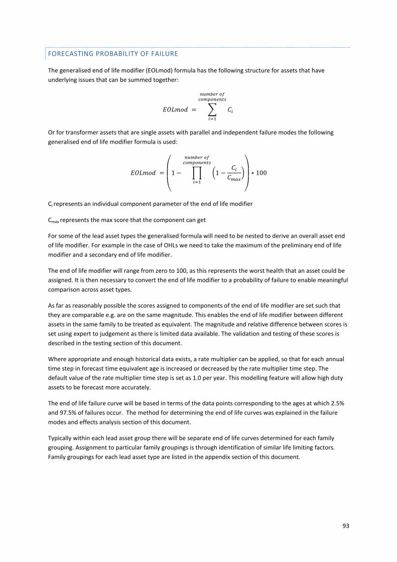
93

FORECASTING PROBABILITY OF FAILURE

The generalised end of life modifier (EOLmod) formula has the following structure for assets that have

underlying issues that can be summed together:

𝐸𝑂𝐿𝑚𝑜𝑑 = ∑ 𝐶𝑖

𝑛𝑢𝑚𝑏𝑒𝑟 𝑜𝑓𝑐𝑜𝑚𝑝𝑜𝑛𝑒𝑛𝑡𝑠

𝑖=1

Or for transformer assets that are single assets with parallel and independent failure modes the following

generalised end of life modifier formula is used:

𝐸𝑂𝐿𝑚𝑜𝑑 =

(

1 − ∏ (1 −

𝐶𝑖𝐶𝑚𝑎𝑥

)

𝑛𝑢𝑚𝑏𝑒𝑟 𝑜𝑓𝑐𝑜𝑚𝑝𝑜𝑛𝑒𝑛𝑡𝑠

𝑖=1

)

∗ 100

Ci represents an individual component parameter of the end of life modifier

Cmax represents the max score that the component can get

For some of the lead asset types the generalised formula will need to be nested to derive an overall asset end

of life modifier. For example in the case of OHLs we need to take the maximum of the preliminary end of life

modifier and a secondary end of life modifier.

The end of life modifier will range from zero to 100, as this represents the worst health that an asset could be

assigned. It is then necessary to convert the end of life modifier to a probability of failure to enable meaningful

comparison across asset types.

As far as reasonably possible the scores assigned to components of the end of life modifier are set such that

they are comparable e.g. are on the same magnitude. This enables the end of life modifier between different

assets in the same family to be treated as equivalent. The magnitude and relative difference between scores is

set using expert to judgement as there is limited data available. The validation and testing of these scores is

described in the testing section of this document.

Where appropriate and enough historical data exists, a rate multiplier can be applied, so that for each annual

time step in forecast time equivalent age is increased or decreased by the rate multiplier time step. The

default value of the rate multiplier time step is set as 1.0 per year. This modelling feature will allow high duty

assets to be forecast more accurately.

The end of life failure curve will be based in terms of the data points corresponding to the ages at which 2.5%

and 97.5% of failures occur. The method for determining the end of life curves was explained in the failure

modes and effects analysis section of this document.

Typically within each lead asset group there will be separate end of life curves determined for each family

grouping. Assignment to particular family groupings is through identification of similar life limiting factors.

Family groupings for each lead asset type are listed in the appendix section of this document.

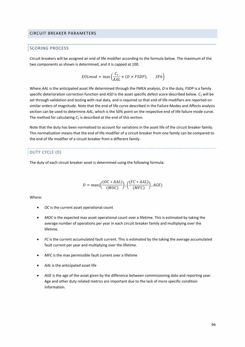
94

CIRCUIT BREAKER PARAMETERS

SCORING PROCESS

Circuit breakers will be assigned an end of life modifier according to the formula below. The maximum of the

two components as shown is determined, and it is capped at 100.

𝐸𝑂𝐿𝑚𝑜𝑑 = max (𝐶1𝐴𝐴𝐿

× (𝐷 × 𝐹𝑆𝐷𝑃), 𝑆𝐹6)

Where AAL is the anticipated asset life determined through the FMEA analysis, D is the duty, FSDP is a family

specific deterioration correction function and ASD is the asset specific defect score described below. C1 will be

set through validation and testing with real data, and is required so that end of life modifiers are reported on

similar orders of magnitude. Note that the end of life curve described in the Failure Modes and Affects analysis

section can be used to determine AAL, which is the 50% point on the respective end of life failure mode curve.

The method for calculating C1 is described at the end of this section.

Note that the duty has been normalised to account for variations in the asset life of the circuit breaker family.

This normalisation means that the end of life modifier of a circuit breaker from one family can be compared to

the end of life modifier of a circuit breaker from a different family.

DUTY CYCLE (D)

The duty of each circuit breaker asset is determined using the following formula:

𝐷 = max (((𝑂𝐶 ∗ 𝐴𝐴𝐿)

(𝑀𝑂𝐶)) , (

(𝐹𝐶 ∗ 𝐴𝐴𝐿)

(𝑀𝐹𝐶)) , 𝐴𝐺𝐸)

Where:

OC is the current asset operational count

MOC is the expected max asset operational count over a lifetime. This is estimated by taking the

average number of operations per year in each circuit breaker family and multiplying over the

lifetime.

FC is the current accumulated fault current. This is estimated by the taking the average accumulated

fault current per year and multiplying over the lifetime.

MFC is the max permissible fault current over a lifetime

AAL is the anticipated asset life

AGE is the age of the asset given by the difference between commissioning date and reporting year.

Age and other duty related metrics are important due to the lack of more specific condition

information.

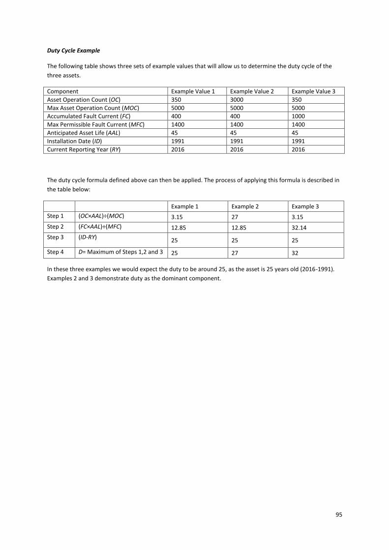
95

Duty Cycle Example

The following table shows three sets of example values that will allow us to determine the duty cycle of the

three assets.

Component Example Value 1 Example Value 2 Example Value 3

Asset Operation Count (OC) 350 3000 350

Max Asset Operation Count (MOC) 5000 5000 5000

Accumulated Fault Current (FC) 400 400 1000

Max Permissible Fault Current (MFC) 1400 1400 1400

Anticipated Asset Life (AAL) 45 45 45

Installation Date (ID) 1991 1991 1991

Current Reporting Year (RY) 2016 2016 2016

The duty cycle formula defined above can then be applied. The process of applying this formula is described in

the table below:

Example 1 Example 2 Example 3

Step 1 (OC×AAL)÷(MOC) 3.15 27 3.15

Step 2 (FC×AAL)÷(MFC) 12.85 12.85 32.14

Step 3 (ID-RY) 25 25 25

Step 4 D= Maximum of Steps 1,2 and 3 25 27 32

In these three examples we would expect the duty to be around 25, as the asset is 25 years old (2016-1991).

Examples 2 and 3 demonstrate duty as the dominant component.

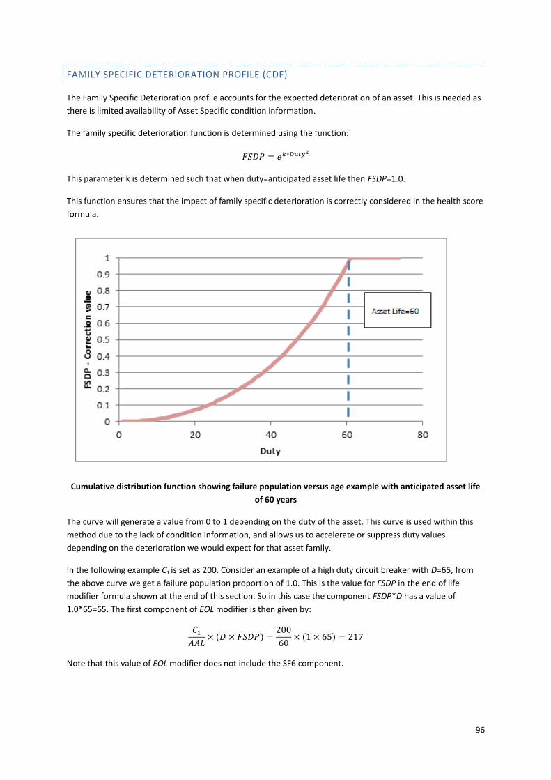
96

FAMILY SPECIFIC DETERIORATION PROFILE (CDF)

The Family Specific Deterioration profile accounts for the expected deterioration of an asset. This is needed as

there is limited availability of Asset Specific condition information.

The family specific deterioration function is determined using the function:

𝐹𝑆𝐷𝑃 = 𝑒𝑘∗𝐷𝑢𝑡𝑦2

This parameter k is determined such that when duty=anticipated asset life then FSDP=1.0.

This function ensures that the impact of family specific deterioration is correctly considered in the health score

formula.

Cumulative distribution function showing failure population versus age example with anticipated asset life

of 60 years

The curve will generate a value from 0 to 1 depending on the duty of the asset. This curve is used within this

method due to the lack of condition information, and allows us to accelerate or suppress duty values

depending on the deterioration we would expect for that asset family.

In the following example C1 is set as 200. Consider an example of a high duty circuit breaker with D=65, from

the above curve we get a failure population proportion of 1.0. This is the value for FSDP in the end of life

modifier formula shown at the end of this section. So in this case the component FSDP*D has a value of

1.0*65=65. The first component of EOL modifier is then given by:

𝐶1𝐴𝐴𝐿

× (𝐷 × 𝐹𝑆𝐷𝑃) =200

60× (1 × 65) = 217

Note that this value of EOL modifier does not include the SF6 component.

97

SF6 COMPONENT OF ASD (SF6)

The SF6 component of the end of life modifier is a binary score, which means it can only have one of two

values, and will force the end of life modifier to a high value in the event of a significant leakage of SF6.

Significant leakage is deemed to have occurred when either of the following conditions is satisfied.

If

𝐴𝑛𝑛𝑢𝑎𝑙 𝐴𝑠𝑠𝑒𝑡 𝑆𝐹6 𝑅𝑒𝑝𝑜𝑟𝑡𝑎𝑏𝑙𝑒 𝐿𝑒𝑎𝑘𝑎𝑔𝑒

𝐴𝑠𝑠𝑒𝑡 𝑆𝐹6 𝐼𝑛𝑣𝑒𝑛𝑡𝑜𝑟𝑦 ≥ 5%

Or

𝐴𝑛𝑛𝑢𝑎𝑙 𝐴𝑠𝑠𝑒𝑡 𝑆𝐹6 𝑅𝑒𝑝𝑜𝑟𝑡𝑎𝑏𝑙𝑒 𝐿𝑒𝑎𝑘𝑎𝑔𝑒 > 10𝐾𝑔

Then SF6 = 100.

Else SF6 = 0

Asset SF6 Reportable Leakage is the quantity (in kg) of SF6 leakage since the last repair up to a maximum of

one year ago. Asset SF6 Inventory is the Reported volume of SF6. The expected leakage is small compared to

the threshold values and so does not need to be considered explicitly within the above formulation.

The pressure equipment directive specifies allowed leakage of SF6 per annum, so is already factored into the

above equations.

SF6 is a greenhouse gas covered by The Fluorinated Greenhouse Gases Regulations 2015, which places

significant limits on permitted Leakage.

1. Operators of equipment that contains fluorinated greenhouse gases shall take precautions to prevent the

unintentional release (‘leakage’) of those gases. They shall take all measures which are technically and

economically feasible to minimise leakage of fluorinated greenhouse gases.

2. Where a leakage of fluorinated greenhouse gases is detected, the operators shall ensure that the equipment

is repaired without undue delay. (Chapter 2 Article 3 Sections 2 and 3 from http://eur-lex.europa.eu/legal-

content/EN/TXT/PDF/?uri=CELEX:32014R0517&from=EN)

A high score has been applied for SF6 to account for these regulations, such that significant SF6 leakage will

result in an immediate requirement for intervention.

Example calculation of SF6 component

Example 1 Example 2 Example 3

Annual Asset SF6 Reportable Leakage(kg) 4 9 100

Asset SF6 Inventory(kg) 120 120 2400

Annual Leak Rate % 3.3% 7.5% 4.2%

Score Impact 0 100 100

http://eur-lex.europa.eu/legal-content/EN/TXT/PDF/?uri=CELEX:32014R0517&from=EN

http://eur-lex.europa.eu/legal-content/EN/TXT/PDF/?uri=CELEX:32014R0517&from=EN

98

Procedure for determining C1,

The following steps describe the process for setting C1 . This will be performed once before implementing the

methodology and will not need to be done on a recurring basis:

1) Determine the value of 1/AAL*(D*FSDP) for each year for all circuit breaker lead assets. In general it is

expected that this value will range between 0 and 2.

2) Determine the 95th percentile value from the ordered distribution of these values. The 95th

percentile has

been chosen to ignore outliers. Call this value V95

3) The end of life modifier is an integer with no upper limit. To give enough resolution we need the end of life

modifiers to generally be in the range 0-100. Therefore:

C1= 100/V95

C1 can then be rounded to 1dp

It is acknowledged that the method described is similar to an aged based asset management approach,

however additional condition information relating to number of operations, fault current and SF6 is being

utilised where possible.

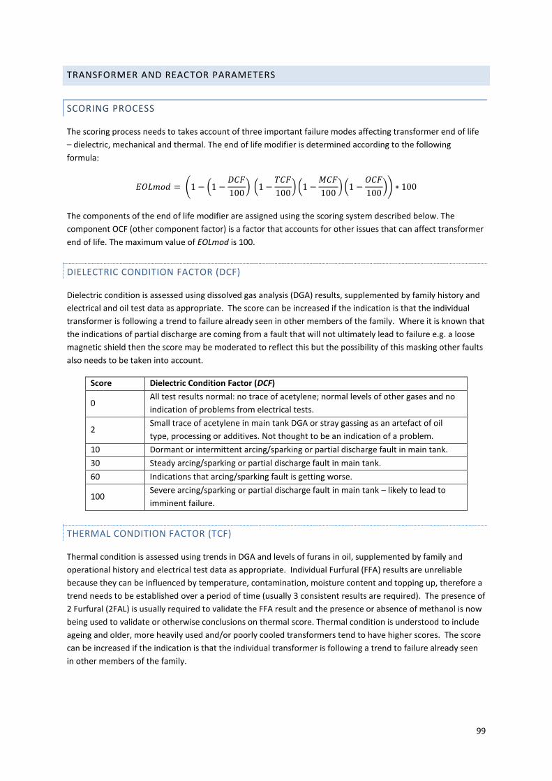
99

TRANSFORMER AND REACTOR PARAMETERS

SCORING PROCESS

The scoring process needs to takes account of three important failure modes affecting transformer end of life

– dielectric, mechanical and thermal. The end of life modifier is determined according to the following

formula:

𝐸𝑂𝐿𝑚𝑜𝑑 = (1 − (1 −𝐷𝐶𝐹

100) (1 −

𝑇𝐶𝐹

100) (1 −

𝑀𝐶𝐹

100) (1 −

𝑂𝐶𝐹

100)) ∗ 100

The components of the end of life modifier are assigned using the scoring system described below. The

component OCF (other component factor) is a factor that accounts for other issues that can affect transformer

end of life. The maximum value of EOLmod is 100.

DIELECTRIC CONDITION FACTOR (DCF)

Dielectric condition is assessed using dissolved gas analysis (DGA) results, supplemented by family history and

electrical and oil test data as appropriate. The score can be increased if the indication is that the individual

transformer is following a trend to failure already seen in other members of the family. Where it is known that

the indications of partial discharge are coming from a fault that will not ultimately lead to failure e.g. a loose

magnetic shield then the score may be moderated to reflect this but the possibility of this masking other faults

also needs to be taken into account.

Score Dielectric Condition Factor (DCF)

0 All test results normal: no trace of acetylene; normal levels of other gases and no

indication of problems from electrical tests.

2 Small trace of acetylene in main tank DGA or stray gassing as an artefact of oil

type, processing or additives. Not thought to be an indication of a problem.

10 Dormant or intermittent arcing/sparking or partial discharge fault in main tank.

30 Steady arcing/sparking or partial discharge fault in main tank.

60 Indications that arcing/sparking fault is getting worse.

100 Severe arcing/sparking or partial discharge fault in main tank – likely to lead to

imminent failure.

THERMAL CONDITION FACTOR (TCF)

Thermal condition is assessed using trends in DGA and levels of furans in oil, supplemented by family and

operational history and electrical test data as appropriate. Individual Furfural (FFA) results are unreliable

because they can be influenced by temperature, contamination, moisture content and topping up, therefore a

trend needs to be established over a period of time (usually 3 consistent results are required). The presence of

2 Furfural (2FAL) is usually required to validate the FFA result and the presence or absence of methanol is now

being used to validate or otherwise conclusions on thermal score. Thermal condition is understood to include

ageing and older, more heavily used and/or poorly cooled transformers tend to have higher scores. The score

can be increased if the indication is that the individual transformer is following a trend to failure already seen

in other members of the family.

100

Score Thermal Condition Factor (TCF)

0

No signs of ageing including no credible furans >0.10ppm and methanol

≤0.05ppm.

The credibility of furan results usually depends on the presence of 2 Furfural

(2FAL).

2

Diagnostic markers exist that could indicate ageing (including credible furans in

the range 0.10-0.50ppm) but are either not showing a credible progression or are

thought to be the result of contamination.

The credibility of furan results usually depends on the presence of 2 Furfural

(2FAL).

10

Indications or expectations that the transformer is reaching or has reached mid-

life for example: credible furans in the range 0.51-1.00ppm or stable furans >1ppm

possibly as a result of historic ageing.

and/or

Raised levels of methane or ethane in main tank DGA consistent with low

temperature overheating.

and/or

Transformers with diagnostic markers resulting from oil contamination (e.g.

furans, specifically 2FAL) that may mask signs of ageing.

30

Moderate ageing for example: credible furans consistently > 1ppm with a clear

upward trend.

and/or

Significant overheating fault (steadily rising trend of ethylene in main tank DGA).

60

Advanced ageing for example: credible furans > 1.5ppm showing a clear upward

trend or following the indications of a sister unit found to be severely aged when

scrapped.

and/or

Indications of a worsening overheating fault.

100

Very advanced ageing for example: credible furans >2ppm with an upward trend

or following the indications of a sister unit found to be severely aged when

scrapped.

and/or

Serious overheating fault.

Electrical test data may be used to support a higher thermal score where they show poor insulation condition

however experience shows that not all poor thermal conditions can be detected by electrical tests.

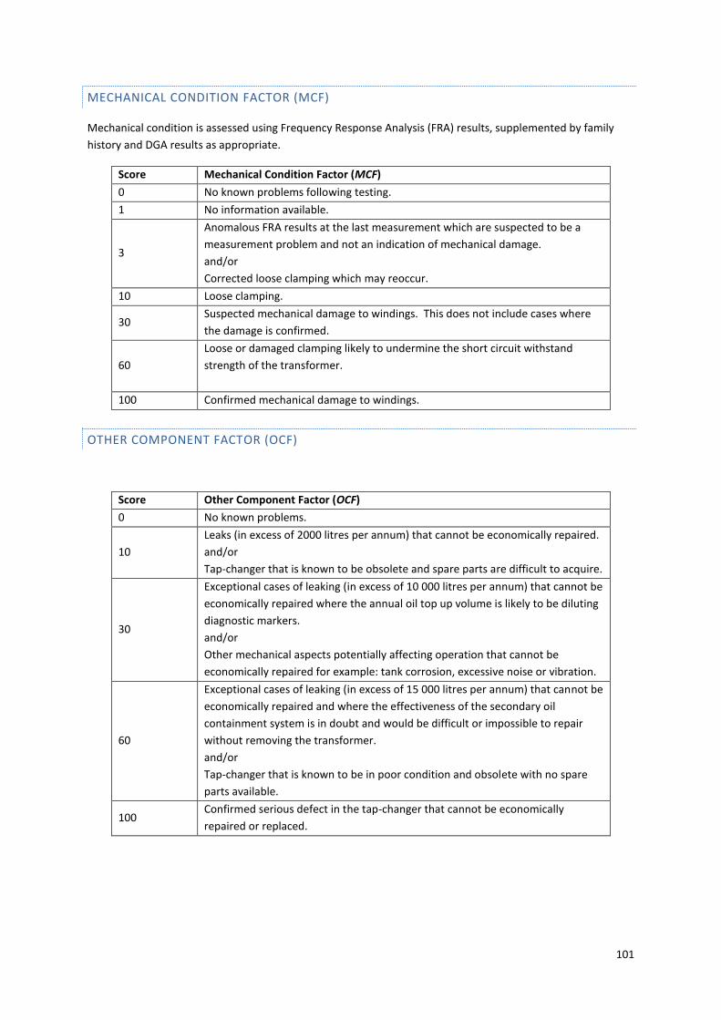
101

MECHANICAL CONDITION FACTOR (MCF)

Mechanical condition is assessed using Frequency Response Analysis (FRA) results, supplemented by family

history and DGA results as appropriate.

Score Mechanical Condition Factor (MCF)

0 No known problems following testing.

1 No information available.

3

Anomalous FRA results at the last measurement which are suspected to be a

measurement problem and not an indication of mechanical damage.

and/or

Corrected loose clamping which may reoccur.

10 Loose clamping.

30 Suspected mechanical damage to windings. This does not include cases where

the damage is confirmed.

60

Loose or damaged clamping likely to undermine the short circuit withstand

strength of the transformer.

100 Confirmed mechanical damage to windings.

OTHER COMPONENT FACTOR (OCF)

Score Other Component Factor (OCF)

0 No known problems.

10

Leaks (in excess of 2000 litres per annum) that cannot be economically repaired.

and/or

Tap-changer that is known to be obsolete and spare parts are difficult to acquire.

30

Exceptional cases of leaking (in excess of 10 000 litres per annum) that cannot be

economically repaired where the annual oil top up volume is likely to be diluting

diagnostic markers.

and/or

Other mechanical aspects potentially affecting operation that cannot be

economically repaired for example: tank corrosion, excessive noise or vibration.

60

Exceptional cases of leaking (in excess of 15 000 litres per annum) that cannot be

economically repaired and where the effectiveness of the secondary oil

containment system is in doubt and would be difficult or impossible to repair

without removing the transformer.

and/or

Tap-changer that is known to be in poor condition and obsolete with no spare

parts available.

100 Confirmed serious defect in the tap-changer that cannot be economically

repaired or replaced.

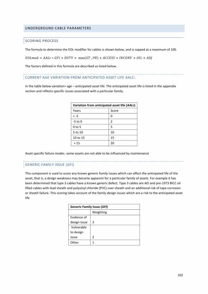
102

UNDERGROUND CABLE PARAMETERS

SCORING PROCESS

The formula to determine the EOL modifier for cables is shown below, and is capped at a maximum of 100.

𝐸𝑂𝐿𝑚𝑜𝑑 = 𝐴𝐴𝐿𝑐 ∗ 𝐺𝐹𝐼 + 𝐷𝑈𝑇𝑌 + max(𝐺𝑇 , 𝑃𝑅) + 𝐴𝐶𝐶𝐸𝑆𝑆 + 𝐼𝑁𝐶𝑂𝑁𝑉 + 𝑂𝐼𝐿 + 𝐴𝐷𝐽

The factors defined in this formula are described as listed below.

CURRENT AGE VARIATION FROM ANTICIPATED ASSET LIFE AALC:

In the table below variation= age – anticipated asset life. The anticipated asset life is listed in the appendix

section and reflects specific issues associated with a particular family.

Asset specific failure modes -some assets are not able to be influenced by maintenance

GENERIC FAMILY ISSUE (GFI)

This component is used to score any known generic family issues which can affect the anticipated life of the

asset, that is, a design weakness may become apparent for a particular family of assets. For example it has

been determined that type 3 cables have a known generic defect. Type 3 cables are AEI and pre-1973 BICC oil

filled cables with lead sheath and polyvinyl chloride (PVC) over sheath and an additional risk of tape corrosion

or sheath failure. This scoring takes account of the family design issues which are a risk to the anticipated asset

life

Generic Family Issue (GFI)

Weighting

Evidence of

design issue 3

Vulnerable

to design

issue 2

Other 1

Variation from anticipated asset life (AALc)

Years Score

< -5 0

-5 to 0 2

0 to 5 5

5 to 10 10

10 to 15 15

> 15 20

103

DUTY (DUTY)

This represents the operational stress that a cable route has undergone during the last 5 years. It is measured

in terms of the hours the cable has operated at or above its maximum designed rating during the last 5 years.

The England and Wales transmission owner will set this factor to zero, as cables are not operated at or even

near maximum designed rating.

Duty – hours at or above max rating (DUTY)

> Hours Score

0 0

24 5

48 10

120 15

GRAND TOTAL COST OF DEFECT AND FAULT REPAIRS OVER THE LAST TEN YEARS SCORE 0-

60 (GT)

This metric is the total cost associated with defect and fault repair summed over the last 10 years across entire

cable route. This does not include routine activates unless it can be demonstrated that they are due to the

poor condition of the cable. Repairs are expected to be undertaken following faults, forced or planned

outages.

Grand total - Last Ten years (GT)

> £ Score

£0 0

£500,000 2

£1,000,000 10

£2,000,000 20

£3,000,000 40

£4,000,000 50

£5,000,000 60

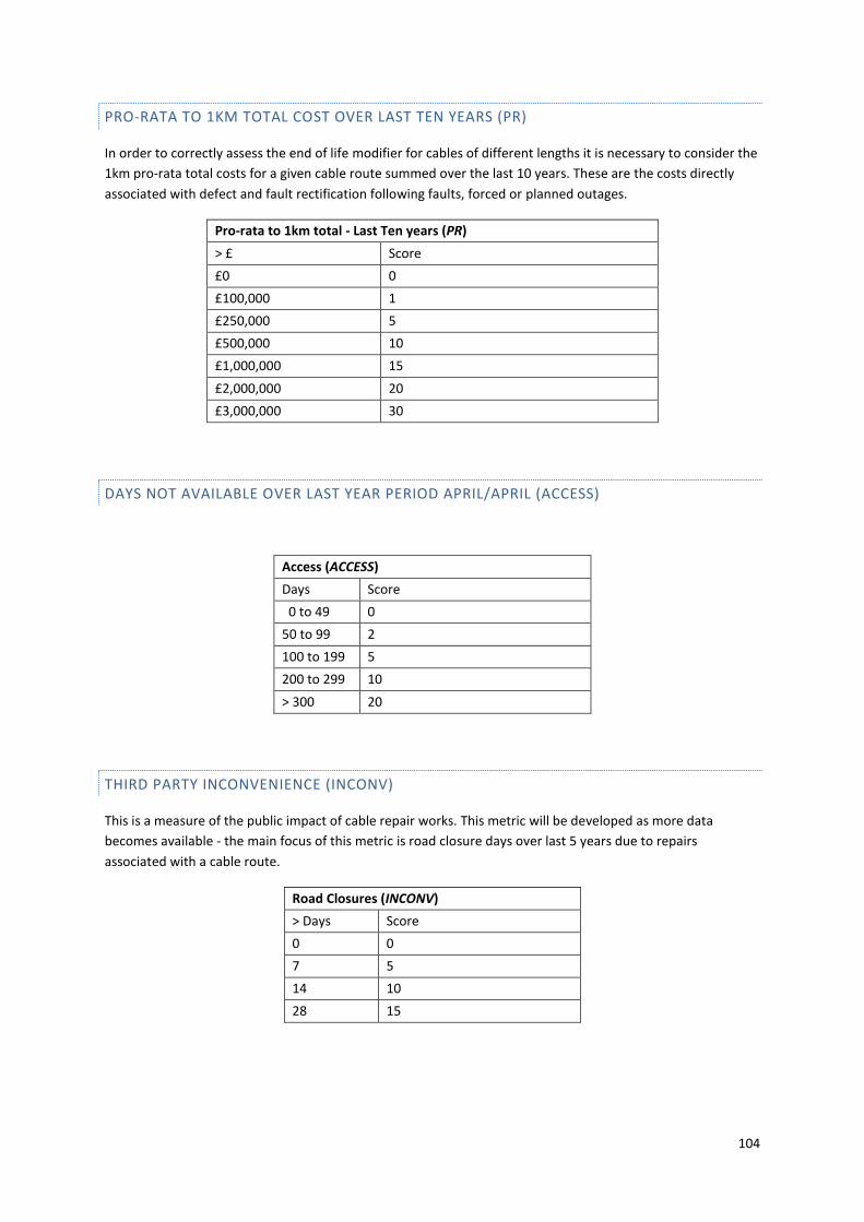
104

PRO-RATA TO 1KM TOTAL COST OVER LAST TEN YEARS (PR)

In order to correctly assess the end of life modifier for cables of different lengths it is necessary to consider the

1km pro-rata total costs for a given cable route summed over the last 10 years. These are the costs directly

associated with defect and fault rectification following faults, forced or planned outages.

Pro-rata to 1km total - Last Ten years (PR)

> £ Score

£0 0

£100,000 1

£250,000 5

£500,000 10

£1,000,000 15

£2,000,000 20

£3,000,000 30

DAYS NOT AVAILABLE OVER LAST YEAR PERIOD APRIL/APRIL (ACCESS)

Access (ACCESS)

Days Score

0 to 49 0

50 to 99 2

100 to 199 5

200 to 299 10

> 300 20

THIRD PARTY INCONVENIENCE (INCONV)

This is a measure of the public impact of cable repair works. This metric will be developed as more data

becomes available - the main focus of this metric is road closure days over last 5 years due to repairs

associated with a cable route.

Road Closures (INCONV)

> Days Score

0 0

7 5

14 10

28 15

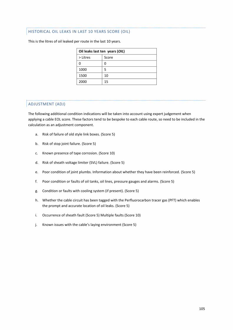
105

HISTORICAL OIL LEAKS IN LAST 10 YEARS SCORE (OIL)

This is the litres of oil leaked per route in the last 10 years.

Oil leaks last ten years (OIL)

> Litres Score

0 0

1000 5

1500 10

2000 15

ADJUSTMENT (ADJ)

The following additional condition indications will be taken into account using expert judgement when

applying a cable EOL score. These factors tend to be bespoke to each cable route, so need to be included in the

calculation as an adjustment component.

a. Risk of failure of old style link boxes. (Score 5)

b. Risk of stop joint failure. (Score 5)

c. Known presence of tape corrosion. (Score 10)

d. Risk of sheath voltage limiter (SVL) failure. (Score 5)

e. Poor condition of joint plumbs. Information about whether they have been reinforced. (Score 5)

f. Poor condition or faults of oil tanks, oil lines, pressure gauges and alarms. (Score 5)

g. Condition or faults with cooling system (if present). (Score 5)

h. Whether the cable circuit has been tagged with the Perfluorocarbon tracer gas (PFT) which enables

the prompt and accurate location of oil leaks. (Score 5)

i. Occurrence of sheath fault (Score 5) Multiple faults (Score 10)

j. Known issues with the cable’s laying environment (Score 5)

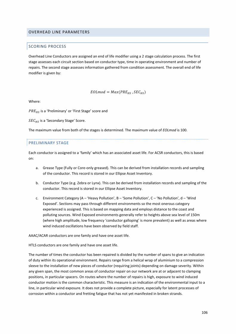
106

OVERHEAD LINE PARAMETERS

SCORING PROCESS

Overhead Line Conductors are assigned an end of life modifier using a 2 stage calculation process. The first

stage assesses each circuit section based on conductor type, time in operating environment and number of

repairs. The second stage assesses information gathered from condition assessment. The overall end of life

modifier is given by:

𝐸𝑂𝐿𝑚𝑜𝑑 = 𝑀𝑎𝑥(𝑃𝑅𝐸𝐻𝑆 , 𝑆𝐸𝐶𝐻𝑆)

Where:

𝑃𝑅𝐸𝐻𝑆 is a ‘Preliminary’ or ‘First Stage’ score and

𝑆𝐸𝐶𝐻𝑆 is a ‘Secondary Stage’ Score.

The maximum value from both of the stages is determined. The maximum value of EOLmod is 100.

PRELIMINARY STAGE

Each conductor is assigned to a ‘family’ which has an associated asset life. For ACSR conductors, this is based

on:

a. Grease Type (Fully or Core-only greased). This can be derived from installation records and sampling

of the conductor. This record is stored in our Ellipse Asset Inventory.

b. Conductor Type (e.g. Zebra or Lynx). This can be derived from installation records and sampling of the

conductor. This record is stored in our Ellipse Asset Inventory.

c. Environment Category (A – ‘Heavy Pollution’, B – ‘Some Pollution’, C – ‘No Pollution’, d – ‘Wind

Exposed’. Sections may pass through different environments so the most onerous category

experienced is assigned. This is based on mapping data and employs distance to the coast and

polluting sources. Wind Exposed environments generally refer to heights above sea level of 150m

(where high amplitude, low frequency ‘conductor galloping’ is more prevalent) as well as areas where

wind induced oscillations have been observed by field staff.

AAAC/ACAR conductors are one family and have one asset life.

HTLS conductors are one family and have one asset life.

The number of times the conductor has been repaired is divided by the number of spans to give an indication

of duty within its operational environment. Repairs range from a helical wrap of aluminium to a compression

sleeve to the installation of new pieces of conductor (requiring joints) depending on damage severity. Within

any given span, the most common areas of conductor repair on our network are at or adjacent to clamping

positions, in particular spacers. On routes where the number of repairs is high, exposure to wind induced

conductor motion is the common characteristic. This measure is an indication of the environmental input to a

line, in particular wind exposure. It does not provide a complete picture, especially for latent processes of

corrosion within a conductor and fretting fatigue that has not yet manifested in broken strands.

107

The preliminary end of life modifier is taken to be the average score produced by the conditions met below. If

the repairs component of the equation is high it always requires further investigation, regardless of the age of

the asset. The spread of repair locations is also significant. Clusters may appear on spans/ sections with local

environment characteristics (e.g. turbulence level). For example, the damping or configuration of the

conductor bundle may require intervention to prevent earlier failure of this part of the line.

Because the processes of corrosion, wear and fatigue reduce wire cross section and strength over time, ‘Age’

of a line in its respective operating environment is a significant part of the conductor assessment. Since age is

capped at a score of 35 it means that its impact on the overall value of end of life modified is limited, and

prevents it acting as a floor.

Our ability to detect all the condition states of a conductor is limited. This is a composite, linear asset where

condition states remain hidden without intrusive analysis. The act of taking a sample is time consuming

(average 3-4 days per line gang), can only be done in places where conductor can be lowered to the ground

and introduces more risk to the system by the insertion of joints between new and old conductor. As such,

where intrusive conductor condition assessment is difficult, sometimes impossible to obtain age and visual

inspection (no of repairs made to the conductor) is a proxy.

𝑃𝑅𝐸𝐻𝑆 = average(AGE, REP)

AGE Score

<=5 Years old 0

>5 Years old >=8 from anticipated life 5

<8 years>3 years from anticipated life 10

<3 years from anticipated life 20

REP= Number of conductor repairs in the span being assessed divided by the total number of spans on the

route or section.

REP: No. of Repairs/ No. of Spans Score

0 0

>0<0.2 5

>=0.2 10

>=0.4 20

>=0.6 50

SECOND STAGE

On completion of the preliminary scoring, further condition indications will be reviewed to allow a second

stage assessment of a conductor.

𝑆𝑖 = 𝐴𝐻 + 𝑉𝐴 + 𝐺𝐿 + 𝐷𝑆𝑆 + 𝐺𝑇 + 𝐶𝐿 + 𝐷𝐴𝑆 + 𝑇𝐵𝐿 + 𝑇𝑇

𝑃𝐶𝑆𝐼 = max𝐴𝑙𝑙 𝑝ℎ𝑎𝑠𝑒 𝑐𝑜𝑛𝑑𝑢𝑐𝑡𝑜𝑟 𝑠𝑎𝑚𝑝𝑙𝑒𝑠 (𝑆1, 𝑆2, 𝑆3…𝑆𝑛 )

𝑆𝐸𝐶𝐻𝑆 = 𝑚𝑎𝑥(𝑃𝐶𝑆𝐼, 𝐶𝑂𝑅) * VAL

The PCSI component is therefore determined by adding up the component scores for each phase conductor

sample (Si). This generates a total result for each phase conductor sample. The maximum total result across all

phase conductor samples then gives the value if PCSI.

This second stage assessment is the maximum of either PCSI or non-intrusive core corrosion surveys.

108

A phase conductor sample requires a conductor to be lowered to the ground, where typically, a length is taken

from the anchor clamp to the first ‘spacer clamp’ in the span. The test is destructive, this is cut out and then a

new piece of conductor jointed in. The spacer clamp area is a corrosion, wear and fatigue location where the

worst conductor degradation is usually witnessed. Other locations of interest within a conductor span are the

area around a suspension shoe, dampers, any other clamping device and the bottom of the wire catenary.

Phase Conductor Sampling Interpretation (out of 100)

𝐴𝐻 + 𝑉𝐴 + 𝐺𝐿 + 𝐷𝑆𝑆 + 𝐺𝑇 + 𝐶𝐿 + 𝐷𝐴𝑆 + 𝑇𝐵𝐿+ 𝑇𝑇

Presence of Aluminium Hydroxide (a corrosion product) (AH) (0-15)

Significant – Area/Areas with full surface coverage of powder.

15

Present – Area/Areas with small clusters of powder or a small number of particles scattered over surface

10

None 0

Visual Assessment of Steel Core Galvanising (VA) (0-15)

Loss – 10% + galvanising is missing/damaged 15

Small Loss – small areas of (no more that 10% of damaged/ missing galvanising

10

Good – Galvanising appears intact 0

Grease Level and Quality (GL) (0-10)

Core Only Greased Dry 10

Core Only Greased Flexible 5

Fully Greased Dry 2.5

Fully Greased Flexible 0

Diameter of Steel Strands (DSS) (0-5)

Less than 0%, or lower than the Min Spec of 3.18mm 5

Between 0 and 0.4 % (inclusive) Min Spec of 3.18mm 2.5

Greater than 0.4 % Min Spec of 3.18mm 0

Measurement of Galvanising Thickness on Outer and Inner Face of Steel Core Wire (GT) (0-5)

Average <20 microns 5

Average >=20 microns 2

Average >=49 microns 0

Measurement of Corrosion Layer of Outer and Inner Face of Aluminium Strands (CL) (0-5)

Average >=275 5

Average >100 2

Average >0 0

Diameter of Aluminium Strands (DAS) (0-5)

Average >=275 5

Average >100 2

Average >0 0

Average Tensile Breaking Load of Outer Aluminium Strands (TBL) (0-20)

<1120N 20

>=1120N 15

>=1280N 10

>=1310N 0

Torsion Test (Average Revolutions to Failure of Outer Aluminium Strands (TT) (0-20)

<1 revolution to failure 20

>=1 revolution to failure 15

>=10 revolutions to failure 5

>=18 revolutions to failure 0

109

Eddy current non-intrusive core corrosion surveys measure the residual zinc coating of the steel core within

ACSR. These employ a device that is required to be mounted on and propelled down a conductor wire.

Changes in magnetic flux density detect loss of zinc and aluminium to the steel core.

Core Sample Interpretation Score (COR)

Residual zinc coating of 5 microns or less (‘Severe Corrosion’)

50

Minimum 0

VALIDITY MULTIPLIER

To aim for condition data that is indicative of the whole circuit or section being assessed, a validity criterion is

applied. All environment categories the circuit passes through must be assessed and at least one conductor

sample per 50km is required.

Results of the Second Stage element are only considered if the criterion for a ‘valid’ set of condition

assessments described above is met. Note that a zero value of VAL implies that there is not enough condition

information and since the end of life modifier formula takes the maximum of the preliminary and secondary

components this is valid.

𝑉𝐴𝐿 = 𝐶𝑟𝑖𝑡𝑒𝑟𝑖𝑎 𝐴 ∗ 𝐶𝑟𝑖𝑡𝑒𝑟𝑖𝑎 𝐵

Validity Criteria A Criteria A value

No. of Environment Categories/No. of Categories Assessed = 1

1

No. of Environment Categories/No. of Categories Assessed <1

0

Validity Criteria B Criteria B value

No. of samples per 50 route km >=1 1

No. of samples per 50 route km <1 0

OVERALL CONDUCTOR SCORE

The end of life modifier is given by the following formula:

𝐸𝑂𝐿𝑚𝑜𝑑 = 𝑚𝑎𝑥(𝑃𝑅𝐸𝐻𝑆 , 𝑆𝐸𝐶𝐻𝑆 )

where

𝑃𝑅𝐸𝐻𝑆 = max(AGE, REP)

𝑆𝐸𝐶𝐻𝑆 = 𝑚𝑎𝑥(𝑃𝐶𝑆𝐼, 𝐶𝑂𝑅) * VAL

𝑃𝐶𝑆𝐼 = max𝐴𝑙𝑙 𝑝ℎ𝑎𝑠𝑒 𝑐𝑜𝑛𝑑𝑢𝑐𝑡𝑜𝑟 𝑠𝑎𝑚𝑝𝑙𝑒𝑠 (𝑆1, 𝑆2, 𝑆3…𝑆𝑛 )

𝑆𝑖 = 𝐴𝐻 + 𝑉𝐴 + 𝐺𝐿 + 𝐷𝑆𝑆 + 𝐺𝑇 + 𝐶𝐿 + 𝐷𝐴𝑆 + 𝑇𝐵𝐿 + 𝑇𝑇

110

FITTINGS

Overhead Line Fittings are assigned a HS using a 3 stage calculation process. The first stage is preliminary

assessment based on age. The second stage is a visual condition assessment (referred to as a ‘Level 1’) and the

third stage is an ‘outage’ or intrusive condition assessment (‘Level 2’).

Scoring assessments are made on sections of circuit that are typically homogenous in conductor type,

installation date and environment.

OHL FITTINGS END OF LIFE MODIFIER

The formula to determine the EOL modifier of fittings is given below, and is capped at a maximum of 100.

𝐸𝑂𝐿𝑚𝑜𝑑 =max(𝑆𝑃𝐴, 𝐷𝐴𝑀, 𝐼𝑁𝑆, 𝑃𝐻𝐹) + 𝐸𝑁𝑉𝑊𝐼𝑀 + 𝐸𝑁𝑉𝑃𝑂𝐿

6

The components of this formula will all be broken down and described in more detail below. The meaning of

these components is:

1. Spacers (SPA)

2. Dampers (DAM)

3. Insulators (INS)

4. Phase Fittings (PHF). This category includes linkages (shackles, straps, dowel pins etc.) and Arcing

Horns/Corona Rings.

Environmental factors have an impact on the assessment of fittings. These are indicators of the level of

mechanical duty and chemical attack that OHL fittings systems undergo.

1. Wind Induced Motion (WIM)

2. Pollution (POL)

This is then averaged out across a circuit for each component class (spacers, dampers, insulators and phase

fittings), so it remains is necessary to review the results per tower/span to understand the distribution of

condition statements across the system. A targeted intervention may be required within a component class or

within a sub section of the OHL circuit or both.

This is a likely outcome as fittings systems within older OHL assets display greater diversity in component types

and condition because of previous repairs and targeted interventions to manage defects.

111

PRELIMINARY ASSESSMENT

The Preliminary assessment of spacers, dampers, insulators and phase fittings is based on the age of the oldest

components versus the anticipated life. The preliminary score for each of these components (𝑆𝑃𝐴𝑃𝑅𝐸 ,

𝐷𝐴𝑀𝑃𝑅𝐸 , 𝐼𝑁𝑆𝑃𝑅𝐸 , 𝑃𝐻𝑆𝑃𝑅𝐸 ) can be determined from the table below.

Assessment of Spacers, Dampers, Insulators and Phase Fittings

Score

>=13 years from anticipated life 0




LEVEL 1 AND LEVEL 2 CONDITION ASSESSMENT

Each of the categories, spacers, dampers, insulators and phase fittings are assessed against condition

statements. Each of these statements has a weighting which results in the overall End of Life modifier.

Level 1 is a visual condition assessment of fittings components. The usual method of data collection is by High

Definition Camera mounted to a helicopter.

Level 2 is an ‘outage’ or ‘intrusive’ condition assessment. This extra degree of inspection is required on those

components likely to produce ‘false negative’ or ‘false positive’ results when the level 1 approach is adopted.

This includes wear to phase fittings and loss of dielectric strength in insulation. Only some of the components

have level 2 information.

SPACERS

𝑆𝑃𝐴 = (𝑆𝑃𝐴𝑃𝑅𝐸 ∗ 𝐿𝑉𝐿1) + 𝑆𝑃𝐴𝐹𝐴𝑀 + 𝑆𝑃𝐴𝐿𝑉𝐿1

Where:

SPA is the overall spacer score

𝑆𝑃𝐴𝑃𝑅𝐸 is the preliminary spacer score

LVL1 is a multiplier: if Level 1 condition assessment is available (=0), if Level 1 condition assessment is not

available (=1)

𝑆𝑃𝐴𝐹𝐴𝑀 is the spacer family score

𝑆𝑃𝐴𝐿𝑉𝐿1 is the Level 1 Condition Assessment score for spacers.

There is no Level 2 stage assessment for Spacers

112

Spacer Family 𝑺𝑷𝑨𝑭𝑨𝑴 Score

Phase Quad and Twin Semi-Flexible – Andre, BICC, Bowthorpe, Delta Enfield, Metalastik. 200

Phase Quad Semi-Flexible – Hydro Quebec. 0

Phase Quad and Triple Semi-Flexible, Key-Installed – PLP, Dulmison, Mosdorfer. 0

Phase Twin Rigid, Key-Installed – PLP, Dulmison, Mosdorfer. 0

Phase Quad, Twin and Triple Spacer Damper – PLP, Dulmison, Mosdorfer. 0

Jumper and Downlead Quad, Twin and Triple Rigid Spacers – Andre, Metalastik, PLP, TYCO, Bonded and Compression types.

0

Spacer Visual Condition Statements Score

(=1)(Good Condition)(Tight and Secure) 0

(2)(Dull Appearance)(Tight and secure) 0

(3)(Black appearance)(Tight and Secure) 0

(6)(Good Condition)(Locking pins ineffective or loose) 100

(6)(Dull Appearance)(Locking pins ineffective or loose) 100

(6)(Black appearance)(Locking pins ineffective or loose) 100

(6)(Good Condition)(Rubber missing) 250

(6)(Dull Appearance)(Rubber missing) 250

(6)(Black appearance)(Rubber missing) 250

(6)(Good Condition)(Clamps loose) 250

(6)(Dull Appearance)(Clamps loose) 250

(6)(Black appearance)(Clamps loose) 250

(4)(Slight oxidation deposits around conductor clamp and locking pins)(Tight and Secure) 250

(6)(Dull Appearance)(Clamps open) 300

(6)(Black appearance)(Clamps open) 300

(6)(Good Condition)(Loose arms) 300

(6)(Dull Appearance)(Loose arms) 300

(6)(Black appearance)(Loose arms) 300

(6)(Slight oxidation deposits around conductor clamp and locking pins)(Locking pins ineffective or loose)

350

(6)(Slight oxidation deposits around conductor clamp and locking pins)(Rubber missing) 350

(6)(Slight oxidation deposits around conductor clamp and locking pins)(Loose arms) 350

(6)(Slight oxidation deposits around conductor clamp and locking pins)(Clamps loose) 350

(6)(Slight oxidation deposits around conductor clamp and locking pins)(Clamps open) 350

(5)(Severe oxidation deposits around conductor clamp and locking pins)(Tight and secure) 350

(6)(Severe oxidation deposits around conductor clamp and locking pins)(Locking pins ineffective or loose)

400

(6)(Severe oxidation deposits around conductor clamp and locking pins)(Rubber missing) 400

(6)(Severe oxidation deposits around conductor clamp and locking pins)(Loose arms) 400

(6)(Severe oxidation deposits around conductor clamp and locking pins)(Clamps loose) 400

(6)(Severe oxidation deposits around conductor clamp and locking pins)(Clamps open) 400

(6)(Missing) 500

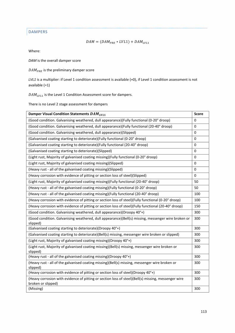
113

DAMPERS

𝐷𝐴𝑀 = (𝐷𝐴𝑀𝑃𝑅𝐸 ∗ 𝐿𝑉𝐿1) + 𝐷𝐴𝑀𝐿𝑉𝐿1

Where:

DAM is the overall damper score

𝐷𝐴𝑀𝑃𝑅𝐸 is the preliminary damper score


available (=1)

𝐷𝐴𝑀𝐿𝑉𝐿1 is the Level 1 Condition Assessment score for dampers.

There is no Level 2 stage assessment for dampers

Damper Visual Condition Statements 𝑫𝑨𝑴𝑳𝑽𝑳𝟏 Score

(Good condition. Galvanising weathered, dull appearance)(Fully functional (0-20° droop) 0

(Good condition. Galvanising weathered, dull appearance)(Fully functional (20-40° droop) 0

(Good condition. Galvanising weathered, dull appearance)(Slipped) 0

(Galvanised coating starting to deteriorate)(Fully functional (0-20° droop) 0

(Galvanised coating starting to deteriorate)(Fully functional (20-40° droop) 0

(Galvanised coating starting to deteriorate)(Slipped) 0

(Light rust, Majority of galvanised coating missing)(Fully functional (0-20° droop) 0

(Light rust, Majority of galvanised coating missing)(Slipped) 0

(Heavy rust - all of the galvanised coating missing)(Slipped) 0

(Heavy corrosion with evidence of pitting or section loss of steel)(Slipped) 0

(Light rust, Majority of galvanised coating missing)(Fully functional (20-40° droop) 50

(Heavy rust - all of the galvanised coating missing)(Fully functional (0-20° droop) 50

(Heavy rust - all of the galvanised coating missing)(Fully functional (20-40° droop) 100

(Heavy corrosion with evidence of pitting or section loss of steel)(Fully functional (0-20° droop) 100

(Heavy corrosion with evidence of pitting or section loss of steel)(Fully functional (20-40° droop) 150

(Good condition. Galvanising weathered, dull appearance)(Droopy 40°+) 300

(Good condition. Galvanising weathered, dull appearance)(Bell(s) missing, messenger wire broken or slipped)

300

(Galvanised coating starting to deteriorate)(Droopy 40°+) 300

(Galvanised coating starting to deteriorate)(Bell(s) missing, messenger wire broken or slipped) 300

(Light rust, Majority of galvanised coating missing)(Droopy 40°+) 300

(Light rust, Majority of galvanised coating missing)(Bell(s) missing, messenger wire broken or slipped)

300

(Heavy rust - all of the galvanised coating missing)(Droopy 40°+) 300

(Heavy rust - all of the galvanised coating missing)(Bell(s) missing, messenger wire broken or slipped)

300

(Heavy corrosion with evidence of pitting or section loss of steel)(Droopy 40°+) 300

(Heavy corrosion with evidence of pitting or section loss of steel)(Bell(s) missing, messenger wire broken or slipped)

300

(Missing) 300

114

INSULATORS

𝐼𝑁𝑆 = (𝐼𝑁𝑆𝑃𝑅𝐸 ∗ 𝐿𝑉𝐿1) + (𝐼𝑁𝑆𝐹𝐴𝑀 ∗ 𝐿𝑉𝐿2) + (max (𝐼𝑁𝑆𝐿𝑉𝐿1, 𝐼𝑁𝑆𝐿𝑉𝐿2))

Where:

INS is the overall insulator score

𝐼𝑁𝑆𝑃𝑅𝐸 is the preliminary insulator score


available (=1)

𝐼𝑁𝑆𝐹𝐴𝑀 is the Insulator Family Score

𝐿𝑉𝐿2 is a multiplier: if Level 2 condition assessment is available (=0), if Level 2 condition assessment is not

available (=1)

𝐼𝑁𝑆𝐿𝑉𝐿1 is the Level 1 Condition Assessment score for insulators.

𝐼𝑁𝑆𝐿𝑉𝐿2 is the Level 2 Condition Assessment score for insulators.

Insulator Family 𝑰𝑵𝑺𝑭𝑨𝑴 Score

Porcelain 0

Grey Porcelain without zinc collars 100

Brown Porcelain without zinc collars 200

Glass 0

Polymeric 0

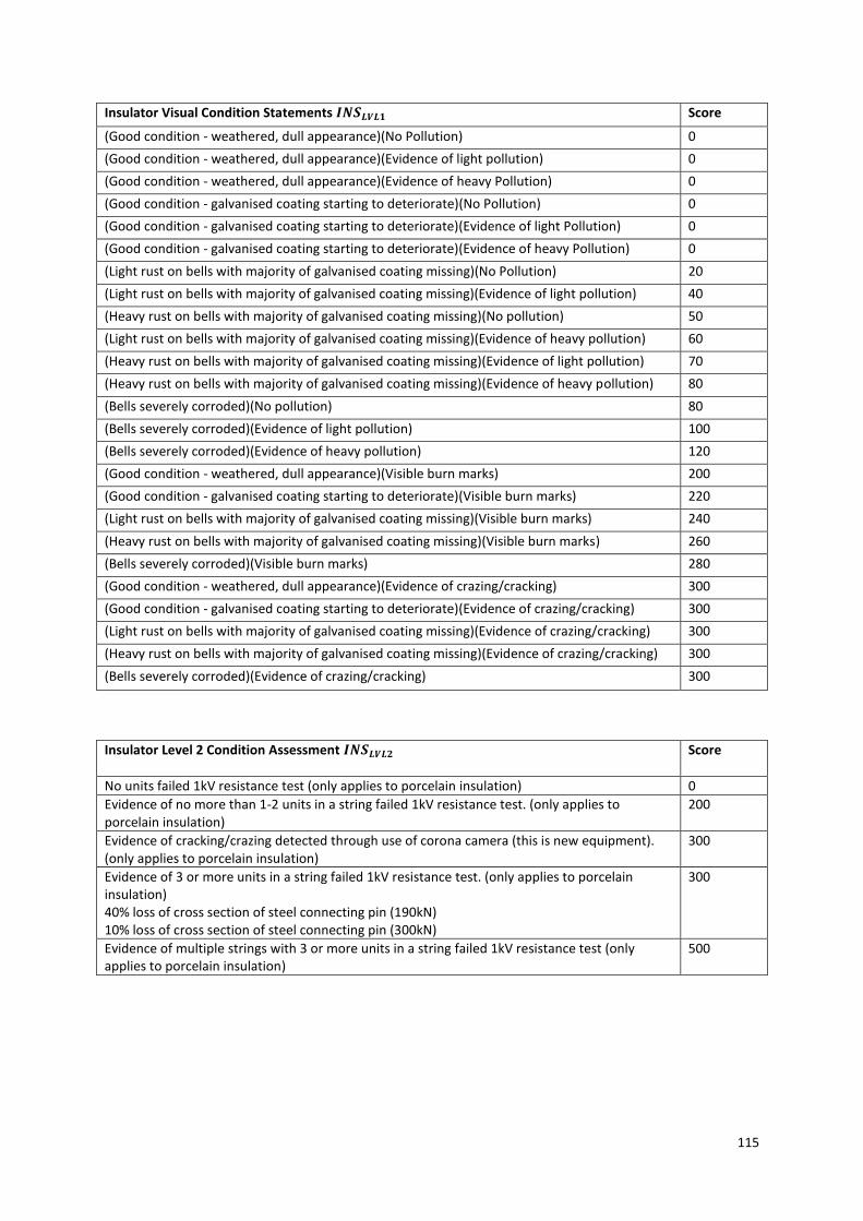
115

Insulator Visual Condition Statements 𝑰𝑵𝑺𝑳𝑽𝑳𝟏 Score

(Good condition - weathered, dull appearance)(No Pollution) 0

(Good condition - weathered, dull appearance)(Evidence of light pollution) 0

(Good condition - weathered, dull appearance)(Evidence of heavy Pollution) 0

(Good condition - galvanised coating starting to deteriorate)(No Pollution) 0

(Good condition - galvanised coating starting to deteriorate)(Evidence of light Pollution) 0

(Good condition - galvanised coating starting to deteriorate)(Evidence of heavy Pollution) 0

(Light rust on bells with majority of galvanised coating missing)(No Pollution) 20

(Light rust on bells with majority of galvanised coating missing)(Evidence of light pollution) 40

(Heavy rust on bells with majority of galvanised coating missing)(No pollution) 50

(Light rust on bells with majority of galvanised coating missing)(Evidence of heavy pollution) 60

(Heavy rust on bells with majority of galvanised coating missing)(Evidence of light pollution) 70

(Heavy rust on bells with majority of galvanised coating missing)(Evidence of heavy pollution) 80

(Bells severely corroded)(No pollution) 80

(Bells severely corroded)(Evidence of light pollution) 100

(Bells severely corroded)(Evidence of heavy pollution) 120

(Good condition - weathered, dull appearance)(Visible burn marks) 200

(Good condition - galvanised coating starting to deteriorate)(Visible burn marks) 220

(Light rust on bells with majority of galvanised coating missing)(Visible burn marks) 240

(Heavy rust on bells with majority of galvanised coating missing)(Visible burn marks) 260

(Bells severely corroded)(Visible burn marks) 280

(Good condition - weathered, dull appearance)(Evidence of crazing/cracking) 300

(Good condition - galvanised coating starting to deteriorate)(Evidence of crazing/cracking) 300

(Light rust on bells with majority of galvanised coating missing)(Evidence of crazing/cracking) 300

(Heavy rust on bells with majority of galvanised coating missing)(Evidence of crazing/cracking) 300

(Bells severely corroded)(Evidence of crazing/cracking) 300

Insulator Level 2 Condition Assessment 𝑰𝑵𝑺𝑳𝑽𝑳𝟐

Score

No units failed 1kV resistance test (only applies to porcelain insulation) 0

Evidence of no more than 1-2 units in a string failed 1kV resistance test. (only applies to porcelain insulation)

200

Evidence of cracking/crazing detected through use of corona camera (this is new equipment). (only applies to porcelain insulation)

300

Evidence of 3 or more units in a string failed 1kV resistance test. (only applies to porcelain insulation) 40% loss of cross section of steel connecting pin (190kN) 10% loss of cross section of steel connecting pin (300kN)

300

Evidence of multiple strings with 3 or more units in a string failed 1kV resistance test (only applies to porcelain insulation)

500

116

PHASE FITTINGS

𝑃𝐻𝐹 = (𝑃𝐻𝐹𝑃𝑅𝐸 ∗ 𝐿𝑉𝐿1) + 𝑃𝐻𝐹𝐿𝑉𝐿1

Where:

PHF is the overall phase fittings score

𝑃𝐻𝐹𝑃𝑅𝐸 is the preliminary phase fittings score


available (=1)

𝑃𝐻𝐹𝐿𝑉𝐿1 is the Level 1 Condition Assessment score for phase fittings.

Phase Fittings are made up of

1. Suspension Linkages: Shackle, Ball Ended Eye Link, Yoke Plate, Shoes, Maintenance Bracket, Weights,

Straps. (𝐿𝑁𝐾𝑆𝑈𝑆)

2. Tension Linkages: Landing Pin, Shackle, Ball Ended Eye Link, Straps, Yoke Plate. (𝐿𝑁𝐾𝑇𝐸𝑁)

3. Arcing Horns and Corona Rings. (ARC)

4. Dowel Pins and Bolts. (DOW)

𝑃𝐻𝐹𝐿𝑉𝐿1 = max ((𝑚𝑎𝑥(𝐿𝑁𝐾𝑆𝑈𝑆)), (𝑚𝑎𝑥(𝐿𝑁𝐾𝑇𝐸𝑁)), 𝐴𝑅𝐶, 𝐷𝑂𝑊)

The max(LNKSUS) means maximum of all suspicion leakages in the route. Max(LNKTEN) means maximum of all

tension linkages in the route.

These have their own set of condition statements and scores as set out below.

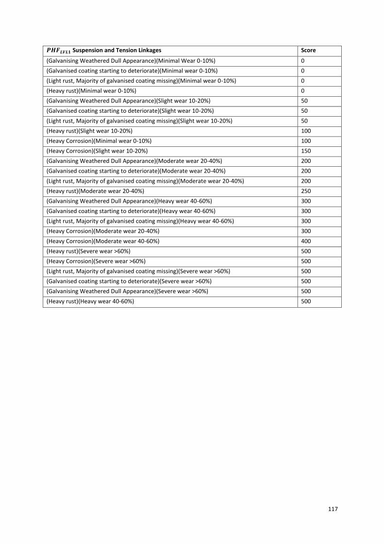
117

𝑷𝑯𝑭𝑳𝑽𝑳𝟏 Suspension and Tension Linkages Score

(Galvanising Weathered Dull Appearance)(Minimal Wear 0-10%) 0

(Galvanised coating starting to deteriorate)(Minimal wear 0-10%) 0

(Light rust, Majority of galvanised coating missing)(Minimal wear 0-10%) 0

(Heavy rust)(Minimal wear 0-10%) 0

(Galvanising Weathered Dull Appearance)(Slight wear 10-20%) 50

(Galvanised coating starting to deteriorate)(Slight wear 10-20%) 50

(Light rust, Majority of galvanised coating missing)(Slight wear 10-20%) 50

(Heavy rust)(Slight wear 10-20%) 100

(Heavy Corrosion)(Minimal wear 0-10%) 100

(Heavy Corrosion)(Slight wear 10-20%) 150

(Galvanising Weathered Dull Appearance)(Moderate wear 20-40%) 200

(Galvanised coating starting to deteriorate)(Moderate wear 20-40%) 200

(Light rust, Majority of galvanised coating missing)(Moderate wear 20-40%) 200

(Heavy rust)(Moderate wear 20-40%) 250

(Galvanising Weathered Dull Appearance)(Heavy wear 40-60%) 300

(Galvanised coating starting to deteriorate)(Heavy wear 40-60%) 300

(Light rust, Majority of galvanised coating missing)(Heavy wear 40-60%) 300

(Heavy Corrosion)(Moderate wear 20-40%) 300

(Heavy Corrosion)(Moderate wear 40-60%) 400

(Heavy rust)(Severe wear >60%) 500

(Heavy Corrosion)(Severe wear >60%) 500

(Light rust, Majority of galvanised coating missing)(Severe wear >60%) 500

(Galvanised coating starting to deteriorate)(Severe wear >60%) 500

(Galvanising Weathered Dull Appearance)(Severe wear >60%) 500

(Heavy rust)(Heavy wear 40-60%) 500

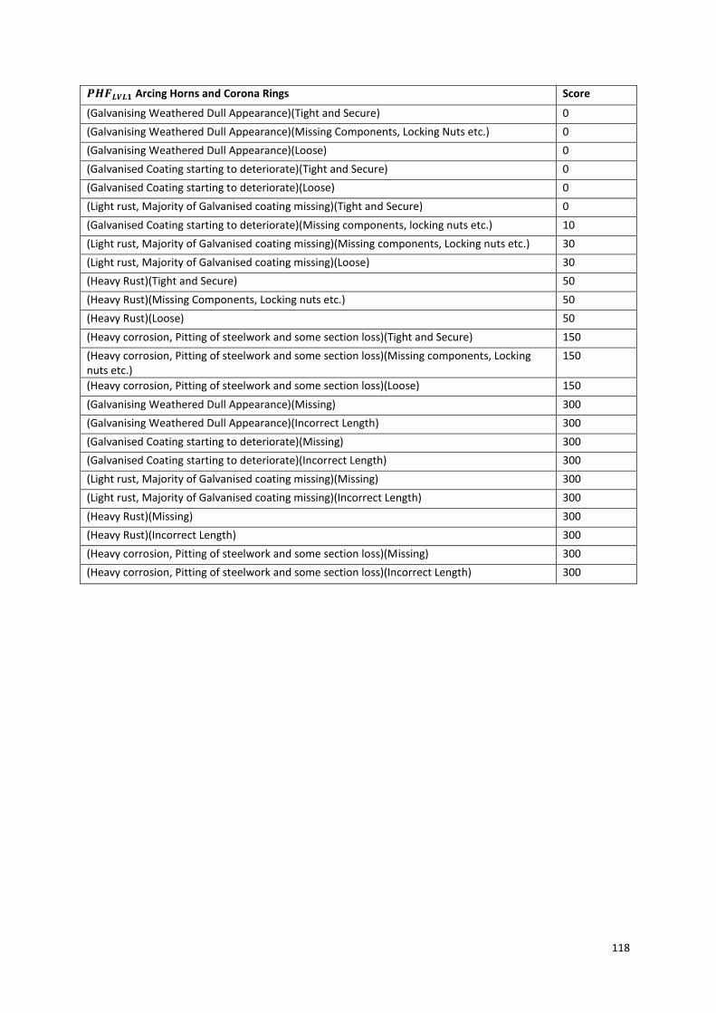
118

𝑷𝑯𝑭𝑳𝑽𝑳𝟏 Arcing Horns and Corona Rings Score

(Galvanising Weathered Dull Appearance)(Tight and Secure) 0

(Galvanising Weathered Dull Appearance)(Missing Components, Locking Nuts etc.) 0

(Galvanising Weathered Dull Appearance)(Loose) 0

(Galvanised Coating starting to deteriorate)(Tight and Secure) 0

(Galvanised Coating starting to deteriorate)(Loose) 0

(Light rust, Majority of Galvanised coating missing)(Tight and Secure) 0

(Galvanised Coating starting to deteriorate)(Missing components, locking nuts etc.) 10

(Light rust, Majority of Galvanised coating missing)(Missing components, Locking nuts etc.) 30

(Light rust, Majority of Galvanised coating missing)(Loose) 30

(Heavy Rust)(Tight and Secure) 50

(Heavy Rust)(Missing Components, Locking nuts etc.) 50

(Heavy Rust)(Loose) 50

(Heavy corrosion, Pitting of steelwork and some section loss)(Tight and Secure) 150

(Heavy corrosion, Pitting of steelwork and some section loss)(Missing components, Locking nuts etc.)

150

(Heavy corrosion, Pitting of steelwork and some section loss)(Loose) 150

(Galvanising Weathered Dull Appearance)(Missing) 300

(Galvanising Weathered Dull Appearance)(Incorrect Length) 300

(Galvanised Coating starting to deteriorate)(Missing) 300

(Galvanised Coating starting to deteriorate)(Incorrect Length) 300

(Light rust, Majority of Galvanised coating missing)(Missing) 300

(Light rust, Majority of Galvanised coating missing)(Incorrect Length) 300

(Heavy Rust)(Missing) 300

(Heavy Rust)(Incorrect Length) 300

(Heavy corrosion, Pitting of steelwork and some section loss)(Missing) 300

(Heavy corrosion, Pitting of steelwork and some section loss)(Incorrect Length) 300

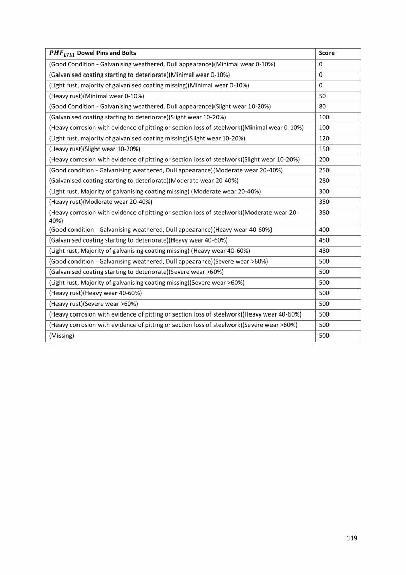
119

𝑷𝑯𝑭𝑳𝑽𝑳𝟏 Dowel Pins and Bolts Score

(Good Condition - Galvanising weathered, Dull appearance)(Minimal wear 0-10%) 0

(Galvanised coating starting to deteriorate)(Minimal wear 0-10%) 0

(Light rust, majority of galvanised coating missing)(Minimal wear 0-10%) 0

(Heavy rust)(Minimal wear 0-10%) 50

(Good Condition - Galvanising weathered, Dull appearance)(Slight wear 10-20%) 80

(Galvanised coating starting to deteriorate)(Slight wear 10-20%) 100

(Heavy corrosion with evidence of pitting or section loss of steelwork)(Minimal wear 0-10%) 100

(Light rust, majority of galvanised coating missing)(Slight wear 10-20%) 120

(Heavy rust)(Slight wear 10-20%) 150

(Heavy corrosion with evidence of pitting or section loss of steelwork)(Slight wear 10-20%) 200

(Good condition - Galvanising weathered, Dull appearance)(Moderate wear 20-40%) 250

(Galvanised coating starting to deteriorate)(Moderate wear 20-40%) 280

(Light rust, Majority of galvanising coating missing) (Moderate wear 20-40%) 300

(Heavy rust)(Moderate wear 20-40%) 350

(Heavy corrosion with evidence of pitting or section loss of steelwork)(Moderate wear 20-40%)

380

(Good condition - Galvanising weathered, Dull appearance)(Heavy wear 40-60%) 400

(Galvanised coating starting to deteriorate)(Heavy wear 40-60%) 450

(Light rust, Majority of galvanising coating missing) (Heavy wear 40-60%) 480

(Good condition - Galvanising weathered, Dull appearance)(Severe wear >60%) 500

(Galvanised coating starting to deteriorate)(Severe wear >60%) 500

(Light rust, Majority of galvanising coating missing)(Severe wear >60%) 500

(Heavy rust)(Heavy wear 40-60%) 500

(Heavy rust)(Severe wear >60%) 500

(Heavy corrosion with evidence of pitting or section loss of steelwork)(Heavy wear 40-60%) 500

(Heavy corrosion with evidence of pitting or section loss of steelwork)(Severe wear >60%) 500

(Missing) 500

120

ENVIRONMENT

𝐸𝑁𝑉 = 𝐸𝑁𝑉𝑊𝐼𝑀 + 𝐸𝑁𝑉𝑃𝑂𝐿

Assessment of the Environment Type is based on the following criteria:

Environment Criteria Score

𝐸𝑁𝑉𝑊𝐼𝑀 Wind Induced Motion – Does Galloping Occur? 30

𝐸𝑁𝑉𝑊𝐼𝑀 Wind Induced Motion – Does Sub conductor Oscillation Occur? 30

𝐸𝑁𝑉𝑊𝐼𝑀 Wind Induced Motion – Significant % of route 150m above sea level? 30

𝐸𝑁𝑉𝑃𝑂𝐿 Pollution – Parts of route within 5 km of the coast? 30

𝐸𝑁𝑉𝑃𝑂𝐿 Pollution – Parts of route within 10km of coast (if answered ‘yes’ to above question (5km) score again in this category)?

30

𝐸𝑁𝑉𝑃𝑂𝐿 Pollution – Heavy Industrial Environment? 30

OVERALL END OF LIFE MODIFIER FOR OHL FITTINGS

The end of life modifier formula for fittings given at the beginning of this section is reproduced below with a

mathematic summary of how each component is determined.

𝑬𝑶𝑳𝒎𝒐𝒅 = 𝐦𝐚𝐱(𝑺𝑷𝑨,𝑫𝑨𝑴, 𝑰𝑵𝑺, 𝑷𝑯𝑭) + 𝑬𝑵𝑽𝑾𝑰𝑴 + 𝑬𝑵𝑽𝑷𝑶𝑳

Where:

𝑆𝑃𝐴 = (𝑆𝑃𝐴𝑃𝑅𝐸 ∗ 𝐿𝑉𝐿1) + 𝑆𝑃𝐴𝐹𝐴𝑀 + 𝑆𝑃𝐴𝐿𝑉𝐿1

𝐷𝐴𝑀 = (𝐷𝐴𝑀𝑃𝑅𝐸 ∗ 𝐿𝑉𝐿1) + 𝐷𝐴𝑀𝐿𝑉𝐿1

𝐼𝑁𝑆 = (𝐼𝑁𝑆𝑃𝑅𝐸 ∗ 𝐿𝑉𝐿1) + (𝐼𝑁𝑆𝐹𝐴𝑀 ∗ 𝐿𝑉𝐿2) + (max (𝐼𝑁𝑆𝐿𝑉𝐿1, 𝐼𝑁𝑆𝐿𝑉𝐿2))

𝑃𝐻𝐹 = (𝑃𝐻𝐹𝑃𝑅𝐸 ∗ 𝐿𝑉𝐿1) + 𝑃𝐻𝐹𝐿𝑉𝐿1

𝑃𝐻𝐹𝐿𝑉𝐿1 = max ((𝑚𝑎𝑥(𝐿𝑁𝐾𝑆𝑈𝑆)), (𝑚𝑎𝑥(𝐿𝑁𝐾𝑇𝐸𝑁)), 𝐴𝑅𝐶, 𝐷𝑂𝑊)

121

APPENDIX III – SP TRANSMISSION / SHE-TRANSMISSION

This Appendix provides supplemental information where required as well as further detail on how SP

Transmission and SHE Transmission implement the methodology laid out within the main document. For ease

of navigation, it follows as far as possible the same layout as Sections 5 and 6 of the Methodology. Where a

part of these sections is not referred to below, it is to be assumed that there is no deviation from, or further

information to be added to, the Common Methodology.

1. METHODOLOGY OVERVIEW

A. ASSET

In order to ascertain the overall level of risk, the methodology will calculate Asset Risk for lead assets only,

namely:

Circuit Breakers

Transformers

Reactors

Underground Cable

Overhead Lines

o Conductor

o Fittings

o Towers

Whilst we have a small 33kV asset base, lead assets are deemed by Ofgem to be those operating at 132kV and

above.

B. MATERIAL FAILURE MODE

The failure criteria for each asset is a state that prevents the achievement specified requirement and function.

By implication, any state that does not prevent or impede the achievement of the specified requirement and

function is not regarded as a failure. The SP Transmission/SHE Transmission implementation of this

methodology (referred to hereafter as “the Implementation”) considers only the condition-related failure

modes with measurable effects on the specified requirement and function.

The Implementation allows for up to five condition-related failure modes and each failure mode is defined

according the severity of the consequences. In order to adequately assess the effect or criticality of each

failure mode (in accordance with Section 5.2.9 of EN 60812), these definitions are specific to each asset class

and are defined in the relevant section

C. PROBABILITY OF DETECTION

The probability of detecting and acting upon the failure mode is already covered in the definition of the failure

modes and the use of actual data on the number of failures to calibrate the model (i.e. if a failure mode if

usually detected early then this will reflected in the fact that more of the failures will be in the category

addressed by planned outages.

D. PROBABILITY OF CONSEQUENCE

As stated in the common methodology, this function is used when a failure mode is mapped to multiple

effects. However, as this deployment of the methodology considers only the condition-related failure modes

122

with measurable effects on the specified requirement and function, there is a one-to-one mapping from failure

mode to effect and, therefore, this is not required.

2. FMEA

As stated within BS 60812, “The lowest level within the system at which the analysis is effective is that level for

which information is available… Less detailed analysis may be justified for a system based on a mature design,

with a good reliability, maintainability and safety record”. This deployment of FMEA is a flexible and practical

implementation of theory which has been shown to align with BS 60812.

It is not a top down approach, but a system level approach (e.g., transformer) rather than a sub-component

level approach (e.g., tapchanger selector). The advantage of this approach is that the same failure mode

effects are still considered without the level of uncertainty required for sub-component level analysis.

This system level approach looks at failure modes and their effects, whilst the subcomponent level approach

looks at the causes of these failure modes. This subcomponent level approach necessitates a degree of

assumption as it requires the operator to define the most likely failure modes (and effects) for each failure

cause.

1. UNDERSTANDING FAILURE CAUSE TYPES ON TO ASSETS

BS 60812 states:

“The identification and description of failure causes is not always necessary for all failure modes identified in

the analysis. Identification and description of failure causes, as well as suggestions for their mitigation should

be done on the basis of the failure effects and their severity. The more severe the effects of failure modes, the

more accurately failure causes should be identified and described. Otherwise, the analyst may dedicate

unnecessary effort on the identification of failure causes of such failure modes that have no or a very minor

effect on system functionality.”

In line with the Standard, this methodology does not require the documentation of all failure causes for each

failure mode. As electrical assets are based on mature designs with many years of experience of the assets in

service, the failure causes are well researched and understood, with many years worth of publications, failure

investigations and in-service experience of most designs. As such, mitigations for these failure causes are also

relatively mature and have resulted in proven design changes, or the ability to detect these failure causes

before they lead to catastrophic failure of the asset. This methodology takes this ability to detect the failure

causes into consideration when defining the data used to calculate the probability of failure. By providing a

flexible framework for the probability of failure calculation, the methodology can take account of any variation

in failure causes and detection methods between different asset designs.

Although the potential failure causes could be identified and documented for every failure mode for every

asset type, this is considered to be unnecessary effort for a mature and well understood asset base. In

addition, a significant number of the failure causes will be exhibited in the same way and have the same

severity of their effect e.g. a gassing transformer may be caused by a high resistance connection, movement of

the winding, failure of the insulation etc., but all have the potential to result the same failure effect e.g. a

Buchholz trip which requires further investigation. Only after investigation will the actual cause of the failure

be evident, so the use of field data to define the failure rates for the each of the failure effects and related

failure modes is considered to give a more reliable output:

123

“Failure causes may be determined from analysis of field failures or failures in test units. When the design is

new and without precedent, failure causes may be established by eliciting the opinion of experts.”

A. FAILURE MODES

This methodology includes the ability to model up to 5 condition failure modes. The failure modes are grouped

in the same way as the common methodology, with the failure modes may be defined as:

Defect: A failure that can be repaired with a planned outage and returned to service within 24 hours.

Minor failure: A failure that causes an unplanned outage which can be repaired and returned to

service within 24 hours.

Significant failure: A failure that causes an unplanned outage which can be repaired; the duration of

the repair exceeds 24 hours but is less than 10 days.

Major failure: A failure that causes an unplanned outage which causes extensive damage. Where

repairs are possible, the duration exceeds 10 days. Alternatively, the failure requires the installation

of a new asset.

The failure modes will also be inherently considered at the level below these groupings so that consideration

of the severity (consequence) of failure, and failure rates can be aligned to actual failure data. Examples for a

transformer are shown below:

Defect e.g. External damage to transformer

Minor Failure e.g. Buchholz trip – no evident fault

Significant Failure

e.g. Bushing or tapchanger failure requiring replacement of component

Major Failure e.g. Winding failure requiring replacement of asset

The failure modes considered in this methodology, along with their effects and failure rates, are designed to

be completely flexible so that they can be aligned with the actual failure modes experienced for an asset group

and aligned with actual failure data. For example, failure modes used in transmission may be calibrated

differently to those used for distribution assets in cases where inherently different management strategies are

applied.

B. DETECTING FAILURE MODES

The standard states that “For each failure mode, the analyst should determine the way in which the failure is

detected and the means by which the user or maintainer is made aware of the failure.”

As the failure modes are defined at system level in this methodology and directly linked to the failure effects,

the some of the failure modes will be detected if an outage occurs, others will be detected during inspection,

maintenance or testing of the asset, and these detection methods will generally be aligned with the data

included in determination of the asset health within CBRM. As such the End of Life and Probability of Failure

can be directly linked through the inclusion of the appropriate measurement data.

C. CONSEQUENCE OF FAILURE MODES

As stated above, only the failure modes with measurable effects on the specified requirement and function are

considered. The failure modes are summarised according to the severity of the failure effect.

124

A typical summary of consequences is provided below:

Defect: A failure which could have the potential to cause a significant or major failure in the future. A

short outage may be required to remediate the defect.

Minor failure: A failure that causes an unplanned outage which can be repaired and returned to service

within 24 hours.

Significant failure: A failure that causes an unplanned outage which can be repaired; the duration of the

repair exceeds 24 hours but is less than 10 days.

Major failure: A failure that causes an unplanned outage which causes extensive damage. Where

repairs are possible, the duration exceeds 10 days. Alternatively, the failure requires the installation of

a new asset.

This technique of summarising consequences according to the severity of each failure mode has two

advantages:

1) Only those failure modes with material effects are included, avoiding any unnecessary analysis of

failure modes that do not have material effects, and;

2) Direct alignment with the failure severity classification, thereby reducing any uncertainty in the

mapping of failure effect to failure severity.

This approach has been found to give accurate, reproducible results using generally available data and as a

result has been widely adopted throughout the industry both within Great Britain and overseas. For further

information on this approach, please see “Determination of K”.

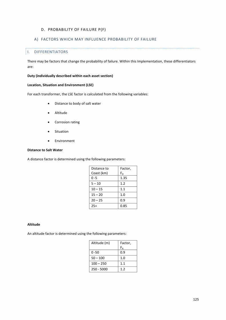
125

D. PROBABILITY OF FAILURE P(F)

A) FACTORS WHICH MAY INFLUENCE PROBABILITY OF FAILURE

I. DIFFERENTIATORS

There may be factors that change the probability of failure. Within this Implementation, these differentiators

are:

Duty (individually described within each asset section)

Location, Situation and Environment (LSE)

For each transformer, the LSE factor is calculated from the following variables:

Distance to body of salt water

Altitude

Corrosion rating

Situation

Environment

Distance to Salt Water

A distance factor is determined using the following parameters:

Distance to Coast (km)

Factor, FD

0 -5 1.35

5 – 10 1.2

10 – 15 1.1

15 – 20 1.0

20 – 25 0.9

25+ 0.85

Altitude

An altitude factor is determined using the following parameters:

Altitude (m) Factor, FA

0 -50 0.9

50 – 100 1.0

100 – 250 1.1

250 - 5000 1.2

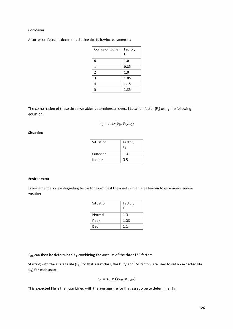
126

Corrosion

A corrosion factor is determined using the following parameters:

Corrosion Zone Factor, FC

0 1.0

1 0.85

2 1.0

3 1.05

4 1.15

5 1.35

The combination of these three variables determines an overall Location factor (FL) using the following

equation:

FL = max(FD, FA, FC)

Situation

Situation Factor, FS

Outdoor 1.0

Indoor 0.5

Environment

Environment also is a degrading factor for example if the asset is in an area known to experience severe

weather.

Situation Factor, FE

Normal 1.0

Poor 1.06

Bad 1.1

FLSE can then be determined by combining the outputs of the three LSE factors.

Starting with the average life (LA) for that asset class, the Duty and LSE factors are used to set an expected life

(LE) for each asset.

𝐿𝐸 = 𝐿𝐴 × (𝐹𝐿𝑆𝐸 × 𝐹𝐷𝑌)

This expected life is then combined with the average life for that asset type to determine HI1.

127

II. MODIFIERS

Modifiers change the rate at which an asset’s Probability of Failure increases. Within this Implementation,

these modifiers are:

Where they differ from the descriptions above, or are asset-type specific, these factors are described in more

detail in the asset specific sections of this Appendix (Sections 6-9 of this chapter).

Visual External Condition Factors

The observed condition of the transformer is evaluated through visual assessment by operational staff.

Several components of the transformer and assessed individually and assigned a condition. Condition is

assessed on a 1-5 scale (1 = satisfactory, 5 = immediate replacement required). Each component’s condition is

weighted differently based on the significance of the component. These components are combined to produce

an overall scale and a Condition factor is produced.

Condition Score Factor, FR

1 0.75

2 1.0

3 1.1

4 1.25

5 1.5

Defects

The defect module searches the input data defect list to identify any defects associated with each asset. The

defects, in the form of stock phrases, automatically populate a defects calibration table against which users

assign a defect severity score. Once the calibration table has been set, the defect module calculates a defect

score for each asset, and uses this score to determine a defect factor, which can be overridden by a poor

defect history exception report. As with the condition factor outlined above, it is possible to set minimum HIs

for any identified defects, where this has taken place the model will identify any minimum EoL indices, and set

them aside for use later in the process.

Family Reliability

Family Reliability is determined using the TO’s own experience of assets in operation. Each family is assigned a

reliability rating (from 1-4, with 1 being Very Reliable and 4 being Very Unreliable) which then generates a

reliability factor, based on the following parameters:

Reliability Score Factor, FR

1 0.85

2 1.0

3 1.15

4 1.35

128

Oil Condition Test Results (SP Transmission only)

Oil condition test results are used to derive an oil condition test factor. Results include moisture, acidity and

breakdown strength. The results (either pass, suspect or fail) for each test type are used to derive individual

test factors (and if desired minimum EoL indices) and are then combined in order to produce an overall test

factor. The overall test factor is included in the formation of modifying factor FV1, while any defined minimum

EoL indices are set aside for use later in the process.

Test Results

Where tests have been undertaken, the results (either pass, suspect or fail) for each test type are used to

derive individual test factors (and if desired minimum EoL indices) and are then combined in order to produce

an overall test factor. The overall test factor is included in the formation of modifying factor FV1, while any

defined minimum EoL indices are set aside for use later in the process.

Operational Restrictions

When a significant issue is identified regarding a family of transformers, an Operator can issue a NEDER which

notifies all other operators. This is called an Operational Restriction, or OR. Each OR is assigned a severity,

which then generates an Operational Restriction factor based on the following parameters:

OR Severity Description (example)

Factor, FOR

1 No Effect on Condition

0.85

2 Pre-Operation Checks

1.0

3 Do Not Operate Live

1.15

4 Exclusion Zone 1.35

For assets which have more than one OR assigned to them, it is the largest factor (or most serious OR) which is

passed through to form the overall OR factor.

After-Fault Maintenance (SHE Transmission only)

For assets which have after fault maintenance (AFM), scores, (i.e. assets whose arc extinguishing medium is

either vacuum or SF6), the AFM Score module considers the rate of change of each assets AFM score to

estimate an “extrapolated life”. This estimation is used to determine an AFM factor which is used within the

“FV1” derivation. SP Transmission does not undertake after fault maintenance scoring, and therefore this

parameter is not applicable to SP Transmission circuit breakers.

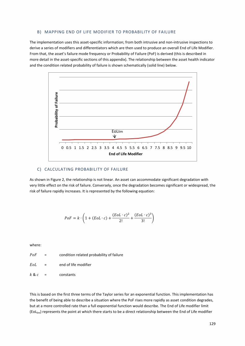
129

B) MAPPING END OF LIFE MODIFIER TO PROBABILITY OF FAILURE

The implementation uses this asset-specific information; from both intrusive and non-intrusive inspections to

derive a series of modifiers and differentiators which are then used to produce an overall End of Life Modifier.

From that, the asset’s failure mode frequency or Probability of Failure (PoF) is derived (this is described in

more detail in the asset-specific sections of this appendix). The relationship between the asset health indicator

and the condition related probability of failure is shown schematically (solid line) below.

C) CALCULATING PROBABILITY OF FAILURE

As shown in Figure 2, the relationship is not linear. An asset can accommodate significant degradation with

very little effect on the risk of failure. Conversely, once the degradation becomes significant or widespread, the

risk of failure rapidly increases. It is represented by the following equation:

𝑃𝑜𝐹 = 𝑘 ∙ (1 + (𝐸𝑜𝐿 ∙ 𝑐) +(𝐸𝑜𝐿 ∙ 𝑐)2

2!+(𝐸𝑜𝐿 ∙ 𝑐)3

3!)

where:

𝑃𝑜𝐹 = condition related probability of failure

𝐸𝑜𝐿 = end of life modifier

𝑘 & 𝑐 = constants

This is based on the first three terms of the Taylor series for an exponential function. This implementation has

the benefit of being able to describe a situation where the PoF rises more rapidly as asset condition degrades,

but at a more controlled rate than a full exponential function would describe. The End of Life modifier limit

(EoLlim) represents the point at which there starts to be a direct relationship between the End of Life modifier

0 0.5 1 1.5 2 2.5 3 3.5 4 4.5 5 5.5 6 6.5 7 7.5 8 8.5 9 9.5 10

Pro

bab

ility

of

Failu

re

End of Life Modifier

EoLlim

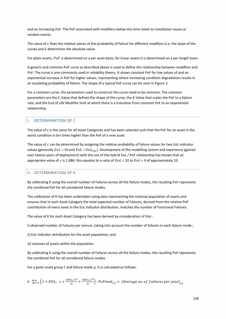
130

and an increasing PoF. The PoF associated with modifiers below this limit relate to installation issues or

random events.

The value of 𝑐 fixes the relative values of the probability of failure for different modifiers (i.e. the slope of the

curve) and 𝑘 determines the absolute value.

For plant assets, 𝑃𝑜𝐹 is determined on a per asset basis; for linear assets it is determined on a per length basis.

A generic and common PoF curve as described above is used to define the relationship between modifiers and

PoF. The curve is one commonly used in reliability theory. It shows constant PoF for low values of and an

exponential increase in PoF for higher values, representing where increasing condition degradation results in

an escalating probability of failure. The shape of a typical PoF curve can be seen in Figure 3.

For a common curve, the parameters used to construct the curve need to be common. The common

parameters are the C-Value that defines the shape of the curve, the K-Value that scales the PoF to a failure

rate, and the End of Life Modifier limit at which there is a transition from constant PoF to an exponential

relationship.

I. DETERMINATION OF C

The value of c is the same for all Asset Categories and has been selected such that the PoF for an asset in the

worst condition is ten times higher than the PoF of a new asset.

The value of 𝑐 can be determined by assigning the relative probability of failure values for two EoL indicator

values (generally 𝐸𝑜𝐿 = 10 and 𝐸𝑜𝐿 = 𝐸𝑜𝐿𝑙𝑖𝑚). Development of the modelling system and experience (gained

over twelve years of deployment) with the use of the hybrid EoL / PoF relationship has shown that an

appropriate value of 𝑐 is 1.086; this equates to a ratio of 𝐸𝑜𝐿 = 10 to 𝐸𝑜𝐿 = 4 of approximately 10.

II. DETERMINATION OF K

By calibrating K using the overall number of Failures across all the failure modes, the resulting PoF represents

the combined PoF for all considered failure modes.

The calibration of K has been undertaken using data representing the national population of assets and

ensures that in each Asset Category the total expected number of Failures, derived from the relative PoF

contribution of every asset in the EoL Indicator distribution, matches the number of Functional Failures.

The value of K for each Asset Category has been derived by consideration of the:-

i) observed number of Failures per annum, taking into account the number of failures in each failure mode ;

ii) EoL Indicator distribution for the asset population; and

iii) volumes of assets within the population.

By calibrating K using the overall number of Failures across all the failure modes, the resulting PoF represents

the combined PoF for all considered failure modes.

For a given asset group 𝐼 and failure mode 𝑞, it is calculated as follows:

𝑘 ∙ ∑ (1 + 𝐸𝑂𝐿𝑖 ∙ 𝑐 +(𝐸𝑂𝐿𝑖∙𝑐)

2

2!+(𝐸𝑂𝐿𝑖∙𝑐)

3

3!)𝑛

𝑖=1 ∙ 𝑃𝑜𝐹𝑚𝑜𝑑𝑖,𝑞 = (𝐴𝑣𝑒𝑟𝑎𝑔𝑒 𝑛𝑜. 𝑜𝑓 𝑓𝑎𝑖𝑙𝑢𝑟𝑒𝑠 𝑝𝑒𝑟 𝑦𝑒𝑎𝑟)𝐼,𝑞

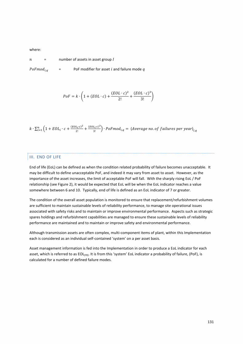
131

where:

𝑛 = number of assets in asset group 𝐼

𝑃𝑜𝐹𝑚𝑜𝑑𝑖,𝑞 = PoF modifier for asset 𝑖 and failure mode 𝑞

𝑃𝑜𝐹 = 𝑘 ∙ (1 + (𝐸𝑂𝐿 ∙ 𝑐) +(𝐸𝑂𝐿 ∙ 𝑐)2

2!+(𝐸𝑂𝐿 ∙ 𝑐)3

3!)

𝑘 ∙ ∑ (1 + 𝐸𝑂𝐿𝑖 ∙ 𝑐 +(𝐸𝑂𝐿𝑖∙𝑐)

2

2!+(𝐸𝑂𝐿𝑖∙𝑐)

3

3!)𝑛

𝑖=1 ∙ 𝑃𝑜𝐹𝑚𝑜𝑑𝑖,𝑞 = (𝐴𝑣𝑒𝑟𝑎𝑔𝑒 𝑛𝑜. 𝑜𝑓 𝑓𝑎𝑖𝑙𝑢𝑟𝑒𝑠 𝑝𝑒𝑟 𝑦𝑒𝑎𝑟)𝐼,𝑞

III. END OF LIFE

End of life (EoL) can be defined as when the condition related probability of failure becomes unacceptable. It

may be difficult to define unacceptable PoF, and indeed it may vary from asset to asset. However, as the

importance of the asset increases, the limit of acceptable PoF will fall. With the sharply rising EoL / PoF

relationship (see Figure 2), it would be expected that EoL will be when the EoL indicator reaches a value

somewhere between 6 and 10. Typically, end of life is defined as an EoL indicator of 7 or greater.

The condition of the overall asset population is monitored to ensure that replacement/refurbishment volumes

are sufficient to maintain sustainable levels of reliability performance, to manage site operational issues

associated with safety risks and to maintain or improve environmental performance. Aspects such as strategic

spares holdings and refurbishment capabilities are managed to ensure these sustainable levels of reliability

performance are maintained and to maintain or improve safety and environmental performance.

Although transmission assets are often complex, multi-component items of plant, within this Implementation

each is considered as an individual self-contained ‘system’ on a per asset basis.

Asset management information is fed into the Implementation in order to produce a EoL indicator for each

asset, which is referred to as EOL(Y0). It is from this ‘system’ EoL indicator a probability of failure, (PoF), is

calculated for a number of defined failure modes.

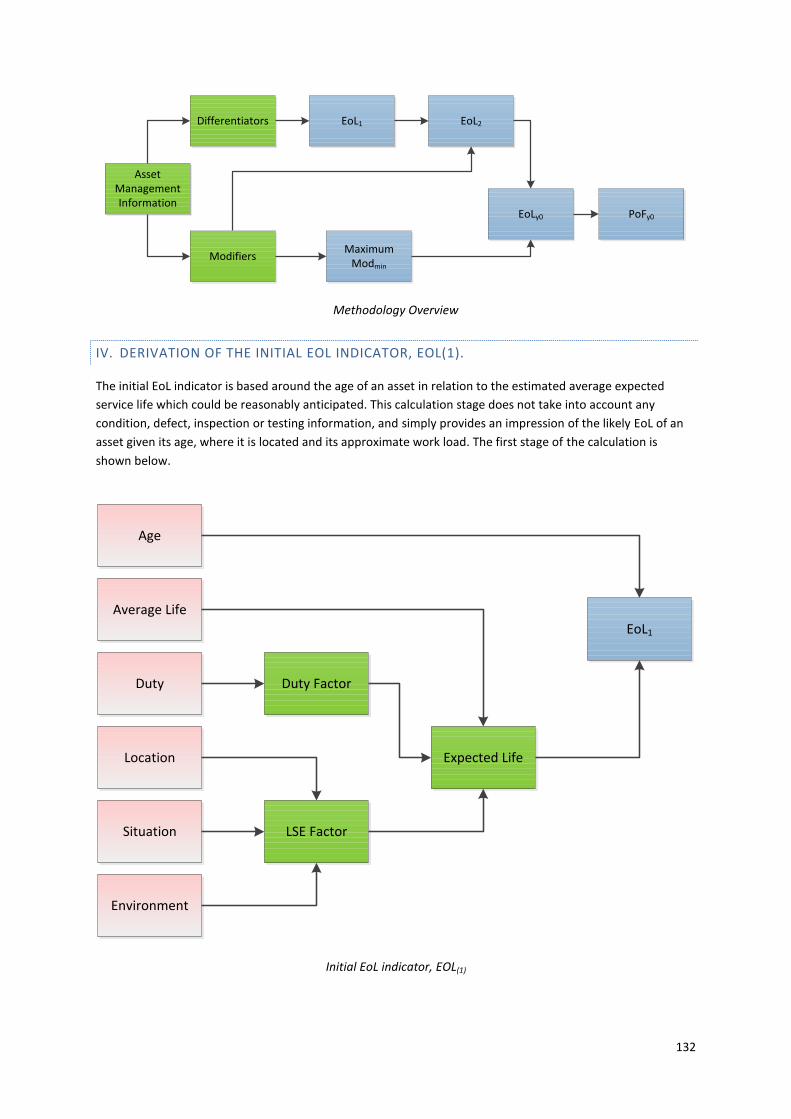
132

Methodology Overview

IV. DERIVATION OF THE INITIAL EOL INDICATOR, EOL(1).

The initial EoL indicator is based around the age of an asset in relation to the estimated average expected

service life which could be reasonably anticipated. This calculation stage does not take into account any

condition, defect, inspection or testing information, and simply provides an impression of the likely EoL of an

asset given its age, where it is located and its approximate work load. The first stage of the calculation is

shown below.

Initial EoL indicator, EOL(1)


EoL1

Maximum Modmin

EoL2

EoLy0

Differentiators

Modifiers

PoFy0

Age

Average Life

Duty

Location

Situation

Environment

LSE Factor

Expected Life

Duty Factor

EoL1

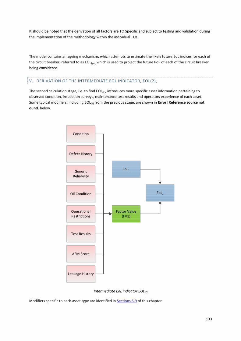
133

It should be noted that the derivation of all factors are TO Specific and subject to testing and validation during

the implementation of the methodology within the individual TOs.

The model contains an ageing mechanism, which attempts to estimate the likely future EoL indices for each of

the circuit breaker, referred to as EOL(yn), which is used to project the future PoF of each of the circuit breaker

being considered.

V. DERIVATION OF THE INTERMEDIATE EOL INDICATOR, EOL(2),

The second calculation stage, i.e. to find EOL(2), introduces more specific asset information pertaining to

observed condition, inspection surveys, maintenance test results and operators experience of each asset.

Some typical modifiers, including EOL(1) from the previous stage, are shown in Error! Reference source not

ound. below.

Intermediate EoL indicator EOL(2)

Modifiers specific to each asset type are identified in Sections 6-9 of this chapter.

Condition

Defect History

Generic Reliability

Oil Condition

Operational Restrictions

Test Results

Factor Value (FV1)

EoL1

AFM Score

Leakage History

EoL2

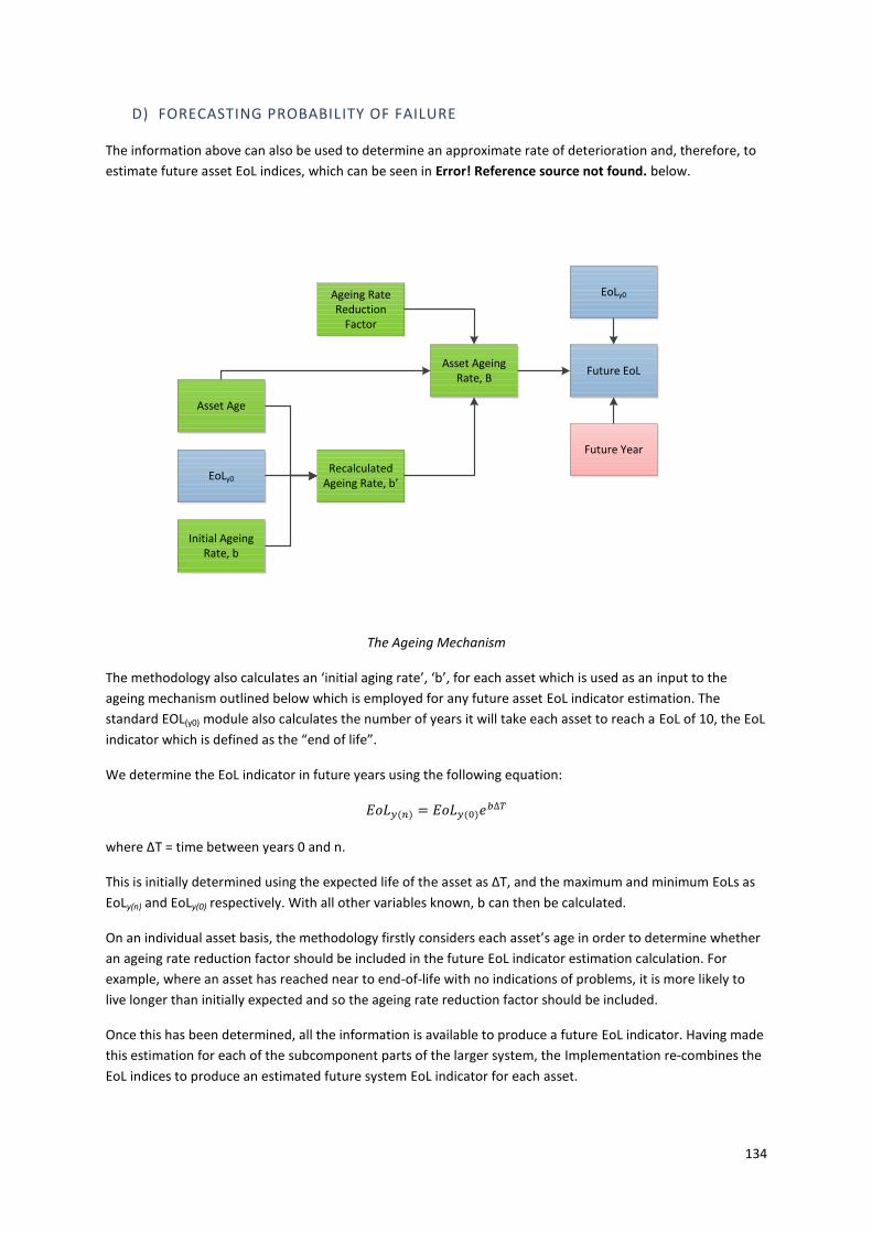
134

D) FORECASTING PROBABILITY OF FAILURE

The information above can also be used to determine an approximate rate of deterioration and, therefore, to

estimate future asset EoL indices, which can be seen in Error! Reference source not found. below.

Asset Age

Initial Ageing Rate, b

EoLy0Recalculated

Ageing Rate, b’

Ageing Rate Reduction

Factor

Asset Ageing Rate, B

Future EoL

Future Year

EoLy0

The Ageing Mechanism

The methodology also calculates an ‘initial aging rate’, ‘b’, for each asset which is used as an input to the

ageing mechanism outlined below which is employed for any future asset EoL indicator estimation. The

standard EOL(y0) module also calculates the number of years it will take each asset to reach a EoL of 10, the EoL

indicator which is defined as the “end of life”.

We determine the EoL indicator in future years using the following equation:

𝐸𝑜𝐿𝑦(𝑛) = 𝐸𝑜𝐿𝑦(0)𝑒𝑏∆𝑇

where ∆T = time between years 0 and n.

This is initially determined using the expected life of the asset as ∆T, and the maximum and minimum EoLs as

EoLy(n) and EoLy(0) respectively. With all other variables known, b can then be calculated.

On an individual asset basis, the methodology firstly considers each asset’s age in order to determine whether

an ageing rate reduction factor should be included in the future EoL indicator estimation calculation. For

example, where an asset has reached near to end-of-life with no indications of problems, it is more likely to

live longer than initially expected and so the ageing rate reduction factor should be included.

Once this has been determined, all the information is available to produce a future EoL indicator. Having made

this estimation for each of the subcomponent parts of the larger system, the Implementation re-combines the

EoL indices to produce an estimated future system EoL indicator for each asset.

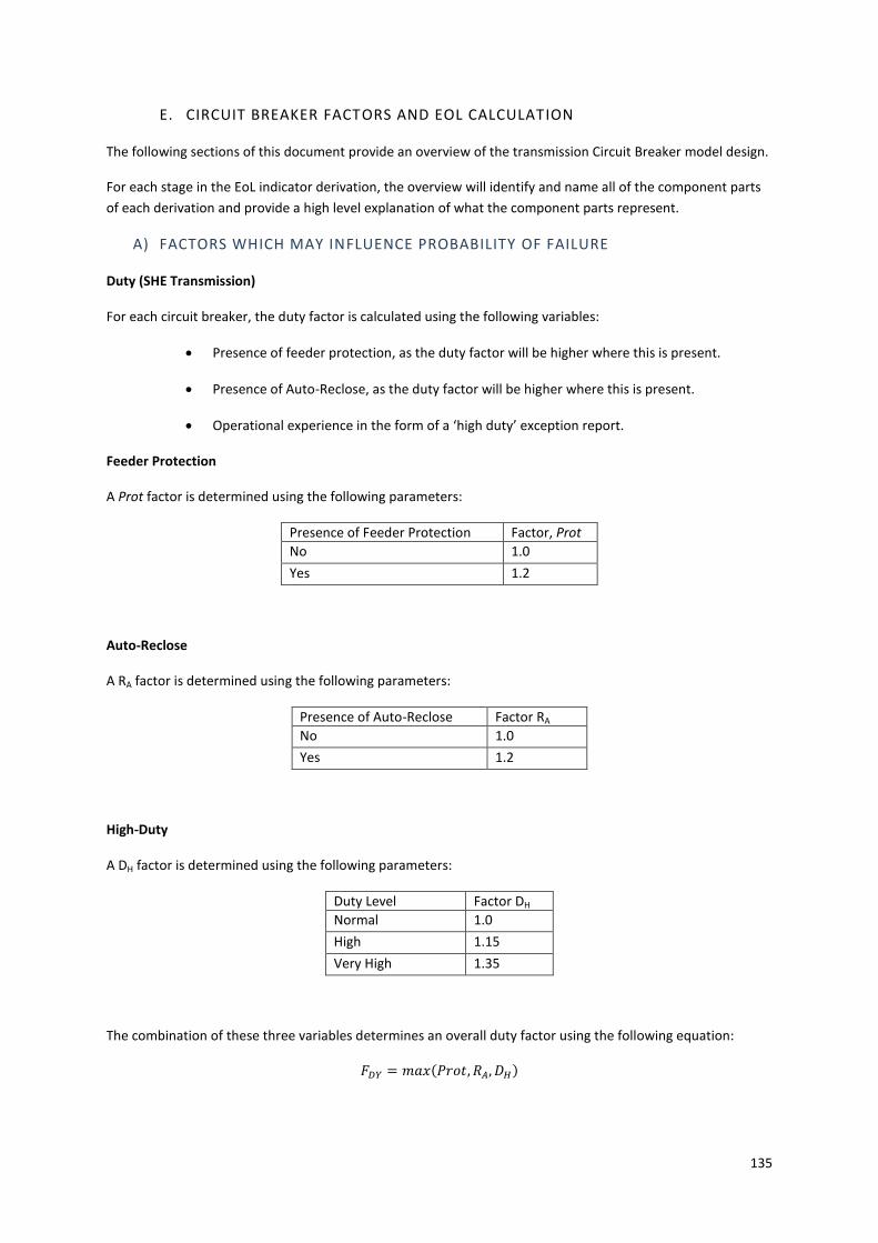
135

E. CIRCUIT BREAKER FACTORS AND EOL CALCULATION

The following sections of this document provide an overview of the transmission Circuit Breaker model design.

For each stage in the EoL indicator derivation, the overview will identify and name all of the component parts

of each derivation and provide a high level explanation of what the component parts represent.


Duty (SHE Transmission)

For each circuit breaker, the duty factor is calculated using the following variables:

Presence of feeder protection, as the duty factor will be higher where this is present.

Presence of Auto-Reclose, as the duty factor will be higher where this is present.

Operational experience in the form of a ‘high duty’ exception report.

Feeder Protection

A Prot factor is determined using the following parameters:

Presence of Feeder Protection Factor, Prot

No 1.0

Yes 1.2

Auto-Reclose

A RA factor is determined using the following parameters:

Presence of Auto-Reclose Factor RA

No 1.0

Yes 1.2

High-Duty

A DH factor is determined using the following parameters:

Duty Level Factor DH

Normal 1.0

High 1.15

Very High 1.35

The combination of these three variables determines an overall duty factor using the following equation:

𝐹𝐷𝑌 = 𝑚𝑎𝑥(𝑃𝑟𝑜𝑡, 𝑅𝐴, 𝐷𝐻)

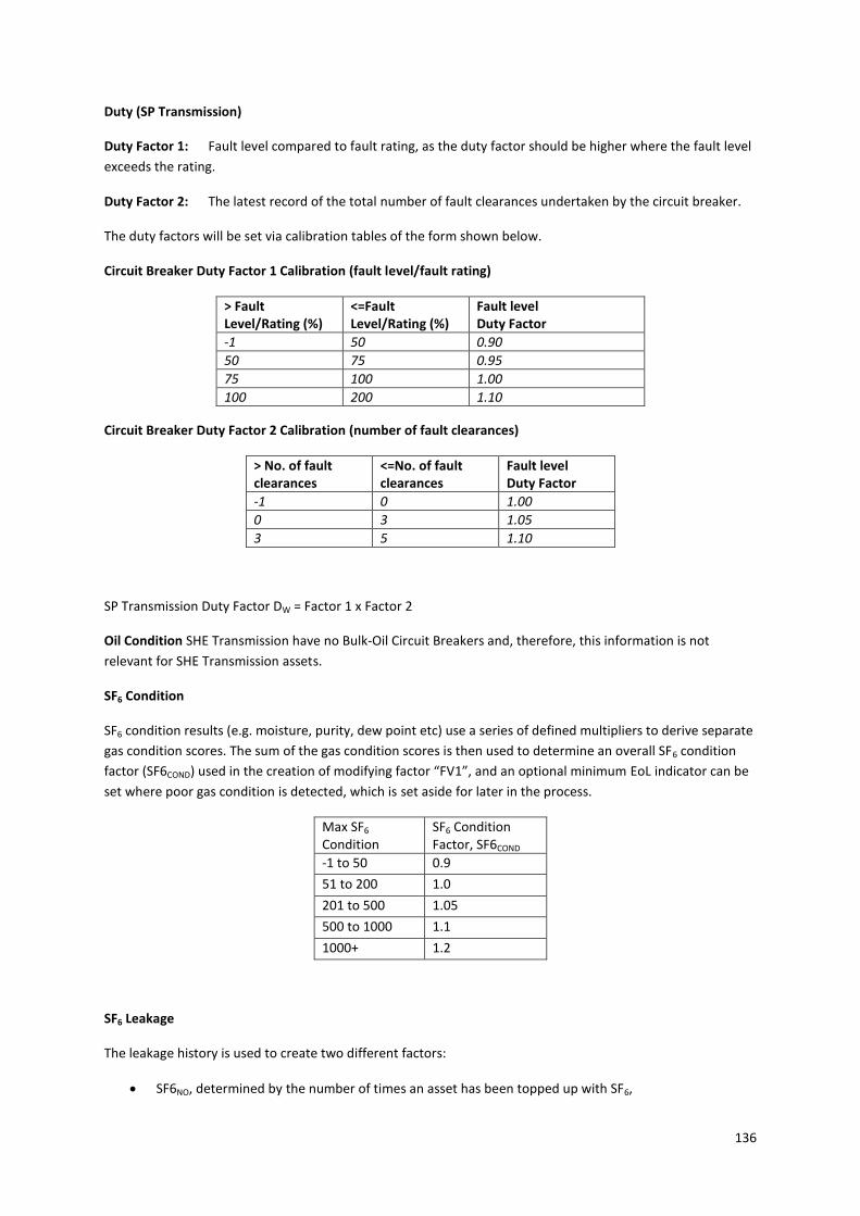
136

Duty (SP Transmission)

Duty Factor 1: Fault level compared to fault rating, as the duty factor should be higher where the fault level

exceeds the rating.

Duty Factor 2: The latest record of the total number of fault clearances undertaken by the circuit breaker.

The duty factors will be set via calibration tables of the form shown below.

Circuit Breaker Duty Factor 1 Calibration (fault level/fault rating)

> Fault Level/Rating (%)

<=Fault Level/Rating (%)

Fault level Duty Factor

-1 50 0.90

50 75 0.95

75 100 1.00

100 200 1.10

Circuit Breaker Duty Factor 2 Calibration (number of fault clearances)

> No. of fault clearances

<=No. of fault clearances

Fault level Duty Factor

-1 0 1.00

0 3 1.05

3 5 1.10

SP Transmission Duty Factor DW = Factor 1 x Factor 2

Oil Condition SHE Transmission have no Bulk-Oil Circuit Breakers and, therefore, this information is not

relevant for SHE Transmission assets.

SF6 Condition

SF6 condition results (e.g. moisture, purity, dew point etc) use a series of defined multipliers to derive separate

gas condition scores. The sum of the gas condition scores is then used to determine an overall SF6 condition

factor (SF6COND) used in the creation of modifying factor “FV1”, and an optional minimum EoL indicator can be

set where poor gas condition is detected, which is set aside for later in the process.

Max SF6

Condition SF6 Condition Factor, SF6COND

-1 to 50 0.9

51 to 200 1.0

201 to 500 1.05

500 to 1000 1.1

1000+ 1.2

SF6 Leakage

The leakage history is used to create two different factors:

SF6NO, determined by the number of times an asset has been topped up with SF6,

137

SF6LOST a second factor which considers the volume of gas replaced in relation to the weight of SF6

held by each asset by design.

Number of SF6 Leaks

SF6 Volume Factor, SF6NO

Weighted Lost SF6 SF6 Condition Factor, SF6LOST

0 1.0 0 to 0.1 1.0

1 1.1 0.1 to 0.2 1.05

2-3 1.25 0.2 to 0.5 1.1

3+ 1.5 0.5+ 1.25

A third factor can be derived from poor leakage history exception report information which reflects the TO’s

experience of loss of SF6 containment. The maximum of these 3 factors is carried forward to be included in the

EOL(2) calculation.

𝑆𝐹6𝐿𝐸𝐴𝐾 = max (𝑆𝐹6𝑁𝑂, 𝑆𝐹6𝐿𝑂𝑆𝑇)

The EOL(2) module combines the overall condition factor, defect history factor, generic reliability factor, overall

SOP factor, overall test result factor, SF6 condition factor and the SF6 leakage history factor in order to

determine modifying factor ‘FV1’. This is then multiplied with EOL(1) from the previous calculation stage to

determine EOL(2).

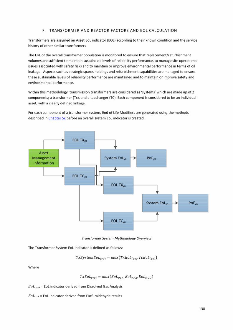
138

F. TRANSFORMER AND REACTOR FACTORS AND EOL CALCULATION

Transformers are assigned an Asset EoL indicator (EOL) according to their known condition and the service

history of other similar transformers

The EoL of the overall transformer population is monitored to ensure that replacement/refurbishment

volumes are sufficient to maintain sustainable levels of reliability performance, to manage site operational

issues associated with safety risks and to maintain or improve environmental performance in terms of oil

leakage. Aspects such as strategic spares holdings and refurbishment capabilities are managed to ensure

these sustainable levels of reliability performance are maintained and to maintain or improve safety and

environmental performance.

Within this methodology, transmission transformers are considered as ‘systems’ which are made up of 2

components; a transformer (Tx), and a tapchanger (TC). Each component is considered to be an individual

asset, with a clearly defined linkage.

For each component of a transformer system, End of Life Modifiers are generated using the methods

described in Chapter 5c before an overall system EoL indicator is created.

Transformer System Methodology Overview

The Transformer System EoL indicator is defined as follows:

𝑇𝑥𝑆𝑦𝑠𝑡𝑒𝑚𝐸𝑜𝐿(𝑦0) = 𝑚𝑎𝑥(𝑇𝑥𝐸𝑜𝐿(𝑦0), 𝑇𝑐𝐸𝑜𝐿(𝑦0))

Where

𝑇𝑥𝐸𝑜𝐿(𝑦0) = 𝑚𝑎𝑥(𝐸𝑜𝐿𝐷𝐺𝐴, 𝐸𝑜𝐿𝐹𝐹𝐴, 𝐸𝑜𝐿𝑀𝑂𝐷)

𝐸𝑜𝐿 DGA = EoL indicator derived from Dissolved Gas Analysis

𝐸𝑜𝐿 FFA = EoL indicator derived from Furfuraldehyde results


System EoLy0

EOL TXy0

PoFy0

EOL TCy0

EOL TXyn

EOL TCyn

System EoLyn PoFyn

139

𝐸𝑜𝐿 MOD = EoL indicator derived from other factors (described below) including the Initial EoL indicator.

This system EoL indicator is then used to calculate a probability of failure, PoF for a number of defined failure

modes.


Duty

For each transformer, the duty factor is calculated from the following variables:

SHE Transmission

maximum operating temperature recorded against each transformer. SHE Transmission use

this variable instead of average demand as they believe this has more impact upon the

expected life of the asset, and average demand will always be overridden by maximum

demand.

maximum demand placed upon the transformer as a percentage of its stated rating,

operational experience in the form of a ‘high duty’ exception report.

SP Transmission

maximum demand placed upon the transformer as a percentage of its stated rating,

average demand placed upon the transformer as a percentage of its stated rating,

operational experience in the form of a ‘high duty’ exception report.

Maximum Operating Temperature (Tmax) (SHE Transmission only)

A Tmax factor is determined using the following parameters:

Maximum Operating Temperature

Factor, Tmax

0 - 80 0.75

80 - 95 1.0

95 - 105 1.25

105 - 150 1.5

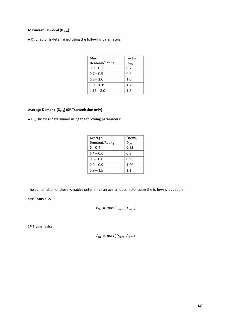
140

Maximum Demand (Dmax)

A Dmax factor is determined using the following parameters:

Max Demand/Rating

Factor Dmax

0.0 – 0.7 0.75

0.7 – 0.9 0.9

0.9 – 1.0 1.0

1.0 – 1.15 1.25

1.15 – 2.0 1.5

Average Demand (Dave) (SP Transmission only)

A Dave factor is determined using the following parameters:

Average Demand/Rating

Factor, Dave

0 – 0.4 0.85

0.4 – 0.6 0.9

0.6 – 0.8 0.95

0.8 – 0.9 1.00

0.9 – 1.5 1.1

The combination of these variables determines an overall duty factor using the following equation:

SHE Transmission

𝐹𝐷𝑌 = 𝑚𝑎𝑥(𝑇𝑚𝑎𝑥 , 𝐷𝑚𝑎𝑥)

SP Transmission

𝐹𝐷𝑌 = 𝑚𝑎𝑥(𝐷𝑚𝑎𝑥 , 𝐷𝑎𝑣𝑒)

141

Situation Factor (SP Transmission)

The situation factor is determined based upon the following table;

Situation Factor

Outdoor 1.00

Indoor 0.90

Noise Enclosure 1.00

Completely Enclosed 0.95

Main Tank Enclosed only 0.95

Situation Factor (SHE Transmission)

The situation factor is determined based upon the following table;

Situation Factor

Outdoor 1.00

Indoor 0.5

These factors are larger than that for SP Transmission to reflect the harsher environment imposed on many of

SHE Transmission’s assets in the Highlands and Islands of Scotland.

Oil Condition

Established techniques such as oil analysis provide an effective means of identifying and quantifying

degradation of the insulation system (oil and paper) within transformers. Oil results can also be used to

identify incipient faults. The oil condition factor considers the latest oil condition tests, (moisture, acidity,

breakdown strength and tan delta) each of which is used to create a test score.

Relative Humidity (%)

Moisture Score

Breakdown Voltage (kV)

Breakdown Strength Score

0 - 15 0 0 - 30 20

15 - 30 2 30 - 40 6

30 - 50 4 40 - 50 2

50 - 65 8 50 - 10000 0

65 – 500 20

Tan Delta @90°C

Tan Delta Score

Acidity – mg KOH/g

Acidity Score

0 – 0.02 0 0 – 0.03 0

0.02 – 0.06 2 0.03 – 0.075 2

0.06 – 0.12 4 0.075 - 0.15 4

0.12 – 0.2 8 0.15 - 0.25 8

0.2 - 1 20 0.25 - 2 20

142

Each of these scores is given a multiplier which accounts for the significance of the result:

Test Multiplier

Relative Humidity 80

Breakdown Voltage (kV) 80

Tan Delta @90°C 80

Acidity – mg KOH/g 125

The summation of the individual oil condition test scores is then used to determine an overall oil condition

factor.

Oil Condition Score

Factor, FOIL

0 – 200 0.75

200 – 500 1.0

500 – 950 1.1

950 – 1500

1.25

1500+ 1.5

The EOL(2) module combines the overall condition factor, defect history factor, family reliability factor, overall

test result factor, overall OR factor and the overall oil condition score in order to determine modifying factor

‘FV1’. This is then multiplied by EOL(1) to determine EOL(2).

Derivation of Tx EOL(DGA)

EOL(DGA) is derived from the dissolved gas analysis (DGA) oil test results. This is a very well established process

that enables abnormal electrical or thermal activity to be detected by measurement of hydrogen and

hydrocarbon gases that are breakdown products of the oil. The levels and combination of gases enable

detection of developing faults and identification of 'life threatening' conditions.

Each oil sample is analysed for levels of Hydrogen, Acetylene, Ethane, Ethylene, Methane, Oxygen and

Nitrogen which provide indications of the internal condition of the transformer. The rate of change of DGA

values is also considered so as to take into account each transformer’s historical test results. The boundaries

for assessment of DGA levels are taken from the Cigre Working Group 15.01 paper, “New guidelines for

interpretation of dissolved gas analysis in oil-filled transformers”. These boundaries can provide useful

information relating to incipient faults within transformers or contamination of the main tank oil from the

tapchanger. The parameters used to derive EOL(DGA) are listed in the tables below:

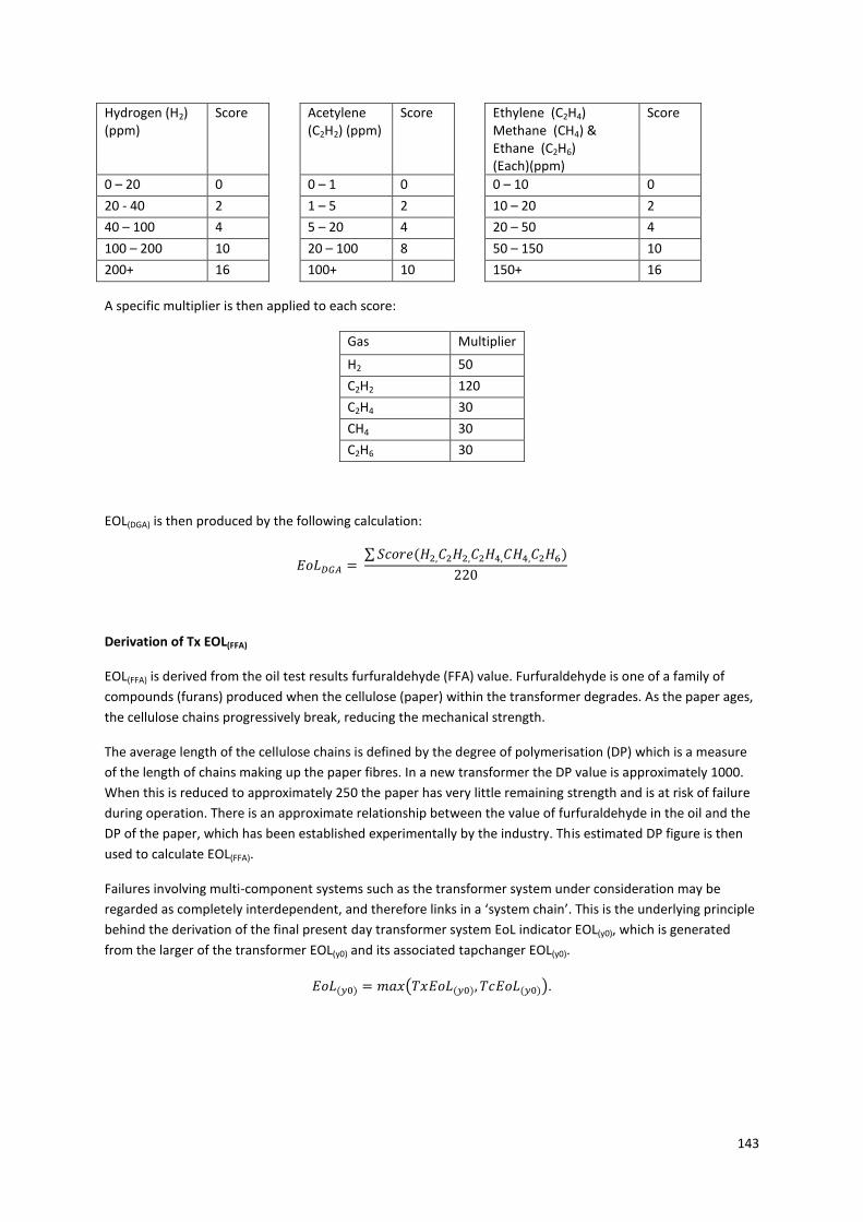
143

Hydrogen (H2) (ppm)

Score Acetylene (C2H2) (ppm)

Score Ethylene (C2H4) Methane (CH4) & Ethane (C2H6) (Each)(ppm)

Score

0 – 20 0 0 – 1 0 0 – 10 0

20 - 40 2 1 – 5 2 10 – 20 2

40 – 100 4 5 – 20 4 20 – 50 4

100 – 200 10 20 – 100 8 50 – 150 10

200+ 16 100+ 10 150+ 16

A specific multiplier is then applied to each score:

Gas Multiplier

H2 50

C2H2 120

C2H4 30

CH4 30

C2H6 30

EOL(DGA) is then produced by the following calculation:

𝐸𝑜𝐿𝐷𝐺𝐴 = ∑ 𝑆𝑐𝑜𝑟𝑒(𝐻2,𝐶2𝐻2,𝐶2𝐻4,𝐶𝐻4,𝐶2𝐻6)

220

Derivation of Tx EOL(FFA)

EOL(FFA) is derived from the oil test results furfuraldehyde (FFA) value. Furfuraldehyde is one of a family of

compounds (furans) produced when the cellulose (paper) within the transformer degrades. As the paper ages,

the cellulose chains progressively break, reducing the mechanical strength.

The average length of the cellulose chains is defined by the degree of polymerisation (DP) which is a measure

of the length of chains making up the paper fibres. In a new transformer the DP value is approximately 1000.

When this is reduced to approximately 250 the paper has very little remaining strength and is at risk of failure

during operation. There is an approximate relationship between the value of furfuraldehyde in the oil and the

DP of the paper, which has been established experimentally by the industry. This estimated DP figure is then

used to calculate EOL(FFA).

Failures involving multi-component systems such as the transformer system under consideration may be

regarded as completely interdependent, and therefore links in a ‘system chain’. This is the underlying principle

behind the derivation of the final present day transformer system EoL indicator EOL(y0), which is generated

from the larger of the transformer EOL(y0) and its associated tapchanger EOL(y0).

𝐸𝑜𝐿(𝑦0) = 𝑚𝑎𝑥(𝑇𝑥𝐸𝑜𝐿(𝑦0), 𝑇𝑐𝐸𝑜𝐿(𝑦0)).

144

G. UNDERGROUND CABLE FACTORS AND EOL CALCULATION

Cables are assigned an Asset EoL indicator (EOL) according to their known condition and the service history of

other similar cables.

Within this methodology, transmission cables are considered as number of discrete cable lengths (or

‘component’) which together form a distinct circuit.

For each component of cable circuit asset management information is fed into the model in order to produce a

component EoL indicator, referred to as EOL(Y0), before an overall system EoL indicator is created. This system

EoL indicator is then used to calculate a probability of failure, PoF for a number of defined failure modes.

There are three separate models within the main underground cable model reflecting the following types of

construction;

Oil

Non-pressurised

Submarine cable

Each model uses a similar format, though certain condition points are ‘construction’ dependent and only used

within that model as a factor.

The models contain an ageing mechanism, which attempts to estimate the likely future EoL indices for each

cable to as EOL(yn). These future EOL estimations are combined in an identical fashion to the present day EOL

calculation, so as to derive an overall cable future EOL, and it is this which is used to project future PoF of each

of the cables being considered.


Duty

For each cable, the duty factor is calculated based upon the following variables:

SP Transmission

maximum demand placed on the cable as a percentage of its rating.

average load on the cable as a percentage of its rating.

operating voltage compared to the design voltage exception report

High Circulating Current exception report

SHE Transmission

maximum demand placed on the cable as a percentage of its rating.

connection to reactive earthing

145

SHE Transmission do not use average demand as it will always be overridden by maximum demand.

As the effects of utilisation vary between cable types, separate duty factors will be established for each cable

type. This classification will be based upon insulation type.

Maximum Demand (Dmax)

A Dmax factor is determined using the following parameters:

Maximum Demand/Rating

Factor, Dmax

0 - 80 0.75

80 - 95 1.0

95 - 105 1.25

105 - 150 1.5

Average Demand (Dave) (SP Transmission only)

A Dave factor is determined using the following parameters:

Max Demand/Rating

Factor Dave

0.0 – 0.7 0.75

0.7 – 0.9 0.9

0.9 – 1.0 1.0

1.0 – 1.15 1.25

1.15 – 2.0 1.5

Reactive Earthing (SHE Transmission Only)

Reactive Earting/Peterson Coil Cct

Factor DRE

No 1.0

Yes 1.2

The combination of these three variables determines an overall duty factor using the following equation:

FDY = max(Dmax, Dave , DRE)

146


For each cable the LSE factor is calculated from a situation factor and an installation factor, as shown in Figure

2 below.

LSE factor

The installation factor for oil and non-pressurised cables is based upon the following variables:

As laid depth (FD)

As laid configuration (FC) (SP Transmission Only)

Ploughed Installation Factor(Fl) (SHE Transmission Only)

SHE Transmission uses a Ploughed Installation Factor rather than Backfill material as the majority of our cables

are ploughed and, therefore, have no backfill material.

As laid depth/Shallow ducts

A depth factor is determined using the following parameters:

As laid depth (m) Factor, FD

0 -5 1.35

5 – 10 1.2

10 – 15 1.1

15 – 20 1.0

20 – 25 0.9

25+ 0.85

As laid configuration

A configuration factor is determined using the following parameters:

As laid Configuration

Factor, FC

Flat 1

Laid Direct 1

Trefoil 1.0

Unknown 0.9

Ploughed Installation Factor

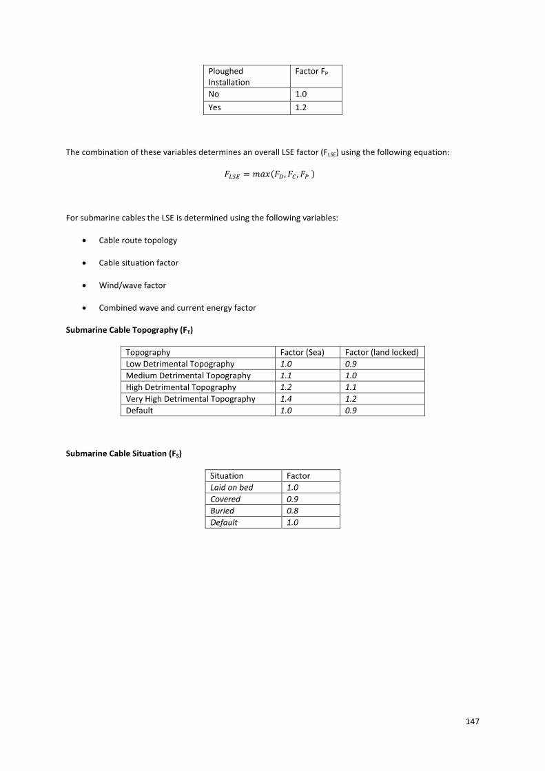
147

Ploughed Installation

Factor FP

No 1.0

Yes 1.2

The combination of these variables determines an overall LSE factor (FLSE) using the following equation:

𝐹𝐿𝑆𝐸 = 𝑚𝑎𝑥(𝐹𝐷 , 𝐹𝐶 , 𝐹𝑃 )

For submarine cables the LSE is determined using the following variables:

Cable route topology

Cable situation factor

Wind/wave factor

Combined wave and current energy factor

Submarine Cable Topography (FT)

Topography Factor (Sea) Factor (land locked)

Low Detrimental Topography 1.0 0.9

Medium Detrimental Topography 1.1 1.0

High Detrimental Topography 1.2 1.1

Very High Detrimental Topography 1.4 1.2

Default 1.0 0.9

Submarine Cable Situation (FS)

Situation Factor

Laid on bed 1.0

Covered 0.9

Buried 0.8

Default 1.0

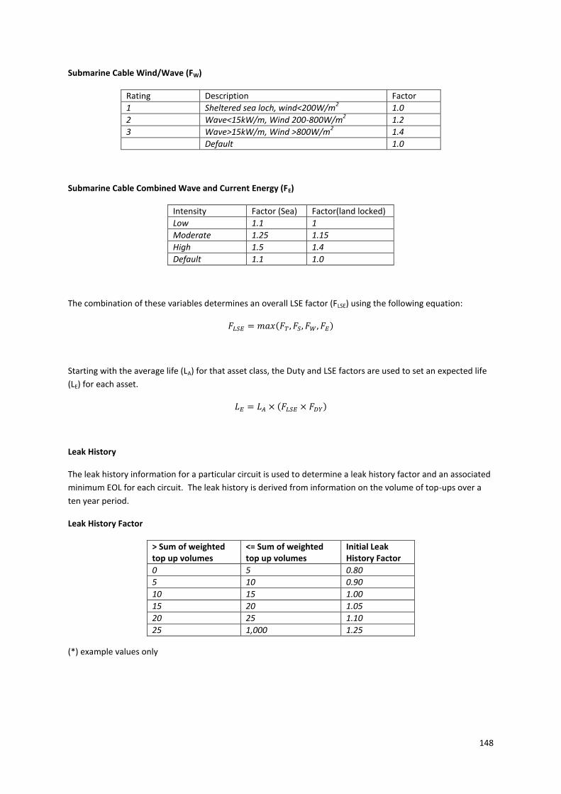
148

Submarine Cable Wind/Wave (FW)

Rating Description Factor

1 Sheltered sea loch, wind<200W/m2

1.0

2 Wave<15kW/m, Wind 200-800W/m2 1.2

3 Wave>15kW/m, Wind >800W/m2 1.4

Default 1.0

Submarine Cable Combined Wave and Current Energy (FE)

Intensity Factor (Sea) Factor(land locked)

Low 1.1 1

Moderate 1.25 1.15

High 1.5 1.4

Default 1.1 1.0

The combination of these variables determines an overall LSE factor (FLSE) using the following equation:

𝐹𝐿𝑆𝐸 = 𝑚𝑎𝑥(𝐹𝑇 , 𝐹𝑆, 𝐹𝑊 , 𝐹𝐸)



𝐿𝐸 = 𝐿𝐴 × (𝐹𝐿𝑆𝐸 × 𝐹𝐷𝑌)

Leak History

The leak history information for a particular circuit is used to determine a leak history factor and an associated

minimum EOL for each circuit. The leak history is derived from information on the volume of top-ups over a

ten year period.

Leak History Factor

> Sum of weighted top up volumes

<= Sum of weighted top up volumes

Initial Leak History Factor

0 5 0.80

5 10 0.90

10 15 1.00

15 20 1.05

20 25 1.10

25 1,000 1.25

(*) example values only

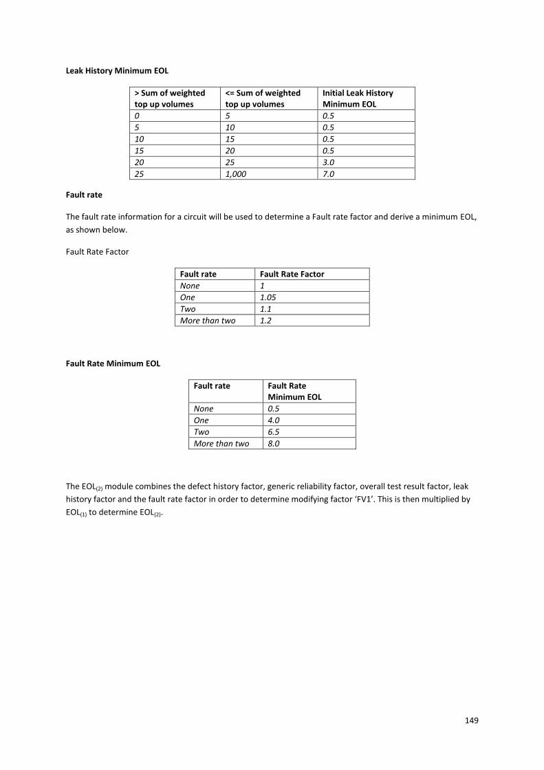
149

Leak History Minimum EOL

> Sum of weighted top up volumes

<= Sum of weighted top up volumes

Initial Leak History Minimum EOL

0 5 0.5

5 10 0.5

10 15 0.5

15 20 0.5

20 25 3.0

25 1,000 7.0

Fault rate

The fault rate information for a circuit will be used to determine a Fault rate factor and derive a minimum EOL,

as shown below.

Fault Rate Factor

Fault rate Fault Rate Factor

None 1

One 1.05

Two 1.1

More than two 1.2

Fault Rate Minimum EOL

Fault rate Fault Rate Minimum EOL

None 0.5

One 4.0

Two 6.5

More than two 8.0

The EOL(2) module combines the defect history factor, generic reliability factor, overall test result factor, leak

history factor and the fault rate factor in order to determine modifying factor ‘FV1’. This is then multiplied by

EOL(1) to determine EOL(2).

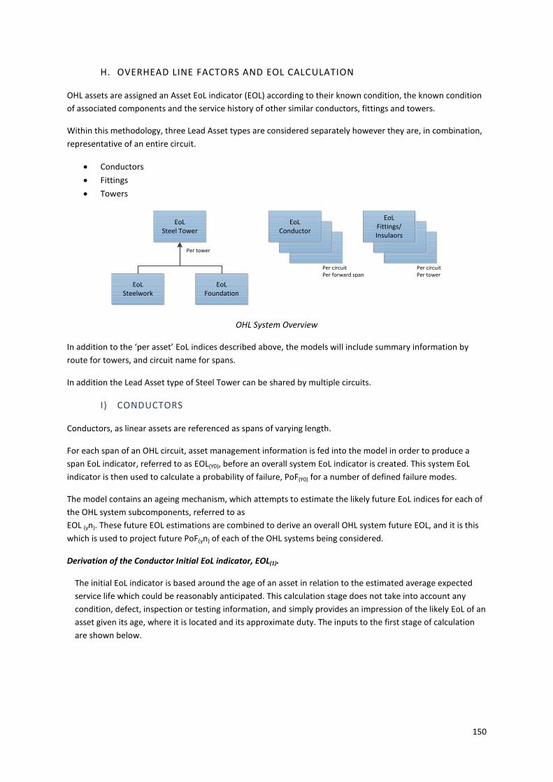
150

H. OVERHEAD LINE FACTORS AND EOL CALCULATION

OHL assets are assigned an Asset EoL indicator (EOL) according to their known condition, the known condition

of associated components and the service history of other similar conductors, fittings and towers.

Within this methodology, three Lead Asset types are considered separately however they are, in combination,

representative of an entire circuit.

Conductors

Fittings

Towers

OHL System Overview

In addition to the ‘per asset’ EoL indices described above, the models will include summary information by

route for towers, and circuit name for spans.

In addition the Lead Asset type of Steel Tower can be shared by multiple circuits.

I) CONDUCTORS

Conductors, as linear assets are referenced as spans of varying length.

For each span of an OHL circuit, asset management information is fed into the model in order to produce a

span EoL indicator, referred to as EOL(Y0), before an overall system EoL indicator is created. This system EoL

indicator is then used to calculate a probability of failure, PoF(Y0) for a number of defined failure modes.

The model contains an ageing mechanism, which attempts to estimate the likely future EoL indices for each of

the OHL system subcomponents, referred to as

EOL (yn). These future EOL estimations are combined to derive an overall OHL system future EOL, and it is this

which is used to project future PoF(yn) of each of the OHL systems being considered.

Derivation of the Conductor Initial EoL indicator, EOL(1).




asset given its age, where it is located and its approximate duty. The inputs to the first stage of calculation

are shown below.

EoL Steel Tower

EoL Conductor

EoL Fittings/Insulaors

EoL Steelwork

EoL Foundation

Per tower

Per circuitPer forward span

Per circuitPer tower

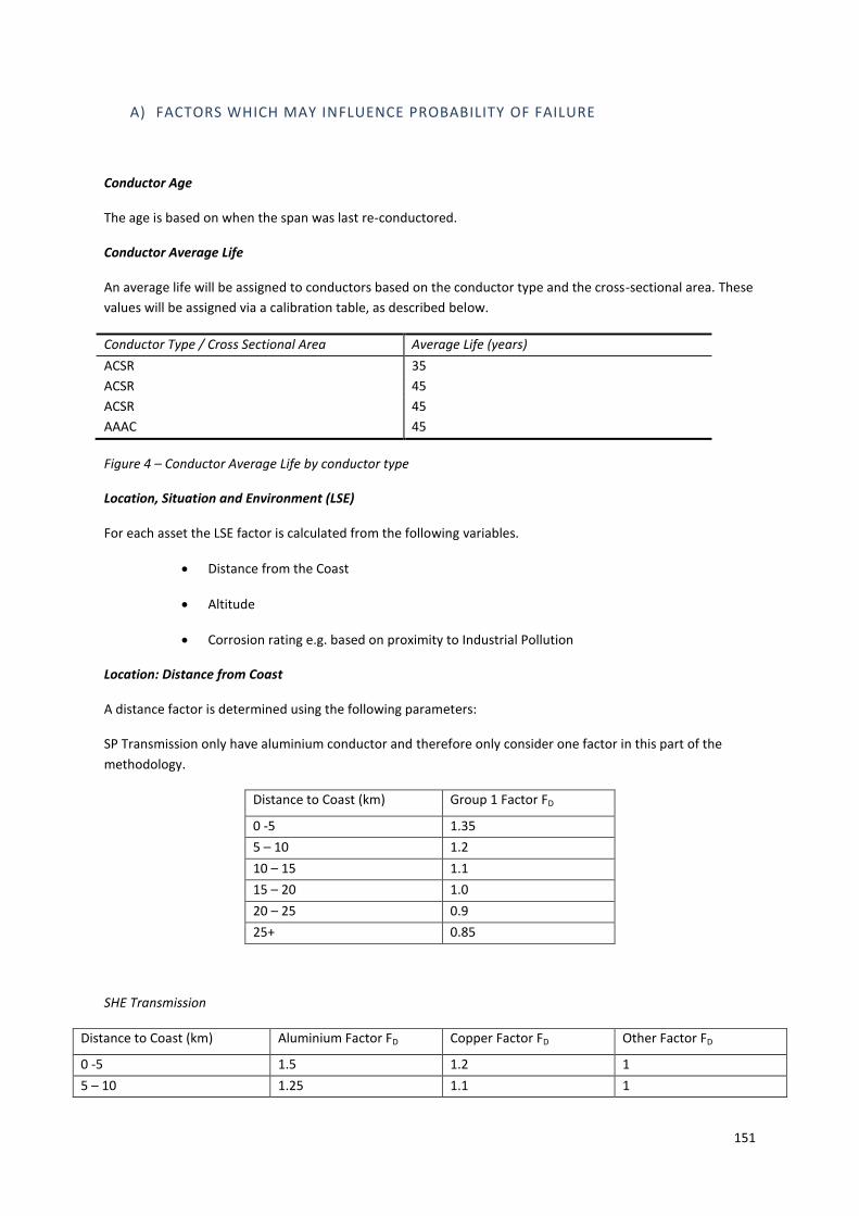
151


Conductor Age

The age is based on when the span was last re-conductored.

Conductor Average Life

An average life will be assigned to conductors based on the conductor type and the cross-sectional area. These

values will be assigned via a calibration table, as described below.

Conductor Type / Cross Sectional Area Average Life (years)

ACSR 35

ACSR 45

ACSR 45

AAAC 45

Figure 4 – Conductor Average Life by conductor type


For each asset the LSE factor is calculated from the following variables.

Distance from the Coast

Altitude

Corrosion rating e.g. based on proximity to Industrial Pollution

Location: Distance from Coast


SP Transmission only have aluminium conductor and therefore only consider one factor in this part of the

methodology.

Distance to Coast (km) Group 1 Factor FD

0 -5 1.35

5 – 10 1.2

10 – 15 1.1

15 – 20 1.0

20 – 25 0.9

25+ 0.85

SHE Transmission

Distance to Coast (km) Aluminium Factor FD Copper Factor FD Other Factor FD

0 -5 1.5 1.2 1

5 – 10 1.25 1.1 1

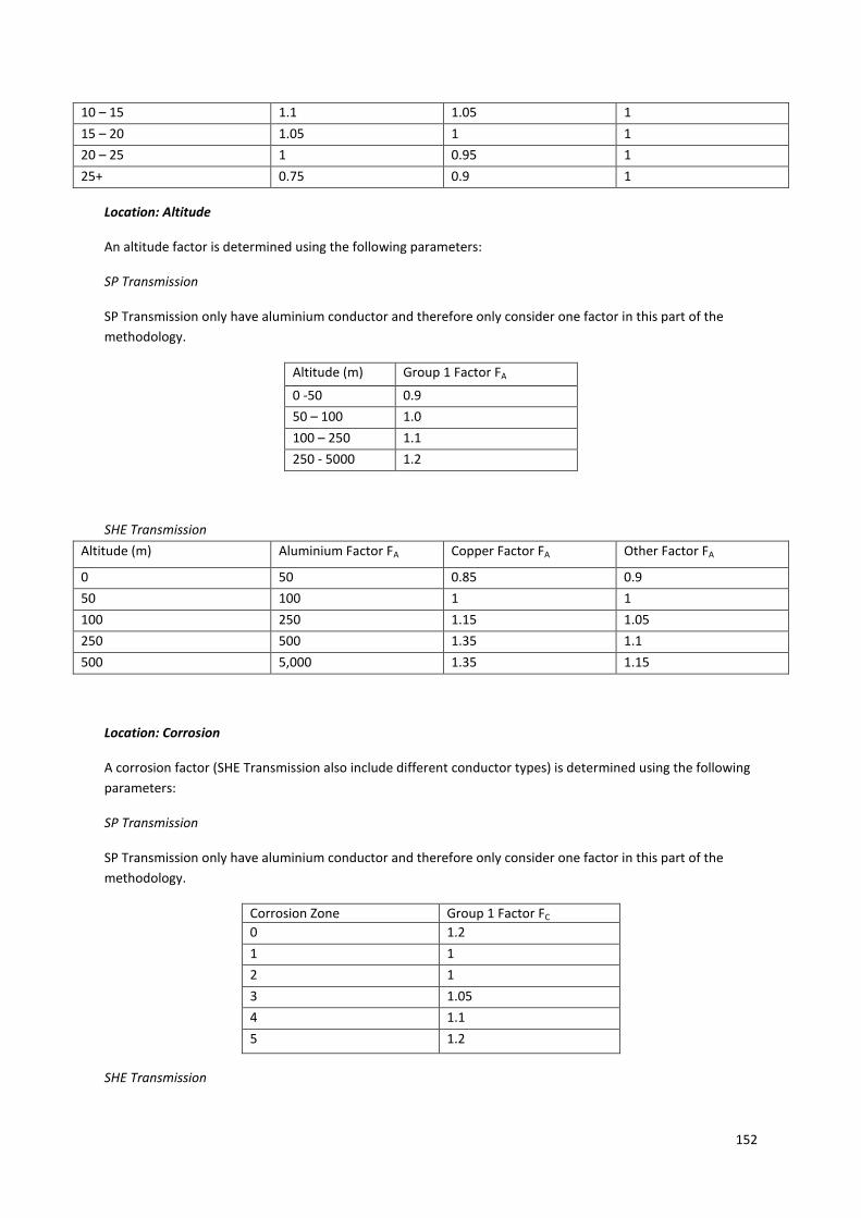
152

10 – 15 1.1 1.05 1

15 – 20 1.05 1 1

20 – 25 1 0.95 1

25+ 0.75 0.9 1

Location: Altitude


SP Transmission


methodology.

Altitude (m) Group 1 Factor FA

0 -50 0.9

50 – 100 1.0

100 – 250 1.1

250 - 5000 1.2

SHE Transmission

Altitude (m) Aluminium Factor FA Copper Factor FA Other Factor FA

0 50 0.85 0.9

50 100 1 1

100 250 1.15 1.05

250 500 1.35 1.1

500 5,000 1.35 1.15

Location: Corrosion

A corrosion factor (SHE Transmission also include different conductor types) is determined using the following

parameters:

SP Transmission


methodology.

Corrosion Zone Group 1 Factor FC

0 1.2

1 1

2 1

3 1.05

4 1.1

5 1.2

SHE Transmission

153

Corrosion Zone Aluminium Factor FC Copper Factor FC Other Factor FC

1 0.75 0.9 1

2 1 0.95 1

3 1 1 1

4 1.25 1.1 1

5 1.5 1.2 1

154

The combination of these three variables determines an overall LSE factor (FL) using the following equation:

𝐹𝐿 = 𝑚𝑎𝑥(𝐹𝐷, 𝐹𝐴, 𝐹𝐶)

Environment

Environment also is a degrading factor for example if the conductor is in an area known to experience severe

weather.

SP Transmission

As previously mentioned , SP Transmission only have aluminium conductor and therefore only consider one

factor in this part of the methodology.

Environmental Rating Environmental Factor

Bad 1.1

Poor 1.2

SHE Transmission

Severe Weather Zone Aluminium Copper Other

Bad 1.3 1.3 1

Normal 1 1 1

Poor 1.1 1.1 1

The overall LSE factor is derived using the following equation:

LSE Factor = ((Location Factor – Min. Possible Location Factor) x Situation Factor) + Min Possible Location

Factor) x Environment Factor



𝑳𝑬 = 𝑳𝑨 × 𝑭𝑳𝑺𝑬

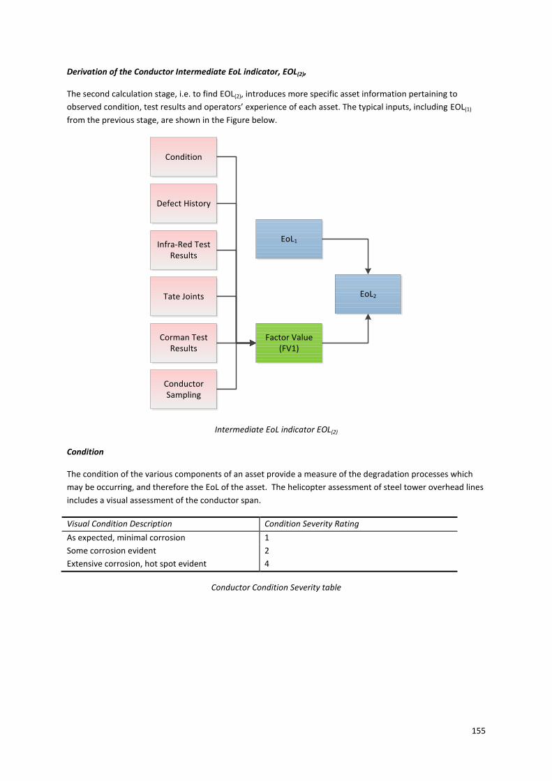
155

Derivation of the Conductor Intermediate EoL indicator, EOL(2),


observed condition, test results and operators’ experience of each asset. The typical inputs, including EOL(1)

from the previous stage, are shown in the Figure below.

Intermediate EoL indicator EOL(2)

Condition

The condition of the various components of an asset provide a measure of the degradation processes which

may be occurring, and therefore the EoL of the asset. The helicopter assessment of steel tower overhead lines

includes a visual assessment of the conductor span.

Visual Condition Description Condition Severity Rating

As expected, minimal corrosion 1

Some corrosion evident 2

Extensive corrosion, hot spot evident 4

Conductor Condition Severity table

Condition

Defect History

Infra-Red Test Results

Tate Joints

Corman Test Results

Conductor Sampling

Factor Value (FV1)

EoL1

EoL2

156

Defect History

The number of defects experienced on the span over the previous 5 years (including those that have been

repaired are identified. Each defect will then be assigned a severity rating (using a scale of 1 to 4, where 4 is

the most severe) via a calibration table.

Defect Description Defect Severity Rating

Description 1 1

Description 2 2

Description 3 4

Conductor Defect Calibration Table

Infra-red Test Results

Helicopter inspections of the Over Head Lines are used to identify hot joints on conductors. This information

will be used to derive an infra-red test factor and a minimum EOL value via calibration tables as shown below.

Where tests have been undertaken, the results (either pass, suspect or fail) for each test type are used to

derive individual test factors (and if desired minimum EoL indices) and are then combined in order to produce

an overall test factor. The overall test factor is included in the formation of modifying factor FV1, while any

defined minimum EoL indices are set aside for use later in the process.

Infra-Red

Results

Infra-Red Test Factor Infra-Red Results Infra-Red Test

Minimum EOL

Pass 1.0 Pass 0.5

Fail 1.2 Fail 7.0

Infra Red Test Factor and Min EOL Calibration

Tate Joints (SHE Transmission Only)

A Tate joint factor is applied to conductor spans where Tate joints are present. This module also has the facility

to set minimum a EOL for spans where Tate joints are identified.

Tate Joints Tate Joints Factor

No 1

Yes 1.2

Tate Joint Factor Calibration

Currently SP Transmission do not have this factor modelled within their methodology, but will undertake as

assessment of whether this should be included as we progress through the implementation period.

157

Cormon Test Results

Cormon testing measures the extent of corrosion on ACSR conductors, and can be used to derive a EoL

indicator independently of any other information on condition or age.

The test results are used to derive a Cormon EoL indicator via a calibration table of the form shown below.

The tests are conducted on a span or number of spans and the results are then applied to the whole circuit.

The test results are converted to a score, e.g. 1-4.

Cormon Score Cormon EOL

1 2

2 3

3 4

4 5

Cormon Score EoL Indicator

Conductor Sampling

Conductor sampling determines the extent of corrosion a sample of the overhead conductor, which is

considered to provide a representative indication of the EoL of the circuit. The results can be used to derive a

EoL indicator independently of any other information on condition or age.

The test results are used to derive a Conductor Sampling EoL indicator via a calibration table of the form

shown below. The tests results are conducted on a span or number of spans and then applied to the whole

circuit. The test results are converted to a score, e.g. 1-5.

Conductor Sampling Score Conductor Sampling EOL

1 2

2 3

3 4

4 5

5 5

Figure 15 – Conductor Sampling EoL indicator

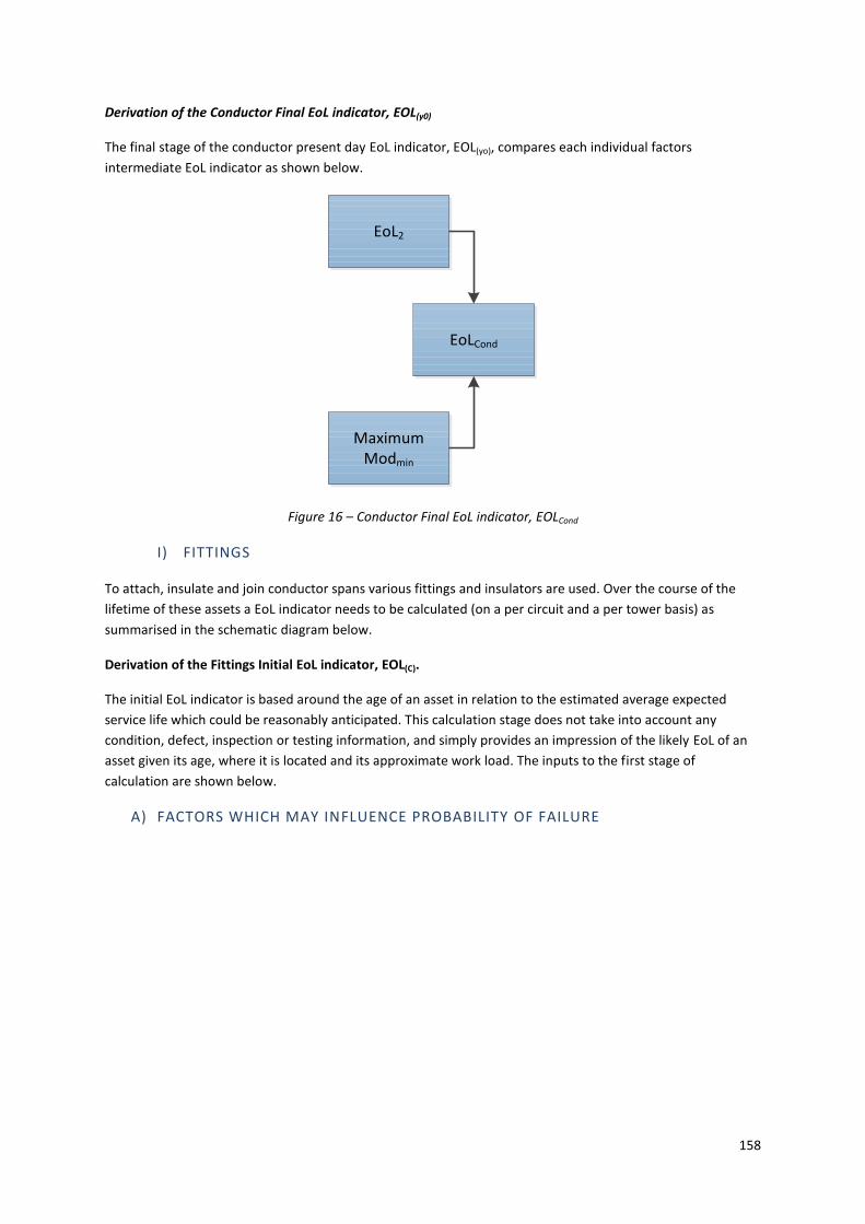
158

Derivation of the Conductor Final EoL indicator, EOL(y0)

The final stage of the conductor present day EoL indicator, EOL(yo), compares each individual factors

intermediate EoL indicator as shown below.

Figure 16 – Conductor Final EoL indicator, EOLCond

I) FITTINGS

To attach, insulate and join conductor spans various fittings and insulators are used. Over the course of the

lifetime of these assets a EoL indicator needs to be calculated (on a per circuit and a per tower basis) as

summarised in the schematic diagram below.

Derivation of the Fittings Initial EoL indicator, EOL(C).




asset given its age, where it is located and its approximate work load. The inputs to the first stage of

calculation are shown below.


Maximum Modmin

EoL2

EoLCond

159

Asset Average Life

An average life will be assigned to the fittings based on the type of insulators (i.e. glass, polymeric or

porcelain), whether they are tension/suspension fittings and the operating voltage, as highlighted below. SHE

Transmission only use suspension or tension as fitting type (not material)

Fitting Type Voltage Average Life (years)

Glass - Suspension 33 35

Porcelain - Suspension 33 45

Polymeric – Suspension 33 45

Glass – Tension 33 45

Porcelain – Tension 33

Polymeric – Tension 33

Glass - Suspension 132

Porcelain - Suspension 132

Polymeric – Suspension 132

Glass – Tension 132






Glass - Tension 275

Porcelain - Tension 275





Glass – Tension 400



Fitting Average Life by conductor type


For each asset the LSE factor is calculated from the following variables.

Distance from the Coast

Altitude

Corrosion rating e.g. based on proximity to Industrial Pollution

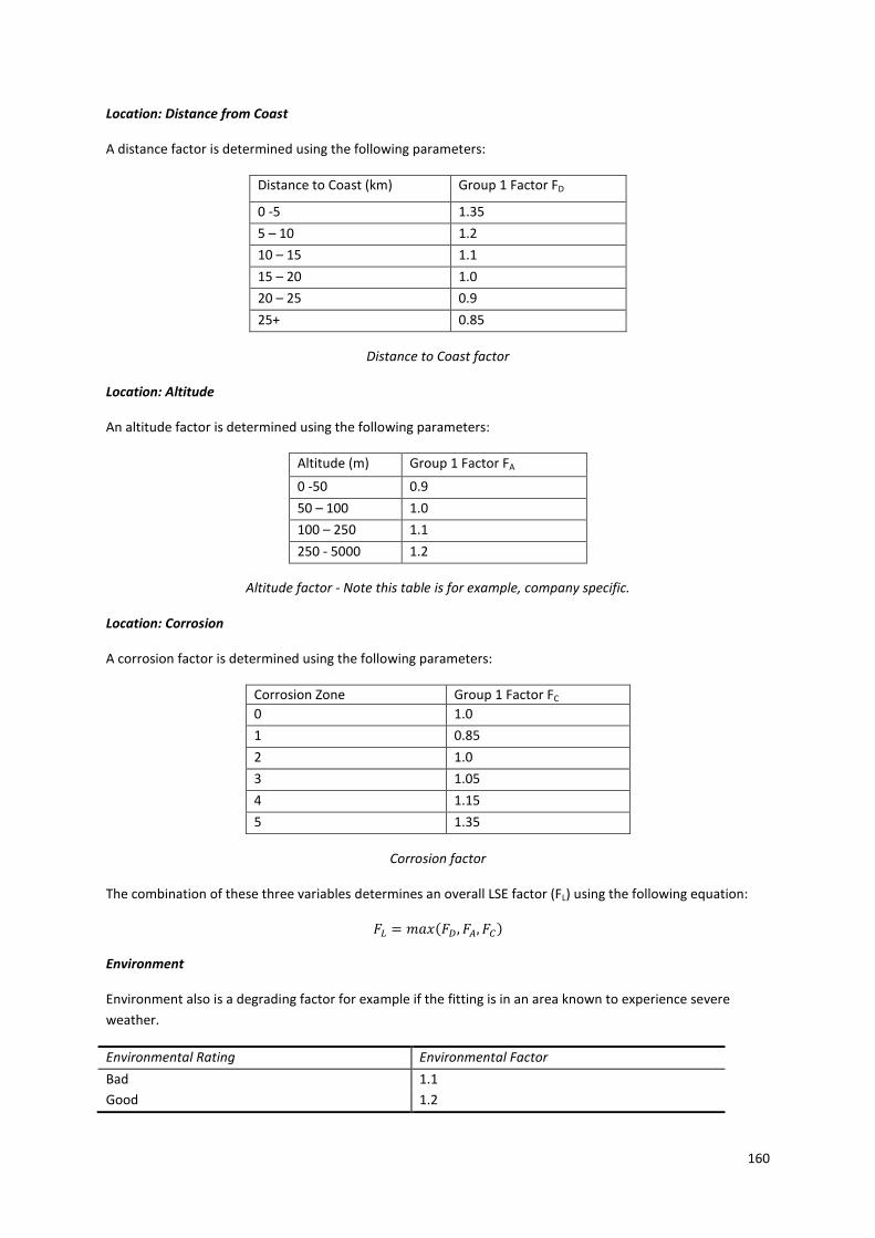
160

Location: Distance from Coast


Distance to Coast (km) Group 1 Factor FD

0 -5 1.35

5 – 10 1.2

10 – 15 1.1

15 – 20 1.0

20 – 25 0.9

25+ 0.85

Distance to Coast factor

Location: Altitude


Altitude (m) Group 1 Factor FA

0 -50 0.9

50 – 100 1.0

100 – 250 1.1

250 - 5000 1.2

Altitude factor - Note this table is for example, company specific.

Location: Corrosion

A corrosion factor is determined using the following parameters:

Corrosion Zone Group 1 Factor FC

0 1.0

1 0.85

2 1.0

3 1.05

4 1.15

5 1.35

Corrosion factor

The combination of these three variables determines an overall LSE factor (FL) using the following equation:

𝐹𝐿 = 𝑚𝑎𝑥(𝐹𝐷, 𝐹𝐴, 𝐹𝐶)

Environment

Environment also is a degrading factor for example if the fitting is in an area known to experience severe

weather.

Environmental Rating Environmental Factor

Bad 1.1

Good 1.2

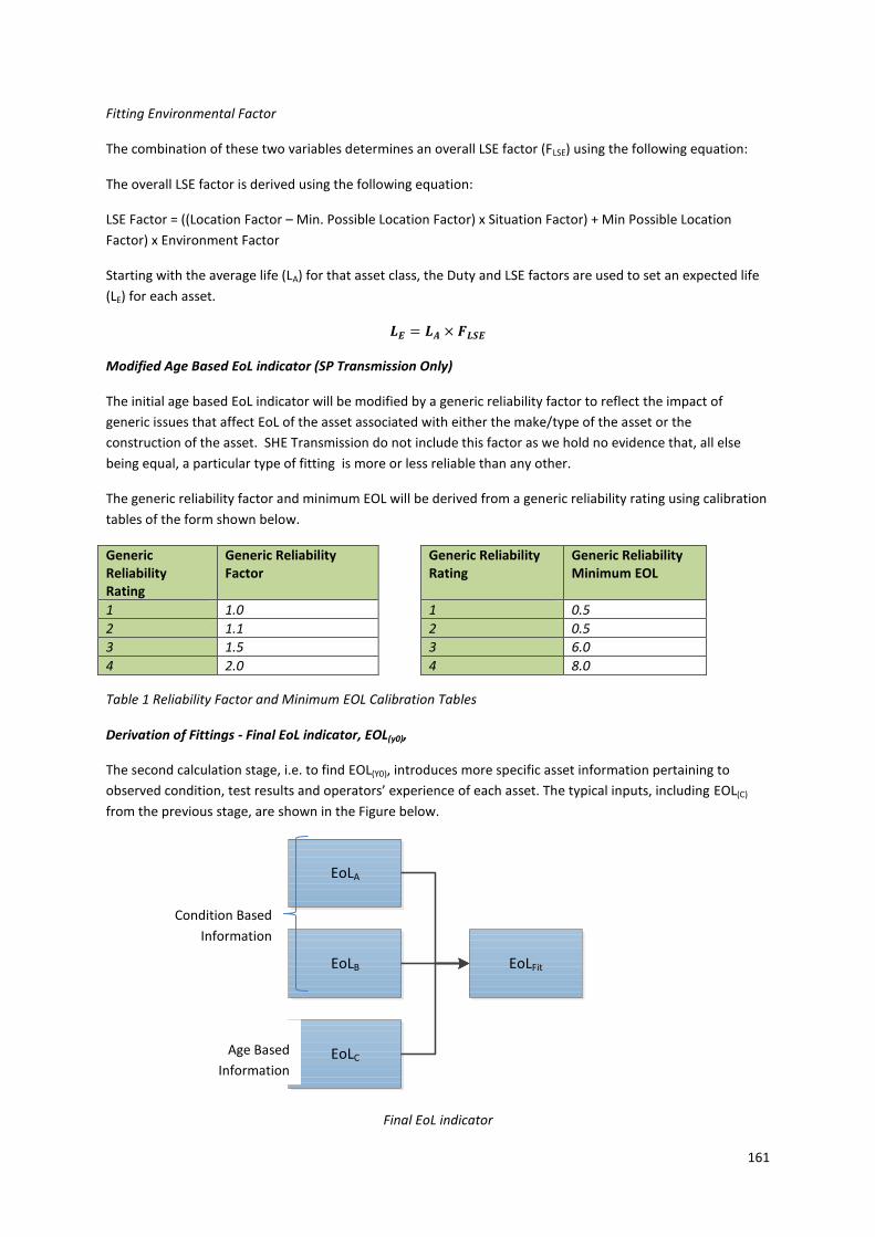
161

Fitting Environmental Factor

The combination of these two variables determines an overall LSE factor (FLSE) using the following equation:

The overall LSE factor is derived using the following equation:

LSE Factor = ((Location Factor – Min. Possible Location Factor) x Situation Factor) + Min Possible Location

Factor) x Environment Factor



𝑳𝑬 = 𝑳𝑨 × 𝑭𝑳𝑺𝑬

Modified Age Based EoL indicator (SP Transmission Only)

The initial age based EoL indicator will be modified by a generic reliability factor to reflect the impact of

generic issues that affect EoL of the asset associated with either the make/type of the asset or the

construction of the asset. SHE Transmission do not include this factor as we hold no evidence that, all else

being equal, a particular type of fitting is more or less reliable than any other.

The generic reliability factor and minimum EOL will be derived from a generic reliability rating using calibration

tables of the form shown below.

Generic Reliability Rating

Generic Reliability Factor

Generic Reliability Rating

Generic Reliability Minimum EOL

1 1.0 1 0.5

2 1.1 2 0.5

3 1.5 3 6.0

4 2.0 4 8.0

Table 1 Reliability Factor and Minimum EOL Calibration Tables

Derivation of Fittings - Final EoL indicator, EOL(y0),

The second calculation stage, i.e. to find EOL(Y0), introduces more specific asset information pertaining to

observed condition, test results and operators’ experience of each asset. The typical inputs, including EOL(C)

from the previous stage, are shown in the Figure below.

Final EoL indicator

EoLA

EoLFitEoLB

EoLC

Condition Based

Information

Age Based

Information

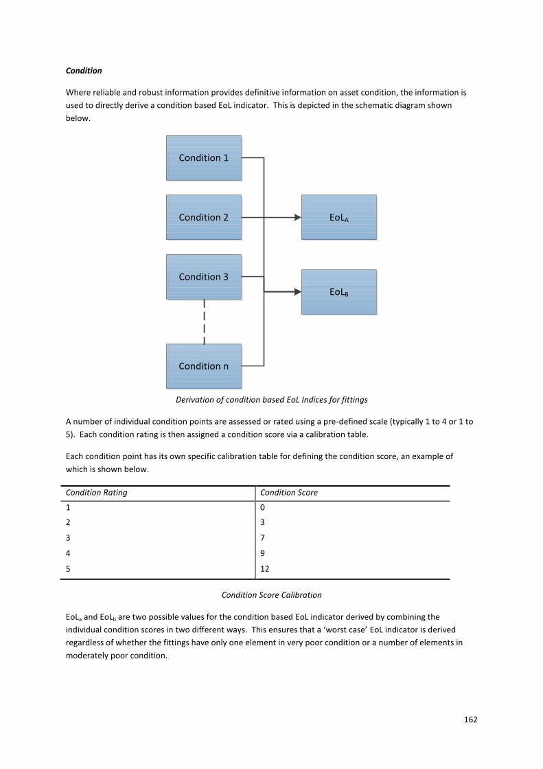
162

Condition

Where reliable and robust information provides definitive information on asset condition, the information is

used to directly derive a condition based EoL indicator. This is depicted in the schematic diagram shown

below.

Derivation of condition based EoL Indices for fittings

A number of individual condition points are assessed or rated using a pre-defined scale (typically 1 to 4 or 1 to

5). Each condition rating is then assigned a condition score via a calibration table.

Each condition point has its own specific calibration table for defining the condition score, an example of

which is shown below.

Condition Rating Condition Score

1 0

2 3

3 7

4 9

5 12

Condition Score Calibration

EoLa and EoLb are two possible values for the condition based EoL indicator derived by combining the

individual condition scores in two different ways. This ensures that a ‘worst case’ EoL indicator is derived

regardless of whether the fittings have only one element in very poor condition or a number of elements in

moderately poor condition.

Condition 1

EoLACondition 2

Condition 3

Condition n

EoLB

163

EoLa is the highest of the condition scored divided by a calibration value, whilst HIb is the sum of the three

highest condition scores divided by a second calibration value. Where condition scores are not provided, a

default condition score is applied.

Example values for the divisors and default condition scores are shown below.

Condition Rating Condition Divisor

EOLA Divisor 1.8

EoLB Divisor 5

Condition Score 1 Default 2

Condition Score 2 Default 2

Condition Score Divisors

III) TOWERS

The steel tower EoL indicator is formed from a combination of a steelwork EOL and a tower foundation EoL

indices.

The Tower EoL indicator is defined as follows:

𝐸𝑜𝐿(𝑇) = 𝑤𝑒𝑖𝑔ℎ𝑡𝑒𝑑 𝑎𝑣𝑒𝑟𝑎𝑔𝑒(𝑇𝑜𝑤𝑒𝑟 𝑆𝑡𝑒𝑒𝑙𝑤𝑜𝑟𝑘 𝐸𝑜𝐿(𝑦0), 𝑇𝑜𝑤𝑒𝑟 𝐹𝑜𝑢𝑛𝑑𝑎𝑡𝑖𝑜𝑛𝑠 𝐸𝑜𝐿(𝑦0))

Steelwork EoL indicator

Derivation of Steelwork EOL(a) and EOL(b)

The first stage of the steel work EoL indicator is derived using the observed condition information collated

from surveys and inspections, as shown in Figure 2 below.

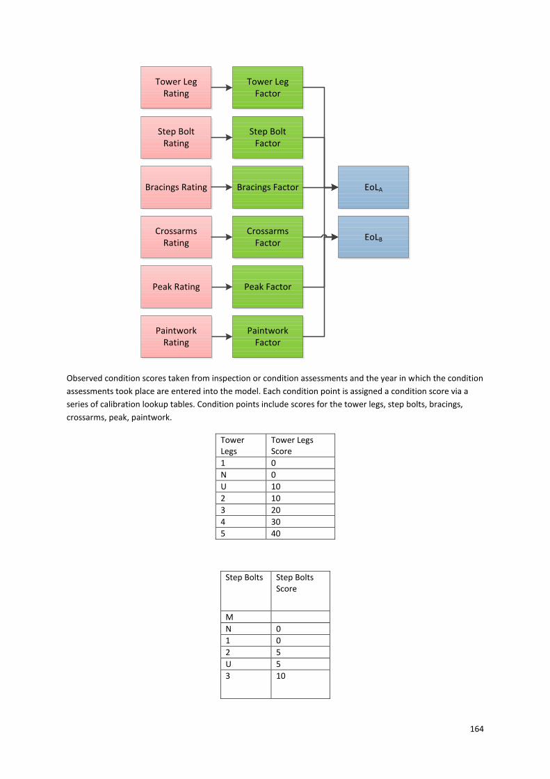
164

Observed condition scores taken from inspection or condition assessments and the year in which the condition

assessments took place are entered into the model. Each condition point is assigned a condition score via a

series of calibration lookup tables. Condition points include scores for the tower legs, step bolts, bracings,

crossarms, peak, paintwork.

Tower Legs

Tower Legs Score

1 0

N 0

U 10

2 10

3 20

4 30

5 40

Step Bolts Step Bolts Score

M

N 0

1 0

2 5

U 5

3 10

Tower Leg Rating

Step Bolt Rating

Bracings Rating

Crossarms Rating

Peak Rating

Paintwork Rating

Tower Leg Factor

Step Bolt Factor

Bracings Factor

Crossarms Factor

Peak Factor

Paintwork Factor

EoLA

EoLB

165

4 20

5 25

Bracings Bracings Score

1 0

N 0

U 10

2 10

3 20

4 30

5 40

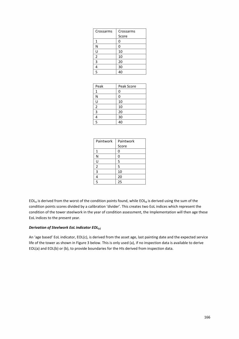
166

Crossarms Crossarms Score

1 0

N 0

U 10

2 10

3 20

4 30

5 40

Peak Peak Score

1 0

N 0

U 10

2 10

3 20

4 30

5 40

Paintwork Paintwork Score

1 0

N 0

U 5

2 5

3 10

4 20

5 25

EOLA is derived from the worst of the condition points found, while EOLB is derived using the sum of the

condition points scores divided by a calibration ‘divider’. This creates two EoL indices which represent the

condition of the tower steelwork in the year of condition assessment, the Implementation will then age these

EoL indices to the present year.

Derivation of Steelwork EoL indicator EOL(c)

An ‘age based’ EoL indicator, EOL(c), is derived from the asset age, last painting date and the expected service

life of the tower as shown in Figure 3 below. This is only used (a), if no inspection data is available to derive

EOL(a) and EOL(b) or (b), to provide boundaries for the HIs derived from inspection data.

167

Steelwork EoL indicator EOL(c)

The assets age is taken from the date of tower construction and where it exists, the date at which the tower

was last painted. If a tower has been painted then the expected life of the tower will be set via calibration to

an expected life associated with the paint system, typically in the region of 15 years. If the tower has not been

painted the year of construction is used against an expected life which is associated with the original tower

steelwork galvanising, a calibration value typically set at around 30 years.

Derivation of Steelwork EOL(y0)

The final tower steelwork EoL indicator, EOL(y0), which represents the present day overall condition of the

tower steelwork is determined from EOL(a), EOL(b) and EOL(c) as depicted below.

Tower Steelwork EOLS

Where detailed condition assessment information is not available, the model will not be able to calculate

EOL(a) or EOL(b), and therefore EOL(y0) will equal EOL(c).

Where detailed condition information is available the final tower steelwork EoL indicator, EOL(y0), will be the

maximum of EOL(a) and EOL(b). In the event that the condition assessment identifies that the tower steel work

in an as new condition, then the model will use EOL(c) to modify the EoL indicator depending upon the age of

the tower up to a calibratable limits which is typically set at a EOL of around 1.5.

Last Painting Date

Date of Construction

Age

Average Life

Location

Expected Life

EoLC

EoLS

EoLBEoLA EoLC

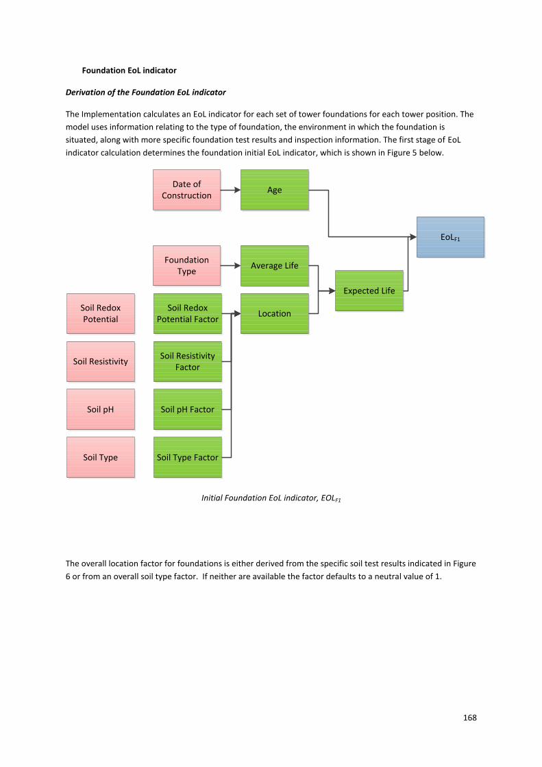
168

Foundation EoL indicator

Derivation of the Foundation EoL indicator

The Implementation calculates an EoL indicator for each set of tower foundations for each tower position. The

model uses information relating to the type of foundation, the environment in which the foundation is

situated, along with more specific foundation test results and inspection information. The first stage of EoL

indicator calculation determines the foundation initial EoL indicator, which is shown in Figure 5 below.

Initial Foundation EoL indicator, EOLF1

The overall location factor for foundations is either derived from the specific soil test results indicated in Figure

6 or from an overall soil type factor. If neither are available the factor defaults to a neutral value of 1.

Date of Construction

Age

Average Life

Location

Expected Life

EoLF1

Foundation Type

Soil Redox Potential Factor

Soil Resistivity Factor

Soil pH Factor

Soil Type Factor

Soil Redox Potential

Soil Type

Soil pH

Soil Resistivity

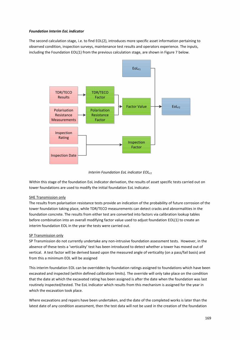
169

Foundation Interim EoL indicator


observed condition, inspection surveys, maintenance test results and operators experience. The inputs,

including the Foundation EOL(1) from the previous calculation stage, are shown in Figure 7 below.

Interim Foundation EoL indicator EOLF2

Within this stage of the foundation EoL indicator derivation, the results of asset specific tests carried out on

tower foundations are used to modify the initial foundation EoL indicator.

SHE Transmission only

The results from polarisation resistance tests provide an indication of the probability of future corrosion of the

tower foundation taking place, while TDR/TECO measurements can detect cracks and abnormalities in the

foundation concrete. The results from either test are converted into factors via calibration lookup tables

before combination into an overall modifying factor value used to adjust foundation EOL(1) to create an

interim foundation EOL in the year the tests were carried out.

SP Transmission only

SP Transmission do not currently undertake any non-intrusive foundation assessment tests. However, in the

absence of these tests a ‘verticality’ test has been introduced to detect whether a tower has moved out of

vertical. A test factor will be derived based upon the measured angle of verticality (on a pass/fail basis) and

from this a minimum EOL will be assigned

This interim foundation EOL can be overridden by foundation ratings assigned to foundations which have been

excavated and inspected (within defined calibration limits). The override will only take place on the condition

that the date at which the excavated rating has been assigned is after the date when the foundation was last

routinely inspected/tested. The EoL indicator which results from this mechanism is assigned for the year in

which the excavation took place.

Where excavations and repairs have been undertaken, and the date of the completed works is later than the

latest date of any condition assessment, then the test data will not be used in the creation of the foundation

Factor Value

EoLF1

TDR/TECO Factor

Polarisation Resistance

Factor

Inspection Factor

TDR/TECO Results

Inspection Date

Inspection Rating

Polarisation Resistance

Measurements

EoLF2

170

EoL indicator. Instead the EoL indicator will be based upon a calibration value which reflects the EoL of the

asset once the repairs have been completed (at the time of completion) and aged to the present year as

before.

1. Steel Tower EoL indicator

The Steel Tower EoL indicator is formed from the combination of the Tower Steelwork EoL indicator and the

Foundation Heath index, as shown in Figure 9 below.

Steel Tower EoL indicator

Once each of the input heath indices have been created, the Steel Tower EoL indicator is formed by taking a

weighted average of both the tower steelwork and the foundation EoL indices. This weighted average is

subject to a minimum EoL indicator override which is determined by calibration values. Traditionally the

weighting applied to the tower steelwork to foundation is in the region of 1:3, however this ratio can be

changed as part of a calibration review.

EoLT

EoLF2 EoLS

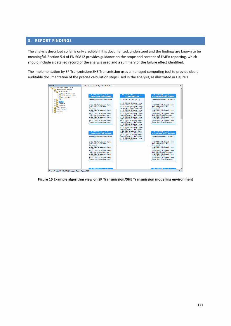
171

3. REPORT FINDINGS

The analysis described so far is only credible if it is documented, understood and the findings are known to be

meaningful. Section 5.4 of EN 60812 provides guidance on the scope and content of FMEA reporting, which

should include a detailed record of the analysis used and a summary of the failure effect identified.

The implementation by SP Transmission/SHE Transmission uses a managed computing tool to provide clear,

auditable documentation of the precise calculation steps used in the analysis, as illustrated in Figure 1.

Figure 15 Example algorithm view on SP Transmission/SHE Transmission modelling environment

Documents

Network Output Measures Methodology · 2017-03-14 · methodology for Network Output Measures (the NOMs methodology _) that: a. Facilitates the achievement of the NOMs methodology