Embed Size (px)
DESCRIPTION
Network Utility Maximization over Partially Observable Markov Channels. Channel State 1 = ?. 1. Channel State 2 = ?. 2. Channel State 3 = ?. 3. Restless Multi-Arm Bandit. Chih -Ping Li , Michael J. Neely University of Southern California - PowerPoint PPT Presentation
Citation preview
Network Utility Maximization over Partially Observable Markov Channels
Chih-Ping Li , Michael J. NeelyUniversity of Southern California
Information Theory and Applications Workshop, La Jolla, Feb. 2011
1 Channel State 1 = ?
Channel State 2 = ?
Channel State 3 = ?
2
3
Restless Multi-Arm Bandit

This work is from the following papers:*• Li, Neely WiOpt 2010 • Li, Neely ArXiv 2010, submitted for conference• Neely Asilomar 2010
Chih-Ping Li is graduating and is currently looking for post-doc positions!
*The above paper titles are given below, and are available at: http://www-bcf.usc.edu/~mjneely/• C. Li and M. J. Neely “Exploiting Channel Memory for Multi-User
Wireless Scheduling without Channel Measurement: Capacity Regions and Algorithms,” Proc. WiOpt 2010.
• C. Li and M. J. Neely, “Network Utility Maximization over Partially Observable Markovian Channels,” arXiv:1008.3421, Aug. 2010.
• M. J. Neely, “Dynamic Optimization and Learning for Renewal Systems,” Proc. Asilomar Conf. on Signals, Systems, and Computers, Nov. 2010.
1 S1(t) = ?
S2(t) = ?
S3(t) = ?2
3
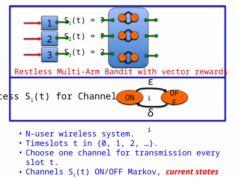
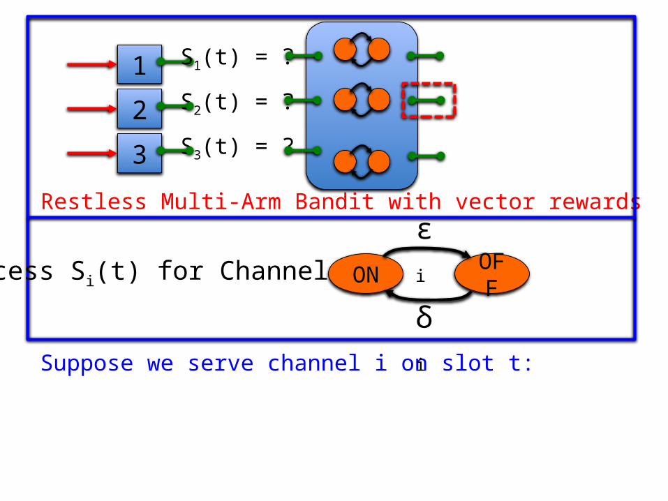
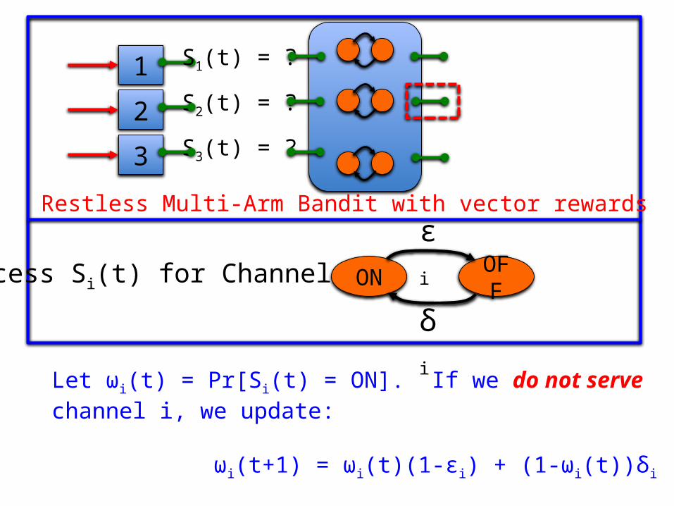
• N-user wireless system. • Timeslots t in {0, 1, 2, …}. • Choose one channel for transmission every slot t.• Channels Si(t) ON/OFF Markov, current states Si(t) unknown.
Process Si(t) for Channel i: ON OFF
εi
δi
Restless Multi-Arm Bandit with vector rewards
1 S1(t) = ?
S2(t) = ?
S3(t) = ?2
3
Restless Multi-Arm Bandit with vector rewards
Suppose we serve channel i on slot t:
Process Si(t) for Channel i: ON OFF
εi
δi
1 S1(t) = ?
S2(t) = ?
S3(t) = ?2
3
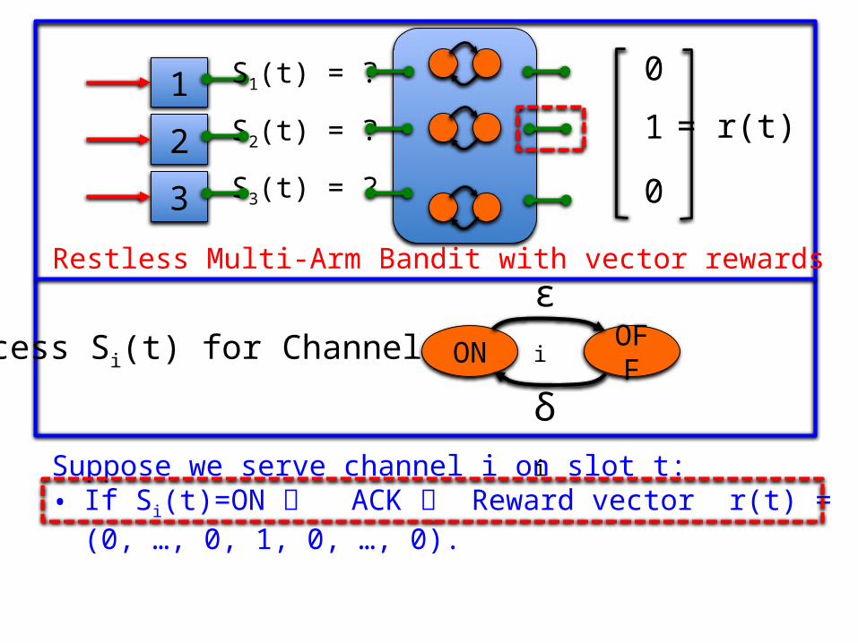
Suppose we serve channel i on slot t: • If Si(t)=ON ACK Reward vector r(t) = (0, …, 0, 1, 0, …, 0).
Process Si(t) for Channel i: ON OFF
εi
δi
0
1
0
Restless Multi-Arm Bandit with vector rewards
= r(t)
1 S1(t) = ?
S2(t) = ?
S3(t) = ?2
3
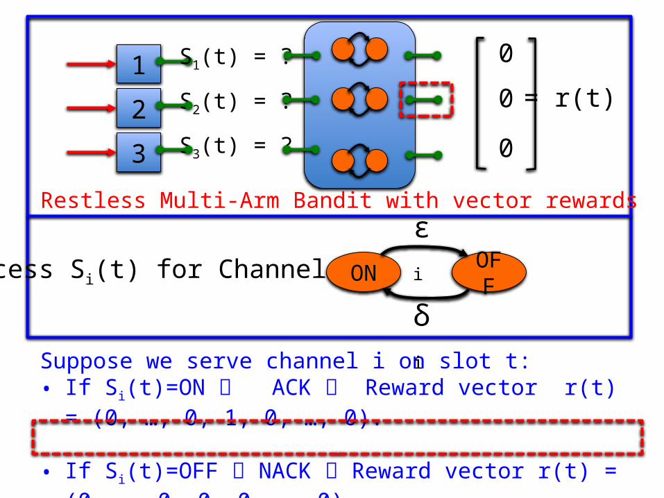
Suppose we serve channel i on slot t: • If Si(t)=ON ACK Reward vector r(t) = (0, …, 0, 1, 0, …, 0).
• If Si(t)=OFF NACK Reward vector r(t) = (0, …, 0, 0, 0, …, 0).
Process Si(t) for Channel i: ON OFF
εi
δi
0
0
0
= r(t)
Restless Multi-Arm Bandit with vector rewards
1 S1(t) = ?
S2(t) = ?
S3(t) = ?2
3
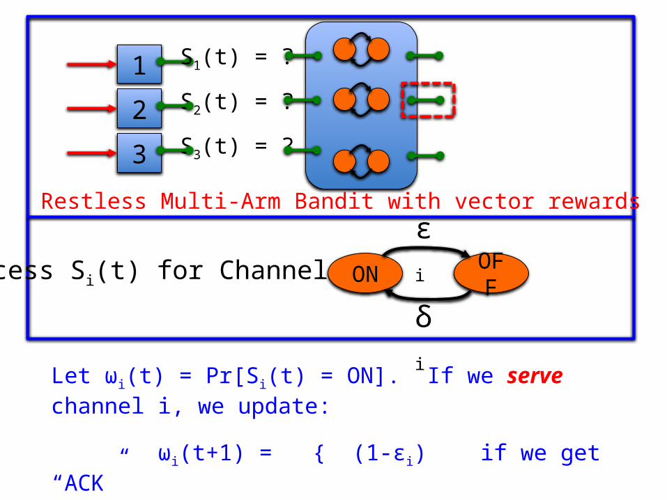
Let ωi(t) = Pr[Si(t) = ON]. If we serve channel i, we update:
ωi(t+1) = { (1-εi) if we get “ACK” { δi if we get “NACK”
Process Si(t) for Channel i: ON OFF
εi
δi
Restless Multi-Arm Bandit with vector rewards
1 S1(t) = ?
S2(t) = ?
S3(t) = ?2
3
Let ωi(t) = Pr[Si(t) = ON]. If we do not serve channel i, we update:
ωi(t+1) = ωi(t)(1-εi) + (1-ωi(t))δi
Process Si(t) for Channel i: ON OFF
εi
δi
Restless Multi-Arm Bandit with vector rewards
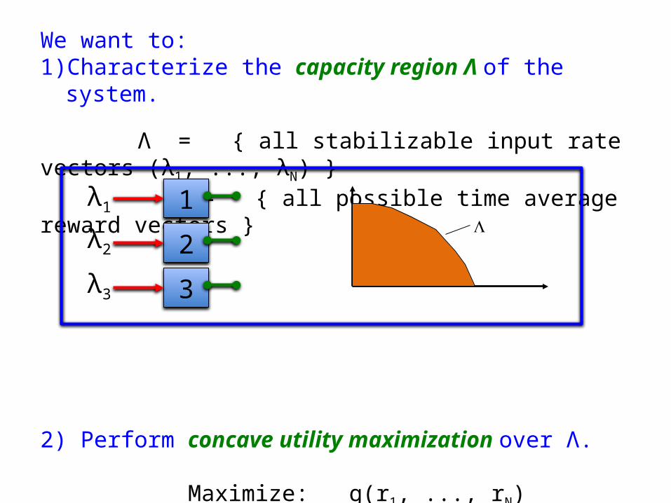
We want to: 1) Characterize the capacity region Λ of the system.
Λ = { all stabilizable input rate vectors (λ1, ..., λΝ) } = { all possible time average reward vectors }
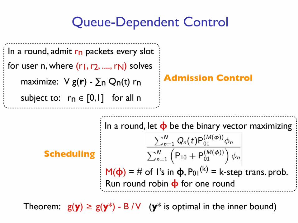
2) Perform concave utility maximization over Λ.
Maximize: g(r1, ..., rΝ)
Subject to: (r1, ..., rΝ) in Λ
1
2
3
λ1
λ2
λ3
L
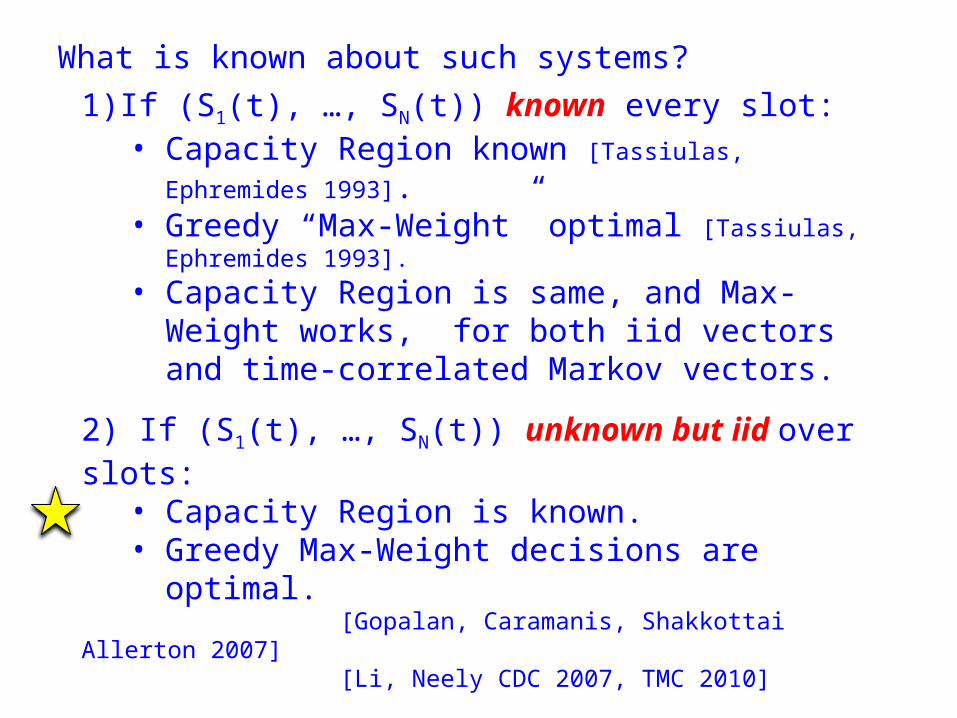
What is known about such systems? 1) If (S1(t), …, SN(t)) known every slot:• Capacity Region known [Tassiulas, Ephremides 1993].• Greedy “Max-Weight” optimal [Tassiulas, Ephremides 1993].• Capacity Region is same, and Max-Weight works, for
both iid vectors and time-correlated Markov vectors.
2) If (S1(t), …, SN(t)) unknown but iid over slots: • Capacity Region is known.• Greedy Max-Weight decisions are optimal.
[Gopalan, Caramanis, Shakkottai Allerton 2007] [Li, Neely CDC 2007, TMC 2010]
3) If (S1(t), …, SN(t)) unknown and time-correlated: • Capacity Region is unknown.• Seems to be an intractable multi-dimensional Markov
Decision Problem (MDP). Current decisions affect future (ω1(t), …, ωN(t)) probability vectors.
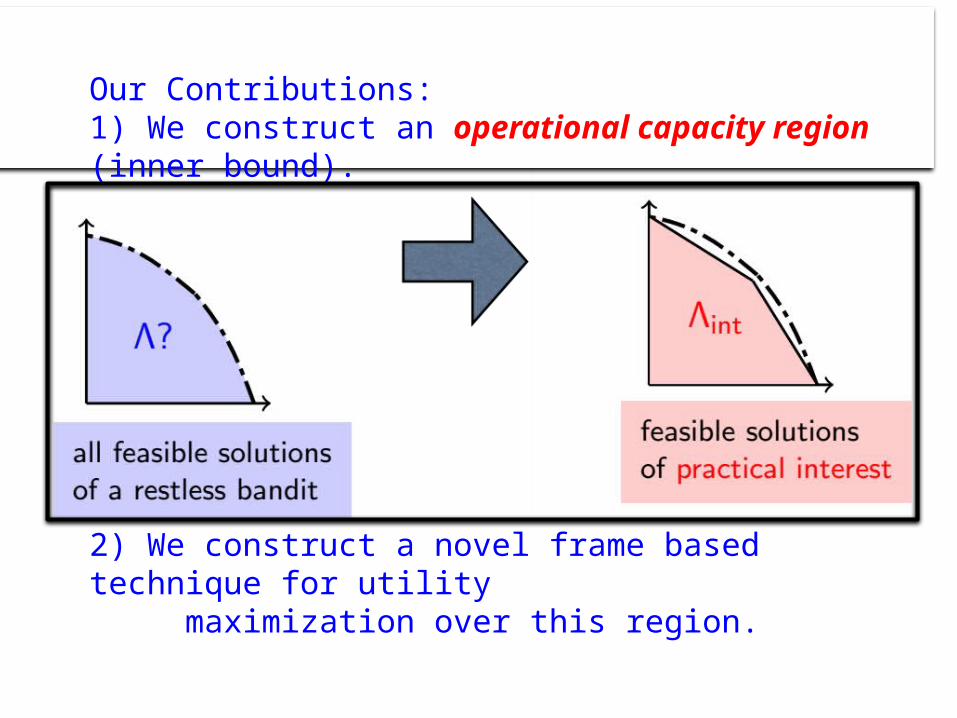
Our Contributions: 1) We construct an operational capacity region (inner bound).
Our Contributions: 1) We construct an operational capacity region (inner bound).
2) We construct a novel frame based technique for utility maximization over this region.
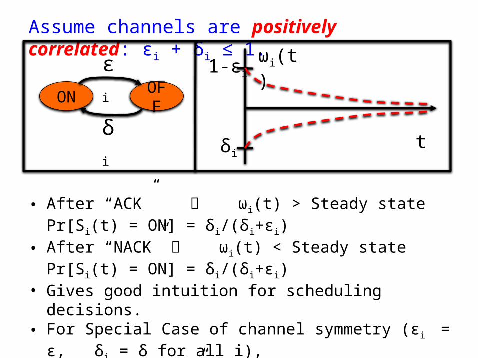
Assume channels are positively correlated: εi + δi ≤ 1.
ON OFF
εi
δi
ωi(t)
t
1-εi
δi
• After “ACK” ωi(t) > Steady state Pr[Si(t) = ON] = δi/(δi+εi)• After “NACK” ωi(t) < Steady state Pr[Si(t) = ON] = δi/(δi+εi)• Gives good intuition for scheduling decisions. • For Special Case of channel symmetry (εi = ε, δi = δ for all i), “round-robin” maximizes sum output rate. [Ahmad, Liu, Javidi, Zhao, Krishnamachari, Trans IT 2009]• How to use intuition to construct a capacity region (for possibly
asymmetric channels)?
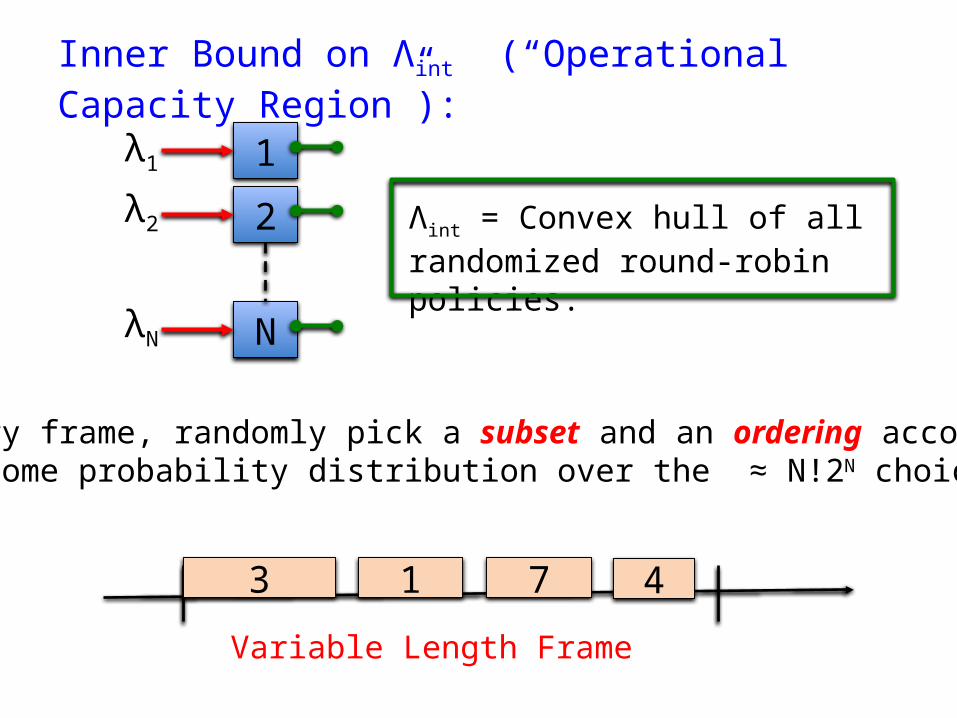
Inner Bound on Λint (“Operational Capacity Region”):
1
2
N
λ1
λ2
λN
3 1 7 4
Variable Length Frame
Every frame, randomly pick a subset and an ordering accordingto some probability distribution over the ≈ N!2N choices.
Λint = Convex hull of all randomized round-robin policies.
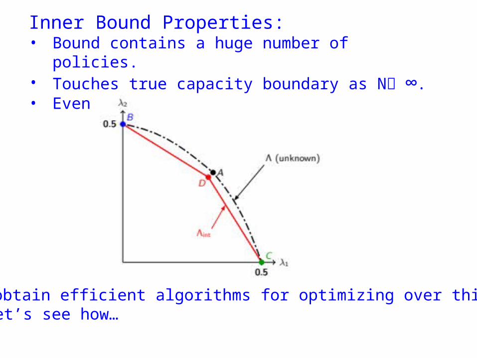
Inner Bound Properties:• Bound contains a huge number of policies.• Touches true capacity boundary as N ∞.• Even a good bound for N=2:
• Can obtain efficient algorithms for optimizing over this region! Let’s see how…
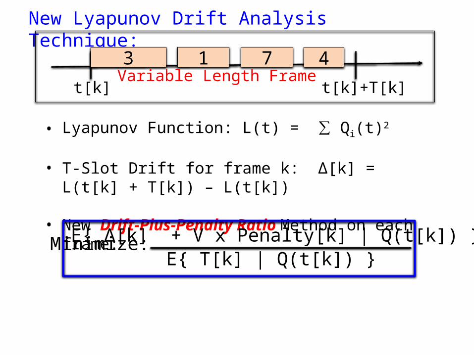
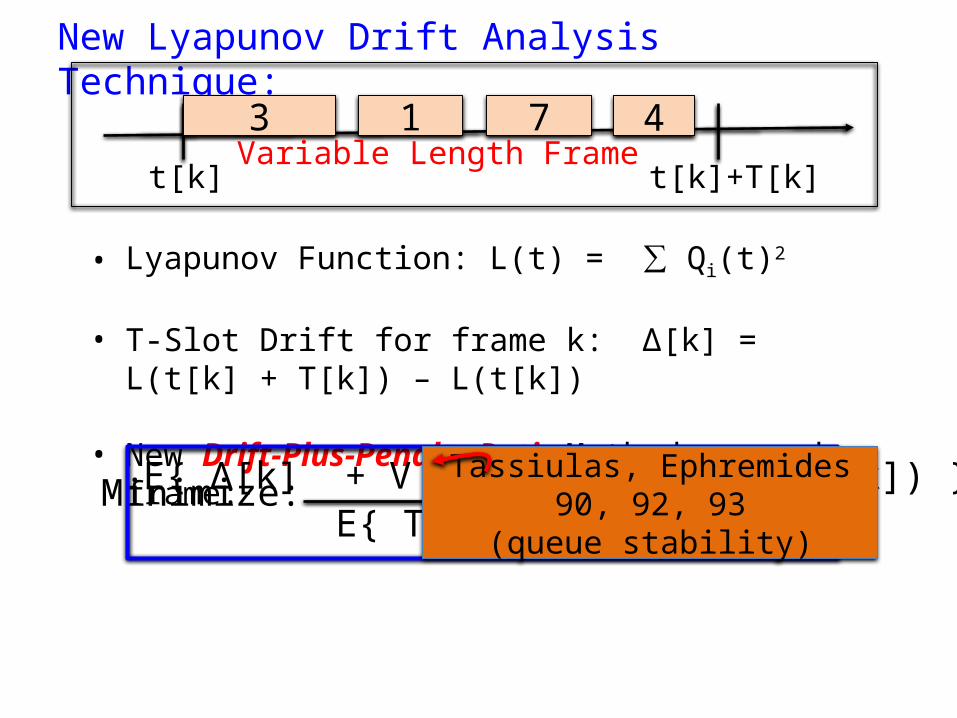
New Lyapunov Drift Analysis Technique:
• Lyapunov Function: L(t) = ∑ Qi(t)2
• T-Slot Drift for frame k: Δ[k] = L(t[k] + T[k]) – L(t[k])
• New Drift-Plus-Penalty Ratio Method on each frame:
3 1 7 4Variable Length Frame
t[k] t[k]+T[k]
Minimize: E{ Δ[k] + V x Penalty[k] | Q(t[k]) } E{ T[k] | Q(t[k]) }
New Lyapunov Drift Analysis Technique:
• Lyapunov Function: L(t) = ∑ Qi(t)2
• T-Slot Drift for frame k: Δ[k] = L(t[k] + T[k]) – L(t[k])
• New Drift-Plus-Penalty Ratio Method on each frame:
3 1 7 4Variable Length Frame
t[k] t[k]+T[k]
Minimize: E{ Δ[k] + V x Penalty[k] | Q(t[k]) } E{ T[k] | Q(t[k]) } Tassiulas, Ephremides 90, 92, 93
(queue stability)
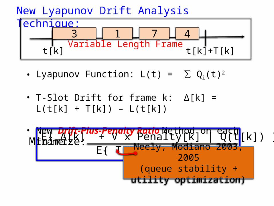
New Lyapunov Drift Analysis Technique:
• Lyapunov Function: L(t) = ∑ Qi(t)2
• T-Slot Drift for frame k: Δ[k] = L(t[k] + T[k]) – L(t[k])
• New Drift-Plus-Penalty Ratio Method on each frame:
3 1 7 4Variable Length Frame
t[k] t[k]+T[k]
Minimize: E{ Δ[k] + V x Penalty[k] | Q(t[k]) } E{ T[k] | Q(t[k]) } Neely, Modiano 2003, 2005
(queue stability + utility optimization)
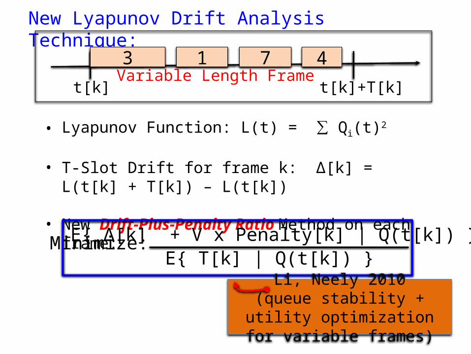
New Lyapunov Drift Analysis Technique:
• Lyapunov Function: L(t) = ∑ Qi(t)2
• T-Slot Drift for frame k: Δ[k] = L(t[k] + T[k]) – L(t[k])
• New Drift-Plus-Penalty Ratio Method on each frame:
3 1 7 4Variable Length Frame
t[k] t[k]+T[k]
Minimize: E{ Δ[k] + V x Penalty[k] | Q(t[k]) } E{ T[k] | Q(t[k]) }
Li, Neely 2010(queue stability + utility
optimization for variable frames)
Conclusions:
Quick Advertisement: New Book: M. J. Neely, Stochastic Network Optimization with Application to Communication and Queueing Systems. Morgan & Claypool, 2010.
• PDF also available from “Synthesis Lecture Series” (on digital library)• Link available on Mike Neely homepage. • Lyapunov Optimization theory (including renewal system problems)• Detailed Examples and Problem Set Questions.
• Multi-Armed Bandit Problem with Reward Vectors (complex MDP).
• Operational Capacity Region = Convex Hull over Frame-Based Randomized Round-Robin Policies.
• Stochastic Network Optimization via the Drift-Plus-Penalty Ratio method.