Embed Size (px)
Citation preview

Journal of Artificial Intelligence Research 33 (2008) 109-147 Submitted 11/07; published 9/08
Networks of Influence Diagrams: A Formalism forRepresenting Agents’ Beliefs and Decision-Making Processes
Ya’akov Gal [email protected] Computer Science and Artificial Intelligence LaboratoryHarvard School of Engineering and Applied Sciences
Avi Pfeffer [email protected]
Harvard School of Engineering and Applied Sciences
Abstract
This paper presents Networks of Influence Diagrams (NID), a compact, natural andhighly expressive language for reasoning about agents’ beliefs and decision-making pro-cesses. NIDs are graphical structures in which agents’ mental models are represented asnodes in a network; a mental model for an agent may itself use descriptions of the mentalmodels of other agents. NIDs are demonstrated by examples, showing how they can be usedto describe conflicting and cyclic belief structures, and certain forms of bounded rational-ity. In an opponent modeling domain, NIDs were able to outperform other computationalagents whose strategies were not known in advance. NIDs are equivalent in representationto Bayesian games but they are more compact and structured than this formalism. In par-ticular, the equilibrium definition for NIDs makes an explicit distinction between agents’optimal strategies, and how they actually behave in reality.
1. Introduction
In recent years, decision theory and game theory have had a profound impact on the designof intelligent systems. Decision theory provides a mathematical language for single-agentdecision-making under uncertainty, whereas game theory extends this language to the multi-agent case. On a fundamental level, both approaches provide a definition of what it meansto build an intelligent agent, by equating intelligence with utility maximization. Mean-while, graphical languages such as Bayesian networks (Pearl, 1988) have received muchattention in AI because they allow for a compact and natural representation of uncertaintyin many domains that exhibit structure. These formalisms often lead to significant savingsin representation and in inference time (Dechter, 1999; Cowell, Lauritzen, & Spiegelhater,2005).
Recently, a wide variety of representations and algorithms have augmented graphicallanguages to be able to represent and reason about agents’ decision-making processes. Forthe single-agent case, influence diagrams (Howard & Matheson, 1984) are able to representand to solve an agent’s decision making problem using the principles of decision theory.This representation has been extended to the multi-agent case, in which decision problemsare solved within a game-theoretic framework (Koller & Milch, 2001; Kearns, Littman, &Singh, 2001).
The focus in AI so far has been on the classical, normative approach to decision andgame theory. In the classical approach, a game specifies the actions that are available tothe agents, as well as their utilities that are associated with each possible set of agents’
c©2008 AI Access Foundation. All rights reserved.
Gal & Pfeffer
actions. The game is then analyzed to determine rational strategies for each of the agents.Fundamental to this approach are the assumptions that the structure of the game, includingagents’ utilities and their actions, is known to all of the agents, that agents’ beliefs aboutthe game are consistent with each other and correct, that all agents reason about the gamein the same way, and that all agents are rational in that they choose the strategy thatmaximizes their expected utility given their beliefs.
As systems involving multiple, autonomous agents become ubiquitous, they are increas-ingly deployed in open environments comprising human decision makers and computeragents that are designed by or represent different individuals or organizations. Examples ofsuch systems include on-line auctions, and patient care-delivery systems (MacKie-Mason,Osepayshivili, Reeves, & Wellman, 2004; Arunachalam & Sadeh, 2005). These settings arechallenging because no assumptions can be made about the decision-making strategies ofparticipants in open environments. Agents may be uncertain about the structure of thegame or about the beliefs of other agents about the structure of the game; they may useheuristics to make decisions or they may deviate from their optimal strategies (Camerer,2003; Gal & Pfeffer, 2003b; Rajarshi, Hanson, Kephart, & Tesauro, 2001).
To succeed in such environments, agents need to make a clear distinction between theirown decision-making models, the models others may be using to make decisions, and theextent to which agents deviate from these models when they actually make their decisions.This paper contributes a language, called Networks of Influence Diagrams (NID), that makesexplicit the different mental models agents may use to make their decisions. NIDs providefor a clear and compact representation with which to reason about agents’ beliefs andtheir decision-making processes. It allows multiple possible mental models of deliberationfor agents, with uncertainty over which models agents are using. It is recursive, so thatthe mental model for an agent may itself contain models of the mental models of otheragents, with associated uncertainty. In addition, NIDs allow agents’ beliefs to form cyclicstructures, of the form, “I believe that you believe that I believe,...”, and this cycle isexplicitly represented in the language. NIDs can also describe agents’ conflicting beliefsabout each other. For example, one can describe a scenario in which two agents disagreeabout the beliefs or behavior of a third agent.
NIDs are a graphical language whose building blocks are Multi Agent Influence Diagrams(MAID) (Koller & Milch, 2001). Each mental model in a NID is represented by a MAID,and the models are connected in a (possibly cyclic) graph. Any NID can be converted toan equivalent MAID that will represent the subjective beliefs of each agent in the game.
We provide an equilibrium definition for NIDs that combines the normative aspects ofdecision-making (what agents should do) with the descriptive aspects of decision-making(what agents are expected to do). The equilibrium makes an explicit distinction betweentwo types of strategies: Optimal strategies represent agents’ best course of action giventheir beliefs over others. Descriptive strategies represent how agents may deviate from theiroptimal strategy. In the classical approach to game theory, the normative aspect (whatagents should do) and the descriptive aspect (what analysts or other agents expect themto do), have coincided. Identification of these two aspects makes sense when an agent cando no better than optimize its decisions relative to its own model of the world. However,in open environments, it is important to consider the possibility that an agent is deviatingfrom its rational strategy with respect to its model.
110
Networks of Influence Diagrams
NIDs share a relationship with the Bayesian game formalism, commonly used to modeluncertainty over agents’ payoffs in economics (Harsanyi, 1967). In this formalism, thereis a type for each possible payoff function an agent may be using. Although NIDs arerepresentationally equivalent to Bayesian games, we argue that they are a more compact,succinct and natural representation. Any Bayesian game can be converted to a NID inlinear time. Any NID can be converted to a Bayesian game, but the size of the Bayesiangame may be exponential in the size of the NID.
This paper is a revised and expanded version of previous work (Gal & Pfeffer, 2003a,2003b, 2004), and is organized as follows: Section 2 presents the syntax of the NID language,and shows how they build on MAIDs in order to express the structure that holds betweenagents’ beliefs. Section 3 presents the semantics of NIDs in terms of MAIDs, and providesan equilibrium definition for NIDs. Section 4 provides a series of examples illustratingthe representational benefits of NIDs. It shows how agents can construct belief hierarchiesof each other’s decision-making in order to represent agents’ conflicting or incorrect beliefstructures, cyclic belief structures and opponent modeling. It also shows how certain formsof bounded rationality can be modeled by making a distinction between agents’ models ofdeliberation and the way they behave in reality. Section 5 demonstrates how NIDs can model“I believe that you believe” type reasoning in practice. It describes a NID that was ableto outperform the top programs that were submitted to a competition for automatic rock-paper-scissors players, whose strategy was not known in advance. Section 6 compares NIDsto several existing formalisms for describing uncertainty over decision-making processes. Itprovides a linear time algorithm for converting Bayesian games to NIDs. Finally, Section 7concludes and presents future work.
2. NID Syntax
The building blocks of NIDs are Bayesian networks (Pearl, 1988), and Multi Agent InfluenceDiagrams (Koller & Milch, 2001). A Bayesian network is a directed acyclic graph in whicheach node represents a random variable. An edge between two nodes X1 and X2 impliesthat X1 has a direct influence on the value of X2. Let Pa(Xi) represent the set of parentnodes for Xi in the network. Each node Xi contains a conditional probability distribution(CPD) over its domain for any value of its parents, denoted P (Xi | Pa(Xi)). The topologyof the network describes the conditional independence relationships that hold in the domain— every node in the network is conditionally independent of its non-descendants given itsparent nodes. A Bayesian network defines a complete joint probability distribution over itsrandom variables that can be decomposed as the product of the conditional probabilities ofeach node given its parent nodes. Formally,
P (X1, . . . , Xn) =n∏
i=1
P (Xi | Pa(Xi))
We illustrate Bayesian networks through the following example.
Example 2.1. Consider two baseball team managers Alice and Bob whose teams are play-ing the late innings of a game. Alice, whose team is hitting, can attempt to advance a runnerby instructing him to “steal” a base while the next pitch is being delivered. A successful
111
Gal & Pfeffer
steal will result in a benefit to the hitting team and a loss to the pitching team, or it mayresult in the runner being “thrown out”, incurring a large cost to the hitting team and abenefit to the pitching team. Bob, whose team is pitching, can instruct his team to throwa “pitch out”, thereby increasing the probability that a stealing runner will be thrown out.However, throwing a pitch out incurs a cost to the pitching team. The decisions whetherto steal and pitch out are taken simultaneously by both team managers. Suppose that thegame is not tied, that is either Alice’s or Bob’s team is leading in score, and that the identityof the leading team is known to Alice and Bob when they make their decision.
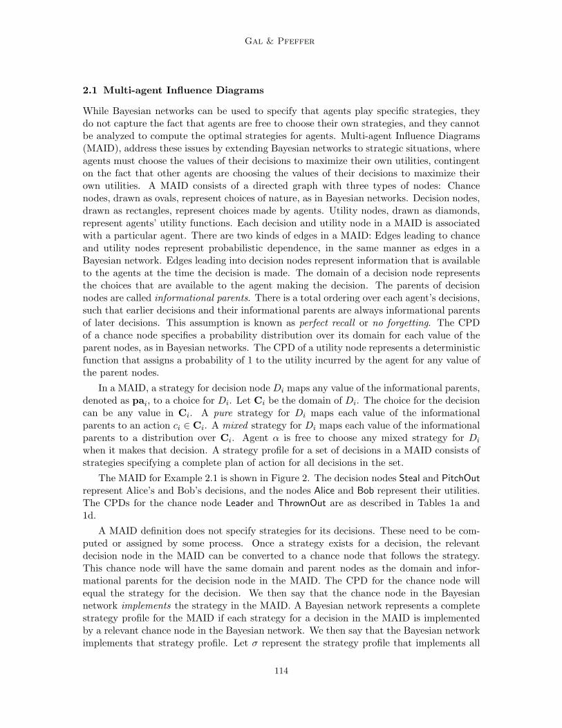
Suppose that Alice and Bob are using pre-specified strategies to make their decisionsdescribed as follows: when Alice is leading, she instructs a steal with probability 0.75,and Bob calls a pitch out with probability 0.90; when Alice is not leading, she instructsa steal with probability 0.65, and Bob calls a pitch out with probability 0.50. There aresix random variables in this domain: Steal and PitchOut represent the decisions for Aliceand Bob; ThrownOut represents whether the runner was thrown out; Leader represents theidentity of the leading team; Alice and Bob represent the utility functions for Alice and Bob.Figure 1 shows a Bayesian network for this scenario.
Steal PitchOut
ThrownOut
BobAlice
Leader
Figure 1: Bayesian network for Baseball Scenario (Example 2.1)
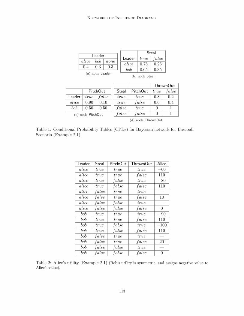
The CPD associated with each node in the network represents a probability distri-bution over its domain for any value of its parents. The CPDs for nodes Leader, Steal,PitchOut, and ThrownOut in this Bayesian network are shown in Table 1. For example, theCPD for ThrownOut, shown in Table 1d, represents the conditional probability distributionP (ThrownOut | Steal, PitchOut). According to the CPD, when Alice instructs a runner tosteal a base there is an 80% chance to get thrown out when Bob calls a pitch out and a 60%chance to get thrown out when Bob remains idle. The nodes Alice and Bob have determin-istic CPDs, assigning a utility for each agent for any joint value of the parent nodes Leader,Steal, PitchOut and ThrownOut. The utility for Alice is shown in Table 2. The utility forBob is symmetric and assigns the negative value assigned by Alice’s utility for the samevalue of the parent nodes. For example, when Alice is leading, and she instructs a runnerto steal a base, Bob instructs a pitch out, and the runner is thrown out, then Alice incursa utility of −60, while Bob incurs a utility of 60.1
1. Note that when Alice does not instruct to steal base, the runner cannot be thrown out, and the utilityfor both agents is not defined for this case.
112
Networks of Influence Diagrams
Leader
alice bob none
0.4 0.3 0.3(a) node Leader
Steal
Leader true false
alice 0.75 0.25bob 0.65 0.35
(b) node Steal
PitchOut
Leader true false
alice 0.90 0.10bob 0.50 0.50
(c) node PitchOut
ThrownOut
Steal PitchOut true false
true true 0.8 0.2true false 0.6 0.4false true 0 1false false 0 1
(d) node ThrownOut
Table 1: Conditional Probability Tables (CPDs) for Bayesian network for BaseballScenario (Example 2.1)
Leader Steal PitchOut ThrownOut Alice
alice true true true −60alice true true false 110alice true false true −80alice true false false 110alice false true true —alice false true false 10alice false false true —alice false false false 0bob true true true −90bob true true false 110bob true false true −100bob true false false 110bob false true true —bob false true false 20bob false false true —bob false false false 0
Table 2: Alice’s utility (Example 2.1) (Bob’s utility is symmetric, and assigns negative value toAlice’s value).
113
Gal & Pfeffer
2.1 Multi-agent Influence Diagrams
While Bayesian networks can be used to specify that agents play specific strategies, theydo not capture the fact that agents are free to choose their own strategies, and they cannotbe analyzed to compute the optimal strategies for agents. Multi-agent Influence Diagrams(MAID), address these issues by extending Bayesian networks to strategic situations, whereagents must choose the values of their decisions to maximize their own utilities, contingenton the fact that other agents are choosing the values of their decisions to maximize theirown utilities. A MAID consists of a directed graph with three types of nodes: Chancenodes, drawn as ovals, represent choices of nature, as in Bayesian networks. Decision nodes,drawn as rectangles, represent choices made by agents. Utility nodes, drawn as diamonds,represent agents’ utility functions. Each decision and utility node in a MAID is associatedwith a particular agent. There are two kinds of edges in a MAID: Edges leading to chanceand utility nodes represent probabilistic dependence, in the same manner as edges in aBayesian network. Edges leading into decision nodes represent information that is availableto the agents at the time the decision is made. The domain of a decision node representsthe choices that are available to the agent making the decision. The parents of decisionnodes are called informational parents. There is a total ordering over each agent’s decisions,such that earlier decisions and their informational parents are always informational parentsof later decisions. This assumption is known as perfect recall or no forgetting. The CPDof a chance node specifies a probability distribution over its domain for each value of theparent nodes, as in Bayesian networks. The CPD of a utility node represents a deterministicfunction that assigns a probability of 1 to the utility incurred by the agent for any value ofthe parent nodes.
In a MAID, a strategy for decision node Di maps any value of the informational parents,denoted as pai, to a choice for Di. Let Ci be the domain of Di. The choice for the decisioncan be any value in Ci. A pure strategy for Di maps each value of the informationalparents to an action ci ∈ Ci. A mixed strategy for Di maps each value of the informationalparents to a distribution over Ci. Agent α is free to choose any mixed strategy for Di
when it makes that decision. A strategy profile for a set of decisions in a MAID consists ofstrategies specifying a complete plan of action for all decisions in the set.
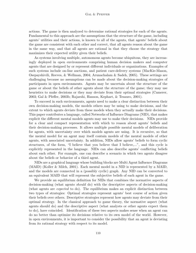
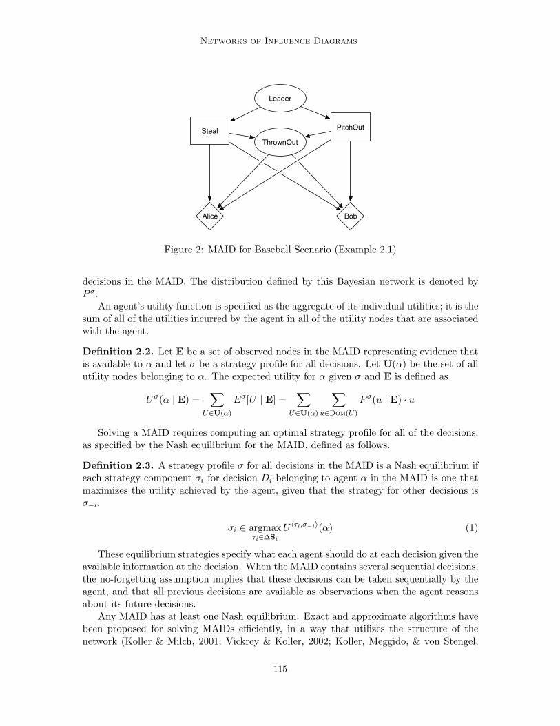
The MAID for Example 2.1 is shown in Figure 2. The decision nodes Steal and PitchOutrepresent Alice’s and Bob’s decisions, and the nodes Alice and Bob represent their utilities.The CPDs for the chance node Leader and ThrownOut are as described in Tables 1a and1d.
A MAID definition does not specify strategies for its decisions. These need to be com-puted or assigned by some process. Once a strategy exists for a decision, the relevantdecision node in the MAID can be converted to a chance node that follows the strategy.This chance node will have the same domain and parent nodes as the domain and infor-mational parents for the decision node in the MAID. The CPD for the chance node willequal the strategy for the decision. We then say that the chance node in the Bayesiannetwork implements the strategy in the MAID. A Bayesian network represents a completestrategy profile for the MAID if each strategy for a decision in the MAID is implementedby a relevant chance node in the Bayesian network. We then say that the Bayesian networkimplements that strategy profile. Let σ represent the strategy profile that implements all
114
Networks of Influence Diagrams
Steal PitchOut
ThrownOut
BobAlice
Leader
Figure 2: MAID for Baseball Scenario (Example 2.1)
decisions in the MAID. The distribution defined by this Bayesian network is denoted byP σ.
An agent’s utility function is specified as the aggregate of its individual utilities; it is thesum of all of the utilities incurred by the agent in all of the utility nodes that are associatedwith the agent.
Definition 2.2. Let E be a set of observed nodes in the MAID representing evidence thatis available to α and let σ be a strategy profile for all decisions. Let U(α) be the set of allutility nodes belonging to α. The expected utility for α given σ and E is defined as
Uσ(α | E) =∑
U∈U(α)
Eσ[U | E] =∑
U∈U(α)
∑u∈Dom(U)
P σ(u | E) · u
Solving a MAID requires computing an optimal strategy profile for all of the decisions,as specified by the Nash equilibrium for the MAID, defined as follows.
Definition 2.3. A strategy profile σ for all decisions in the MAID is a Nash equilibrium ifeach strategy component σi for decision Di belonging to agent α in the MAID is one thatmaximizes the utility achieved by the agent, given that the strategy for other decisions isσ−i.
σi ∈ argmaxτi∈ΔSi
U 〈τi,σ−i〉(α) (1)
These equilibrium strategies specify what each agent should do at each decision given theavailable information at the decision. When the MAID contains several sequential decisions,the no-forgetting assumption implies that these decisions can be taken sequentially by theagent, and that all previous decisions are available as observations when the agent reasonsabout its future decisions.
Any MAID has at least one Nash equilibrium. Exact and approximate algorithms havebeen proposed for solving MAIDs efficiently, in a way that utilizes the structure of thenetwork (Koller & Milch, 2001; Vickrey & Koller, 2002; Koller, Meggido, & von Stengel,
115
Gal & Pfeffer
1996; Blum, Shelton, & Koller, 2006). Exact algorithms for solving MAIDs decomposethe MAID graph into subsets of interrelated sub-games, and then proceed to find a set ofequilibria in these sub-games that together constitute a global equilibrium for the entiregame. In the case that there are multiple Nash equilibria, these algorithms will select oneof them, arbitrarily. The MAID in Figure 2 has a single Nash equilibrium, which we canobtain by solving the MAID: When Alice is leading, she instructs her runner to steal a basewith probability 0.2, and remain idle with probability 0.8, while Bob calls a pitch out withprobability 0.3, and remains idle with probability 0.7. When Bob is leading, Alice instructsa steal with probability 0.8, and Bob calls a pitch out with probability 0.5.
The Bayesian network that implements the Nash equilibrium strategy profile for theMAID can be queried to predict the likelihood of interesting events. For example, we canquery the network in Figure 2 and find that the probability that the stealer will get thrownout, given that agents’ strategies follow the Nash equilibrium strategy profile, is 0.57.
Any MAID can be converted to an extensive form game — a decision tree in whicheach vertex is associated with a particular agent or with nature. Splits in the tree representan assignment of values to chance and decision nodes in the MAID; leaves of the treerepresent the end of the decision-making process, and are labeled with the utilities incurredby the agents given the decisions and chance node values that are instantiated along theedges in the path leading to the leaf. Agents’ imperfect information regarding the actionsof others are represented by the set of vertices they cannot tell apart when they make aparticular decision. This set is referred to as an information set. Let D be a decision inthe MAID belonging to agent α. There is a one-to-one correspondence between values ofthe informational parents of D in the MAID and the information sets for α at the verticesrepresenting its move for decision D.
2.2 Networks of Influence Diagrams
To motivate NIDs, consider the following extension to Example 2.1.
Example 2.4. Suppose there are experts who will influence whether or not a team shouldsteal or pitch out. There is social pressure on the managers to follow the advice of theexperts, because if the managers’ decision turns out to be wrong they can assign blame tothe experts. The experts suggest that Alice should call a steal, and Bob should call a pitchout. This advice is common knowledge between the managers. Bob may be uncertain as towhether Alice will in fact follow the experts and steal, or whether she will ignore them andplay a best-response with respect to her beliefs about Bob. To quantify, Bob believes thatwith probability 0.7, Alice will follow the experts, while with probability 0.3, Alice will playbest-response. Alice’s beliefs about Bob are symmetric to Bob’s beliefs about Alice: Withprobability 0.7 Alice believes Bob will follow the experts and call a pitch out, and withprobability 0.3 Alice believes that Bob will play the best-response strategy with respectto his beliefs about Alice. The probability distribution for other variables in this exampleremains as shown in Table 1.
NIDs build on top of MAIDs to explicitly represent this structure. A Network of Influ-ence Diagrams (NID) is a directed, possibly cyclic graph, in which each node is a MAID.To avoid confusion with the internal nodes of each MAID, we will call the nodes of a NIDblocks. Let D be a decision belonging to agent α in block K, and let β be any agent. (In
116
Networks of Influence Diagrams
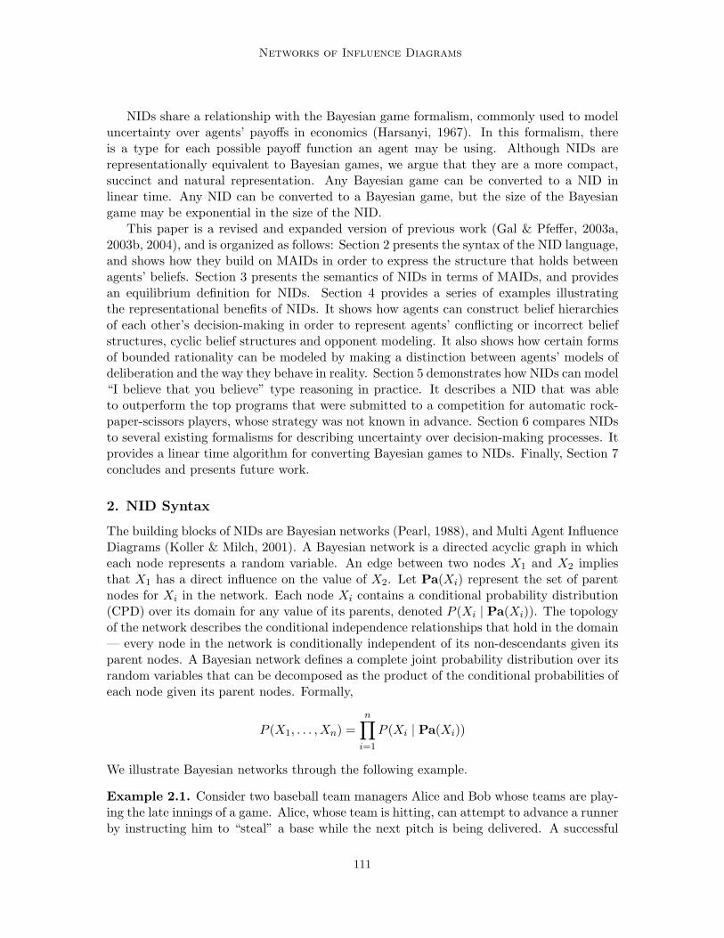
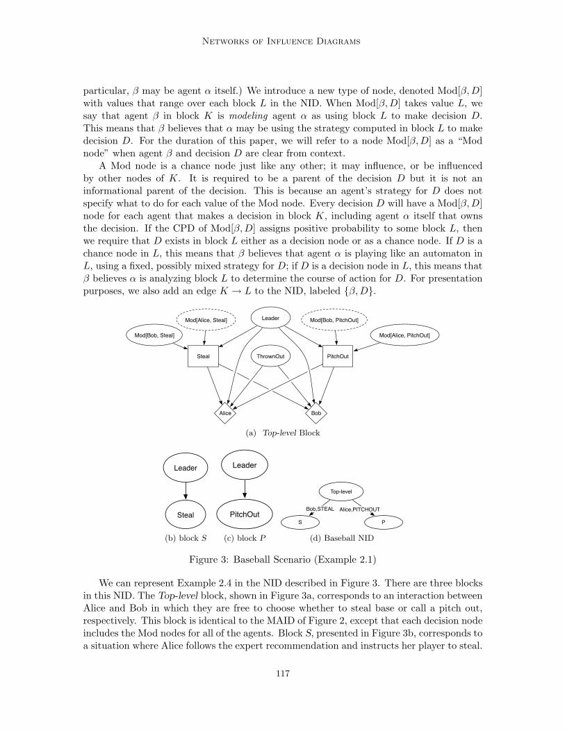
particular, β may be agent α itself.) We introduce a new type of node, denoted Mod[β, D]with values that range over each block L in the NID. When Mod[β, D] takes value L, wesay that agent β in block K is modeling agent α as using block L to make decision D.This means that β believes that α may be using the strategy computed in block L to makedecision D. For the duration of this paper, we will refer to a node Mod[β, D] as a “Modnode” when agent β and decision D are clear from context.
A Mod node is a chance node just like any other; it may influence, or be influencedby other nodes of K. It is required to be a parent of the decision D but it is not aninformational parent of the decision. This is because an agent’s strategy for D does notspecify what to do for each value of the Mod node. Every decision D will have a Mod[β, D]node for each agent that makes a decision in block K, including agent α itself that ownsthe decision. If the CPD of Mod[β, D] assigns positive probability to some block L, thenwe require that D exists in block L either as a decision node or as a chance node. If D is achance node in L, this means that β believes that agent α is playing like an automaton inL, using a fixed, possibly mixed strategy for D; if D is a decision node in L, this means thatβ believes α is analyzing block L to determine the course of action for D. For presentationpurposes, we also add an edge K → L to the NID, labeled {β, D}.
Steal PitchOutThrownOut
Mod[Bob, Steal] Mod[Alice, PitchOut]
BobAlice
Mod[Alice, Steal] Mod[Bob, PitchOut]Leader
(a) Top-level Block
Steal
Leader
(b) block S
PitchOut
Leader
(c) block P
Top-level
S P
Alice,PITCHOUTBob,STEAL
(d) Baseball NID
Figure 3: Baseball Scenario (Example 2.1)
We can represent Example 2.4 in the NID described in Figure 3. There are three blocksin this NID. The Top-level block, shown in Figure 3a, corresponds to an interaction betweenAlice and Bob in which they are free to choose whether to steal base or call a pitch out,respectively. This block is identical to the MAID of Figure 2, except that each decision nodeincludes the Mod nodes for all of the agents. Block S, presented in Figure 3b, corresponds toa situation where Alice follows the expert recommendation and instructs her player to steal.
117
Gal & Pfeffer
Mod[Bob, Steal]Top-level S
0.3 0.7(a) nodeMod[Bob, Steal]
Mod[Alice, PitchOut]Top-level P
0.3 0.7(b) nodeMod[Alice, PitchOut]
Mod[Bob, PitchOut]Top-level
1(c) nodeMod[Bob, PitchOut]
Mod[Alice, Steal]Top-level
1(d) nodeMod[Alice, Steal]
Table 3: CPDs for Top-level block of NID for Baseball Scenario (Example 2.1)
In this block, the Steal decision is replaced with a chance node, which assigns probability1 to true for any value of the informational parent Leader. Similarly, block P, presented inFigure 3c, corresponds to a situation where Bob instructs his team to pitch out. In thisblock, the PitchOut decision is replaced with a chance node, which assigns probability 1 totrue for any value of the informational parent Leader.
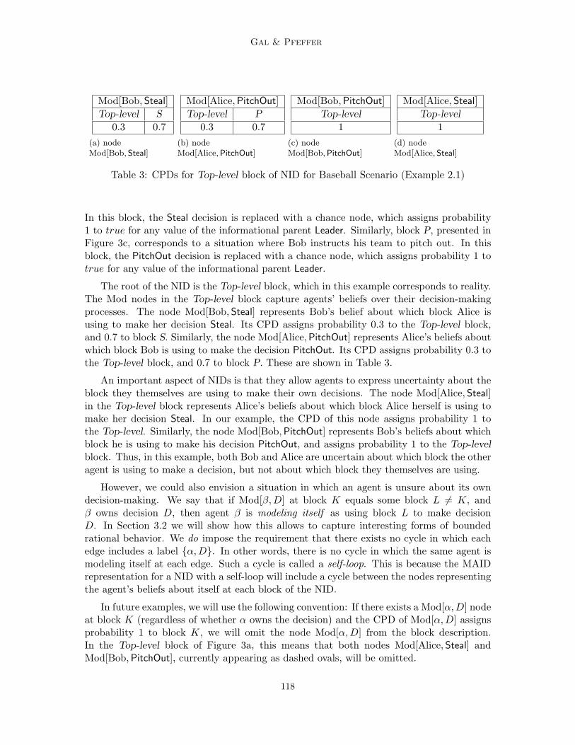
The root of the NID is the Top-level block, which in this example corresponds to reality.The Mod nodes in the Top-level block capture agents’ beliefs over their decision-makingprocesses. The node Mod[Bob, Steal] represents Bob’s belief about which block Alice isusing to make her decision Steal. Its CPD assigns probability 0.3 to the Top-level block,and 0.7 to block S. Similarly, the node Mod[Alice, PitchOut] represents Alice’s beliefs aboutwhich block Bob is using to make the decision PitchOut. Its CPD assigns probability 0.3 tothe Top-level block, and 0.7 to block P. These are shown in Table 3.
An important aspect of NIDs is that they allow agents to express uncertainty about theblock they themselves are using to make their own decisions. The node Mod[Alice, Steal]in the Top-level block represents Alice’s beliefs about which block Alice herself is using tomake her decision Steal. In our example, the CPD of this node assigns probability 1 tothe Top-level. Similarly, the node Mod[Bob, PitchOut] represents Bob’s beliefs about whichblock he is using to make his decision PitchOut, and assigns probability 1 to the Top-levelblock. Thus, in this example, both Bob and Alice are uncertain about which block the otheragent is using to make a decision, but not about which block they themselves are using.
However, we could also envision a situation in which an agent is unsure about its owndecision-making. We say that if Mod[β, D] at block K equals some block L �= K, andβ owns decision D, then agent β is modeling itself as using block L to make decisionD. In Section 3.2 we will show how this allows to capture interesting forms of boundedrational behavior. We do impose the requirement that there exists no cycle in which eachedge includes a label {α, D}. In other words, there is no cycle in which the same agent ismodeling itself at each edge. Such a cycle is called a self-loop. This is because the MAIDrepresentation for a NID with a self-loop will include a cycle between the nodes representingthe agent’s beliefs about itself at each block of the NID.
In future examples, we will use the following convention: If there exists a Mod[α, D] nodeat block K (regardless of whether α owns the decision) and the CPD of Mod[α, D] assignsprobability 1 to block K, we will omit the node Mod[α, D] from the block description.In the Top-level block of Figure 3a, this means that both nodes Mod[Alice, Steal] andMod[Bob, PitchOut], currently appearing as dashed ovals, will be omitted.
118
Networks of Influence Diagrams
3. NID Semantics
In this section we provide semantics for NIDs in terms of MAIDs. We first show how aNID can be converted to a MAID. We then define a NID equilibrium in terms of a Nashequilibrium of the constructed MAID.
3.1 Conversion to MAIDs
The following process converts each block K in the NID to a MAID fragment OK , and thenconnects them to form a MAID representation of the NID. The key construct in this processis the use of a chance node DK
α in the MAID to represent the beliefs of agent α regardingthe action that is chosen for decision D at block K. The value of Dα depends on the blockused by α to model decision D, as determined by the value of the Mod[α, D] node.
1. For each block K in the NID, we create a MAID OK . Any chance or utility node Nin block K that is a descendant of a decision node in K is replicated in OK , once foreach agent α, and denoted NK
α . If N is not a descendant of a decision node in K, itis copied to OK and denoted NK . In this case, we set NK
α = NK for any agent α.
2. If P is a parent of N in K, then PKα will be made a parent of NK
α in OK . The CPDof NK
α in OK will be equal to the CPD of N in K.
3. For each decision D in K, we create a decision node BR[D]K in OK , representing theoptimal action for α for this decision. If N is a chance or decision node which is aninformational parent of D in K, and D belongs to agent α, then NK
α will be made aninformational parent of BR[D]K in OK .
4. We create a chance node DKα in OK for each agent α. We make Mod[α, D]K a parent
of DKα . If decision D belongs to agent α, then we make BR[D]K a parent of DK
α . Ifdecision D belongs to agent β �= α, then we make DK
β a parent of DKα .
5. We assemble all the MAID fragments OK into a single MAID O as follows: We addan edge DL
α → DKβ where L �= K if L is assigned positive probability by Mod[β, D]K ,
and α owns decision D. Note that β may be any agent, including α itself.
6. We set the CPD of DKα to be a multiplexer. If α owns D then the CPD of DK
α assignsprobability 1 to BR[D]K when Mod[α, D]K equals K, and assigns probability 1 toDL
α when Mod[α, D]K equals L �= K. If β �= α owns D then the CPD of DKα assigns
probability 1 to DKβ when Mod[α, D]K equals K, and assigns probability 1 to DL
β
when Mod[α, D]K equals L �= K.
To explain, Step 1 of this process creates a MAID fragment OK for each NID block. Allnodes that are ancestors of decision nodes — representing events that occur prior to thedecisions — are copied to OK . However, events that occur after decisions are taken maydepend on the actions for those decisions. Every agent in the NID may have its own beliefsabout these actions and the events that follow them, regardless of whether that agent ownsthe decision. Therefore, all of the descendant nodes of decisions are duplicated for each agentin OK . Step 2 ensures that if any two nodes are connected in the original block K, then
119
Gal & Pfeffer
the nodes representing agents’ beliefs in OK are also connected. Step 3 creates a decisionnode in OK for each decision node in block K belonging to agent α. The informationalparents for the decision in OK are those nodes that represent the beliefs of α about itsinformational parents in K. Step 4 creates a separate chance node in OK for each agent αthat represents its belief about each of the decisions in K. If α owns the decision, this nodedepends on the decision node belonging to α. Otherwise, this node depends on the beliefsof α regarding the action of agent β that owns the decision. In the case that α models β asusing a different block to make the decisions, Step 5 connects between the MAID fragmentsof each block. Step 6 determines the CPDs for the nodes representing agents’ beliefs abouteach other’s decisions. The CPD ensures that the block that is used to model a decision isdetermined by the value of the Mod node. The MAID that is obtained as a result of thisprocess is a complete description of agents’ beliefs over each other’s decisions.
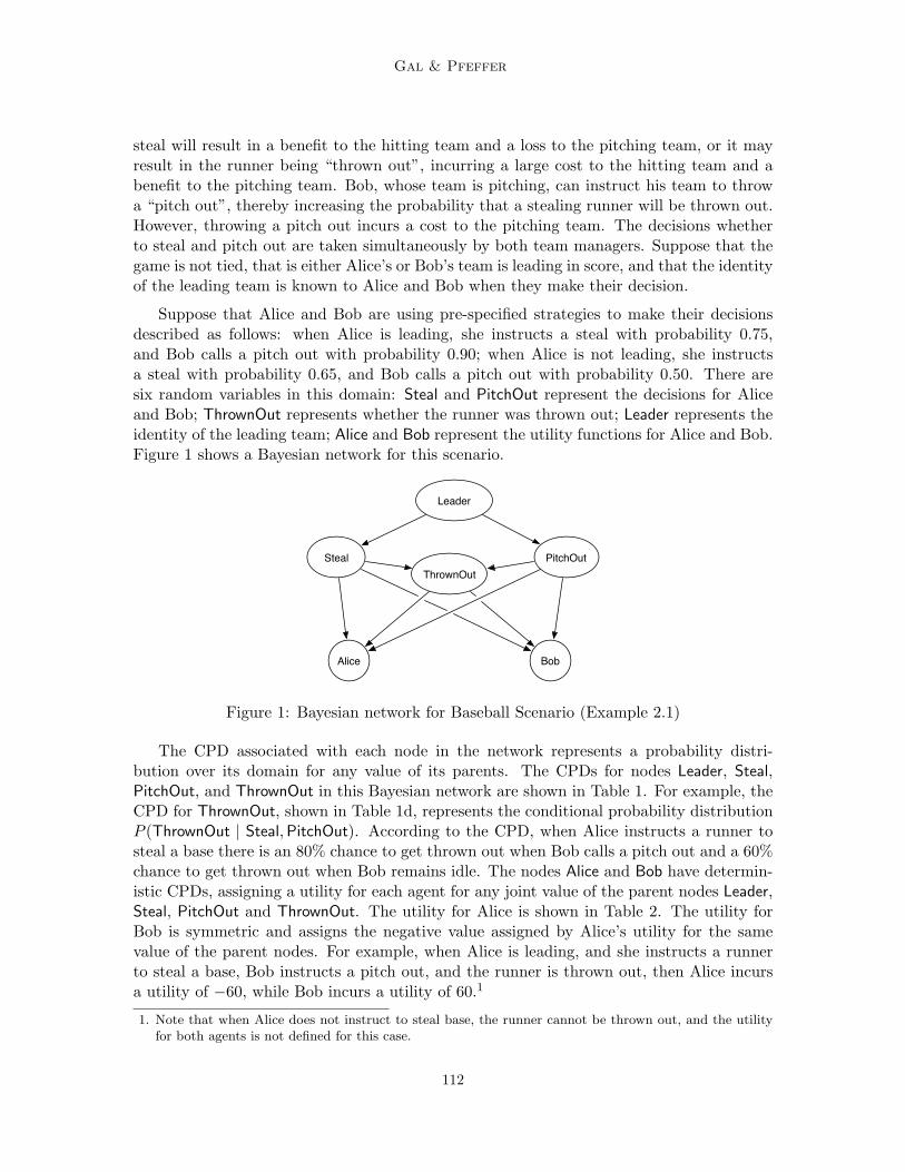
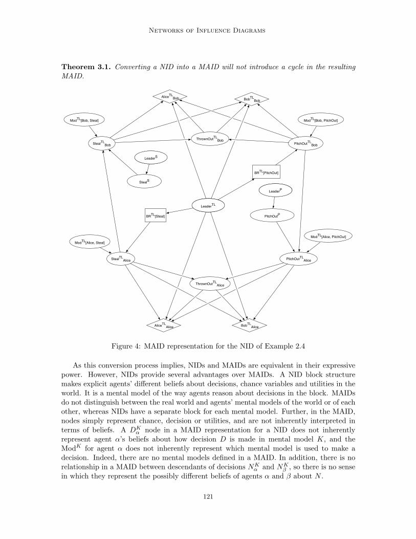
We demonstrate this process by converting the NID of Example 2.4 to its MAID repre-sentation, shown in Figure 4. First, MAID fragments for the three blocks Top-level, P, andS are created. The node Leader appearing in blocks Top-level, P, and S is not a descen-dant of any decision. Following Step 1, it is created once in each of the MAID fragments,giving the nodes LeaderTL, LeaderP and LeaderS . Similarly, the node Steal in block S andthe node PitchOut in block P are created once in each MAID fragment, giving the nodesStealS and PitchOutP . Also in Step 1, the nodes Mod[Alice, Steal]TL, Mod[Bob, Steal]TL,Mod[Alice, PitchOut]TL and Mod[Bob, PitchOut]TL are added to the MAID fragment for theTop-level block.
Step 3 adds the decision nodes BRTL[Steal] and BRTL[PitchOut] to the MAID fragmentfor the Top-level block. Step 4 adds the chance nodes PitchOutTL
Bob, PitchOutTLAlice, StealTL
Alice
and StealTLBob to the MAID fragment for the Top-level block. These nodes represent agents’
beliefs in this block about their own decisions or the decisions of other agents. For ex-ample, PitchOutTL
Bob represents Bob’s beliefs about its decision whether to pitch out, whilePitchOutTL
Alice represents Alice’s beliefs about Bob’s beliefs about this decision. Also follow-ing Step 4, edges BRTL[PitchOut] → PitchOutTL
Bob and StealTLAlice → StealTL
Bob are added to theMAID fragment for the Top-level block. These represent Bob’s beliefs over its own decisionat the block. An edge StealTL
Alice → StealTLBob is added to the MAID fragment to represent
Bob’s beliefs over Alice’s decision at the Top-level block. There are also nodes representingAlice’s beliefs about her and Bob’s decisions in this block.
In Step 5, edges StealS → StealTLBob and PitchOutP → PitchoutTL
Alice are added to theMAID fragment for the Top-level block. This is to allow Bob to reason about Alice’s decisionin block S, and for Alice to reason about Bob’s decision in block P. This action unifies theMAID fragments into a single MAID. The parents of StealTL
Bob are Mod[Bob, Steal]TL, StealS
and StealTLAlice. Its CPD is a multiplexer node that determines Bob’s prediction about Alice’s
action: If Mod[Bob, Steal]TL equals S, then Bob believes Alice to be using block S, in whichher action is to follow the experts and play strategy StealS . If Mod[Bob, Steal]TL equalsthe Top-level block, then Bob believes Alice to be using the Top-level block, in whichAlice’s action is to respond to her beliefs about Bob. The situation is similar for Alice’sdecision StealTL
Alice and the node Mod[Alice, Steal]TL with the following exception: WhenMod[Alice, Steal]TL equals the Top-level block, then Alice’s action follows her decision nodeBRTL[Steal].
In the Appendix, we prove the following theorem.
120
Networks of Influence Diagrams
Theorem 3.1. Converting a NID into a MAID will not introduce a cycle in the resultingMAID.
StealTLBob PitchOutTL
Bob
ModTL[Bob, Steal]
BobTLBob
AliceTLBob
ModTL[Bob, PitchOut]
ThrownOutTLBob
BRTL[PitchOut]
StealTLAlice PitchOutTL
Alice
ModTL[Alice, PitchOut]
BobTLAliceAliceTL
Alice
ModTL[Alice, Steal]
ThrownOutTLAlice
BRTL[Steal]
StealS
LeadBobLeaderTL
PitchOutP
LeadBobLeaderS
LeadBobLeaderP
Figure 4: MAID representation for the NID of Example 2.4
As this conversion process implies, NIDs and MAIDs are equivalent in their expressivepower. However, NIDs provide several advantages over MAIDs. A NID block structuremakes explicit agents’ different beliefs about decisions, chance variables and utilities in theworld. It is a mental model of the way agents reason about decisions in the block. MAIDsdo not distinguish between the real world and agents’ mental models of the world or of eachother, whereas NIDs have a separate block for each mental model. Further, in the MAID,nodes simply represent chance, decision or utilities, and are not inherently interpreted interms of beliefs. A DK
α node in a MAID representation for a NID does not inherentlyrepresent agent α’s beliefs about how decision D is made in mental model K, and theModK for agent α does not inherently represent which mental model is used to make adecision. Indeed, there are no mental models defined in a MAID. In addition, there is norelationship in a MAID between descendants of decisions NK
α and NKβ , so there is no sense
in which they represent the possibly different beliefs of agents α and β about N .
121
Gal & Pfeffer
Together with the NID construction process described above, a NID is a blueprintfor constructing a MAID that describes agents’ mental models. Without the NID, thisprocess becomes inherently difficult. Furthermore, the constructed MAID may be large andunwieldy compared to a NID block. Even for the simple NID of Example 2.4, the MAID ofFigure 4 is complicated and hard to understand.
3.2 Equilibrium Conditions
In Section 2.1, we defined pure and mixed strategies for decisions in MAIDs. In NIDs, weassociate the strategies for decisions with the blocks in which they appear. A pure strategyfor a decision D in a NID block K is a mapping from the informational parents of D toan action in the domain of D. Similarly, a mixed strategy for D is a mapping from theinformational parents of D to a distribution over the domain of D. A strategy profile for aNID is a set of strategies for all decisions at all blocks in the NID.
Traditionally, an equilibrium for a game is defined in terms of best response strategies.A Nash equilibrium is a strategy profile in which each agent is doing the best it possibly can,given the strategies of the other agents. Classical game theory predicts that all agents willplay a best response. NIDs, on the other hand, allow us to describe situations in which anagent deviates from its best response by playing according to some other decision-makingprocess. We would therefore like an equilibrium to specify not only what the agents shoulddo, but also to predict what they actually do, which may be different.
A NID equilibrium includes two types of strategies. The first, called a best responsestrategy, describes what the agents should do, given their beliefs about the decision-makingprocesses of other agents. The second, called an actually played strategy, describes whatagents will actually do according to the model described by the NID. These two strategiesare mutually dependent. The best response strategy for a decision in a block takes intoaccount the agent’s beliefs about the actually played strategies of all the other decisions.The actually played strategy for a decision in a block is a mixture of the best response forthe decision in the block, and the actually played strategies for the decision in other blocks.
Definition 3.2. Let N be a NID and let M be the MAID representation for N. Let σ be anequilibrium for M. Let D be a node belonging to agent α in block K of N. Let the parentsof D be Pa. By the construction of the MAID representation detailed in Section 3.1, theparents of BR[D]K in M are PaK
α and the domains of Pa and PaKα are the same. Let
σBR[D]K (pa) denote the mixed strategy assigned by σ for BR[D]K when PaKα equals pa.
The best response strategy for D in K, denoted θKD (pa), defines a function from values of
Pa to distributions over D that satisfy
θKD (pa) ≡ σBR[D]K (pa)
In other words, the best response strategy is the same as the MAID equilibrium whenthe corresponding parents take on the same values.
Definition 3.3. Let P σ denote the distribution that is defined by the Bayesian networkthat implements σ. The actually played strategy for decision D in K that is owned byagent α, denoted φK
D(pa), specifies a function from values of Pa to distributions over Dthat satisfy
φKD(pa) ≡ P σ(DK
α | pa)
122
Networks of Influence Diagrams
Note here, that DKα is conditioned on the informational parents of decision D rather than its
own parents. This node represents the beliefs of α about decision K. Therefore, the actuallyplayed strategy for D in K represents α’s belief about D in K, given the informationalparents of D.
Definition 3.4. Let σ be a MAID equilibrium. The NID equilibrium corresponding to σconsists of two strategy profiles θ and φ, such that for every decision D in every block K,θKD is the best response strategy for D in K, and φK
D is the actually played strategy for Din K.
For example, consider the constructed MAID for our baseball example in Figure 4. Thebest response strategies in the NID equilibrium specify strategies for the nodes Steal andPitchOut in the Top-level block that belong to Alice and Bob respectively. For an equi-librium σ of the MAID, the best response strategy for Steal in the Top-level block is thestrategy specified by σ for BRTL[Steal]. Similarily, the best response strategy for Pitchoutin the Top-level block is the strategy specified by σ for BRTL[Pitchout]. The actually playedstrategy for Steal in the Top-level is equal to the conditional probability distribution overStealTL
Alice given the informational parent LeaderTL. Similarly, the actually played strategyfor Pitchout is equal to the conditional probability distribution over PitchoutTL
Bob given theinformational parent LeaderTL. Solving this MAID yields the following unique equilibrium:In the NID Top-level block, the CPD for nodes Mod[Alice, Steal] and Mod[Bob, Pitchout]assigns probability 1 to the Top-level block, so the actually played and best response strate-gies for Bob and Alice are equal and specified as follows: If Alice is leading, then Alice stealsbase with probability 0.56 and Bob pitches out with probability 0.47. If Bob is leading,then Alice never steals base and Bob never pitches out. It turns out that because the ex-perts may instruct Bob to call a pitch out, Alice is considerably less likely to steal base,as compared to her equilibrium strategy for the MAID of Example 2.1, where none of themanagers considered the possibility that the other was being advised by experts. The caseis similar for Bob.
A natural consequence of this definition is that the problem of computing NID equilibriareduces to that of computing MAID equilibria. Solving the NID requires to convert it to itsMAID representation and solving the MAID using exact or approximate solution algorithms.The size of the MAID is bounded by the size of a block times the number of blocks timesthe number of agents. The structure of the NID can then be exploited by a MAID solutionalgorithm (Koller & Milch, 2001; Vickrey & Koller, 2002; Koller et al., 1996; Blum et al.,2006).
4. Examples
In this section, we provide a series of examples demonstrating the benefits of NIDs fordescribing and representing uncertainty over decision-making processes in a wide variety ofdomains.
4.1 Irrational Agents
Since the challenge to the notion of perfect rationality as the foundation of economic sys-tems presented by Simon (1955), the theory of bounded rationality has grown in different
123
Gal & Pfeffer
directions. From an economic point of view, bounded rationality dictates a complete de-viation from the utility maximizing paradigm, in which concepts such as “optimization”and “objective functions” are replaced with “satisficing” and “heuristics” (Gigerenzer &Selten, 2001). These concepts have recently been formalized by Rubinstein (1998). Froma traditional AI perspective, an agent exhibits bounded rationality if its program is a solu-tion to the constrained optimization problem brought about by limitations of architectureor computational resources (Russell & Wefald, 1991). NIDs serve to complement thesetwo prevailing perspectives by allowing to control the extent to which agents are behavingirrationally with respect to their model.
Irrationality is captured in our framework by the distinction between best response andactually played strategies. Rational agents always play a best response with respect totheir models. For rational agents, there is no distinction between the normative behaviorprescribed for each agent in each NID block, and the descriptive prediction of how the agentactually would play when using that block. In this case, the best response and actuallyplayed strategies of the agents are equal. However, in open systems, or when people areinvolved, we may need to model agents whose behavior differs from their best responsestrategy. In other words, their best response strategies and actually played strategies aredifferent. We can capture agent α behaving (partially) irrationally about its decision Dα
in block K by setting the CPD of Mod[α, Dα] to assign positive probability to some blockL �= K.
There is a natural way to express this distinction in NIDs through the use of the Modnode. If Dα is a decision associated with agent α, we can use Mod[α, Dα] to describe whichblock α actually uses to make the decision Dα. In block K, if Mod[α, Dα] is equal to K withprobability 1, then it means that within K, α is making the decision according to its beliefsin block K, meaning that α will be rational; it will play a best response to the strategiesof other agents, given its beliefs. If, however, Mod[α, Dα] assigns positive probability tosome block L other than K, it means that there is some probability that α will not playa best response to its beliefs in K, but rather play a strategy according to some otherblock L. In this case, we say α self-models at block K. The introduction of actually playedstrategies into the equilibrium definition represents another advantage of NIDs over MAIDs,in that they explicitly represent strategies for agents that may deviate from their optimalstrategies.
In some cases, making a decision may lead an agent to behave irrationally by viewingthe future in a considerably more positive light than is objectively likely. For example, aperson undergoing treatment for a disease may believe that the treatment stands a betterchance of success than scientifically plausible. In the psychological literature, this effectis referred to as motivational bias or positive illusion (Bazerman, 2001). As the followingexample shows, NIDs can represent agents’ motivational biases in a compelling way, bymaking Mod nodes depend on the outcome of decision nodes.
Example 4.1. Consider the case of a toothpaste company whose executives are facedwith two sequential decisions: whether to place an advertisement in a magazine for theirleading brand, and whether to increase production of the brand. Based on past analysis,the executives know that without advertising, the probability of high sales for the brand inthe next quarter will be 0.5. Placing the advertisement costs money, but the probabilityof high sales will rise to 0.7. Increasing production of the brand will contribute to profit
124
Networks of Influence Diagrams
if sales are high, but will hurt profit if sales are low due to the high cost of storage space.Suppose now that the company executives wish to consider the possibility of motivationalbias, in which placing the advertisement will inflate their beliefs about sales to be high inthe next quarter to probability 0.9. This may lead the company to increase the productionof the brand when it is not warranted by the market and consequently, suffer losses. Thecompany executives wish to compute their best possible strategy for their two decisionsgiven the fact that they attribute a motivational bias.
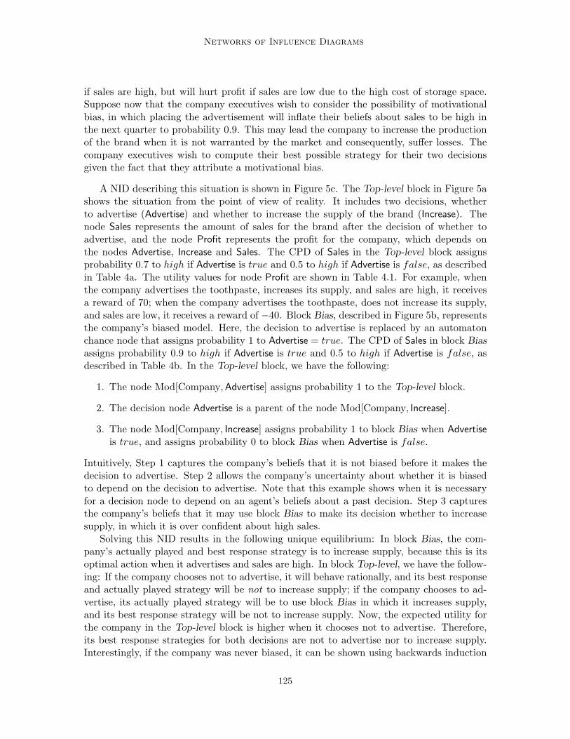
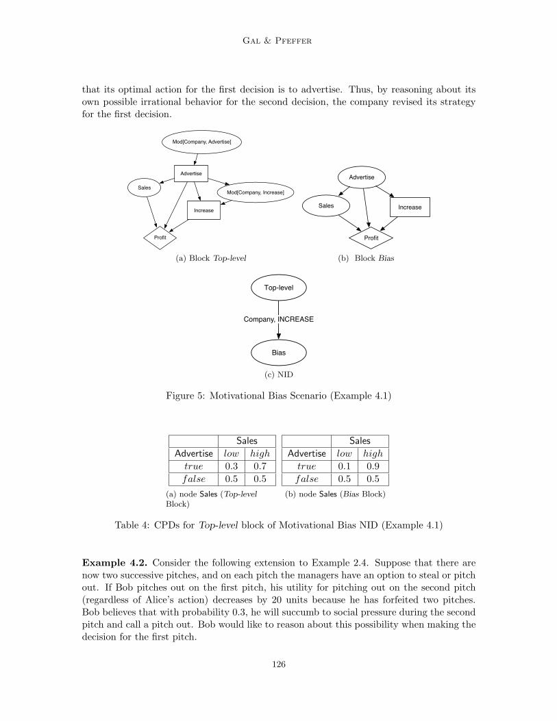
A NID describing this situation is shown in Figure 5c. The Top-level block in Figure 5ashows the situation from the point of view of reality. It includes two decisions, whetherto advertise (Advertise) and whether to increase the supply of the brand (Increase). Thenode Sales represents the amount of sales for the brand after the decision of whether toadvertise, and the node Profit represents the profit for the company, which depends onthe nodes Advertise, Increase and Sales. The CPD of Sales in the Top-level block assignsprobability 0.7 to high if Advertise is true and 0.5 to high if Advertise is false, as describedin Table 4a. The utility values for node Profit are shown in Table 4.1. For example, whenthe company advertises the toothpaste, increases its supply, and sales are high, it receivesa reward of 70; when the company advertises the toothpaste, does not increase its supply,and sales are low, it receives a reward of −40. Block Bias, described in Figure 5b, representsthe company’s biased model. Here, the decision to advertise is replaced by an automatonchance node that assigns probability 1 to Advertise = true. The CPD of Sales in block Biasassigns probability 0.9 to high if Advertise is true and 0.5 to high if Advertise is false, asdescribed in Table 4b. In the Top-level block, we have the following:
1. The node Mod[Company, Advertise] assigns probability 1 to the Top-level block.
2. The decision node Advertise is a parent of the node Mod[Company, Increase].
3. The node Mod[Company, Increase] assigns probability 1 to block Bias when Advertiseis true, and assigns probability 0 to block Bias when Advertise is false.
Intuitively, Step 1 captures the company’s beliefs that it is not biased before it makes thedecision to advertise. Step 2 allows the company’s uncertainty about whether it is biasedto depend on the decision to advertise. Note that this example shows when it is necessaryfor a decision node to depend on an agent’s beliefs about a past decision. Step 3 capturesthe company’s beliefs that it may use block Bias to make its decision whether to increasesupply, in which it is over confident about high sales.
Solving this NID results in the following unique equilibrium: In block Bias, the com-pany’s actually played and best response strategy is to increase supply, because this is itsoptimal action when it advertises and sales are high. In block Top-level, we have the follow-ing: If the company chooses not to advertise, it will behave rationally, and its best responseand actually played strategy will be not to increase supply; if the company chooses to ad-vertise, its actually played strategy will be to use block Bias in which it increases supply,and its best response strategy will be not to increase supply. Now, the expected utility forthe company in the Top-level block is higher when it chooses not to advertise. Therefore,its best response strategies for both decisions are not to advertise nor to increase supply.Interestingly, if the company was never biased, it can be shown using backwards induction
125
Gal & Pfeffer
that its optimal action for the first decision is to advertise. Thus, by reasoning about itsown possible irrational behavior for the second decision, the company revised its strategyfor the first decision.
Sales
Advertise
Increase
Profit
Mod[Company, Increase]
Mod[Company, Advertise]
(a) Block Top-level
Sales Increase
Profit
Advertise
(b) Block Bias
Top-level
Bias
Company, INCREASE
(c) NID
Figure 5: Motivational Bias Scenario (Example 4.1)
Sales
Advertise low high
true 0.3 0.7false 0.5 0.5
(a) node Sales (Top-levelBlock)
Sales
Advertise low high
true 0.1 0.9false 0.5 0.5
(b) node Sales (Bias Block)
Table 4: CPDs for Top-level block of Motivational Bias NID (Example 4.1)
Example 4.2. Consider the following extension to Example 2.4. Suppose that there arenow two successive pitches, and on each pitch the managers have an option to steal or pitchout. If Bob pitches out on the first pitch, his utility for pitching out on the second pitch(regardless of Alice’s action) decreases by 20 units because he has forfeited two pitches.Bob believes that with probability 0.3, he will succumb to social pressure during the secondpitch and call a pitch out. Bob would like to reason about this possibility when making thedecision for the first pitch.
126
Networks of Influence Diagrams
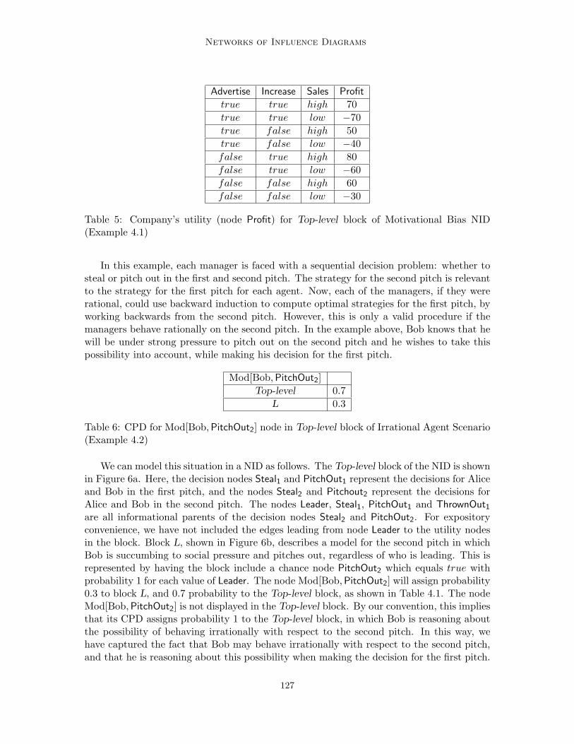
Advertise Increase Sales Profit
true true high 70true true low −70true false high 50true false low −40false true high 80false true low −60false false high 60false false low −30
Table 5: Company’s utility (node Profit) for Top-level block of Motivational Bias NID(Example 4.1)
In this example, each manager is faced with a sequential decision problem: whether tosteal or pitch out in the first and second pitch. The strategy for the second pitch is relevantto the strategy for the first pitch for each agent. Now, each of the managers, if they wererational, could use backward induction to compute optimal strategies for the first pitch, byworking backwards from the second pitch. However, this is only a valid procedure if themanagers behave rationally on the second pitch. In the example above, Bob knows that hewill be under strong pressure to pitch out on the second pitch and he wishes to take thispossibility into account, while making his decision for the first pitch.
Mod[Bob, PitchOut2]Top-level 0.7
L 0.3
Table 6: CPD for Mod[Bob, PitchOut2] node in Top-level block of Irrational Agent Scenario(Example 4.2)
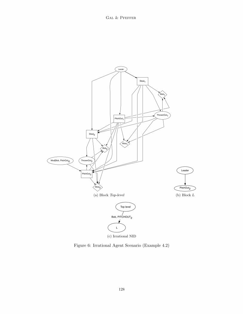
We can model this situation in a NID as follows. The Top-level block of the NID is shownin Figure 6a. Here, the decision nodes Steal1 and PitchOut1 represent the decisions for Aliceand Bob in the first pitch, and the nodes Steal2 and Pitchout2 represent the decisions forAlice and Bob in the second pitch. The nodes Leader, Steal1, PitchOut1 and ThrownOut1are all informational parents of the decision nodes Steal2 and PitchOut2. For expositoryconvenience, we have not included the edges leading from node Leader to the utility nodesin the block. Block L, shown in Figure 6b, describes a model for the second pitch in whichBob is succumbing to social pressure and pitches out, regardless of who is leading. This isrepresented by having the block include a chance node PitchOut2 which equals true withprobability 1 for each value of Leader. The node Mod[Bob, PitchOut2] will assign probability0.3 to block L, and 0.7 probability to the Top-level block, as shown in Table 4.1. The nodeMod[Bob, PitchOut2] is not displayed in the Top-level block. By our convention, this impliesthat its CPD assigns probability 1 to the Top-level block, in which Bob is reasoning aboutthe possibility of behaving irrationally with respect to the second pitch. In this way, wehave captured the fact that Bob may behave irrationally with respect to the second pitch,and that he is reasoning about this possibility when making the decision for the first pitch.
127
Gal & Pfeffer
Steal1
PitchOut1
ThrownOut1
Bob1
Alice1
Steal2
PitchOut2
ThrownOut2
Bob2
Alice2
Mod[Bob, PitchOut2]
Leader
(a) Block Top-level
PitchOut2
Leader
(b) Block L
Top level
L
Bob, PITCHOUT2
(c) Irrational NID
Figure 6: Irrational Agent Scenario (Example 4.2)
128
Networks of Influence Diagrams
There is a unique equilibrium for this NID. Both agents behave rationally for their firstdecision so their actually played and best response strategies are equal, and specified asfollows: Alice steals a base with probability 0.49 if she is leading, and never steals a baseif Bob is leading. Bob pitches out with probability 0.38 if Alice is leading and pitches outwith probability 0.51 if Bob is leading. In the second pitch, Alice behaves rationally, andher best response and actually played strategy are as follows: steal base with probability0.42 if Alice is leading and never steal base if Bob is leading. Bob may behave irrationallyin the second pitch: His best response strategy is to pitch out with probability 0.2 if Aliceis leading, and pitch out with probability 0.52 if Bob is leading; his actually played strategyis to pitch out with probability 0.58 if Alice is leading, and with probability 0.71 if Bob isleading. Note that because Bob is reasoning about his possible irrational behavior in thesecond pitch, he is less likely to pitch out in the first pitch as compared to the case in whichBob is completely rational (Example 2.4).
4.2 Conflicting Beliefs
In traditional game theory, agents’ beliefs are assumed to be consistent with a common priordistribution, meaning that the beliefs of agents about each other’s knowledge is expressedas a posterior probability distribution resulting from conditioning a common prior on eachagent’s information state. One consequence of this assumption is that agents’ beliefs candiffer only if they observe different information (Aumann & Brandenburger, 1995). Thisresult led to theoretic work that attempted to relax the common prior assumption. Myerson(1991) showed that a game with inconsistent belief structure that is finite can be convertedto a new game with consistent belief structures by constructing utility functions that areequivalent to the original game in a way that they both assign the same expected utilityto the agents. However, this new game will include beliefs and utility functions that arefundamentally different to the original game exhibiting the inconsistent belief structure. Fora summary of the economic and philosophical ramifications of relaxing the common priorassumption, see the work of Morris (1995) and Bonanno and Nehring (1999).
Once we have a language that allows us to talk about different mental models thatagents have about the world, and different beliefs that they have about each other andabout the structure of the game, it is natural to relax the common prior assumption withinNIDs while preserving the original structure of the game.
Example 4.3. Consider the following extension to the baseball scenario of Example 2.1.The probability that the runner is thrown out depends not only on the decisions of bothmanagers, but also on the speed of the runner. Suppose a fast runner will be thrown outwith 0.4 probability when Bob calls a pitch out, and with 0.2 probability when Bob doesnot call a pitch out. A slow runner will be thrown out with 0.8 probability when Bob callsa pitch out, and with 0.6 probability when Bob does not call a pitch out.
Now, Bob believes the runner to be slow, but is unsure about Alice’s beliefs regardingthe speed of the runner. With probability 0.8, Bob believes that Alice thinks that thestealer is fast, and with probability 0.2 Bob believes that Alice thinks that the stealer isslow. Assume that the distributions for other variables in this example are as described inTable 1.
129
Gal & Pfeffer
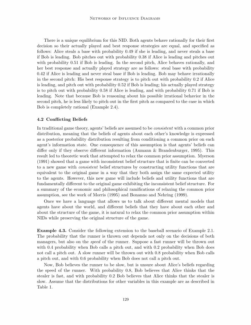
In this example, Bob is uncertain whether Alice’s beliefs about the speed of the runnerconflict with his own. NIDs allow to express this in a natural fashion by having two blocksthat describe the same decision-making process, but differ in the CPD that they assignto the speed of the runner. Through the use of the Mod node, NIDs can specify agents’conflicting beliefs about which of the two blocks is used by Alice to make her decision,according to Bob’s beliefs. The NID and blocks for this scenario are presented in Figure 7.
Speed
Steal PitchOutThrownOut
Mod[Bob, Steal]
BobAlice
Leader
(a) Top-level Block
Speed
Steal PitchOutThrownOut
BobAlice
Lead
(b) Block L
Top level
L
Bob,STEAL
(c) Conflicting Beliefs NID
Figure 7: Conflicting Beliefs Scenario (Example 4.3)
In the Top-level block, shown in Figure 7a, Bob and Alice decide whether to pitch out orto steal base, respectively. This block is identical in structure to the Top-level block of theprevious example, but it has an additional node Speed that is a parent of node ThrownOut,representing the fact that the speed of the runner affects the probability that the runner isthrown out.
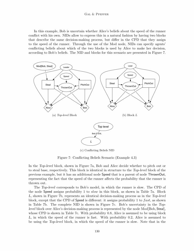
The Top-level corresponds to Bob’s model, in which the runner is slow. The CPD ofthe node Speed assigns probability 1 to slow in this block, as shown in Table 7a. BlockL, shown in Figure 7b, represents an identical decision-making process as in the Top-levelblock, except that the CPD of Speed is different: it assigns probability 1 to fast, as shownin Table 7b. The complete NID is shown in Figure 7c. Bob’s uncertainty in the Top-level block over Alice’s decision-making process is represented by the node Mod[Bob, Steal],whose CPD is shown in Table 7c. With probability 0.8, Alice is assumed to be using blockL, in which the speed of the runner is fast. With probability 0.2, Alice is assumed tobe using the Top-level block, in which the speed of the runner is slow. Note that in the
130
Networks of Influence Diagrams
Speed
fast slow
0 1(a) node Speed(block Top-level)
Speed
fast slow
1 0(b) node Speed(block L)
Mod[Bob, Steal]Top-level L
0.2 0.8(c) nodeMod[Bob, Steal] (blockTop-level)
Table 7: CPDs for nodes in Conflicting Beliefs NID (Example 4.3)
Top-level block, the nodes Mod[Alice, Steal], Mod[Alice, PitchOut] and Mod[Bob, PitchOut]are not displayed. By the convention introduced earlier, all these nodes assign probability1 to the Top-level block and have been omitted from the Top-level block of Figure 7a.Interestingly, this implies that Alice knows the runner to be slow, even though Bob believesthat Alice believes the runner is fast. When solving this NID, we get a unique equilibrium.Both agents are rational, so their best response and actually played strategies are equal,and specified as follows: In block L, the runner is fast, so Alice always steals base, and Bobalways calls a pitch out. In the Top-level block, Bob believes that Alice uses block L withhigh probability, in which she seals a base. In the Top-level block the speed of the runner isslow and will likely be thrown out. Therefore, Bob does not pitch out in order to maximizeits utility given its beliefs about Alice. In turn, Alice does not steal base at the Top-levelblock because the speed of the runner is slow at this block.
4.3 Collusion and Alliances
In a situation where an agent is modeling multiple agents, it may be important to knowwhether those agents are working together in some fashion. In such situations, the modelsof how the other agents make their decisions may be correlated, due to possible collusion.
Example 4.4. A voting game involves 3 agents Alice, Bob, and Carol, who are voting oneof them to be chairperson of a committee. Alice is the incumbent, and will be chairpersonif the vote ends in a draw. Each agent would like itself to be chairperson, and receivesutility 2 in that case. Alice also receives a utility of 1 if she votes for the winner but losesthe election, because she wants to look good. Bob and Carol, meanwhile, dislike Alice andreceive utility -1 if Alice wins.
It is in the best interests of agents Bob and Carol to coordinate, and both vote for thesame person. If Bob and Carol do indeed coordinate, it is in Alice’s best interest to vote forthe person they vote for. However, if Bob and Carol mis-coordinate, Alice should vote forherself to remain the chairperson. In taking an opponent modeling approach, Alice wouldlike to have a model of how Bob and Carol are likely to vote. Alice believes that withprobability 0.2, Bob and Carol do not collude; with probability 0.3, Bob and Carol colludeto vote for Bob; with probability 0.4, Bob and Carol collude to vote for Carol. Also, Alicebelieves that when they collude, both agents might renege and vote for themselves withprobability 0.1.
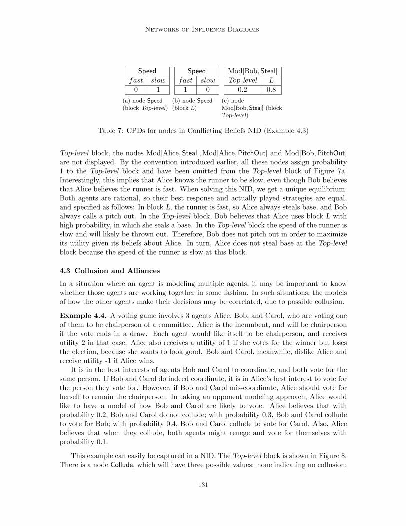
This example can easily be captured in a NID. The Top-level block is shown in Figure 8.There is a node Collude, which will have three possible values: none indicating no collusion;
131
Gal & Pfeffer
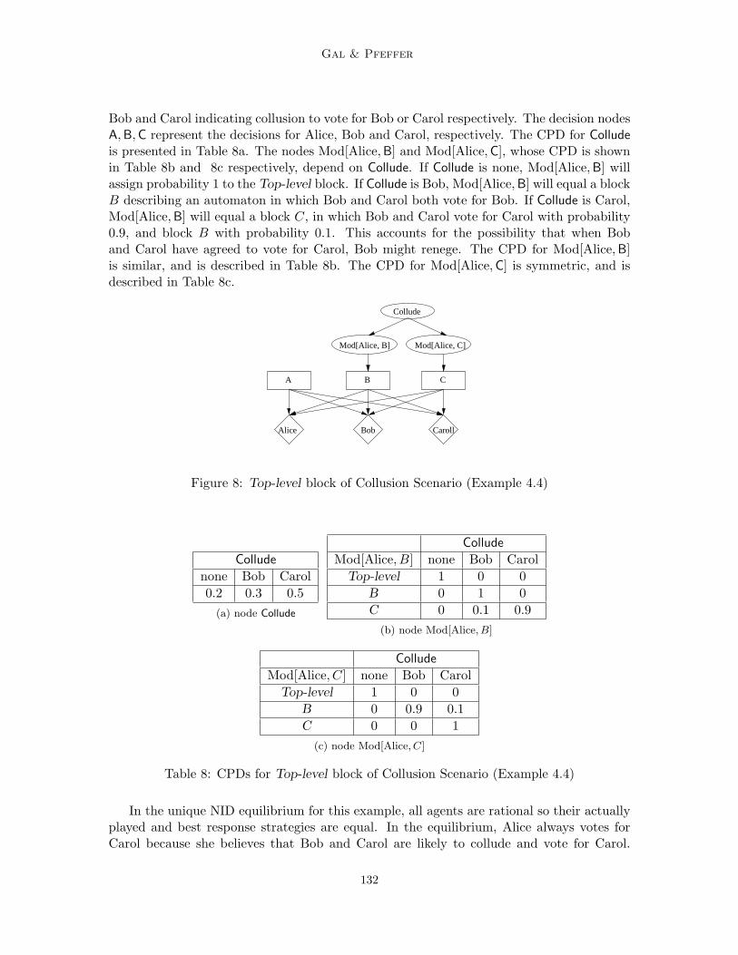
Bob and Carol indicating collusion to vote for Bob or Carol respectively. The decision nodesA, B, C represent the decisions for Alice, Bob and Carol, respectively. The CPD for Colludeis presented in Table 8a. The nodes Mod[Alice, B] and Mod[Alice, C], whose CPD is shownin Table 8b and 8c respectively, depend on Collude. If Collude is none, Mod[Alice, B] willassign probability 1 to the Top-level block. If Collude is Bob, Mod[Alice, B] will equal a blockB describing an automaton in which Bob and Carol both vote for Bob. If Collude is Carol,Mod[Alice, B] will equal a block C, in which Bob and Carol vote for Carol with probability0.9, and block B with probability 0.1. This accounts for the possibility that when Boband Carol have agreed to vote for Carol, Bob might renege. The CPD for Mod[Alice, B]is similar, and is described in Table 8b. The CPD for Mod[Alice, C] is symmetric, and isdescribed in Table 8c.
Caroll
A B C
Collude
Mod[Alice, B] Mod[Alice, C]
Alice Bob
Figure 8: Top-level block of Collusion Scenario (Example 4.4)
Collude
none Bob Carol0.2 0.3 0.5
(a) node Collude
Collude
Mod[Alice, B] none Bob CarolTop-level 1 0 0
B 0 1 0C 0 0.1 0.9
(b) node Mod[Alice, B]
Collude
Mod[Alice, C] none Bob CarolTop-level 1 0 0
B 0 0.9 0.1C 0 0 1
(c) node Mod[Alice, C]
Table 8: CPDs for Top-level block of Collusion Scenario (Example 4.4)
In the unique NID equilibrium for this example, all agents are rational so their actuallyplayed and best response strategies are equal. In the equilibrium, Alice always votes forCarol because she believes that Bob and Carol are likely to collude and vote for Carol.
132
Networks of Influence Diagrams
In turn, Carol votes for herslef or for Bob with probability 0.5, and Bob always votes forhimself. By reneging, Bob gives himself a chance to win the vote, in the case that Carolvotes for him.
Moving beyond this example, one of the most important issues in multi-player games isalliances. When players form an alliance, they will act for the benefit of the alliance ratherthan purely for their own self-interest. Thus an agent’s beliefs about the alliance structureaffects its models of how other agents make their decisions. When an agent has to make adecision in such a situation, it is important to be able to model its uncertainty about thealliance structure.
4.4 Cyclic Belief Structures
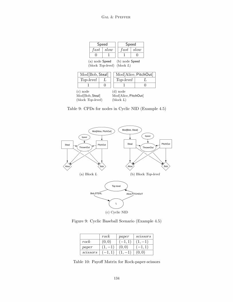
Cyclic belief structures are important in game theory, where they are used to model agentswho are symmetrically modeling each other. They are used to describe an infinite regress of“I think that you think that I think...” reasoning. Furthermore, cyclic belief structures canbe expressed in economic formalisms, like Bayesian games, so it is vital to allow them inNIDs in order for NIDs to encompass Bayesian games. Cyclic belief structures can naturallybe captured in NIDs by including a cycle in the NID graph.
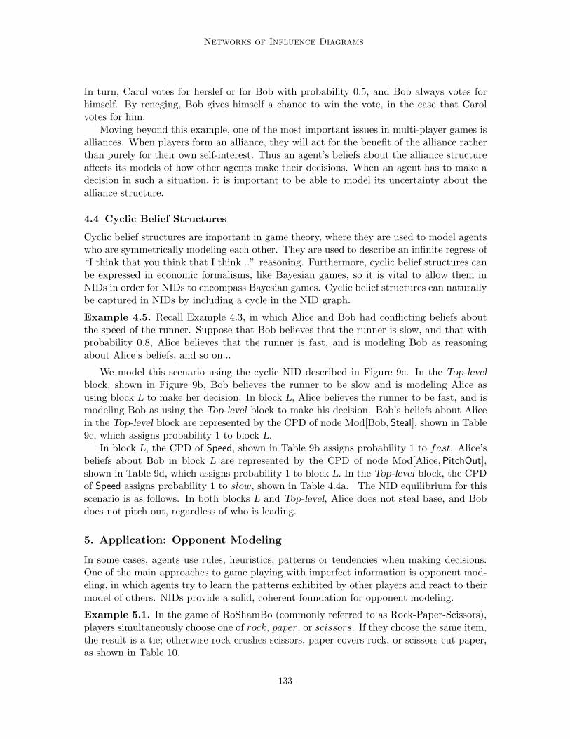
Example 4.5. Recall Example 4.3, in which Alice and Bob had conflicting beliefs aboutthe speed of the runner. Suppose that Bob believes that the runner is slow, and that withprobability 0.8, Alice believes that the runner is fast, and is modeling Bob as reasoningabout Alice’s beliefs, and so on...
We model this scenario using the cyclic NID described in Figure 9c. In the Top-levelblock, shown in Figure 9b, Bob believes the runner to be slow and is modeling Alice asusing block L to make her decision. In block L, Alice believes the runner to be fast, and ismodeling Bob as using the Top-level block to make his decision. Bob’s beliefs about Alicein the Top-level block are represented by the CPD of node Mod[Bob, Steal], shown in Table9c, which assigns probability 1 to block L.
In block L, the CPD of Speed, shown in Table 9b assigns probability 1 to fast. Alice’sbeliefs about Bob in block L are represented by the CPD of node Mod[Alice, PitchOut],shown in Table 9d, which assigns probability 1 to block L. In the Top-level block, the CPDof Speed assigns probability 1 to slow, shown in Table 4.4a. The NID equilibrium for thisscenario is as follows. In both blocks L and Top-level, Alice does not steal base, and Bobdoes not pitch out, regardless of who is leading.
5. Application: Opponent Modeling
In some cases, agents use rules, heuristics, patterns or tendencies when making decisions.One of the main approaches to game playing with imperfect information is opponent mod-eling, in which agents try to learn the patterns exhibited by other players and react to theirmodel of others. NIDs provide a solid, coherent foundation for opponent modeling.
Example 5.1. In the game of RoShamBo (commonly referred to as Rock-Paper-Scissors),players simultaneously choose one of rock, paper, or scissors. If they choose the same item,the result is a tie; otherwise rock crushes scissors, paper covers rock, or scissors cut paper,as shown in Table 10.
133
Gal & Pfeffer
Speed
fast slow
0 1(a) node Speed(block Top-level)
Speed
fast slow
1 0(b) node Speed(block L)
Mod[Bob, Steal]Top-level L
1 0(c) nodeMod[Bob, Steal](block Top-level)
Mod[Alice, PitchOut]Top-level L
1 0(d) nodeMod[Alice, PitchOut](block L)
Table 9: CPDs for nodes in Cyclic NID (Example 4.5)
Speed
Steal PitchOutThrownOut
Mod[Alice, PitchOut]
BobAlice
(a) Block L
Speed
Steal PitchOut
ThrownOut
Mod[Bob, Steal]
BobAlice
(b) Block Top-level
Top level
L
Bob,STEAL Alice,PITCHOUT
(c) Cyclic NID
Figure 9: Cyclic Baseball Scenario (Example 4.5)
rock paper scissors
rock (0, 0) (−1, 1) (1,−1)paper (1,−1) (0, 0) (−1, 1)scissors (−1, 1) (1,−1) (0, 0)
Table 10: Payoff Matrix for Rock-paper-scissors
134
Networks of Influence Diagrams
The game has a single Nash equilibrium in which both players play a mixed strategyover {rock, paper, scissors} with probability {1
3 , 13 , 1
3}. If both players do not deviate fromtheir equilibrium strategy, they are guaranteed an expected payoff of zero. In fact, it iseasy to verify that a player who always plays his equilibrium strategy is guaranteed toget an expected zero payoff regardless of the strategy of his opponent. In other words,sticking to the equilibrium strategy guarantees not to lose a match in expectation, but italso guarantees not to win it!
However, a player can try and win the game if the opponents are playing suboptimally.Any suboptimal strategy can be beaten, by predicting the next move of the opponent andthen employing a counter-strategy. The key to predicting the next move is to model thestrategy of the opponent, by identifying regularities in its past moves.
Now consider a situation in which two players play repeatedly against each other. Ifa player is able to pick up the tendencies of a suboptimal opponent, it might be able todefeat it, assuming the opponent continues to play suboptimally. In a recent competi-tion (Billings, 2000), programs competed against each other in matches consisting of 1000games of RoShamBo. As one might expect, Nash equilibrium players came in the middleof the pack because they broke even against every opponent. It turned out that the taskof modeling the opponent’s strategy can be surprisingly complex, despite the simple struc-ture of the game itself. This is because sophisticated players will attempt to counter-modeltheir opponents, and will hide their own strategy to avoid detection. The winning program,called Iocaine Powder (Egnor, 2000), did a beautiful job of modeling its opponents on mul-tiple levels. Iocaine Powder considered that its opponent might play randomly, accordingto some heuristic, or it might try to learn a pattern used by Iocaine Powder, or it mightplay a strategy designed to counter Iocaine Powder learning its pattern, or several otherpossibilities.
5.1 A NID for Modeling Belief Hierarchies
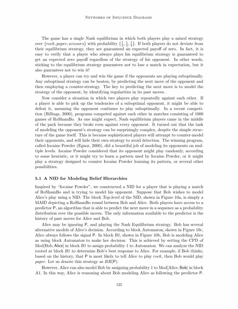
Inspired by “Iocaine Powder”, we constructed a NID for a player that is playing a matchof RoShamBo and is trying to model his opponent. Suppose that Bob wishes to modelAlice’s play using a NID. The block Top-level of the NID, shown in Figure 10a, is simply aMAID depicting a RoShamBo round between Bob and Alice. Both players have access to apredictor P, an algorithm that is able to predict the next move in a sequence as a probabilitydistribution over the possible moves. The only information available to the predictor is thehistory of past moves for Alice and Bob.
Alice may be ignoring P, and playing the Nash Equilibrium strategy. Bob has severalalternative models of Alice’s decision. According to block Automaton, shown in Figure 10c,Alice always follows the signal P. In block B1, shown in Figure 10b, Bob is modeling Aliceas using block Automaton to make her decision. This is achieved by setting the CPD ofMod[Bob, Alice] in block B1 to assign probability 1 to Automaton. We can analyze the NIDrooted at block B1 to determine Bob’s best response to Alice. For example, if Bob thinks,based on the history, that P is most likely to tell Alice to play rock, then Bob would playpaper. Let us denote this strategy as BR(P).
However, Alice can also model Bob by assigning probability 1 to Mod[Alice, Bob] in blockA1. In this way, Alice is reasoning about Bob modeling Alice as following the predictor P.
135
Gal & Pfeffer
P
bobalice
bob alice
Mod[Alice, Bob]
(a) Blocks Top-level, A1,A2
P
bobalice
bob alice
Mod[Bob, Alice]
(b) Blocks B1,B2
P
Alice
(c) Block Au-tomaton
Top-level
A2
B2
Bob,ALICE
Bob,ALICE
Automaton
Bob, ALICE
B1
Bob, ALICE
A1
Alice, BOB
Bob, ALICE
Alice, BOB
(d) RoShamBo NID
Figure 10: RoShamBo Scenario (Example 5.1)
136
Networks of Influence Diagrams
When we analyze the NID originating in block A1, shown in Figure 10a, we will determineAlice’s best-response to Bob’s model of her as well as Bob’s best-response to his model ofAlice. Since Alice believes that Bob plays BR(P) as a result of Bob’s belief that Alice playsaccording to P, she will therefore play a best response to BR(P), thereby double-guessingBob. Alice’s strategy in block A1 is denoted as BR(BR(P)). Following our example, inblock A1 Alice does not play rock at all, but scissors, in order to beat Bob’s play of paper.Similarly, in block B2, Bob models Alice as using block A1 to make her decisions, and inblock A2, Alice models Bob as using block B2 to make his decision. Therefore, solving theNID originating in block B2 results in a BR(BR(BR(P))) strategy for Bob. This wouldprompt Bob to play rock in B2 in our example, in order to beat scissors. Lastly, solvingthe NID originating in block A2 results in a BR(BR(BR(BR(P)))) strategy for Alice.This would prompt Alice to play paper in block A2, in order to beat rock. Thus, we haveshown that for every instance of the predictor P, Alice might play one of the three possiblestrategies. Any pure strategy can only choose between rock, paper, or scissors for anygiven P, so this reasoning process terminates.
The entire NID is shown in Figure 10d. In block Top-level, Bob models Alice as usingone of several possible child blocks: block Automaton, in which Alice follows her predictor;block A1, in which Alice is second-guessing her predictor; or block A2, in which Alice istriple-guessing her predictor. Bob’s uncertainty over Alice’s decision-making processes iscaptured in the Mod[Bob, Alice] node in block Top-level. Analyzing the Top-level block ofthis NID will extract Bob’s best response strategy given his beliefs about Alice’s decision-making processes.
To use this NID in practice, it is necessary to compute the MAID equilibrium and extractBob’s best-response strategy at the Top-level block. To this end, we need to estimate thevalues of the NID parameters, represented by the unknown CPDs at each of its blocks,and solve the NID. These parameters include Mod[Bob, Alice], representing Bob’s beliefsin the Top-level block regarding which block Alice is using; and node P, representing thedistributions governing the signals for Alice and Bob, respectively.2 To this end, we usean on-line version of the the EM algorithm that was tailored for NIDs. We begin withrandom parameter assignments to the unknown CPDs. We then revise the estimate overthe parameters of the NID given the observations at each round. Then Bob plays the best-response strategy of the MAID representation for the NID given the current parametersetting. Interleaving learning and using the NID to make a decision helps Bob to adapt toAlice’s possibly changing strategy.
5.2 Empirical Evaluation
We evaluated the NID agent against the ten top contestants from the first automaticRoShamBo competition. All of these agents used an opponent modeling approach, thatis, they learned some signal of their opponent’s play based on the history of prior rounds.Contestants can be roughly classified according to three dimensions: the type of signal used(probabilistic vs. deterministic); the type of reasoning used (pattern vs. meta-reasoners);and, their degree of exploration versus exploitation of their model. Probabilistic agents
2. Technically, the CPDs for the nodes representing prior history are also missing. However, they areobserved at each decision-making point in the interaction and their CPDs do not affect players’ utilities.
137
Gal & Pfeffer
estimated a distribution over the strategies of their opponents while deterministic agentspredicted their opponents’ next move with certainty. Pattern reasoners directly modeledtheir opponents as playing according to some rule or distribution, and did not reason aboutthe possibility that their opponents were modeling themselves. In contrast, meta-reasonersattempted to double- or triple-guess their opponents’ play. Exploitative agents played a bestresponse to their model of their opponents, while explorative agents deviated, under certainconditions, from their best response strategy to try and learn different behavioral patternsof their opponents. Iocaine Powder used the strategy of reverting to the Nash equilibriumwhen it was losing. Because this made it impossible to evaluate whether our NID modelcould learn Iocaine powder’s reasoning process, we turned off this strategy. Also, we limitedall contestants’ strategies to depend on the last 100 rounds of play, in order to allow a faircomparison with the NID agent that only used four rounds of play. We did not limit themto four rounds because they were not originally designed to use such a short history. Ourpurpose was to show that explicitly reasoning and learning about mental models can makea difference, and not to optimize learning the model of the signal.
Figure 11 shows the performance of the RoShamBo NID when playing 10 matches of3,000 rounds with each contestant. The overall standings were determined by orderingthe total scores for each contestant in all rounds played (+1 for winning a round against acontestant by the NID player; −1 for losing a round; 0 for ties). Therefore, it was importantfor each player to maximize its win against the weaker opponents, and minimize its loss tostronger opponents. The x-axis includes the contestant number while the y-axis describesthe difference between the average score of the RoShamBo NID and the contestant; errorbars indicate a single standard deviation difference.
As shown by the figure, the RoShamBo NID was able to defeat all contestant in allmatches, including a version of Iocaine Powder. The best performance for the NID wasachieved when playing pattern reasoners that used deterministic signals (Contestants 3, 5and 6). Each of these contestants directly predicted their opponents’ play as a function ofthe history, without reasoning about their opponents’ model of themselves. Consequently,it was difficult for them to detect change in the strategies of adaptive opponents, such asthe RoShamBo NID. In addition, the use of deterministic signals made it harder for thesecontestants to capture probabilistic players like the NID algorithm.
The RoShamBo NID also outperformed those contestants that attempted to trick theiropponents, by reasoning about the possibility that the opponents are double- and triple-guessing their model (Contestants 4 and 1). This shows that the NID was able to determinethe level of reasoning employed by its opponents.
6. Relationship with Economic Models
In this section, we describe the relationship between NIDs and several existing formalismsfor representing uncertainty over decision-making processes. NIDs share a close relation-ship with Bayesian games (Harsanyi, 1967), a game-theoretic framework for representinguncertainty over players’ payoffs. Bayesian games capture the beliefs agents have abouteach other as well as define an equilibrium that assigns a best response strategy for eachagent given its beliefs. Bayesian games are quite powerful in their ability to describe beliefhierarchies and cyclic belief structures.
138
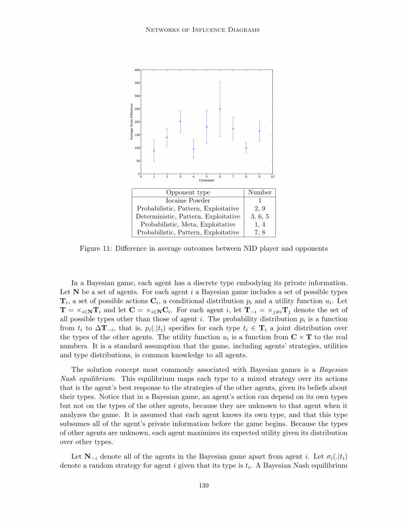
Networks of Influence Diagrams
0 1 2 3 4 5 6 7 8 9 100
50
100
150
200
250
300
350
400
Contestant
Ave
rage
Sco
re D
iffer
ence
Opponent type NumberIocaine Powder 1
Probabilistic, Pattern, Exploitative 2, 9Deterministic, Pattern, Exploitative 3, 6, 5
Probabilistic, Meta, Exploitative 1, 4Probabilistic, Pattern, Exploitative 7, 8
Figure 11: Difference in average outcomes between NID player and opponents
In a Bayesian game, each agent has a discrete type embodying its private information.Let N be a set of agents. For each agent i a Bayesian game includes a set of possible typesTi, a set of possible actions Ci, a conditional distribution pi and a utility function ui. LetT = ×i∈NTi and let C = ×i∈NCi. For each agent i, let T−i = ×j �=iTj denote the set ofall possible types other than those of agent i. The probability distribution pi is a functionfrom ti to ΔT−i, that is, pi(.|ti) specifies for each type ti ∈ Ti a joint distribution overthe types of the other agents. The utility function ui is a function from C × T to the realnumbers. It is a standard assumption that the game, including agents’ strategies, utilitiesand type distributions, is common knowledge to all agents.
The solution concept most commonly associated with Bayesian games is a BayesianNash equilibrium. This equilibrium maps each type to a mixed strategy over its actionsthat is the agent’s best response to the strategies of the other agents, given its beliefs abouttheir types. Notice that in a Bayesian game, an agent’s action can depend on its own typesbut not on the types of the other agents, because they are unknown to that agent when itanalyzes the game. It is assumed that each agent knows its own type, and that this typesubsumes all of the agent’s private information before the game begins. Because the typesof other agents are unknown, each agent maximizes its expected utility given its distributionover other types.
Let N−i denote all of the agents in the Bayesian game apart from agent i. Let σi(.|ti)denote a random strategy for agent i given that its type is ti. A Bayesian Nash equilibrium
139
Gal & Pfeffer
is any mixed strategy profile σ such that for any agent i and type ti ∈ Ti we have
σi(.|ti) ∈ argmaxτ∈ΔCi
∑t−i∈T−i
pi(t−i|ti)·∑c∈C
(∏j∈N−i
σj(cj |tj))τ(ci)ui(t, c)
(2)
Bayesian games have been used extensively for modeling interaction in which agents haveprivate information, such as auction mechanisms (Myerson, 1991) and they can be used toexpress uncertainty over agents’ decision-making models. In general, Bayesian games arejust as expressive as NIDs. As we show, any Bayesian game can be converted into a NIDin time and space linear in the size of the Bayesian game. Conversely, any NID can beconverted into a Bayesian game, because any NID can be converted to a MAID, which canin turn be converted to an extensive form game. The extensive form game can be convertedto a normal form game which is a trivial Bayesian game with only one type per agent.However, in the worst case, the size of the extensive form game will be exponential in thenumber of informational parents for decision nodes in the MAID, and the size of the normalform game will be exponential in the size of the extensive form game. Of course, this is abrute force conversion; more compact conversions may be possible.
We now consider more formally the question of whether Bayesian games can be repre-sented by NIDs. The idea is to align each type in a Bayesian game with a decision in aNID block. The resulting best response strategy for the decision in the NID equilibriumwill equal the Bayes Nash equilibrium strategy for the type.
Definition 6.1. Let B be a Bayesian game and N a NID. We say that N is equivalent toB if there exists an injective mapping f from types in B to (block,agent) pairs in N , suchthat the following conditions hold:
1. For any Bayesian Nash equilibrium σ of B, there exists a NID equilibrium of N , suchthat for every type ti, if f maps ti to (K, α), the best-response and actually-playedstrategies for α in K are equal to σi(.|ti).
2. For any NID equilibrium of N , there exists a Bayesian Nash equilibrium σ of B suchfor every (K, α) in the image of f , σi(.|ti) where ti = f−1(K, α) is equal to thebest-response and actually-played strategies for α in K.
The following theorem is proved in Appendix 8.
Theorem 6.2. Every Bayesian game can be represented by an equivalent NID whose sizeis linear in the size of the Bayesian game.
In this section, we will use the term Bayesian games to specify a representation thatincludes type distributions and utility functions that are presented explicitly. NIDs enjoy thesame advantages over fully specified Bayesian games that graphical models typically enjoyover unstructured representations. In general, NIDs may be exponentially more compactthan Bayesian games because Bayesian games require, for every type of every agent, a fulljoint distribution over the types of all other agents. In addition, the utility function in aBayesian game specifies a utility for each joint combination of types and actions of everyplayer. These distributions and utility functions are exponential in the number of players.In NIDs, because they are based on MAIDs, the type distributions can be decomposed
140
Networks of Influence Diagrams
into a product of small conditional distributions, and the utility functions can be additivelydecomposed into a sum of small functions that depend only on a small number of actions.
In addition, Bayesian games are representationally obscure. First, types in Bayesiangames are atomic entities that capture all the information available to an agent in a singlevariable. A type is used to capture both an agent’s beliefs about the way the world works(including its preferences), and its private information. For example, in poker, both theplayer’s beliefs about the other player’s tendency to bluff and her knowledge of what cardsshe has received are captured by a type. We believe that these two aspects are fundamentallydifferent; one describes the actual state of the world and the other describes what is going onin a player’s head. Conflating these two aspects leads to confusion. In NIDs, the two aspectsare differentiated. Private information about the world is represented by informationalparents, whereas mental models are represented by blocks.
Second, a type in a Bayesian game does not decompose different aspects of informationinto variables. Thus in poker, the hand must be represented by a single variable, whereas inNIDs it can be represented by different variables representing each of the cards. A final pointis that in Bayesian games all of the uncertainty must be folded into the utility functionsand the distribution over agents’ types. Consider the scenario in which two agents haveconflicting beliefs about a chance variable, such as in Example 4.3. In a NID, there willbe a separate block for each possible mental model that differs in the CPD assignmentsfor the chance variable. In contrast, each type in the Bayesian game would sum over thedistribution over the chance variable. Looking at the Bayesian game, we would not knowwhether the reason for the different utility functions is because the agent has different beliefsabout the chance variable, or whether it is due to different preferences of the agent.
NIDs also exhibit a relationship with more recent formalisms for games of awareness,in which agents may be unaware of other players’ strategies or of the structure of thegame (Halpern & Rego, 2006; Feinberg, 2004). A game description in this formalism showshow players’ awareness about each other’s strategies changes over time. A game of awarenessincludes a set of extensive form game descriptions, called augmented games, that representan analyst’s beliefs about the world, as well as separate descriptions for each game thatmay become true according to agents’ subjective beliefs. The analyst’s augmented game isconsidered to be the actual description of reality, while each subjective augmented game candiffer from the analyst’s game in agents’ utility functions, their decisions, and the strategiesavailable to agents at each of their decisions. A history for an agent in an augmented gameis a sub-path in the tree leading to a node in which the agent makes a move. Awareness ismodeled by a function that maps an agent-history pair in one augmented game to anotheraugmented game which the agent considers possible given the history. Uncertainty overagents’ awareness in an augmented game can be quantified by having nature choose amove in the tree leading to agents’ information sets. The definition of Nash equilibriumis extended to include a set of strategies for each agent-game pairthat the agent considersto be possible, given a history and the best-response strategies used by other agents in theaugmented game. This formalism can capture an analyst’s model about agents’ awarenessas well as agents’ model about their own, or other agents’ awareness.
There are fundamental differences between NIDs and games of awareness. First, likeBayesian games, the equilibrium conditions for this representation do not allow for agents todeviate from their best-response strategies. Second, they require the presence of a modeler
141

Gal & Pfeffer
agent, that in reality, is modeling its uncertainty about levels of awareness of other agents.NIDs allow for such a modeler agent, but they do not require it. This allows to capturesituations where no agent has certain knowledge of reality, such as in the Baseball NID ofExample 2.4. Third, each augmented game of awareness is represented as an extensive formgame, that as we have shown above, may be exponentially larger than the MAID used torepresent each decision-making model in a NID. Lastly, agents’ awareness over each other’sstrategies is just one type of reasoning that can be captured by a NID. Other types ofreasoning processes were described in Section 4.
Lastly, Gmytrasiewicz and Durfee (2001) have developed a framework for representinguncertainty over decision-making using a tree structure in which the nodes consist of payoffmatrices for a particular agent. Like Bayesian games, uncertainty is folded into the payoffmatrices. Each agent maintains its own tree, representing its model of the decision-makingprocesses used by other agents. Like traditional representations, this language assumes thatall agents behave rationally. In addition, it assumes that each agent believes others to usea fixed strategy, that is folded into the environment.
7. Conclusion
We have presented a highly expressive language for describing agents’ beliefs and decision-making processes in games. Our language is graphical. A model in our language is anetwork of interrelated models, where each mental model itself is a graphical model of agame. An agent in one mental model may believe that another agent (or possibly itself) usesa different mental model to make decisions; it may have uncertainty about which mentalmodel is used. We presented semantics for our language in terms of multi-agent influencediagrams. We analyzed the relationship between our language and Bayesian games. Theyare equally expressive, but NIDs may be exponentially more compact.
We showed how our language can be used to describe agents who play irrationally, in thesense that their actual play does not correspond to the best possible response given theirbeliefs about the world and about other agents. This is captured by a novel equilibriumconcept that captures the interaction between what agents should do and what they actuallydo. We also showed how to express situations in which agents have conflicting beliefs,including situations in which the agents do not have a common prior distribution over thestate of the world. Finally, we showed how to capture cyclic reasoning patterns, in whichagents engage in infinite chains of “I think that you think that I think...” reasoning.
A vital question is the use of our language to learn about agents’ behavior and reasoningprocesses. As we have shown, our language can be used to learn non-stationary strategiesin rock-paper-scissors. In other work, we have shown how models that were inspired byNIDs can learn people’s play in negotiation games (Gal, Pfeffer, Marzo, & Grosz, 2004; Gal& Pfeffer, 2006). The focus of our continuing work will be to develop a general method forlearning models in NIDs.
Acknowledgments
Thank you very much for the useful comments provided by the anonymous reviewers andeditor. Thanks to Barbara Grosz and Whitman Richards for their invaluable guidance.
142
Networks of Influence Diagrams
Thanks to Adam Juda for reading a prior draft of this work. This work was supported byan NSF Career Award IIS-0091815 and AFOSR under contract FA9550-05-1-0321.
8. Appendix A
Theorem 3.1: Converting a NID into a MAID will not introduce a cycle in the resultingMAID.
Proof. First, let us ignore the edges added by step 5 of the construction, and focus on theMAID fragment OK constructed from a single block K. Since the block is acyclic, we cannumber the nodes of the block with integers in topological order. We now number the nodesof OK as follows. For a node Nα that derives from a chance or utility node N in K, Nα
gets the same number as N . A node BR[D]K gets the same number as D. A node DKα ,
where α owns D, gets the same number as D plus 1/3. A node DKα , where α does not own
D, gets the same number as D plus 2/3. By construction, if P is a parent of N in OK , Phas a lower number than N .
Now let us consider the entire constructed MAID O. Suppose, by way of contradiction,that there is a cycle in O. It follows from the above argument that it must consist entirelyof edges between fragments added by step 5. Since all such edges emanate from a nodeDK
α where α owns D, and end at a node DLα , all nodes in the cycle must refer to the same
decision D, and must belong to the agent who owns D. Thus the cycle must be of the formDK1
α , . . . , DKnα , DK1
α where α owns D. Since an edge has been added from DKiα to DKi+1 in
O, α must be modeling itself in block Ki as using block Ki+1 to make decision D. Thereforethere is a self-loop in the NID, which is a contradiction.
Theorem 6.2: Every Bayesian game can be represented as an equivalent NID whose sizeis linear in the size of the Bayesian game.
Proof. Given a Bayesian game B, we construct a NID N as follows. The set of agents in Nis equal to the set of agents in B. For each type ti of agent i in B there is a correspondingblock in N labeled ti. The block ti contains a decision node Dj and utility node Uj forevery agent j. Dj has no informational parents. The domain of Dj is the set of choices Cj
for agent j in B. We add a new chance node Qi in block ti whose domain is the set T−i.Each node Mod[i, Dj ] where j �= i will have the node Qi as a parent. The parents of Ui areall the decision nodes as well as the node Qi. For an agent j �= i, Uj has only the parentDj . For each agent j we define a distinguished action c∗j ∈ Cj .
We set the CPD for nodes in ti as follows:
1. The CPD of Mod[i, Di] assigns probability 1 to ti.
2. The CPD of Qi assigns probability pi(t−i | ti), as defined in B, for each type profilet−i ∈ T−i.
3. The CPD of a node Mod[i, Dj ] where j �= i assigns probability 1 to block tj when thejth element of the value of the parent node Qi equals tj . This projects the probabilitydistribution Qi in B to the node Mod[i, Dj ] representing i’s beliefs about which blockagent j is using in the NID.
143
Gal & Pfeffer
4. The CPD of Ui assigns probability 1 to ui(t, c), as defined in B, given that Qi equalst, and D equals c.
5. The CPD of Uj assigns probability 1 to utility 1 when Dj = c∗j , and probability 1 to0 otherwise.
6. The CPD of Mod[j, Dk], for all k, when j �= i, assigns probability 1 to ti.
Our construction is accompanied by the injective mapping f that maps a type ti to the(block,agent) pair (ti, i).
Let M be the constructed MAID for N. To prove condition 1 of Definition 6.1, let τ bea Bayes Nash equilibrium of B. For each agent, τi is a conditional probability distributionτi(· | ti). We define the strategy profile σ in M as follows. σBR[Di]ti
= τi(· | ti) for decisionsowned by agent i, and σBR[Dj ]ti
assigns probability 1 to c∗j when j �= i.We claim the following:
1. σ is a MAID equilibrium in M, according to Definition 2.3.
2. In the resulting NID equilibrium, the best response strategy for i in ti is τi(· | ti).
3. In the resulting NID equilibrium, the actually played strategy is the same as the bestresponse strategy.
Claim 3 is true because Mod[i, Di] assigns probability 1 to ti.Note that there are no informational parents in N. Therefore, by the definition of NID
equilibrium, the best response strategy θtiDi
= σBR[Di,ti]= τi(· | ti). Therefore, Claim 2 is
true.To prove Claim 1, note first that in block ti, the utility node Uj , where j �= i, is fully
determined by Dj , because Dj is the sole parent of Uj . Also, player j is not self-modelingat Dj , because the CPD of node Mod[j, Dj ] assigns probability 1 to ti. The same holds inM: the decision node BR[Dj ]ti is the sole parent of U ti
j . Therefore, in any equilibrium forM, the strategy for BR[Dj ]ti will assign probability 1 to the distinguished action c∗j thatcauses U ti
j to be 1.In block ti, the CPD of Mod[i, Dj ] assigns probability 0 to ti. This means that player
j is not using block ti to make its decision, according to i’s beliefs. Therefore, BR[Dj ]tiis independent of U ti
i , and the equilibrium strategies for BR[Di]ti are independent of thedistinguished action chosen for the BR[Di]tj .
By the definition of MAID equilibrium of Definition 2.3, the strategy profile σ is anequilibrium if each σi maximizes EUσ(i). We need to show that maximizing this is equivalentto maximizing the right hand side of Equation 2. There is a utility U ti
i and decision nodeBR[Di]ti in every block ti. Let cti
i denote a choice for agent i at decision BR[Di]ti in block
ti. Let t′i denote a block corresponding to a different type t′i for agent i. Let ct′ii be a choice
for the agent in decision BR[Di]t′i at block t′i and c−i all the choices for other decisions
BR[D−i]ti . By the construction of M, U tii is d-separated from BR[Di]t
′i given BR[Di]ti and
BR[D−i]ti .As a result, we can optimize U ti
i separately from all other utility nodes belonging toagent i, considering only BR[Di]ti . We then get that the utility for i in M given the
144
Networks of Influence Diagrams
strategy profile σ can be written as
Eσ[U tii ] =
∑
ctii
σtii (cti
i )∑c−i
σ−i(c−i)∑
utii
P σ(U tii = ui | cti
i , c−i) · utii (3)
We now condition on agent i’s beliefs about the decisions of other agents in block ti. LetMod[i,D−i]ti denote the set of nodes Mod[i, Dj ]ti where j �= i, and let the tuple t−i referto the block label profile for blocks T−i. We now obtain
∑
ctii
σtii (cti
i )∑c−i
σ−i(c−i)∑t−i
P (Mod[i,D−i]ti = t−i)∑
utii
(utii | cti
i , c−i, t−i) · utii (4)
Now observe that the role of Mod[i,D−i]ti is to determine which choices for decisionsBR[D−i]ti are relevant for the utility of player i. In particular, if Mod[i, Dj ]ti is equal totj , then it is j’s choice in block tj that player i needs to consider when it makes decisionBR[Di]ti . Let ct−i
i denote the relevant choices for BR[D−i]ti when Mod[i,D−i]ti = t−i.Since other choice variables are irrelevant, we can marginalize them out and obtain
∑ctii
σtii (cti
i )∑
ct−i−i
σ−i(ct−i
−i )∑
t−iP (Mod[i,D−i]ti = t−i) (5)
∑u
tii
P σ(U tii = ui | cti
i , ct−i
−i ) · utii
Rearranging terms, we rewrite Equation 5.
∑t−i
P (Mod[i,D−i]ti = t−i)∑
c
(∏j �=i σ
tjj (ctj
j ))
(6)
σtii (cti
i )∑
utii
P σ(U tii = ui | cti
i , ct−i
−i ) · utii
By our construction, P (Mod[i,D−i]ti = t−i) is pi(t−i | ti) as defined in B, σtjj (ctj
j ) is
τj(cj | tj) as defined in B, and∑
utii
P σ(U tii = ui | cti
i , ct−i
−i ) · utii is ui(t, c). We therefore get
∑t−i
pi(t−i | ti)∑c
⎛⎝∏
j �=i
τj(cj | tj)
⎞⎠ τi(ci | ti)ui(t, c) (7)
Therefore σ is a MAID equilibrium of M if and only if τ is a Bayesian Nash equilibrium ofB. Claim 1 is established and therefore Condition 1 of Definition 6.1 is satisfied.
Finally, to prove Condition 2, given a NID equilibrium of N we construct a MAIDequilibrium σ for M by copying the best response strategies, and then construct strategiesτ for B in exactly the reverse manner to above. The previous reasoning applies in reverseto show that τ is a Bayes Nash equilibrium of B and the best response and actually playedstrategies for N are equal to τ .
145
Gal & Pfeffer
References
Arunachalam, R., & Sadeh, N. M. (2005). The supply chain trading agent competition.Electronic Commerce Research and Applications, 4, 63–81.
Aumann, R., & Brandenburger, A. (1995). Epistemic conditions for Nash equilibrium.Econometrica, 63 (5), 1161–1180.
Bazerman, M. (2001). Judgment in Managerial Decision Making. Wiley Publishers.
Billings, D. (2000). The first international RoShamBo programming competition. Interna-tional Computer Games Association Journal, 23 (1), 3–8.
Blum, B., Shelton, C. R., & Koller, D. (2006). A continuation method for Nash equilibriain structured games. Journal of Artificial Intelligence Research, 25, 457–502.
Bonanno, G., & Nehring, K. (1999). How to make sense of the common prior assumptionunder incomplete information. International Journal of Game Theory, 28, 409–434.
Camerer, C. F. (2003) In Behavioral Game Theory. Experiments in Strategic Interaction,chap. 2. Princeton University Press.
Cowell, R. G., Lauritzen, S. L., & Spiegelhater, D. J. (2005). Probabilistic Networks andExpert Systems. Springer.
Dechter, R. (1999). Bucket elimination: A unifying framework for reasoning. ArtificialIntelligence, 113 (1-2), 41–85.
Egnor, D. (2000). Iocaine Powder. International Computer Games Association Journal,23 (1), 3–8.
Feinberg, Y. (2004). Subjective reasoning — games with unawareness. Tech. rep. 1875,Stanford University.
Gal, Y., & Pfeffer, A. (2003a). A language for modeling agents’ decision making processesin games. In Proc. 2nd International Joint Conference on Autonomous Agents andMulti-agent Systems (AAMAS).
Gal, Y., & Pfeffer, A. (2003b). A language for opponent modeling in repeated games. InWorkshop on Game Theory and Decision Theory, AAMAS.
Gal, Y., & Pfeffer, A. (2004). Reasoning about rationality and belief. In Proc. 3rd Interna-tional Joint Conference on Autonomous Agents and Multi-agent Systems (AAMAS).
Gal, Y., & Pfeffer, A. (2006). Predicting people’s bidding behavior in negotiation. In Proc.5th International Joint Conference on Autonomous Agents and Multi-agent Systems(AAMAS).
Gal, Y., Pfeffer, A., Marzo, F., & Grosz, B. (2004). Learning social preferences in games.In Proc. 19th National Conference on Artificial Intelligence (AAAI).
Gigerenzer, G., & Selten, R. (Eds.). (2001). Bounded Rationality: The Adaptive Toolbox.MIT Press.
Gmytrasiewicz, P., & Durfee, E. H. (2001). Rational communication in multi-agent envi-ronments. Autonomous Agents and Multi-Agent Systems, 4 (3), 233–272.
146
Networks of Influence Diagrams
Halpern, J., & Rego, L. (2006). Extensive games with possibly unaware players. In Proc.5th International Joint Conference on Autonomous Agents and Multi-agent Systems(AAMAS).
Harsanyi, J. C. (1967). Games with incomplete information played by ’Bayesian’ players.Management Science, 14, 159–182, 320–334, 486–502.
Howard, R. A., & Matheson, J. E. (1984). Influence diagrams. In Readings on the Principlesand Applications of Decision Analysis, pp. 721–762.
Kearns, M., Littman, M., & Singh, S. (2001). Graphical models for game theory. In Proc.17th Conference on Uncertainty in Artificial Intelligence (UAI).
Koller, D., Meggido, N., & von Stengel, B. (1996). Efficient computation of equilibria forextensive two-person games. Games and Economic Behavior, 14 (2), 247–259.
Koller, D., & Milch, B. (2001). Multi-agent influence diagrams for representing and solvinggames. In Proc. 17th International Joint Conference on Artificial Intelligence (IJCAI).
MacKie-Mason, J. K., Osepayshivili, A., Reeves, D. M., & Wellman, M. P. (2004). Priceprediction strategies for market-based scheduling. In Proc. of 18th International Con-ference on Automated Planning and Scheduling.
Morris, S. (1995). The common prior assumption in economic theory. Economic Philosophy,pp. 227–253.
Myerson, R. (1991). Game Theory. Harvard University Press.
Pearl, J. (1988). Probabilistic Reasoning in Intelligent Systems. Morgan Kaufmann.
Rajarshi, D., Hanson, J. E., Kephart, J. O., & Tesauro, G. (2001). Agent-human interactionsin the continuous double auction. In Proc. 17th International Joint Conference onArtificial Intelligence (IJCAI).
Rubinstein, A. (1998). Modeling Bounded Rationality. MIT Press.
Russell, S., & Wefald, E. (1991). Do the Right Thing: Studies in Limited Rationality. MITPress.
Simon, H. A. (1955). A behavioral model of rational choice. Quarterly Journal of Economics,69, 99–118.
Vickrey, D., & Koller, D. (2002). Multi-agent algorithms for solving graphical games. InProc. 18th National Conference on Artificial Intelligence (AAAI).
147


![Atlas of phase diagrams - COST 531 (Lead-free solders)...‐8‐ COST 531‐ Atlas of phase diagrams is given by the Muggianu extension of the Redlich‐Kister formalism [75Mug, 48Red]](https://img.pdfslide.net/doc/110x75/610c774a76033d735049e9f8/atlas-of-phase-diagrams-cost-531-lead-free-solders-a8a-cost-531a-atlas.jpg)