Arthur J. DeckerGlenn Research Center, Cleveland, Ohio

Neural-Net Processed Electronic Holographyfor Rotating Machines

NASA/TM—2003-212218

February 2003

https://ntrs.nasa.gov/search.jsp?R=20030019354 2018-07-13T01:10:44+00:00Z

The NASA STI Program Office . . . in Profile

Since its founding, NASA has been dedicated tothe advancement of aeronautics and spacescience. The NASA Scientific and TechnicalInformation (STI) Program Office plays a key partin helping NASA maintain this important role.

The NASA STI Program Office is operated byLangley Research Center, the Lead Center forNASA’s scientific and technical information. TheNASA STI Program Office provides access to theNASA STI Database, the largest collection ofaeronautical and space science STI in the world.The Program Office is also NASA’s institutionalmechanism for disseminating the results of itsresearch and development activities. These resultsare published by NASA in the NASA STI ReportSeries, which includes the following report types:

• TECHNICAL PUBLICATION. Reports ofcompleted research or a major significantphase of research that present the results ofNASA programs and include extensive dataor theoretical analysis. Includes compilationsof significant scientific and technical data andinformation deemed to be of continuingreference value. NASA’s counterpart of peer-reviewed formal professional papers buthas less stringent limitations on manuscriptlength and extent of graphic presentations.

• TECHNICAL MEMORANDUM. Scientificand technical findings that are preliminary orof specialized interest, e.g., quick releasereports, working papers, and bibliographiesthat contain minimal annotation. Does notcontain extensive analysis.

• CONTRACTOR REPORT. Scientific andtechnical findings by NASA-sponsoredcontractors and grantees.

• CONFERENCE PUBLICATION. Collectedpapers from scientific and technicalconferences, symposia, seminars, or othermeetings sponsored or cosponsored byNASA.

• SPECIAL PUBLICATION. Scientific,technical, or historical information fromNASA programs, projects, and missions,often concerned with subjects havingsubstantial public interest.

• TECHNICAL TRANSLATION. English-language translations of foreign scientificand technical material pertinent to NASA’smission.

Specialized services that complement the STIProgram Office’s diverse offerings includecreating custom thesauri, building customizeddatabases, organizing and publishing researchresults . . . even providing videos.

For more information about the NASA STIProgram Office, see the following:

• Access the NASA STI Program Home Pageat http://www.sti.nasa.gov

• E-mail your question via the Internet tohelp@sti.nasa.gov

• Fax your question to the NASA AccessHelp Desk at 301–621–0134

• Telephone the NASA Access Help Desk at301–621–0390

• Write to: NASA Access Help Desk NASA Center for AeroSpace Information 7121 Standard Drive Hanover, MD 21076

Arthur J. DeckerGlenn Research Center, Cleveland, Ohio

Neural-Net Processed Electronic Holographyfor Rotating Machines

NASA/TM—2003-212218

February 2003

National Aeronautics andSpace Administration

Glenn Research Center

Available from

NASA Center for Aerospace Information7121 Standard DriveHanover, MD 21076

National Technical Information Service5285 Port Royal RoadSpringfield, VA 22100

This report is a formal draft or workingpaper, intended to solicit comments and

ideas from a technical peer group.

Trade names or manufacturers’ names are used in this report foridentification only. This usage does not constitute an officialendorsement, either expressed or implied, by the National

Aeronautics and Space Administration.

Available electronically at http://gltrs.grc.nasa.gov

NASA/TM—2003-212218 iii

TABLE OF CONTENTS

SUMMARY.............................................................................................................. iv

INTRODUCTION..................................................................................................... 1

TECHNICAL JUSTIFICATION FOR ATTEMPTING ROTATING STAGE ............... 3 HOLOGRAPHY

THE OPERATIONAL ENVIRONMENT ...................................................................15

SOFTWARE AND COMPUTER SUPPORT............................................................16

CAMERAS AND LASERS.......................................................................................17

METHODS AND SETUPS ......................................................................................18

PREFACE ....................................................................................................18

NEURAL-NET INSPECTION TECHNIQUE..................................................19

DATA ACQUISITION, PREPARATION AND CONDITIONING ....................26

SHORT-EXPOSURE DOUBLE-EXPOSURE HOLOGRAMS AS AN EXAMPLE OF HOW TO HANDLE TWO INDEPENDENT RANDOM PROCESSES IN TRAINING NEURAL NETS ..............................................33

FIBERSCOPE ELECTRONIC HOLOGRAPHY.......................................................36

FUNDAMENTALS OF FIBERSCOPE HOLOGRAPHY................................36

NEURAL-NET PROCESSED CHARACTERISTIC PATTERNS OF A

BLISK ...........................................................................................................39

HIGH-SPEED HOLOCAMERAS.............................................................................42

MOST IMPORTANT PERFORMANCE CRITERION....................................42

CORRELATION COEFFICIENTS ................................................................43

PERFORMANCE OF THE IMAGE INTENSIFIER FOR ELECTRONIC

HOLOGRAPHY ............................................................................................44

PULSED-LASER HOLOGRAMS..................................................................49

SUMMARY AND DISCUSSION OF RESULTS.......................................................52

CONCLUSIONS AND CONCLUDING REMARKS..................................................54

REFERENCES........................................................................................................54

NASA/TM—2003-212218 iv

SUMMARY

This report presents the results of an R&D effort to apply neural-net processed electronic holography to NDE of rotors. Electronic holography was used to generate characteristic patterns or mode shapes of vibrating rotors and rotor components. Artificial neural networks were trained to identify damage-induced changes in the characteristic patterns. The development and optimization of a neural-net training method were the most significant contributions of this work. A training set was first assembled from the vibration mode shapes of an undamaged structure. The structure could then be subjected to potentially destructive testing, and the onset of damage could be detected The training method and its optimization are discussed in detail. A second positive result was the assembly and testing of a fiber-optic holocamera. A 20-foot fiberscope was used to relay images of the rotor component to be tested. These images were then used to form focused-image holograms for recording by a CCD camera. The fiberscope can be inserted into a test facility such as the Glenn Spin Rig for remote acquisition of the image of the rotor component to be inspected. The implementation and performance of fiberscope holography are discussed in detail. A major disappointment was the inadequacy of the high-speed-holography hardware selected for this effort. Holograms must be recorded in tens of nanoseconds at the highest speeds. Longer exposures can be used for the slower moving parts of the rotor. There was an attempt to use image-intensified holography with a continuous-wave laser to meet the high-speed requirement. The actual approach was quite interesting. Scaled holograms were used to match the low effective resolution of the intensifier. A minimum exposure time of 25 microseconds was achieved at a continuous-wave-laser power of about 1 Watt, but the exposure time was still 2 to 3 orders of magnitude too large for moving-rotor holography. An old pair of injection-seeded Nd:YAG lasers produced short enough exposures of 5 nanoseconds, but did not produce adequately correlated double holograms. The results of these high-speed efforts are presented. This report also discusses in some detail the physics and environmental requirements for rotor electronic holography. A key performance specification based on correlations is discussed. The NDE of a non-rotating blisk is reported as an example. Both the optical access of the root region and the repeatability of vibration excitation of the blisk proved to be difficult. The major conclusions were that neural-net and electronic-holography inspections of stationary components in the laboratory and the field are quite practical and worthy of continuing development, but that electronic holography of moving rotors is still an expensive high-risk endeavor.

NASA/TM—2003-212218 1

Neural-Net Processed Electronic Holography for Rotating Machines

Arthur J. Decker National Aeronautics and Space Administration

Glenn Research Center Cleveland, Ohio 44135

INTRODUCTION

An R&D project was conducted in fiscal years 1999 through 2001 at NASA

Glenn with the objective: to develop neural-net processed, time-average and double-exposure electronic holography to detect blade damage in a rotating stage, thereby extending whole-field, non-intrusive, fast damage-inspection to a rotating turbo-machine component.

The project was intended to be a follow-on to a NASA-Lewis Director’s Discretionary Fund project to use neural-nets to process electronic holograms to visualize damage and strain information in fan blades.1–4 The DDF project was concerned mainly with detecting structural damage in the laboratory, although it also had the ultimate objective of being adapted to on-site inspections of turbo-machine components.

Both projects were justified to NASA to promote safety in the operation of ground test facilities or aviation safety, in general. There is value in being able to detect the gradual on-set of structural changes or structural damage in a turbo-machine component or other structural component. Such changes possibly can occur when the component is operated outside its design envelope, where said operation might occur frequently in a ground-test facility. Or changes might occur for unforeseen reasons in a component being tested or operated normally. It is inconvenient, and possibly expensive, to remove the component to a laboratory for testing, although that approach has been used for holographic testing at Lewis, and then Glenn, for about 30 years. Hence, the development of non-intrusive, on-site, optical inspection systems such as neural-net-processed electronic holography is justified.

Neural-net-processed electronic holography of machine components offers significant potential advantages over other methods. It is non-intrusive; since a component need not be loaded with gauges. It is a whole-field technique; since a substantial fraction of the surface of a component can be monitored. In fact, the vibration-determined patterns that are detected using neural-net processed holography can be affected by spatially remote events; hence neural-net processed electronic holography can be used, in principle, for health monitoring.

The adaptation of holographic techniques to objects experiencing center-of-mass motion is a major undertaking and not to be taken lightly. It has been attempted from time to time since the days of silver-halide-emulsion holography.5–6 Recently, the practical developments of electronic interferometry and electronic holography have generated new interest in rotating machine applications.7–9 And artificial neural networks have been used to overcome a

NASA/TM—2003-212218 2

major limitation on the applications of holographic structural analysis. Specifically the interpretation of holographic data is tedious or difficult, and the data are often noisy with information about the structural defects buried in complex fringe patterns. But neural nets have been applied to the routine automated detection of structural damage as recorded using noisy electronic holograms.10 Interpretation of these holograms for structural damage is now accomplished by the neural nets without the intervention of a human operator.

Nevertheless there are severe constraints on whether holography of moving objects can be effective and affordable. These constraints are determined by fundamental optical principles, and by the availability of appropriate laser and detector technologies. This R&D project was only partly successful in meeting the constraints, although the initial estimates of risk indicated that meeting the constraints was worth a try.

A first risk is that structural and flow fluctuations interact in generating the fringe patterns. This complicating effect was noted during one of the historical attempts to use silver-halide holographic interferometry to measure vibration properties in of a rotating fan stage.6 Consequently, the decision at Glenn was to restrict the study to the Glenn Spin Rig. Rotation in a spin rig occurs in vacuum, and aerodynamic effects don’t exist. Even laboratory applications and applications to stationary objects in the field are affected somewhat by a fluctuating atmosphere.

A second risk is achieving adequate optical access. The access in the case of a spin rig must maintain vacuum integrity. The classical approach is to use windows, but window vibration can introduce interference fringes. Good windows of significant size are expensive. The decision was to use fiber-optic access instead. There is not much experience in performing holography through fiber-optic bundles, so that this technique created its own risks. But the fiber-bundle technique worked fairly well and must be considered one of the successes of the project. Nevertheless, fiber optics degrades the holographic process, and introduces factors that reduce performance.

A third risk of holography has been to achieve adequate interpretation of the interference-fringe patterns. Converting a pattern to a physical quantity such as a displacement distribution does not eliminate the need for sensible interpretation. Automated interpretation of the patterns using neural networks was used to control this risk. Neural-net interpretation uses complete images, but provides definitive answers and decisions to users not versed in optics. In fact, the sensitivity of fringe interpretation was increased considerably during the project using a technique called folding.11–12 Neural-net interpretation was applied to inspection of an International Space Station cold plate.10 Hence the improvement in neural-net interpretation must be considered one of the successes of the project.

The fourth and greatest risk is finding the illumination and recording systems that satisfy the optical constraints. The field known as particle image velocimetry or PIV has resulted in the development of sophisticated, but very expensive, illumination and recording systems. The importance of velocity measurements in fluid dynamics justified that effort and expense. Therefore, the

NASA/TM—2003-212218 3

pulsed lasers, cameras and controlling computer systems of PIV were available commercially, but were felt to be too expensive for the finances of the project. And it was uncertain that even the PIV hardware and software would be adequate. Instead the decision was to use an image intensifier and continuous wave lasers to achieve the short exposure times demanded by the project. A technique known as frame straddling13 also developed for PIV was used to capture pairs of holograms separated by a short time. This approach failed because the image intensifier did not have enough resolution. Nevertheless, image-intensifier holograms were recorded and constitute an achievement at least of academic interest.14

The fifth risk that was never fully investigated was whether the optical constraints would be satisfied adequately even with ideal equipment. The judgment was that adequate holograms could not be recorded with the image intensifier, continuous-wave-laser, and fiber-bundle combinations. Further R&D would have required using a test facility (Spin Rig) for an extended period of time as a research instrument. Nevertheless, some preliminary inspections of a bladed disk (blisk) showed that it was challenging to excite the vibration modes of the blades repeatably enough to use the neural-net inspection methods.

This TM discusses the design and evaluation of the fiber-bundle, frame-straddled, image-intensified, and neural-net-processed electronic holography systems intended for damage detection in a rotating stage. The paper begins, however, with a discussion of the optical constraints for recording electronic holograms of rotating stages. It is legitimate to ask whether any existing technology has a reasonable chance to perform this recording procedure adequately.

TECHNICAL JUSTIFICATION FOR ATTEMPTING ROTATING STAGE HOLOGRAPHY

There are several observations and assumptions that we make. Dändliker

provides a theory to be used to discuss some of these assumptions.15 His discussion in fact pertains to silver-halide-emulsion heterodyne holographic interferometry; whereas this paper is solely concerned with phase shifting electronic holography. Nevertheless Dändliker’s analysis can be adapted quite easily and combined with some other observations. The major assumption behind all this work, that neural nets can be trained to handle many potentially confusing and extraneous effects and noise sources, will be left until the end of this section. A systematic treatment of the structure of training sets is left to the section on double-exposure holograms.

The first assumption or observation is that the surfaces to be inspected have sub-wavelength roughness. Specifically, mirror-surface reflections are assumed not to exist or not to be detected. Only the light scattered by the nano-structure of the surface is assumed to reach the detector. The simplest concept is that the surface is composed of independent Rayleigh scatterers. The light from each scatterer is assumed to reach all parts of the limiting aperture of the holographic system.

NASA/TM—2003-212218 4

The second assumption in electronic holography is that the pupil of a CCD camera lens is the limiting aperture. That aperture in turn imposes a spatial resolution. That is, the waves from the scatterers within a small area or resolved spot of the surface are added by convolution with a function known as the impulse response function of the CCD lens and pupil combination. In the optics of propagating light, the minimum characteristic size of the area from which scattered waves can be added is approximately a wavelength of light (about 500 nanometers). The actual size from a stopped-down CCD lens is much larger. Through magnification, the minimum size of the resolved area on the structure itself can be even larger. The geometry of this area depends on the shape of the aperture, the aberrations, and to some extent on the statistical properties of the surface nano-structure. A simple circular aperture with a perfect imaging lens is selected for purposes of estimation and justification. The classical resolved diameter of the area on the surface is then given by

MDs1.2 dO λ= (1)

Here, λ is the wavelength of the light used (532 nm is common); s is the distance from the aperture to the image on the CCD array; D is the diameter of the aperture; M is the magnification factor in going from the image to the object; and do is the diameter of a resolved spot on the object. For those applications where the image is near the focal plane of the lens, eq. (1) becomes a more familiar expression to anyone acquainted with photographic techniques: FM1.2 do λ= (2) Here F is the f-number of the lens. As an example, suppose that a 1 m diameter blisk is imaged onto a 10 mm x 10 mm CCD array by an f/10 lens. Then do = 0.6 mm. In electronic holography, a reference beam is superimposed on the image to form a so-called image-plane hologram. The lens acts like a light-ray angle selector called a spatial filter. The imaging system in electronic holography low-pass-filters the spatial frequencies that then form the interference pattern between the image and reference beams. A significant, but not total, amount of the power in the interference term is then associated with spatial frequencies small enough to be resolved by a CCD array. The intensity and phase of the resolved spots in the focused image itself are random variables built up from the random nano-structure of the surface. The randomness constitutes the laser speckle effect. The third assumption is that the speckle pattern moves intact as an object moves or rotates, at least for the short time between two holograms. The aperture does not change, and the illumination direction and illumination properties are assumed not to change much. The viewing direction is also assumed not to change much. The nano-structure of the surface moves with the surface. Needless to say, violations of these assumptions will degrade the correlation between speckle patterns. For example, the speckle patterns from

NASA/TM—2003-212218 5

two different aperture sizes are uncorrelated. One way to hold the illumination and viewing directions constant is to place the illumination source and detector near the axis of a rotator. The fourth assumption is that holograms are to be compared between two states of a rotor recorded by electronic holography at two different times, or continuously by time averaging. The two states are recorded electronically using a pair of holograms. A pair of holograms (at least) is also required for time averaging. The rotor is assumed to vibrate, and its vibration-displacement distribution is assumed to change in time.

Figure 1—Holographic Arrangement Figure 2—Nearly Circular For Motion Along Ellipse. Motion. The fifth assumption (really an observation or principle) is that the macroscopic phase change between the two states of the rotor is caused mainly by out-of-rotor-plane motion. Figure 1 shows the geometry where the assumption is exact. An object, assumed to be of negligible extent, is shown moving along an ellipse with the laser light source at one focus and the detector at the second focus. The inter-hologram phase change from said motion is exactly zero; since the sum of the distances between a point on the ellipse and the two foci is constant. Only motion perpendicular to the ellipse results in a phase change. Imagine a rotor blade that is moving tangent to the ellipse. Then for a brief period the rotation does not cause a phase change at the point of tangency. But vibration of the blade perpendicular to the tangent plane does cause a phase change. The holodiagram that predicts fringes patterns from different kinds of motion between ellipsoids exploits this effect.16 Consider a source and a detector so close together that the ellipse is nearly a circle as in figure 2, and suppose that the radius of the circle is 0.5 m. Then the tangent point of the blade will need to travel 0.5 mm (1000 waves) along the tangent plane before the effect is equivalent to a perpendicular motion of one wavelength. It is interesting to note that 0.5 mm is equal to the size of a resolution element calculated in the example above. Rotation-induced fringes are potentially a problem even with an optimum

NASA/TM—2003-212218 6

geometry. Image de-rotating prisms have been used to compensate for rotation-induced fringes, but they must be used on the rotation axis. A more serious problem is that the phase changes slowly only at the tangent point. A sixth assumption or observation is that definite or macroscopic comparisons are possible only between the same speckles (corresponding resolved spots) on the two holograms. Different speckles have a random phase relationship, where the phase in a hologram is recorded because of the presence of a reference beam. The macroscopic interference effect contains the information about the structure and its integrity. A definite or macroscopic inter-hologram phase relationship is measured only when the inter-hologram tangential motion of the speckles is less than about a speckle diameter. Comparisons by means of interferometry of reconstructed waves or differencing of electronic holograms suffer from reduced contrast or errors when the corresponding speckles don’t overlap exactly. The information about structural motion will be lost completely, if the relative tangential motion is too great. The single speckle interference effect can be calculated15 by adapting Dändliker’s approach. Two overlapping resolution elements formed by the CCD lens at slightly different times have fields given by the object waves va V 11 = (3)

γ+γ= ϕ w)-(1 veaV 2

12i

22 (4)

The useful information is contained entirely in the complex exponential φie . The phase introduced by the corresponding displacement of a point on the structural surface occurring between the two hologram recordings is given by

δ•λπ

=φ K2 (5)

In equation (5), the vector K is the difference between unit vectors from the imaged point to the center of the CCD lens pupil and from the illumination source to the imaged point. Sometimes K is called the sensitivity vector. The wavelength of the light used is again denoted by λ (very typically 0.532 µm from the frequency-doubled neodymium-ion lasers that have become so common), and the vector displacement including the rotation contribution is given by δδδδ. Displacements of a micrometer or less can be important. We have already mentioned that the component of the sensitivity vector along the tangential motion is small relative to component along the perpendicular motion.

The complex random variables v and w are normalized, uncorrelated and Gaussian random variables in Dändliker’s approach. The variable γ measures the averaged fringe contrast in silver-halide double-exposure holography or the correlation coefficient of displaced speckle patterns in general and is given by

NASA/TM—2003-212218 7

II

II1

d/Du)d/Du(J2

λπλπ

=γ (6)

where J1 is a first-order Bessel Function of the first kind. Here, uI is the transverse inter-hologram displacement or mutual shift of the speckle patterns, dI is the distance of the image from the lens, and D is the diameter of the imaging aperture as before.

The correlation γ varies from 1 to 0. When γ=1, eqs. (3) and (4) yield the simplest expressions vaV 11 = (7) φ= i

22 veaV (8) Generally a1 = a2, and double-exposure electronic holography will yield a simple fringe pattern. The same reference beam R is used for both holograms. The first hologram for a single speckle (resolution spot) is given by *

11*22

12

1 Ra vaR va R H v+++= (9) when γ = 1. The second is given by ϕφ -i*

1i

1*22

12

2 evRa veaR va R H +++= (10) when a1 = a2. Note that v2 is to be interpreted as vv*; since v is a complex variable. The real and imaginary parts of v are normally distributed, and that assumption yields the most common way of modeling the laser speckle effect. The holograms are simply subtracted, when they are recorded using electronic holography, to yield the result )e - (1vRa )e-v(1aR H-H -i*

1i

1*

21φφ += (11)

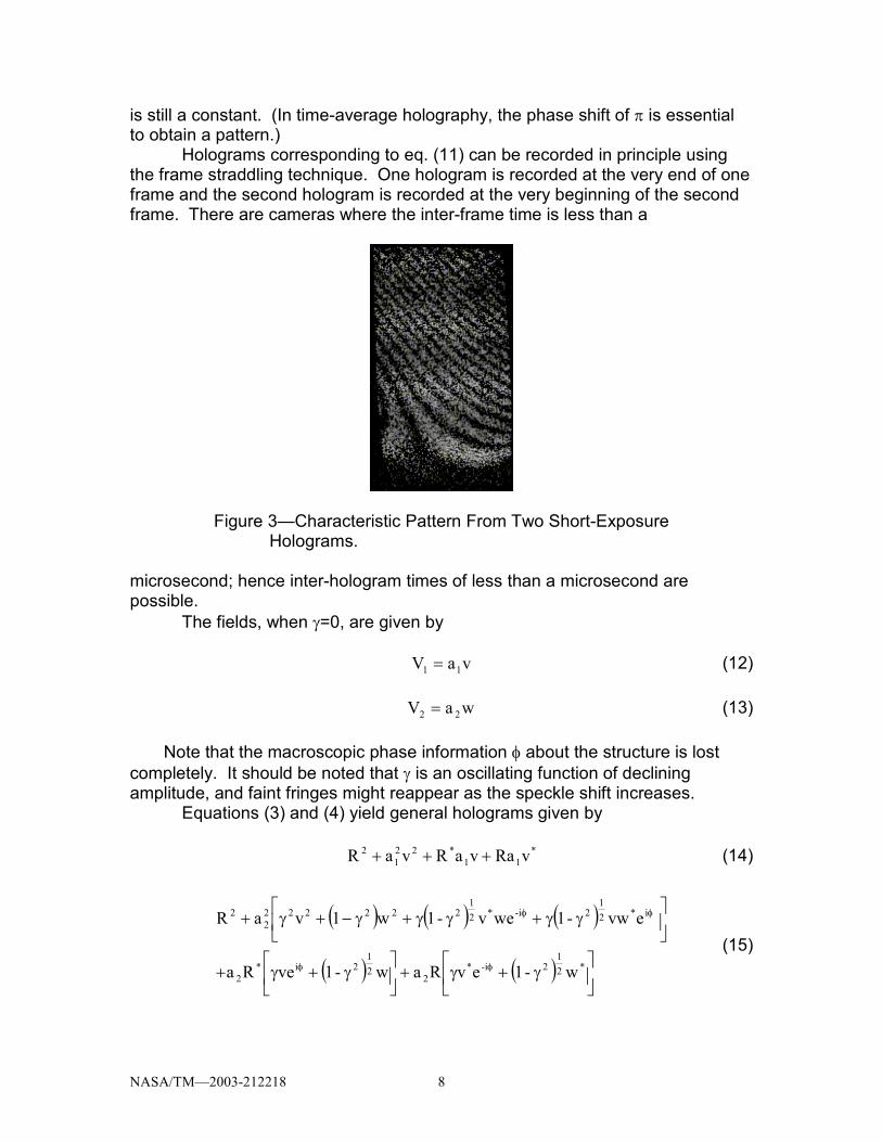
This process is to be contrasted with silver-halide holography, where the two waves are reconstructed simultaneously and interfere. Subtraction removes the so-called high frequency or self-interference terms and greatly improves the contrast for visualizing the cross-interference effect. The resulting pattern yields a dark fringe for no phase change (ϕ=0) and yields dark fringes also for phase changes that are integer multiples of 2π. The fringes are bright when the phase change is an odd-integer multiple of π. Figure 3 shows an example from two holograms recorded of a vibrating blade. Shifting the phase of the reference beam by π between holograms will transfer a bright fringe to the zero-phase condition, but the contrast of the electronic fringes

NASA/TM—2003-212218 8

is still a constant. (In time-average holography, the phase shift of π is essential to obtain a pattern.) Holograms corresponding to eq. (11) can be recorded in principle using the frame straddling technique. One hologram is recorded at the very end of one frame and the second hologram is recorded at the very beginning of the second frame. There are cameras where the inter-frame time is less than a

Figure 3—Characteristic Pattern From Two Short-Exposure Holograms. microsecond; hence inter-hologram times of less than a microsecond are possible. The fields, when γ=0, are given by vaV 11 = (12) waV 22 = (13) Note that the macroscopic phase information φ about the structure is lost completely. It should be noted that γ is an oscillating function of declining amplitude, and faint fringes might reappear as the speckle shift increases. Equations (3) and (4) yield general holograms given by *

11*22

12 vRa vaR va R +++ (14)

( ) ( ) ( )

( ) ( )

γ+γ+

γ+γ+

γγ+γγ+γ−+γ+

φφ

φφ

*21

2i-*2

21

2i*2

i*21

2i-*21

2222222

2

w-1evRaw-1veRa

evw-1 wev-1w1va R (15)

NASA/TM—2003-212218 9

Subtracting the holograms eliminates the reference intensity. The useful information contained by φ remains, but is corrupted by other terms. The reference intensity can be made large relative to the intensity from the object, thereby increasing the relative importance of the last two terms, after hologram subtraction. The result after hologram subtraction is given approximately by

[ ] [ ] ( ) [ ]**2

21

221

*21

* RwwRa-1a -aRv a-avR +−+ − γγγ φφ ii ee (16) Equations (11) and (16) yield expressions that are not improved by averaging; since v and w are both zero-mean random variables. In silver-halide holography, the signal terms are multiplied by interference during reconstruction (thereby creating unity average v*v terms); hence averaging of many pixels within the final-detector aperture or averaging many holograms will improve the signal-to-noise in silver-halide holography. The processing steps in frame-straddled electronic holography normally don’t use a multiplication process (four holograms would be necessary to provide two differences for multiplication). But, subtracting a single pair of frame-straddled electronic holograms leaves nothing for a multiplication step. The remaining choices are to evaluate the absolute values of pixels obtained from expressions (11) or (16), or to square the pixels. The absolute value operation was selected for the work reported in this paper. Averaging can then be accomplished to improve the electrical signal-to-noise ratio or to average varying speckle patterns, or the averaging property of feed forward artificial neural networks can be exploited. Even severe de-correlation is not necessarily a disaster in silver-halide or electronic holography, if the de-correlation is caused merely by a speckle-pattern shift. Said de-correlation simply leads to a change in the apparent interference-fringe position in 3-d space in silver-halide holography (the fringe localization effect). And one can de-rotate the holograms computationally in electronic holography, if the motion is truly one of rigid rotation. This procedure is the computational equivalent of sandwich holography. However, macroscopic rotation fringes cannot be removed in this manner in electronic holography. A seventh convenient assumption for illustration purposes is that the exposure times and inter-exposure times will be kept small enough for 75.0≥γ as in Dändliker’s formalism. It was noted above that the requirements for controlling rotation fringes (at the tangent point of the ellipse) and de-correlation were comparable; hence, this illustrative lower value for γ is assumed to assure adequate values for both. The question then is whether this requirement corresponds to reasonable times for attempting electronic holography of a rotating stage. The answer of course has to be yes in principle; since the speed due to rotation varies from zero at the center to the maximum value at the rim. As discussed below, neural nets have proven to be sensitive enough to detect damage occurring in a location outside the optically detected region. Hence, in principle, the recording point need only be moved toward the shaft until the rotor linear speed is small enough to be recorded. The neural net then monitors the local pattern, and detects both local and remote changes and damage. In any

NASA/TM—2003-212218 10

case, the exposure time can be plotted as a function of speed to see whether a reasonable fraction of a rotor can be recorded at a realistic speed. The general formula for an inter-exposure time between holograms, corresponding to γ=0.75, is given by

VD

s0.5Mt λ=∆ (17)

or by

V

F0.5Mt λ=∆ (18)

The second equation is used when the image is near the focus of the CCD lens. The linear speed is denoted by V and varies, of course, with the radial position on the rotor. Figure 4 shows the inter-exposure time plotted against V for the rotor used to discuss eq. (2). There M = 100, λ= 0.532x10–6 m, and F = 10. µsec

m/s Figure 4—Inter-Exposure Time Versus Speed. The tolerable inter-exposure time varies from 266 microseconds at the rather low speed of 1 m/sec to 0.2 microseconds at the formidable speed of 1330 m/sec. The current state-of-the-art of PIV cameras allows an inter-exposure time of 200 to 300 nanoseconds. One can even handle reduced rotation speeds of 10 to 100 m/sec, in principle, using inexpensive cameras and field straddling, although this imposition is unnecessary. The conclusion is that twin holograms can be recorded electronically while keeping inter-hologram de-correlations or rotation fringes at reasonable levels for motion tangent to the ellipse of fig. 1. Unfortunately, the performance degrades rapidly for off-tangent points. It is still necessary to have sufficient exposure levels for each hologram, and it is necessary that the exposure times be short

NASA/TM—2003-212218 11

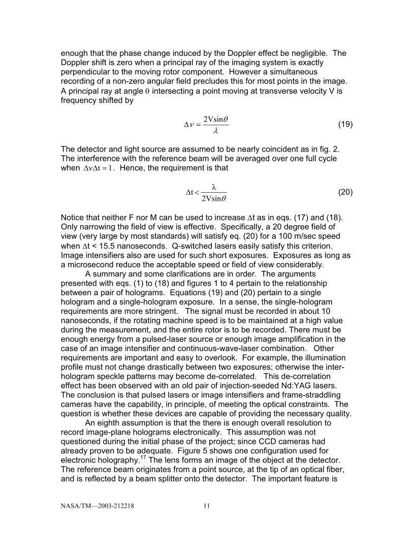
enough that the phase change induced by the Doppler effect be negligible. The Doppler shift is zero when a principal ray of the imaging system is exactly perpendicular to the moving rotor component. However a simultaneous recording of a non-zero angular field precludes this for most points in the image. A principal ray at angle θ intersecting a point moving at transverse velocity V is frequency shifted by

λ

θν 2Vsin=∆ (19)

The detector and light source are assumed to be nearly coincident as in fig. 2. The interference with the reference beam will be averaged over one full cycle when 1t =∆ν∆ . Hence, the requirement is that

θ2Vsin

λ t <∆ (20)

Notice that neither F nor M can be used to increase ∆t as in eqs. (17) and (18). Only narrowing the field of view is effective. Specifically, a 20 degree field of view (very large by most standards) will satisfy eq. (20) for a 100 m/sec speed when ∆t < 15.5 nanoseconds. Q-switched lasers easily satisfy this criterion. Image intensifiers also are used for such short exposures. Exposures as long as a microsecond reduce the acceptable speed or field of view considerably. A summary and some clarifications are in order. The arguments presented with eqs. (1) to (18) and figures 1 to 4 pertain to the relationship between a pair of holograms. Equations (19) and (20) pertain to a single hologram and a single-hologram exposure. In a sense, the single-hologram requirements are more stringent. The signal must be recorded in about 10 nanoseconds, if the rotating machine speed is to be maintained at a high value during the measurement, and the entire rotor is to be recorded. There must be enough energy from a pulsed-laser source or enough image amplification in the case of an image intensifier and continuous-wave-laser combination. Other requirements are important and easy to overlook. For example, the illumination profile must not change drastically between two exposures; otherwise the inter-hologram speckle patterns may become de-correlated. This de-correlation effect has been observed with an old pair of injection-seeded Nd:YAG lasers. The conclusion is that pulsed lasers or image intensifiers and frame-straddling cameras have the capability, in principle, of meeting the optical constraints. The question is whether these devices are capable of providing the necessary quality. An eighth assumption is that the there is enough overall resolution to record image-plane holograms electronically. This assumption was not questioned during the initial phase of the project; since CCD cameras had already proven to be adequate. Figure 5 shows one configuration used for electronic holography.17 The lens forms an image of the object at the detector. The reference beam originates from a point source, at the tip of an optical fiber, and is reflected by a beam splitter onto the detector. The important feature is

NASA/TM—2003-212218 12

that the reference source after reflection appears to be located at the center of the imaging lens, or relay lens if one is used. The limiting aperture and reference source are imaged near infinity, when a fiber is not used. Each principal ray from the imaged object coincides with a reference-beam ray, and the corresponding spatial frequency of the interference pattern is zero. This favorable circumstance of course does not apply to all the rays in a pencil from a point. Even at F/10, the extreme rays in the pencil require a resolution of 94/mm at 532 nm. An effective F of 40 or higher is required for recording the interference of all the rays. Rays that are not recorded simply contribute an intensity term that is subtracted in electronic holography as in eq. (11). The background light is undesirable, but a side benefit is that it is not a problem to vignette high frequency rays. The rays are not recorded anyway. A relay lens, without field lens, is often used in the object path.

Figure 5—One Setup for Electronic Holography.

A potentially serious problem occurs when it is necessary to relay the interference pattern itself. This requirement exists, for example, with an image intensifier. The relay process is characterized by a modulation transfer function (MTF) or optical transfer function (OTF) in case the different frequencies experience relative spatial shifts. The MTF is less than unity; declines with frequency; and multiplies the signal for each frequency during the relay process. The MTF of a CCD camera might be 75 percent for 300 TV lines along the horizontal direction. This resolution seems to be adequate for ordinary electronic

NASA/TM—2003-212218 13

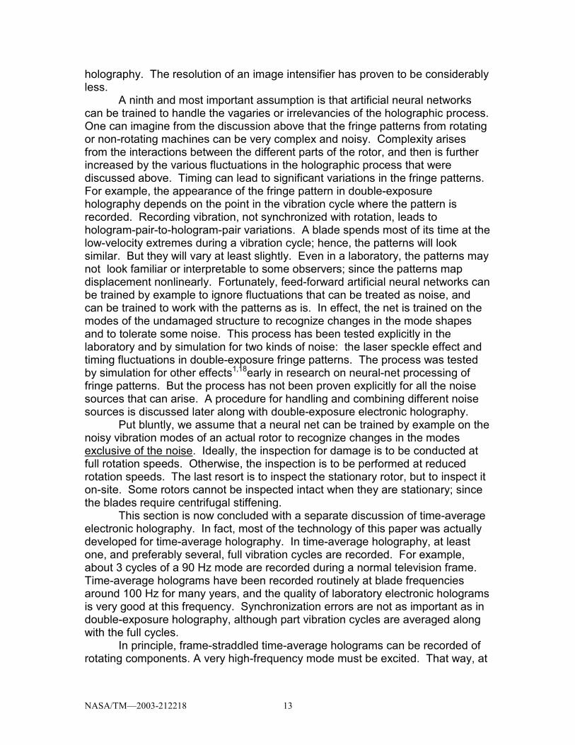
holography. The resolution of an image intensifier has proven to be considerably less. A ninth and most important assumption is that artificial neural networks can be trained to handle the vagaries or irrelevancies of the holographic process. One can imagine from the discussion above that the fringe patterns from rotating or non-rotating machines can be very complex and noisy. Complexity arises from the interactions between the different parts of the rotor, and then is further increased by the various fluctuations in the holographic process that were discussed above. Timing can lead to significant variations in the fringe patterns. For example, the appearance of the fringe pattern in double-exposure holography depends on the point in the vibration cycle where the pattern is recorded. Recording vibration, not synchronized with rotation, leads to hologram-pair-to-hologram-pair variations. A blade spends most of its time at the low-velocity extremes during a vibration cycle; hence, the patterns will look similar. But they will vary at least slightly. Even in a laboratory, the patterns may not look familiar or interpretable to some observers; since the patterns map displacement nonlinearly. Fortunately, feed-forward artificial neural networks can be trained by example to ignore fluctuations that can be treated as noise, and can be trained to work with the patterns as is. In effect, the net is trained on the modes of the undamaged structure to recognize changes in the mode shapes and to tolerate some noise. This process has been tested explicitly in the laboratory and by simulation for two kinds of noise: the laser speckle effect and timing fluctuations in double-exposure fringe patterns. The process was tested by simulation for other effects1,18early in research on neural-net processing of fringe patterns. But the process has not been proven explicitly for all the noise sources that can arise. A procedure for handling and combining different noise sources is discussed later along with double-exposure electronic holography. Put bluntly, we assume that a neural net can be trained by example on the noisy vibration modes of an actual rotor to recognize changes in the modes exclusive of the noise. Ideally, the inspection for damage is to be conducted at full rotation speeds. Otherwise, the inspection is to be performed at reduced rotation speeds. The last resort is to inspect the stationary rotor, but to inspect it on-site. Some rotors cannot be inspected intact when they are stationary; since the blades require centrifugal stiffening.

This section is now concluded with a separate discussion of time-average electronic holography. In fact, most of the technology of this paper was actually developed for time-average holography. In time-average holography, at least one, and preferably several, full vibration cycles are recorded. For example, about 3 cycles of a 90 Hz mode are recorded during a normal television frame. Time-average holograms have been recorded routinely at blade frequencies around 100 Hz for many years, and the quality of laboratory electronic holograms is very good at this frequency. Synchronization errors are not as important as in double-exposure holography, although part vibration cycles are averaged along with the full cycles.

In principle, frame-straddled time-average holograms can be recorded of rotating components. A very high-frequency mode must be excited. That way, at

NASA/TM—2003-212218 14

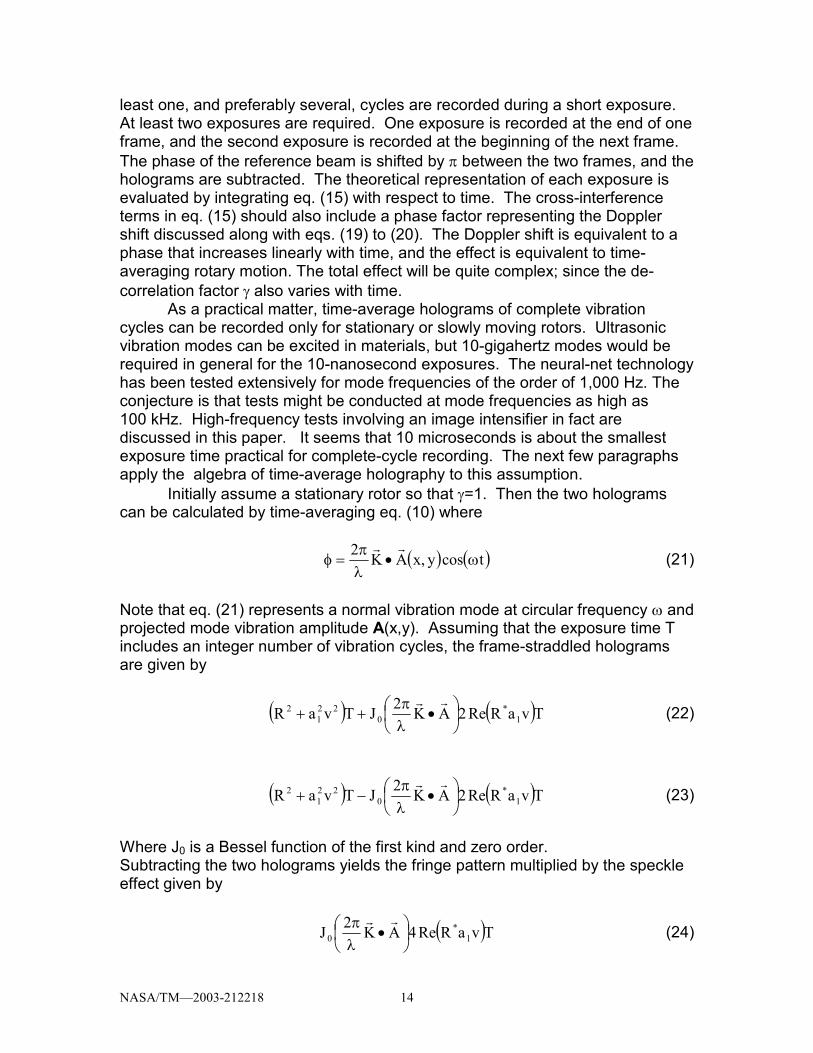
least one, and preferably several, cycles are recorded during a short exposure. At least two exposures are required. One exposure is recorded at the end of one frame, and the second exposure is recorded at the beginning of the next frame. The phase of the reference beam is shifted by π between the two frames, and the holograms are subtracted. The theoretical representation of each exposure is evaluated by integrating eq. (15) with respect to time. The cross-interference terms in eq. (15) should also include a phase factor representing the Doppler shift discussed along with eqs. (19) to (20). The Doppler shift is equivalent to a phase that increases linearly with time, and the effect is equivalent to time-averaging rotary motion. The total effect will be quite complex; since the de-correlation factor γ also varies with time.

As a practical matter, time-average holograms of complete vibration cycles can be recorded only for stationary or slowly moving rotors. Ultrasonic vibration modes can be excited in materials, but 10-gigahertz modes would be required in general for the 10-nanosecond exposures. The neural-net technology has been tested extensively for mode frequencies of the order of 1,000 Hz. The conjecture is that tests might be conducted at mode frequencies as high as 100 kHz. High-frequency tests involving an image intensifier in fact are discussed in this paper. It seems that 10 microseconds is about the smallest exposure time practical for complete-cycle recording. The next few paragraphs apply the algebra of time-average holography to this assumption.

Initially assume a stationary rotor so that γ=1. Then the two holograms can be calculated by time-averaging eq. (10) where

( ) ( )tcosyx,AK2ω•

λπ

=φrr

(21)

Note that eq. (21) represents a normal vibration mode at circular frequency ω and projected mode vibration amplitude A(x,y). Assuming that the exposure time T includes an integer number of vibration cycles, the frame-straddled holograms are given by

( ) ( )TvaRRe2AK2JTvaR 1*

022

12

•λπ

++rr

(22)

( ) ( )TvaRRe2AK2JTvaR 1*

022

12

•λπ

−+rr

(23)

Where J0 is a Bessel function of the first kind and zero order. Subtracting the two holograms yields the fringe pattern multiplied by the speckle effect given by

( )TvaRRe4AK2J 1*

0

•λπ rr

(24)

NASA/TM—2003-212218 15

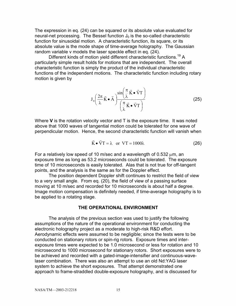
The expression in eq. (24) can be squared or its absolute value evaluated for neural-net processing. The Bessel function J0 is the so-called characteristic function for sinusoidal motion. A characteristic function, its square, or its absolute value is the mode shape of time-average holography. The Gaussian random variable v models the laser speckle effect in eq. (24). Different kinds of motion yield different characteristic functions.19 A particularly simple result holds for motions that are independent. The overall characteristic function is simply the product of the individual characteristic functions of the independent motions. The characteristic function including rotary motion is given by

•λπ

•λπ

•λπ

TVK

TVKsinAK2J0 rr

rr

rr (25)

Where V is the rotation velocity vector and T is the exposure time. It was noted above that 1000 waves of tangential motion could be tolerated for one wave of perpendicular motion. Hence, the second characteristic function will vanish when λ=λ=• 1000VTor TVK

rr (26)

For a relatively low speed of 10 m/sec and a wavelength of 0.532 µm, an exposure time as long as 53.2 microseconds could be tolerated. The exposure time of 10 microseconds is easily tolerated. Alas that is not true for off-tangent points, and the analysis is the same as for the Doppler effect. The position dependent Doppler shift continues to restrict the field of view to a very small angle. From eq. (20), the field of view of a passing surface moving at 10 m/sec and recorded for 10 microseconds is about half a degree. Image motion compensation is definitely needed, if time-average holography is to be applied to a rotating stage.

THE OPERATIONAL ENVIRONMENT

The analysis of the previous section was used to justify the following assumptions of the nature of the operational environment for conducting the electronic holography project as a moderate to high-risk R&D effort. Aerodynamic effects were assumed to be negligible; since the tests were to be conducted on stationary rotors or spin-rig rotors. Exposure times and inter-exposure times were expected to be 1.0 microsecond or less for rotation and 10 microsecond to 1000 microsecond for stationary rotors. Short exposures were to be achieved and recorded with a gated-image-intensifier and continuous-wave-laser combination. There was also an attempt to use an old Nd:YAG laser system to achieve the short exposures. That attempt demonstrated one approach to frame-straddled double-exposure holography, and is discussed for

NASA/TM—2003-212218 16

that reason. Images were to be relayed from the spin rig to the image plane using a fiber-optic bundle (fiberscope). The hologram or interference pattern was to be recorded directly by a CCD camera, or indirectly after amplification by the image intensifier. Changes in the recorded patterns were to be detected by artificial neural networks. The nets were to be trained with actual patterns so as to learn to ignore the vagaries of the holography process. Time-average as well as double-exposure patterns were to be used for the inspection of stationary rotors. The following concept of testing was to be employed. Vibration modes were to be excited in the rotor while rotating at full, reduced, or zero rotational speed. Holograms were to be recorded and the neural network trained from these holograms in the manner to be discussed later. The rotor was then to be subjected to a possibly damaging test. The test was to be interrupted periodically for a neural net inspection of recorded holograms for rotor changes or damage. The test ideally would be conducted at full speed, but possibly at reduced speed.

The remainder of this paper discusses the development and testing of the component technologies to implement this concept of testing. Both the successes and failures of the component technologies are presented. The first section summarizes the software and computer support.

SOFTWARE AND COMPUTER SUPPORT

The electronic holography and neural-net processing were performed entirely using Unix workstations.20 Programs were written in C-language and as Unix scripts. The workstation video21 was used to record the holograms. The video software was modified to incorporate neural-net processing as well as the hologram subtractions indicated by eqs. (11) and (16), and to visualize a variety of results. The software was used to assemble the holograms into training sets and to compute holograms from models to effect simulations. Neural nets were assembled, trained, tested, and converted to C-language code using a commercial software package.22 About 50 programs were created or modified in-house for this effort and the previous DDF project. Performing the holography and neural-net processing entirely with software limited both the rate and resolution possible. The setups achieved, or came close to achieving, the processing of 30 hologram pairs per second, but neural-net processing was limited to a few thousand large (re-binned) pixels. A future goal would be to adapt the neural-net features to personal computers and perhaps to exploit some hardware acceleration. Most PIV technology, including camera support, has been developed for the PC, and that technology is necessary to continue adapting electronic holography to rotating machines. The cameras and the lasers are critical, and are discussed briefly next.

NASA/TM—2003-212218 17

CAMERAS AND LASERS

Most of the work reported herein was accomplished with ordinary interlaced CCD television cameras. The inexpensively available technology of that sort is changing rapidly. At the time of writing of this paper, one could purchase for less than $1,000 still cameras with 250 microsecond electronic shutters. For comparison, it was challenging to use an expensive image intensifier to record electronic holograms in 50 microseconds to 400 microseconds during the R&D effort under discussion.

An ideal camera would meet the expectations of the operational environment using ordinary continuous-wave-laser illumination. The ideal camera would capture complete frames (as opposed to fields) with the inter-frame time less than a microsecond. Said cameras are readily available for PIV applications, where pulsed lasers are used to achieve the short exposure times. A manufacturer attempted, but failed, to provide such a camera for the project’s Unix workstation. Exposure times of a microsecond or less require a pulsed laser or an image intensifier. A lens-coupled image intensifier23 was acquired for the project, and its admittedly inadequate performance is discussed later. Several lasers were used for this project. Most frequently, holograms were recorded with the 514.5 nm line of an argon-ion laser. The argon-ion laser generates reasonably good results for object-to-reference path mismatches as large as 10 m. The ion-laser technology is becoming dated now that diode-pumped neodymium lasers are available. These lasers generate good results with object-to-reference path mismatches advertised as 100 m or larger and don’t require the cooling water of the ion lasers. The fiberscope holography system was designed to be used with a physically small diode-pumped Nd:YAG laser radiating 200 mw of 532 nm light. Most recently a 5 w neodymium vanadate laser was acquired for electronic holography. This laser also does not require water cooling. An external cavity diode laser was also evaluated, but its coherence length was not reliably large enough. An older pair of injection-seeded Q-switched Nd:YAG lasers was also available. The pulse width, and therefore exposure time, was about 5 nanoseconds, and the inter-exposure time could be reduced to about 1 microsecond. Each laser produced up to 500 millijoule of 532 nm light per pulse. The maximum tolerable object-to-reference path mismatch was about 1 m. An injection seeder forced both lasers to operate at the same frequency. A change in frequency introduces its own undesirable fringes. In principle, this laser could have satisfied many of the requirements of the operational environment, and its performance is discussed later. The laser system, in fact, lacked too many features of the modern PIV lasers and was large and unwieldy. A more serious defect was that the beam profiles of the two lasers differed significantly. Differences in the beam profiles result in speckle-pattern de-correlation as mentioned above. There is some concern that the beam profiles of a modern pair of PIV lasers might differ significantly. That performance can be tested in a manner to be discussed later.

NASA/TM—2003-212218 18

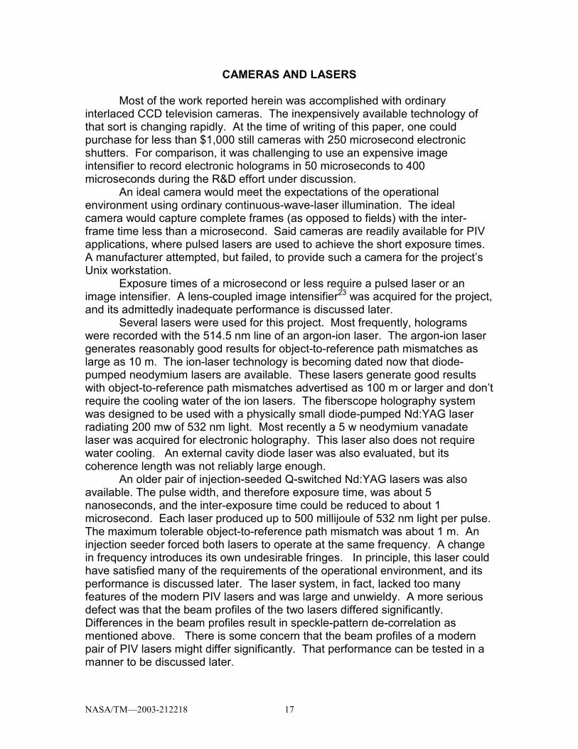
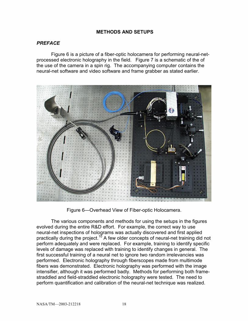
METHODS AND SETUPS PREFACE Figure 6 is a picture of a fiber-optic holocamera for performing neural-net- processed electronic holography in the field. Figure 7 is a schematic of the of the use of the camera in a spin rig. The accompanying computer contains the neural-net software and video software and frame grabber as stated earlier.

Figure 6—Overhead View of Fiber-optic Holocamera. The various components and methods for using the setups in the figures

evolved during the entire R&D effort. For example, the correct way to use neural-net inspections of holograms was actually discovered and first applied practically during the project.10 A few older concepts of neural-net training did not perform adequately and were replaced. For example, training to identify specific levels of damage was replaced with training to identify changes in general. The first successful training of a neural net to ignore two random irrelevancies was performed. Electronic holography through fiberscopes made from multimode fibers was demonstrated. Electronic holography was performed with the image intensifier, although it was performed badly. Methods for performing both frame-straddled and field-straddled electronic holography were tested. The need to perform quantification and calibration of the neural-net technique was realized.

NASA/TM—2003-212218 19

Figure 7—Schematic of Use of Fiber-Optic Holocamera in Spin Rig. The experimental setups and methods of the next sections are really

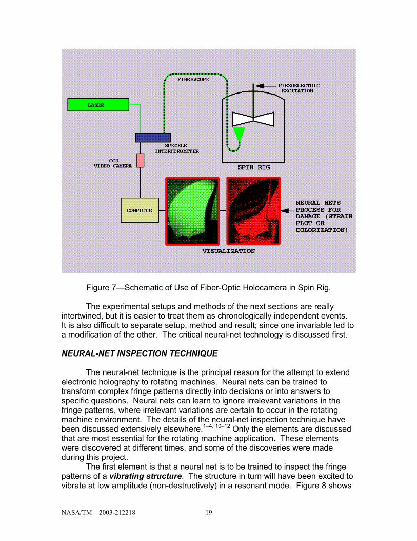
intertwined, but it is easier to treat them as chronologically independent events. It is also difficult to separate setup, method and result; since one invariable led to a modification of the other. The critical neural-net technology is discussed first. NEURAL-NET INSPECTION TECHNIQUE The neural-net technique is the principal reason for the attempt to extend electronic holography to rotating machines. Neural nets can be trained to transform complex fringe patterns directly into decisions or into answers to specific questions. Neural nets can learn to ignore irrelevant variations in the fringe patterns, where irrelevant variations are certain to occur in the rotating machine environment. The details of the neural-net inspection technique have been discussed extensively elsewhere.1–4, 10–12 Only the elements are discussed that are most essential for the rotating machine application. These elements were discovered at different times, and some of the discoveries were made during this project. The first element is that a neural net is to be trained to inspect the fringe patterns of a vibrating structure. The structure in turn will have been excited to vibrate at low amplitude (non-destructively) in a resonant mode. Figure 8 shows

NASA/TM—2003-212218 20

double- exposure and time-average fringe patterns of a particular vibration mode. The fringe patterns are called characteristic patterns because of an analogy with characteristic functions in statistics.

Figure 8—Time-Average and Double-Exposure Characteristic Patterns of a Mode From Electronic Holograms. An important second element is that a net is to be trained on the same

structure that will be inspected for structural changes and damage. This element is perhaps the most important neural-net-related finding of the R&D effort. Attempts have generally failed to train a neural net with the characteristic patterns of one structure to reliably detect changes in another manufactured copy of that structure. Several attempts to transfer training from the blades of an undamaged blisk to the blades of a damaged blisk were unsuccessful. Figure 9 actually shows a setup for training neural nets on the blisks. A holocamera for electronic holography is shown together with a blisk and a monitor (on the left) that displays some characteristic patterns of the blades. The resolution of training records into classes and unions is discussed later, and is based on the findings of the work discussed herein.

In a sense, the displayed blisk would be an ideal subject for a rotating machine test. The rotor can be inspected from the tip to the hub to generate the various speeds discussed in the section on technical justification. There were two blisks, and one had several blades that were cracked in an accident. A net trained with characteristic patterns from the undamaged blisk could not reliably detect the damaged blades in the damaged blisk. In fact, there

NASA/TM—2003-212218 21

was difficulty training a net with the undamaged blades of the damaged blisk to reliably detect the damaged blades in the same blisk. There were admittedly experimental difficulties. It was hard to isolate the vibration of a blade from entire-rotor effects. Another problem was that the sensitivity vector near the root was not favorable (see eq. (5)); since the blade twist made perpendicular viewing and illumination difficult. These experiments were conducted before a sensitivity enhancement technique called folding was discovered, and it was necessary to zoom onto the root with its unfavorable sensitivity vector to get results.

Figure 9—Setup Used to Record Training Sets for a Blisk. Eventually, the sensitivity vector problem was partially solved for

stationary rotors. A flexible fiberscope was inserted between the blades and was oriented perpendicular to the blade at the root. Illumination was admitted at an oblique angle, so that the sensitivity vector was still not optimum. The damage-detection capability improved nevertheless, where the net was trained to distinguish cracked blades from undamaged blades. Even then, cracks needed to be greater than 0.5 in. (1.27 cm), as shown by dye penetration, to be detected. The conclusion from this test and others was that blade-to-blade manufacturing variations even in a blisk affect the fringe patterns more than damage. The blisk inspections are discussed in more detail later.

A solution to be detailed below is to train the neural net on the fringe patterns of the specific undamaged structure of interest to detect small variations in that structure’s fringe patterns. The net will then respond to same-structure variations in the fringe patterns caused by damage or other changes.

The third element is to use the feed forward artificial neural-net architecture24 for structural inspections. The feed forward architecture is known for its noise immunity and can be trained to ignore irrelevant variations provided that enough examples of those variations are presented. The section on technical justification showed that the same blade in a rotating machine possibly

NASA/TM—2003-212218 22

would show a number of hologram-to-hologram variations not related to the structural integrity of the blade. The usefulness of neural nets depends entirely on being able to train the nets to ignore these variations. A large number of sample variations can be required to train the net. A conjecture is that neural nets can be trained to ignore multiple independent variations. This paper discusses in a later section on double-exposure holography the requirements for the simultaneously training of a net to ignore both the laser speckle effect and double-exposure timing fluctuations.

One of the conclusions from the blisk experiments was that there were not enough examples of manufacturing variations in the blades of a single blisk for training. The decision was to accomplish training only with the structure to be inspected in the manner to be discussed shortly. One untested conjecture was that training with probabilistic finite-element models25 that include realistic structural variations might replace training with multiple-blade examples.

The fourth element was to employ a degradable classification index DCI as the output of the feed-forward neural network. Figure 1012 shows schematically a feed-forward net, sometimes called a multi-layer perceptron for historical reasons. The architecture consists of processing nodes or neurons represented by circles. The nodes are arranged in layers. Most often information is transmitted in one direction only from left to right; hence, the net is called a feed-forward net. The nodes in one layer are connected to the nodes in the previous layer via weighted connections. These weighted connections are sometimes identified loosely with biological synapses. Typically the weighted inputs are summed and then transformed with a non-linear transfer function. Sigmoid and hyperbolic tangent functions are typically used for the transformation. The transformed output is then transmitted to the next layer of nodes for similar processing. The single output of a node is sometimes loosely identified with a biological axon. The most common training procedures are variations of the so-called back-propagation algorithm.

Figure 10—Diagram of Feed-Forward Neural Network. The important point for this paper again is that feed-forward nets easily

learn noisy data such as speckled fringe patterns. The pixel values of the fringe

NASA/TM—2003-212218 23

patterns are applied at the inputs as in Fig. 10. The second important point is that the output layer will contain two or three numbers called degradable classification indices DCI. Simply put one index is large for a pattern identical with one from the undamaged structure. Another index is large for any pattern that differs significantly from that pattern. The third index was originally used to identify patterns corresponding to particular kinds of damage, but is not used. Reliably the net distinguishes between unchanged and changed patterns. The third important point is that the DCI will change gradually as the pattern changes. Visualization can be accomplished by changing the color of the fringe pattern at a pre-defined value of the DCI.

The fifth element is to use finite-element-resolution sampling of the fringe patterns. Figure 11 shows normal and finite-element-resolution images of the fringe pattern of a normal mode of vibration. The finite-element-resolution input pattern contains only a few hundred to a few thousand pixels. Large pixels reduce resolution, but allow the software to process at high speed. Visualization rates of up to 30 frames per second have been demonstrated. The large pixel areas can also be sub-sampled randomly and repeatedly to generate un-correlated speckle patterns that are used to train the nets to ignore variations in speckle patterns. Training requirements that combine speckle and timing variations are discussed along with double-exposure holography in a later section.

Figure 11—(a) Characteristic Pattern From Silver-Halide Hologram; (b) Characteristic Pattern From Electronic Holograms; (c), (d) Finite-Element-Resolution Characteristic Patterns. The sixth and final element is to use an algorithmic training procedure.

The procedure is a major result of this R&D project. The procedure has been discussed elsewhere,10,12 but is listed again because of its importance. The procedure uses only holograms of the normal modes of vibration of the rotor components to be inspected. The procedure, developed during this R&D project, was applied to the inspection of an International Space Station ISS instrumentation cold plate.10,12 The procedure is listed for time-average holograms, for example, of a stationary rotor blade. Modifications for double-exposure holograms are discussed in another section. The key point to remember is that the net must specifically be trained to handle fluctuations not under control. The procedure is listed essentially as presented in reference 12.

NASA/TM—2003-212218 24

First, use electronic holography to identify about 5 vibration modes of the structure to be inspected.

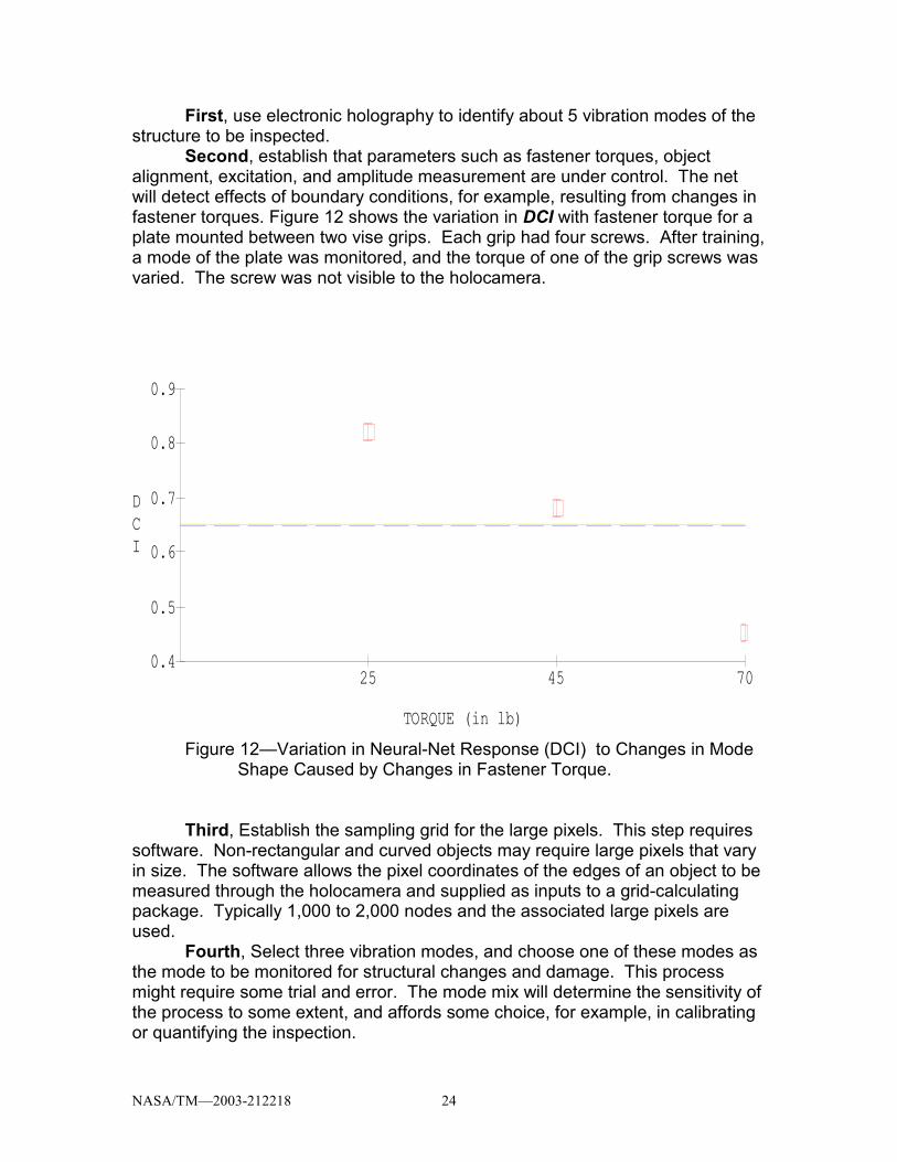
Second, establish that parameters such as fastener torques, object alignment, excitation, and amplitude measurement are under control. The net will detect effects of boundary conditions, for example, resulting from changes in fastener torques. Figure 12 shows the variation in DCI with fastener torque for a plate mounted between two vise grips. Each grip had four screws. After training, a mode of the plate was monitored, and the torque of one of the grip screws was varied. The screw was not visible to the holocamera.

Figure 12—Variation in Neural-Net Response (DCI) to Changes in Mode

Shape Caused by Changes in Fastener Torque. Third, Establish the sampling grid for the large pixels. This step requires

software. Non-rectangular and curved objects may require large pixels that vary in size. The software allows the pixel coordinates of the edges of an object to be measured through the holocamera and supplied as inputs to a grid-calculating package. Typically 1,000 to 2,000 nodes and the associated large pixels are used.

Fourth, Select three vibration modes, and choose one of these modes as the mode to be monitored for structural changes and damage. This process might require some trial and error. The mode mix will determine the sensitivity of the process to some extent, and affords some choice, for example, in calibrating or quantifying the inspection.

25 45 700.4

0.5

0.6

0.7

0.8

0.9

DCI

TORQUE (in lb)

NASA/TM—2003-212218 25

Fifth, Excite the vibration mode to be monitored for damage. The excitation level must be controlled. Fluctuations in the amplitude constitute a noise source. It may be possible to monitor a point on the object using a laser interferometer to assure that the vibration amplitude is controlled. An expert operator may also be able to set the amplitude adequately by viewing the characteristic pattern. Typically, the maximum excitation amplitude within the region being monitored will not exceed a wavelength. In double-exposure holography, amplitude changes between exposures will amount to wavelengths.

Sixth, Record the required number of speckle patterns. The rule is that un-correlated speckle patterns equal in number to 10 percent of the number of large pixels are required.1 Next append the output code for the mode to be monitored. As mentioned, two output nodes might be employed. The output code might be [1,0]. (The code [0.8, 0.2] is used for a sigmoid transfer function in a feed-forward net.) The first number is the DCI of the pattern to be monitored.

Seventh, Record the same number of un-correlated speckle patterns for the other two modes and for the zero-amplitude condition. Use another code for these patterns that places them in the same class. The output code might be [0,1] or [0.2,0.8] for a sigmoid transfer function. In effect, these patterns are examples of patterns that differ from the pattern-to-be-monitored. Changes in the mode shape of the pattern being monitored will then result in a decrease in its DCI and an increase in the other DCI as generated by the trained net.

Eighth, Construct a feed-forward net with 6 hidden-layer nodes,12 and train the net to an RMS error of 0.01 or less. The 6 hidden layers support 2 classes12 (undamaged structure and changed structure). There is a general discussion of training classes in a latter section on double-exposures. The RMS error is computed from the squares of the differences between the training outputs and measured outputs for all training records.

Ninth, Test the net for sensitivity. This step was still being developed at the time of writing of the paper, and is part of a follow-on R&D project. Ideally, the net is calibrated or at least quantified to be consistent with certain structural test criteria. One NASA approach is to make the neural-net test consistent with NASA vibration handbook standards. In the absences of calibration or quantification, simple judgment may be the only alternative. For example, light point loads can be applied at critical locations to test the neural net response, or fastener torques can be varied. These approaches are being investigated at the time of writing of this paper.

Tenth, Change the vibration-mode mix, if the sensitivity is not correct, and repeat the above steps. The vibration-mode-to-be-monitored is the most critical.

Eleventh, Establish criteria for interpreting the results of the test. For example, a change in the DCI from 0.8 to 0.7 might be declared to be an indicator of damage. At 0.7, an alarm can be triggered. One approach is to color the fringe pattern differently, when the DCI decreases below 0.7. A change of the fringe color from green to yellow or red can be used as an indicator. This viewpoint is decidedly an ANOVA viewpoint. For noisy data, a regression of the DCI against some test parameter such as time or the number of vibration cycles

NASA/TM—2003-212218 26

or the number of pressure cycles might be more appropriate. A trend can be established and its significance measured.

Experience has shown that these steps can be executed very quickly. The time required to record a training set; train the net; and link the net with other software is typically twenty minutes.

Another point not mentioned is that it is wise to avoid using the first vibration mode in the procedure. This mode is ubiquitous, and its best to let the experimentally measured training sets automatically incorporate its effects in both classes of patterns. This approach has been verified experimentally and with modeling. A major feature of early modeling work was the addition of a small amount of the first mode to the mode being monitored.

The neural-net inspection technique implies that training data are recorded experimentally. A neural-net training record consists of a fringe or characteristic pattern and a pair of DCI. In the laboratory, the inputs are developed from pairs of holograms as discussed previously. The holograms require a pair of frames. An ordinary TV camera divides each frame into two fields. In effect, four time-average holograms are recorded. Alternate frames are phase shifted by π, and corresponding field pairs are subtracted to yield fully interlaced characteristic patterns. The assumption, of course, is that the motion is entirely vibratory. Exposures occur in two fields during a frame time of a thirtieth of a second. Double-pulse holograms, where exposures might be as little as 5 nanoseconds, require a different viewpoint.

In any case, there is a question about how the data is to be prepared for the feed-forward net. The most straightforward approach is to scale the pixels between 0 and 1. The darkest pixel is 0 and the brightest pixel is 1. Another approach called a min-max table stretches the data for each pixel individually, from all the training records, between 0 and 1. A particular pixel will see both bright and dark speckles during a training session. Some pixels will be darker on average than others depending whether they are located at a fringe minimum or maximum. But dark pixels on average will be stretched between 0 and 1 along with bright pixels on average. A min-max table insures that each pixel uses the full input range of the neural network. A much better technique is available called folding. Folding was discovered during this R&D project and is a major accomplishment of that project. In any case, data acquisition and preparation are discussed next. DATA ACQUISITION, PREPARATION AND CONDITIONING The rotor or rotor component to be inspected for damage or changes must be used to prepare the training set as already stated. But the neural net really is being sensitized to detect changes in the entire electronic-holography detection process as well as the rotor. Hence it is important that the training set reflect all the elements of variation that are expected during data acquisition, preparation and conditioning. A few of these elements have been investigated systematically at this stage including the laser speckle effect and the combination of the speckle effect and double-exposure timing fluctuations. At times, it is

NASA/TM—2003-212218 27

difficult to isolate the important factors. A systematic classification approach is discussed in connection with double-exposures. Electronic holography is simple only in principle even in a laboratory. The structure’s surface may be painted or otherwise treated to yield a highly diffuse reflectivity. It may be inconvenient or impossible to use optimum surface preparation in a test facility. The phase and intensity profiles of the rotor illumination can fluctuate. Exposure-to-exposure variations are always possible with a pulsed laser. Optical path variations occur in the optics and atmosphere even in a laboratory and impose intensity and phase variations on both the object and reference beams. These variations are readily observed by viewing the characteristic pattern in time average holography without a phase shift. In principle, the subtraction, without a phase shift of π, should yield a completely dark image. In fact, the characteristic pattern and rotor image are observed to pop in and out at random as other factors introduce phase and intensity fluctuations. The intentional phase-shift process produces random fluctuations. The process was accomplished with an electro-optic phase modulator, and that approach introduced pattern-to-pattern fluctuations in the phase, the phase-profile, the intensity and perhaps the polarization. Subtraction therefore is not exact, and at least various fractions of the first term of eq. (22) remain and corrupt the characteristic pattern. The major effect is a contrast fluctuation, and nets have proven to be reasonably immune to contrast fluctuations. Shot-to-shot phase-profile fluctuations are potentially more damaging. A more reliable approach, not used for the results reported herein, is to shift the phase of the reference beam with a piezo-electric-stepped mirror. In principle, however, the electro-optic phase modulator can be switched more rapidly than a mirror, and that feature was expected to be required for nanosecond inter-exposure times. There has been little effort to improve the engineering of the above setup. The judgment now is that it is preferable to expend resources adapting the neural-net technique to commercial systems based on PCs rather than Unix workstations. The PCs have been adapted to use the PIV technology; whereas there is little new effort to adapt Unix workstations. The remainder of this section discusses the attention directed to the effective use of the camera-workstation combination. The camera as stated was an interlaced CCD camera intended for closed circuit television. Hence, a single-frame hologram really consists of two holograms captured in successive fields, each field lasting about 1/60 second. A vendor was unable to deliver the true frame camera originally intended for the project. The interlaced camera is really an artifact of television practice and is a nuisance for the work to be discussed. The images from the CCD camera were grabbed at the analog input of the workstation’s frame grabber. The camera records 640x480 pixels in two fields. Real-time (30 frame-per-second) visualization of time-average characteristic patterns requires the subtraction of successive frames. The software has proven to be a bit too slow to handle the subtraction of the entire frame at the full rate; hence real-time visualizations have been accomplished by subtracting hologram pairs corresponding to every other

NASA/TM—2003-212218 28

TV line or less. The absolute value of the difference is used for visualization on the computer monitor’s screen. Averaging of characteristic patterns can improve the visualization and is absolutely essential when using the noisy image intensifier. Figure 13 shows frames consisting of averages of 1, 100 and 1000 characteristic patterns from poor quality fiberscope holograms. Averaging improves the contrast of the characteristic pattern with respect to residuals of the first terms in eq. (22) or eq. (23) as well as electrical noise.

Figure 13—Averages of 1, 100 and 1000 Characteristic Patterns from Fiberscope Holograms. The neural net, as stated, processes only a few hundred to a few thousand pixels. To begin, the projected image of the structure is subdivided into

NASA/TM—2003-212218 29

a grid of what are called large pixels. The grid is generated automatically from measurements of the monitor image of the structure scaled in camera pixels. The grid generating procedure was actually developed for fan blades that are twisted and vertically oriented. The projected images of said blades tend to decrease in size from tip to root. The number of chord-wise pixels is held constant for each horizontal line; hence the blade is actually divided into trapezoidal regions in proceeding from root to tip. After choosing the number of large pixels, the left-edge offset and width of the projected image are measured at each vertical station. Each large pixel contains an array of camera pixels. The large pixel values are recorded in a somewhat non-conventional manner. The camera pixels are not rebinned or averaged. Instead a camera pixel is selected at random from within the large pixel region and subtracted from the corresponding pixel in the next hologram. Absolute values of the differences are stored. One pair from each large pixel region then generates the required number of inputs for the neural network. This process is repeated at different randomly chosen locations for successive holograms until enough training records are generated. Unfolded data are normalized in the range 0 to 1, and the appropriate DCI is appended to generate a training record. It is tempting to record only one pair of holograms and to generate the training records by sub-sampling within a single full-resolution characteristic pattern. But that process does not include elements of variation such as electrical noise. Selecting random locations within the large pixel assures de-correlated speckle patterns. The speckle patterns in a laboratory do not change fast enough to assure de-correlation, although there is some variation. Software controls the automatic recording and assembly of the large-pixel training records into a so-called training set. A test set of records can also be recorded.

The data handling process discussed so far is rational for human visualization using television or computer graphics. The training sets constructed from the raw data often are adequate. But early simulations with finite element models showed that the neural nets were not sensitive enough to detect the cracks generated with those models. It was necessary to use a crack amplification procedure by amplifying the effect of the crack on the vibration-displacement distribution 10 to 100 times, before the neural nets could be trained to detect the model generated cracks.1–4 Crack-detection sensitivity could be increased by zooming in on the affected region of the blade; thereby using more pixels and neural-net inputs from the affected region. But, it turned out that preparing data to suit human vision was not the most effective way.

The feed-forward net performs best when each input node sees data that covers the full input range. An input node at a dark fringe will not satisfy this requirement. One normalization approach called a min-max table stretches or distorts the data at each node to cover the full input range (0 to 1). This position- varying normalization procedure may increase the learning ability of a net for a particular training set, but the data are often over-fitted. That is, a slight variation in a pattern from a test set might result in a completely wrong response from the net. The net no longer generalizes. A much better procedure called folding was discovered during the rotating-machine project.

NASA/TM—2003-212218 30

Folding uses an intensity-dependent transformation of the data rather than a position or node-dependent transformation. The data are subdivided into different intensity ranges, and each range is stretched into the full input range of the neural network. The process begins with signed characteristic pattern such as given by eq. (24). Figure 14 shows the transformation for one and three folds. Note that taking the absolute value of characteristic patterns such as given by eq. (24) is equivalent to inserting one fold. Figure 15 shows the improvement in training and test errors as a function of the number of folds for a finite-element model of a particular blade having cracked and undamaged versions. Folding results in a displacement-change detection-sensitivity of better than 10 nanometers. Folding allows the finite-element-model generated cracks to be detected without amplification and, in fact, with de-amplification.11–12

One Fold

Three Folds Figure 14—Folding Transformation for Signed Characteristic Patterns and for One and Three Folds.

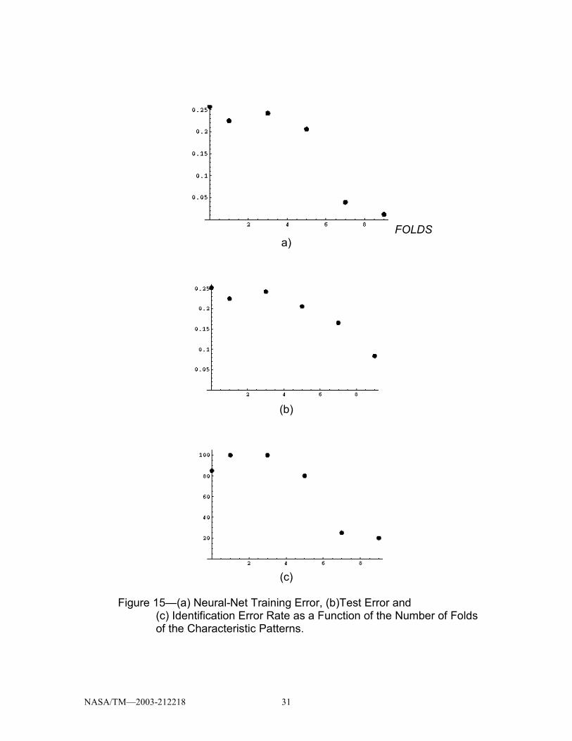
NASA/TM—2003-212218 31

FOLDS a)

(b)

(c)

Figure 15—(a) Neural-Net Training Error, (b)Test Error and (c) Identification Error Rate as a Function of the Number of Folds of the Characteristic Patterns.

NASA/TM—2003-212218 32

The caveat is that the performance of a neural net improves as the number of folds increases only until the net learns the training set. Increasing the number of folds beyond that point does not improve performance. A net that learns from the old absolute values of the characteristic patterns is already performing adequately. Folded test data must be used when the net is trained with folded data. Calculating folded inputs increases the response time of the net and reduces the chances for a real-time (30 frame-per-second) response.

As stated, visualization can be improved by averaging characteristic patterns. Characteristic patterns or folded characteristic patterns are the inputs to the neural networks. Averaging the outputs of neural networks can improve decision making. Specifically, averaging can answer whether one state is significantly different from another. Figure 12 is based on a simultaneous comparison of the averaged responses of the neural net at the torque settings displayed. The comparison was made using a one-way ANOVA. One hundred outputs were averaged at each torque setting to generate the figure. The same trend could be established without averaging only by regression.

The final discussion in this section pertains to frame straddling for short-exposure electronic holograms. The pulsed-laser and image-intensifier holograms occupy this category. More exactly the discussion pertains to field straddling; since a true frame camera (without interlace) was not available. In field straddling, there is always speckle-pattern de-correlation; since points in adjacent TV lines are subtracted. Hence, γ in eq. (6) will always be less than unity; since the mutual shift of speckle patterns uI is always non-zero. The damaging effect can be decreased only by decreasing the diameter D of the aperture or by increasing the F number of the imaging system. Field straddling has been used successfully nevertheless, although the quality of field-straddled characteristic patterns is poorer. But field straddling is easy to use for adjusting the timing of two exposures. The objective is to record the exposures in adjacent fields of successive frames or in the even and odd fields of the same frame. A magnified image of the TV line-pattern can be examined fairly easily on the computer monitor for the same or adjacent frames. If successive frames display opposite fields, then the double exposure has successfully straddled the frames. By contrast, exposing a single set of lines in one frame means that both exposures occurred in that frame and in one of the fields. Examining the magnified image will indicate whether the even or odd field was exposed. Hence one can determine whether the start time of the first exposure is to be moved forward or backward. A double-exposure in one frame that exposes both fields has straddled the fields successfully. Field and frame-straddling times as short as 4 microseconds were proven for the inexpensive interlaced CCD cameras used for this project, where the source was a pair of Q-switched Nd:YAG lasers. Note that the state-of-the-art for PIV cameras is only about 10 times better than this.

There is little doubt from the arguments in the section on technical justification that short-exposure double-exposure electronic holography will be required, if the machine rotates. The equipment for performing this technique adequately was not available, but the requirements were developed for

NASA/TM—2003-212218 33

neural-net interpretation of double-exposure electronic holograms. The next section discusses these requirements. The next section also serves as a preliminary discussion of how to handle more than one random process in training a neural net. SHORT-EXPOSURE-DOUBLE-EXPOSURE-HOLOGRAMS AS AN EXAMPLE OF HOW TO HANDLE TWO INDEPENDENT RANDOM PROCESSES IN TRAINING NEURAL NETS The following way to handle multiple independent random processes is still conjectural, but this approach works for double-exposure holograms. The approach was tested by simulation using a finite-element model of undamaged and cracked cantilevers. The finite-element model was combined with models of electronic holography, the laser speckle effect and the fluctuating phases of the double-exposures in order to generate the training and test sets. Several concepts are important in combining both random and deterministic processes. Experimental double-exposure work is discussed in the section on high-speed holocameras. The first concept to be grasped is that of a principal class. A principal class consists of samples that differ only in one random variable, where that random variable potentially assumes a large number of values. Characteristic patterns that differ only in the laser speckle effect constitute a principal class. As stated in the discussion of the algorithmic training procedure, a feed-forward neural net will learn to handle the laser speckle effect, if it is trained with random speckle patterns equal in number to ten percent of the number of input pixels. The neural-net requires about three hidden-layer nodes for each principal class. The second concept to be grasped is that of an effective principal class. An effective principal class reflects experimental reality. It contains random fluctuations that do not significantly change the response of the neural network. For example, an experimentally measured set of training records might purport to show a mode at a single vibration amplitude, but with varying speckle effect. The actual training set might be affected by various fluctuations in the optical train such as air currents and random variations of the phase modulator. The vibration amplitude might fluctuate slightly. Speckle-pattern correlation might fluctuate. Another mode might be excited at a low level. But the essential assumption is that the experimentally recorded class remains effective for training the net to ignore the laser speckle effect. The net may indeed develop some immunity to the other effects by their appearing in the training set, but there is no way to quantify that immunity. The third concept to be grasped is that of a class transition. The transition might be deterministic or random. A deterministic class transition might consist of a change in the vibration mode shape caused by damage. The objective is that the net flag that deterministic class transition. The net, by contrast, is to be trained to ignore a random class transition. The fourth concept to be grasped is that of a class union. A class union is a combination of classes that are trained to generate the same neural-net

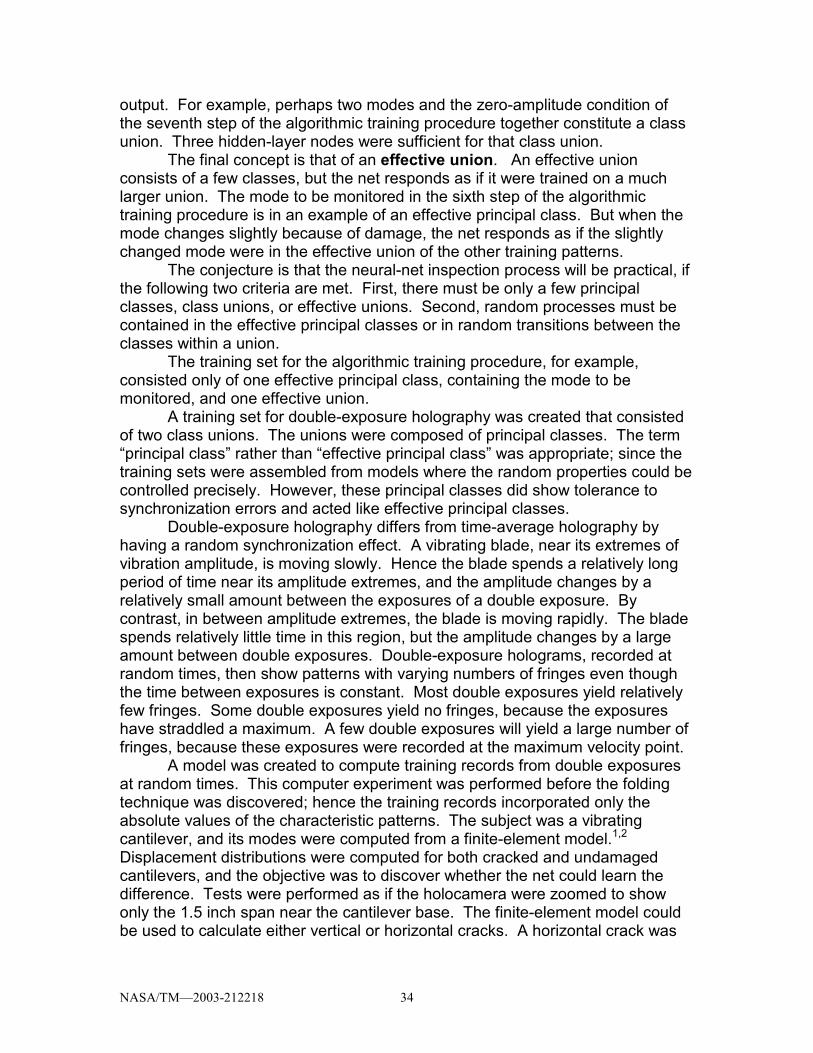
NASA/TM—2003-212218 34

output. For example, perhaps two modes and the zero-amplitude condition of the seventh step of the algorithmic training procedure together constitute a class union. Three hidden-layer nodes were sufficient for that class union. The final concept is that of an effective union. An effective union consists of a few classes, but the net responds as if it were trained on a much larger union. The mode to be monitored in the sixth step of the algorithmic training procedure is in an example of an effective principal class. But when the mode changes slightly because of damage, the net responds as if the slightly changed mode were in the effective union of the other training patterns. The conjecture is that the neural-net inspection process will be practical, if the following two criteria are met. First, there must be only a few principal classes, class unions, or effective unions. Second, random processes must be contained in the effective principal classes or in random transitions between the classes within a union. The training set for the algorithmic training procedure, for example, consisted only of one effective principal class, containing the mode to be monitored, and one effective union. A training set for double-exposure holography was created that consisted of two class unions. The unions were composed of principal classes. The term “principal class” rather than “effective principal class” was appropriate; since the training sets were assembled from models where the random properties could be controlled precisely. However, these principal classes did show tolerance to synchronization errors and acted like effective principal classes. Double-exposure holography differs from time-average holography by having a random synchronization effect. A vibrating blade, near its extremes of vibration amplitude, is moving slowly. Hence the blade spends a relatively long period of time near its amplitude extremes, and the amplitude changes by a relatively small amount between the exposures of a double exposure. By contrast, in between amplitude extremes, the blade is moving rapidly. The blade spends relatively little time in this region, but the amplitude changes by a large amount between double exposures. Double-exposure holograms, recorded at random times, then show patterns with varying numbers of fringes even though the time between exposures is constant. Most double exposures yield relatively few fringes. Some double exposures yield no fringes, because the exposures have straddled a maximum. A few double exposures will yield a large number of fringes, because these exposures were recorded at the maximum velocity point. A model was created to compute training records from double exposures at random times. This computer experiment was performed before the folding technique was discovered; hence the training records incorporated only the absolute values of the characteristic patterns. The subject was a vibrating cantilever, and its modes were computed from a finite-element model.1,2 Displacement distributions were computed for both cracked and undamaged cantilevers, and the objective was to discover whether the net could learn the difference. Tests were performed as if the holocamera were zoomed to show only the 1.5 inch span near the cantilever base. The finite-element model could be used to calculate either vertical or horizontal cracks. A horizontal crack was

NASA/TM—2003-212218 35

selected near the base of the cantilever. It was necessary to amplify the crack effect 10 times, before a net could be trained to detect the crack from either time-average or double-exposure holography. Folding should eliminate this need. The maximum amplitude of vibration at the blade tip was eventually selected to be 64 wavelengths of light (about 32 µm). The frequency of the mode was 91 Hz. The modes were sub sampled at a finite-element resolution of 21X43 nodes. The initial computer experiment was to assemble a training set from randomly phased double exposures. Contrary to the class model that subsequently proved essential, both the speckle effect and the double-hologram phase were varied at random. This process would be the most realistic experimentally in a rotating machine environment. Both the synchronization and the speckle patterns would be expected to vary in that environment. The performance was very poor for this kind of training. The neural nets successfully learned the training sets composed of patterns for the undamaged and cracked blades as well as the speckle patterns of a non-vibrating blade. But the nets did not learned to generalize, and they responded incorrectly to speckle patterns not contained in the training sets. In effect, an adequate union could not be assembled in this fashion. Not enough speckle samples were recorded for the relatively improbable rapid-motion double-holograms. The solution to this problem was to record the training sets with synchronization. Principal classes were created for each synchronization point and for the cracked and undamaged blades. Experimentally, synchronization probably would require that the training sets be assembled from a non-rotating stage, and it would be hard to handle significant centrifugal stiffening. Other effects such as de-correlation would not show up. These complications were not modeled in arriving at the following results. The following results and conclusions required a large number of computer experiments, but only the essential findings are stated. The time between exposures was 1000 microseconds. This time is about a tenth of a vibration period. A separate experiment showed that a net would respond correctly when the phase differed by π/12 from the synchronization point. The decision then was to divide the phase interval [0, π] into 5 start points. This choice allows phases to vary by as much as π/10 from the start point. The effect is mirrored in the interval [π, 2π]; hence separate starts in this interval were not required. The start points of the phase of the vibrating blade were then 0, π/5, 2π/5, 3π/5, 4π/5. Note that the start points preclude straddling the vibration maximum. Five principal classes of 100 speckle patterns each were assembled for the undamaged blade, and five principal classes of 100 speckle patterns each were assembled for the cracked blade. Hence there where 10 principal classes. The classes for the undamaged blade were assembled into an effective union. The classes for the cracked blade were also assembled into a second effective union. The training outputs for all the training records of an effective union are the same. Learning was very good. The RMS error was no more than about 0.02 for each principal class tested separately. The nets were then tested with different uncorrelated speckle patterns and randomly generated starting phases.

NASA/TM—2003-212218 36

However, pulses that straddled a displacement maximum were precluded. The training output was [0.8, 0.2] for one union and [0.2, 0.8] for the other. A DCI of 0.6 or higher was considered to be a positive identification. The minimum correct DCI was in fact 0.664. The rate of correct responses was 90 percent for 20 test patterns. Hence, the net learned to respond correctly to double-exposure patterns with random speckle patterns and random phase. The performance with 6 hidden-layer nodes, corresponding to 2 unions was good. But the response was actually slightly better for a net with two hidden layers. In fact, this simulation represented a rare case in the author’s experience where two hidden layers outperformed one hidden layer. The first hidden layer contained 9 nodes and the second hidden layer contained 6 nodes. The results and conclusions concerning the double-exposures are quite preliminary. The computer experiments were performed before discovery of the folding technique. But the need to assemble a training set with synchronization must be considered a drawback in performing rotating machine holography. The training set cannot be assembled from the state in which the rotor is to be tested. Perhaps the most important practical outcomes of this work are the rules for systematizing and evaluating training sets in terms of principal classes, effective principal classes, class transitions, class unions and effective unions. The fact that entire unions can be learned by adding only a few hidden-layer nodes to the net is significant. The results and conclusions, as mentioned, did not include any rotation effects. Test files were computed subsequently to include random rigid-body motion as well as vibration. These new test files, however, did not include de-correlation. The net that was trained without the rigid-body motion performed adequately when maximum rigid-body effects were about 10 percent of the vibratory effect. Remember that any motion affects the arguments of the characteristic functions depending on the sensitivity vector. Actual tangential motion can be considerably larger than vibratory motion for the same effect. The potential for successful rotating-machine holography, at this stage, depends critically on the performances of fiberscope electronic holography and image intensifiers. Fiberscope electronic holography is discussed next.

FIBERSCOPE ELECTRONIC HOLOGRAPHY

FUNDMENTALS OF FIBERSCOPE HOLOGRAPHY Electronic holography records focused-image holograms, and there is no fundamental reason why images relayed by a coherent fiber-optic bundle or fiberscope should not be useable. That conjecture is easy to confirm. Figure 16 shows characteristic patterns recorded directly and through a fiberscope. The fiberscope images of course are affected by the number of fibers in the bundle, and close examination of the fiberscope characteristic patterns show some deterioration as well as the graininess of the fiber array. But the number of optical channels greatly exceeds the number required by the neural networks in any case. Figures 6 and 7 show the fiber-optic electronic-holography setup

NASA/TM—2003-212218 37

used for the work reported herein. The intent was that the fiberscope be inserted through a vacuum seal into the spin rig. Simply put, a lens forms an image of the rotor or part of the rotor onto the input end of the fiber bundle. The bundle then transfers the image to the output end, where another lens relays the image to the CCD. The reference beam is superimposed on the image. It is, in fact, much more challenging to deliver enough laser power to illuminate the rotor or rotor component. The PIV profession uses articulated arms to route laser beams to the target. The decision for the work reported

Figure 16—Characteristic Patterns From Direct Images (left) and Fiberscope-Relayed Images (right). herein was to use fiber-optics to deliver the laser power. The flexibility, length, low-cost and ease of vacuum sealing of the fiber were factors in making this decision. It is a major challenge to prevent de-correlating fluctuations of illumination, when using fiber-optic delivery of the laser beam. Fluctuations cause speckle-pattern de-correlation as well as phase variations. Large-diameter optical fibers that handle relatively large amounts of power transmit beams through multiple paths or modes. The result is that a single TEM00 Gaussian laser beam inserted into a multi-mode fiber exits the fiber as multiple interfering beams. Figure 17 shows the complex interference effect of the exiting illumination. This phenomenon does not preclude effective electronic holography, and a viable characteristic pattern, recorded with the multi-mode illumination, is also shown in fig. 17. In fact, the average intensity of multi-mode illumination decreases more

NASA/TM—2003-212218 38

Figure 17—Illumination From a Multi-Mode Fiber and Characteristic Pattern Recorded With That Illumination. gradually than single-mode illumination. Non-nodal Bessel fringes can be displayed with higher contrast. Unfortunately, this pattern is extremely sensitive to fiber deflections and motion. A feather touch of the fiber disturbs the pattern and de-correlates the speckles. The multi-mode fiber is likely to be suitable only when excellent vibration isolation is available.

Single-mode polarization-preserving fibers are much more tolerant of disturbances and deliver a much cleaner beam as in fig. 18. But they are hard to align, and they effectively transport less power and couple it less efficiently. A practical power is a few hundred milliwatts. Nevertheless, the decision was to build the holocamera depicted in figs. 6 and 7 with a single-mode polarization preserving fiber for beam delivery. The fiber was to be used with a 200 mW diode-pumped frequency-doubled Nd:YAG laser It is desirable that the reference-beam fiber be cut to the same length as the combined lengths of the fiberscope and the illumination fiber for coherence-length matching. Some tests were conducted without the reference fiber, and it was necessary to have a long reference-beam path in air. Some of the new neodymium-ion lasers are sufficiently coherent that path matching is not as important. The reference-beam fiber is also a single-mode polarization-preserving fiber.

Figure 18—Illumination From Single-Mode Polarization-Preserving Fiber. Figure 19 shows modes recorded through a 20 ft fiberscope using single-

mode fiber-optic illumination. A neural-net was successfully trained using the algorithmic training procedure to recognize changes in the lyre mode excited at 2516 Hz.

NASA/TM—2003-212218 39

Figure 19—Modes Through 20 Foot Fiberscope.

A rotor consisting of a bladed disk (blisk) proved to be much more

challenging as an application of neural-net processed electronic holography. This rotor in fact exhibited some serious problems likely to be encountered in performing useful rotating-machine holography, even when the holographic and neural-net techniques work perfectly. The rotor test invites some serious thought about whether rotating machine holography is sufficiently practical. Nevertheless, that application showed a significant advantage of fiber-optic holography as discussed in the next section. NEURAL-NET PROCESSED CHARACTERISTIC PATTERNS OF A BLISK Figure 9 shows the holocamera and blisk combination as stated before. In fact, there were two blisks. Both contained eighteen blades, but one had been damaged by accidental rubbing during a previous test. The damaged blisk contained several cracked blades, where the cracks were observed using dye penetration. The cracks were located near the roots. The possibility existed, of course, that some blades had damage not made visible by dye penetration. Blade-to-blade manufacturing variations not related to damage complicate training. The early work on the blisks was done prior to discovery of the algorithmic training procedure and employed direct rather than fiber-optic holography. The tests were also conducted prior to discovery of the folding technique. Most of these tests involved zooming in on the root regions of the blades.

A very straightforward test was conducted after a number of other methods failed. The 18 blades of the damaged blisk were excited individually with both the exciter and blade carefully positioned, and training sets were recorded for each blade. In effect, eighteen effective principal classes were created. In addition, a class corresponding to the zero-amplitude condition was

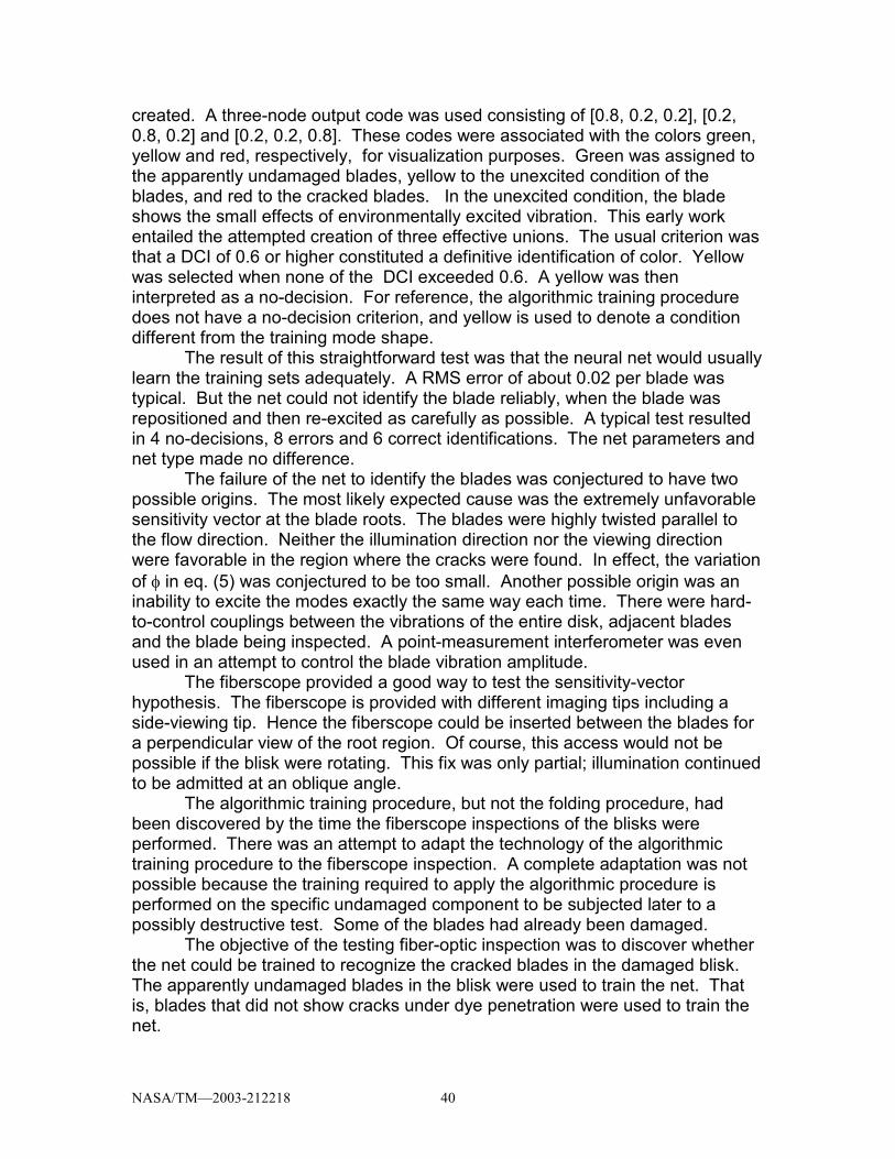
NASA/TM—2003-212218 40

created. A three-node output code was used consisting of [0.8, 0.2, 0.2], [0.2, 0.8, 0.2] and [0.2, 0.2, 0.8]. These codes were associated with the colors green, yellow and red, respectively, for visualization purposes. Green was assigned to the apparently undamaged blades, yellow to the unexcited condition of the blades, and red to the cracked blades. In the unexcited condition, the blade shows the small effects of environmentally excited vibration. This early work entailed the attempted creation of three effective unions. The usual criterion was that a DCI of 0.6 or higher constituted a definitive identification of color. Yellow was selected when none of the DCI exceeded 0.6. A yellow was then interpreted as a no-decision. For reference, the algorithmic training procedure does not have a no-decision criterion, and yellow is used to denote a condition different from the training mode shape. The result of this straightforward test was that the neural net would usually learn the training sets adequately. A RMS error of about 0.02 per blade was typical. But the net could not identify the blade reliably, when the blade was repositioned and then re-excited as carefully as possible. A typical test resulted in 4 no-decisions, 8 errors and 6 correct identifications. The net parameters and net type made no difference. The failure of the net to identify the blades was conjectured to have two possible origins. The most likely expected cause was the extremely unfavorable sensitivity vector at the blade roots. The blades were highly twisted parallel to the flow direction. Neither the illumination direction nor the viewing direction were favorable in the region where the cracks were found. In effect, the variation of φ in eq. (5) was conjectured to be too small. Another possible origin was an inability to excite the modes exactly the same way each time. There were hard-to-control couplings between the vibrations of the entire disk, adjacent blades and the blade being inspected. A point-measurement interferometer was even used in an attempt to control the blade vibration amplitude. The fiberscope provided a good way to test the sensitivity-vector hypothesis. The fiberscope is provided with different imaging tips including a side-viewing tip. Hence the fiberscope could be inserted between the blades for a perpendicular view of the root region. Of course, this access would not be possible if the blisk were rotating. This fix was only partial; illumination continued to be admitted at an oblique angle. The algorithmic training procedure, but not the folding procedure, had been discovered by the time the fiberscope inspections of the blisks were performed. There was an attempt to adapt the technology of the algorithmic training procedure to the fiberscope inspection. A complete adaptation was not possible because the training required to apply the algorithmic procedure is performed on the specific undamaged component to be subjected later to a possibly destructive test. Some of the blades had already been damaged. The objective of the testing fiber-optic inspection was to discover whether the net could be trained to recognize the cracked blades in the damaged blisk. The apparently undamaged blades in the blisk were used to train the net. That is, blades that did not show cracks under dye penetration were used to train the net.

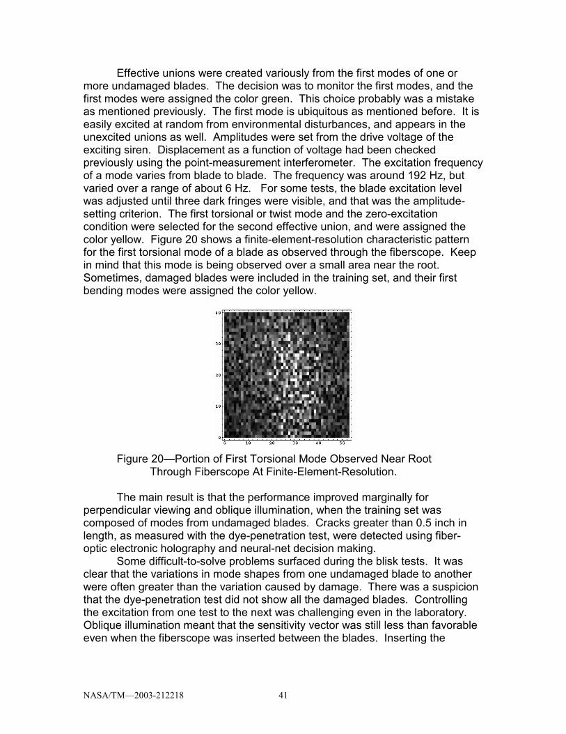
NASA/TM—2003-212218 41

Effective unions were created variously from the first modes of one or more undamaged blades. The decision was to monitor the first modes, and the first modes were assigned the color green. This choice probably was a mistake as mentioned previously. The first mode is ubiquitous as mentioned before. It is easily excited at random from environmental disturbances, and appears in the unexcited unions as well. Amplitudes were set from the drive voltage of the exciting siren. Displacement as a function of voltage had been checked previously using the point-measurement interferometer. The excitation frequency of a mode varies from blade to blade. The frequency was around 192 Hz, but varied over a range of about 6 Hz. For some tests, the blade excitation level was adjusted until three dark fringes were visible, and that was the amplitude-setting criterion. The first torsional or twist mode and the zero-excitation condition were selected for the second effective union, and were assigned the color yellow. Figure 20 shows a finite-element-resolution characteristic pattern for the first torsional mode of a blade as observed through the fiberscope. Keep in mind that this mode is being observed over a small area near the root. Sometimes, damaged blades were included in the training set, and their first bending modes were assigned the color yellow.

Figure 20—Portion of First Torsional Mode Observed Near Root Through Fiberscope At Finite-Element-Resolution. The main result is that the performance improved marginally for perpendicular viewing and oblique illumination, when the training set was composed of modes from undamaged blades. Cracks greater than 0.5 inch in length, as measured with the dye-penetration test, were detected using fiber-optic electronic holography and neural-net decision making. Some difficult-to-solve problems surfaced during the blisk tests. It was clear that the variations in mode shapes from one undamaged blade to another were often greater than the variation caused by damage. There was a suspicion that the dye-penetration test did not show all the damaged blades. Controlling the excitation from one test to the next was challenging even in the laboratory. Oblique illumination meant that the sensitivity vector was still less than favorable even when the fiberscope was inserted between the blades. Inserting the

NASA/TM—2003-212218 42

illuminating fiber between the blades in an attempt to improve the sensitivity vector resulted in an illuminated area of only about ¼ inch by ¼ inch. The conclusion was that the neural-net inspection technique requires that both training and testing be conducted on a single component. In effect, each component generates its own effective principal classes and unions. Another interpretation is that there were not enough manufacturing variations in a few blades to generate a statistically significant effective principal class based on manufacturing variations. This question might be answered best by using probabilistic finite-element modeling. The conclusion was that testing rotating blisks would have been a challenge, even had the holographic technology been adequate. But the high-speed detection and illumination hardware was far from adequate as discussed in the next section.

HIGH-SPEED HOLOCAMERAS MOST IMPORTANT PERFORMANCE CRITERION By far, the most important performance criterion for any hardware is that electronically-recorded speckle patterns, of an unchanging object, be correlated. This test, a necessary condition for good performance, is easy to perform for intensity alone. Then speckle patterns are recorded in adjacent frames or fields without a reference beam, and the Pearson’s or linear correlation coefficient is evaluated. The coefficient for a frame called F for first-frame and a frame called S for second-frame is given by

∑∑

∑−−

−=

i

2i

i

2i

iii

FS)SS()F(F

)S-)(SF(F ρ (27)

The index i labels corresponding pixels in adjacent frames (or fields). This coefficient is not to be confused with the correlation coefficient γ discussed in connection with equations (3) and (4). Equation (27) is a measure of incoherent correlation; whereas γ includes the effect of random phase. The ideal value of the linear correlation coefficient is unity for the combined illumination-and- recording system, but electrical noise, at least, precludes this. As a matter of experience, ρ < 0.7 is associated with unacceptably poor mode visualization, and ρ really should be close to unity. This result can be understood by noting that the root-mean-square difference in pixel energies between frames as a fraction of the root-mean-square fluctuation of the pixel energies about the mean in a frame is given by )-1(2 ρ . (28)

NASA/TM—2003-212218 43

Identical statistics have been assumed for the two frames. The fluctuation in energy difference is 77 percent of the fluctuation in the overall speckle effect by the time ρ = 0.7. Ironically, the opposite objective pertains to recording or computing un-correlated speckle patterns for training. Then a correlation coefficient near zero is desired. In early work, it was noted that |ρ| < 0.1 for model-generated speckle patterns containing a few hundred pixels. It was also found that |ρ| > 0.5 for experimental patterns with the same size. In effect, laboratory disturbances did not de-correlate the speckle patterns sufficiently to assemble independent training records and adequate training sets. The solution to this problem was to employ the large-pixel sub-sampling technique discussed previously. Then the experimental and model-generated correlation coefficients became comparable. The correlation coefficient has been measured at different times for a number of recording and illumination combinations. It must be kept in mind at all times that this coefficient is affected by averaging phenomena such as adjacent- pixel averaging effects. The linear correlation test is at best a necessary condition for adequate performance. CORRELATION COEFFICIENTS The best performance for the work reported herein was measured for the CCD-camera and continuous-wave-laser combinations. Corresponding pixels were used to calculate the correlation coefficient. An analog camera (640 x 480 pixels) with f/5 imaging, recording part of a cantilever illuminated with continuous-wave-laser illumination, yielded ρ > 0.97 for various frame comparisons. The correlations between exposures held for field-exposure times varying from 1/60 to 1/1000 second. Even cross correlations between frames recorded at different field exposure times were large. For example, ρ = 0.951 for a comparison between frames recorded at different field exposure times of 1/60 and 1/1000 second. The state-of-the-art in laboratory electronic holography imposes high standards on ρ. By contrast, a multiple-camera system did not perform well. The system consisted of eight cameras synchronized for high-speed motion analysis. Scenes recorded by different cameras did not correlate well. Correlation coefficients varied from about 0.5 at an exposure of 1/1000 second to 0.75 at an exposure of 1/100 second. The multiple-camera system proved to be totally inadequate. An image intensifier23 performed in the middle of the range between the CCD-camera and multiple-camera systems. The correlation coefficient was evaluated for an illuminated region of 299 x 307 pixels. Exposure times varied from 200 microseconds to 1000 microseconds. The individual exposures actually straddled the two fields of a frame, so the actual exposures per pixel ranged from 100 microsecond to 500 microseconds. The measured result was that ρ = 0.875. Note again that the fluctuation energy associated with the frame difference changes rapidly near ρ = 1 as given by eq. (28). The difference fluctuations between two image-intensifier frames is still large at 50 percent of

NASA/TM—2003-212218 44

the fluctuations in the speckle pattern of one frame for ρ = 0.87. For comparison, a CCD camera at ρ = 0.980 yields a fluctuation difference of 20 percent. It must be emphasized that keeping ρ close to unity is a necessary, but definitely not sufficient, condition for good performance. The linear correlation coefficient can be improved by averaging. Replacing a pixel with the average of its nearest neighbors will increase ρ. As an interesting exercise, an image processing routine was used to blur the image acquired from the image intensifier thereby increasing ρ to more than 0.99. The problem of course is that the resolution quickly becomes inadequate for electronic holography. As detailed in the next section, the performance of the image intensifier did not meet the needs of rotating machine holography, although it led to some interesting demonstrations of fringe-information processing. PERFORMANCE OF THE IMAGE INTENSIFIER FOR ELECTRONIC HOLOGRAPHY It should be noted that the image intensifier was recognized to be a-priori imperfect for the rotating machine application. The intensifier had relatively large optical channels that were lens-coupled (as opposed to fiber-coupled) to the analog cameras used for electronic holography. The analog cameras were not designed for the large pixels. As stated below, it was in fact necessary to magnify the holograms to compensate for the reduced resolution. Fringe magnification is an interesting, but not new, method for matching a spatial-frequency band to the capabilities of hardware. A fast output phosphor was selected with a decay time of 300 nanoseconds so that the intensifier would at least match the state-of-art inter-frame times of CCD cameras of around 200 nanoseconds. The early suspicion was that the image intensifier, continuous-wave-laser combination would eventually need to be replaced with a pulsed laser system, if work in rotating machine holography were to continue. The initial measurement showed that the sensitivity of the image intensifier was marginal for rotating machine holography. A full Watt of laser power was required to image a portion of a ruler when the gate time was 200 nanoseconds. Recall that exposure times of about 15 nanoseconds or less are required for rotating machine holography at full rotation speeds. Hence, at best, only 10 percent of the radius of the rotor could be recorded at full speed, and then in small sections. Observing the ruler required a gate time of 600 nanoseconds when a laser power of 200 mW was delivered through a fiber. In general, good results required gate times of many microseconds, thereby effectively eliminating applications to a rotating stage. The generation of useful holograms and characteristic patterns was tested using time-average holography. Modes with frequencies in excess of 10,000 Hz are required for time averaging with field times of 100 microseconds. Modes with frequencies greater than 2000 Hz are required at field times of 500 microseconds.

NASA/TM—2003-212218 45

At this point, it must be emphasized that the image intensifier is an interference-pattern transfer device. An image is formed of the interference pattern or hologram, and that image is then amplified. This process contrasts with that of the fiberscope. The fiberscope transfers an image of the object, and that image is then combined with a reference beam to form a hologram. The fiberscope will reduce the resolution of the image of the object, but not the resolution of the interference pattern; whereas the image intensifier will reduce the resolution of the interference pattern or hologram, itself. One conceptual analysis of this process begins by imagining calculating the Fourier transform of the hologram. Each component of the transform is then imagined to be multiplied by the OTF or optical transfer function of the overall intensifier and imaging system. Most analyses ignore the phase shift or position shift of each component and use only the magnitude of the OTF. The magnitude of the OTF is called the modulation transfer function or MTF. The MTF is always less than or equal to unity. For example, the MTF of a perfect simple lens is nearly linear, decreasing steadily from 1.0 at zero frequency to 0.0 at the cutoff frequency of the lens. The cutoff frequency is essentially the reciprocal of the resolution, where the resolution is given for example by eq. (1) with M = 1. It turns out that the MTF of the lens-coupled image intensifier decreases much more rapidly. Figure 21 shows schematically this effect. In effect, the overall gain for higher frequencies is reduced.

Figure 21—Diagram of Behavior of MTF of Intensifier When

Compared with Simple Lens. The general effect on characteristic patterns of a decrease in the resolution for detecting a hologram is shown in Figure 22. CCD-recorded holograms were used for this simulation rather than intensified holograms.

NASA/TM—2003-212218 46

Resolution was reduced through averaging neighboring pixels using a workstation-resident image processor. The first image was created at full resolution. Hologram resolutions for subsequent images differed roughly by factors of 2, 4 and 8 from full resolution. The performance of the image intensifier can be summarized with a few sentences. The intensifier amplified weakly the power associated with the spatial frequencies of importance in forming characteristic patterns (eqs. (11) or (16)). The intensifier unfortunately amplified lower-frequency interference effects very well. There were weak extraneous beams created in the reference-beam path, and these beams interfered with the reference beam. These low-frequency interferences were amplified dramatically and never subtracted out completely. Even the best results showed some residual low-spatial-frequency stripes. A small benefit was generated by the low-pass filtering of the high-frequency self-interference effects, such as would be produced by the second terms in eqs. (9) and (10).

Figure 22—Change in Appearance of Characteristic Pattern as Resolution of Holograms Decreases. In fact, it was necessary to magnify the holograms to match the useful band pass of the intensifier and generate any results The holograms were magnified, thereby reducing the frequency of the interference pattern to be passed through the intensifier. Keep in mind that the image of the object and the hologram itself coincide for the focused-image holograms used for electronic holography. Hence, magnifying the hologram also magnifies the image of the object, and reduces the portion of the image and hologram passing through the intensifier. A typical magnification factor was 6X. Hence, the information-carrying frequencies were reduced by a factor of six from the frequencies normally processed in CCD electronic holography. Without this magnification process, image-intensified holography could not be performed.

NASA/TM—2003-212218 47

Figure 23 shows a characteristic pattern obtained from intensified holograms of a blade. The holograms were first magnified 6X and then passed through the intensifier. The blade was illuminated with 10 mw for the holograms, and the exposure times were 16 milliseconds per field. The figure is an average of 30 characteristic patterns. Integration and averaging seemed to be required even for the magnified holograms. Figure 23 was processed for some haze removal. As mentioned, the stripes visible are associated with an interference effect with an extraneous beam in the reference-beam path.

Figure 23—Characteristic Pattern From Intensified Holograms. Figure 24 shows an average of 100 characteristic patterns from the intensifier, CCD-camera combination. Two fields were exposed in 30 milliseconds. Bessel fringes appear in addition to the nodal fringe. The low-frequency interference effect is still visible.

Figure 24—Average of 100 Characteristic Patterns Where Holograms Were Intensified.

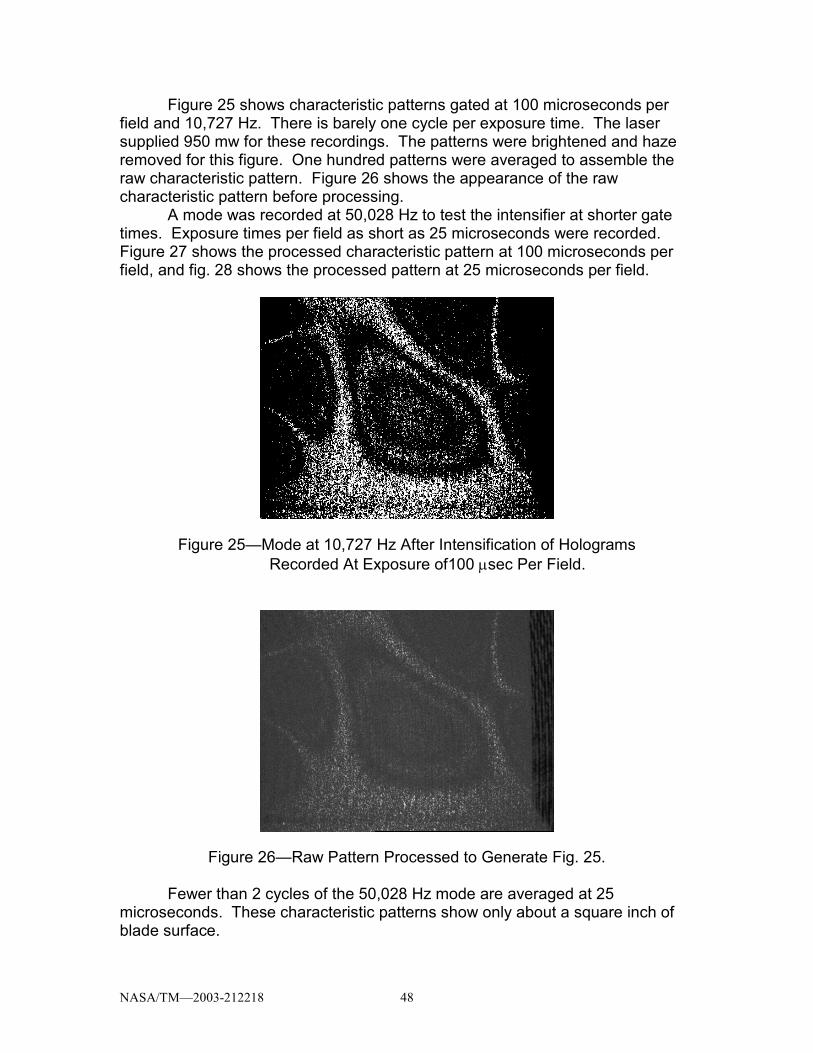
NASA/TM—2003-212218 48

Figure 25 shows characteristic patterns gated at 100 microseconds per field and 10,727 Hz. There is barely one cycle per exposure time. The laser supplied 950 mw for these recordings. The patterns were brightened and haze removed for this figure. One hundred patterns were averaged to assemble the raw characteristic pattern. Figure 26 shows the appearance of the raw characteristic pattern before processing. A mode was recorded at 50,028 Hz to test the intensifier at shorter gate times. Exposure times per field as short as 25 microseconds were recorded. Figure 27 shows the processed characteristic pattern at 100 microseconds per field, and fig. 28 shows the processed pattern at 25 microseconds per field.

Figure 25—Mode at 10,727 Hz After Intensification of Holograms Recorded At Exposure of100 µsec Per Field.

Figure 26—Raw Pattern Processed to Generate Fig. 25.

Fewer than 2 cycles of the 50,028 Hz mode are averaged at 25 microseconds. These characteristic patterns show only about a square inch of blade surface.

NASA/TM—2003-212218 49

Figure 27—Characteristic Pattern From Intensified Holograms At 50,028 Hz and Field Exposures of 100 µsec.

Figure 28—Mode at 50,028 Hz, But With Field Exposures of 25 µsec. These intensifier exposure times are at least two orders of magnitude greater than the exposure times required for a sensible evaluation of reduced-speed rotating machine holography. That assumes that we could even synchronize to integrate and average repeats of the characteristic patterns. As mentioned, an old pulsed laser was available, and its performance is discussed briefly next. PULSED LASER HOLOGRAMS There was a Q-switched, frequency-doubled Nd:YAG laser system available that in principle could meet the requirements of rotating stage holography. The system consisted of two lasers the were locked to the same frequency by a single injection seeder. The estimated coherence length of the lasers was about a meter. The lasers each had a pulse width of about

NASA/TM—2003-212218 50

5 nanoseconds; hence the Doppler-shift restriction of eq. (20) was easily met. The time separation between pulses could be reduced to about one microsecond or increased to about one millisecond. Hence, it should have been possible to satisfy equations (17) and (18) at various speeds and for a significant part of the rotor even at high speed. Each laser produced pulses of about 500 mJ at a wavelength of 532 nm. There were three problems with the laser technology. The laser system was quite dated (circa 1988) and somewhat large and unwieldy. The laser beam profiles were visually different and unmatched, thereby introducing significant speckle pattern de-correlation. Finally, Q-switched laser power is not well-suited to fiber-optic delivery. A periscope would have been required, together with its cost and vacuum sealing requirements. Another problem was that the cameras in use exposed the holograms in two fields. In frame-straddled double-exposure holography, one exposure would expose the second field of one frame and the other exposure would expose the first field of the second frame. A contractor was unable to deliver a camera that would expose all lines in a frame simultaneously and that could be operated from the Unix workstation. Such cameras are readily available for PCs. The combination of beam-profile-induced de-correlation and line-offset de-correlation proved to be too destructive. This problem was probably aggravated by the difficulty of balancing the intensities of the two beams whose profiles differed. A lack of balance prevents a complete subtraction of the first two terms of eq. (10) necessary for the result implied by eq. (11). Nevertheless, at least the consequence of frame-straddling in two different fields was easy to demonstrate. The demonstration employed magnified holograms as with the image intensifier. A blade mode was excited, and double- exposure holograms were recorded using only one of the two lasers. Hence, the repeatability of the beam profile could be assured. The laser firing rate and synchronization were adjusted either to record the two holograms in the same field in different frames or in opposite fields in different frames. The laser system operates at up to 10 pulses or double-pulses per second. Figure 29 shows a characteristic pattern calculated from the same field but in different frames. There is no line-offset in this case. The pattern is clear but grainy; since every other line is missing. Figure 30 shows a characteristic pattern calculated from opposite fields. The mode frequency was 1860 Hz. This situation would represents frame straddling when an ordinary television camera is employed. There is line-offset, and the fringe contrast is substantially degraded.

NASA/TM—2003-212218 51

Figure 29—Characteristic Pattern Using Nd:YAG Laser Where the Same Laser and Corresponding Fields in Adjacent Frames Were Used.

Figure 30—Characteristic Pattern Using Nd:YAG Laser Where the Same Laser and Opposite Fields in Adjacent Frames Were Used. Degradation was much more substantial when two lasers were used. The combination of a line shift, beam-profile-induced de-correlation, and unbalanced subtraction proved fatal for 1.0 millisecond pulse separations and modes at 200 Hz and 1860 Hz. Figure 31 shows the result at 200 Hz. Essentially no characteristic pattern is detectable.

NASA/TM—2003-212218 52

Figure 31—Characteristic Pattern Using Twin Nd:YAG Lasers and Opposite Fields in Adjacent Frames (Normal Frame Straddling).

SUMMARY AND DISCUSSION OF RESULTS

The procedures discovered for acquiring, organizing, conditioning, and applying neural-net training records constitute the major practical results of this work. These procedures are discussed in METHODS AND SETUPS, and did not exist before they were discovered during the rotating-machine-holography project. The procedures require careful preparations, and have been verified in the laboratory. But the fiber-optic holocamera enables the procedures for field applications as well. The successful algorithmic NDE procedure is essentially a detector of changes. The neural network, when correctly trained, will detect any changes in the characteristic pattern being monitored, except those changes that the net is specifically trained to ignore. A feed-forward neural network is used for these applications. The net most often contains one hidden layer and three hidden-layer nodes per principal class. The mode to be monitored resides in a principal class by itself that contains enough examples of the laser speckle effect for speckle-effect immunity and probably contains some other variations induced by the environment. All other modes, including changes in the mode-to-be-monitored, are contained in an effective union. The first vibration mode should be avoided for training; since it is excited too easily by environmental factors and is probably present as a background effect in all effective principal classes. The training-set acquisition procedure is essentially algorithmic and is executed with software. Training can be accomplished very rapidly. The approach to fiberscope electronic holography as discussed in FIBERSCOPE ELECTRONIC HOLOGRAPHY is the second major practical result of this work. Fiberscopes do not affect the resolution of the electronic holograms, but only the resolution of the focused image. Fiber-optic delivery of laser power for illumination of the object is challenging. Single-mode fibers can be used to deliver fairly large amounts of power. Multi-mode fibers can be used, but require careful vibration isolation. The fiberscope has the additional

NASA/TM—2003-212218 53

advantage that it can be oriented for a perpendicular view of difficult-to-access surfaces such as a blade surface near a root. Image-intensified holography was selected as the tool for the rotating-stage environment, but the final results turned out to be mainly of academic rather than practical interest. As discussed in HIGH-SPEED HOLOCAMERAS, the image intensifier that was tested lacked both the sensitivity and the resolution for the intended application. Minimum feasible exposure times were around one microsecond. Time-average holograms were recorded with exposure times as low as 25 microseconds. An exposure time of one microsecond is still about two orders of magnitude too large for practical rotation speeds as discussed in TECHNICAL JUSTIFICATION FOR ATTEMPTING ROTATING STAGE HOLOGRAPHY. The effective resolution element or optical-channel size of the intensifier was also large. An interesting procedure was used to compensate. The focused-image holograms were magnified about 6X to shift the useful energy into the spatial-frequency band that the intensifier could handle. Time-average holograms at frequencies greater than 50,000 Hz were then used to evaluate the process. The results were acceptable, but sometime 10 to 100 characteristic patterns were averaged to produce a good pattern. A practical criterion was proposed in HIGH-SPEED HOLOCAMERAS for specifying the a-priori performance of characteristic-pattern generators. The Pearson’s or linear correlation coefficient of adjacent object-beam patterns should be close to unity. A suggested value is at least 0.95. The coefficient should be measured at the full resolution specified for the hardware; since the correlation coefficient can be increased by spatial averaging and reducing resolution. The correlation coefficient for continuous-wave lasers and CCD cameras exceeds 0.97, and these components have been proven for electronic holography. The criterion represents a necessary, but not sufficient, condition and must be applied carefully. The Pearson’s correlation coefficient is not the same as the correlation coefficient associated with eq. (4) and other equations in TECHNICAL JUSTIFICATION FOR ATTEMPTING ROTATING STAGE HOLOGRAPHY. A pulsed laser system that does not meet the correlation-coefficient specification can be discarded immediately. Rotors can be difficult to inspect even with adequate holography systems and neural-net techniques. This result followed from a blisk inspection as discussed in FIBERSCOPE ELECTRONIC HOLOGRAPHY. The blisk was hard to vibrate in a controlled manner and afforded non-optimum sensitivity vectors such as discussed in connection with eq. (5) in TECHNICAL JUSTIFICATION FOR ATTEMPTING ROTATING STAGE HOLOGRAPHY. Perhaps the most valuable finding of the blisk inspection was the importance of training on precisely the component to be inspected. Another important finding from the blisk inspection was the usefulness of fiberscopes for optimizing the sensitivity vector.

NASA/TM—2003-212218 54

CONCLUSIONS AND CONCLUDING REMARKS

The major conclusions drawn from this work are that rotating-stage electronicholography requires modern Q-switched double-pulse lasers, and that the neuralnet processing method works well enough to be developed and exploited extensively. The shortcut involving image intensifiers unfortunately does not work well enough to be exploited. Beam delivery and recording for pulsed lasers can be accomplished with the hardware already developed for PIV. The Unix workstations should be replaced by PCs so that the best camera technology can be employed. Lasers and cameras should be evaluated initially in terms of their abilities to generate correlated pairs of frames. Full-frame cameras with short inter-frame times should be used so that corresponding lines and pixels can be subtracted and subtracted rapidly. Each component of the holocamera must operate flawlessly. Tolerating a train of components, each slightly degraded from optimum, leads to failure. In general, the available hardware for rotating-stage electronic holography is expensive, and performance is not guaranteed. A manufacturer of pulsed lasers was hesitant about meeting the simple correlation test discussed in this paper. Hence, rotating machine work of the kind discussed herein would have to be continued as high-risk R&D. The neural-net inspection method itself has developed substantially and usefully during this project. The recommendation is that the neural-net method be exploited and developed further. The neural-net method should be made consistent with existing NDE methods and calibrated or quantified. Field –inspection methods using electronic holography and neural nets should be tested initially in a non-rotating environment.

REFERENCES

1. A.J. Decker., E.B. Fite., O. Mehmed. and S.A. Thorp, “Processing speckle patterns with model trained neural networks,” Optical Technology in Fluid, Thermal, and Combustion Flow III, Proc. SPIE, vol. 3172, pp. 285–293, July 1997.

2. A.J. Decker., E.B. Fite., O. Mehmed. and S.A. Thorp, “Vibrational Analysis of Engine Components Using Neural-Net Processing and Electronic Holography,” Advanced Non-Intrusive Instrumentation for Propulsion Engines, AGARD–CP–598, pp. 33–1—33–6, May 1998.

3. A.J. Decker, E.B. Fite, S.A. Thorp, and O. Mehmed, “Comparison of computational-model and experimental-example trained neural networks for processing speckled fringe patterns,” International Conference on Optical Technology and Image Processing Fluid, Thermal, and Combustion Flow, Proceedings of VSJ–SPIE ’98, on compact disc in pdf, paper AB002, 1998.

NASA/TM—2003-212218 55

4. A.J. Decker, “Neural-Net Processing of Characteristic Patterns,” Topics on Nondestructive Evaluation Series, Automation, Miniature Robotics and Sensors for Nondestructive Evaluation and Testing, Yoseph Bar-Cohen, Technical Editor, vol. 4, chapter 7.1, The American Society for Nondestructive Testing, Inc., 2000.

5. K.A. Stetson, “The Use of an Image Derotator in Hologram Interferometry and Speckle Photography of Rotating Objects,” Experimental Mechanics 18, pp. 67–73, 1978.

6. C.M. Vest, Holographic Interferometry, p. 243 (See fig. 4.38 provided by K.A. Stetson), Wiley, New York, 1979.

7. C. Perez-Lopez, et. al., “Pulsed digital holographic interferometry for dynamic measurement of rotating objects with an optical derotator,” Applied Optics 40, pp. 5106–5110, 2001.

8. P. Gren, “Pulsed TV holography combined with digital speckle photography restores lost interference phase,” Applied Optics 40, pp. 2304–2309, 2001.

9. P. Gren, “Bending wave propagation in rotating objects measured by pulsed TV holography,” Applied Optics 41, pp. 7237–7240, 2002.

10. A.J. Decker, M.E. Melis, and K.E. Weiland, “Inspection of Space Station Cold Plate Using Visual and Automated Holographic Techniques,” NASA/TM—1999-209388, Aug. 1999.

11. A.J. Decker, “Training Data Optimized and Conditioned to Learn Characteristic Patterns of Vibrating Blisks and Fan Blades,” Research and Technology 2000, NASA/TM—2001-210605, pp. 63–64, 2000.

12. A.J. Decker, “Optimization of training sets for neural-net processing of characteristic patterns from vibrating solids,” Optical Diagnostics for Fluids, Solids, and Combustion, Proc. SPIE, vol. 4448, pp. 209–217, 2001.

13. M.P. Wernet, “Particle Displacement Tracking Applied to Air Flows,” NASA Technical Memorandum 104481, Prepared for Fourth International Conference on Laser Anemometry, Cleveland, Ohio, Aug. 5–9, 1991.

14. A.J. Decker, “Neural-Net Processed Characteristic Patterns for Measurement of Structural Integrity of Pressure Cycled Components,” NASA/TM—2001-210812 for Proceedings of JANNAF, 12th Nondestructive Evaluation Subcommittee, Cocoa Beach, Florida, 26–30 March 2001.

15. R. Dändliker, “Heterodyne Holographic Interferometry,” Progress in Optics, vol. 14, E. Wolf, ed., pp. 1–84, North Holland Publishing Co., New York, 1980.

16. Ref. 6, pp. 90–97. 17. K.A. Stetson and W.R. Brohinsky, “Electro-Optic Holography System for

Vibration Analysis and Nondestructive Testing,” Optical Engineering 26(12), pp. 1234–1239, 1987.

18. A.J. Decker, “Damage Detection Using Holography and Interferometry,” to be published as chapter 14 in Optical Metrology for Fluids, Combustion, and Solids, C. Mercer, ed., Kluwer Academic.

19. Ref. 6, pp. 177–197. 20. Silicon Graphics O2 and Octane.

NASA/TM—2003-212218 56

21. Octane Personal Video and Analog Camera Input. 22. NeuralWorks Professional II Plus. 23. Princeton Instruments Lens-Coupled ICCD Detector With Generation II

Intensifier. 24. B.D. Ripley, Pattern Recognition and Neural Networks, pp. 143–180,

Cambridge University Press, New York, 1996. 25. W.K. Liu, T. Belytschko, and Y.J. Lua, “Probabilistic Finite Element Method,”

Probabilistic Structural Mechanics Handbook, Theory and Industrial Applications, C. (Raj) Sundararajan, ed., pp. 70–105, Chapman & Hall, New York, 1995.

This publication is available from the NASA Center for AeroSpace Information, 301–621–0390.

REPORT DOCUMENTATION PAGE

2. REPORT DATE

19. SECURITY CLASSIFICATION OF ABSTRACT

18. SECURITY CLASSIFICATION OF THIS PAGE

Public reporting burden for this collection of information is estimated to average 1 hour per response, including the time for reviewing instructions, searching existing data sources,gathering and maintaining the data needed, and completing and reviewing the collection of information. Send comments regarding this burden estimate or any other aspect of thiscollection of information, including suggestions for reducing this burden, to Washington Headquarters Services, Directorate for Information Operations and Reports, 1215 JeffersonDavis Highway, Suite 1204, Arlington, VA 22202-4302, and to the Office of Management and Budget, Paperwork Reduction Project (0704-0188), Washington, DC 20503.

NSN 7540-01-280-5500 Standard Form 298 (Rev. 2-89)Prescribed by ANSI Std. Z39-18298-102

Form Approved

OMB No. 0704-0188

12b. DISTRIBUTION CODE

8. PERFORMING ORGANIZATION REPORT NUMBER

5. FUNDING NUMBERS

3. REPORT TYPE AND DATES COVERED

4. TITLE AND SUBTITLE

6. AUTHOR(S)

7. PERFORMING ORGANIZATION NAME(S) AND ADDRESS(ES)

11. SUPPLEMENTARY NOTES

12a. DISTRIBUTION/AVAILABILITY STATEMENT

13. ABSTRACT (Maximum 200 words)

14. SUBJECT TERMS

17. SECURITY CLASSIFICATION OF REPORT

16. PRICE CODE

15. NUMBER OF PAGES

20. LIMITATION OF ABSTRACT

Unclassified Unclassified

Technical Memorandum

Unclassified

National Aeronautics and Space AdministrationJohn H. Glenn Research Center at Lewis FieldCleveland, Ohio 44135–3191

1. AGENCY USE ONLY (Leave blank)

10. SPONSORING/MONITORING AGENCY REPORT NUMBER

9. SPONSORING/MONITORING AGENCY NAME(S) AND ADDRESS(ES)

National Aeronautics and Space AdministrationWashington, DC 20546–0001

Available electronically at http://gltrs.grc.nasa.gov

February 2003

NASA TM—2003-212218

E–13839

WBS–22–323–78–00

64

Neural-Net Processed Electronic Holography for Rotating Machines

Arthur J. Decker

Neural nets; Speckle holography; Turbomachinery; Non-destructive evaluation

Unclassified -UnlimitedSubject Category: 35 Distribution: Nonstandard

Responsible person, Arthur J. Decker, organization code 5520, 216–433–3639.

This report presents the results of an R&D effort to apply neural-net processed electronic holography to NDE of rotors.Electronic holography was used to generate characteristic patterns or mode shapes of vibrating rotors and rotor compo-nents. Artificial neural networks were trained to identify damage-induced changes in the characteristic patterns. Thedevelopment and optimization of a neural-net training method were the most significant contributions of this work, andthe training method and its optimization are discussed in detail. A second positive result was the assembly and testing ofa fiber-optic holocamera. A major disappointment was the inadequacy of the high-speed-holography hardware selectedfor this effort, but the use of scaled holograms to match the low effective resolution of an image intensifier was oneinteresting attempt to compensate. This report also discusses in some detail the physics and environmental requirementsfor rotor electronic holography. The major conclusions were that neural-net and electronic-holography inspections ofstationary components in the laboratory and the field are quite practical and worthy of continuing development, but thatelectronic holography of moving rotors is still an expensive high-risk endeavor.