The candidate confirms that the work submitted is their own and the appropriatecredit has been given where reference has been made to the work of others.

I understand that failure to attribute material which is obtained from another sourcemay be considered as plagiarism.

.......................................................................................

Neural Networks for Lego Mindstorms

Richard Marston

Computing with French

2001/2002

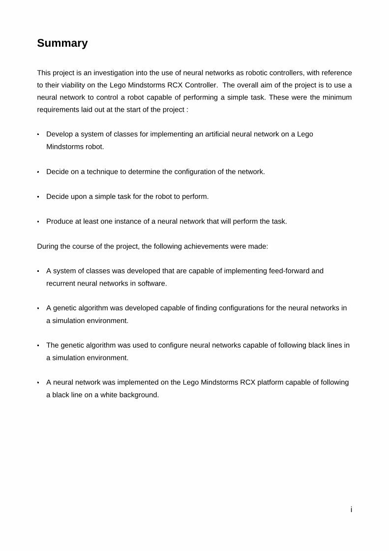
Summary

This project is an investigation into the use of neural networks as robotic controllers, with reference

to their viability on the Lego Mindstorms RCX Controller. The overall aim of the project is to use a

neural network to control a robot capable of performing a simple task. These were the minimum

requirements laid out at the start of the project :

� Develop a system of classes for implementing an artificial neural network on a Lego

Mindstorms robot.

� Decide on a technique to determine the configuration of the network.

� Decide upon a simple task for the robot to perform.

� Produce at least one instance of a neural network that will perform the task.

During the course of the project, the following achievements were made:

� A system of classes was developed that are capable of implementing feed-forward and

recurrent neural networks in software.

� A genetic algorithm was developed capable of finding configurations for the neural networks in

a simulation environment.

� The genetic algorithm was used to configure neural networks capable of following black lines in

a simulation environment.

� A neural network was implemented on the Lego Mindstorms RCX platform capable of following

a black line on a white background.

i

Acknowledgments

I would like to thank my project leader Tony Cohn for his guidance and support. Thanks to Tom

Carden for providing me with an excellent simulation environment. To Seth Bullock and Jason

Noble whose stimulating lectures sparked my interest in bio-inspired computing, and to the rest of

the Bio-systems Reading Group - Dave Harris, John Cartlidge, Dan Franks, and Neil Meckle for

their inspiring discussions and patience when I didn't know what they were talking about.

ii

Table of Contents

Summary....................................................................................................................................i

Acknowledgments....................................................................................................................ii

Table of Contents....................................................................................................................iii

Chapter 1 - Introduction...........................................................................................................1

1.1 The Problem..................................................................................................................1

1.2 Lego Mindstorms and the RCX Controller..................................................................1

1.3 Neural Networks............................................................................................................2

1.4 The Advantages of Using Neural Networks for Autonomous Robots......................6

1.5 Configuration Methods..................................................................................................7

1.6 Previous Work Using Neural Networks for Robot Control........................................8

1.7 The Layout of This Report............................................................................................8

Chapter 2 – Design..................................................................................................................9

2.1 The Design of the Task................................................................................................9

2.2 The Choice of Configuration Method........................................................................10

2.3 The Robot....................................................................................................................10

Chapter 3 - The Neural Network..........................................................................................12

3.1 Design..........................................................................................................................12

3.2 Implementation............................................................................................................13

Chapter 4 - The Simulation...................................................................................................16

4.1 Design..........................................................................................................................16

4.2 Assumptions................................................................................................................17

4.3 Implementing the Simulation......................................................................................17

Chapter 5 - The Genetic Algorithm......................................................................................22

5.1 The Fitness Function .................................................................................................23

5.2 The Selection Routine................................................................................................24

iii

5.3 The Method of Generating a New Population..........................................................25

5.2 Implementation of the Genetic Algorithm.................................................................26

Chapter 6 - Results................................................................................................................29

6.1 A Network Created by Thinking About What Might Work. .....................................29

6.2 Not So Successful GA Networks...............................................................................31

6.3 The Most Successful GA Net.....................................................................................32

Chapter 7 - Transferring the network to the Lego Mindstorms Robot..............................35

Chapter 8 - Conclusion..........................................................................................................37

8.1 Neural Networks..........................................................................................................37

8.2 Genetic Algorithms......................................................................................................37

8.3 Simulations..................................................................................................................37

Chapter 9 - Evaluation...........................................................................................................38

9.1 Was this project successful?......................................................................................38

9.2 Future Work.................................................................................................................38

9.3 Practical uses of this project......................................................................................39

References..............................................................................................................................40

Appendix A..............................................................................................................................43

Appendix B The Code Used to Implement the Neurons....................................................44

Appendix C The Code Used to Implement the Genetic Algorithm....................................49

iv

Chapter 1 - Introduction

1.1 The Problem

The design of robot controllers has turned out to be much more problematic than modern

science fiction ever envisaged. Machines have been developed which excel at processing a

single stream of data, with computer power measured in instructions per second doubling

approximately every 18 months. This is a fantastic acheivement, but this type of processor

does not fare well when presented with the complexities of a physical environment. The

problems of the real world can be thought of as orthogonal to the problems of a super

calculator. The calculator solves one group of very similar problems over and over again.

The real world poses many different problems, perhaps all at the same time, and maybe for

the first and last time. Similarly, the calculator processes one small data group at a time, for

example it might have to work with two numbers using arithmetical logic. The robot

controller is presented with a multitude of data items, such as the pixels in a video stream.

This data must be combined somehow into a description of the state of the world and used

to generate a reaction or course of action. The programming required for artificial

intelligence tasks is therefore very different to the programming for number-crunching

programs (Brooks, 1991). This is one reason why the field of robotics has made slow

progress in comparison to other computer-related fields. Artificial neural networks are a

different way of programming robots, because instead of explicitly stating the conditions

which indicate a given situation has arisen and the exact motor responses required, the

programmer creates a network of small decision-making modules which each have a small

influence over how the robot will act. The robot's actions result from a combination of the

outputs of these modules. Researchers and private individuals have reported some success

in using neural networks to control robots. This project is an attempt to replicate some of

those successes using the Lego Mindstorms RCX controller.

1.2 Lego Mindstorms and the RCX Controller

Lego Mindstorms is a product designed for building and programming robots. The RCX

controller is a large Lego brick containing the computer that controls the robot. The RCX

1

was inspired by the programmable brick developed at MIT Media Lab, which receives

funding from Lego (Martin). It is marketed primarily as a toy but also provides a cost-

effective platform for robotics research.

The neural networks were written in software using an implementation of the C

programming language written specifically for use with the RCX. The RCX comes with a

programming tool which uses graphical representations of standard programming

structures, which look a bit like lego blocks. The user builds his program as a combination of

these blocks. This tool is very simple to use, because it has been built to help children get

used to programming. It does not offer the flexibility required to implement neural networks

because there is no provision for declaring and using variables, so NQC was used as the

programming language. NQC stands for Not Quite C. It is fairly well established now with

support for Linux, Windows and Macintosh computers, and was developed by David

Baum.

1.3 Neural Networks

Artificial neural networks are an attempt to model the working of a brain. Throughout this

project, it is to be assumed of any references to networks or neural networks that the

intended meaning is artificial neural networks. Neural networks consist of one or more

nodes which function in a similar way to neurons in the brain. They also have one or more

input units and one or more output units. A node accepts a number of inputs, either from the

input units or from other nodes, which are individually weighted. Simple nodes can be in one

of two states, passive or active. Initially the output is 0, which represents the passive state.

When the sum of the weighted inputs reaches a threshold, the node is triggered and the

output changes to 1. This represents the active state, or firing, of the node. The simplest

neural network has one node, and is referred to as the single layer perceptron. The single

layer perceptron was proposed in 1943 by McCulloch and Pitts.

2

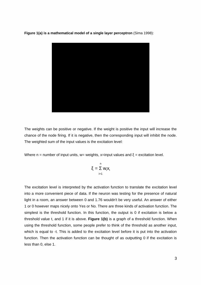
Figure 1(a) is a mathematical model of a single layer perceptron (Sima 1998):

The weights can be positive or negative. If the weight is positive the input will increase the

chance of the node firing. If it is negative, then the corresponding input will inhibit the node.

The weighted sum of the input values is the excitation level:

Where n = number of input units, w= weights, x=input values and ξ = excitation level.

n

ξ = Σ wixii=1

The excitation level is interpreted by the activation function to translate the excitation level

into a more convenient piece of data. If the neuron was testing for the presence of natural

light in a room, an answer between 0 and 1.76 wouldn't be very useful. An answer of either

1 or 0 however maps nicely onto Yes or No. There are three kinds of activation function. The

simplest is the threshold function. In this function, the output is 0 if excitation is below a

threshold value t, and 1 if it is above. Figure 1(b) is a graph of a threshold function. When

using the threshold function, some people prefer to think of the threshold as another input,

which is equal to -t. This is added to the excitation level before it is put into the activation

function. Then the activation function can be thought of as outputting 0 if the excitation is

less than 0, else 1.

3

The threshold function is suitable for single layer networks or where the output is a 'yes or

no' type of answer. There are two other kinds of activation function, linear and sigmoid. In

linear functions (Figure 1(c) ) the output is proportional to the weighted input. In sigmoid

functions (Figure 1(d) ), the output varies but not in proportion to the input (Hinton, 1992).

The benefit of using these functions is that more information about the original excitation

level is passed forward to the next layer of nodes. This is neccessary when using

techniques such as the back-propagation technique (discussed in section 1.5) for training

neural networks (Beale and Jackson).

Figures 1(b), 1(c), and 1(d) ( 1(d) taken from Matthews, J, labels added). These are the

actvation functions that are commonly used when modelling neurons.

4

Figure 1(e) is a simple neural network implementing an AND function (Sima 1998):

Figure 1(e) is a simple neural network implementing a boolean AND function. The inputs

are all weighted at 1 so their contributions will either be one or zero. If all of the inputs to the

network are 1 the total weighted inputs will be n. After addition of the threshold (-n) this will

be 0. When this is evaluated using the threshold function, the output will be 1, because n - n�

0. If any of the inputs are 0, � will be less than 0, and the output will be 0. The network

only produces an input of 1 if all of the inputs are 1, which is the correct implementation of

an AND function.

We can think of the neuron as a simple decision making module. If the inputs satisfy the

requirements for the neuron to fire, the output is 1. Otherwise, the output is 0. In order to

make more complex decisions it is necessary to use more nodes. Nodes are grouped in one

or more layers. The layout of the nodes is referred to as the topology of the network. The

values and distribution of the weights is referred to as the configuration of the network (Sima

1998).

Some general types of neural network have been defined that aid discussion of the topic in

general. Feed Forward networks are those in which all the nodes in one layer are connected

to all the nodes in the next, with data flowing in one direction from the input layer to the

output layer. This design is the easiest type of network to consider the working of. Recurrent

neural networks have nodes with outputs connected to themselves and to nodes in layers

which are upstream in the general flow of data. This gives the network a sort of memory, an

awareness of the world's state prior to the present situation. There are also GasNets, which

5

have nodes capable of modelling the use of gas in the brain. They use this to communicate

to all the nodes within the distribution limits of the gas. The gas also has a time factor in that

the nearest nodes will be affected immediately, whereas those at the limits of the gases

reach will be affected much later. GasNets are a recent development of neural networks,

and much less work has been done using them than the other types.

1.4 The Advantages of Using Neural Networks for Autonomous Robots.

Neural networks can be fairly confusing particularly if the topology is complex. It seems

perhaps illogical to take something that is difficult to do, like programming a robot, and make

it more complicated by introducing a method that is poorly understood. However there are

advantages to using neural networks.

Autonomous robots have limited practical application at the moment, it seems unlikely that

they will be trusted to operate in situations where they interact with humans or are

responsible for the safety of people. One area where they have been used is exploration,

sending a robot where it is too dangerous or too expensive to send a human. In these

situations it is vitally important that the robot is robust. The standard computer architecture is

not particularly robust, because the loss of one unit can lead to total failure for the entire

machine. Neural networks have been shown to degrade gracefully (Beer) which means that

if parts of the network are compromised the other bits can continue to function with

performance degrading gradually as losses are incurred. It is conceivable that such a robot

in a hazardous territory could lose a component and continue to operate, completing the

mission in a longer time or perhaps even repairing itself.

Autonomous Robots in such an exploratory role would probably have to cope with sensor

data that was unreliable and subject to levels of random noise. This is a problem for robot

programmers because it is difficult to describe a situation accurately in order to specify the

motor outputs required to deal with it if the inputs are likely to be varied. Neural networks

have been shown to cope well with noisy data, even using it to their advantage (Cliff). This is

partly because the nodes in a network make decisions based on a function of more than one

input, so if one is abnormally high it has little effect on the overall working of the network.

The division of processing power between the nodes in a multiprocessor system means that

much lower processing power can be used. One of the problems people writing robot

controllers using centralized computer architectures have found is that processing power is

quickly used up in modeling the situation to decide what to do next, causing what Brooks

termed the “representational bottleneck”. Neural networks avoid this eventuality by

6

dispensing with representing the world situation internally and by dividing the processing

between the nodes. Suitable controllers developed using neural networks would therefore

not have the same requirement for the most advanced computer components available,

meaning they could be developed at a much lower cost.

1.5 Configuration Methods

Determing the configuration of the network is a complicated task. The complexity increases

exponentially as the number of nodes increases, because each node is connected to every

other node. As Harvey et al state, humans are not designed for or used to thinking about

complex systems such as these. To overcome this difficulty, various researchers have

developed systems for the configuration of neural networks. The simplest is trial and error,

adjusting the weights of each node until the network functions more or less correctly. This

approach has been used successfully for simple networks, but if the network is large then

this approach becomes tedious and haphazard (James 1995, Hoffman).

Around 1974 Paul Werbos invented the back-propagation algorithm. A sample set of data is

presented to the network for which the desired output is already known. The actual output of

the network is then compared to the desired results, and the weights are adjusted from the

output nodes back through the network, in order to reduce the error (Hinton 1992).

The genetic algorithm (GA) is a system used to configure networks with little or no tweaking

of the weights directly by the network's developer. A network's configuration is specified by a

genotype, typically a string of digits representing the weights at each node. A random

population of networks is generated and tested either in simulation or as an embodied

agent. A fitness function is the test used to determine which genotypes will be used to

create the next generation. For example, if you were trying to evolve an exploration robot,

the fitness function might be based on how far the robots move. The genotypes from the top

scorers are then reproduced using cloning, mixing and minor random mutations to make the

next generation, which is usually the same size as the first. Using this Darwinian system the

population gradually improves until an optimal system is reached. Genetic algorithms have

been used successfully to evolve neural networks for controlling robots (Floreano,

Husbands, Beer).

7

1.6 Previous Work Using Neural Networks for Robot Control

Here are a few examples of people who have reported success using neural networks for

robot control. Beer produced a "dynamical systems perspective" for describing the

interaction between a robot and its environment. He demonstrated that the networks could

maintain states which changed over time and with interactions with the environment,

allowing it to react to a sequence of events rather than just the current state. Beer et al

produced a network for controlling a hexapod robot that used information from sensors on

the limbs to vary the gait of the robot. The robot demonstrated that neural networks are

robust because it was capable of dealing with the loss of some sensory data. Under these

conditions the neural network's performance degraded gracefully - the gait worsened with

the loss of components but still functioned.

Husbands et al made GasNets that could discriminate between simple shapes drawn on a

screen. The networks would propel a robot towards a triangle, but ignore a rectangle. The

networks were compared to other networks which did not use gas modelling, and were

much less complicated than their standard counterparts when producing similar behaviour.

They could be evolved much more quickly because of this reduction in complexity.

Webb made a robot cricket which demonstrated the tracking response to a mating call using

a much simpler neural pattern than most biologists had previously thought was required. It

would move towards only one source of cricket song even if more were present, as

observed in real crickets, and could differentiate between songs of different frequencies.

This demonstrated the cross-disciplinary worth of studying neural networks, and together

with the GasNets shows how advances in neuroscience and using biologically inspired

computer controllers can benefit both disciplines.

1.7 The Layout of This Report

The following report is modular in structure, reflecting the work supporting it. It was initially

written with a large design chapter and a large implementation chapter. This meant that

references in the two chapters were awkward to go back and forth between. It was decided

that it made more sense for the reader if all of the material concerning an individual part of

the project, for example the genetic algorithm, was in one section. Furthermore the report's

structure now allows the reader to dip into the report and read just the parts they are

interested in. If he or she only wants to know about the genetic algorithm, then all the

material on that topic is nicely grouped together.

8

Chapter 2 – Design

The first decision that needed to be made was what task was going to be set for therobot to perform.

2.1 The Design of the Task

Here are the criteria that were considered important for the task that was to be attempted:

� The first task should be possible using the equipment available.� The first task should be fairly simple so that if the controller does not work it is

possible to understand why. � The first task should be complicated enough so that it could not happen by

chance, so that we can say the network is controlling the robot.� It should be simple to evaluate the controller's performance at the task so that it is

easy to say that one robot is better at the task than another.

There are a number of tasks that are often attempted by people who are developing robot

controllers. It was decided that one of these would be suitable, because they are proven to

be achievable using the sort of equipment available. Here is a list of some of the most

popular:

� Move towards or away from a light source.� Find a particular object, or avoid bumping into an object.� Follow a line which has been drawn on the floor.

It was decided that 'following a black line on a white background' fulfills all of the criteria

required to be the task. It is not possible that the robot could perform this without the

intervention of a suitable controller, because the direction of the robot has to be changed

over time according to the direction the line travels in. The task is fairly simple however, and

can probably be performed using a fairly basic neural network. The fact that the task can be

performed over a given length of time as opposed to a task that has a finite length will make

the evaluation of early stages easier. For example, a robot that searches for an object could

be doing some proper searching but in the wrong direction. If the robot was being evaluated

according to its proximity to the object after a given time it might score lower than a robot

9

that didn't move but happened to start in the right place.

2.2 The Choice of Configuration Method

Trial and error was not considered to be a suitable configuration method because it is not a

systematic way to proceed and does not seem like a sound method or one that would scale

up to more complicated networks. The back-propagation technique is more appropriate for

designing neural networks for classifier systems because of its reliance upon a known set of

inputs and corresponding outputs. In the case of a robot controller this sample set of data is

difficult to generate because there are rarely absolutely correct answers in real life

situations. As there has already been a tremendous amount of work done using back-

propagation the decision was taken not to study this technique here. For this project a

genetic algorithm was used to configure the neural networks, because it seemed the most

interesting method and the most appropriate way to achieve the stated objectives.

Running a genetic algorithm involves producing a population of genotypes and then testing

each one to determine the fitness that the corresponding phenotype would have. The genes

are then selected for reproduction, and a new population seeded. Although the process can

be described fairly quickly, the process of testing each individual can be very time

consuming, especially if a large population is used. The process can take many runs and is

very repetitive. For this reason the process was carried out in simulation.

2.3 The Robot

The RCX has three input ports and three output ports. The input ports can be connected to

sensors that give the robot information about its environment, such as light or touch

sensors. Information from these sensors will provide the input for the neural network. Motors

can be attached to the three output ports. These motors are connected to actuators for

example limbs or wheels which the robot uses to interact with its environment. The output

from the neural network will be used to control the actuators.

The physical design of the robot is important because it affects the robot's ability to interact

with the environment. It is also non-trivial because some of the designs I have seen have

been quite complicated. However, a full investigation of potential designs is beyond the

bounds of this project, so the design is only referred to here to provide a specification for the

10

robot and an explanation of how it works.

There are two large wheels powered by two motors either side of the middle of the robot.

The robot can steer by adjusting the power to either wheel. This was considered to be the

easiest way to implement steering. A steering rack similar to the one found on a car could

have been used, with one of the motors controlling forward motion and one controlling

direction. The design chosen was less complicated to engineer and provided a more direct

correlation between light sensor reading and motor output. It was therefore deemed to be

more suitable for a neural network to control.

At one end there is a pair of light sensors that point at the floor. One of the main problems

with this sort of equipment is the inconsistency of the ambient light present. For example, on

a dark day, the light readings will be very different to on a bright sunny day. For this reason,

the light sensors have a small light source attached to them. This is very useful for line

detection, because it means that the light reading is more dependent upon the floor's light-

reflecting properties than the rooms ambient light levels as long as the light sensor is close

enough to the surface. The first design that I built did not have the sensors close enough to

the floor, so I rebuilt the arms holding the light sensors so that they were approximately half

a centimetre clear of the floor. This meant that the contrast detected between the black line

and the background was greatly improved.

11

Chapter 3 - The Neural Network

3.1 Design

The intention was to use the simplest design possible particularly at first, to encourage

understanding of what is happening within the network. However there are minimal sizes of

neural network that are capable of controlling a robot. The single layer perceptron, although

a useful classifier based on multiple inputs, only produces one output and is therefore not

capable of controlling two motors independently. The network will need at least two output

nodes, one to control each motor. It would be possible for a robot to display line following

behaviour using just one light sensor and employing a sweeping motion to detect line

direction. However this is a fairly complex behaviour pattern and would require a recurrent

network so that the robot could compare the current result to a previous one. It was decided

that the simplest network capable of line following will be one that accepts two light sensors

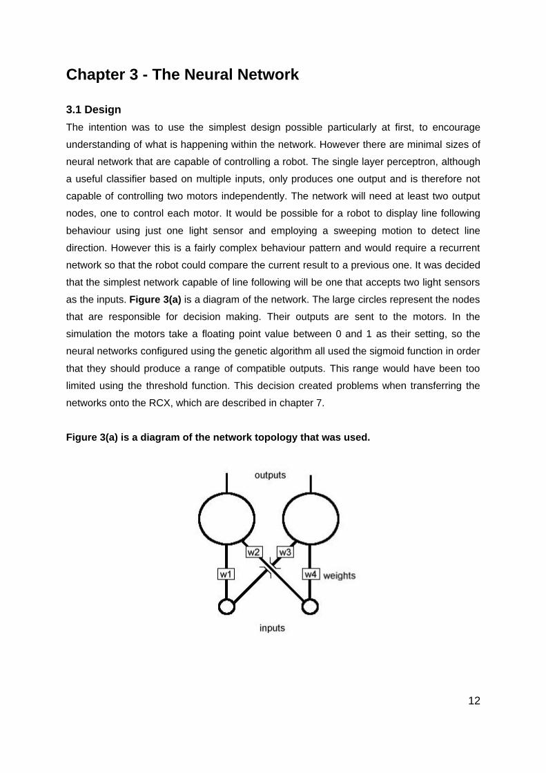
as the inputs. Figure 3(a) is a diagram of the network. The large circles represent the nodes

that are responsible for decision making. Their outputs are sent to the motors. In the

simulation the motors take a floating point value between 0 and 1 as their setting, so the

neural networks configured using the genetic algorithm all used the sigmoid function in order

that they should produce a range of compatible outputs. This range would have been too

limited using the threshold function. This decision created problems when transferring the

networks onto the RCX, which are described in chapter 7.

Figure 3(a) is a diagram of the network topology that was used.

12

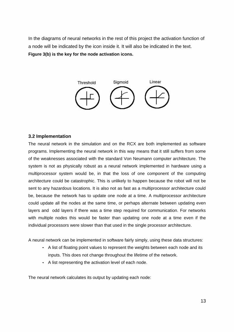
In the diagrams of neural networks in the rest of this project the activation function of

a node will be indicated by the icon inside it. It will also be indicated in the text.

Figure 3(b) is the key for the node activation icons.

3.2 Implementation

The neural network in the simulation and on the RCX are both implemented as software

programs. Implementing the neural network in this way means that it still suffers from some

of the weaknesses associated with the standard Von Neumann computer architecture. The

system is not as physically robust as a neural network implemented in hardware using a

multiprocessor system would be, in that the loss of one component of the computing

architecture could be catastrophic. This is unlikely to happen because the robot will not be

sent to any hazardous locations. It is also not as fast as a multiprocessor architecture could

be, because the network has to update one node at a time. A multiprocessor architecture

could update all the nodes at the same time, or perhaps alternate between updating even

layers and odd layers if there was a time step required for communication. For networks

with multiple nodes this would be faster than updating one node at a time even if the

individual processors were slower than that used in the single processor architecture.

A neural network can be implemented in software fairly simply, using these data structures:� A list of floating point values to represent the weights between each node and its

inputs. This does not change throughout the lifetime of the network. � A list representing the activation level of each node.

The neural network calculates its output by updating each node:

13

� Calculating the product of each input and its corresponding weight� Summing all of the products� Evaluating this value using the activation function

This process begins with the input layer, and works its way sequentially through the nodes

to the output layer. This ensures that the input layer for each node has been updated before

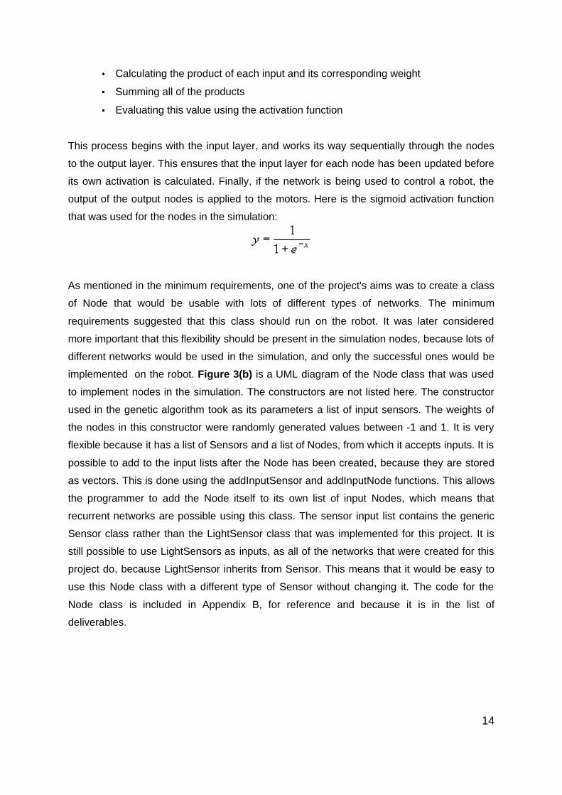
its own activation is calculated. Finally, if the network is being used to control a robot, the

output of the output nodes is applied to the motors. Here is the sigmoid activation function

that was used for the nodes in the simulation:

As mentioned in the minimum requirements, one of the project's aims was to create a class

of Node that would be usable with lots of different types of networks. The minimum

requirements suggested that this class should run on the robot. It was later considered

more important that this flexibility should be present in the simulation nodes, because lots of

different networks would be used in the simulation, and only the successful ones would be

implemented on the robot. Figure 3(b) is a UML diagram of the Node class that was used

to implement nodes in the simulation. The constructors are not listed here. The constructor

used in the genetic algorithm took as its parameters a list of input sensors. The weights of

the nodes in this constructor were randomly generated values between -1 and 1. It is very

flexible because it has a list of Sensors and a list of Nodes, from which it accepts inputs. It is

possible to add to the input lists after the Node has been created, because they are stored

as vectors. This is done using the addInputSensor and addInputNode functions. This allows

the programmer to add the Node itself to its own list of input Nodes, which means that

recurrent networks are possible using this class. The sensor input list contains the generic

Sensor class rather than the LightSensor class that was implemented for this project. It is

still possible to use LightSensors as inputs, as all of the networks that were created for this

project do, because LightSensor inherits from Sensor. This means that it would be easy to

use this Node class with a different type of Sensor without changing it. The code for the

Node class is included in Appendix B, for reference and because it is in the list of

deliverables.

14

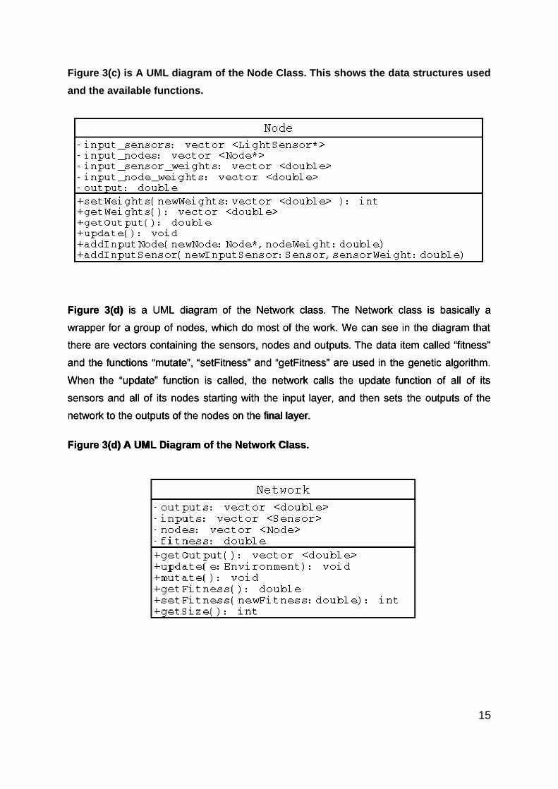
Figure 3(c) is A UML diagram of the Node Class. This shows the data structures used

and the available functions.

Figure 3(d) is a UML diagram of the Network class. The Network class is basically a

wrapper for a group of nodes, which do most of the work. We can see in the diagram that

there are vectors containing the sensors, nodes and outputs. The data item called “fitness”

and the functions “mutate”, “setFitness” and “getFitness” are used in the genetic algorithm.

When the “update” function is called, the network calls the update function of all of its

sensors and all of its nodes starting with the input layer, and then sets the outputs of the

network to the outputs of the nodes on the final layer.

Figure 3(d) A UML Diagram of the Network Class.

15

Chapter 4 - The Simulation

4.1 Design

Jakobi puts forward a set of criteria for designing minimal simulations. The guiding principle

is that elements of the simulation which are necessary for the agent to demonstrate the

required behaviour should be present and as little else as possible. The reasons for using

this method in this project are listed here:

� The controller needs to be able to make decisions based on limited information,

so it is not necessary to simulate lots of information.� If the simulation is complex, the controller could be taking advantage of a flaw in

the simulation rather than using the environmental characteristics of the

simulation to perform the task.� A complex simulation which attempts to simulate the real world comprehensively

will take longer to create and longer to run. As the goal of simulation is to save

time compared to actually carrying out the experiment, this reduces its validity

(Jakobi).� It is the simplest way to progress.

It was decided that the elements of the robot's interaction with the environment that needed

to be simulated in order to develop a robot capable of demonstrating line following

behaviour were the following:

� The robot should be in an environment which contains a black line for it to follow.� The motor outputs should be based upon the inputs received from the light

sensors. The light sensor readings will need to reflect the robot's situation in

relation to the black line. If the robot is over a black line, the result returned by the

light sensor should be lower than if it is over white space.� In order for the robot to demonstrate line following behaviour, the motor outputs

should be interpreted as propelling the robot, and the robot's position should be

adjusted accordingly.

Jakobi goes on to explain that in order to ensure that the controller can reliably transferred

from the simulation to the real world it is necessary to randomly change the parameters

16

governing interaction between the robot and its environment in the simulation. For example,

if there was a value for adjusting the level of friction between the wheels and the floor, then

this could be randomly adjusted after each generation, simulating a range of surfaces. This

is to make sure that the controller has been tested with as many different parameters as

possible. The aim is to ensure that the controller has demonstrated that it works when the

parameters are as close as possible to the real life parameters. This part of the procedure

was not followed because of the time limit involved in the project and the simplicity of the

task and the simulation. This is also referred to in the Future Work part of the Evaluation

chapter.

4.2 Assumptions

Here is a list of the assumptions that were made when designing and implementing the

simulation.

1. In the simulation there is a direct correlation between the output the controller

gives for the motor and the movement of the robot. In reality the robot's progress

would be affected by friction or a lack of it between the floor and the tyres,

fluctuations in battery output and other hardware flaws.

2. The readings from the light sensors are not affected by the ambient light in the

room. In reality there is a base level of light present which generates a minimum

reading for the light sensors. In the simulation if the light sensor is reading from a

part of the image composed entirely of black pixels the reading is zero.

3. The light sensors in the simulation return data which is one hundred percent

reliable. In reality the data would be affected by random noise due to the

limitations of the sensors, which are not heavily insulated or tested to a high

degree of accuracy.

4.3 Implementing the Simulation

The basis for the simulation was a project written by another student, Tom Carden. He has

written a simulation environment with robots that can move around and sense each other,

intended for developing flocking algorithms and to be extended for other purposes. This

provided the modeling of the movement for the simulation used in this project because the

17

robots featured moved in the same way as my robot, with two motors driving two wheels

and a caster wheel for support. It also provided a framework for proceeding in an object

oriented way with developing the parts that were specific to my requirements. Object

oriented programming allows more code re-use. Carden's code contains a class called a

Sensor, which he has extended to make a Robot Sensor. The Robot Sensor has the same

data types and functions as the Sensor without reproducing the original code. The sensor

that was implemented for this project was a Light Sensor, so the Sensor class was extended

to give it the abilities specific to a Light Sensor. Deitel and Deitel's C++ How To Program

has a more detailed explanation of object oriented programming.

Calculating the Movement of the robots

The robot's steering is controlled using a differential drive system. This means that there are

two wheels on either side of the robot which are independently controlled by two motors,

providing motion and directional control (Lucas).

Carden's code for determining the movement of the robot was used without modification,

with the exception that in the first step the motor controls were updated from the neural

network. At each time step, the program goes through this routine to see how far the robot

has moved:

Where L = left wheel speed

R = right wheel speed

A = acceleration

V = velocity

RC = rotation constant = 2*PI

AC = acceleration constant = 5000

RV = rotation velocity (how fast the robot's direction is changing)

T = time step (how much time passes between loops)

1. Update the motor controls with the output of the controller

2. Calculate rotation velocity RV = L - R * RC

3. Calculate acceleration A = (L + R)/2 * AC

4. Adjust the robot's velocity V = A * T

5. Adjust the robot's orientation orientation += RV * T

6. Adjust location by velocity location += V * T

18

The system is an efficient way to estimate the movement of a differential-drive system. In

step 2 the rotation is calculated as the difference between the left motor output and the right

motor output (see Figure 4(a) ). In step 3 the acceleration is calculated as the average of

the two motor outputs. Step 4 changes the velocity of the robot by the acceleration

calculated in step 3, and steps 5 and 6 calculate the new orientation of the robot and then

move it by an amount proportional to the velocity. Although at step 6 it treats the trajectory

as a straight line, the distance is small and the error will therefore be fairly low. Treating the

trajectory as a curve would involve more calculation for little gain in accuracy (Lucas). The

exact values used for the rotation and acceleration constants are not that important, as long

as they are appropriate. Carden's choices worked well, and were not changed.

Figure 4(a) is a diagram showing that the rotation produced is dependent on the

difference between the two motor outputs. (G. W. Lucas, some minor modifications).

Adding the Line to the Simulation

Updating the simulation environment to put a line on the floor involved extending the

Scenery class to make a class called FloorPlan. This takes an image file and draws it on the

background of the simulation. This is done before all of the other drawing so that it does not

cover up the other elements of the scene. The image is composed of pixels which are either

white (representing the background) or black (representing the line).

The FloorPlan class generates two arrays of integers, one containing the X values of every

black pixel, and one containing all of the Y values. The arrays are generated by examining

the RGB value of each pixel in the image in turn, and adding it's coordinates to the arrays if

the red value is equal to 0. It is only necessary to use the red pixel values because the

19

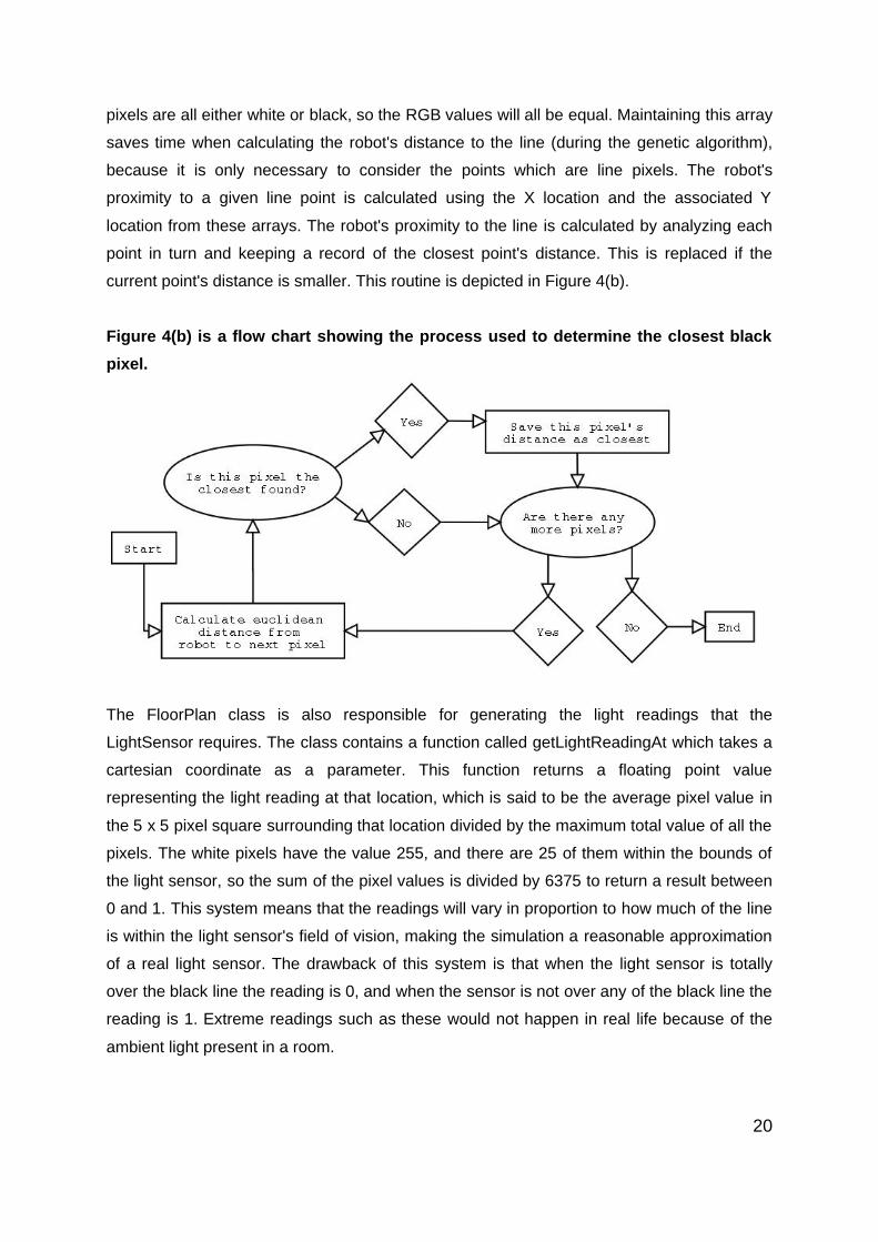
pixels are all either white or black, so the RGB values will all be equal. Maintaining this array

saves time when calculating the robot's distance to the line (during the genetic algorithm),

because it is only necessary to consider the points which are line pixels. The robot's

proximity to a given line point is calculated using the X location and the associated Y

location from these arrays. The robot's proximity to the line is calculated by analyzing each

point in turn and keeping a record of the closest point's distance. This is replaced if the

current point's distance is smaller. This routine is depicted in Figure 4(b).

Figure 4(b) is a flow chart showing the process used to determine the closest black

pixel.

The FloorPlan class is also responsible for generating the light readings that the

LightSensor requires. The class contains a function called getLightReadingAt which takes a

cartesian coordinate as a parameter. This function returns a floating point value

representing the light reading at that location, which is said to be the average pixel value in

the 5 x 5 pixel square surrounding that location divided by the maximum total value of all the

pixels. The white pixels have the value 255, and there are 25 of them within the bounds of

the light sensor, so the sum of the pixel values is divided by 6375 to return a result between

0 and 1. This system means that the readings will vary in proportion to how much of the line

is within the light sensor's field of vision, making the simulation a reasonable approximation

of a real light sensor. The drawback of this system is that when the light sensor is totally

over the black line the reading is 0, and when the sensor is not over any of the black line the

reading is 1. Extreme readings such as these would not happen in real life because of the

ambient light present in a room.

20

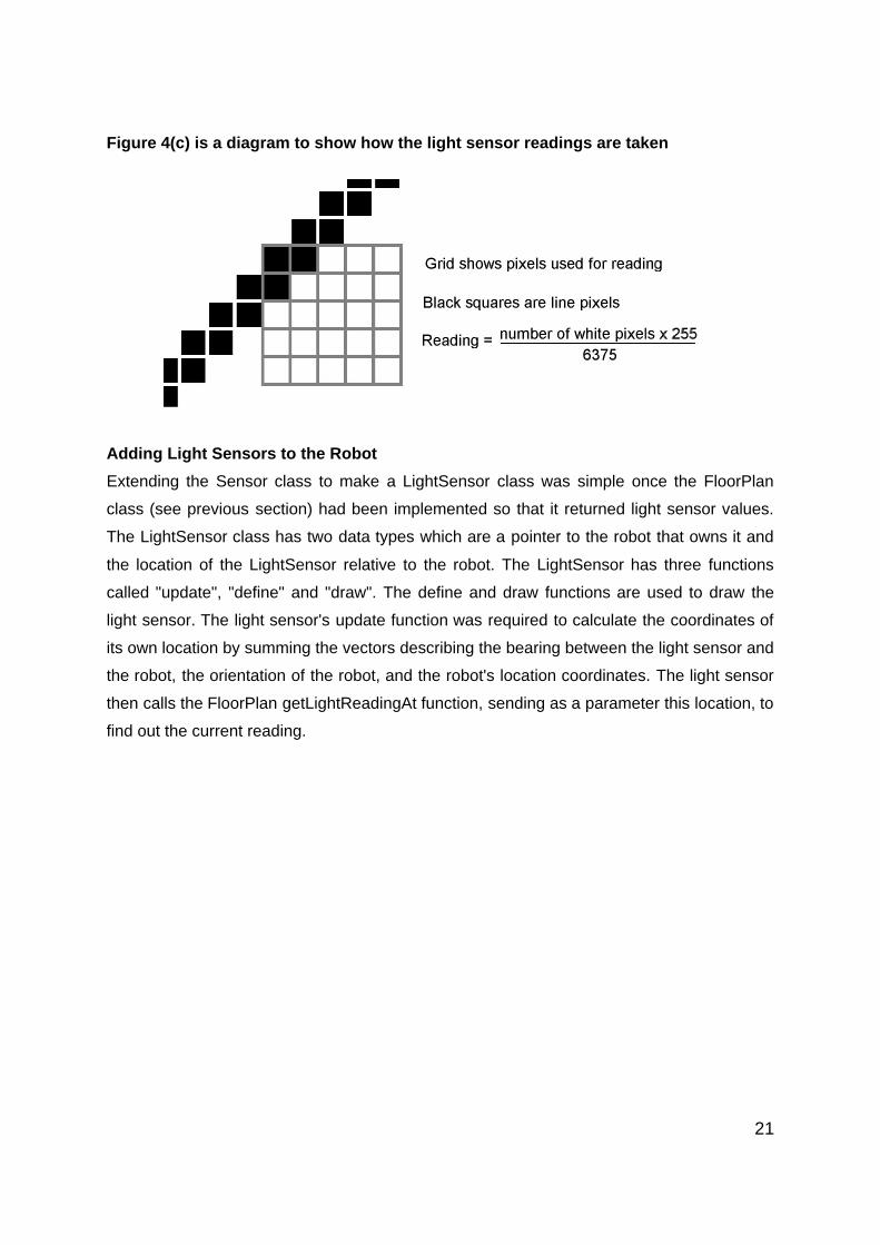
Figure 4(c) is a diagram to show how the light sensor readings are taken

Adding Light Sensors to the Robot

Extending the Sensor class to make a LightSensor class was simple once the FloorPlan

class (see previous section) had been implemented so that it returned light sensor values.

The LightSensor class has two data types which are a pointer to the robot that owns it and

the location of the LightSensor relative to the robot. The LightSensor has three functions

called "update", "define" and "draw". The define and draw functions are used to draw the

light sensor. The light sensor's update function was required to calculate the coordinates of

its own location by summing the vectors describing the bearing between the light sensor and

the robot, the orientation of the robot, and the robot's location coordinates. The light sensor

then calls the FloorPlan getLightReadingAt function, sending as a parameter this location, to

find out the current reading.

21

Chapter 5 - The Genetic Algorithm

A genetic algorithm is an evolutionary system. Noble highlights Darwin's requirements for an

evolutionary system to work:

1. Heredity

2. Variation

3. Selection

Heredity means that individuals have similar characteristics to their parents. To make sure

that the individuals in a genetic algorithm have this characteristic, an encoding scheme of

their properties is used which describes their characteristics, rather like DNA. It can be

copied in whole or in part to give descendants similar traits. It must be capable of expressing

the entire search space and be easily generated and manipulated. An individuals

characteristics expressed in the encoding scheme is referred to as the genotype. The

physical counterpart of the genotype (the individual itself) is referred to as the phenotype.

The networks were limited to one particular topology so it was only necessary to express the

weights of the network. The genotype for each network consisted of four floating point

values, each corresponding to one of the weights in the network.

Variation means that individuals are different. This is present in the genetic algorithm

because the encoding scheme is capable of expressing more than one type of individual,

and the members of the population are created with random properties. Variation is

maintained from generation to generation by random mutations.

Selection means that some individuals are more likely to reproduce than others. Selection in

a genetic algorithm is achieved using a combination of the fitness function and the selection

procedure.

The fitness function, the selection routine and the reproduction cycle will be treated here

individually to avoid confusion. They are each as important as each other, because the

algorithm does not work if any one is missing or poorly implemented. This can cause

problems when you are writing the GA, because if it doesn't work it is difficult to know which

part of the genetic algorithm is at fault. Furthermore, due to the repetitive nature of the

genetic algorithm, small problems in one of these parts can be amplified during the iterations

to create a larger problem.

22

5.1 The Fitness Function

The purpose of the fitness function is to apply selective pressure to a population. Selective

pressure occurs when certain members of a population have characteristics that make them

more likely to succeed in reproducing than others. Selective pressure is used in a genetic

algorithm to influence reproduction so that individuals emerge with the required

characteristics or abilities. The fitness function in the genetic algorithm used in this project

allocates each member of the population a score depending on their performance during a

period of testing. These scores are then used in the selection routing to ensure that the fitter

individuals have more chance of reproducing.

Writing a fitness function which rewards the behaviour you are looking for is fairly difficult

even when the behaviour and the network are simple. This is the first fitness function that

was used:

� Calculate the distance to the nearest line pixel. � Calculate the distance traveled since the last interval. � Divide the distance traveled by the distance to the nearest pixel to get the score

for this time step. � Fitness is equal to the average score.

The fitness function was designed to reward robots that remained on or near the line. It was

also considered important to make sure that the robot would not move onto the black line

and then remain there until the time ran out. When this fitness function was used however,

the robots that evolved traveled very quickly along paths that curved by varied amounts.

They totally ignored the line, although sometimes the motor output would read a slight blip

as they went over it. This behaviour is logical considering the way the fitness function and

their environment worked. There was only a certain distance that the robots could go from

the line because of the wall surrounding the environment. It seemed that by gaining points

for travelling very fast they could compensate for any points lost by not actually being on the

line. The circular trajectory was probably encouraged by the fact that if they hit a wall and

stopped they would lose points for not moving. The ones that were turning would move

round and run off in the other direction. This fitness function was tried with different

thicknesses and shapes of line with no success.

The next fitness function was similar, but this time the robot was only rewarded for moving if

it was on the line, or at least within five pixels. This gave rise to much the same behaviour

23

as the previous function, although it was noted that the robot's path was normally a similar

sized circle to the one that the line drew. This was moderately encouraging, because it at

least indicated that the GA was capable of producing different robots, and that it might be

close to working properly.

It was noted that the robots were traveling too fast for the line to have much of an effect on

their motion, so the reward for moving was removed. In the next fitness function the only

way the robots would score points after each time step would be by being near to the line.

To reduce the chances of robots being rewarded for having the fortune to start on the line

the robots would be tested at 10 different locations in the picture. This also meant that good

robots would not be penalized for starting in a bad place. The time period that each robot

was tested for during each test was reduced, because the good robots would either find the

line in the first minute or not at all, due to the simplicity of the search method. The final

fitness function looked like this:

� Start the robot at a random location � Calculate the distance to the line� Score for this time step is the inverse of this distance� Repeat the above 10 times� Fitness is the average score

This fitness function is incredibly simple, because it just amounts to giving the robots points

for being near the line. This works in this situation because the network is so simple. There

was no need to reward the robots for moving because it was very unlikely that a robot would

evolve that could move onto the line and stop. A node using the sigmoid function used in

this project only outputs a number close to 0 if the excitation level is below -5. As the light

readings vary between 0 and 1 this would only happen with weights so low they were never

obtained by any of the networks developed in the genetic algorithm.

Keeping the fitness function as simple as possible has a similar benefit to keeping the

simulation minimal. It means that it is harder for the controllers to take advantage of a flaw in

the fitness function in order to increase their fitness without performing the task. With a more

complicated task however it is unlikely that one this simple would work.

5.2 The Selection Routine

The selection routine determines which genotypes will be included (wholly or in part) in the

24

next population. There are many types of selection routine to consider, but they normally

have a lot in common with these main types:

� Elitism – the highest scoring genotypes are selected.� Tournament selection – groups of genotypes from the population are chosen

randomly, and the one with the highest score is selected.� Roulette wheel selection – each genotype's chance of reproduction is equal to his

own fitness as a percentage of the groups fitness.

When choosing a selection routine it is important to consider the size of the population, the

amount of variation possible within the genetic encoding method, and the method of

reproduction. It was decided that a large population would not be required, because the

level of diversity possible within the genetic encoding scheme was fairly small. Initially the

selection routine used was elitism, because this seemed like the routine that would apply the

most evolutionary pressure on the population. The problem that was observed when using a

small population and elitism for selection was that after very few generations there was very

little variation within the population. The evolutionary pressure was too great to allow genetic

variation within the gene pool. It is important that the evolutionary pressure should allow

some networks that do not score as highly to reproduce, because two good solutions will not

always have similar genetic encodings. In order for other good solutions to be found it is

necessary to allow the genetic algorithm to search through poor solutions. Tournament

selection was implemented and it was observed that the genetic algorithm was

searching a reasonable section of the gene pool after the reproduction method had

been selected (see below).

5.3 The Method of Generating a New Population

In order to satisfy the an evolutionary system's requirement for heredity, it is necessary to

use some reproduction when generating the new population. As the random genotypes

created when the genetic algorithm is started are unlikely to include the entire genetic

search space, genotypes are normally mutated at random to increased the chances of other

parts of the search space being tested. A low percentage chance of mutation is normally

used, and mutations are normally by a low amount, so that their influence does not cancel

out the work of reproduction. At first it was decided that each genotype would have a 10%

chance of having one of its floating point values mutated by a random value between -0.1

25

and 0.1.

Reproduction can be sexual or asexual. Sexual recombination means that genotypes are

generated as a combination of two or more genotypes from the previous generation. This

was the method that was used when the first genetic algorithm was implemented. It was

soon noted that the weights of the neural networks it was producing had little or no variation

after very few generations. This is because the population and the amount of variation

possible was very small. Each sexual recombination reduces the variation present in the

population, because at each reproduction one genotype is produced from two genotypes.

Asexual reproduction means that each selected individual's genotype is copied into the new

population without being combined with another's. This method was used to try to reduce

the amount of convergence. In order to ensure that the GA would search through a larger

part of the search space, the rate of mutation was increased so that every genotype would

have one of its floating point values mutated before being put back into the gene pool.

5.2 Implementation of the Genetic Algorithm

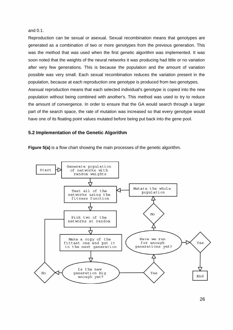
Figure 5(a) is a flow chart showing the main processes of the genetic algorithm.

26

A population of individuals was generated randomly, and each one was ran in the simulation

environment for an equal amount of time. At each time step the robot's situation was

assessed using the fitness function. Then the selection routine was used to select the

fortunate individuals who would be contributing to the new generation. Then the new

population was created, and the process repeated until the specified number of generations

had been completed. The size of the population and the number of generations was

adjusted quite a few times during the first few runs, but settled at about 20 individuals and

about 30 generations. Often the genetic algorithm was halted early if it seemed like there

was little variation present in the population or between two generations. The final code for

the genetic algorithm is included in Appendix B, for reference and because it was in the list

of deliverable items for the project.

When I started writing the genetic algorithm, a class called Genotype was implemented to

use as an encoding system for the weights of the nodes. The realization was made that this

class held nearly exactly the same data as the Network class did, and that the copying of

this data from the Network class to the Genotype for the purposes of reproduction and then

back to the Network class for testing was a complete waste of processor time. The functions

and data in the Genotype class that were necessary for the genetic algorithm to function

were moved into the Network class.

The picture that was used, which is analogous to the environment that the robot was

developing in, was very important. If a picture with a line that was too thin was used, the

robots didn't react to it. If the line was too thick, the fitness function would take a lot longer to

run. The final adjustment that was made before actually getting the genetic algorithm to

work was increasing the number of lines in the picture, so that it was more likely that the

robot would run over the line and it would have a chance to follow it. Care was taken to

ensure that there was space at the edge of the picture for robots that weren't very good at

line following to flounder in so there was no possibility of them getting jammed into a corner

with part of the line in it and scoring highly despite their inability.

It would seem from this report that the implementing the genetic algorithm was a fairly

straightforward procedure, but this is not the case. Many combinations of fitness function,

selection procedure, reproduction method and line image were tried before one that worked

quite well was found, and all the time bug checking had to be performed to check that a

code error was not stopping the algorithm from working. A genetic algorithm can be very

time consuming if you have little experience of them, and because the solution always

27

seems to be just around the corner it is easy to spend much more time doing it than is

justified for finding the solution to a simple problem like the one discussed here. Hopefully,

the difficulty involved in writing one becomes less and less the more familiar you are with

them. I found the advice offered to me by people who had already done them to be very

useful, which supports this theory.

28

Chapter 6 - Results

As mentioned previously, many of the networks that were created just went round in circles

of varying sizes. This is in part due to the simplicity of the networks. There is no recurrency

in the network which would allow it to be aware of previous states, so the network can only

react to the two current readings. More complex behaviour would require more connections

between the nodes, or more nodes. There are only really three situations the network can

be in:

� The left light sensor's reading is higher � The right light sensor's reading is higher� The readings are the same

The resulting behaviour can only be a combination of the reactions to these situations, with

the reactions being more or less pronounced depending on the degree of inequality between

the two readings.

6.1 A Network Created by Thinking About What Might Work.

Whilst work was being done to get the genetic algorithm to work, a set of weights was

thought of and tried them out in the simulation. The weights worked quite well. Here are the

weights of Network A:

Figure 6(a) is a diagram of Network A.

29

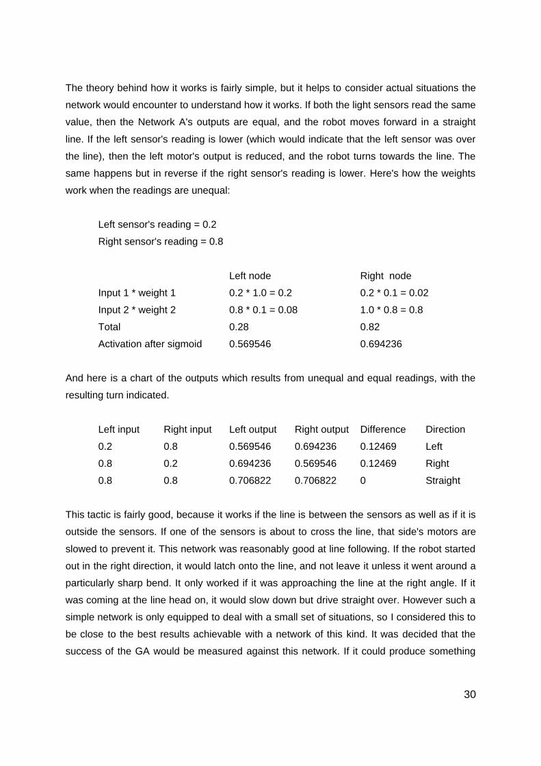
The theory behind how it works is fairly simple, but it helps to consider actual situations the

network would encounter to understand how it works. If both the light sensors read the same

value, then the Network A's outputs are equal, and the robot moves forward in a straight

line. If the left sensor's reading is lower (which would indicate that the left sensor was over

the line), then the left motor's output is reduced, and the robot turns towards the line. The

same happens but in reverse if the right sensor's reading is lower. Here's how the weights

work when the readings are unequal:

Left sensor's reading = 0.2

Right sensor's reading = 0.8

Left node Right node

Input 1 * weight 1 0.2 * 1.0 = 0.2 0.2 * 0.1 = 0.02

Input 2 * weight 2 0.8 * 0.1 = 0.08 1.0 * 0.8 = 0.8

Total 0.28 0.82

Activation after sigmoid 0.569546 0.694236

And here is a chart of the outputs which results from unequal and equal readings, with the

resulting turn indicated.

Left input Right input Left output Right output Difference Direction

0.2 0.8 0.569546 0.694236 0.12469 Left

0.8 0.2 0.694236 0.569546 0.12469 Right

0.8 0.8 0.706822 0.706822 0 Straight

This tactic is fairly good, because it works if the line is between the sensors as well as if it is

outside the sensors. If one of the sensors is about to cross the line, that side's motors are

slowed to prevent it. This network was reasonably good at line following. If the robot started

out in the right direction, it would latch onto the line, and not leave it unless it went around a

particularly sharp bend. It only worked if it was approaching the line at the right angle. If it

was coming at the line head on, it would slow down but drive straight over. However such a

simple network is only equipped to deal with a small set of situations, so I considered this to

be close to the best results achievable with a network of this kind. It was decided that the

success of the GA would be measured against this network. If it could produce something

30

that was as good at line following as the network above, I would be able to say that it had

worked.

6.2 Not So Successful GA Networks

There were many unsuccessful networks that the GA developed before it was fine-tuned to

its peak performance. Even then it would produce networks of varying performance.

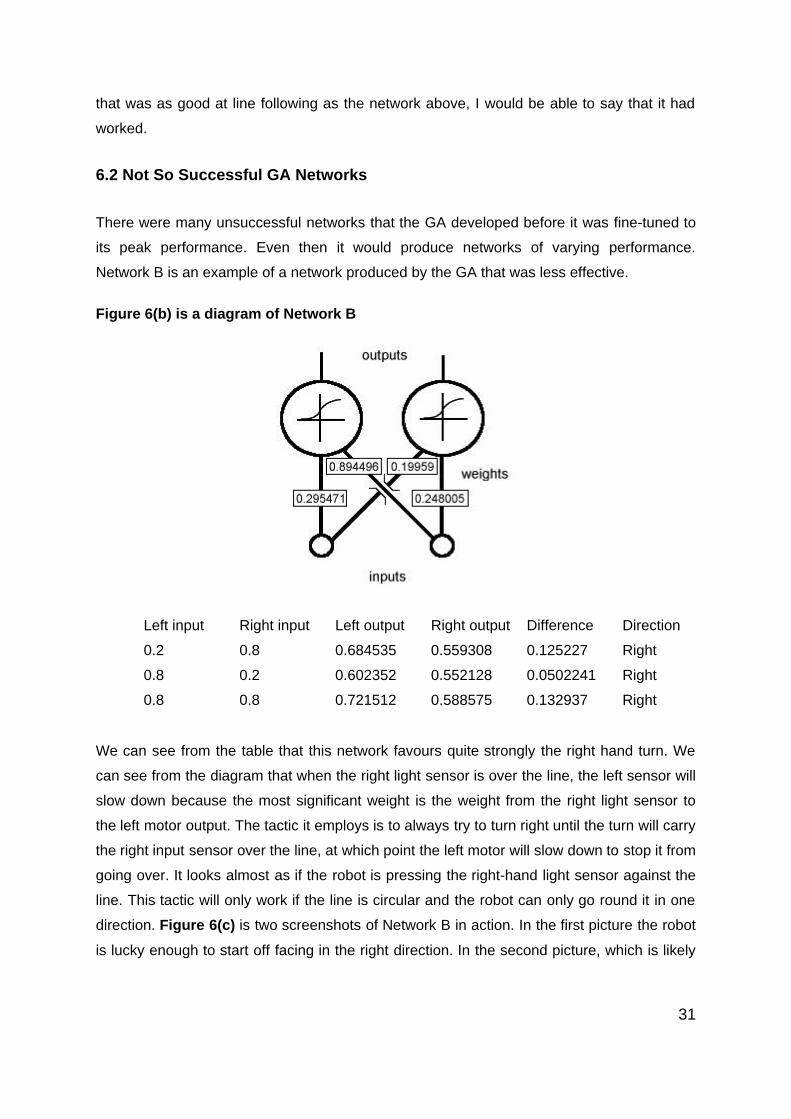
Network B is an example of a network produced by the GA that was less effective.

Figure 6(b) is a diagram of Network B

Left input Right input Left output Right output Difference Direction

0.2 0.8 0.684535 0.559308 0.125227 Right

0.8 0.2 0.602352 0.552128 0.0502241 Right

0.8 0.8 0.721512 0.588575 0.132937 Right

We can see from the table that this network favours quite strongly the right hand turn. We

can see from the diagram that when the right light sensor is over the line, the left sensor will

slow down because the most significant weight is the weight from the right light sensor to

the left motor output. The tactic it employs is to always try to turn right until the turn will carry

the right input sensor over the line, at which point the left motor will slow down to stop it from

going over. It looks almost as if the robot is pressing the right-hand light sensor against the

line. This tactic will only work if the line is circular and the robot can only go round it in one

direction. Figure 6(c) is two screenshots of Network B in action. In the first picture the robot

is lucky enough to start off facing in the right direction. In the second picture, which is likely

31

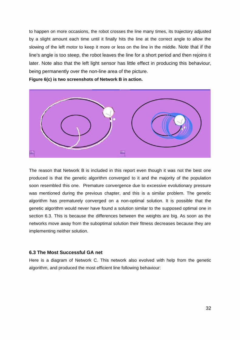
to happen on more occasions, the robot crosses the line many times, its trajectory adjusted

by a slight amount each time until it finally hits the line at the correct angle to allow the

slowing of the left motor to keep it more or less on the line in the middle. Note that if the

line's angle is too steep, the robot leaves the line for a short period and then rejoins it

later. Note also that the left light sensor has little effect in producing this behaviour,

being permanently over the non-line area of the picture.

Figure 6(c) is two screenshots of Network B in action.

The reason that Network B is included in this report even though it was not the best one

produced is that the genetic algorithm converged to it and the majority of the population

soon resembled this one. Premature convergence due to excessive evolutionary pressure

was mentioned during the previous chapter, and this is a similar problem. The genetic

algorithm has prematurely converged on a non-optimal solution. It is possible that the

genetic algorithm would never have found a solution similar to the supposed optimal one in

section 6.3. This is because the differences between the weights are big. As soon as the

networks move away from the suboptimal solution their fitness decreases because they are

implementing neither solution.

6.3 The Most Successful GA net

Here is a diagram of Network C. This network also evolved with help from the genetic

algorithm, and produced the most efficient line following behaviour:

32

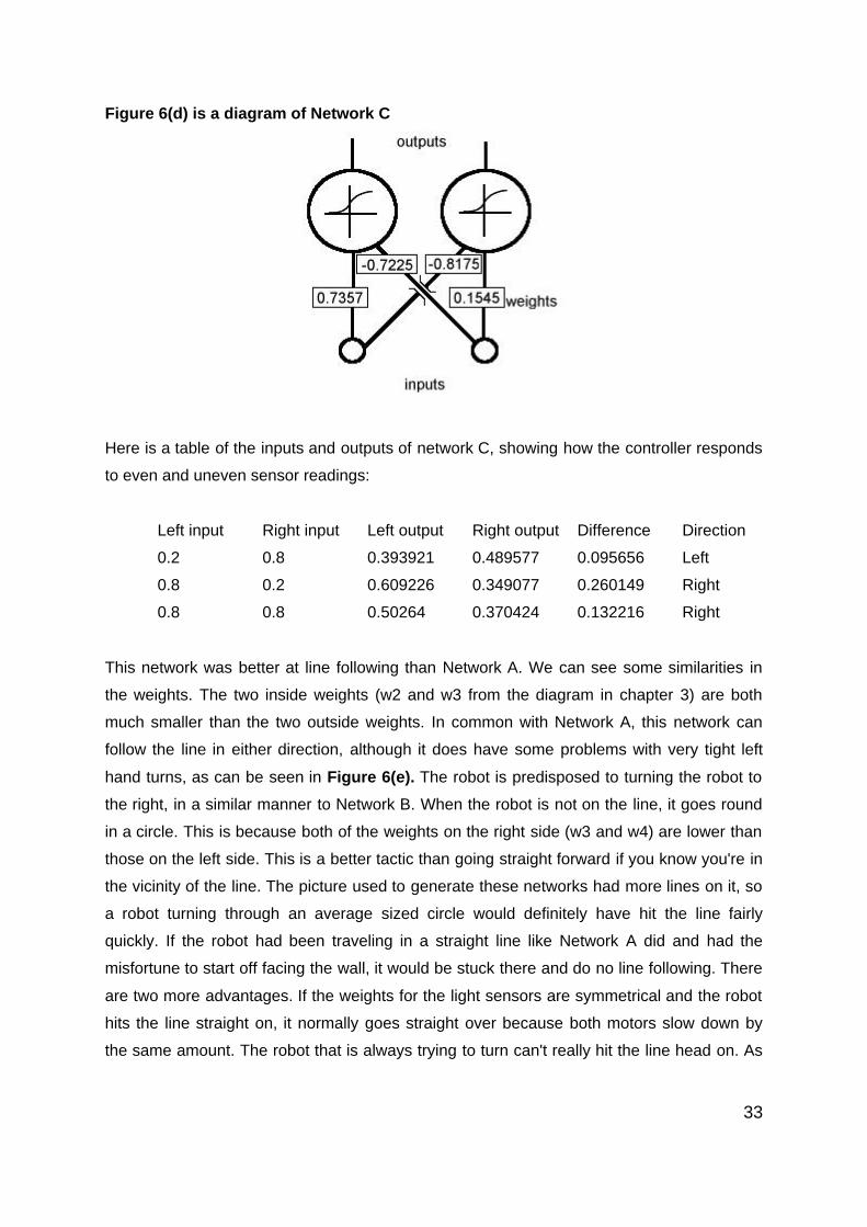
Figure 6(d) is a diagram of Network C

Here is a table of the inputs and outputs of network C, showing how the controller responds

to even and uneven sensor readings:

Left input Right input Left output Right output Difference Direction

0.2 0.8 0.393921 0.489577 0.095656 Left

0.8 0.2 0.609226 0.349077 0.260149 Right

0.8 0.8 0.50264 0.370424 0.132216 Right

This network was better at line following than Network A. We can see some similarities in

the weights. The two inside weights (w2 and w3 from the diagram in chapter 3) are both

much smaller than the two outside weights. In common with Network A, this network can

follow the line in either direction, although it does have some problems with very tight left

hand turns, as can be seen in Figure 6(e). The robot is predisposed to turning the robot to

the right, in a similar manner to Network B. When the robot is not on the line, it goes round

in a circle. This is because both of the weights on the right side (w3 and w4) are lower than

those on the left side. This is a better tactic than going straight forward if you know you're in

the vicinity of the line. The picture used to generate these networks had more lines on it, so

a robot turning through an average sized circle would definitely have hit the line fairly

quickly. If the robot had been traveling in a straight line like Network A did and had the

misfortune to start off facing the wall, it would be stuck there and do no line following. There

are two more advantages. If the weights for the light sensors are symmetrical and the robot

hits the line straight on, it normally goes straight over because both motors slow down by

the same amount. The robot that is always trying to turn can't really hit the line head on. As

33

well as that, if a robot using this controller goes over the line or leaves the line at a sharp

bend it goes round in a circle and has another chance to rejoin it. This can take several

passes with the robot's path being adjusted by a small amount each time it circles, due to

contact with the line. This robot was better at line following than Network A, so the genetic

algorithm was judged to be successful in finding a line following solution. Network C took a

lot longer to develop than Network A, but was a better solution overall.

Figure 6(e) is two screenshots of Network C in action. The same light sensor is being used

to follow the line in both cases, despite the fact that the robot is traveling in different

directions. In the picture on the right, the robot has left the line and later rejoined it.

34

Chapter 7 - Transferring the network to the LegoMindstorms RobotOnce Network A was working, the possibilities of getting it to work on the Lego Mindstorms

platform were investigated. It was soon discovered that there would have to be a few

changes in the way the network on the robot worked. The Lego Mindstorms outputs work in

integers only, using a function called SetPower. It is possible to set the power of the motors

to an integer from 0 to 7 inclusive. In fact, in NQC there is no provision for using floating

point values at all. This presents two difficulties. Firstly, the sigmoid function used for the

activation levels of the network delivers a floating point value between 0 and 1, which can't

be calculated as an integer. Secondly, the motors in the simulation could be set to a floating

point value between 0 and 1, giving a good deal more possibilities than eight different

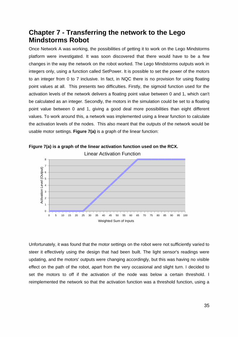
values. To work around this, a network was implemented using a linear function to calculate

the activation levels of the nodes. This also meant that the outputs of the network would be

usable motor settings. Figure 7(a) is a graph of the linear function:

Figure 7(a) is a graph of the linear activation function used on the RCX.

Unfortunately, it was found that the motor settings on the robot were not sufficiently varied to

steer it effectively using the design that had been built. The light sensor's readings were

updating, and the motors' outputs were changing accordingly, but this was having no visible

effect on the path of the robot, apart from the very occasional and slight turn. I decided to

set the motors to off if the activation of the node was below a certain threshold. I

reimplemented the network so that the activation function was a threshold function, using a

35

0 5 10 15 20 25 30 35 40 45 50 55 60 65 70 75 80 85 90 95 100

0

1

2

3

4

5

6

7

8

Linear Activation Function

Weighted Sum of Inputs

Act

ivat

ion

Leve

l (O

utpu

t)

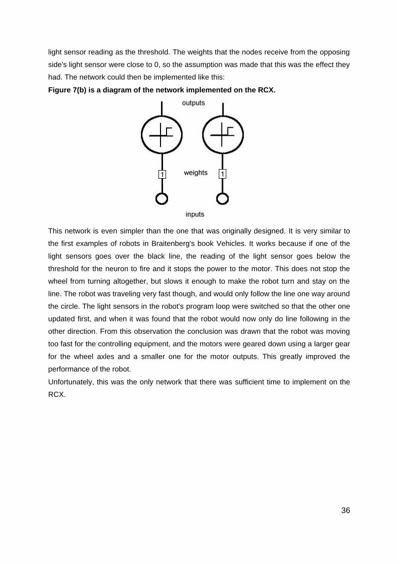
light sensor reading as the threshold. The weights that the nodes receive from the opposing

side's light sensor were close to 0, so the assumption was made that this was the effect they

had. The network could then be implemented like this:

Figure 7(b) is a diagram of the network implemented on the RCX.

This network is even simpler than the one that was originally designed. It is very similar to

the first examples of robots in Braitenberg's book Vehicles. It works because if one of the

light sensors goes over the black line, the reading of the light sensor goes below the

threshold for the neuron to fire and it stops the power to the motor. This does not stop the

wheel from turning altogether, but slows it enough to make the robot turn and stay on the

line. The robot was traveling very fast though, and would only follow the line one way around

the circle. The light sensors in the robot's program loop were switched so that the other one

updated first, and when it was found that the robot would now only do line following in the

other direction. From this observation the conclusion was drawn that the robot was moving

too fast for the controlling equipment, and the motors were geared down using a larger gear

for the wheel axles and a smaller one for the motor outputs. This greatly improved the

performance of the robot.

Unfortunately, this was the only network that there was sufficient time to implement on the

RCX.

36

Chapter 8 - Conclusions

8.1 Neural Networks

Neural networks can be used to design robot controllers and have the potential to create

robust and flexible solutions. However they are not easy to design or configure and

therefore it is necessary to use special techniques when developing them.

8.2 Genetic Algorithms

Genetic algorithms can be used to solve problems that humans find difficult to think about.

Genetic algorithms are one technique that can be used to configure neural networks. Using

a genetic algorithm in conjunction with neural networks it is not neccessary to program the

robot with the ability to detect when situations have arisen and specify all of the

corresponding motor outputs. Unfortunately, the genetic algorithm is not without its own

problems:

� The genetic algorithm can take a long time to run(Boers). � The fitness function is not easy to write. It may be more interesting to specify the

behaviour you would like to see at a higher level than motor outputs, but if you

spend more time writing the fitness function than it would have taken you to

program the robot's behaviour in the standard way it is hard to justify the use of a

such a convoluted technique(Zaera et al). � There is no guarantee of success(Zaera et al).

8.3 Simulations

A simulation environment can be used to automate the procedure, removing the necessity

for someone to perform a mundane and repetitive testing procedure. However it is important

that the robot architecture is examined before the simulation is created to ensure that it is

modelled accurately.

37

Chapter 9 - Evaluation

9.1 Was This Project Successful?

Here are the minimum requirements that were specified at the beginning of the project:

1. Build a suitable robot incorporating the Lego Mindstorms RCX Brick.

2. Develop a class library which implements a neuron. This should :

i. Be connectable to any number of other neurons.

ii. Process inputs to produce outputs.

iii. Be able to accept multiple inputs and outputs.

3. Design a simple task for the robot to perform.

4. Investigate the techniques which have been developed to configure artificial

neural networks.

5. Using one or a combination of the techniques from part 4 as a starting point,

develop a network using the class library from part 2 which can perform the task

in part 3.

6. Evaluate the design of the robot and the approach taken.

If these minimum requirements are used as the criteria to judge the success of the project it

is fair to say that it has been successful, as all of the minimum requirements have been met.

9.2 Future Work

Future directions that could be taken to extend this project include the following:

Some time could be spent making the simulation more realistic. As mentioned in the

assumptions, real sensors do not return accurately predictable results. Jakobi proposes that

simulation parameters be adjusted at random to ensure that a network capable of dealing

with the various situations is created. This aspect could be incorporated by adding random

noise to the light readings. After each generation, the probability of it occuring would be

adjusted.

Recurrent neural networks could be used to control the robot. A recurrent neural network

would allow the network to exhibit more complex behaviour. Using a recurrent network, it

38

might be possible to get the robot to use a better strategy for searching for the line. It might

be able to use a side to side sweeping pattern for example, and then change to a more

reactive strategy when the line was found. Implementing recurrent networks in the

simulation would not be too difficult, because of the flexibility that was built into the software

produced in this project.

GasNets could be developed , although this would require some extension to the classes

used to implement the networks.

It would be interesting to implement a controller using electronic components for the

neurons instead of using the RCX. It would be possible to test the robustness of the setup

by removing components to see how this affected its performance.

9.3 Practical Uses of This Project

Neural networks of the sort used during this project are too simple to have applications

controlling a robot in which they the only control structure of the robot. It is unlikely that

someone would be trying to program a line following robot without success. This project is

modular in structure, and I think that this is how a neural network as simple as the one

developed in this project could find a purpose in the real world. A network as simple as the

ones discussed here could be used to control part of a robot that was built as separate

modules. For example, it could control a camera on top of an exploring robot, to make sure

it was always pointing towards a light part of the scene, so that as much information was

received as possible.

Another possibility of a modular use for this sort of network could be in a subsumption

architecture as proposed by Brooks. There would be many small neural networks connected

to the same inputs and outputs. The networks are ranked according to their importance, and

can only affect the robot's actions if there are no higher ranking networks trying to influence

the robot. In this way, many small types of behaviours could be combined into a more

complex set.

Finally, Bonabeau et al suggest artificial systems could be implemented using group

interactions to generate apparently intelligent systems from collections of organisms

exhibiting simple behaviours. It is conceivable that swarm systems could be created capable

of complex tasks, using artificial agents controlled by networks as simple as the ones used

in this project and configured using similar techniques.

39

References

Baum, D, Not Quite C Homepage, http://www.enteract.com/~dbaum/nqc/index.html

[March 2002]

Beer, R D, Chiel, H J, Quinn, R D, Espenschied, K and Larsson, P, (1992) A Distributed

Neural Net Architecture For Hexapod Robot Locomotion, Neural Computation, M.I.T.

Press, Vol. 4, pp. 356-365

Beer, R, (1995), A Dynamical Systems Perspective on Agent-Environment Interaction, in:

Artificial Intelligence, 72:173-215 (sections 1,2 & 3).

Beer,R and Gallagher, J, (1992), Evolving Dynamical Neural Networks for Adaptive

Behaviour, Adaptive Behavior, 1(1):91--122

Bonabeau, E, Dorigo, M and Théraulaz, G (1999). Swarm Intelligence: From Natural

to Artificial Systems. Oxford University Press.

Braitenberg, V, (1986), Vehicles: Experiments in Synthetic Psychology. MIT Press

Brooks, R,(1991), Intelligence without Reason, in: The Artificial Route to Artificial

Intelligence, Steels, L, Brooks, R, Lawrence Erlbaum Associates

Brooks, R, (1991b), Intelligence without representation, Artificial Intelligence, 47(1--

3):139--159

Bullock, S, AR35 Bio-Inspired Computing Lecture Notes,

http://www.comp.leeds.ac.uk/seth/ar35/ [March 2002]

Deitel, H, and Deitel, Paul, (1998), C++ How To Program Second Edition, Prentice Hall

Floreano, D and Mondada, F, Evolution of Homing Navigation in a Real Robot, in: IEEE

Transactions on Systems, Man and Cybernetics, Vol 26, Number 3, June 1996, pp 396-

407

40

Husbands, P, Smith, T, Jakobi, N, O'Shea, M, (1998), Better Living Through

Chemistry:Evolving GasNets for Robot Control in: Ziemke, T. and Sharkey, N.E. (editors),

Connection Science Special Issue: BioRobotics 10(3-4): 185-210, Carfax

Husbands, P, Cliff, D, Thompson, A and Jakobi, N, Evolutionary Robotics: the Sussex

Approach, in: Robotics and Autonomous Systems, v. 20 (1997) pp. 205

Hinton, G, (1992) How Neural Networks Learn from Experience, in: Scientific American

September 1992 pp105-109.

Hoffman, F, (1997) Evolutionary Learning of Mobile Robot Behaviours, First Workshop on

Frontiers in Evolutionary Algorithms FEA97,

http://www.nada.kth.se/~hoffmann/fea97.ps.gz

James, J, Dagli, C, (1995) Use of Genetic Algorithms for Encoding Effective Neural

Networks Architectures: Neuro-Computer Implementation, in: SPIE Proceedings of

Applications and Science of Artificial Neural Networks, p. 323-330, Orlando, Florida.

Lucas, GW, http://rossum.sourceforge.net/papers/DiffSteer/DiffSteer.html[April 2002]

Martin, F, Unofficial Questions and Answers about MIT Programmable Bricks and LEGO

Mindstorms, http://web.media.mit.edu/~fredm/mindstorms/, [April 2002]

Matthews, J, Generation5 website Neural Networks Essays,

http://www.generation5.org/essays.shtml#nn[April 2002]

Noble, J, AR35 Bioinspired Computing Lecture 11 Evolutionary Design 1,

http://www.comp.leeds.ac.uk/seth/ar35/syllabus/topic6.html[April 2002]

Sima, J, (1998) Introduction to Neural Networks. Technical report V-755, ICS CAS, Prague.

Smith, T, Philippides, A, (2000), Nitric Oxide Signalling in Real and Artificial Neural

Networks, British Telecom Technology Journal, 18 (4):140-149

41

Webb, B, (1996), A robot cricket, in:Scientific American, 275(6), 94-99

Zaera, N, Cliff, D, and Bruten, J, (1996) (Not) Evolving Collective Behaviors in Synthetic

Fish, in: Maes, P, Mataric, M, Meyer, J-A, Pollack, J, and Wilson, S, (editors) From Animals

to Animats 4: Proceedings of the Fourth International Conference on Simulation of

Adaptive Behavior (SAB96), MIT Press Bradford Books, pp.635--644

42

Appendix A

My personal motivation for doing this project was to have a greater understanding of how

neural networks and genetic algorithms worked, and whether it would be possible for me to

reproduce some of the inspiring work I had read about during the AR35 course. I have

definitely achieved the first part of this, but I did expect to do more of the second part than I

ended up doing. I would have liked to have spent more time actually working with the robot.

If I hadn't had to spend so much time implementing the genetic algorithm I might have been

able to move onto a more complex task with the robot. I think I underestimated the amount

of time it would take me to implement the basic techniques that are described in this report.

This project has been a great experience for me and was an opportunity to put into practice

the object oriented techniques that we learnt in the programming modules. Here is a list of

the main lessons I will take away from it:

Test classes before they are included in the rest of your program. This can be done easily

using a simple function that just calls the constructor, performs the functions in the code,

outputs the results and then exits. This can save a good deal of bug fixing time in the long

run.

Getting involved with other people in your line of work helps you to progress. Open

discussion with people working in fields relating to this project was extremely helpful for me,

because it inspired me with ideas that I might not otherwise have thought of.

Make sure you provide yourself with feedback if you are implementing a long-running

program like a genetic algorithm by outputting to the screen at appropriate intervals. You will

be able to see if there is a problem, and maybe have a guess at what it is.

If you are using more than one type of architecture, don't make assumptions about their

capabilities or compatibilities. If I had investigated the programming of the RCX more

thoroughly, my simulation would have transferred to the robot a lot more easily.

When attempting a large coding project, one day of planning will be more productive and

less frustrating than a week of reimplementation due to poor design.

43

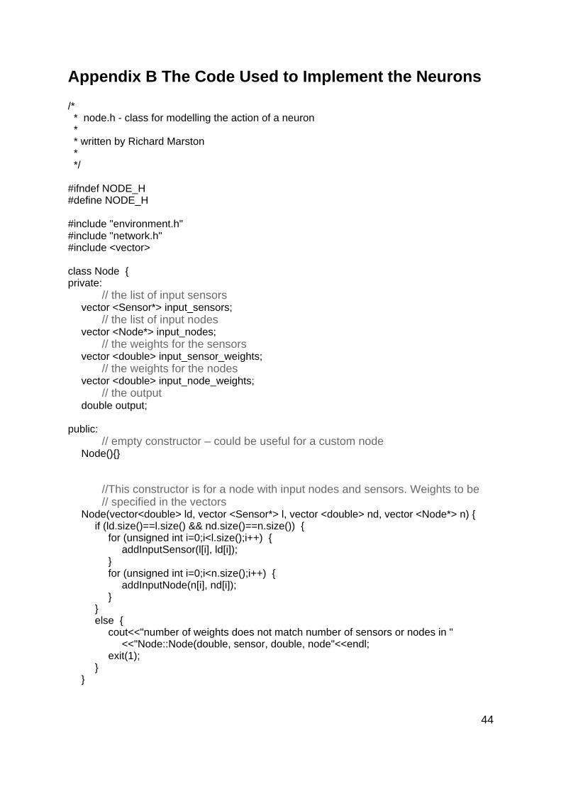
Appendix B The Code Used to Implement the Neurons

/* * node.h - class for modelling the action of a neuron * * written by Richard Marston * */

#ifndef NODE_H#define NODE_H

#include "environment.h"#include "network.h"#include <vector>

class Node {private:

// the list of input sensorsvector <Sensor*> input_sensors;

// the list of input nodesvector <Node*> input_nodes;

// the weights for the sensorsvector <double> input_sensor_weights;

// the weights for the nodesvector <double> input_node_weights;

// the outputdouble output;

public:// empty constructor – could be useful for a custom node

Node(){}

//This constructor is for a node with input nodes and sensors. Weights to be // specified in the vectors

Node(vector<double> ld, vector <Sensor*> l, vector <double> nd, vector <Node*> n) {if (ld.size()==l.size() && nd.size()==n.size()) {

for (unsigned int i=0;i<l.size();i++) {addInputSensor(l[i], ld[i]);

}for (unsigned int i=0;i<n.size();i++) {

addInputNode(n[i], nd[i]);}

}else {

cout<<"number of weights does not match number of sensors or nodes in "<<"Node::Node(double, sensor, double, node"<<endl;

exit(1);}

}

44

// This constructor is for a node with sensors only. Weights must be specifiedtoo.

Node(vector <double> d, vector <Sensor*> l) {if (d.size()==l.size()) {

for (unsigned int i=0;i<l.size();i++) {addInputSensor(l[i], d[i]);

}}else {

cout<<"number of weights does not match number of sensors in "<<"Node::Node(vector<double>, vector<sensor*>"<<endl;

exit(1);}

}

//This constructor is for a node with sensors. Random weights are allocatedNode(vector <Sensor*> l) {

for (unsigned int i=0;i<l.size();i++) {addInputSensor(l[i], (double)rand()/RAND_MAX);

}}

//This constructor is for a node with input nodes only. Weights are specified inthe // double vector.

Node(vector <double> d, vector <Node*> n) {if (d.size()==n.size()) {

for (unsigned int i=0;i<n.size();i++) {addInputNode(n[i], d[i]);

}}else {

cout<<"number of weights does not match number of nodes in "<<"Node::Node(vector<double>, vector<node*>"<<endl;

exit(1);}

}

// Functions for getting the weights of individual inputs.double inputNodeWeight(unsigned int i) { return input_node_weights[i]; };double inputSensorWeight(unsigned int i) { return input_sensor_weights[i]; };

// Functions for finding out how many nodes/sensors there are.unsigned int inputNodeArraySize(){ return input_nodes.size(); }unsigned int inputSensorArraySize() {return input_sensors.size(); }

// Functions for setting the weights and finding out the weightsunsigned int setWeights(vector <double> w);vector <double> getWeights();

// Functions for updating/outputting the node's output

45

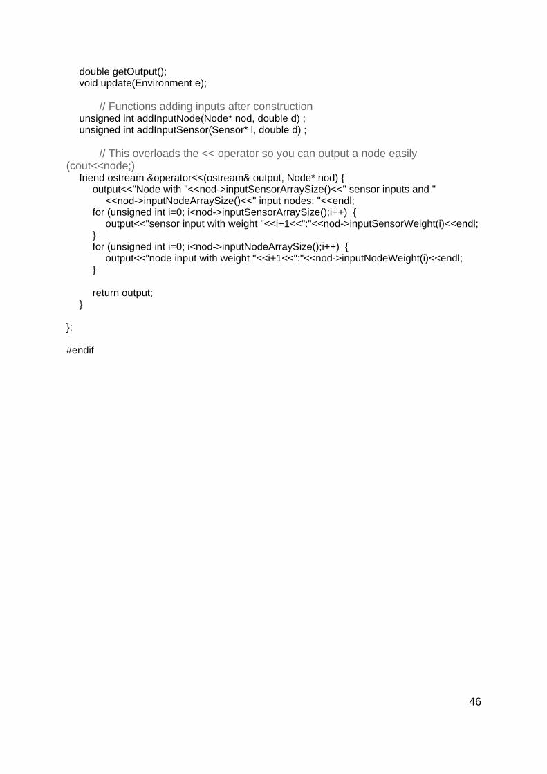
double getOutput();void update(Environment e);

// Functions adding inputs after construction unsigned int addInputNode(Node* nod, double d) ;unsigned int addInputSensor(Sensor* l, double d) ;

// This overloads the << operator so you can output a node easily(cout<<node;)

friend ostream &operator<<(ostream& output, Node* nod) {output<<"Node with "<<nod->inputSensorArraySize()<<" sensor inputs and "

<<nod->inputNodeArraySize()<<" input nodes: "<<endl;for (unsigned int i=0; i<nod->inputSensorArraySize();i++) {

output<<"sensor input with weight "<<i+1<<":"<<nod->inputSensorWeight(i)<<endl;}for (unsigned int i=0; i<nod->inputNodeArraySize();i++) {

output<<"node input with weight "<<i+1<<":"<<nod->inputNodeWeight(i)<<endl;}

return output;}

};

#endif

46

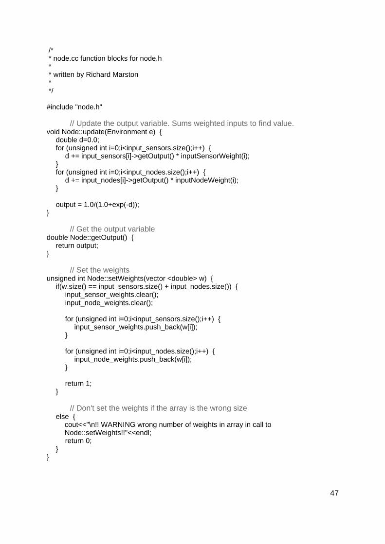
/* * node.cc function blocks for node.h * * written by Richard Marston * */

#include "node.h"

// Update the output variable. Sums weighted inputs to find value.void Node::update(Environment e) {

double d=0.0; for (unsigned int i=0;i<input_sensors.size();i++) {

d += input_sensors[i]->getOutput() * inputSensorWeight(i);}

for (unsigned int i=0;i<input_nodes.size();i++) {d += input_nodes[i]->getOutput() * inputNodeWeight(i);

}

output = 1.0/(1.0+exp(-d));}

// Get the output variabledouble Node::getOutput() {

return output;}

// Set the weightsunsigned int Node::setWeights(vector <double> w) {

if(w.size() == input_sensors.size() + input_nodes.size()) {input_sensor_weights.clear();input_node_weights.clear();

for (unsigned int i=0;i<input_sensors.size();i++) {input_sensor_weights.push_back(w[i]);

}

for (unsigned int i=0;i<input_nodes.size();i++) {input_node_weights.push_back(w[i]);

}

return 1;}

// Don't set the weights if the array is the wrong sizeelse {

cout<<"\n!! WARNING wrong number of weights in array in call to Node::setWeights!!"<<endl;return 0;

}}

47

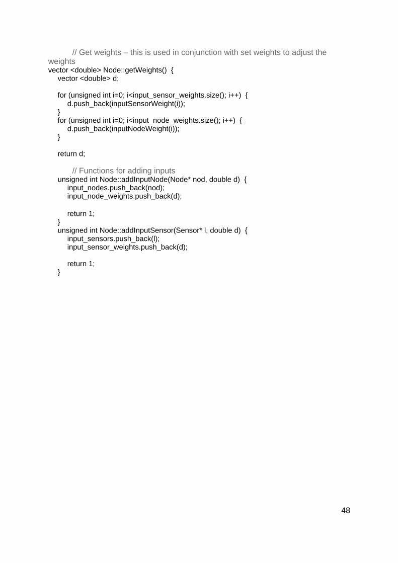
// Get weights – this is used in conjunction with set weights to adjust theweightsvector <double> Node::getWeights() {

vector <double> d;

for (unsigned int i=0; i<input_sensor_weights.size(); i++) {d.push_back(inputSensorWeight(i));

}for (unsigned int i=0; i<input_node_weights.size(); i++) {

d.push_back(inputNodeWeight(i));}

return d;

// Functions for adding inputsunsigned int Node::addInputNode(Node* nod, double d) {

input_nodes.push_back(nod); input_node_weights.push_back(d);

return 1;}unsigned int Node::addInputSensor(Sensor* l, double d) {

input_sensors.push_back(l); input_sensor_weights.push_back(d);

return 1;}

48

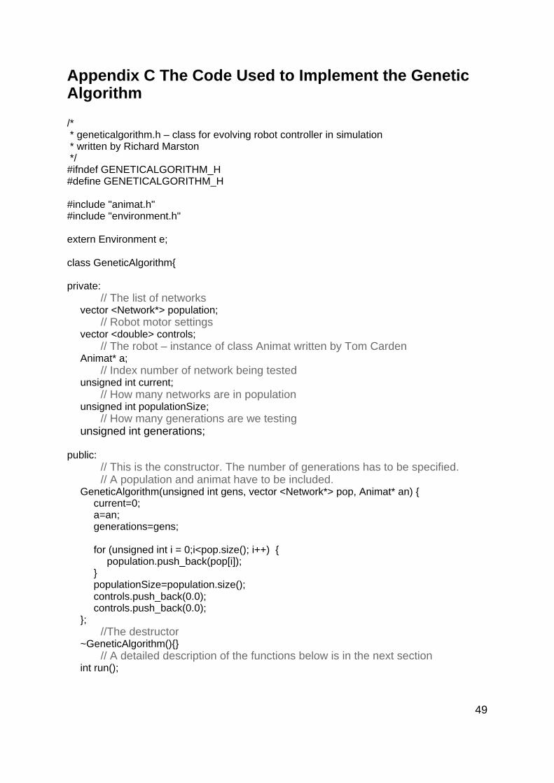
Appendix C The Code Used to Implement the GeneticAlgorithm

/* * geneticalgorithm.h – class for evolving robot controller in simulation * written by Richard Marston */#ifndef GENETICALGORITHM_H#define GENETICALGORITHM_H

#include "animat.h"#include "environment.h"

extern Environment e;

class GeneticAlgorithm{

private:// The list of networks

vector <Network*> population;// Robot motor settings

vector <double> controls;// The robot – instance of class Animat written by Tom Carden

Animat* a;// Index number of network being tested

unsigned int current;// How many networks are in population

unsigned int populationSize;// How many generations are we testing

unsigned int generations;

public:// This is the constructor. The number of generations has to be specified.

// A population and animat have to be included. GeneticAlgorithm(unsigned int gens, vector <Network*> pop, Animat* an) {

current=0;a=an;generations=gens;

for (unsigned int i = 0;i<pop.size(); i++) {population.push_back(pop[i]);

}populationSize=population.size();controls.push_back(0.0);controls.push_back(0.0);

};//The destructor

~GeneticAlgorithm(){}// A detailed description of the functions below is in the next section

int run();

49

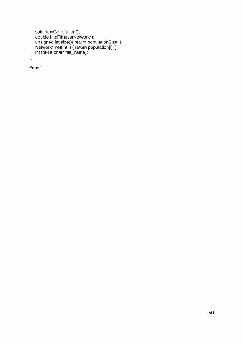
void nextGeneration();double findFitness(Network*);unsigned int size(){ return populationSize; }Network* net(int i) { return population[i]; }int toFile(char* file_name);

};

#endif

50

/* * geneticalgorithm.cc - function blocks for geneticalgorithm.h * written by Richard Marston */

#include "geneticalgorithm.h"#include <fstream>

// findFitness - this is the fitness functiondouble GeneticAlgorithm::findFitness(Network* gen) {

double x,y;double score=0.0;double elapsedTime=0.0;double timesteps=0.0;double distance,newdistance;

// This sets the robot's controller to the network we are testinga->controller=gen;

// Test each network 10 times in random locationsfor (int i=0;i<10;i++) {

elapsedTime=0.0;a->resetRandom();

while(elapsedTime <= p.timeLimit){

distance=1000.0;

// For each line pixel, calculate its' distance, and substitute it for thedistance to // the line if it is the closest one found yet.

for(int i=0;i<e.scenery[0]->getDataSize(); i++) {newdistance=sqrt((e.scenery[0]->getDataX(i)-x)*(e.scenery[0]->getDataX(i)-x) +(e.scenery[0]->getDataY(i)-y)*(e.scenery[0]->getDataY(i)-y));if(newdistance<distance) {

distance=newdistance;}

}

// Add the inverse of the distance to the line to the score// Networks near the line score more.

score+=1/distance;elapsedTime+=0.05;timesteps+=1.0;

// Update the robot's controlsa->controller->update(e);controls=a->controller->getOutput();

// This calculates the movement of the robot and works out if it has hitthe wall

51

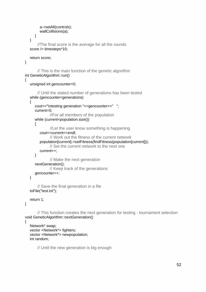
a->setAll(controls);wallCollisions(a);

}}

//The final score is the average for all the roundsscore /= timesteps*10;

return score;}

// This is the main function of the genetic algorithmint GeneticAlgorithm::run(){

unsigned int gencounter=0;

// Until the stated number of generations has been testedwhile (gencounter<generations){

cout<<"\ntesting generation "<<gencounter<<" ";current=0;

//For all members of the populationwhile (current<population.size()){

//Let the user know something is happeningcout<<current<<endl;

// Work out the fitness of the current networkpopulation[current]->setFitness(findFitness(population[current]));

// Set the current network to the next onecurrent++;

} // Make the next generation

nextGeneration();// Keep track of the generations

gencounter++;}

// Save the final generation in a filetoFile("test.txt");

return 1;}

// This function creates the next generation for testing - tournament selectionvoid GeneticAlgorithm::nextGeneration(){

Network* swap;vector <Network*> fighters;vector <Network*> newpopulation;int random;

// Until the new generation is big enough

52

for (unsigned int i=0;i<populationSize;i++){

// Do this as many times as should be in each tournament (twice in thiscase)

for(int j=0;j<2;j++){

// Select one of the population at random and put it in the fightersvector

random=(int)((double)population.size()*(double)rand()/RAND_MAX);fighters.push_back(population[random]);

// Sorting algorithm - makes sure fittest fighter is first in line - doesnothing if

// fighters.size() = 1 (if there is only one fighter)for (unsigned int k=fighters.size()-1;k>0;k--){

if (fighters[k]->getFitness() > fighters[k-1]->getFitness()){

swap=fighters[k-1];fighters[k-1]=fighters[k];fighters[k]=swap;

}else break;

}}

// put the fittest one into the new population and empty the fightervector for // the next go

newpopulation.push_back(fighters[0]);fighters.clear();

}

// Delete the old population and replace it with the newpopulation.clear();population=newpopulation;

// Everyone gets mutated by a random amount from 0-0.1for (unsigned int i=0;i<population.size();i++){

population[i]->mutate();}

}

// Function to write the final population to a fileint GeneticAlgorithm::toFile(char* file_name){

fstream outfile;

outfile.open (file_name, fstream::out);

for (unsigned int i=0;i<population.size();i++){

outfile << population[i];

53

}

outfile.close();return 1;

}

54