Embed Size (px)
Citation preview
R. Rojas: Neural Networks, Springer-Verlag, Berlin, 1996
Raul Rojas
Neural Networks
A Systematic Introduction
Springer
Berlin Heidelberg NewYork
HongKong London
Milan Paris Tokyo
R. Rojas: Neural Networks, Springer-Verlag, Berlin, 1996R. Rojas: Neural Networks, Springer-Verlag, Berlin, 1996R. Rojas: Neural Networks, Springer-Verlag, Berlin, 1996

R. Rojas: Neural Networks, Springer-Verlag, Berlin, 1996
V
R. Rojas: Neural Networks, Springer-Verlag, Berlin, 1996R. Rojas: Neural Networks, Springer-Verlag, Berlin, 1996R. Rojas: Neural Networks, Springer-Verlag, Berlin, 1996

R. Rojas: Neural Networks, Springer-Verlag, Berlin, 1996R. Rojas: Neural Networks, Springer-Verlag, Berlin, 1996R. Rojas: Neural Networks, Springer-Verlag, Berlin, 1996R. Rojas: Neural Networks, Springer-Verlag, Berlin, 1996
R. Rojas: Neural Networks, Springer-Verlag, Berlin, 1996
Foreword
One of the well-springs of mathematical inspiration has been the continu-ing attempt to formalize human thought. From the syllogisms of the Greeks,through all of logic and probability theory, cognitive models have led to beau-tiful mathematics and wide ranging application. But mental processes haveproven to be more complex than any of the formal theories and the variousidealizations have broken off to become separate fields of study and applica-tion.
It now appears that the same thing is happening with the recent devel-opments in connectionist and neural computation. Starting in the 1940s andwith great acceleration since the 1980s, there has been an effort to modelcognition using formalisms based on increasingly sophisticated models of thephysiology of neurons. Some branches of this work continue to focus on biolog-ical and psychological theory, but as in the past, the formalisms are taking ona mathematical and application life of their own. Several varieties of adaptivenetworks have proven to be practical in large difficult applied problems andthis has led to interest in their mathematical and computational properties.
We are now beginning to see good textbooks for introducing the subjectto various student groups. This book by Raul Rojas is aimed at advancedundergraduates in computer science and mathematics. This is a revised versionof his German text which has been quite successful. It is also a valuable self-instruction source for professionals interested in the relation of neural networkideas to theoretical computer science and articulating disciplines.
The book is divided into eighteen chapters, each designed to be taught inabout one week. The first eight chapters follow a progression and the laterones can be covered in a variety of orders. The emphasis throughout is onexplicating the computational nature of the structures and processes and re-lating them to other computational formalisms. Proofs are rigorous, but notoverly formal, and there is extensive use of geometric intuition and diagrams.Specific applications are discussed, with the emphasis on computational ratherthan engineering issues. There is a modest number of exercises at the end ofmost chapters.
R. Rojas: Neural Networks, Springer-Verlag, Berlin, 1996R. Rojas: Neural Networks, Springer-Verlag, Berlin, 1996R. Rojas: Neural Networks, Springer-Verlag, Berlin, 1996
R. Rojas: Neural Networks, Springer-Verlag, Berlin, 1996
VIII Foreword
The most widely applied mechanisms involve adapting weights in feed-forward networks of uniform differentiable units and these are covered thor-oughly. In addition to chapters on the background, fundamentals, and varia-tions on backpropagation techniques, there is treatment of related questionsfrom statistics and computational complexity.
There are also several chapters covering recurrent networks including thegeneral associative net and the models of Hopfield and Kohonen. Stochas-tic variants are presented and linked to statistical physics and Boltzmannlearning. Other chapters (weeks) are dedicated to fuzzy logic, modular neuralnetworks, genetic algorithms, and an overview of computer hardware devel-oped for neural computation. Each of the later chapters is self-contained andshould be readable by a student who has mastered the first half of the book.
The most remarkable aspect of neural computation at the present is thespeed at which it is maturing and becoming integrated with traditional disci-plines. This book is both an indication of this trend and a vehicle for bringingit to a generation of mathematically inclined students.
Berkeley, California Jerome Feldman
R. Rojas: Neural Networks, Springer-Verlag, Berlin, 1996R. Rojas: Neural Networks, Springer-Verlag, Berlin, 1996R. Rojas: Neural Networks, Springer-Verlag, Berlin, 1996
Preface
This book arose from my lectures on neural networks at the Free Universityof Berlin and later at the University of Halle. I started writing a new textout of dissatisfaction with the literature available at the time. Most bookson neural networks seemed to be chaotic collections of models and there wasno clear unifying theoretical thread connecting them. The results of my ef-forts were published in German by Springer-Verlag under the title Theorieder neuronalen Netze. I tried in that book to put the accent on a system-atic development of neural network theory and to stimulate the intuition ofthe reader by making use of many figures. Intuitive understanding fosters amore immediate grasp of the objects one studies, which stresses the concretemeaning of their relations. Since then some new books have appeared, whichare more systematic and comprehensive than those previously available, butI think that there is still much room for improvement. The German editionhas been quite successful and at the time of this writing it has gone throughfive printings in the space of three years.
However, this book is not a translation. I rewrote the text, added newsections, and deleted some others. The chapter on fast learning algorithms iscompletely new and some others have been adapted to deal with interestingadditional topics. The book has been written for undergraduates, and the onlymathematical tools needed are those which are learned during the first twoyears at university. The book offers enough material for a semester, althoughI do not normally go through all chapters. It is possible to omit some of themso as to spend more time on others. Some chapters from this book have beenused successfully for university courses in Germany, Austria, and the UnitedStates.
The various branches of neural networks theory are all interrelated closelyand quite often unexpectedly. Even so, because of the great diversity of thematerial treated, it was necessary to make each chapter more or less self-contained. There are a few minor repetitions but this renders each chapterunderstandable and interesting. There is considerable flexibility in the orderof presentation for a course. Chapter 1 discusses the biological motivation
R. Rojas: Neural Networks, Springer-Verlag, Berlin, 1996R. Rojas: Neural Networks, Springer-Verlag, Berlin, 1996
X Preface
of the whole enterprise. Chapters 2, 3, and 4 deal with the basics of thresh-old logic and should be considered as a unit. Chapter 5 introduces vectorquantization and unsupervised learning. Chapter 6 gives a nice geometricalinterpretation of perceptron learning. Those interested in stressing currentapplications of neural networks can skip Chapters 5 and 6 and go directlyto the backpropagation algorithm (Chapter 7). I am especially proud of thischapter because it introduces backpropagation with minimal effort, using agraphical approach, yet the result is more general than the usual derivationsof the algorithm in other books. I was rather surprised to see that NeuralComputation published in 1996 a paper about what is essentially the methodcontained in my German book of 1993.
Those interested in statistics and complexity theory should review Chap-ters 9 and 10. Chapter 11 is an intermezzo and clarifies the relation betweenfuzzy logic and neural networks. Recurrent networks are handled in the threechapters, dealing respectively with associative memories, the Hopfield model,and Boltzmann machines. They should be also considered a unit. The bookcloses with a review of self-organization and evolutionary methods, followedby a short survey of currently available hardware for neural networks.
We are still struggling with neural network theory, trying to find a moresystematic and comprehensive approach. Every chapter should convey to thereader an understanding of one small additional piece of the larger picture. Isometimes compare the current state of the theory with a big puzzle which weare all trying to put together. This explains the small puzzle pieces that thereader will find at the end of each chapter. Enough discussion – Let us startour journey into the fascinating world of artificial neural networks withoutfurther delay.
Errata and electronic information
This book has an Internet home page. Any errors reported by readers, newideas, and suggested exercises can be downloaded from Berlin, Germany. TheWWW link is: http://www.inf.fu-berlin.de/∼rojas/neural. The home pageoffers also some additional useful information about neural networks. You cansend your comments by e-mail to [email protected].
Acknowledgements
Many friends and colleagues have contributed to the quality of this book.The names of some of them are listed in the preface to the German edition of1993. Phil Maher, Rosi Weinert-Knapp, and Gaye Rochow revised my originalmanuscript. Andrew J. Ross, English editor at Springer-Verlag in Heidelberg,took great care in degermanizing my linguistic constructions.
The book was written at three different institutions: The Free Universityof Berlin provided an ideal working environment during the first phase of writ-ing. Vilim Vesligaj configured TeX so that it would accept Springer’s style.
R. Rojas: Neural Networks, Springer-Verlag, Berlin, 1996R. Rojas: Neural Networks, Springer-Verlag, Berlin, 1996
Preface XI
Gunter Feuer, Marcus Pfister, Willi Wolf, and Birgit Muller were patient dis-cussion partners. I had many discussions with Frank Darius on damned liesand statistics. The work was finished at Halle’s Martin Luther University. Mycollaborator Bernhard Frotschl and some of my students found many of myearly TeX-typos. I profited from two visits to the International Computer Sci-ence Institute in Berkeley during the summers of 1994 and 1995. I especiallythank Jerry Feldman, Joachim Beer, and Nelson Morgan for their encour-agement. Lokendra Shastri tested the backpropagation chapter “in the field”,that is in his course on connectionist models at UC Berkeley. It was very re-warding to spend the evenings talking to Andres and Celina Albanese aboutother kinds of networks (namely real computer networks). Lotfi Zadeh wasvery kind in inviting me to present my visualization methods at his Semi-nar on Soft Computing. Due to the efforts of Dieter Ernst there is no goodrestaurant in the Bay Area where I have not been.
It has been a pleasure working with Springer-Verlag and the head of theplanning section, Dr. Hans Wossner, in the development of this text. Withhim cheering from Heidelberg I could survive the whole ordeal of TeXing morethan 500 pages.
Finally, I thank my daughter Tania and my wife Margarita Esponda fortheir love and support during the writing of this book. Since my Germanbook was dedicated to Margarita, the new English edition is now dedicatedto Tania. I really hope she will read this book in the future (and I hope shewill like it).
Berlin and Halle Raul Rojas GonzalezMarch 1996
R. Rojas: Neural Networks, Springer-Verlag, Berlin, 1996R. Rojas: Neural Networks, Springer-Verlag, Berlin, 1996
“For Reason, in this sense, is nothing butReckoning (that is, Adding and Subtracting).”
Thomas Hobbes, Leviathan.
R. Rojas: Neural Networks, Springer-Verlag, Berlin, 1996R. Rojas: Neural Networks, Springer-Verlag, Berlin, 1996

R. Rojas: Neural Networks, Springer-Verlag, Berlin, 1996R. Rojas: Neural Networks, Springer-Verlag, Berlin, 1996
R. Rojas: Neural Networks, Springer-Verlag, Berlin, 1996
1
The Biological Paradigm
1.1 Neural computation
Research in the field of neural networks has been attracting increasing atten-tion in recent years. Since 1943, when Warren McCulloch and Walter Pittspresented the first model of artificial neurons, new and more sophisticatedproposals have been made from decade to decade. Mathematical analysis hassolved some of the mysteries posed by the new models but has left many ques-tions open for future investigations. Needless to say, the study of neurons, theirinterconnections, and their role as the brain’s elementary building blocks isone of the most dynamic and important research fields in modern biology. Wecan illustrate the relevance of this endeavor by pointing out that between 1901and 1991 approximately ten percent of the Nobel Prizes for Physiology andMedicine were awarded to scientists who contributed to the understanding ofthe brain. It is not an exaggeration to say that we have learned more aboutthe nervous system in the last fifty years than ever before.
In this book we deal with artificial neural networks, and therefore the firstquestion to be clarified is their relation to the biological paradigm. What do weabstract from real neurons for our models? What is the link between neuronsand artificial computing units? This chapter gives a preliminary answer tothese important questions.
1.1.1 Natural and artificial neural networks
Artificial neural networks are an attempt at modeling the information pro-cessing capabilities of nervous systems. Thus, first of all, we need to considerthe essential properties of biological neural networks from the viewpoint of in-formation processing. This will allow us to design abstract models of artificialneural networks, which can then be simulated and analyzed.
Although the models which have been proposed to explain the structureof the brain and the nervous systems of some animals are different in many
R. Rojas: Neural Networks, Springer-Verlag, Berlin, 1996R. Rojas: Neural Networks, Springer-Verlag, Berlin, 1996
R. Rojas: Neural Networks, Springer-Verlag, Berlin, 1996
4 1 The Biological Paradigm
respects, there is a general consensus that the essence of the operation ofneural ensembles is “control through communication” [72]. Animal nervoussystems are composed of thousands or millions of interconnected cells. Eachone of them is a very complex arrangement which deals with incoming signalsin many different ways. However, neurons are rather slow when compared toelectronic logic gates. These can achieve switching times of a few nanoseconds,whereas neurons need several milliseconds to react to a stimulus. Neverthelessthe brain is capable of solving problems which no digital computer can yetefficiently deal with.
Massive and hierarchical networking of the brain seems to be the funda-mental precondition for the emergence of consciousness and complex behav-ior [202]. So far, however, biologists and neurologists have concentrated theirresearch on uncovering the properties of individual neurons. Today, the mech-anisms for the production and transport of signals from one neuron to theother are well-understood physiological phenomena, but how these individualsystems cooperate to form complex and massively parallel systems capableof incredible information processing feats has not yet been completely elu-cidated. Mathematics, physics, and computer science can provide invaluablehelp in the study of these complex systems. It is not surprising that the studyof the brain has become one of the most interdisciplinary areas of scientificresearch in recent years.
However, we should be careful with the metaphors and paradigms com-monly introduced when dealing with the nervous system. It seems to be aconstant in the history of science that the brain has always been comparedto the most complicated contemporary artifact produced by human industry[297]. In ancient times the brain was compared to a pneumatic machine, inthe Renaissance to a clockwork, and at the end of the last century to the tele-phone network. There are some today who consider computers the paradigmpar excellence of a nervous system. It is rather paradoxical that when Johnvon Neumann wrote his classical description of future universal computers, hetried to choose terms that would describe computers in terms of brains, notbrains in terms of computers.
The nervous system of an animal is an information processing totality. Thesensory inputs, i.e., signals from the environment, are coded and processedto evoke the appropriate response. Biological neural networks are just oneof many possible solutions to the problem of processing information. Themain difference between neural networks and conventional computer systemsis the massive parallelism and redundancy which they exploit in order to dealwith the unreliability of the individual computing units. Moreover, biologicalneural networks are self-organizing systems and each individual neuron is alsoa delicate self-organizing structure capable of processing information in manydifferent ways.
In this book we study the information processing capabilities of complexhierarchical networks of simple computing units. We deal with systems whosestructure is only partially predetermined. Some parameters modify the ca-
R. Rojas: Neural Networks, Springer-Verlag, Berlin, 1996R. Rojas: Neural Networks, Springer-Verlag, Berlin, 1996
R. Rojas: Neural Networks, Springer-Verlag, Berlin, 1996
1.1 Neural computation 5
pabilities of the network and it is our task to find the best combination forthe solution of a given problem. The adjustment of the parameters will bedone through a learning algorithm, i.e., not through explicit programmingbut through an automatic adaptive method.
A cursory review of the relevant literature on artificial neural networksleaves the impression of a chaotic mixture of very different network topologiesand learning algorithms. Commercial neural network simulators sometimesoffer several dozens of possible models. The large number of proposals hasled to a situation in which each single model appears as part of a big puzzlewhereas the bigger picture is absent. Consequently, in the following chapterswe try to solve this puzzle by systematically introducing and discussing eachof the neural network models in relation to the others.
Our approach consists of stating and answering the following questions:what information processing capabilities emerge in hierarchical systems ofprimitive computing units? What can be computed with these networks? Howcan these networks determine their structure in a self-organizing manner?
We start by considering biological systems. Artificial neural networks havearoused so much interest in recent years, not only because they exhibit inter-esting properties, but also because they try to mirror the kind of informationprocessing capabilities of nervous systems. Since information processing con-sists of transforming signals, we deal with the biological mechanisms for theirgeneration and transmission in this chapter. We discuss those biological pro-cesses by which neurons produce signals, and absorb and modify them in orderto retransmit the result. In this way biological neural networks give us a clueregarding the properties which would be interesting to include in our artificialnetworks.
1.1.2 Models of computation
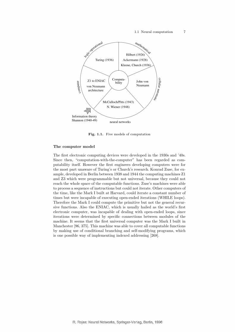
Artificial neural networks can be considered as just another approach to theproblem of computation. The first formal definitions of computability wereproposed in the 1930s and ’40s and at least five different alternatives werestudied at the time. The computer era was started, not with one single ap-proach, but with a contest of alternative computing models. We all know thatthe von Neumann computer emerged as the undisputed winner in this con-frontation, but its triumph did not lead to the dismissal of the other computingmodels. Figure 1.1 shows the five principal contenders:
The mathematical model
Mathematicians avoided dealing with the problem of a function’s computabil-ity until the beginning of this century. This happened not just because exis-tence theorems were considered sufficient to deal with functions, but mainlybecause nobody had come up with a satisfactory definition of computability,certainly a relative concept which depends on the specific tools that can be
R. Rojas: Neural Networks, Springer-Verlag, Berlin, 1996R. Rojas: Neural Networks, Springer-Verlag, Berlin, 1996
R. Rojas: Neural Networks, Springer-Verlag, Berlin, 1996
6 1 The Biological Paradigm
used. The general solution for algebraic equations of degree five, for example,cannot be formulated using only algebraic functions, yet this can be done ifa more general class of functions is allowed as computational primitives. Thesquaring of the circle, to give another example, is impossible using ruler andcompass, but it has a trivial real solution.
If we want to talk about computability we must therefore specify whichtools are available. We can start with the idea that some primitive functionsand composition rules are “obviously” computable. All other functions whichcan be expressed in terms of these primitives and composition rules are thenalso computable.
David Hilbert, the famous German mathematician, was the first to statethe conjecture that a certain class of functions contains all intuitively com-putable functions. Hilbert was referring to the primitive recursive functions,the class of functions which can be constructed from the zero and successorfunction using composition, projection, and a deterministic number of itera-tions (primitive recursion). However, in 1928, Wilhelm Ackermann was ableto find a computable function which is not primitive recursive. This led tothe definition of the general recursive functions [154]. In this formalism, anew composition rule has to be introduced, the so-called µ operator, which isequivalent to an indeterminate recursion or a lookup in an infinite table. Atthe same time Alonzo Church and collaborators developed the lambda calcu-lus, another alternative to the mathematical definition of the computabilityconcept [380]. In 1936, Church and Kleene were able to show that the generalrecursive functions can be expressed in the formalism of the lambda calculus.This led to the Church thesis that computable functions are the general recur-sive functions. David Deutsch has recently added that this thesis should beconsidered to be a statement about the physical world and be given the samestatus as a physical principle. He thus speaks of a “Church principle” [109].
The logic-operational model (Turing machines)
In his classical paper “On Computable Numbers with an Application to theEntscheidungsproblem” Alan Turing introduced another kind of computingmodel. The advantage of his approach is that it consists in an operational,mechanical model of computability. A Turing machine is composed of an infi-nite tape, in which symbols can be stored and read again. A read-write headcan move to the left or to the right according to its internal state, whichis updated at each step. The Turing thesis states that computable functionsare those which can be computed with this kind of device. It was formulatedconcurrently with the Church thesis and Turing was able to show almost im-mediately that they are equivalent [435]. The Turing approach made clear forthe first time what “programming” means, curiously enough at a time whenno computer had yet been built.
R. Rojas: Neural Networks, Springer-Verlag, Berlin, 1996R. Rojas: Neural Networks, Springer-Verlag, Berlin, 1996
R. Rojas: Neural Networks, Springer-Verlag, Berlin, 1996
1.1 Neural computation 7
com
pute
r
logi
c-op
erati
onal
neural networks
Hilbert (1926)
Ackermann (1928)
Kleene, Church (1936)
Turing (1936)
Computa-bility
Z1 to ENIAC
von Neumann
architecture
John von
Neumann
McCulloch/Pitts (1943)
N. Wiener (1948)
Information theory
Shannon (1940-49)
mathematical
cellu
lar
auto
mata
Fig. 1.1. Five models of computation
The computer model
The first electronic computing devices were developed in the 1930s and ’40s.Since then, “computation-with-the-computer” has been regarded as com-putability itself. However the first engineers developing computers were forthe most part unaware of Turing’s or Church’s research. Konrad Zuse, for ex-ample, developed in Berlin between 1938 and 1944 the computing machines Z1and Z3 which were programmable but not universal, because they could notreach the whole space of the computable functions. Zuse’s machines were ableto process a sequence of instructions but could not iterate. Other computers ofthe time, like the Mark I built at Harvard, could iterate a constant number oftimes but were incapable of executing open-ended iterations (WHILE loops).Therefore the Mark I could compute the primitive but not the general recur-sive functions. Also the ENIAC, which is usually hailed as the world’s firstelectronic computer, was incapable of dealing with open-ended loops, sinceiterations were determined by specific connections between modules of themachine. It seems that the first universal computer was the Mark I built inManchester [96, 375]. This machine was able to cover all computable functionsby making use of conditional branching and self-modifying programs, whichis one possible way of implementing indexed addressing [268].
R. Rojas: Neural Networks, Springer-Verlag, Berlin, 1996R. Rojas: Neural Networks, Springer-Verlag, Berlin, 1996
R. Rojas: Neural Networks, Springer-Verlag, Berlin, 1996
8 1 The Biological Paradigm
Cellular automata
The history of the development of the first mechanical and electronic comput-ing devices shows how difficult it was to reach a consensus on the architectureof universal computers. Aspects such as the economy or the dependability ofthe building blocks played a role in the discussion, but the main problem wasthe definition of the minimal architecture needed for universality. In machineslike the Mark I and the ENIAC there was no clear separation between memoryand processor, and both functional elements were intertwined. Some machinesstill worked with base 10 and not 2, some were sequential and others parallel.
John von Neumann, who played a major role in defining the architecture ofsequential machines, analyzed at that time a new computational model whichhe called cellular automata. Such automata operate in a “computing space” inwhich all data can be processed simultaneously. The main problem for cellularautomata is communication and coordination between all the computing cells.This can be guaranteed through certain algorithms and conventions. It is notdifficult to show that all computable functions, in the sense of Turing, canalso be computed with cellular automata, even of the one-dimensional type,possessing only a few states. Turing himself considered this kind of computingmodel at one point in his career [192].
Cellular automata as computing model resemble massively parallel multi-processor systems of the kind that has attracted considerable interest recently.
The biological model (neural networks)
The explanation of important aspects of the physiology of neurons set thestage for the formulation of artificial neural network models which do not op-erate sequentially, as Turing machines do. Neural networks have a hierarchicalmultilayered structure which sets them apart from cellular automata, so thatinformation is transmitted not only to the immediate neighbors but also tomore distant units. In artificial neural networks one can connect each unitto any other. In contrast to conventional computers, no program is handedover to the hardware – such a program has to be created, that is, the freeparameters of the network have to be found adaptively.
Although neural networks and cellular automata are potentially more effi-cient than conventional computers in certain application areas, at the time oftheir conception they were not yet ready to take center stage. The necessarytheory for harnessing the dynamics of complex parallel systems is still be-ing developed right before our eyes. In the meantime, conventional computertechnology has made great strides.
There is no better illustration for the simultaneous and related emergenceof these various computability models than the life and work of John vonNeumann himself. He participated in the definition and development of atleast three of these models: in the architecture of sequential computers [417],
R. Rojas: Neural Networks, Springer-Verlag, Berlin, 1996R. Rojas: Neural Networks, Springer-Verlag, Berlin, 1996
R. Rojas: Neural Networks, Springer-Verlag, Berlin, 1996
1.2 Networks of neurons 9
the theory of cellular automata and the first neural network models. He alsocollaborated with Church and Turing in Princeton [192].
Artificial neural networks have, as initial motivation, the structure of bi-ological systems, and constitute an alternative computability paradigm. Forthat reason we will review some aspects of the way in which biological sys-tems perform information processing. The fascination which still pervadesthis research field has much to do with the points of contact with the sur-prisingly elegant methods used by neurons in order to process information atthe cellular level. Several million years of evolution have led to very sophis-ticated solutions to the problem of dealing with an uncertain environment.In this chapter we will discuss some elements of these strategies in order todetermine what features we want to adopt in our abstract models of neuralnetworks.
1.1.3 Elements of a computing model
What are the elementary components of any conceivable computing model?In the theory of general recursive functions, for example, it is possible toreduce any computable function to some composition rules and a small set ofprimitive functions. For a universal computer, we ask about the existence of aminimal and sufficient instruction set. For an arbitrary computing model thefollowing metaphoric expression has been proposed:
computation = storage+ transmission+ processing.
The mechanical computation of a function presupposes that these threeelements are present, that is, that data can be stored, communicated to thefunctional units of the model and transformed. It is implicitly assumed that acertain coding of the data has been agreed upon. Coding plays an importantrole in information processing because, as Claude Shannon showed in 1948,when noise is present information can still be transmitted without loss, if theright code with the right amount of redundancy is chosen.
Modern computers transform storage of information into a form of infor-mation transmission. Static memory chips store a bit as a circulating currentuntil the bit is read. Turing machines store information in an infinite tape,whereas transmission is performed by the read-write head. Cellular automatastore information in each cell, which at the same time is a small processor.
1.2 Networks of neurons
In biological neural networks information is stored at the contact points be-tween different neurons, the so-called synapses. Later we will discuss what rolethese elements play for the storage, transmission, and processing of informa-tion. Other forms of storage are also known, because neurons are themselves
R. Rojas: Neural Networks, Springer-Verlag, Berlin, 1996R. Rojas: Neural Networks, Springer-Verlag, Berlin, 1996
R. Rojas: Neural Networks, Springer-Verlag, Berlin, 1996
10 1 The Biological Paradigm
complex systems of self-organizing signaling. In the next few pages we can-not do justice to all this complexity, but we analyze the most salient featuresand, with the metaphoric expression given above in mind, we will ask: howdo neurons compute?
1.2.1 Structure of the neurons
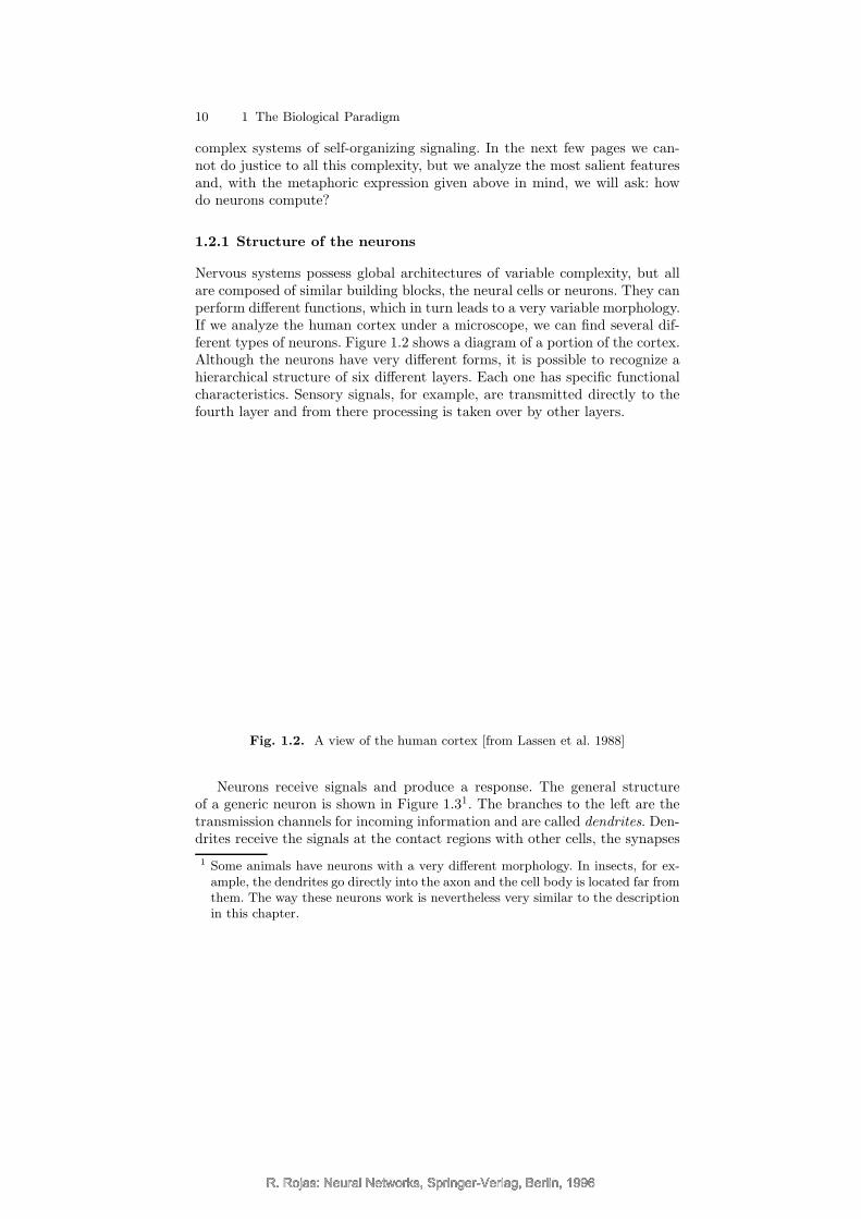
Nervous systems possess global architectures of variable complexity, but allare composed of similar building blocks, the neural cells or neurons. They canperform different functions, which in turn leads to a very variable morphology.If we analyze the human cortex under a microscope, we can find several dif-ferent types of neurons. Figure 1.2 shows a diagram of a portion of the cortex.Although the neurons have very different forms, it is possible to recognize ahierarchical structure of six different layers. Each one has specific functionalcharacteristics. Sensory signals, for example, are transmitted directly to thefourth layer and from there processing is taken over by other layers.
Fig. 1.2. A view of the human cortex [from Lassen et al. 1988]
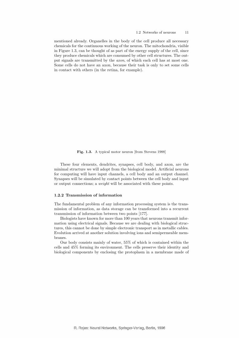
Neurons receive signals and produce a response. The general structureof a generic neuron is shown in Figure 1.31. The branches to the left are thetransmission channels for incoming information and are called dendrites. Den-drites receive the signals at the contact regions with other cells, the synapses
1 Some animals have neurons with a very different morphology. In insects, for ex-ample, the dendrites go directly into the axon and the cell body is located far fromthem. The way these neurons work is nevertheless very similar to the descriptionin this chapter.
R. Rojas: Neural Networks, Springer-Verlag, Berlin, 1996R. Rojas: Neural Networks, Springer-Verlag, Berlin, 1996
R. Rojas: Neural Networks, Springer-Verlag, Berlin, 1996
1.2 Networks of neurons 11
mentioned already. Organelles in the body of the cell produce all necessarychemicals for the continuous working of the neuron. The mitochondria, visiblein Figure 1.3, can be thought of as part of the energy supply of the cell, sincethey produce chemicals which are consumed by other cell structures. The out-put signals are transmitted by the axon, of which each cell has at most one.Some cells do not have an axon, because their task is only to set some cellsin contact with others (in the retina, for example).
Fig. 1.3. A typical motor neuron [from Stevens 1988]
These four elements, dendrites, synapses, cell body, and axon, are theminimal structure we will adopt from the biological model. Artificial neuronsfor computing will have input channels, a cell body and an output channel.Synapses will be simulated by contact points between the cell body and inputor output connections; a weight will be associated with these points.
1.2.2 Transmission of information
The fundamental problem of any information processing system is the trans-mission of information, as data storage can be transformed into a recurrenttransmission of information between two points [177].
Biologists have known for more than 100 years that neurons transmit infor-mation using electrical signals. Because we are dealing with biological struc-tures, this cannot be done by simple electronic transport as in metallic cables.Evolution arrived at another solution involving ions and semipermeable mem-branes.
Our body consists mainly of water, 55% of which is contained within thecells and 45% forming its environment. The cells preserve their identity andbiological components by enclosing the protoplasm in a membrane made of
R. Rojas: Neural Networks, Springer-Verlag, Berlin, 1996R. Rojas: Neural Networks, Springer-Verlag, Berlin, 1996
R. Rojas: Neural Networks, Springer-Verlag, Berlin, 1996
12 1 The Biological Paradigm
a double layer of molecules that form a diffusion barrier. Some salts, presentin our body, dissolve in the intracellular and extracellular fluid and dissociateinto negative and positive ions. Sodium chloride, for example, dissociates intopositive sodium ions (Na+) and negative chlorine ions (Cl−). Other positiveions present in the interior or exterior of the cells are potassium (K+) andcalcium (Ca2+). The membranes of the cells exhibit different degrees of per-meability for each one of these ions. The permeability is determined by thenumber and size of pores in the membrane, the so-called ionic channels. Theseare macromolecules with forms and charges which allow only certain ions togo from one side of the cell membrane to the other. Channels are selectivelypermeable to sodium, potassium or calcium ions. The specific permeabilityof the membrane leads to different distributions of ions in the interior andthe exterior of the cells and this, in turn, to the interior of neurons beingnegatively charged with respect to the extracellular fluid.
diffusion force diffusion forceelectrostatic
force
membrane
positive
ions
negative
ions
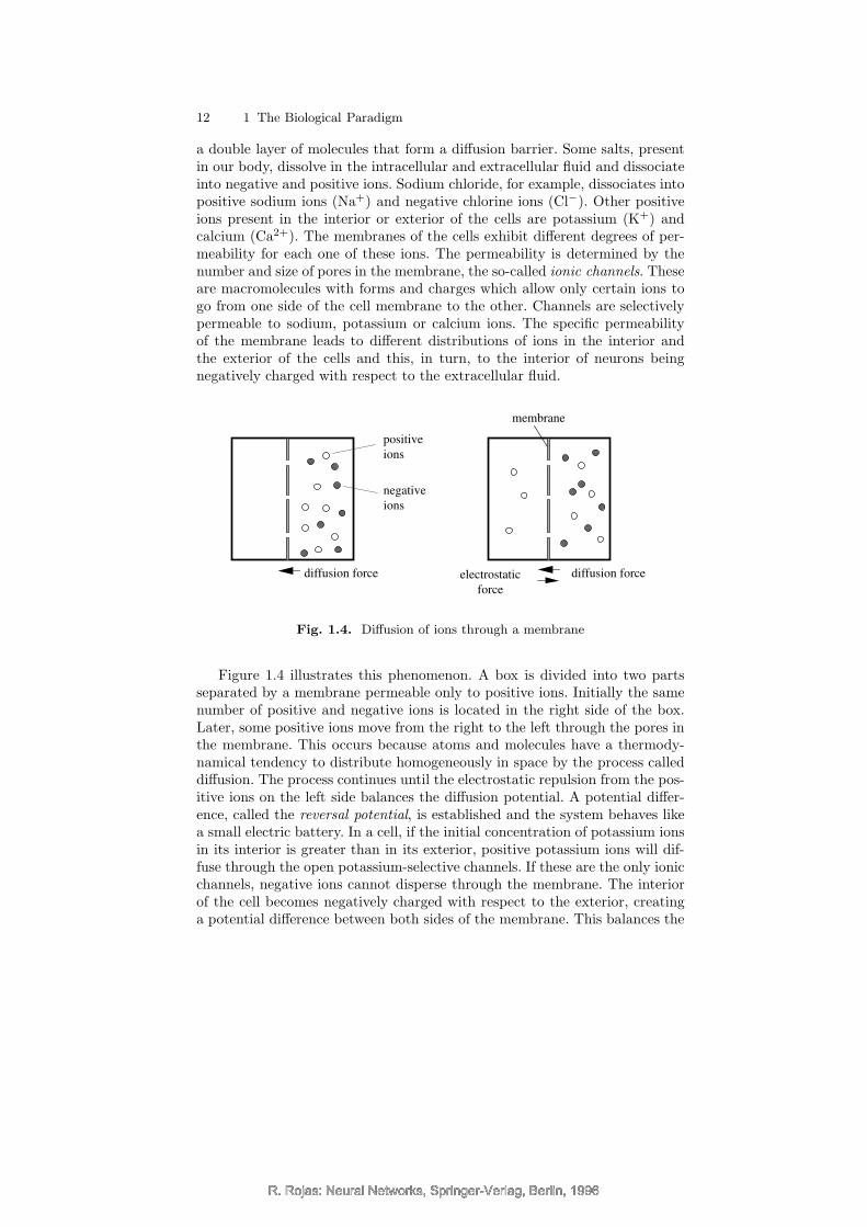
Fig. 1.4. Diffusion of ions through a membrane
Figure 1.4 illustrates this phenomenon. A box is divided into two partsseparated by a membrane permeable only to positive ions. Initially the samenumber of positive and negative ions is located in the right side of the box.Later, some positive ions move from the right to the left through the pores inthe membrane. This occurs because atoms and molecules have a thermody-namical tendency to distribute homogeneously in space by the process calleddiffusion. The process continues until the electrostatic repulsion from the pos-itive ions on the left side balances the diffusion potential. A potential differ-ence, called the reversal potential, is established and the system behaves likea small electric battery. In a cell, if the initial concentration of potassium ionsin its interior is greater than in its exterior, positive potassium ions will dif-fuse through the open potassium-selective channels. If these are the only ionicchannels, negative ions cannot disperse through the membrane. The interiorof the cell becomes negatively charged with respect to the exterior, creatinga potential difference between both sides of the membrane. This balances the
R. Rojas: Neural Networks, Springer-Verlag, Berlin, 1996R. Rojas: Neural Networks, Springer-Verlag, Berlin, 1996
R. Rojas: Neural Networks, Springer-Verlag, Berlin, 1996
1.2 Networks of neurons 13
diffusion potential, and, at some point, the net flow of potassium ions throughthe membrane falls to zero. The system reaches a steady state. The potentialdifference E for one kind of ion is given by the Nernst formula
E = k(ln(co)− ln(ci))
where ci is the concentration inside the cell, co the concentration in the ex-tracellular fluid and k is a proportionality constant [295]. For potassium ionsthe equilibrium potential is −80 mV.
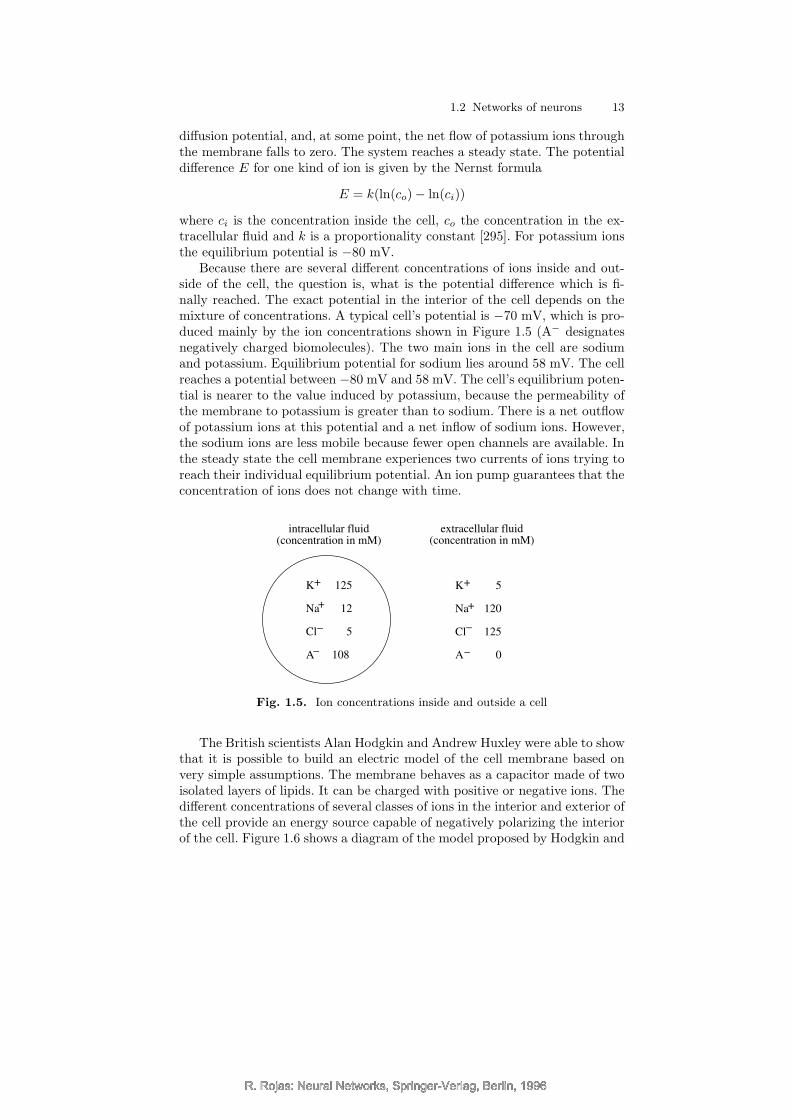
Because there are several different concentrations of ions inside and out-side of the cell, the question is, what is the potential difference which is fi-nally reached. The exact potential in the interior of the cell depends on themixture of concentrations. A typical cell’s potential is −70 mV, which is pro-duced mainly by the ion concentrations shown in Figure 1.5 (A− designatesnegatively charged biomolecules). The two main ions in the cell are sodiumand potassium. Equilibrium potential for sodium lies around 58 mV. The cellreaches a potential between −80 mV and 58 mV. The cell’s equilibrium poten-tial is nearer to the value induced by potassium, because the permeability ofthe membrane to potassium is greater than to sodium. There is a net outflowof potassium ions at this potential and a net inflow of sodium ions. However,the sodium ions are less mobile because fewer open channels are available. Inthe steady state the cell membrane experiences two currents of ions trying toreach their individual equilibrium potential. An ion pump guarantees that theconcentration of ions does not change with time.
extracellular fluid(concentration in mM)
intracellular fluid(concentration in mM)
K 5
Na 120
Cl 125
A 0
–
+
+
–
K 125
Na 12
Cl 5
A 108
+
–
–
+
Fig. 1.5. Ion concentrations inside and outside a cell
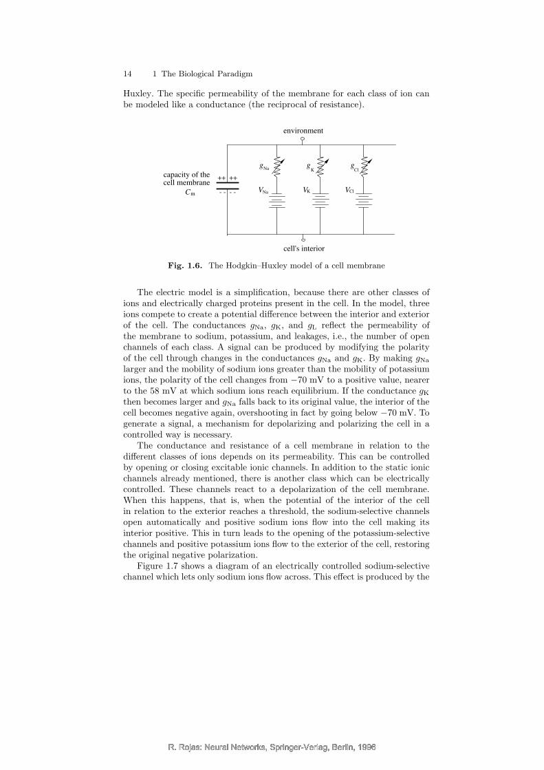
The British scientists Alan Hodgkin and Andrew Huxley were able to showthat it is possible to build an electric model of the cell membrane based onvery simple assumptions. The membrane behaves as a capacitor made of twoisolated layers of lipids. It can be charged with positive or negative ions. Thedifferent concentrations of several classes of ions in the interior and exterior ofthe cell provide an energy source capable of negatively polarizing the interiorof the cell. Figure 1.6 shows a diagram of the model proposed by Hodgkin and
R. Rojas: Neural Networks, Springer-Verlag, Berlin, 1996R. Rojas: Neural Networks, Springer-Verlag, Berlin, 1996
R. Rojas: Neural Networks, Springer-Verlag, Berlin, 1996
14 1 The Biological Paradigm
Huxley. The specific permeability of the membrane for each class of ion canbe modeled like a conductance (the reciprocal of resistance).
- - - -
++ ++
gNa
gK
gCl
environment
cell's interior
capacity of thecell membrane
CmV V VNa K Cl
Fig. 1.6. The Hodgkin–Huxley model of a cell membrane
The electric model is a simplification, because there are other classes ofions and electrically charged proteins present in the cell. In the model, threeions compete to create a potential difference between the interior and exteriorof the cell. The conductances gNa, gK, and gL reflect the permeability ofthe membrane to sodium, potassium, and leakages, i.e., the number of openchannels of each class. A signal can be produced by modifying the polarityof the cell through changes in the conductances gNa and gK. By making gNa
larger and the mobility of sodium ions greater than the mobility of potassiumions, the polarity of the cell changes from −70 mV to a positive value, nearerto the 58 mV at which sodium ions reach equilibrium. If the conductance gKthen becomes larger and gNa falls back to its original value, the interior of thecell becomes negative again, overshooting in fact by going below −70 mV. Togenerate a signal, a mechanism for depolarizing and polarizing the cell in acontrolled way is necessary.
The conductance and resistance of a cell membrane in relation to thedifferent classes of ions depends on its permeability. This can be controlledby opening or closing excitable ionic channels. In addition to the static ionicchannels already mentioned, there is another class which can be electricallycontrolled. These channels react to a depolarization of the cell membrane.When this happens, that is, when the potential of the interior of the cellin relation to the exterior reaches a threshold, the sodium-selective channelsopen automatically and positive sodium ions flow into the cell making itsinterior positive. This in turn leads to the opening of the potassium-selectivechannels and positive potassium ions flow to the exterior of the cell, restoringthe original negative polarization.
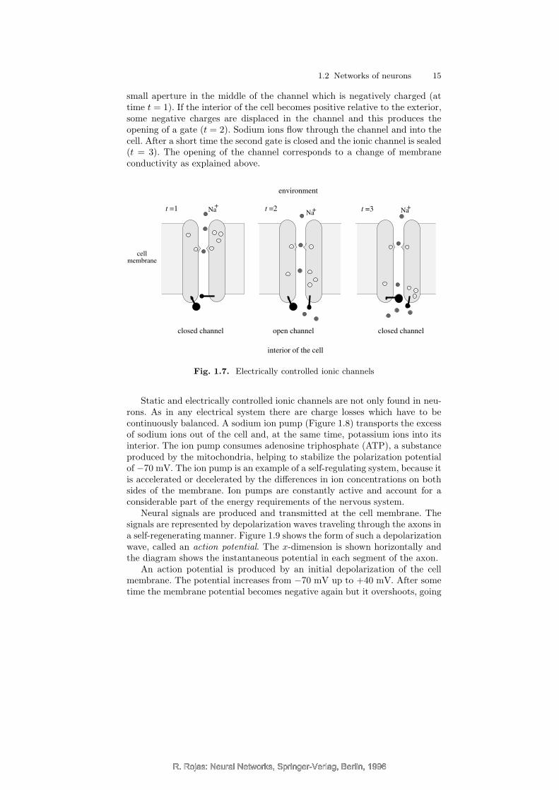
Figure 1.7 shows a diagram of an electrically controlled sodium-selectivechannel which lets only sodium ions flow across. This effect is produced by the
R. Rojas: Neural Networks, Springer-Verlag, Berlin, 1996R. Rojas: Neural Networks, Springer-Verlag, Berlin, 1996
R. Rojas: Neural Networks, Springer-Verlag, Berlin, 1996
1.2 Networks of neurons 15
small aperture in the middle of the channel which is negatively charged (attime t = 1). If the interior of the cell becomes positive relative to the exterior,some negative charges are displaced in the channel and this produces theopening of a gate (t = 2). Sodium ions flow through the channel and into thecell. After a short time the second gate is closed and the ionic channel is sealed(t = 3). The opening of the channel corresponds to a change of membraneconductivity as explained above.
cellmembrane
Na+
Na+ Na+
environment
closed channel closed channelopen channel
interior of the cell
t =1 t =2 t =3
Fig. 1.7. Electrically controlled ionic channels
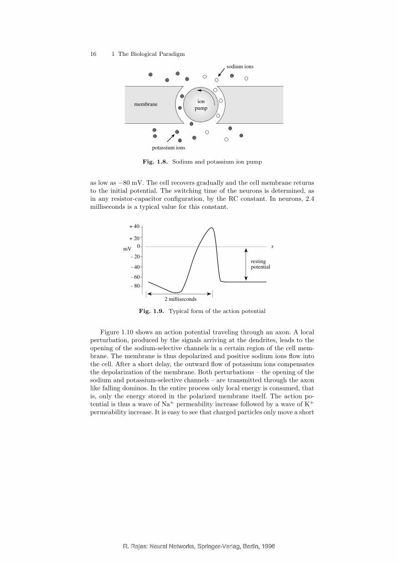
Static and electrically controlled ionic channels are not only found in neu-rons. As in any electrical system there are charge losses which have to becontinuously balanced. A sodium ion pump (Figure 1.8) transports the excessof sodium ions out of the cell and, at the same time, potassium ions into itsinterior. The ion pump consumes adenosine triphosphate (ATP), a substanceproduced by the mitochondria, helping to stabilize the polarization potentialof −70 mV. The ion pump is an example of a self-regulating system, because itis accelerated or decelerated by the differences in ion concentrations on bothsides of the membrane. Ion pumps are constantly active and account for aconsiderable part of the energy requirements of the nervous system.
Neural signals are produced and transmitted at the cell membrane. Thesignals are represented by depolarization waves traveling through the axons ina self-regenerating manner. Figure 1.9 shows the form of such a depolarizationwave, called an action potential. The x-dimension is shown horizontally andthe diagram shows the instantaneous potential in each segment of the axon.
An action potential is produced by an initial depolarization of the cellmembrane. The potential increases from −70 mV up to +40 mV. After sometime the membrane potential becomes negative again but it overshoots, going
R. Rojas: Neural Networks, Springer-Verlag, Berlin, 1996R. Rojas: Neural Networks, Springer-Verlag, Berlin, 1996
R. Rojas: Neural Networks, Springer-Verlag, Berlin, 1996
16 1 The Biological Paradigm
ion
pumpmembrane
potassium ions
sodium ions
Fig. 1.8. Sodium and potassium ion pump
as low as −80 mV. The cell recovers gradually and the cell membrane returnsto the initial potential. The switching time of the neurons is determined, asin any resistor-capacitor configuration, by the RC constant. In neurons, 2.4milliseconds is a typical value for this constant.
+ 40
+ 20
0
- 20
- 40
- 60
- 80
2 milliseconds
restingpotential
mVx
Fig. 1.9. Typical form of the action potential
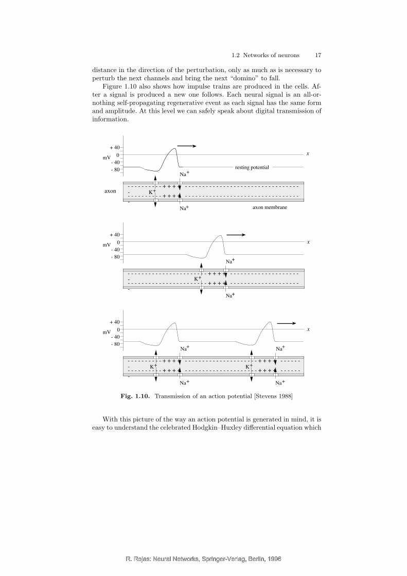
Figure 1.10 shows an action potential traveling through an axon. A localperturbation, produced by the signals arriving at the dendrites, leads to theopening of the sodium-selective channels in a certain region of the cell mem-brane. The membrane is thus depolarized and positive sodium ions flow intothe cell. After a short delay, the outward flow of potassium ions compensatesthe depolarization of the membrane. Both perturbations – the opening of thesodium and potassium-selective channels – are transmitted through the axonlike falling dominos. In the entire process only local energy is consumed, thatis, only the energy stored in the polarized membrane itself. The action po-tential is thus a wave of Na+ permeability increase followed by a wave of K+
permeability increase. It is easy to see that charged particles only move a short
R. Rojas: Neural Networks, Springer-Verlag, Berlin, 1996R. Rojas: Neural Networks, Springer-Verlag, Berlin, 1996
R. Rojas: Neural Networks, Springer-Verlag, Berlin, 1996
1.2 Networks of neurons 17
distance in the direction of the perturbation, only as much as is necessary toperturb the next channels and bring the next “domino” to fall.
Figure 1.10 also shows how impulse trains are produced in the cells. Af-ter a signal is produced a new one follows. Each neural signal is an all-or-nothing self-propagating regenerative event as each signal has the same formand amplitude. At this level we can safely speak about digital transmission ofinformation.
- - - - - - - - - - + + + + - - - - - - - - - - - - - - - - - - - - - - - - - - - - - - - - --- - - - - - - - - - + + + + - - - - - - - - - - - - - - - - - - - - - - - - - - - - - - - - --
+ 40
0
- 40
- 80
mV
Na+
Na+
- - - - - - - - - - - - - - - - - - - - - - - + + + + - - - - - - - - - - - - - - - - - - - --- - - - - - - - - - - - - - - - - - - - - - - + + + + - - - - - - - - - - - - - - - - - - - --
+ 40
0
- 40
- 80
mV
Na+
Na+
- - - - - - - - - - + + + + - - - - - - - - - - - - - - - - - - - - - + + + + - - - - - --- - - - - - - - - - + + + + - - - - - - - - - - - - - - - - - - - - - + + + + - - - - - --
+ 40
0
- 40
- 80
mV
Na+
Na+
Na+
Na+
K+
K+
K+K+
resting potential
axon membrane
axon
x
x
x
Fig. 1.10. Transmission of an action potential [Stevens 1988]
With this picture of the way an action potential is generated in mind, it iseasy to understand the celebrated Hodgkin–Huxley differential equation which
R. Rojas: Neural Networks, Springer-Verlag, Berlin, 1996R. Rojas: Neural Networks, Springer-Verlag, Berlin, 1996
R. Rojas: Neural Networks, Springer-Verlag, Berlin, 1996
18 1 The Biological Paradigm
describes the instantaneous variation of the cell’s potential V as a function ofthe conductances of sodium, potassium and leakages (gNa, gK, gL) and of theequilibrium potentials for all three groups of ions called VNa, VK and VL withrespect to the current potential:
dV
dt=
1
Cm(I − gNa(V − VNa)− gK(V − VK)− gL(V − VL)). (1.1)
In this equation Cm is the capacitance of the cell membrane. The termsV − VNa, V − VK, V − VL are the electromotive forces acting on the ions.Any variation of the conductances translates into a corresponding variationof the cell’s potential V . The variations of gNa and gK are given by differentialequations which describe their oscillations. The conductance of the leakages,gL, can be taken as a constant.
A neuron codes its level of activity by adjusting the frequency of the gen-erated impulses. This frequency is greater for a greater stimulus. In some cellsthe mapping from stimulus to frequency is linear in a certain interval [72].This means that information is transmitted from cell to cell using what engi-neers call frequency modulation. This form of transmission helps to increasethe accuracy of the signal and to minimize the energy consumption of thecells.
1.2.3 Information processing at the neurons and synapses
Neurons transmit information using action potentials. The processing of thisinformation involves a combination of electrical and chemical processes, reg-ulated for the most part at the interface between neurons, the synapses.
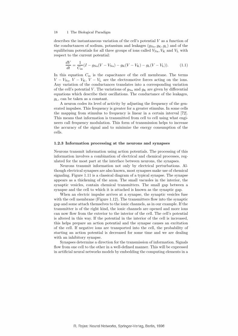
Neurons transmit information not only by electrical perturbations. Al-though electrical synapses are also known, most synapses make use of chemicalsignaling. Figure 1.11 is a classical diagram of a typical synapse. The synapseappears as a thickening of the axon. The small vacuoles in the interior, thesynaptic vesicles, contain chemical transmitters. The small gap between asynapse and the cell to which it is attached is known as the synaptic gap.
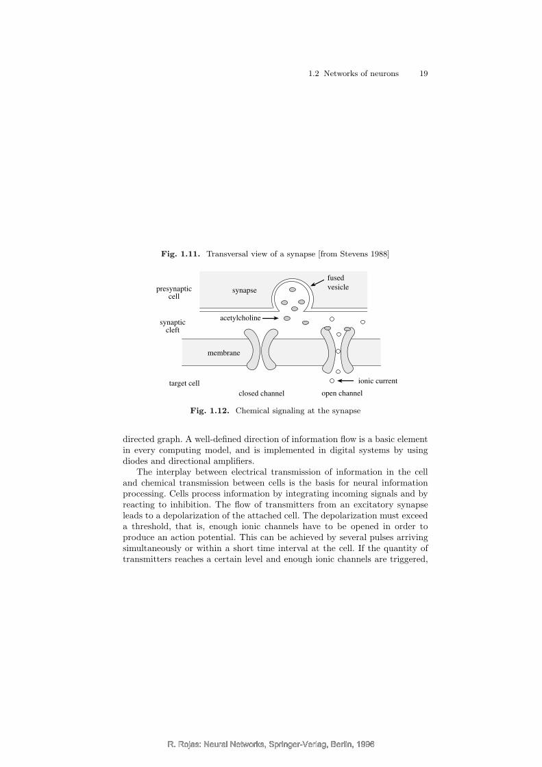
When an electric impulse arrives at a synapse, the synaptic vesicles fusewith the cell membrane (Figure 1.12). The transmitters flow into the synapticgap and some attach themselves to the ionic channels, as in our example. If thetransmitter is of the right kind, the ionic channels are opened and more ionscan now flow from the exterior to the interior of the cell. The cell’s potentialis altered in this way. If the potential in the interior of the cell is increased,this helps prepare an action potential and the synapse causes an excitationof the cell. If negative ions are transported into the cell, the probability ofstarting an action potential is decreased for some time and we are dealingwith an inhibitory synapse.
Synapses determine a direction for the transmission of information. Signalsflow from one cell to the other in a well-defined manner. This will be expressedin artificial neural networks models by embedding the computing elements in a
R. Rojas: Neural Networks, Springer-Verlag, Berlin, 1996R. Rojas: Neural Networks, Springer-Verlag, Berlin, 1996
R. Rojas: Neural Networks, Springer-Verlag, Berlin, 1996
1.2 Networks of neurons 19
Fig. 1.11. Transversal view of a synapse [from Stevens 1988]
membrane
acetylcholine
closed channel open channel
synapse
fused
vesicle
ionic current
synapticcleft
target cell
presynapticcell
Fig. 1.12. Chemical signaling at the synapse
directed graph. A well-defined direction of information flow is a basic elementin every computing model, and is implemented in digital systems by usingdiodes and directional amplifiers.
The interplay between electrical transmission of information in the celland chemical transmission between cells is the basis for neural informationprocessing. Cells process information by integrating incoming signals and byreacting to inhibition. The flow of transmitters from an excitatory synapseleads to a depolarization of the attached cell. The depolarization must exceeda threshold, that is, enough ionic channels have to be opened in order toproduce an action potential. This can be achieved by several pulses arrivingsimultaneously or within a short time interval at the cell. If the quantity oftransmitters reaches a certain level and enough ionic channels are triggered,
R. Rojas: Neural Networks, Springer-Verlag, Berlin, 1996R. Rojas: Neural Networks, Springer-Verlag, Berlin, 1996
R. Rojas: Neural Networks, Springer-Verlag, Berlin, 1996
20 1 The Biological Paradigm
the cell reaches its activation threshold. At this moment an action potentialis generated at the axon of this cell.
In most neurons, action potentials are produced at the so-called axonhillock, the part of the axon nearest to the cell body. In this region of the cell,the number of ionic channels is larger and the cell’s threshold lower [427]. Thedendrites collect the electrical signals which are then transmitted electroton-ically, that is through the cytoplasm [420]. The transmission of informationat the dendrites makes use of additional electrical effects. Streams of ions arecollected at the dendrites and brought to the axon hillock. There is spatialsummation of information when signals coming from different dendrites arecollected, and temporal summation when signals arriving consecutively arecombined to produce a single reaction. In some neurons not only the axonhillock but also the dendrites can produce action potentials. In this case in-formation processing at the cell is more complex than in the standard case.
It can be shown that digital signals combined in an excitatory or inhibitoryway can be used to implement any desired logical function (Chap. 2). Thenumber of computing units required can be reduced if the information is notonly transmitted but also weighted. This can be achieved by multiplying thesignal by a constant. Such is the kind of processing we find at the synapses.Each signal is an all-or-none event but the number of ionic channels triggeredby the signal is different from synapse to synapse. It can happen that a singlesynapse can push a cell to fire an action potential, but other synapses canachieve this only by simultaneously exciting the cell. With each synapse i(1 ≤ i ≤ n) we can therefore associate a numerical weight wi. If all synapsesare activated at the same time, the information which will be transmitted isw1 + w2 + · · ·+ wn. If this value is greater than the cell’s threshold, the cellwill fire a pulse.
It follows from this description that neurons process information at themembrane. The membrane regulates both transmission and processing of in-formation. Summation of signals and comparison with a threshold is a com-bined effect of the membrane and the cytoplasm. If a pulse is generated, itis transmitted and the synapses set some transmitter molecules free. Fromthis description an abstract neuron [72] can be modeled which contains den-drites, a cell body and an axon. The same three elements will be present inour artificial computing units.
1.2.4 Storage of information – learning
In neural networks information is stored at the synapses. Some other forms ofinformation storage may be present, but they are either still unknown or notvery well understood.
A synapse’s efficiency in eliciting the depolarization of the contacted cellcan be increased if more ionic channels are opened. In recent years NMDAreceptors have been studied because they exhibit some properties which couldhelp explain some forms of learning in neurons [72].
R. Rojas: Neural Networks, Springer-Verlag, Berlin, 1996R. Rojas: Neural Networks, Springer-Verlag, Berlin, 1996
R. Rojas: Neural Networks, Springer-Verlag, Berlin, 1996
1.2 Networks of neurons 21
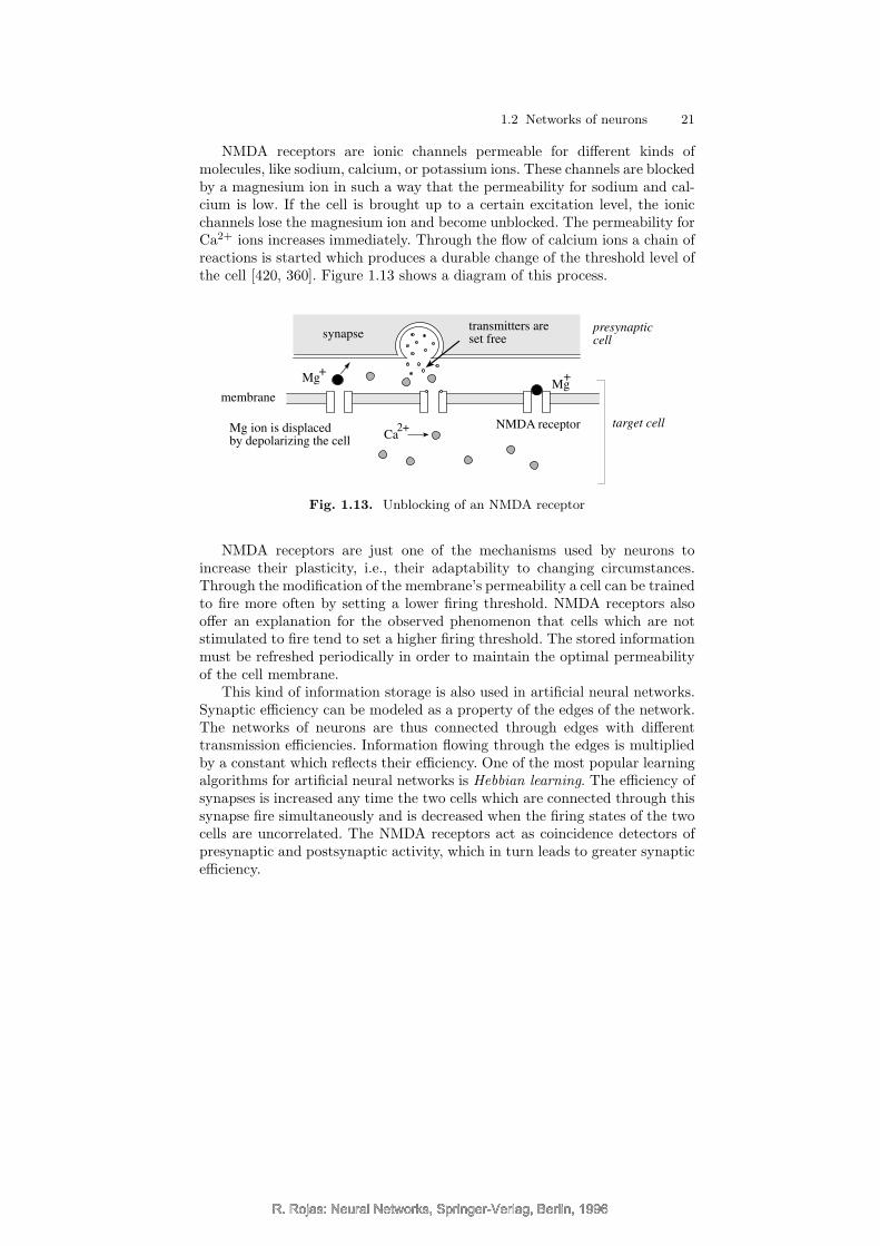
NMDA receptors are ionic channels permeable for different kinds ofmolecules, like sodium, calcium, or potassium ions. These channels are blockedby a magnesium ion in such a way that the permeability for sodium and cal-cium is low. If the cell is brought up to a certain excitation level, the ionicchannels lose the magnesium ion and become unblocked. The permeability forCa2+ ions increases immediately. Through the flow of calcium ions a chain ofreactions is started which produces a durable change of the threshold level ofthe cell [420, 360]. Figure 1.13 shows a diagram of this process.
MgMg
+ +
NMDA receptor
membrane
synapsetransmitters areset free
Mg ion is displacedby depolarizing the cell
presynapticcell
target cellCa
2+
Fig. 1.13. Unblocking of an NMDA receptor
NMDA receptors are just one of the mechanisms used by neurons toincrease their plasticity, i.e., their adaptability to changing circumstances.Through the modification of the membrane’s permeability a cell can be trainedto fire more often by setting a lower firing threshold. NMDA receptors alsooffer an explanation for the observed phenomenon that cells which are notstimulated to fire tend to set a higher firing threshold. The stored informationmust be refreshed periodically in order to maintain the optimal permeabilityof the cell membrane.
This kind of information storage is also used in artificial neural networks.Synaptic efficiency can be modeled as a property of the edges of the network.The networks of neurons are thus connected through edges with differenttransmission efficiencies. Information flowing through the edges is multipliedby a constant which reflects their efficiency. One of the most popular learningalgorithms for artificial neural networks is Hebbian learning. The efficiency ofsynapses is increased any time the two cells which are connected through thissynapse fire simultaneously and is decreased when the firing states of the twocells are uncorrelated. The NMDA receptors act as coincidence detectors ofpresynaptic and postsynaptic activity, which in turn leads to greater synapticefficiency.
R. Rojas: Neural Networks, Springer-Verlag, Berlin, 1996R. Rojas: Neural Networks, Springer-Verlag, Berlin, 1996
R. Rojas: Neural Networks, Springer-Verlag, Berlin, 1996
22 1 The Biological Paradigm
1.2.5 The neuron – a self-organizing system
The short review of the properties of biological neurons in the previous sec-tions is necessarily incomplete and can offer only a rough description of themechanisms and processes by which neurons deal with information. Nerve cellsare very complex self-organizing systems which have evolved in the course ofmillions of years. How were these exquisitely fine-tuned information processingorgans developed? Where do we find the evolutionary origin of consciousness?
The information processing capabilities of neurons depend essentially onthe characteristics of the cell membrane. Ionic channels appeared very early inevolution to allow unicellular organisms to get some kind of feedback from theenvironment. Consider the case of a paramecium, a protozoan with cilia, whichare hairlike processes which provide it with locomotion. A paramecium has amembrane cell with ionic channels and its normal state is one in which theinterior of the cell is negative with respect to the exterior. In this state the ciliaaround the membrane beat rhythmically and propel the paramecium forward.If an obstacle is encountered, some ionic channels sensitive to contact open,let ions into the cell, and depolarize it. The depolarization of the cell leads inturn to a reversing of the beating direction of the cilia and the parameciumswims backward for a short time. After the cytoplasm returns to its normalstate, the paramecium swims forward, changing its direction of movement. Ifthe paramecium is touched from behind, the opening of ionic channels leads toa forward acceleration of the protozoan. In each case, the paramecium escapesits enemies [190].
From these humble origins, ionic channels in neurons have been perfectedover millions of years of evolution. In the protoplasm of the cell, ionic chan-nels are produced and replaced continually. They attach themselves to thoseregions of the neurons where they are needed and can move laterally in themembrane, like icebergs in the sea. The regions of increased neural sensi-tivity to the production of action potentials are thus changing continuouslyaccording to experience. The electrical properties of the cell membrane are nottotally predetermined. They are also a result of the process by which actionpotentials are generated.
Consider also the interior of the neurons. The number of biochemical re-action chains and the complexity of the mechanical processes occurring in theneuron at any given time have led some authors to look for its control system.Stuart Hameroff, for example, has proposed that the cytoskeleton of neuronsdoes not just perform a static mechanical function, but in some way providesthe cell with feedback control. It is well known that the proteins that formthe microtubules in axons coordinate to move synaptic vesicles and other ma-terials from the cell body to the synapses. This is accomplished through acoordinated movement of the proteins, configured like a cellular automaton[173, 174].
Consequently, transmission, storage, and processing of information are per-formed by neurons exploiting many effects and mechanisms which we still do
R. Rojas: Neural Networks, Springer-Verlag, Berlin, 1996R. Rojas: Neural Networks, Springer-Verlag, Berlin, 1996
R. Rojas: Neural Networks, Springer-Verlag, Berlin, 1996
1.3 Artificial neural networks 23
not understand fully. Each individual neuron is as complex or more complexthan any of our computers. For this reason, we will call the elementary compo-nents of artificial neural networks simply “computing units” and not neurons.In the mid-1980s, the PDP (Parallel Distributed Processing) group alreadyagreed to this convention at the insistence of Francis Crick [95].
1.3 Artificial neural networks
The discussion in the last section is only an example of how important it isto define the primitive functions and composition rules of the computationalmodel. If we are computing with a conventional von Neumann processor, aminimal set of machine instructions is needed in order to implement all com-putable functions. In the case of artificial neural networks, the primitive func-tions are located in the nodes of the network and the composition rules arecontained implicitly in the interconnection pattern of the nodes, in the syn-chrony or asynchrony of the transmission of information, and in the presenceor absence of cycles.
1.3.1 Networks of primitive functions
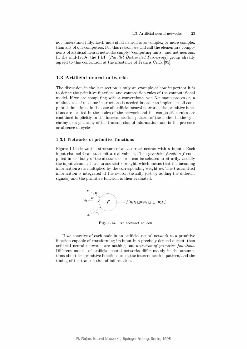
Figure 1.14 shows the structure of an abstract neuron with n inputs. Eachinput channel i can transmit a real value xi. The primitive function f com-puted in the body of the abstract neuron can be selected arbitrarily. Usuallythe input channels have an associated weight, which means that the incominginformation xi is multiplied by the corresponding weight wi. The transmittedinformation is integrated at the neuron (usually just by adding the differentsignals) and the primitive function is then evaluated.
f (w1 x1 + w2 x2 + + wnxn )
w1
w2
wn
x1
x2
xn
f...
...
Fig. 1.14. An abstract neuron
If we conceive of each node in an artificial neural network as a primitivefunction capable of transforming its input in a precisely defined output, thenartificial neural networks are nothing but networks of primitive functions.Different models of artificial neural networks differ mainly in the assump-tions about the primitive functions used, the interconnection pattern, and thetiming of the transmission of information.
R. Rojas: Neural Networks, Springer-Verlag, Berlin, 1996R. Rojas: Neural Networks, Springer-Verlag, Berlin, 1996
R. Rojas: Neural Networks, Springer-Verlag, Berlin, 1996
24 1 The Biological Paradigm
x
y
z
f
f
f
f1
2
3
4 (x, y, z)
α
α
α
α
α
1
2
3
4
5
Φ
Fig. 1.15. Functional model of an artificial neural network
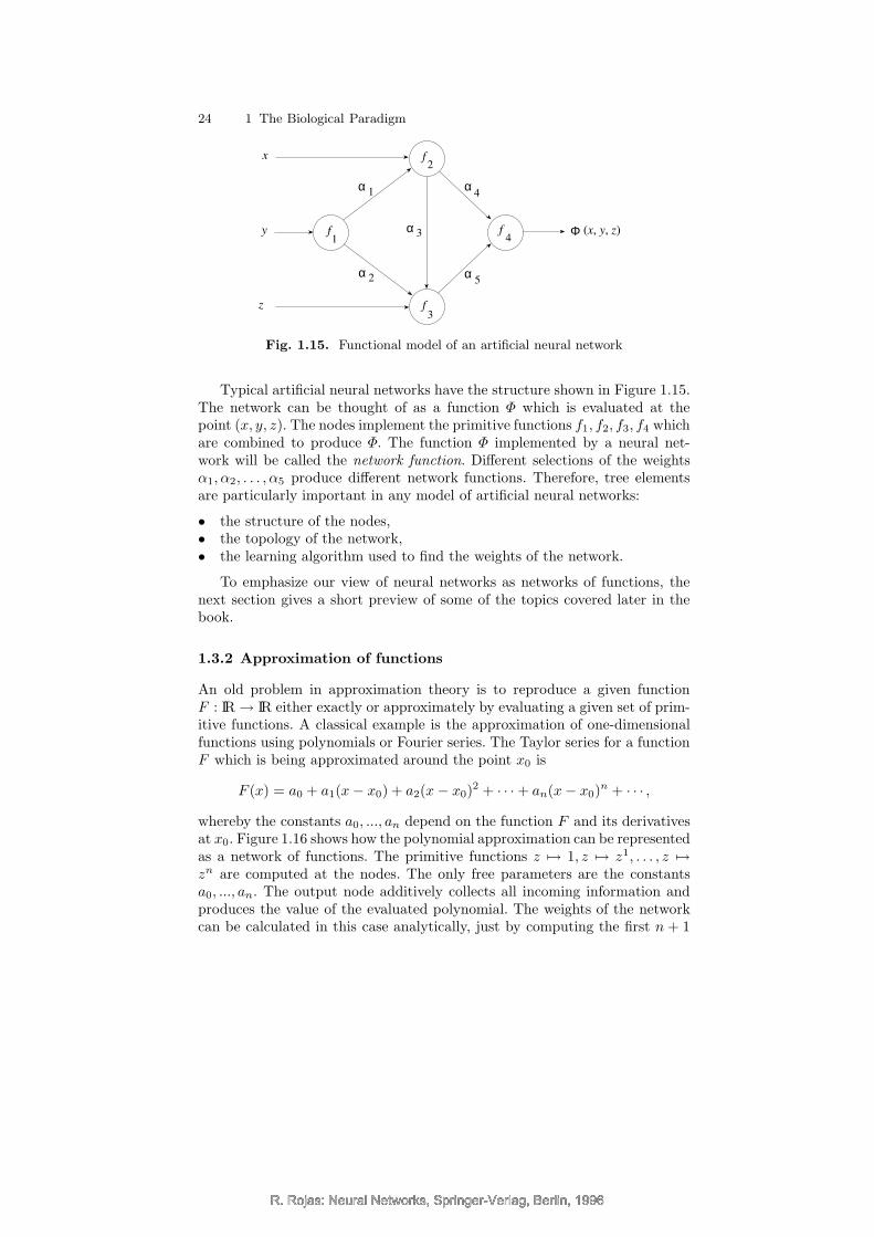
Typical artificial neural networks have the structure shown in Figure 1.15.The network can be thought of as a function Φ which is evaluated at thepoint (x, y, z). The nodes implement the primitive functions f1, f2, f3, f4 whichare combined to produce Φ. The function Φ implemented by a neural net-work will be called the network function. Different selections of the weightsα1, α2, . . . , α5 produce different network functions. Therefore, tree elementsare particularly important in any model of artificial neural networks:
• the structure of the nodes,• the topology of the network,• the learning algorithm used to find the weights of the network.
To emphasize our view of neural networks as networks of functions, thenext section gives a short preview of some of the topics covered later in thebook.
1.3.2 Approximation of functions
An old problem in approximation theory is to reproduce a given functionF : IR→ IR either exactly or approximately by evaluating a given set of prim-itive functions. A classical example is the approximation of one-dimensionalfunctions using polynomials or Fourier series. The Taylor series for a functionF which is being approximated around the point x0 is
F (x) = a0 + a1(x− x0) + a2(x − x0)2 + · · ·+ an(x− x0)
n + · · · ,
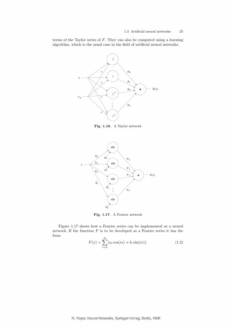
whereby the constants a0, ..., an depend on the function F and its derivativesat x0. Figure 1.16 shows how the polynomial approximation can be representedas a network of functions. The primitive functions z 7→ 1, z 7→ z1, . . . , z 7→zn are computed at the nodes. The only free parameters are the constantsa0, ..., an. The output node additively collects all incoming information andproduces the value of the evaluated polynomial. The weights of the networkcan be calculated in this case analytically, just by computing the first n + 1
R. Rojas: Neural Networks, Springer-Verlag, Berlin, 1996R. Rojas: Neural Networks, Springer-Verlag, Berlin, 1996
R. Rojas: Neural Networks, Springer-Verlag, Berlin, 1996
1.3 Artificial neural networks 25
terms of the Taylor series of F . They can also be computed using a learningalgorithm, which is the usual case in the field of artificial neural networks.
+
z
z
x
F(x)
1
2
z n
a0
a1
an
a2
x0
-1
-1
-1
-1
...
Fig. 1.16. A Taylor network
+
x
F(x)
w0
w1
wn
w2
sin
sin
sin
sin
k0
k1
kn
k 2
d0
d1
d2 ...
dn
Fig. 1.17. A Fourier network
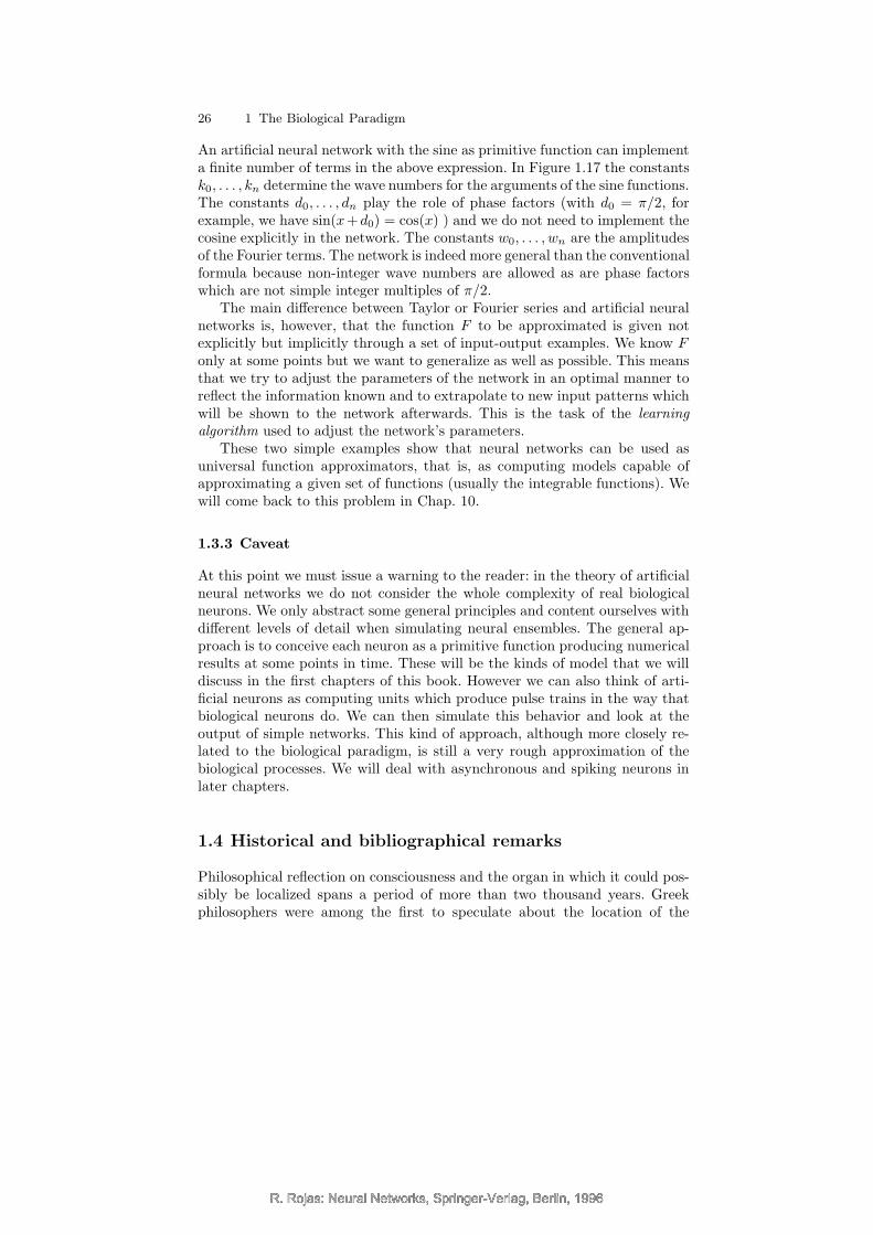
Figure 1.17 shows how a Fourier series can be implemented as a neuralnetwork. If the function F is to be developed as a Fourier series it has theform
F (x) =∞∑
i=0
(ai cos(ix) + bi sin(ix)). (1.2)
R. Rojas: Neural Networks, Springer-Verlag, Berlin, 1996R. Rojas: Neural Networks, Springer-Verlag, Berlin, 1996
R. Rojas: Neural Networks, Springer-Verlag, Berlin, 1996
26 1 The Biological Paradigm
An artificial neural network with the sine as primitive function can implementa finite number of terms in the above expression. In Figure 1.17 the constantsk0, . . . , kn determine the wave numbers for the arguments of the sine functions.The constants d0, . . . , dn play the role of phase factors (with d0 = π/2, forexample, we have sin(x+d0) = cos(x) ) and we do not need to implement thecosine explicitly in the network. The constants w0, . . . , wn are the amplitudesof the Fourier terms. The network is indeed more general than the conventionalformula because non-integer wave numbers are allowed as are phase factorswhich are not simple integer multiples of π/2.
The main difference between Taylor or Fourier series and artificial neuralnetworks is, however, that the function F to be approximated is given notexplicitly but implicitly through a set of input-output examples. We know Fonly at some points but we want to generalize as well as possible. This meansthat we try to adjust the parameters of the network in an optimal manner toreflect the information known and to extrapolate to new input patterns whichwill be shown to the network afterwards. This is the task of the learningalgorithm used to adjust the network’s parameters.
These two simple examples show that neural networks can be used asuniversal function approximators, that is, as computing models capable ofapproximating a given set of functions (usually the integrable functions). Wewill come back to this problem in Chap. 10.
1.3.3 Caveat
At this point we must issue a warning to the reader: in the theory of artificialneural networks we do not consider the whole complexity of real biologicalneurons. We only abstract some general principles and content ourselves withdifferent levels of detail when simulating neural ensembles. The general ap-proach is to conceive each neuron as a primitive function producing numericalresults at some points in time. These will be the kinds of model that we willdiscuss in the first chapters of this book. However we can also think of arti-ficial neurons as computing units which produce pulse trains in the way thatbiological neurons do. We can then simulate this behavior and look at theoutput of simple networks. This kind of approach, although more closely re-lated to the biological paradigm, is still a very rough approximation of thebiological processes. We will deal with asynchronous and spiking neurons inlater chapters.
1.4 Historical and bibliographical remarks
Philosophical reflection on consciousness and the organ in which it could pos-sibly be localized spans a period of more than two thousand years. Greekphilosophers were among the first to speculate about the location of the
R. Rojas: Neural Networks, Springer-Verlag, Berlin, 1996R. Rojas: Neural Networks, Springer-Verlag, Berlin, 1996
R. Rojas: Neural Networks, Springer-Verlag, Berlin, 1996
1.4 Historical and bibliographical remarks 27
soul. Several theories were held by the various philosophical schools of an-cient times. Galenus, for example, identified nerve impulses with pneumaticpressure signals and conceived the nervous system as a pneumatic machine.Several centuries later Newton speculated that nerves transmitted oscillationsof the ether.
Our present knowledge of the structure and physiology of neurons is theresult of 100 years of special research in this field. The facts presented in thischapter were discovered between 1850 and 1950, with the exception of theNMDA receptors which were studied mainly in the last decade. The electri-cal nature of nerve impulses was postulated around 1850 by Emil du Bois-Reymond and Hermann von Helmholtz. The latter was able to measure thevelocity of nerve impulses and showed that it was not as fast as was previ-ously thought. Signals can be transmitted in both directions of an axon, butaround 1901 Santiago Ramon y Cajal postulated that the specific networkingof the nervous cells determines a direction for the transmission of information.This discovery made it clear that the coupling of the neurons constitutes ahierarchical system.
Ramon y Cajal was also the most celebrated advocate of the neuron the-ory. His supporters conceived the brain as a highly differentiated hierarchicalorgan, while the supporters of the reticular theory thought of the brain as agrid of undifferentiated axons and of dendrites as organs for the nutrition ofthe cell [357]. Ramon y Cajal perfected Golgi’s staining method and publishedthe best diagrams of neurons of his time, so good indeed that they are still inuse. The word neuron (Greek for nerve) was proposed by the Berlin ProfessorWilhelm Waldeger after he saw the preparations of Ramon y Cajal [418].
The chemical transmission of information at the synapses was studied from1920 to 1940. From 1949 to 1956, Hodgkin and Huxley explained the mech-anism by which depolarization waves are produced in the cell membrane. Byexperimenting with the giant axon of the squid they measured and explainedthe exchange of ions through the cell membrane, which in time led to the nowfamous Hodgkin–Huxley differential equations. For a mathematical treatmentof this system of equations see [97].
The Hodgkin–Huxley model was in some ways one of the first artificial neu-ral models, because the postulated dynamics of the nerve impulses could besimulated with simple electric networks [303]. At the same time the mathemat-ical properties of artificial neural networks were being studied by researcherslike Warren McCulloch, Walter Pitts, and John von Neumann. Ever since thattime, research in the neurobiological field has progressed in close collaborationwith the mathematics and computer science community.
Exercises
1. Express the network function function Φ in Figure 1.15 in terms of theprimitive functions f1, . . . , f4 and of the weights α1, . . . , α5.
R. Rojas: Neural Networks, Springer-Verlag, Berlin, 1996R. Rojas: Neural Networks, Springer-Verlag, Berlin, 1996

R. Rojas: Neural Networks, Springer-Verlag, Berlin, 1996
28 1 The Biological Paradigm
2. Modify the network of Figure 1.17 so that it corresponds to a finite numberof addition terms of equation (1.2).
3. Look in a neurobiology book for the full set of differential equations ofthe Hodgkin–Huxley model. Write a computer program that simulates anaction potential.
R. Rojas: Neural Networks, Springer-Verlag, Berlin, 1996R. Rojas: Neural Networks, Springer-Verlag, Berlin, 1996
R. Rojas: Neural Networks, Springer-Verlag, Berlin, 1996
2
Threshold Logic
2.1 Networks of functions
We deal in this chapter with the simplest kind of computing units used tobuild artificial neural networks. These computing elements are a generalizationof the common logic gates used in conventional computing and, since theyoperate by comparing their total input with a threshold, this field of researchis known as threshold logic.
2.1.1 Feed-forward and recurrent networks
Our review in the previous chapter of the characteristics and structure of bi-ological neural networks provides us with the initial motivation for a deeperinquiry into the properties of networks of abstract neurons. From the view-point of the engineer, it is important to define how a network should behave,without having to specify completely all of its parameters, which are to befound in a learning process. Artificial neural networks are used in many casesas a black box : a certain input should produce a desired output, but how thenetwork achieves this result is left to a self-organizing process.
x1
x2
xn
y1
y2
ym
F...
...
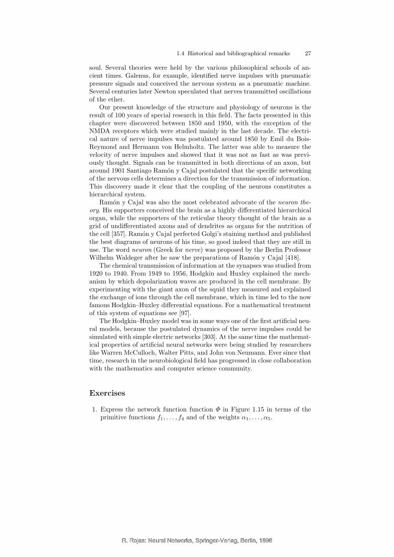
Fig. 2.1. A neural network as a black box
In general we are interested in mapping an n-dimensional real input(x1, x2, . . . , xn) to an m-dimensional real output (y1, y2, . . . , ym). A neural
R. Rojas: Neural Networks, Springer-Verlag, Berlin, 1996R. Rojas: Neural Networks, Springer-Verlag, Berlin, 1996
R. Rojas: Neural Networks, Springer-Verlag, Berlin, 1996
30 2 Threshold Logic
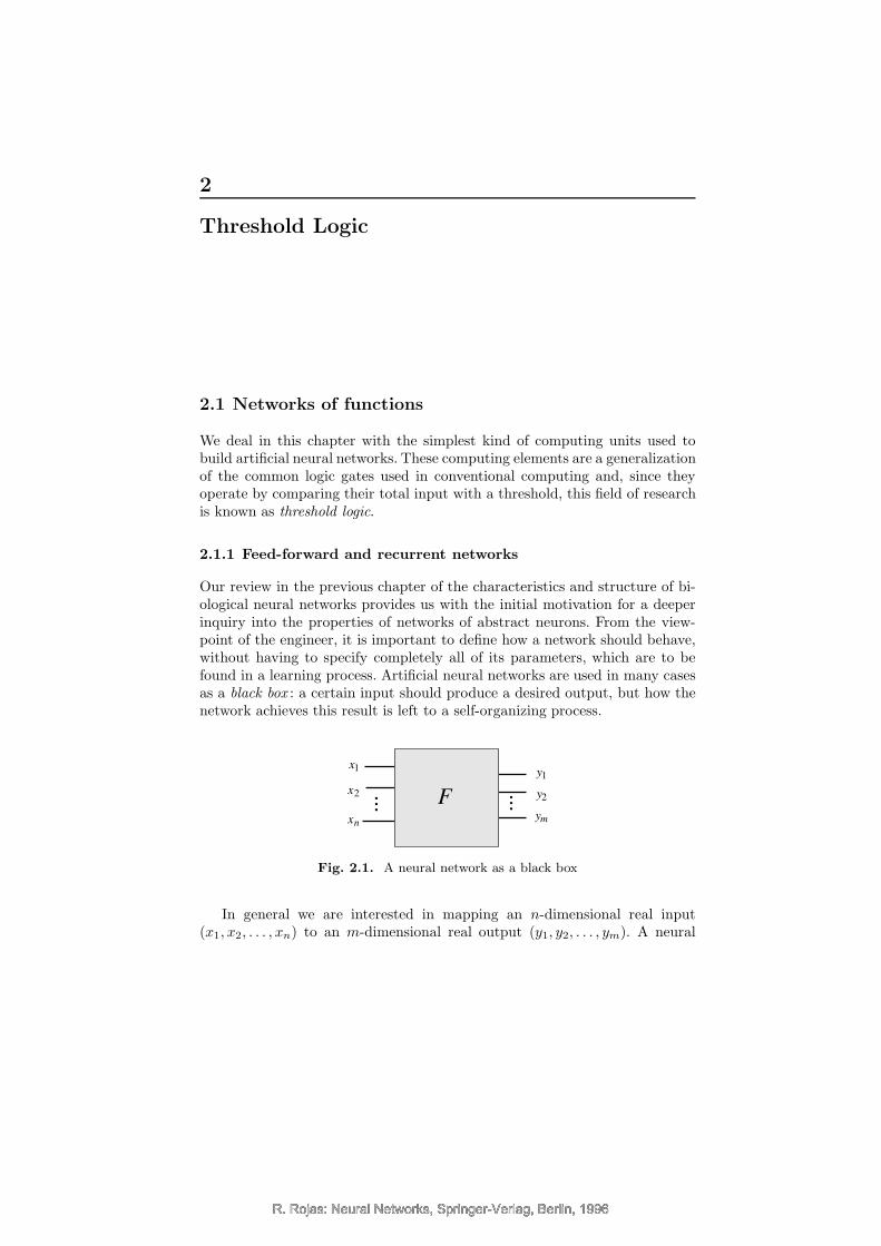
network thus behaves as a “mapping machine”, capable of modeling a func-tion F : IRn → IRm. If we look at the structure of the network being used, someaspects of its dynamics must be defined more precisely. When the functionis evaluated with a network of primitive functions, information flows throughthe directed edges of the network. Some nodes compute values which are thentransmitted as arguments for new computations. If there are no cycles in thenetwork, the result of the whole computation is well-defined and we do nothave to deal with the task of synchronizing the computing units. We justassume that the computations take place without delay.
f
gx g(x)
f (g (x))
Fig. 2.2. Function composition
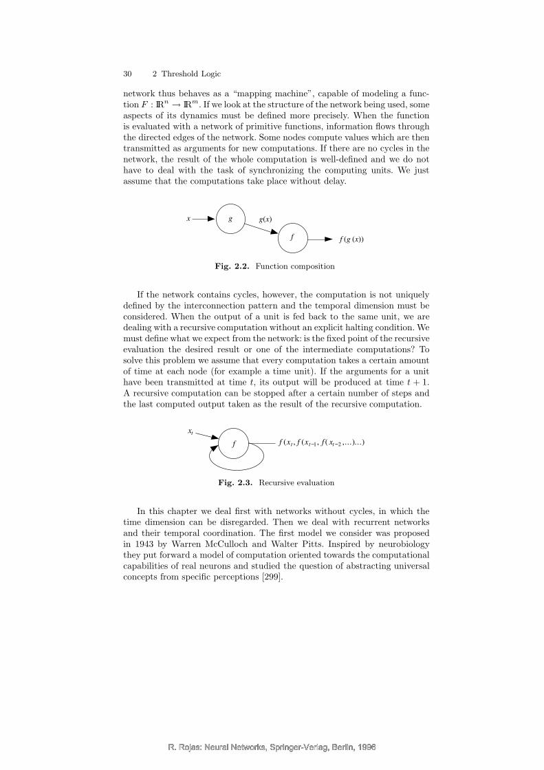
If the network contains cycles, however, the computation is not uniquelydefined by the interconnection pattern and the temporal dimension must beconsidered. When the output of a unit is fed back to the same unit, we aredealing with a recursive computation without an explicit halting condition. Wemust define what we expect from the network: is the fixed point of the recursiveevaluation the desired result or one of the intermediate computations? Tosolve this problem we assume that every computation takes a certain amountof time at each node (for example a time unit). If the arguments for a unithave been transmitted at time t, its output will be produced at time t + 1.A recursive computation can be stopped after a certain number of steps andthe last computed output taken as the result of the recursive computation.
f f (xt , f (xt−1, f ( xt −2 ,...)...)
xt
Fig. 2.3. Recursive evaluation
In this chapter we deal first with networks without cycles, in which thetime dimension can be disregarded. Then we deal with recurrent networksand their temporal coordination. The first model we consider was proposedin 1943 by Warren McCulloch and Walter Pitts. Inspired by neurobiologythey put forward a model of computation oriented towards the computationalcapabilities of real neurons and studied the question of abstracting universalconcepts from specific perceptions [299].
R. Rojas: Neural Networks, Springer-Verlag, Berlin, 1996R. Rojas: Neural Networks, Springer-Verlag, Berlin, 1996
R. Rojas: Neural Networks, Springer-Verlag, Berlin, 1996
2.1 Networks of functions 31
We will avoid giving a general definition of a neural network at this point.So many models have been proposed which differ in so many respects that anydefinition trying to encompass this variety would be unnecessarily clumsy. Aswe show in this chapter, it is not necessary to start building neural networkswith “high powered” computing units, as some authors do [384]. We will startour investigations with the general notion that a neural network is a networkof functions in which synchronization can be considered explicitly or not.
2.1.2 The computing units
The nodes of the networks we consider will be called computing elements orsimply units. We assume that the edges of the network transmit informationin a predetermined direction and the number of incoming edges into a nodeis not restricted by some upper bound. This is called the unlimited fan-inproperty of our computing units.
x1
x2
xn
f f (x1 , x2 , ..., xn )
Fig. 2.4. Evaluation of a function of n arguments
The primitive function computed at each node is in general a function of narguments. Normally, however, we try to use very simple primitive functionsof one argument at the nodes. This means that the incoming n argumentshave to be reduced to a single numerical value. Therefore computing unitsare split into two functional parts: an integration function g reduces the narguments to a single value and the output or activation function f producesthe output of this node taking that single value as its argument. Figure 2.5shows this general structure of the computing units. Usually the integrationfunction g is the addition function.
fg
x1
x2
xn
f (g(x1 , x2 ,..., xn ))
Fig. 2.5. Generic computing unit
McCulloch–Pitts networks are even simpler than this, because they usesolely binary signals, i.e., ones or zeros. The nodes produce only binary results
R. Rojas: Neural Networks, Springer-Verlag, Berlin, 1996R. Rojas: Neural Networks, Springer-Verlag, Berlin, 1996
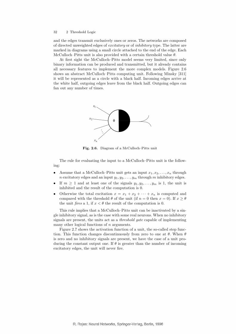
R. Rojas: Neural Networks, Springer-Verlag, Berlin, 1996
32 2 Threshold Logic
and the edges transmit exclusively ones or zeros. The networks are composedof directed unweighted edges of excitatory or of inhibitory type. The latter aremarked in diagrams using a small circle attached to the end of the edge. EachMcCulloch–Pitts unit is also provided with a certain threshold value θ.
At first sight the McCulloch–Pitts model seems very limited, since onlybinary information can be produced and transmitted, but it already containsall necessary features to implement the more complex models. Figure 2.6shows an abstract McCulloch–Pitts computing unit. Following Minsky [311]it will be represented as a circle with a black half. Incoming edges arrive atthe white half, outgoing edges leave from the black half. Outgoing edges canfan out any number of times.
x1
xn
x2 θ
...
Fig. 2.6. Diagram of a McCulloch–Pitts unit
The rule for evaluating the input to a McCulloch–Pitts unit is the follow-ing:
• Assume that a McCulloch–Pitts unit gets an input x1, x2, . . . , xn throughn excitatory edges and an input y1, y2, . . . , ym throughm inhibitory edges.
• If m ≥ 1 and at least one of the signals y1, y2, . . . , ym is 1, the unit isinhibited and the result of the computation is 0.
• Otherwise the total excitation x = x1 + x2 + · · · + xn is computed andcompared with the threshold θ of the unit (if n = 0 then x = 0). If x ≥ θthe unit fires a 1, if x < θ the result of the computation is 0.
This rule implies that a McCulloch–Pitts unit can be inactivated by a sin-gle inhibitory signal, as is the case with some real neurons. When no inhibitorysignals are present, the units act as a threshold gate capable of implementingmany other logical functions of n arguments.
Figure 2.7 shows the activation function of a unit, the so-called step func-tion. This function changes discontinuously from zero to one at θ. When θis zero and no inhibitory signals are present, we have the case of a unit pro-ducing the constant output one. If θ is greater than the number of incomingexcitatory edges, the unit will never fire.
R. Rojas: Neural Networks, Springer-Verlag, Berlin, 1996R. Rojas: Neural Networks, Springer-Verlag, Berlin, 1996
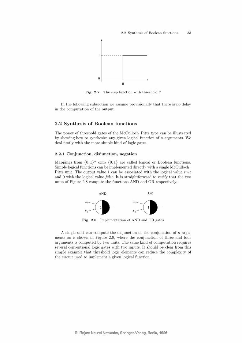
R. Rojas: Neural Networks, Springer-Verlag, Berlin, 1996
2.2 Synthesis of Boolean functions 33
θ
1
0
Fig. 2.7. The step function with threshold θ
In the following subsection we assume provisionally that there is no delayin the computation of the output.
2.2 Synthesis of Boolean functions
The power of threshold gates of the McCulloch–Pitts type can be illustratedby showing how to synthesize any given logical function of n arguments. Wedeal firstly with the more simple kind of logic gates.
2.2.1 Conjunction, disjunction, negation
Mappings from {0, 1}n onto {0, 1} are called logical or Boolean functions.Simple logical functions can be implemented directly with a single McCulloch–Pitts unit. The output value 1 can be associated with the logical value trueand 0 with the logical value false. It is straightforward to verify that the twounits of Figure 2.8 compute the functions AND and OR respectively.
2 1
AND OR
x1
x2 x2
x1
Fig. 2.8. Implementation of AND and OR gates
A single unit can compute the disjunction or the conjunction of n argu-ments as is shown in Figure 2.9, where the conjunction of three and fourarguments is computed by two units. The same kind of computation requiresseveral conventional logic gates with two inputs. It should be clear from thissimple example that threshold logic elements can reduce the complexity ofthe circuit used to implement a given logical function.
R. Rojas: Neural Networks, Springer-Verlag, Berlin, 1996R. Rojas: Neural Networks, Springer-Verlag, Berlin, 1996
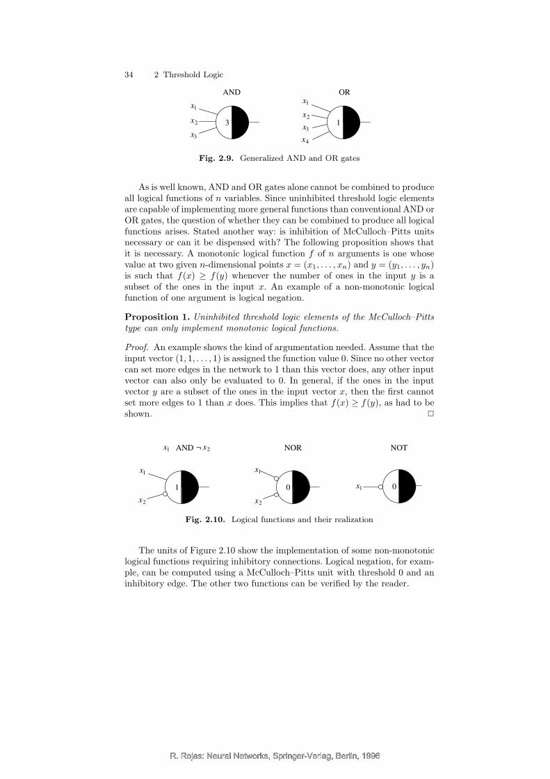
R. Rojas: Neural Networks, Springer-Verlag, Berlin, 1996
34 2 Threshold Logic
3 1
AND OR
x1
x1
x2
x2
x3
x3
x4
Fig. 2.9. Generalized AND and OR gates
As is well known, AND and OR gates alone cannot be combined to produceall logical functions of n variables. Since uninhibited threshold logic elementsare capable of implementing more general functions than conventional AND orOR gates, the question of whether they can be combined to produce all logicalfunctions arises. Stated another way: is inhibition of McCulloch–Pitts unitsnecessary or can it be dispensed with? The following proposition shows thatit is necessary. A monotonic logical function f of n arguments is one whosevalue at two given n-dimensional points x = (x1, . . . , xn) and y = (y1, . . . , yn)is such that f(x) ≥ f(y) whenever the number of ones in the input y is asubset of the ones in the input x. An example of a non-monotonic logicalfunction of one argument is logical negation.
Proposition 1. Uninhibited threshold logic elements of the McCulloch–Pittstype can only implement monotonic logical functions.
Proof. An example shows the kind of argumentation needed. Assume that theinput vector (1, 1, . . . , 1) is assigned the function value 0. Since no other vectorcan set more edges in the network to 1 than this vector does, any other inputvector can also only be evaluated to 0. In general, if the ones in the inputvector y are a subset of the ones in the input vector x, then the first cannotset more edges to 1 than x does. This implies that f(x) ≥ f(y), as had to beshown. 2
1 0
AND NOR¬
0
NOT
x1 x1
x1
x2 x2
x1 x2
Fig. 2.10. Logical functions and their realization
The units of Figure 2.10 show the implementation of some non-monotoniclogical functions requiring inhibitory connections. Logical negation, for exam-ple, can be computed using a McCulloch–Pitts unit with threshold 0 and aninhibitory edge. The other two functions can be verified by the reader.
R. Rojas: Neural Networks, Springer-Verlag, Berlin, 1996R. Rojas: Neural Networks, Springer-Verlag, Berlin, 1996
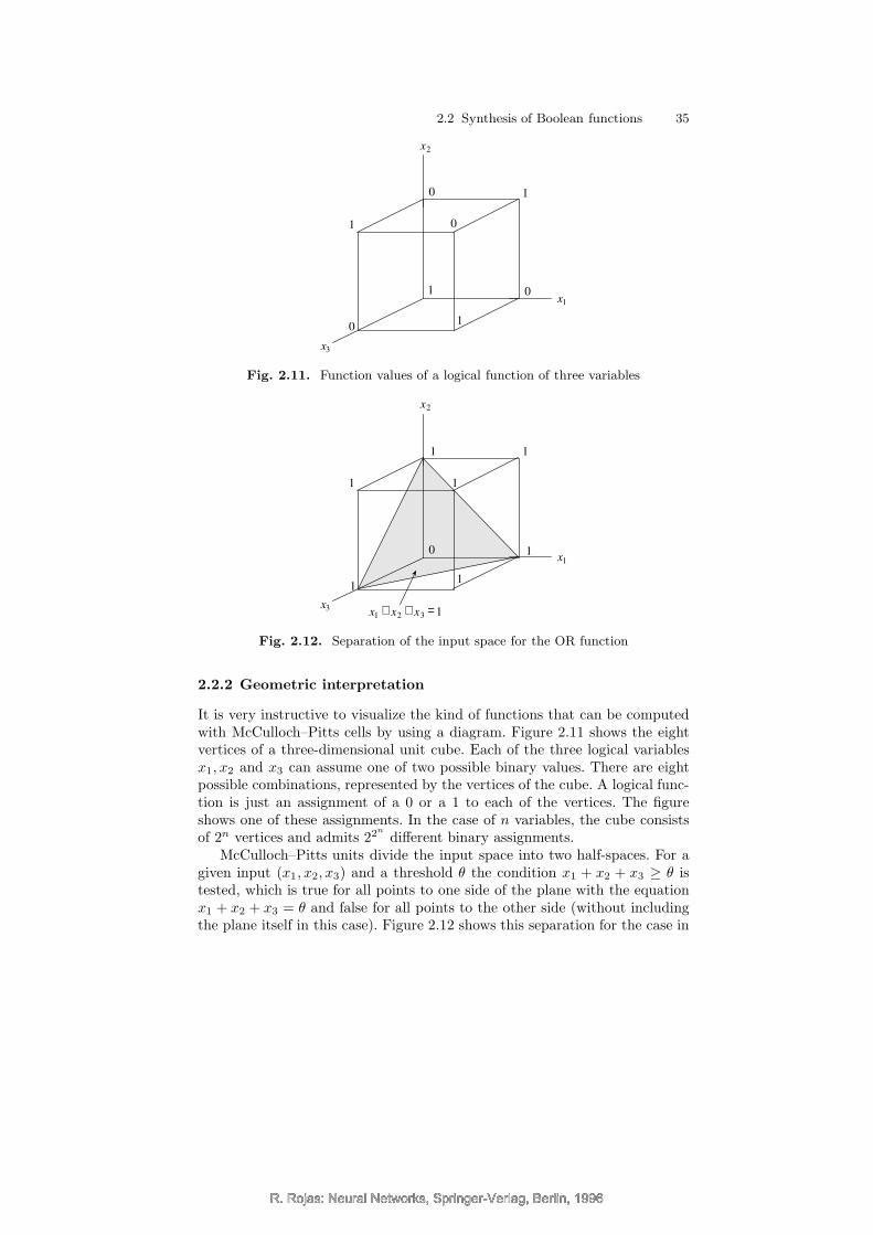
R. Rojas: Neural Networks, Springer-Verlag, Berlin, 1996
2.2 Synthesis of Boolean functions 35
1
1
1
0
0
0
0
1x1
x2
x3
Fig. 2.11. Function values of a logical function of three variables
1
1
1
1
1
1
1
0x1
x2
x3 x1 + x2 + x3 = 1
Fig. 2.12. Separation of the input space for the OR function
2.2.2 Geometric interpretation
It is very instructive to visualize the kind of functions that can be computedwith McCulloch–Pitts cells by using a diagram. Figure 2.11 shows the eightvertices of a three-dimensional unit cube. Each of the three logical variablesx1, x2 and x3 can assume one of two possible binary values. There are eightpossible combinations, represented by the vertices of the cube. A logical func-tion is just an assignment of a 0 or a 1 to each of the vertices. The figureshows one of these assignments. In the case of n variables, the cube consistsof 2n vertices and admits 22n
different binary assignments.McCulloch–Pitts units divide the input space into two half-spaces. For a
given input (x1, x2, x3) and a threshold θ the condition x1 + x2 + x3 ≥ θ istested, which is true for all points to one side of the plane with the equationx1 + x2 + x3 = θ and false for all points to the other side (without includingthe plane itself in this case). Figure 2.12 shows this separation for the case in
R. Rojas: Neural Networks, Springer-Verlag, Berlin, 1996R. Rojas: Neural Networks, Springer-Verlag, Berlin, 1996
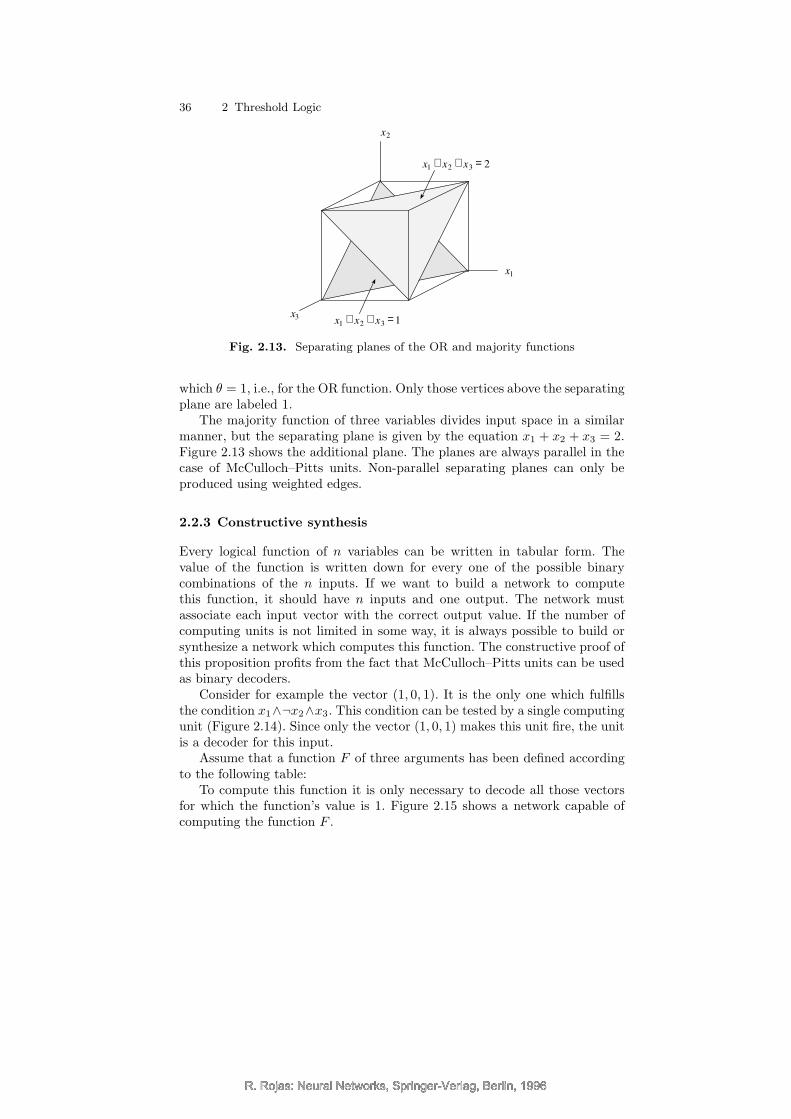
R. Rojas: Neural Networks, Springer-Verlag, Berlin, 1996
36 2 Threshold Logic
x1
x2
x3 x1 + x2 + x3 = 1
x1 + x2 + x3 = 2
Fig. 2.13. Separating planes of the OR and majority functions
which θ = 1, i.e., for the OR function. Only those vertices above the separatingplane are labeled 1.
The majority function of three variables divides input space in a similarmanner, but the separating plane is given by the equation x1 + x2 + x3 = 2.Figure 2.13 shows the additional plane. The planes are always parallel in thecase of McCulloch–Pitts units. Non-parallel separating planes can only beproduced using weighted edges.
2.2.3 Constructive synthesis
Every logical function of n variables can be written in tabular form. Thevalue of the function is written down for every one of the possible binarycombinations of the n inputs. If we want to build a network to computethis function, it should have n inputs and one output. The network mustassociate each input vector with the correct output value. If the number ofcomputing units is not limited in some way, it is always possible to build orsynthesize a network which computes this function. The constructive proof ofthis proposition profits from the fact that McCulloch–Pitts units can be usedas binary decoders.
Consider for example the vector (1, 0, 1). It is the only one which fulfillsthe condition x1∧¬x2∧x3. This condition can be tested by a single computingunit (Figure 2.14). Since only the vector (1, 0, 1) makes this unit fire, the unitis a decoder for this input.
Assume that a function F of three arguments has been defined accordingto the following table:
To compute this function it is only necessary to decode all those vectorsfor which the function’s value is 1. Figure 2.15 shows a network capable ofcomputing the function F .
R. Rojas: Neural Networks, Springer-Verlag, Berlin, 1996R. Rojas: Neural Networks, Springer-Verlag, Berlin, 1996
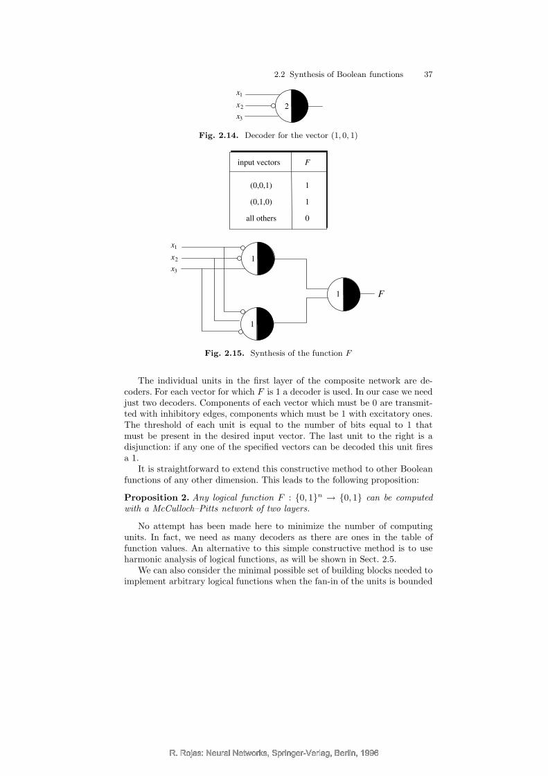
R. Rojas: Neural Networks, Springer-Verlag, Berlin, 1996
2.2 Synthesis of Boolean functions 37
2
x1
x2
x3
Fig. 2.14. Decoder for the vector (1, 0, 1)
input vectors F
(0,0,1) 1
(0,1,0) 1
all others 0
1
1
1
x1
x2
x3
F
Fig. 2.15. Synthesis of the function F
The individual units in the first layer of the composite network are de-coders. For each vector for which F is 1 a decoder is used. In our case we needjust two decoders. Components of each vector which must be 0 are transmit-ted with inhibitory edges, components which must be 1 with excitatory ones.The threshold of each unit is equal to the number of bits equal to 1 thatmust be present in the desired input vector. The last unit to the right is adisjunction: if any one of the specified vectors can be decoded this unit firesa 1.
It is straightforward to extend this constructive method to other Booleanfunctions of any other dimension. This leads to the following proposition:
Proposition 2. Any logical function F : {0, 1}n → {0, 1} can be computedwith a McCulloch–Pitts network of two layers.
No attempt has been made here to minimize the number of computingunits. In fact, we need as many decoders as there are ones in the table offunction values. An alternative to this simple constructive method is to useharmonic analysis of logical functions, as will be shown in Sect. 2.5.
We can also consider the minimal possible set of building blocks needed toimplement arbitrary logical functions when the fan-in of the units is bounded
R. Rojas: Neural Networks, Springer-Verlag, Berlin, 1996R. Rojas: Neural Networks, Springer-Verlag, Berlin, 1996
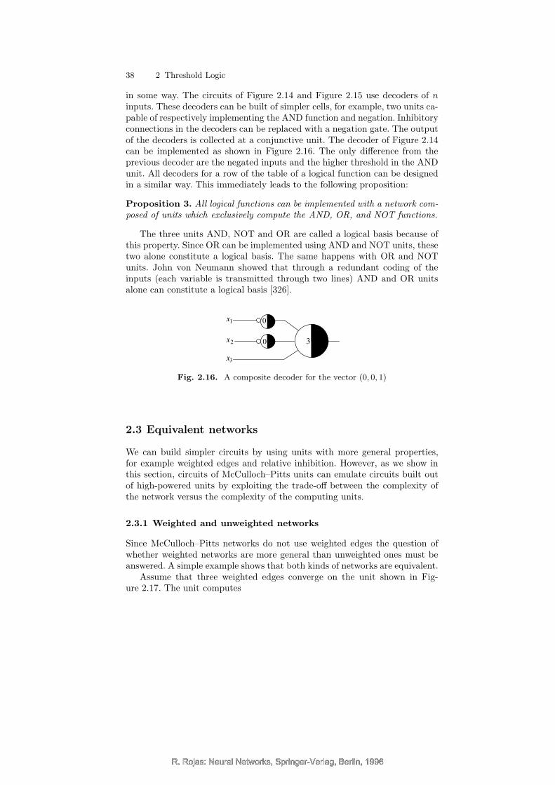
R. Rojas: Neural Networks, Springer-Verlag, Berlin, 1996
38 2 Threshold Logic
in some way. The circuits of Figure 2.14 and Figure 2.15 use decoders of ninputs. These decoders can be built of simpler cells, for example, two units ca-pable of respectively implementing the AND function and negation. Inhibitoryconnections in the decoders can be replaced with a negation gate. The outputof the decoders is collected at a conjunctive unit. The decoder of Figure 2.14can be implemented as shown in Figure 2.16. The only difference from theprevious decoder are the negated inputs and the higher threshold in the ANDunit. All decoders for a row of the table of a logical function can be designedin a similar way. This immediately leads to the following proposition:
Proposition 3. All logical functions can be implemented with a network com-posed of units which exclusively compute the AND, OR, and NOT functions.
The three units AND, NOT and OR are called a logical basis because ofthis property. Since OR can be implemented using AND and NOT units, thesetwo alone constitute a logical basis. The same happens with OR and NOTunits. John von Neumann showed that through a redundant coding of theinputs (each variable is transmitted through two lines) AND and OR unitsalone can constitute a logical basis [326].
3
x1
x2
x3
0
0
Fig. 2.16. A composite decoder for the vector (0, 0, 1)
2.3 Equivalent networks
We can build simpler circuits by using units with more general properties,for example weighted edges and relative inhibition. However, as we show inthis section, circuits of McCulloch–Pitts units can emulate circuits built outof high-powered units by exploiting the trade-off between the complexity ofthe network versus the complexity of the computing units.
2.3.1 Weighted and unweighted networks
Since McCulloch–Pitts networks do not use weighted edges the question ofwhether weighted networks are more general than unweighted ones must beanswered. A simple example shows that both kinds of networks are equivalent.
Assume that three weighted edges converge on the unit shown in Fig-ure 2.17. The unit computes
R. Rojas: Neural Networks, Springer-Verlag, Berlin, 1996R. Rojas: Neural Networks, Springer-Verlag, Berlin, 1996
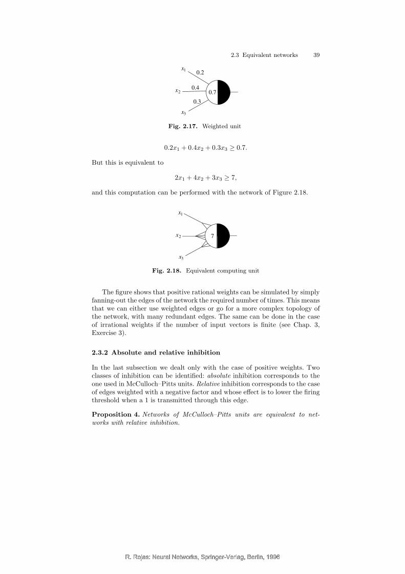
R. Rojas: Neural Networks, Springer-Verlag, Berlin, 1996
2.3 Equivalent networks 39
0.7
0.2
0.4
0.3
x1
x2
x3
Fig. 2.17. Weighted unit
0.2x1 + 0.4x2 + 0.3x3 ≥ 0.7.
But this is equivalent to
2x1 + 4x2 + 3x3 ≥ 7,
and this computation can be performed with the network of Figure 2.18.
x1
x2
x3
7
Fig. 2.18. Equivalent computing unit
The figure shows that positive rational weights can be simulated by simplyfanning-out the edges of the network the required number of times. This meansthat we can either use weighted edges or go for a more complex topology ofthe network, with many redundant edges. The same can be done in the caseof irrational weights if the number of input vectors is finite (see Chap. 3,Exercise 3).
2.3.2 Absolute and relative inhibition
In the last subsection we dealt only with the case of positive weights. Twoclasses of inhibition can be identified: absolute inhibition corresponds to theone used in McCulloch–Pitts units. Relative inhibition corresponds to the caseof edges weighted with a negative factor and whose effect is to lower the firingthreshold when a 1 is transmitted through this edge.
Proposition 4. Networks of McCulloch–Pitts units are equivalent to net-works with relative inhibition.
R. Rojas: Neural Networks, Springer-Verlag, Berlin, 1996R. Rojas: Neural Networks, Springer-Verlag, Berlin, 1996
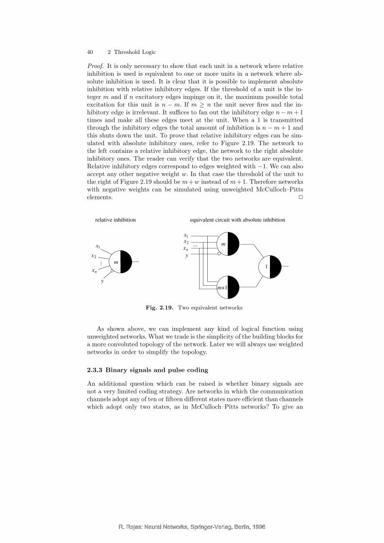
R. Rojas: Neural Networks, Springer-Verlag, Berlin, 1996
40 2 Threshold Logic
Proof. It is only necessary to show that each unit in a network where relativeinhibition is used is equivalent to one or more units in a network where ab-solute inhibition is used. It is clear that it is possible to implement absoluteinhibition with relative inhibitory edges. If the threshold of a unit is the in-teger m and if n excitatory edges impinge on it, the maximum possible totalexcitation for this unit is n − m. If m ≥ n the unit never fires and the in-hibitory edge is irrelevant. It suffices to fan out the inhibitory edge n−m+ 1times and make all these edges meet at the unit. When a 1 is transmittedthrough the inhibitory edges the total amount of inhibition is n−m+ 1 andthis shuts down the unit. To prove that relative inhibitory edges can be sim-ulated with absolute inhibitory ones, refer to Figure 2.19. The network tothe left contains a relative inhibitory edge, the network to the right absoluteinhibitory ones. The reader can verify that the two networks are equivalent.Relative inhibitory edges correspond to edges weighted with −1. We can alsoaccept any other negative weight w. In that case the threshold of the unit tothe right of Figure 2.19 should be m+w instead of m+1. Therefore networkswith negative weights can be simulated using unweighted McCulloch–Pittselements. 2
y... m
m
m+1
y
1
relative inhibition equivalent circuit with absolute inhibition
x1
x2
xn
x1
x2
xn
...
Fig. 2.19. Two equivalent networks
As shown above, we can implement any kind of logical function usingunweighted networks. What we trade is the simplicity of the building blocks fora more convoluted topology of the network. Later we will always use weightednetworks in order to simplify the topology.
2.3.3 Binary signals and pulse coding
An additional question which can be raised is whether binary signals arenot a very limited coding strategy. Are networks in which the communicationchannels adopt any of ten or fifteen different states more efficient than channelswhich adopt only two states, as in McCulloch–Pitts networks? To give an
R. Rojas: Neural Networks, Springer-Verlag, Berlin, 1996R. Rojas: Neural Networks, Springer-Verlag, Berlin, 1996
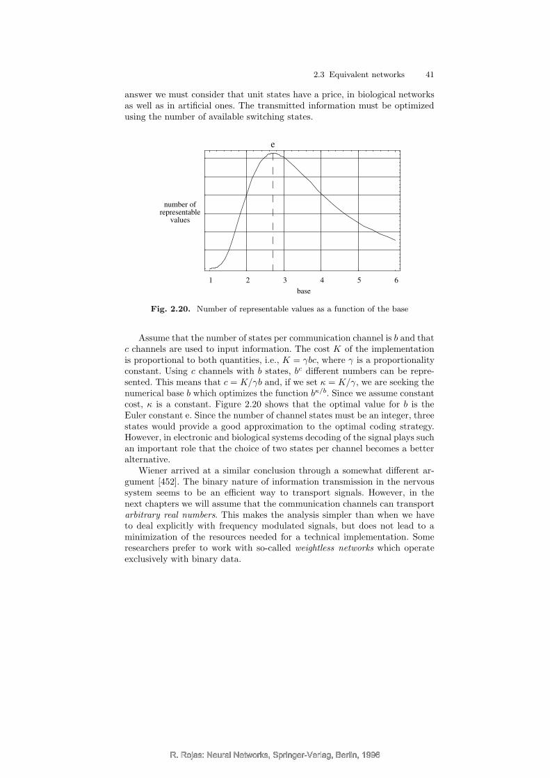
R. Rojas: Neural Networks, Springer-Verlag, Berlin, 1996
2.3 Equivalent networks 41
answer we must consider that unit states have a price, in biological networksas well as in artificial ones. The transmitted information must be optimizedusing the number of available switching states.
1 2 3 4 5 6
number ofrepresentable
values
base
e
Fig. 2.20. Number of representable values as a function of the base
Assume that the number of states per communication channel is b and thatc channels are used to input information. The cost K of the implementationis proportional to both quantities, i.e., K = γbc, where γ is a proportionalityconstant. Using c channels with b states, bc different numbers can be repre-sented. This means that c = K/γb and, if we set κ = K/γ, we are seeking thenumerical base b which optimizes the function bκ/b. Since we assume constantcost, κ is a constant. Figure 2.20 shows that the optimal value for b is theEuler constant e. Since the number of channel states must be an integer, threestates would provide a good approximation to the optimal coding strategy.However, in electronic and biological systems decoding of the signal plays suchan important role that the choice of two states per channel becomes a betteralternative.
Wiener arrived at a similar conclusion through a somewhat different ar-gument [452]. The binary nature of information transmission in the nervoussystem seems to be an efficient way to transport signals. However, in thenext chapters we will assume that the communication channels can transportarbitrary real numbers. This makes the analysis simpler than when we haveto deal explicitly with frequency modulated signals, but does not lead to aminimization of the resources needed for a technical implementation. Someresearchers prefer to work with so-called weightless networks which operateexclusively with binary data.
R. Rojas: Neural Networks, Springer-Verlag, Berlin, 1996R. Rojas: Neural Networks, Springer-Verlag, Berlin, 1996
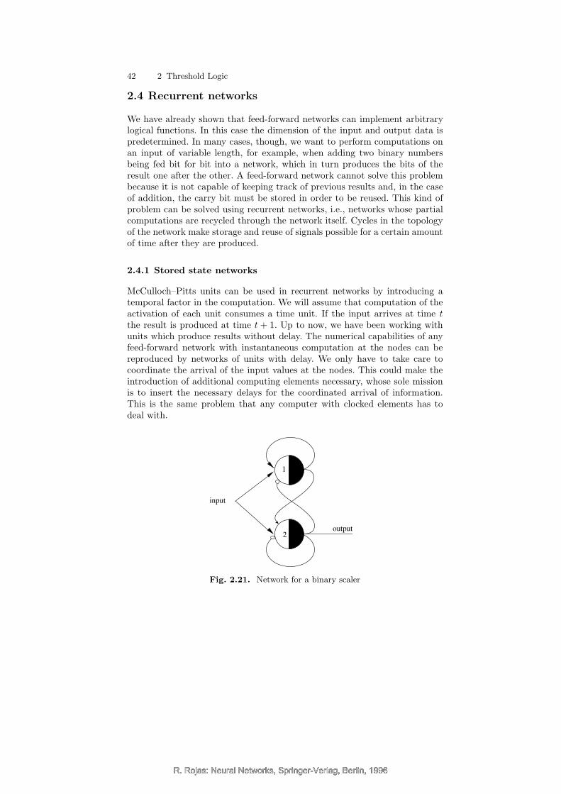
R. Rojas: Neural Networks, Springer-Verlag, Berlin, 1996
42 2 Threshold Logic
2.4 Recurrent networks
We have already shown that feed-forward networks can implement arbitrarylogical functions. In this case the dimension of the input and output data ispredetermined. In many cases, though, we want to perform computations onan input of variable length, for example, when adding two binary numbersbeing fed bit for bit into a network, which in turn produces the bits of theresult one after the other. A feed-forward network cannot solve this problembecause it is not capable of keeping track of previous results and, in the caseof addition, the carry bit must be stored in order to be reused. This kind ofproblem can be solved using recurrent networks, i.e., networks whose partialcomputations are recycled through the network itself. Cycles in the topologyof the network make storage and reuse of signals possible for a certain amountof time after they are produced.
2.4.1 Stored state networks
McCulloch–Pitts units can be used in recurrent networks by introducing atemporal factor in the computation. We will assume that computation of theactivation of each unit consumes a time unit. If the input arrives at time tthe result is produced at time t + 1. Up to now, we have been working withunits which produce results without delay. The numerical capabilities of anyfeed-forward network with instantaneous computation at the nodes can bereproduced by networks of units with delay. We only have to take care tocoordinate the arrival of the input values at the nodes. This could make theintroduction of additional computing elements necessary, whose sole missionis to insert the necessary delays for the coordinated arrival of information.This is the same problem that any computer with clocked elements has todeal with.
input
1
2output
Fig. 2.21. Network for a binary scaler
R. Rojas: Neural Networks, Springer-Verlag, Berlin, 1996R. Rojas: Neural Networks, Springer-Verlag, Berlin, 1996
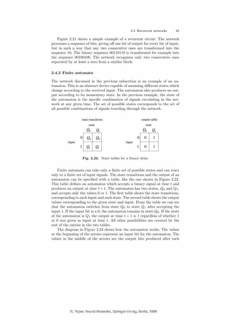
R. Rojas: Neural Networks, Springer-Verlag, Berlin, 1996
2.4 Recurrent networks 43
Figure 2.21 shows a simple example of a recurrent circuit. The networkprocesses a sequence of bits, giving off one bit of output for every bit of input,but in such a way that any two consecutive ones are transformed into thesequence 10. The binary sequence 00110110 is transformed for example intothe sequence 00100100. The network recognizes only two consecutive onesseparated by at least a zero from a similar block.
2.4.2 Finite automata
The network discussed in the previous subsection is an example of an au-tomaton. This is an abstract device capable of assuming different states whichchange according to the received input. The automaton also produces an out-put according to its momentary state. In the previous example, the state ofthe automaton is the specific combination of signals circulating in the net-work at any given time. The set of possible states corresponds to the set ofall possible combinations of signals traveling through the network.
0
1
input
state
0
1
input
state
0
0
1
1
state transitions output table
Q0 Q1
Q1Q1
Q0 Q0
Q0 Q1
Fig. 2.22. State tables for a binary delay
Finite automata can take only a finite set of possible states and can reactonly to a finite set of input signals. The state transitions and the output of anautomaton can be specified with a table, like the one shown in Figure 2.22.This table defines an automaton which accepts a binary signal at time t andproduces an output at time t+ 1. The automaton has two states, Q0 and Q1,and accepts only the values 0 or 1. The first table shows the state transitions,corresponding to each input and each state. The second table shows the outputvalues corresponding to the given state and input. From the table we can seethat the automaton switches from state Q0 to state Q1 after accepting theinput 1. If the input bit is a 0, the automaton remains in state Q0. If the stateof the automaton is Q1 the output at time t + 1 is 1 regardless of whether 1or 0 was given as input at time t. All other possibilities are covered by therest of the entries in the two tables.
The diagram in Figure 2.23 shows how the automaton works. The valuesat the beginning of the arrows represent an input bit for the automaton. Thevalues in the middle of the arrows are the output bits produced after each
R. Rojas: Neural Networks, Springer-Verlag, Berlin, 1996R. Rojas: Neural Networks, Springer-Verlag, Berlin, 1996
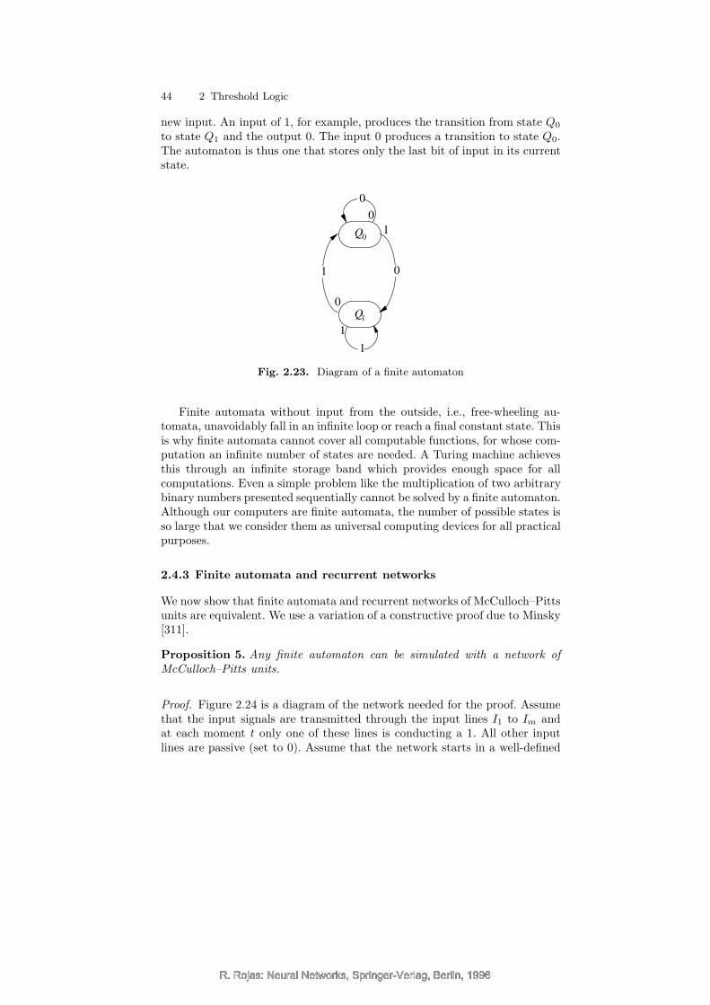
R. Rojas: Neural Networks, Springer-Verlag, Berlin, 1996
44 2 Threshold Logic
new input. An input of 1, for example, produces the transition from state Q0
to state Q1 and the output 0. The input 0 produces a transition to state Q0.The automaton is thus one that stores only the last bit of input in its currentstate.
0
0
1
1
1
1
0
0
Q0
Q1
Fig. 2.23. Diagram of a finite automaton
Finite automata without input from the outside, i.e., free-wheeling au-tomata, unavoidably fall in an infinite loop or reach a final constant state. Thisis why finite automata cannot cover all computable functions, for whose com-putation an infinite number of states are needed. A Turing machine achievesthis through an infinite storage band which provides enough space for allcomputations. Even a simple problem like the multiplication of two arbitrarybinary numbers presented sequentially cannot be solved by a finite automaton.Although our computers are finite automata, the number of possible states isso large that we consider them as universal computing devices for all practicalpurposes.
2.4.3 Finite automata and recurrent networks
We now show that finite automata and recurrent networks of McCulloch–Pittsunits are equivalent. We use a variation of a constructive proof due to Minsky[311].
Proposition 5. Any finite automaton can be simulated with a network ofMcCulloch–Pitts units.
Proof. Figure 2.24 is a diagram of the network needed for the proof. Assumethat the input signals are transmitted through the input lines I1 to Im andat each moment t only one of these lines is conducting a 1. All other inputlines are passive (set to 0). Assume that the network starts in a well-defined
R. Rojas: Neural Networks, Springer-Verlag, Berlin, 1996R. Rojas: Neural Networks, Springer-Verlag, Berlin, 1996
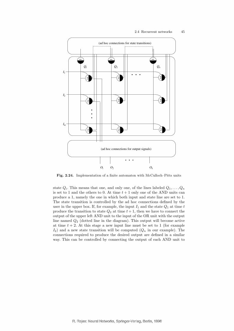
R. Rojas: Neural Networks, Springer-Verlag, Berlin, 1996
2.4 Recurrent networks 45
•
•
•
• • •
(ad hoc connections for state transitions)
(ad hoc connections for output signals)
• • •
I1
I2
Im
Q1 Q2 Qn
O1 O2 Ok
111
2 2 2
222
222
Fig. 2.24. Implementation of a finite automaton with McCulloch–Pitts units
state Qi. This means that one, and only one, of the lines labeled Q1, . . . , Qn
is set to 1 and the others to 0. At time t+ 1 only one of the AND units canproduce a 1, namely the one in which both input and state line are set to 1.The state transition is controlled by the ad hoc connections defined by theuser in the upper box. If, for example, the input I1 and the state Q1 at time tproduce the transition to state Q2 at time t+ 1, then we have to connect theoutput of the upper left AND unit to the input of the OR unit with the outputline named Q2 (dotted line in the diagram). This output will become activeat time t + 2. At this stage a new input line must be set to 1 (for exampleI2) and a new state transition will be computed (Qn in our example). Theconnections required to produce the desired output are defined in a similarway. This can be controlled by connecting the output of each AND unit to
R. Rojas: Neural Networks, Springer-Verlag, Berlin, 1996R. Rojas: Neural Networks, Springer-Verlag, Berlin, 1996
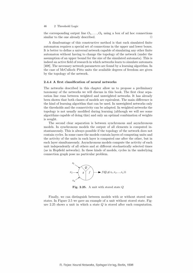
R. Rojas: Neural Networks, Springer-Verlag, Berlin, 1996
46 2 Threshold Logic
the corresponding output line O1, . . . , Ok using a box of ad hoc connectionssimilar to the one already described. 2
A disadvantage of this constructive method is that each simulated finiteautomaton requires a special set of connections in the upper and lower boxes.It is better to define a universal network capable of simulating any other finiteautomaton without having to change the topology of the network (under theassumption of an upper bound for the size of the simulated automata). This isindeed an active field of research in which networks learn to simulate automata[408]. The necessary network parameters are found by a learning algorithm. Inthe case of McCulloch–Pitts units the available degrees of freedom are givenby the topology of the network.
2.4.4 A first classification of neural networks
The networks described in this chapter allow us to propose a preliminarytaxonomy of the networks we will discuss in this book. The first clear sepa-ration line runs between weighted and unweighted networks. It has alreadybeen shown that both classes of models are equivalent. The main difference isthe kind of learning algorithm that can be used. In unweighted networks onlythe thresholds and the connectivity can be adapted. In weighted networks thetopology is not usually modified during learning (although we will see somealgorithms capable of doing this) and only an optimal combination of weightsis sought.
The second clear separation is between synchronous and asynchronousmodels. In synchronous models the output of all elements is computed in-stantaneously. This is always possible if the topology of the network does notcontain cycles. In some cases the models contain layers of computing units andthe activity of the units in each layer is computed one after the other, but ineach layer simultaneously. Asynchronous models compute the activity of eachunit independently of all others and at different stochastically selected times(as in Hopfield networks). In these kinds of models, cycles in the underlyingconnection graph pose no particular problem.
fg
x1
x2
xn
Q
f (Q, g( x1, x2,..., xn ))
Fig. 2.25. A unit with stored state Q
Finally, we can distinguish between models with or without stored unitstates. In Figure 2.5 we gave an example of a unit without stored state. Fig-ure 2.25 shows a unit in which a state Q is stored after each computation.
R. Rojas: Neural Networks, Springer-Verlag, Berlin, 1996R. Rojas: Neural Networks, Springer-Verlag, Berlin, 1996
R. Rojas: Neural Networks, Springer-Verlag, Berlin, 1996
2.5 Harmonic analysis of logical functions 47
The state Q can modify the output of the unit in the following activation.If the number of states and possible inputs is finite, we are dealing with afinite automaton. Since any finite automaton can be simulated by a networkof computing elements without memory, these units with a stored state canbe substituted by a network of McCulloch–Pitts units. Networks with stored-state units are thus equivalent to networks without stored-state units. Data isstored in the network itself and in its pattern of recursion.
It can be also shown that time varying weights and thresholds can beimplemented in a network of McCulloch–Pitts units using cycles, so that net-works with time varying weights and thresholds are equivalent to networkswith constant parameters, whenever recursion is allowed.
2.5 Harmonic analysis of logical functions
An interesting alternative for the automatic synthesis of logic functions andfor a quantification of their implementation complexity is to do an analysisof the distribution of its non-zero values using the tools of harmonic analysis.Since we can tabulate the values of a logical function in a sequence, we canthink of it as a one-dimensional function whose fundamental “frequencies” canbe extracted using the appropriate mathematical tools. We will first deal withthis problem in a totally general setting and then show that the Hadamard–Walsh transform is the tool we are looking for.
2.5.1 General expression
Assume that we are interested in expressing a function f : IRm → IR as a linearcombination of n functions f1, f2, . . . , fn using the n constants a1, a2, . . . , an
in the following form
f = a1f1 + a2f2 + · · ·+ anfn.
The domain and range of definition are the same for f and the base functions.We can determine the quadratic error E of the approximation in the whole
domain of definition V for given constants a1, . . . , an by computing
E =
∫
V
(f − (a1f1 + a2f2 + · · ·+ anfn))2dV .
Here we are assuming that f and the functions fi, i = 1, . . . , n, are integrablein its domain of definition V . Since we want to minimize the quadratic errorE we compute the partial derivatives of E with respect to a1, a2, . . . , an andset them to zero:
dE
dai= −2
∫
V
fi(f − a1f1 − a2f2 − · · · − anfn)dV = 0, for i = 1, . . . , n
R. Rojas: Neural Networks, Springer-Verlag, Berlin, 1996R. Rojas: Neural Networks, Springer-Verlag, Berlin, 1996
R. Rojas: Neural Networks, Springer-Verlag, Berlin, 1996
48 2 Threshold Logic
This leads to the following set of n equations expressed in a simplified notation:
a1
∫
fif1 + a2
∫
fif2 + · · ·+ an
∫
fifn =
∫
fif, for i = 1, . . . , n.
Expressed in matrix form the set of equations becomes:
∫f1f1
∫f1f2 · · ·
∫f1fn∫
f2f1∫f2f2
∫f2fn
.... . .
...∫fnf1
∫fnf2 · · ·
∫fnfn
a1
a2
...an
=
∫f1f∫f2f
...∫fnf
This expression is very general. The only assumption we have used is theintegrability of the partial products of the form fifj and fif . Since no specialassumptions on the integral were used, it is also possible to use a discreteversion of this equation. Assume that the function f has been defined at mpoints and let the symbol
∑fifj stand for
∑mk=1 fi(xk)fj(xk). In this case
the above expression transforms to
∑f1f1
∑f1f2 · · ·
∑f1fn∑
f2f1∑f2f2
∑f2fn
.... . .
...∑fnf1
∑fnf2 · · ·
∑fnfn
a1
a2
...an
=
∑f1f∑f2f
...∑fnf
The general formula for the polynomial approximation of m data points(x1, y1), . . . , (xm, ym) using the primitive functions x0, x1, x2, . . . , xn−1 trans-lates directly into
m∑xi · · ·
∑xn−1
i∑xi
∑x2
i
∑xn
i...
. . ....
∑xn−1
i
∑xn
i · · ·∑x2n−2
i
a1
a2
...an
=
∑yi∑xiyi
...∑xn−1
i yi
In the case of base functions that are mutually orthogonal, the integrals∫fkfj vanish when k 6= j. In this case the n × n matrix is diagonal and the
above equation becomes very simple. Assume, as in the case of the Fouriertransform, that the functions are sines and cosines of the form sin(kix) andcos(kjx). Assume that no two sine functions have the same integer wave num-ber ki and no two cosine functions the same integer wave number kj . In this
case the integral∫ 2π
0sin(kix) sin(kjx) is equal to π, whenever i = j, other-
wise it vanishes. The same is true for the cosine functions. The expressiontransforms then to
π
a1
a2
...an
=
∫f1f∫f2f
...∫fnf
R. Rojas: Neural Networks, Springer-Verlag, Berlin, 1996R. Rojas: Neural Networks, Springer-Verlag, Berlin, 1996
R. Rojas: Neural Networks, Springer-Verlag, Berlin, 1996
2.5 Harmonic analysis of logical functions 49
which is just another way of computing the coefficients for the Fourier ap-proximation of the function f .
2.5.2 The Hadamard–Walsh transform
In our case we are interested in expressing Boolean functions in terms of aset of primitive functions. We adopt bipolar coding, so that now the logicalvalue false is represented by −1 and the logical value true by 1. In the caseof n logical variables x1, . . . , xn and the logical functions defined on them, wecan use the following set of 2n primitive functions:
• The constant function (x1, . . . , xn) 7→ 1
• The
(
nk
)
monomials (x1, . . . , xn) 7→ xl1xl2 · · ·xlk , where k = 1, . . . , n and
l1, l2, . . . , lk is a set of k different indices in {1, 2, . . . , n}All these functions are mutually orthogonal. In the case of two input vari-
ables the transformation becomes:
4
a1
a2
a3
a4
=
1 1 1 1−1 1 −1 1−1 −1 1 1
1 −1 −1 1
f1f2f3f4
In the general case we compute 2n coefficients using the formula
a1
a2
...a2n
= Hn
f1f2...f2n
where the matrix Hn is defined recursively as
Hn =1
2
(Hn−1 Hn−1
−Hn−1 Hn−1
)
whereby
H1 =1
2
(1 1−1 1
)
.
The AND function can be expressed using this simple prescription as
x1 ∧ x2 =1
4(−2 + 2x1 + 2x2 + 2x1x2).
The coefficients are the result of the following computation:
a1
a2
a3
a4
=1
4
1 1 1 1−1 1 −1 1−1 −1 1 1
1 −1 −1 1
f1f2f3f4
.
R. Rojas: Neural Networks, Springer-Verlag, Berlin, 1996R. Rojas: Neural Networks, Springer-Verlag, Berlin, 1996
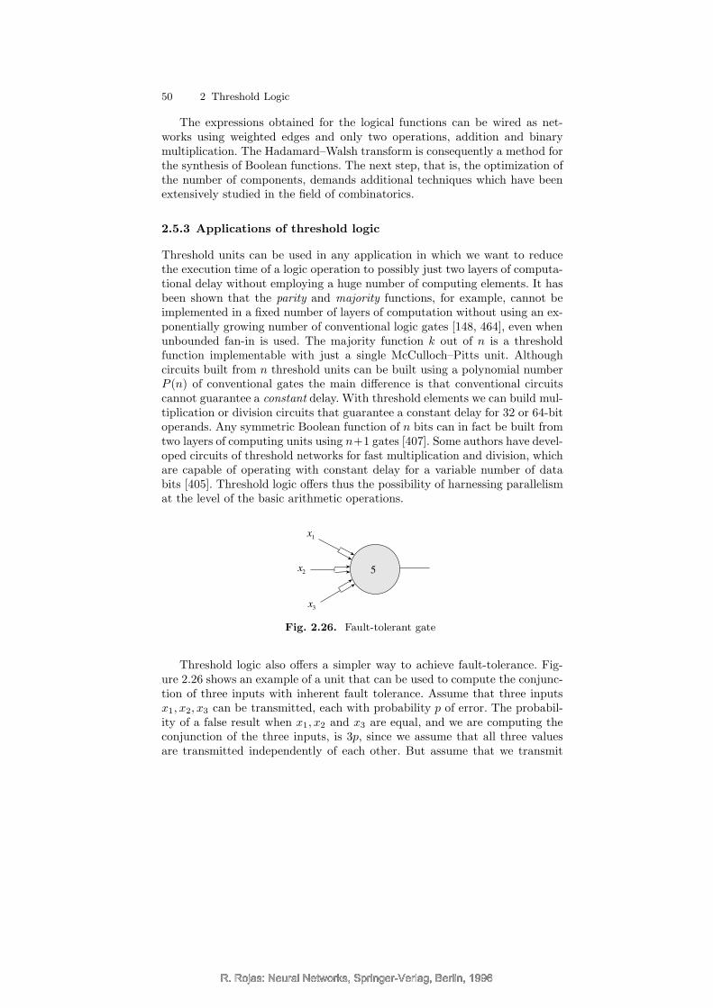
R. Rojas: Neural Networks, Springer-Verlag, Berlin, 1996
50 2 Threshold Logic
The expressions obtained for the logical functions can be wired as net-works using weighted edges and only two operations, addition and binarymultiplication. The Hadamard–Walsh transform is consequently a method forthe synthesis of Boolean functions. The next step, that is, the optimization ofthe number of components, demands additional techniques which have beenextensively studied in the field of combinatorics.
2.5.3 Applications of threshold logic
Threshold units can be used in any application in which we want to reducethe execution time of a logic operation to possibly just two layers of computa-tional delay without employing a huge number of computing elements. It hasbeen shown that the parity and majority functions, for example, cannot beimplemented in a fixed number of layers of computation without using an ex-ponentially growing number of conventional logic gates [148, 464], even whenunbounded fan-in is used. The majority function k out of n is a thresholdfunction implementable with just a single McCulloch–Pitts unit. Althoughcircuits built from n threshold units can be built using a polynomial numberP (n) of conventional gates the main difference is that conventional circuitscannot guarantee a constant delay. With threshold elements we can build mul-tiplication or division circuits that guarantee a constant delay for 32 or 64-bitoperands. Any symmetric Boolean function of n bits can in fact be built fromtwo layers of computing units using n+1 gates [407]. Some authors have devel-oped circuits of threshold networks for fast multiplication and division, whichare capable of operating with constant delay for a variable number of databits [405]. Threshold logic offers thus the possibility of harnessing parallelismat the level of the basic arithmetic operations.
5
x1
x2
x3
Fig. 2.26. Fault-tolerant gate
Threshold logic also offers a simpler way to achieve fault-tolerance. Fig-ure 2.26 shows an example of a unit that can be used to compute the conjunc-tion of three inputs with inherent fault tolerance. Assume that three inputsx1, x2, x3 can be transmitted, each with probability p of error. The probabil-ity of a false result when x1, x2 and x3 are equal, and we are computing theconjunction of the three inputs, is 3p, since we assume that all three valuesare transmitted independently of each other. But assume that we transmit
R. Rojas: Neural Networks, Springer-Verlag, Berlin, 1996R. Rojas: Neural Networks, Springer-Verlag, Berlin, 1996
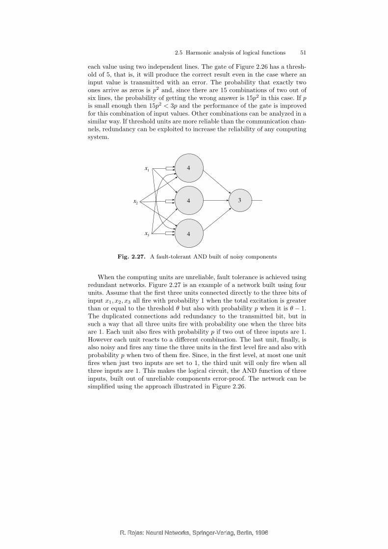
R. Rojas: Neural Networks, Springer-Verlag, Berlin, 1996
2.5 Harmonic analysis of logical functions 51
each value using two independent lines. The gate of Figure 2.26 has a thresh-old of 5, that is, it will produce the correct result even in the case where aninput value is transmitted with an error. The probability that exactly twoones arrive as zeros is p2 and, since there are 15 combinations of two out ofsix lines, the probability of getting the wrong answer is 15p2 in this case. If pis small enough then 15p2 < 3p and the performance of the gate is improvedfor this combination of input values. Other combinations can be analyzed in asimilar way. If threshold units are more reliable than the communication chan-nels, redundancy can be exploited to increase the reliability of any computingsystem.
x1
x2
x3
4
4
4
3
Fig. 2.27. A fault-tolerant AND built of noisy components
When the computing units are unreliable, fault tolerance is achieved usingredundant networks. Figure 2.27 is an example of a network built using fourunits. Assume that the first three units connected directly to the three bits ofinput x1, x2, x3 all fire with probability 1 when the total excitation is greaterthan or equal to the threshold θ but also with probability p when it is θ − 1.The duplicated connections add redundancy to the transmitted bit, but insuch a way that all three units fire with probability one when the three bitsare 1. Each unit also fires with probability p if two out of three inputs are 1.However each unit reacts to a different combination. The last unit, finally, isalso noisy and fires any time the three units in the first level fire and also withprobability p when two of them fire. Since, in the first level, at most one unitfires when just two inputs are set to 1, the third unit will only fire when allthree inputs are 1. This makes the logical circuit, the AND function of threeinputs, built out of unreliable components error-proof. The network can besimplified using the approach illustrated in Figure 2.26.
R. Rojas: Neural Networks, Springer-Verlag, Berlin, 1996R. Rojas: Neural Networks, Springer-Verlag, Berlin, 1996
R. Rojas: Neural Networks, Springer-Verlag, Berlin, 1996
52 2 Threshold Logic
2.6 Historical and bibliographical remarks
Warren McCulloch started pondering networks of artificial neurons as earlyas 1927 but had problems formulating a general, biologically plausible modelsince at that time inhibition in neurons had not yet been confirmed. He alsohad problems with the mathematical treatment of recurrent networks. Inhi-bition and recurrent pathways in the brain were confirmed in the 1930s andthis cleared the way for McCulloch’s investigations.
The McCulloch–Pitts model was proposed at a time when Norbert Wienerand Arturo Rosenblueth had started discussing the important role of feedbackin biological systems and servomechanisms [301]. Wiener and his circle hadpublished some of these ideas in 1943 [297]. Wiener’s book Cybernetics, whichwas the first best-seller in the field of Artificial Intelligence, is the most influ-ential work of this period. The word cybernetics was coined by Wiener andwas intended to underline the importance of adaptive control in living andartificial systems. Wiener himself was a polymath, capable of doing first classresearch in mathematics as well as in other fields, such as physiology andmedicine.
McCulloch and Pitts’ model was superseded rapidly by more powerful ap-proaches. Although threshold elements are, from the combinatorial point ofview, more versatile than conventional logic gates, there is a problem with theassumed unlimited fan-in. Current technology has been optimized to handle alimited number of incoming signals into a gate. A possible way of circumvent-ing the electrical difficulties could be the use of optical computing elementscapable of providing unlimited fan-in [278]. Another alternative is the defini-tion of a maximal fan-in for threshold elements that could be produced usingconventional technology. Some experiments have been conducted in this di-rection and computers have been designed using exclusively threshold logicelements. The DONUT computer of Lewis and Coates was built in the 1960susing 614 gates with a maximal fan-in of 15. The same processor built withNOR gates with a maximal fan-in of 4 required 2127 gates, a factor of ap-proximately 3.5 more components than in the former case [271].
John von Neumann [326] extensively discussed the model of McCullochand Pitts and looked carefully at its fault tolerance properties. He examinedthe question of how to build a reliable computing mechanism built of unre-liable components. However, he dealt mainly with the redundant coding ofthe units’ outputs and a canonical building block, whereas McCulloch and hiscollaborator Manuel Blum later showed how to build reliable networks out ofgeneral noisy threshold elements [300]. Winograd and Cowan generalized thisapproach by replicating modules according to the requirements of an error-correcting code [458]. They showed that sparse coding of the input signals,coupled with error correction, makes possible fault-tolerant networks even inthe presence of transmission or computational noise [94].
R. Rojas: Neural Networks, Springer-Verlag, Berlin, 1996R. Rojas: Neural Networks, Springer-Verlag, Berlin, 1996
R. Rojas: Neural Networks, Springer-Verlag, Berlin, 1996
2.6 Historical and bibliographical remarks 53
Exercises
1. Design a McCulloch–Pitts unit capable of recognizing the letter “T” dig-itized in a 10 × 10 array of pixels. Dark pixels should be coded as ones,white pixels as zeroes.
2. Build a recurrent network capable of adding two sequential streams of bitsof arbitrary finite length.
3. Show that no finite automaton can compute the product of two sequentialstreams of bits of arbitrary finite length.
4. The parity of n given bits is 1 if an odd number of them is equal to 1,otherwise it is 0. Build a network of McCulloch–Pitts units capable ofcomputing the parity function of two, three, and four given bits.
5. How many possible states can assume the binary scaler in Figure 2.21?Write the state and output tables for an equivalent finite automaton.
6. Design a network like the one shown in Figure 2.24 capable of simulatingthe finite automaton of the previous exercise.
7. Find polynomial expressions corresponding to the OR and XOR Booleanfunctions using the Hadamard–Walsh transform.
8. Show that the Hadamard–Walsh transform can be computed recursively,so that the number of multiplications becomes O(n log n), where n is thedimension of the vectors transformed (with n a power of two).
9. What is the probability of error in the case of the fault-tolerant gate shownin Figure 2.26? Consider one, two, and three faulty input bits.
10. The network in Figure 2.27 consists of unreliable computing units. Sim-plify the network. What happens if the units and the transmission channelsare unreliable?
R. Rojas: Neural Networks, Springer-Verlag, Berlin, 1996R. Rojas: Neural Networks, Springer-Verlag, Berlin, 1996
![Chapter 2 Introduction to Neural networktomczak/PDF/[Grbic]Neural...Chapter 2 Introduction to Neural network 2.1 Introduction to Artiflcial Neural Net-work Artiflcial Neural Networks](https://img.pdfslide.net/doc/110x75/5f22a87bbf292e3b5d18b33c/chapter-2-introduction-to-neural-network-tomczakpdfgrbicneural-chapter-2.jpg)


![Comparative study of LSA vs Word2vec embeddings … · Comparative study of LSA vs Word2vec embeddings in small corpora: ... 1 Introduction ... ,psychology[4,5],philology[6],cognitivescience[7]andsocial](https://img.pdfslide.net/doc/110x75/5b819a897f8b9ae87c8ca81e/comparative-study-of-lsa-vs-word2vec-embeddings-comparative-study-of-lsa-vs.jpg)