Embed Size (px)
Citation preview
Neurobiologically Inspired Control of
Engineered Flapping Flight
Soon-Jo Chung∗, Jeremiah R. Stoner†, and Michael Dorothy‡∗
Iowa State University, Ames, Iowa, 50011, USA
This article presents a new control approach for engineered flapping flight with manyinteracting degrees of freedom. This paper explores the applications of neurobiologicallyinspired control systems in the form of Central Pattern Generators (CPG) to generatewing trajectories for potential flapping flight MAVs. We present a rigorous mathematicaland control theoretic framework to design complex three dimensional motions of flappingwings. Most flapping flight demonstrators are mechanically limited in generating the wingtrajectories. Because CPGs lend themselves to more biological examples of flight, a novelrobotic model has been developed to emulate the flight of bats. This model has shoulderand leg joints totaling 10 degrees of freedom for control of wing properties. Results ofwind tunnel experiments and numerical simulation of CPG-based flight control validatethe effectiveness of the proposed neurobiologically inspired control approach.
Nomenclature
φw, ψw, θw Flapping, lead-lag, and pitch angles of each wing (left, right)xi = (ui, vi)T State vector of the i-th Hopf oscillatorf(xi; ρi) Hopf nonlinear equations in the vector form with radus ρiρi Radius of the limit cycle from the i-th Hopf oscillatorλ Common rate of convergence of Hopf oscillatorsω Common oscillation frequency of Hopf oscillators, rad/sai Amplitude bias of the i-th Hopf oscillatorR(∆ij) 2× 2 rotational transformation matrix∆ij Phase lead of the i-th Hopf oscillator from the j-thn Total number of Hopf oscillators in the CPG networkIk Identity matrix ∈ Rk×kk Coupling gain of the coupled Hopf oscillatorskr Reduced frequency of the flapping wing` Contraction rate of the virtual nonlinear systemG Original Laplacian matrix with rotational transformation ∈ R2n×2n
L Graph Laplacian matrix ∈ R2n×2n
V Matrix of orthonormal eigenvectors of L without the ones vector ∈ R2n×2(n−1)
λmin(·), λmax(·) Minimum or maximum eigenvalues of the matrixxb = (xb, yb, zb) Vehicle body frame coordinatesxw = (xw, yw, zs) Wing frame coordinates (left, right)xs = (xs, ys, zs) Stroke plane frame coordinatesR Wing span of a single wing, mr Wing span coordinate value r ∈ [0, R] of the wing blade elementαw(r, t) Local angle of attack of the wing blade element
∗Assistant Professor of Aerospace Engineering, Senior Member AIAA, Phone: 515-294-5459, [email protected].†Graduate Research Assistant, Aerospace Engineering, [email protected].‡Research Assistant, Aerospace Engineering, [email protected].
1 of 29
American Institute of Aeronautics and Astronautics
AIAA Infotech@Aerospace Conference <br>and <br>AIAA Unmanned...Unlimited Conference 6 - 9 April 2009, Seattle, Washington
AIAA 2009-1929
Copyright © 2009 by the American Institute of Aeronautics and Astronautics, Inc. All rights reserved.
Dow
nloa
ded
by U
NIV
ER
SIT
Y O
F IL
LIN
OIS
on
Mar
ch 2
0, 2
013
| http
://ar
c.ai
aa.o
rg |
DO
I: 1
0.25
14/6
.200
9-19
29
βw(r, t) Local direction of the wind in the wing frameV∞ Speed of the vehicle, without the relative wind, m/sVr Local wind speed of the wing blade element, m/sCL(αw), CD(αw) Local lift and drag coefficients of the blade elementFwx, Fwz Total aerodynamic forces of each wing in the x and z directions of the wing frameF = (Fx, Fy, Fz)T Total aerodynamic forces from the wing in the body frame (left, right)d = (dx, dy, dz)T Location of the stroke and wing frames with respect to the body frameTbs, Tsw Angular transformation matrixαx, αy Angle of attack and slide-slip angle of the vehicle body, rad/sΘs Stroke plane inclination angle from the vertical lineTbe Directional cosine matrix of Euler angles ∈ R3×3
Ωb = (p, q, r)T Body angular rate, rad/s(φb, θb, ψb) Euler angles of the vehicle body with respect to the inertial frame, radM = (Mx,My,Mz) Total aerodynamic moments from each wing, NmVb = (Vbx, Vby, Vbz)T Vehicle velocity vector in the body frameFg = (0, 0,mg)T Gravitational force vector in the inertial frameA = (Ax, Ay, Az)T Additional forces generated by the body (fuselage) and the tailIb Inertia matrix ∈ R3×3 , kgm2
B = (Bx, By, Bz)T Additional aerodynamic moments from the body and the tailSubscripti Variable number of the coupled Hopf nonlinear oscillatorsR, L Right or left wingb, s, w Body, stroke, and wing frame
I. Introduction
Engineered flapping flight holds promise for creating biomimetic micro aerial vehicles (MAVs) flying in lowReynolds number regimes (Re< 105) where rigid fixed wings drop substantially in aerodynamic performance.MAVs are typically classified as having maximum dimensions of 15 cm and flying at a nominal speed of 1–20m/s in tight urban environments.1,2 Although natural flyers such as bats, birds, and insects have captured theimaginations of scientists and engineers for centuries, the maneuvering characteristics of man-made aircraftare nowhere near the agility and efficiency of animal flight.3–5 Such highly maneuverable MAVs, equippedwith intelligent sensors, will make paradigm-shifting advances in monitoring of critical infrastructures suchas power grids, bridges, and borders, as well as in intelligence, surveillance, and reconnaissance applications.The successful reverse-engineering of flapping flight will potentially result in a transformative innovation inaircraft design, which has been dominated by fixed-wing airplanes.
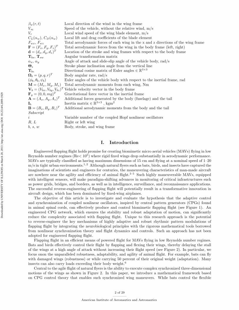
The objective of this article is to investigate and evaluate the hypothesis that the adaptive controland synchronization of coupled nonlinear oscillators, inspired by central pattern generators (CPGs) foundin animal spinal cords, can effectively produce and control biomimetic flapping flight (see Figure 1). Anengineered CPG network, which ensures the stability and robust adaptation of motion, can significantlyreduce the complexity associated with flapping flight. Unique to this research approach is the potentialto reverse-engineer the key mechanisms of highly adaptive and robust rhythmic pattern modulations offlapping flight by integrating the neurobiological principles with the rigorous mathematical tools borrowedfrom nonlinear synchronization theory and flight dynamics and controls. Such an approach has not beenadopted for engineered flapping flight.
Flapping flight in an efficient means of powered flight for MAVs flying in low Reynolds number regimes.Bats and birds effectively control their flight by flapping and flexing their wings, thereby delaying the stallof the wings at a high angle of attack without increasing their flight speed (see Figure 2). In particular, wefocus onon the unparalleled robustness, adaptability, and agility of animal flight. For example, bats can flywith damaged wings (robustness) or while carrying 50 percent of their original weight (adaptation). Manyinsects can also carry loads exceeding their body weight.6
Central to the agile flight of natural flyers is the ability to execute complex synchronized three-dimensionalmotions of the wings as shown in Figure 2. In this paper, we introduce a mathematical framework basedon CPG control theory that enables such synchronized wing maneuvers. While bats control the flexible
2 of 29
American Institute of Aeronautics and Astronautics
Dow
nloa
ded
by U
NIV
ER
SIT
Y O
F IL
LIN
OIS
on
Mar
ch 2
0, 2
013
| http
://ar
c.ai
aa.o
rg |
DO
I: 1
0.25
14/6
.200
9-19
29
Leg
Shoulder
Elbow
Wrist
Fingers
Wind
Wrist
Elbow
Shoulder
Hand Hand
Legs
Joint Angles and Muscle StretchBody acceleration
and angular rate by IMU; echolocation by sonar; and vision by CCD
Cutaneous hairy
sensors on the wings
Amp.
Freq.
Phase
Coupling
Gains
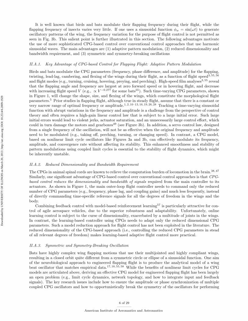
Figure 1. Proposed hierarchical control structures with the main controller and the CPG network. The outer-loopflight control modulates the rhythmic patterns (frequency, amplitude, phase lag, coupling gains) of the CPG network,without the need for directly controlling a multitude of joints.
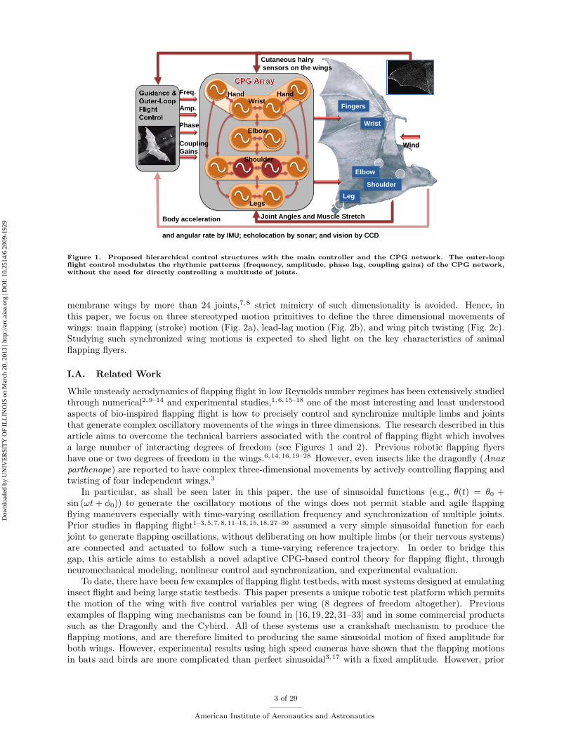
membrane wings by more than 24 joints,7,8 strict mimicry of such dimensionality is avoided. Hence, inthis paper, we focus on three stereotyped motion primitives to define the three dimensional movements ofwings: main flapping (stroke) motion (Fig. 2a), lead-lag motion (Fig. 2b), and wing pitch twisting (Fig. 2c).Studying such synchronized wing motions is expected to shed light on the key characteristics of animalflapping flyers.
I.A. Related Work
While unsteady aerodynamics of flapping flight in low Reynolds number regimes has been extensively studiedthrough numerical2,9–14 and experimental studies,1,6, 15–18 one of the most interesting and least understoodaspects of bio-inspired flapping flight is how to precisely control and synchronize multiple limbs and jointsthat generate complex oscillatory movements of the wings in three dimensions. The research described in thisarticle aims to overcome the technical barriers associated with the control of flapping flight which involvesa large number of interacting degrees of freedom (see Figures 1 and 2). Previous robotic flapping flyershave one or two degrees of freedom in the wings.6,14,16,19–28 However, even insects like the dragonfly (Anaxparthenope) are reported to have complex three-dimensional movements by actively controlling flapping andtwisting of four independent wings.3
In particular, as shall be seen later in this paper, the use of sinusoidal functions (e.g., θ(t) = θ0 +sin (ωt+ φ0)) to generate the oscillatory motions of the wings does not permit stable and agile flappingflying maneuvers especially with time-varying oscillation frequency and synchronization of multiple joints.Prior studies in flapping flight1–3,5, 7, 8, 11–13,15,18,27–30 assumed a very simple sinusoidal function for eachjoint to generate flapping oscillations, without deliberating on how multiple limbs (or their nervous systems)are connected and actuated to follow such a time-varying reference trajectory. In order to bridge thisgap, this article aims to establish a novel adaptive CPG-based control theory for flapping flight, throughneuromechanical modeling, nonlinear control and synchronization, and experimental evaluation.
To date, there have been few examples of flapping flight testbeds, with most systems designed at emulatinginsect flight and being large static testbeds. This paper presents a unique robotic test platform which permitsthe motion of the wing with five control variables per wing (8 degrees of freedom altogether). Previousexamples of flapping wing mechanisms can be found in [16, 19, 22, 31–33] and in some commercial productssuch as the Dragonfly and the Cybird. All of these systems use a crankshaft mechanism to produce theflapping motions, and are therefore limited to producing the same sinusoidal motion of fixed amplitude forboth wings. However, experimental results using high speed cameras have shown that the flapping motionsin bats and birds are more complicated than perfect sinusoidal3,17 with a fixed amplitude. However, prior
3 of 29
American Institute of Aeronautics and Astronautics
Dow
nloa
ded
by U
NIV
ER
SIT
Y O
F IL
LIN
OIS
on
Mar
ch 2
0, 2
013
| http
://ar
c.ai
aa.o
rg |
DO
I: 1
0.25
14/6
.200
9-19
29
(a) flapping (φw) (b) lead-lag (ψw) (c) twisting (θw) and cambering)
Figure 2. Basic wing movements of bats (pictures from [18]). Except for cambering, birds exhibit similar wing move-ments. Twisting (pitching) changes the effective angle of attack while cambering changes the aerodynamic efficiency.The fingers and hind legs control the tension of the flexible membrane wings, which distinguish bats from birds.5
systems do not allow changes in flapping stroke amplitude as well as stroke frequency. Further, multipleparameters of the flapping change depending on flight conditions such as the pitch and the lead-lag angles(see Fig. 2). The amplitude of the wing beats varies, as does the phase relationship between the differentmovements of the wing.
The paper is organized as follows. We illustrate the fundamentals and advantages of the CPG basedcontrol for engineered flapping flight in Section II. We present a mathematical and control theoretic formu-lation of synchronized motions of multiple joints in the wings and body in Section II.B in the context ofcombining the CPG network with the kinematic modeling of three-dimensional multi-joint wings presentedin Section III. We present results of simulations with with multijoint coordination that go beyond previousstudies on robotic flapping flyers with a single-joint wing beating in Section IV. Further, we introduce aunique robotic flapping flying testbed in Section V and its experimental results that validate the proposedcontrol strategy. We understand the challenges associated with building lightweight actuators to truly realizethe potential of three dimensional wing maneuvers. We present the fundamental neurobiologically inspiredcontrol theory that can further contribute to engineered flapping flight, once such light-weight actuatorsbecome available in the future. In the meantime, we show how the multi-joint robotic bat testbed driven byCPG control can further enhance our understanding of biomimmetic flapping flight.
II. Fundamentals of Neurobiologically Inspired Control
This article reports the first investigation of CPG models by using coupled limit cycle oscillators forthe purpose of controlled engineered flapping flight. The central pattern generators of animals are neuralnetworks that can endogenously (i.e., without rhythmic sensory or central input) produce coordinated pat-terns of rhythmic outputs. Hence, CPGs are believed to reduce the computation burden of the brain. Asseen in Fig. 1, the central controller, similar to the brain of an animal, can stabilize the vehicle dynamicsby commanding a reduced number of variables such as the frequency and phase difference of the oscillatorsinstead of directly controlling multiple joints. The existence of CPGs has been confirmed by biologists.34–42
Interestingly, the first modern evidence of CPGs came from the experiments with flapping flying locusts43
rather than walking or swimming animals. Experiments with limbed vertebrates have also shown that indi-vidual limbs can produce rhythmic movements endogenously.38,44 Such empirical data have been interpretedas evidence that each limb has its own CPGs that can behave in a self-sustained way. However, sensoryfeedback is also known to play a crucial role in altering motor patterns38,45 to cope with environmentalperturbations. Incorporation of sensory feedback into the CPG model has been presented in [46] for a turtlerobot.
The most popular animal model for CPGs has been the lamprey, a primitive eel-like fish.47 While therobotics community eagerly embraced the concept of CPG models for swimming or walking robots,46,48–50
this work reports the first CPG-based control for flapping flight. The use of nonlinear oscillators for insectflapping flight has also been suggested by some biologists.29,30 Clearly, flapping flight is technically morechallenging to mimic than swimming and walking, due to its uncompromising aerodynamic characteristics.
II.A. Robust and Adaptive Flapping Pattern Generation by CPGs
Our neurobiologically inspired approach centers on deriving an effective mathematical model of CPGs basedon coupled nonlinear limit cycle dynamics. Once neurons form reciprocally inhibiting relations, they oscillateand spike periodically.46 An abstract mathematical model of complicated neuron models can be obtained by
4 of 29
American Institute of Aeronautics and Astronautics
Dow
nloa
ded
by U
NIV
ER
SIT
Y O
F IL
LIN
OIS
on
Mar
ch 2
0, 2
013
| http
://ar
c.ai
aa.o
rg |
DO
I: 1
0.25
14/6
.200
9-19
29
−80 −60 −40 −20 0 20 40 60−60
−40
−20
0
20
40
60
Angle u [deg]
Ang
le v
(a)
0 10 20 30 40 50 60 70 80 90 100−1
0
1CPG based Control
0 10 20 30 40 50 60 70 80 90 100−1
0
1Sine based Control
0 10 20 30 40 50 60 70 80 90 1000
2
4
Fre
q [r
ad/s
]
Time [s]
(b)
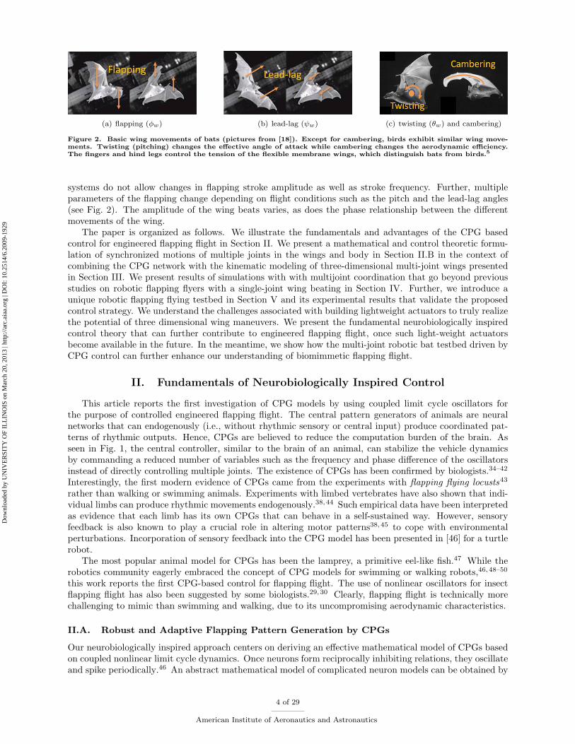
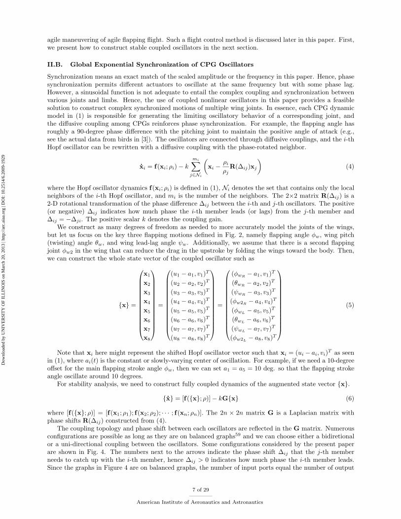
Figure 3. (a) Phase portrait of multiple Hopf oscillators synchronizing (b)CPG-based control using Hopf limit cycle(first row) and sin(ωt) control (second row) with time-varying ω(t) (third row). The Hopf limit cycle shows a muchsmoother transition. This is true for amplitude and bias changes as well.
coupled nonlinear limit cycles that essentially exhibit the rhythmic behaviors of coupled neuronal networks.In the field of nonlinear dynamics, a limit cycle is defined as an isolated closed trajectory that exhibitsself-sustained oscillation.51,52 If stable, small perturbations (initial conditions) will be forgotten and thetrajectories will converge to the limit cycle (see Figures 3a and 3b). This superior robustness makes a limitcycle an ideal simplified dynamic model of CPGs.
In the present paper, we use the following limit-cycle model called the Hopf oscillator, named after theHopf bifurcation model:
d
dt
(u− av
)=
−λ( (u−a)2+v2
ρ2 − 1)
−ω(t)
ω(t) −λ(
(u−a)2+v2
ρ2 − 1)(u− a
v
)+ u(t)
Equivalently, x = f(x; ρ) + u(t), with x = (u− a, v)T
(1)
where the λ > 0 denotes the convergence rate to the symmetric limit circle of the radius ρ > 0 and u(t)is an external or coupling input. Indeed, for a single Hopf oscillator with u(t) = 0, a Lyapunov function
V =(
(u−a)2+v2
ρ2 − 1)2
can be used to prove global asymptotic stability to the limit circle. For coupled Hopfoscillators, the stability proof is much more involved and discussed in Section II.B.
Also, the possibly time-varying parameter ω(t) > 0 determines the oscillation frequency of the limit circle.Note that a constant or slowly varying a sets the bias to the limit cycle such that u(t) = ρ cos (ωt+ δ) + aand v(t) = ρ sin (ωt+ δ) on a circle. The variable output u(t) is then used to to generate an oscillatory signalfor the corresponding joint. Since it does not change the results of the stability proof, we will drop this bias”a” in the equations. Then, the output variable to generate the desired oscillatory motion of each joint isthe first state u from the Hopf oscillator model in (1).
In order to construct an artificial CPG network, some prior work uses a discrete nonlinear equation thatdescribes spiking and spiking-bursting of a neuron model.48 On the other hand, the Hopf oscillator has beena popular dynamic model of the engineered CPG arrays (e.g., see the salamander robot49,49 and the turtlerobot46). The stability of coupled Hopf oscillators has been extensively investigated in [46,53,54]. One niceproperty of the Hopf oscillator in (1) is that its limit cycle is a symmetric circle as opposed to Van der Pol34
or Rayleigh oscillators.51 Further, as shall been seen later, the following two properties are exploited in thestability proof of phase synchronization:
f(R(∆)x; ρ) = R(∆)f(x; ρ) R(∆) =
[cos ∆ − sin ∆sin ∆ cos ∆
](2)
where R(∆) ∈ SO(2) is a 2D rotational transformation such that R(−∆) = −R(∆) = R−1(∆) = RT (∆).Also, its scaling factor can be expressed as
f(gx; ρ) = gf(x; ρ/g) (3)
5 of 29
American Institute of Aeronautics and Astronautics
Dow
nloa
ded
by U
NIV
ER
SIT
Y O
F IL
LIN
OIS
on
Mar
ch 2
0, 2
013
| http
://ar
c.ai
aa.o
rg |
DO
I: 1
0.25
14/6
.200
9-19
29
It is well known that birds and bats modulate their flapping frequency during their flight, while theflapping frequency of insects varies very little. If one uses a sinusoidal function φw = sin(ωt) to generateoscillatory patterns of the wing, the frequency variation for the purpose of flight control is not permitted asseen in Fig. 3b. This salient point is further illustrated in this section. The following advantages motivatethe use of more sophisticated CPG-based control over conventional control approaches that use harmonicsinusoidal waves. The main advantages are (1) adaptive pattern modulation, (2) reduced dimensionality andbandwidth requirement, and (3) symmetric and symmetry-breaking oscillations
II.A.1. Key Advantage of CPG-based Control for Flapping Flight: Adaptive Pattern Modulation
Birds and bats modulate the CPG parameters (frequency, phase difference, and amplitude) for the flapping,twisting, lead-lag, cambering, and flexing of the wings during their flight, as a function of flight speed3,55,56
and flight modes (e.g., turning, cruising, hovering, preying, and perching). High-speed film analyses3,55 revealthat the flapping angle and frequency are largest at zero forward speed or in hovering flight, and decreasewith increasing flight speed V (e.g., ∝ V −0.277 for some bats55). Such time-varying CPG parameters, shownin Figure 1, will change the shape, size, and flexing of the wings, which constitute the morphological flightparameters.5 Prior studies in flapping flight, although true in steady flight, assume that there is a constant orvery narrow range of optimal frequency or amplitude.1,2, 10–13,16,19,26,28 Tracking a time-varying sinusoidalfunction with abrupt variations in the frequency and amplitude is a challenge from the perspective of controltheory and often requires a high-gain linear control law that is subject to a large initial error. Such largeinitial errors would lead to violent jerks, actuator saturation, and an unnecessarily large control effort, whichcould in turn damage the motors and gearboxes49 (see Figure 3b). In addition, a servo control law, designedfrom a single frequency of the oscillation, will not be as effective when the original frequency and amplitudeneed to be modulated (e.g., taking off, perching, turning, or changing speed). In contrast, a CPG model,based on nonlinear limit cycle oscillators like Figures 3a and 3b, can effectively modulate its frequency,amplitude, and convergence rate without affecting its stability. This enhanced smoothness and stability ofpattern modulations using coupled limit cycles is essential to the stability of flight dynamics, which mightbe inherently unstable.
II.A.2. Reduced Dimensionality and Bandwidth Requirement
The CPGs in animal spinal cords are known to relieve the computation burden of locomotion in the brain.38,47
Similarly, one significant advantage of CPG-based control over conventional control approaches is that CPG-based control reduces the dimensionality and bandwidth of signals required from the main controller to itsactuators. As shown in Figure 1, the main outer-loop flight controller needs to command only the reducednumber of CPG parameters (e.g., frequency, phase lag, and coupling gains) and much less frequently, insteadof directly commanding time-specific reference signals for all the degrees of freedom in the wings and thebody.
Combining feedback control with model-based reinforcement learning57 is particularly attractive for con-trol of agile aerospace vehicles, due to the superior robustness and adaptability. Unfortunately, onlinelearning control is subject to the curse of dimensionality, exacerbated by a multitude of joints in the wings.In contrast, the learning-based controller using CPGs needs to adapt only the reduced dimensional CPGparameters. Such a model reduction approach for flight control has not been exploited in the literature. Thereduced dimensionality of the CPG-based approach (i.e., controlling the reduced CPG parameters in steadof all relevant degrees of freedom) makes learning-based adaptive flight control more practical.
II.A.3. Symmetric and Symmetry-Breaking Oscillation
Bats have highly complex wing flapping motions that use their multijointed and highly compliant wings,resulting in a closed orbit quite different from a symmetric circle or ellipse of a sinusoidal function. One aimof the neurobiological approach to engineered flapping flight is to produce the analytical model of a wingbeat oscillator that matches empirical data.17,18,55,58 While the benefits of nonlinear limit cycles for CPGmodels are articulated above, deriving an effective CPG model for engineered flapping flight has been largelyan open problem (e.g., limit cycle dynamics, network topology, and how to integrate input and feedbacksignals). The key research issues include how to ensure the amplitude or phase synchronization of multiplecoupled CPG oscillators and how to opportunistically break the symmetry of the oscillators for performing
6 of 29
American Institute of Aeronautics and Astronautics
Dow
nloa
ded
by U
NIV
ER
SIT
Y O
F IL
LIN
OIS
on
Mar
ch 2
0, 2
013
| http
://ar
c.ai
aa.o
rg |
DO
I: 1
0.25
14/6
.200
9-19
29
agile maneuvering of agile flapping flight. Such a flight control method is discussed later in this paper. First,we present how to construct stable coupled oscillators in the next section.
II.B. Global Exponential Synchronization of CPG Oscillators
Synchronization means an exact match of the scaled amplitude or the frequency in this paper. Hence, phasesynchronization permits different actuators to oscillate at the same frequency but with some phase lag.However, a sinusoidal function is not adequate to entail the complex coupling and synchronization betweenvarious joints and limbs. Hence, the use of coupled nonlinear oscillators in this paper provides a feasiblesolution to construct complex synchronized motions of multiple wing joints. In essence, each CPG dynamicmodel in (1) is responsible for generating the limiting oscillatory behavior of a corresponding joint, andthe diffusive coupling among CPGs reinforces phase synchronization. For example, the flapping angle hasroughly a 90-degree phase difference with the pitching joint to maintain the positive angle of attack (e.g.,see the actual data from birds in [3]). The oscillators are connected through diffusive couplings, and the i-thHopf oscillator can be rewritten with a diffusive coupling with the phase-rotated neighbor.
xi = f(xi; ρi)− kmi∑j∈Ni
(xi −
ρiρj
R(∆ij)xj
)(4)
where the Hopf oscillator dynamics f(xi; ρi) is defined in (1), Ni denotes the set that contains only the localneighbors of the i-th Hopf oscillator, and mi is the number of the neighbors. The 2×2 matrix R(∆ij) is a2-D rotational transformation of the phase difference ∆ij between the i-th and j-th oscillators. The positive(or negative) ∆ij indicates how much phase the i-th member leads (or lags) from the j-th member and∆ij = −∆ji. The positive scalar k denotes the coupling gain.
We construct as many degrees of freedom as needed to more accurately model the joints of the wings,but let us focus on the key three flapping motions defined in Fig. 2, namely flapping angle φw, wing pitch(twisting) angle θw, and wing lead-lag angle ψw. Additionally, we assume that there is a second flappingjoint φw2 in the wing that can reduce the drag in the upstroke by folding the wings toward the body. Then,we can construct the whole state vector of the coupled oscillator such as
x =
x1
x2
x3
x4
x5
x6
x7
x8
=
(u1 − a1, v1)T
(u2 − a2, v2)T
(u3 − a3, v3)T
(u4 − a4, v4)T
(u5 − a5, v5)T
(u6 − a6, v6)T
(u7 − a7, v7)T
(u8 − a8, v8)T
=
(φwR− a1, v1)T
(θwR− a2, v2)T
(ψwR− a3, v3)T
(φw2R− a4, v4)T
(φwL− a5, v5)T
(θwL− a6, v6)T
(ψwL− a7, v7)T
(φw2L− a8, v8)T
(5)
Note that xi here might represent the shifted Hopf oscillator vector such that xi = (ui − ai, vi)T as seenin (1), where ai(t) is the constant or slowly-varying center of oscillation. For example, if we need a 10-degreeoffset for the main flapping stroke angle φw, then we can set a1 = a5 = 10 deg. so that the flapping strokeangle oscillate around 10 degrees.
For stability analysis, we need to construct fully coupled dynamics of the augmented state vector x.
x = [f(x; ρ)]− kGx (6)
where [f(x; ρ)] = [f(x1; ρ1); f(x2; ρ2); · · · ; f(xn; ρn)]. The 2n × 2n matrix G is a Laplacian matrix withphase shifts R(∆ij) constructed from (4).
The coupling topology and phase shift between each oscillators are reflected in the G matrix. Numerousconfigurations are possible as long as they are on balanced graphs59 and we can choose either a bidiretionalor a uni-directional coupling between the oscillators. Some configurations considered by the present paperare shown in Fig. 4. The numbers next to the arrows indicate the phase shift ∆ij that the j-th memberneeds to catch up with the i-th member, hence ∆ij > 0 indicates how much phase the i-th member leads.Since the graphs in Figure 4 are on balanced graphs, the number of input ports equal the number of output
7 of 29
American Institute of Aeronautics and Astronautics
Dow
nloa
ded
by U
NIV
ER
SIT
Y O
F IL
LIN
OIS
on
Mar
ch 2
0, 2
013
| http
://ar
c.ai
aa.o
rg |
DO
I: 1
0.25
14/6
.200
9-19
29
φφΔ Δ0°
Rwφ
θ
2RwφLwφ
θ
2Lwφ21Δ65Δ
75−Δ 31−Δ0°
Rwθ
Rwψ
Lwθ
Lwψ 31 21Δ −Δ75 65Δ −Δ
0°0°
RwφLwφ75−Δ 0°0° 31−Δ
Rwφ
wθ
2RwφLwφ
wθ
2Lwφ21Δ65Δ
0°0°
0° 31
Rw
Rwψ
Lw
31 21Δ −Δ75 65Δ −Δ00
Lwψ 75 31Δ −ΔΔ −Δ31 75Δ Δ
(a) Configuration A
φφ 90°0°
Rwφ
θ
2RwφLwφ
θ
2Lwφ 90°90°90° 90°
0°
Rwθ
Rwψ
Lwθ
Lwψ 180°180°
0°0°
RwφLwφ5,7−Δ 1,3−Δ0°0° Rwφ
wθ
2RwφLwφ
wθ
2Lwφ1,2Δ5,6Δ
, ,
0°0°
0°
Rw
Rwψ
Lw1,3 1,2Δ −Δ
5,7 5,6Δ −Δ00
Lwψ 5,7 1,3Δ −ΔΔ −Δ1,3 5,7Δ Δ
(b) Symmetric Configuration A
φφΔ Δ0°
Rwφ
θ
2RwφLwφ
θ
2Lwφ21Δ65Δ
75−Δ 31−Δ0°
Rwθ
Rwψ
Lwθ
Lwψ 31 21Δ −Δ75 65Δ −Δ
0°0°
RwφLwφ75−Δ 0°0° 31−Δ
Rwφ
wθ
2RwφLwφ
wθ
2Lwφ21Δ65Δ
0°0°
0° 31
Rw
Rwψ
Lw
31 21Δ −Δ75 65Δ −Δ00
Lwψ 75 31Δ −ΔΔ −Δ31 75Δ Δ
(c) Configuration B
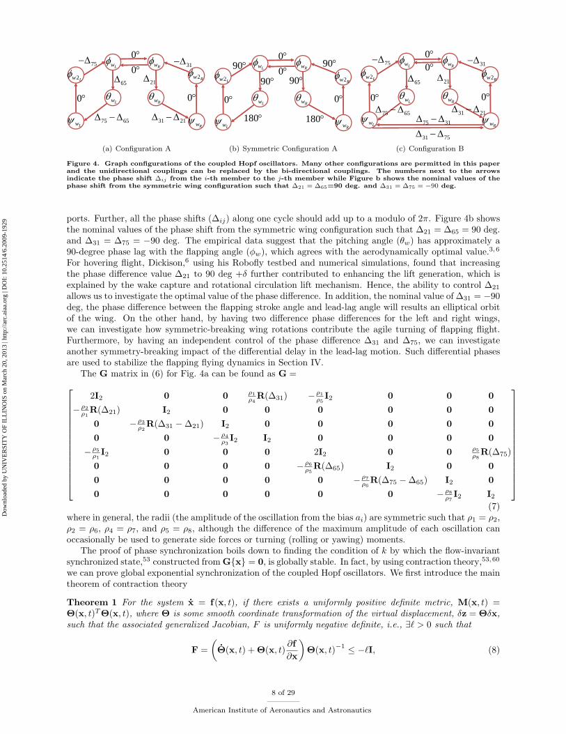
Figure 4. Graph configurations of the coupled Hopf oscillators. Many other configurations are permitted in this paperand the unidirectional couplings can be replaced by the bi-directional couplings. The numbers next to the arrowsindicate the phase shift ∆ij from the i-th member to the j-th member while Figure b shows the nominal values of thephase shift from the symmetric wing configuration such that ∆21 = ∆65=90 deg. and ∆31 = ∆75 = −90 deg.
ports. Further, all the phase shifts (∆ij) along one cycle should add up to a modulo of 2π. Figure 4b showsthe nominal values of the phase shift from the symmetric wing configuration such that ∆21 = ∆65 = 90 deg.and ∆31 = ∆75 = −90 deg. The empirical data suggest that the pitching angle (θw) has approximately a90-degree phase lag with the flapping angle (φw), which agrees with the aerodynamically optimal value.3,6
For hovering flight, Dickison,6 using his Robofly testbed and numerical simulations, found that increasingthe phase difference value ∆21 to 90 deg +δ further contributed to enhancing the lift generation, which isexplained by the wake capture and rotational circulation lift mechanism. Hence, the ability to control ∆21
allows us to investigate the optimal value of the phase difference. In addition, the nominal value of ∆31 = −90deg, the phase difference between the flapping stroke angle and lead-lag angle will results an elliptical orbitof the wing. On the other hand, by having two difference phase differences for the left and right wings,we can investigate how symmetric-breaking wing rotations contribute the agile turning of flapping flight.Furthermore, by having an independent control of the phase difference ∆31 and ∆75, we can investigateanother symmetry-breaking impact of the differential delay in the lead-lag motion. Such differential phasesare used to stabilize the flapping flying dynamics in Section IV.
The G matrix in (6) for Fig. 4a can be found as G =
2I2 0 0 ρ1ρ4
R(∆31) −ρ1ρ5 I2 0 0 0
−ρ2ρ1 R(∆21) I2 0 0 0 0 0 0
0 −ρ3ρ2 R(∆31 −∆21) I2 0 0 0 0 0
0 0 −ρ4ρ3 I2 I2 0 0 0 0
−ρ5ρ1 I2 0 0 0 2I2 0 0 ρ5ρ8
R(∆75)0 0 0 0 −ρ6ρ5 R(∆65) I2 0 0
0 0 0 0 0 −ρ7ρ6 R(∆75 −∆65) I2 0
0 0 0 0 0 0 −ρ8ρ7 I2 I2
(7)
where in general, the radii (the amplitude of the oscillation from the bias ai) are symmetric such that ρ1 = ρ2,ρ2 = ρ6, ρ4 = ρ7, and ρ5 = ρ8, although the difference of the maximum amplitude of each oscillation canoccasionally be used to generate side forces or turning (rolling or yawing) moments.
The proof of phase synchronization boils down to finding the condition of k by which the flow-invariantsynchronized state,53 constructed from Gx = 0, is globally stable. In fact, by using contraction theory,53,60
we can prove global exponential synchronization of the coupled Hopf oscillators. We first introduce the maintheorem of contraction theory
Theorem 1 For the system x = f(x, t), if there exists a uniformly positive definite metric, M(x, t) =Θ(x, t)TΘ(x, t), where Θ is some smooth coordinate transformation of the virtual displacement, δz = Θδx,such that the associated generalized Jacobian, F is uniformly negative definite, i.e., ∃` > 0 such that
F =(
Θ(x, t) + Θ(x, t)∂f∂x
)Θ(x, t)−1 ≤ −`I, (8)
8 of 29
American Institute of Aeronautics and Astronautics
Dow
nloa
ded
by U
NIV
ER
SIT
Y O
F IL
LIN
OIS
on
Mar
ch 2
0, 2
013
| http
://ar
c.ai
aa.o
rg |
DO
I: 1
0.25
14/6
.200
9-19
29
then all system trajectories converge globally to a single trajectory exponentially fast regardless of the initialconditions, with a global exponential convergence rate of the largest eigenvalues of the symmetric part of F.
Such a system is said to be contracting.
Proof 1 The proof is given in [60] by computing ddtδz
T δz = 2δzTFδz.
The synchronized flow-invariant subspace for the configuration in Fig 4a is defined by Gx = 0 suchthat
M(x)⇐⇒x1 =ρ1
ρ2R(∆12)x2 =
ρ1
ρ3R(∆13)x3 =
ρ1
ρ4R(∆13)x4
=ρ1
ρ5x5 =
ρ1
ρ6R(∆56)x6 =
ρ1
ρ7R(∆57)x7 =
ρ1
ρ8R(∆57)x8 (9)
where we used ∆ij = −∆ji.The flow invariant subspace M in (9) can be re-written with respect to the first state vector x1 = z1
such thatM(x)⇐⇒ z1 = z2 = · · · = zn, z = T(∆ij , ρi)x (10)
where z = (z1, z2, · · · , zn)T and z1 = x1, z2 = ρ1ρ2
R(∆12)x2, z3 = ρ1ρ3
R(∆13)x3 and so on. For example,the T matrix for the configuration in Fig. 4a is given as
T(∆ij , ρi) = diag(
I2,ρ1
ρ2R(∆12),
ρ1
ρ3R(∆13),
ρ1
ρ4R(∆13),
ρ1
ρ5I2,
ρ1
ρ6R(∆56),
ρ1
ρ7R(∆57),
ρ1
ρ8R(∆57)
)(11)
Then, we present the main theorem of this section.
Theorem 2 If the following condition is met, any initial condition x of the coupled Hopf oscillators in(4) and (6) on a balanced graph converges to the flow-invariant synchronized state M exponentially fast.
kλmin(VT (L + LT )V/2
)> λ (12)
where λ is the convergence rate of the Hopf oscillator in (1), λmin(VT (L + LT )V/2
)denotes the minimum
eigenvalue, and L is the Laplacian matrix constructed from the balanced graph such that G = T−1LT withT defined from (10). In addition, the real orthonormal 2n × 2(n − 1) matrix V is constructed from theorthonormal eigenvectors of (L + LT )/2 other than the ones vector 1 = (I2; I2; · · · ; I2) such that VVT +11T /n = I2n.
Proof 2 The proof can be obtained based on [53]. Consider the orthonormal space V, constructed from theorthornomal eigenvectors of the symmetric part of L (e.g. see [59]). Then, the global exponential convergenceto the flow-invariant synchronized state M is equivalent to
VT z → 0, globally and exponentially (13)
By pre-multiplying (6) by T−1 and using Tx = z and G = T−1LT, we can obtain
z = T [f(x; ρ)]− kLz (14)
where for the example in Fig. 4a we can verify
L =
2I2 0 0 −I2 −I2 0 0 0−I2 I2 0 0 0 0 0 00 −I2 I2 0 0 0 0 00 0 −I2 I2 0 0 0 0−I2 0 0 0 2I2 0 0 −I2
0 0 0 0 −I2 I2 0 00 0 0 0 0 −I2 I2 00 0 0 0 0 0 −I2 I2
(15)
9 of 29
American Institute of Aeronautics and Astronautics
Dow
nloa
ded
by U
NIV
ER
SIT
Y O
F IL
LIN
OIS
on
Mar
ch 2
0, 2
013
| http
://ar
c.ai
aa.o
rg |
DO
I: 1
0.25
14/6
.200
9-19
29
In other words, we transformed the G matrix to the conventional graph Laplacian matrix L.Since T [f(x; ρ)] = T
[f(T−1z; ρ)
], we can find
T [f(x; ρ)] =[ρ1
ρiR(−∆1j)f(xi; ρi)
]=[ρ1
ρiR(−∆1j)f(
ρiρ1
R(∆1j)zi; ρi)]
(16)
= [f(zi; ρ1)] = [f(z1; ρ1); f(z2; ρ1); · · · ; f(zn; ρ1)]
where we used f(R(∆)x) = R(∆)f(x) and f(gx; ρ) = gf(x; ρ/g) from (2) and (3). Note that the radius ofthe final augmented Hopf oscillators in (16) is identical to ρ1.
By premultiplying VT and substituting z = VVT z+ 11T z result in
VT z = VT[f(VVT z+ 11T /nz; ρ1)
]− kVTLVVT z (17)
where we used L11T = 0.We can construct the following virtual dynamics of y from the preceding equation
y = VT[f(Vy + 11T /nz; ρ1)
]− kVTLVy (18)
which has y = VT z and y = 0 has two particular solutions.The virtual system (18) is contracting (globally and exponentially stable) for VT [f ] V−kVT (L+LT )V/2 <
0 by Theorem 1. This condition is equivalent to kλmin(VT (L + LT )V/2
)> λ, since the maximum eigen-
value of λmax(VT [f ] V) ≤ λ. For the example in Fig. 4a, this condition corresponds to k > λ/0.198.The same proof works for an arbitrary CPG network on balanced graph that has VT (L + LT )V/2 > 0.
For undirected graphs (all the connections are bi-directional), L automatically becomes a balanced symmetricmatrix.
In conclusion, Theorem 2 can be used to find the proper coupling strength k to exponentially and globallystabilize the coupled Hopf oscillators given in (4). Sometimes, the condition for k in Theorem 2 might betoo conservative especially if the desired λ is large. In fact, for any positive coupling gain k > 0, it is shownthat coupled Hopf oscillators globally synchronize54 although the convergence results become asymptotic notexponential.
II.C. Perspectives on Sensory Feedback Connection
The property of robustness, inherent in the CPG-based control, is particularly emphasized by the literature(see [61]). Stable locomotion can be achieved using the interaction between the CPG model, the physicalmodel of the body, and the environment.62 Most models40,49,63 use an open-loop approach without sensorfeedback, while some others56,64 incorporate sensor feedback to modulate the reference oscillator patterns.One drawback is that such open-loop approaches do not ensure the synchronization of the physical statesin the presence of external disturbances. In other words, the mutual entrainment47,62,65 between the CPGand the mechanical body is not guaranteed. Recently, a new CPG-based method that reinforces emergingrhythmic patterns of actual physical joints like foil-fin actuators has been proposed.46 Such a reflex-basedclosed-loop CPG method, although currently applied only to a simpler and more stable swimming robot,has a potential for discovering practical ways of flapping wing coordination in the presence of externaldisturbances, even without using a reference oscillator. In this paper, we show how to use local motorcontrol feedback and vehicle states such as the attitude and velocity vectors can be used to adapt the CPGoscillation parameters.
In the next section, we present the wing kinematic model and the dynamic model of flapping flightdynamics that can be driven by the CPG network.
III. Wing Kinematics, Aerodynamic Forces, and Vehicle Dynamics
We first derive a simplified wing kinematic model of a flapping wing blade element in Section III.A beforepresenting the complex three dimensional model in Section III.B. Based on the forces and torques from thethree-dimensional wing kinematics, we present the 6-DOF dynamic equations of motion of flapping flightthat can be used to validate the coupled wing control driven by CPG in Section III.C.
10 of 29
American Institute of Aeronautics and Astronautics
Dow
nloa
ded
by U
NIV
ER
SIT
Y O
F IL
LIN
OIS
on
Mar
ch 2
0, 2
013
| http
://ar
c.ai
aa.o
rg |
DO
I: 1
0.25
14/6
.200
9-19
29
w
w
w
V
rV rdL
dD
wzbz
by
wy
w
w
Front View
rdr
(a) Front view of the body.
w
w
w
V
rV
dL
dD,b wx x
wz
wr
w
w
w
V
rV
dL
dD,b wx x
wz
wr
(b) Cross-sectional view of a wing blade element dr in thestroke plane
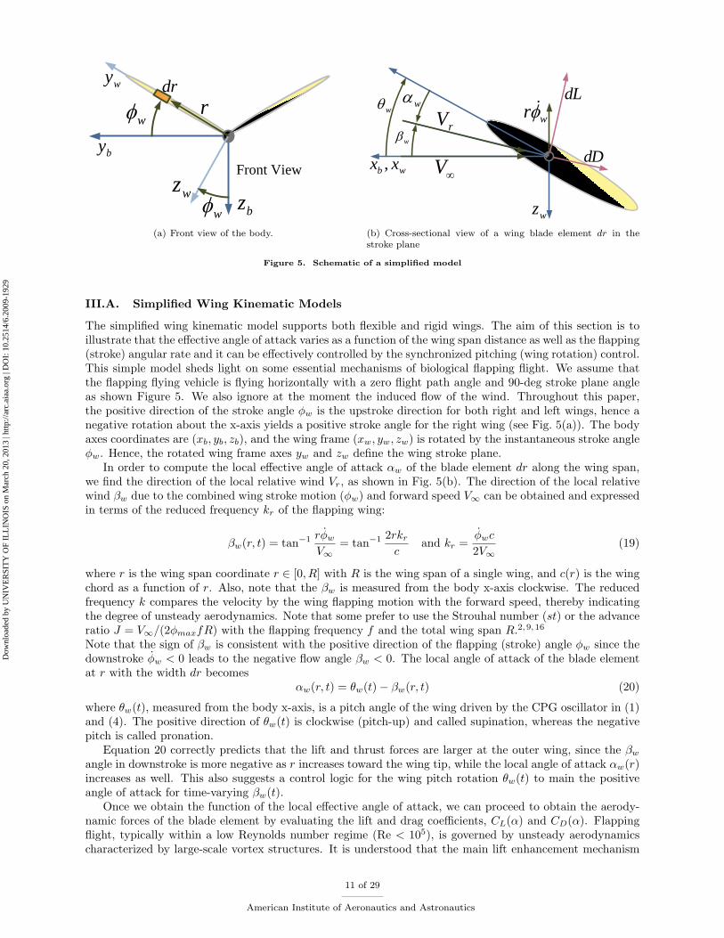
Figure 5. Schematic of a simplified model
III.A. Simplified Wing Kinematic Models
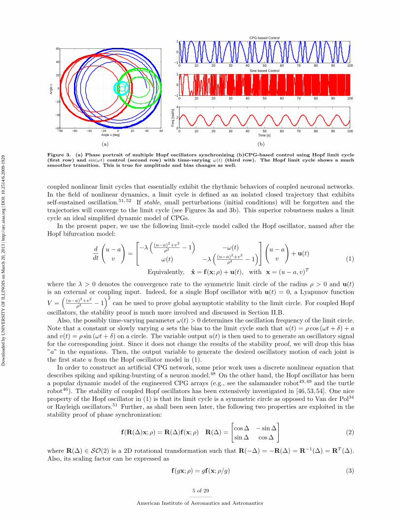
The simplified wing kinematic model supports both flexible and rigid wings. The aim of this section is toillustrate that the effective angle of attack varies as a function of the wing span distance as well as the flapping(stroke) angular rate and it can be effectively controlled by the synchronized pitching (wing rotation) control.This simple model sheds light on some essential mechanisms of biological flapping flight. We assume thatthe flapping flying vehicle is flying horizontally with a zero flight path angle and 90-deg stroke plane angleas shown Figure 5. We also ignore at the moment the induced flow of the wind. Throughout this paper,the positive direction of the stroke angle φw is the upstroke direction for both right and left wings, hence anegative rotation about the x-axis yields a positive stroke angle for the right wing (see Fig. 5(a)). The bodyaxes coordinates are (xb, yb, zb), and the wing frame (xw, yw, zw) is rotated by the instantaneous stroke angleφw. Hence, the rotated wing frame axes yw and zw define the wing stroke plane.
In order to compute the local effective angle of attack αw of the blade element dr along the wing span,we find the direction of the local relative wind Vr, as shown in Fig. 5(b). The direction of the local relativewind βw due to the combined wing stroke motion (φw) and forward speed V∞ can be obtained and expressedin terms of the reduced frequency kr of the flapping wing:
βw(r, t) = tan−1 rφwV∞
= tan−1 2rkrc
and kr =φwc
2V∞(19)
where r is the wing span coordinate r ∈ [0, R] with R is the wing span of a single wing, and c(r) is the wingchord as a function of r. Also, note that the βw is measured from the body x-axis clockwise. The reducedfrequency k compares the velocity by the wing flapping motion with the forward speed, thereby indicatingthe degree of unsteady aerodynamics. Note that some prefer to use the Strouhal number (st) or the advanceratio J = V∞/(2φmaxfR) with the flapping frequency f and the total wing span R.2,9, 16
Note that the sign of βw is consistent with the positive direction of the flapping (stroke) angle φw since thedownstroke φw < 0 leads to the negative flow angle βw < 0. The local angle of attack of the blade elementat r with the width dr becomes
αw(r, t) = θw(t)− βw(r, t) (20)
where θw(t), measured from the body x-axis, is a pitch angle of the wing driven by the CPG oscillator in (1)and (4). The positive direction of θw(t) is clockwise (pitch-up) and called supination, whereas the negativepitch is called pronation.
Equation 20 correctly predicts that the lift and thrust forces are larger at the outer wing, since the βwangle in downstroke is more negative as r increases toward the wing tip, while the local angle of attack αw(r)increases as well. This also suggests a control logic for the wing pitch rotation θw(t) to main the positiveangle of attack for time-varying βw(t).
Once we obtain the function of the local effective angle of attack, we can proceed to obtain the aerody-namic forces of the blade element by evaluating the lift and drag coefficients, CL(α) and CD(α). Flappingflight, typically within a low Reynolds number regime (Re < 105), is governed by unsteady aerodynamicscharacterized by large-scale vortex structures. It is understood that the main lift enhancement mechanism
11 of 29
American Institute of Aeronautics and Astronautics
Dow
nloa
ded
by U
NIV
ER
SIT
Y O
F IL
LIN
OIS
on
Mar
ch 2
0, 2
013
| http
://ar
c.ai
aa.o
rg |
DO
I: 1
0.25
14/6
.200
9-19
29
of flapping flight is governed by (1) the leading edge vortex (LEV) that leads to delayed stall at a very highangle of attack, (2) the rotational circulation lift, and (3) wake capture that generate aerodynamic forcesduring flapping angle reversals.6 In particular, Dickinson’s series of papers,6,9 by cross-validating the nu-merical computation and experimentation using the Robofly, shows that a quasi-steady aerodynamic modelpredicts the aerodynamic coefficients reasonably well. CFD methods that would require numerous hours anddays of computation for more accurate unsteady aerodynamics are not suited for a control design, especiallywhen such modeling errors can be addressed by robust control. Further, this quasi-steady approximationmethod can be verified and improved by the experimental set-up described in Section V.
The seminal paper by Dickison,6 used a hovering pair of wings without a forward speed as follows
CL(αw) = 0.225 + 1.58 sin(2.13αw − 7.2 deg)CD(αw) = 1.92− 1.55 cos(2.04αw − 9.82 deg)
(21)
It should be noted that Dickinson’s robotfly’s setup used a horizontal stroke plane, as typically seen in insectflight, whereas we assume a 90-deg stroke plane angle. Note that the angle αw for a general flapping wingis time-varying, as described in this section. Also, a recent paper9 that considers a nonzero-forward speed.These aerodynamic coefficients become functions of the reduced frequency (kr) with a non-zero forwardspeed:
CL(αw) = Kl1(kr) sinαw cosαw (22)
CD(αw) = Kd1(kr) sin2 αw +Kd0(kr), kr =φw,maxc
2V∞(23)
where we modified the definition of the reduced frequency kr slightly with a constant maximum strokeangular rate φw,max, since φw in (19) is time-varying. The experimental setup introduced in this paperallows us to measure such coefficients.From the quasi-steady approximation of CL and CD, we can compute the lift and drag forces acting on theblade element with the width dr as follows.
dL =12ρCL (αw(r, t)) c(r)V 2
r (r, t)dr (24)
dD =12ρCD (αw(r, t)) c(r)V 2
r (r, t)dr
where Vr(r, t) =√
(rφ)2 + V 2∞ and
In addition, Ellington10 derived the wing circulation Γr = παc2(3/4 − x0) based on the Kutta-Joukowskicondition. This quasi-steady approximation for the rotational lift can be written as
dLrot =12ρ
(2π(
34− x0)
)c2(r)Vr(r, t)αwdr (25)
where x0 is the location of the pitch axis along the mean chord length. Also, αw can be computed from (20)and often approximated reasonably well by the angular rate of the wing pitch motion θw.
The total x and z directional forces of a single wing (either right or left) in the body frame are obtainedas
Fwz =∫ R
r=0
dD sinβw − (dL+ dLrot) cosβw (26)
Fwx =∫ R
r=0
−(dL+ dLrot) sinβw − dD cosβw
Note that the positive direction of zb is downward as shown in Fig. 5.
III.B. Three-Dimensional Wing Kinematics and Aerodynamic Forces
We present a more realistic modeling that encompasses a tilted stroke angle, the lead-lag motion, and therelative body velocity, in addition to the stroke and pitch angles. In deriving these equations, the actual
12 of 29
American Institute of Aeronautics and Astronautics
Dow
nloa
ded
by U
NIV
ER
SIT
Y O
F IL
LIN
OIS
on
Mar
ch 2
0, 2
013
| http
://ar
c.ai
aa.o
rg |
DO
I: 1
0.25
14/6
.200
9-19
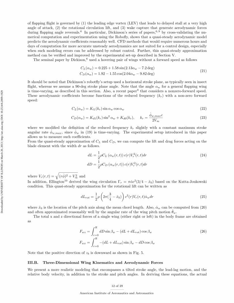
29
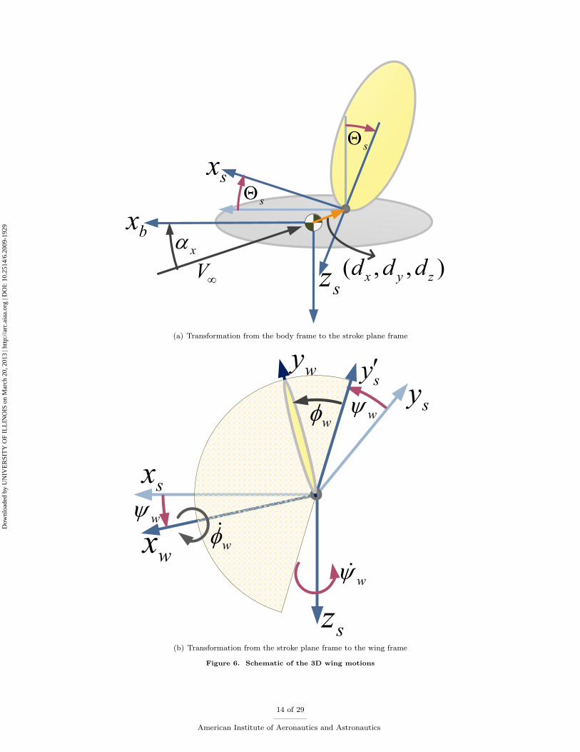
control degrees-of-freedom of the robotic bat MAV testbed, which is presented in Section V, are considered.Figure 6a shows a side view of the flapping flying MAV with the body frame xb = (xb, yb, zb)T and thestroke-plane frame xs = (xs, ys, zs)T of the right wing. In this section, we present only the equations ofthe right wing since the similar expressions for the left wing can straightforwardly follow. The center of thestroke-plane frame is located at (dx, dy, dz), and it is tilted by the inclination angle Θs(t), which can be afunction of time and the forward velocity. Without the lead-lag motion, the axes ys and zs define the strokeplane. Hence, the transformation between these coordinate axes can be given by
xb = Tbs(Θs)xs + (dx, dy, dz)T , where Tbs(Θs) =
cos Θs 0 sin Θs
0 1 0− sin Θs 0 cos Θs
(27)
where in this paper Tbs denotes the transformation from xs to xb, whereas Tsb = TTbs would correspond to
the transformation from xb to xs.For a hovering insect, the stroke plane is almost horizontal (i.e., Θs = 90 deg in our coordinate definitionin Fig 6a), resulting in forward and backward reciprocating motions. This is the assumption used for someprior work.6,9, 19,20 In contrast, the stroke angle of birds and bats varies as a function of flight speed; at alow speed, the angle is almost horizontal (Θs = 90 deg) and it approaches Θs = 0 deg as the flight speedincreases.
If there is no lead-lag motion, the additional transformation for a wing stroke angle φw, similar to Fig. 5b,would complete all the required transformation between the body frame and the wing frame. However, anonzero lead-lag angle further complicates the wing kinematics. Choosing the rotational axes for flapping,lead-lag, and pitch depends on the actual hardware setup and actuators, and our choice is influenced bythe robotic bat MAV presented in this paper. In contrast with Azuma’s derivation in [3] where the strokeangle Θs(t) is dependent on the φw(t) and the lead-lag angle ψw(t), our Θs(t) is an independent controlvariable. Our decision is based on the observation that Θs(t) can be an important control variable for efficientengineered flapping flight. Further, this kind of actuator mechanism is easier to implement and control. Asshown in Fig. 6b, the lead-lag angle is defined by the rotation about the zs axis- the z-axis in the strokeplane frame. In contrast with the fixed angle rotation in [3], then we rotate about the new x-axis to obtainthe wing frame xw. The positive direction of ψw is the forward direction, while the positive stroke angleφw indicates an upstroke motion. This sign convention does not agree with the original positive direction ofrotation for the right wing, so extra care should be taken to determine the correct angular transformationmatrices.
For the right wing, the transformation between the stroke plane frame (xs) and the wing frame (xw) canbe written as
xs = Tsw(φw, ψw)xw =
cosψw sinψw 0− sinψw cosψw 0
0 0 1
1 0 0
0 cosφw sinφw0 − sinφw cosφw
xw (28)
=
cosψw cosφw sinψw sinφw sinψw− sinψw cosφw cosψw sinw φw cosψw
0 − sinφw cosφw
xw
In order to compute the local lift and drag of a blade element, we need to transform the velocities inbody coordinates to the incident velocities in the rotated wing frame. For example, consider the free-streamforward speed V∞ with the body angle of attack αx and the side-slip angle αy. Note that αy is commonlydenoted by β in the aerospace community, but in this paper β denotes the direction of the relative wind ofa blade element. Then, the free-stream velocity in the body frame can be written as
Vb = (V∞ cosαy cosαx, V∞ sinαy, V∞ cosαy sinαx)T + vi + vE (29)
where vi and vE denote the induced velocity vector and the wind velocity vector respectively. In otherwords, in the absence of vi and vE , the vector Vb equals the velocity of the vehicle in the body frame. Letus assume that αx and αy include the effects of the induced velocity and vE is small.
Then, the free-velocity vector Vb in the body frame can be transformed to the wind frame. In addition, wecan also compute the additional velocity on the wing frame induced from the body angular rate Ωb = (p, q, r)T
13 of 29
American Institute of Aeronautics and Astronautics
Dow
nloa
ded
by U
NIV
ER
SIT
Y O
F IL
LIN
OIS
on
Mar
ch 2
0, 2
013
| http
://ar
c.ai
aa.o
rg |
DO
I: 1
0.25
14/6
.200
9-19
29
V∞
bxxα
sΘ
sΘ
( , , )x y zd d dsz
sx
9090
sz
sx
sysy′
wx
wy
wψ
wψ
wψ
wφ
wφ
(a) Transformation from the body frame to the stroke plane frame
V∞
bxxα
sΘ
sΘ
( , , )x y zd d dsz
sx
9090
sz
sx
sysy′
wx
wy
wψ
wψ
wψ
wφ
wφ
(b) Transformation from the stroke plane frame to the wing frame
Figure 6. Schematic of the 3D wing motions
14 of 29
American Institute of Aeronautics and Astronautics
Dow
nloa
ded
by U
NIV
ER
SIT
Y O
F IL
LIN
OIS
on
Mar
ch 2
0, 2
013
| http
://ar
c.ai
aa.o
rg |
DO
I: 1
0.25
14/6
.200
9-19
29
and the offset distance d = (dx, dy, dz)T of the stroke plane frame (see Fig. 6a). By adding these two terms,we can obtain
Vwb = Tws(φw, ψw)Tsb(Θs)(Vb + Ωb × d) (30)
In order to compute the rotational velocity on the wing frame produced by the flapping φw and lead-lagψw motions, as well as a relatively slower stroke angle change Θs(t), it is more convenient to construct theangular rate vector in the stroke plane frame as follows
Ωtot = Tsb(Θs)Ωb +
− cosψwφwsinψwφw + Θs
−ψw
(31)
Then, we can compute the induced rotational velocity from the wing motions of the blade element dr
Vwrot = (Tws(φw, ψw)Ωtot)×
0r
0
+
xw(r)yw(r)zw(r)
+
xw(r)yw(r)zw(r)
(32)
where xw(r), yw(r) and zw(r) are the deformation of the blade element due to aeroelastic deformation oractive cambering control that can be found in bat flight. Hence, the derivations in this section can be usedfor flexible wing models, although the CL(α) and CD(α) functions should be corrected for such camberredwing shapes.
By adding Vwb in (30) and Vw
rot in (32), we can obtain the total velocity of the wind at the blade element,distanced from r on the wing span axis, as follows
Vw =
VwxVwy
Vwz
= Tws(φw, ψw)Tsb(Θs)(Vb+Ωb×d)+(Tws(φw, ψw)Ωtot)×
0r
0
+
xw(r)yw(r)zw(r)
+
xw(r)yw(r)zw(r)
(33)
A similar expressions can be obtained for the left wing.Now, we can obtain the local effective angle of attack αw of the blade element to determine aerodynamicforces and torque. Let us assume that the deformation of a rigid wing is negligible and there is no activecambering control. Also, the contribution from the body angular rate Ωb is small. Then, (33) reduces toVwxVwy
Vwz
= Tws(φw, ψw)Tsb(Θs)Vb +
Tws(φw, ψw)
− cosψwφwsinψwφw + Θs
−ψw
×
0r
0
(34)
=
V∞ cosψw cos(Θs + αx) cosαy − V∞ sinψw sinαy − r cosψw sinφwΘs + r cosφwψwV∞ cosαy (cosφw cos (Θs + αx) sinψw − sinφw sin (Θs + αx)) + V∞ cosφw cosψw sinαy
V∞ cosαy (cos (Θs + αx) sinφw sinψw + cosφw sin (Θs + αx)) + V∞ cosψw sinφw sinαy − r(sinψwΘs + φw)
Then, similar to (19), we can obtain the local incident angle βw, the angle of attack αb, and the speed of thewind Vr on the blade element on the right wing as follows
βw(r, t) = tan−1 −VwzVwx
(35)
αw(r, t) = θw(t)− βw(r, t) (36)
V 2r (r, t) =
√V 2wx + V 2
wz (37)
where we neglected the flow along the wing span Vwy and the wing rotation θw(t) controller can be properlydesigned to yield a positive angle of attack for both upstroke and downstroke motions (see Fig. 5b).
The x and z directional forces Fwx and Fwz on the wing frame given in (26), computed with dL, dDin(24) and dLrot in (25), can be transformed into the forces in the vehicle body frame:
Fright =
FxFyFz
right
= Tbs(Θs)Tsw(φw, ψw)
Fwx0Fwz
right
(38)
15 of 29
American Institute of Aeronautics and Astronautics
Dow
nloa
ded
by U
NIV
ER
SIT
Y O
F IL
LIN
OIS
on
Mar
ch 2
0, 2
013
| http
://ar
c.ai
aa.o
rg |
DO
I: 1
0.25
14/6
.200
9-19
29
where we added the subscript right to indicate that this force vector is from the right wing. A similarexpression can be obtained for the left wing (Fleft). Note that each wing has different wing angular parameterssuch as φw, ψw, and θw, although the stroke plane angle Θs is the same for both wings. In symmetric wingmotions, the Fy forces from both wings cancel each other.
In order to compute the rotational moments generated by the aerodynamic forces, we first calculate theposition of the wing blade element with respect to the body frame
p(r) = Tbs(Θs)Tsw(φw, ψw)
0r
0
+
dxdydz
(39)
where dx and dz indicate the origin of the stroke plane frame in the body frame.Then, we can compute the aerodynamic moments with respect to the c.g.dMx
dMy
dMz
= p(r)×
Tbs(Θs)Tsw(φw, ψw)
−(dL+ dLrot) sinβw − dD cosβw0
dD sinβw − (dL+ dLrot) cosβw
+
dMx0
dMy0
dMz0
(40)
dMx0
dMy0
dMz0
= Tbs(Θs)Tsw(φw, ψw)Tθw(θw)
12ρV 2
r c(r)dr
rcl0
c(r)(cm0 + cα,wαw)rcn0
(41)
Mx =∫ R
r=0
dMx, My =∫ R
r=0
dMy, Mz =∫ R
r=0
dMz (42)
where dMx0, dMx0, and dMx0 denote the constant aerodynamic moments that include the moment at themean aerodynamic center, computed by the moment coefficients cl0, cm0, cα,w, and cn0. Also, R is the wingspan. The additional transformation Tθw
(θw) rotates the wing frame about the yw axis by the wing pitchrotation angle θw.
III.C. Dynamic Modeling
By combining all the forces and moments from the right wing and the left wing, we can derive 6-DOFequations of motion for the flapping flying MAV in the body frame, whose orientation with respect to theinertial frame is described by the Euler angles. We assume the moment of inertia of the wing compared tothe body weight is negligible. Then, we can obtain the following set of equations. The translational motionof the c.g. of the flapping flying vehicle driven by the aerodynamic force terms in (38) can be expressed as
mVb +mΩb × Vb = Tbe(φb, θb, ψb)Fg + Fright + Fleft + A (43)
where Vb = (Vbx, Vby, Vbz)T denotes the vehicle velocity vector in the body frame, Ωb = (p, q, r)T is the bodyangular rate, and the Euler angular transformation matrix determines the orientation of the body frame withrespect to the inertial frame
Tbe(φb, θb, ψb) =
cos θb cosψb cos θb sinψb − sin θbsinφb sin θb cosψb − cosφb sinψb sinφb sin θb sinψb + cosφb cosψb sinφb cos θbcosφb sin θb cosψb + sinφb sinψb cosφb sin θb sinψb − sinφb cosψb cosφb cos θb
.
In addition, Fg = (0, 0,mg)T is the gravitational force vector in the inertial frame, while Fleft and Fright
denote the aerodynamic forces from each wing, obtained from (38). Note that each wing has different wingangular parameters such as φw, ψw, and θw, although the stroke plane angle Θs is the same for each wing.The force vector A = (Ax, Ay, Az)T represents the additional forces generated by the body (fuselage) andthe tail.
The equations of rotational motion are driven by the aerodynamic moments Mright and Mleft of eachwing that can be obtained from (40)
IbΩb + Ωb × (IbΩb) = Mright + Mleft + B (44)
where Ib is a 3 × 3 inertia matrix and the additional torque vector B = (Bx, By, Bz)T represents theaerodynamic moment from the body and the tail. The relationship between the body angular rate Ωb =
16 of 29
American Institute of Aeronautics and Astronautics
Dow
nloa
ded
by U
NIV
ER
SIT
Y O
F IL
LIN
OIS
on
Mar
ch 2
0, 2
013
| http
://ar
c.ai
aa.o
rg |
DO
I: 1
0.25
14/6
.200
9-19
29
(p, q, r)T and the Euler angle vector qb = (φb, θb, ψb)T can be determined byφbθbψb
= Z(qb)Ωb =
1 sinφb tan θb cosφb tan θb0 cosφb − sinφb0 sinφb sec θb cosφb sec θb
pqr
(45)
Note that any other orientation representations such as quaternions can be used in lieu of the Euler anglesin the preceding equations. Also, any disturbance force and torque can be added to the equations.
IV. CPG-based Flapping Flight Control and Simulation Results
The aim of this section is to show that CPG-based flight control can stabilize and control flappingflight dynamics given in Section III.C by using the synchronized and symmetry-breaking (phase difference)oscillatory motions of two main wings. In particular, we show that the dynamics can be effectively controlledwithout using aerodynamic control surfaces such as ailerons, elevators, rudders, and directional control oftail wings.
The example presented in this paper is alternating two different flight modes of flapping and glidingflight. We maintain a particular interval of altitude level, bracketing steady level flight. Longitudinal andlateral motions are nearly uncoupled, so we consider only longitudinal motion for brevity. Lateral forces aretherefore considered symmetric. Additionally, we do not consider the aerodynamics of the second joint andinstead assume each wing to be one rigid piece. That is, in (33), we set(
xw(r), yw(r), zw(r))T
= 0. (46)
This restricted kinematic and dynamic model is constructed in Simulink, allowing us to demonstrate howsimple longitudinal stability can be obtained for flapping flight driven by a CPG network. From biologicalinvestigation, Thomas and Taylor66 suggest that many birds utilize the ability to twist their wings in orderto provide a wash-out and backward-sweep combination or a wash-in and forward-sweep combination forgliding stability. This configuration can provide inherent tailless longitudinal stability. Alternatively, theysuggest that birds dynamically alter the wing sweep in order to obtain longitudinal stability in gliding flight.Our experimental apparatus is untwisted, so we choose the second method for stability in our simulations.
Gliding Mode: We assume that in gliding flight there is no reciprocal flapping motion, obviously.Therefore, we set the parameter ω(t) in the Hopf oscillator to zero. In addition, we set the coupling gainsbetween CPGs to zero. This provides us simple control of our wing by exploiting the bifurcation in Hopfoscillators, causing them to snap to a single value corresponding to the bias. We further assume that weare able to select an optimum wing angle of attack with regard to the wing size and aerodynamics, vehicleweight and velocity to maximize the glide path angle. We can then control the lead lag motion (ψw) andflapping angle (φw) by their bias parameters. With zero ω(t), these parameters should tend to their biasvalues in a non-oscillatory manner. A negative (positive) flapping angle or negative (positive) lead-lag anglecan provide a pitch-down (pitch-up) moment due to drag or lift, respectively. We have therefore reducedcontrol dimensionality to three actively controlled parameters: wing pitch, wing flapping angle, and lead-lagangle. In fact, depending on the physical characteristics of the specific vehicle, controlling only one of wingflapping angle or lead-lag angle could be sufficient for gliding stability.
Flapping Flight Control by Flapping Frequency: Seemingly more difficult than stability in glidingflight is stability in flapping flight. We propose a novel control law unique to our CPG set-up which reducescontrol dimensionality to only two parameters. The first parameter is the oscillation frequency ω(t) of thecoupled Hopf oscillators in (6). By inspecting the definitions of the local angle of attack of the wing bladeelement αw given in (20) and (35), we can find that ω(t) correlates with flapping frequency, which in turncorrelates with increased lift and thrust. Those in turn, correlate with forward (Vbx) and vertical (Vbz)velocity of the body, all other factors being equal. We can very simply control ω with the old adage, “If youwant to go faster, press the pedal further.” For example, we can consider the following control law
ω = K
∫ t
0
ωdt = K
∫ t
0
(Vx,desired − Vx,actual) dt (47)
17 of 29
American Institute of Aeronautics and Astronautics
Dow
nloa
ded
by U
NIV
ER
SIT
Y O
F IL
LIN
OIS
on
Mar
ch 2
0, 2
013
| http
://ar
c.ai
aa.o
rg |
DO
I: 1
0.25
14/6
.200
9-19
29
We can use the following corollary to show that the time-varying ω(t) does not alter the synchronizationproof of the oscillators.
Corollary 1 From the dynamic equation of the Hopf oscillator in (1), the time-varying ω(t) does not affectthe stability proof for Theorem 2
Proof 3 Since the symmetric part of f cancels the ω term and ω does not change the maximum eigenvalueof VT [f ] V. The rest of the proof follows Theorem 2.
Control of ω takes care of translational forces, but we have not yet considered rotational moments. Itshould be noted that the control of the maximum flapping stroke angle φwmax
, e.g., ρ1 = ρ5 for the CPGconfiguration in Fig. 4a, can be also used to induce similar translational control effects.
Flapping Flight Control by Phase Differences: Our second control parameter is the phase differ-ence between the lead-lag CPG and the pitching CPG ∆31 −∆21 in Figure 4a. or simply ∆32. Note thatwhen we do take the second joint into account for the dynamic modeling, we can add an additional perfor-mance parameter for the phase difference between lead-lag angle (ψw) and the second joints (φw2), with anaccompanying change in the phase difference between the first and second joints to retain flow invariance.Effectively, all phase differences can be altered as long as flow invariance is retained. Different graph config-urations may be required to obtain favorable characteristics for high-agility maneuvers and Theorem 2 canbe used to derive the exponentially and globally stabilizing gains. Additionally, our oscillator stability proofin Theorem 2 assumes constant or relatively slowly varying phase differences. However, the error terms fromthe additional time-varying parameters other than ω(t) can be obtained by the robust contraction analysis,60
which shows the boundedness of the synchronization error.
Corollary 2 For time-varying phase differences ∆ij, the synchronization of the rotated Hopf states zglobally converges to the bounded error defined by VTTT−1z.
Proof 4 Recall the relationship between the original Hopf variables x and z = T(∆ij , ρi)x in (10).Since the function T(∆ij , ρi) is nonzero, (14) becomes
z+ TT−1z = T [f(x; ρ)]− kLz (48)
Consequently, the virtual system in (18) becomes
y = VT[f(Vy + 11T /nz; ρ1)
]− kVTLVy + ε(t) (49)
where the error term ε(t) comes from the nonzero time-derivative of the T matrix since some ∆ij is time-varying.
ε(t) = −VTTT−1z (50)
Hence, although the y system in (49) is contracting, the Hopf oscillators do not perfectly synchronize becausey = 0 is no longer the particular solution. By robust contraction analysis,60 where P1(t) defines representsa desired system trajectory and P2(t)the actual system trajectory in a disturbed flow field given in (18 withthe error term. Also, consider the distance R(t) between two trajectories P1(t) and P1(t) such that
R(t) + `R(t) ≤ ‖ε(t)‖ (51)
where ` > 0 is the contraction rate of the virtual system (49) such that ` = kλmin(VT (L + LT )/2V)) − λ.Hence, the synchronization error converges to the ball of the radius ‖ε(t)‖ /`
To simply characterize the effectiveness of altering the phase difference between flapping and lead-lag,consider the largest force values over the length of a stroke. These are likely to be obtained from lift in themiddle of a downstroke. With a zero bias lead-lag and a center of gravity coinciding with the stroke plane,a phase difference of 270 between the flapping CPG and the lead-lag CPG gives Azuma’s3 elliptical modelof flapping: negative lead-lag on downstroke, positive lead-lag on upstroke. The simplest analysis combinesa maximum force with the most-negative lead-lag at the middle of the downstroke to predict a large pitch-down moment on the body. Alternatively, if we set the phase difference to 180, we see the maximum forcecoinciding with the maximum positive lead-lag at the middle of the downstroke, predicting a large pitch-up
18 of 29
American Institute of Aeronautics and Astronautics
Dow
nloa
ded
by U
NIV
ER
SIT
Y O
F IL
LIN
OIS
on
Mar
ch 2
0, 2
013
| http
://ar
c.ai
aa.o
rg |
DO
I: 1
0.25
14/6
.200
9-19
29
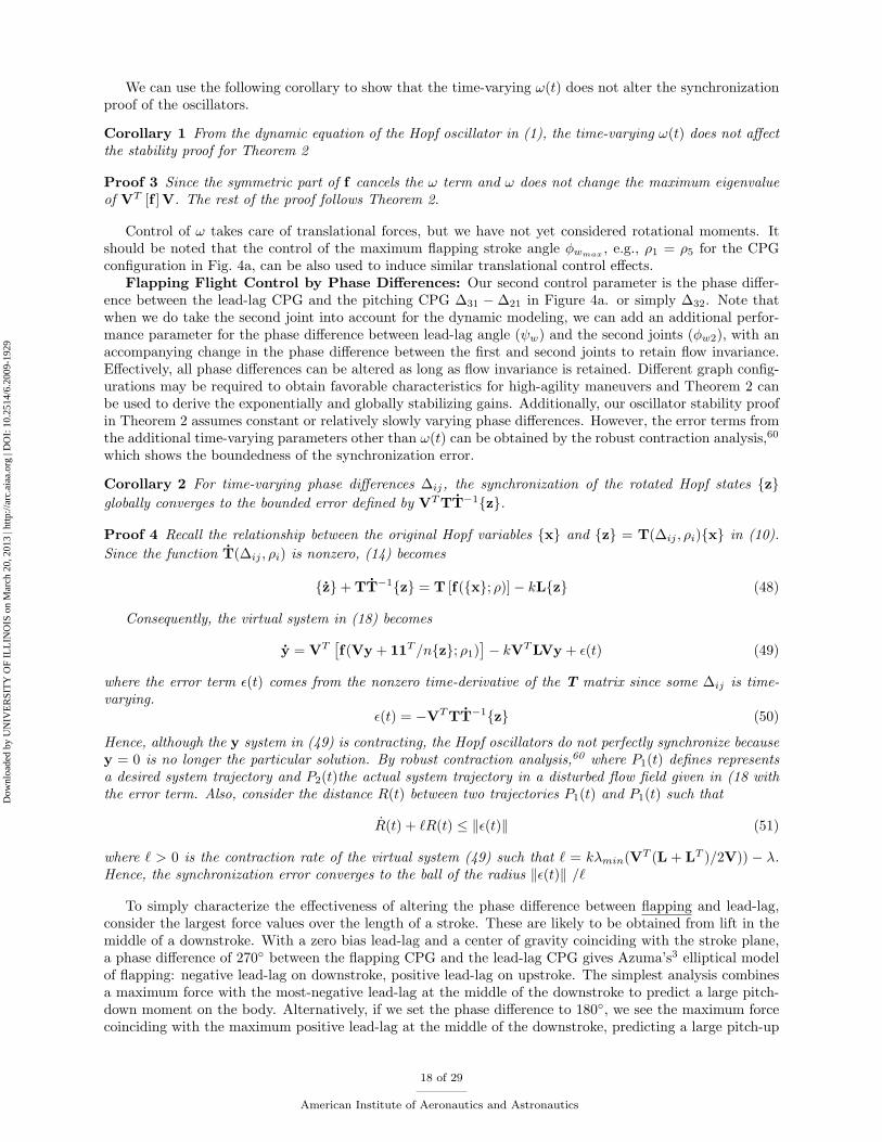
moment. We use this as our primary control variable for longitudinal stability. For the following figures, wefix ∆21 = 90. We tune our range to
θbody : [−2, 2]→ ∆31 : [180, 270] (52)
by∆31 −∆21 = −45θbody + 135 −Kθbody. (53)
0 0.5 1 1.5 2 2.5 3 3.5 4 4.5 5
−5
0
5
10
Vel
ocity
(V
e) [m
/s]
0 0.5 1 1.5 2 2.5 3 3.5 4 4.5 5−0.1
0
0.1
0.2
Bod
y an
gula
r ra
te [r
ad/s
]
0 0.5 1 1.5 2 2.5 3 3.5 4 4.5 5
−3
−2
−1
0
Time [s]
Eul
er a
ngle
[deg
]
Figure 7. State vectors of the two alternating flight modes, flapping and gliding.
0 0.5 1 1.5 2 2.5 3 3.5 4 4.5 5
−40
−20
0
20
40
Fla
ppin
g an
d Le
ad−
lag
[deg
]
Time [s]
0 0.2 0.4 0.6 0.8 1 1.2 1.4 1.6 1.8
−40
−20
0
20
40
Fla
ppin
g an
d Le
ad−
lag
(zoo
med
) [d
eg]
Time [s]
Figure 8. Flapping (φw) and lead-lag angles (ψw) of the two alternating flight modes, flapping and gliding.
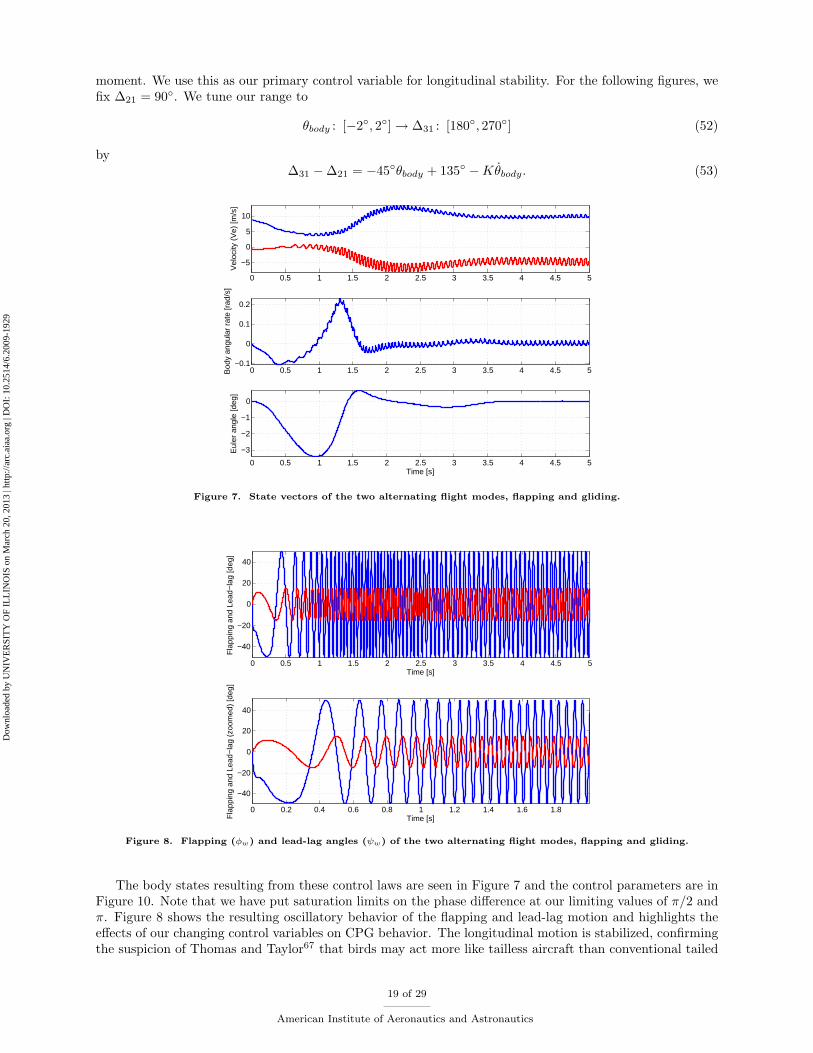
The body states resulting from these control laws are seen in Figure 7 and the control parameters are inFigure 10. Note that we have put saturation limits on the phase difference at our limiting values of π/2 andπ. Figure 8 shows the resulting oscillatory behavior of the flapping and lead-lag motion and highlights theeffects of our changing control variables on CPG behavior. The longitudinal motion is stabilized, confirmingthe suspicion of Thomas and Taylor67 that birds may act more like tailless aircraft than conventional tailed
19 of 29
American Institute of Aeronautics and Astronautics
Dow
nloa
ded
by U
NIV
ER
SIT
Y O
F IL
LIN
OIS
on
Mar
ch 2
0, 2
013
| http
://ar
c.ai
aa.o
rg |
DO
I: 1
0.25
14/6
.200
9-19
29
0 1 2 3 4 5 6 7 8 9 10
−8
−6
−4
−2
0
2
4
6
8
10
12
Vel
ocity
Ve
[m/s
]
time [s]
Figure 9. Velocity vector of the two alternating flight modes, flapping and gliding.
0 0.5 1 1.5 2 2.5 3 3.5 4 4.5 5
5
10
15
20
Time [s]
Ω [r
ad/s
]
0 0.5 1 1.5 2 2.5 3 3.5 4 4.5 51.6
1.8
2
2.2
2.4
2.6
2.8
3
Time [s]
Pha
se D
iffer
ence
∆32
[rad
]
Figure 10. Control inputs of the two alternating flight modes, flapping and gliding.
20 of 29
American Institute of Aeronautics and Astronautics
Dow
nloa
ded
by U
NIV
ER
SIT
Y O
F IL
LIN
OIS
on
Mar
ch 2
0, 2
013
| http
://ar
c.ai
aa.o
rg |
DO
I: 1
0.25
14/6
.200
9-19
29
aircraft. This model has no stabilizing tail-induced moment and therefore sheds light on the fact that manybirds can fly without their tail. Including a constant or angle of attack dependent body/tail moment willonly serve to alter the equilibrium point. Altering the range through which we control the phase differenceallows us to tune the equilibrium point as we desire for any body/tail behavior.
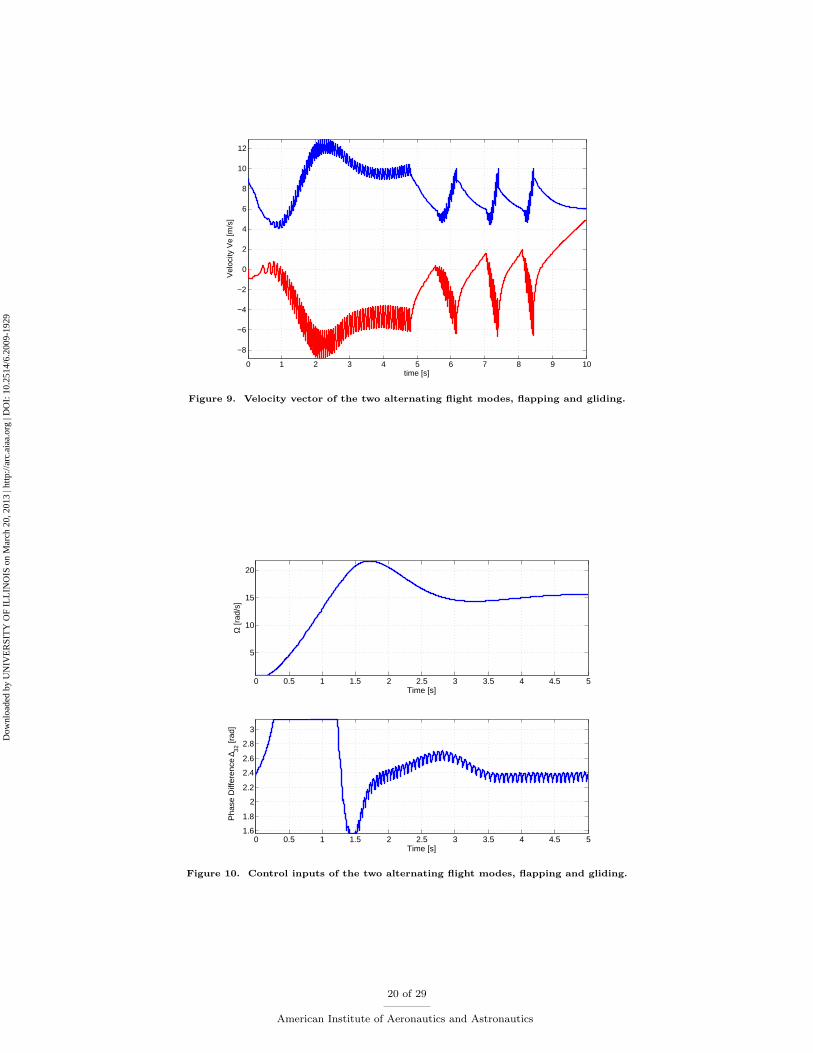
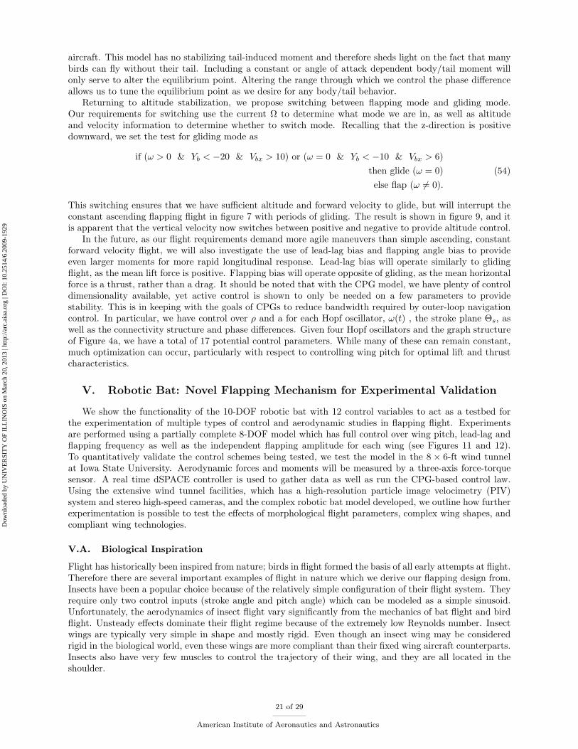
Returning to altitude stabilization, we propose switching between flapping mode and gliding mode.Our requirements for switching use the current Ω to determine what mode we are in, as well as altitudeand velocity information to determine whether to switch mode. Recalling that the z-direction is positivedownward, we set the test for gliding mode as
if (ω > 0 & Yb < −20 & Vbx > 10) or (ω = 0 & Yb < −10 & Vbx > 6)then glide (ω = 0)else flap (ω 6= 0).
(54)
This switching ensures that we have sufficient altitude and forward velocity to glide, but will interrupt theconstant ascending flapping flight in figure 7 with periods of gliding. The result is shown in figure 9, and itis apparent that the vertical velocity now switches between positive and negative to provide altitude control.
In the future, as our flight requirements demand more agile maneuvers than simple ascending, constantforward velocity flight, we will also investigate the use of lead-lag bias and flapping angle bias to provideeven larger moments for more rapid longitudinal response. Lead-lag bias will operate similarly to glidingflight, as the mean lift force is positive. Flapping bias will operate opposite of gliding, as the mean horizontalforce is a thrust, rather than a drag. It should be noted that with the CPG model, we have plenty of controldimensionality available, yet active control is shown to only be needed on a few parameters to providestability. This is in keeping with the goals of CPGs to reduce bandwidth required by outer-loop navigationcontrol. In particular, we have control over ρ and a for each Hopf oscillator, ω(t) , the stroke plane Θs, aswell as the connectivity structure and phase differences. Given four Hopf oscillators and the graph structureof Figure 4a, we have a total of 17 potential control parameters. While many of these can remain constant,much optimization can occur, particularly with respect to controlling wing pitch for optimal lift and thrustcharacteristics.
V. Robotic Bat: Novel Flapping Mechanism for Experimental Validation
We show the functionality of the 10-DOF robotic bat with 12 control variables to act as a testbed forthe experimentation of multiple types of control and aerodynamic studies in flapping flight. Experimentsare performed using a partially complete 8-DOF model which has full control over wing pitch, lead-lag andflapping frequency as well as the independent flapping amplitude for each wing (see Figures 11 and 12).To quantitatively validate the control schemes being tested, we test the model in the 8 × 6-ft wind tunnelat Iowa State University. Aerodynamic forces and moments will be measured by a three-axis force-torquesensor. A real time dSPACE controller is used to gather data as well as run the CPG-based control law.Using the extensive wind tunnel facilities, which has a high-resolution particle image velocimetry (PIV)system and stereo high-speed cameras, and the complex robotic bat model developed, we outline how furtherexperimentation is possible to test the effects of morphological flight parameters, complex wing shapes, andcompliant wing technologies.
V.A. Biological Inspiration
Flight has historically been inspired from nature; birds in flight formed the basis of all early attempts at flight.Therefore there are several important examples of flight in nature which we derive our flapping design from.Insects have been a popular choice because of the relatively simple configuration of their flight system. Theyrequire only two control inputs (stroke angle and pitch angle) which can be modeled as a simple sinusoid.Unfortunately, the aerodynamics of insect flight vary significantly from the mechanics of bat flight and birdflight. Unsteady effects dominate their flight regime because of the extremely low Reynolds number. Insectwings are typically very simple in shape and mostly rigid. Even though an insect wing may be consideredrigid in the biological world, even these wings are more compliant than their fixed wing aircraft counterparts.Insects also have very few muscles to control the trajectory of their wing, and they are all located in theshoulder.
21 of 29
American Institute of Aeronautics and Astronautics
Dow
nloa
ded
by U
NIV
ER
SIT
Y O
F IL
LIN
OIS
on
Mar
ch 2
0, 2
013
| http
://ar
c.ai
aa.o
rg |
DO
I: 1
0.25
14/6
.200
9-19
29
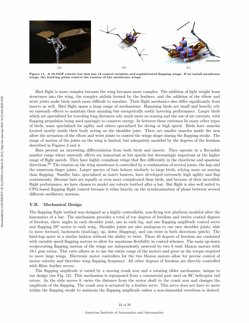
(a) (b) (c)
Figure 11. A 10-DOF robotic bat that has 12 control variables and sophisticated flapping wings. If we install membranewings, the hind-leg joints control the tension of the membrane wings.
Bird flight is more complex because the wing becomes more complex. The addition of light weight bonestructures into the wing, the complex airfoils formed by the feathers, and the addition of the elbow andwrist joints make birds much more difficult to simulate. Their flight mechanics also differ significantly frominsects as well. Bird flight spans a large range of mechanisms. Humming birds are small and heavily relyon unsteady effects to maintain their amazing but energetically costly hovering performance. Larger birdswhich are specialized for traveling long distances rely much more on soaring and the use of air currents, withflapping propulsion being used sparingly to conserve energy. In between these extremes lie many other typesof birds, some specialized for agility and others specialized for diving or high speed. Birds have muscleslocated mostly inside their body acting on the shoulder joint. There are smaller muscles inside the armallow the actuation of the elbow and wrist joints to control the wings shape during the flapping stroke. Therange of motion of the joints on the wing is limited, but adequately modeled by the degrees of the freedomdescribed in Figures 2 and 4.
Bats present an interesting differentiation from both birds and insects. They operate in a Reynoldsnumber range where unsteady effects are important at low speeds but decreasingly important at the higherrange of flight speeds. They have highly compliant wings that flex differently in the chordwise and spanwisedirections.68 The tension on the wing membrane is controlled by a combination of several joints, the legs andthe numerous finger joints. Larger species of bats behave similarly to large birds, relying more on soaringthan flapping. Smaller bats, specialized as insect hunters, have developed extremely high agility and flapcontinuously. Because bats are equally or even more complicated than birds, and because of their incredibleflight performance, we have chosen to model our robotic testbed after a bat. Bat flight is also well suited toCPG-based flapping flight control because it relies heavily on the synchronization of phase between severaldifferent oscillatory motions.
V.B. Mechanical Design
The flapping flight testbed was designed as a highly controllable, non-flying test platform modeled after thekinematics of a bat. The mechanism provides a total of ten degrees of freedom and twelve control degreesof freedom, three angles in each shoulder joint, one in each leg, and one flapping amplitude control servoand flapping DC motor in each wing. Shoulder joints are also analogous to our own shoulder joints, ableto move forward, backwards (lead-lag), up, down (flapping), and can twist in both directions (pitch). Thehind-legs move in a similar fashion without the ability to twist. These 10 degrees of freedom are combinedwith variable speed flapping motors to allow for maximum flexibility in control schemes. The main up-downreciprocating flapping motion of the wings are independently powered by two 8 watt Maxon motors with19:1 gear ratios. This ratio allows us to use the entire range of the motors and gives us the torque requiredto move large wings. Electronic motor controllers for the two Maxon motors allow for precise control ofmotor velocity and therefore wing flapping frequency. All other degrees of freedom are directly controlledwith Hitec feather servos.
The flapping amplitude is varied by a moving crank arm and a rotating slider mechanism, unique toour design (see Fig. 12). This mechanism is repurposed from a commercial part used on RC helicopter tailrotors. As the slide moves it varies the distance from the motor shaft to the crank arm and changes theamplitude of the flapping. The crank arm is actuated by a feather servo. This servo does not have to movewithin the flapping stroke to maintain the flapping amplitude unless a non-sinusoidal waveform is desired.
22 of 29
American Institute of Aeronautics and Astronautics
Dow
nloa
ded
by U
NIV
ER
SIT
Y O
F IL
LIN
OIS
on
Mar
ch 2
0, 2
013
| http
://ar
c.ai
aa.o
rg |
DO
I: 1
0.25
14/6
.200
9-19
29
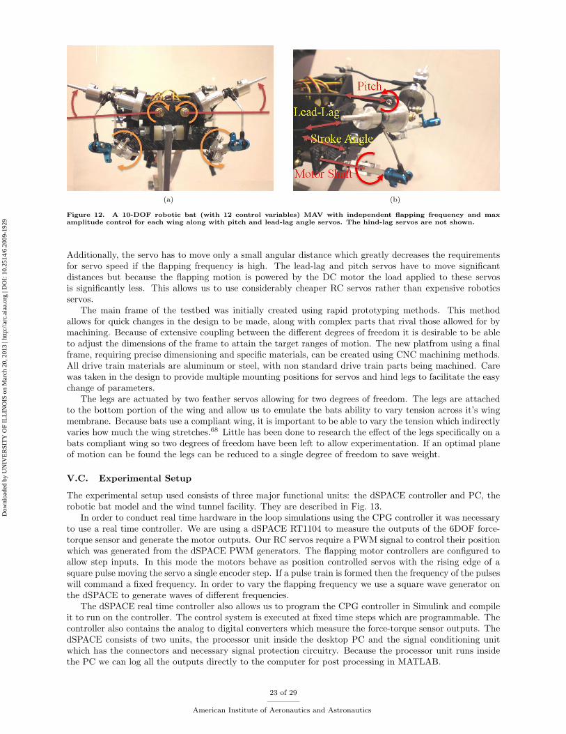
(a) (b)
Figure 12. A 10-DOF robotic bat (with 12 control variables) MAV with independent flapping frequency and maxamplitude control for each wing along with pitch and lead-lag angle servos. The hind-lag servos are not shown.
Additionally, the servo has to move only a small angular distance which greatly decreases the requirementsfor servo speed if the flapping frequency is high. The lead-lag and pitch servos have to move significantdistances but because the flapping motion is powered by the DC motor the load applied to these servosis significantly less. This allows us to use considerably cheaper RC servos rather than expensive roboticsservos.
The main frame of the testbed was initially created using rapid prototyping methods. This methodallows for quick changes in the design to be made, along with complex parts that rival those allowed for bymachining. Because of extensive coupling between the different degrees of freedom it is desirable to be ableto adjust the dimensions of the frame to attain the target ranges of motion. The new platfrom using a finalframe, requiring precise dimensioning and specific materials, can be created using CNC machining methods.All drive train materials are aluminum or steel, with non standard drive train parts being machined. Carewas taken in the design to provide multiple mounting positions for servos and hind legs to facilitate the easychange of parameters.
The legs are actuated by two feather servos allowing for two degrees of freedom. The legs are attachedto the bottom portion of the wing and allow us to emulate the bats ability to vary tension across it’s wingmembrane. Because bats use a compliant wing, it is important to be able to vary the tension which indirectlyvaries how much the wing stretches.68 Little has been done to research the effect of the legs specifically on abats compliant wing so two degrees of freedom have been left to allow experimentation. If an optimal planeof motion can be found the legs can be reduced to a single degree of freedom to save weight.
V.C. Experimental Setup
The experimental setup used consists of three major functional units: the dSPACE controller and PC, therobotic bat model and the wind tunnel facility. They are described in Fig. 13.
In order to conduct real time hardware in the loop simulations using the CPG controller it was necessaryto use a real time controller. We are using a dSPACE RT1104 to measure the outputs of the 6DOF force-torque sensor and generate the motor outputs. Our RC servos require a PWM signal to control their positionwhich was generated from the dSPACE PWM generators. The flapping motor controllers are configured toallow step inputs. In this mode the motors behave as position controlled servos with the rising edge of asquare pulse moving the servo a single encoder step. If a pulse train is formed then the frequency of the pulseswill command a fixed frequency. In order to vary the flapping frequency we use a square wave generator onthe dSPACE to generate waves of different frequencies.
The dSPACE real time controller also allows us to program the CPG controller in Simulink and compileit to run on the controller. The control system is executed at fixed time steps which are programmable. Thecontroller also contains the analog to digital converters which measure the force-torque sensor outputs. ThedSPACE consists of two units, the processor unit inside the desktop PC and the signal conditioning unitwhich has the connectors and necessary signal protection circuitry. Because the processor unit runs insidethe PC we can log all the outputs directly to the computer for post processing in MATLAB.
23 of 29
American Institute of Aeronautics and Astronautics
Dow
nloa
ded
by U
NIV
ER
SIT
Y O
F IL
LIN
OIS
on
Mar
ch 2
0, 2
013
| http
://ar
c.ai
aa.o
rg |
DO
I: 1
0.25
14/6
.200
9-19
29
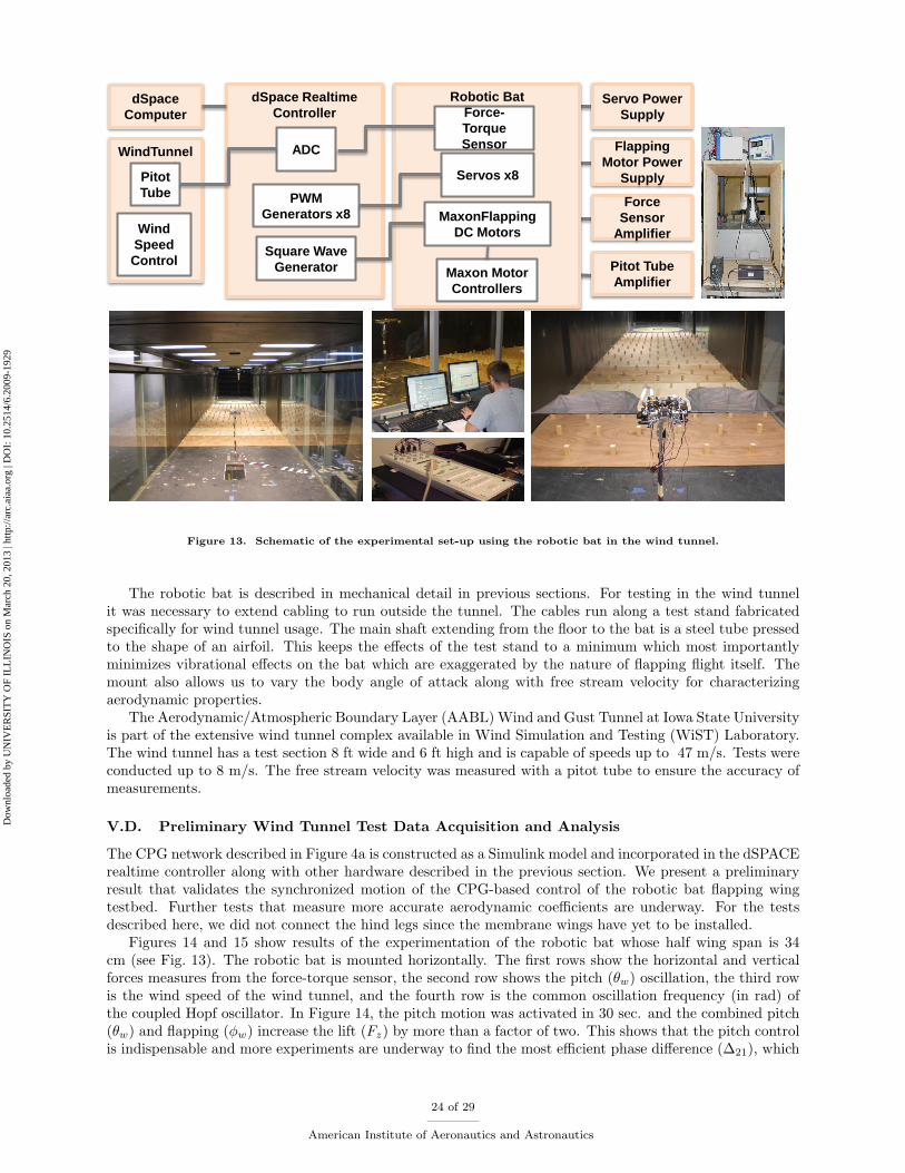
dSpace
Computer
dSpace Realtime
Controller
ADC
PWM
Generators x8
Square Wave
Generator
Robotic Bat
Force-
Torque
Sensor
MaxonFlapping
DC Motors
Servos x8
Maxon Motor
Controllers
Flapping
Motor Power
Supply
Pitot Tube
Amplifier
Force
Sensor
Amplifier
Servo Power
Supply
WindTunnel
Tunnel
Wind
Speed
Control
Pitot
Tube
Figure 13. Schematic of the experimental set-up using the robotic bat in the wind tunnel.
The robotic bat is described in mechanical detail in previous sections. For testing in the wind tunnelit was necessary to extend cabling to run outside the tunnel. The cables run along a test stand fabricatedspecifically for wind tunnel usage. The main shaft extending from the floor to the bat is a steel tube pressedto the shape of an airfoil. This keeps the effects of the test stand to a minimum which most importantlyminimizes vibrational effects on the bat which are exaggerated by the nature of flapping flight itself. Themount also allows us to vary the body angle of attack along with free stream velocity for characterizingaerodynamic properties.
The Aerodynamic/Atmospheric Boundary Layer (AABL) Wind and Gust Tunnel at Iowa State Universityis part of the extensive wind tunnel complex available in Wind Simulation and Testing (WiST) Laboratory.The wind tunnel has a test section 8 ft wide and 6 ft high and is capable of speeds up to 47 m/s. Tests wereconducted up to 8 m/s. The free stream velocity was measured with a pitot tube to ensure the accuracy ofmeasurements.
V.D. Preliminary Wind Tunnel Test Data Acquisition and Analysis
The CPG network described in Figure 4a is constructed as a Simulink model and incorporated in the dSPACErealtime controller along with other hardware described in the previous section. We present a preliminaryresult that validates the synchronized motion of the CPG-based control of the robotic bat flapping wingtestbed. Further tests that measure more accurate aerodynamic coefficients are underway. For the testsdescribed here, we did not connect the hind legs since the membrane wings have yet to be installed.
Figures 14 and 15 show results of the experimentation of the robotic bat whose half wing span is 34cm (see Fig. 13). The robotic bat is mounted horizontally. The first rows show the horizontal and verticalforces measures from the force-torque sensor, the second row shows the pitch (θw) oscillation, the third rowis the wind speed of the wind tunnel, and the fourth row is the common oscillation frequency (in rad) ofthe coupled Hopf oscillator. In Figure 14, the pitch motion was activated in 30 sec. and the combined pitch(θw) and flapping (φw) increase the lift (Fz) by more than a factor of two. This shows that the pitch controlis indispensable and more experiments are underway to find the most efficient phase difference (∆21), which
24 of 29
American Institute of Aeronautics and Astronautics
Dow
nloa
ded
by U
NIV
ER
SIT
Y O
F IL
LIN
OIS
on
Mar
ch 2
0, 2
013
| http
://ar
c.ai
aa.o
rg |
DO
I: 1
0.25
14/6
.200
9-19
29
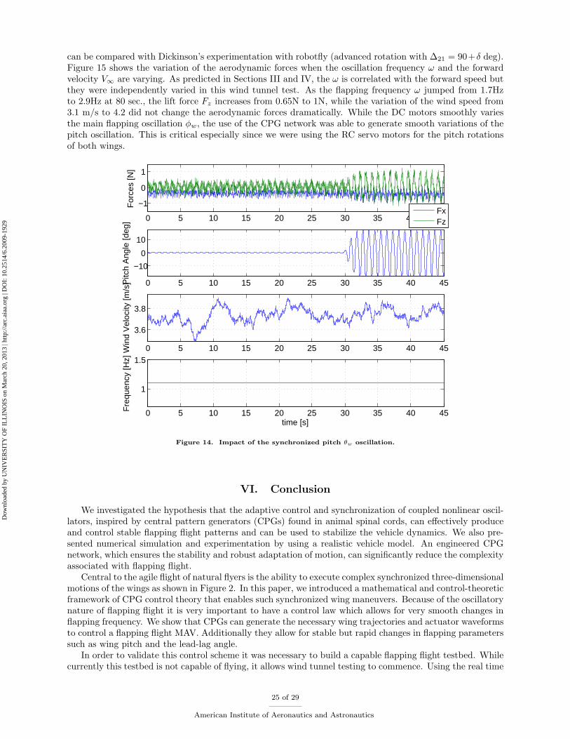
can be compared with Dickinson’s experimentation with robotfly (advanced rotation with ∆21 = 90+δ deg).Figure 15 shows the variation of the aerodynamic forces when the oscillation frequency ω and the forwardvelocity V∞ are varying. As predicted in Sections III and IV, the ω is correlated with the forward speed butthey were independently varied in this wind tunnel test. As the flapping frequency ω jumped from 1.7Hzto 2.9Hz at 80 sec., the lift force Fz increases from 0.65N to 1N, while the variation of the wind speed from3.1 m/s to 4.2 did not change the aerodynamic forces dramatically. While the DC motors smoothly variesthe main flapping oscillation φw, the use of the CPG network was able to generate smooth variations of thepitch oscillation. This is critical especially since we were using the RC servo motors for the pitch rotationsof both wings.
0 5 10 15 20 25 30 35 40 45
−1
0
1
For
ces
[N]
FxFz
0 5 10 15 20 25 30 35 40 45
−10
0
10
Pitc
h A
ngle
[deg
]
0 5 10 15 20 25 30 35 40 45
3.6
3.8
Win
d V
eloc
ity [m
/s]
0 5 10 15 20 25 30 35 40 45
1
1.5
time [s]
Fre
quen
cy [H
z]
Figure 14. Impact of the synchronized pitch θw oscillation.
VI. Conclusion
We investigated the hypothesis that the adaptive control and synchronization of coupled nonlinear oscil-lators, inspired by central pattern generators (CPGs) found in animal spinal cords, can effectively produceand control stable flapping flight patterns and can be used to stabilize the vehicle dynamics. We also pre-sented numerical simulation and experimentation by using a realistic vehicle model. An engineered CPGnetwork, which ensures the stability and robust adaptation of motion, can significantly reduce the complexityassociated with flapping flight.
Central to the agile flight of natural flyers is the ability to execute complex synchronized three-dimensionalmotions of the wings as shown in Figure 2. In this paper, we introduced a mathematical and control-theoreticframework of CPG control theory that enables such synchronized wing maneuvers. Because of the oscillatorynature of flapping flight it is very important to have a control law which allows for very smooth changes inflapping frequency. We show that CPGs can generate the necessary wing trajectories and actuator waveformsto control a flapping flight MAV. Additionally they allow for stable but rapid changes in flapping parameterssuch as wing pitch and the lead-lag angle.
In order to validate this control scheme it was necessary to build a capable flapping flight testbed. Whilecurrently this testbed is not capable of flying, it allows wind tunnel testing to commence. Using the real time
25 of 29
American Institute of Aeronautics and Astronautics
Dow
nloa
ded
by U
NIV
ER
SIT
Y O
F IL
LIN
OIS
on
Mar
ch 2
0, 2
013
| http
://ar
c.ai
aa.o
rg |
DO
I: 1
0.25
14/6
.200
9-19
29
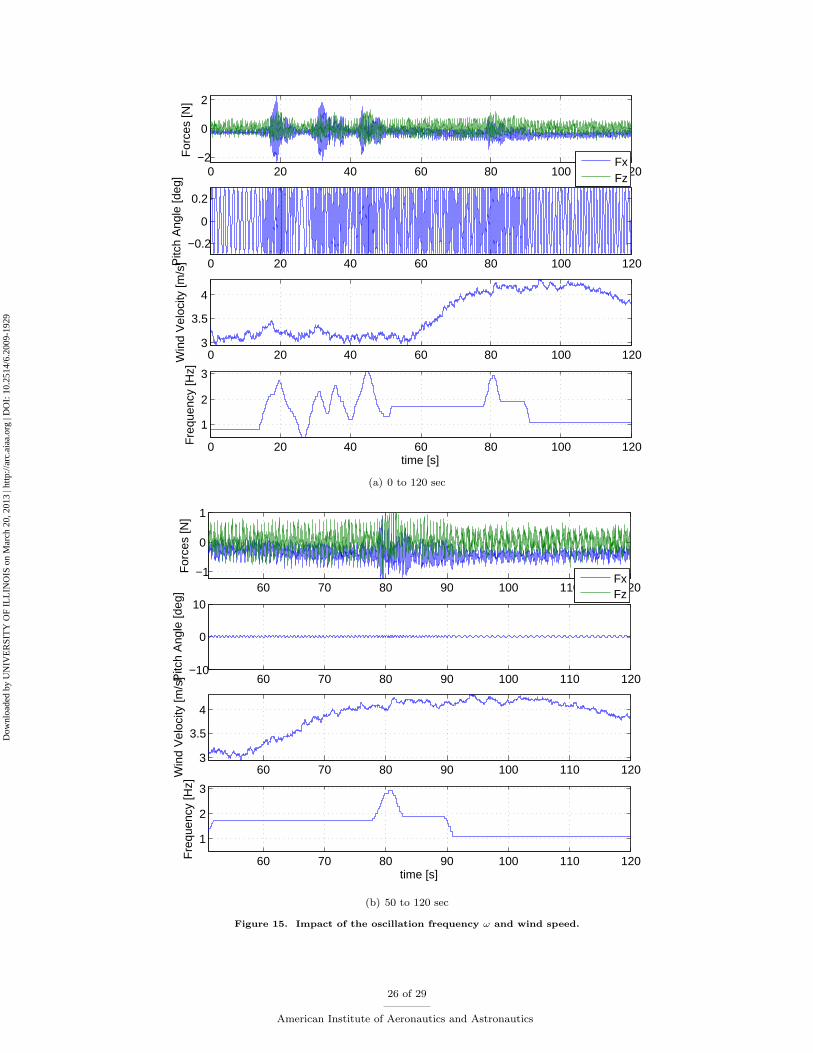
0 20 40 60 80 100 120−2
0
2
For
ces
[N]
FxFz
0 20 40 60 80 100 120
−0.2
0
0.2
Pitc
h A
ngle
[deg
]
0 20 40 60 80 100 1203
3.5
4
Win
d V
eloc
ity [m
/s]
0 20 40 60 80 100 120
1
2
3
time [s]
Fre
quen
cy [H
z]
(a) 0 to 120 sec
60 70 80 90 100 110 120−1
0
1
For
ces
[N]
FxFz
60 70 80 90 100 110 120−10
0
10
Pitc
h A
ngle
[deg
]
60 70 80 90 100 110 1203
3.5
4
Win
d V
eloc
ity [m
/s]
60 70 80 90 100 110 120
1
2
3
time [s]
Fre
quen
cy [H
z]
(b) 50 to 120 sec
Figure 15. Impact of the oscillation frequency ω and wind speed.
26 of 29
American Institute of Aeronautics and Astronautics
Dow
nloa
ded
by U
NIV
ER
SIT
Y O
F IL
LIN
OIS
on
Mar
ch 2
0, 2
013
| http
://ar
c.ai
aa.o
rg |
DO
I: 1
0.25
14/6
.200
9-19
29
controller we were able to conduct hardware-in-the-loop simulations using the CPG control laws. From thedata collected by this testing we are able to show that CPGs do allow for the smooth transitions of controlparameters, as well as generating useful wing trajectories.
The dynamic model and wing kinematic model of flapping flight were developed which represents themore complete and complex mechanical flapping system developed for wind tunnel testing. This dynamicmodel includes a tilted stroke angle, the lead-lag motion, and the relative body velocity, in addition to thestroke and pitch angles. The complete model includes all the degrees of freedom possessed by the roboticbat model.
Finally, the robotic bat model that has been developed provides a useful contribution to the state ofthe art. Previous models have been very limited by mechanical simplicity to generating only sinusoidalwaveforms. Our model allows not only allows experiments involving motions not used before such as leadlag, but also for experiments with non-sinusoidal waveforms. This bat model allows for additional researchinvolving compliant wings and other biologically inspired research. Coupled with the power of CPG controlthis allows for exploration of more sophisticated nonlinear flight control.
Acknowledgements
This project was supported by the Air Force Office of Scientific Research (AFOSR) under the YoungInvestigator Award Program (YIP) (contract monitor: Dr. Willard Larkin). This paper benefitted fromdiscussion with Profs. Jean-Jacques Slotine at MIT, Prof. Kenneth Breuer at Brown University, and Dr.Gregg Abate at the Air Force Research Lab. The first author appreciate Prof. Partha Sarka at Iowa StateUniversity for allowing him to use the wind tunnel facility in the Wind Simulation and Testing Laboratory.The authors gratefully acknowlege contributions from the following students at Iowa State University: AnidMonsur, Antonella Albuja, Brad Smith, Christopher Massina, Keegan Gartner, Matt Hawkins, MerrittTennison, and Ryan Paul.
References
1T. J. Mueller, e. a., Fixed and Flapping Wing Aerodynamics for Micro Air Vehicle Application, 2001, Progress inAstronautics and Aeronautics, AIAA.
2Shyy, W., Lian, Y., Tang, J., Viieru, D., and Liu, H., Aerodynamics of Low Reynolds Number Flyers, CambridgeUniversity Press, New York, NY., 2008.
3Azuma, A., The Biokinetics of Flying and Swimming, AIAA, 2nd ed., 2006.4Kato, N. and Kamimura, S., Bio-Mechanisms of Swimming And Flying: Fluid Dynamics, Biomimetic Robots, And
Sports Science, Springer Verlag, 2008.5Norberg, U. M., Vertebrate Flght: Mechanics, Physiology, Morphology, Ecology and Evolution, Springer-Verlag, 1989.6Dickinson, M. H., Lehmann, F. O., and Sane, S. P., “Wing Rotation and the Aerodynamic Basis of Insect Flight,”
Science, Vol. 284, 1999, pp. 1954–1960, June .7Swartz, S. M., “Allometric Patterning in the Limb Skeleton of Bats: Implications for the Mechanics and Energetics of
Powered Flight,” J. Morph., Vol. 234, 1997, pp. 277–294.8Swartz, S. M., Bishop, K. L., and Ismael-Aguirrre, M.-F., “Dynamic Complexity of Wing Form in Bats: Implications for
Flight Performance,” Functional and Evolutionary Ecology of Bats, Oxford University Press, Oxford, UK, 2005.9Dickinson, M. H., Lehmann, F. O., and Sane, S. P., “W,” Vol. 207, 1999, pp. 4269–4281, B. Dickinson and M. H.
Dickinson, “The effect of advance ratio on the aerodynamics of revolving wings,” Journal of Experimental Biology.10Ellington, C., “The Aerodynamics of Hovering Insect Flight. I-VI,” Philosophical Transactions of the Royal Society of
London B Biological Sciences, Vol. 305, 1984, 1181, .11Hall, K. C., Pigott, S. A., and Hall, S. R., “Power Requirements for Large-amplitude Flapping Flight,” Journal of
Aircraft , Vol. 35, No. 3, 1998, pp. 352–361.12Willis, D. J., Peraire, J., Drela, M., and White, J. K., “A Numerical Exploration of Parameter Dependence in Power
Optimal Flapping Flight,” 2006, pp. 2006–2994, AIAA.13Wang, Z. J., “Aerodynamic Efficiency of Flapping Flight: Analysis of a Two-stroke Model,” The Journal of Experimental
Biology, Vol. 211, 2008, pp. 234–238.14B. Roget, J. Sitaraman, R. H. J. G. J. C. J. H. and Humbert, S., “A Computational Study of Flexible Wing Ornithopter
Flight,” Proc. of the 26th Applied Aerodynamics Conference, 2008, Honolulu, HI, AIAA 2008-6397.15R. J. Albertani, B. Stanford, R. D. J. P. H. and Ifju, P., “Wind-tunnel Testing and Modeling of a Micro Air Vehicle with
Flexible Wings,” Journal of Aircraft , Vol. 35, No. 3, 2008, pp. 1025–1032.16Ho, S., Nassef, H., Pornsinsirirak, N., T., Y.-C., and Ho, C.-M., “Unsteady Aerodynamics and Flow Control for Flapping
Wing Flyers,” Vol. 39, 2003, Progress in Aerospace Sciences 635681.17Swartz, S. M., Iriarte-Diaz, J., Riskin, D. K., Song, A., Tian, X., Willis, D. J., and Breuer, K. S., “Wing Structure and
the Aerodynamic Basis of Flight in Bats,” Proc. of the 45th AIAA Aerospace Science Meeting, 2007, Reno NV.
27 of 29
American Institute of Aeronautics and Astronautics
Dow
nloa
ded
by U
NIV
ER
SIT
Y O
F IL
LIN
OIS
on
Mar
ch 2
0, 2
013
| http
://ar
c.ai
aa.o
rg |
DO
I: 1
0.25
14/6
.200
9-19
29
18X. Tian, K. Breuer, e. a., “Direct Measurements of the Kinematics and Dynamics of Bat Flight,” Bioinsp. Biomim.,Vol. 1, 2006, S10-S19.
19Deng, X., Schenato, L., Wu, W. C., and Sastry, S. S., “Flapping Flight for Biomimetic Robotic Insects: Part I-systemModeling,” IEEE Trans. on Robotics, Vol. 22, No. 4, 2006, pp. 776–788.
20Deng, X., Schenato, L., Wu, W. C., and Sastry, S. S., “Flapping Flight for Biomimetic Robotic Insects: Part II-flightControl Design,” IEEE Trans. on Robotics, Vol. 33, No. 4, 2006, pp. 789–803.
21Frampton, K. D., Goldfarb, M., Monopoli, D., and Cveticanin, D., “Passive Aeroelastic Tailoring for Optimal FlappingWings,” Fixed and Flapping Wing Aerodynamics for Micro Air Vehicle Application, 2001, pp. 473–482, T. J. Mueller, Ed.,AIAA,.
22Issac, K. K. and Agrawal, S. K., “An Investigation Into the Use of Springs and Wing Motions to Minimum the PowerExpended by a Pigeon-sized Mechanical Bird for Steady Flight,” Journal of Mechanical Design, Transactions of the ASME ,Vol. 129, 2007, .
23Jones, K. D., Lund, T. C., and Platzer, M. F., “Experimental and Computational Investigation of Flapping WingPropulsion,” Fixed and Flapping Wing Aerodynamics for Micro Air Vehicle Application, 2001, pp. 307–336, T. J. Mueller, Ed.,AIAA,.
24Kawamura, Y., Souda, S., Nishimoto, S., and Ellington, C. P., “Clapping-wing Micro Air Vehicle of Insect Size,” Bio-Mechanisms of Swimming and Flying: Fluid Dynamics, Biomimetic Robots, and Sports Science, Springer Verlag, 2008, pp.319–330, N. Kato and S. Kamimura, Ed.
25Larijani, R. F. and DeLaurier, J. D., “A Nonlinear Aeroelastic Model for the Study of Flapping Wing Flight,” Fixed andFlapping Wing Aerodynamics for Micro Air Vehicle Application, AIAA, 2001, pp. 399–428, T. J. Mueller, Ed.
26Michelson, R., Helmick, D., Reece, S., and Amarena, C., “A Reciprocating Chemical Muscle (RCM) for Micro Air VehicleEntomopter Flight,” Proc. of the Association for Unmanned Vehicle Systems, International , 1997, pp. 429–435.
27Steltz, E., Avadhanula, S., and Fearing, R. S., “High Lift Force with 275 Hz Wing Beat in MFI,” IEEE Int. Conf. onIntelligent Robots and Systems, 2007, San Diego, CA.
28Wood, R. J., “The First Takeoff of a Biologically-inspired At-scale Robotic Insect,” IEEE Trans. on Robotics, Vol. 24,No. 2, 2008, pp. 341–347.
29Taylor, G. K. and Zbikowski, R., “Nonlinear Time-periodic Models of the Longitudinal Flight Dynamics of Desert LocustsSchistocerca Gregaria,” J. R. Soc. Interface, Vol. 2, 2005, pp. 197–221.
30Zbikowski, R., Ansari, S. A., and Knowles, K., “On Mathematical Modelling of Insect Flight Dynamics in the Contextof Micro Air Vehicles,” Bioinsp. Biomim., Vol. 1, 2006, pp. 26–37.
31Birch, J. and Dickinson, M., “Spanwise Flow and the Attachment of the Leading-edge Vortex on Insect Wings,” Nature,Vol. 412, Aug . 2001, pp. 729–733.
32T. Pornsinsirirak, S-W. Lee, H. N. J. G. Y.-C. T. C.-M. H. M. K., “MEMS Wing Technology for a Battery-poweredOrnithopter,” Proceedings of the International Conferences on MEMS , 2000, pp. 709–804, Miyazaki, Japan.
33Jadhav, G., The Development of a Miniature Flexible Flapping Wing Mechanism for Use in a Robotic Air Vehicle, 2007,M.S. Thesis, Georgia Institute of Technology, Atlanta, GA.
34Bay, J. S. and Hemami, H., “Modeling of a Neural Pattern Generator with Coupled Nonlinear Oscillators,” IEEE Trans.on Biomedical Engineering, 1987.
35Bernstein, N., The Coordination and Regulation of Movements, Pergamon Press, Oxford, 1967.36Collins, J. J. and Stewart, I. N., “Coupled Nonlinear Oscillators and the Symmetries of Animal Gaits,” Nonlinear Science,
Vol. 3, 1993, pp. 349–392.37Golubitsky, M., Stewart, I., Buono, P., and Collins, J., “Symmetry in Locomotor Central Pattern Generators and Animal
Gaits,” Nature, Vol. 401, No. 19, 1999, pp. 693–695.38Hooper, S. L., “Central Pattern Generators,” In Nature Encyclopedia of Life Sciences, 2001, London, Nature Publishing
Group.39Hooper, S. L., Guschlbauer, C., von Uckermann, G., and Buschges, A., “Natural Neural Output That Produces Highly
Variable Locomotory Movements,” J. Neurophysiology, Vol. 96, 2006, pp. 2072–2088.40Lewis, M. A., Tenore, F., and Etienne-Cummings, R., “CPG Design Using Inhibitory Networks,” Proc. of the 2005 IEEE
Int’l Conference on Robotics and Automation, 2005, pp. 3682–3687, Barcelona, Spain.41Matsuoka, K., “Mechanisms of Frequency and Pattern Control in Neural Rhythm Generators,” Biological Cybernetics,
Vol. 56, 1987, pp. 345–353.42Sekerli, M. and Butera, R. J., “Oscillations in a Simple Neuromechanical System: Underlying Mechanisms,” Journal of
Computational Neuroscience, Vol. 19, No. 2, 2005, pp. 181–197.43Marder, E. and Calabrese, R. L., “Principles of Rhythmic Motor Pattern Production,” Physiological Reviews, Vol. 76,
1996, pp. 687–717.44Grillner, S., “Neurological Bases of Rhythmic Motor Acts in Vetebrates,” Science, Vol. 228, 1985, pp. 143–149.45Zheng, T. I. M., “Sensory Feedback Mechanism Underlying Entrainment of Central Pattern Generator to Mechanical
Resonance,” Biological Cybernetics, Vol. 94, No. 4, 2006, pp. 245–261.46Seo, K., Chung, S.-J., and Slotine, J.-J. E., “CPG-based Control of a Turtle-like Underwater Vehicle,” Proc. of the
Robotics: Science and Systems (RSS), 2008, Switzerland.47Ijspeert, A. J., “Central Pattern Generators for Locomotion Control in Animals and Robots: A Review,” Neural Networks,
Vol. 24, No. 4, 2008, pp. 642–653.48Ayers, J. and Rulkov, N., “Controlling Biomimetic Underwater Robots With Electronic Nervous Systems,” Bio-
Mechanisms of Swimming and Flying: Fluid Dynamics, Biomimetic Robots, and Sports Science, Springer Verlag, 2008, pp.295–306, N. Kato and S. Kamimura, Ed.
49Ijspeert, A. J., Crespi, A., and Cabelguen, J.-M., “Simulation and Robotics Studies of Salamander Locomotion: ApplyingNeurobiological Principles to the Control of Locomotion in Robots,” Neuroinformatics, Vol. 3, No. 3., 2005, pp. 171–195.
28 of 29
American Institute of Aeronautics and Astronautics
Dow
nloa
ded
by U
NIV
ER
SIT
Y O
F IL
LIN
OIS
on
Mar
ch 2
0, 2
013
| http
://ar
c.ai
aa.o
rg |
DO
I: 1
0.25
14/6
.200
9-19
29
50Morimoto, J., Endo, G., Nakanishi, J., and Cheng, G., “A biologically inspired biped locomotion strategy for humanoidrobots: modulation of sinusoidal patterns by a coupled oscillator model,” 2006.
51Strogatz, S., Nonlinear Dynamics and Chaos With Applications to Physics , Biology, Chemistry, and Engineering,Perseus Books Group, Cambridge, MA, 1994.
52Slotine, J.-J. E. and Li, W., Applied Nonlinear Control , Prentice Hall, 1991.53Pham, Q.-C. and Slotine, J.-J. E., “Stable Concurrent Synchronization in Dynamic System Networks,” Neural Networks,
Vol. 20, No. 1, 2007, pp. 62–77.54Chung, S.-J. and Slotine, J.-J. E., “On Global Synchronization of Coupled Hopf-Kuramoto Nonlinear Oscillators,” 2009,
submitted.55Norberg, U. M. and Winter, Y., “Wing Beat Kinematics of a Nectar-feeding Bat, Glossophaga Soricina, Flying At
Different Flight Speeds and Strouhal Numbers,” J. of Experimental Biology, Vol. 209, 2006, pp. 3887–3897.56Taga, G., “A Model of the Neuro-musculo-skeletal System for Anticipatory Adjustment of Human Locomotion During
Obstacle Avoidance,” Biological Cybernetics, Vol. 78, No. 1, 1998, pp. 9–17.57Doya, K., Kimura, H., and Kawato, M., “Neural Mechanisms of Learning and Control,” IEEE Control Systems Magazine,
Vol. 21, No. 4, 2001, pp. 42–54.58Riskin, D. K., Willis, D. J., Iriarte-Diaz, J., Hendrick, T. L., Kostandov, M., Chen, J., Laidlaw, D. H., Breuer, K. S., and
Swartz, S. M., “Quantifying the Complexity of Bat Wing Kinematics,” J. of Theoretical Biology, Vol. 254, 2008, pp. 604–615.59Chung, S.-J. and Slotine, J.-J. E., “Cooperative Robot Control and Concurrent Synchronization of Lagrangian Systems,”
IEEE Transactins on Robotics, Vol. 25, No. 3, 2009.60Lohmiller, W. and Slotine, J.-J. E., “Contraction Analysis for Nonlinear Systems,” Automatica, Vol. 34, No. 6, 1998,
pp. 683–696.61Iwasaki, T. and Zheng, M., “What Makes Biological Oscillators Achieve Robust Self-excitation?” Vol. 2, 2003, pp. 1824–
1829, Proc. American Control ConferenceJune .62Taga, G., Yamaguchi, Y., and Shimizu, H., “Self-organized Control of Bipedal Locomotion by Neural Oscillators in
Unpredictable Environment,” Biological Cybernetics, Vol. 65, 1991, pp. 147–159.63Ijspeert, A. J., Crespi, A., Ryczko, D., and Cabelguen, J.-M., “From Swimming to Walking with a Salamander Robot
Driven by a Spinal Cord Model,” Science, Vol. 315, No. 5817, 2007, pp. 1416–1420.64Morimoto, J., Endo, G., Nakanishi, J., Hyon, S.-H., Cheng, G., Bentivegna, D., and Atkeson, C. G., “Modulation of
Simple Sinusoidal Patterns by a Coupled Oscillator Model for Biped Walking,” Proc. of the 2006 IEEE Int’l Conference onRobotics and Automation, 2006, pp. 1579–1584.
65MacMahon, T. A., Muscles, Reflexes, and Locomotion, 1984, Princeton University Press, .66Thomas, A. L. R. and Taylor, G. K., “Animal Flight Dynamics I. Stability in Gliding Flight,” J. Theor. Biol., Vol. 212,
2001, pp. 399–424.67Taylor, G. K. and Thomas, A. L. R., “Animal Flight Dynamics II. Longitudinal Stability in Flapping Flight,” J. theor
Biol., Vol. 214, No. 3, February 2002, pp. 351–370.68Swartz, S. M., Groves, M. S., Kim, H. D., and Walsh, W. R., “Mechanical Properties of Bat Wing Membrane Skin,”
Journal of Zoology, Vol. 239, 1996, pp. 357–378.
29 of 29
American Institute of Aeronautics and Astronautics
Dow
nloa
ded
by U
NIV
ER
SIT
Y O
F IL
LIN
OIS
on
Mar
ch 2
0, 2
013
| http
://ar
c.ai
aa.o
rg |
DO
I: 1
0.25
14/6
.200
9-19
29