Embed Size (px)
Citation preview

New algorithms and methods for protein and DNA sequence comparison
James Crook
A Thesis Presented for the Degree of
Ph.D.
Biocomputing Research Unit, Department of Molecular Biology, University of Edinburgh.
May 1991.

Abstract International biological sequence databases hold information about protein
and DNA molecules. The molecules are represented by sequences of characters. In analysis of this data algorithms for comparing the character sequences play a central role. Comparisons can be made using dynamic programming techniques to determine the score of optimal sequence alignments. Such methods are particularly popular with molecular biologists for they accommodate the kinds of differences which actually occur in the sequences of related molecules.
Sequence alignments are normally scored using score tables based on an evolutionary model. The derivation of these score tables is re-examined and a formula giving an analytic counterpart to an empirical method for assessment of a score table's discriminating power is found. Use of the formula to derive alternative protein similarity scoring tables is discussed.
A new approach to tackling the heavy computational demands of the dynamic programming algorithm is described: intensive optimisation of a microcomputer implementation. This provides an alternative to implementations which use parallel computers for searching protein databases. This thesis also describes how other implementational problems were tackled in order to make more effective use of the serial comparison software.
The new software permitted comparison by optimal alignment of 32,000,000 pairs of sequences from a protein database using widely available and inexpensive hardware. The results from this search were then reorganised to facilitate the finding of previously unseen similarities. Software tools were written to assist with the analysis including software to align sequence families.
From the results of this work, nine similarities are presented which do not appear to have been previously noted. The examples illustrate factors that are important in assessing similarities with scores close to the boundaries of significance. The similarities presented are of particular interest because of the biological functions they relate.
One software tool developed for the sequence analysis work was a new multiple sequence alignment editor and sequence aligner, "Medal". Lessons from its use on real sequence data lead to a modification to the original comparison method to accommodate local variations in sequence similarity.
Consideration is given to parallelisation of this modification and of the methods used to obtain speed in the serial software. Alternatives are suggested. The suggested parallel method to cope with variations in sequence similarity requires two interdependent sequence comparisons. A serial program using three interdependent comparisons is demonstrated and shows the feasibility of multiple interdependent comparisons. Examples show how this new program, "Fradho", can compare DNA sequences to protein sequences accommodating frameshifts.
I'

Acknowledgements
Firstly I thank my two supervisors. I particularly want to thank Professor
Sidney Michaelson (Computer Science) for his constructive criticism combined
with lively interest and encouragement. I wish he were still alive and that we
could talk about shared interests in Computer Science, Molecular Biology and
Mathematics. I also thank Dr John Collins (Molecular Biology) and I thank the
Science and Engineering Research Council for their funding.
There are many other people I want to thank too. I thank Andrew Lyall,
whose achievements in biological sequence analysis and enthusiasm encouraged
me to join in too; Duncan Rouch, who showed me the importance of comparative
testing; Dr Andrew Coulson for instruction in "0" and help with laser printer
problems; Ian Campbell for attempting, with intermittent success, to repair the
jinxed IBM PC clone; for making the computing unit more human, Carol Crawley,
Tom Smith, Alok Kumar, Steven Hayward and Sarah (SJ) McQuay whom I also
thank for comments on the draft; Adelaide Carpenter for showing me how to
copy edit on an early draft of Chapter 8; the excellent staff at the Darwin library
for all their help; Richard Hayward for comments on S. aureus protein-A; Stuart
Moodie for drawing my attention to a paper on the p53 antigen; Roger Slee for
providing dodgy DNA data at an early stage of sequencing; Michelle Ginsburg for
the viral subunit sequences to align; Gill Cowan for explaining the restriction
enzyme identification problem and Mike Holmes and Peter Cleat in the
computing support for biologists group. Finally I want to thank my parents, sister
and my girlfriend Bobby for all their encouragement. Any mistakes in this thesis
are of course my own, alas, in this instance blaming the computer does not help
me much.
111

Declaration
The following declaration is made in accordance with paragraph 3.4.7 of
the University of Edinburgh regulations governing the submission of theses.
I declare that this thesis has been composed by me and that all the work
described in it is my own unless clearly indicated otherwise.
James Crook
May 1991.
Edinburgh.
iv

Contents
Chapter 1: Introduction II Biological sequence data 1 Software for sequence analysis 13
• Importance of sequence comparison 13 Concluding remarks 16
Chapter 2: Comparison Methods and the NWS Algorithms 17 Word based comparison 17 Estimating likelihoods of chance matching 18 Alphabet reduction 20 Scoring amino acid similarity 21 Comparison by alignment 23
Chapter 3: Measuring Similarity 29 The Dayhoff model 30 Assumptions of the model 31 Justification for method for deriving 1 PAM table 38 Explanation for symmetry of A' 39 Discrimination of similarity scoring tables 40 Other amino acid similarity scoring tables 46
Chapter 4: Rapid and Sensitive Database Searching Sensitivity and selectivity 49 Computational cost 49 Database reduction 51 Approximate methods for comparison 54 Theoretical advances in comparison algorithms 56 Concluding remarks 57
Chapter 5: Techniques to Get More from Machines Type III comparison (speed) 58 Path reconstruction (memory space) 61 Database compression (disk space) 64 Tripeptide matching (speed) 66 Annotation browser (portability) 67 Optimisations to "Prosrch" 68 Concluding remarks 70
58
V

Chapter 6: Multiple Sequence Alignment
71 Uses of multiple alignments 72 Sequence editors 74 Automatic alignment methods 82 Use of the new computer tools 88 Concluding remarks 91
Chapter 7: Comprehensive Database Analysis
93 Organisation of sequence data 93 Methods and data used in comprehensive search 94 Reduction of the similarity data 97 Tree formation 100 Examining results 101 Concluding remarks 109
Chapter 8: Twilight Zone Similarities Scores to significances 112 Repetitive sequence problem: Protein-A 114 Weak local constraints 116 Viral repetitive proteins 117 Local similarity and local structure 118 Multiple matching: An AMP binding pattern? 119 Conserved cysteines: Two plasma proteins 122 Similarities across taxonomic boundaries 123 Two pathogenesis related proteins 124 Protein formation and folding 125 Arginosuccinate and two viral proteins 126 Phosphoenolpyruvate -regulated sugar transport 127 Concluding remarks 127
Chapter 9: NWS variants 129 Coding regions and frameshifts 129 "Fradho" 131 Variations in noise 140 Mixed noise Type III comparison 142
111
v

Addendum: The "Blast" algorithm 144 "Blast's" method for finding word-pairs 145 Validity of seed based matching 146
Appendix 1: Tests of some ideas for new software 147 Introduction 147 Sequence retrieval 147 Dotplots 149 Identification of a target pattern 151
Appendix 2: Methods for fast serial type III comparison 154
Appendix 3: Conditional deferred assignment 161
Appendix 4: Potential for optimisations to "Prosrch" 163
Abbreviations 168
References 170
VII

Chapter 1: Introduction
This interdisciplinary thesis seeks to improve the ways in which Information
Technology is applied to the analysis of biological sequence data. This is
simultaneously a theoretical and a practical problem. The approach taken in this
work is a pragmatic one. Both the nature of the data being studied and practical
computational issues need to be considered. We start by describing the nature of
biological sequence data, how this information represents biological molecules and
how these molecules relate to genetic information, the information held in cells
that is passed on when cells divide.
Biological sequence data
Polymeric macromolecules synthesised within cells are fundamental to the
chemical processes on which all life depends. During the last two decades
molecular biologists have characterised many thousands of these macromolecules.
The chemical structures they have determined are conveniently represented by
sequences of characters. These sequences, the biological sequence data, have
been collected on an international scale to make biological sequence databases
(Barker et al., 1990; Kahn & Cameron, 1990; Burks et al., 1990).
Two classes of macromolecule are represented in the databases. One class
is the protein molecules. Proteins are polymers of amino acids. The other class
is the deoxyribonucleic acid (DNA) molecules. DNAS are polymers of nucleotide
monomers. Structural and other information about the component monomers of
proteins and DNAS is given, mostly in diagramatic form, in figures 1.1 to 1.4.
These diagrams are explained in greater detail in later sections of this chapter.
Both proteins and DNAs are linear polymers. The order of characters in
the sequences representing a protein or DNA molecule corresponds with the
order in which monomers form the linear polymer chain.
As well as holding protein and DNA sequence data, the databases contain
textual information. The textual information describes the known roles of the
1

molecules and gives references to the literature in which the sequence data were
reported.
Genetic information
Collecting information about DNAs and proteins is an essential part of the
process of investigating how organisms function at the molecular level. The
chemical reactions in a cell form a highly complex organised system. Multi-stage
metabolic pathways convert chemical resources available to a cell into forms that
meet the cell's current needs. Protein molecules are crucial to such pathways. In
a typical pathway, each reaction is catalysed by a specific protein. Genetic
information specifies the kinds of protein synthesised by the cell and hence it
determines the metabolic pathways.
The structure of a protein determines how it interacts with other molecules.
Taking a specific example, some chemical groups at the surface of a protein may
be arranged so that they readily bind to a comparatively small molecule,
adenosine triphosphate (ATP). ATP is an important carrier of readily available
energy. By specifying the chemical structures of proteins synthesised in the cell,
genetic information determines how chemical energy is used.
Like chemical energy, genetic information is vital to the cell. Accurate
information is essential to the correct functioning of cellular chemistry. A
bacterial cell such as Escherichia coli holds genetic information that precisely
specifies over 3000 different proteins each of which is formed from, on average,
300 amino acids. Cells also carry information to regulate the synthesis of proteins,
to ensure that under differing conditions that the appropriate quantity of each
protein is made. Just as there are molecules which carry chemical energy, so too
there are molecules which carry genetic information. Molecules of DNA are the
primary carriers of genetic information. DNA carries the information which
specifies the proteins.
With the discovery of the double helical structure of DNA (Watson &
Crick, 1953), the manner in which cells pass on genetic information to their
progeny became clear for the first time. The paired structure of DNA suggests
a biochemical mechanism for replication of DNA. Chemical processes in the cell
2

make precise copies of DNA molecules thus passing information on to the cell's
descendants.
Other achievements fundamental to the discipline of Molecular Biology
followed the discovery of DNA's structure. These included development of
techniques by Sanger et al. (1977), to rapidly determine base sequences of DNA
molecules. These techniques make it possible for molecular biologists to read
genetic information encoded in DNA. Over the years these techniques have been
used extensively and refined. Much molecular biological research can be viewed
as experimental work aimed at understanding the function of the data encoded
in different DNA molecules.
A landmark achievement in the interpretation of DNA sequence data has
been the elucidation of one of the basic information encoding strategies used by
DNA, the so called 'genetic code' (Frisch, 1966). Using a table giving the genetic
code it is now possible to deduce the.sequence of amino acid residues of a protein
from the DNA sequence that encodes it.
We now briefly describe the molecules, proteins and DNAS, that are
represented by sequence data. We then describe the link between the two classes
of molecule. More extensive information can be found in standard texts on
Molecular Biology such as Lewin's "Genes" (1990).
DNAS
The now famous DNA double helix consists of a pair of antiparallel
complementary strands of deoxyribonucleic acid. Each strand is a linear polymer
of thousands of nucleotide monomers. The nucleotides are similar in a sugar-
phosphate part which makes the 'backbone' of the strand. They differ in a
nitrogenous chemical group called a base. Information is carried by the sequence
in which the bases occur along a single strand's length. Four characters c, t, a and
g, are used in the sequence representation. They represent the four bases
cytosine, thymine, adenine and guanine. The order of characters in a sequence
corresponds with the order of chemical groups in one strand.
The bases come in complementary pairs; c pairs with g and t pairs with a.
Where one strand has c the complementary strand has g and similarly for each of
3

the other three possibilities. The pairing arises because the individual bases can
form stable interactions with their specific partner through weak 'hydrogen
bonding'. Hydrogen bonding of bases is shown in figure 1.1. This figure also
shows the chemical structure of the four bases. Only one strand of each double-
stranded DNA molecule is represented in the databases since the complementary
strand can be deduced from its partner. The complementary pairing of two
strands is both the basis for the stability of double stranded DNA as a molecule
and also the basis of the mechanism of information preserving replication of
DNA.
Cytosine Guanine H -H I I I 10
C_
7N / C\ _
/ C\
/ H-C
N-C
C-N I H-N /
NC-\.
/ \ /__ N CII 11
H
Adenine Thy nine
H OIIIIH-N'
H'
' \ C C C-H
/ C- N
/ C \ H/ 0
Figure 1.1: Hydrogen bond formation between complementary base pairs.
Proteins
Protein sequences have greater prominence in this work than do DNA
sequences. Whereas DNA is the information carrier, proteins are the active
expression of this information. Proteins are linear polymers of twenty kinds of
amino acid.
4

Like DNA character sequences, protein character sequences represent the
order of simple subunits of a polymeric macromolecule. Protein sequences vary
in length from a few tens of characters (e.g. some hormones) to several thousand
characters (e.g. viral polyproteins). Each character in the sequence represents an
amino acid residue. The term 'residue' is used here to denote the parts of the
amino acid left after the polymerisation reaction is complete. In the reaction the
crb jiciroup of one amino acid reacts with the amino group of the next (figure
1.4). The residue of the amino acid consists of atoms involved in the protein
backbone plus a side-chain characteristic of the amino acid. The side-chains are
illustrated in figure 1.3. Proteins of around thirty or fewer residues are sometimes
referred to as polypeptides, or just peptides, for the bond between residues is
known as a peptide bond.
Unlike DNAs, proteins are single stranded polymers. Proteins fold into
complex three dimensional structures due to side-chain interactions (Schulz &
Schirmer, 1979). Aromatic residues, Phe, Trp, Tyr ; and aliphatic residues, Ile, ,4)a
Leu, Val, have hydrophobic water repelling side-chains (Taylor, 1987a). Protein
folding, at least in an aqueous environment, is largely driven by a reduction in
energy through hydrophobic residues becoming buried in the core of the structure.
Two particular kinds of region of regular substructure are frequently found
in proteins. These are near planar zig-zag substructures (beta sheet), and helical
substructures (alpha helix). Both these sub-structures are characterised by a
regular pattern of hydrogen bonding involving atoms of the protein backbone.
The folded structure adopted by the protein is energetically favourable, that is,
slight perturbations of the structure have higher energy and are less stable. The
folded structure is essential to the protein's biochemical activity. The regular sub-
structures are crucial to the formation and stability of the folded molecule.
Frequently there is biologically significant modification of these basic
structures. The folded structure may be further stabilised by the formation of
covalent 'disulphide bridges' between cysteine residues in different regions of the
sequence that have been brought close together by the folding. Other residues
on the surface of the protein may also be chemically modified. However, three
dimensional structure is essentially dependent on the sequence.
5

Amino Acid Abbr. Symbol Frequency
Glycine Gly G 0.089
Alanine Ala A 0.087
Leucine Leu L 0.085
Lysine Lys K 0.081
Serine Ser S 0.070
Valine Val V 0.065
Threonine Thr T 0.058
Proline Pro P 0.051
Glutamic acid Glu E 0.050
Aspartic acid Asp D 0.047
Arginine Arg R 0.041
Asparagine Asn N 0.040
Phenylalanine Phe F 0.040
Glutamine Gin 0 0.038
Isoleucine lie I 0.037
Histidine His H 0.034
Cysteine Cys C 0.033
Tyrosine Tyr Y 0.030
Methionine Met M 0.015
Tryptophan Trp W 0.010
Figure 1.2: The amino acids and their standard three letter and one letter abbreviations. The list is in order of abundance, glycine being most abundant and tiyptophan being least abundant. After Dayhoff et al. (1978).
1.1

•
H( ;CH
CH CH2 H2 H2
HNH
Pro -P- His -H- Trp -N- Tyr -I- Phe -F-
1 1 1 H H-C-H H-C--H H-C-H
t I I I I I H-C-- C-H H-C--H H-C-H H- C-H H--C-H
H-C-H H H-C-H H-C-H I
S
I S
I I H-t --H
I H-t --H H-N H-C--H H
I H
I NH3
I CNH2
I H
H// NH
Ile -I- Lys -K- Arg -R- Met -H- Cys -C-
i I I I.
H-C-H H-(-H H--H H-c--OH
I I H H H-C-H H-C--H H-C-H
I H-C---H
I I H- --c-H
I I H H
Leu -L- Gin -Q- Giu -E- Thr -T- Ala -A-
I I H H H-C-H H-C-H W-O-OH
I I I H H H-C_-C--H CN
Val -V- ASn -N- Asp -D- Ser -5- Gly -G-
Figure 1.3: The characteristic side chains of different amino acids. These have been arranged in an unconventional way to emphasize some of the similarities and differences. For example, side chains in row 3 differ to those in row 4 only by addition of an extra carbon group. The similarities of individual amino acid types are crucial to comparison ofprotein sequences with sensitivity.
7

H3 C
H-C-H
H-C-H
4 H-C-H
+ H3N—c
H
+ / \ •••••'O-
HCH HCH
+ H3N-
H-C--OH
Methionine + Glycine + Praline + Serine
H 0 H 0 H 0 H 1 II I II. I II 1 0 H3N— C— C—N- C—C—N-C—C—N-C—Cd
H-C-H H H HCH HCH H H-C-OH
H-C-H C H H
H-C--H + 3H20
Figure 1.4: Polymerisation of amino acids to form a polypeptide.
Protein synthesis
The folded proteins have an astonishingly diverse range of functions,
structural, regulatory and catalytic. Proteins with catalytic roles are particularly
important to cellular chemistry. They are known as 'enzymes'. Enzymes are
powerful and highly specific catalysts.
Proteins, whether enzyme or otherwise, are the key intermediate stage by
which information held in DNA specifies the functioning of the cell. Chemical
processes studied in Molecular Biology either involve proteins directly or have
proteins catalysing the reactions.

In regions of DNA that code for protein a run of three consecutive bases
is used to specify selection of one amino acid. Three bases gives 64 Possibilities
rather than twenty. The encoding scheme has redundancy in it; several
possibilities usually encode the same amino acid.
DNA is not translated directly. Instead a ribonucleic acid (RNA) copy of
the DNA sequence is made, a process called 'transcription'. RNA is very similar
to a single strand of DNA except uracil, a base like thymine but lacking a methyl
group, is used in place of thymine and the sugar is ribose instead of deoxyribose.
Instructions in an RNA transcript are read as a protein is formed in a process
called 'translation'. This process of precisely controlled polymerisation takes place
in complex assemblies, the ribosomes, which are themselves made from protein
and RNA molecules.
2nd base
44
-C S. C.
p..
Co
eel
Figure 1.5: The coding scheme wherekv triples of adjacent bases (codons) code for individual amino acids. indicate stop codons, the end of a translated section. The code is presented in the alphabet of RNA in which u substitutes for t. To produce proteins, a short transcript of RNA is first produced from the DNA master copy. The residues shown shaded are those encoded by three or more different codons. The organisation and shading of this table are non-standard and draw attention to a pattern in the code which involves codons whose second base is a.
2

The diversity in proteins is achieved with great economy. The same
molecular machinery driven from different sets of instructions is used in
synthesising all proteins. It is variation in the sequences of the amino acid
subunits, rather than a wide range to the subunits themselves, that give proteins
their profoundly different properties.
Software for sequence analysis
• Software for sequences analysis can be used to compare any newly
determined protein or DNA sequence to sequences in the databases. This is a
vital step in relating new information to information that is already known. When
an unexpected new similarity is found between sequences, it can lead to a
• hypothesis about the processes taking place in cells. The hypothesis can then be
tested by experiment. As an example, one similarity discovered by a computer
database search linked proteins that stimulate cell growth (growth factors) and
proteins implicated as causative agents in cancer (oncogenes) (Doolittle et al.,
1983). A number of different examples of growth factor and oncogene similarities
are now known. The discovery of this link has been of great interest to
researchers as it gives insight into the molecular mechanism whereby oncogenes
lead to uncontrolled growth (Bradshaw, 1987).
Computers are of importance in other aspects of sequence analysis work
in addition to their role in database searching. One of the most widely used
software packages for biological sequence analysis, at least in universities, is the
genetics computer group (GCG) package originally written at the university of
Wisconsin (Devereux et al., 1984). The GCG package provides a wide range of
sequence analysis facilities from simple programs that reverse and complement a
DNA sequence to derive the sequence of one DNA Strand from its
complementary pair, to computationally demanding programs that attempt to
predict some structural aspects of RNA molecules. The distributors of the
software have a policy of making source code for all these progranis available.
This makes it possible to adapt GCG programs to test out new sequence analysis
ideas. The package provides a natural base from which to develop flew ideas for
sequence analysis.

Applied information technology
How can one develop new algorithms that will actually help molecular
biologists? It is important that algorithms are genuinely of use, rather than solving
problems so idealised that they bear little relation to biologists' requirements.
Three approaches are considered.
1) Firstly, one may be able to identify aspects of sequence analysis which
have been consistently neglected by software developers. One area that has been
neglected is the combined use of both DNA and protein information.
Most analysis software deals independently with DNA data or with protein
data, except when translating to or from DNA. Analysis programs therefore
encourage researchers to see DNA and protein properties as independent, not to
look for relationships between them. There is, however, interest in analyses that
relate the two kinds of data.
One hypothesis where examination of both DNA and protein sequences is
important concerns introns and protein domains. Introns are stretches of nucleic
acid sequence which are removed from RNA before translation. Protein domains
are independently folding functional regions within a protein. A hypothesis that
links introns and boundaries between protein domains (Gilbert, 1978) is one of
several that attempt to explain the presence of introns. Under this hypothesis
introns separate functional domains and facilitate their rearrangement to make
multifunctional proteins. Such a mechanism may underlie patterns of similarity
actually observed in protein molecules (Patthy, 1985).
A second example where an interplay between DNA and protein
properties is important concerns the use of rare codons. Some codons for the
same amino acid residues are used preferentially to others. Use of the rarer
codons causes pauses in translation (Varenne et al., 1984) which may facilitate
protein folding. Whilst codon usage for whole DNA sequences can be tabulated,
software tools, as they currently stand, do not encourage investigation of such
hypotheses.
Those two examples are somewhat specialised. However, there is a
frequently required analysis in which consideration of both DNA and protein
11

sequences is important. Currently in searching databases researchers use either
DNA sequences or use the derived protein sequences. The problems this causes
are considered in Chapter 9 where software that simultaneously uses both
translated and untranslated DNA is presented.
A second approach to applying Information Technology is to examine
existing computer sequence analysis tools that have proved their worth and to
improve them. This may involve making a program run faster, making it perform
a more comprehensive analysis or provision of a new interface that makes a
cumbersome investigation more straightforward.
A third approach is to start from specific analysis problems that
molecular biologists find are difficult to solve using existing tools. Either a
satisfactory way can be found using a combination of existing tools, or new
methods can be developed.
All three approaches have their uses. The approaches reinforce each other
since new methods, improvements and difficult analyses influence the design of
new software. It was the combined use of these approaches, new ideas being
tested by writing new software, that directed research in this thesis.
In the early stages of the work a number of ideas and test implementations
of programs were tried. Also time was spent helping biologists new to the GCG
package with specific analysis problems. Some individual software ideas and
conclusions from this work are summarised in Appendix 1. This summary
illustrates some of the current practical difficulties with existing sequence analysis
software. These early investigations helped to focus further research by drawing
attention to the importance of sequence comparison in sequence analysis work.
12

Importance of sequence comparison
Comparison of biological sequences is fundamental to Computational
Molecular Biology. It is possibly the most useful computational technique
available. Why should this be so?
Firstly, comparison is required in database searches. Comparison allows
new sequence data to be related to previously studied sequences. Similarity in
sequences may give a researcher insight into a previously unsuspected function.
Comparison of a sequence to sequences in a database allows the researcher to
draw on a large collection of information that is frequently being updated.
Secondly, comparison of sequences which are already known to be related
shows patterns of similarity and differences. Most regions of related sequences
show some changes. Some regions show a remarkable stability. Sequence
comparison can draw attention to these conserved regions. One can hypothesise
that in these regions the evolutionary process has eliminated organisms which
show variation. If so, this suggests that the regions have crucial biochemical
functions requiring precise spatial organisations of amino acid residues.
Comparison which reveals conserved regions can therefore act as a guide to
identification of the site where an enzyme interacts directly with a substrate, the
active site. This can guide an experimenter, increasing the chance of identifying
by experimental techniques crucial regions early in their study.
Comparison software is also used to organise experimental data. In
experimental work to determine a DNA sequence many fragmentary sequences
are collected. Overlaps between these need to be found so that a long consensus
sequence can be determined. Organising the fragments into a longer sequence
requires comparison.
Underlying the various applications of sequence comparison is a common
theme. Comparison is a first stage in organising information. In biological
sequence database searching, comparison selects and brings to the attention of
researchers information that is most likely to be relevant. The comparisons bring
related sequences together whatever their order in the database. In studies of
related sequences, comparisons organise the differences and similarities so that
patterns of similarity can be seen.
13

Alternatives to sequence comparison
The three dimensional structure of a protein, as for example deduced from
X-ray crystallographic data, gives information about the arrangement in three
dimensions of the atoms of the molecule. In contrast, chemical structures only
give information about covalent bonding. Chemical structures give selective
information about the distances between atoms. Where the word 'structure' is
not qualified by 'chemical' in this thesis, we are referring to three dimensional
structure.
Comparison of protein structures should give a more accurate method for
investigating shared function than does sequence comparison alone. Function may
depend on the precise arrangement of residues in a small patch at the surface of
the protein. Residues which are close in the folded protein will not necessarily be
close in the linear sequence.
However, structural comparison techniques have limited applicability. Only
a few hundred distinct protein structures are known whereas many thousands of
protein sequences have been obtained (Pallabiraman et al., 1990). This reflects
the difficulty of obtaining protein structures. Determination of a structure using
X-ray crystallographic techniques is only possible where the protein can be
crystallised. The newer and more rapid nuclear magnetic resonance (NMR)
structure determining techniques also have limitations, particularly as regards the
size of molecules that can be analysed (Gronenborn & Clore, 1989).
Were it possible to deduce protein structure directly from sequence,
sequence comparison would have far less importance. Structural rather than
sequence comparisons would be of greater interest to researchers attempting to
understand protein function. Attempts have therefore been made to apply
computers to the problem of deducing protein structures from protein sequences.
Predicting structure from sequence
Protein structure prediction from sequence data alone presents a
formidable problem. Each structure for a protein has a corresponding energy.
The energy depends to a large extent on hydrogen bond formation. Calculating
the structure of minimum energy for a protein of known chemical structure
14

involves minimisation of a non-linear energy function involving thousands of
variables. Approaches to the problem so far have met with very limited success.
Simulations of protein folding and use of current energy minimisation techniques
suffer from phenomenal computational demands. There is uncertainty too about
whether the structure a protein adopts in a cell corresponds to the structure with
minimum energy, even were it possible to perform the minimisations in reasonable
times (Zvelebil et al., 1987).
Dynamic protein simulations can currently handle minor disturbances of
known structures and timescales of the order of picoseconds. Protein folding by
contrast involves major structural changes and can take seconds (Hantgan et aL,
1974). The conformation of a protein, moreover, may depend on the presence
of other cellular components such as other proteins that catalyse the folding
process (Sambrook & Geming, 1989).
An alternative to simulation and energy minimisation techniques is to use
statistical properties of sequences. Attempts have been made to employ statistical
relationships between short sequences and common structural motifs to predict
the presence of alpha helix and beta sheets. The poor success of these statistical
methods has generally been ascribed to 'tertiary structure effects', that is,
interactions between residues distant in the linear sequence (Kabsch & Sanders,
1983).
Without structural prediction, structural comparison is limited to those
sequences whose structure has been determined experimentally. On the other
hand, sequence comparison can be applied to all proteins in the sequence
databases. By comparing sequences rather than structures researchers are
potentially able to relate their sequence to a far larger class of proteins and they
are able to do so long before a structure for their sequence is available. Such
comparisons can even be of help in determining protein structures. Some of the
preliminary structural models that researchers work with are based on sequence
similarities of the protein being modeled to proteins of known structure (Ripka,
1986).
15

Concluding remarks
Sequence comparison techniques are needed in many areas of
Computational Molecular Biology. They make possible automatic organisation of
sequence data• to draw attention to biologically significant patterns. The
applications range from the early stages of determining a sequence to advanced
studies of the mechanism of protein action. Accordingly sequence comparison
techniques and associated software play a central role in ihis thesis.
16
Chapter 2: Comparison Methods and the NWS Algorithms
This chapter examines the methods involved in measuring sequence
similarity. Computers can easily find strong similarities between sequences such
as runs of twenty or more identical residues. Comparison should draw attention
to weaker similarities as well as to the very strongest similarities. Weaker
similarities must be picked up from a background of similarities that occur by
chance and which do not reflect biologically significant relationships. In detecting
the weaker matches the crucial property of comparison algorithms is their ability
to discriminate between biologically significant matches, 'signal', and chance
matches, 'noise'.
To detect biologically significant similarities, methods are needed for
converting a qualitative property, the similarity of two sequences as judged by the
biologist, into a quantitative measure that can be calculated by the computer.
Programs for finding similarities are, in effect, algorithmic descriptions that
approximate to biologists' intuitions about what signal matches are like. An
algorithmic description can readily capture some aspects of sequence similarity
that distinguish genuine sequence relationships from spurious ones. For example,
in two related proteins there is a good chance of finding many short runs of two
or three residues that are present in both sequences. This kind of similarity is
rarer in unrelated sequence pairs. The simplest algorithms for measuring
relatedness are 'word based' algorithms that rely on such runs. Modifications to
these methods can improve detection of biologically interesting similarities. This
is described in the following sections. These lead to a description of comparison
'by alignment' and to description of the Needleman Wunsch Sellers (NWS)
algorithms for finding optimally scoring alignments.
Word based comparison
'Words' are contiguous sequences of characters within a longer sequence.
17

At its simplest a word based comparison method would count the number of
words of a fixed length shared by two sequences. For example the two sequences:
Seqi: FLTFERNRQIC Seq2: FLSDKNRYQIC
have four two letter words in common. These words are FL, NR, 01 and IC.
One attraction of word based comparison methods is that algorithms for
counting matching words can be extremely rapid. Words contained in both
sequences can be located very efficiently using standard sorting and indexing
algorithms (Knuth, 1973a).
Estimating likelihoods of chance matching
With word based methods a simple model gives some idea of the expected
level of chance matching. Were all amino acids equally abundant in proteins, two
words of length six chosen from two sequences of random amino acid residues
would have a probability of 1/206 (which is 1.56 x 10) of matching identically.
Not all amino acids are equally abundant. The probability of the first
residue of two random words both being glycine, using the amino acid frequencies
of figure 1.2, is 0.0892 = 0.0079. The probability of both being tryptophan is
0.012 = 0.001. Summing these probabilities over all amino acids gives the
probability of an identical match which is 0.07, i.e. a 1 in 15 chance of matching.
Two random words of length six from proteins of average composition have a
probability of 1/156 = 8.78 x 10 of matching by chance.
There are about 90,000 ways of choosing two six letter words from two
sequences of length 300. The expected number of matching words of length six
in two sequences of length 300 is 90,000 x 8.78 x 108 = 0.008. Finding such a
word would tend to indicate that the sequences were related.
Such figures provides only a useful rule of thumb. Treating proteins as
random sequences of amino acids does not accurately reflect patterns present due
to biological constraints. A protein sequence may have local regions of biased
composition (McQuay, 1991). It may for example contain a region rich in
hydrophobic residues located in the protein core. Other proteins which do not

have similar functions may contain a similarly biased region, increasing the chance
of a matching word above the normal noise level. In practice this problem is
dealt with by the biologist interpreting the computer's results, rather than by the
computer. This is one reason why it is important that comparisons give not only
quantitative scores but also show the regions of sequence similarity.
Further problems arise when trying to calculate the likelihood of matching
when comparing one sequence to sequences in a database. Protein databases
contain families of related proteins. A similarity to one member of a family
implies a high likelihood of similarity to other members. Comparing a sequence
of unknown function to all sequences in a database and finding ten sequences that
show evidence of similarity to it may not be much more surprising than finding
just one, if the ten sequences are closely related to each other. In a model for
random matching it is simpler, though not accurate, to treat the proteins in the
database as unrelated to each other.
These comments serve to illustrate that measuring likelihoods of chance
matching is problematic even with the simplest of similarity measures. The model
for random matching necessarily makes simplifying assumptions. The likelihood
measures can, however, give guidance at extremes of similarity. They can suggest
that a similarity is so strong that some biological explanation for it is required, or
that a weak similarity is so poor that its occurrence can be entirely explained as
chance matching.
Ultimately the test of a method for scoring similarity is whether or not it
leads to new insights into protein function validated by actual experiment. Rather
than significance by an arbitrary numerical measure, it is significance to the
biologist that matters.
Substitutions
The requirement that words match exactly makes methods based on exact
word matching liable to miss similarities that are of significance to biologists.
Information about amino acid similarity can be used to improve the sensitivity of
a protein sequence comparison method. To the biologist chemical similarities
which suggest similarities of function are of interest. The chart of amino acid
19

sidegroups in figure 1.3 draws attention to some chemical similarities between
amino acids. Serine and threonine, for example, have sidechains of ethanol and
propanol. These two alcohol sidechains differ in length by only one carbon atom.
Serine can and does substitute for threonine in many related proteins. Exact
matching of words would fail to identify two words which differ only by an S
replacing a T. Such inexact matching would be of interest to a biologist.
Alphabet reduction
Insensitivity to inexact matching can be alleviated by 'alphabet reduction'.
Alphabet reduction represents the protein sequences using a more restricted
alphabet. The reduced sequences are the same length as the originals but some
characters are replaced by characters representing related amino acids. For
example, all occurrences of T could be replaced by S. Exact matching of the
alphabet reduced words corresponds to inexact matching of the actual sequences.
Alphabet reducing the example from page 18 using S for T, D for E, K for R and
F for Y, all of which are amino acid residue pairs with similarity, we get:
Seqi: FLSFDKNKQIC Seq2: FLSDKNKFQIC
A pair of sequences which now have seven words of length two in common.
Evidently the alphabet reduction process can only be taken so far. With
too much alphabet reduction it becomes impossible to distinguish proteins which
are related to each other from those which are not. It has been shown that
alphabet reduction gives an improvement to sensitivity of comparison only when
reducing the pairs (D,E), (F,Y), (}çR), (I,V) and (IM) (Collins & Coulson,
1987).
Sawing a word
Even with alphabet reduction a single character pair mismatch can prevent
two otherwise similar words from being matched. Matching below a certain level
is then not detected at all. Two closely related sequences could have many words
which are nearly the same in common. Matching of alphabet reduced words

could fail to make use of much of the evidence for relatedness. This is
particularly problematic if longer words are used since longer words are less likely
to match exactly than shorter ones. This problem limits the ability of word
matching' to find weaker signals.
The problem of a few changes preventing otherwise similar words being
detected can be overcome. Words pairs can be scored by counting the number
of character similarities either with or without alphabet reduction. This makes
possible the detection of words with above average matching even when the
matching is imperfect.
Scoring amino acid similarity
Once the similarity of words is scored rather than simply being 'present' or
'absent' it is only natural to do the same with the individual amino acid
similarities. This approach leads to scoring that discriminates better between
signal and noise than counting similarities after alphabet reduction does.
Similarity between pairs of amino acids is scored by use of a table of
values. In the table S has its highest score against S, scores less highly against T
and scores negatively against most other amino acid residues. Exact matching is
rewarded more strongly than inexact matching in contrast to the case with
alphabet reduction. Using an amino acid scoring table in scoring words, scores
can better reflect the evidence for relatedness. Matching of rare amino acids, for
example, tends to give greater evidence for a genuine relationship than does the
matching of commonly occurring residues. This is reflected in high scores for
matching W against W and C against C, tryptophan and cysteine being two of the
rarest amino acids. Derivation of sensitive amino acid similarity scoring tables for
detecting evolutionary relationships is discussed in Chapter 4.
An amino acid scoring table that scores one for each exact match of amino
acids and zero for mismatches can be used to give a score that counts exact
matches. Tables consisting of ones and zeroes can also be constructed to count
matches after alphabet reduction. An algorithm that scores using an amino acid
scoring table can thus readily be used to score for exact matching or for matching
after alphabet reduction.
21

Locating high scoring word pairs
Forsaking exact matching of complete words and scoring word similarity
instead has a major disadvantage. The fast sorting methods that made the word
based methods so attractive can no longer be exploited. If words differ in their
first letter they are likely to be far apart after sorting yet if other letters agree
their similarity scores can be high.
The most straightforward algorithms to locate high scoring word pairs take
each word from one protein and compare these in turn with every word in the
other protein. Fortunately more rapid algorithms exist. These use the first
comparison of a word to limit the subsequent choice of words to compare against,
narrowing the search using a so called 'Post-office tree' (Knuth 1973b). The word
comparisons use some 'metric' for the similarity of words. Scores must measure
the difference between words rather than the similarity. Conversion to a metric
measure can easily be made in the case of scoring exact matches after alphabet
reduction. For scoring with alphabet reduction, counting mismatches rather than
matches after alphabet reduction gives a metric difference measure. Once similar
words are found the difference scores can be converted to similarity scores if
desired.
These fast word comparison algorithms which find word similarity rather
than word identity have apparently not been used in biological sequence
comparison. They are not used in this work either. There is a fundamental
problem that has not yet been mentioned with any method that is based on word
matching. Missing or extra residues within the words are not accommodated.
There are, however, well tried algorithms that deal with both inexact matching and
missing or extra residues in either sequence.
The methods which accommodate insertions and omissions are popular
amongst biologists as the comparisons they make are sensitive to the kind of
changes biologists expect to see in related proteins. A disadvantage of these
methods is that they are computationally expensive. Consequently they are used
for detailed comparison of sequence pairs which are already known to be related,
database searching being most usually performed using word based methods.
22

Comparison by alignment
The sensitive algorithms compare sequences 'by alignment'. An alignment
of two protein sequences presents the sequences in a manner which draws
attention to similarities between them. A pairwise alignment of proteins shows
two similar protein sequences one placed above the other. An alignment is shown
below:
** ** *** Seqi: FLTFERNR-QIC Seq2: FLS-DKNRYQIC
Gaps, represented by '-', have been inserted in the upper and lower
sequences to improve the matching in each column. In addition a '' has been
placed above each identical residue pair.
Every alignment of two sequences has an associated score. Each pair of
aligned residues contributes to the score. Similar or identical residues in the same
column of the alignment contribute positively to the score. Aligned dissimilar
residues reduce the score. As before, the amino acid similarity scores come from
a table. Gaps in the alignment in either sequence represent insertions or
deletions relative to one or other of the sequences and are called 'indels'. Each
gap reduces the alignment score by an amount referred to as an 'indel penalty'.
The algorithms for scoring similarity find the highest scoring alignment of
the two sequences. High indel penalties encourage alignments with few gaps
whereas more lenient penalties are conducive to gaps.
Having described what optimal scoring alignments are, we now describe an
algorithm which finds them.
The local homology algorithm
The alignment algorithm described here is a particular variant that finds
'local regions of homology'. It is known as the Type III algorithm being one of
a family of related algorithms; the Needleman Wunsch Sellers (NWS) comparison
algorithms (Needleman & Wunsch 1970). The Type III variant is due to Smith
and Waterman (1981). Variants of the algorithms have uses in diverse
23

comparison applications such as speech recogniton, error correction of formal
languages, analysis of birdsong and RNA structure prediction (Kruskal, 1983).
Enumerating all possible alignments and calculating their scores is too
computationally expensive to be practical. Even for short sequences the number
of possible alignments is large. The number grows exponentially with sequence
length. Nevertheless the problem of determining which of these has highest score
can be solved in time proportional to the product of the sequences' lengths.
Dynamic programming techniques are used. In general dynamic programming
techniques work by a systematic decomposition of the problem into simpler ones
(Sedgewick, 1983). Larger sub-solutions are built up from smaller ones. For this
problem high scoring alignments are built on optimal initial portions.
Decomposition of the problem rests on the following observation: the initial
portion of any optimal alignment must itself be an optimal alignment of two
shorter sequences.
Characteristic to dynamic programming is the regularity of decomposition.
In this problem the sub-computations can be organised on a rectangular array
called the 'match matrix' (sometimes also 'path matrix'). There is then a
correspondence between an alignment of two subsequences and a path in the
matrix. The top edge and left edge of this matrix correspond to the two
sequences being compared. Diagonal steps in the matrix represent matches of
two amino acids. Horizontal steps correspond to placing a gap against a residue
in the first sequence. Vertical steps correspond to a gap against a residue in the
second sequence. Figure 2.1 show a path made up from such steps. Horizontal
and vertical steps incur an indel penalty whereas diagonal steps score for the
residue pair similarity, which in general may be positive or negative.
24

F L T F E R N R Q IC
FLTFERNR-QIC FLS-DKNRYQIC
Figure 2.1: Correspondence between a path in the match matrix and an alignment. '+' signs indicate positively scoring steps. Each cell ends up holding the score for the best path ending in that cell. These scores are not shown.
When calculation of the entries in the match matrix is complete, each cell
holds the score for the best path that ends at that cell. The score is also the score
for the best initial portion of an alignment that ends at a certain position in each
of the two sequences. The score in each cell depends on the scores in three
neighbouring cells, the cell above, the cell to the left and the cell diagonally up
and to the left. The best path ending at a cell is either an extension of a best
path ending in one of the three neighbouring cells or is a new path which starts
and ends at this cell. If a new path is started the score is reset to zero. The score
of an extended path is the score of the cell it starts from adjusted by the indel
penalty, for horizontal and vertical steps, or by the score for aligning two residues
if the extension is a diagonal step. The score placed in a cell is the highest of the
scores of the four possible paths ending in it, see figure 2.2. Cells along the top
edge and first column treat non-existing neighbour cells as if they contain zero
scores.
The maximum score in the entire matrix gives the score for the optimal
sequence alignment of the two sequences being compared. The path ending at
the cell with the maximum score corresponds to the optimal alignment.
25

90
110
—10 71 )93
Figure 22: The score for a cell is the score of the best extension of the paths ending in three neighbouring cells or zero if all three of these have negative score.
Each cell computation requires a small fixed number of arithmetic
operations. Since the number of cells is the product of the sequence lengths,
computing all cell values has time complexity 0(112) where it is the length of each
sequence (assumed equal). This '0' notation gives an asymptotic measure of
performance (Knuth, 1981). Time complexity )Q(,2) means that the execution
time for the algorithm divided by 12 approaches a constant value for large n. For
sufficiently large n an algorithm with 0(n) time complexity will be faster than an 0(112) algorithm. In contrast to the alignment algorithm described here, the rapid
exact matching methods have time complexity 0(z Log it), provided suitable
assumptions are made about the word size used. A sufficient condition is that the
word size be proportional to Log it. For fixed word size, location of exactly
matching words is 0(172) too.
The speed of an algorithm can also be reported as the number of pairwise
sequence comparison performed in a fixed time. To make this independent of the
sequence length, multiplication by the product of the lengths gives the number of
path matrix elements (PMEs) computed in unit time.
Reconstruction of alignment
The procedure described finds the maximum score of an alignment. An
algorithm is also needed to trace the correct path through the match matrix and
reconstruct the alignment. Reconstruction of the alignment is a more rapid
process than computation of the comparison score. It is an 0(n) process provided
the scores in the match matrix have already been computed and stored and the
highest score located.
To perform the reconstruction the highest scoring cell is designated the
26

current cell. Starting at this cell individual steps to the left, up, or diagonally up
and to the left are taken. At each cell there is a choice between three possible
steps; that is steps against the direction of the arrows in figure 2.2. One of these
steps must lead to a cell with a score high enough to produce the score at the
current cell. This cell becomes the new current cell. Each of the steps taken is
on the maximum scoring path. The process of taking steps in reverse is repeated,
changing the score with each step, until the score reaches zero. All steps in the
alignment have then been reconstructed. Although the steps are generated in
reverse order this is easily corrected before an alignment is presented.
Sometimes equally good alternatives for some parts of the path exist. In
these cases, which of the possibilities is chosen is dependent on details of how the
algorithm is programmed.
Pointers in reconstruction
Usually a variant of the path reconstruction algorithm is described which
uses stored information about which path enters each cell. This information is
recorded at the time the score for a cell is calculated and takes the form of a
pointer to the cell whose path was extended. Path reconstruction then simply
follows these pointers. Keeping pointers as well as scores increases the time and
storage requirements of the computationally most expensive part of the alignment
procedure, the 0(112) part. Pointers are not required when using the method for
reconstruction described in the previous section which uses only the scores.
Types of alignment
There are three main variants of the alignment algorithm. These are
designated by different numbers (Lyall et al., 1986).
Type I Best complete sequence alignment. Type II Best location of one sequence within another. Type III Best local homology.
The Type III version finds the best local similarity between two sequences.
It finds a similar region contained in both sequences.
27

If negative scores are not reset to zero and new paths started, then the
algorithm finds the best alignment of complete sequences. This is the Type I
variant. It produces an end to end alignment including all residues of both
sequences.
An intermediate variant, the Type II, finds the best location of one
sequence within another. This might be suitable for looking for complete motifs
within a protein. Motifs are short patterns that have a well characterised function,
one such being the AT? binding motif. The Type II variant resets scores to zero
only for the top edge of the matrix and finds the best path ending in one of the
cells at the bottom edge of the matrix. This corresponds to alignment of the
entire motif with an absence of penalties for unaligned residues before and after
the motif.
Each of the three methods has its uses. The Type III is most appropriate
for database searches where the extent of any region of similarity is not known in
advance and cannot be presumed to include the whole of any sequence. Type II
and Type I effectively force the entirety of one or both sequences, respectively,
to be included. Type III is capable of aligning whole sequences if the similarity
extends along the whole length of the sequences.
A major disadvantage of these three algorithms is their computational
demands. Their major advantage is their ability to detect similarities of a kind
that are of interest to biologists that exact matching word based methods
described earlier cannot find. This sensitivity arises because comparisons by
alignment can find matching words that are interrupted by insertions and
deletions. Also, with alignment based algorithms, the individual residue matches
are scored using values from discriminating amino acid similarity scoring tables.

Chapter 3: Measuring Similarity
The sensitivity with which comparison between sequences can be made is
dependent on the similarity scoring scheme used for scoring amino acid pairs. In
this chapter we look at how to measure amino acid similarity in a manner that is
suitable for detecting evolutionary relationships. We are therefore interested in
the extent to which pairs of proteins have diverged from a common ancestor.
Divergence measures
One of the simplest assessments of how far a pair of related proteins have
diverged uses an alignment of the sequences. The percentage of aligned residues
which differ gives a convenient divergence measure. Identical sequences will be
0% divergent by this measure. For two unrelated sequences there will be a
certain level of chance matching. When comparing unrelated protein sequences
with the amino acid composition given in figure 1.2 there is 7% amino acid
matching just by chance and thus 93% divergence by the measure.
A measure of divergence which is closer in spirit to measuring an
evolutionary distance is due to Dayhoff et al. (1978). They developed a unit of
measure called 'The PAM'. This gives the number of accepted mutational events
per hundred residues. The emphasis on 'accepted' is to distinguish changes in
proteins which lead to viable organisms, i.e. changes which evolution accepts, from
those which do not and which are not normally observed. Accepted changes are
changes that are in the proteins of organisms which survive. In principle the
underlying mutational changes could be very different from these. In practice we
are only interested in the mutations in observed proteins and treat mutations
accepted by evolution as the only sort which occur.
29

The Dayhoff model
The measure PAMs is integral to a model that predicts amino acid
substitution frequencies between residue types. For each evolutionary distance
measured in PAMs the model gives a table of frequencies for substitution between
each pair of residue types, including entries for the frequencies of residue types
remaining unchanged. Each table therefore implies a certain level of amino acid
identity in two proteins related at that evolutionary distance. There is thus a
correspondence between PAMs and percentage amino acid difference. The graph
in figure 3.1 shows this correspondence over a range of values. The number of
PAIvIs is invariably higher than the percentage difference. This arises because
multiple mutations at the same site may reverse previous changes. In fact 100
PAMs, that is 100 changes per 100 residues, corresponds to an observed amino
acid difference of 57%. At 100 PAJvIs we still expect to see substantial evidence
for evolutionary relationship. As PAMs increase the percentage amino acid
difference asymptotically approaches 93% corresponding to protein sequences that
show matching only by chance.
For small evolutionary distances the frequency of multiple mutations at the
same site is low. Here divergences measured in PAMs and in percentage
differences agree quite closely. 15 PAMs for example corresponds to 13.6%
amino acid difference.
4)
Ioo
C) 60 C C
40
20 C 4)
4)
0 so too ISO 200 2_co 300
Evolutionary distance in PAMs.
Figure 3.1: Correspondence between PAMs and percentage amino acid difference. After Dayhoff et al. (1978).
30

Use of the amino acid substitution frequencies.
The main use of the amino acid substitution frequencies is to derive tables
for scoring amino acid replacements for various evolutionary distances. Such
tables have a score for each possible pair of amino acids. These scores are used
to measure evidence for sequence relatedness. The scores combine information
from two frequency tables. One table gives the expected frequencies of
replacements of each residue type by each residue type, at a particular
evolutionary distance in PAMs. This table gives substitution frequencies for signal
matches at the chosen evolutionary distance. The other table is the limiting case
for infinite PAMs. It gives the frequencies of residue types being paired in
random alignments of unrelated proteins. This table gives expected substitution
frequencies in noise matches. These two frequency tables are combined to make
score tables which measure how much more likely two aligned residues are to be
from related rather than unrelated sequences. The scoring tables are used to
assess the quality of an alignment of two proteins and are important in automatic
methods for alignment. The scoring tables are referred to as 'PAM tables'.
Assumptions of the model.
The Dayhoff model is based on observed frequencies of changes in aligned
pairs of closely related proteins. These frequencies of change are extrapolated
to predict substitution frequencies in more distantly related proteins. The model
makes a number of simplifications to make the extrapolation. In the model the
probability of change to a particular new amino acid at a particular site depends
only on the amino acid currently there. These probabilities are 'transition
probabilities'. Implicit in this simplification are three assumptions that are of
questionable biological accuracy. These are not clearly stated in the original
paper and so are set out here.
• Independence of sites. • Equivalence of sites. • Temporal independence.
31

The first states that changes at any one site are not influenced by nor
correlated with changes at another. The second is that all sites with the same
amino acid behave in the same fashion. The third is that the transition
probabilities do not change with time. The process of change is assumed to be
uniform. For example, the model does not consider sudden changes of a
different kind to the gradual changes observed in closely related proteins.
Equivalence of sites is known to be inaccurate. A paper by Perutz and
Lehmann (1968) describes many examples of changes between residues in
naturally occurring mutant haemoglobins. Of these, two examples concern
changes between leucine and arginine. At residue 14, interchanges between these
residues do not lead to any clinical symptoms. At residue 92, leucine is normal
and arginine leads to polycythaemia. Evidence that different sites with the same
residue have different mutational properties is also provided by multiple sequence
alignments of functionally equivalent proteins (Chapter 6). The range of variation
at different sites varies enormously. Some sites require specific residues whereas
others can tolerate variation.
Independence of sites is also open to question. The frequencies of
occurrence of residues are known to be influenced by the neighbouring residues
(Claverie & Bougueleret, 1986).
In scoring amino acid similarity, sites are treated as independent and
equivalent. These two simplifications are implicit in any scoring scheme that
scores pairs of amino acid types. Thus one uses some kind of average behaviour
in producing the score. This does not mean that taking average behaviour is a
necessary or desirable part of the extrapolation process. Extrapolating averaged
changes will not in general give the same answer as extrapolating changes and
then averaging. In theory at least, a model that allowed for differing evolutionary
constraints at sites containing the same amino acid could yield superior scoring
tables. This is clearly shown by considering a protein that has half of its sites
absolutely fixed. An extrapolated model based on average behaviour of sites
would show that nearly all sites change at sufficiently large evolutionary distance.
Extrapolating and then averaging would show that on average just over half the
sites stayed fixed.
32

The range of different constraints on sites is unknown. There is probably
insufficient sequence data to characterise the constraints to a level where
extrapolating changes at different kinds of site with the same residue would be
feasible. A possible exception to this is at sites containing cysteine. For cysteines
additional information about disulphide bonding is sometimes available. This
could be used to distinguish two cases, cysteines involved in disulphide bonding
and those not. A case could be made for extrapolating these two cases as if the
cysteines were two different residue types, cystine (participating in a disulphide
bond) and cysteine (not involved in a disulphide bond).
The Dayhoff model has also been criticised from other viewpoints. Wilbur
(1983) perhaps misunderstood the notion of accepted mutation. Dayhoff's model
is based only on changes at the amino acid level which are accepted by the
evolutionary process. Underlying mutational changes in DNA are only indirectly
reflected. Wilbur's criticism of the model is that it is inconsistent with an
alternative model based on underlying independent changes at the DNA level, all
of which are accepted.
In spite of the model's shortcomings, real and imagined, the tables it
produces are the basis for the most sensitive methods for comparing pairs of
protein sequences. Dayhoff was able to show that other tables based on identities
only and the genetic code had significantly poorer discrimination between related
and unrelated proteins (Schwartz & Dayhoff, 1978). Ultimately the discriminating
ability of the scoring schemes the model leads to is the justification for using the
Dayhoff model.
A modified presentation of the Dayhoff derivation is now given. This
clarifies the link to the mathematics of Markov processes (see e.g. Revuz, 1975)
and makes explicit the two parts of the model, one part to model signal, the other
noise. This also gives an opportunity to clarify some questions raised by the
original exposition and to introduce notation which is needed in the discussion of
discriminatory power.
Dayhoff's original paper is frequently found somewhat opaque. A
diagrammatic overview of the stages of the derivation may help.
33

C 12 S 02 T -2 1 3 P -3 1 0 6 A -2 1 1 1 2 G -3 1 0-1 1 5 N -4 1 0-1 0 0 2 0 -5 0 0-1 0 1 2 4 E -5 0 0-1 0 0 1 3 4 Q -5 -1 -1 0 0 -1 1 2 2 4 H -3-1-1 0-1-22 1 1 36 R -4 0-1 0-2-3 0-1 -1 1 2 6 K -5 0 0-1-1-2 1001035 N -5 -2 -1 -2 -1 -3 -2 -3 -2 -1 2 0 0 6 1 -2-1 0-2-1 -3-2-2-2-2-2-2-2 2 5 L -6 -3 -2 -3 -2 -4 -3 -4 -3 2 -2 -3 -3 4 2 6 V -2-1 0-1 0-1 -2-2-2-2-2-2-2 2 4 2 4 F -4-3-3-5-4-5-4-6-5-5-2-4-5 0 1 2-1 9 Y 0-3-3-5-3-5-2-4-4-4 0-4-4-2-1-1 -2 710 W -8 -2 5 -6 -6 -7 -4 -7 -7 -5 -3 2 -3 -4 -5 -2 -6 0 0 17 B -4 1 0-1 0 1 2 4 4 2 2 0 1-2-2-3-2-4-2-4 4 X 0000000000000000000000 Z -5 0 0 0 0 0 1 3 4 4 3 1 1-1-2-2-2-5-4-5 4 0 4
CSTPAGNDEQHRKII I LVFYWBXZ
Figure 3. lb. Dayhoff Matrix for 250 PAMs. In this figure only half the matrix is shown as the matrix is symmetrical about the diagonal.
The letters B X and Z represent ambiguous amino acid residues. B represents asparagine or aspartic acid (N or D), Z represents glutamine or glutamic acid (Q or E) and X represents any amino acid.
334

Substitution t\ Substitution: t\ Transition frequencies ( 1 ) frequencies :2 ) frequencies at 1-15 PAMs V at 1 PAM V at 1PAM
AM
Substitution Transition frequencies 4 frequencies atNPAMs atNPAMs
A' MN
Figure 3.1: Overview of the derivation of substitution frequencies at N PAMs in the Dayhoff model. Tables to the left of the dotted line are .symmetric.
1 PAM substitution frequencies (Step 1)
An essential table that determines all others in the Dayhoff model is the
residue substitution frequency table for sequences 1 PAM apart. This table, A,
which is symmetric is derived from pairs of aligned sequences.
A = Frequency with which residue i substitutes for j
In matrix notation the symmetry of A is expressed by:
A=AT
When a sequence is aligned with another sequence which is 1 PAM
divergent from it, we expect the substitution frequencies to be similar to those in
A. Ideally the table A would be derived from observed frequencies of substitution
in pairs of proteins that were at an evolutionary distance of 1 PAM. In practice
the data is collected for proteins that are less closely related and a scale factor is
used to reduce the level of substitutions to 1 per 100 residues and increase the
fraction of unchanged residues.
34

A questionable practice used in collecting the initial data set was the use
of inferred ancestral sequences derived form phylogenic trees to try to reduce the
evolutionary distance between the pairs of sequences considered.
To derive a substitution frequency table from A for greater evolutionary
distances we require a matrix giving probabilities of transitions from each amino
acid to each other amino acid at 1 PAM. Dayhoff called this matrix the 'mutation
probability matrix'. Here we use the term 'transition probability matrix' to
emphasise the connection to the theory of Markov processes.
Transition probabilities (Step 2)
The columns of the 1 PAM transition probability matrix indicate how a
protein consisting entirely of one amino acid type will change in a fixed
evolutionary interval. The matrix is used to predict how a protein of arbitrary
composition will change. The composition is represented as a vector. Pre-
multiplying this vector by the transition probability matrix yields a new vector
giving the new composition after an interval of 1 PAM.
One important composition vector gives frequencies of the amino acids in
the sequences that produced the matrix A. This is taken as the average
composition for proteins. The components 1 of the vector are given by:
t; =EA
Using J to stand for the vector of all l's this summation can be expressed
in matrix notation by:
f =A.J
Figure 1.2 in Chapter 1 lists values of the 17s.
f, the average composition vector, is used in computing the transition
probability matrix, M, for 1 PAM. M is obtained by dividing each column of A
by the appropriate f. The twenty entries in each column of M give frequencies
for the twenty possible transitions per unit occurrence of the amino acid
represented by the column.
35

We can express this normalisation in matrix notation. We use diag(1/1) to
denote the matrix with diagonal entries iit and zeroes elsewhere. Then:
M = A.diag(1/t)
One property of the matrix M was stated by Dayhoff without proof. When
it acts on the composition vector f, the vector is left unchanged. This is proved
below:
M.f = A.diag(1/f).f = A.J = f
The preceding equation is exactly equivalent to the statement that f is an
'Eigen vector' for the matrix M with 'Eigen value' one. Markov theory shows that
f is then the asymptotic composition; that is, acting repeatedly on any composition
vector with M will produce a series of vectors converging to f.
Extrapolation to larger PAMs (Step 3)
In the model changes for large PAM distances are the result of successive
changes occurring with frequencies represented in M. This is where the
assumption of 'temporal independence' is used. Because of the associativity of
matrix multiplication, M acting N times on a vector is the same as acting with MN
on that vector. The matrix of transition probabilities at N PAMs is then MN. In
the language of Markov processes this is the N stage transition probability matrix.
From this matrix we wish to obtain a matrix giving substitution frequencies.
Substitution frequencies at N PAMs (Step 4)
In converting from a substitution frequency table to a transition probability
matrix (step 2) the amino acid frequencies f were used. The f's are unchanged
with transitions occurring at the frequencies in M and therefore also unchanged
for changes occurring with the frequencies in MN. Tables for substitutions for any
PAM distance should have the same c's. Substitution frequencies are thus related
to transition probabilities at the same PAM values by the c'• Multiplying the
36

columns of MN by the f's gives the N PAM expected substitution frequency table
A'.
A' = MN.diag(fJ )
This gives the first frequency table from the model, the table for signal
matching.
Random matching
Random matching frequencies are computed from the f's. The frequency
of seeing residue i against residue j by chance is simply the product of frequencies
f1 and f. This gives expected substitution frequencies if the two sequences were
unrelated and of average composition, i.e. the frequency table for noise.
This then completes the derivation of the two frequency tables used in the
Dayhoff model.
Score tables
The table A' giving the expected substitution frequencies at N PAMs can
be used to see how closely a pair of aligned proteins fit the Dayhoff model.
Marked deviation from the substitution frequencies predicted by the Dayhoff
model would tend to undermine confidence in the alignment. In principle this
could be used as the basis for an automatic method for producing good
alignments. However, computational techniques for alignment require residue-
pair scores.
To produce residue pair scores, both frequency tables are used. The scores
measure evidence for relatedness under the model relative to the null hypothesis
of random matching. The evidence for evolutionary relationship at N PAMs
from an aligned pair of residues is the ratio of the frequency under the Dayhoff
mutation model for related sequence matching, to the frequency assuming random
matching. Where this ratio is greater than one it is a positive indication of
relatedness. Where less than one, it is counterindicative.
37

For an alignment, these 'odds ratios' for each pair of residues can be
multiplied together to give an aggregate value. To facilitate calculation the
logarithm of each ratio is taken. Addition can then be used in place of
multiplication. This log odds table for a particular evolutionary distance measured
in PAMs is the scoring table suggested by Dayhoff. Positive values of the scores
are indicative of relatedness, negative values counterindicative. It is usual to scale
these. scores up by a factor of 10.
X = 10 x log(A' 1 /ff)
Integer values are found to be acceptable for calculations, which is
important for rapid calculation. An important property of these scoring tables is
their negative expectation for scoring amino acid replacements in unrelated
protein sequence pairs. That is:
E fifixij < 0
We demonstrate this using the relationship Log K :5 K - 1.
E ftX = E ft Log (A'/f1ç) < E ff (A'1 /f1ç - 1) = E - ff 1 - 1 = 0
For Type III alignment this property is an essential condition since the condition
for ending a path in the match matrix is that the score drop below zero.
Justification for method for deriving 1 PAM table
One criticism of the method used by Dayhoff for deriving the frequencies
at 1 PAM concerns the observation set. To collect sufficiently many values
frequencies for 1 PAM were derived from observations at higher PAM5, up to 15
PAMs in some cases. Under the model's assumptions this data contains multiple
mutations at the same sites. No adjustment was made for this. Instead a
proportionality constant was introduced to decrease the number of changes to 1
change per hundred amino acids. This is equivalent to assuming that there were

no multiple mutations. One justification for this approximation is that multiple
mutations at 15 PAMs are relatively infrequent. The graph relating PAMs and
percentage difference indicates that about 10% of changed residues will have
experienced multiple changes at 15 PAMs. Errors from this procedure are in fact
substantially lower than 10%. This can be shown by application of the binomial
theorem for matrices.
To apply the binomial theorem we re-express the matrix for transition
probabilities. A, and hence also M, has most of its weight on the leading
diagonal. M can be expressed as:
M=I+e
Where I is the identity matrix and € is small. This reflects the fact that at
1 PAM most residues stay unchanged. Entries in the matrix e are of the order
0.01 since the table A corresponds to 1 change per hundred residues. Applying
the binomial expansion we have:
MN=(I+ E)N=I+Ne+...
Dayhoff's use of a proportionality constant to reduce 15 PAMs to 1 PAM
amounts to deriving I+e from (I+E)N using the first two terms of this
approximation. The omitted terms and hence errors in M in using this
approximation are thus of the order e 2 .
Explanation for symmetry of A'
Dayhoff gives no explanation for why the table A' should be symmetric.
A straightforward calculation of the higher PAM tables produces tables which are
asymmetric. This is a result of rounding errors in calculation. When raising
matrices to high powers small errors in calculation are magnified. Precise
calculation should give symmetric tables. To prove the assertion that A' should
be symmetric we use the symmetry of A and some algebra:
39

M.diag(1) = A = AT = (M.diag(ç)) T = diag(1).MT
So
A' = MN.diag(t) = M.diag(f.).MT = M 2.diag(f).(M2)T = diag(f).(MN)T = (MN.diag(f))T = (A' )T
Calculation of A'
A program 'Dayhoff'was written to compute the Dayhoff frequencies and
scoring tables. Calculations were performed to 12 significant figures accuracy. To
ensure symmetry of A' the computation of powers of M was arranged to reduce
the number of matrix multiplications involved. Even so asymmetrical tables
resulted. An ad hoc way used by other programs to fix this is to average the
resulting matrix with its transpose. A better way is available. Provided N is even
we can use the following identity in the calculation of A':
A'= M.diag(f).(M)T
This guarantees symmetry. The right hand side of this identity is one of
the intermediate steps in the proof of the symmetry of A'. The program was
modified to use this form. Of four-hundred values in the Dayhoff scoring tables
the corrections to PAM tables at 100 or 250 PAMs, the normal distances used in
practice, were slight. Eight entries were changed. These changes affect the scores
of protein matches by less than one percent.
Discrimination of similarity scoring tables
Ultimately the justification for the Dayhoff model is empirical. It is a
sensitive scoring method. More precisely the Dayhoff scoring scheme has good
discrimination between sequences that are related to a query sequence and those
sequences which show similarity as a result of chance matching. The sensitivity
was shown by Dayhoff by taking scores for comparison of related sequences and

comparing these to comparison scores for large numbers of random sequences.
In that analysis both alignment scores, and scores for fixed length words were
considered. For both methods the Dayhoff table generally separated the signal
from the noise distribution by a larger number of standard deviations than did
other tables based on exact matching or the genetic code (Schwartz & Dayhoff,
1978). Feng et al. (1985) essentially confirmed these results though they noted
that .for detecting very closely related sequences the identity matrix, that is scoring
for exact matches, gave better discrimination.
Analytic measure of discrimination
Discrimination can also be investigated by following an analytic approach.
To demonstrate the method we apply this analysis first to scoring that counts only
exact matches. In this discussion on analytic measures of discrimination, we look
at the expected score and variance of the score of a word of fixed length K. In
this we provide an analytic analogue of one of Dayhoffs method for measuring
the discrimination of different tables by simulation.
Two words of length K from unrelated protein sequences will have
expected identical matching of 0.07 K. The distribution of matching scores for
such words is binomial and for large K is approximately normal with variance
0.07 (1 - 0.07) K = 0.065 K. In general any scoring scheme that sums K
component scores of identical independent distribution will be, by the central limit
theorem, approximately normal. Since we know the distribution we can compute
the expected significance in standard deviations of a signal level match in terms
of its deviation from the distribution of noise level scores. For word pairs with a
fraction P of matching residues the significance S of the match in standard
deviations is given by:
S = (PK - 0.07K)/(0.065K)l2 = (4P - 0.28)K 1
This agrees with the significance estimate arrived at by Brennan et al.
(1986) by computer comparison of random sequences. The analytic derivation is
much more direct.
41

For DNA sequences of average composition the corresponding mean matching
frequency is 0.25 x 3K = 0.75K and the variance 0.25 x (1-0.25) x 3K = (0.75) 2K.
The factor 3 arises because 3 bases code for one amino acid and K still measures
sequence length in residues. The equation for DNA sequence comparisons analogous
to the one just given for proteins is then:
T = (3QK - 0.75K)I0.75K"2 = (4Q - 1)K"2
Here Q is the observed proportion of matching bases. T measures how far Q,
this observed proportion of matching, is from the mean and is in standard deviations.
For unrelated unbiased DNA sequences we have Q=1/4 and T=0 S.D. If
instead the two DNA sequences are identical we have Q=1 and T is then 3.0 K 1 '2
S.D. Comparing the protein translation of identical sequences we have P=1 and
S =3.7 K'2 S.D.
Proteins with 100% identity (S =3.7) can arise from DNA sequences with 66%
identity (T= 1.64) since, for many codons, changing the third base does not change
the amino acid encoded. These numbers give a numerical indication of the
improvement in discrimination between signal and noise that is possible if DNA
which codes for protein is translated before comparisons, even where scoring is based
on identities only.
More discriminating PAM tables
To extend the analysis of discrimination to arbitrary amino acid scoring tables
we make use of the Dayhoff frequencies of substitutions. Let W be the score for a
match of residue type i against type j. The random matching score X for pairs of
amino acids has mean value:
E(X) = EffW1
and Variance:
Var(X) = E1E ff(W) 2 - ( EE f;W)2
42

And the expected significance for related sequence is then:
1=20 j=20 .1=20 j=20
E E wr E i fifjwij 1=1 j=1 1=1 j=1
I i20 j=20 (.1=20 j=20 2
E E f1f(W 1 ) 2 _J j jwij 1=1 j=1 'i=1 j=i.
Substitution of W j for exact matching shows that the exact matching matrix
gives greater significance scores than the corresponding Dayhoff matrix below 100
PAJvIs (figure 3.2). This provides an analytic corroboration of Feng et al.'s
empirical observation on separating very strongly related sequences from noise
similarities.
An advantage in having an expression in terms of the W ii for the
discrimination now becomes apparent. We can use mathematical techniques to
choose new Wii which give the optimal expected Z score. That is, on the
assumption that the frequencies A' 1 and f are correct, we can choose a scoring
scheme W. with maximal discrimination.
Maximization of Z with respect to the W is conveniently achieved using
the method of Lagrangian multipliers (Arfken, 1985). We observe first that the
Wii can be multiplied by a constant without affecting Z. This allows us to
introduce the constraint on the W 1 that:
Var(X) = 1
The maximum is unaffected. We now maximize Z by maximizing the
numerator in the equation for Z subject to the constraint. Letting Lambda be the
undetermined Lagrangian multiplier we require:
.1=20 j=20
87
ii 1=1 j=1
i=20 j=20 1=20 j=20
A 8w f 1 f(W 1 ) 2 - fifj W.iiJ
ii 1=1 j=1 1=1 j=i.
43

So:
1=20 j=20 (A 1 -f 1f)= 2Af1f Wl)_> E fi wij
.1=]. j=1
We observe that Z is also unaffected by addition of any constant to all W 1 so we
are free to set:
i=20 1=20
E E f2fw1=o 1=1 1=1
Whence:
A lj-f i fj l ( A 1 2Af1 f - 2A f 1f
Although we can readily determine ?. by substitution in the constraint
equation, we do not need to. Z is unaffected by addition of a constant to all Wij or multiplication of all W1 by a constant. We get the same maximal Z, i.e. the
maximal discrimination with:
Aij wi = _____
i 1Itj
Thus the odds ratio of Dayhoff gives the optimal discriminating scoring according
to the two parts of her model. Taking the log of the odds as the scoring matrix,
as Dayhoff does, decreases the discriminatory power of the scoring scheme. A
graph comparing the discriminatory power of odds ratios, the log odds and the
identity scoring is given in figure 3.2. Additionally the graph shows a fourth curve
that is a compromise on the optimal scoring table. The reason for making this
compromise is given in the next section.

4
ti) 3
= E 2 ej Cl)
W
+ Dayhoff scoring tables.
X Table scoring identities only.
• Maximum discrimination tables.
• As above, with limit on maximum value in tables.
o ISo 200 2S0 3Cc Evolutionary distance in PAMs.
Figure 3.2: Graph, showing discriminatory power against evolutionary distance in PAMs.
Disadvantage of the odds table
Use of the odds ratios rather than log odds has a disadvantage. The tables
give extreme weight to pairings of ammo acids that are unlikely by chance. The
new score matrices are thus more prone than Dayhoff's to cause problems where
composition deviates from the average assumed in the model. To overcome this
a cutoff can be incorporated that limits the maximum value in the scoring table.
This reduces the potential for high matching scores to arise from only a few
residues in the match.
Limiting high values in the score table through use of a cutoff reduces the
expected significance for signal matching when measured against the distribution
for noise matching. However the expected significance scores are still higher than
for log odds tables.
Validation
To validate the new tables, a method of testing that reflects the intended
use was developed. The test involved comparison of the human beta
45
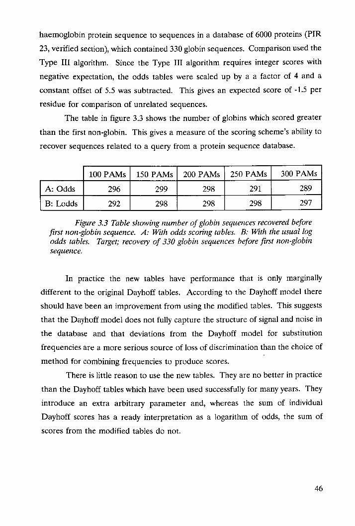
haemoglobin protein sequence to sequences in a database of 6000 proteins (PIR
23, verified section), which contained 330 globin sequences. Comparison used the
Type III algorithm. Since the Type III algorithm requires integer scores with
negative expectation, the odds tables were scaled up by a a factor of 4 and a
constant offset of 5.5 was subtracted. This gives an expected score of -1.5 per
residue for comparison of unrelated sequences.
The table in figure 3.3 shows the number of globins which scored greater
than the first non-globin. This gives a measure of the scoring scheme's ability to
recover sequences related to a query from a protein sequence database.
100 PAMs 150 PAMs 200 PAMs 250 PAMs 300 PAMs
Odds 296 299 298 291 289
Lodds 292 298 298 298 297
Figure 3.3 Table showing number of globin sequences recovered before first non-globin sequence. A: With odds scoring tables. B: With the usual log odds tables. Target; recovery of 330 globin sequences before first non-globin sequence.
In practice the new tables have performance that is only marginally
different to the original Dayhoff tables. According to the Dayhoff model there
should have been an improvement from using the modified tables. This suggests
that the Dayhoff model does not fully capture the structure of signal and noise in
the database and that deviations from the Dayhoff model for substitution
frequencies are a more serious source of loss of discrimination than the choice of
method for combining frequencies to produce scores.
There is little reason to use the new tables. They are no better in practice
than the Dayhoff tables which have been used successfully for many years. They
introduce an extra arbitrary parameter and, whereas the sum of individual
Dayhoff scores has a ready interpretation as a logarithm of odds, the sum of
scores from the modified tables do not.
46

Other amino acid similarity scoring tables
Many indices have been devised for comparing amino acids (Nakai et al.,
1988). These are based on measured chemical and physical properties. Scoring
schemes for scoring amino acid similarity based on differences of the indeces do
not take account of the mutational process. Such scoring schemes are rarely used
for protein database searching. Taking account of mutational change improves
detection of similarities arising from divergent evolution from a common ancestor.
Similarities between protein sequences suggestive of similar structure and hence
function will almost certainly be of this kind. One argument for using scoring
tables based on chemical and physical properties instead of the Dayhoff tables is
that potentially we might detect other functionally important sequence similarities
that have arisen by 'convergent evolution'.
With convergent evolution, the same enzymatic function is achieved by
evolution from very different ancestral sequences. Two proteins that have
achieved similar functions by convergent evolution may have similarities in the
three dimensional positioning of their interacting residues at the active sites with
this positioning of residues being achieved by radically different folding of the
proteins. Residues equivalent in the folded structures would then have markedly
different order and spacing in the linear protein sequences. The two classes of
serine protease, representatives being subtilisn and chymotrypsin provide an
example of this (Kraut, 1977). Both classes of protease have essentially the same
mechanism of action. Residues that are functionally equivalent can be identified.
In the linear sequences, these equivalent residues are not flanked by local regions
of sequence similarity. The kind of structural similarity the two classes of protease
show cannot be detected from the sequence data.
If convergent evolution cannot be detected by sequence comparison alone,
then it is correct to use a scoring scheme, such as Dayhoff's, based on divergent
evolution to score sequence similarity. Using such a scoring scheme can give a
sensitive method for finding weakly related sequences against a background of
noise.
47

Chapter 4: Rapid and Sensitive Database Searching
The sensitivity of the Type III NWS sequence comparison algorithm makes
it the method of choice for comparing pairs of proteins. The documentation for
the GCG sequence comparison software suite states:
"Bestfit [the local homology algorithm] is the most powerful algorithm we know for identifying the best region of similarity between two sequences whose relationship is unknown." (Devereux et al., 1989a)
Comparison of two proteins using the Type III algorithm produces an
alignment and a similarity score. The algorithm can be used for searching a
protein database to find if any sequences in the database are similar to a 'query'
sequence. Comparison of the query to each protein in the database produces a
list of alignments and similarity scores. This list is sorted by score and the high
scoring similarities printed out in order of rank, highest scoring first. As well as
printing the high scoring sequences' names and their scores for comparison to the
query, alignments of the regions which show similarity can be printed. The
alignments contain qualitative information whereas the scores are purely
quantitative.
Examination of the alignment may show a similarity is less convincing than
the score suggests. The similarity may be due to a section of unusual amino acid
composition in both query and database rather than to a conserved pattern. Such
a similarity may provide less evidence for functional relationship than more
heterologous matches of equal score do. This particular artifact of the scoring
scheme is a case of the assumption of 'independence of sites' implicit in any
amino acid scoring scheme, breaking down.
Because the similarity measure is imperfect, it is usual to present not just
results which are clearly signal but also some of the highest scoring results which
are likely to be noise. Amongst these, the biologist may spot an alignment with
E;]

a protein which for biological reasons is more significant than the score alone
suggests. A biologist may have greater interest in a similarity low down the list
than one high up. For example, if the query protein is differentially expressed in
males and females then the biologist may attach greater importance to matches
of the query to sex specific sequences from the database.
Sensitivity and selectivity
Two words, 'sensitivity' and 'selectivity' are used in some papers on
sequence comparison in describing the quality of the searching performed by an
algorithm. 'Sensitivity' is used to mean the ability to detect weak signals.
'Selectivity' is used for the ability to reject noise matches. In producing a list of
similarities sorted by score, selectivity can be improved at the expense of
sensitivity simply by printing fewer of the results of the search. 'Sensitivity' and
'selectivity' are thus different aspects of one quality, the ability of a sequence
similarity scoring scheme to distinguish between signal matches and noise level
matching.
Computational cost
In comparing a protein sequence against all sequences in a database many
thousands of pairwise comparisons are performed. There is a widespread belief
that the sensitive NWS pairwise method of comparison is too computationally
expensive to be used in this way on serial computers.
"The Needleman-Wunsch method is too slow for complete database searches to find sequences that are homologous to an input sequence."
"Use of the Needleman-Wunsch method to compare two sequences (of length 350 residues) took several minutes of machine time and more time is required for longer sequences." (Mount, 1988)
Consequently alternative solutions are sought. Various methods which are
acknowledged to be less sensitive are used instead (Pearson, 1990). This
approach is less than ideal. Ultimately the sensitivity of a method is more
important. One must consider the investment in time in experimental work to
49

determine the sequences. Lyall states:
"The real solution to this problem is to use a computer that is powerful enough to run the exhaustive algorithm as a matter of routine. As well as answering a real need, the use of such a machine may well catalyse the development of new methods for the understanding of biological sequences." (LyalI, 1988)
Lyall's work shows just how successful such an approach can be. He used
an ICL Distributed Array Processor (DAP) parallel computer which had 1024
simple processors. DAP computers are now manufactured and distributed by
Active Memory Technology Limited (AMT, Reading U.K.). Lyall developed a
fast parallel implementation, "Prosrch", of the Type III algorithm to run on the
DAP. In his doctoral thesis he presents six interesting and unexpected sequence
similarities found using "Prosrch".
Lyall also compared the performance of this software to software for
similar purposes running on various other machines. The use of the DAP turns
out to be cost effective particularly when compared to software on vector
supercomputers. The lesser cost effectiveness of such machines can largely be
attributed to the presence of special purpose hardware for floating point
calculations. This hardware adds considerably to the cost of the machines whilst
not materially contributing to speed of operation in this application.
Development of the early version of "Prosrch" which had a speed of
600,000 PMEs 1 has continued with improvements being made by Collins to
increase speed to 7,000,000 PMEs' and to facilitate investigations of the 'twilight
zone' between signal and noise matching (J.F. Collins, ICMB Edinburgh, personal
communication). Powerful hardware is clearly one solution to the problem of
combining speed with sensitivity. A disadvantage of parallel machines is that they
are not widely available.
50
Database reduction
One alternative way to increase speed is to reduce the size of the database
being searched. For example a database containing only representative members
of each sequence family could be searched. This inevitably reduces the ability to
detect weaker matches. Members of a family will show a range of values of
similarity score against any given query. The method works well when searching
with a sequence similar to the representative, less well when searching with a
sequence most similar to one of the more distant family members.
Rather than choosing a representative protein for each family, modified
sequences that attempt to capture the essential aspects of similarity shared by all
members of the family could be used. The use of such 'derived patterns' gives an
alternative method of database reduction.
Derived patterns
Using derived patterns for database reduction is possibly even less
satisfactory than choosing representative members, if the goal is to make new
discoveries through sequence comparison.
One of the sequence similarities reported by Lyall that was found using
"Prosrch" is indicative of the problem. A yolk amino acid storage protein (YP3)
in fruit fly, Drosophila melanogaster, was found to be similar to a lipase from the
liver of pig, Sus scrofa (Garbedian et al. 1987). A serine residue at the active site
is crucial to the lipase's lipid cleaving activity and is present in all members of the
lipase family. This residue would be part of a derived pattern for lipases. In YP3,
the residues in the corresponding position is glycine. This lead to a hypothesis
that YP3 is not a lipase, that it binds to but does not cleave a lipid analogue, a
precursor to a hormone called ecdysone. This hypothesis was confirmed by
experiment. The interpretation is that as YP3 is broken down to release its amino
acids to the growing larva, controlled quantities of hormone are released. Had
the computer search required matching of the active site serine residue the search
would not have detected the similarity.
(4E8/%
51

'Prosite
Databases of derived patterns are being actively developed. Though
caution is needed in their use, they are a valuable method for organising
information about sequences. The most comprehensive catalogue of derived
patterns so far developed is the 'Prosite' motif directory (Bairoch, 1989a). This
exists in both a printed and an electronic version. In the 'Prosite' directory
families of proteins are catalogued. For each family a 'motif pattern' is given.
The motif patterns of 'Prosite' represent 'key residues'. These key residues are
residues conserved or substituted for by similar amino acids in all examples of a
family. An example of a 'Prosite' motif for the Pentraxins, a family of serum and
plasma proteins some of which are expressed during acute phase response to
injury, is shown below:
Pentraxin family signature HXCX(S,T)W
The bracketed residues indicate alternative possibilities at one site. An
X indicate a site at which any residue is acceptable. The patterns are short,
simple and straightforward to interpret. They are intended to be diagnostic for
family membership.
The 'Prosite' motifs make searching for membership of families extremely
rapid. The database of patterns is much smaller than the sequence database.
Release 4 of 'Prosite' contains 198 protein motifs with an average of five residues
in each motif pattern. As well as the small size, the fact that 'Prosite' contains
highly conserved residues makes fast exact matching of patterns more acceptable
than it would be were the selected residues more variable.
Insensitivity of 'Prosite patterns
A criticism of the 'Prosite' directory is the insensitivity of most of the
patterns. With the protein family cytochrome c, members of the family shows
strong homology throughout their length, that is over a stretch of some 100 amino
acid residues. In the 'Prosite' directory, a motif pattern of 5 amino acids is chosen
52

near to a haem attachment site. Whilst this pattern may be superior to other
possible short patterns, the use of a short pattern means that much of the
information is discarded.
The loss of information arising from using short patterns affects detection
of new members of a family. Whilst careful choice of motif can make the pattern
diagnostic for family membership for all data available at the time the pattern was
chosen, the motifs will not necessarily be so successful on new examples not
available when the patterns were designed. This is indicated by the fact that the
patterns are changed to accommodate new data. A fission yeast cytochrome has
a leucine in place of a methionine that is conserved in all the other known
cytochrome c's. A change in the motif pattern for cytochrome c was necessary to
take account of this new special case and this is documented in 'Prosite'. For
smaller families the range of variation at sites is less well determined. For these
families there is therefore less confidence that the chosen motif pattern, diagnostic
for all current examples, will continue to discriminate well with new examples.
Measuring information content of 'Prosite' patterns
The shorter patterns match against unrelated proteins more readily than
longer patterns would. From a table of amino acid frequencies such as the one
in figure 1.2, it is straightforward to calculate the likelihood of matching random
sequence with any motif. One way to express this is as the information content
of the pattern measured in bits, that is, the Log to base 2 of the probability of
matching (Shannon & Weaver, 1949). The motif patterns for 'Prosite' functional
sites have a wide range of information content from 8.6 bits (cell attachment
sequence), to 49.3 bits (nuclear hormone receptors' DNA-binding region
signature). The former pattern would be expected to occur by chance every 28.6
= 300 residues, i.e. 7,700 times in a typical database. One would expect to search
200,000,000 databases to find the latter pattern by chance.
The problem of poor diagnosis by pattern has been explicitly recognised
in the directory for the 'leucine zipper motif (information content 14.2 bits,
expected 160 times in a single database search):
53

"As this is far from being a specific pattern you should be cautious in citing the presence of such pattern in a protein if it has not been shown to be a nuclear DNA-binding protein." (Bairoch 1989b)
The problem of low information content is a general one that arises from
having few residues in each pattern. It is not restricted to this one example.
There is a danger that features postulated by pattern homology come to be
treated as genuine. One feature (information content for 'Prosite' pattern, 16.8
bits) that is notorious for this is the 'zinc finger' (Frankel & Pabo, 1988). The
dangers would be more obvious were a clearer indication of the specificity of each
pattern, either as a probability of random matching or in terms of information
content, given for each motif.
Use of 'Prosite'
'Prosite' does not represent an acceptable alternative to rapid and sensitive
database searching such as is provided by "Prosrch". Its function is instead to
annotate a new protein sequence with suggestions of sites with already known and
characterised function. Its role is complementary to full sequence database
searches.
Approximate methods for sequence comparison
Since NWS algorithms are computationally expensive, to make searching
possible at reasonable speeds on serial machines, faster methods which are less
sensitive have been developed (Pearson, 1990). The most popular of these,
"FastP", compares 800 protein pairs per minute. These more rapid programs are
invariably based on exact matching of words.
IrFastpe two tier approach
To overcome some of the sensitivity drawbacks of word based matching
"FastP" uses a two stage process. The initial search, based on exactly matching
words, acts as a filter. This picks out proteins for a more sensitive method to
examine. The filter reduces the workload of the sensitive method to a
54

manageable level.
In "FastP's" two tier approach the first stage, the initial filtering, may
discard matches which would score highly under the more sensitive method. A
match that would be accepted in the more sensitive stage is not guaranteed to
pass through the coarser first stage and could be lost. In this sense the two stages
are not fully compatible.
The risk of missing a good score can be reduced by letting more results
pass through the filter to the second stage, that is by reducing the stringency of
the filter. There is no criterion though for how to set the stringency to guarantee
that all high scores will be found. For a discriminating comparison either a more
sensitive method must be used throughout, or a filter must be devised that cuts
down the workload but which is guaranteed to pass on all matches which would
be recognised as 'good' by a second stage.
"FastP's" second stage
The second more sensitive stage of "Fast?" performs an NWS-like
alignment to refine the score. This stage uses exactly matching words rather than
individual residue matches. As a result far fewer possible alignments need to be
considered. Additional speed benefits arise from using a dictionary just as they
did in the filtering stage. Even if filtering parameters are set to pass all proteins
to the more sensitive stage, the final scoring is still based on exactly matching
words.
A later development of "FastP" called "FastA", improves the second stage
by scoring words using Dayhoff scores in the more sensitive phase. In addition it
overcomes a major defect of "FastP", that "FastP's" first stage was a global rather
than a local algorithm. Previously, in longer sequences, a smaller region of good
matching could be obscured if there were insufficient word matches in it to be
significantly above average for sequence comparison of entire sequences.
The "FastP" algorithm is asserted to have running time that depends on the
sum, rather than the product, of the lengths of sequences compared (Wilbur &
Lipman, 1983). In fact, since the number of matching word pairs of a particular
fixed length is proportional to the product of sequence lengths, "FastP" has time
55

complexity 0(11 2). However, the "FastF' algorithm makes considerable savings in
comparison to the Type III algorithm, which is also 0(n2). The use of exact
matching words of length 2 leads to an approximately 200 fold reduction factor
in the work performed, whilst maintaining a useful level of sensitivity. This makes
the algorithm very suitable for rapid database searching and "FastP" is in
widespread use.
Theoretical advances in comparison algorithms
The DAP program indicates the importance of methods which are both
sensitive and rapid. Theoretical advances might lead to algorithms that perform
with the rapidity of "FastP" and the sensitivity of the NWS algorithm on serial
machines. Theoretical work on the NWS algorithms shows that theoretical speed
improvements to the algorithm are possible, in particular improvements that lead
to the 'four Russians' version of the algorithm (Masek & Paterson, 1983). This
algorithm works by first calculating a large number of 2 by 2, 3 by 3 or more
generally K by K alignment path matrices. These are combined in producing a
path matrix for the complete alignment. The algorithm takes time 0(112/Log n)
rather than the normal 0(n2)
Using 1 by 1 submatrices the algorithm is equivalent to the normal
implementation and there is no gain. With K = 2 precalculation of around 10 10
submatrices is required. This estimate is based on 20 amino acids, a 100 PAM
table and an indel penalty of 10. Storing these submatrices in main memo!)' is
impractical on all but the largest computers. For the method to give any gain at
all, retrieval from disk of part results would need to be faster than recalculation.
The authors of the paper on this method do not mention a practical
implementation of this algorithm.
The four Russians approach gives a theoretical gain which seems to be of
no practical use whatsoever for protein database searching. Log n grows slowly
with it, so it must be very large before we can hope for an appreciable gain. As
a minimum it must be large enough to compensate for the overheads in
precalculating the submatrices. In practice these overheads are colossal. Not only
is the time needed in calculating the submatrices large, the storage requirements
56

for the matrices are large too. There is an exponential increase in number of
submatrices with increase in submatrix size, alphabet size, mdcl penalty and range
of score in the scoring table. For protein database searching, using reasonable
parameters, the. four Russians method is impractical.
Concluding remarks
Speed and sensitivity are important in protein database searching.
Approaches to achieving these apparently conflicting goals have been taken by a
number of authors with varying degrees of success. These include database
reduction, use of word based methods, use of powerful computers and
fundamental changes to the algorithms for NWS string comparison. A fifth
approach, taken in this work, recognises the potential for improved serial
implementation of the Type III algorithm. This resulted in an extremely rapid
serial implementation. This is described in the next chapter. This algorithm is of
similar speed to "FastP", runs on a microcomputer and has the same sensitivity as
the DAP "Prosrch" algorithm.
57

Chapter 5: Techniques to Get More from Machines.
In the previous chapter we looked at various approaches to rapid and
sensitive database searching. Here we present a new approach that uses new
implementation techniques. These give a fifty fold speed improvement to the
serial Type III algorithm. The new implementation's importance is that it makes
the Type III algorithm run rapidly on widely available machines, that is on
personal microcomputers (PCs) such as those manufactured by International
Business Machines. In later chapters we discuss applications that were built
around this software.
As well as describing the new techniques used for rapid sequence
comparison, this chapter describes other implementation issues encountered in the
study. The chapter is divided into sections covering specific problems. Each
section starts with a statement of the problem, is followed by a description of the
methods used to tackle the problem and finishes with a discussion. The methods
sections concentrate on the principles behind the methods used. Further detail
of methods are contained in appendices where appropriate.
Type III comparison (Speed)
Problem:
A crucial problem with a standard implementation of the Type III
algorithm is its low execution speed. Apart from the use of parallel computers,
other techniques to improve speed make some compromise on the sensitivity of
searching in order to obtain their speed.
"The results of searches with FASTA compare favourably with results using NWS-based programs that are 100 times slower. FASTA is slightly less sensitive..." (Pearson, 1990)
RK

The problem tackled here is to find techniques that increase the speed of the
Type III searching on serial machines.
Methods:
A combination of techniques, rather than any one technique on its own,
were central to the speed improvements. Although each saving may appear to
have a marginal effect, the combined effect is significant. Savings in one part of
the algorithm only have a marked influence on the overall speed when other
inefficiencies are removed. Because the path matrix calculations involve
operations performed thousands of millions of times, apparently small savings can
have a large effect on the algorithm's running time.
The first step in improving performance uses the following observation:
Any two columns of the path matrix with the same sequence character at their
head will have the same one step diagonal scores. Production of a table of these
23 possible columns of scores gives a substantial saving in the number of indexing
operations the algorithm performs. Using this intermediate table, the number of
indexing operations in retrieving one step diagonal scores is halved. The row
index is used to directly access scores from one of the 23 columns in one indexing
operation, rather than first retrieving a sequence character (first indexing
operation), and then using the sequence character as an index into the amino acid
score table (second indexing operation).
The second optimisation is more complex. It rests on noticing that many
of the entries in the path matrix hold zero scores. This is true for over two thirds
of the entries. This arises because the scoring tables have a negative expectation.
The majority of paths score negatively and so have scores reset to zero at
each step.
Reorganisation of the order of operations is required. The Type III
algorithm is normally presented as in Chapter 2, in terms of how values at each
cell are computed. After re-expressing the algorithm in terms of how each cell
value influences its neighbours the fact that zero scores do not influence other cell
values can be properly exploited. Zero scores can then be processed rapidly. A
second saving arises from the new order of calculation. Provided that neither a
59

negative score nor a zero score influences other cell values, negative scores do not
need to be converted to zero.
For efficiency the software is written in assembly code. At this level of
expressing an algorithm, fetches of information from memory to processor and
storage of information from processor to memory are made explicitly. Deferred
assignment of values held in registers to variables held in memory is a technique
that can sometimes be used to reduce the number of times values in processor
registers are written out to memory. This optimisation technique normally relies
on a guaranteed pattern of memory reads and writes. The effect of a
conditionally executed statement can disrupt this, and does so in the Type III
algorithm. However, a new technique was developed to extend the method of
deferred assignment. This new technique, 'conditional deferred assignment' is
described in Appendix 3. It recaptures the ability to have a known history of
memory interactions and uses multiple versions of the code to do this.
The final important optimisation step is to reduce loop overheads for
processing one column. The determination of maximum score in a column which
could be done in a separate loop is instead performed in the main loop. Having
one loop instead of two halves the loop overheads. Moreover, the test for
maximum need take place only in the infrequently executed code that deals with
larger positive path scores. This subdivision of the algorithm into parts for
different levels of scoring arose from the previous two optimisations. The testing
of the loop counter is removed by using a rogue value (an impossibly high value)
to terminate the loop. Testing for the end of the loop only occurs where
maximum score may be being updated. This arrangement virtually eliminates loop
overheads.
Discussion:
The new implementation of the algorithm performs an average of 200
protein comparisons per minute, a speed of 300,000 PMEs 1 . A sensitive database
search can thus be performed in under an hour on inexpensive hardware. The
machine code algorithm has been built into a database searching program "Prowl",
written in Pascal for performing such searches.
ZC

The new implementation is the result of successive improvements to the
efficiency of an initial version. The idea for an optimisation often arose from
simpler optimisations. The rearrangement of the order of calculation, for
example, arose from combining two optimisations concerned with low scores.
How is it that the scope for dramatic improvements in speed in the serial
Type III algorithm has in the past been overlooked? One possible reason is the
practice of using asymptotic measures to measure performance. The
improvements described in the preceding section do not affect the asymptotic
measure. Asymptotic measures are useful precisely because they are a property
of the algorithm rather than the implementation. The example illustrates a
danger in relying too heavily on asymptotic measures when dealing with a practical
computational problem.
There are precedents for this. Theoretical advances in algorithms for
linear programming problems that resulted in an 0(n6) algorithm are not used in
practice (Osborne, 1985). The normal simplex algorithm with exponential time
worst case performance performs better in practice and is used instead.
The situation for Type III searching is more prosaic. The asymptotic order
does not distinguish between variants of an algorithm that differ in speed by a
constant factor. An emphasis on asymptotic orders may have lead software
developers to overlook the substantially greater efficiency possible in the
organisation of calculations in the standard algorithm.
Path reconstruction (Memory space)
Problem:
Generation of comparison scores rapidly is not enough. Alignments as well
as the alignment scores are needed. The pressure for rapid computation is not
intense since only a small fraction of the sequences compared need to be
presented to the user as alignments. Rapid computation here is not crucial. The
problem in implementing the reconstruction algorithm is limited RAM memory.
On a machine with a large memory it is feasible to store an entire path matrix in
main memory. From this the alignment can be reconstructed in steps as described
61

Uses of multiple alignments
Investigating mechanism.
Multiple alignments are useful in investigations of the functions of
individual residues in a protein. They show which residues are variable and which
conserved. Residues which are conserved in all the sequences are the most likely
to be crucial to the function. These conserved residues may be part of the active
site in an enzyme, or they may be vital to the three dimensional structure. Where
there is variation in a column of an alignment the kind of variation also gives
information. It can suggest the role played by an amino acid. Some columns of
multiple alignments, for example, contain only charged residues. The sign of the
charge, positive or negative, may vary. Such a site in a protein is likely to have
a different role to one for which all substitutions are charged residues of the same
sign. Information about variations can thus act as a guide for experimental work
to determine the function of individual residues.
The pattern of conservation of residues can give information about cysteine
residues. These residues may or may not participate in disulphide bridges with
partners elsewhere in the protein. No other residue type can fulfil this role. Loss
of a disulphide bridge would be expected to have a marked effect on the structure
and stability of a protein. If one sequence in a multiple alignment lacks a cysteine
at a particular site which is cysteine in the others, it suggests that the cysteine is
used for some purpose which other residues can fulfil and consequently is not part
of a disulphide bridge.
An example which shows how multiple alignments can draw attention to
structurally important residues is a particular glycine residue which is absolutely
conserved in all haemoglobins. Studies of three dimensional structures reveal the
explanation. The glycine occurs where two alpha helical structures, the B and E
helices cross (Stryer, 1981). No other residue is sufficiently small to fit in the
space available.
The information which multiple alignments contain is especially relevant
to methods for secondary structure prediction (Zvelebil et al., 1987). The
variation at sites shown by multiple alignments gives additional information about
72

structure not present in a single sequence. One example of this is that residues
that vary are more likely to be near the surface of a protein than in the core of
the protein (Perutz & Lehmann, 1968).
Searching
Computer searches can make use of information presented in a multiple
alignment about the range of variations at each site. Smith & Smith (1990),
suggest one method that could be implemented using a matrix that gives scores
for each amino acid at each site, a 'template matrix'. In the template matrix most
weight is attached to residues which are absolutely conserved. Template matrices
are computed from multiple alignments, typically by averaging scores for the
amino acids in a column. This takes into account the variability at a site and the
kind of variation. A template matrix represents a consensus about the patterns
shared by the sequences. If previously unknown members of a protein family
conform to the consensus pattern of conservation observed in the known
examples, then a databse search using template matching will give more
discriminating searching for new family members than comparison using any one
example from the family could (Taylor, 1986).
One advantage of using a family consensus pattern is that a single
comparison of a new sequence against a pattern can be used to check for family
membership. It is worth emphasising that this may be less sensitive than
comparing a sequence individually with each member of the family in turn. The
new sequence may be more similar to the member of the family most similar to
it than it is to the consensus pattern for the family. A mental picture for this is
to represent the sequences as points. The distance between the points represents
the degree of dissimilarity. A family of sequences will form a cluster. The pattern
for the family could be represented by a point that is at the centre of the cluster.
A new member to the family is, however, likely to be closer to some member of
the family than it is to this centre.
Motif patterns such as those of the 'Prosite' directory discussed in Chapter
4, are also derived from multiple alignments. They offer an alternative and less
sensitive method for defining patterns of conservation.
73

Sequence editors
For pairwise alignment, NWS algorithms are the accepted standard. The
situation is quite different for multiple sequence alignment. No method has yet
become universally accepted. It is not clear how best to extend a scoring scheme
that works well for pairwise alignment to score multiple sequence alignments. A
second problem is that the natural extensions of the NWS algorithms to score
columns of three or more residues, rather than scoring residue pairs, have very
high computational demands. To make improvements to existing multiple
sequence alignment algorithms involves addressing both purely computational
problems, and the problem of defining what good multiple sequence alignment is.
The latter requires some knowledge of patterns which actually occur in sequence
families.
To gain an understanding of patterns, many alignments for different protein
families must be examined. Moreover these alignments should be adjusted to
explore possibilities different to those suggested by computer alignment. Patterns
which computer analysis misses can only be characterised by manual examination
of sequences.
For closely related proteins, alignments can be examined and adjusted on
a text editor. For all but the simplest alignments this is time consuming. With a
text editor it is easy to delete sequence characters accidentally when removing
unwanted spaces from an alignment. There is a need for special purpose multiple
sequence editors.
There is a second reason why a multiple sequence editor is important for
development of new automatic methods of multiple sequence alignment. A
multiple sequence alignment editor can act as a front-end to a new alignment
method. It can take care of the loading and the formatting of sequences and the
display of results. This simplifies the testing of a new multiple alignment
algorithm.
The need for a multiple sequence editor is not specific to investigation of
improved algorithms for alignment. Until automatic methods produce entirely
satisfactory results manual adjustment of computer generated multiple sequence
alignments will continue to be important.
74

A number of multiple sequence alignment editors have been described in
the literature; "Lineup" (Devereux et al., 1984) "Homed" (Stockwell & Peterson,
1987), "Mase" (Faulkner & Jurka 1988), "Esee" (Cabot & Beckenback 1989) and
"Alma" (Thirup & Larsen 1990).
Sequence editor on the VAX
Initially work on multiple sequence alignment used the GCG "Lineup"
editor running on a VAX computer. With this editor alignments of the lipase /
yolk protein family discussed in Chapter 5, and of a family of citric acid cycle
proteins were explored.
Fortran source code for "Lineup" was available. "Lineup" was modified by
addition of new code to perform automatic multiple sequence alignment using a
new method. The new method performed all 112 n(,z +1) pairwise alignments of
11 sequences and recovered information about compatible parts of the alignments.
Where all alignments agreed, it aligned these residues, regions between being
divided into unaligned blocks. The new method proved unsatisfactory for all but
the most closely related families of sequences. It depended on low levels of
conflict between the pairwise alignments. This only occurred in the
straightforward cases, strongly related sequences or parts of sequences, that were
easy to align 'by eye'.
The VAX development environment and "Lineup" editor proved to be
unsatisfactory for this work. "Lineup" is the largest program in the GCG package
consisting of 10,000 lines of source code excluding subroutines shared by other
programs in the package, for example subroutines for reading sequence files. To
reduce compilation times, compilation was restricted to the new program section,
the bulk of the code being pre-compiled. Howevei, linking of the code was still
necessary for each change. This took a minimum of three minutes. This contrasts
with combined compilation and linking times of a few seconds for modular
software written in Turbo Pascal for the IBM PC. As well as having a
development environment that greatly facilitated program development, the PC
had a second advantage. The PC had the potential for an alignment editor with
a better user interface. For the VAX, updates to the screen had to be kept to a
75

minimum as the updates took place over a relatively slow serial line. The PC
permitted a much more responsive user interface as well as the use of colour.
The speed of response in particular was felt to be important for interactive
exploration of many different possible alignments.
Development work moved to the PC. To make this move a new multiple
sequence editor for the PC was written. This program was called "Medal" for
Multiple sequence EDitor and ALigner. The new editor could be more readily
modified to test out new ideas than could "Lineup".
"Medal" has a modular design. It makes use of the Turbo Pascal facility
to define software 'units' containing related subroutines and datastructures. This
modularity is important in development work. The automatic multiple alignment
routine of "Medal" is contained in a separate unit and could be replaced with an
alternative one without losing the interface features.
General editor interface features
Some of the interface features of "Medal" are relevant to general editor
design and not specific to Molecular Biology. They are not essential for the actual
task of sequence alignment editing. Features such as the 'help' facility could easily
have been omitted. One reason for developing a good interface to the editor was
to encourage use and criticism of the program by molecular biologists.
Computer interface design is itself an active field of research (Long &
Whitefield, 1989). Rather than performing a thorough study of interface design,
designs that worked well in other applications were adapted.
"Medal" has pop-up directory lists from which any individual file can be
selected. Pop-up menus are used in many PC programs. In "Medal" the pop-up
directory has an additional facility to allow selection of ordered sets of files. This
is needed for creation of a multiple alignment from a number of independent
sequence files. Pressing 'enter' selects the file currently indicated by a block
cursor. Each selected file is moved to the start of the pop-up menu and is
highlighted (figure 6.1). Files that have.been selected can be deselected in the
same manner. The whole set of selected files can then be accepted by another
key press.
76

Fiçure 6. 1: Pop-up directory for ,eIecting sequences IC tnükc a mLtl!iJ)le alignment. The file names in yellow are the selected sequences. The file currently open to selection is indicated by the purple block cursor.
I nil It 1jilf, rI iiif . Al4 flr I U I
Fiurc 0.2: "Medal 'S'' ac li/tv. The cuminand current/v elecied hi the cursor is described more fully in the top two thirds of the screen.
77

l,1.j. L__i—U ad LIps..14s ,'ta
sAlSflUUASILLXGNSX1. . If YIU I?SAUFTVUl3UGllSEftAkllS . Gill. UJAGUHY . FPflVIPS IAYTZflUAUGLTEflAUI .6 ISYCTA . TYPV AS MIRS .$c
T?VAU . GJRLSE1LFNNUUHLIYI IrTuursHrp IGTUGLT9!A 1111% IfllUiTTSTSyTpIflm
i?QUATVGYS!AIAHII) .GIETI$1TLTpJflAI , .UAAY!GG!UAIMALGLAKU. : LDLIFV?GUT?ThrS IATUGLTEQQAIU .69. UITSUL?LMUPMLIMItT?G V. IMMAGTIAA IMHTGG)AA. . . LDLTAIIPAUUFTDPQUATUG?S!AEAHH) .6 ItT). SiTLTLMlU?iAL*pflhi I. UAAAA6TRA*IPIIITGGDAA. . . LNLTAMPAUU? TbTQUATUG?SEAEAHHI .6 tIC?). SiTLTLUpMyfl1
V
p jut. I$EDfI)Q IU IGAHL ISISEAIEI. 1$HrKF6IsTKELICQHI FAT jtAAsi IAHIIL............... GIITILI9KE .SHIV I 166* IUGT)SGGELLGE I IEPIGC)A!) IJAH jLHES6LMtVFEGS1T)'2llu* ILIL(UGSEE. x IUIGINGIGFGVIPEIILQGF KIIGATICK)F III? I*AEEFUTflI...............
11.KLU.IEEGSGILI 6 UIUCAISKU . KUU 6 IHIIQGLGCDEIILQGFA'
V?.JLU.UIIAQTQICLI GAHI f1.NLU.I!EGSHRLI Gj§PA
T USO T FI.KLU.UEEGSGBLI 6
ft-hip fl-kr F3-I..ck 14-k1.ct VS-kt flh-CuuO
alteft h_J-I• Liao hL..Jk 1.1 UpsisMs esitass
m3A341)SHUUASHLLKGNSØ. . JEYPU I?SAUV TUPKIIASUGISSZE!AINS .61I. HIGHIIE .GSHMAE . UIAGICKNY. F)PKUI?SIAYTEP!U*HUGLTEKEAIU .615flTA . TV? ASGIALAS .KHI T?UMM* . GJJLSULFMMX?DEHL)?SH I?TUUFSHP? IGTUGLTEPQAMvGlwmvxnrymitwiTww T?UA!M . GUL*HILVEYKEDSXLDYMSI I?TWFSHP? I6TUGLT!)EA1HI%
.................... )PQUATUGYSEAE*HH) GIST). S1TLTLPW?AI6 V .IMAYEGGIIMIWIALGLAXIX. . IDLRFUPGUTFT1IPS IATUGLT!QQAKEK .6?). UICTSUL?L)J?$LJm V .TIaA1NHTGGDA*. . . LDLTANP*UUFTDPQUATUGYS!AEAHH) .61!?) -SITLILUMIALMnTIG V. UMAAGTMA IMHTGGDM. . . LMLTAH?AUUFTD?QUATUG?SEAEAHH) .6 Ill?). SITLTL)IIVP.y.T
V
A,.IUL. I)!IHDQIUIGAHLISNEADELINHFAT.IIi?GISTXELKQIIIFAYIIAAS)IAImL ..............
II .KIUCUGSE! . XIV 161116 IGFGIIDEMLQGFAU. GATICKIF 111 AAEUVTIIJ.............. STItLI1JICE . SHIU 1166* IUGTPIGGELLGE ICM9 IlAHILHE3VGLAA!UflG3IflUIW1
V?.KLU.I*IAQTQXLI GA A. ?GLTI!DLTI
UN. UIUCMKEE . KUI]GIHHQGLGCDEhLQGFAU. MKA)T)l 7I.ZLU.IEEGSGRLI GJU T. IRtIINTlJLAl
FIJLU.IUGSHRLI 6 T. IR$IMT1LAI ?I.XLU.U!EGSGKLI 6 T. 1111111? LA]
a
?
XM6ATKA$9I 1RH8PITILA1
QF6LTIEDLTI IRIIEMT LA] IRNRfl.T LA]
SSULUTIJ............... IIUEGLKLAAQTFTDUKQLSCCMMEGLKLAALT9UUSIL3CMHUEGLILAAQTThKWKQLSCCM
SSULVTLI..............
0jMut6uLA*QT1T05cd1 IIAEGLKL*ALTTIK$SIL3cCI MU!GLKL*AQTFIII$IIL3tU
I ,MU!6LILAA4T?IIXMLScC1

In "Medal" menus of commands and the on line explanatory 'help'
information are combined in one system. When selecting commands the lower
third of the screen contains a menu of commands. The command currently
selected off the menu has help information about it displayed in the top two thirds
of the screen (figure 6.2).
"Medal" uses an initialisation file which records path names. These paths
indicate directories in which sequence and alignment files are stored and the name
of the alignment most recently worked on. When "Medal" is invoked the most
recent alignment is fetched into memory so that alignment editing can resume
where it was last left off.
Platforms and interfaces
The editor interface design illustrates the influence of the platform. On
a machine with a slow transfer between screen and memory, update of help
information as each menu command was selected would have lead to a very slow
response and would have been impractical. Multiple sequence editors on other
machines follow interface practices for those machines. The "Lineup" editor uses
interface features from the VAX/VMS editor "EDT" such as the use of ctrl Z to
end screen based input. The Unix "Mase" sequence editor uses binding of keys
to longer commands similar to that found in the Unix editor "emacs".
Sequence editing features
Other features of "Medal" were designed specifically to assist multiple
sequence alignment editing. Normally in "Medal" all sequence characters are
shown in grey. Pressing a key on the keyboard causes all occurrences of the
character to be displayed in a preselected colour. Residues which are
conservative substitutions use the same colour. Pressing the key again causes all
occurrences of that character to revert to grey. This feature helps in locating by
eye patterns of similar residues.
"Medal" allows regions of the sequence to be delimited. A vertical bar in
an alignment prevents changes made on one side of the bar from affecting
79

in Chapter 2. Storage for the full path matrix is not necessary if only scores are
required. In the searching phase only two columns at a time are needed. For
reconstructing the alignment, the path matrix size can be a problem even on
mainframe machines. In the GCG implementation path matrices are limited to
1,000,000 elements. This is sufficient for two sequences of length 1000. On
microcomputers the memory problem is more severe.
The "Prosrch" program described in Chapter 4 has one solution to this
problem. With the "Prosrch" program both endpoints of any alignment path are
obtained in the searching pass. Whilst this adds a substantial overhead to the
searching time it simplifies the post processing'. When both endpoint positions
for a Type III alignment are available reconstruction of alignment is equivalent
to a Type I alignment. For Type I alignments this reconstruction can be done in
a space efficient manner using 'divide and conquer' techniques (Hirschberg, 1975).
These require recalculation of some of the path matrix entries.
"Prosrch" in fact uses a more sophisticated hierarchical approach. It tries
successively more complex algorithms in turn. This sequence is optimised for
alignments with few gaps (J.F. Collins, ICMB Edinburgh, personal
communication) and is extremely efficient in these cases.
The new serial Type III implementation described in this chapter finds the
endpoint but does not find the starting point of an alignment. However, as each
column of the path matrix is calculated, the software finds the score and location
of the best path ending in the column. These values are used in finding the score
for the overall best path and the location of its endpoint. The requirement is for
an efficient way to reconstruct the alignment given only this information for each
column.
1To do this, each path matrix element must carry start coordinates of a path in addition to a score.
62

Method:
The strategy employed to do this, like the divide and conquer approach,
uses recalculation to reduce memory requirements. The strategy is not
guaranteed to use as few recalculations but its behaviour is good in practice. The
method uses the stored values for the best path ending in each column to reduce
the likelihood of needing recalculation. Many of the recorded locations are
actually on the best path. The reconstruction is particularly rapid where this is the
case. Reconstruction proceeds as described in Chapter 1 except that only ten
columns of the path matrix are available at a time. Moreover the values present
may be lower than they should be. Consequently the retrace procedure may be
unable to continue before having retraced the full path. In that case, path matrix
recalculation is started from fifteen columns prior and generates the ten columns
immediately before the column of the current cell. This recalculation starts by
setting the first of the fifteen column's scores to zero, whereas in fact some of the
values should normally be positive. This is the reason for some values being lower
than they should be. The recorded best endpoints in a column are put in place
after each column is calculated. This step ensures that if any one of the fifteen
recorded best endpoints prior to the current cell is actually used on the best path,
then the path being reconstructed can be continued. This is usually the case for
high scoring alignments. The approach also works if the path started within 15
steps of the cell currently reached. This tends to be the case for short low scoring
alignments. If, however, this stage also fails to extend the path, recalculation can
be started from the start of the sequence and will yield correct scores, rather than
reduced scores, for the immediately prior ten columns.
Discussion:
This strategy works well in practice. It also is simpler to program than the
'divide and conquer' technique. This results in a shorter program. The divide and
conquer method needs to change the direction in which sections of the path
matrix are calculated. The new method does not. It uses the same score
calculation code for reconstruction as used in the search. Since this code has been
heavily optimised, reconstruction of alignments is rapid. The method also extends
63

gracefully if more memory is available. Storage for more columns of the matrix
leads to lower likelihoods of repeated recalculation.
Database compression (Disk space)
Problem:
A second problem with microcomputers is limited disk space. One
investigation concerned methods to compress the sequence database. The method
developed has an exceptionally rapid decompression algorithm.
Compression technique:
Standard compression algorithms, such as the Lempel-Ziv algorithm, work
by identifying short patterns which occur many times and choosing compact
representations for these patterns (Welch, 1984). The new method recognized a
common kind of repetition that occurs in sequence databases - longer sequences
of characters that are repeated just a few times.
Ovvvvvvv lnnnaaaa aaaaaaaa llllaaaa aaaaaaaa rrrrrrrr
vvvvvvvv nnn
aaaa aaaaaaaa rrrrrrrr
Single character. Repeated run of length 3-9. Repeated run of length up to 256.
Character value (7 bits). Run length in range 3-9,
represented by 000 to 110. Offset to previous occurrence of run. Run length in range 0-255.
Figure 5.1: Coding scheme used to represent repeated runs. Above: The three forms in which data is represented in the compressed file in terms of bit fields. Below: Interpretation of the bit fields.
A compressed run is represented by a word (two bytes) with the top bit set.
The lower twelve bits represent the relative location of the run. The remaining
3 bits represent the length of the run. 000 to 110 represent runs of length 3 to
64

9. Longer runs are represented by 111 and the byte after the word gives the
actual length up to 255 characters.
The standard compression methods would be unable to exploit such longer
patterns nearly so well. The Lempel-Ziv compression algorithm, for example,
needs to 'learn' each shorter run in the long repeated run before it can learn the
long run and represent it with maximum efficiency. The effect of this is that to
'learn' a longer run, the Lempel-Ziv algorithm must see it at least as many times
as its length. In the database, many of the long repeated patterns occur only a
few times. With the new method a long run only needs to be seen once for future
occurrences to be compressed.
Using the algorithm 2.5Mb of the PIR 23 database was compressed to
1.2Mb. Later, commercial software for compression, the program "PKZip"
(PKWare Inc, WI 53217, U.S.A.), was available. This algorithm achieves the same
compression factor, though it is not clear what compression algorithm it uses.
Discussion:
For machines for which disk performance is a severe problem, compression
gives an effective increase to the capacity of the disk. It also gives an effective
increase to the speed of disk read access since decompression is more rapid than
disk to memory transfer. Compression software improves the effective
performance of the disks. In practice the method was only used to reduce the
number of disks needed for data redistribution.
Data compression may become more important as the 'human genome
project', an international project to sequence the 3x10 9 bases of the human
genome develops (Gordon, 1988). When distributing data to a large number of
users, the potential savings from reducing media costs could conceivably be
significant. The increased speed of access is unlikely to be a critical factor as for
sensitive searching on low cost hardware the rate limiting step is the actual
comparison.
The technique is particularly attractive for representing slight variants of
a gene. At the moment there is an inconsistent policy over representation of
sequence variants in the database. Sometimes a variant sequence is given a new
65

sequence entry. At other times it is recorded in feature tables that give
alternatives at particular sites. Variants so represented are not searched by
current software. Using the kind of compression suggested here, full entries could
be made for these variants with minimal media costs.
Tripeptide matching (Speed).
Problem:
For part of the study a very fast approximate sequence comparison routine
was required (Chapter 7). A coarse method was acceptable as only the very
strongest similarities needed to be found.
Method:
The coarse comparisons were made using a program to count exactly
matching tripeptide words shared by pairs of proteins. The program took each
protein in turn and used it as a query against the database. To make the counting
of shared tripeptides rapid a tripeptide index for the query sequence was used.
To increase the efficiency of disk access, software to cache data from the database
was written.
A near eight fold speed improvement on this basic method was
subsequently achieved by searching with eight query proteins simultaneously. This
reduced the disk overheads by a factor of eight and, by splitting integer scores into
fields, one addition operation was made to serve the update of all eight proteins
scores. Overflow of the fields was avoided by periodically using the fields to
update scores with a wider range.
With these enhancements the comparison program could perform
32,000,000 coarse tripeptide based pairwise sequence comparisons over a
weekend.

Discussion:
Even more rapid techniques are possible using sorting of subsequences
from the database. Here a technique that compared each protein pair in turn was
required partly to test the software framework for total database searching. A
relatively simple method was found to be satisfactory.
Annotation browser (Portability)
Problem:
A screen based application for examining lists of results from database
searches was written. The program provided a rapid method for cross referencing
between search results and sequence annotation databases. The first version was
written for emas, a mainframe computer which had ample disk memory and which
held the sequence annotation files. The program, which was called "Xref', was
initially written in IMP, the language of choice on the emas computer. Later the
software was required for other machines. Since the program was not
computationally intensive, portability seemed to be an important design goal for
the rewrite.
Methods:
"Xref' was rewritten in Turbo Pascal for the IBM microcomputer with the
intention of porting it onto a Unix machine. This was initially thought to be a
good development route. As well as producing a version of the software for the
microcomputer, it gave the opportunity to use the excellent development
environment of Turbo Pascal in rewriting the code.
Documentation on the Unix Pascal that was available for the Unix machine
turned out to be insufficient. There was insufficient information about file
mapping, control of the intermediate PAD I/O computers and access to terminal
characteristics. In addition the Unix Pascal compiler did not support some of the
Turbo Pascal type casting operations that were essential to the program's
operation. Just as IMP is the best supported language on the emas computer, so
C is the preferred language for Unix machines. More facilities were readily
67

available in - C and C seemed to offer possibilities for a more portable
implementation. The program was therefore rewritten in C using the Unix
terminal independent screen and cursor control subroutines 'Curses' since one
factor which reduces portability is having software depend on specific hardware
features. The 'Curses' routines are aptly named. Using the routines an addition
of a single line at the top of the screen resulted in the whole screen being redrawn
to achieve reverse scrolling. This was slow and made the program useless as an
interactive tool. The compromise solution adopted avoided the 'Curses' software
and provided direct cursor control sequences for VT100 compatible machines
(Wyse, 1984). These sequences gave correct scrolling action for Sun workstations,
VT240 and Wyse 75 terminals and microcomputer terminal emulators. In practice
this restriction in terminal type did not cause problems.
Discussion:
The observation from experience with "Xref' was that translation of
software to different languages provided a rapid route to porting software
between different machines. Overcoming the portability problems of the Pascal
version would certainly have taken longer than rewriting in 'C'. Although the
program was not compute intensive it seemed to require a compromise in
portability. This was a result of the need for fast screen I/O.
Optimisation to "Prosrch"
Problem:
The PC program demonstrates the possibility of sensitive database
searching at reasonable speed using the Type III algorithm on a microcomputer.
The software can be used to do a comprehensive comparison of every pair of
sequences in the database (Chapter 7). However this takes several weeks of
computer time. A natural question to ask is: "Can the same techniques also be
applied to accelerate database searching on a parallel computer?". If so,
comprehensive sensitive pairwise comparisons of databases could be made on a
routine basis.
Methods:
To investigate the possible optimisations of a parallel program, source code
for the 'Prosrch" program was examined and modified in the time critical sections.
These modifications illustrate the potential for optimisation but to fully evaluate
them would require substantial changes elsewhere in the software.
Experience from optimising the serial implementation drew attention to
aspects of the calculation where savings could be made. The programming
techniques to do this were different; none of the techniques discussed for the
serial code apply. The details of the methods are peculiar to the parallel
computer's architecture and the 'Prosrch" program and are described in Appendix
4.
Discussion:
The serial techniques used to achieve speed on the microcomputer are not
applicable to the parallel computer. The serial techniques rely on case analysis
to make processing more rapid. On the parallel machine many cells are
processed at once. These must be processed with the same set of instructions.
On the parallel machine separate processing of different cases slows down
operations. Multiple cases take the sum of the time for the different cases, rather
than a weighted average of the times. Radically different optimisation techniques
need to be used.
The study provided an alternative set of optimisations suitable for the
parallel machine. More important than a potential for an estimated eight fold
speed improvement was a dramatic reduction in code size arising from the
optimisation method. This should aid maintainability and future modification of
the software for other uses. The techniques described in Appendix 4 would also
be appropriate for efficient implementation of the more computationally
expensive string comparison algorithms of Chapter 9.

Concluding remarks
Practical considerations draw attention to computational problems that are
different in kind to purely theoretical studies. In the main these can be tackled
by adapting and applying combinations of standard computing techniques. For
practical systems, it is not so much individual techniques as combinations of
techniques that matter. This is so both at the level of individual subroutines, such
as the new Type III subroutine, and at the level of applications programs.
70

Chapter 6: Multiple Sequence Alignment
Multiple sequence alignments show in a compact format relationships
between several protein sequences. They differ from pairwise alignments by
having extra rows for additional related sequences in a family. The presentation
of information is more condensed than if a set of pairwise alignments were shown.
Strong patterns present in all sequences are readily distinguished from patterns
present in only some sequences. These patterns would be harder to see by
examining pairwise alignments. An example of a multiple alignment is shown
below:
++++++ + ++. + +.+ .- + + + + +++ ++++ A30007 : APKIFGGEIKTHILLFLPKSVSDYDGKLSNLKKAADGFKGK ILFVFIDSDHTDNQR A26289 :APKIFGGEIKTHILLFLPKSVSDYEGKLSNFKKAAESFKGK ILFIFIDSDHTDP4QR ISMS :APKIFGGEIKTHILLFLPKSVSDYDGKLSNFICJ(AAEGFKGK ILFIFIDSDHTDNQR R3EC2 :KPRIFGARNKVHIIN LEKTVPMFNEALAELNKIA SRKGK ILFVGTKRAASEAVK R3NT2 :APYISAKRKGIHITN LTRTARFLSEA CDLVFDAASR GKQFLIVGTKNKAADSVE R3LV2 :APYIFTERKc3IHIIN LTQTARFLSEA CDLVANASS KGKQFLIVGTKYQAADLIE
Identities '+' and conservative substitutions '.' are marked where four or
more of the residues are identical or conservative substitutions.
The top three sequences are strongly related to each other, so too are the
lower three. The relationship between the two families is less certain, the
similarity between sequences R3EC2 and A30007 providing most evidence for
there being a valid link. This particular alignment was produce to help
investigation of a hypothesised link between protein disulphide isomerases, top
three sequences, and ribosomal sequences, lower three sequences (see Chapter
8). Multiple alignments present more detailed information about the
interrelationships between sequences than a pairwise alignment can. Individual
columns of a multiple alignment show the range of variation at a site, assuming
that is, that the multiple alignment correctly aligns residues that are in structurally
equivalent positions.
71

residues on the other side. This feature is also present in "Mase" and "Esee".
The editor "Alma" allows groups of sequences to be locked together.
Insertions or deletions in any one of these grouped sequences affects all sequences
in the group. In "Medal" locking together is done on a per residue basis. Such
residues are shown with a coloured background. Residues which are locked
together stay aligned whatever other changes are made. Residues which are
locked together move together whenever any shift, insertion or deletion moves
one of them. This system makes it possible for the sequences locked together to
vary from column to column. This approach is more general than whole sequence
locking. Photos in figures 6.3 and 6.4 shows residue locks in action. The lock on
residues can be set and removed easily by a single keypress. Also an automatic
scan can be made that puts in locks for all currently aligned residues of similar
type. Locks are also placed after automatic alignment.
"Mase" and "Homed" have more limited whole sequence locking than
"Alma". They are restricted to locking together groups that consist of all but one
of the sequences.
Assessment of editor features
The editor part of "Medal" demonstrates the advantages of using
computers of the PC kind rather than a mainframe for multiple sequence editing
work. In many ways the advantages parallel those of using a PC word processor
over a mainframe text editor, a faster screen update leading to more information
on the screen at one time and user friendly help and menu facilities.
Additionally the "Medal" editor introduces a new concepts to multiple
sequence editing; the locking together of sequences on a per-residue basis. The
features in "Medal" were largely influenced by use of the program in creating and
modifying multiple alignments. Using per-residue locks on their own was found
to be not entirely satisfactory as for larger alignments changes can involve setting
and resetting many such locks.
One option in "Medal" combined automatic placement and removal of bars
at the boundaries of regions of sequence conservation with locking together of the
similar sequences over the region of conservation. This was found to be confusing

to other users of the software. For the kinds of editing for which this option was
designed an alternative would be more useful. This would give the user
temporary locking together of any subset of sequences over a region delimited by
the bars. Existing residue loëks would still be active. Were there time to do so,
this alternative option would be added in place of the present option.
Sizes
Of the editors considered, "Medal" has the smallest capacity for sequences.
Max. number of
sequences
Max. sequence
length
"Lineup" 31 100,000+
"Homed" 50 10,240
"Mase" 100 10,000
"Esee" 21* 18,000*
"Alma" 300 60,000
"Medal" 21* 6,000*
Figure 61: Sequence capacities of various multiple sequence alignment editors. Figures marked * are for programs on microcomputers. For microcomputer programs the maximum size and maximum number of sequences are 1101 available simultaneously.
Additional work would be needed to raise the number of sequences and
increase the maximum sequence length. Data compression techniques, as
described in Chapter 5, could be one way to achieve this. The alternative is to
make greater use of disk memory. Much larger datasets could be accommodated
by holding parts of the alignment not currently being displayed in disk memory.
Space could also be saved by making the automatic alignment process, currently
part of the "Medal" program, into a separate program.

Automatic alignment methods
Ideally an algorithm for automatic multiple alignment should find patterns
which do not show up when only pairs of sequences are compared. One approach
to this is a multidimensional extension of the Type I algorithm (Murata et al.
1985). Instead of a two dimensional path matrix, a K dimensional array, where
K is the number of sequences being aligned, is used. Each additional sequence
of length three hundred increases the workload three hundred fold. Whilst cutting
corners in the match matrix, that is calculating only elements near the main
diagonal, dramatically improves this situation, it brings with it a risk of missing
similarities when large insertions or deletions are required. Because of large
memory and time requirements, this direct approach has been limited to three
sequences.
Subsequent to Murata et al. 's work, a more sophisticated method for
restricting the volume explored in the multidimensional path matrix has been
developed (Lipman et al. 1989). The method uses an alternative formulation of
matching in terms of difference scores rather than similarity scores. The method
extends the multidimensional method to up to six sequences. Unlike conventional
corner cutting,the alignments this method finds are guaranteed to be optimally
scoring by the scoring scheme.
Close examination of the method suggests that the computational costs
grow very rapidly with increase in sequence dissimilarity, even where this is
confined to short local regions. Thus, the method is applicable to up to six
sequences only when the sequences have very high levels of similarity.
A problem which is noted in the paper is that the scoring strategy needs
adjustment where one subfamily is heavily represented in the set, otherwise the
alignment is determined by these sequences, being then an alignment to the
consensus for this subfamily. This adjustment involves a manual intervention to
identify clustering of related sequences.

Using exact matching
Some algorithms overcome the problem of computational demands by
using exactly matching words (Sobel & Martinez, 1986; Bains, 1986; Santibanez
& Rhode, 1987). These algorithms can be seen as multidimensional extensions
of the Wilbur & Lipman (1983) approach. These word based alignment methods
have the same advantages as the word based pairwise methods - simplicity and
ease of calculation. The methods suffer from the same problems as the pairwise
exact word based methods. That is, lack of sensitivity over amino acids of similar
properties, inability to cope with single mismatches in a region of good matching
and inability to deal with insertions.
A promising variant of the exact matching word methods removes the
restriction that the amino acids be contiguous (Roberts, 1990). The variant, as
currently implemented, only detects the interrupted similarities, the multiple
alignment being performed manually. Allowing broken similarities overcomes the
problem of single mismatching residues ruining an otherwise matching word and
preventing its detection. This idea is examined again in the addendum in the
context of database searching.
Alignment refinement
A technique used as an additional stage in a number of multiple alignment
strategies is called refinement (Bains, 1986; Barton & Sternberg, 1987; Hennecke,
1989). After the initial multiple alignment has been made, individual sequences
are removed one at a time and realigned against the remaining sequences. The
process stops after a preset number of cycles or when no further improvement in
alignment score is achieved. The technique will not correct very poorly aligned
sequences but can fix 'glitches' where one sequence is obviously Out of alignment
relative to the rest. A modified form of refinement, claimed to have some
advantages over the simpler form, removes and realigns groups of sequences
(Subbiah & Harrison, 1989).
Refinement is popular partly because it is a simple addition to a program
that already performs alignment of sequences to aligned sequences. A
disadvantage of refinement is that realignment is performed against a consensus,
RE

so the criticisms of comparisons using consensus given earlier in this chapter
apply. Refinement, as its name suggests, can improve patterns already detected
by the initial method, but it is unlikely to detect patterns that the initial method
does not find. If a particular shared pattern is not evident from the consensus,
for example if the shared pattern is found in only two of the sequences,
refinement does not help. If the initial method finds such pattern, refinement is
likely to lose the pattern again unless the weaker pattern is bounded by strongly
conserved patterns that do show in the consensus. Refinement was not used in
the alignment algorithm of "Medal".
Multiple alignment based on pairwise alignment
One of the most straightforward multiple alignment methods is based on
pairwise alignments. The method is due to Taylor. He compared results of this
method to those of multidimensional extensions of the NWS algorithms as follows:
"Reasonable multiple sequence alignment can be achieved by a simple method. The results are equivalent to those obtained using a complex algorithm that considers the sequences simultaneously during alignment." (Taylor, 1987b)
Taylor built his multiple alignment using selected pairwise alignments. The
selection process required only a few pairwise comparisons. The method
considered addition of a new sequence to a multiple alignment of a few sequences
by pairing either to the first or last sequence. Results of this approach depend
on the order in which sequences are presented to the algorithm. This strategy
seems most appropriate for cases where the sequences represent various
intermediates between two extremes and are presented to the algorithm in an
order that reflects this.
The approach used by "Medal" adds one sequence at a time to a multiple
alignment, each time adding the new sequence most closely related to any
sequences in the alignment and aligning on this pair. This approach seems
appropriate to more arbitrary relationships between sequences than Taylor's and
includes Taylor's pattern of relationships as a special case. Moreover this
approach makes the alignment essentially independent of the order in which
sequences are presented to the algorithm.
Consensus alignment
Closely related techniques to "Medal's" are used in two other methods of
multiple alignment (Barton & Sternberg, 1987; Higgins & Sharp, 1989). Both
these methods perform all pairwise comparisons of the sequences to establish the
order of alignment. This frees the algorithms from dependence on the order in
which sequences are presented to them. For reasons of speed the programs use
the Wilbur-Lipman pairwise approach to perform all comparisons. The Type I
algorithm is then used in actual alignment.
The program of Barton and Sternberg differs from "Medal" in aligning each
new sequence to a consensus for the sequences aligned so far. This may give
better results if the sequence being .added is more similar to the consensus than
it is to any of the sequences in the alignment. This consensus strategy for forming
multiple alignments is inappropriate where the sequences show differing degrees
of pairwise similarity. In these cases the 'average sequence' is likely to be much
less similar to a given sequence than the most similar one of a set. This situation
frequently arises in practice. Sequences being aligned are often obtained from
closely and from more distantly related organisms.
Higgins and Sharp's "Clustal" program also uses consensuses. It
progressively aligns initially separated subfamilies of sequences. It combines
alignments by aligning pairs of consensus patterns. The problems of consensus
sequence alignment are less in this case. Because of the order in which
alignments are made, most patterns present only in subfamilies can be found
before the subfamilies are combined. In particular, anomalous patterns present
in just two of the sequences can be found. Anomalous shared patterns seen in
examining alignment by hand were nearly always present within subfamily groups.
Consequently "Medal" and "Clustal" should have very similar behaviour in most
cases. In exceptional cases such as the multiple alignment at the start of this
chapter, the link between the families is clearest from one pair of sequences.
Only in such cases would "Medal's" approach be expected to give superior results.

Equally there will be special cases where a clearer picture of similarity arises from
"Clustal's" approach.
Examining the different methods, we see that similar principles underlie
several different approaches. "Medal's" method can be seen as combining specific
elements of Taylor's and Barton and Sternberg's techniques to give similar
advantages to the "Clustal" method of Higgins and Sharp. In fact the relationship
of "Medal's" algorithm to "Clustal's" is closer than initially appears. In "Medal",
introducing sequences one sequence at a time is an algorithmic convenience. The
alignment "Medal" produces would be unchanged were it instead produced by
combining subfamily alignments basing alignment of these alignments on the most
similar pair of sequences in the two subfamilies.
Use of the Type III method in "Medal"
One motivation for developing "Medal" was to test the utility of the new
Type III software in practice. To perform the comparisons for clustering rapidly,
"Clustal" uses an approximate word based method. "Medal" is able to use the full
Type III algorithm, and performs the calculations faster as a result of the
optimisations to the implementation. The advantages of this in practice are slight.
The reason for performing these comparisons at all is to distinguish subfamilies
from each other. For this purpose, an approximate comparison method is as
satisfactory as the more extensive method.
In performing the pairwise alignments for the multiple alignment, "Medal's"
Type III alignment has some advantages over the Type I alignment used in other
programs. For closely related sequences the Type III 'best local homology
algorithm' aligns whole sequences and there is little difference between using Type
I and Type III alignment. For strongly and for less strongly related sequences, the
Type I algorithm forces alignment from end to end. Improvements in the
matching in unrelated regions may take precedence over the alignment of related
regions. In particular, an unmodified Type I alignment incurs penalties for
unmatched residues at ends of sequences and attempts to make the starts and
ends of sequences correspond. This problem has been addressed by modification
of the Type I algorithm to suppress penalties for the gaps at the ends of

sequences (Devereux et aL, 1989b). This modification allows one sequence to
terminate before the other without incurring a penalty. The local algorithm copes
with this problem without any modification. For Type III alignment, unmatched
residues at the ends of sequences lie outside the local region of alignment and
incur no penalty. As well as the case where one sequence is a truncated version
of the other, Type III alignment can also handle sequences that differ at their
extremities, a case which the modified Type I algorithm does not handle well.
Experience of multiple alignments made by hand indicates greater variability in
terminal sequences, so the ability of Type III alignment to handle this case is
important.
Recursive local alignment
A disadvantage in using the unmodified local method is that only one local
matching region will be found even if there are several. Additional local matching
regions are of interest to the biologist. Those regions compatible with regions
already found could be used to make a more complete alignment of the two
sequences.
The additional regions of similarity can be found by reanalysing the parts
of the sequence not included in the strongest local alignment. A recursive
sequence alignment method was developed following this principle. It was used
in "Medal" in place of the simpler Type III algorithm. The procedure finds the
best local region between two sequences, aligns these parts of the sequences and
then aligns the initial and terminal unaligned regions of the two sequences by
calling itself recursively. The recursion stops when the alignment score for two
sequence segments drops below a preset threshold chosen to correspond to
insignificant alignment, the value 70 being found suitable in practice. The method
is an advance on the Type I and Type III methods. It includes all the information
yielded by the Type III method because the Type III aligned region is one part
of the alignment formed by the recursive method. The method maintains the
advantage of the Type I algorithm that separated regions of matching are found.
A way to view the new pairwise method is that it handles two levels of
matching. It handles good matching in the local regions it aligns and poor

matching in the regions between. There is a natural biological rationale for doing
this. Over regions in the core of the protein, or in active sites in enzymes, a high
level of conservation of residues is expected. Changes in these locations will be
strongly selected against. Changes in the core are likely to radically change the
folding of the protein and changes in the active sites will change the activity.
Loops on the protein surface, on the other hand, are in general less constrained
and more likely to change. They are expected to be more tolerant of point
mutations and of changes in length. Structural considerations lead one to expect
a variation in variability along the length of a sequence. As discussed earlier in
this chapter, examining variation in variability is one reason for constructing
multiple alignments. The methods used in comparing sequences should take
account of such variation.
Comments on alignment methods
Multiple sequence alignment algorithms are an active area of current
research. As with pairwise comparison, nearly all multiple sequence alignment
methods produce reasonable answers when the similarities are strong and poorer
results with weaker similarities. Given the current state of development of
automatic multiple sequence alignment software, a combination of automatic and
manual methods is, and is likely to continue to be for the near future, the best
method for aligning weakly related sequences. Experience from this can then help
guide the design of new algorithms. For weakly related sequences, "Medal's"
automatic method produces reasonable alignments. These are best regarded as
starting alignments for refinement by hand.
Use of the new computer tools
The software for producing multiple alignments was used to examine
around 50 sequence families. This work was predominantly with sequences
grouped by the total database comparison program (Chapter 7) and included
some of the most tenuous relationships. The main observation of importance was
the already remarked on frequent presence of islands of good matching separated
by regions of poor matching. It is this which lead to the recursive alignment

strategy. In the sample alignment at the start of this chapter the island patterns
'APKIF', 'KTHIL' and 'KGKJLFV' show strong matching. The regions between
have a low level of similarity. Other observations concerned changes in sequence
length and repeated subsequences.
Insertions
A frequent occurrence in sequence families is of inserted sequence in one
or a few of the sequences. The top two sequence fragments shown in the
alignment below are from different dihydrolipoamide dehydrogenases and the
lower two from glutathione reductase and mercuric (III) reductase:
RDHUU : TAP. . HIL ...... IATGGMP DHDL$YEAST : TVKEDHILDVKNIIVATGSEV RDPSHA : VVMFDRCL ...... VATGASP RDEBHA : VVAFDRCL ...... IATGASP
Direct repeat
In this example from the AIDS HTLV-III virus coat protein, the inserted
sequence is an exact repeat of prior sequence. The coat protein has a number of
known highly variable repeat regions of which this is one (Stavich et al., 1986).
In isolate BH10 the exact repeat of 'FNSTW' corresponds to an exact repeat at
the DNA level.
BH10 : CNSTQLFNsTwFNSTWSTKGSNNTEGsD ARV2 : CNTTQLFNNTW RLNHTEGTK HAT3 : CNTTQLFNSTWN STEGSNNTGGND
Interestingly in BH10, upstream of the repeat, the sequence 'NST' that occurs in
the insert 'FNSTW' is found once again. The repeated 'VK' in the yeast sequence
in the previous multiple alignment might conceivably be a remnant of a
duplication of this kind.
For the AIDS virus, a finer repeat which does not show at the amino acid
level can be hypothesised. The threefold DNA repeat 'aactc aactc aactc' could
have given rise to the sequence 'NSTQL'. The actual DNA sequence has the
pattern 'aattc aacac aagtg' and the weaker repetition is not strong enough to
support the hypothesis that finer scale repetitions are related to longer scale ones.

Repeat in initial sequence
In many examples of sequences that were compared by multiple alignment
it was found that the proteins shared a region of strong similarity and showed
most dissimilarity at their termini. Towards the ends of the proteins lower levels
of amino acid matching were frequently accompanied by length changes.
This example and the next example come from a family of nbonucleotide
reductase small subunits. Two of these sequences were about 100 residues longer
than other small subunit proteins considered. The alignment shown below is
within the initial additional residues of the two sequences:
**** • * •**. MUSSU : SKAARRIFQDSAELEsKA YSTSStJ : SKAAADALSDLEIKDSKS
The sequence similarity shown here is far weaker than in the main part of the
alignment. Moreover, the pattern shown occurs at different positions in the initial
sequences. In MUSSU the pattern is 60 residues further from the start of the
protein than it is in YSTSSU. This pattern is not found by the Type I pairwise
alignment algorithm nor by unmodified Type III alignment. For both these
algorithms the penalty for the large gap of 60 residues more than outweighs the
potential to increase score. Nor, unfortunately, does the modified Type III
algorithm find this region since the match scores below the preset threshold at
which recursion stops. In fact, this region of similarity was found by eye, using the
editor to move the sequences relative to each other to bring short patterns into
alignment.
For these two sequences there is some evidence that the initial sequence
has biases in sequence not present in the main sequence. For example, elsewhere
in the YSTSSU initial sequence, the tetrapeptidess 'SKDA' and 'ELET' occur.
These show similarity to the sequences 'SKAA' and 'ELES' in the region of the
MUSSU sequence shown here. These repetitions in the leader sequences may be
due either to mutational processes causing repetitions in the DNA or to a
selective pressure for specific short patterns.

Pattern movement
This example illustrates how alignments are selective in the patterns of
similarity which they can show. The pattern in EBVSSU at position one would
line up better against HSVSSU and VZVSSU in position two than does the
pattern actually in that position. However, this would disrupt the strong matching
between position one and two, and the position shown is better. Nevertheless the
possibility of an alternative position is of interest.
1 2 C. NNY. C. NNY. * * ***** ** * ** *
EBVSSU : CLANNYI SRDELLHTRAASLLYNSMTAKADRP HSVSSU : CQSNDLI SRDEAVHTTASCYIYNNYLGDHAKP VZVSSU : CQFNDLISRDEAIHTSASCCIYNNYVP. .EKP
Possibly the two sites either side of the strongly conserved region of
matching have similar functions.
Concluding remarks
Currently, for smaller sequence alignments, microcomputers seem to
provide a better vehicle for multiple sequence editor software than mainframe
computers. This is principally because microcomputers permit a more interactive
user interface than mainframes do.
Use of the "Medal" program shaped the design of its user interface. Use
of "Medal" in the study of many alignments motivated the development of
interface software to simplify formation of a new alignment. Use by other
researchers motivated provision of on line help information integrated with the
command menus.
Experience in manual editing of alignments lead to the recursive local
alignment method for pairwise alignment that aligns separated islands of good
matching without forcing the entire sequences to align.
Examination and manual adjustment of many alignments drew attention to
small repetitions in proteins associated with higher variability. Such features of
sequences pose problems which methods for alignment must tackle. Possibly
recognition of repetition within the comparison algorithm will be important to
91

future automatic methods. Automatic recognition of correlations in sequence
variability and repetition would also be of potential interest to biologists.
92

Chapter 7: Comprehensive Database Analysis
Organisation of sequence data
In the PIR database each protein sequence is annotated as belonging to
a sequence superfamily, family and subfamily. These groupings perform an
important function in organising the information. Organising the relationships
between sequences is crucial to the understanding of biological sequence data.
New methods for organising the sequence data are being developed.
Multiple sequence alignments, as examined in the previous chapter, are central
to the proposed methods:
"Because of the importance of alignments to the study of protein sequences, the organisation of the Protein Sequence Database is being redesigned so that its fundamental structure will include alignments of related sequences. The current superfamily organization will be replaced by one based on alignments, i.e., each alignment will define a set of related sequences or subsequences." (Barker et aL, 1990)
The new organisation of data will include information about shared
patterns in the sequences. The 'Prosite' motif directory (Bairoch, 1989a) discussed
in Chapter 4, represents one step in this direction. It relied on published
knowledge about families and shared pattern in proteins.
A complementary approach is comprehensive computer analysis of the
databases to automatically organise the data. Comprehensive sensitive
comparison may be able to uncover previously overlooked patterns of similarity.
The task of comparing all pairs of proteins in a database is several thousand times
more computationally demanding than the comparison of a single sequence
against a database discussed in Chapter 4.
93

Comprehensive pairwise comparison
To perform large numbers of sensitive protein sequence comparisons
rapidly one group has implemented the Type III algorithm on an exceptionally
powerful computer (Jones et al., 1990). The Connection Machine (Thinking
Machine Corporation, Cambridge, MA. 02142-1214), a supercomputer with a cost
of several million dollars, was used to perform comprehensive comparison of all
pairs of proteins in a test database of 200 proteins. With this software Jones et
al. have investigated the use of different parameters in searching. This work is
continuing. They are also currently working on scaling the search up to perform
50,000,000 sequence comparisons for a less restricted database.
Methods and data used in comprehensive search
The approach adopted in this work has in common with Jones et al. '5
approach use of the Type III algorithm and the comparison of all sequence pairs
in a database. Rather than using a supercomputer, the new rapid implementation
of the Type III algorithm was used. This made it feasible to do the analysis on
a microcomputer. The Dayhoff 100 PAM matrix was used for scoring. Choice
of this value was based on experience of single searches using "Prosrch" at the
Edinburgh Biocomputing Research Unit. Experience shows that a choice of 100
PAMs and an indel penalty of 14, rather than the more usual 250 PAMs, gives
better general performance (J.F. Collins, ICMB Edinburgh, personal
communication).
An indel penalty of 10 rather than 14 was used. Whilst this made the
alignment process less rapid, it had two advantages. Firstly, it exploited a key
aspect of the Type III algorithm, the ability to accommodate gaps, to the full.
Secondly, use of a higher indel penalty can only decrease the score for an
alignment. If required, significant results for some higher indel penalty could be
determined by re-examining only high scoring results obtained at the low indel
penalty. To change indel penalty in the other direction would require
recomputation of all comparisons.
In this work the 'PSeqip' 1987 compilation database containing versions of
94

the protein databases Swiss-prot, EMBL and translations of open reading frames
from the DNA database Genbank was used (Claverie & Sauvaget, 1985). The
PSeqip' database contained 8117 proteins, a total of 2,500,000 residues. At the
time the decision to use the 'PSeqip' database was made, many open reading
frames from DNA sequences were not being included in the other protein
databases.
Two factors make the database analysis that was performed less useful than
would be desirable. Firstly, more up-to-date databases exist. Ideally, the analysis
should be repeated with a more recent database. Using the older database, many
of the unidentified genes which showed similarity to known genes may now have
been identified. For an up-to-date database such similarities would have current
relevance.
A second reason to repeat the analysis concerns a problem caused by
memory limitations. This affected .comparison of sequences longer than 1000
residues. These longer protein sequences were mostly viral polyproteins. They
were only compared with sequences that were shorter than 1000 residues in length
and prior to them in the database order. The comparisons of proteins shorter
than 1000 residues were, however, comprehensive. This problem, a result of
memory restrictions in the comparison algorithm, was subsequently removed but
the additional comparisons have not been made.
Need for analysis methods
The production of scores for similarity between pairs of proteins solves just
one part of the analysis problem. For a comprehensive search to be of biological
use, methods for analysis of the results must be developed. Whether previously
unsuspected similarities are found or not, an analysis of the results is vital to
casting light on the value and limitations of the Type III algorithm and on the
comprehensive comparison approach. A database of 8000 proteins generates
32,000,000 pairwise comparison scores. Methods were needed to winnow the
comparison results to find unexpected sequence similarities likely to be of
biological interest.
95

Coarse searching
Before performing the comprehensive set of comparisons it was decided
to make a coarse rapid pairwise comparisons of proteins in the database (see
Chapter 5 for computing methods). This data was to act as a reference set of
known similarities.
The similarities found by this coarse method were of sufficiently marked
strength that any reasonably sensitive method should find them. Examination of
the collection of similarities confirmed that no previously unsuspected similarities
were contained in it. Most of the strong similarities were between variants of
proteins having the same function, for example, equivalent proteins from different
organisms. Pairs of equivalent proteins exhibited extensive regions of high
similarity, typically 70% amino acid identity or more. Other similarities found by
the method were also already known. These included more local regions of high
similarity in proteins which had virtually identical functional domains in common.
This collection was now ready to act as a reference data set of known similarities.
Similarities found by the more sensitive search could be automatically
checked against this set to exclude known similarities from further consideration.
It was hoped that this would bring previously unsuspected similarities to light.
Actual use of coarse method
Generation of the coarse similarities data provided a rapid and thorough
test for the framework to support comprehensive comparison. The framework
included software to cache data from disk and to allow suspension and resumption
of the search. The former enhanced speed, the latter was essential for extended
running. It was estimated that the sensitive search would take two months to
complete its run running on a 16Mhz IBM PC.
After the coarse search had been completed the new Type III algorithm
was installed in its place. The reference collection of known similarities now acted
as a convenient dataset for further development work on analysis methods.
During the day, software for analysis of results was developed using the coarse
dataset. During the night, the more sensitive sequence comparison algorithm was
at work producing an improved dataset.
In fact, the reference dataset was never used in the manner originally
intended. The development of analysis software and methods lead to an
alternative method that organised the search results. This promised to be
superior in bringing to light previously unsuspected similarities than using the
coarse dataset to filter out known results. A program was written to implement
this data reorganisation. The results of the comprehensive comparison were
available after nearly fifty days of calculation.
Reduction of the similarity data
Some of the data reduction problems presented by a comprehensive
database comparison can be illustrated by reconsidering how a biologist looks at
the results of a single database search with one protein query sequence.
Visual inspection of an alignment in a list of results may show that it comes
from a region of unusual composition. Biologists examining the list may choose
to downgrade these similarities. They will pay less attention to similarities that are
already known and well understood. They will mentally group results which are
biologically related, matches of their query to sets of viral proteins or to receptor
proteins. They will do this even where the matching proteins do not occur
together in the database or in the results list. For routine searching this manual
analysis is acceptable. The computer has selected a few tens of sequences that
may repay closer examination from the database of thousands. With results of
this kind for every sequence in the database, rather than for just one query, an
alternative procedure is essential.
In particular, automatic ways to group results and to present information
about links between these groups are needed. Use of the strategy for single
searches would lead to an overwhelming task of manual analysis. Consideration
of two natural ways to filter out less informative results shows up some of the
specific problems in data reduction.
97

Reduction by threshold
One way to reduce the volume of results presented is to modify the single
query method. First the results are sorted by score. Only the best of these
results, those comparisons seoring above some selected threshold, are presented.
When this method is applied to comprehensive comparison, larger families of
related proteins dominate the output. These are similarities the biologist already
knows about. Each family produces a number of high-scoring results proportional
to the square of the family size. The haemoglobin family of around 430 proteins
produces 80,000 high-scoring comparison results. None of these results come as
any surprise. Unfortunately,a simple threshold must be set low enough to report
them all, otherwise other biologically significant results will be lost. There is no
question that the similarities within a known family exhibit evidence for
biologically significant relationships. The problem is that the similarities are
known already. Moreover any sequence showing similarity to a single member of
a family is likely to show similarity to all members of the family. After the best
of these similarities has been reported additional similarities to the other members
of the family come as no surprise. The problem is the reporting of essentially the
same results many times over.
Reduction by 'best choice only'
An alternative strategy to the threshold method reports only the best
similarity for each protein. This produces substantially fewer results than the
threshold method. With this method at most 430 results are reported for the
haemoglobin-haemoglobin similarities, a 200 fold reduction. This approach gives
a very drastic data reduction. Every myoglobin sequence is most closely related
to other myoglobins. Every haemoglobin has its strongest similarity to another
haemoglobin. The strategy would totally fail to show any link between
myoglobins and haemoglobins, yet there is unquestionably a biologically significant
sequence similarity between the two families. This similarity would have been
detected in the search and would have been removed by the 'best choice' method
of reduction. This method fails to find significant links between families.

Reduction using the reference set
As was originally intended, the reference dataset of similarities could have
been used to define groups. Multiple similarities of sequences between these
groups could then be reported once only. To a limited extent this would still
result in multiple reports. These would arise when groups of sequences were
similar by the criteria of the more sensitive search but were not similar enough to
be grouped together on the basis of the crude search.
Tree based reduction
The reduction strategy developed for this work discarded a large number
of links between proteins. It found a maximally scoring tree using the scores
linking the proteins. Any link between two families that was kept was the best
link between members of those two families. This follows from the tree being
maximally scoring. Were a better scoring link between families available,
replacement of the inferior link by the superior one would lead to a tree with a
higher overall score. The tree property ensures data reduction. Any subset of n
proteins have at most n-i links between them in the tree.
The maximal scoring tree can be produced using a 'greedy' algorithm
(Bollobas, 1979). Links are introduced one at a time between initially separate
proteins. As links are added clusters aggregate. At each stage the highest scoring
link which links two separate clusters is added.
None of the difficulties previously mentioned is a problem with this data
reduction. For a family of 430 globins, 429 links are kept. On the other hand if
the non-haemoglobin sequence that is most closely related to a haemoglobin
sequence is a myoglobin, then the method guarantees that this link between
haemoglobin and myoglobin families will be kept in the maximal scoring tree.
The method groups proteins together, but it does so simultaneously for
each level of similarity. Because of this, information about groupings within each
family is preserved as well as information about links between families.
Although not sufficient on its own, use of a threshold was important in the

tree based reduction method. Using a threshold permitted an economy to be
made in tree formation. Links with scores too low to give reasonable evidence for
relatedness were discarded. In a search of this size scores below 100 readily arise
from chance matching. Links scoring less than 100 were not included in the tree
building.
Reducing the data by forming a maximal scoring tree is not a method
suitable for forming phylogenetic trees that reflect evolutionary relationships. For
such purposes methods of tree construction based on 'maximum parsimony' are
popular. In this work we do not assert that the trees represent the historical
process leading to the similarities. We require only a presentation of information
about similarities in a condensed form. The maximal scoring tree does this. The
maximum parsimony methods solve a different problem. Whilst the maximal
scoring tree to link many thousands of proteins can be computed rapidly, rigorous
maximum parsimony methods are by contrast impractical for more than ten
proteins (Hem, 1989).
Tree formation
The construction method that was described for forming the maximal
scoring tree required that individual links be introduced in order of score. A
variation on the algorithm which forms the same tree introduces the links in any
order. Each link that is introduced may complete a cycle of links. If so, the least
scoring link in the cycle is removed. It can be shown that:
• Maximally scoring tree • Sequential introduction of best link between clusters • Addition of links followed by cycle breaking
all give the same tree. The third formulation is ideally suited to implementation
on a machine with limited memory capacity such as the PC. This is the algorithm
that was used. Sorting of the linking data prior to tree formation would have
been problematic. The linking data, which had been written out to disk, took up
20Mb of disk space; considerably more space than was available in main memory.
One step in the variant algorithm was detection of cycles. Detection of the
100

cycles potentially involved a time consuming operation. It might have been
necessary to search most of the tree to detect each new cycle. This was avoided
by working with a rooted tree. All links in the tree were given a direction. A
'rooted tree' has the property that following links sequentially always leads to the
same root node. Initially the tree was set up with dummy links all pointing to one
root node, each with a score of zero.
By using rooted trees only some nodes of the tree needed to be searched
when a new link was added to link two nodes. The nodes examined lay on the
sequential paths from the added link towards the root. These paths converged at
some node, possibly at the root. As soon as a node common to both paths was
found, a cycle had been detected. The least scoring link in the cycle was then
removed. Removal of the least scoring link could require reversal of direction of
some of the links in one of the paths in order to ensure that the tree stayed
rooted. These searching and path reversal operations took time proportional to
the length of the paths, which was in approximately logarithmic relation to the
tree size.
The method presented here for coping with large sets of linking data and
small available memory are minor adaptations of standard techniques in
Computer Science. Whilst searching for relevant references for the techniques
described here, the problem of tree formation from linking data held in external
storage was found set as an exercise at the end of a chapter presenting tree
algorithms (Mo, 1983). The hints with the exercise suggested addition of links
followed by cycle breaking but not the method for detecting cycles.
Examining results
To examine the similarities represented by results held in the tree a
program for 'browsing' the tree was written. This showed the alignment for any
link and a dotplot for comparison of the two proteins connected by the link (see
Appendix 1 for a discussion of dotplots). Choice of proteins was provided by
direct selection or by movements up and down the tree hierarchy and between
'siblings' under a particular parent node. At any time the tree below a currently
selected node could be displayed graphically.
101

The display of the branching structure of larger trees, whilst pretty, was of
little use. The most useful aspect of the program was the combination of
alignment and dotplot. This helped in checking the validity of links within the
trees. Repetition and additional regions of similarity not found in locating the
single best region for the alignment showed up particularly clearly on the dotplots.
The most useful method of all for examining the reduced trees was found
to be printed output for small subtrees. This was non graphical. It consisted of
lists of proteins within the subtrees, optionally with alignments. The threshold of
100 split the main tree into subtrees. These subtrees contained a mixture of weak
and strong evidence for relatedness. A score above 200 provides very strong
evidence for a relationship between two proteins. A threshold of 200 was used
to further fragment the trees. Subtrees at the 200 threshold, that is subtrees in
which all links were above 200 in score, represented strong family groups. The
links scoring between 100 and 200 also formed a collection of subtrees. These
represented 'linking data', the links between families. In both sets most of these
subtrees contained twenty or fewer sequences. For small trees such as these,
listing the sequence names, the links and the scores gave a clear picture of the
relationships.
--Link-- Score Code name 1117->1108: 213 BSUSPOIIGP1 1108->1107: 275 BSURPOFP1 6978->1428: 277 SRPOD$ECOLI 5444->1107: 436 SHTPRSECOLI 1107->1428: 443 BSURPODP1 1429->1428: 2440 ECOHTPRRPI 1428-> 0: ECOHTPRP1
------Family
Arranged as a tree:
FuLL name (and species) Sporulation protein. (B.subtilis) 37 KD minor sigma factor. (B.subtilis) DNA-directed RNA polymerase sigma chain. (E.coli) Heat shock regulatory protein. (E.coli) RNA polymerase sigma-43 factor. (B.subtilis) F33.4 heat shock regulatory protein. (E.coli) Heat shock regulatory protein. (E.coLi)
74 of 813-----------------------------------------
BSUSPOIIGP1
BSURPOFP1 SHTPR$ECOLI
ECOHTPRRP1 BSTJRPODP1 SRPOD$ECOLI
EC HTPRP1
102

Printed output was made of the families, the subdivisions and the linking
data. A cross reference index was printed so that any protein in the lists could
readily be found. The number of subtrees for the 200+ and 100-200 collections
are shown below:
Strong similarities: Score 200+
813 family groups I 6221 proteins
Weaker similarities: Score 100-200
720 linking families I 2145 proteins
Note that some proteins occurred in both collections.
The tree construction method did not use prior assumptions about what
protein families were in the database. It used instead the evidence given by the
scores. The method of subdivision kept this information. Scores within the
subtrees and scores linking the subtrees were presented. The subdivisions were
simply a convenient way of presenting the tree data. All of the links in the tree
were shown.
Larger protein families - problems.
Larger subtrees, these being exclusively in the 200+ collection, were dealt
with by increasing the threshold once again. Increasing the threshold split these
subtrees into smaller trees and produced additional sets of linking data.
One of the largest family groups contained 619 proteins. Nearly all of
these were immunoglobulins. Raising the threshold to 400 split the family into cU,cr
fifteen smaller families separating, for example, gamma andb heavy chain
immunoglobulins from lambda and kappa chain. This pulled out as a separate
class the class II histocompatibility antigen t4s. These were linked with the
immunoglobulin heavy chain constant region because a human precursor
contained both parts. This large immunoglobulin family was relatively easy to
resolve.
The largest and most difficult class to separate contained 653 sequences.
103

These were viral polyproteins, their components and related proteins. The related
proteins included cell division control proteins, hormone receptor proteins, RNA
polymerases and proteases. The proteases of the viral genome cleave the
polyprotein into its components. There were also repetitive fibrous proteins in
this 653 sequence class; actins, keratins, collagens and myosins. This composite
family required three threshold shifts to split it into sufficiently small or sufficiently
homogeneous classes.
Polyprotein problem
The splitting of the largest high scoring family into manageable subfamilies
illustrates a more general problem. This concerned the polyprotein and fusion
proteins. Both polyproteins and fusion proteins are composite proteins, each
component being a functional protein in its own right. Polyproteins are processed
subsequent to synthesis to yield the separate protein components, whereas the
components of fusion proteins stay joined. An example of a fusion protein was
'dihydrofolate reductase - thymidilate synthase'. This acted as a link between the
dihydrofolate reductase and thymidilate synthase families causing them to be
grouped as one. The linking of the families does not reflect a similarity between
the dihydrofolate reductase and thymidilate synthase families. In this case the
families joined were small and it was easy to see the artificial nature of the join.
The polyprotein problem had its most serious effects with the viral polyproteins.
Since these contained up to six individual proteins, the linking of families together
which they caused was not surprising. This was compounded by the fact that
viruses have scavenged the actin sequence from a host. This added a particularly
large family into the collection.
Biased protein problem
Spurious links between families can also arise from biased composition of
the protein sequences. The cysteine/glycine rich proteins, human metallothionein-
IF and wheat agglutinin have a high pairwise similarity score which reflects their
unusual composition rather than similarity in pattern. There are many indels in
the alignment and little evidence for the cysteines in the different families having
104

similar spacing. Whilst there may be some deeper reason explaining their similar
composition, such as the need for a highly disulphide bond cross-linked structure,
there is less compelling evidence for relatedness than the scores for such
similarities suggest.
Spurious links
The number of spurious links between families caused by these two
problems was small enough that manual detection was acceptable. However,
because of the method of data reduction, each such link between two families
potentially obscures one genuine link between the two families. Thus, were there
a weak similarity between some dihydrofolate reductase gene and some
thymidilate synthase gene, it would not have been found by this method.
One way round the problem of spurious links potentially obscuring other
links would have been to remove the proteins causing the problem. New links
might have been found by removing the biased proteins and the polyproteins, and
forming the tree afresh using the existing similarity data. Better still would have
been subdivision of the polyproteins into their separate components and
subdivision of biased proteins into biased and unbiased sections followed by a
repeated search with these component pieces. This was not done. There were
sufficiently many similarities to follow up as it was.
Known similarities
In many families the names clearly indicated that the proteins grouped
together were simply variants of the protein found in different organisms and that
the similarity in sequence and function were known.
Sometimes variations in the naming made this less obvious. One less
obvious pair was pyruvate oxidase and acetolactate synthase which represent
alternative views of the same chemical reaction. Another pair of sequences with
strong similarity were N-acetyl neuraminate lyase (EC 4.2.1.52) and
dihydrodipicolinate synthetase (EC 4.1.3.3). The EC numbers refer to a
hierarchical enzyme classification scheme and indicate substantially different
catalytic activities. The synthetase has pyruvate as a substrate, the lyase as a
105

reaction product. Since both must bind pyruvate, the similarity in structure is not
particularly surprising. Although the similarity was not mentioned in the 'PSeqip'
database annotations, it was later found to have been noted in the PIR database.
Both proteins belong to the same protein superfamily. These kind of matches
prevent a totally automatic elimination of known similarities based on the protein
names alone.
Many similarities between variously named hormone peptides and hormone
containing proteins were also found, e.g. one family contained folitropin,
luteinizing hormone, pituitary glycoprotein and gonadotropin. Also there were
groups of plant toxins and animal toxins which show similarity but which have
names that do not immediately indicate that the similarity is known. It is very
likely that these similarities are known. They are in any case not particularly
surprising. Such similarities were not taken further.
Removing uninformative similarities
Others proteins grouped together that were not of immediate interest
represented similarities amongst proteins for which a function was not known.
Proteins of unknown function were named variously as unidentified, hypothetical
protein and open reading frame. A group of proteins of unidentified function and
unusual name were the 'huey', 'duey' and 'louie' mystery proteins from
D. melanogaster. These lined up against a yeast maltase. This find has been
discovered independently and reported in the literature (Heinikoff, 1988). More
recent databases, e.g. PIR 26, label these proteins as hypothetical maltases.
Similarities mentioned in the annotations
For each similarity that was not obvious by name and for which the
similarity held up after examination of the alignment, the next step was to retrieve
the annotation information describing the protein. This stage used the search
facility within a text editor "Vecce" on a mainframe computer, emas, which held
the annotation data file. For some proteins the unexpected similarity was
mentioned in the annotation. For others, the fuller description explained cryptic
alternative descriptions for the same protein. These 'finds' could then be
106

eliminated. As the annotations file contained several megabytes of data the
searching process proved to be slow and cumbersome.
To help with the task of finding similarities mentioned in the textual
annotations the Unix utility 'grep' was used to search for the word 'like' and words
starting with 'similar' and 'homolog' in the annotations. This generated a list of
proteins whose names alone do not suggest that there is similarity between them,
but for which similarity is known. This search was done on the PIR 23 database
which was more up-to-date than the 'PSeqip' database.
A faster method for checking in the annotation file entries was still needed.
The description of the protein sequences' functions needed to be read, and, where
pairs were not obviously related, the references to the literature followed up. The
best software available for examining sequence annotation entries was the "Psq"
program from the National Biomedical Research Foundation (George et aL, 1986)
which ran on a VAX computer. Although this program worked only with the PIR
databases the 'PSeqip' database could have been converted to this format.
Unfortunately space problems on the VAX computer meant that it could not
accommodate the database. Transfer of the 'Psq" program onto emas would have
involved major rewriting to the program. "Psq" makes extensive use of lexical
functions which are specific to VAX computers.
Instead, an annotation file cross reference program "Xref' was written
which had additional features to facilitate this kind of work. "Xref' had a front
end very similar to a text editor. It had the ability to browse through but not to
change a file containing results of searches. It recognised within any textual file
protein sequence identifiers preceded by a'>'. At any position within the results
file, a display of the appropriate sequence annotation entry could be selected. An
index file was used to locate the annotations rapidly. The sequence annotation
entries, where these were longer than a screenful, could also be browsed through
and optionally appended to an output file for later printing.
This program was designed to also be of use in conjunction with files of
results produced by searches using "Prosrch". For this use a feature was added
that permitted filtering of the display so that only a selected number of lines after
each sequence identifier were displayed. The hundred or so "Prosrch" results
107

from a typical search could then be shown at several levels of detail ranging from
names alone in order of score, to full display with names, score information and
alignments.
For routine use with "Prosrch", "Xref' made checking annotations simpler
and more rapid than it would have been with "Psq". The checking could be done
on screen from a display of the output file, with a minimum of keystrokes. For
use with output from the comprehensive search, a program such as "Xref' was
almost essential. Issues of software portability concerning "Xref'are discussed in
Chapter 5.
The paper chase
Where the annotation did not reveal that the similarity was known, the next
step was to consult literature, taking as a starting point the references cited in the
annotations.
This process proved less straightforward than expected. An extreme
example of this concerned the bacterial 'host specificity of nodulation' protein
'hsnC'. This protein is one of several essential for the symbiotic interaction of
plants and nitrogen fixing bacteria. For a review, see Quispel (1988). HsnC
showed similarity to glucose dehydrogenase. The annotations gave references to
the papers in which each of these proteins was first presented (Horvath et al.,
1986; Jany, 1984). The paper presenting the hsnC sequence postdated the glucose
dehydrogenase paper. It seemed that the similarity might not previously have
been discovered:
The sequences of the hsn gene products were compared to those of other proteins from the GenBank(USA) and from the EMBL data library (Heidelberg). The only homology of any significance was found between hsnA and the acyl carrier protein (AC?) of E. coli. "(Horvath et al., 1986)
Further investigation of whether similarity had subsequently been noted
involved listing papers citing each of the two papers using science citations indices
for all years subsequent to publication. A paper noting the similarity would be
likely to cite both of the primary references.
The paper with the hsnC sequence also concerned three other genes from

a region of the genome that is of intense research interest. Consequently large
numbers of papers cited this paper though many did not refer to the gene hsnC.
No paper cited both references. One of the papers (Surin & Downie, 1988) for
hsnC also cited another research group. This group determined essentially the
same sequence (Debelle & Sharma, 1986). Unlike the research group cited in the
database entry, these researchers had noted the similarity of hsnC to ribitol
dehydrogenase, an analogous enzyme to glucose dehydrogenase, at the time that
they presented their sequence. They had interpreted the similarity in terms of
interactions of the bacterium with the plant cell wall.
Two observations were made from this specific example that raise issues
a more automated process of literature searching would need to address. Firstly
the protein hsnC was entered in the database as 'host specificity of modulation
protein', a mistake corrected in later databases. Secondly there was a change of
nomenclature subsequent to the discovery of the hsn genes. 'hsnC' was renamed
to 'nodG'. This would make a text or keyword based search more problematic.
(see also Appendix 1 for discussion of keyword searching).
Concluding remarks
Results scoring greater than 200 generally had alignments giving strong
evidence for relatedness. The main exception involved protein whose composition
was heavily biased. In such cases scores reflected bias in sequence rather than
similarity in sequence pattern. All initially surprising results at this high level of
similarity were at some stage found to be known already though similarities to
unidentified proteins and between hormones and between some toxins were not
followed up. The similarities scoring less than 200 are considered in the next
chapter.
The tree reduction method provided an effective way to reduce the volume
of data to examine. The tools for browsing the results, particularly the sequence
annotations browser "Xref', were essential to analysis of the computer searches'
results. This software tool is also useful in examination of results from single
database searches. Issues addressed in this chapter may also be of importance in
searches of databases with newly determined sequences. One such is the
F U1

automatic grouping of related sequences. This was crucial in this work. Similar
techniques could also be useful in presenting results from single searches.
110

Chapter 8: Twilight Zone Similarities
Perhaps it is not surprising that the strongest similarities found by the
database search were already known. This chapter concerns weaker similarities
whose scores are at the boundary between signal and noise, the 'Twilight zone' for
sequence comparison (Doolittle, 1990). Similarities discussed in this chapter score
between 100 and 200. Except where clearly stated otherwise, the alignments
presented in this chapter show similarities that seem not to have been previously
noted. None of these new similarities are mentioned in the sequence annotations
nor do the family designations as allocated by NBRF, where these sequences are
present in the PIR 23 database, indicate a known relationship. Fully establishing
that a similarity has not previously been noted is not really possible. Amongst
papers concerning the proteins involved in the strong similarities a paper was
always found which mentioned the similarity. This was rarely so for the weaker
similarities. The similarities thus do seem to be not previously noted ones.
Given the large number of weak similarities, there was felt to be little to
be gained by following up the weak similarities which did not seem particularly
surprising. For example, there was a weak similarity (score 103) between myo-
inositol-binding protein and D-galactose-binding protein. The similarity was
weaker than would normally be considered as evidence for relatedness. There
were only 12 identities in a stretch of 36 residues. Even if further comparison
work could strengthen the confidence in the match, for example by finding
additional regions of matching, the known activities of the two proteins are
sufficiently similar that merely establishing a connection would add little to
biological knowledge.
Similarities in the weaker list, not unexpectedly, include additional
examples of ATP binding domains, additional NADH binding domains and more
examples of homeobox sequences - families that are clearly present at higher
levels of similarity. It is not absolutely clear that every one of these weaker
echoes has been previously noted. Examples of sequences containing such
111
patterns are sometimes collected by searching using derived patterns. Using
derived patterns captures an 'average' pattern, whereas a new member of a family
may be closest to an outlier in the known family - a case which tree reduction
catches well.
The weaker similarities had a lower proportion of groups where the
similarity was obvious from the name than did the high scoring ones. Similarities
that were not surprising and ones which seemed to arise from biased composition
in the sequences were crossed off the computer output. This still left a large
number of unexplained weak similarities. A disadvantage of a sensitive search is
exposed here. It is not clear how much evidence for relatedness weaker
similarities provide. This is where it would be helpful to have some method that
measures how much evidence for a genuine relationship a particular score gives.
In measuring significance it is important to take into account the large number of
comparisons made in comparing all pairs of sequences in the database.
Scores to significances
A direct interpretation of the Dayhoff scores as logarithms of odds gives
a rough guide to likelihoods of chance matching. A pair of words with Dayhoff
score 45- has odds 32000:1 of being signal rather than noise since 10 x Log (32000)
= 45. The factor of 10 arises because of the scaling of the score table (Chapter
3). This figure relates to a single comparison of two fixed length words.
Odds have to be 10000:1 or better in favour of a match being signal rather
than noise for a 'find' made in 10000 comparisons of fixed length words to begin
to be significant. This level of odds would be appropriate for regarding a find
made in two sequences of length 100 amino acids as significant since roughly
10000 word comparisons would be made.
The number of comparisons made between word pairs when a sequence
is compared to a database is approximately the product of the database and
sequence lengths. If comparing words from a query sequence of length 490.
against a database of size 3,000JJOO then 490 x 3,000,000 word comparisons are
made. A word match with a score of:
10 x Log ( 490 x 3,000,000) = 92
112

is then as likely to be from a sequence related at the selected evolutionary
distance as it is to be fortuitous. 92 is the 'break even' score for a single database
search. For scores above the 'break even' score, each additional ten points in
score increases the odds of the match being signal by ten fold. That is, there is
a multiplier of ten for odds for each extra ten points in score. Thus the break
even score and this 'significance multiplier' are parameters which can be used to
estimate significance of a word match with a given score.
Use of the Log of the product of sequence and database lengths to adjust
for the number of comparisons made has also been suggested by other researchers
(Smith et al., 1985). Moreover they provide references which suggest this
adjustment is valid in comparisons where word size is variable, which is a closer
approximation to the case of comparison by alignment than is comparison using
fixed word size.
"Prosrch" uses observed score frequencies to assess significance. In the
"Prosrch" program, actual frequencies for some of the higher scoring noise level
alignments are collected. These are observed to fall on a negative exponential
distribution. Fitting a line to this gives a 'break even' score and a multiplier for
the unlikelihood for each additional ten points in score. This gives an empirical
model for measuring significance. Unlike the theoretical Log odds model, this
approach takes into account indels and sequence inhomogeneities.
When a high indel penalty, a penalty of 20 or more, is used with "Prosrch",
the parameters which measure significance approach those from the more
theoretical model. Since a high indel penalty suppresses indels, this is to be
expected. Break even scores and multipliers calculated by "Prosrch" are lower
than predicted by the theoretical model, scores being typically 8.8 points lower
with an average 8.2 fold increase in significance, rather than tenfold, for each
additional ten points.
The lower estimate for 'break even' point can be explained as follows. The
'break even' score calculated by "Prosrch" is the score at which the expected
number of random matches is one, rather than the score at which a match is as
likely to be noise as to be signal. The more theoretical Log odds model thus gives
a slightly more conservative assessment of the break even score.
113

When a lower indel penalty is used with "Prosrch" the significance
multiplier decreases. With an indel of 10 the multiplier is around 5.9. The lower
factors for lower indels must reflect the increased possibility for random matching
arising from increased ease of insertion and deletion.
At low indel penalties the odds method and "Prosrch" give very similar
estimates of the break even score. Given this background, it seems reasonable to
use the direct interpretation of Dayhoff scores to estimate a break even score for
the comparison of every sequence against every other sequence.
For databases of the size of the 'PSeqip' database, a single search with a
protein of an average length (300 residues) involves 7.5 x 10 8 comparisons and the
break even score is 89. A total database search requires 3.12 x 10¹² comparisons
which corresponds to a break even score of 125.
Break even score for comparison of one sequence against all 89 sequences in the 'PSeqip' database
Break even score for comparison of all sequences in the 'PSeqip' 125 database against each other
Figure 8.1: Break even scores for different numbers of comparisons. At this score a match is as likely to be signal as noise.
Repetitive sequence problem: Protein-A
Caution is needed in interpreting weaker similarities. It is particularly
important when considering barely significant scores to recognise that the score
alone tells only part of the story. The problem of biased sequence has already
been mentioned. A related problem was exhibited by two proteins which
contained repeated subsequences. One protein was the major surface antigen (S-
antigen) of malaria, Plasmodium falczparum. The other was Protein-A from the
bacterium Staphylococcus aureus. The score for the match, at 198, was just below
the 200 threshold. Such a score would normally imply an alignment showing
strong evidence for a similarity. Repeated octopeptides in each protein were
aligned by the program. A low score for the match of one octomer pair was
114

multiplied by the repetition in both sequences to give a high score that reflected
primarily the fact that both proteins contained repeated domains. That is, the
high score related to repetition which could have been present in the proteins for
quite different functional reasons.
In the S-antigen, the octomer 'AEARKSDE' was repeated twenty times in
succession. Protein-A had the octomer 'EDNNKPGK' repeated eleven times.
The similarity score for these two octomers is 7, giving a score of 77 for matching
of these repeated octomers. Nine of the S-antigen octomers were thus not aligned
with the protein-A octomer repeat. Protein-A also contained a 60 residue
sequence repeated four times. The 60-mer contained the 16-mer shown aligning
with two of the S-antigen octomers in the alignment below.
STASPAPI - Protein-A (S. aureus) SSANT$PLAFN - S-antigen protein precursor (P. falciparum)
STASPAPI : AEAKKLNDAQAPKADN SSANT$PLAFN AEALKSDEAEALKSDE
This matching segment has a score of 54. In the alignment found by the
comprehensive search, two such 16-mers were aligned against four of the 5-
antigen octomers contributing 108 to the score.
This example was presented at a talk on sequence analysis to illustrate how
comparison algorithms can give artificially inflated scores when repetition is
present. In the discussion afterwards, R. Hayward (ICMB Edinburgh) suggested
a biological rationale for the similarity. He pointed out that protein-A is part of
the bacteria's defence system (Hammond et al., 1984). It binds to the F c part of
immunoglobulins. 'Fe ' is the constant domain recognised by phagocytic cells. In
S. aureus, binding of the Fc component prevents the phagocytes from recognising
the bacteria as foreign. In P. falciparum the surface antigen could turn out to be
a 'molecular mop' that soaks up the immunoglobulins. If the mechanism of
binding is the same as in S. aureus, then, rather than being the prime target of the
immune response, the 'antigen' is sequestering components of the immune
response. If the usual interpretation of the protein as a major antigen is incorrect,
the mistake is understandable. The radiolabeling antibody tests, which are the
data suggesting "major surface antigen", show only that there is a strong
115

association between antibody and the protein.
Further examination of the sequence pair revealed an additional small
region of similarity - a pentapeptide 'RNGFI' in the S-antigen and 'RNGFL' in
protein-A. There is a 1 in 6 chance of two random sequences of these proteins'
lengths sharing such a pentapeptide. This gives some additional evidence for a
genuine relationship.
Many variants of the S-antigen are known. These show considerable
variation in the repeated sequence. One hypothesis is that repetition in the
sequence saturates the immune system to suppress immune responses (referred
to in Howard, 1986). A more complex hypothesis than the new 'molecular mop'
hypothesis may emerge in time. One factor that casts serious doubt on the new
hypothesis is that association of antibody and S-antigen is specific to sera raised
against the S-antigen (Howard, 1986). Binding of the F component would be
expected to be non sera specific. Nevertheless this similarity is intriguing as its
score is high and it links proteins both believed to be involved with immune
response evasion.
Weak local constraints: Patterned bias
Unlike very strong matching, scores in the range 100-200 are not
necessarily suggestive of some similarity in function for the whole sequence. Short
shared pattern or longer patterns that are weakly conserved need not reflect a
structure that is involved in specific interactions with other compounds. Weak
similarity might simply reflect structural aspects of the proteins rather than active
sites.
For example, proline is a residue that leads to reduced flexibility of the
protein chain since it prevents free rotation about a carbon-nitrogen bond.
Glycine, because its small size reduces steric hindrance, gives great flexibility to
the chain. One might observe higher incidences of glycine and proline occurring
together than chance alone would suggest. Alignments of pairs of glycine and
proline rich proteins would then be less significant than their similarity scores
suggested since the model for random matching takes no account of the influence
of residues on residue frequencies at nearby sites. High scoring alignments of
116
sequences rich in proline and glycine would not necessarily reflect similarities
giving clues to function of the proteins. Similarity in sequence pattern in
sequences of biased composition could simply reflect local constraints on residues
close in the linear sequence that become more evident when bias in composition
is present.
Bias and repetition in protein sequence are intimately linked. Any short
sequence repeated many times over gives rise to a protein with an atypical
compositional bias. Conversely, strong sequence bias greatly increases the
likelihood of repeated patterns. Dipeptide repeats are far more frequent in
regions where only three residues are used rather than twenty. The mutational
properties of DNA are also important where repetition and bias are considered.
Once a repeat occurs at the DNA level, it can readily become amplified to a
larger numbers of repeats. For this reason, an alignment for sequences with
similar repeating patterns may have a score that would normally suggest common
origin, when in fact the sequences have arisen independently.
Sequences with biased composition which additionally show repetitive local
patterns lead to some of the highest scoring similarities scoring in the range 100-
200. DO-rich, QQA-rich and EEKK-rich sequences are three examples where
high matching scores between seemingly unrelated proteins are found. It is quite
possible to envisage these sequences arising independently of each other.
Viral repetitive proteins
One high scoring twilight zone similarity (score 184) was found between the
repetitive glycine and proline rich proteins, collagen (alpha chain, rat), and a
protein from a human virus (herpes simplex virus, type I, 34K1)A (c) protein).
Collagen's repetition gives it its fibrous structure. Repetition in viral coat protein
may, as hypothesised for the malaria protein, be part of a virus's defence against
the immune system. Mimicking common host proteins would be an additional
defence for the virus because host mechanisms which prevent self destruction
should also be to the virus's advantage. However, repetition would in itself be a
sufficient explanation for the similarity.
Although the muscle protein tropomyosin contains repetitive regions too,
117

repetition is not the explanation for its score, 130, in matching against a protein
associated with the viral coat:
SXAD9T - Hexon associated protein (IX) (Tupaia adenovirus) TMCHS2 - Troponyosin, smooth muscle (Chicken)
SXAD9T: TDAATEPSTRQGLNLLRSVTELNESIDELQOJCJIT-ELEKRLKIMEEKI EEIKLALAN TMCHS2: TDKLKEAETRAEFAE-RSVTKLEKSIDDLEEKVAHAKEENLN-MHOJILDQTLLELNN
The region of tropomyosin in this match shows little sign of repetition.
More likely this match reflects a viral scavenging of a host sequence, as was seen
with the actin sequence in the previous chapter. In this case subsequent
modifications have been more extensive.
Local similarity and local structure
The flexibility of the protein chain at glycine and proline residues was used
to illustrate the possibility that local folding constraints, rather than functional
similarity, could explain weaker sequence similarities. Can local regions of similar
sequence and folding be found in proteins with otherwise very dissimilar sequence
and structure? Kabsch and Sander (1984) performed a survey of known 3
dimensional structures to see whether short range interactions between residues
necessarily lead to the same local structures in folded proteins. Their purpose was
to examine intrinsic limitations in protein structure prediction from local sequence
patterns alone. They found examples of identical pentamers in different proteins
that did not adopt the same structure. One can be almost certain that these local
structures, being radically different, do not have similar function in the folded
protein. One possibility would be that the identical pentamers have a role in
intermediate stages of the protein folding. With pentamers, chance alone can
explain the occurrence of identical sequences in functionally distinct proteins. No
functional explanation for the similarity need be found.
Two identical decamers in distinct proteins are unlikely to occur by chance.
If two identical decamers did not adopt similar structure in two different folded
proteins some explanation would be required for the identical sequence occurring.
One possibility would be that the segments adopt similar structure at an
intermediate stage of folding.
118

Amongst the many similarities found, one find which is just significant for
a single search (score 103) but not for an entire comparison occurs between a
bacterial phosphofructokinase and a simian myoglobin:
KIBSFF - 6-phosphofructokinase (BacilLus stearothermophilus) NYMQN - Myoglobin (Night monkey)
KIBSFF: KTEEGEKKGIEQLKXHGIQGLWIGG MYNQN: KSED-EMKASEELKKJIGV'rVLTALGG
Unusually, since fewer than 2% of proteins have had their structure determined,
both sequences are of known structure (for the myoglobin a very close sequence
analogue exists). Like Kabsch and Sander's examples this similarity contains an
exact matching pentamer pair but it also has additional flanking similarity. In
myoglobin the region lies between the D4 and E16 helices. Examination of the
crystal structure using the program "0" (Jones et al., 1990) on an Evans and
Sutherland EV/PSX shows that the similar regions in sequence are different in
structure. Both involve some helix and some random coil but the selected
segments of the structures do not superimpose. This region is a possible
candidate for a similarity reflecting structural intermediates in folding. The
sequence similarity shown here is weak and though stronger than the pentamer
matches, could be a chance match. The structural comparison does, however,
show that low scoring similarity is not enough to establish that proteins or even
segments have similar structure. With low alignment scores one requires
additional evidence for sequence relatedness.
Multiple matching: An AMP binding pattern?
The alignment score is not the only factor in assessing significance.
Repetition and bias tend to reduce confidence that an alignment is as significant
as its score suggests. Other factors can increase confidence.
If segments from two proteins match with a third protein by chance these
matches are most likely to occur in different regions of the third protein. One
factor that might increase confidence in an alignment is finding the same region
being matched by several different proteins. The ATP binding motif gives rise to
matches of this kind. Any other short motif pattern that is found in otherwise
119

dissimilar proteins would also give rise to multiple matches to one region of a
protein. In the following example two proteins match a third in the same region.
Both the pairwise similarity scores for matching to adenylate cyclase are below the
break even score of 125. For the tail assembly protein the score is 101, for trans
zeatin the score is 107.
SVATAISLAMBDA - Tail assembly protein i. (Bacteriophage Lambda.) SCYAASECOLI - Adenylate cyclase. (E. coli) TIPTZSPI - Trans zeatin. (Agrobacterium tumefaciens)
The best region of matching in a more extensive match is shown here:
*+ ++**+*+ +* ++ SVATAI$LAMBDA: YGDLQRFGRRIDLRVK SCYAASECOLI : YRNLIRFARRNNLSVS TIPTZSP1 : YRCAIRFARKHDLAIS
The line above the alignment emphasises the additional evidence for relatedness.
Locations where all three sequences agree are shown by '*', locations where two
out of three agree by
Finding local similarities of borderline significance that overlap is not all
that surprising under the hypothesis of unrelated proteins. The database search
produced 720 linking families of, on average, 3 proteins each. There were many
opportunities for such an overlap to occur by chance. Finding overlapping low
scoring matches is not in itself of great significance.
The situation is different if such multiple matching is accompanied by
knowledge that the proteins interact with similar molecules. In that case the
hypothesis that the region is involved with the specific interactions is of biological
interest. Although we measure significance numerically, we are actually more
interested in similarities that lead to new biological understanding.
Adenylate cyclase catalyses the conversion of Al? to cyclic adenosine
monophosphate (cAMP) (Aiba et al., 1984). Trans zeatin catalyses the addition
of isoprenols to adenosine monophosphate (AMP) (Akyoshi et al., 1985). The tail
assembly protein i (Sanger et al., 1982) takes part in the initiator complex for
lambda tail formation. A possible role for AMP in this initiation process does not
appear to have been investigated.
Cyclic AMP has diverse roles. It is a second messenger for hormone
120
action, is involved in glucagon metabolism and can stimulate active transport of
ions. Thus, like ATP, AMP is a candidate for having a binding motif in a range
of different proteins. The similarity in combination with the biochemical
information lead to the hypothesis that the region shown binds AMP.
How should one proceed in this case? The known biochemistry suggests
that the similarity is of interest, but the similarity scores are too weak to do more
than suggest the hypothesis. If the weak pattern binds AMP, corroborating this
by further sequence analysis and characterising the pattern better is likely to be
considerably harder than characterising the strong Al? binding pattern.
A first and simple step would be to use each of the three protein
sequences in turn to search the protein database and collect weaker matches to
this region. These weaker matches might identify proteins with known
interactions with AMP. To make further progress, a survey of current literature
on cAJvIP and on the cytokinins, the AMP derivatives partially synthesised by trans
zeatin, would be important. Also literature on the biochemistry of the sequences
involved in weaker matches would need to be examined. This combined
background would give information on the likelihood of the weaker matches
having previously unsuspected interactions with AMP. For example, weak
similarity to adenylate cyclase in the given region is shown by the toxin ricin, score
82, and by agglutinin, a plant lectin, score 90 (S.J. McQuay, ICMB Edinburgh,
unpublished results). If for biochemical reasons interactions with AMP could be
important for these proteins too then the similarities would tend to confirm the
AMP binding hypothesis. This possible approach shows the importance of
biochemical knowledge in sequence analysis work.
A tantalising additional piece of information that could be important in
such a study comes from a review of cAMP dependent protein kinases (Taylor et
al., 1990). In these protein kinases a regulatory subunit inhibits the enzyme's
phosphorylase activity by occupying the active site, thus preventing access by other
substrates. Binding of cAMP to the kinase leads to dissociation and activation in
a manner yet to be elucidated in detail. Of particular interest then is observation
of the sequence 'RFDRR' in the R-II alpha regulatory subunit of bovine cAMP
dependent protein kinase for this pentapeptide occurs at the specific site in the
121

regulatory subunit that inhibits kinase activity and is identical in four of the five
residues to that of the lambda protein in the putative AMP binding pattern.
Conserved cysteines: Two plasma proteins
In the example in this section, examination of the alignment increases
confidence in the match. Here seven cysteines in a segment of thirty-two residues
are conserved. Because cysteine can form disulphide bonds, structure could
largely be conserved even though residues in the longest sections between the
cysteines differ. This similarity has a score of 109, but the kind of matching
increases confidence in its validity.
MUSPC1BPI - Ptasma-ceU membrane protein. (Mouse) P1SGHU2V - Vitronectin precursor, serum spreading factor. (Human)
MUSCPCIBP1 : SCKGRCFERTFSN. . CRCDAACVSLGNCCLDF P1 SGHU2V : $CKGRCTEGFNVDKJ(CQCDELCSYYQSCCTDY
The fact that both proteins are also plasma proteins increases confidence too.
Other cysteine rich domains in proteins are known. 'Kringle domains' are
cysteine rich triple-looped disulphide cross-linked domain found in serine
proteases and plasma proteins. Epidermal growth factor (EGF) domains are also
cross linked and cysteine-rich. In examples of these domains, the pattern of
cysteine residues is conserved.
The region of vitronectin shown here has been identified as a
'somatomedin-B' domain (Jenne & Stanley, 1987). Somatomedin-B is a growth
hormone dependent serum factor (Fryklund & Sievertson, 1978). For the plasma
cell protein the region's similarity to somatomedin-B does not appear to have
been identified. Instead to relate the protein to other proteins, Van-Driel and
Golding (1987) drew analogies between the plasma-cell protein, which is
selectively expressed on the surface of antibody secreting cells, EGF receptor and
transferin receptor, also membrane proteins. These analogies were based on
cysteine content and on hypothesised orientation and position at the cell
membrane surface. Van-Driel and Golding singled the thirty residue sequence
from the plasma cell protein out as being of special interest for it is cysteine rich,
occurs as an imperfect tandem repeat and is thought to take up a position
122

immediately external to the cell membrane.
The vitronectin sequence similarity showed regions of good matching
separated by a region of poor matching, though the conservation of cysteine
residues was a more striking feature. Even where cysteine residues are not
involved, clumping of good matches into short regions increases confidence in a
low scoring alignment. Since proteins are folded structures, similarities in
structure may not be reflected by similar sequences in unbroken contiguous
stretches. The Type III algorithm is designed only to detect unbroken contiguous
local similarity. Type III alignment only finds broken similarity where regions
flanking a region of poor matching each more than compensate for the poor score
of the intervening region. Scores returned by the algorithm reflect the similarity
over the whole region matched. Two good regions each scoring 90, separated by
a region scoring -70 would lead to a combined score of 110. If a region scoring
-100 separated the two good regions, the protein similarity would score just 90, one
or other of the matching regions being presented in a local alignment. In both
cases the score to the biologist is closer to 170. Automatic methods to link islands
of good matching together which incur only a small penalty for intervening regions
of poor matching are needed. The automatic linking of islands of good matching
was seen to be important in alignments in Chapter 6. It also seems to be
important in scoring weaker matches. An example where clumping of similarity
in two islands increases confidence in the alignment will be given shortly.
Similarities across taxonomic boundaries.
Of particular interest in this study were similarities between very different
organisms. Similarities between two proteins in different mammals are more
likely to be known to researchers for other reasons than similarities between
proteins in insects and mammals or similarities between proteins in animals and
plants.
Similarities between plant and animal are particularly likely to be of a
fundamental nature, given the long time since they shared a common ancestor.
The fundamental molecular machinery for nucleic acid and protein polymerisation
are similar in plants and animals. It is no surprise then to find strong sequence
123

similarities between ribosomal proteins of plants and animals. Other sequence
similarities that cross taxonomic boundaries may also reflect fundamental
biochemical processes.
Two pathogenesis related proteins
A similarity which links plants and animals is shown below. Though this
similarity scores only 103, it is present in two regions each with a high density of
matching and this increases confidence in its validity.
DNMS53 - Cellular tumour antigen p53. (Mouse) VCT014 - Pathogenesis-related leaf protein p14. (Tomato)
DNMS53: PVQLWVSATPPAGSRVRAMAIHKKSQHMTGWRR-CPHHERCSDG VCTOI 4: AVQLWVSERPSYNYATNQCVGGKJ(CRHYTQVVRLGCGR-ARCNNG
Moreover, the two proteins' functions suggest that this sequence similarity
may be the basis of a functional similarity. The leaf pathogenesis related (PR)
protein is expressed at elevated level in a pathophysiological non pathogen
specific response (Lucas et al. 1985). The mouse tumour protein is expressed at
elevated levels in cells transformed by a variety of mutagens, X-rays, chemicals
and viruses (Zhakut-Houri et al. 1983). The mouse tumour protein may have a
role in preventing cancerous transformation since mutant forms of the protein
predispose cells to transformation and elevated levels of functional, forms can act
to suppress it (Finlay et al., 1989).
The expression of specific proteins at elevated levels when cells are
subjected to abnormal physiological stress has a precedent in the heat shock
proteins. These were first observed expressed in response to increased
temperature, but other stressors can also induce them (Lindquist & Craig, 1988).
Remarkable conservation of sequence in heat shock proteins has been found
across the plant and animal kingdom, the best example found by the
comprehensive protein comparisons being between D. melanogaster and soy bean,
Glycine max.
Some heat shock proteins are 'sigma factors'. Sigma factors regulate the
expression of genes. They are interchangeable components of RNA polymerase,
the protein complex responsible for making copies of portions of DNA to be
124

translated into protein. The sigma factors determine at which specific DNA
patterns the protein complex which transcribes DNA initiates its replication.
Different sigma factors have different DNA recognition patterns. At elevated
temperatures there is a change in expression of sigma factors and a global shift
in the expression of genes. The leaf pathogenesis protein, however, shows no
similarity to known sigma factors and is known not to be expressed in response
to heat shocks The proteins might, however, have important interactions with
the conserved heat shock system, for the p53 antigen has been found to bind to
the heat shock protein hsc70 (Young & Elliot 1989).
Shortly before this thesis was completed, a repeat search was made using
"Prosrch" with the tomato PR protein on a more up-to-date database, PIR 26.
This uncovered additional evidence that a protein of importance to plants and
animals is involved.
831085: Antigen 5-3 precursor fragment. (Bald-faced hornet)
B31085: IGCGSVKYIENNWHTHYLVCNYGPAGNYNDQPIY VC1014: LGCGRARC-NNGWW--FISCNYDPVGNWIGQRPY
The match shown here (score 96) is to the right of the match with the cellular
tumour antigen and overlaps by ten residues.
The similarity of PR proteins to the cellular antigen appears not to have
been noted (Kauffmann et aL, 1990). The similarity to the venom antigen has
been noted, but the biological significance was, and still is, unclear (Fang et al.,
1988; King et al., 1990). Possibly the similarity to the mammalian tumour antigen
may shed more light on this surprising similarity.
Protein formation and folding
A polymerase, in this case the ribosomal polymerase, figures in an
interesting similarity between organisms separated by a wide taxonomic divide.
This example is a similarity between prokaryotes and eukaiyotes. The alignment
has score 122. A multiple sequence alignment for this similarity was given at the
start of Chapter 6.
125

ISMS - Protein disutphide isomerase. (Rat) R3EC2 - Ribosomat protein S2. (E. coti)
ISRTSS: IFGGEIKTHILLFLPKSVSDYDGKLSNFKKAAEGFKGKILFI R3EC2 : IFGARNKVHI IN-LEKTVPMFtIEALAELIIKIASRKGKILFV
Protein disulphide isomerase is believed to be responsible for ensuring that
proteins in the lumen of the endoplasmic reticulum fold correctly and form the correct
set of disulphide bonds (Freedman, 1989). This similarity suggests the hypothesis
that the ribosomal protein has some previously unsuspected function in protein
folding.
Arginosuccinate and two viral proteins
Two viral protein matches are intriguing in that they independently show
similarity to proteins involved with arginosuccinate. Each similarity in itself is strong
enough to be evidence for a genuine relationship. The first has score 147:
SASSYSHUMAN - Arginosuccinate synthase. (Hunan) SC0A2$JCP0V - Coat protein VP2 JC. (Potyomavirus)
SASSYSHUMAN: WVDI EEITR NTVREIGYVHSDMGFDANSCAVLSAI GKQSPDINQGVD SCOA2$JCPOV: WVS-EAI -RTRPAQVGFCQPHNDFEASRAGPFAA-PKVPADITQGVD
The second a score of 130. Only the best parts of this second alignment are shown
here.
P1CYCHD - DeLta crystattin (Arginosuccinate Lyase famiLy3. (Chicken) RE03S1CP1 - Sigma 1 protein prepetide. (Reo virus)
P1CYCHD : LEKILSGLEKISE . .(120 residues omitted).. RITVLPLGSGALAGNPLEI RE03S1CP1 : LESRVSALEKTSQ . .(120 residues omitted).. RISTLERTAVTSAGAPLSI
126

Phospoenolpyruvate regulated sugar transport
The final similarity in this chapter is between a bacterial phosphocamer
protein and a protein called patatin. It has a score of 125.
WPSAHP - Phosphocarrier protein HPR (S. aureus) POTPHO - Patatin (Potato)
WPSAHP: ATMLVQTASKFDSIDQGGYDSMQLKSLGVGKDEEI-TIYSAD POTPHO: ATKLAQVDPKFASIKSLNYKQMLLLSLGTGTNSEFDKTYTAE
Patatin is the dominant protein of potato tubers. It has a lipid-acyl hydrolase
activity. It is differentially expressed in different parts of the potato plant,
expression being sucrose regulated and greatest in the potato tuber (Wenzler et
aL, 1989; Jefferson et al., 1990). The bacterial phosphocarrier protein is part of
the phosphoenolpyruvate sugar phosphotransferase (PTS) system involved in
regulation of carbohydrate uptake (Reizer et al. 1988). The PTS system is basic
to a wide class of bacterial cells (Saier et aL 1985). Elements of the system could
predate the divergence of plant and bacterial lines. Horizontal transfer of genetic
information, that is transfer of genes via for example plasmid DNA in bacteria,
is also a possibility that cannot be ruled out. In this context, since transposons can
mediate genetic rearrangements, it is intriguing to note that the only transposon
like sequence so far discovered in potato is immediately prior to an inactivated
patatin gene (Kostertopfer et al., 1990).
Concluding remarks
This chapter shows factors which can increase and decrease confidence in
the significance of an alignment. Similarity scores are only one factor in the
assessment of significance. Ultimately biological interpretation is crucial. Even
the strongest of similarity is merely a curiosity if no biological interpretation can
be found, whilst a weak similarity is of value if it leads to a hypothesis that can be
experimentally validated. Biological interpretation plays the most important role
in assessment of whether sequence similarities are worth pursuing further.
Computer analysis on its own is not enough.
Each of the alignments presented in this chapter is of potential interest to
127

biologists. It - is intended that the similarities involving the bacterial phosphocarrier
protein, the tomato pathogenesis related leaf protein and the mouse plasma cell
membrane protein will be communicated to researchers who work on these
proteins. If these researchers find this information helpful and of interest then
this will increase interest in the other similarities presented which are likely to be
harder to evaluate.
128

Chapter 9: NWS Variants
Coding regions and frameshifts
Protein database searching programs are frequently used by researchers
who have recently determined a DNA sequence. This DNA could code for a
protein. They wish to find whether the protein potentially coded for by the DNA
is homologous to a known protein.
Before the computer search can begin, the DNA sequence must be
translated into protein sequence. There are three frames in which a single strand
of DNA can be translated. These correspond to different starting positions for
the grouping of adjacent triplets of nucleotides into codons. If the complementary
strand is taken into account there are six possible frames. Usually only one frame
codes for a protein in a protein coding region. Translation of codons in this frame
gives a protein sequence to test against the database. A translation of all six
frames can help in determining which frame is most likely to be the coding frame.
An example is shown below. This example is only a fragment of a six frame
translation that covers all 674 nucleotides of a DNA sequence from
D. melanogaster.
(Linear) NAP of: Mal.Dne check: 6903 from: 1 to: 674
November 12, 1990 09:19
ttgcattggagccagcgctgtaagtatggctccctgctggcgggcacaatcggaggcacc 30 +---------+---------+---------+---------+---------+---------89
aacgtaacctcggtcgcgacattcataccgagggacgaccgcccgtgttagcctccgtgg
a CIGASAVSMAPCWRAQSEAP b A L E P A L * V W L P A G G H N R R H R C LHWSQRCKYGSLLAGTIGGT
30 +---------+---------+---------+---------+---------+---------89 d A N S G A S Y T H S G A P P C L R L C R e CQLWRQLYPERSApVIPPVP f QMPALATLIAGQQRACDSAG
Figure 9.1: Six frame translation of a DNA sequence made using the GCG 'MAP' program (Devereux et al. 1984).
In this six frame translation, the DNA sequence and its complement are
shown first. Translations of forward frames, a to c, and complementary frame
129
translations, d to f, which should be read from right to left, are shown below.
Of the sixty four possible triplets of bases, three triplets do not code for an
amino acid. These three 'stop codons' indicate to the ribosome the end of a
protein coding region. Where a codon codes for a 'stop codon', a star is shown
in the translation. Likely protein coding regions are the longer stretches free
from these stars. These are called open reading frames.
Confidence that a particular open reading frame codes for a protein is
increased if the frame uses certain codons in preference to others. Transfer
RNAs (tRNAs) are the molecules which carry amino acids to the ribosome and
which directly interact with the codons in RNA that is being translated. In every
organism some tRNAs for a particular amino acid are more abundant than others.
The corresponding codons are used preferentially. This 'codon preference' is the
basis for some methods for detecting likely coding regions (Gribskov et al. 1984).
The methods rely on knowing which codons are preferred in the organism, since
codon preferences differ in different organisms. The method works well for highly
expressed proteins for which the pressure to use the preferred codons is high. For
proteins expressed at a lower level, codon preference is a less reliable indicator.
In the absence of a clear choice of open reading frame, the researcher may wish
to search a protein database with three or possibly six translations of the DNA.
Problems arising from frameshift errors
Problems in searching arise when there are frameshift errors in the DNA
data. An extra or missing base will lead to triplets downstream of the error being
out of frame, incorrectly translated and an abrupt end to any detected region of
similarity between the translation and a sequence in the database. More
importantly, such frameshift errors are also a cause for failure to identify real
open reading frames. The shift can make a stop codon from another frame
appear to terminate a coding region, so making the coding region appear shorter
and hence less significant than it really is. Frameshift errors also interfere with
detection of codon preference. The methods to find codon preference consider
codon usage averaged over a number of codons. With a frameshift, the codons
considered will include codons which are not in fact part of the coding region.
130

"Fradho"
Molecular biologists frequently require database searches with protein
sequences deduced from DNA data. Protein purification and sequencing is a far
more complex and labour intensive process than is DNA sequencing. In fact, the
overwhelming majority of protein sequences now being determined are sequences
deduced from DNA. A method of protein database searching that could
accommodate frameshift errors in the DNA is highly desirable. It could extend
a matching region that has ended abruptly due to a frameshift error in the DNA
data. The extended match would have a higher score that took into account the
additional similarity. By improving the ability to detect signal, the sensitivity of the
searching should be improved.
A second reason for accommodating frameshifts is that ribosomal DNA
translation can occasionally involve frameshifts (Atkins etal., 1990). Frameshifting
in translation may be more widespread than currently thought, given that
algorithms for sequence comparison are not designed to detect such shifts. The
presence of sequencing errors in the data is the more compelling of the two
arguments for comparison that can accommodate frameshifts.
A program, "Fradho", was written to search protein databases using a DNA
query sequence and allowing for frameshifts. The program extends the normal
Type III algorithm by treating information in a hierarchical fashion. DNA bases
are the lowest level of the hierarchy. These are grouped in triplets to form the
level above in the hierarchy. The program scores similarity at the protein level
of the hierarchy whilst not losing the ability to deal with errors at a lower level in
the hierarchy. "Fradho" uses multiple path matrices to do this.
The "Fradho" program performs three Type III comparisons
simultaneously. Each comparison is for a different reading frame of a nucleic acid
sequence. These three protein sequence comparisons use the sensitive Dayhoff
amino acid scoring scheme. The three comparisons are interdependent. A
missing or extra base corresponds to switching frame and a score in a cell of one
path matrix influencing the score in a cell of another. Each such switch between
frames incurs a penalty, much as a gap in an alignment incurs a penalty. The
decision to postulate a change of frames is objective in the same sense that
131

postulation of insertions or deletions in a normal Type III alignment is objective.
Switching between frames occurs in such a way as to maximise the overall level
of matching as measured by the score.
"Fradho" can operate in single sequence pair comparison mode or can
compare a DNA sequence against an entire protein database. A match found by
"Fradho" could be shown using a three frame translation of the DNA by placing
dashes after each amino acid involved in matching as in figure 9.2. Frameshifts
then show up clearly where the dashes move from one line to another. Potential
sequencing errors can then easily be identified.
30 +---------+---------+---------+---------+---------+---------89 ttgcattggagccagcgctgtaagtatggctccctgctggcgggcacaatcggaggcacc
?? a C I G--A--S--A--V--S--M A P C W R A Q S--E--A--P-- b A L E P A L * V W L P A G G H N R R H R c L H W S R C KY G--S--L--L--A--G--T--I G G T
30 +---------+---------+---------+---------+---------+---------89
Figure 9.2: Three frame translation showing possible locations of frameshifts.
A more condensed form of output, as used by "Fradho", is shown below.
This shows the sequence aligned to, as well as the predicted sites of frameshifts:
:>P1;DEECIP :IMP dehydrogenase (EC 1.1.1.205) - Escherichia coLi Score 127 at 38 173
- **_****+ *.*** •* * AAAA*AA ** .* * 38 GASAVSatGSLLAGTaSEAPGEYFFSDGVRLKJCYRGMGSLEAMERGDAKR 182
173 GASAVN-VGSMLAGT-EESPGEIELYQGRSYKSYRGMGSLGAMSKGSSDR 221
Figure 9.3: Mixed alignment containing DNA and protein sequence as produced by "Fradho". The upper sequence is the query sequence, mostly translated, but with occasional bases shown in lower case at frame shift positions. The lower sequence is the IMP dehydrogenase sequence found in the database. Numbers for the upper and lower sequence refer to base pair and amino acid positions respectively.
This mixed alignment shows amino acid residues in capitals and bases in lower
case. Wherever there is a frameshift the alignment switches temporarily into
DNA mode. The '-' and '+' above the line indicate missing or extra bases. '*' s
and '.'s indicate identity and conservative substitution as in normal protein
sequence alignments. Since a search of a database may produce many alignments,
132

it is convenient to present only the condensed form. To relate this mixed
alignment to the complete DNA sequence requires a three frame translation.
"Fradho" produces one at the start of each list of results.
Test with new sequence
The alignment shown in figure 9.3 was from the first test of "Fradho" using
a newly determined sequence. I am grateful to R. Slee (ICMB Edinburgh,
personal communication) for this sequence data at an early stage of sequencing
and prior to publication. The alignment predicted an omitted base and an
additional base in the DNA sequence. Both of these were sequencing errors
located in a part of the gel which was particularly difficult to read. By
compensating for these the program was able to demonstrate a convincing
relationship between the DNA query sequence and the protein IMP
dehydrogenase from the PIR 23 database.
Test with DNA sequence from databases
Individual DNA sequences from DNA databases were also compared
against the protein database using the new algorithm. Examples were chosen
which were thought to be likely candidates for frameshifts, sequences from
transposable elements, a sequence which is translated in two overlapping reading
frames and a locally repetitive sequence, a mating hormone from yeast, were
tested. None of these searches found strong matches to proteins other than those
that were already known to be homologous. "Fradho's" alignments suggested
frameshifts in regions of poor matching. As measured by the score, these
alternative alignments were only marginally preferable to those for unframeshifted
sequence. With a higher penalty for frameshifting no frameshifting was predicted
in these regions. However, for the purpose of this test it was correct to use a low
frameshift penalty so that even weak evidence for a frameshift would be shown.
133

Test with longer sequence of known homology
To further the development through criticism of the program, a beta test
version was sent to D. Rouch (School of Biological Sciences, Birmingham
University, U.K.), a molecular biologist with strong interest in computational
methods of sequence analysis. He demonstrated the value of the program at an
early stage in sequencing where a homologous protein is already known. This use
was not initially considered by this author. At the time the program was seen
primarily as a new method for sensitive database searching. A particular test case
used by Rouch was a six kilobase DNA sequence, Tn917, coding for a protein
essential to the integration of transposable elements. This sequence, determined
in the laboratory of D.B. Clewell (Michigan University, U.S.A.) was tested for
frameshifts against the known homolog Tn413. "Fradho" found five potential
frameshift errors. Four of these were seen to be sequencing errors when the gels
were reexamined. Each of the actual errors was within four base pairs of the site
of the error predicted by "Fradho". The fifth error predicted by "Fradho"
indicated that the C terminal region of the protein extended beyond the point
where it had previously been thought to end. Further sequencing confirmed this
result and lead to publication of a sequence correction (An & Clewell, 1991).
There is of course a danger in using this comparison method for data
correction. The normal process of DNA sequence checking involves re-
sequencing the DNA and its complement several times. This results in a
reduction of all types of sequencing errors, both in regions of homology and
outside such regions. If a criterion of consistency with already collected data were
used as a substitute, the quality of sequence data being collected would be
decreased. Sequence would only be reliable where homology existed to
independently sequenced data. The tool therefore has serious limitations as a
method for sequence correction.
134

Test with simulated shifts
As well as the practical tests of "Fradho", experiments have been
performed with simulated erroneous sequences to compare the performance of
"Fradho" to protein-protein comparison programs. In these experiments the test
of the GCG program "Wordsearch" was performed by Rouch using the Daresbuiy
SEQNET facility. His tests compared "Fradho" to a wider range of programs than
here (manuscript in preparation). The test method used a human haemoglobin
sequence which had a varying number of artificial frameshifts introduced into it.
Haemoglobin is a particularly suitable example for this kind of test as there are
over 400 homologues exhibiting a gradation in similarity from close to more
distant relationship.
The performance could be measured by counting globin sequences
recovered before the first reported non-globin sequence. However, this measure
is sensitive to the score of the highest scoring outlier from the noise distribution.
Also we are interested in all globin similarities that have been separated from
noise similarities sufficiently to be reported. A measure which better reflects
detection of similarity in practice is the number of sequences recovered before
noise starts to dominate signal. The statistic for this located the position in the
sorted list of results at which half the sequences were non-globins. The number
of globin sequences recovered before this halfway point was the measure of
performance used.
Determination of the 'half way' point used the fraction of globins in groups
of ten consecutive sequences. In practice groups larger than ten gave virtually
identical results. When using the protein-protein comparison programs the best
result for the three searches using the three different frames was recorded. In all
cases the protein database used was PIR 23.
The graph in figure 9.4 plots sequence recovery against number of
frameshifts. The three lines shown are for "Fradho", "Prowl" - the implementation
of the Type III algorithm without frameshifts, and "Wordsearch" the GCG
package's word based method. They show that with no frameshifts "Prowl" does
fractionally better than "Fradho". Noise levels are higher in "Fradho". This is a
result of the increase in score of noise alignments through (a) allowing frameshifts
135

C,
z
3or C,
4) C) C 4,
C. C,
20,
C'
and (b) increased numbers of comparisons from comparing three frames rather
than one frame. This is more than compensated for by improved signal recovery
for frameshifted sequence. The subsequent level response of Fradho with
increasing number of frameshifts shows that recovery of sequences is virtually
unaffected by frameshifts. Frameshifts only significantly affect recovery at a very
high density with frameshifts occurring every twenty bases. This behaviour is
clearly superior to "Prowl". "Prowl" shows a continued decrease in sequences
recovered, a result of progressive shortening of regions of homology.
Fradho
4o
V 6 510 20 40 6° 1CO
Number of shifts per thousand bases.
Figure 9.4: Graph showing globin sequence recovery for varying numbers of frameslufis with three different searching programs.
"Wordsearch" shows markedly lower recovery than either of the two Type
III algorithms. It has a section of nearly level response but with relatively few
sequences being found. Here it seems that the stringent requirement for exact
matching words has eliminated all but the most strongly related sequences. Since
these have many words in common with the query sequence, it takes a
considerable level of disruption to remove these matches too. A more precise
explanation of the level behaviour of this program looks in more detail at how
*101

"Wordsearch" works. "Wordsearch" is able to accumulate scores from several
regions. With regularly spaced frameshifts, protein translations in just one frame
show regular islands of homology. As the number of frameshifts increase, the
islands become smaller but the number of islands increases. The average level of
sequence similarity measured over the whole sequence stays roughly the same.
The results once again show an important weakness in the local homology
algorithm. The fact that its scoring is based on a single best region means that it
does not score for additional similarity from widely separated regions. The local
algorithm is unnecessarily restrictive in basing its score on the result for the single
best island alone. A suggested method to overcome this weakness of the local
algorithm is discussed later in this chapter. Although the "Fradho" program is also
a local algorithm, for the haemoglobin example, the local regions of similarity it
finds happen to extend over the whole sequence. For this reason "Fradho" does
not suffer from this 'isolated islands', effect in this example.
Types of frameshift error
So far no details of the manner in which the "Fradho" program scores
insertions and deletions have been given. The program distinguishes four kinds
of frameshift. A frameshjft occurs when one or two bases from the DNA line up
against an amino acid or against a gap in the amino acid sequence. The table
below shows the four possible types of frameshifting step:
DNA Protein Description in terms of error in DNA
ag K Missing base
a K Two missing bases
a - Extra base
ag - Two extra bases
Figure 9.5: Table showing examples of four possible frames/zift steps
The simplest scoring scheme has the same penalty for each of these.
However, on the assumption that errors are much more likely in the DNA
137

sequence than in the protein, a progressive penalty with the penalties for two
missing or two added bases greater than for one missing or one added base in the
DNA is more appropriate. The progressive scoring scheme was used for the
examples presented here.
One might also wish to consider scoring schemes which treated errors in
protein and DNA on an equal footing, that is a two base omission scoring the
same as a one base insertion and a two base insertion scoring the same as a one
base omission. The algorithm is 'robust' with respect to the frameshift
parameters. That is, changes to the parameters have only slight effects on the
recovery of related sequences. For a typical alignment the number of predicted
frameshifts is small, four or five frameshifts per hundred residues. Changes to
frameshift penalties have a very small percentage effect on the score. The choice
of scoring matrix has a far greater influence on the overall score than does the
choice of frameshift penalty. The essential new property of the algorithm is that
it can accommodate the DNA errors at all. By doing this it can combine matching
regions that would otherwise not be seen as originating from the same open
reading frame, so improving the ability to detect signal.
The scoring for base insertions and omissions takes no account of the kind
of bases inserted or omitted. Two bases aligning against an amino acid always
incur the same penalty irrespective of the bases and amino acid involved. 'aa'
scores the same against 'V' as it does against 'K' even though none of the four
codons for 'V' involves two Vs, whereas both codons for 'K' do. In view of the
comments on alternative frameshift scoring, very little gain can be expected from
taking account of such differences.
Use of DNA database
Would it be better to search DNA sequence against a DNA database to
detect frameshift errors? Reasons for preferring a comparison at the amino acid
level concern discriminating power. As was shown in Chapter 3, scoring protein
similarity in protein coding regions gives better discrimination of signal from noise
than scoring the DNA. Moreover the DNA database contains a large proportion
of DNA that does not code for protein. By restricting the search to sequences
138

known to encode protein, chance matching from non coding sequence is
eliminated. Naturally for non-coding similarities a search using DNA against the
DNA database is required.
Practical Issues: Portability
Prior to "Fradho" all programs developed on the PC had been written in
Turbo Pascal. A criticism was made that this restricted use of the programs to the
PC. Turbo Pascal has various extensions to Pascal which are not supported in
versions of Pascal running on other machines. The most important of these is the
ability to define 'units'; modules of code which fulfil specific classes of functions.
For example, most of the programs written for this thesis share a module for
reading sequence data which automatically works out which of four standard
formats is being used.
Whilst it would have been simpler to write "Fradho" using previously
written Turbo Pascal units, the decision was taken to write "Fradho" in C. Early
incarnations of the code ran on both PC and on a network of Sun workstations.
However, the superior development environment of the PC lead to most of the
development and debugging being done on the PC. Development of both versions
in tandem involved regularly transferring programs between machines and writing
conditionally compiled code to cope with different operating systems and memory
constraints. This slowed development and testing. Little use was made of the Sun
workstation version and it was decided to develop only the PC version further.
Practical Issues: Long running times
A major problem with "Fradho" was the long running times for searching.
Sequences of a thousand bases required that the program run for twelve hours.
This was a consequence of the greater complexity of the cell operations as
compared to the normal Type III algorithm and the use of C rather than
assembler.
A display of the current top ten finds was added to the program so that the
slow progress of the search could be easily monitored. In addition a monitor of
the current position in the database was shown. This addition, the loading of
139

parameters from an external file and the ability to suppress display of alignments
are present only in the PC version of the code.
"Fradho" does not use assembly level programming in its central routine.
In the Turbo Pascal programs the assembly code was incorporated as hexadecimal
numbers written directly into the program using the 'inline' directive. The
assembler available for this work and the Turbo Pascal compiler were
incompatible. -Fortunately the optimised routines were small and so use of inline
hexadecimal code was acceptable. No facility was available to add code 'inline'
in the C programs. No attempt was made to rewrite the searching subroutine for
"Fradho" in assembler.
In retrospect it was a mistake to attempt to write portable code from the
start. The eventual need for assembler level code should have been apparent
from the beginning. In any case, much of the code not actually in the main
subroutine involves interactions with the machine's operating system and is
machine dependent. Development of a Pascal version using the existing units
would have tested the concepts far more rapidly and would have made it easy to
use assembly level software in the main routine. Writing portable code meant
designing for the lowest common denominator of the machines. The Sun code
was encumbered by techniques to overcome memory restrictions on the PC and
the PC code initially made limited use of the screen. A more productive
approach would have been to develop code for the PC first and then subsequently
a version for the Sun using the experience gained.
Variations in noise
A second kind of extension to the Type III algorithm was inspired by the
recursive version of the algorithm used in "Medal". This extension was to tackle
the problem of 'mixed noise'. The problem with a purely local homology
algorithm is that it finds a single island of similarity. There may in fact be several
such islands, and the combination of them gives far more evidence for the
relationship. The variations in sequence between two proteins can be thought of
as 'noise', the type of noise changing over the length of the proteins. In the core
of the protein the noise would be expected to be low as changes in the core can
140

seriously disrupt protein folding. In loop regions not involved with specific
interactions the noise would be higher. The regions between the islands are
regions of poor matching, that is regions of high noise.
It should be stressed that this new algorithm is a paper algorithm and has
not been tested in practice. One reason for this is that the recursive algorithm in
"Medal" already overcomes many of the problems of mixed noise and was used
successfully to tackle the problem. A second reason is that the use of
simultaneously run path matrices, an important algorithmic aspect of the new
method, has already been demonstrated. The new algorithm would run two path
matrices simultaneously. "Fradho" shows that the dynamic programming paradigm
can be used successfully to switch between three simultaneously run path matrices
to maximise an overall score. The new and untested method is described for
several reasons. Firstly description of the method elaborates on a particular
problem of the existing local methods. Secondly it shows a potentially more
elegant solution to a problem than the one adopted in this work for "Medal".
Thirdly the method is more suitable for parallelisation than the recursive method.
Fourthly it demonstrates the scope still remaining within the dynamic
programming paradigm for extension and enhancement to the basic algorithms.
Greedy and global optimisation
The recursive local alignment algorithm developed for "Medal" employs a
'greedy' optimisation algorithm. At each stage the algorithm picks the best
remaining local similarity compatible with previous choices. Each choice may well
exclude other choices. 'Greedy' algorithms generally find good but not optimal
results. The greedy method does not guarantee to find the best combination of
local similarities though it should generally find a good combination. A second
defect in the recursive alignment algorithm is that it takes no account whatsoever
of the quality of matching in regions between those which it has aligned.
141

Mixed noise Type III algorithm
A new algorithm for 'mixed noise type' could solve both these problems.
The new algorithm finds regions that are globally optimal. The algorithm gives
the highest scoring combination of high scoring islands, rather than picking the
best island of matching available at each stage. It distinguishes between two kinds
of noise and makes an automatic choice of scoring tables for different parts of the
alignment. A natural choice would be between use of a 100 PAM table with a
high indel penalty and 250 PAM table with low indel penalty for regions of higher
noise.
The mixed noise algorithm calculates two path matrices simultaneously.
The path matrices can be thought of as stacked one above the other. Additional
path steps are possible between corresponding positions in the two path matrices.
Traversing such steps incurs a penalty and corresponds to a change in noise type.
The penalty is needed to limit switching between layers, just as an indel penalty
limits the postulation of indels. The algorithm switches layers only if the net effect
is to increase the score. Switching between the layers should incur a fairly heavy
penalty. With no penalty for layer switching the path would simply use the least
indel penalty and greatest score for diagonal steps of the two levels.
An additional minor benefit of this new method is that the path found
through the pair of matrices not only yields an alignment but also indicates
automatically which parts of the alignment are good and which parts of the
alignment are poor.
One extra parameter is needed in addition to the layer switch penalty. The
high noise regions of the alignment contain less information about sequence
relationship per residue. It is appropriate to scale down the scores on the high
PAM table by some factor. In low noise regions, matches would markedly
increase the score and mismatches markedly decrease the score. In high noise
regions neither matching nor mismatching would have much influence on the
score. This scaling should cause the algorithm to use the low noise parameters
to score regions which match well. The value for this scaling parameter would
need to be determined by experiment. An extreme would be to score zero for all
changes in the high noise part of the comparison. The recursive local alignment
142

algorithm in "Medal" does something similar in not penalising or rewarding
matches or gaps in regions between the matching islands of homology.
Comparison to recursive method
From experience of alignments performed by hand it is expected that in
practice the mixed noise algorithm will not prove markedly superior to the
recursive local similarity algorithm. Whilst it should do better on the poorly
matching regions, it should at least make some attempt to align them, alignments
of such regions are unlikely to be informative. In most cases the choice of islands
of good matches made is not expected to be different from those made by the
greedy strategy. Differences are, however, likely in the case of two proteins
containing repeats of similar sequences. For such pairs, greedily choosing the best
matching example of the repeated unit from each protein could preclude matching
of some of the other examples. This would happen if the first example of a
repeat in one protein matched best with the last example in another. In such
cases the 'globally best' rather than 'greedily best' gives a better representation of
the similarities. The suggested new algorithm is thus likely to be markedly better
only for a relatively rare subset of comparisons.
Probably the most important advantage of the mixed noise algorithm is its
greater suitability for parallelisation on a SIMD computer such as the DAP. The
mixed noise algorithm requires a single sweep through the two path matrices. For
the recursive algorithm multiple passes are required, which would make inefficient
use of DAP hardware. Finding a dynamic programming analogue to the recursive
algorithm gives an approach suitable for SIMD parallelisation.
143

Addendum: The "Blast" Algorithm
A recently published paper presents a new serial algorithm "Blast" that,
though word based, overcomes the principle defects of the classical word based
approaches (Altschul et al., 1990).
The method allows inexact matching in its first stage of searching. It
rapidly finds pairs of words of a fixed length W, one word from each sequence,
that when scored using a Dayhoff table, score above a threshold T. The program
then goes on to check in the neighbourhood of these words for further matching
using the initial match as a seed. These further matches and mismatches are
scored using the Dayhoff table. The method gives a rapid way to find high scoring
word pairs of any length provided they contain a stretch of length W scoring
greater than the threshold T. This searching strategy is linked to a semiempiric
analysis of the likelihood of a good match with a particular score being missed, ie.
the likelihood of a good match not containing a seed match scoring more than T.
The "Blast" strategy is also a flexible one. The authors have tried several
variants in the neighbourhood searching once the seed has been located and they
intend to adapt "Blast" to compare DNA against protein spotting frame shifts in
the process. They say:
"This permits the detection of distant protein homologies even in the face of common DNA sequencing errors (replacements and frame shifts)". (Altschul et al. 1990)
One adaptation of "Blast" searched for pairs of proteins with similarity to
a query, on the principle that a three way alignment might reveal a pattern not
obvious from a pairwise alignment (Altschul & Lipman, 1990). This was made
possible by the high speed of their algorithm.
The savings that the basic "Blast" algorithm gives over examining every
entry in the match matrix are impressive. "Blast" with its default wordsize of 4
and threshold of 14 need examine on average only 1 in 3200 positions. The fast
Type III algorithm by contrast examines every single position.
144

"Blast's" method for finding word-pairs
The key feature of "Blast" is its method for finding word pairs scoring
above the threshold. Prior to searching, the "Blast" method produces an expanded
list consisting of all words that score T or greater against some word in the query.
With default parameters W=4 and T=14 there are on average 50 words
generated for each residue of the query. Rapid techniques are available and are
used to identify exact matches of words from a database to words in the list.
Using an expanded list is a way to convert the inexact matching problem to one
of exact matching, as was achieved in a different fashion with alphabet reduction.
The default parameters give less sensitive matching than one might expect.
With default parameters there is no guarantee of finding all matches of three
residues in a run of four. This would require a minimum of 72 words in the
expanded list per query sequence residue. In contrast, detection of exact
dipeptide matches would guarantee to find all runs with three out of four matches.
In this sense the "Blast" seeds are less sensitive than is exact dipeptide matching.
Increases in sensitivity can be obtained by reducing T or by increasing W;
herein lies a major problem with "Blast", a problem which is noted by the authors.
The list of words increases in size exponentially with decrease in threshold or
increase in word size. Reducing T also leads to an exponential increase in
running time as a higher proportion of matching words are found with a higher
proportion of noise. Increasing W and T together could give greater sensitivity
whilst maintaining or decreasing the proportion of noise matches. However, the
exponential increase in list size precludes this method in practice. Thus in
practice, sensitivity of seed matching cannot be markedly improved by changing
the parameters.
The use of non-adjacent matching, as used by Roberts (1990) in multiple
sequence alignment, could provide an alternative way to convert inexact matching
to exact matching. Algorithmically a search for exact matching of four residues
or more spread over seven residues can be made at one twentieth the speed for
contiguous exact matching tetrapeptide searches. This is because there are twenty
ways to spread four matches over a run of seven starting with a match.
Possibilities for very high speed in tripeptide matching was shown in Chapter 5 so
145

the method should be fast. The advantage of these seeds over "Blast" seeds would
be the use of longer words, length seven, with a possible increase in seed
sensitivity.
Validity of seed based matching
"Blast's" use of a seed match is open to the criticism that there is a non-
zero probability of missing a good match with a high significance score. A good
match need not contain a short high scoring seed segment. Since the significance
score is only an approximate measure of biological significance, "Blast" provides
an approximate method for obtaining an approximate measure, rather than an
exact method for doing so. Given that the authors show that "Blast's" additional
approximation is small, the criticism is less serious than might seem at first.
The total Type III comparison of the database performed in this work
provides further motivation for an approach based on seeds, that is small regions
of high scoring matching. In examining results from that study, clumping of
matches gave greater confidence in the validity of an alignment. Every one of the
sequence similarities reported in this thesis contains a run with three out of four
residues matching. The approach of using a seed and extending alignments from
it is therefore a promising method for high performance database searching.
Irsi
Appendix 1: Tests of some Ideas for New Software
Introduction
Problems with existing software for biological sequence work motivated
some investigation of alternative methods. Approaches to three particular
problems are described. The first two problems are ones commonly faced by
molecular biologists. The third is a specific problem of pattern identification.
Sequence Retrieval
Background:
A frequent requirement of molecular biologists is to retrieve sequences
from sequence databases by name. Even if the code name is available there may
be slight problems. For example, different databases use different code names for
the same sequence. Often code names for the sequences sought are not available
and the researcher has only a descriptive sequence name. Alternatives in
nomenclature or use of abbreviations cause problems with retrieval strategies that
use keywords. Keyword matching, as used in the GCG package's "Strings" and the
'find' commands of "PSQ" and "PDQ" fail to retrieve 'Trp synthase' when asked
for 'Tryptophan synthetase'. GCG's "Strings" is also notable for taking a long time
to scan for text matches. "Strings" does not use indices, instead it checks each
sequence title line in turn for a match. This is slow and discourages inquiries
about alternatives. The more efficient "PSQ" and "PDQ" which do use indices are
on the other hand offputting to users. The national Molecular Biology computing
centre at Daresbury which supports all three packages has found that most users
use the GCG "Strings" program in preference to "PSQ" and "PDQ" in spite of
encouragement to use the more efficient programs.
147

Idea test:
'Key word in context' indices are familiar to molecular biologists. They are
used, for example, for indexing titles of papers in 'Biological Abstracts'. The index
is a list of one line entries. Each entry occurs several times, once for each
significant word, and the occurrences are sorted on these words. A sample is
shown below:
/NEPHROPATHOLOGY OF CYSTIC FIBROSIS A HUMAN MODEL OF LUNG INFECTION IN CYSTIC FIBROSIS A LONGITUDINAL ST
CHLORIDE LEVELS IN CYSTIC FIBROSIS A NEGATIVE REPORT
An entry may occur elsewhere in the printed index, as follows:
OF STREPTOCOCCAL INFECTION IN CULTURED YELLOWTAILS 5-AURUGINOSA LUNG INFECTION IN CYSTIC FIBROSIS A LO HYLOCOCCUS-AUREUS INFECTION IN CYSTIC FIBROSIS HUMA
An online keyword in context index of the protein title lines was made.
Due to its size, the individual words were tokenised, keywords being replaced
internally by two byte tokens. This resulted in 9182 tokens, each protein title
generating on average 8.3 tokens. To the user the index appeared as a normal
file of 67,280 lines which could be examined on the PC using a simple interface
program.
The formation of the index necessary for tokenisation uncovered many
misspellings in the database, e.g oncogene with zero for an 'o' and 'falvoprotein'
for 'flavoprotein'. The extent of inconsistent nomenclature and of typing mistakes
in the databases has been commented on elsewhere (Tullo & Attimonelli, 1989).
The samples given here defeat the keyword in context strategy. For other
mistaken entries such as 'antennepedia' for 'antennapedia', the keyword in context
index does help. Keyword methods alone would fail in cases like this one.
Comments:
Although the keyword in context strategy does not automatically match up
alternative nomenclature, its rapidity and ease of use do make it easy for
148

biologists to check alternative names. Also some near misses (e.g 'synthase' and
'synthetase') are drawn to the biologist's attention.
A full solution to the problems of variation in nomenclature and. typing
mistakes in the database must rest with the database administrators. It is their
task to standardise nomenclature or alternatively to provide indices of equivalent
names. They too are in a position to organise the non-sequence data for well
developed commercial free text retrieval systems.
Dotplots
Background:
A graphical method for displaying similarities between pairs of sequences
is the 'dotplot'. As in the path matrix (Chapter 2) one sequence is placed
horizontally and the other vertically. At its simplest a dot is placed at positions
where the two sequences agree. Runs of similarity between the two sequences
appear as diagonal lines on the dotplot. For DNA sequences and to a lesser
extent protein sequences, background noise from random matching tends to
obscure these line. A system of filtering is usually employed. This uses two
parameters, a windowsize and a threshold. In the filtered dotplot, dots are
removed unless they occur in some diagonal segment of length windowsize that
has more than the threshold number of matches, i.e. only dots in regions with a
high density of matching are shown.
Dotplots are time consuming to produce. With the GCG package two
programs need to be run. One generates a list of points, the other displays them.
This very strongly discourages experimentation with different parameters.
Unfortunately experience and patience seem to be necessary to get the clearest
dotplots.
A subsidiary problem with dotplots is that detail in a dotplot can be hard
to see as the axes may be compressed to fit the dotplot on the screen.
149

Idea test:
A program was written to implement scrolling of graphical images on the
IBM PC. Instead of displaying compressed dotplots, only as much of the dotplot
as would fit on the screen at the most detailed resolution was shown. The
software written to scroll the image permitted viewing of other parts. For speed
this software copied already calculated parts of the image where possible so
requiring a minimum of recalculation.
Other aspects of the implementation addressed the problem of speed in
calculation. Segments which overlap can share some of their counting. For speed
the counting was organised to exploit this and indices were used to determine
which counts to increment. Also dots were plotted in colours depending on the
number of matches in the window. This enabled very rapid selection of different
thresholds once the dotplot was complete. This was achieved by manipulating the
colour palette of the computer without otherwise changing the data stored in the
graphic memory. Scores below the current threshold could be given the
background colour so making only dots with scores above the threshold visible.
Changing threshold was virtually instantaneous.
Comments:
With the test software, scrolling was slow even though this used the built
in graphics memory copy commands. Unlike some microcomputers, access to
graphical memory on the IBM PC is indirect. This markedly slows graphics
operations. For IBM PCs speed can best be achieved by minimising the number
of changes to the graphic image. Consequently a high level view with a zoom
option is probably a better way to achieve detailed viewing of any part than the
method described here.
The GCG implementation suffers from slow graphics which partially
explains its slow operation. However, its main loss in speed is due to splitting the
task into two stages and the use of an intermediate points file. Writing point
information to the file and then reading it back in, as the GCG implementation
does, is unnecessary and wasteful.
150

The methods discussed here make testing different parameters more rapid.
With two parameters there are still many combinations to try for any one pair of
sequences. If some method could be found to remove one parameter, leaving
only a 'plot density' parameter, this might provide a more satisfactory solution.
Identification of a target pattern
Background:
Type I restriction enzymes cut DNA sequences containing specific patterns.
Unlike Type II enzymes they do not cut at the recognition site but instead cut at
a variable distance from the target sequence. Patterns recognised by three Type
I restriction enzymes STySP, EcoK and CfrA are:
STySP: gag n6 rtayg EcoK: aac n6 gtgc Cf rA: gca n8 gtgg
Here n represents any residue the subscript showing how many, and y stands for
either c or t, r for g or a.
A new Type I restriction enzyme, EcoE, had been purified and tested on
a number of sequences by other researchers. It was desired to find out what
DNA pattern it recognised. A list of sequences cut and those not cut was
available.
Idea test:
An approach to the pattern identification problem that uses existing
software is to produce a list of overlapping DNA fragments of length 16 from the
sequence data and to sort this list on two keys. The first key would have 3
characters, the second 4. The keys would be separated by a distance of between
4 and 9 residues. These lists, one for each distance, could then be printed and
manually scanned. Groups of fragments that agreed in the selected positions
would occur together in the list. Such groups containing fragments from the cut
sequences and no fragments from the uncut sequences would indicate possible
target patterns.
151

A program was written that was an interactive implementation of this
process. Sorting was performed on any base position and the sorted list examined
on the screen. A stable sort was used so that repeated sortings could produce any
required multi-key sort. Next fragment groups were defined by selecting base
positions in the fragments. Fragments adjacent in the list agreeing at these
positions were grouped together. Rather than manually scanning for groups that
were. compatible with the experimental results, sorting was used again in the
following manner. Each fragment of each group was tagged with an indication of
the sequences, cut and uncut, in its group. That is, an extra field was introduced
to represent this information. A stable sort on this tag field brought sequence
groups with the same cut and uncut sequences together. It was then easy to find
groups with fragments from all cut sequences and none from uncut sequences.
The program identified the following pattern as a possible target:
EcoE: gag n7 atgc
And showed that no other pattern with a structure similar to known
recognition patterns for Type I enzymes was consistent with the data (Cowan et
A 1989). The following near miss patterns, it was noted, were in sequences not
cut by EcoE:
HsdK: aag gaagaga atgc pBR322: ggg catcccg atgc M13: gaa ttacctt atgc pBR322: gag cgagggc gtgc HsdSP: gag ttgttcg agc M13: gag tacggtg atc M13: gag cgtcaaa atgt
The tool acted as a way to rapidly organise information that had been
collected by the researchers. Organising the fragment results identified the target
pattern.
152

Comments:
The grouping operation was an important feature of the program and not
available as an adjunct to existing sorting programs. In hindsight the software
could have been made more automatic and would still have given the correct
answer. Use of existing software was tried initially. Whilst simplifying the task it
would have required considerably more work on the part of the researcher than
the approach described here.
153

Appendix 2: Methods for Fast Serial Type III Comparison
The Type III algorithm can be described economically as follows: A
symmetrical table that scores similarities of pairs of characters from an alphabet
is used to generate scores d[i,j] for the similarity of the ith character of one string
to the jth character of the second. Positive d[i,j] indicate similarity, negative d[i,j]
are counterindicative of similarity. A penalty P, the 'indel' penalty, represents the
cost of inserting a gap in either sequence. Using these elementary scores, a score
S[i,j] for the best local similarity ending on the ith character of the first sequence
and jth character of the second can be computed. The score S[i,j] is expressed
recursively as:
S[i,j] := Max( S[i-1,j-1]+d[i,j], S[i, j-1 ]-P, S[i-1,j ]-P, 0)
This expression is for O<ism and O<j:5n. S[i 3O] and S[O,j] are equal to 0
for 0:5i:5m, O:sj :5n respectively.
Matching the ith character against the jth corresponds to the first term and
increases the score S at [i,j] by d[i,j] over its value at S[i-1,j-1]. The second and
third terms correspond to the cost of skipping a character in either sequence.
This is -P. The formula for S[i,j] calculates the best similarity for substrings
ending at characters i and j as being from matching, skipping one or other
character, or if all three give negative results, starting a run of similarity after this
position. The largest value of S[i,j] gives the score for the best local region of
similarity between the two strings.
In a recursive implementation to calculate the S[i,j] there would be wasteful
recalculation of previously calculated values. Instead the dynamic programming
technique is used and all results O<im, 0<j:sn are computed in a suitable order.
Computation time is thus O(m,z).
154

Re-expression
The majority of pairs of strings compared in the Molecular Biology
application have low similarity and most of the S[i,j] are less than P. To use this
observation to increase efficiency requires some rearrangement to the equations.
The intermediate stages of rearrangement result in code which is manifestly less
efficient.
Taking the original formulation we first increase indices. For 0:5i<m and
0:5j<n we have:
S[i+].,j+1) := Max( d[i+1,j+1]+S[i,j], S[i+1, j)-P, S[i,j+11-P, 0)
We can introduce extra tests and break the 'Max' into components.
S[i+1,j+1] :=Max(O,d[i+1,j-I-1)) if S[i,j] > 0 then
S[i+1,j±1) := Max(O,d[i+1,j+13+S[i,j3) if S[i+1,j] > P then
S[i-i-1, j+].] := Max(S[i+1,j+1),S[i+1,j)-P) if S[i,j+13 > P then
S[i+1,j+1] := Max(S[i+1,j+13,S[i,j+1]-P)
The same positive values can be obtained as follows:
T[i+1,j+1] := d[i-s-1,j+1] if T[i,j] > 0 then
T[i+1,j+1] :=T[i+1,j+1]-FT[i,j] if T[i+1,j] > P then
T[i-4-1,j-4-1] := Max(T[i+1,j+1],T[i+1,j]-P) if T[i,j+1] > P then
T[i+1,j+1] := Max(T[i+1,j+1] ,T[i,j+1)-P)
This change modifies the treatment of zero. Unlike S[i,j], T[i,j] may
become negative. S would hold a zero in such positions. S and T however agree
on their positive values. A negative T[i,j] fails each of the comparison test and
behaves just as if it were zero in so far as its influences on other T[i,j] is
concerned. That S and T agree on positive values can also be checked by
considering the cases leading to T[i+ 1,j+ 1]:5O and T[i+ 1,j+ 1]>0 separately.
Because S and T agree on positive values they find the same similar substnngs.
155

Rearrangement
This new form permits a rearrangement. Before the main loop starts all
the T[i,j] are initialised to d[i,j]. In the rearranged loop instead of collecting
values for one array element, values are distributed from an element that has
positive score. The operations performed at each location in T are now as
follows:
Start if T(i,j)>O then begin if T[i,j]>P then begin
T[i+1,j] := Max(T[i+1,j),T[i,j]-P) T[i,j+1] := Max(T[i,j+1),T[i,j]-P)
end T[i+1,j+1] := T[i+1,j+1]+T[i,j]
end
Testing for T[i,j] >P is necessary only if the testing for T[i,j] >0 has already
succeeded. The testing substantially increases the speed. In a typical comparison
of a pair of sequences around three quarters of the T[i,j] are negative. These are
skipped. This is where the main saving from the rearrangement arises. Of the
remaining values around one half score P or less and are dealt with rapidly. The
second comparison requires subtraction of P from T[i,j]. The result of this
subtraction is then used twice if the test succeeds. The original formulation in
terms of S required two subtractions of P per calculation of S[i,j] so there is an
overall saving in calculation even when the second test succeeds.
Use of registers
The next version of the pseudocode shows minor changes to take account of
the possibility of using registers. To achieve greater speed the algorithm was
implemented at assembly level. A word length register AX was used to hold the
current T[i,j] and the register CX to hold T[i,j] - P. At this point the influence of
the target processor, the 80286 may be clear. The choice of processor is primarily
a reflection of the ready availability and affordability of IBM PCs and compatibles.
Use of registers to improve speed is applicable to most processors.
A standard technique to reduce storage and indexing calculations for the
matrix T was also used. Only two of T's columns are needed during processing.
156

TO[j] takes the place of T[i,j] and Ti[j] the place of T[i+ i,j]. After processing one
column, the values in TO are no longer required. Ti is used in place of TO and
the old TO is initialised with the appropriate d[i,j] values and takes the place of
Ti. The new inner loop is shown below.
Start: AX := TO[j] if AX>O then begin
CX := AX-P if CX>O then begin
T1[j] := Max(T1[j],CX) TO[j+1] := Max(T0[j+1],CX)
end T1[j+1] := T1[j+1]+AX
end j := j+1 if j<= n then goto start stop
Deferred assignment
A technique compilers use toimprove efficiency in code they produce is to
defer assignments (Appendix 3). A compiler may defer the writing of a value held
in a register back out to memory. This can lead to a saving when the same
memory location is written to several times in succession. This situation frequently
occurs in executing instructions in a loop. A memory location written to in one
cycle of the loop may be written to again in the subsequent cycle. This algorithm
illustrates potential for a more complex form of deferred assignment, conditional
deferred assignment. In the unmodified code writing to memory locations is
conditional on values calculated within the loop. Depending on the condition, the
body of the loop may or may not write a new value out to memory. To cope with
conditional deferred assignment, different versions of the loop were required.
These handle different states of deferred assignment from the previous execution
of the loop. In this code, the 'code expansion' was used to allow deferral of
assignment to TO[j +1] and Ti [j + i}. If CX> 0 then both deferrals take place, if
only AX>O then only deferral of assignment to Ti[j-i- 1] takes place, and if AXsO
then no deferred assignment is required. This required three versions of the loop
body. As each version completes a cycle, it enters the appropriate version for the
next cycle. Which version it enters will depend on which assignments are being
157

deferred.
In fact the value being held to write into TO need not be written at all.
The value is needed only in the next cycle round the loop. For this use it can be
taken from the register holding the value that is being deferred. Use in
determining maximum score is the only other potential subsequent use for values
written into TO. Since the deferred value is derived by subtracting P from a value
already in the matrix T, it cannot itself be the maximum score. The result does
not need to be written out to memory. We now have:
Starti: AX := TOEjI if AX>O then begin
CX := AX-P if CX>O then begin
T1[j] := Max(T1[j],CX) goto DeferTwo
end goto DeferOne
end NoDefer: j := j+1 ;AX<=O
if j<= n then goto Starti Stop
Start2: DX := AX+Tl[j] AX := TO[j] if AX>O then goto Morecaic T1[j] := DX goto NoDefer
DeferOne: j := j+1 ;AX>O, CX<=O if j<= n then goto Start2 stop
Start3: DX := AX-I-Tl(j) AX := TO[j] AX := Max(AX,CX)
;No need to test for AX>O here as AX>=CX>O Morecaic: CX := AX-P
if CX>O then begin Maxtest: T1[j] := Max(DX,CX)
goto DeferTwo end else begin
T1[j] := DX end goto NoDefer
DeferTwo: j := j+l ;AX and CX>O if j<= n then goto Start3 stop
The number of external memory references has been decreased. The
158

plethora of gotos is not a concern. The unconditional gotos can be removed by
rearranging the code and code duplication. Other unconditional gotos originating
from expanding 'if then else' and 'Max' can be removed in a similar fashion.
Further code expansion is possible. In the line AX := Max(AX,CX) the
conditional assignment of CX into AX could be replaced by a conditional branch
to equivalent code with the roles of CX and AX reversed. This however was not
done. It would nearly double the length of the program for a marginal
performance gain.
Mnimum value and rogue value
Determination of the overall maximum value in the array and its position has
so far been left out of this discussion. The maximum value in a column could be
determined by a second loop that scans every entry in the column. In fact, since
we already have a loop which picks up values from TO we can be far more
efficient about finding the maximum. The overheads for looping and fetching
values from TO can be dispensed with by building the maximum testing into the
loop. Moreover we only need the test in the version of the code which performs
both deferrals, since deferrals correspond to values in TO greater than P. This
reduces the number of times we test for the current maximum being exceeded by
a factor of six. In doing this we have lost the ability to correctly score low scoring
pairs. The code will only detect those scores greater than P. For the database
searching application this is no loss. Substantially higher scores are needed for
evidence of relatedness between compared proteins. An even better position for
the maximum test is at the line labelled maxtest, when the value DX has been
found to be greater than CX. Any matching of two residues where the score for
the substrings before matching the two residues is greater than 2P will reach this
point. This gives a slightly higher threshold for guaranteed reporting of scores and
an even less frequent execution of the maximum test.
159
Loop overheads
The loop overheads, the test for j :5 n, are now a significant fraction of the
algorithm's cost. An improvement that is possible since the test for maximum is
infrequent is the use of a rogue value for determining whether the loop has
completed. TO[n+ 1] is initialised with an impossibly high value. This causes entry
into the code which checks to see if the current maximum score has been
exceeded. If it has, this code additionally checks for the rogue value. Using a
rogue value in this way virtually eliminates the time spent in checking for the end
of the loop. The tests for j :5 n can be replaced with unconditional gotos. The
testing of AX>O in the most commonly executed case, no deferral, is a natural
candidate for 'loop unrolling'. This unrolling makes a saving since it reverses the
test so that the conditional branches most commonly do not branch.
At the start of each cycle it is necessary to initialise the vector Ti. This
initialisation is dependent on the ith character of the second sequence. This is
most rapidly performed if vectors for each of the characters in the alphabet are
precomputed. Initialisation is then performed using a rapid memory copy
operation.
Performance
The overall result of these optimisations is an algorithm which has a speed
of 300,000 PMEs' on a 16 MHz IBM PC. This compares to speeds implied by
Pearson (1990) of 4,000 PMEs' for comparison; and by Mount (1988) of 700
PMEs 1 for comparison and alignment on a mainframe and a speed of 6000
PMEs 1 for Pascal code on the 16 MHz IBM PC (own data). Thus the
optimisations described here lead to an approximate 50 fold speed improvement.
160

Appendix 3: Conditional Deferred Assignment
Just as improvements can be made in disk performance by disk caching,
that is, keeping of partial copies of disk files in RAM memory, so too speed
improvements can be made by keeping copies of some RAM memory locations
in the processor registers. In both optimisations multiple reads or writes to the
slower memory are replaced by multiple reads and writes to the faster memory.
Temporary use of processor registers to hold a copy of a RAM memory location
is an important optimisation technique. Aho et al. (1986) discuss how a compiler
can automatically select which memory locations to hold in a register. Any values
changed in the faster memory are ultimately written from the fast memory to the
slower. It is deferral of this process of assigning a value held in a register to a
variable held in RAM memory that leads to savings when multiple writes to slow
memory would normally be involved. Deferral allows one assignment to slow
memory to take the place of several.
With disk caching, the timescales are such that decisions about when to
write out changed data can be made at run time by software. These decisions can
depend on current availability of memory to hold disk data. With deferred
assignment, the decisions are made at compile time. The point in the software
at which to write register values to memory must be decided in advance and built
into the program. To do this, as the software is compiled a history of which reads
and writes to memory occur must be built up.
Information about the history of memory reads and writes can be updated
incrementally with each line of code compiled. Conditional branches in the code
can lead to alternative histories. The usual solution to this is, where two code
streams meet, to use only the history common to both branches that meet. This
can lead to a loss of history information and the loss of the ability to defer
assignment. In particular it leads to the loss of ability to defer a conditional
assignment.
161

The transformation to recover the property of having a known history is
straightforward. Where two branches of the code merge they may do so in the
transformed code only if the history, in as far as it affects deferred assignment, is
the same. Otherwise a copy of the relevant code is made.
In the program in Appendix 2, two memory locations are candidates for
deferral, leading to four possible code variants. In fact, update of one of the
memory locations is conditional on update of the other, so only three variants are
actually required. This code expansion effectively remembers alternative histories.
This extends the optimisation technique of deferred assignment to the case where
some of the operations during the deferral are conditional.
162

Appendix 4: Potential for Optimisations to "Prosrch"
The program "Prosrch" (Lyall, 1988) performs a rapid Type III search,
single sequence against database on the DAP parallel computer. Most of the
code in the program concerns user interface and file I/O. Here we are concerned
only with the time critical core comparison routine which represents less than one
tenth of the total code. Before describing possible changes, we describe the
implementation as it currently stands.
"Prosrch" keeps two rows of the comparison matrix at any time. These
rows are updated in a parallel fashion. Rows may have up to 32768 elements and
contains several sequences from the database. Sequences are delimited by
sequence separator characters which are used to prevent scores from one
sequence influencing scores in another.
The row elements carry three pieces of information, the score, the starting
coordinate in the path matrix of the path leading to that score and the best score
so far on this path. Whenever the score falls below zero this information is reset.
The best score is set to zero and the coordinate information is reinitialised to the
current row and column. The program keeps a global threshold value. Scores are
tested against this threshold after each update of the rows. Scores on paths which
have just taken a positive step and are above this threshold and also above their
record of the best score so far are dealt with in a serial subroutine called
'Dsavres'. These scores and their associated coordinate information are recorded
serially in a separate array. The code in 'Dsavres' has to identify whether a score
has already been reported for this path's starting coordinate. If so it locates
where its top score is held; if not it allocates a location.
Ideally the threshold would be set so that exactly the required number of
results, typically 16,000, would be collected. In practice the distribution of scores
is not known exactly in advance. This being so, the threshold is set to a
reasonable but low value and is increased as results are collected. Dsavres is
163

called many times more than the number of results collected. On a good path,
each increase in score could lead to a call to Dsavres. These calls are additional
to calls early on before the threshold has approached its ultimate level. One
approach developed by J.F. Collins (ICMB Edinburgh, personal communication)
that has considerably improved the performance is the development of superior
techniques to set and adjust the threshold.
Optimisation
Given that fast serial implementations for Type III searching are possible,
it is natural to explore the potential for optimising the parallel code. The changes
to "Prosrch" presented here are changes which show the potential for optimisation
but which have not been tested in practice. To do so would require changes in
the interface and post-processing code in addition to changes made in the core
code.
For the modified core, written in DAY FORTRAN, use was made of the
C language's pre-processor, "cpp". This was so that repeated definitions of
datastructures, repeated definitions which are required by FORTRAN, were
generated accurately and automatically. Blocks defining the use of memory were
placed in a single file. The C pre-processor included selected portions of this file
into the source code in the appropriate places. This change facilitates
modification of the datastructures, the use of subroutines and it also simplifies the
appearance of the "Prosrch" program.
The post search phase of "Prosrch" runs on a serial machine and processes
fewer than one in a hundred of the proteins examined in the search phase. The
first step taken in optimisation was to fully exploit savings that could be made by
shifting work to the post-search phase. In fact, in searching, all that each row
element needs to carry is the score. With this modification the program would
produce a single score for each protein, the score of its best match. The
searching program would not determine the coordinates in the path matrix of the
ends of the best path, leaving this to the post-search phase. The scores
determined in this modified search could be used exactly as before to produce the
same list of high scoring proteins as produced by the current "Prosrch" program.
- 164
An important loss associated with this scheme is loss of results additional
to the best similarity for each protein in the database. "Prosrch" collects more
than one result per protein. The bulk of these are chance matches of unrelated
proteins. The distribution of the scores of these is used by "Prosrch" to measure
the likelihood that a high scoring match is part of the noise distribution. The
Dayhoff scores for an alignment are converted to likelihoods using an exponential
transform based on the collected distribution.
The Dayhoff scores themselves give a logarithmic measures of likelihood.
The computation of likelihoods using the distribution is a refinement that has not
yet been proven to give more useful information. The order in which results are
presented by "Prosrch" depends only on the score. The computation using the
additional noise results does not affect the order of results.
The extra results do have a second more important function as they can
give additional information about relatedness when a protein has more than one
region of matching. In current implementations of the post-processing phase of
"Prosrch" these extra results are not used to affect the order in which results are
reported. If a protein contains two weakly matching regions, its position in the
list of results is determined by the highest scoring one of these weak matches.
With the suggested alternative method, if detection of additional regions
of matching for each reported protein is desired then the reported proteins could
be reexamined using a serial or a parallel approach. Whether a serial or parallel
approach is used, the workload of this stage would be less than one hundredth of
the workload of doing this for all proteins in the database.
The changes to record one score per protein reduce the quantity of
information being transferred between processor elements by a factor of four and
should increase execution speed by at least the same factor. This factor can be
increased to eight by using only one byte to hold scores rather than two bytes.
Scores for comparisons scoring more than 256 would overflow and the true score
would not be reported. The highest score achieved before overflow would be
reported instead. Re-analysis of the small number of high scoring matches would
reveal the true situation.
165

Details
In the interests of clarity a number of finer points have been left out of the
discussion. The "Prosrch" program makes extensive use of a DAP specific speed
improving technique called crinkling. With crinkling, a single processor holds
several consecutive row elements. Fortunately the new technique can crinkle in
much the same way as "Prosrch" crinkles. Extra separator characters can be
introduced between sequences to ensure that each DAP processor element deals
with only one sequence. Best results can then be collected on a per-processor
rather than on a per-element basis. This leads to slight savings, most notably
reducing the storage required for best results by a factor of the number of row
elements held per processor.
The overflow of scores also requires careful consideration. In fact, since
the score must on occasion hold small negative values, the byte values should be
considered as covering the range -64to +191 rather than 0 to 255. This does not
affect the standard DAY arithmetic, an observation which needs careful checking,
but this asymmetric range does affect the criterion used in detecting negative
scores to reset scores to zero and requires a slight modification to the test.
Effect
Even with these complications the changes produce a dramatic
simplification to the searching code. The core part of the routine shrinks from
250 lines to 100 lines. The subroutine Dsavres containing 400 lines of code is
replaced by the single line:
PSCORE(N) = MAXV( MSCORE, PROT.EQ.N)
to record the maximum score for a protein. This statement is executed once per
protein, once for each value of N, whereas Dsavres is called for every
improvement to a path that scores above the threshold.
The simplifications are also important for future development. The more
economical code should be easier to develop to use the more complex dynamic
programming comparison techniques of Chapter 9. The mixed-noise algorithm
166

described there, which returns a result dependent on all islands matched, could
be used to provide a parallel counterpart of the serial recursive alignment
algorithm used in 'Medal".
Further comment
These techniques have been discussed with J.F. Collins who has suggested
further simplifications. He also suggested that a better estimate of significance
could be obtained using both score and alignment length rather than score alone.
This estimate could be based on statistics collected with the existing "Prosrch"
program.
The first additional simplification he suggested was use of the range -128
to +127 rather than -64 to +191. This simplifies the arithmetic tests. Secondly,
rather than producing one score per protein, finding maximum scores for a block
of typically ten proteins has some advantages. Since the databases are too large
to be processed in one section, the "Prosrch" program groups proteins into blocks.
Rather than detecting high scoring proteins, the modifications could be used to
detect high scoring blocks instead. The new software would then act as a fast first
stage filter for the existing comparison and alignment software. This 'block filter'
would reject blocks consisting entirely of proteins with similarity to the query
scoring below some threshold. Unlike the two stages of "FastP", the filter and
more sensitive stages would be compatible. All proteins with alignments scoring
highly by the criteria of the second stage would be guaranteed to be accepted by
the first stage. The most important advantage of this approach is that far less
modification to the existing post-processing software would be required.
167

Abbreviations
Computer Science and Molecular Biology abbreviations:
ATP adenosine tnphosphate. AMP adenosine monophosphate. cAMP cyclic adenosine monophosphate. DNA deoxyribonucleic acid. EGF epidermal growth factor. I/O input/output. MIMD multiple instruction multiple datapath. NADH nicotinamide adenine dinucleotide. NMR nuclear magnetic resonance. NWS Needleman Wunsch Sellers. PAD packet acceptor/distributor. PMEs 1 path matrix elements per second. PR pathogenesis related. PTS phosphotransferase system. RAM random access memory. RNA ribonucleic acid. SIMD single instruction multiple datapath. tRNA transfer ribonucleic acid. YP yolk protein.
Organisation and product names and abbreviations:
AMT Active Memory Technology limited (Reading U.K.). DAP Distributed Array Processor (parallel computer
manufactured by AMT). EVjPSX Mark name of Evans and Sutherland limited. GCG Genetics Computer Group (Devereux et al., 1984). IBM International Business Machines limited. ICL International Computers limited. ICMB Institute of Cell and Molecular Biology (Edinburgh
University). NBRF National Biomedical Research Foundation. PC personal computer (usually IBM PC). PIR Protein Information Resource (name of the NBRF protein
database). Sun Mark name of Sun systems limited. Turbo Pascal Registered trademark of Borland International Inc (Scotts
Valley, CA 95066-9987). VAX Mark name of Digital computers limited. VAX/VMS Mark name of Digital computers limited.

Selected programs, description and references:
"Blast" -- Fast sequence comparison using high scoring word matches as seeds (Altschul et al., 1990).
"FastA" -- Fast sequence comparison using exactly matching words (Pearson, 1990).
110" -- Program for displaying three dimensional protein structures (Jones T.A., Dpt. Chemistry, Aarhus University, Denmark).
"PKZip" -- Data compression (PK-WAre ltd, WI 53217, U.S.A.). "Prosrch" -- Database searching using Type III algorithm on a parallel
computer (Lyall et al., 1986). "PSQ" -- Protein sequence entry retrieval (NBRF). "PDQ" -- Protein sequence entry retrieval (UIG, Daresbury
laboratory, Warrington U.K.). "Strings" -- Protein sequence retrieval by name (GCG). "Wordsearch" -- Exact word matching database searching (GCG).
Selected own programs, description:
"Dayhoff' "Fradho" "Medal" "Prowl" "Xref'
-- Generation of dayhoff scoring tables. -- DNA to protein comparison. -- Multiple sequence editor and aligner. -- Database searching using Type III algorithm on PC. -- Annotation file crossreference browser.
169

References
Aho A-V., Hopäroft J.E. & Ullman J.D. (1983) "Data structures and algorithms" p.377 Ex. 11.23, Reading MA: Addison-Wesley.
Aho A.V., Sethi R. & Ullman J.D. (1986) "Compilers: Principles, techniques and tools" pp.517-522, Reading MA: Addison-Wesley.
Aiba H., Mori K., Tanaka M., Ooi T., Roy A. & Danchin A. (1984) "The complete nucleotide sequence of the adenylate cyclase gene of Escherichia coli" Nucleic. Acids Res., 12(24): 9427-9437.
Akyoshi D.E., Regier D.A., Jen G. & Gordon M.P. (1985) "Cloning and nucleotide sequence of the tsz gene from Agrobacterium tumefaciens strain T37" Nucleic. Acids Res., 13(8): 2773-2788.
Altschul S.F., Gisch W., Miller W.E., Myers E.W. &Lipman D.J. (1990) "Basic local alignment search tool" J. Mol. Biol., 215 (3): 403-410.
Altschul S.F. & Lipman D.J. (1990) "Protein database searches for multiple alignments" Proc. Nail. Acad. Sci. USA, 87(14): 5509-55 13.
An F.Y. & Clewell D.B. (1991) "Tn917 transposase. Sequence correction reveals a single open reading frame corresponding to the tnpA determinant of Tn3-family elements" Plasmid, 25(2): 121-124.
Arfken G.B. (1985) "Mathematical methods for physicists" 3rd edn. Orlando: Academic Press
Atkins J.F., Weiss R.B. & Gesteland R.F. (1990) "Ribosome gymnastics: Degree of difficulty 9.5 Style 10.0" Cell, 62(3): 413-423.
Bains W. (1986) "Multan - A program to align multiple DNA sequences" Nucleic. Acids Res., 14(1): 159-177.
Bairoch A. (1989a) "PROSITE: A dictionary of protein sites and patterns" 4th edn. University of Geneva.
Bairoch A. (1989b) "PROSITE: A dictionary of protein sites and patterns" 4th edn. p.53 University of Geneva.
Barker W.C., George D.G. & Hunt L.T. (1990) "The protein sequence database" Methods in Enzymol., 183: 31-49.
Barton G.J. & Sternberg M.J.E. (1987) "A strategy for the rapid multiple
170

alignment of protein sequences" J. Mo!. Biol., 198: 327-337.
Bollobas B.J. (1979) "Graph theory: An introductory course" New York: Springer Verlag.
Bradshaw A. (1987) 'The control of cell growth: The role of polypeptide growth factors and oncogene products." in "Oncogenes and growth factors", Bradshaw R.A. & Prentis S. eds. pp.x-xv, Amsterdam: Elsevier.
Brennan R.G., Weaver L.H. & Matthews B.W. (1986) "Use of protein sequence and structure to infer distant evolutionary relationships" Chemica scnta, 26B: 25 1-255.
Burks C. et al. (1990) "Genbank: Current status and future directions" Methods in Enzymol., 183: 3-22.
Cabot E.L. & Beckenback A.T. (1989) "Simultaneous editing of multiple nucleic and protein sequences with ESEE" CABIOS, 5: 233-234.
Claverie J.M. & Sauvaget I. (1985) "PGtrans: A protein sequence databank generated by computer translation of Genbank nucleotide sequences" Trends Bioc/zem. Sci., 10: 8.
Claverie J.M. & Bougueleret C. (1986) "Heuristic informational analysis of sequences" Nucleic. Acids Res., 14(1): 179-196.
Collins J.F. & Coulson A.F.W. (1987) "Molecular sequence comparison and alignment" in "Nucleic acid and protein sequence analysis: A practical approach" Bishop M.J & Rawlings C.J. eds. Ch13 pp335-336, Oxford: IRL Press.
Cowan G.M., Gann A.A.F. & Murray N.E. (1989) "Conservation of complete DNA recognition domains between families of restriction enzymes" Cell, 56: 103-109.
Dayhoff M.O., Schwartz R.M. & Orcutt B.C. (1978) "A model of evolutionary change in proteins" in "Atlas of protein sequence and structure" Vol.5 Supp.3 Ch.22 pp345-352, National Biomedical Research Foundation.
Debelle F. & Sharma S.B. (1986) "Nucleotide sequence of the Rhizobium meliloti RCR2011 genes involved in host specificity of nodulation" Nucleic. Acids Res., 14: 7453-7472.
Devereux J., Haeberli P. & Smithies 0. (1984) "A comprehensive set of sequence analysis programs for the VAX." Nucleic. Acids Res., 12(1): 387-395.
Devereux J., Haeberli P. & Marquess P. (1989a) 'Bestfit' in Program manual
171

section of GCG package user manual, Sect.5 p.17. Madison: University of Wisconsin Biotechnology Center.
Devereux J., Haeberli P. & Marquess P. (1989b) 'Gap' in Program manual section of GCG package user manual, Sect.5 pp.25-3 1, Madison: University of Wisconsin Biotechnology Center.
Doolittle R.F. (1981) "Similar amino acid sequences: Chance or common ancestry?" Science, 214: 149-159.
Doolittle R.F., Hunkapiller M.W., Hood L.E., Devare S.G., Robbins K.C., Aaronson S.A. & Antoniades H.G. (1983) "Simian sarcoma virus onc gene, V-sis is derived from the gene (or genes) encoding a platelet-derived growth factor" Science, 221: 275-276.
Doolittle R.F. (1990) "Searching through sequence databases" Methods in Enzymol., 183: 31-49.
Efstratiadis A., Posakony J.W., Maniatis T., Laun R., O'Connel C., Spritz R.A., Weisman F., Weisman M., Slighton J.L., Blecht A.E., Smithie 0., Baralle F.E., Shoulders C.C. & Proudfoot N.J. (1980) "The structure and evolution of the human beta-globin gene family" Cell, 21: 653-668.
Fang K.S.Y., Vitale M., Fehlner P. & King T.P. (1988) "cDNA cloning and primary structure of a white-faced hornet venom allergen, antigen S" Proc. Nat!. Acad. Sci. USA, 85: 895-899.
Faulkner D.V. & Jurka J. (1988) "Multiple aligned sequence editor (MASE)" Trends Biochem. Sci., 13: 321-322.
Feng D.F., Johnson M.S. & Doolittle R.F. (1985) "Aligning amino acid sequences: Comparison of commonly used methods" J. Mo!. Evol., 21: 112-125.
Finlay C., Hinds P.W., Levine A.J. (1989) "The p53 proto-oncogene can act as a suppressor of transformation" Cell, 57: 1083-1093.
Frankel A.D. & Pabo CO. (1988) "Fingering too many proteins" Cell, 53: 675.
Freedman R.B. (1989) "Protein disulphide isomerase: Multiple roles in modification of nascent secretory proteins" Cell, 7: 1069-1072.
Frisch L. ed. (1966) "The genetic code" Cold Spring Harbour Symposia on Quantitative Biology 31.
Fryklund L. & Sievertson H. (1978) "Primary structure of somatomedin-B" FEBS Lett., 87(1): 55-60.
172

Garbed ian M.J., Shirras A.D., Bownes M. & Wensink P.C. (1987) "The nucleotide sequence of the gene coding for Drosophila melanogaster yolk protein 3" Gene, 55: 1-8.
George D.G., Barker W.C. & Hunt L.T. (1986) "The protein identification resource PIR" Nucleic. Acids Res., 14(1): 11-15.
Gilbert W. (1978) "Why genes in pieces?" Nature, 271: 501.
Gordon C. ed. (1988) "Mapping and sequencing the human genome" Washington: National Academy Press.
Gribskov M., Devereux J. & Burgess R.R. (1984) "The codon preference plot; graphic analysis of protein coding sequences and prediction of gene expression" Nucleic. Acids Res., 12: 539-549.
Groneborn A.M. & Clore G.M. (1989) "Three dimensional structures of proteins in solution by nuclear magnetic resonance spectroscopy" Protein Sequence Data Analysis, 2: 1-8.
Hammond S.M., Lambert P.A. & Rycroft A.N. "The cell envelope in bacterial disease" in "The bacterial cell surface" p.177 London: Croom Helm.
Hantgan R.R., Hammes G.G. & Scheraga H.A. (1974) "Pathways of folding of reduced bovine pancreatic ribonuclease" Biochemistry, 13: 3421-3431.
Hein J. (1989) "A tree reconstruction method that is economical in the number of pairwise comparisons used" Mol. Biol. Evol., 6(6): 669-684.
Hejnjkoff S. & Wallace J.C. (1988) "Detection of protein similarities using nucleotide sequence databases" Nucleic. Acids Res., 16(13): 6191-6204.
Flenneke C.M. (1989) "A multiple sequence alignment algorithm for homologous proteins using secondary structure information and optionally keying alignments to functionally important sites" CABIOS, 5(2): 141-150.
Higgins D.G. & Sharp P.M. (1989) "Fast and sensitive multiple sequence alignment on a microcomputer" CABIOS, 5(2): 151-153.
Hirschberg D.S. (1975) "A linear space algorithm for computing longest common subsequences" Commun. A. CM, 18: 341-343.
Horvath B., Kondorosi E., John M., Schmidt J., Torok I., Gyorgypai Z., Barabas I., Wieneke U., Schell J. & Kondorosi A. (1986) "Organization, structure and symbiotic function of Rhizobium meliloti nodulation genes determining host specificity for alfalfa" Cell, 46: 335-343.
173

Howard H.J. (1986) "Malaria: Antigens and host-parasite interactions" in "Parasite antigens" Pearson T.W. ed. pp 144-149 New York: Dekker.
Jany K.D. (1984) "Complete nucleic acid sequence of glucose dehydrogenase from Bacillus megasterium" FEBS Lett., 165: 6-10.
Jefferson R., Goldsbrough A. & Bevan M. (1990) "Transcriptional regulation of a patatin-1 gene in potato" Plant Mo!. Biol., 14(6): 995-1006.
Jenne D. &Stanley K.K. (1987) "Human S-protein gene: Repeating peptide motifs in the 'pexin' family and a model for their evolution" Biochemistry, 26: 6735-6742.
Jones R., Taylor W., Zhang X., Mesirov J. & Lander E. (1990) "Protein sequence comparison on the connection machine CM-2" in "Computers and DNA" Bell G. & Mar T.G. eds. pp99-102, Redwood City MA: Addison-Wesley.
Kabsch W. & Sander C. (1983) "How good are predictions of protein secondary structure?" FEBS Lett., 155(2): 179-182.
Kabsch W. & Sander C. (1984) "On the use of sequence homologies to predict protein structure: Identical pentapeptides can have completely different conformations" Proc. Nat!. Acad. Sci. USA, 81: 1075-1078.
Kahn P. & Cameron G. (1990) "The EMBL data library" Methods in EnzymoL, 183: 23-30.
Kaufmann S., Legrand M. & Fritig B. (1990) "Isolation and characterisation of six pathogenesis related (PR) proteins of samsun NN tobacco" Plant MoL Biol., 14(3): 381-390.
King T.P., Moran D., Wang D.F., Kochourmian L. & Chait L. (1990) "Structural studies of a hornet venom allergen antigen 5, dol mV and its sequence similarity with other proteins" Prot. Seq. Data Analysis, 3(3): 263-266.
Knuth D.E. (1973a) "Fundamental algorithms" pp. 104-107, 2nd ed. Reading MA: Addison Wesley.
Knuth D.E. (1973b) "Sorting and searching" pp.406-411, 2nd ed. Reading MA: Addison Wesley.
Knuth D.E. (1973c) "Sorting and searching" pp.555-556, 2nd ed. Reading MA: Addison Wesley.
Kostertopfer M., Frommer W.B., Rochasosa M. & Willmitzer L. (1990) "Presence of a transposon-like element in the promoter region of an inactive patatin gene in Solarium tuberosum" Plant Mo!. Biol., 14(2): 239-247.
174

Kraut J. (1977) "Serine proteases: Structure and mechanism of catalysis" Ann. Rev. Bioc/zem., 46: 331-358.
Kruskal J.B. (1983) "An overview of sequence comparison" in 'Time warps string edits and macromolecules: The theory and practice of sequence comparison" Sankoff D. & Kruskal J.B eds. Ch.1 pp.1-45, Reading MA: Addison-Wesley.
Lewin B. (1990) "Genes" 4th edit., Oxford: Oxford UP.
Lindquist S. & Craig E.A. (1988) "The heat shock proteins" Ann. Rev. Genet., 22: 631-637.
Lipman D.J., Kececioglu J.D. & Altschul S.F. (1989) "A tool for multiple alignment" Proc. Nat!. Acad. Sci. USA, 86(12): 4412-4415.
Long J. & Whitefield A. eds (1989) "Cognitive ergonomics and human computer interaction" Cambridge: Cambridge UP.
Lucas S., Camacho-Hennquez A., Lolspeich F., Henschen A. & Sanger H.L. (1985) "Amino acid sequence of the 'pathogenesis related' leaf protein p14 from viroid-infected tomato reveals a new type of structurally unfamiliar protein" EMBO J., 4: 2745-2749.
Lyall A., Hill C., Collins J.F. & Coulson A.F.W. (1986) "Implementation of an inexact string matching algorithm on the I.C.L. DAP" in "Parallel computing 85" pp.235-240, Amsterdam: Elsevier.
Lyall A. (1988) "Biological sequence comparison on a parallel computer" Doctoral Thesis, Edinburgh University.
Masek W.J. & Paterson M.S. (1983) "How to compute string edit distances quickly" in "Time warps' string edits and macromolecules: The theory and practice of sequence comparison" Sankoff D. & Kruskal J.B eds. Ch. 14 pp.327-349, Reading MA: Addison-Wesley.
McQuay S.J. (1991) "Interpretation of alignments between sequences of unusual composition" Bioc/jem. Soc. Transactions, 19(2): 523-524.
Mount D.W. (1988) in "Computational molecular biology" Lesk A.M ed. Oxford: Oxford UP.
Murata M., Richardson J.S. & Sussman J.L. (1985) "Simultaneous comparison of three protein sequences" Proc. Nail. Acad. Sci. USA, 82: 3073-3077.
Nakai K., Kidera A. & Kanehisa M. (1988) "Cluster analysis of amino acid indices for prediction of protein structure and function" Prot. Engineering 2(2):
175
93-100.
Needleman S.B. & Wunsch C.D. (1970) "A general method applicable to the search for similarities in amino acid sequences of two proteins" J. MoL Biol., 48: 443-453.
Osborne M.R. (1985) "Finite algorithms in optimization and data analysis" pp.325-332, Wiley.
Pallabiraman N., Namboodiri K., Lowrey A. & Gaber B.P. (1990) "NRL_3D: A sequence structure database derived from the protein databank (PDB) and searchable within the PIR environment." Prot. Seq. Data Analysis, 3(5): 387-405.
Patthy L. (1985) "Evolution of the proteases of blood coagulation and fibrinolysis by assembly from modules" Cell, 41: 657-663.
Pearson W.R. (1990) "Rapid and sensitive sequence comparison with FastP and FastA" Methods in Enzymol., 183: 63-89.
Quispel A. (1988) "Bacteria-plant interactions in symbiotic nitrogen fixation" Phys. Plantum, 74: 784-790.
Regier D.A., Akiyoshi D.E. & Gordon M.P. (1989) "Nucleotide sequence of the tsz gene from Agrobactenum rhizogenes (strain A4)" Nucleic. Acids Res., 17(21): 8885.
Reizer J., Saier M.H., Thompson J., Grenier F., Hengstenberg W. (1988) "The phosphoenolpyruvate - sugar phosphotransferase system in gram-positive bacteria. Properties, mechanism and regulation" CRC Critical Reviews in Microbiology, 15(4): 297-338.
Revuz D. (1975) "Markov chains" Amsterdam: Elsevier.
Ripka W.C. (1986) "Computer-assisted model building" Nature, 321: 93-94.
Roberts R. (1990) "Computational challenges of the human genome" presented at "Computing in Molecular Biology" Conference, Chester.
Saier M.H., Grenier F.C., Lee C.A. & Waygood E.P. (1985) "Evidence for the evolutionary relatedness of the proteins of the bacterial phosphoenol-pyruvate sugar phosphotransferase system" J. Cell. Biochem., 27: 43-49.
Sambrook J. and GeThing M.J. (1989) "Chaperones, paperones" Nature, 342: 224-225.
Sanger F., Nicklen S. & Coulson A.R. (1977) "DNA sequencing with chain-
176

terminating inhibitors" Proc. Nati. Acad. Sci. USA, 74(12): 5463-5467.
Sanger F., Coulson A.R., Hong G.F., Hill D.F. & Peterson G.B. (1982) "Nucleotide sequence of bacteriophage lambda DNA" J. Mo!. Biol., 162: 729-773.
Sankoff D. & Kruskal J.B. eds. (1983) 'Time warps, string edits and macromolecules: The theory and practice of sequence comparison" Reading MA: Addison-Wesley.
Santibanez M. & Rhode K. (1987) "A multiple alignment program for protein sequences" CABIOS, 3(2): 111-114.
Schulz G.E. & Schirmer R.H. (1979) "Noncovalent forces determining protein structure" in "Principles of protein structure" Ch.3 pp.27-53, 2nd ed. New York: Springer-Verlag.
Schwartz R.M. & Dayhoff M.O. (1978) "Matrices for detecting distant relationships" in "Atlas of protein sequence and structure" Vol.5 Supp.3 Ch.23 pp.353-358, National Biomedical Research Foundation.
Sedgewick R. (1983) "Dynamic programming" in "Algorithms" Ch.37 pp483-495, Reading MA: Addison-Wesley.
Shannon C.E. & Weaver S. (1949) "The mathematical theory of communication" p.9, Urbana: Urbana UP.
Smith R.F. & Smith T.F. (1990) "Automatic generation of primary sequence patterns from sets of related proteins" Proc. Nail. Acad. Sci. USA, 87(1): 118-122.
Smith T.F., Waterman M.S. & Burks C. (1985) "The statistical distribution of nucleic acid similarities" Nucleic. Acids Res., 13(2): 645-656.
Sobel E & Martinez HM (1986) "A multiple sequence alignment program" Nucleic. Acids Res., 14(1): 363-374.
Stavich B.R., Hahn B.H., Shaw G.M., Mc Neely P.D., Modrow S., Wolf H., Parks E.S., Parks W.P., Josephs S.F., Gallo R.G. & Wong-Staal F. (1986) "Identification and characterisation of conserved and variable regions in the envelope gene of HTLV-IIIJLAV, the retrovirus of AIDS" Cell, 45: 637-648.
Stockwell P.A. & Peterson G.B. (1987) "HOMED: A homologous sequence editor" CABIOS, 3: 37-43.
Stryer L. (1981) "Biochemistry" 2nd ed. p.61 San Francisco: Freeman.
177

Subbiah S. & Harrison S.C. (1989) "A method for multiple sequence alignment with gaps" J. MoL Biol., 209: 539-548.
Surin B.P. & Downie J.A. (1988) "Characterization of the Rhizobium leguminosarun genes nodLMN involved in efficient host-specific nodulation" Mo!. Microbiology, 2(2): 173-183.
Taylor W.R. (1986) "Identification of protein sequence homology by consensus template alignment" J. Mo!. Biol., 183: 233-258.
Taylor W.R. (1987a) "Protein Structure prediction" in "Nucleic acid and protein sequence analysis: A practical approach" Bishop M.J & Rawlings C.J. eds. Ch.12 p.313, Oxford: IRL Press.
Taylor W.R. (1987b) "Multiple sequence alignment by a pairwise algorithm" CABIOS, 3(2): 81-87.
Taylor S.S. Buechler J.A. & Yonemoto W. (1990) "cAMP dependent protein kinase: A framework for a diverse family of regulatory enzymes" Ann. Rev. Biochem., 59: 971-1006.
Thirup S. & Larsen N.E. (1990) "Alma: An editor for large sequence alignments" Proteins Struc. Func. & Genet., 7(3): 291-295.
Tullo A., Liuni S. & Attimonelli M. (1989) "Reorganization and merging of the EMBL and Genbank keyword indeces in a tree structure for more efficient retrieval of nucleic acid sequences" Prot. Seq. Data Anal., 2(4): 327-334.
Varenne S., Lloubes R. & Lazdunski C. (1984) "Translation is a non-uniform process" J. Mo!. Biol., 180: 549-576.
Van-Driel R.A. & Goding J.W. (1987) "Plasma cell glycoprotein PC-1.', primary structure deduced from cDNA clones." J. Biol. Chem., 262: 4882-4887.
Waterman M.S., Smith T.F. & Beyer W.A. (1976) "Some biological sequence metrics" Adv. Mat/i., 20: 367-387.
Watson J.D. & Crick F.H.C. (1953) "Molecular structure of nucleic acid. A structure for deoxyribose nucleic acid" Nature, 171: 737-738.
Welch T.A. (June 1984) "A technique for high-performance data compression" Computer, 17(6): 8-19.
Wenzler H., Fisher L., Park W. & Mignery G. (1989) "Sucrose-regulated expression of a chimeric potato-tuber gene in leaves of transgenic tobacco plants" Plant Mo!. Biol., 13(4): 347-354.
178

Wetlaufer D.E. (1973) "Nucleation, rapid folding and globular interchain regions in proteins" Proc. Nat!. Acad. Sci. USA, 70: 697-701.
Wilbur W.J. & Lipman D.J. (1983) "Rapid similarity searches of nucleic and protein data banks" Proc. Nat!. Acad. Sd. USA, 80: 726-730.
Wilbur W.J. (1985) "On the PAM matrix model of protein evolution" Mo!. Biol. Evo!., 2(5): 434-447.
Wyse (1984) "WY-75 Display terminal quick reference guide" Np.: Wyse Technology CA 95134.
Young R.A. & Elliot T.J. (1989) "Stress proteins, infection and immune surveillance" Cell, 59: 5-8.
Zhakut-Houri R., Orem M., Bienz B., Lane V., Hazum S. & Givol D. (1983) "A single gene and a pseudogene for the cellular tumour antigen p53" Nature, 306: 594-597.
Zvelebil M.J., Barton G.J., Taylor W.R. & Sternberg M.J.E. (1987) "Prediction of protein secondary structure and active sites using the alignment of homologous sequences" J. Mo!. Biol., 195: 957-961.
179