See discussions, stats, and author profiles for this publication at: https://www.researchgate.net/publication/289374562

New Approach for Determination of Propagation Model Adapted To an

Environment Based On Genetic Algorithms: Application to the City Of

Yaoundé, Cameroon

Article · January 2016

CITATIONS

0

2 authors:

Some of the authors of this publication are also working on these related projects:

Design and deployment of eNodeB in 4G LTE network: Case of CAMTEL View project

propagation models Modeling and optimization based on heuristic and analytic approach: PhD thesis View project

Eric DEUSSOM

National Advanced School of Engineering Cameroon

9 PUBLICATIONS   9 CITATIONS   

SEE PROFILE

Emmanuel Tonye

University of Yaounde I

192 PUBLICATIONS   434 CITATIONS   

SEE PROFILE

All content following this page was uploaded by Eric DEUSSOM on 12 October 2016.

The user has requested enhancement of the downloaded file.

IOSR Journal of Electrical and Electronics Engineering (IOSR-JEEE)

e-ISSN: 2278-1676,p-ISSN: 2320-3331, Volume 10, Issue 1 Ver. III (Jan – Feb. 2015), PP 48-59 www.iosrjournals.org

DOI: 10.9790/1676-10134859 www.iosrjournals.org 48 | Page

New Approach for Determination of Propagation Model Adapted

To an Environment Based On Genetic Algorithms: Application to

the City Of Yaoundé, Cameroon

Deussom Djomadji Eric Michel 1, Tonye Emmanuel

2.

1&2 (Department of Electrical and Telecommunications Engineering; Polytechnic National Advanced School of

Engineering of Yaoundé ; University of Yaoundé I, CAMEROON)

Abstract: Propagation models are essential tools for planning and optimization in mobile radio networks. They

enable the evaluation of the signal strength received by a mobile terminal with respect to a distance of a given

base station. And through a link budget, it is possible to calculate the coverage radius of the cell and plan the

number of cells required to cover a given area. This paper takes into account the standard model K factor then

uses a genetic algorithm to develop a propagation model adapted to the physical environment of the city of

Yaoundé, Cameroon. Radio measurements were made on the CDMA2000 1X-EVDO network of the operator

CAMTEL. Calculating the root mean squared error (RMSE) between the actual measurement data and radio data from the prediction model developed allows validation of the results. A comparative study is made between

the value of the RMSE obtained by the new model and those obtained by the standard model of OKUMURA

HATA. We can conclude that the new model is better and more representative of our local environment than

that of OKUMURA HATA. The new model obtained can be used for radio planning in the city of Yaoundé,

Cameroon.

Keywords: Drive test, genetic algorithm, propagation models, root mean square error.

I. Introduction A propagation model suitable for a given environment is an essential element in the planning and

optimization of a mobile network. The key points of the radio planning are: coverage, capacity and quality of service. To enable users to access different mobile services, particular emphasis must be made on the size of the

radio coverage. Propagation models are widely used in the network planning, in particular for the completion of

feasibility studies and initial deployment of the network, or when some new extensions are needed especially in

the new metropolises. To determine the characteristics of radio propagation channel, tests of the real

propagation models and calibration of the existing models are required to obtain a propagation model that

accurately reflects the characteristics of radio propagation in a given environment. There are several softwares

used for planning that include calibration of models on the market namely: ASSET of the firm AIRCOM in

England, PLANET of the MARCONI Company, and ATTOL of the French company FORK etc.

Several authors were interested in the calibration of the propagation models, we have for example:

Chhaya Dalela, and all [1] who worked on 'tuning of Cost231 Hata model for radio wave propagation

prediction'; Medeisis and Kajackas [2] presented "the tuned Okumura Hata model in urban and rural areas at Lituania at 160, 450, 900 and 1800 MHz bands; Prasad et al. [3] worked on "tuning of COST-231.

"Hata model based on various data sets generated over various regions of India ', Mardeni & Priya [4]

presented optimized COST - 231 Hata model to predict path loss for suburban and open urban environments in

the 2360-2390 MHz, some authors are particularly interested in using the method of least squares to calibrate or

determine the propagation models we have for example : MingjingYang; et al. [5] in China have presented "A

Linear Least Square Method of Propagation Model Tuning for 3G Radio Network Planning", Chen, Y.H. and

Hsieh, K.L [6] Taiwan presented "has Dual Least - Square Approach of Tuning Optimal Propagation Model for

existing 3G Radio Network", Simi I.S. and all [7] in Serbia presented "Minimax LS algorithm for automatic

propagation model tuning., Allam Mousa, Yousef Dama and Al [8] in Palestine presented "Optimizing Outdoor

Propagation Model based on Measurements for Multiple RF Cell.

In our study, we use the data collected through drive test in CAMTEL CDMA1X EVDO RevB

network in the city of Yaoundé. To do this we use 6 BTS distributed all around the city. We propose an approach for the determination of the model based on genetic algorithms.

This article will be articulated as follows: in section 2, the experimental details will be presented,

followed by a description of the methodology adopted in section 3. The results of the implementation of the

algorithm, the validation of the results and comments will be provided in section 4 and finally a conclusion will

be presented in section 5.

New approach for determination of propagation model adapted to an environment based…

DOI: 10.9790/1676-10134859 www.iosrjournals.org 49 | Page

II. Experimental Details 2.1 Propagation environment.

This study is done in the city of Yaoundé, capital of Cameroon. We relied on the existing CDMA 2000

1X-EVDO network for doing drive test in the city. To do this, we divided the city into 3 categories namely:

downtown Yaoundé, the downtown to periphery area and finally the outskirts of the city. For each category, we

used 2 types of similar environments, then compared the results obtained between them. We have the table

below which shows the categories with the concerned BTS:

Table 1: Types of environment Categories A B C

Urban characteristics Dense urban Urban Outskirts

Concerned BTS Ministere PTT (A1) Bastos (A2) Hotel du plateau(B1)

Biyem Assi(B2)

Ngousso Eleveur (C1) Nkomo

Awae (C2)

2.2 Equipments description

2.2.1 Simplified description of BTS used.

BTS that we used for our drive tests are the ones of CAMTEL provided by the equipment manufacturer

HUAWEI Technologies. We used 2 types of BTS: BTS3606 and DBS3900 all CDMA. The following table

shows the specifications of the BTS

Table 2: BTS characteristics BTS3606 DBS3900

BTS types Indoor BTS Distributed BTS (Outdoor)

Number of sectors 3 3

Frequency Band Band Class 0 (800 MHz) Band Class 0 (800 MHz)

Downlink frequency 869 MHz - 894 MHz 869 MHz - 894 MHz

Uplink frequency 824 MHz - 849 MHz 824 MHz - 849 MHz

Max power (mono carrier) 20 W 20 W

BTS Total power (dBm) 43 dBm 43 dBm

The BTS engineering parameters are presented in the table below:

Table 3: BTS engineering parameters

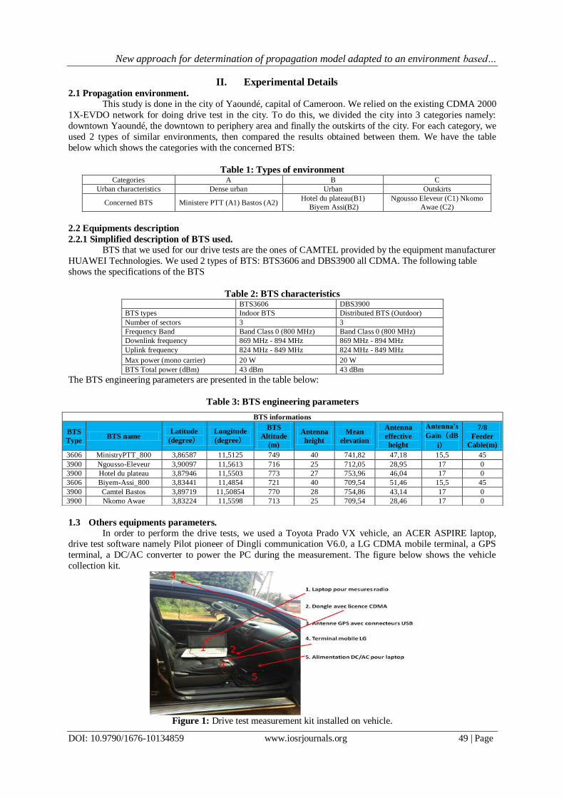
1.3 Others equipments parameters.

In order to perform the drive tests, we used a Toyota Prado VX vehicle, an ACER ASPIRE laptop, drive test software namely Pilot pioneer of Dingli communication V6.0, a LG CDMA mobile terminal, a GPS

terminal, a DC/AC converter to power the PC during the measurement. The figure below shows the vehicle

collection kit.

Figure 1: Drive test measurement kit installed on vehicle.

BTS informations

BTS

Type BTS name

Latitude

(degree）

Longitude

(degree）

BTS

Altitude

(m)

Antenna

height

Mean

elevation

Antenna

effective

height

Antenna’s

Gain（dB

i）

7/8

Feeder

Cable(m)

3606 MinistryPTT_800 3,86587 11,5125 749 40 741,82 47,18 15,5 45

3900 Ngousso-Eleveur 3,90097 11,5613 716 25 712,05 28,95 17 0

3900 Hotel du plateau 3,87946 11,5503 773 27 753,96 46,04 17 0

3606 Biyem-Assi_800 3,83441 11,4854 721 40 709,54 51,46 15,5 45

3900 Camtel Bastos 3,89719 11,50854 770 28 754,86 43,14 17 0

3900 Nkomo Awae 3,83224 11,5598 713 25 709,54 28,46 17 0

New approach for determination of propagation model adapted to an environment based…

DOI: 10.9790/1676-10134859 www.iosrjournals.org 50 | Page

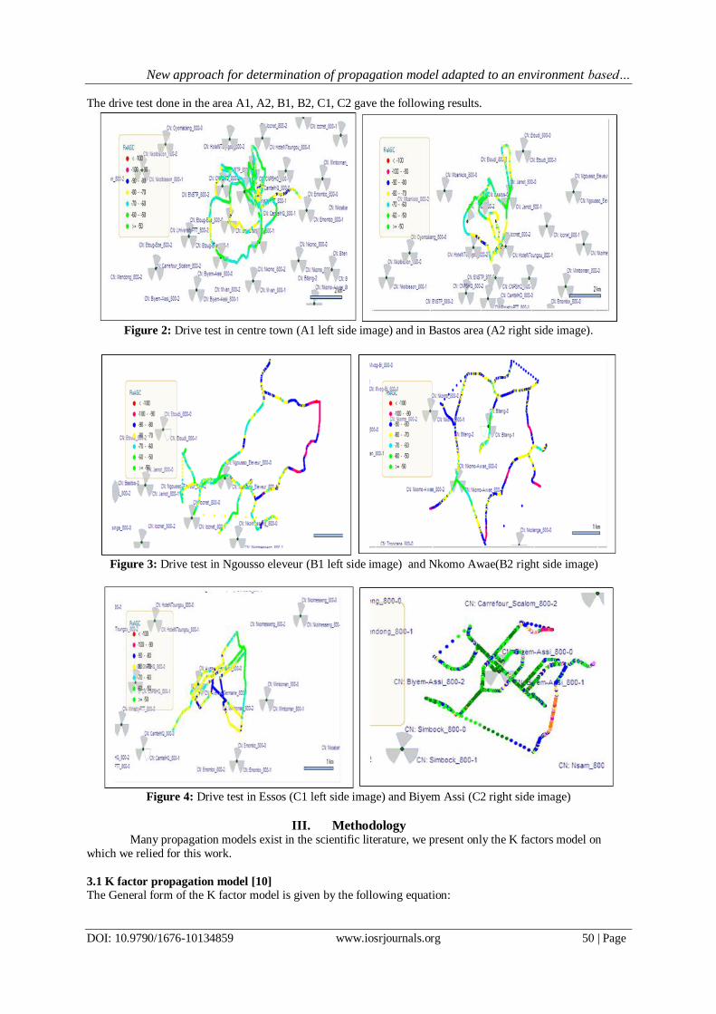
The drive test done in the area A1, A2, B1, B2, C1, C2 gave the following results.

Figure 2: Drive test in centre town (A1 left side image) and in Bastos area (A2 right side image).

Figure 3: Drive test in Ngousso eleveur (B1 left side image) and Nkomo Awae(B2 right side image)

Figure 4: Drive test in Essos (C1 left side image) and Biyem Assi (C2 right side image)

III. Methodology Many propagation models exist in the scientific literature, we present only the K factors model on

which we relied for this work.

3.1 K factor propagation model [10]

The General form of the K factor model is given by the following equation:

New approach for determination of propagation model adapted to an environment based…

DOI: 10.9790/1676-10134859 www.iosrjournals.org 51 | Page

𝑳𝒑 =

𝑲𝟏 + 𝑲𝟐 𝒍𝒐𝒈 𝒅 + 𝑲𝟑 ∗ 𝒉𝒎 + 𝑲𝟒 ∗ 𝒍𝒐𝒈 𝒉𝒎 + 𝑲𝟓 ∗ 𝒍𝒐𝒈 𝒉𝒃 + 𝑲𝟔 ∗ 𝒍𝒐𝒈 𝒉𝒃 𝒍𝒐𝒈 𝒅 + 𝑲𝟕𝒅𝒊𝒇𝒇𝒏+ 𝑲𝒄𝒍𝒖𝒕𝒕𝒆𝒓

(1)

𝑲𝟏 Constant related to the frequency, 𝑲𝟐 Constant of attenuation of the distance or propagation exponent, 𝑲𝟑

and 𝑲𝟒 are correction factors of mobile station height; 𝑲𝟓 and 𝑲𝟔 are correction factors of BTS height, 𝑲𝟕 is

the diffraction factor, and 𝑲𝒄𝒍𝒖𝒕𝒕𝒆𝒓 correction factor due to clutter type.

The K parameter values vary depending on the type of terrain and the characteristics of the propagation of the

city environment; the following table gives values of K for a medium-sized town.

Table 4: K factor parameters values

The above equation (1) could also be written in the following form:

𝑳𝒑 =

(𝑲𝟏 + 𝑲𝟕𝒅𝒊𝒇𝒇𝒏+ 𝑲𝒄𝒍𝒖𝒕𝒕𝒆𝒓) + 𝑲𝟐 𝒍𝒐𝒈 𝒅 + 𝑲𝟑 ∗ 𝒉𝒎 + 𝑲𝟒 ∗ 𝒍𝒐𝒈 𝒉𝒎 + 𝑲𝟓 ∗ 𝒍𝒐𝒈(𝒉𝒃) + 𝑲𝟔 𝒍𝒐𝒈 𝒉𝒃 𝒍𝒐𝒈(𝒅)

Assuming 𝐾1′ = (𝐾1 + 𝐾7𝑑𝑖𝑓𝑓𝑛 + 𝐾𝑐𝑙𝑢𝑡𝑡𝑒𝑟 ) , equation (1) gets the form below:

𝑳𝒑 = 𝑲𝟏 + 𝑲𝟐 𝒍𝒐𝒈 𝒅 + 𝑲𝟑 ∗ 𝒉𝒎 + 𝑲𝟒 ∗ 𝒍𝒐𝒈 𝒉𝒎 + 𝑲𝟓 ∗ 𝒍𝒐𝒈(𝒉𝒃) + 𝑲𝟔 𝒍𝒐𝒈 𝒉𝒃 𝒍𝒐𝒈(𝒅) (2)

It is this last modified form that we will eventually use for our work.

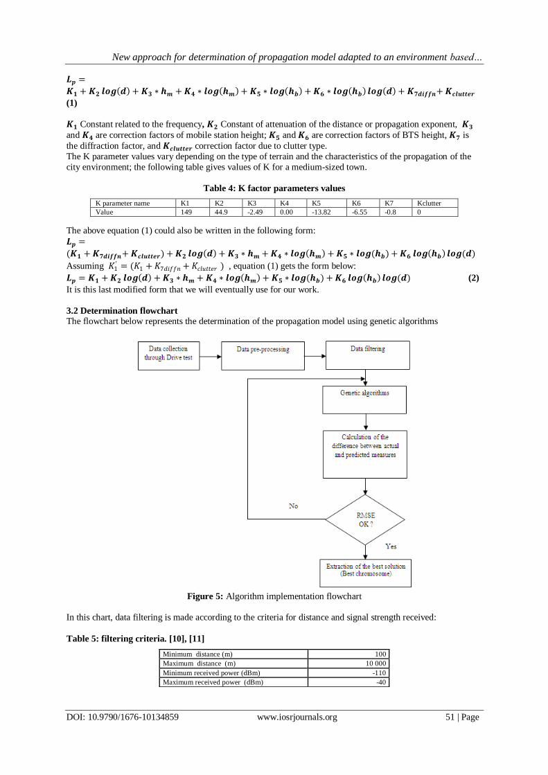
3.2 Determination flowchart

The flowchart below represents the determination of the propagation model using genetic algorithms

Figure 5: Algorithm implementation flowchart

In this chart, data filtering is made according to the criteria for distance and signal strength received:

Table 5: filtering criteria. [10], [11]

K parameter name K1 K2 K3 K4 K5 K6 K7 Kclutter

Value 149 44.9 -2.49 0.00 -13.82 -6.55 -0.8 0

Minimum distance (m) 100

Maximum distance (m) 10 000

Minimum received power (dBm) -110

Maximum received power (dBm) -40

New approach for determination of propagation model adapted to an environment based…

DOI: 10.9790/1676-10134859 www.iosrjournals.org 52 | Page

3.3 Genetic algorithms. [12]

A genetic algorithm enables us to find a solution by searching an extremum (maximum or minimum)

on a set of possible solutions, the solution set is called search space. This algorithm is built following the points below:

• The coding of the elements of the population (chromosomes),

• The generation of the initial population,

• Evaluation of each chromosome of the population

• Selection, crossover and mutation of chromosomes,

• Criteria to stop the algorithm.

3.3.1 Modeling of our problem by genetic algorithms.

It is a question for us to find a propagation model to suit any environment.

Equation (2) above can be written in matrix form as follows:

𝑳 = [𝑲𝟏 𝑲𝟐 𝑲𝟑𝑲𝟒 𝑲𝟓 𝑲𝟔 ] ∗

𝟏𝒍𝒐𝒈(𝒅)𝑯𝒎

𝒍𝒐𝒈(𝑯𝒎)𝒍𝒐𝒈(𝑯𝒆𝒇𝒇)

𝒍𝒐𝒈(𝑯𝒆𝒇𝒇) ∗ 𝒍𝒐𝒈(𝒅)

(3)

In the above equation (3) only the vector K= 𝐾1 𝐾2 𝐾3𝐾4 𝐾5 𝐾6 (4) is variable depending on the values

of, 𝑖 𝟄 𝟏, 𝟐,𝟑, 𝟒,𝟓,𝟔 and j an integer.

Let:

𝑴 =

𝟏𝒍𝒐𝒈(𝒅)𝑯𝒎

𝒍𝒐𝒈(𝑯𝒎)𝒍𝒐𝒈(𝑯𝒆𝒇𝒇)

𝒍𝒐𝒈(𝑯𝒆𝒇𝒇) ∗ 𝒍𝒐𝒈(𝒅)

, (5)

Therefore L can be written in the form 𝐿 = 𝐾 ∗ 𝑀 (6); with M a constant vector for a given distance d and

depending on whether we were under a base station of effective height 𝐻𝑒𝑓𝑓 .

If in the contrary the distance d varies for different measurement points, vector M becomes a 𝑀𝑖vector for

various measures at different distances 𝑑𝑖 points.

The determination of the vector K leads to the knowledge of our propagation model L. Our searching area is therefore that containing all the possible values of the vectors of the form presented as K above in (4).

So we will use a real coding as chromosomes K vectors as presented above.

It is therefore necessary for us to model the elements forming part of our genetic algorithm namely: the genes

encoding type, the generation of the initial family, the evaluation function of each chromosome, the selection

method, crossover and the mutation algorithms.

3.3.1.1 Genetic algorithm parameters

Subsequently we will consider the following parameters:

• Ng, the number of generations,

• Nc, the number of chromosomes of the family at any generation,

• Tc and Tm respectively crossing and mutation rates.

3.3.1.2 Encoding type.

We will use a real coding [13] representing our chromosomes in the vector form given by equation (4)

above. Our chromosomes will be the K vectors.

3.3.1.3 Evaluation function. Here, we have to minimize the Euclidean distance between the measured values of the propagation loss

and those predicted by the propagation model. Let 𝐿 = 𝐿𝑗 𝑗=1:𝑇 the set of measured values; where T represents

the total number of measurement points of L. 𝐾𝑗 is a possible solution vector to our optimization problem and

𝑀𝑖 the column vector defined by (5). The evaluation function [14] of our chromosomes 𝐾𝑗 will be:

𝒇𝒄𝒐𝒖𝒕 = 𝒎𝒊𝒏 𝟏

𝑻 (𝑳𝒊 − 𝑲𝒋 ∗𝑴𝒊 )𝟐𝑻

𝒊=𝟏 . (6)

This is for every chromosome 𝐾𝑗 for j=1: Nc.

New approach for determination of propagation model adapted to an environment based…

DOI: 10.9790/1676-10134859 www.iosrjournals.org 53 | Page

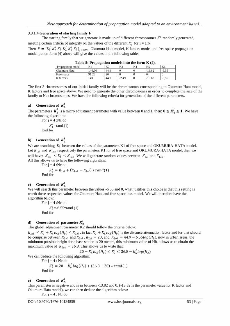
3.3.1.4 Generation of starting family F

The starting family that we generate is made up of different chromosomes 𝐾𝑗 randomly generated,

meeting certain criteria of integrity on the values of the different 𝐾𝑖𝑗 for i = 1:6.

Then 𝐹 = [𝐾1𝑗 𝐾2

𝑗 𝐾3

𝑗 𝐾4

𝑗 𝐾5

𝑗 𝐾6

𝑗]𝑗=1:𝑁𝑐 . Okumura Hata model, K factors model and free space propagation

model put on form (4) above will give the values in the following table:

Table 5: Propagation models into the form K (4). Propagation model K1 K2 K3 K4 K5 K6

Okumura Hata 146,56 44.9 0 0 -13.82 -6,55

Free space 91.28 20 0 0 0 0

K factors 149 44.9 -2.49 0 -13.82 -6,55

The first 3 chromosomes of our initial family will be the chromosomes corresponding to Okumura Hata model,

K factors and free space above. We need to generate the other chromosomes in order to complete the size of the

family to Nc chromosomes. We have the following criteria for generation of the different parameters.

a) Generation of 𝑲𝟒𝒋

The parameters 𝑲𝟒𝒋 is a micro adjustment parameter with value between 0 and 1, then: 𝟎 ≤ 𝑲𝟒

𝒋≤ 𝟏. We have

the following algorithm:

For j = 4 :Nc do

𝐾4𝑗=rand (1)

End for

b) Generation of 𝑲𝟏𝒋

We are searching 𝐾1𝑗 between the values of the parameters K1 of free space and OKUMURA-HATA model.

Let 𝐾1𝑒𝑙 and 𝐾1𝑜𝑘 respectively the parameters K1 for of free space and OKUMURA-HATA model, then we

will have: 𝐾1𝑒𝑙 ≤ 𝐾1𝑗≤ 𝐾1𝑜𝑘 . We will generate random values between 𝐾1𝑒𝑙 and 𝐾1𝑜𝑘 .

All this allows us to have the following algorithm:

For j = 4 :Nc do

𝐾1𝑗

= 𝐾1𝑒𝑙 + 𝐾1𝑜𝑘 −𝐾1𝑒𝑙 ∗ 𝑟𝑎𝑛𝑑(1)

End for

c) Generation of 𝑲𝟔𝒋

We will search this parameter between the values -6.55 and 0, what justifies this choice is that this setting is

worth these respective values for Okumura Hata and free space loss model. We will therefore have the

algorithm below:

For j = 4 :Nc do

𝐾6𝑗=-6.55*rand (1)

End for

d) Generation of parameter 𝑲𝟐𝒋

The global adjustment parameter K2 should follow the criteria below:

𝐾2𝑒𝑙 ≤ 𝐾2𝑗

+ 𝐾6𝑗𝑙𝑜𝑔(𝐻𝑏) ≤ 𝐾2𝑜𝑘 , in fact 𝐾2

𝑗+ 𝐾6

𝑗𝑙𝑜𝑔(𝐻𝑏) is the distance attenuation factor and for that should

be comprise between 𝐾2𝑒𝑙 and 𝐾2𝑜𝑘 . 𝐾2𝑒𝑙 = 20, and 𝐾2𝑜𝑘 = 44.9 − 6.55𝑙𝑜𝑔(𝐻𝑏), now in urban areas, the

minimum possible height for a base station is 20 meters, this minimum value of Hb, allows us to obtain the

maximum value of 𝐾2𝑜𝑘 = 36.8. This allows us to write that:

20 −𝐾6𝑗𝑙𝑜𝑔(𝐻𝑏) ≤ 𝐾2

𝑗≤ 36.8 − 𝐾6

𝑗𝑙𝑜𝑔(𝐻𝑏)

We can deduce the following algorithm: For j = 4 : Nc do

𝐾2𝑗

= 20 − 𝐾6𝑗𝑙𝑜𝑔 𝐻𝑏 + 36.8 − 20 ∗ 𝑟𝑎𝑛𝑑(1)

End for

e) Generation of 𝑲𝟓𝒋

This parameter is negative and is in between -13.82 and 0. (-13.82 is the parameter value for K factor and

Okumura Hata model), we can then deduce the algorithm below:

For j = 4 : Nc do

New approach for determination of propagation model adapted to an environment based…

DOI: 10.9790/1676-10134859 www.iosrjournals.org 54 | Page

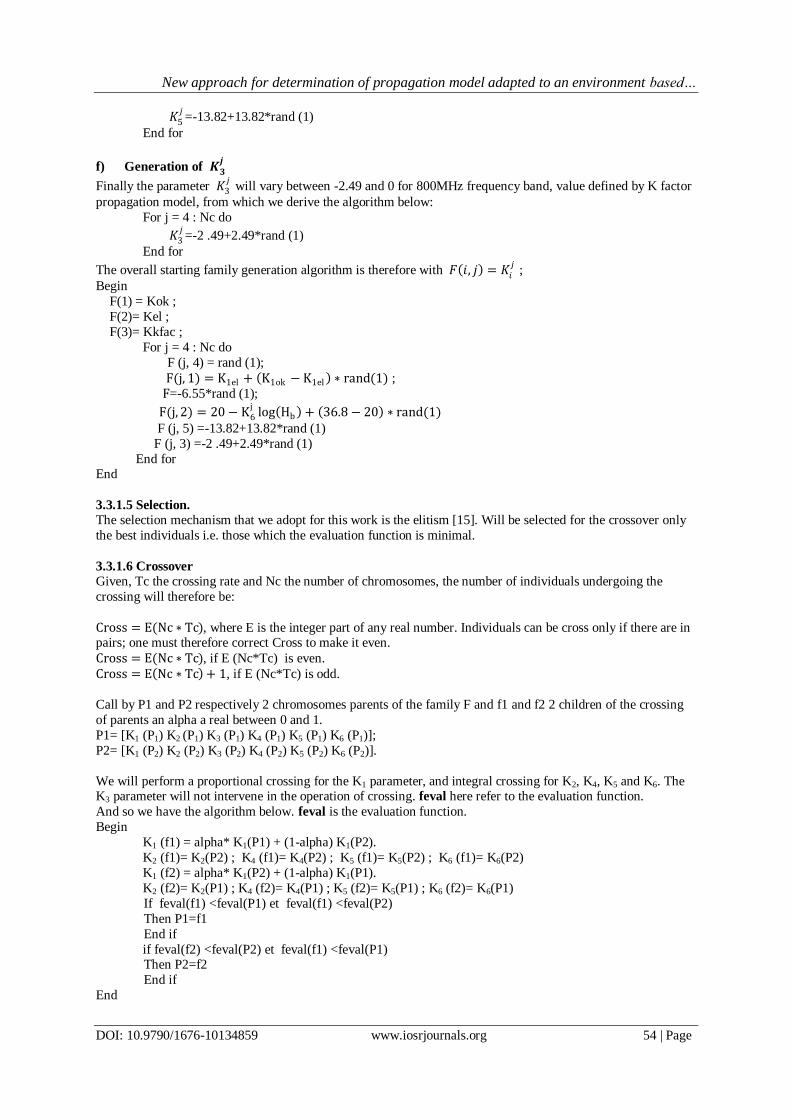
𝐾5𝑗=-13.82+13.82*rand (1)

End for

f) Generation of 𝑲𝟑𝒋

Finally the parameter 𝐾3𝑗 will vary between -2.49 and 0 for 800MHz frequency band, value defined by K factor

propagation model, from which we derive the algorithm below:

For j = 4 : Nc do

𝐾3𝑗=-2 .49+2.49*rand (1)

End for

The overall starting family generation algorithm is therefore with 𝐹 𝑖, 𝑗 = 𝐾𝑖𝑗 ;

Begin

F(1) = Kok ;

F(2)= Kel ;

F(3)= Kkfac ;

For j = 4 : Nc do

F (j, 4) = rand (1);

F(j, 1) = K1el + K1ok − K1el ∗ rand(1) ;

F=-6.55*rand (1);

F(j, 2) = 20 − K6j

log Hb + 36.8 − 20 ∗ rand(1)

F (j, 5) =-13.82+13.82*rand (1)

F (j, 3) =-2 .49+2.49*rand (1)

End for End

3.3.1.5 Selection.

The selection mechanism that we adopt for this work is the elitism [15]. Will be selected for the crossover only

the best individuals i.e. those which the evaluation function is minimal.

3.3.1.6 Crossover

Given, Tc the crossing rate and Nc the number of chromosomes, the number of individuals undergoing the

crossing will therefore be:

Cross = E(Nc ∗ Tc), where E is the integer part of any real number. Individuals can be cross only if there are in pairs; one must therefore correct Cross to make it even.

Cross = E(Nc ∗ Tc), if E (Nc*Tc) is even.

Cross = E Nc ∗ Tc + 1, if E (Nc*Tc) is odd.

Call by P1 and P2 respectively 2 chromosomes parents of the family F and f1 and f2 2 children of the crossing

of parents an alpha a real between 0 and 1.

P1= [K1 (P1) K2 (P1) K3 (P1) K4 (P1) K5 (P1) K6 (P1)];

P2= [K1 (P2) K2 (P2) K3 (P2) K4 (P2) K5 (P2) K6 (P2)].

We will perform a proportional crossing for the K1 parameter, and integral crossing for K2, K4, K5 and K6. The K3 parameter will not intervene in the operation of crossing. feval here refer to the evaluation function.

And so we have the algorithm below. feval is the evaluation function.

Begin

K1 (f1) = alpha* K1(P1) + (1-alpha) K1(P2).

K2 (f1)= K2(P2) ; K4 (f1)= K4(P2) ; K5 (f1)= K5(P2) ; K6 (f1)= K6(P2)

K1 (f2) = alpha* K1(P2) + (1-alpha) K1(P1).

K2 (f2)= K2(P1) ; K4 (f2)= K4(P1) ; K5 (f2)= K5(P1) ; K6 (f2)= K6(P1)

If feval(f1) <feval(P1) et feval(f1) <feval(P2)

Then P1=f1

End if

if feval(f2) <feval(P2) et feval(f1) <feval(P1) Then P2=f2

End if

End

New approach for determination of propagation model adapted to an environment based…

DOI: 10.9790/1676-10134859 www.iosrjournals.org 55 | Page

6.1.1.1 Mutation

Here considering that the rate of mutation is Tm, we will mutate individuals that have not been involved

in crossover mechanism to give them a chance to improve so if possible to participate in the next reproduction. We will therefore choose random individuals then mutate them and replace the old (parent or former) by the

mutants. The mutation will operate on a global adjustment parameter, the number of possible mutations is:

Nmut = E(Tm * Nc * 6) + 1 (6 is the size of a Chromosome).

The algorithm of mutation is given below:

Begin

Nmut = E (tm * Nc * 6) +1

For i=1: Nmut

mut= E (cross+1+(Nc-(cross+1)) * rand(1)) + 1

F(mut,2)=20 - F(mut,6)*log(Hb) +16.38*rand(1);

End

IV. Results And Comments Having implemented the genetic algorithm as described above on the radio measurement data obtained

in Yaoundé by setting the parameters as follows:

Nc = 60; NG = 100; Tc = 0.6; Tm = 0.01; alpha = 0.6, we obtained the results as presented below. NG is the

number of generations, Nc the number of chromosomes.

The model will be seen as accurate if the RMSE between the values of prediction and measured is less than 8

dB; (RMSE < 8dB). [16]

4.1 Results per zone We obtained the representatives curves below, the actual measurements are in blue, Okumura Hata

model in green, and the free space propagation model in yellow, the new model obtained via Genetic

Algorithms in red and that obtained by implementing the linear regression in black. In the following tables,

RMSE (OK) will refer to the RMSE calculate using Okumura Hata model relatively to drive test datas.

a) Zone A1 : Yaoundé centre town.

Figure 6: Actual data in Centre town VS predicted measurements.

The table below gives the results of genetic algorithms and linear regression.

Table 6: Results from the city center. Zone Methode K1 K2 K3 K4 K5 K6 RMSE RMSE(OK)

A1

GA 125.6569 34.4485 -2.4900 0 -4.6067 -6.55 6.5704

14.9345

Lin

Regression 134.8893 37.2911 -2.4900 0 -13.8200 -6.55 6.7137

New approach for determination of propagation model adapted to an environment based…

DOI: 10.9790/1676-10134859 www.iosrjournals.org 56 | Page

Note that we have a RMSE <8dB which confirms the reliability of the result and better than RMSE(OK).

b) Zone A2 : Bastos area (Ambassy quaters)

Figure 7: Actual data in Bastos VS predicted measurements.

The table below gives the results of genetic algorithms and linear regression.

Table 7: Results from bastos area. Zone Methode K1 K2 K3 K4 K5 K6 RMSE RMSE(OK)

A2 GA 125.6569 34.4485 -2.4900 0 -4.6067 -6.55 6.5704

11,2924 Lin regression 138.9332 27.7118 -2.4900 0 -13.8200 -6.55 6.1059

Note that we have a RMSE <8dB which confirms the reliability of the result and better than RMSE(OK).

c) Zone B1 : Biyem Assi area

Figure 8: Actual data in Biyem Assi VS predicted measurements.

The table below gives the results of genetic algorithms and linear regression.

Table 8: Results from Biyem Assi area. Zone Methode K1 K2 K3 K4 K5 K6 RMSE RMSE(OK)

B1 GA 121.3351 35.1371 -2.4900 0 -4.8370 -6.55 6.1845

12,3604 Lin Regression 131.9004 23.1678 -2.4900 0 -13.820 -6.55 5.3883

Note that we have a RMSE <8dB which confirms the reliability of the result and better than RMSE(OK).

a) Zone B2 : Essos-Mvog Ada area

The table below gives the results of genetic algorithms and linear regression.

New approach for determination of propagation model adapted to an environment based…

DOI: 10.9790/1676-10134859 www.iosrjournals.org 57 | Page

Table 9: Results from Essos Mvog Ada area. Zone Methode K1 K2 K3 K4 K5 K6 RMSE RMSE(OK)

B2 GA 127.8881 35.3815 -2.4900 0 -5.5280 -6.55 7.3976

11,5989 Lin Regression 141.7505 36.5336 -2.4900 0 -13.82 -6.55 7.3907

Note that we have a RMSE <8dB which confirms the reliability of the result and better than RMSE(OK).

Figure 9: Actual data in Essos Camp Sonel area VS predicted measurements.

e) Zone C1 : Quartier Ngousso Eleveur

Figure 10: Actual data in Ngousso Eleveur area VS predicted measurements.

The table below gives the results of genetic algorithms and linear regression.

Table 10: Results from Ngousso Eleveur area. Zone Methode K1 K2 K3 K4 K5 K6 RMSE RMSE(OK)

C1 GA 122.4182 32.5658 -2.4900 0 -3.6853 -6.55 7.8990

16,8067 Lin Regression 137.3067 31.8195 -2.4900 0 -13.82 -6.55 7.8927

Note that we have a RMSE <8dB which confirms the reliability of the result and better than RMSE (OK).

Zone C2: Nkomo Awae area

New approach for determination of propagation model adapted to an environment based…

DOI: 10.9790/1676-10134859 www.iosrjournals.org 58 | Page

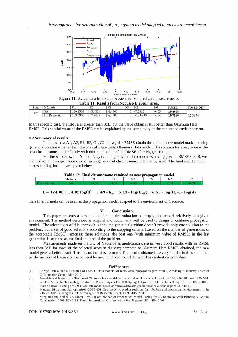
Figure 11: Actual data in nkomo Awae area VS predicted measurements.

Table 11: Results from Ngousso Eleveur area. Zone Méthode K1 K2 K3 K4 K5 K6 RMSE RMSE(OK)

C2 GA 130.9568 45.4324 -2.4900 0 -7.8313 -6.55 10.8068

15,3274 Lin Regression 139.4966 47.7877 -2.4900 0 -13.8200 -6.55 10.7990

In this specific case, the RMSE is greater than 8dB, but the value obtain is still better than Okumura Hata RMSE. This special value of the RMSE can be explained by the complexity of the concerned environnement.

4.2 Summary of results

In all the area A1, A2, B1, B2, C1, C2 above, the RMSE obtain through the new model made up using

genetic algorithm is better than the one calculate using Okumura Hata model. The solution for every zone is the

best chromosomes in the family with minimum value of the RMSE after Ng generations.

For the whole town of Yaoundé, by retaining only the chromosomes having given a RMSE < 8dB, we

can deduce an average chromosome (average value of chromosomes retained by area). The final result and the

corresponding formula are given below.

Table 12: Final chromosome retained as new propagation model

Methode K1 K2 K3 K4 K5 K6

Final solution GA 124,08 34,82 -2,49 0 -5,11 -6,55

𝐋 = 𝟏𝟐𝟒.𝟎𝟖 + 𝟑𝟒. 𝟖𝟐𝐥𝐨𝐠 𝐝 − 𝟐. 𝟒𝟗 ∗ 𝐡𝐦 − 𝟓.𝟏𝟏 ∗ 𝐥𝐨𝐠 𝐇𝐞𝐟𝐟 − 𝟔.𝟓𝟓 ∗ 𝐥𝐨𝐠 𝐇𝐞𝐟𝐟 ∗ 𝐥𝐨𝐠(𝐝)

This final formula can be seen as the propagation model adapted to the environment of Yaoundé.

V. Conclusion. This paper presents a new method for the determination of propagation model relatively to a given

environment. The method described is original and could very well be used to design or calibrate propagation

models. The advantages of this approach is that, the genetic algorithm doesn’t provide only one solution to the

problem, but a set of good solutions according to the stopping criteria (based on the number of generations or

the acceptable RMSE), amongst these solutions, the best one (with minimum value of RMSE) in the last

generation is selected as the final solution of the problem.

Measurements made on the city of Yaoundé as application gave us very good results with an RMSE

less than 8dB for most of the selected areas in the city; compare to Okumura Hata RMSE obtained, the new

model gives a better result .This means that it is accurate. The results obtained are very similar to those obtained

by the method of linear regression used by most authors around the world as calibration procedure.

Références [1]. Chhaya Dalela, and all « tuning of Cost231 Hata modele for radio wave propagation prediction », Academy & Industry Research

Collaboration Center, May 2012.

[2]. Medeisis and Kajackas « The tuned Okumura Hata model in urban and rural zones at Lituania at 160, 450, 900 and 1800 MHz

bands », Vehicular Technology Conference Proceedings, VTC 2000-Spring Tokyo. IEEE 51st Volume 3 Pages 1815 – 1818, 2000.

[3]. Prasad and al « Tuning of COST-231Hata model based on various data sets generated over various regions of India »,

[4]. Mardeni &Priya and All, optimized COST-231 Hata model to predict path loss for suburban and open urban environments in the

2360-2390MHz, Progress In Electromagnetics Research C, Vol. 13, 91-106, 2010.

[5]. MingjingYang; and al « A Linear Least Square Method of Propagation Model Tuning for 3G Radio Network Planning », Natural

Computation, 2008. ICNC '08. Fourth International Conference on Vol. 5, pages 150 – 154, 2008.

New approach for determination of propagation model adapted to an environment based…

DOI: 10.9790/1676-10134859 www.iosrjournals.org 59 | Page

[6]. Chen, Y.H. and Hsieh, K.L « A Dual Least-Square Approach of Tuning Optimal Propagation Model for existing 3G Radio

Network », Vehicular Technology Conference, 2006. VTC 2006-Spring. IEEE 63rd Vol. 6, pages 2942 – 2946, 2006.

[7]. Simi I.S and al « Minimax LS algorithm for automatic propagation model tuning », Proceeding of the 9th Telecommunications

Forum (TELFOR 2001), Belgrade, Nov.2001.

[8]. Allam Mousa, Yousef Dama and Al «Optimizing Outdoor Propagation Model based on Measurements for Multiple RF Cell ».

International Journal of Computer Applications (0975 – 8887) Volume 60– No.5, December 2012

[9]. HUAWEI Technologies, BTS3606CE&BTS3606AC and 3900 Series CDMA Product Documentation, pages 138-139.

[10]. HUAWEI Technologies, CW Test and Propagation Model Tuning Report (Template), 20 Mars 2014, page 7.

[11]. Standard Propagation Model Calibration guide, Avril 2004, page 23.

[12]. Ricardo Salem Zebulum, Marco Aurélio and al, Evolutionary Electronics: Automatic Design of Electronic Circuits and Systems by

Genetic AlgorithmsEvolutionnary, pages 25-27, 2002.

[13]. D.E Goldberg. Real-coded genetic algorithms, virtual alphabets and blocking. Complex Systems, 1991. Pages 139-167,

[14]. Allam Mousa and all, Optimizing Outdoor Propagation Model based on Measurements for Multiple RF Cell, International Journal

of Computer Applications (0975 – 8887) Volume 60– No.5, December 2012.

[15]. Ricardo Salem Zebulum, Marco Aurélio and al, Evolutionary Electronics: Automatic Design of Electronic Circuits and Systems by

Genetic Algorithms Evolutionnary, 2002, pages 32-35.

[16]. A. Bhuvaneshwari, R. Hemalatha, T. Satyasavithri ;Statistical Tuning of the Best suited Prediction Model for Measurements made

in Hyderabad City of Southern India. Proceedings of the World Congress on Engineering and Computer Science 2013 Vol II

WCECS 2013, San Francisco, USA pages 23-25 October, 2013.

View publication statsView publication stats