Embed Size (px)
Citation preview
New approaches to protein docking
Dissertation zur Erlangung des GradesDoktor der Ingenieurwissenschaften (Dr.-Ing.)
der Naturwissenschaftlich-Technischen Fakultat Ider Universitat des Saarlandes
von
Oliver Kohlbacher
Saarbrucken12. Januar 2001

Datum des Kolloquiums: 12. Januar 2000
Dekan der technischen Fakultat:Professor Dr. Rainer Schulze-Pillot-Ziemen
Gutachter:Professor Dr. Hans-Peter Lenhof, Universitat des Saarlandes, SaarbruckenProfessor Dr. Kurt Mehlhorn, MPI fur Informatik, Saarbrucken
2

\I think the most ex iting omputer resear h now is partly in roboti s, and partlyin appli ations to bio hemistry.. . .Biology is so digital, and in redibly ompli ated, but in redibly useful. The troublewith biology is that, if you have to work as a biologist, it's boring. Your experimentstake you three years and then, one night, the ele tri ity goes o� and all the thingsdie! You start over. In omputers we an reate our own worlds. Biologists deservea lot of redit for being able to slug it through." – Donald Knuth
Acknowledgements
The work on this thesis was carried out during the years 1996–2000 at the Max-Planck-Institut fur Informatik in the group of Prof. Dr. Kurt Mehlhorn under the supervision ofProf. Dr. Hans-Peter Lenhof.
Prof. Dr. Hans-Peter Lenhof kindled my interest in Bioinformatics and gave me the freedomto do research in those areas that fascinated me most. Our discussions, although sometimesheated, were always fruitful and forced me to get to the very bottom of many problems.
The implementation of BALL is unthinkable without the help of all the people who con-tributed code and ideas. Nicolas Boghossian had significantimpact on the design of the librarycore and contributed lots of code for the kernel. Heiko Kleinimplemented the largest part ofthe visualization. Dr. Peter Muller brought in his experience in the field of molecular dynamicssimulations. Andreas Burchardt implemented parts of the NMR code. Upon Andreas Moll fellthe ungrateful work of testing and debugging. Stefan Strobel implemented the difficult partof molecular surface calculations. Andreas Hildebrandt implemented the NMR visualization.The more sophisticated parts of the solvation code were implemented by Andreas Kerzmann,who also set up the BALL web server. Last, but not least, Prof.Dr. Hans-Peter Lenhof not onlycontributed code for structure mapping and force field calculations, but also initiated the wholeproject and kept everyone motivated.
Ernst Althaus implemented the branch-&-cut-algorithm andwas coauthor of the paper onflexible docking. He had the patience to explain to me some of the finer details of polyhedraltheory.
The Rechnerbetriebsgruppe had to suffer from this work as well. Jorg Herrmann, WolframWagner, Bernd Farber, Uwe Brahm, Thomas Hirtz, and Roland Berberich solved numerous ofmy hardware- and software-related problems even at night and during weekends. ChristophClodo managed to track down and resolve several errors in theLATEX code of this thesis.
I am also grateful to my “WG” (Holger, Michael, Christian) for nearly six years of enjoy-able coexistence and for the flat, the evenings, and quite some bottles of wine we shared. Last,but certainly not least, I wish to thank Andreas for his patience, his understanding, and hissupport while I wrote this thesis.

Abstract
In the first part of this work, we propose new methods for protein docking. First, we present two ap-proaches to protein docking with flexible side chains. The first approach is a fast greedy heuristic, whilethe second is a branch-&-cut algorithm that yields optimal solutions. For a test set of protease-inhibitorcomplexes, both approaches correctly predict the true complex structure. Another problem in proteindocking is the prediction of the binding free energy, which is the the final step of many protein dockingalgorithms. Therefore, we propose a new approach that avoids the expensive and difficult calculation ofthe binding free energy and, instead, employs a scoring function that is based on the similarity of theproton nuclear magnetic resonance spectra of the tentativecomplexes with the experimental spectrum.Using this method, we could even predict the structure of a very difficult protein-peptide complex thatcould not be solved using any energy-based scoring functions.
The second part of this work presents BALL (Biochemical ALgorithms Library), a framework forRapid Application Development in the field of Molecular Modeling. BALL provides an extensive setof data structures as well as classes for Molecular Mechanics, advanced solvation methods, comparisonand analysis of protein structures, file import/export, NMRshift prediction, and visualization. BALLhas been carefully designed to be robust, easy to use, and open to extensions. Especially its extensibility,which results from an object-oriented and generic programming approach, distinguishes it from othersoftware packages.
Kurzzusammenfassung
Der erste Teil dieser Arbeit beschaftigt sich mit neuen Ansatzen zum Proteindocking. Zunachst stellenwir zwei Ansatze zum Proteindocking mit flexiblen Seitenketten vor. Der erste Ansatz beruht auf einerschnellen, gierigen Heuristik, wahrend der zweite Ansatzauf branch-&-cut-Techniken beruht und dasProblem optimal losen kann. Beide Ansatze sind in der Lagedie korrekte Komplexstruktur fur einenSatz von Testbeispielen (bestehend aus Protease-Inhibitor-Komplexen) vorherzusagen. Ein weiteres,grosstenteils ungelostes, Problem ist der letzte Schritt vieler Protein-Docking-Algorithmen, die Vorher-sage der freien Bindungsenthalpie. Daher schlagen wir eineneue Methode vor, die die schwierige undaufwandige Berechnung der freien Bindungsenthalpie vermeidet. Statt dessen wird eine Bewertungs-funktion eingesetzt, die auf derAhnlichkeit der Protonen-Kernresonanzspektren der potentiellen Kom-plexstrukturen mit dem experimentellen Spektrum beruht. Mit dieser Methode konnten wir sogar diekorrekte Struktur eines Protein-Peptid-Komplexes vorhersagen, an dessen Vorhersage energiebasierteBewertungsfunktionen scheitern.
Der zweite Teil der Arbeit stellt BALL (Biochemical ALgorithms Library) vor, ein Rahmenwerkzur schnellen Anwendungsentwicklung im Bereich MolecularModeling. BALL stellt eine Vielzahl vonDatenstrukturen und Algorithmen fur die Felder Molekulmechanik, Vergleich und Analyse von Protein-strukturen, Datei-Import und -Export, NMR-Shiftvorhersage und Visualisierung zur Verfugung. BeimEntwurf von BALL wurde auf Robustheit, einfache Benutzbarkeit und Erweiterbarkeit Wert gelegt.Von existierenden Software-Paketen hebt es sich vor allem durch seine Erweiterbarkeit ab, die auf derkonsequenten Anwendung von objektorientierter und generischer Programmierung beruht.


Contents
Part I – Introduction 1
Part II – Protein Docking 7
1 Biochemistry – the Basics 91.1 Atoms and Molecules . . . . . . . . . . . . . . . . . . . . . . . . . . . . . . .91.2 Amino Acids . . . . . . . . . . . . . . . . . . . . . . . . . . . . . . . . . . . 101.3 Proteins . . . . . . . . . . . . . . . . . . . . . . . . . . . . . . . . . . . . . . 101.4 Nucleic Acids . . . . . . . . . . . . . . . . . . . . . . . . . . . . . . . . . . . 131.5 Interatomic Forces . . . . . . . . . . . . . . . . . . . . . . . . . . . . . . .. 14
1.5.1 Nonbonded interactions . . . . . . . . . . . . . . . . . . . . . . . . .141.5.2 Molecular Mechanics . . . . . . . . . . . . . . . . . . . . . . . . . . . 16
2 Introduction 192.1 Rigid Body Docking . . . . . . . . . . . . . . . . . . . . . . . . . . . . . . . 192.2 Docking and Protein Flexibility . . . . . . . . . . . . . . . . . . . .. . . . . . 212.3 Combining NMR Data and Docking Algorithms . . . . . . . . . . . .. . . . . 23
3 Semi-Flexible Docking 253.1 Introduction . . . . . . . . . . . . . . . . . . . . . . . . . . . . . . . . . . . .253.2 The Docking Algorithm . . . . . . . . . . . . . . . . . . . . . . . . . . . . .. 28
3.2.1 Rigid Docking . . . . . . . . . . . . . . . . . . . . . . . . . . . . . . 283.2.2 Side Chain Demangling . . . . . . . . . . . . . . . . . . . . . . . . . 283.2.3 The Multi-Greedy Method . . . . . . . . . . . . . . . . . . . . . . . . 293.2.4 The Branch-&-Cut Algorithm . . . . . . . . . . . . . . . . . . . . . .303.2.5 Energetic Evaluation . . . . . . . . . . . . . . . . . . . . . . . . . . .38
3.3 Experimental Results . . . . . . . . . . . . . . . . . . . . . . . . . . . . .. . 40
4 Protein Docking and NMR 454.1 Nuclear Magnetic Resonance Spectroscopy . . . . . . . . . . . .. . . . . . . 45
4.1.1 The Nuclear Angular Momentum . . . . . . . . . . . . . . . . . . . . 454.1.2 Electronic Shielding and the Chemical Shift . . . . . . . .. . . . . . . 474.1.3 The Basic NMR Experiment . . . . . . . . . . . . . . . . . . . . . . . 48
4.2 Application to the Protein Docking Problem . . . . . . . . . . .. . . . . . . . 504.2.1 Previous Work . . . . . . . . . . . . . . . . . . . . . . . . . . . . . . 504.2.2 NMR Shift Prediction . . . . . . . . . . . . . . . . . . . . . . . . . . 504.2.3 Spectrum Synthesis and Comparison . . . . . . . . . . . . . . . .. . 53
4.3 Experimental Results . . . . . . . . . . . . . . . . . . . . . . . . . . . . .. . 554.3.1 Methods . . . . . . . . . . . . . . . . . . . . . . . . . . . . . . . . . 55
4.3.1.1 Preparation of Structures and Rigid Body Docking . .. . . . 554.3.1.2 NMR Chemical Shift Calculation . . . . . . . . . . . . . . . 554.3.1.3 Spectrum Synthesis and Comparison . . . . . . . . . . . . . 56
4.3.2 Results . . . . . . . . . . . . . . . . . . . . . . . . . . . . . . . . . . 57
5 Discussion 61
Part III – BALL 65
6 Design and Implementation 676.1 Introduction . . . . . . . . . . . . . . . . . . . . . . . . . . . . . . . . . . . .676.2 Design Goals . . . . . . . . . . . . . . . . . . . . . . . . . . . . . . . . . . . 68
6.2.1 Ease of Use . . . . . . . . . . . . . . . . . . . . . . . . . . . . . . . . 686.2.2 Functionality . . . . . . . . . . . . . . . . . . . . . . . . . . . . . . . 696.2.3 Openness . . . . . . . . . . . . . . . . . . . . . . . . . . . . . . . . . 696.2.4 Robustness . . . . . . . . . . . . . . . . . . . . . . . . . . . . . . . . 69
6.3 Choice of Programming Language . . . . . . . . . . . . . . . . . . . . .. . . 706.4 Architecture . . . . . . . . . . . . . . . . . . . . . . . . . . . . . . . . . . . .706.5 The Foundation Classes . . . . . . . . . . . . . . . . . . . . . . . . . . . .. . 71
6.5.1 Global Definitions . . . . . . . . . . . . . . . . . . . . . . . . . . . . 716.5.2 Composite Class . . . . . . . . . . . . . . . . . . . . . . . . . . . . . 726.5.3 Object Persistence . . . . . . . . . . . . . . . . . . . . . . . . . . . . 736.5.4 Run-Time Type Identification . . . . . . . . . . . . . . . . . . . . .. 786.5.5 Iterators . . . . . . . . . . . . . . . . . . . . . . . . . . . . . . . . . . 786.5.6 Processors . . . . . . . . . . . . . . . . . . . . . . . . . . . . . . . . 796.5.7 Options . . . . . . . . . . . . . . . . . . . . . . . . . . . . . . . . . . 806.5.8 Logging Facility . . . . . . . . . . . . . . . . . . . . . . . . . . . . . 816.5.9 Strings and Related Classes . . . . . . . . . . . . . . . . . . . . . .. 826.5.10 Mathematics . . . . . . . . . . . . . . . . . . . . . . . . . . . . . . . 826.5.11 Miscellaneous . . . . . . . . . . . . . . . . . . . . . . . . . . . . . . 82
6.6 The Kernel . . . . . . . . . . . . . . . . . . . . . . . . . . . . . . . . . . . . 836.6.1 Molecular Data Structures . . . . . . . . . . . . . . . . . . . . . . .. 836.6.2 Iterators . . . . . . . . . . . . . . . . . . . . . . . . . . . . . . . . . . 856.6.3 Selection . . . . . . . . . . . . . . . . . . . . . . . . . . . . . . . . . 85
6.7 The Basic Components . . . . . . . . . . . . . . . . . . . . . . . . . . . . . .876.7.1 File Import/Export . . . . . . . . . . . . . . . . . . . . . . . . . . . . 876.7.2 Molecular Mechanics . . . . . . . . . . . . . . . . . . . . . . . . . . . 876.7.3 Nuclear Magnetic Resonance Spectroscopy . . . . . . . . . .. . . . . 956.7.4 Visualization . . . . . . . . . . . . . . . . . . . . . . . . . . . . . . . 96
6.8 Scripting Language Integration . . . . . . . . . . . . . . . . . . . .. . . . . . 1016.8.1 Python . . . . . . . . . . . . . . . . . . . . . . . . . . . . . . . . . . 101
ii

6.8.2 Extending . . . . . . . . . . . . . . . . . . . . . . . . . . . . . . . . . 1026.8.3 Embedding . . . . . . . . . . . . . . . . . . . . . . . . . . . . . . . . 104
7 Project Management 1077.1 Revision Management . . . . . . . . . . . . . . . . . . . . . . . . . . . . . .1077.2 Coding Conventions and Software Metrics . . . . . . . . . . . . .. . . . . . . 1077.3 Portability . . . . . . . . . . . . . . . . . . . . . . . . . . . . . . . . . . . . .1087.4 Documentation . . . . . . . . . . . . . . . . . . . . . . . . . . . . . . . . . . 108
7.4.1 Reference Manual and Tutorial . . . . . . . . . . . . . . . . . . . .. . 1087.4.2 FAQs . . . . . . . . . . . . . . . . . . . . . . . . . . . . . . . . . . . 109
7.5 Testing . . . . . . . . . . . . . . . . . . . . . . . . . . . . . . . . . . . . . . . 1097.5.1 Fundamentals . . . . . . . . . . . . . . . . . . . . . . . . . . . . . . . 1117.5.2 Testing in BALL . . . . . . . . . . . . . . . . . . . . . . . . . . . . . 1117.5.3 Test macros . . . . . . . . . . . . . . . . . . . . . . . . . . . . . . . . 1127.5.4 Automatic Test Builds . . . . . . . . . . . . . . . . . . . . . . . . . . 115
7.6 Installation and Configuration . . . . . . . . . . . . . . . . . . . . .. . . . . 116
8 Programming with BALL 119
9 Outlook 123
Part IV – Conclusion 125
A UML Notation 129
Appendix 129
B Curriculum Vitae 131
C Bibliography 134
Index 141
iii


Part I
Introduction

INTRODUCTION
Motivation
At the beginning of the 21st century, biology has emerged as the leading science. It is mainlydriven by the increasing economic impact of molecular genetics, biochemistry, medicine, andpharmaceutics. These disciplines form the cornerstones ofa new scientific field for which thetermLife Sciencewas coined.
In the last few years, the most important discoveries in LifeScience were made in the fieldof genomics. Starting with the first completely sequenced genome of a living organism (thegenome of bacteriumHaemophilus influenzae[35]) in 1995, genomics rapidly developed: theworld’s sequencing capacity has not yet stopped its exponential growth and complete genomesof microbial organisms are currently being sequenced routinely. The complete sequence of thehuman genome represents an important milestone for genomics – the data emerging from thisproject will be the basis of molecular medicine for decades.The completion of this project willalso change the focus of genomics. Initially, genomics focused on the acquisition of genomes.With the availability of this data, genomics will have to attack the next question: What is themeaning of all this data?
The exploration of gene activity and regulation is one central issue in this context. Thesecond big issue is summarized with just another catchword:proteomics– the study of proteins,their function and expression. Genomics and proteomics areobviously tightly interwoven anda comprehensive understanding of the molecular basis of life is to be expected from their closeinteraction.
The most important economic driving force behind these developments is the pharmaceu-tical industry, which hopes to profit from a deeper understanding of molecular medicine forthe development of new drugs. Thus, the ultimate goal is truerational drug design, whichmeans designing a drug based on a thorough understanding of its molecular targets and theirinteractions.
Protein Docking
The theoretical prediction of these interactions is of prime importance since it permits the verifi-cation of hypotheses in the course of drug development without expensive and time-consuming“wet” experiments. One of problems arising in drug design isthe so-calledprotein-proteindocking problem: Given the structures of the proteinsA andB that are known to form a com-plexAB, predict the structure of this complex.
In 1894, German chemist Emil Fischer proposed the so-calledlock-and-key principle[34].It states, that the selective binding of two proteins is caused by geometric complementarity.AandB each possesses a characteristic shape (like a lock and its key). The two proteins can onlyaggregate if they share complementary regions,i.e. if A “fits” into B.
The first algorithms for protein docking were strictly basedon geometric complementarity.They also assumed that both proteins were rigid bodies and did not change their structures onbinding. For most standard examples, this assumption is reasonable, so there are a numberof protein docking algorithms that use rigid docking approaches. However, there are someprominent examples where one or both proteins undergo structural changes upon binding andthus for which these approaches fail. We will briefly illustrate the problem with the example of
2
INTRODUCTION
(a) (b)
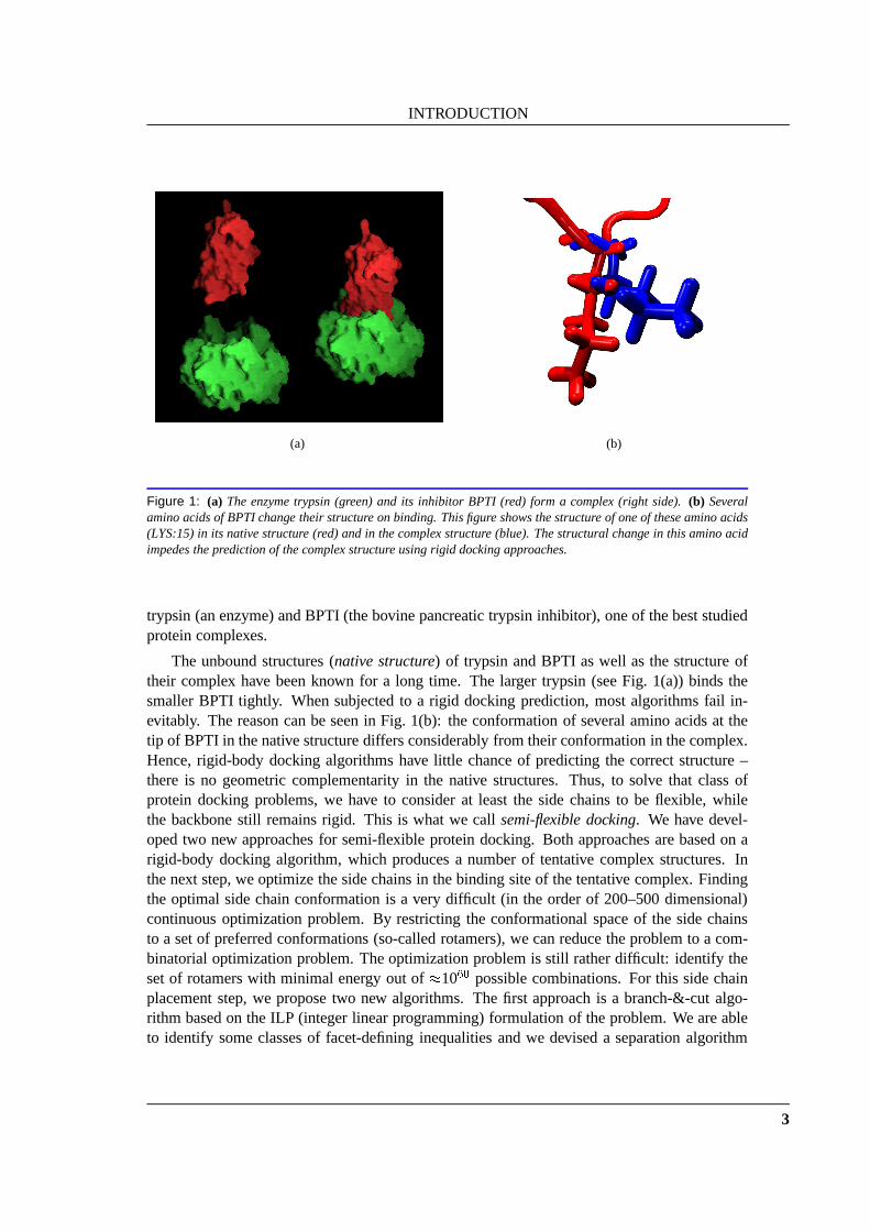
Figure 1: (a) The enzyme trypsin (green) and its inhibitor BPTI (red) forma complex (right side).(b) Severalamino acids of BPTI change their structure on binding. This figure shows the structure of one of these amino acids(LYS:15) in its native structure (red) and in the complex structure (blue). The structural change in this amino acidimpedes the prediction of the complex structure using rigiddocking approaches.
trypsin (an enzyme) and BPTI (the bovine pancreatic trypsininhibitor), one of the best studiedprotein complexes.
The unbound structures (native structure) of trypsin and BPTI as well as the structure oftheir complex have been known for a long time. The larger trypsin (see Fig. 1(a)) binds thesmaller BPTI tightly. When subjected to a rigid docking prediction, most algorithms fail in-evitably. The reason can be seen in Fig. 1(b): the conformation of several amino acids at thetip of BPTI in the native structure differs considerably from their conformation in the complex.Hence, rigid-body docking algorithms have little chance ofpredicting the correct structure –there is no geometric complementarity in the native structures. Thus, to solve that class ofprotein docking problems, we have to consider at least the side chains to be flexible, whilethe backbone still remains rigid. This is what we callsemi-flexible docking. We have devel-oped two new approaches for semi-flexible protein docking. Both approaches are based on arigid-body docking algorithm, which produces a number of tentative complex structures. Inthe next step, we optimize the side chains in the binding siteof the tentative complex. Findingthe optimal side chain conformation is a very difficult (in the order of 200–500 dimensional)continuous optimization problem. By restricting the conformational space of the side chainsto a set of preferred conformations (so-called rotamers), we can reduce the problem to a com-binatorial optimization problem. The optimization problem is still rather difficult: identify theset of rotamers with minimal energy out of�1060 possible combinations. For this side chainplacement step, we propose two new algorithms. The first approach is a branch-&-cut algo-rithm based on the ILP (integer linear programming) formulation of the problem. We are ableto identify some classes of facet-defining inequalities andwe devised a separation algorithm
3

INTRODUCTION
for a subclass of inequalities. The second approach is a fast, simple greedy approach. In con-trast to the branch-&-cut algorithm, the greedy approach yields usually suboptimal solutions.Nevertheless, both approaches were able to demangle the side chains of a test set of protease-inhibitor complexes. A final energetic evaluation of the demangled conformations correctlypredicts the true complex structure. After a short introduction to protein docking in general(Chapter 2), we describe these approaches for semi-flexibledocking in detail in Chapter 3.
Another major problem in protein docking is the accurate prediction of the binding free en-ergy of tentative complex structures, which is usually the basis for the final ranking performedby the docking algorithm. Although considerable progress has been made with the predictionof the binding free energy, it remains largely an unsolved problem. We develop a novel scor-ing function for protein-protein docking that is based on the integration of experimental data.This scoring function ranks the tentative complex structures with respect to the deviation of thepredicted nuclear magnetic resonance spectrum (NMR spectrum) from the experimental spec-trum. Since NMR spectra (especially the proton-NMR spectrawe use in this work) are easilyaccessible for protein complexes, the use of experimental data can improve the quality of dock-ing predictions significantly and can be used to assess the reliability of the results. We developtechniques for the prediction of NMR chemical shifts, the reconstruction of NMR spectra fromthe shift data, and for spectra comparison. This novel approach is the first docking approachthat permits the direct integration of experimental data into the docking algorithm. Its appli-cation to a set of protein-protein and protein-peptide complexes gives very promising results.Using this new technique, we can also solve a very difficult example of a protein-peptide com-plex, where all energy-based scoring functions fail. The methods and techniques developed forNMR-based docking are described in depth in Chapter 4 after ashort general introduction toNMR spectroscopy.
Rapid Software Prototyping
While developing new methods in protein docking as well as inother areas of ComputationalMolecular Biology, the most time-consuming step is the implementation. A major portion ofthis time is spent on the implementation of fundamental datastructures and algorithms. Thedata structures and algorithms are usually reimplemented again and again; code reuse is notvery common. We illustrate the main reasons for this with an example. In the course of ourprotein docking project, we experimented with advanced methods for energetic evaluations.One of these methods [54] consists of two major calculation steps: the calculation of the elec-trostatic contributions and the calculation of the molecular surface. Both methods are standardtechniques that were developed about 15 years ago and several implementations exist. We thenbought a commercially available software package for the electrostatic calculations and choseone of the freely available implementations for the molecular surface area calculation. Bothprograms were written in FORTRAN 77, the most common language for this kind of software.The integration of subroutines or major code portions from these two implementations into acommon program proved to be nearly impossible, since no thought was spent on reusabilitywhen designing the software. Furthermore, the lack of documentation or even comments inconjunction with FORTRAN-specific coding habits (e.g., one- or two-letter variable names)tends to turn even minor changes into a nightmare.
4

INTRODUCTION
The only means of integration we found was to implement rather large amounts of so-called “glue code”. This code had to convert the input data tothe specific file formats requiredby the two different programs. Although both programs basically used the PDB format to readatom coordinates, they required two different variants of the format which were incompatibleto each other. In the end, we implemented several hundred lines of code just to make bothprograms read standard PDB files. The extraction of the results from the (text-based) output ofthe programs again required rather complex code to gather all relevant numbers and ensure thatthe code really had correctly terminated. The resulting collection of interacting C programs,FORTRAN programs, and shell scripts was even less maintainable and less comprehensiblethan the original FORTRAN code.
We then looked at several large molecular modeling packages. The producers of thesepackages usually promise a good integration of several standard components. Often, there arealso software development kits (SDKs) available for the extension of existing methods and theintegration of new methods. But even these incredibly expensive packages have major draw-backs. Some of these packages are just nice graphical front ends to the very same FORTRANpackages mentioned above; they are basically glue code withwindows. The SDKs have ex-clusively procedural interfaces. We could not find any object-oriented approaches, which werepreferable with respect to reusability and extensibility of the code. Besides SDKs, many pack-ages also provide scripting languages that can be used to implement additional functionality.However, each package defines its own cryptic language, which often enough lacks even basiccontrol structures, so these approaches are seldom satisfactory.
There are also some (academic) efforts to create class libraries and frameworks in the fieldof Computational Molecular Modeling. Some prominent examples are PDBLib [18] (a libraryfor processing PDB files) and SCL [118]. These libraries havesome promising features, butnone of the existing libraries could provide us with sufficiently broad functionality.
Finally, there is is small number of scripting language extensions for Molecular Modelingand Computational Molecular Biology.BioPerl [12] andBioPython[13] are two projects thatstarted rather recently and do not yet provide any functionality in the field of Molecular Mod-eling. The software package that came closest to meeting ourneeds isMMTK, theMolecularModeling Toolkit. MMTK is an extension package for the object-oriented scripting languagePython [121] and provides some basic functionality for Molecular Modeling and visualization.Due to its object-oriented concept, MMTK is open and extensible on the scripting languagelevel. The time-critical sections of the code are implemented in C, resulting in good perfor-mance, but hindering reuse. Hence, the main drawbacks of MMTK are its limited functionalityand extensibility. Nevertheless, this package demonstrates the advantages of an object-orientedscripting language.
Our experience with these software packages led us to recognize the need for an extensi-ble, efficient, and object-oriented tool kit in the field of Molecular Modeling, which we thenstarted to implement. During the four years of its implementation, this tool set quickly evolvedinto something larger: it became a framework for rapid application development in MolecularModeling – BALL, the Biochemical Algorithms Library.
BALL is a large and powerful framework for rapid software prototyping written in C++.We use state-of-the-art software engineering techniques to ensure a thorough design and highcode quality. The resulting code is portable, robust, efficient, and extensible. Especially its
5

INTRODUCTION
extensibility, which results from an object-oriented and generic programming approach, distin-guishes BALL from all other software packages.
BALL provides an extensive set of data structures as well as classes for molecular me-chanics, advanced solvation methods, comparison and analysis of protein structures, file im-port/export, and visualization. To reduce turn-around times while developing new methods, weadded Python bindings for the majority of the BALL classes. Using the scripting language, it iseasier to inspect the data structures interactively. Additionally, the code can be modified at runtime without time-consuming compile or link stages. Once the Python code works as expected,it is very simple to port the Python code to C++. We have proven the rapid software prototyp-ing capabilities of BALL for a number of example applications in the field of protein dockingand protein engineering. The new techniques for protein docking described in the first part ofthis work have been implemented in BALL as well. Already the alpha release of BALL hasbeen successfully emplyed in about a dozen laboratories worldwide. The Max Planck Societyhonored the development of BALL with the Heinz Billing Award2000 for the Advancementof Scientific Computation.
Structure of the thesis
Following this introduction, Part II describes the new techniques for protein docking. First,we will give a short introduction to the biochemical concepts used in this work in Chapter 1.Chapter 2 gives an overview of protein docking and previous work in this field. We then presenttwo algorithms for semi-flexible docking in Chapter 3 and an algorithm for NMR-based proteindocking in Chapter 4. This part closes with a discussion of the presented docking algorithmsin Chapter 5.
The design and the implementation of BALL is then described in Part III. Chapter 6 de-scribes the architecture, design, and implementation of BALL. The techniques we used tomanage the project and to ensure software quality are presented in Chapter 7. An exampleapplication, which illustrates the rapid software prototyping capabilities of BALL and its ad-vantages over existing software, is given in Chapter 8. Chapter 9 discusses the current statusof BALL and points out some developments planned for the future.
This work then concludes with a discussion in Part IV.
6

Part II
Protein Docking

8
Chapter 1
Biochemistry – the Basics
This section gives an introduction to the biochemical termsused in this work. Since a seriousintroduction to this topic is beyond the scope of this work, we will just introduce the most im-portant terms and refer to biochemistry textbooks for a morecomplete coverage of the subject(e.g.[74, 114]).
1.1 Atoms and Molecules
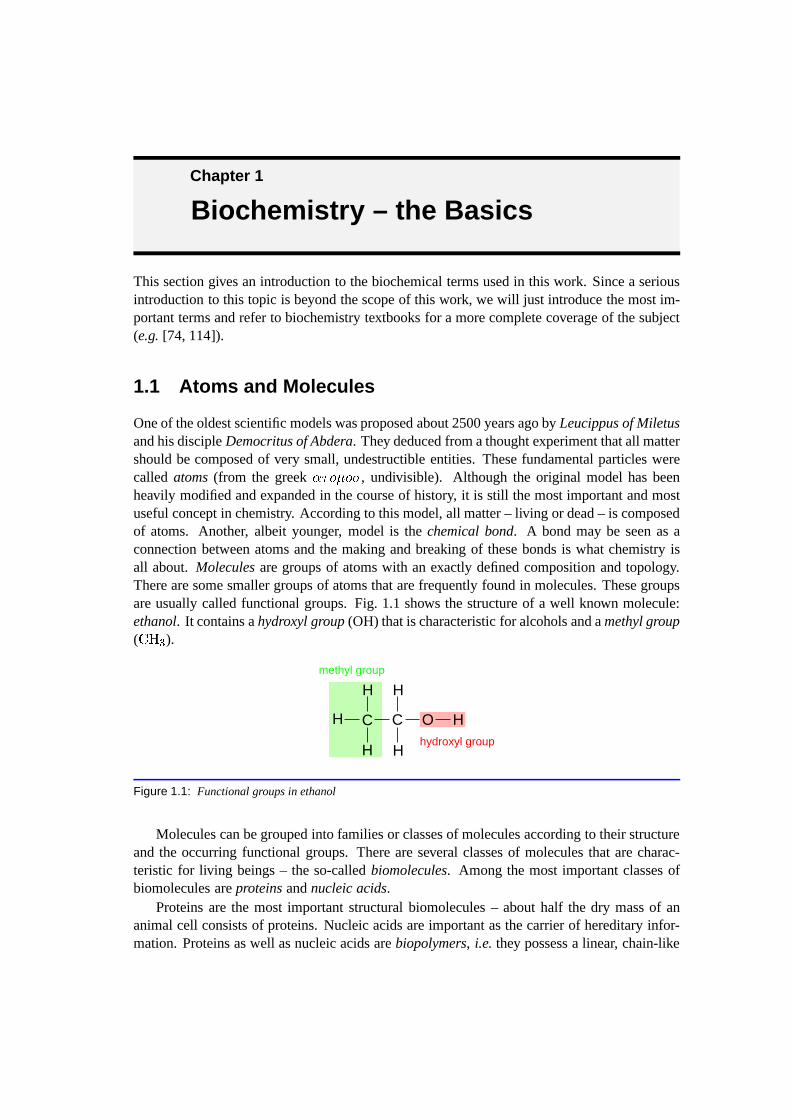
One of the oldest scientific models was proposed about 2500 years ago byLeucippus of Miletusand his discipleDemocritus of Abdera. They deduced from a thought experiment that all mattershould be composed of very small, undestructible entities.These fundamental particles werecalled atoms(from the greek��o�o�, undivisible). Although the original model has beenheavily modified and expanded in the course of history, it is still the most important and mostuseful concept in chemistry. According to this model, all matter – living or dead – is composedof atoms. Another, albeit younger, model is thechemical bond. A bond may be seen as aconnection between atoms and the making and breaking of these bonds is what chemistry isall about. Moleculesare groups of atoms with an exactly defined composition and topology.There are some smaller groups of atoms that are frequently found in molecules. These groupsare usually called functional groups. Fig. 1.1 shows the structure of a well known molecule:ethanol. It contains ahydroxyl group(OH) that is characteristic for alcohols and amethyl group(CH3).
C C
HH
H
H H
Ohydroxyl group
methyl group
H
Figure 1.1: Functional groups in ethanol
Molecules can be grouped into families or classes of molecules according to their structureand the occurring functional groups. There are several classes of molecules that are charac-teristic for living beings – the so-calledbiomolecules. Among the most important classes ofbiomolecules areproteinsandnucleic acids.
Proteins are the most important structural biomolecules – about half the dry mass of ananimal cell consists of proteins. Nucleic acids are important as the carrier of hereditary infor-mation. Proteins as well as nucleic acids arebiopolymers, i.e. they possess a linear, chain-like
CHAPTER 1. BIOCHEMISTRY – THE BASICS
structure. These chains are built from similar building blocks, themonomers. For proteins,these monomers are theamino acids.
1.2 Amino Acids
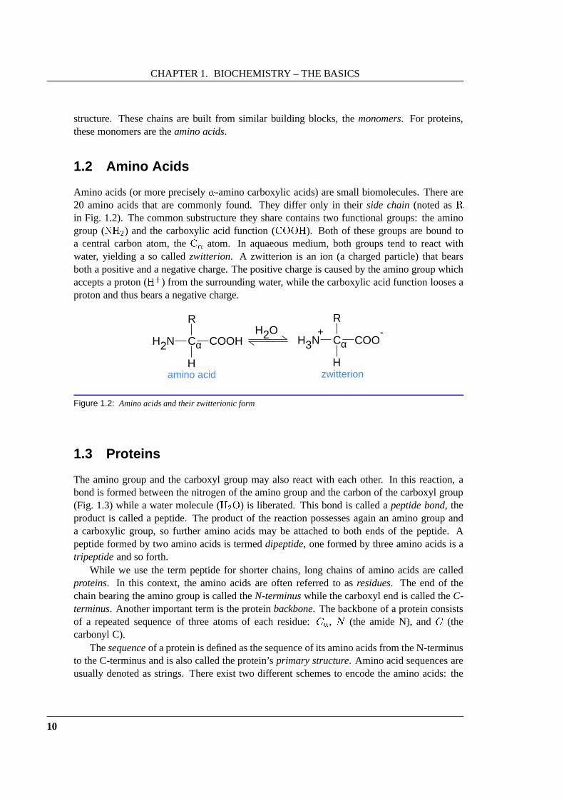
Amino acids (or more precisely�-amino carboxylic acids) are small biomolecules. There are20 amino acids that are commonly found. They differ only in their side chain(noted asRin Fig. 1.2). The common substructure they share contains two functional groups: the aminogroup (NH2) and the carboxylic acid function (COOH). Both of these groups are bound toa central carbon atom, theC� atom. In aquaeous medium, both groups tend to react withwater, yielding a so calledzwitterion. A zwitterion is an ion (a charged particle) that bearsboth a positive and a negative charge. The positive charge iscaused by the amino group whichaccepts a proton (H+) from the surrounding water, while the carboxylic acid function looses aproton and thus bears a negative charge.
H O2C
H
R
H N COOH2 α C
H
R
H N COO3 α+ -
amino acid zwitterion
Figure 1.2: Amino acids and their zwitterionic form
1.3 Proteins
The amino group and the carboxyl group may also react with each other. In this reaction, abond is formed between the nitrogen of the amino group and thecarbon of the carboxyl group(Fig. 1.3) while a water molecule (H2O) is liberated. This bond is called apeptide bond, theproduct is called a peptide. The product of the reaction possesses again an amino group anda carboxylic group, so further amino acids may be attached toboth ends of the peptide. Apeptide formed by two amino acids is termeddipeptide, one formed by three amino acids is atripeptideand so forth.
While we use the term peptide for shorter chains, long chainsof amino acids are calledproteins. In this context, the amino acids are often referred to asresidues. The end of thechain bearing the amino group is called theN-terminuswhile the carboxyl end is called theC-terminus. Another important term is the proteinbackbone. The backbone of a protein consistsof a repeated sequence of three atoms of each residue:C�, N (the amide N), andC (thecarbonyl C).
Thesequenceof a protein is defined as the sequence of its amino acids from the N-terminusto the C-terminus and is also called the protein’sprimary structure. Amino acid sequences areusually denoted as strings. There exist two different schemes to encode the amino acids: the
10

1.3. PROTEINS
C
H
R
H N COO3 α+ -
1
C
H
R
H N COO3 α+ -
2
+ C
H
R
H N C3 α+
1
O
C
H
R
COOα-
2
N
H
amino acid A amino acid B dipeptide
-H O2
Figure 1.3: The formation of a peptide bond
three-letter codewhich denotes each amino acid with three letters and the shorter but lesscomprehensibleone-letter code. In Fig. 1.5 an example for a protein sequence is shown.
Proteins also formsecondary structures. This term refers to certain spatially repeatingstructures found in proteins. There are two types of secondary structures: the�-helix and the�-pleated sheet. �-sheets are formed by parallel (or antiparallel) polypeptide chains (Fig. 1.4)that are bound to each other by hydrogen bonds between the backbone atoms.
Figure 1.4: A �-sheet is formed by two parallel polypeptide chains. They are often drawn as bands with arrowheads. For clarity, only the backbone of the two chains is shown.
An �-helix is a tight and regular helix of a polypeptide chain (Fig. 1.6). As in the�-sheet,this structure is stabilized by hydrogen bonds between backbone atoms. For a helix, thesehydrogen bonds are not between different chains but betweenresidues of the same chain. Thehelices are usually right-handed, although a left-handed variant exists as well.
Different sections of a protein chain may assume different secondary structures. The overallthree-dimensional structure (fold) of a single protein chain (including all its secondary structureelements) is termedtertiary structure.
Proteins often aggregate to larger structures. With multiple polypeptide chains,quarternarystructureis their interconnections and organization. The hierarchyof structures encountered ina large protein is shown in Fig. 1.5 on page 12.
11

CHAPTER 1. BIOCHEMISTRY – THE BASICS
VAL LEU SER PRO ALA ASP LYS THR ASN TRP ... TYR ARGprimary structure
helix sheetsecondary structure
tertiary structure
quarternary structure
Figure 1.5: The hierarchy of protein structures. Theprimary structureis defined as the amino acid sequence ofthe protein. Segments of a polypeptide chain may formsecondary structure elements: helices or sheets. The totalthree-dimensional structure of a protein is termedtertiary structure. Finally, several proteins may aggregate to formquarternary structures.
12
1.4. NUCLEIC ACIDS
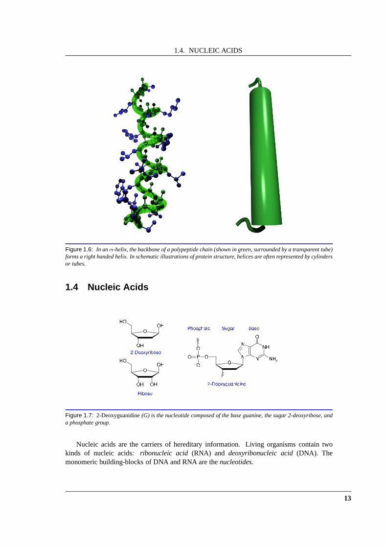
Figure 1.6: In an�-helix, the backbone of a polypeptide chain (shown in green,surrounded by a transparent tube)forms a right handed helix. In schematic illustrations of protein structure, helices are often represented by cylindersor tubes.
1.4 Nucleic Acids
Figure 1.7: 2-Deoxyguanidine(G) is the nucleotide composed of the base guanine, the sugar2-deoxyribose, anda phosphate group.
Nucleic acids are the carriers of hereditary information. Living organisms contain twokinds of nucleic acids: ribonucleic acid (RNA) and deoxyribonucleic acid(DNA). Themonomeric building-blocks of DNA and RNA are thenucleotides.
13
CHAPTER 1. BIOCHEMISTRY – THE BASICS
A nucleotide consists of three subunits: asugar, a phosphate, and abase. Fig. 1.7 showsthis structure as well as the two occurring sugars:ribosewhich occurs in RNA anddeoxyriboseoccurring in DNA.
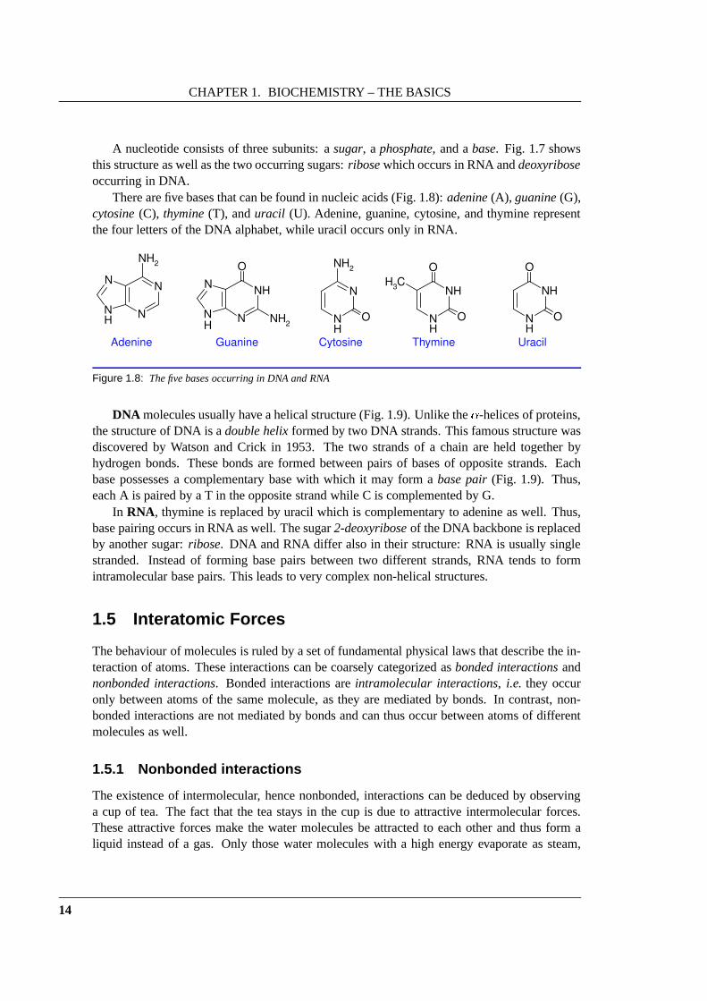
There are five bases that can be found in nucleic acids (Fig. 1.8): adenine(A), guanine(G),cytosine(C), thymine(T), anduracil (U). Adenine, guanine, cytosine, and thymine representthe four letters of the DNA alphabet, while uracil occurs only in RNA.
N H
N
N
N N H 2
O
H N
N
O
N H 2
H
N
N
N
N
N H 2
H N
N H
O
O
C H 3
H Thymine Adenine Cytosine Guanine
N
N H
O
O H
Uracil
Figure 1.8: The five bases occurring in DNA and RNA
DNA molecules usually have a helical structure (Fig. 1.9). Unlike the�-helices of proteins,the structure of DNA is adouble helixformed by two DNA strands. This famous structure wasdiscovered by Watson and Crick in 1953. The two strands of a chain are held together byhydrogen bonds. These bonds are formed between pairs of bases of opposite strands. Eachbase possesses a complementary base with which it may form abase pair(Fig. 1.9). Thus,each A is paired by a T in the opposite strand while C is complemented by G.
In RNA, thymine is replaced by uracil which is complementary to adenine as well. Thus,base pairing occurs in RNA as well. The sugar2-deoxyriboseof the DNA backbone is replacedby another sugar:ribose. DNA and RNA differ also in their structure: RNA is usually singlestranded. Instead of forming base pairs between two different strands, RNA tends to formintramolecular base pairs. This leads to very complex non-helical structures.
1.5 Interatomic Forces
The behaviour of molecules is ruled by a set of fundamental physical laws that describe the in-teraction of atoms. These interactions can be coarsely categorized asbonded interactionsandnonbonded interactions. Bonded interactions areintramolecular interactions, i.e. they occuronly between atoms of the same molecule, as they are mediatedby bonds. In contrast, non-bonded interactions are not mediated by bonds and can thus occur between atoms of differentmolecules as well.
1.5.1 Nonbonded interactions
The existence of intermolecular, hence nonbonded, interactions can be deduced by observinga cup of tea. The fact that the tea stays in the cup is due to attractive intermolecular forces.These attractive forces make the water molecules be attracted to each other and thus form aliquid instead of a gas. Only those water molecules with a high energy evaporate as steam,
14

1.5. INTERATOMIC FORCES
3' 5'
5'3'
C G
A T
G C
T A
T A
A T
N
N
N
N
NH2
H
ThymineAdenine
N
NH
O
CH3
H
N
N
N
N NH2
O
H
NN
O
NH2
H
CytosineGuanine
H
Figure 1.9: Double-stranded DNA assumes the structure of a double helix. The structure is stabilized by pairs ofcomplementary bases. These pairs form two (A-T) or three (C-G) hydrogen bonds.
as they contain a sufficient amount of energy to overcome the attractive interactions. Not allintermolecular forces are attractive. The fact that water has a well defined volume and is noteasily compressed is due to repulsive interactions that prevent the molecules from coming tooclose to each other.
Electrostatic interactions
One of the most important nonbonded interactions are the electrostatic interactions, whichoccur between electrostatic charges. Atoms consist of charged elementary particles (protonsand electrons). Protons bear a positive charge, while the electrons bear a negative charge ofequal magnitude. If atoms or molecules contain a different number of electrons and protons,they are calledions and they bear a positive or negative net charge. But also molecules withequal numbers of protons and electrons may still have a charge distribution that leads to so-called partial charges, i.e. regions of positive or negative charge excess. The interaction of
15

CHAPTER 1. BIOCHEMISTRY – THE BASICS
these electrostatic charges can be described byCoulomb’s law:EES = 14�"0 q1q2r (1.1)
whereEES is the energy resulting from the electrostatic interactionof two chargesq1 andq2with distancer between the charges."0 is the permittivity of the vacuum, a constant. Since theforcebetween the charges can be derived from the energy as the negative gradient, we can alsocalculate the forces between the two charges:~FES = �rEES (1.2)= � 14�"0 q1q2r3 ~r (1.3)
Depending on the sign of the chargesq1 andq2, electrostatic forces can be either attractive(opposite signs of the charges) or repulsive (same sign).
Van der Waals interactions
The termvan der Waals interactionsdescribes nonbonded interactions that consist of an at-tractive and a repulsive part. The attractive part stems form induced dipole–induced dipoleinteractions,i.e. fluctuations of the charge distribution in one atom or molecule induce chargefluctuations in a neighboring atom. These charge fluctuations lead to an attractive electrostaticinteraction. The repulsive part results form thepauli exclusion principle, a quantum mechan-ical effect that results in unfavorable energies for interpenetrating electron coulds of two ap-proaching atoms. The interplay of attractive and repulsiveinteractions leads to intermolecularpotential functions like that shown in Fig. 1.10. For large distances, the energy approacheszero. At intermediate distances, the energy is negative, which leads to attractive forces. Ifthe distance between the atoms is further reduced, the repulsive forces grow rapidly and givehighly positive energies. There are different models to describe that kind of potential. Themost commonly used expression uses two parametersA andB that depend of the type of theatoms involved to describe the van der Waals energy as a function of the atom distancer:EvdW = Ar12 � Br6 (1.4)
1.5.2 Molecular Mechanics
Molecular Mechanics is an approach based on simple physicalmodels of molecular and atomicinteractions. The parameters of these models are usually obtained by fitting to experimentaldata. The resulting set of equations describing the interactions and the corresponding param-eters are called aforce field. Besides the nonbonded interactions described in the previoussection, the force fields also include bonded interactions,which can be modeled in a numberof different ways.
16

1.5. INTERATOMIC FORCES
0E
r
Figure 1.10: The distance dependence of the van der Waals energy.
A typical force field like the AMBER force field defines the total energy of a set ofmolecules as the sum of five different types of interactions:Etotal = EvdW +EES +Ebend +Estret h +Etorsion=Xi<j Aijr12ij � Bijr6ij !+ 14�"0 Xi<j qiqjrij+ X(i;j)2bonds kstret hij (rij � r0ij)2+ Xa2angles kbenda (�a � �0a)2+ Xb2torsions ktorsionb (1 + os(nb�b � �0b))The van der Waals energyEvdW and theelectrostatic energyEES are the nonbonded inter-
actions. Thestretch energyEstret h describes the change in the energy as the bond distancerij varies. This energy is described by a harmonic potential (i.e. a quadratic function of thedeviation from the optimal bond distance, see Fig. 1.11). Similarly, the bend energyEbenddescribes the variation of the energy with the bond angle� formed by two neighboring bonds.This contribution is also described by a harmonic potential. The contributionEtorsion describesthetorsion energy. Torsions describe the variation of the total energy on rotation about a bond.The torsion energy depends on thetorsion angle�. It is defined as the angle that is enclosedby the two planes defined by atoms(i; j; k) and(j; k; l) (see Fig. 1.11). The variation of theenergy with this angle can be described as a cosine function.
17

CHAPTER 1. BIOCHEMISTRY – THE BASICS
stretch bend torsion
ri jij
i j
k
θ
φ
i
jk
l
Figure 1.11: The bonded interactions in a typical Molecular Mechanics force field.
This form of the force field describes the energy as a functionof the coordinates. For manyapplications it is also necessary to know the forces caused by these interactions. The force~Fiacting upon atomi may be derived as the negative gradient of the energy:~Fi = �rE = �rEvdW �rEES �rEstret h �rEbend �rEtorsion (1.5)
The force field permits the calculation of the static and dynamic properties of molecules orsets of molecules. There are numerous applications for force fields. Among the most impor-tant ones are energy minimization and Molecular Dynamics simulations. Energy minimizationmeans to search for the molecular geometry with the lowest energy, a very difficult multi-dimensional optimization problem that is usually tackled using gradient-based optimizationtechniques. Molecular Dynamics is based on the fact that theforce field gives a full descriptionof the forces acting upon the atoms. If these forces can be calculated for arbitrary geome-tries, one can apply Newton’s equations of motion and thus simulate the dynamic behaviour ofmolecules.
18

Chapter 2
Introduction
Since the protein docking problem was already introduced inPart I, we will only briefly repeatthe problem definition here: We are given the three-dimensional structure of two proteinsAandB, that are known to form a complexAB. The protein docking problem is then to predictthe structure of the complexAB.
The protein docking problem has numerous interesting applications. Besides the standardproblem (how does the complex structure look like?), it may also speed up the time-consumingprocess of structure elucidation (see Chapter 4). The results of docking predictions are alsouseful for the analysis and the understanding of the bindingmodes of proteins and numerousnew applications will arise with the coming advent of Proteomics. The following sections willbriefly discuss existing approaches for protein docking, their limitations, and some possibilitiesfor improvement.
2.1 Rigid Body Docking
Rigid protein protein docking is based on a rather old analogy by German chemist Emil Fischer,the so-calledlock-and-key principlehe proposed in 1894:\Invertin und Emulsin haben bekanntli h man he Aehnli hkeit mit denProte��nsto�en und besitzen wie jene unzweifelhaft ein asymmetris h gebautesMolek�ul. Ihre bes hr�ankte Wirkung auf die Glu oside liesse si h also au h dur hdie Annahme erkl�aren, dass nur bei �ahnli hem geometris hem Bau diejenigeAnn�aherung der Molek�ule statt�nden kann, wel he zur Ausl�osung des hemis henVorganges erforderli h ist. Um ein Bild zu gebrauchen, will ich sagen, dass Enzym
und Glucosid wie Schloss und Schlussel zu einander passen mussen, um eine hemi-s he Wirkung aufeinander aus�uben zu k�onnen. 1" [34], p. 2992
This model implies that enzyme and substrate (or in our case:the two proteins) are rigid bodiesthat possess regions of geometric complementarity. A contemporary view of this model isshown in Fig. 2.1. In the mean time, the lock-and-key model has been superceded by a numberof various other models,e.g.the induced fithypothesis by David Koshland [64]. However, itis still of fundamental importance and for many protein-protein interactions it remains a validassumption, as has been shown in a recent study by Betts and Sternberg [11].
The first docking algorithms were based on the assumptions ofrigidity and complementar-ity (thus the namerigid-body docking, RBD). They tried to identify geometrically complemen-tary sections of the proteinsA andB. These regions should define the binding site of the com-
1English translation: “Invertin and emulsin are known to share some similarities with protein compounds and,like those, possess an asymmetric molecular structure. Their limited effect on glycosides could thus be explainedby the hypothesis that the approachment that is necessary toinitiate the chemical process is only possible if themolecules are geometrically similar to each other.To use an image, I would say that enzyme and glycoside haveto fit into each other like a lock and a key, in order to exert a chemical effect on each other.”

CHAPTER 2. INTRODUCTION
Figure 2.1: Paul Ehrlich applied Fischer’s lock-and-key principle to immunoreactions. He illustrated his notionof the concept in this drawing from 1900 [29].
plex. For example, the correlation-based techniques introduced by Katchalski-Katziret al.[60]estimate the contact area ofA andB and assign those structures with the largest contact areathe best scores. These purely geometric algorithms (e.g.[20, 125, 33, 32]) were successful fora large number of examples.
It was soon recognized, that geometric complementarity alone is not sufficient to identifythe binding site. The next generation of algorithms thus employed simple energy functionsto estimate the binding free energy of the resulting complexes. These energy functions usu-ally consider only a part of the physics involved in the binding process,e.g.only electrostaticinteractions [40, 119] or hydrogen bonds [80].
Today, most RBD algorithms share a similar overall structure (Fig. 2.2, page 22). In a firststep, a large number of potential complex structures is created from the two protein structuresA andB. This generation step is usually based on geometric complementarity. For example,in the algorithm by Lenhof [70], this structure generation is based on the matching of trianglesof surface points ofA and triangles formed by atom centers ofB. A pair of triangles fromAandB matches, if the side lengths of the triangles coincide within a certain tolerance. Each of
20

2.2. DOCKING AND PROTEIN FLEXIBILITY
these triangle pairs defines a rigid transformation that bringsB into close contact withA. Thisstructure generation step can be implemented very efficiently using geometric hashing tech-niques and can produce huge amounts of tentative complex structures in a short time (usuallyseveral thousands). In the vast majority of cases, this set of candidates contains a number ofgood approximations of the true complex structure (where “good” means that the RMSD2 ofall atoms is below3 A).
The next (and clearly the most difficult) task is the identification of these good approxi-mations among the candidates. We will refer to them astrue positives, while the remainingstructures (those that do not resemble the true complex structure) will be calledfalse positives.Numerous methods have been proposed to distinguish true positives from false positives. Inprinciple, it were sufficient to calculate the binding free energy of each of the tentative complexstructures, as the true positives should possess the lowestbinding free energy. However, this isa non-trivial task, since only very rough approximations are known to estimate the free energyon binding.
A large number of other scoring functions have been tested for the protein docking problem,but the correct prediction of binding free energies is stillone of the most difficult problems inthis field. We cannot enumerate all these methods, so we referto the comprehensive review bySternberget al. [113].
In all algorithms, one or more of these scoring functions areapplied to the initial set ofcandidates. The output of each docking algorithm is thus a ranked list of structures, where thegood approximations should be at the top of the list (bottom of Fig. 2.2). If the generation stepproduced good approximations of the true complex structures and the scoring function wereideal, one should expect that the candidate with the best score were a good approximation ofthe true complex structure. One measure of the algorithm’s quality is thus the rank assigned tothe first true positive in the list.
2.2 Docking and Protein Flexibility
RBD algorithms perform rather well as long as the structure of the two proteins does not changesignificantly upon complex formation. Unfortunately, there are numerous examples where thisassumption does not hold. They are explained with Koshland’s induced fithypothesis, whichbasically states that the two partners change their shape upon binding and form a complexstructure where they possess geometric complementarity. In contrast to the lock-and-key prin-ciple, the induced fit hypothesis does not require the unbound structures ofA andB to displaygeometric complementarity. Clearly, this leads to a more difficult docking problem. Thoseexamples that show structural changes on binding fall essentially into two categories:� domain movements� side chain movements
2root mean square deviation
21

CHAPTER 2. INTRODUCTION
Filtering
Final Energetic Evaluation
Structure Generation
A B
< <
Figure 2.2: The overall structure of a rigid-body docking algorithm.
22

2.3. COMBINING NMR DATA AND DOCKING ALGORITHMS
Domain movements
In the first case, large rigid sections of the protein (domains) move around “hinges”, flexiblejoints tethering the domains and restricting their movement. The hinges are formed by smallregions of high backbone flexibility, while the backbone remains essentially rigid inside thedomains. In the case of domain movements, one of the major difficulties is to distinguishbetween rigid and flexible parts of the protein. Also the total number of hinges that can beconsidered is usually very limited due to the number of degrees of freedom associated witheach hinge. One way to handle domain movements was proposed by Sandaket al. [105, 106].Their algorithms performs a search of the full three-dimensional rotational space of a hingebetween two domains. To identify the best structure, a number of potential hinge locations istested and a geometric docking is carried out. Finally, all structures resulting from all possiblehinge positions are ranked with respect to geometric complementarity.
Side chain flexibility
In the second and more frequent case, the protein backbone remains essentially rigid, butside chains undergo conformational changes on binding. An example for this category is thecomplex of trypsin and BPTI, as we have already discussed in Part I (page 2). Norelet al. [89]studied the bound and unbound structures of 26 protein complexes and could show thatthe protein backbones remain rigid upon binding and only theside chains show significantconformational changes for the majority of all examples.
RBD approaches have little hope for success if domain or sidechain movements occur.This is mainly due to the fact that the two unbound structures(which represent the input of thedocking algorithm) do not possess the geometric complementarity the bound structures have.Even though the initial candidate set often contains a largenumber of true positives, they areusually not ranked correctly. The failure of the scoring functions stems from the fact that sidechains ofA andB overlap for many true positives. The resulting structures cannot occur innature, they are physically meaningless. Hence, the scoring functions are not able to give areasonable estimate of the true binding energy.
Several approaches have been proposed to overcome these difficulties. Common to theseapproaches is an intermediate stage, where the side chain conformations of the initial candi-dates are demangled to produce physically meaningful structures. In Chapter 3 we present twonew approaches to protein docking with flexible side chains.The first technique uses a greedyheuristic to place the side chains, while the second approach is a branch-&-cut algorithm thatyields optimal solutions to the side chain placement problem.
2.3 Combining NMR Data and Docking Algorithms
Since it is not yet possible to predict the free energies on binding with sufficient accuracy, otherways have to be found to increase the reliability of the docking results. This can be done bycounterchecking the results against experimental data. This experimental data should be easilyaccessible and should allow a ranking of the docking resultsor at least some way of validation.
23

CHAPTER 2. INTRODUCTION
Nuclear Magnetic Resonance (NMR) spectroscopy is one of thetwo important methodsof protein structure elucidation. It provides data that contains a large amount of structural in-formation. This information has been used in ligand dockingfor quite some time to predictthe structure of protein-ligand complexes [127, 44, 98]. With the fundamentals of NMR spec-troscopy being discussed in depth in Chapter 4, we will only briefly explain these methodshere. There are different kinds of structural information available from NMR data. The eas-iest to obtain are simpleNMR spectra. These spectra measure the so-calledchemical shift,an intrinsic property of each atom of the protein. This shiftdepends on the structural envi-ronment (electronic surrounding, geometry, neighboring atoms,etc.) of the atom, hence thevalue of the chemical shift contains structural information. However, due to the large numberof atoms showing in such a spectrum (typically several hundreds), it is a non-trivial task todecide which of the peaks in the spectrum belongs to which atom. This task is also calledshiftassignmentand is the most time-consuming task in NMR-based structure elucidation, whichcan often take several months. All of the above mentioned protein-ligand docking methods arebased on fully assigned spectra. From these spectra, geometric constraints (NOE3 constraints)are derived. The methods are then based upon the integrationof these distance constraints intoexisting docking techniques and the resulting structures have to satisfy as many of these con-straints as possible. A similar methodology was recently proposed by Morelliet al. [82] forprotein-protein docking. They used NOE constraints in a soft docking algorithm to predict thestructure of the complex of cytochrome 553 and ferredoxin.
In contrast to these constraint-based docking methods, ouralgorithm does not require ashift assignment. This extends the applicability of the method to use structures where no NMRshift assignment is known (e.g.structures determined by X-ray methods). Furthermore, weonly need an unassigned1H-NMR spectrum of the complex, which is the simplest kind ofspectrum and thus easy and cheap to obtain. Instead of processing the spectra (which has yetto be done manually) and extracting geometric information from the experimental data, wechose the opposite approach. We process the candidates generated from a RBD algorithm andpredict their spectra. These spectra are then compared to the experimental spectrum and rankedaccording to their similarity. Hence, no prior processing and evaluation of the experimentaldata is required. Chapter 4 gives a short introduction to thebasics of NMR spectroscopy andthen explains our new approach in more detail.
3NOE – nuclear Overhauser effect. This effect permits the estimation of the distance betweenneighboringatoms.
24

Chapter 3
Semi-Flexible Docking
3.1 Introduction
The previous chapter introduced the basic techniques for rigid body protein docking and theirlimitations. Since completely flexible protein docking is computationally very expensive,the use of flexible side chains is a reasonable compromise. Wecall the docking with rigidbackbones and flexible side chainssemi-flexible docking. Algorithms for semi-flexible dockingare similar to the algorithms for rigid-body docking. They introduce an additional step, theside chain demangling. In this step, the side chain orientations in the binding site of eachtentative complex structure are optimized and occurring overlaps are thus removed. Thisdemangling step ensures physically meaningful structuresthat are then subjected to a finalenergetic evaluation and ranking. The next sections will first discuss existing techniquesfor side chain placement and then we will describe our new approaches and some resultsobtained with these techniques. Parts of this chapter have been previously published in [2, 3, 4].
Figure 3.1: This figure illustrates torsion angles in an amino acid side chain. The torsion angles determine therotation about single bonds in the side chain. The first two torsion angles in a side chain are usually denoted�1and�2.
First, we have to define what side chain flexibility means. In principle, theN atoms ofa side chain have3N translational degrees of freedom. In protein structures, we usually ob-serve that bond lengths and bond angles deviate only slightly from the ideal values observedin structures of minimal energy. The reason is that the energy needed to stretch a bond ordeform a bond angle is much larger than the energy required toperform rotations around the
CHAPTER 3. SEMI-FLEXIBLE DOCKING
bond. Therefore, the side chain’s main source of flexibilityare torsions around single bonds(see Fig. 3.1). A side chain has a small number of these torsional degrees of freedom (betweenzero and five torsion angles depending on the amino acid). Restricting side chain flexibility totorsional flexibility drastically cuts down the complexityof the side chain placement problem.
In 1987, Ponder and Richards [99] observed that the side chain conformations occurringin proteins can be adequately described by a rather small setof so-calledrotamersfor eachamino acid. Fig. 3.2 shows a so calledRamachandran plot. It was obtained by examininga set of known protein structures. For each lysine side chainoccurring in the structure, thefirst two side chain torsion angles�1 and�2 were determined. The plot shows the observedfrequency of these angles. Obviously, not all possible angle combinations are assumed withequal probability. In fact, there are only three small and well-defined regions whose anglecombinations occur frequently in proteins. These regions are small enough to assume thatthe conformations in a region are energetically equivalent. Therefore, Ponder and Richardsargued that it is sufficient to describe the conformational space of a side chain through a set ofconformations, the so-called rotamers. In our example, therotamers would correspond to theconformation obtained by picking the three maxima in the Ramachandran plot. All rotamersof the amino acid side chains form a so-calledrotamer library.
The use of the rotamer representation for the side chain conformations reduces the initialcontinuous optimization problem to a discrete combinatorial optimization problem: we have toidentify the set of rotamers with the minimum energy,i.e. theglobal minimum energy confor-mation(GMEC).
In principle, each side chain can assume any of its rotamers,hence the total number ofcombinations is the product of the number of rotamers for each side chain. With the typicalnumber of side chains in a binding site ranging from 40 to 60, the total number of possiblerotamer combinations can become as high as1060 combinations. Thus, efficient algorithms arerequired to identify the GMEC or suboptimal solutions sufficiently close to the GMEC.
Side chain placement has been discussed in depth not only forthe ab initio prediction ofprotein structures and homology modeling. There is a wide range of techniques available forside chain placement. Due to the high dimensionality of the conformational space of all sidechains, exhaustive search is only tractable for a very smallnumber of side chains [16, 128].Other approaches use Monte Carlo methods [1, 50], local homology modeling [65], or self-consistent field theory [62] to place the side chains.
Methods for side chain demangling were also successfully applied to protein docking.Totrov and Abagyan [117] used a Monte Carlo approach to predict the structure of a lysozyme-antibody complex. Wenget al. [128] optimized the side chains in the binding site of threeprotease-inhibitor complexes using exhaustive search. Jacksonet al. [53] employed a self-consistent mean field approach and a Langevin dipole model for the side chain placement inseveral protein complexes.
However, no algorithm has been yet presented that employs anoptimal side chain place-ment for the interface refinement in protein-protein docking except for the exhaustive search ofWenget al. [128], which is severely limited in the number of side chainsand thus not tractablefor larger protein interfaces.
The only algorithm that is able to solve the side chain placement problem to optimality for arelated problem (protein-ligand docking) was proposed by Leach [67, 69]. Leach first employs
26

3.1. INTRODUCTION
0 50 100 150 200 250 300 3500
50
100
150
200
250
300
350
Frequency [a.u.]
χ1 [deg]
χ 2 [deg
]
1.000
1.583
2.167
2.750
3.333
3.917
4.500
5.083
5.667
6.250
6.833
7.417
8.000
Figure 3.2: Ramachandran plot for the�1 and�2 torsion angles of LYS. The color coding represents the frequencyof occurrence in a protein test set in arbitrary units.
the Dead End Elimination theorem to reduce the complexity ofthe placement problem andthen the A* algorithm to determine an optimal placement of the side chains of the receptorwith respect to a Molecular Mechanics force field.
We present two new techniques for protein interface refinement and their application tothe docking of unbound protein structures. First, we present a fast heuristic that usually yieldssuboptimal solutions to the side chain placement problem. Nevertheless, the solution is closeenough to the optimal solution to allow the correct prediction of the true complex structures fora test set of unbound protein structures. Second, we proposethe first algorithm that allows theoptimal, albeit slower, demangling of side chains of large protein interfaces. This method isbased on the formulation of the side chain placement problemas an integer linear program andits solution using a branch-&-cut algorithm. The results ofexperiments with three protease-inhibitor complexes are presented in Section 3.3.
27

CHAPTER 3. SEMI-FLEXIBLE DOCKING
3.2 The Docking Algorithm
The input of the docking algorithm consists of two proteinsA andB in their unbound confor-mation. These proteins are subjected to a rigid docking, yielding a set of candidate conforma-tions. For the 60 best candidates out of this set, we perform aside chain demangling. Finally,the candidates are scored according to their binding free energy.
3.2.1 Rigid Docking
A rigid docking is performed for the proteinsA andB, using an improved version of the algo-rithm described in [70] and [71]. The algorithm uses geometric complementarity and simplechemical fitness functions to create a large set of potentialcomplex structures. Out of this set,the 60 best candidates with respect to geometric complementarity are selected. An experimentwith a test set of docking structures (35 complexes) always produced several good approxima-tions of the true complex structure among the 60 best candidates.
3.2.2 Side Chain Demangling
The rigid docking algorithm, which generates a set of promising candidates, neglects the sidechain flexibility. Therefore, many of the candidates have strong overlaps and incorrectly placedside chains. In order to obtain physically meaningful conformations, we have to demangle theside chains of the protein interface (the binding site).
Determination of the binding site
First, we have to identify all residues ofA andB that belong to the binding site. We considera residue to be part of the binding site if any of its atoms is within 6 A of any atom of the otherprotein. All residues that fulfill this condition are markedand kept in a listBS. Side chainswithout rotamers (CYS engaged in disulfide bonds, ALA, and GLY) are excluded from thislist. For each residue in this list, we determine its set of possible rotamers from the rotamerlibrary of Dunbracket al. [28], assuming that the side chain can occur only in one of theseconformations. We have now decomposed the protein residuesinto two disjoint sets: one setcomprises all residues that have rotamers and belong to the binding site as defined by our cutoff criterion, and the other set comprises all remaining residues (= the template).
Decomposition of the total energy
The GMEC is now defined as the combination of rotamers yielding the lowest total energy. Thisentails a combinatorial optimization problem where we mustsearch a huge conformationalspace for the GMEC. In order to demangle the side chains of thebinding site, we have toidentify the GMEC or a good approximation thereof. By the following decomposition we canexpress the total energy of the system as a function of the selected rotamers:Etotal = Etpl +Xi Etplir +Xi Xj<i Epwir ;js (3.1)
28

3.2. THE DOCKING ALGORITHM
whereEtpl is the potential energy of the template (= system without residues of the bindingsite) andEtplir is the potential energy of side chaini in rotameric stater (short: rotamerir)interacting with the atoms of the template (including the internal energy ofir). Epwir ;js is thepairwise potential energy between side chaini in rotameric stater and side chainj in ro-tameric states. This decomposition is exact, as the AMBER force field contains only pairwisenonbonded interactions. Since rotamers that heavily overlap with the rigid template cannot bepart of the GMEC, we remove all rotamers whose interaction energy with the template is largerthan100 kJ=mol.
For a given set of rotamers, the single energy components of eq 3.1 can be easily calculatedvia the Molecular Mechanics force field. The computational effort required for the evaluationscales at most quadratically with the number of atoms (thereare at mostN2 nonbonded atompairs forN atoms). The difficulty arises in finding the global minimum asthis means pickingthe optimal combination of rotamers for the side chains. Fortunately, the search space can besignificantly reduced by the so-calleddead-end elimination theorem(DEE)[25], which can bestated as follows: if for a pair of rotamers(ir; it),Etplir +Xj 6=i mins Epwir ;js > Etplit +Xj 6=i maxs Epwit ;js (3.2)
holds, then the rotamerir can be safely ignored in the search for the global minimum. Itera-tively applying the DEE theorem reduces the number of combinations of rotamers by severalorders of magnitude (see also the table in Section 3.3 on page40).
Search of minimum energy conformation
In order to find an optimal combination of rotamers, we have developed two alternative ap-proaches: a tree-based multi-greedy (MG) method and abranch-&-cut algorithmbased onan ILP (Integer Linear Programming) formulation of our problem. We will first describe thegreedy method and then explain the more technical branch-&-cut algorithm.
3.2.3 The Multi-Greedy Method
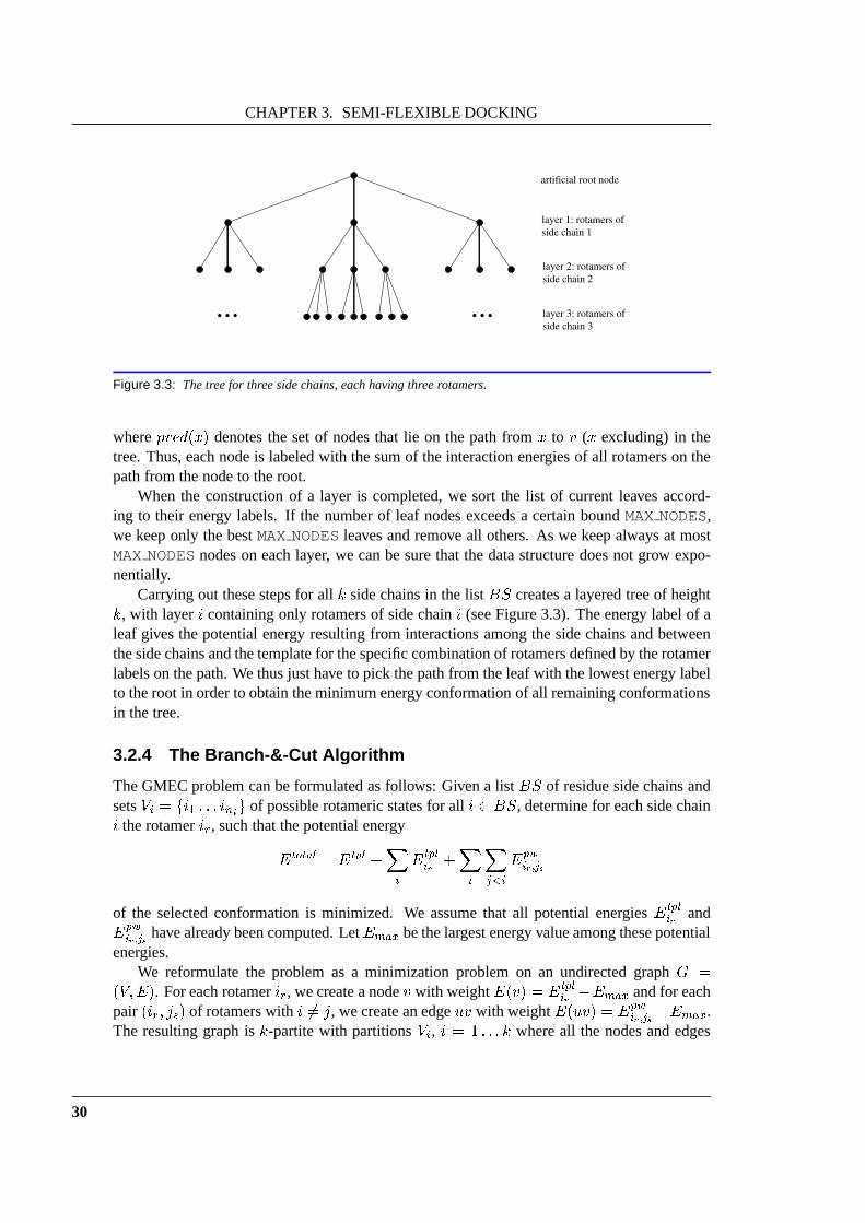
In this approach, an enumeration tree representing all possible rotamer combinations is built.The tree consists ofk = jBSj layers, each representing one side chain. Each path from theroot to a leaf represents a possible combination of rotamers. The label of the node in layeridetermines which rotamer is selected for side chaini. Every node also possesses an energylabel. For the construction, we start out with an artificial root nodev, which is given an energylabelE(v) = Etpl and a rotamer labelr(v) = null. For each side chaini, we add a newlayer to the tree. This layer is constructed by adding a node for each rotamer ofi to each leafof the previous layer (see Figure 3.3). Each new nodex for a rotameris is labeled with thecorresponding rotamer (r(x) = is) and its energy label is set toE(x) = Etplis +E(parent (x)) + Xy2pred(x)Epwis ;r(y);
29
CHAPTER 3. SEMI-FLEXIBLE DOCKING
... ...
layer 1: rotamers of
side chain 1
layer 2: rotamers of
side chain 2
layer 3: rotamers of
side chain 3
artificial root node
Figure 3.3: The tree for three side chains, each having three rotamers.
wherepred(x) denotes the set of nodes that lie on the path fromx to v (x excluding) in thetree. Thus, each node is labeled with the sum of the interaction energies of all rotamers on thepath from the node to the root.
When the construction of a layer is completed, we sort the list of current leaves accord-ing to their energy labels. If the number of leaf nodes exceeds a certain boundMAXNODES,we keep only the bestMAXNODESleaves and remove all others. As we keep always at mostMAXNODESnodes on each layer, we can be sure that the data structure does not grow expo-nentially.
Carrying out these steps for allk side chains in the listBS creates a layered tree of heightk, with layeri containing only rotamers of side chaini (see Figure 3.3). The energy label of aleaf gives the potential energy resulting from interactions among the side chains and betweenthe side chains and the template for the specific combinationof rotamers defined by the rotamerlabels on the path. We thus just have to pick the path from the leaf with the lowest energy labelto the root in order to obtain the minimum energy conformation of all remaining conformationsin the tree.
3.2.4 The Branch-&-Cut Algorithm
The GMEC problem can be formulated as follows: Given a listBS of residue side chains andsetsVi = fi1 : : : inig of possible rotameric states for alli 2 BS, determine for each side chaini the rotamerir, such that the potential energyEtotal = Etpl +Xi Etplir +Xi Xj<i Epwir ;jsof the selected conformation is minimized. We assume that all potential energiesEtplir andEpwir ;js have already been computed. LetEmax be the largest energy value among these potentialenergies.
We reformulate the problem as a minimization problem on an undirected graphG =(V;E). For each rotamerir, we create a nodev with weightE(v) = Etplir �Emax and for eachpair (ir; js) of rotamers withi 6= j, we create an edgeuv with weightE(uv) = Epwir ;js �Emax.The resulting graph isk-partite with partitionsVi, i = 1 : : : k where all the nodes and edges
30

3.2. THE DOCKING ALGORITHM
have negative weights. The partitionVi is called thei-th column of the graph. For a nodev ofthe graph, we define (v) to be the column of this node. The possible rotamer sets correspondto the subgraphs ofG with the following property: Every subgraph consists of exactly k nodes,one node out of each column, and the induced edges. We call these subgraphsrotamer graphs.The weight of a rotamer graph is the sum of the weights of its nodes and edges. Note thatthe weight of a rotamer graph and the energy of its corresponding rotamer combination differexactly byEtpl + (k + �k2�) � Emax. Thus, the GMEC problem can be solved by determiningthe rotamer graph ofG with minimal weight.
The Integer Linear Program
We now transform this graph-theoretic description into an integer linear program by introduc-ing a binary decision variablexv for each nodev andxuv for each edgeuv. If a node (edge)belongs to the rotamer graph, the value of the variablexv (xuv) is 1 and otherwise it is0. Forbrevity, we say that a node or an edge is selected if the corresponding binary decision variableis 1. The basic constraint system of the GMEC problem is the following:min Xv2V E(v)xv + Xuv2EE(uv)xuv!s:t: Xv2Vi xv = 1 for all i 2 f1 : : : kg (3.3)xuv � xv for all uv 2 E (3.4)xuv � xu for all uv 2 E (3.5)xv 2 f0; 1g for all v 2 V (3.6)xuv 2 f0; 1g for all uv 2 E (3.7)
The constraints (3.3) enforce that exactly one node of each partition, i.e. exactly one ro-tamer for each side chain, is selected. The constraints (3.4) and (3.5) guarantee that an edge canonly be selected if both endpoints are selected,i.e. we include the pairwise interaction energybetween two rotamers only if both rotamers are selected as well. Since only one edge from acertain columni to a nodev can be selected, we can tighten these inequalities toXu2Vi xuv � xv for all v 2 V , i 6= (v): (3.8)
Note that the above integer linear program has subgraphs of rotamer graphs as feasible solu-tions. Of course, the weight of a complete rotamer graph is smaller than the weight of any ofits subgraphs, so that the optimal solution of the integer linear program is a rotamer graph.
Branch-&-Cut
Branch-&-cut is the most common technique to handle hard combinatorial optimization prob-lems. It works as follows: We relax the integer linear program by dropping the integralitycondition and solve the resulting linear program. If the solution �x is integral we have the opti-mal solution. Otherwise, we search for a valid inequalityfx � f0 that cuts off the solution�x,
31
CHAPTER 3. SEMI-FLEXIBLE DOCKING
i.e. fy � f0 for all feasible solutionsy andf �x > f0; the setfx j fx = f0g is called a cuttingplane. The search for the cutting plane is called the separation problem. Any cutting planefound is added to the linear program and the linear program isresolved. The generation of cut-ting planes is repeated until either an optimal solution is found or the search for a cutting planefails. In the second case a branch step follows: We generate two subproblems by setting onefractional variablexv (xuv) to 0 in the first subproblem and to1 in the second subproblem andsolve these subproblems recursively. This gives rise to an enumeration tree of subproblems.
For details about branch-&-cut, integer programming, and adiscussion of improvementson this method, see the book of Wolsey [131].
The GMEC polyhedron
We call the convex hullP of all feasible solutions theGMEC polyhedron. Since its facets arethe most promising cutting planes, we studied the structureof the GMEC polyhedron. Beforewe can prove that an inequality defines a facet, we have to determine the dimension of thepolyhedron. We assume that the reader is familiar with polyhedral theory; for an introduction,see [87, 131].Definition: A polyhedronP � Rn is the set of points that satisfies a finite number of linearinequalities. Every polyhedronP can be written asP = fx 2 Rn j Ax � dg for somem�n-matrixA and somem-vectord. Note that this description of a polyhedron is not unique. For i,1 � i � m letAi be thei-th row ofA. If Aix = di for somex 2 Rn the constraintAix � diis calledactive for x. Let M be the set of indices, so thati 2 M if and only if Aix � di isactive for allx 2 P . Furthermore, let(A=; d=) be the corresponding rows of(A; d). In otherwords,A=x � d= are the constraints ofAx � d which hold with equality for all points of thepolyhedron.
Lemma 1. dim(P ) = jV j � k + jEjProof. A fundamental lemma about polyhedral theory (see, for example, [87], page 87) statesthat dim(P ) + rank(A=; d=) = jV j+ jEj;where rank(A=; d=) is the number of linearly independent rows of(A=; d=). Note thatrank(A=; d=) is independent of the particular description ofP .
Hence,dim(P ) � jV j � k+ jEj, because we havek linearly independent equalities in ourpartial description of the polyhedron. In order to show thatdim(P ) � jV j � k + jEj, we haveto show that there arejV j � k + jEj + 1 affinely independent feasible solutions.
A basic solutionb is a feasible solution withbuv = 0 for all uv 2 E. For i, 1 � i � kwe defineb(i) to be the nodev of Vi with bv = 1. For any nodev let ev be the unit vector ofthis node,i.e. the vector with entry1 at the position ofv and with entry0 at all other positions.Analogously for any edgeuv, let euv be the unit vector of this edge. For an0=1-vectorx wedo not distinguish between the vector and the correspondingsubgraph.
Let b be a basic solution. We then construct all solutions where exactly one node ofb isreplaced by another one in the same column. Additionally, weconstruct one solution for every
32

3.2. THE DOCKING ALGORITHM
edge by including the edge, both its endpoints. For the remaining columns, we take the nodesof the basic solutionb. More formally, we look at the following setS of feasible solutions:S = fbg [ fb+ ev � eb( (v)) j v 2 V with bv = 0g[ fb+ euv + eu � eb( (u)) + ev � eb( (v)) j uv 2 EgThe size of the set is1 + jV j � k + jEj. LetM be the matrix with rows corresponding to thesolutions ofS. We have to show that the solutions are affinely independent,i.e. if one subtractsone row ofM from the others, the remaining rows are linear independent.In this case, thematrix has to have full row rank. We denote then � n identity matrix byIn. We subtractbfrom all other solutions and get the matrixM 0 with rowsev�eb( (v)) for all v 2 V with bv = 0and rowseuv + eu � eb( (u)) + ev � eb( (v)) for all uv 2 E. Since dropping columns cannotincrease the row rank of the matrix, we are allowed to drop allcolumnsi of M 0 with bi = 1, i.e.all columns that have an entry�1. This results in a matrix with the following block-structure� IjV j�k 0B IjEj �for some suitable matrixB. This matrix has full rank since it is triangular. Thus, the matrixM 0 has full row rank and all solutions ofS are affinely independent.
Lemma 2. The non-negativity constraintsxuv � 0 define facets for alluv 2 E. The one-node-aggregation constraints (3.8) define facets forP .
Proof. A feasible constraint defines a facet, if it is active forjV j�k+ jEj affinely independentsolutions.
For the first part, we have to show thatxuv = 0 for jV j � k + jEj affinely independentsolutions. This is obvious, because all but one of the solutions in the proof of Lemma 1 satisfythis equality. The second part follows if we choose a basic solution b with bv = 0. ThenPu2Vi xuv = xv for all but one selected solutions.
Definition: Leth; i; j be pairwise distinct column indices,(S1; S2) be a partition ofVi, (T1; T2)be a partition ofVj and(R1; R2) be a partition ofVh. Furthermore, all sets are assumed to benon-empty. We define the edge-incompatibility constraint for S1; S2; T1; T2; R1; R2 asXu2S2;v2T1 xuv+ Xv2T2;w2R1 xvw+ Xw2R2;u2S1 xuw � 1 (3.9)
Lemma 3. The edge-incompatibility constraints are feasible forP and define facets.
Proof. We first show the feasibility of the constraint. If any edge ofthe constraint is selected,no other edge of the constraint can be selected, because at least one of its endpoints cannot beselected (see Fig. 3.4).
In order to prove that the constraints are facet-defining, weuse an indirect way to show thatthere arejV j � k + jEj affinely independent solutions for which the constraint is active.
33

CHAPTER 3. SEMI-FLEXIBLE DOCKING
S
S
T
T
R
R
2
1
1
2
2
1
Figure 3.4: Only one of these edges can be selected.
LetF = fp1; : : : ptg be the set of feasible solutions for which the constraint (3.9) is active.The constraint defines a facet if all solutions(�; �0) of the set of equalitiesXv2V �vpiv + Xuv2E �uvpiuv = �0 for all pi 2 F (3.10)
are linear combinations of the coefficients of the constraint (3.9) and the feasible equationsA=x = b= of the problem (see Theorem 3.6. in Chapter I of [87]),i.e.(�; �0) = (�pj + �A=; �+ �b=) for all pj 2 FThe set of feasible equations consists ofk equations of the formXv2Vi xv = 1 (3.11)
i.e., one equation for each partitionVi. The scalar factor for the equation of columnVi in thelinear combination is denoted by�i, the scalar factor of the constraint (3.9) is denoted by�.The above cited theorem implies that constraint (3.9) is facet-defining if� �v = �i for each nodev 2 Vi (becausepjv = 0 for all pj 2 F; v 2 V )� �uv = � for each edgeuv in constraint (3.9)� �uv = 0 for all other edges� �0 = �+Pki=1 �i.Let b be a basic solution. We call a constraintXv2V �vxv + Xuv2E �uvxuv = �0 (3.12)
34

3.2. THE DOCKING ALGORITHM
in normal form with respect tob if �v = 0 for all v with bv = 1. By subtracting the equations(3.11) multiplied with suitable factors, it is possible to transform each constraint into (at least)one equivalent constraint in normal form with respect tob.
Thus, a constraint of type (3.9) defines a facet ofP if all solutions of the equation systemXv2V �vpiv + Xuv2E �uvpiuv = �0 for all pi 2 F�v = 0 for all v with bv = 1 (3.13)
are of the form� �v = �i for each nodev 2 Vi� �uv = � for each edgeuv in constraint (3.9)� �uv = 0 for all other edges� �0 = �+Pki=1 �i.Since every columnVi contains one nodev with �v = 0 (normal form), the above equationscan only be fulfilled if all�i are zero. Therefore, we have to show that�v = 0 for each nodev 2 Vi, �uv = � for each edgeuv in constraint (3.9),�uv = 0 for all other edges, and�0 = �.
Choose any basic solutionb, such that at least one edgexy of the constraint is selectable,i.e. bx = 1 andby = 1. Let F be the set of all feasible solutions where exactly one edge ofthe constraint is chosen. We first argue that�v = 0 for all nodesv 2 V . By definition of thenormal form, this is true for all nodes of the basic solution.Let v =2 Vh [ Vi [ Vj. Look atthe following two solutions: the nodes of the basic solutiontogether with the edgexy and thesolution wherev andb( (v)) are exchanged and the same edge is selected. More formally, welook at the solutionsb + exy andb+ exy + ev � eb( (v)). Since�b( (v)) = 0, the difference ofthe two resulting constraints is�v = 0. Now let v 2 Vh [ Vi [ Vj. Letwr be an edge of theconstraint that has neither endpoint in the same row asv. Take any solution where this edgeandb( (v)) are selected and the solution whereb( (v)) is replaced byv. Again the differencebetween the two constraints is�v = 0.
Now we conclude that�wr = �0 for all edgeswr in the constraint (look at any solutionwhere only this edge is selected), and that�wr = 0 for all edges not in the constraint (look atany solution where this edge and one edge of the constraint isselected and the solution whereonly the edge of the constraint is selected). This proves that all solutions of the equation system(3.13) have the required form and we are done.
Definition: Let h; i; j be pairwise distinct column indices,S � Vi, T � Vj with S; T 6= ;,and letR1; R2 be a partition ofVh with Ri 6= ; for i = 1; 2. We define the node-aggregationconstraints forS; T;R1; R2 asXu2S;v2T xuv + Xu2S;w2R1 xuw + Xv2T;w2R2 xvw �Xu2S xu +Xv2T xv (3.14)
35

CHAPTER 3. SEMI-FLEXIBLE DOCKING
2
S T
R
R 1
Figure 3.5: One can select only as many edges as nodes in the shaded sets.
Lemma 4. The node-aggregation constraints (3.14) are feasible forP and define facets.
Proof. Again we start with the feasibility proof. If a node inS, a node inT , and a node inR1are selected we can select exactly one edge going fromS to T and one edge going fromS toR1 but no edges fromT toR2. If a node inS is selected but no node inT we cannot select anedge fromS to T or fromT toR2. Furthermore, we can select at most one edge fromS toR1.If neither a node fromS nor a node fromT is selected, we cannot select any of the edges ofthe constraint. The other cases are analogous (compare Fig.3.5).
As in the proof of Lemma 3, we use Theorem 3.6. in Chapter I of [87] to show that theconstraints are facet-defining. LetF = fp1; : : : ptg be the set of feasible solutions that satisfythe constraint with equality. A constraint of type (3.14) defines a facet ofP if all solutions ofthe equation systemXv2V �vpiv + Xuv2E �uvpiuv = �0 for all pi 2 F�v = 0 for all v with bv = 1 (3.15)
are linear combinations of the coefficients of the node-aggregation constraints and the feasiblesolutions with scalar factors� and�i. Thus,(�;mu0) has to be of the form� �v = �i�� for each nodev 2 Vi; v 2 S[T (becausepjv = �1 for all v 2 S[T; pj 2 F )� �v = �i for each nodev 2 Vi; v =2 S [ T� �uv = � for each edgeuv in constraint (3.14)� �uv = 0 for all other edges� �0 = �+Pki=1 �i.
Choose any basic solutionb with bu = 0 for all u 2 S [ T . The constraint (3.14) is innormal form with respect tob. In a solution of this equation system,�v = 0 for all v 2 V withbv = 1.
36

3.2. THE DOCKING ALGORITHM
Furthermore,�v = �i for all v 2 V with bv = 1 by the choice of the basic solution andthus�i = 0 for all 1 � i � k.
Therefore, we have to show that�v = �� for each nodev 2 S [ T , �v = 0 for each nodev =2 S [ T , �uv = � for each edgeuv in constraint (3.14),�uv = 0 for all other edges, and�0 = �.Letw be the node inVh with bw = 1 and w.l.o.g. assumew 2 R1 andr is any node ofR2.
Since the constraint is active forb we conclude that�0 = 0. Furthermore, we obtain:
1. �v = 0 for all v 2 V that are not in the constraint (look at the difference between theconstraints for the solutionsb andb+ ev � eb( (v))).
2. �uv = 0 for all uv 2 E that are not in the constraint (look at the difference between theconstraint of any active solutionp with puv = 1 andp� euv).
3. �u = ��uv for all u 2 S, v 2 R1 (look at the difference between the constraints ofb+ ev � eb( (v)) andb+ ev � eb( (v)) + eu � eb( (u)) + euv).4. �u = ��uv for all u 2 T , v 2 R2 (The same argument).
5. �v = ��uv for all u 2 S, v 2 T (look at the difference between the constraints for thesolutionsb+ eu � eb( (u)) + euw andb+ eu � eb( (v)) + euw + ev � eb( (v)) + euv).
6. �u = ��uv for all u 2 S, v 2 T (look at the difference betweenthe constraints for the solutionsb + ev � eb( (v)) + er � ew + erv andb+ ev � eb( (v)) + er � ew + erv + eu � eb( (u)) + euv).
Thus, for allu 2 S[T andv 2 V such that the edgeuv is in the constraint, we have shownthat�u = ��uv. Since the subgraph induced by the constraint is connected,all �v have thesame value. Choose� = ��v for a nodev of the constraint. Then,�uv = ��v = � for eachedgeuv of the constraint. Hence, all solutions of the equation system (3.13) have the requiredform and we are done.
We have implemented a branch-&-cut algorithm for the GMEC problem using the C++class library LEDA [78], ABACUS [59] for the administrationof the branch-&-cut tree, andCPLEX [52] to solve the linear programs.
We use the node-summation equations (3.3) and the one-node-aggregation constraints (3.8)as the initial constraint system. The only constraints thatare separated are the node-aggregationconstraints (3.14) withjSj = jT j = 1.
We use a simple, brute force algorithm. We iterate over all triples(u; v; h), whereu; v 2 V ,h is a column of the graphG and (u); (v); h are pairwise distinct. The optimal partition isobtained by iterating over the nodes ofVh and putting a nodew intoR1 if xuw > xvw and intoR2 otherwise.
37

CHAPTER 3. SEMI-FLEXIBLE DOCKING
The running time is O( kXi=1 kXj=1 kXh=1(jVijjVj jjVhj)) = O(jV j3):3.2.5 Energetic Evaluation
∆ intB-A
G
A-B
solute
∆∆GsolvA
∆∆GsolvB
int∆G
+
-
A
-
+
+
+
- -
+
+
-
- B
+
-
- B
++
+ -
-
+ - -
+
+
- B
A
++
- -
++
A
+
solvent
a b
c d
e
Figure 3.6: Calculation of the electrostatic contributions to the binding free energy.
After determining an optimal rotamer set for each candidate, we assign the rotamers of theminimum energy conformation to the respective side chains and then optimize the side chainsof the binding-site using the AMBER force field. The free energy of binding is determinedusing the method proposed by Jackson and Sternberg [54].
We decompose the binding free energy�Gass as follows:�Gass = �GES +�G av +�G onf +�GvdW (3.16)�GES represents the electrostatic contribution,�G av the cavitation free energy in water,�G onf the change in conformational entropy of the proteins, and�GvdW the change in thevan der Waals free energy.
Electrostatic contribution
The electrostatic contributions to the binding free energycan be estimated using a so-calledcontinuum model. This type of model considers solvent molecules not explicitly, but implicitas a spatial dependency of the dielectric constant. The solute is represented by a region of lowdielectric constant immersed in a high dielectric constantsolvent (water). The boundary be-tween these two regions is formed by the molecular surface ofthe solute (the solvent excludedsurface).
38
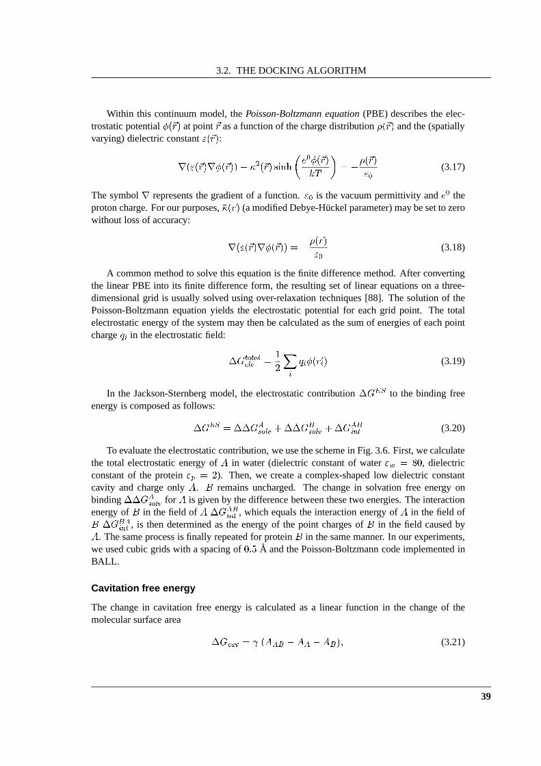
3.2. THE DOCKING ALGORITHM
Within this continuum model, thePoisson-Boltzmann equation(PBE) describes the elec-trostatic potential�(~r) at point~r as a function of the charge distribution�(~r) and the (spatiallyvarying) dielectric constant"(~r):r("(~r)r�(~r))� ��2(~r) sinh�e0�(~r)kT � = ��(~r)"0 (3.17)
The symbolr represents the gradient of a function."0 is the vacuum permittivity ande0 theproton charge. For our purposes,��(~r) (a modified Debye-Huckel parameter) may be set to zerowithout loss of accuracy: r("(~r)r�(~r)) = ��(~r)"0 (3.18)
A common method to solve this equation is the finite difference method. After convertingthe linear PBE into its finite difference form, the resultingset of linear equations on a three-dimensional grid is usually solved using over-relaxation techniques [88]. The solution of thePoisson-Boltzmann equation yields the electrostatic potential for each grid point. The totalelectrostatic energy of the system may then be calculated asthe sum of energies of each pointchargeqi in the electrostatic field:�Gtotalele = 12Xi qi�(~ri) (3.19)
In the Jackson-Sternberg model, the electrostatic contribution �GES to the binding freeenergy is composed as follows:�GES = ��GAsolv +��GBsolv +�GABint (3.20)
To evaluate the electrostatic contribution, we use the scheme in Fig. 3.6. First, we calculatethe total electrostatic energy ofA in water (dielectric constant of water"w = 80, dielectricconstant of the protein"p = 2). Then, we create a complex-shaped low dielectric constantcavity and charge onlyA. B remains uncharged. The change in solvation free energy onbinding��GAsolv for A is given by the difference between these two energies. The interactionenergy ofB in the field ofA �GABint , which equals the interaction energy ofA in the field ofB �GBAint , is then determined as the energy of the point charges ofB in the field caused byA. The same process is finally repeated for proteinB in the same manner. In our experiments,we used cubic grids with a spacing of0:5 A and the Poisson-Boltzmann code implemented inBALL.
Cavitation free energy
The change in cavitation free energy is calculated as a linear function in the change of themolecular surface area �G av = (AAB �AA �AB); (3.21)
39

CHAPTER 3. SEMI-FLEXIBLE DOCKING
whereAAB , AA, andAB are the molecular surface areas of the complex, proteinA, andproteinB, respectively, and is a constant (0:289 kJmol�1A�2
). We use the algorithm byConnolly [20] (as implemented in BALL) to calculate the molecular surface areas with a proberadius of1:4 A. For the electrostatic calculations, we use the PARSE set of atom radii andcharges by Sitkoffet al. [109] and the FDPB implementation of BALL.
3.3 Experimental Results
We applied our techniques to three protease-inhibitor complexes. The structures of three pro-teasesA and the corresponding protein inhibitorsB were taken from the PDB: subtilisin carls-berg (1SBC) with chymotrypsin inhibitor 2 (2CI2),�-trypsin (1TPO) with trypsin inhibitor(4PTI), and�-chymotrypsin A (5CHA, chain A) with ovomucoid (2OVO). Water was removedfrom each of these complexes, hydrogens were added and theirpositions were optimized usingthe AMBER [22] force field.
Combinatorial complexity
The iterative application of the DEE theorem reduced the combinatorial complexity usuallyby about ten orders of magnitude, thus greatly simplifying the solution of the GMEC problem.Numbers for the three examples are given in the following table:
complex no. of side # rotamer combinationschains before DEE after DEE
1TPO/4PTI 51 6 � 1060 8 � 10451SBC/2CI2 50 1 � 1055 2 � 1046
5CHA/2OVO 54 1 � 1056 2 � 1048Ranking of the structures
In the case of 1TPO/4PTI, the AMBER energy already gave a clear signal; the best four can-didates (those with lowest energy) were good approximations of the complex structure (seeFig. 3.7: structures are good approximations of the true complex structure if their RMSD1 islow). When ranking this example with respect to the estimated binding free energy (calculatedwith the Jackson-Sternberg model as described in Section 3.2), an approximation of the truecomplex structure was ranked as number one as well (see Fig. 3.8).
For the example 1SBC/2CI2, the AMBER energy was not sufficient to predict the truecomplex structure correctly. However, when ranked according to the binding free energy, thebest candidate was a good approximation of the true complex structure for all examples (seeFig. 3.9, 3.8, and 3.10).
We also tried to predict the structure of these examples using the binding free energy alone(i.e. without a prior side chain demangling). None of the complexes was correctly predicted.
1root mean square deviation of all atom position
40

3.3. EXPERIMENTAL RESULTS
0
10
20
30
40
50
60
-20000 -18000 -16000 -14000 -12000 -10000 -8000 -6000
RM
SD
[Ang
stro
m]
binding energy [kJ/mol]
Figure 3.7: 1TPO/4PTI - AMBER energy of the candidates (MG).
0
10
20
30
40
50
60
-300 -200 -100 0 100 200 300 400
RM
SD
[Ang
stro
m]
binding energy [kJ/mol]
Figure 3.8: 1TPO/4PTI - ranking of the candidates according to their binding free energy (MG).
Hence, side chain demangling as well as an advanced scoring method are both needed to predictthe correct complex structure in these cases.
41

CHAPTER 3. SEMI-FLEXIBLE DOCKING
0
10
20
30
40
50
60
70
-300 -200 -100 0 100 200 300
RM
SD
[Ang
stro
m]
binding energy [kJ/mol]
Figure 3.9: 1SBC/4CI2 - ranking of the candidates according to their binding free energy (MG).
0
10
20
30
40
50
60
-200 -100 0 100 200 300 400 500
RM
SD
[Ang
stro
m]
binding energy [kJ/mol]
Figure 3.10: 5CHA/2OVO - ranking of the candidates according to their binding free energy (MG).
Quality of the heuristic
For the case of 1TPO/4PTI, we checked the quality of the results obtained from the MG methodby calculating the optimal solution using the branch-&-cutalgorithm. We performed this cal-
42

3.3. EXPERIMENTAL RESULTS
culation for 34 out of the 60 candidates. In most cases, the solution found by the heuristicwas close to the optimal solution,i.e. for the majority of the side chains the selected rotamerswere identical to those of the optimal solution. The total energy differed only slightly fromthat of the optimal solution, hence the ranking was very similar to that of the optimal solution(see Figs. 3.7 and 3.11). The average error in the AMBER energies was about8000 kJ=mol.However, the quality of the solutions was better for good approximations of the true complexstructure. Among the 34 candidates considered, 7 were good approximations (RMSD� 4 A).Only one of these seven candidates was further than1000 kJ=mol away from the optimum.
Side chain placement
For the protein docking problem, not all side chains are of equal importance. However, theplacement of a single side chain may determine the success ofthe docking. A prominentexample is LYS:15 of 4PTI. When compared to the bound structure, this side chain has toturn towards the core of 1TPO to fit properly. Fig. 3.12 shows the bound and the unboundconformation of this side chain. However, it is not necessary for LYS:15 to assume the fullyextended position as in the complex structure, it just has toturn down a bit further than it doesin the unbound structure to avoid clashes with the backbone of 1TPO. Although the correctplacement of the side chain is not achieved, the selected rotamer is sufficient to allow a reliableprediction of the binding free energy.
Running times
We compared the running times of the different parts of our docking algorithm on a SUNEnterprise 10000 (333 MHz UltraSparc II processors, 12 GB RAM, Solaris 7, g++-2.95.2 with-O2). We averaged the running times for each stage of the algorithm over all 60 candidatesconsidered. Obviously, running time is dominated by the final energetic evaluation and theinitial calculation of the energetic contributions, whereas the side chain placement itself onlyaccounts for a minor portion of the total running time.
stage avg. time [min]
energies and DEE 30ILP 14multi-greedy 3side chain optimization 5final energetic evaluation (FDPB) 70
43
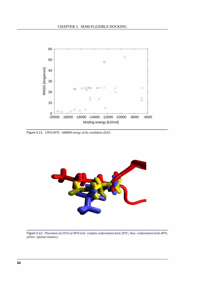
CHAPTER 3. SEMI-FLEXIBLE DOCKING
0
10
20
30
40
50
60
-20000 -18000 -16000 -14000 -12000 -10000 -8000 -6000
RM
SD
[Ang
stro
m]
binding energy [kJ/mol]
Figure 3.11: 1TPO/4PTI - AMBER energy of the candidates (ILP).
Figure 3.12: Placement of LYS15 of 4PTI (red: complex conformation from 2PTC, blue: conformation from 4PTI,yellow: optimal rotamer).
44

Chapter 4
Protein Docking and NMR
4.1 Nuclear Magnetic Resonance Spectroscopy
One of the most important tasks in structural biology is the determination of the three-dimensional structure of biomolecules. Currently, there are three methods that are frequentlyemployed in structure determination:X-ray crystallography, Nuclear Magnetic Resonance(NMR) spectroscopy, andelectron microscopy. While the latter of the three methods is ofminor importance and only yields low-resolution structures, X-ray crystallography and NMRspectroscopy are powerful tools to explore the structure ofbiomolecules at the atomic scale.
In X-ray crystallography, X-rays are focussed onto a protein crystal and the resultingdiffraction patterns are recorded. From these patterns, the structure of the protein can be recon-structed through aFourier transform. This technique is applicable to proteins of all sizes, theonly prerequisite being the ability to grow crystals of the protein in question.
The second technique, which we will discuss in more depth, isthe Nuclear Magnetic Res-onance spectroscopy. The development of NMR spectroscopy was initiated by the pioneeringwork of F. Bloch and E. M. Purcell in 1945 [14, 101]. During thefollowing decades, it becamethe method of choice for structure elucidation in organic chemistry. Due to new techniques andinstruments, the size of the molecules accessible to NMR spectroscopy grew constantly untilstructure determination became feasible for small to medium sized proteins.
There is a whole range of textbooks covering the fundamentals and advanced topics ofNMR spectroscopy (e.g.[48, 42, 120, 39, 45]), so we will just mention the fundamental physicsand discuss the details only insofar as they are essential tothe understanding of the subsequentsections.
4.1.1 The Nuclear Angular Momentum
NMR is based on the fact that the nuclei of most atoms possess anuclear angular momentumP , which, according to the classical picture, corresponds toa rotation of the nucleus about anaxis. From quantum mechanical considerations, one can deduce that the angular momentum ofsuch an isolated particle cannot assume arbitrary magnitudes but is quantized (i.e. it may onlytake certain discrete values). For the angular momentum, these values can be specified in termsof aquantum numberI: j~P j =pI(I + 1) ~; (4.1)
whereh = 2�~ is the Planck constant. Theangular momentum quantum number(or spinquantum number) I is determined by the nucleus,i.e. it is determined by the isotope of theelement (nuclide) in question. Nuclides with a spin quantum number ofI = 0 do not possessan angular momentum and are thus not accessible through NMR spectroscopy (see Table 4.1).

CHAPTER 4. PROTEIN DOCKING AND NMR
Nuclide Natural abundance Spin quantum number Gyromagnetic ratio[%] I [107radT�1s�1]1H 99:985 12 26:752H 0:015 1 4:1112C 98:9 0 �13C 1:108 12 6:7314N 99:63 1 1:9315N 0:37 12 �2:7116O 99:96 0 �17O 0:037 52 �3:63
Table 4.1: Magnetic properties of the most important nuclides (valuesfrom [39]).
Associated with the angular momentumP is themagnetic moment�:~� = ~P (4.2)
The gyromagnetic ratio is a constant specific to each nuclide. Both~� and ~P are vectorialproperties, so their full description requires a directionas well. When placed in a static mag-netic field ~B0 along the z-axis, the spins of the nuclei orient themselves along the field in away that their z-component is quantized as well:Pz = m~ with m = I; I � 1; I � 2; : : : � I (4.3)
wherem is themagnetic quantum number. Sincem can assume all values given in eq 4.3,Pz(and~�) can assume2I + 1 possibles values (see Fig. 4.1). Hence, the energy of the nucleus inthe magnetic field~B0 is quantized as well:E = ��zj ~B0 j = �m ~j ~B0 j (4.4)
From here on, we will consider only nuclei withI = 12 (e.g.1H) for the sake of simplicity.Similar considerations apply to the other nuclei as well.1H nuclei (protons), can assume twodifferent energy levels in accordance with the two possiblevalues of the magnetic quantumnumberm = +12 ;�12 . If �z is positive,~� is parallel to the external magnetic field, which isthe preferred orientation. Transitions between these two states can be caused by the transfer ofan appropriate amount of energy�E. This energy has to correspond to the difference of thetwo energy levels,i.e. �E = E+ 12 �E� 12 (4.4)= ~j ~B0 j: (4.5)
The energies required for this transition are comparatively small. For typical NMR instruments,they correspond to electromagnetic radiation with frequencies in the range of several MHz toseveral hundreds of MHz. This frequency is called theresonance frequencyof the nuclide.
46

4.1. NUCLEAR MAGNETIC RESONANCE SPECTROSCOPY
h2
-
B0
m = + 12
h2
+
12
m = -
z
x
y
Figure 4.1: Left: The nuclear angular momentum vector~P of a proton (1H ) can assume two different statesdefined by its magnetic quantum numberm. The z-component of the spin is either parallel or antiparallel to theexternal field~B0 . Right: Since this quantization condition holds only for the z-component, the spins may havearbitrary x- and z-components, i.e. they lie on cones definedby the total angular momentumP and its z-component.
According to the quantization condition (4.3), only the z-component is quantized. Classicalphysics require a magnetic moment in a field to perform a rotational movement around thez-axis which describes a cone (see Fig. 4.1). Such a movementis generally referred to asprecession(analogous to the motion of a gyroscope). In the case of NMR, it is known asLarmor precession. The angular velocity! of the precession and the correspondingLarmorfrequency� = !2� are proportional to the external field~B0 :� = j�Ejh = j ~jh j ~B0 j (4.6)= j j2� j ~B0 j (4.7)! = j jj ~B0 j (4.8)
4.1.2 Electronic Shielding and the Chemical Shift
From the equations stated above, one should expect all nuclei of a certain nuclide to show thesame energy difference�E for a given magnetic field. However, atoms also contain electronsand these cause a local magnetic field which is superposed to the external field. As a result,the nucleus is shielded from the external field and experiences only aneffective field~Be� . Theshielding is proportional to the external field and is therefore written in terms of theshieldingconstant���: ~Be� = ~B0 +� ~B = ~B0 � ��� ~B0 (4.9)
The shielding constant depends on the local environment (and thus on the molecular structure)of the nucleus in question. Since��� is a tensor quantity, the effective field depends on theorientation of the molecule relative to the magnetic field vector ~B0 . Hence, the random dis-tribution of this orientation in liquid samples causes the non-isotropic contributions of��� tovanish. The experiment only reveals the isotropic shielding constant� which is the trace of the
47

CHAPTER 4. PROTEIN DOCKING AND NMR
AB
C
x
y
z
CCD
E
B0
Figure 4.2: Basic components of an NMR spectrometer: The sample (A) is placed in a strong homogeneousmagnetic field~B0 caused by a magnet (B). The field can be modified using the sweepcoils (C). Radio pulses aretransmitted using the transmitter coils (D) and received via the receiver coils (E).
shielding tensor: � = 13(�xx + �yy + �zz) (4.10)
More practical than the shielding constant� is the chemical shifts scale (orÆ-scale). Thisscale describes the difference between the resonance frequencies of a given nucleus relative tothe resonance frequency of a reference compound:Æ = � � �ref�ref (4.11)Æ is named thechemical shiftand is usually given in units of ppm (parts per million,10�6). Thechemical shift of the reference compound is zero by definition. Although the chemical shift isalso a tensor quantity, we will regard it as a scalar quantityfor the reasons stated above for theshielding tensor.
4.1.3 The Basic NMR Experiment
Fig. 4.2 shows the schematic construction of an NMR spectrometer. It consists of a strong(usually superconducting) magnet whose primary field~B0 is modified by an additional field~B1 created by a set ofsweep coils. The sample is placed in this homogeneous field in acylindric sample tube. A radio frequency of varying frequency is emitted by thetransmittercoil and the resulting signal is picked up by thereceiver coilssurrounding the sample. Aspectrum is acquired either by afield sweep(the current through the sweep coils is modified
48

4.1. NUCLEAR MAGNETIC RESONANCE SPECTROSCOPY
0246810
Inte
nsity
[a.u
.]
chemical shift [ppm]
Figure 4.3: The experimental1H-NMR spectrum of the protein parvulin [7]. The large peak atÆ = 4:7 is causedby the solvent, the other peaks are caused by the protein itself.
and the emitted radio frequency is kept constant), or by afrequency sweep(the field staysconstant and the frequency varies). The intensity of the received signal is modulated by thevarying absorption of the sample, which is at a maximum for the resonance frequency of eachspecies in the sample. Thus, the spectrum shows a number of peaks corresponding to thechemical shifts of the different nuclei in the sample. The peak area is roughly proportionalto the concentration of the species. In the case of proteins,the number of chemically distinctprotons is very high and the spectra become very complex (Fig. 4.3).
There is a multitude of different experimental techniques available to perform an NMRexperiment. Even a cursory overview of all available techniques is clearly beyond the scopeof this work, so we refer to appropriate textbooks [48, 42, 120, 39, 45]. For our purposes, itis sufficient to know that the chemical shifts of the nuclei can be determined experimentallyand that these shifts contain important structural information. Through different kinds of NMRexperiments, it is possible to assign each of the peaks to thecorresponding atom of the protein.This difficult task is calledshift assignment. It requires a large number of different spectra, alot of experience, and usually several weeks or even months of time.
A huge amount of structural data can be derived from a fully assigned spectrum. Dependingon the kind of experiment that lead to the spectrum, this information consists of interatomicdistances or secondary structure information. This information then allows the reconstructionof the 3D-structure of the protein.
49

CHAPTER 4. PROTEIN DOCKING AND NMR
4.2 Application to the Protein Docking Problem
As NMR spectra contain a huge amount of structural data and are easily accessible, it seemsobvious to use this information in protein docking. The integration of experimental data intodocking algorithms can improve the quality and reliabilityof docking results. Furthermore, theresults of the docking predictions can be used to acceleratethe structure elucidation process.
4.2.1 Previous Work
The inclusion of NMR data is a well known technique in ligand docking (e.g.[98]), but up tonow, there is just one paper describing the use of NMR in protein-protein docking [82]. In thatpaper, Morelliet al. determine the changes in a two-dimensional (1H-15N-HSQC) spectrumupon the binding of ferredoxin to cytochrome 553. From a set of (fully assigned) spectra, theydetermine a set of nuclei whose chemical shift changes on binding and thus obtain a set ofdistance constraints. An initial set of tentative complex structures is generated using a simplerigid-body docking algorithm. The best candidates are ranked with respect to the number ofdistance constraints they violate. Hence, the algorithm can be seen as a kind of local rigid-body docking, where the binding site and the coarse orientation of the two proteins is definedby the distance constraints. However, the NMR data is not directly exploited but only distanceinformation derived from the fully assigned spectrum. To obtain this distance information, it isnecessary to assign the majority of the shifts in the spectra(e.g.heteronuclear1H-15N-HSQCspectra).
Since the shift assignment is the most time-consuming process during the NMR-basedstructure elucidation, a more favorable approach would employ the unassigned spectra. Inprinciple, it should be feasible to acquire an one- or multi-dimensional NMR spectrum of thecomplex and compare it to predicted spectra of the complex candidates. The simulated spectraof those candidates that are closest to the true complex structure should show the smallestdeviation from the experimental spectrum. That leaves two open questions: (a) how to simulatea spectrum?, and (b) how to compare two spectra? The next sections are dedicated to these twoproblems.
4.2.2 NMR Shift Prediction
If we set aside spin coupling (an effect that splits peaks dueto spin-spin interactions of neigh-boring nuclei), we can assign a chemical shift to each distinct nucleus of a protein. The chem-ical shift of a nucleus is influenced by numerous physical effects. Basically, all influences thatlead to a change in the electronic structure of an atom (i.e.which influence the electron density)affect the chemical shift. Over the years, a number of individual effects have been describedthat are known to have an influence on the chemical shift, the most prominent ones being� ring currents : in a simple classical model, the�-electrons of aromatic rings form current
loops causing a magnetic field that superimposes the external field� electric field: polar groups close to the nucleus can influence the shielding of a nucleusthrough electrostatic interactions
50

4.2. APPLICATION TO THE PROTEIN DOCKING PROBLEM� magnetic anisotropy: the magnetic anisotropy of double bonds, especially the peptidegroup of proteins, can cause significant changes in the chemical shift of neighboringnuclei� protein secondary structure: especially the heavier nuclei (15N, 13C) display a strongdependency on the protein secondary structure
A number of common models have been proposed for these effects [92, 130, 129]. One ofthese models was proposed by Williamson and Asakura [129] (WA model). They decomposethe total chemical shift of a nucleus into the following fourcontributions:Æ = Ælo al + Ær + Æaniso + Æes (4.12)
whereÆr is the contribution of ring currents,Æaniso is the contribution caused by the magneticanisotropy of the peptide bond, andÆes is the electrostatic contribution.Ælo al is the so-calledlocal or random coil shiftand equals the shift this nucleus had, if it were in a short peptidewithout secondary structure (random coil). For each of these effects, models were developedto estimate their contribution. The next paragraphs will describe these models in more detail.
Ring Currents
The circular�-electron system of aromatic rings induces a magnetic field.This field changesthe effective magnetic field at the nucleus and thus leads to adifferent chemical shift.
There are two widely used approaches to calculate the ring current shift: the approachby Haigh and Mallion [46] and the one by Johnson and Bovey [58]. For both models, thesecondary shift can be written asÆr = Xk2rings ik BG( ~Rk) (4.13)
whereB is a constant,ik gives the ring current intensity of thek-th aromatic ring (relative tothe intensity of a benzene ring), andG( ~Rk) is a geometric factor which depends on the shiftmodel in use as well as on the position~Rk of thek-th ring center relative to the proton.
In the Haigh-Mallion model the geometric factor is written asGHM(~R) =Xi<j Sij 1r3i + 1r3j ! (4.14)
whereri andrj are the distances of the nucleus from two neighboring atomsi andj of thearomatic ring, where the sum runs over all bonds of the ring.Sij is the area of the trianglespanned by the two ring atoms and the projection of the nucleus on the aromatic ring plane.
The Johnson-Bovey model is more complicated, but in generalgives better accuracy. It isbased on Pauling’s model of the aromatic ring current [97] and fundamental ideas of Waughand Fessenden [126]. Using Pauling’s model, they estimate the ring current intensity in the
51

CHAPTER 4. PROTEIN DOCKING AND NMR
loop and calculate the magnetic field caused by the ring as that of two classical current-loops,one below and one above the aromatic ring plane. The resulting geometric factor isGJB(~R) = 1p(a2 + �)2 + z2 ��K + a2 � �2 � z2(a� �)2 + z2E� (4.15)
wherea is the ring radius,� andz give the position~R of the nucleus relative to the ring centerin cylindrical coordinates, andK andE are complete elliptic integrals of the first and secondkind [110].
Magnetic Anisotropy
The magnetic anisotropy is usually modeled by the approach of McConnell [76], which de-scribes the contribution to the chemical shifts via the magnetic susceptibility tensor��� of theanisotropic group: Æaniso = 13NAj~Rj3 Xi=x;y;z�ii(3 os2 �i � 1) (4.16)
Here, ~R is the distance vector from the nucleus to the anisotropic group,NA is the Avo-gadro constant, and�i is the angle between thei-axis and the vector~R.
Electric Field
Electrostatic fields caused by polar groups can influence thechemical shift by deforming thenucleus’ electron hull und thus changing the shielding. Buckingham [17] was the first to pro-pose a formal treatment of the influence of an electrostatic field ~E on a C-H single bond byexpanding the shielding tensor��� as a power series:��� = �(0)�� + X =x;y;z �(1)�� E + 12 X ;Æ=x;y;z �(2)�� ÆE EÆ + : : : (4.17)
This series is usually aborted after the quadratic term. Thesame expansion holds for the chem-ical shift tensorÆ�� as well:Æ�� = Æ(0)�� + X =x;y;z Æ(1)�� E + 12 X ;Æ=x;y;z Æ(2)�� ÆE EÆ (4.18)
Instead of the shielding tensor, we are usually interested in the isotropic chemical shiftÆ.According to eq 4.10,Æ is the trace of the chemical shift tensorÆ�� and thus the above equationsimplifies to Æ = Æ0 + "1Ez + "2 j ~Ej2 (4.19)
52

4.2. APPLICATION TO THE PROTEIN DOCKING PROBLEM
where"1 and"2 are constants and~E is the electric field at the bond with z-componentEz (thez-axis coincides with the bond axis).Æ0 is the chemical shift without an external electric field.We thus obtain for the electric field contribution alone:Æes = "1Ez + "2 j ~Ej2 (4.20)
Similar models have been proposed by a large number of authors (e.g.[92, 130, 129]). Theyusually differ only in the parameterization. These parameters are either derived from quantummechanical calculations or they were fitted to experimentaldata.
amino acid atom name
all N-terminal NH+3 protonsHIS HÆ1, H"2TYR H�SER H THR H 1CYS H ASN HÆ2;1, HÆ2;2GLN H"2;1, H"2;2LYS H�1, H�2, H�3ARG H", H�1;1, H�1;2, H�2;1, H�2;2
Table 4.2: The protons that were assumed to be rapidly exchanging and thus invisible in the NMR spectra.
4.2.3 Spectrum Synthesis and Comparison
After predicting the chemical shifts of all protons in a molecule, we have to reconstruct theNMR spectrum from this data. First, not all of these protons are seen in the spectrum. Forexample, hydroxyl, thiole, and some amine protons are usually not present. This is due tointermolecular exchange, i.e. the amino acid’s protons are rapidly exchanged for protons ofthe solvent (water). This exchange happens on a faster time scale than the NMR experiment,so only a single average shift is seen for these protons and the solvent. Whether the proton israpidly exchanged depends on the structure of the protein aswell as on experimental conditions(e.g. pH of the sample) and is thus difficult to predict. Hence, we decided to use a list ofprotons that are known to exchange in the majority of all cases. Protons on this list weresimply excluded from the shift list of the candidate and do not occur in the simulated spectrum.The list of excluded protons for our experiments is given in Table 4.2.
The refined shift list was then used to synthesize the spectrum. The peaks in an ideal NMRspectrum haveLorentzianline shape,i.e. the absorption intensityA depends on the chemicalshift via a function of the form A(Æ) = 11 + (Æ�Æ0 )2W (4.21)
53
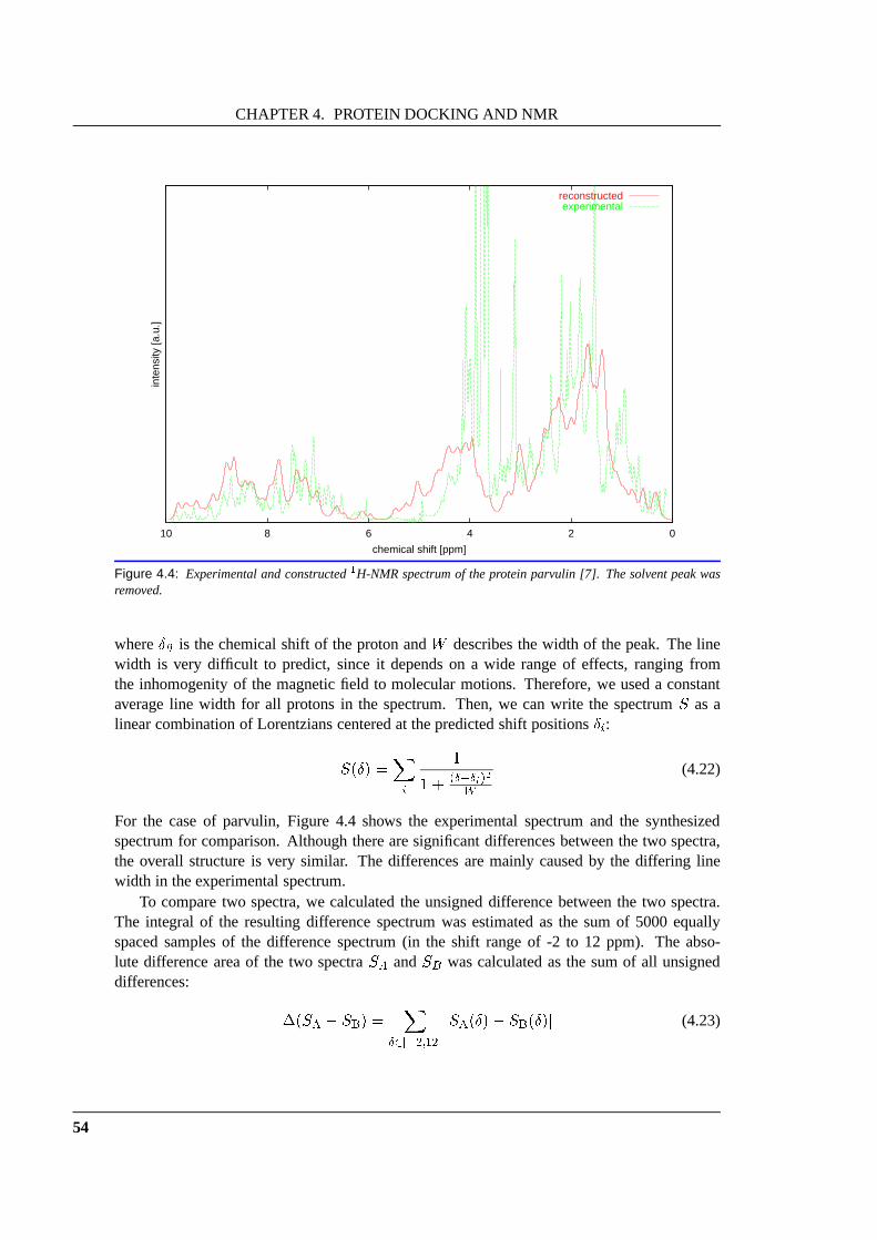
CHAPTER 4. PROTEIN DOCKING AND NMR
0246810
inte
nsity
[a.u
.]
chemical shift [ppm]
reconstructedexperimental
Figure 4.4: Experimental and constructed1H-NMR spectrum of the protein parvulin [7]. The solvent peakwasremoved.
whereÆ0 is the chemical shift of the proton andW describes the width of the peak. The linewidth is very difficult to predict, since it depends on a wide range of effects, ranging fromthe inhomogenity of the magnetic field to molecular motions.Therefore, we used a constantaverage line width for all protons in the spectrum. Then, we can write the spectrumS as alinear combination of Lorentzians centered at the predicted shift positionsÆi:S(Æ) =Xi 11 + (Æ�Æi)2W (4.22)
For the case of parvulin, Figure 4.4 shows the experimental spectrum and the synthesizedspectrum for comparison. Although there are significant differences between the two spectra,the overall structure is very similar. The differences are mainly caused by the differing linewidth in the experimental spectrum.
To compare two spectra, we calculated the unsigned difference between the two spectra.The integral of the resulting difference spectrum was estimated as the sum of 5000 equallyspaced samples of the difference spectrum (in the shift range of -2 to 12 ppm). The abso-lute difference area of the two spectraSA andSB was calculated as the sum of all unsigneddifferences: �(SA � SB) = XÆ2[�2;12℄ jSA(Æ)� SB(Æ)j (4.23)
54

4.3. EXPERIMENTAL RESULTS
The resulting difference area� was used as a measure of similarity between the two spectraand for ranking the docking results.
4.3 Experimental Results
In order to find a suitable test set for our approach we searched the contents of the BMRB(BioMagResBank [108]) for suitable protein complexes of known three-dimensional structureand available1H-NMR spectra. Unfortunately, the number of candidates is very small. Weidentified four candidates where the BMRB contained rather complete shift data of the complexand a corresponding structure was deposited in the Protein Data Bank (PDB, [9]): the complexof calmodulin with the Ca2+-calmodulin-dependent protein kinase kinase [94], the complex ofcalmodulin with a binding peptide of the Ca2+-pump [30], the complex of S100B(��) with apeptide derived from p53 [104], and the two identical subunits of the homodimer S100B(��).
4.3.1 Methods
4.3.1.1 Preparation of Structures and Rigid Body Docking
All complex structures were retrieved from the PDB (PDB IDs 1DT7, 1CFF, and 1CKK). Fromeach structure containing several models, we selected the first model in the file. Missing hydro-gens were added and all hydrogen positions were optimized inthe complex using the AMBER94 force field [22]. The complex structures were then separated into two files each containingone of the complexed proteins or peptides, which were used inour docking algorithm.
For each example, we carried out a rigid-body docking using the algorithm described in [70,71]. The algorithm generates a list of tentative complex structures which are ranked withrespect to geometric and energetic scoring functions.
4.3.1.2 NMR Chemical Shift Calculation
Out shift model decomposes the total chemical shiftÆ of a proton into four componentsÆ = Ælo al + ÆJB + Æaniso + Æes (4.24)
whereÆlo al is the so-called random coil shift,Æaniso is the secondary shift caused by the mag-netic anisotropy of the peptide bond,ÆJB is the ring current effect as calculated by the Johnson-Bovey theory [47], andÆes is the effect of the electric field.
Electric field effect The electrostatic contribution was approximated using eq 4.20 withthe parameters proposed by Williamson and Asakura [129] forboth C-H and N-H bonds. Theelectric field was calculated via Coulomb’s law with atomic charges taken from the AMBER94 force field [22]. In contrast to our model, the WA model usescharges on the N, H, C�,C, and O atoms only. It has been reported in literature (e.g. [93]) that the use of force fieldcharges yields slightly worse results than the use of charges on the backbone when predictingthe spectra of proteins. A likely reason for this result is the fact that the charged side chains areoften immersed in the solvent and the field arising from thesecharges is shielded by the solvent.
55
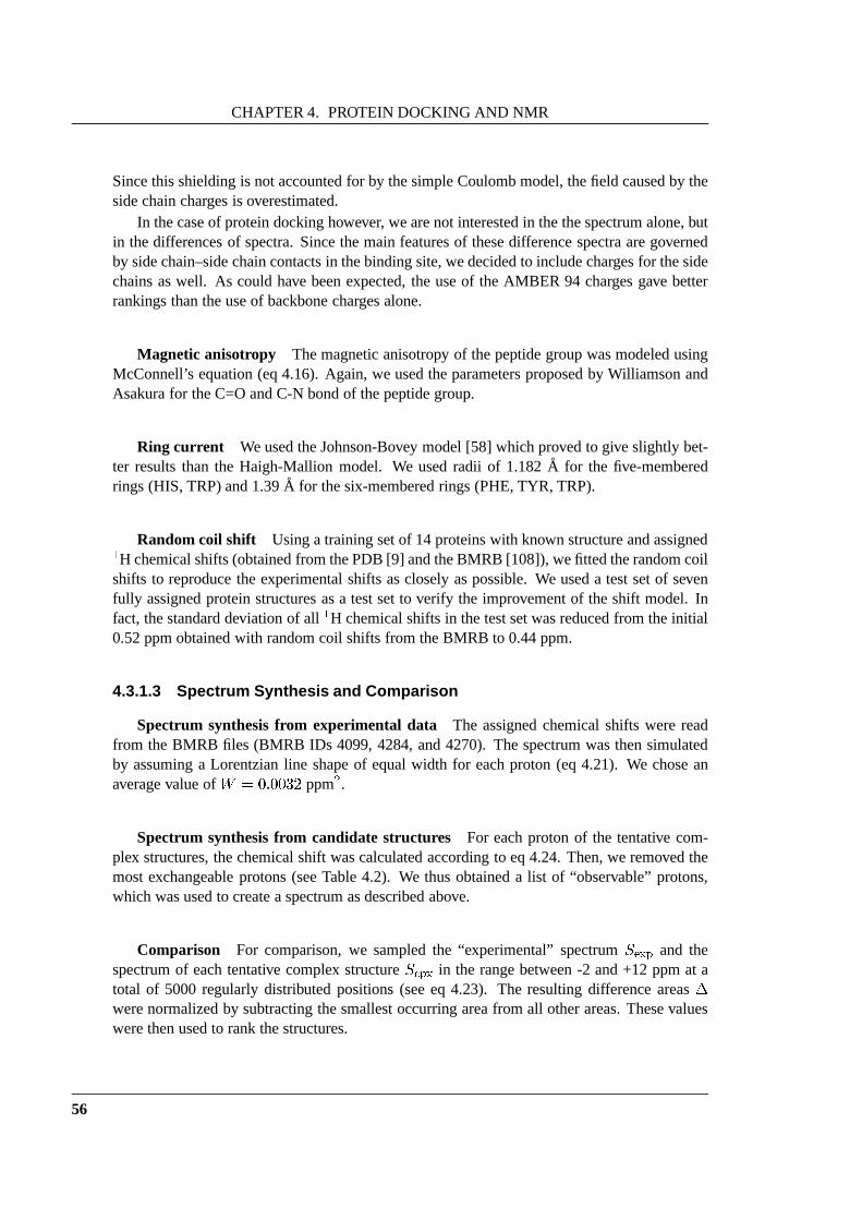
CHAPTER 4. PROTEIN DOCKING AND NMR
Since this shielding is not accounted for by the simple Coulomb model, the field caused by theside chain charges is overestimated.
In the case of protein docking however, we are not interestedin the the spectrum alone, butin the differences of spectra. Since the main features of these difference spectra are governedby side chain–side chain contacts in the binding site, we decided to include charges for the sidechains as well. As could have been expected, the use of the AMBER 94 charges gave betterrankings than the use of backbone charges alone.
Magnetic anisotropy The magnetic anisotropy of the peptide group was modeled usingMcConnell’s equation (eq 4.16). Again, we used the parameters proposed by Williamson andAsakura for the C=O and C-N bond of the peptide group.
Ring current We used the Johnson-Bovey model [58] which proved to give slightly bet-ter results than the Haigh-Mallion model. We used radii of 1.182 A for the five-memberedrings (HIS, TRP) and 1.39A for the six-membered rings (PHE, TYR, TRP).
Random coil shift Using a training set of 14 proteins with known structure and assigned1H chemical shifts (obtained from the PDB [9] and the BMRB [108]), we fitted the random coilshifts to reproduce the experimental shifts as closely as possible. We used a test set of sevenfully assigned protein structures as a test set to verify theimprovement of the shift model. Infact, the standard deviation of all1H chemical shifts in the test set was reduced from the initial0.52 ppm obtained with random coil shifts from the BMRB to 0.44 ppm.
4.3.1.3 Spectrum Synthesis and Comparison
Spectrum synthesis from experimental data The assigned chemical shifts were readfrom the BMRB files (BMRB IDs 4099, 4284, and 4270). The spectrum was then simulatedby assuming a Lorentzian line shape of equal width for each proton (eq 4.21). We chose anaverage value ofW = 0:0032 ppm2.
Spectrum synthesis from candidate structures For each proton of the tentative com-plex structures, the chemical shift was calculated according to eq 4.24. Then, we removed themost exchangeable protons (see Table 4.2). We thus obtaineda list of “observable” protons,which was used to create a spectrum as described above.
Comparison For comparison, we sampled the “experimental” spectrumSexp and thespectrum of each tentative complex structureS px in the range between -2 and +12 ppm at atotal of 5000 regularly distributed positions (see eq 4.23). The resulting difference areas�were normalized by subtracting the smallest occurring areafrom all other areas. These valueswere then used to rank the structures.
56

4.3. EXPERIMENTAL RESULTS
0
5
10
15
20
25
30
35
40
0 200 400 600 800 1000 1200 1400 1600 1800 2000
RM
SD
[A]
difference area [a.u.]
Figure 4.5: Results of the docking of the S100B(��) dimer.
0
5
10
15
20
25
30
35
40
45
50
55
0 200 400 600 800 1000 1200 1400 1600 1800
RM
SD
[A]
difference area [a.u.]
Figure 4.6: Results of the docking of calmodulin with the binding peptide of the Ca2+-pump.
4.3.2 Results
The rigid docking of the four test cases resulted in four setsof tentative complex structures(each set with 24 to 121 different structures). For each of the potential complex structures, we
57

CHAPTER 4. PROTEIN DOCKING AND NMR
0
5
10
15
20
25
30
0 500 1000 1500 2000 2500 3000 3500
RM
SD
[A]
difference area [a.u.]
Figure 4.7: Results of the docking of calmodulin with the Ca2+-calmodulin-dependent protein kinase kinase.
0
10
20
30
40
50
60
0 500 1000 1500 2000 2500 3000
RM
SD
[A]
difference area [a.u.]
Figure 4.8: Results of the docking of the S100B(��) dimer with a peptide derived from p53.
calculated the1H-NMR spectra and determined the difference area between this spectrum andthe experimental complex spectrum. In the case of S100B(��), the BMRB did not containthe complete shift data of the peptide in complex with the S100(��) homodimer, but only theshifts of the homodimer itself.
58

4.3. EXPERIMENTAL RESULTS
0
5
10
15
20
25
30
35
40
45
50
-8 -6 -4 -2 0 2 4 6 8
RM
SD
[A]
ACE [kcal/mol]
Figure 4.9: Results of the conventional docking of the S100B(��) dimer with a peptide derived from p53. NoNMR data was used. Instead, we employed the Atomic Contact Energy (ACE) by Zhang et al. [132] as a scoringfunction.
Initial experiments showed that the ranking of structures was significantly improved, ifthe contributions stemming from the magnetic anisotropy ofthe peptide group were not in-cluded. This result seems surprising at first sight, but a detailed analysis of the shifts lead tothe conclusion, that the effect is caused by structural overlaps. Slightly overlapping structuresare a typical result of rigid-body docking algorithms. Evensmall deviations of the true com-plex structure can bring individual protons into a closer spatial vicinity to anisotropic groupsthan could be expected from the atoms’ van-der-Waals radii.Since the effect of the magneticanisotropy grows with the third power of the inverse distance, these collisions lead to enormouschanges in the chemical shift. Furthermore, the effect of the magnetic anisotropy is basicallya local effect; it depends strongly on the backbone torsion angles (i.e. the secondary structure)and has a much more limited range than ring current and electric field effects. Therefore, themagnetic anisotropy of the backbone of one of the proteins should not influence the shifts ofits docking partner significantly. Hence, we excluded the effect of the magnetic anisotropybetween the two docking partners, but included it within each of the partners.
The results of the docking experiments are shown in Figs. 4.5, 4.6, 4.7, and 4.8. In thesefigures, every point represents a single tentative complex structure. It shows the root meansquare deviation (RMSD, y-axis) of the structure from the true complex structure and the nor-malized difference area of the candidate’s spectrum (x-axis). Good approximations of the truecomplex structure should thus be expected in the lower left corner of the graph.
Except for the complex of calmodulin with the binding peptide of the Ca2+-pump, scoringaccording to the difference area always identified a good approximation of the true complexstructure. The separation between true and false positiveswas good for the S100B(��) dimer
59

CHAPTER 4. PROTEIN DOCKING AND NMR
and for the complex of calmodulin and kinase, and excellent for the complex of S100B(��)and the p53-peptide.
The latter fact is very surprising, since the docking of the small p53-derived peptide (22amino acids) was impossible using conventional methods. Wetested different energy-basedscoring functions but we were not able to obtain a correct ranking. Fig. 4.9 shows the result ofthe docking using the Atomic Contact Energy (ACE) developedby Zhanget al.[132]. The firstapproximation of the true complex structure is ranked as number 48. Other scoring functions,e.g. the use of geometric methods [60] or the inclusion of electrostatics, gave very similarresults. The problems with this docking example stem basically from the small binding site ofthe peptide. Most docking algorithms favor structures where the peptide has a larger contactarea with the protein. In this case, the use of NMR data was theonly possibility to correctlypredict the complex structure.
For the complex of calmodulin with the binding peptide of theCa2+-pump, a false positivestructure was ranked number one, followed by the major part of the true positive structures.The reasons for this failure are not yet clear.
60
Chapter 5
Discussion
Semi-flexible docking
We proposed two new approaches for semi-flexible protein docking. In a first step, a rigid-bodydocking algorithm generates a set of tentative complex structures. In a second step, a side chaindemangling step, we resolve problems arising from side chain overlaps in the binding site. Thisdemangling results in physically meaningful complex conformations that can be ranked withstandard energetic functions.
The side chain demangling is based upon a reduction of the side chain placement problem toa combinatorial optimization problem by discretizing the side chain conformations to rotamers.The first approach is based on a simple greedy heuristic. It searches for minimal solutions inthe enumeration tree spanned by the rotamers of all side chains in the binding site and avoidscombinatorial explosion by limiting the number of leaves ineach tree layer. This approachis very fast, although it usually yields suboptimal solutions. The quality of these solutions isnevertheless sufficient to solve the side chain placement problem in protein docking.
The second approach is a branch-&-cut technique that is based on an ILP formulation of theside chain placement problem. After identifying several classes of facet-defining inequalitiesfor the side chain placement polytope and devising a separation algorithms for a subclass ofthese inequalities, we were able to solve the side chain placement problem to optimality.
Both approaches correctly predict the structure of three difficult test cases for protein dock-ing that cannot be solved using rigid-body docking approaches. Running times are moderateand mainly governed by the energetic evaluation of the final structures and not by the side chainplacement step.
There is still room for significant improvements of the method. The fact that we can solvethe problem optimally unfortunately does not imply that we can solve thebiological problemoptimally. Instead, we solve an abstract representation ofproblem. There are two main differ-ences between the two problems. First, we find an optimal solution with respect to an energeticfunction (the force field). This function is only a coarse approximation of the true energiesoccurring in the protein. Second, the restriction of the side chain conformational space to therotamer conformations possibly exclude some rare conformations that may occur in nature.Both points leave much room for improvements. For example, the AMBER force field doesnot account for solvation effects. In contrast, the recently developed CHARMM EEF1 forcefield [66] introduces an additional force field term for the solvation energy. Since the solvationenergy is expressed as a pairwise interaction, our energetic decomposition still holds for thisforce field and it might significantly improve the results. The rotamer library we used couldalso be replaced by a more detailed library, thus representing also less frequently occurringconformations.
Besides these improvements of the fundamental model, algorithmic and implementationimprovements are possible as well. An interesting approachmay be the use of branch-&-

CHAPTER 5. DISCUSSION
price techniques. Also the most time-consuming step for theside chain placement problem(the calculation of the interaction energies) could be spedup by integrating the calculationinto the greedy algorithm and thus calculating only those energies that are required, instead ofprecomputing all interactions in an initial step.
The key component of the algorithm, the side chain placementalgorithm, can be applied torelated problems like protein structure prediction or ligand docking as well.
NMR-based docking
We also presented a new approach to protein docking that directly incorporates experimentalstructural data of the protein complex into the docking algorithm. It is the first algorithm thatpermits the use of NMR spectra for the validation and rankingof docking results. NMR-derived distance constraints have been widely used in ligand docking to improve the results,but these constraints have to be determined manually from fully assigned NMR spectra. Ourmethod avoids this difficult and time-consuming manual preprocessing of the experimentaldata. Instead, we use the structures proposed by the dockingalgorithm to simulate the NMRspectrum of the complex and compare this spectrum directly to the experimental spectrum.
We implemented and tested several empirical models for NMR shift prediction. The modelwe used in our final experiments was based on existing models,that were combined and repa-rameterized. We also had to adapt the contributions arisingfrom the magnetic anisotropy of thepeptide bond and the electric field effect to the special requirements of the docking problem.The scoring function used for the docking is based on the difference area between the predictedand the experimental spectrum.
We chose a test set of four protein complexes: the complex of calmodulin with the Ca2+-calmodulin-dependent protein kinase kinase, the complex of calmodulin with a binding peptideof the Ca2+-pump, the complex of S100B(��) with a peptide derived from p53, and the twoidentical subunits of the homodimer S100B(��). For three of these complexes, our algorithmcould clearly identify the true complex structure. in the case of the fourth complex (calmodulinwith the binding peptide of the Ca2+-pump) one false positive structure was ranked slightlybetter than the first true positive structure. The usefulness of the method has been provenfor the complex of S100B(��) and the p53-peptide. We tried to predict the structure of thecomplex using several energy-based scoring functions, butwere unable to predict the correctstructure. When using our NMR-based scoring function, we obtained an excellent separationof true positives and false positives: there was no false positive among the first 20 candidates.Obviously, the method is a useful tool even in those cases, where energy-based methods fail.
One major problem when testing the algorithm was clearly theamount of data available.Since experimental spectra are not available from public data banks, we were forced to recon-struct the spectra from the deposited shift assignments andeven then, there were only four testcases available. The main reason for the scarcity of data is the fact that X-ray crystallographyis still the more common method for structure elucidation ofprotein-protein complexes. So theapproach has still to be validated with direct data, which wehope to obtain from a collaborationwith NMR spectroscopists.
We are also positive that the shift model proposed here can still be significantly improved.We carried out a series of quantum mechanical calculations to verify and reparameterize some
62

of the shift contributions. In the course of these experiments, we found that most models arequite coarse approximations. This observation is in accordance with recent developments inthe field of NMR shift modeling, since many researchers in this field are currently working onquantum mechanical calculation of so-called shielding hypersurfaces. The current model alsoconsiders only a subset of all known effects. A detailed analysis of those shifts that showed thelargest deviations between predicted and experimental shift values lead to the conclusion thathydrogen bonds and solvent effects play an important role. Models for both effects still haveto be developed.
Further improvements should also address the prediction ofthe peak widths. The line widthis caused (at least in parts) by the molecular motion of the protein. Therefore, it seems plausibleto obtain better results by calculating the spectra as a timeaverage over trajectories obtainedfrom Molecular Dynamics Simulations. An interesting question is also whether this approachcan be extended to ligand docking as well or whether the changes in the spectrum caused bysmall ligands are too insignificant in comparison with the protein spectrum.
Finally, and perhaps the most interesting application, is the use of the new scoring functionin protein structure prediction. In protein structure prediction, the three-dimensional struc-ture of a protein is predicted from its sequence alone. Similar to docking algorithms, proteinstructure prediction methods generate a set of potential structures, which are then ranked withrespect to some energy function. The fact that the spectra-based scoring function gave verypromising results for protein docking raises hopes that similar results can be obtained for pro-tein structure prediction as well. These hopes are based on the fact that structural differencesbetween the candidates obtained from structure predictionalgorithms are larger than the differ-ences between the candidates generated for protein docking. The combination of protein struc-ture prediction and NMR spectra prediction could then speedup the process of structure eluci-dation for proteins significantly by generating good initial structure models and initial guessesfor the shift assignment. Eventually, such methods could pave the way to high-throughputmethods for protein structure elucidation, one of the foremost goals of proteomics.
63


Part III
BALL

66

Chapter 6
Design and Implementation
6.1 Introduction
Implementation is often the biggest hurdle when testing newideas and approaches. This isespecially true for the field of Molecular Modeling, where the implementation of standardtechniques (e.g.Molecular Mechanics) often requires several man years of hard work to imple-ment. Obviously, this problem can be tackled using softwarethat was specially designed forRapid Application Development(RAD, also calledRapid Software Prototyping).
The need for appropriate RAD tools becomes even more obviouswhen looking at the soft-ware that is currently used. The majority of software packages currently in use in MolecularModeling is not only written in FORTRAN, but often lacks a thorough documentation as well.The language FORTRAN itself is not very suitable for Rapid Software Prototyping, as the pro-cedural programming paradigm is clearly inferior to the Object-Oriented approach with respectto reusability. Nevertheless, FORTRAN packages are still immensely successful, because peo-ple got used to their, often awkward, interfaces and people prefer the time a reimplementationwould require preferably for other tasks.
We already discussed a number of software packages that are frequently used for MolecularModeling in the introduction (Part I). To summarize this discussion, one can say that thesepackages provide the required functionality, but they are hardly reusable and (apart from someexceptions) not object-oriented. There is no software available that is specifically designed forRapid Application Development. For this reason, we designed and implemented BALL – theBiochemical Algorithms Library.
When we started the BALL project (under the tentative project title BioLEDA at that time),we did not spend much time on design. In fact, we started in June 1996 with just one page de-scribing the attributes of nine classes (System , Molecule , Fragment , Atom, Sequence ,BioMolecule , RNA, DNA, andProtein ). Based on this kernel of primitive classes, wewanted to implement algorithms for protein-protein docking.
A vast amount of code was implemented at the beginning of the project. It was not until wefirst wanted to use the code in real applications, that we realized it was completely unusable,although it fulfilled all our “specifications”. Thus, we learned the need for a thorough designthe hard way. The current version of BALL was designed more carefully and we also made useof some more advanced software engineering techniques.
BALL was first designed to be aclass library, but it soon turned out that instead we neededaframework. Contrary to a typical class library, the classes of a framework also provide abstractor empty methods. The framework defines the cooperation of its classes and the developerusually just fills in the required functionality by defining new subclasses. These subclassesredefine the abstract or empty methods of their respective base classes. Due to inheritance, thecooperation of the subclasses is still defined by the framework.
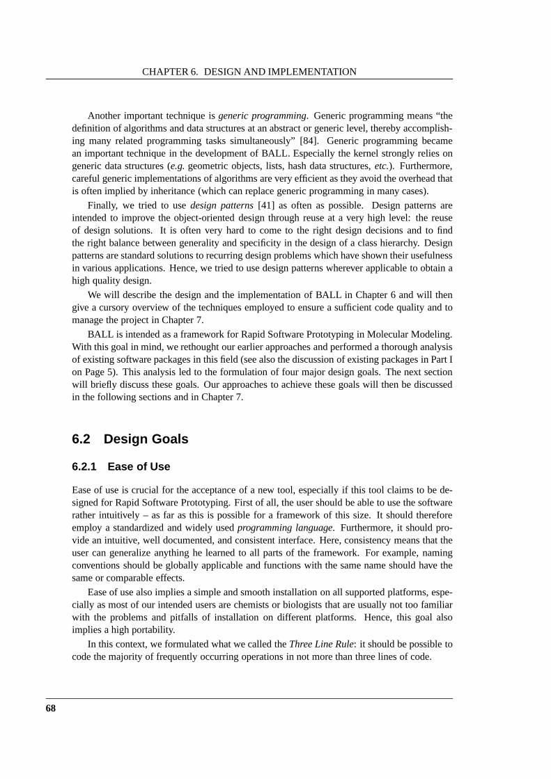
CHAPTER 6. DESIGN AND IMPLEMENTATION
Another important technique isgeneric programming. Generic programming means “thedefinition of algorithms and data structures at an abstract or generic level, thereby accomplish-ing many related programming tasks simultaneously” [84]. Generic programming becamean important technique in the development of BALL. Especially the kernel strongly relies ongeneric data structures (e.g.geometric objects, lists, hash data structures,etc.). Furthermore,careful generic implementations of algorithms are very efficient as they avoid the overhead thatis often implied by inheritance (which can replace generic programming in many cases).
Finally, we tried to usedesign patterns[41] as often as possible. Design patterns areintended to improve the object-oriented design through reuse at a very high level: the reuseof design solutions. It is often very hard to come to the rightdesign decisions and to findthe right balance between generality and specificity in the design of a class hierarchy. Designpatterns are standard solutions to recurring design problems which have shown their usefulnessin various applications. Hence, we tried to use design patterns wherever applicable to obtain ahigh quality design.
We will describe the design and the implementation of BALL inChapter 6 and will thengive a cursory overview of the techniques employed to ensurea sufficient code quality and tomanage the project in Chapter 7.
BALL is intended as a framework for Rapid Software Prototyping in Molecular Modeling.With this goal in mind, we rethought our earlier approaches and performed a thorough analysisof existing software packages in this field (see also the discussion of existing packages in Part Ion Page 5). This analysis led to the formulation of four majordesign goals. The next sectionwill briefly discuss these goals. Our approaches to achieve these goals will then be discussedin the following sections and in Chapter 7.
6.2 Design Goals
6.2.1 Ease of Use
Ease of use is crucial for the acceptance of a new tool, especially if this tool claims to be de-signed for Rapid Software Prototyping. First of all, the user should be able to use the softwarerather intuitively – as far as this is possible for a framework of this size. It should thereforeemploy a standardized and widely usedprogramming language. Furthermore, it should pro-vide an intuitive, well documented, and consistent interface. Here, consistency means that theuser can generalize anything he learned to all parts of the framework. For example, namingconventions should be globally applicable and functions with the same name should have thesame or comparable effects.
Ease of use also implies a simple and smooth installation on all supported platforms, espe-cially as most of our intended users are chemists or biologists that are usually not too familiarwith the problems and pitfalls of installation on differentplatforms. Hence, this goal alsoimplies a high portability.
In this context, we formulated what we called theThree Line Rule: it should be possible tocode the majority of frequently occurring operations in notmore than three lines of code.
68

6.2. DESIGN GOALS
6.2.2 Functionality
Functionality is of obvious importance. We can only expect wide acceptance of our software,if it is able to save the potential user a major amount of time.Thus, it should provide most ofthe standard functionality and leave only the implementation of specialized or new techniquesto the user. And even there the user should be able to take advantage of existing data structuresto speed up the development.
This is a very ambitious aim, because Molecular Modeling andComputational MolecularBiology are rather large and diverse fields and it seems impossible to provide all function-ality anybody might require. So we had to put a focus on the more elementary things thatare required by the majority of applications and we restricted the functionality to the field ofMolecular Modeling and especially protein docking.
We identified four key areas of functionality that are used inmost applications. First ofall, we need somemolecular data structuresto represent molecules, atoms and the like. Thesedata structures typically hold structural or experimentaldata that is read from disk, so weneed support forimport and export in various file formats. In many applications, this data isthen manipulated usingMolecular Mechanicsmethods. These are empirical models describingproperties and dynamic behavior of matter at the atomic level. Finally, thevisualizationof theresulting structures is usually desirable.
6.2.3 Openness
Since we cannot provide all functionality and we also do not want to reimplement existingalgorithms, it was also an important aim to provide a sufficient openness, meaning compatibil-ity with other class libraries. For example, from the very start we planned the integration ofLEDA [78], ABACUS [59], and CGAL [31].
Furthermore, openness includesextensibilityandmodularity, i.e. it should be simple to addnew functionality and data structures without changing theexisting code.
6.2.4 Robustness
The term robustness describes the code’s ability to cope with unexpected or faulty data. A goodexample of such faulty data is the PDB file format [9] for crystallographic structures. Thisformat is the most common format for structural data and is well standardized. Nevertheless,only very few files circulating among scientists adhere to this standard for historical as wellas for practical reasons. Strange as it may seem, but the implementation of a robust code forreading these files is a very demanding task. Implementing a file reader accepting standardcompliant files is simple enough, but is not sufficient as onlyvery few files could be read.Reliable reading of non-compliant files requires quite somebiochemical knowledge and non-trivial heuristics to extract as much of the data as possible.
According to the 80-20 rule [81], which states that a typicalprogram spends 80 percentof its time executing 20 percent of the code, we decided to optimize only the computationallydemanding code sections and sacrifice a bit of performance toan overall robust and reliablecode. Since robustness also implies correctness, we also require techniques for software testing.
69
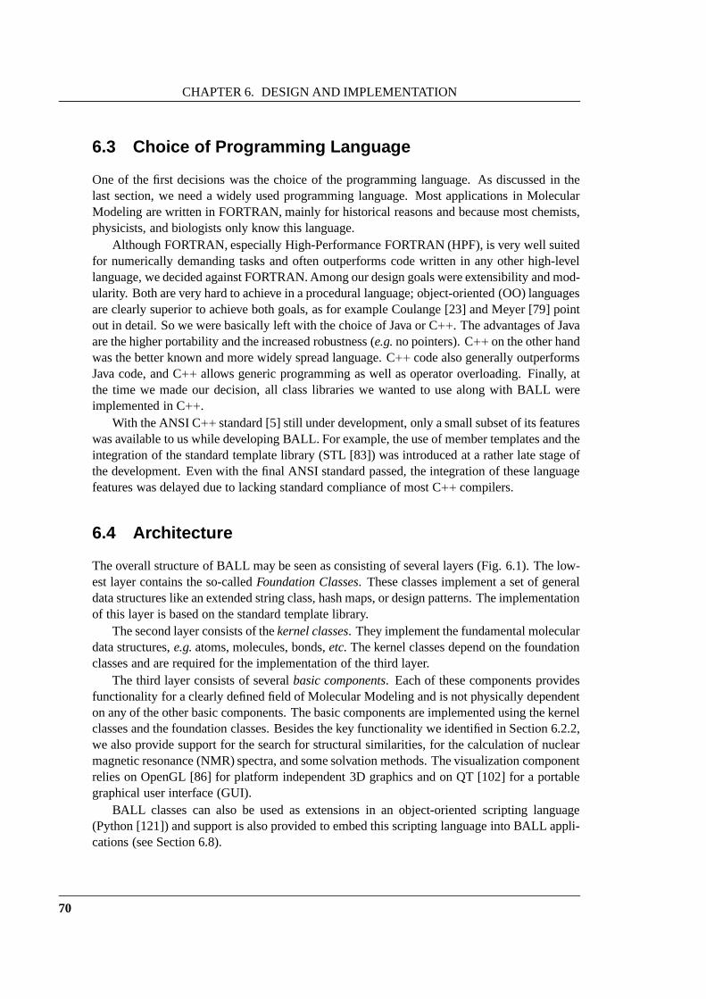
CHAPTER 6. DESIGN AND IMPLEMENTATION
6.3 Choice of Programming Language
One of the first decisions was the choice of the programming language. As discussed in thelast section, we need a widely used programming language. Most applications in MolecularModeling are written in FORTRAN, mainly for historical reasons and because most chemists,physicists, and biologists only know this language.
Although FORTRAN, especially High-Performance FORTRAN (HPF), is very well suitedfor numerically demanding tasks and often outperforms codewritten in any other high-levellanguage, we decided against FORTRAN. Among our design goals were extensibility and mod-ularity. Both are very hard to achieve in a procedural language; object-oriented (OO) languagesare clearly superior to achieve both goals, as for example Coulange [23] and Meyer [79] pointout in detail. So we were basically left with the choice of Java or C++. The advantages of Javaare the higher portability and the increased robustness (e.g.no pointers). C++ on the other handwas the better known and more widely spread language. C++ code also generally outperformsJava code, and C++ allows generic programming as well as operator overloading. Finally, atthe time we made our decision, all class libraries we wanted to use along with BALL wereimplemented in C++.
With the ANSI C++ standard [5] still under development, only a small subset ofits featureswas available to us while developing BALL. For example, the use of member templates and theintegration of the standard template library (STL [83]) wasintroduced at a rather late stage ofthe development. Even with the final ANSI standard passed, the integration of these languagefeatures was delayed due to lacking standard compliance of most C++ compilers.
6.4 Architecture
The overall structure of BALL may be seen as consisting of several layers (Fig. 6.1). The low-est layer contains the so-calledFoundation Classes. These classes implement a set of generaldata structures like an extended string class, hash maps, ordesign patterns. The implementationof this layer is based on the standard template library.
The second layer consists of thekernel classes. They implement the fundamental moleculardata structures,e.g.atoms, molecules, bonds,etc.The kernel classes depend on the foundationclasses and are required for the implementation of the thirdlayer.
The third layer consists of severalbasic components. Each of these components providesfunctionality for a clearly defined field of Molecular Modeling and is not physically dependenton any of the other basic components. The basic components are implemented using the kernelclasses and the foundation classes. Besides the key functionality we identified in Section 6.2.2,we also provide support for the search for structural similarities, for the calculation of nuclearmagnetic resonance (NMR) spectra, and some solvation methods. The visualization componentrelies on OpenGL [86] for platform independent 3D graphics and on QT [102] for a portablegraphical user interface (GUI).
BALL classes can also be used as extensions in an object-oriented scripting language(Python [121]) and support is also provided to embed this scripting language into BALL appli-cations (see Section 6.8).
70

6.5. THE FOUNDATION CLASSES
Solvation StructureMolecular NMRMechanics PythonExtensions
Export
InterpreterFileImport/Visualization
BallVIEW
Embedded
QT
OpenGL STL
KERNEL
Foundation Classes
Application
OO Scripting Language (Python)
Figure 6.1: Overview of the structure of BALL. The basic components are in white, the scripting language supportin yellow and external libraries that are not part of BALL arein gray.
The architecture and the high-level design of the three layers will be described in moredetail in the next three sections. Due to the large number of classes in BALL, we had to restrictthis overview to some of the more interesting examples.
6.5 The Foundation Classes
This section describes a selection of the most important foundation classes as well as somecommon definitions and functions required for the implementation of the kernel and the foun-dation classes.
6.5.1 Global Definitions
BALL defines a number of global type definitions and constant definitions. The types that areused in BALL are declared inCOMMON/global.h . These definitions are typedefs to primi-tive types as determined by configure. For example, BALL usesthe typePointerSizeIntto describe an integer type with the same bit width as the pointers on the respective platform.configure determines the correct type for this definition and includesit into config.hwhich is included byCOMMON/global.h . By defining these types we achieve a better porta-bility. Especially the compatibility between 32 bit systems and 64 bit systems relies heavilyupon the use of these types (see also the implementation of object persistence in Section 6.5.3).
The namespaceConstants holds a large number of constant definitions. These aremainly physical and chemical constants (e.g.speed of light, electron mass, etc.) and math-ematical constants (e.g.�, e). The BALL kernel uses only these constants, thus reducing thepossibility of errors due to wrong constants. This also reduces numerical inconsistencies be-tween different code parts.
71
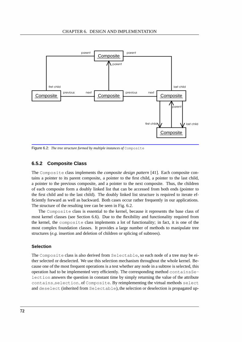
CHAPTER 6. DESIGN AND IMPLEMENTATION
Composite
Composite CompositeComposite
Composite
first child last child
previous next previous next
parent
parent
parent
parent
first child last child
Figure 6.2: The tree structure formed by multiple instances ofComposite
6.5.2 Composite Class
TheComposite class implements thecomposite design pattern[41]. Each composite con-tains a pointer to its parent composite, a pointer to the firstchild, a pointer to the last child,a pointer to the previous composite, and a pointer to the nextcomposite. Thus, the childrenof each composite form a doubly linked list that can be accessed from both ends (pointer tothe first child and to the last child). The doubly linked list structure is required to iterate ef-ficiently forward as well as backward. Both cases occur rather frequently in our applications.The structure of the resulting tree can be seen in Fig. 6.2.
The Composite class is essential to the kernel, because it represents the base class ofmost kernel classes (see Section 6.6). Due to the flexibilityand functionality required fromthe kernel, thecomposite class implements a lot of functionality; in fact, it is one ofthemost complex foundation classes. It provides a large numberof methods to manipulate treestructures (e.g.insertion and deletion of children or splicing of subtrees).
Selection
TheComposite class is also derived fromSelectable , so each node of a tree may be ei-ther selected or deselected. We use this selection mechanism throughout the whole kernel. Be-cause one of the most frequent operations is a test whether any node in a subtree is selected, thisoperation had to be implemented very efficiently. The corresponding methodcontainsSe-lection answers the question in constant time by simply returning the value of the attributecontains selection of Composite . By reimplementing the virtual methodsselectanddeselect (inherited fromSelectable ), the selection or deselection is propagated up-
72
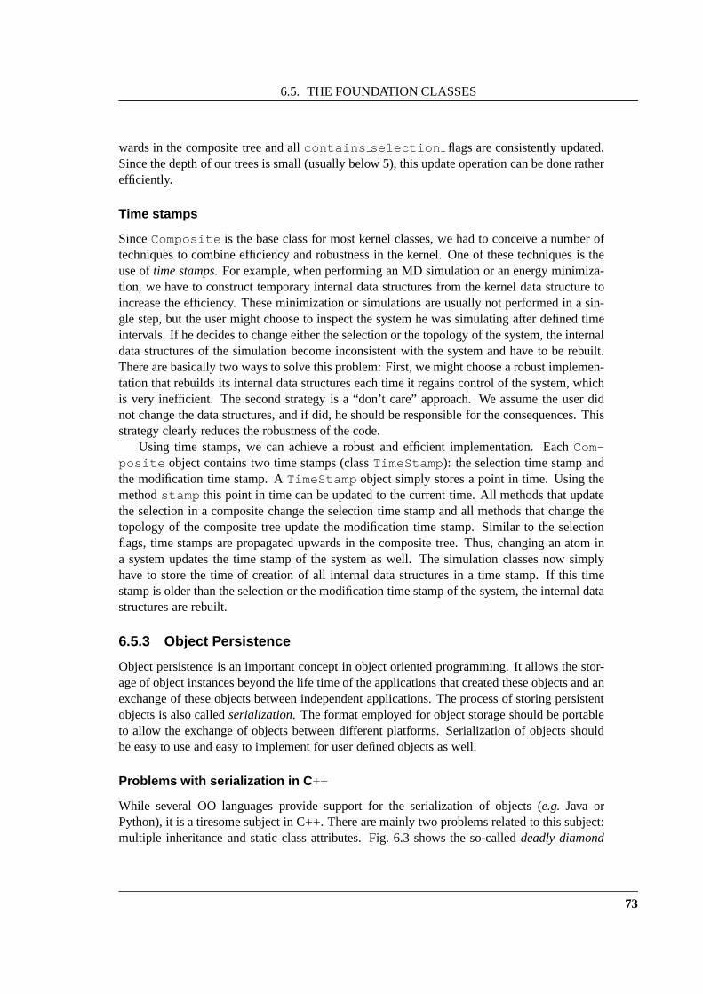
6.5. THE FOUNDATION CLASSES
wards in the composite tree and allcontains selection flags are consistently updated.Since the depth of our trees is small (usually below 5), this update operation can be done ratherefficiently.
Time stamps
SinceComposite is the base class for most kernel classes, we had to conceive anumber oftechniques to combine efficiency and robustness in the kernel. One of these techniques is theuse oftime stamps. For example, when performing an MD simulation or an energy minimiza-tion, we have to construct temporary internal data structures from the kernel data structure toincrease the efficiency. These minimization or simulationsare usually not performed in a sin-gle step, but the user might choose to inspect the system he was simulating after defined timeintervals. If he decides to change either the selection or the topology of the system, the internaldata structures of the simulation become inconsistent withthe system and have to be rebuilt.There are basically two ways to solve this problem: First, wemight choose a robust implemen-tation that rebuilds its internal data structures each timeit regains control of the system, whichis very inefficient. The second strategy is a “don’t care” approach. We assume the user didnot change the data structures, and if did, he should be responsible for the consequences. Thisstrategy clearly reduces the robustness of the code.
Using time stamps, we can achieve a robust and efficient implementation. EachCom-posite object contains two time stamps (classTimeStamp ): the selection time stamp andthe modification time stamp. ATimeStamp object simply stores a point in time. Using themethodstamp this point in time can be updated to the current time. All methods that updatethe selection in a composite change the selection time stampand all methods that change thetopology of the composite tree update the modification time stamp. Similar to the selectionflags, time stamps are propagated upwards in the composite tree. Thus, changing an atom ina system updates the time stamp of the system as well. The simulation classes now simplyhave to store the time of creation of all internal data structures in a time stamp. If this timestamp is older than the selection or the modification time stamp of the system, the internal datastructures are rebuilt.
6.5.3 Object Persistence
Object persistence is an important concept in object oriented programming. It allows the stor-age of object instances beyond the life time of the applications that created these objects and anexchange of these objects between independent applications. The process of storing persistentobjects is also calledserialization. The format employed for object storage should be portableto allow the exchange of objects between different platforms. Serialization of objects shouldbe easy to use and easy to implement for user defined objects aswell.
Problems with serialization in C ++
While several OO languages provide support for the serialization of objects (e.g. Java orPython), it is a tiresome subject in C++. There are mainly two problems related to this subject:multiple inheritance and static class attributes. Fig. 6.3shows the so-calleddeadly diamond
73
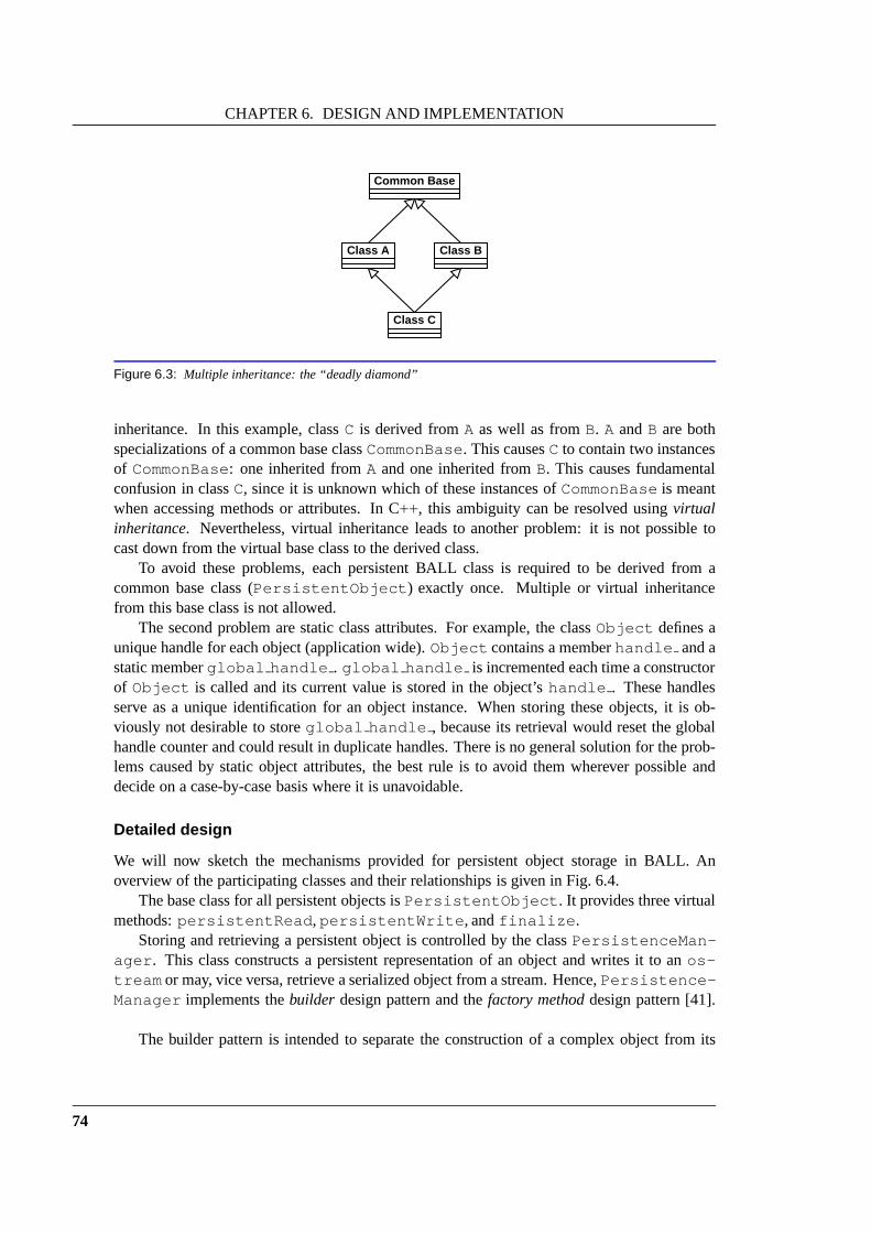
CHAPTER 6. DESIGN AND IMPLEMENTATION
Common Base
Class C
Class A Class B
Figure 6.3: Multiple inheritance: the “deadly diamond”
inheritance. In this example, classC is derived fromA as well as fromB. A andB are bothspecializations of a common base classCommonBase. This causesC to contain two instancesof CommonBase: one inherited fromA and one inherited fromB. This causes fundamentalconfusion in classC, since it is unknown which of these instances ofCommonBaseis meantwhen accessing methods or attributes. In C++, this ambiguity can be resolved usingvirtualinheritance. Nevertheless, virtual inheritance leads to another problem: it is not possible tocast down from the virtual base class to the derived class.
To avoid these problems, each persistent BALL class is required to be derived from acommon base class (PersistentObject ) exactly once. Multiple or virtual inheritancefrom this base class is not allowed.
The second problem are static class attributes. For example, the classObject defines aunique handle for each object (application wide).Object contains a memberhandle and astatic memberglobal handle . global handle is incremented each time a constructorof Object is called and its current value is stored in the object’shandle . These handlesserve as a unique identification for an object instance. Whenstoring these objects, it is ob-viously not desirable to storeglobal handle , because its retrieval would reset the globalhandle counter and could result in duplicate handles. Thereis no general solution for the prob-lems caused by static object attributes, the best rule is to avoid them wherever possible anddecide on a case-by-case basis where it is unavoidable.
Detailed design
We will now sketch the mechanisms provided for persistent object storage in BALL. Anoverview of the participating classes and their relationships is given in Fig. 6.4.
The base class for all persistent objects isPersistentObject . It provides three virtualmethods:persistentRead , persistentWrite , andfinalize .
Storing and retrieving a persistent object is controlled bythe classPersistenceMan-ager . This class constructs a persistent representation of an object and writes it to anos-tream or may, vice versa, retrieve a serialized object from a stream. Hence,Persistence-Manager implements thebuilder design pattern and thefactory methoddesign pattern [41].
The builder pattern is intended to separate the construction of a complex object from its
74
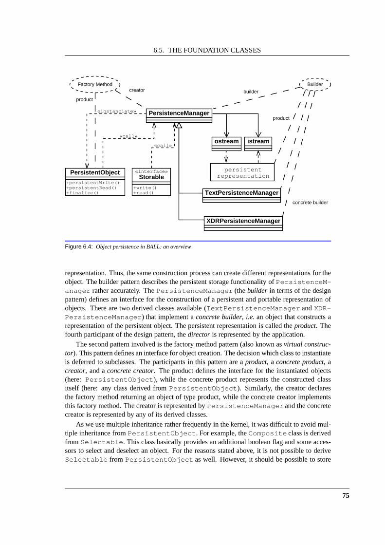
6.5. THE FOUNDATION CLASSES
PersistentObject
+persistentWrite()+persistentRead()+finalize()
PersistenceManager
istreamostream
«interface»Storable
+write()+read()
«instanciate»
«call»
«call»
BuilderFactory Methodcreator
product
XDRPersistenceManager
TextPersistenceManager
concrete builder
builder
persistentrepresentation
product
Figure 6.4: Object persistence in BALL: an overview
representation. Thus, the same construction process can create different representations for theobject. The builder pattern describes the persistent storage functionality ofPersistenceM-anager rather accurately. ThePersistenceManager (thebuilder in terms of the designpattern) defines an interface for the construction of a persistent and portable representation ofobjects. There are two derived classes available (TextPersistenceManager andXDR-PersistenceManager ) that implement aconcrete builder, i.e. an object that constructs arepresentation of the persistent object. The persistent representation is called theproduct. Thefourth participant of the design pattern, thedirector is represented by the application.
The second pattern involved is the factory method pattern (also known asvirtual construc-tor). This pattern defines an interface for object creation. Thedecision which class to instantiateis deferred to subclasses. The participants in this patternare aproduct, a concrete product, acreator, and aconcrete creator. The product defines the interface for the instantiated objects(here: PersistentObject ), while the concrete product represents the constructed classitself (here: any class derived fromPersistentObject ). Similarly, the creator declaresthe factory method returning an object of type product, while the concrete creator implementsthis factory method. The creator is represented byPersistenceManager and the concretecreator is represented by any of its derived classes.
As we use multiple inheritance rather frequently in the kernel, it was difficult to avoid mul-tiple inheritance fromPersistentObject . For example, theComposite class is derivedfrom Selectable . This class basically provides an additional boolean flag and some acces-sors to select and deselect an object. For the reasons statedabove, it is not possible to deriveSelectable from PersistentObject as well. However, it should be possible to store
75

CHAPTER 6. DESIGN AND IMPLEMENTATION
Atom
+persistentWrite()+persistentRead()
Composite
+persistentWrite()+persistentRead()
PersistentObject
+persistentWrite()+persistentRead()
«interface»Storable
+write()+read()
PropertyManager
+write()+read()
Selectable
+write()+read()
Figure 6.5: TheAtom class and its base classes.
the contents of an instance ofSelectable in a convenient way. This can be achieved bydefining an interface that contains the two methodsread andwrite . These two methods canbe used in the implementation ofpersistentRead andpersistentWrite for storingand retrieving the contents of the base class. Furthermore,it is possible to derive from severalStorable classes without running into problems due to multiple inheritance. The cooper-ation betweenPersistentObject and theStorable interface is illustrated in the classgraph of theAtom class (Fig. 6.5).
Implementation
TextPersistenceManager provides three different layers of methods. Layer 0 providesfundamental methods to store and retrieve primitive data types (e.g.int, float, pointer, string).For each primitive type, there is aput method and aget method. The layer 0 methods im-plement the format of the persistent representation that isproduced. They are implemented bysubclasses ofPersistenceManager . These methods determine the format of the persistentrepresentation (e.g.text or binary).
The layer 1 commands are needed to implement thepersistentWrite andpersis-tentRead methods. They are implemented inPersistenceManager using the layer 0commands. Knowledge of these methods is only required to implement new persistent classes.
To store and retrieve existing objects, the user has to know the level 2 commands alone.They provide methods to assign the input and output streams of the persistence manager and tostore and retrieve objects.
76

6.5. THE FOUNDATION CLASSES
Portability
BALL has been ported to a variety of different platforms. Themain differences between theseplatforms are� word width (32 bit vs. 64 bit machines)� byte order (big endian vs. little endian)� floating point formats
A portable implementation of object persistence has to find platform independent represen-tations for all data types to overcome these differences. First, all pointers are representedinternally (in thePersistenceManager class) using 64 bit types and are also stored thisway. Byte order and floating point formats affect the portable storage of primitive data types.Therefore, the implementation of the layer 0 commands in anyconcrete persistence managerhas to ensure portability. One way to achieve this is the use of text-based formats. This ap-proach is implemented inTextPersistenceManager . This class stores an object in ahuman readable text format. It uses ASCII representations of numbers to achieve portability.However, the resulting representation is large and slow to parse. This class is mainly intendedfor debugging.
The classXDRPersistenceManager produces a much more compact binary format. Itis based upon theXDRformat (External Data Representation). XDR is a standard for portabledata exchange, introduced by SUN Microsystems [115, 111]. It is available on all platformsand was introduced to allow data exchange via the network. For example, remote procedurecalls (RPC) use XDR as their data exchange format. XDR provides methods for packing prim-itive data types (e.g. int, float, string) into four byte packets. These packets arethen writtento a stream. The resulting representation is not human readable, but has little overhead andcan be processed rapidly.XDRPersistenceManager translates the layer 0 commands ofTextPersistenceManager to the corresponding XDR function calls and converts theXDR buffers to a C++ stream and back.
User interface
Using persistence in BALL is rather simple. It requires the instantiation of a persistencemanager, assignment of an input or output stream, and finallythe persistent reading or writingof the object.
1 Protein p = ....; // the object to serialize2 ofstream outstream("test.pers", ios::out); // open outpu t stream3 TextPersistenceManager pm(outstream); // create persist ence manager4 pm << p; // serialization5 outstream.close(); // close the output stream. Done.
Deserializing a persistent object is equally simple:
1 ifstream instream("test.pers"); // open input stream2 TextPersistenceManager pm(instream); // create persiste nce manager3 PersistentObject* po; // define a pointer to a PO
77

CHAPTER 6. DESIGN AND IMPLEMENTATION
4 pm >> po; // deserialization5 instream.close(); // close the input stream67 if (po != 0) // identify the object8 {9 cout << "Read object of type " << typeid(*po).name() << endl;
10 }
Instead of using file streams (as in the two examples above), it is possible to use any fullytransparent stream derived fromistream or ostream . For example, BALL uses theSock-etStream class to exchange persistent objects between different applications using TCPsockets. This feature is also used bymolview to exchange objects between a client appli-cation and the visualization server (see Section 6.7.4).
6.5.4 Run-Time Type Identification
ANSI C++ provides two operators for the Run-Time Type Identification: dynamic castand typeid . With the aid of these two operators it is possible to identify the type of anyobject at run time. A typical application ofdynamic cast may look like this:
1 Molecule* molecule = ....;2 if ( dynamic_cast<Protein*>(molecule) != 0)3 {4 // cast to protein and perform some protein specific operati ons5 }
Here, dynamic cast is used as a predicate. It identifies whether a pointer to a given instanceof Molecule is in fact an instance of classProtein , a derived class. If this is true, somecode, which is only applicable to proteins, is executed. Similar code fragments are encounteredthroughout the BALL kernel. However, the function of the code is not obvious at the firstlook. Therefore, we decided to implement a set of template wrapper functions to simplify theRun-Time Type Identification. They allow us to write code with a better readability, like
1 Molecule molecule = ....;2 if (isKindOf<Protein>(molecule))3 {4 // cast to protein and perform some protein specific operati ons5 }
Theses functions have been collected in a common namespace (RTTI ). The most com-monly used functions areisKindOf<T> andisInstanceOf<T> . isKindOf<T> is pa-rameterized with a classT and returnstrue for instances ofT and instances of classes derivedfrom T. Similarly, isInstanceOf<T> returnstrue for instances ofT, but falsefor instancesof classes derived fromT.
Other functions in theRTTI namespace provide unique IDs for each class, a unique name,and static default instances of arbitrary objects.
6.5.5 Iterators
Several of the BALL classes are container classes,i.e. they contain multiple instances of ob-jects. It is often necessary to iterate over all elements of acontainer object. In the Standard
78

6.5. THE FOUNDATION CLASSES
Template Library, this is done viaiterators. We use the same approach and a syntax similarto that of the STL for the iterators in BALL. The implementation of iterators is simplified bya common template base class for all iterators and the use of the iterator traits technique [85].We give examples of the use of iterators in the BALL kernel in Section 6.6.2.
6.5.6 Processors
A recurring problem in OO design is the separation of algorithms and data structures, es-pecially in an extensible framework like BALL. The need for functionality often entails thedanger ofinterface pollution(seee.g.[73] for a discussion),i.e. fat interfaces that are clutteredwith methods required by a number of client classes, but not necessaryly by the class itself.Also the extensibility of the framework is seriously hampered if adding a new algorithm re-quires changes in the interface of the kernel classes. A classical solution to these problems is,for example, thevisitor pattern[41]. This pattern is designed to add new operations withoutchanging the interface of the classes it operates on.
In the BALL kernel data structures, the problem becomes evenmore troublesome: the ker-nel data structures are container that may contain polymorphous objects (e.g.atoms, residues,and molecules). Most of the algorithms in BALL that operate on kernel data structures shouldbe applicable to all kernel classes (e.g.an algorithm should operate on molecules as well ason a single atom). Furthermore, most of the algorithms in BALL require an iteration over allelements (e.g.atoms) of a kernel object. Hence, we combined the advantagesof the visitorpattern and the iteration capabilities of the kernel to a common concept: theprocessorconcept.
Processors are objects that implement an algorithm and can be applied to any kernel datastructure. All processors are derived from the template classUnaryProcessor<T> . Theyare parameterized with the type they operate on. For example, a processor to calculate the ge-ometric center of any kernel object just has to know the atom coordinates, so the processor isderived fromUnaryProcessor<Atom> . The kernel data structures implement an interfaceto arbitrary processors through the template member functionapply<T> . Thus, arbitrary pro-cessors can beappliedto arbitrary kernel classes. Implementing a processor is a rather trivialtask. Generally, a processor provides three methods:start , finish , andoperator () .
Theapply<T> method of a kernel container class first callsstart , then it iterates overall objects of typeT it contains. For each of these objects, it callsoperator () of theprocessor. Thus, the processor “sees” just the objects it isinterested in. At the end of theiterations, finish is called to inform the processor that he cannot expect further objects.While start usually performs some initialization steps,finish can be used for final actions(freeing allocated memory, calculating results).
We will now illustrate the processor concept by means of a simple example: theCen-terOfMassProcessor which calculates the center of mass for any given kernel object.The center of mass~R of N particles (atoms) of massmi and position~ri is defined as fol-lows: [43] ~R = 1M NXi mi~ri withM = NXi mi (6.1)
79

CHAPTER 6. DESIGN AND IMPLEMENTATION
So we have to calculate the sum over all atom masses and the products of mass and positionfor all atoms. Since we operate on atoms only, we deriveCenterOfMassProcessorfrom UnaryProcessor<Atom> . The start method is trivial. It just initializes the membervariablesmass andcenter to zero:
1 bool CenterOfMassProcessor::start()2 {3 mass = 0.0;4 center = Vector3(0.0, 0.0, 0.0);56 return true;7 }
Theoperator () does the true work: for each atom it is called with, it determines the massand the position and calculates the two sums:
1 Processor::Result CenterOfMassProcessor:: operator () (Atom& atom)2 {3 float atom_mass = atom.getElement().getAtomicWeight();4 center += atom.getPosition() * atom_mass;5 mass += atom_mass;67 return Processor::CONTINUE;8 }
Finally, we implementfinish as follows:
1 bool CenterOfMassProcessor::finish()2 {3 center /= mass;45 return true;6 }
We may now apply our processor to calculate the center of massof a moleculem:
1 Molecule m = ...;2 ...3 // create an instance of the processor4 CenterOfMassProcessor center_proc;56 // apply it to the molecule7 m.apply(center_proc);89 // print the center of mass
10 cout << "Center of mass is at " << center_proc.center << endl;
6.5.7 Options
Algorithms in Computational Molecular Biology tend to require huge numbers (sometimes sev-eral dozens) of arguments and parameters. This usually leads to bulky interfaces and reducesthe modularity, because related methods have different interfaces and cannot be exchangedeasily. A solution to this problem is theOptions class. Instead of passing dozens of param-eters or polluting the class interface with dozens of memberfunctions, the class contains anOptions object. EachOptions object may hold an arbitrary number of key/value pairs.
80
6.5. THE FOUNDATION CLASSES
An example from the solvation component (the Finite Difference Poisson-Boltzmann class– FDPB) will illustrate its use. TheFDPBclass performs a number of non-trivial calculations.There are currently 22 different parameters used to adopt the behavior of the class to specificproblems. This would require 44 member functions to set or get the parameters (if dataencapsulation is taken seriously). Using theOptions class, FDPB gets just one moremember calledoptions and onestruct containing symbolic names for the options.Setting one of these parameters (e.g.the grid spacing) looks as follows:
1 FDPB fdpb = ...;2 fdpb.options[FDPB::Option::SPACING] = 0.5;
Again, operator overloading provides a clean and comprehensible interface.Another advantage of theOptions class is their ability to store options to a file and
retrieve them from a file. This has proven especially useful to document the parameters usedin a specific experiment during large-scale parameter optimizations.
6.5.8 Logging Facility
Printing error messages, warnings, or progress information are very simple ways to communi-cate with the user. Problems arise if this information has tobe stored, if the application has agraphical user interface, or if the application runs distributed on a network. In each of thesecases a standardized logging facility is required to allow redirection of the output to the users’terminal or a log file.
The class that implements this logging facility is calledLogStream . This class is derivedfrom ostream , so it can be used in the same way as the C++ streamscout or cerr . Thereis one global instance ofLogStream which is globally defined and is used throughout theBALL kernel to log error messages. Each message is stored along with a time stamp and anerror level (ranging from information to error). The user can also attach arbitrary stream objects(e.g.files) to store the information or can retrieve stores error messages. It is even possible totrigger certain actions as soon as messages with a specific error level occur. In applications likemolview (the stand-alone visualization tool) theLogStream class allows the convenientredirection and central administration of debugging, error, or progress messages.
The following code section gives an impression of the usage of the LogStream class:
1 // initialize the global LogStream2 Log.setPrefix(cout, "[%T] ");3 Log.setPrefix(cerr, "[%T] ERROR: ");45 ....6 // print some informational message7 // (level INFORMATION is associated with cout by default)8 Log.info() << "starting calculation..." << endl;9
10 ....1112 // print an error message13 // (level ERROR is associated with cout by default)14 Log.level(LogStream::ERROR) << "error -- execution aborted!" << endl;
The two streamscout and cerr are associated with the global instance ofLogStream ,
81

CHAPTER 6. DESIGN AND IMPLEMENTATION
Log , by default and catch all messages with information level (cout) and all error messages(cerr). In lines two and three, we assign a prefix to each of thestreams via thesetPrefixmethod. The string"%T" is expanded to the current time, similar expressions exist for thedate, the error level, the line number, and so on. The global log stream can be used as any C++stream, as can be seen in lines 8 and 14. In line 8 we print a message with informational level(via the methodinfo , which returns an object of typeostream ). The resulting message ishence prefixed by the current time and redirected tocout . The error message printed in line14 is prefixed by the time and the string error (as specified in line 3) and redirected tocerr ,the stream associated with error messages. The output of theabove code thus looks like this:
1 [11:19:02] starting calculation...2 [11:19:05] ERROR: error -- execution aborted!
6.5.9 Strings and Related Classes
Since many applications require extensive string operations (often to read or transform text-based input files), BALL provides a powerfulString class and regular expressions. Thestring class is derived from the STL string class to give an identical interface and to take advan-tage of the efficient and flexible implementation. We added a lot of functionality to simplify theusage of the string class. TheString class enables the user to access whitespace-separatedfields of the string (similar to the definition used by the unixprogramawk) and simplifies theparsing of field based file formats.
The String class is complemented by theSubstring class that allows an efficientmanipulation of substrings and theRegularExpression class that allows matching andmanipulation of strings through regular expressions.
6.5.10 Mathematics
BALL provides a number of classes and functions related to mathematics. The classes fallinto two categories: fundamental data structures and geometric objects. The first categoryincludes simple vectors, matrices, quaternions, angles,etc. The geometric objects are used torepresent three-dimensional geometric primitives (e.g.boxes, spheres,etc.) and serve as a basisfor the implementation of the visualization component. Allthese classes are parameterizedwith a number type (i.e. they are template classes). The generic implementation allows us touse different numerical types for different problems. For most applications, single precisionfloating point numbers are completely sufficient, but we can also use LEDA big floats if thatprecision is required.
6.5.11 Miscellaneous
It would be tiresome and not very instructive to enumerate all remaining foundation classes,consequently we will just mention some of the more importantcategories of classes. First, thereare exceptions. The BALL error handling is based on a class hierarchy of exceptions that are allderived fromGeneralException . BALL also implements its own handling of uncaught
82

6.6. THE KERNEL
System
MoleculeProtein DNA/RNA
Nucleotide
Chain
Sec. Structure
Residue
Atom
Functional Group
Atom Atom
Figure 6.6: Hierarchical structures in biochemistry: the problem domain
exceptions to give the user as much information about the error as possible. Therefore, allexceptions document the line and the file where they are thrown and provide a short errordescription. This information is printed whenever an uncaught exception occurs.
Additionally, BALL provides a whole range of generic basic data structures. There are sev-eral flavors of trees, hash associative containers, or grid data structures. Then, there are classesrelated to the operating system. They are used to implement aportable, abstract interface tofiles, directories, system time, or network sockets.
6.6 The Kernel
6.6.1 Molecular Data Structures
The second layer is the so-called kernel and implements the molecular data structures. Sinceone of our design goals was intuitive usability, we spent a lot of effort on the design of theseclasses. Our first step was an analysis of the objects we wanted to describe. We found thatthe biochemical domain is well described by a hierarchical model. All the objects we wantto represent consist ofatoms. In chemistry, several atoms often formfunctional groupsfromwhichmoleculesare built. A set of molecules is then called asystem. This hierarchy of entitiesis what we call the molecular domain (Fig. 6.6).
One of our main concerns was an intuitive usability of the kernel class hierarchy especiallyfor users with solid biochemical knowledge. Therefore, ourkernel classes should directlyreflect the hierarchical relationships found in biochemistry. The molecular domain is quitesimple. Obviously, there is a strong hierarchical ”has-a” relationship between these entities.
83

CHAPTER 6. DESIGN AND IMPLEMENTATION
System
Molecule
Composite
Protein
Atom
SecondaryStructure
Residue FragmentNucleotide
DNA / RNA
Chain
framework
nucleic acid general molecular
framework
protein
framework
AtomContainer
Figure 6.7: The kernel class hierarchy
This hierarchical structure is best described by a tree structure. A system may thus containmolecules, consisting of functional groups containing atoms. The class names are chosenaccordingly asSystem , Molecule , Fragment , andAtom. We chose the term fragmentinstead of functional group as this term is more general and more accurate when transferred tothe protein and nucleic acids domain. Similar relationships also exist in the protein domain andthe nucleic acid domain: a protein contains several chains,each of these chains may consistof secondary structures built from residues consisting of atoms. In the nucleic acid domaineverything is quite neat and simple: there are two kinds of nucleic acids – DNA and RNA –each consisting of nucleotides.
In Fig. 6.6 one can also identify a ”horizontal” relationship between the entities of thedifferent domains: a protein is by definition also a molecule, as is a nucleic acid. Similarly,residues and nucleotides can be seen as fragments of proteins or nucleic acids. These frag-ments in the biopolymers correspond to the functional groups in a general molecule – thus theclass nameFragment instead ofFunctionalGroup . This ”is-kind-of” relationship canbe modeled by inheritance.
The ”has-a” relationships, which led to the tree structure,may be modeled using thecom-positedesign pattern [41]. Its intent is described as follows:\Compose obje ts into tree stru tures to represent part-whole hierar hies. Com-posite lets lients treat individual obje ts and ompositions of obje ts uniformly."
[41], p. 163
The pattern is thus well suited to represent the hierarchical tree structures required for thekernel and nevertheless defines a uniform access to all classes. This uniform access is requiredfor most algorithms, since they should be able to operate on molecules as well as on any otherkernel data structure.
84

6.6. THE KERNEL
The molecular domain thus results in themolecular framework(see Fig. 6.7). The entitiesof the protein domain are represented by the classesProtein , Chain , SecondaryStruc-ture , andResidue in the protein framework. Finally, the nucleic acid framework consistsof the classesNucleicAcid , DNA, RNA, andNucleotide .
All these classes have a common base class:Composite which implements the compos-ite design pattern (see Section 6.5.2). All fragment-like classes are derived from a commonbase class (AtomContainer ) that implements most methods that are common to classescontaining atoms.
6.6.2 Iterators
Iteration over kernel data structures should be as simple asiterating over any STL containertype. However, there is a fundamental difference: the BALL kernel classes are not simplecontainers, but they can contain a variety of different objects. For example, a user should beable to iterate over all molecules of a system as well as over all atoms of the system. Sincein C++ overloaded methods cannot be distinguished from their return type alone, the use ofthe typical STLend() andbegin() methods is not possible. Instead, we had to implementspecialized methods for each class. Similarly, we cannot simply defineone iterator type fora kernel class, but we have a set of iterator classes that are defined independently. Iteratingover all atoms of any kernel data structure requires an iterator of typeAtomIterator . Aniterator pointing to the first atom of aSystem is returned by the methodbeginAtom , apast-the-end iterator is returned byendAtom . Apart from these restrictions, the use of kerneliterators is very similar to that of STL iterators:
1 System S = ... // define a system23 AtomIterator ai;4 for (ai = S.beginAtom(); ai != S.endAtom(); ai++)5 {6 // print the position of the atom7 cout << ai->getPosition() << endl;8 }
The kernel classes define forward and reverse iterators andconstvariants of these iterators.
6.6.3 Selection
A recurring task in many applications is the definition of subsets of molecular data structures.For example, it should be possible to identify all atoms belonging to a certain chain, allamino acids of a certain type, or all side chain atoms of a protein. Problems of this kind aresolved via the selection mechanism of kernel objects. As allkernel classes are subclassesof Composite , they inherit the selection capabilities of this class. BALL now provides asimple language to specify predicates for the selection of objects. The following example shallillustrate the usage of this language:
1 // a system containing a protein2 System S = ....3
85

CHAPTER 6. DESIGN AND IMPLEMENTATION
Selector#expression: String+operator () (atom:Atom): bool
UnaryProcessor
+operator () (atom:Atom): bool
Atom
ExpressionPredicate#argument: String+setArgument(arg:String)+operator () (atom:Atom): bool
Expression
+setExpression(expr:String)+operator () (atom:Atom): bool
*
ResiduePredicate
+operator () (atom:Atom): bool
AtomNamePredicate
+operator () (atom:Atom): bool
Figure 6.8: The classes involved in the kernel selection mechanism.
4 // create a selector that selects the Calpha atoms of5 // all arginine (ARG) residues6 Selector ARG_CA_select("residue(ARG) AND name(CA)");78 S.apply(ARG_CA_select);
In Line 6, we create an instance ofSelector . This class is a subclass ofUnaryPro-cessor<Atom> , so we can apply it to arbitrary kernel objects. It is initialized with a stringdescribing the desired selection. In our case, the selection of the C� atoms in all arginineresidues is required. Hence, we initialize the selector with a string describing this prop-erty. This string may consist of an arbitrary number ofpredicates, brackets, and the opera-tors ’AND’ and ’OR’. To determine all C� atoms of all arginines, we have to combine thepredicates’residue(ARG)’ (which is true for all atoms inside residues of name ’ARG’)and ’name(CA)’ (which is true for all C� atoms) using the ’AND’ operator. Each of thesepredicates corresponds to a class derived fromExpressionPredicate (see Fig. 6.8). Aninstance ofExpressionPredicate and its subclasses can decide whether the predicatethey represent is true or false for a given atom. Each instance of Selector contains anExpression object that translates the string to a syntax tree containing the correspondinginstances of subclasses ofExpressionPredicate . BALL provides a comprehensive setof predicates, the so-calledstandard predicates. These classes are known to theExpressionclass by default. The user may also create new predicates andregister them with instancesof the Expression . The implementation of new predicates is very trivial, because it justrequires the implementation of a modifiedoperator () .
86

6.7. THE BASIC COMPONENTS
6.7 The Basic Components
A full description of the design of the basic components is beyond the scope of this work.Therefore, we will again describe only the most important and interesting classes of each basiccomponent and give just a short overview of the remaining classes.
6.7.1 File Import/Export
When using experimental data (e.g.protein structures), the need for a standardized file formatfor data deposition and exchange is obvious. Unfortunately, the number of file formats used inMolecular Modeling alone is annoyingly high: the software package BABEL [124] currentlyreads 41 different molecule file formats! Not all of these formats are equally important, so wedecided to implement only the most important ones. The information content of the file formatvaries widely. For example, the PDB format contains literature references, crystallographicdata, and experimental conditions, while the XYZ format contains only coordinates. But all ofthese formats contain data on molecular structures. Therefore, we defined a uniform interfaceto all these file formats to be able to extract the structural data independent of the file format.This interface is derived from a common base classMolecularStructureFile . Thisinterface is very simple to use and defines a minimal set of fileoperations: reading and writingof structural data from aSystem .
The subclasses ofMolecularStructureFile inherit this interface and implementthe reading and writing of structural data along with some file-format-specific data. We imple-mented classes for PDB files (PDBFile ), HyperChem HIN files (HINFile ), Sybyl MOL2files (MOL2File ), and XYZ files (XYZFile ).
Through the use of operator overloading the interface became quite simple. Reading aPDB file can be done in just two lines of code:
1 ...2 String filename = ....;3 System S;4 ...5 // create a PDB file object and open for reading6 PDBFile infile(filename);78 // read the contents of the file9 infile >> S;
Besides the molecular structure file formats, there is a variety of other file formats sup-ported to store data of different kinds. For example, we use an XML-based format to representhierarchical data (ResourceFile ) or Windows INI files to store application settings andtable-like data.
6.7.2 Molecular Mechanics
The fundamentals of Molecular Mechanics force fields have been described in detail in Sec-tion 1.5.2. Our prime interest in force fields is their capability to predict energies of proteins.Numerous different force fields have been developed over theyears; we decided to implement
87

CHAPTER 6. DESIGN AND IMPLEMENTATION
two of the more important representatives: the AMBER force field [22] and the CHARMMforce field [15].
Both force fields were originally implemented in FORTRAN. The resulting applications aremonolithic and difficult to maintain. We designed a modular approach to the implementationof force fields. The input of a force field is usually a set of atoms and bonds (a system) and aset of parameters. The force field defines a set of equations describing the energy of the systemas a function of the atom coordinates.
An implementation of a force field has to provide two main parts: aforce generatorand anenergy generator. The force generator calculates for each atom the forces caused by its inter-actions, while the energy generator calculates the total energy. Often overlooked – but in factone of the hardest parts in the implementation of the force field – is the assignment of the forcefield parameters. For example, the AMBER force field defines about 900 different parameters.These parameters have to be assigned according to the atom types involved in a certain interac-tion. Hence, we also had to design a way to store these parameters and mechanisms to assignthem automatically.
ForceField+options: Options#atoms: AtomVector+setup(): bool+updateEnergy(): double+updateForces()
System
Atom#position: Vector3#force: Vector3
ForceFieldComponent+setup(): bool+updateEnergy(): double+updateForces()
ParameterFile
**
«use»
Figure 6.9: TheForceField class and related classes
The overall structure of the force field-related classes canbe seen in Fig. 6.9. The most im-portant class is theForceField . It defines an interface to the force field without performingany calculations itself. Instead, it contains a list ofForceFieldComponent s. This classdefines the interface for the calculation of a single interaction type (e.g.stretches or torsions).ForceField contains some attributes (and the corresponding accessors) that are needed forevery force field. The attributeoptions holds options that are globally applicable to thewhole force field. It also has a pointer to the system which contains the atoms. To achieve abetter performance, these atoms are extracted and pointersto the atoms are stored in anAtom-Vector object.
The three most important methods defined inForceField are setup , updateEn-ergy , andupdateForces . Thesetup method performs some basic initializations for theforce field, like extracting the atoms from the system, reading the parameters from a file, as-signing these parameters, and setting up the force field components (by calling thesetupmethod for each component).
88
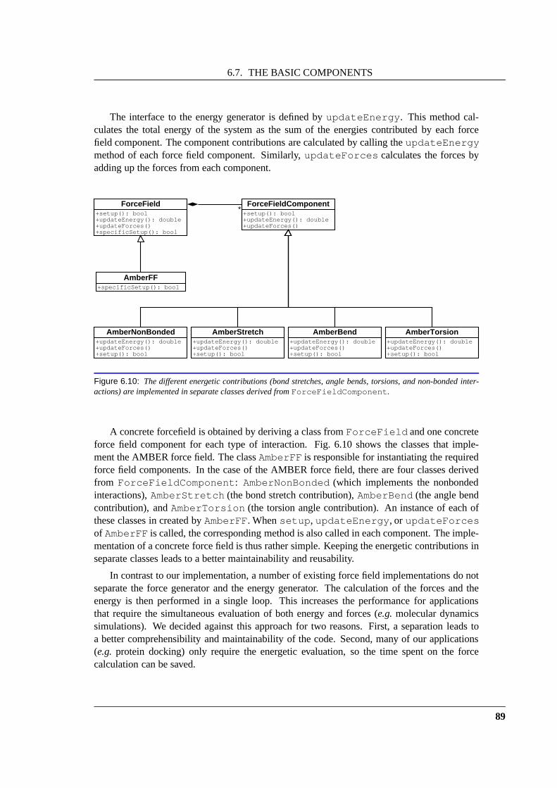
6.7. THE BASIC COMPONENTS
The interface to the energy generator is defined byupdateEnergy . This method cal-culates the total energy of the system as the sum of the energies contributed by each forcefield component. The component contributions are calculated by calling theupdateEnergymethod of each force field component. Similarly,updateForces calculates the forces byadding up the forces from each component.
ForceField+setup(): bool+updateEnergy(): double+updateForces()+specificSetup(): bool
AmberFF+specificSetup(): bool
ForceFieldComponent+setup(): bool+updateEnergy(): double+updateForces()
AmberNonBonded+updateEnergy(): double+updateForces()+setup(): bool
AmberBend+updateEnergy(): double+updateForces()+setup(): bool
AmberStretch+updateEnergy(): double+updateForces()+setup(): bool
AmberTorsion+updateEnergy(): double+updateForces()+setup(): bool
*
Figure 6.10: The different energetic contributions (bond stretches, angle bends, torsions, and non-bonded inter-actions) are implemented in separate classes derived fromForceFieldComponent.
A concrete forcefield is obtained by deriving a class fromForceField and one concreteforce field component for each type of interaction. Fig. 6.10shows the classes that imple-ment the AMBER force field. The classAmberFF is responsible for instantiating the requiredforce field components. In the case of the AMBER force field, there are four classes derivedfrom ForceFieldComponent : AmberNonBonded (which implements the nonbondedinteractions),AmberStretch (the bond stretch contribution),AmberBend (the angle bendcontribution), andAmberTorsion (the torsion angle contribution). An instance of each ofthese classes in created byAmberFF. Whensetup , updateEnergy , or updateForcesof AmberFF is called, the corresponding method is also called in each component. The imple-mentation of a concrete force field is thus rather simple. Keeping the energetic contributions inseparate classes leads to a better maintainability and reusability.
In contrast to our implementation, a number of existing force field implementations do notseparate the force generator and the energy generator. The calculation of the forces and theenergy is then performed in a single loop. This increases theperformance for applicationsthat require the simultaneous evaluation of both energy andforces (e.g.molecular dynamicssimulations). We decided against this approach for two reasons. First, a separation leads toa better comprehensibility and maintainability of the code. Second, many of our applications(e.g. protein docking) only require the energetic evaluation, sothe time spent on the forcecalculation can be saved.
89

CHAPTER 6. DESIGN AND IMPLEMENTATION
Parameters
+init(): bool+setFilename(name:String)+getFilename(): String
INIFile
ParameterSection+options: Options+extractSection(parameters:Parameters,section_name:String): bool+has(key:String,variable:String): bool+hasVariable(variable:String): bool+getValue(key:String,variable:String): String+getValue(key:Position,variable:Position): String+getNumberOfVariables(): Size+getNumberOfKeys(): Size
LennardJones
+extractSection(parameters:Parameters,section_name:String): bool+hasParameters(I:Atom::Type,J:Atom::Type): bool+getParameters(I:Atom::Type,J:Atom::Type): Values
Figure 6.11: The classes related to the reading of parameter files.Parameters contains an instance ofINI-File which reads the parameter file. An instance ofParameterSection (or one of its derived classes) inter-prets the contents of one of the sections of the file as table-like data. The derived classes ofParameterSectionare able to interpret this data and offer a comfortable interface to access it.
Parameter Assignment
A very tiresome and difficult process is the correct parameter assignment and the conversionof existing parameter files. The original implementors of the force fields usually provide amultitude of different versions of parameter sets that evolved over time. The formats used tostore the parameters are text based and column oriented (FORTRAN style). We decided touse a common file format for all parameter files. This allows usto implement the input/outputroutines for these files independent from the force field. Furthermore, our file format has amuch better readability, the related class automatically creates efficient hash data structures toaccess the data, and allows the storage of different parameter versions in a single file.
Parameter files typically consist of one or more sections of (rather independent) parametertables. For example, a force field defines a set of atom types, of Lennard Jones parameters foreach of these types, of stretch, bend, and torsion parameters. All these data sets are stored indifferent sections of a single file.
We represent the whole parameter file as an object of classParameters (see Fig. 6.11).This class uses theINIFile class to read the contents of the parameter file, parses the file, andbuilds internal data structures (several hash maps) to access the contents of the file efficiently.At this level, the data is still stored as tables of strings. The interpretation of the data is carriedout by ParameterSection and its subclasses. The data a certain section should hold isspecified in each class and the user may access this data in a convenient format (usually structs).
For the AMBER force field, this parameter file may look as follows:
1 [...]2 [QuadraticBondStretch]3 ver:version key:I key:J value:k value:r0 value:comment4 @unit_k=kcal/mol5 @unit_r0=Angstrom6 ;7 ;8 ; Rev I J k r0 comment9 ; --- --- --- ---------- ---------- --------------------- --
10 1.0 OW HW 553.000 0.95720 "! TIP3P water"
90

6.7. THE BASIC COMPONENTS
11 1.0 HW HW 553.000 1.50000 "TIP3P water"12 1.1 HW HW 553.000 1.51360 "TIP3P water / corrected"13 1.0 C CA 469.000 1.40900 "JCC,7,(1986),230; TYR"14 [...]1516 [LennardJones]17 ver:version key:I value:R value:epsilon18 @unit_R=Angstrom19 @unit_epsilon=kcal/mol20 @format=RE21 ;22 ;23 ; Rev I R epsilon comment24 ; --- --- ---------- ---------- ------------------------ -25 1.0 C0 1.600000 0.100000 " calcium from parm91.dat"26 1.0 MG 1.170000 0.100000 " magnesium from parm91.dat"27 [...]
In this example, we see two different sections of the file (marked ”[QuadraticBondStretch]”and ”[LennardJones]”). Comment lines start with ”;” and areignored by the parser. Linesstarting with ”@” are options lines and are automatically parsed into an options object (whichis a member ofParameterSection ). These options are used to store specific properties ofthe section (e.g.the units of the columns or additional format information).
The data format of each section is defined in the first line of a section (lines 3 and 17) anddefines the columns of the table. In our case, the Lennard Jones section (used to store van derWaals parameters of the AMBER force field) contains five columns: a version number (columnversion ), an atom type (columnI ), the minimum distance (columnR), the minimum energy(columnepsilon ), and a comment. TheParameters class parses all subsequent lines ofthe section according to this format specification (lines 25–27) and builds a table of strings.The atom type columnI is marked as akey in this table, thus theParameters objectalso creates a hash map allowing fast access through this column. The first column is a specialcolumn: it contains a revision number for each of the lines. Lines with greater revision numbersautomatically supercede lines with a lower revision numberand identical keys. However, theolder revisions of a certain parameter set can be accessed explicitly by specifying an explicitversion number. This is an important feature to document theevolution of a parameter set andto access older parameters sets (e.g.for the purpose of comparison).
The order of the columns is irrelevant, the subclasses ofParameterSection only checkwhether the parameters they require are available. For example, theLennardJones class issatisfied with any table offering a key namedtype and two columns namedRandepsilon .This gives the user the freedom to extend or change the formatto suit his purposes. In con-trast to column based FORTRAN-style formats, which are usedby the majority of softwarepackages, our format is very flexible, readable, and robust.
The Parameters class hierarchy gives a very convenient access to arbitraryparameterfiles and thus simplifies the implementation of the parameterassignment tremendously. Usingthese classes, parameter assignment becomes nearly trivial, as the following code excerptsfrom the AMBER force field prove:
1 // an instance of LennardJones is used to parse2 // the corresponding section of the parameter file3 LennardJones LJ_parameters;
91

CHAPTER 6. DESIGN AND IMPLEMENTATION
4 ...5 // parse the Lennard Jones parameter section6 bool result = LJ_parameters.extractSection7 (getForceField()->getParameters(), "LennardJones");89 // check whether we could parse the section correctly
10 if (result == false)11 {12 ... // some error message13 }14 else15 {16 // iterate over all atoms pairs...17 for (...)18 {19 // ...and determine their type20 ...21 Atom::Type I = atom1->getType();22 Atom::Type J = atom2->getType();2324 // retrieve parameters for the atom pair25 if (LJ_parameters.hasParameters(I, J))26 {27 // retrieve the parameters for atom types I and J28 ...29 values = LJ_parameters.getParameters(I, J);30 }31 else32 {33 // we didn’t find parameters - error message34 ....35 }36 }37 }
Energy Minimization
Energy minimization(or geometry optimization) is one of the two main applications of Molec-ular Mechanics. The problem is as follows: given a set of molecules withN atoms, determinethe set of coordinates~ri (x, y, z) for each atom such that the total energyE(~ri) is minimal.Typically, we are not looking for a global optimum but for a local optimum.
The input sizes range from very few atoms (small molecules, ligands) to large proteins withseveral thousand atoms. This optimization problem is typically attacked using gradient basedtechniques like� steepest descent� conjugate gradient� Newton-Raphson� Quasi-Newton
and a multitude of variants of these methods. The method to bechosen heavily depends onthe exact problem case. In some cases (e.g. initial relaxation of a constructed structure) thesimple steepest descent method is the most efficient one, whereas Newton-Raphson is most
92
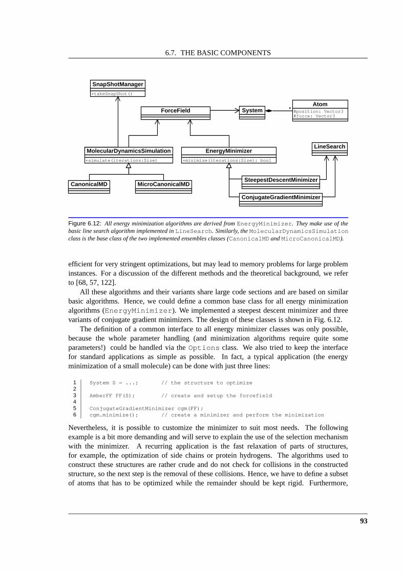
6.7. THE BASIC COMPONENTS
ForceField
EnergyMinimizer
+minimize(iterations:Size): bool
SteepestDescentMinimizer
ConjugateGradientMinimizer
LineSearchMolecularDynamicsSimulation
+simulate(iterations:Size)
CanonicalMD MicroCanonicalMD
SystemAtom
#position: Vector3#force: Vector3
*
SnapShotManager
+takeSnapShot()
Figure 6.12: All energy minimization algorithms are derived fromEnergyMinimizer. They make use of thebasic line search algorithm implemented inLineSearch. Similarly, theMolecularDynamicsSimulationclass is the base class of the two implemented ensembles classes (CanonicalMD andMicroCanonicalMD).
efficient for very stringent optimizations, but may lead to memory problems for large probleminstances. For a discussion of the different methods and thetheoretical background, we referto [68, 57, 122].
All these algorithms and their variants share large code sections and are based on similarbasic algorithms. Hence, we could define a common base class for all energy minimizationalgorithms (EnergyMinimizer ). We implemented a steepest descent minimizer and threevariants of conjugate gradient minimizers. The design of these classes is shown in Fig. 6.12.
The definition of a common interface to all energy minimizer classes was only possible,because the whole parameter handling (and minimization algorithms require quite someparameters!) could be handled via theOptions class. We also tried to keep the interfacefor standard applications as simple as possible. In fact, a typical application (the energyminimization of a small molecule) can be done with just threelines:
1 System S = ...; // the structure to optimize23 AmberFF FF(S); // create and setup the forcefield45 ConjugateGradientMinimizer cgm(FF);6 cgm.minimize(); // create a minimizer and perform the minim ization
Nevertheless, it is possible to customize the minimizer to suit most needs. The followingexample is a bit more demanding and will serve to explain the use of the selection mechanismwith the minimizer. A recurring application is the fast relaxation of parts of structures,for example, the optimization of side chains or protein hydrogens. The algorithms used toconstruct these structures are rather crude and do not checkfor collisions in the constructedstructure, so the next step is the removal of these collisions. Hence, we have to define a subsetof atoms that has to be optimized while the remainder should be kept rigid. Furthermore,
93

CHAPTER 6. DESIGN AND IMPLEMENTATION
we only want to remove the overlaps, so we abort the optimization at a rather large gradient(20 kJ/(molA)):
1 // a protein with unoptimized hydrogen atoms2 System p = ...;34 // setup the force field5 AmberFF FF(p);67 // select the hydrogen atoms only8 Selector H_select("element(H)");9 p.apply(H_select);
1011 // create a minimizer12 StepestDescentMinimizer sdm(FF);1314 // we abort the minimization if the RMS gradient15 // falls below 20 kJ/(mol A)16 sdm.options[EnergyMinimizer::MAX_GRADIENT] = 20.0;17 sdm.minimize();
Molecular Dynamics
The second important application of force fields is theMolecular Dynamics Simulation(MDsimulation, MDS). In an MDS we apply the rules of Newtionian mechanics to the systemdescribed by a Molecular Mechanics force field. By integrating the equations of motion, suc-cessive configurations of the system are generated. Thus, weobtain atrajectory that describeshow the positions of the atoms vary with the time. Again, we have to refer to textbooks for thefundamental theory behind the MDS [38, 68].
MDS trajectories contain a huge amount of interesting information that is closely related toexperimentally accessible data (e.g.diffusion coefficients, radial distribution functions,etc.).So by performing an MD simulation and evaluating the obtained trajectory, we may predictnumerous properties of the system we are investigating.
Depending on the specific problem, we have to decide whichensembleto choose. The termensemble stems from Statistical Thermodynamics and basically describes a collection of a verylarge number of copies of the system whose properties we are investigating. These “copies”differ in their microscopic states, but share the same thermodynamic state (e.g.they share thesame temperatureT , volumeV , and contain the same numberN of particles).
There exists a number of different ensembles that differ by the “experimental conditions” ofthe simulations. In thecanonical ensemble, the number of particles, temperature, and volumeare constant. This corresponds to a set of systems immersed into an infinite bath of temperatureT . While the numberN of particles, volumeV , and temperatureT of each system of theensemble are identical, their energiesE may differ. In contrast to the canonical ensemble, themicrocanonical ensemblerepresents an isolated system whereN , V , andE are constant andTvaries. These two ensembles are the most common ones, so we implemented two classes thatperform MD simulations in a canonical and in a microcanonical ensemble.
The two classesCanonicalMD and MicroCanonicalMD are both derived fromMolecularDynamics and only implement the ensemble dependent part of the code. The
94
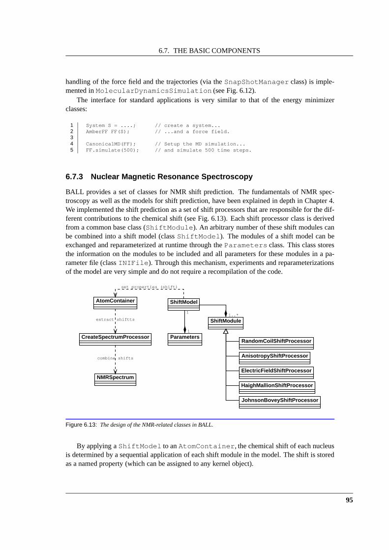
6.7. THE BASIC COMPONENTS
handling of the force field and the trajectories (via theSnapShotManager class) is imple-mented inMolecularDynamicsSimulation (see Fig. 6.12).
The interface for standard applications is very similar to that of the energy minimizerclasses:
1 System S = ....; // create a system...2 AmberFF FF(S); // ...and a force field.34 CanonicalMD(FF); // Setup the MD simulation...5 FF.simulate(500); // and simulate 500 time steps.
6.7.3 Nuclear Magnetic Resonance Spectroscopy
BALL provides a set of classes for NMR shift prediction. The fundamentals of NMR spec-troscopy as well as the models for shift prediction, have been explained in depth in Chapter 4.We implemented the shift prediction as a set of shift processors that are responsible for the dif-ferent contributions to the chemical shift (see Fig. 6.13).Each shift processor class is derivedfrom a common base class (ShiftModule ). An arbitrary number of these shift modules canbe combined into a shift model (classShiftModel ). The modules of a shift model can beexchanged and reparameterized at runtime through theParameters class. This class storesthe information on the modules to be included and all parameters for these modules in a pa-rameter file (classINIFile ). Through this mechanism, experiments and reparameterizationsof the model are very simple and do not require a recompilation of the code.
ShiftModule
RandomCoilShiftProcessor
ElectricFieldShiftProcessor
JohnsonBoveyShiftProcessor
AnisotropyShiftProcessor
HaighMallionShiftProcessor
ShiftModel
1..*
Parameters
1
1
AtomContainer
NMRSpectrum
CreateSpectrumProcessor
set properties (shift)
extract shiftts
combine shifts
Figure 6.13: The design of the NMR-related classes in BALL.
By applying aShiftModel to anAtomContainer , the chemical shift of each nucleusis determined by a sequential application of each shift module in the model. The shift is storedas a named property (which can be assigned to any kernel object).
95

CHAPTER 6. DESIGN AND IMPLEMENTATION
To obtain an NMR spectrum from the assigned chemical shift, we use theCreateSpec-trumProcessor . This class extracts all nuclei with an assigned chemical shift from anAtomContainer object. Then, it discards those atoms that are usually not observable in anNMR spectrum (rapidly exchanging protons), and calculatesthe spectrum as the linear com-bination of Lorentzians (one for each proton). This spectrum is then stored in an instance ofNMRSpectrum. Instances ofNMRSpectrum can be subtracted to give difference spectra,whose areas were used to rank the docking structures in Chapter 4.
6.7.4 Visualization
Introduction
Three-dimensional visualization of molecular structuresis a very important task in MolecularModeling – and a very demanding one as well. In fact, the visualization code is roughlyone sixth of the total BALL code, so a description of this component has to be even moreperfunctory than that of the other components.
Building a framework that allows visualization is very difficult and time-consuming, be-cause it always implies the creation of a graphical user interface (GUI). Writing code that isembedded in a GUI is much more complicated than writing command line applications. Oneway to circumvent this additional labour is the use of an external viewer. This means, we im-plement a typical command line-based program. This programthen either writes its output to afile or directly connects to an external application that visualizes the results. There is a numberof visualization tools available that can be used for this purpose, for example VMD [51] orRasMol [107]. The lack of flexibility is obvious for this approach.
For BALL, we decided to implement a twofold approach:� a comprehensive and powerful framework for the implementation of GUI based applica-tions� a stand-alone viewer used as an external visualization tool, which is based on this frame-work.
The visualization framework is calledBALLVIEW and the external viewer is calledmolview. Since we did not want to implement our own GUI toolkit, we hadto choose one of theexisting packages as a basis for the implementation of BALLVIEW. This GUI toolkit shouldbe portable, object-oriented, written in C++, easy to use, and it should provide the means tovisualize 3D geometric objects. So QT [102] was the only choice. QT is a portable GUI frame-work in C++. It implements all the functionality required to write GUI based applications andalso provides support for the integration of the OpenGL library [86] for 3D rendering.
BALLVIEW itself consists of two distinct frameworks: VIEW and MOLVIEW. While theVIEW framework implements general visualization of arbitrary objects and data, MOLVIEWprovides the specialized models and representations required for the visualization of moleculardata structures. The overall architecture of BALLVIEW is illustrated in Fig. 6.14.
96

6.7. THE BASIC COMPONENTS
QT (GUI tool kit)
OpenGL (3D rendering)
BALLVIEW
MOLVIEW
VIEW
Data Structures Widgets
Renderer/Management
Widgets Processors
Kernel
Foundation Classes
Mathematical DS
Figure 6.14: The overall architecture of the visualization component BALLVIEW (see text).
The VIEW framework
The VIEW framework provides a number of important basic datastructures. First, it definesgeometric primitives, like spheres, tubes, meshes,etc., that are required to describe arbitrarygeometric objects. Second, it defines data types to handle colors and color tables (e.g.to dis-play color-coded gradients or the like). Besides these datastructures, it defines a set of classesto access the OpenGL library. These classes build and managethe display lists required forthe OpenGL renderer. Finally, there is a number ofwidgetsdefined that can be used in appli-cations. Widgets in general are graphical elements (e.g.buttons, text labels,etc.). From thewidget classes of the VIEW framework, we will just introducefour important members: themost important widget is theMainControl widget. It provides the main window for all ap-plications, including a status bar and a menu bar. This widget is usually the central widget thatholds all other widgets. All other widgets are derived from the base classModularWidget .A modular widget can be inserted into the main control and integrates itself automatically. Themechanisms involved are rather complicated, but the effects are simple. The classModular-Widget provides a methodinitializeWidget which is called byMainControl justbefore the widget is to be displayed for the first time. In thismethod, the widget can constructthe menu entries it requires, insert icons or labels into thestatus bar, read its preferences froma global preferences file, or create its own preferences dialog. Each modular widget is thus acomplete prefabricated component and these components canbe combined like building blocksto form an application. The Rapid Application Development capabilities of this approach willbe illustrated by means of an example below.
The third class we will introduce is theScene class. The scene provides three-dimensionalinteractive visualization of geometric objects. The user can rotate, translate, or zoom intothe scene or pick objects by mouse click. This is the key component for three-dimensional
97
CHAPTER 6. DESIGN AND IMPLEMENTATION
visualization of molecular data structures (see Fig. 6.15).The fourth class is theControl , which is used to display the structures contained in a
Scene in a tree-like structure and allows the manipulation and inspection of the contents of ascene (see Fig. 6.15).
The MOLVIEW framework
While the VIEW framework is designed for arbitrary geometric objects, the MOLVIEW frame-work implements the visualization of molecular data structures. This is achieved through a setof processors. These processors can be applied to arbitrarykernel classes and construct a geo-metric representation from it. For example, theAddBallAndStickModel class constructsa ball-and-stick representation from a molecule,i.e. each atom is represented by a sphere andeach bond by a cylinder connecting the two atoms. MOLVIEW provides a number of simi-lar processors for other commonly used models, like the van der Waals models (all atoms asspheres), the line model (all bonds as lines), or molecular surfaces. Similar processors arealso provided to color the resulting representation according to certain properties,e.g.the atomtype, the residue name, the charge,etc.
The MOLVIEW framework also implements specialized variants of several VIEW widgetsthat are aware of molecular data structures and several new modular widgets. For example,there are widgets to read molecular data structures from diverse file formats, widgets that im-plement energy minimizations based on Molecular Mechanicsforce fields, or a widget that canbe applied to add hydrogens to arbitrary structures.
One of the widgets that requires further notice is theServer widget.Server establishesa network socket in the visualization application. Any client application can now create aClient object and connect to that socket. Through the use of object persistence, it is possibleto transmit any kernel data structure to the visualization application. TheServer objectreceives and deserializes the kernel object and displays itdirectly if a Scene is available. Weuse this mechanism for our stand-alone visualization toolmolview , which is explained inmore detail below.
Rapid Application Development using the ModularWidget class
As has been mentioned above, theModularWidget class was developed to simplify therapid construction of applications from some basic building blocks, the modular widgets. Onlythrough the use of the concept of modular widgets, we were able to implement powerful appli-cations with just a few lines of code. The main feature of theModularWidget class is thefact, that each modular widget is self contained and automatically constructs all required con-nections to other widgets. The internal implementation of these features is quite complicated,so we will just discuss the user interface. When developing applications using QT, one usuallyassembles a number of widgets and then implements the behavior of these widgets. For thispurpose, QT uses thesignal-slot mechanism. Signals, as well as slots, are functions (usuallymembers). The signal part is called if a certain action occurs, e.g. if a button is pressed. Byconnecting a certain slot to a signal, the slot is called as soon as the signal isemitted. For exam-ple, pressing the button also calls all connected slots. These slots then implement the required
98

6.7. THE BASIC COMPONENTS
behavior of the interface. These connections are required for menu entries, to connect slidebars to a scrollable view,etc.– the “wiring” of the widgets is usually a very time-consumingand error-prone process.
Modular widgets usually perform this “wiring” automatically. This is achieved by a com-mon, well-defined interface and some internal mechanisms implemented in theMainCon-trol class. Each modular widget defines its own menu entries and the related actions. It mayalso access the application’s status bar via methods ofMainControl . For example, wheninstantiating aOpenPDBFileDialog widget (a widget that reads PDB files), this widgetautomatically creates an entry in File—Import—PDB in the applications menu bar. Clickingon this menu entry allows the selection of a file, which is thenread and a system is created.Now, all relevant widgets have to be informed, that a new system has been read. Using thesignal-slot mechanism for this purpose would be very complicated, so we implemented a sim-ple message passing interface. TheOpenPDBFileDialog widget creates a message statingthat a new system has been read andMainControl distributes this message (along with apointer to the system) to all widgets. Certain modular widgets, like theScene class, interpretthat type of message: the scene displays the system. Other classes simply ignore the message.
These two mechanisms, automatic signal-slot connections and message passing, create anextensible method for widget communication. Combining modular widgets to an applicationthus becomes very simple, as the following code example illustrates. We will implement asimple PDB viewer,i.e.an application that is able to open and to visualize PDB files (as usual,the include directives have been omitted).
1 int main( int argc, char **argv)2 {3 // creating mainframe and application4 QApplication application(argc, argv);5 MainControl mainframe;6 application.setMainWidget(&mainframe);
The main program first creates a QT application, which manages the GUI control flow. Then,we create an instance of theMainControl class and assign it to the main widget of theapplication,i.e. the main control is now the widget that will be displayed in the applicationwindow.
7 QSplitter* splitter = new QSplitter(&mainframe);8 mainframe.setCentralWidget(splitter);9
10 new MolecularControl(splitter);11 new Scene(splitter);1213 new OpenPDBFile(&mainframe);14 new DisplayProperties(&mainframe);15 new MolecularProperties(&mainframe);
Next, we create a splitter, a widget which lets the user control the size of child widgets bydragging the boundary between the children (the vertical bar in Fig. 6.15). We then createthe two child widgets of the splitter: theMolecularControl , which displays kernel datastructures in a tree-like fashion, and theScene , which renders the molecular structures.
In lines 13–15 we create three additional modular widgets:OpenPDBFile is able toread PDB files,DisplayProperties creates the dialog that is used to select one of the
99

CHAPTER 6. DESIGN AND IMPLEMENTATION
different representations for the molecular data structures, andMolecularPropertiesis an (invisible) widget that preprocesses all new kernel data structures, normalizes the atomnames and constructs the bonds between the atoms.
16 // start the application17 mainframe.show();18 return application.exec();19 }
Finally, in lines 17–18 we just start the application. A screenshot of this program in action isgiven in Fig. 6.15.
Figure 6.15: The example code for the MOLVIEW framework in action. There are three widgets visible: theMolecularControl on the left of the splitter, theScene on the right side, and theDisplayPropertiesdialog, which creates the non-modal dialog on the right. TheMolecularControlwidget permits the inspection,selection, and manipulation of kernel data structures. TheScene widget displays these data structures accordingto the representation selected in theDisplayProperties dialog.
The stand-alone viewer molview
Even though the implementation of GUI-based visualizations is rather simple, it is often moreconvenient to write conventional command-line based programs. With the external viewermolview , these applications can then visualize arbitrary molecular data structures with justtwo lines of code:
1 // some system...2 System S = ....;34 // create a client for molview running on host "habakuk"5 Client c("habakuk");67 // send the system and display it on habakuk8 c << S;
100
6.8. SCRIPTING LANGUAGE INTEGRATION
This code creates a client object for the external viewermolview , which is implementedusing the VIEW and the MOLVIEW framework). This client connects to a pre-defined porton a given host (in this case the machinehabakuk ). In the last line of the above example,the client creates a persistent representation of the system, which is then sent to the server (themolview application) using the network streams of BALL. As soon as the server has receivedthe system, it is displayed on the screen. This approach permits the immediate integration ofvisualization capabilities into existing applications. Furthermore, it can be used to separatethe visualization and the calculations. For example, it is possible to execute a computationallyexpensive simulation on a powerful computer server and thenvisualize the result on a graphicsworkstation.
molview also contains functionality to perform energy minimizations using theCHARMM and AMBER force fields, it allows the verification of the structures, the addingof hydrogens, and also an embedded Python interpreter. Thisembedded interpreter providesadditional control over the application, allows the inspection of the data structures, and pro-vides scripting capabilities formolview . The design and implementation of the scriptinglanguage integration is described in detail in the next section.
6.8 Scripting Language Integration
One possibility to speed up Rapid Software Prototpying evenfurther is the integration of script-ing languages. Being interpreted languages, scripting languages obviate the time-consumingcompile and link stages, thus shortening development timesfor software prototypes drastically.Interpreted languages are an useful alternative if new applications can be constructed from ex-isting building blocks and do not require the implementation of complex or computationallyexpensive algorithms. This assumption is valid for the majority of all applications in the fieldof Molecular Modeling. Especially while optimizing parameters of new methods or adaptingexisting methods to specific application cases, the shorterturn-around times are very helpful.
Furthermore, it should be possible to port code very easily from C++ to the scripting lan-guage and vice versa, thus allowing the prototyping in the scripting language and an easyporting of the final variant to C++ to achieve superior performance.
6.8.1 Python
A vast amount of scripting languages has been developed overthe time for these specific pur-poses. The unix world is currently dominated by three scripting languages: Tcl [95], Perl [123],and Python [121]. Each of these languages has been employed as a scripting language in thefield of Computational Molecular Biology. For example, there are currently two Open Sourceprojects in progress, namely BioPython [13] and BioPerl [12]. Both projects develop code forapplications in the life sciences. However, the focus of these projects is currently on sequence-related algorithms and not on Molecular Modeling.
A detailed discussion of the pros and cons of the three scripting languages would justreiterate well-known arguments. Since all these argumentshave been published, we refer tothe respective publications [112, 96, 100]. We will just mention a few points that made mefavor Python over TCL and Perl. First, Python is the only language that is truly object-oriented
101

CHAPTER 6. DESIGN AND IMPLEMENTATION
(in the sense that it was developed to be object-oriented, incontrast to the half-hearted supportfor objects in Perl). Additionally, its readability and intuitive comprehensibility is much betterthan that of the other two languages. Especially the latter two reasons make it much easier forthe average user to learn Python than TCL or Perl. First, we will briefly illustrate some keyconcepts of Python.
Python1 has been developed by Guido van Rossum since 1990. It is an object-orienteddynamic language that was designed to be extensible and modular. One reason for itsreadability is the fact that Python uses indentation to group statements instead of curly bracesas many other languages do. To illustrate some of the basic language concepts of Pythonconsider the following example:
1 for n in range(2, 10):2 for x in range(2, n):3 if n % x == 0:4 break5 else:6 print n, ’is a prime number’
This simple Python program calculates the prime numbers below 10. The first and obviouspoint to notice is the block indentation. The compulsory indentation of blocks leaves the pro-grammer no choice – he has to indent the program correctly andthe block structure is alwaysobvious. The control structures seem rather familiar to C programmers:if conditions,forloops – there’s just one striking difference: in Python, loop statements may haveelse clausesas well. They are executed if the loop is not aborted via thebreak statement. Thefor loopof Python is quite different from C or Pascal. Whilefor loops in C (or C++) can be forced
to perform a whole range of tricks, the Pythonfor loop has a single purpose: it iterates overall items in asequence object. In the above example, the functionrange creates a sequenceof numbers. Thefor loop then iterates over all elements of this sequence. Sequences areof fundamental importance in Python. They come in several flavors, the most important onesbeing lists (asrange produces), tuples, and strings. All sequence types may contain objectsof arbitrary type since Python is aweakly typedlanguage. Python also provides all standardcontrol statements and several other useful data structures (e.g.dictionaries).
6.8.2 Extending
Python was designed to be easily extensible. This can be donevia so-calledextension modulesthat are written in either C or C++. These extension modules can implement new object typesand functions through an API (Application Programmer’s Interface). The API provides nearlycomplete access to the Python interpreter and provides comfortable functions to integrate C orC++ code into the interpreter.
A BALL extension module should provide access to the major part of BALL’s functionalityfrom the Python interpreter and a seamless integration of the BALL objects. The syntax ofthe extension module should be as similar to the C++ syntax as possible. This allows a fast
1Python’s not named after some reptile but afterMonty Python’s Flying Circus– the BBC comedy series Guidovan Rossum obviously enjoyed.
102

6.8. SCRIPTING LANGUAGE INTEGRATION
development of a new method and its refinement in Python and finally – with minor changesonly – the implementation of this code in C++ for extensive experiments and production use.
Although both languages are object-oriented, there are some fundamental differences andconcepts that make these goals rather difficult to meet. The most important topic is genericprogramming using templates. Since the creation of template code always requires a run ofthe C++ compiler, it is not possible to create new instances of templates from the inside of thePython runtime system. Another problem concerns operator overloading: the current releaseof Python does not yet support compound assignment operators (+=, -= , etc.).
The fact that Python functions may not modify the arguments of a called function if theyare immutable(as strings are in Python), is problematic as well. Since BALL often passesreferences of objects to retrieve partial results of a calculation, there are some cases where theinterface had to be changed. In these cases, all return values are passed as a Pythontuple .However, these changes have to be documented and the code cannot be generated automat-ically, so future versions of BALL will avoid passing non-const object references whereverpossible.
The integration of BALL classes into a Python interpreter requires the implementation ofso-calledwrapper classes. Wrapper classes are Python classes that replicate the interface of theC++ class. The methods of these classes call their C++ counterparts and pass the C++ returnvalues back to the Python code. In addition, they have to convert the arguments and returnvalues from C++ objects and types to Python objects and types. Due to the large number ofclasses in BALL, it is obvious that the generation of the wrapper classes has to be automated.There is actually a number of tools available for this purpose. We had a look atSWIG[8],CXX[27], andSIP [116]. Out of these three,SIP was best suited for our purpose. It createsthe wrapper classes from slightly modified BALL header files.
Nevertheless,SIP did not fulfill all requirements. Therefore, we had to modifyit to suitour needs. We added support for C++ operators, meaning that all operators that are supportedby Python are automatically converted to equivalent Pythonmethods. Similarly, exceptionsare translated to Python exceptions. The latter feature requires all C++ methods to declare theexceptions thrown using thethrow keyword.
It was also necessary to find replacements for some concepts used in BALL. For example,iterators are not easily ported to Python. The corresponding concept in Python is the iterationover a sequence (via afor loop). Hence, I created so-calledextractors. Extractors arefunctions that iterate over C++ container objects and assemble a Python sequence containingthese objects (or more precisely: reference to these objects). There exists an extractor for eachkernel iterator type. For example, the C++ code
1 System S = ...;23 AtomIterator ai = S.beginAtom();4 for (; ai != S.endAtom(); ++ai)5 cout << ai->getName() << endl;
translates to the following Python code which uses the extractor atoms :
1 S = ....23 for atom in atoms(S):
103
CHAPTER 6. DESIGN AND IMPLEMENTATION
4 print atom.getName()
Using these techniques we obtained Python extensions that map the BALL functionality andinterface as closely as possible to the corresponding BALL classes and functions. Althoughthere are still some problems to solve (passing of non-constreferences, several unimplementedoperators), the Python extensions have proven to be very helpful when prototyping or debug-ging small to medium scale applications.
6.8.3 Embedding
Embeddingis quite similar to extending Python. The main difference lies in the main program.When using Python extensions, the main application is the Python interpreter that calls BALLcode. When embedding Python, the main application is a BALL program that calls the Pythoninterpreter to execute short code segments. Embedding is required if Python shall be usedas a scripting language inside BALL applications (e.g. for the molecule viewermolview ).A further advantage of an embedded interpreter is the ability to inspect and modify the datainteractively.
There are two design problems related to Python embedding. The first one is the integrationof the interpreter main loop which that to be called as soon asa new code fragment should beexecuted. Since the C API of Python is rather complicated, this should be well hidden behinda more comfortable C++ interface.
The second issue is somehow more difficult. The interpreter has to have access to the appli-cation’s data structures. So we need a way to define which object instances of the applicationmay be accessed from the interpreter and vice versa. This is done via theEmbeddable class.All instances of classes derived fromEmbeddable inherit the membersregisterThisandunregisterThis . By callingregisterThis , a class instance registers with a globalobjects repository (static members ofEmbeddable ). Through the Python bindings of eachclass, the Python interpreter has access to all registered instances.
The following example shall illustrate the interaction of the classes a bit further (alongwith Fig. 6.16).
1 class MyClass2 : public Embeddable3 {4 public:5 BALL_EMBEDDABLE(MyClass)67 MyClass( const String& identifier)8 : Embeddable(identifier)9 {
10 }1112 void print()13 {14 cout << getIdentifier() << endl;15 }16 };
This simple class defines just one trivial method (print ) to print its identifier (which is de-fined byEmbeddable ). The macroBALL EMBEDDABLEdefines the virtual methodreg-
104

6.8. SCRIPTING LANGUAGE INTEGRATION
Embeddable-identifier: String+Embeddable(identifier:String)+~Embeddable()+registerThis()+unregisterThis()+setIdentifier(identifier:String)+getIdentifier(): String
MyClass
+countInstances(): int+getInstance(identifier:String): MyClass*+print()
sipEmbeddable
MyClass [Python]
+countInstances(): int+getInstance(identifier:string): MyClass+print()
Embeddable [Python]
+Embeddable(identifier:String)+~Embeddable()+registerThis()+unregisterThis()+setIdentifier(identifier:String)+getIdentifier(): String
sipMyClass
Figure 6.16: The classEmbeddable is the base class of our classMyClass. For both classes, wrapper classes(sipEmbeddable andsipMyClass ) are automatically created for the Python bindings. Through these inter-mediate classes, Python classesEmbeddable andMyClass have access to the members of the respective BALLclasses.
isterThis that is used to register class instances with the global object repository and thestatic methodsgetInstance andcountInstances . The latter methods can be used toaccess the global instances from Python. The constructor requires a string that is used as aglobal identifier to access this instance (see below).
Now we create an instance of this class in an application (which should contain anembedded Python interpreter) and register it:
1 MyClass my_instance("TESTINSTANCE");2 my_instance.registerThis();
If a Python wrapper was defined for our class and the corresponding module was imported, wecan access our instance from the embedded interpreter via its identifier:
1 >>> MyClass.countInstances()2 13 >>> instance = MyClass.getInstance("TESTINSTANCE")4 >>> instance5 <BALL.MyClass instance at 107cd8>6 >>> instance. print()7 TESTINSTANCE8 >>>
The Embeddable class defines a very simple but very general interface. Special care hasto be taken which methods of these objects can be safely called and who is responsible forthe destruction of a certain instance to avoid memory leaks.Obviously, this interface leaves
105

CHAPTER 6. DESIGN AND IMPLEMENTATION
much room for improvement, but it allows us to embed Python interpreters in applications likemolview in shortest time and with little overhead.
106

Chapter 7
Project Management
This section briefly describes some techniques that were employed to manage the developmentof BALL and to ensure a high quality of the software. In Section 7.1, we will give a descriptionof the methods to keep track of source code changes, revisionmanagement, and portabilityissues. Section 7.4 describes the integrated documentation, Section 7.5 describes the methodswe use for software testing. Finally, in Section 7.6, we willdescribe the mechanisms requiredfor an automated, portable installation of BALL.
7.1 Revision Management
We used theConcurrent Revision System(CVS, [24]) to keep track of source code changes.This was especially important in the beginning, when several people were simultaneouslyworking on the core library. CVS keeps all files in a central repository and stores the changesbetween different versions as context diffs. Even if two or more people are working on a singlefile in parallel, CVS is usually able to merge the changes intoone version of the file – conflictsarise only if the same code lines were changed by different authors. In this case, the respectiveauthor is notified of the conflict and has to resolve it manually.
7.2 Coding Conventions and Software Metrics
The programming style affects the readability of a program.Hence, to ensure a high code qual-ity and a uniform look of the code, we drafted a set of coding conventions. Coding style is avery personal matter and many different styles exist even among the programmers who workedon BALL. An even larger amount of coding styles has been proposed by various authors (e.g.[91, 77, 6]). We drafted a minimal set of non-controversial rules that guarantee a good read-ability without restricting the individual programmer toomuch. They are part of a documentdescribing coding conventions for BALL [63]. Part of these rules is also anorthodox canonicalclass interface[21] that ensures that all BALL classes can be assigned, compared, and copyconstructed. This common interface ensures that all BALL classes can be used in the same wayas typical builtin data types.
However, adhering to these rules is rather inconvenient andcompliance with these rulescould not be reached without enforcement. Several of the rules in the coding conventions canbe verified usingsoftware metrics(or style metrics). Different approaches for style metricshave been proposed in the literature (e.g.[10, 49, 19]) for procedural programming languagesas well as for OO languages.
The open source software packageCCCC (C and C++ Code Counter) [72] provides areasonable choice of different metrics and a WWW-based interface that was easily adoptable

CHAPTER 7. PROJECT MANAGEMENT
to suit our needs. The metrics we used wereLOC (lines of code), COM (comment lines), theirquotient (L C= COMLOC ), and McCabe’scyclomatic complexity[75].
As with the test builds, an overview of the metrics is createdautomatically. Its main purposeis to point out design and implementation flaws in the code. The regular inspection of themetrics helps to identify undocumented code portions and too complex (often poorly designed)classes.
7.3 Portability
The current ANSI standard for C++ was passed in September 1998 as the ISO/IEC standard14882 [5]. However, even today lots of C++ compilers are not fully compliant to this stan-dard. This caused a lot of trouble in the earlier stages of thedevelopment. Nevertheless, thistrouble paid off in the last few months, when more and more compilers were released that aresufficiently close to the ANSI standard to accept our code without major modifications.
7.4 Documentation
7.4.1 Reference Manual and Tutorial
As has been claimed in Section 6.2, documentation is very important for the user. Our goalwas a detailed documentation consistent with the implementation. Therefore, we decided tointegrate the documentation into the BALL source code files and use DOC++ [133] to createprinted and hypertext manuals from the header files. In this way, the documentation alwaysreflects the current state of the implementation. Unlike other approaches, such asCWEB[61],sources documented with DOC++ are ready to be compiled without need of any preprocessing(like tangle ). DOC++ uses a (high-level) C++ parser to extract the documentation fromthe header files. Since this parser reads the class declarations as well, DOC++ is able to createinformation on class hierarchies, member protection, parameters, or return types automatically.The documentation is embedded into special C++ comments starting with ‘/** ’ or ‘ /// ’,hence the code may be compiled directly without modification.
A typical class documentation might look as follows:1 /** Example class.2 This class is meant as an example.\\3 Embedding of LaTeX: $aˆ2 = bˆ2 + cˆ2$\\4 {\bf Definition:}\URL{BALL/test.h}5 \\6 */7 class A8 : public B9 {
10 public:11 /** @name Constructors and Destructor12 */13 //@{14 /** Default constructor15 */16 A();17 //@}18
108

7.5. TESTING
19 /** @name Accessors20 */21 //@{2223 /** Example member.24 This method is useless.25 @param x some number26 @return int the value of the internal attribute divided by {\ tt x}27 @exception DivisionByZero if {\tt x == 0}28 */29 int member( float x) const;30 //@}3132 protected:33 int attribute1;34 };
From this class definition, DOC++ extracts the full documentation in either HTML or LATEXformat. It allows the embedding of LATEX commands as well as the use of several HTML tags.Even mathematical formulas are rendered using LATEX and embedded as GIF images into theHTML page (similar to LaTeX2HTML [26]).
Using the special commands ‘//@ f’ and ‘//@ g’, the members of a class or sections ofthe documentation can be arranged hierarchically. The class hierarchy is represented as classgraphs in the LATEX documentation and as a Java applet in the HTML documentation. A screen-shot of the resulting HTML documentation, including the class graph, is given in Fig. 7.1 onpage 110.
The document resulting from this integrated documentationis the BALL reference manual.It contains detailed descriptions of all classes, their methods and attributes, and references onthe algorithms and models used in the implementation. The reference manual is complementedby a tutorial, which introduces the most important conceptsand classes by means of selectedexample applications.
7.4.2 FAQs
Another part of the documentation is aFAQ list (frequently asked questions). A FAQ list helpsthe user to resolve common problems. Uwe Brahm implemented the BALL FAQ list similarlyto the LEDA FAQ as a Lotus Notes database. We also included theFAQs into the BALLtutorial, because they are most helpful when a user does his first steps with BALL. To keepboth versions consistent, the Notes database is exported regularly in ASCII format, convertedto LATEX, and integrated into the LATEX source code of the tutorial directly.
7.5 Testing
Testing is an important step to ensure the correctness of theimplemented code and is usuallythe last step before releasing the code. Since BALL is a quitelarge project and was alreadyin use while being implemented, we conceived a concept for continuous automatic testing.After introducing some basic terms and definitions in software testing, we will describe thisapproach. For a further discussion of testing and testing techniques, we refer to [56].
109
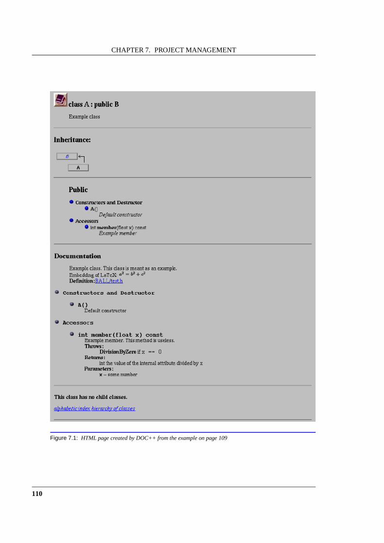
CHAPTER 7. PROJECT MANAGEMENT
Figure 7.1: HTML page created by DOC++ from the example on page 109
110

7.5. TESTING
oracletest
componentin test
testcases comparator test
results
Figure 7.2: General software testing scheme
7.5.1 Fundamentals
The testing of a software component verifies that its behavior complies with a given specifica-tion. For this purpose, a set oftest casesis created and used as an input to the unit in test (seeFig. 7.2). The output of the component is then compared to theoutput of atest oracle. Thetest oracle predicts the outcome for each test case based on the specifications. The componentcomplies to the specification if the results of oracle and thecomponent in test are consideredequal by the comparator for each test case.
Except for some special cases where formal specifications are created during the designphase (e.g.[55]), the generation of the test oracle cannot be automated. Hence, most oraclesare simply humans, usually the ones creating the test cases:while creating a set of test cases,the output for each test case is specified as well. The selection of the test cases depends onwhich approach to testing is used.
There are basically two approaches to testing:black box testing(or functional testingandwhite box testing(or structural testing).
In functional testing, test cases are selected solely on thebasis of the specifications ofthe component. Internals and structure of the component arenot considered. Therefore, it isoften called black box testing. In contrast to black box testing, white box testing considers theinternal structure of the components as well.
7.5.2 Testing in BALL
We decided to use simple black box testing for BALL. The introduction of a testing schemestems from bad experience with the integration of code into the library. Most programmerscontributing code to the project tested their code by writing a small number of short programsthey chose without much thought. As soon as these test programs performed as the programmerexpected (often only on a single platform), the code was submitted to the code repository. Muchlater, sometimes after the programmer had left the project,serious bugs were detected in thecode. Either it did not compile on all platforms due to non portable instructions or headerfiles, or it showed strange behavior for input differing fromthe original test input, or there were
111
CHAPTER 7. PROJECT MANAGEMENT
even syntactically wrong code portions (as might happen forpreviously uninstantiated templatecode).
The testing methods we developed for BALL are rather simple,but proved to be rathereffective. For each class submitted to the code repository,a test program is required. This testprogram has to fulfill the following requirements� it has to test each member of the class� it has to provide a well-defined interface for automatical testing
The first point is especially important for template classes, where code sections are not com-piled if they are not instantiated. Nevertheless, testing of template classes cannot be donesatisfactorily: it is not possible to write tests for each possible template parameter. Further-more, not each method has to be applicable for each template parameter. In these cases, allmembers are tested; each with a single suitable parameter. This method at least ensures thatall code sections are syntactically correct. Then, the methods usually behave correctly for allother suitable template parameters as well.
To ensure a constant software quality, it is not sufficient that a class test once passes onall platforms, but these tests have to be performed on a regular basis on all platforms. Thismay be illustrated by an example. A test for the BALL classObject passed on all platforms.The implementation ofObject relies on the runtime type identification functions (RTTI),for which no test did exist. When the tests for RTTI were implemented, one of these functions(isInstanceOf ) was shown to work incorrectly. Instead of returningtrue if the given objectwas an instance of a certain class, it returnedtrue if this object was ”a kind of” this class. Thus,it replicated the behavior of the functionisKindOf . The error was corrected and the test forthe RTTI then passed on all platforms. However, a subsequenttest of theObject class failed.Obviously, in the implementation ofObject the functionisInstanceOf was used, whereisKindOf was meant. So the removal of an error in one component unveiled an error in acompletely different component.
This example illustrates two important facts. First, it shows the limits of functional testing:theObjects class behaved as specified, although there was an obvious implementation errorthat could have been found by reviewing the code. Second, it shows the importance of repeatedautomatic testing of all classes, since changes in one classoften affect other classes as well.
7.5.3 Test macros
The testing of 460 classes on a dozen platforms has clearly tobe automated. This requires awell defined external interface for all test programs. We decided to implement this as a setof macros. The macros implement a program frame for the classtests. The test of a classor component is broken down into several subtests. Eachsubtestverifies the behavior of onemethod or function and itself consists of severalprimitive tests. In terms of Fig. 7.2, eachmacro represents a primitive test.
What a typical test program might look like is shown in the following listing:
112
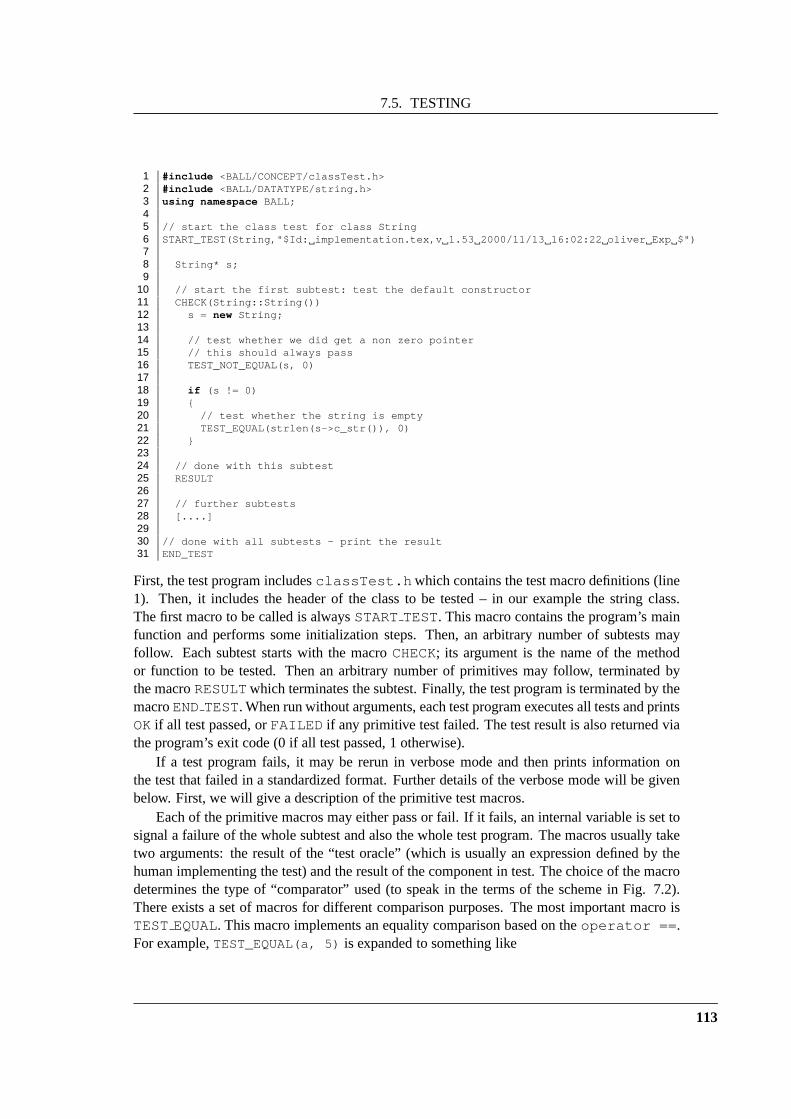
7.5. TESTING
1 #include <BALL/CONCEPT/classTest.h>2 #include <BALL/DATATYPE/string.h>3 using namespace BALL;45 // start the class test for class String6 START_TEST(String,"$Id: implementation.tex,v 1.53 2000/11/13 16:02:22 oliver Exp $")78 String* s;9
10 // start the first subtest: test the default constructor11 CHECK(String::String())12 s = new String;1314 // test whether we did get a non zero pointer15 // this should always pass16 TEST_NOT_EQUAL(s, 0)1718 if (s != 0)19 {20 // test whether the string is empty21 TEST_EQUAL(strlen(s->c_str()), 0)22 }2324 // done with this subtest25 RESULT2627 // further subtests28 [....]2930 // done with all subtests - print the result31 END_TEST
First, the test program includesclassTest.h which contains the test macro definitions (line1). Then, it includes the header of the class to be tested – in our example the string class.The first macro to be called is alwaysSTARTTEST. This macro contains the program’s mainfunction and performs some initialization steps. Then, an arbitrary number of subtests mayfollow. Each subtest starts with the macroCHECK; its argument is the name of the methodor function to be tested. Then an arbitrary number of primitives may follow, terminated bythe macroRESULTwhich terminates the subtest. Finally, the test program is terminated by themacroENDTEST. When run without arguments, each test program executes alltests and printsOKif all test passed, orFAILED if any primitive test failed. The test result is also returned viathe program’s exit code (0 if all test passed, 1 otherwise).
If a test program fails, it may be rerun in verbose mode and then prints information onthe test that failed in a standardized format. Further details of the verbose mode will be givenbelow. First, we will give a description of the primitive test macros.
Each of the primitive macros may either pass or fail. If it fails, an internal variable is set tosignal a failure of the whole subtest and also the whole test program. The macros usually taketwo arguments: the result of the “test oracle” (which is usually an expression defined by thehuman implementing the test) and the result of the componentin test. The choice of the macrodetermines the type of “comparator” used (to speak in the terms of the scheme in Fig. 7.2).There exists a set of macros for different comparison purposes. The most important macro isTEST EQUAL. This macro implements an equality comparison based on theoperator == .For example,TEST_EQUAL(a, 5) is expanded to something like
113

CHAPTER 7. PROJECT MANAGEMENT
bool passed = ((a) == (5));
This macro assumes that the two expressions given are equality comparable,i.e. theopera-tor == has to be defined for the two types.
The opposite behavior is implemented by theTEST NOTEQUALmacro. This primitivetest passes, if the two expressions given as arguments are not equal. This is useful to verifythat a method does not return a null pointer and similar caseswhere only the return value of afailed test may be anticipated.
If the result of a test is a floating point number and deviations from the exact value are tobe expected due to different floating point implementationson different platforms, the macroTEST REALEQUALshould be used. It verifies whether the absolute value of the differencebetween the two arguments is below a user-defined upper bound.
It is also possible to test whether the class’ exception handling behaves as expected. If acertain method should throw an exception, this can be verified using theTEST EXCEPTIONmacro. For example, normalizing a vector of length zero throws a DivisionByZeroexception. A primitive test to verify this behavior might look like this:
1 Vector3 null(0, 0, 0);2 TEST_EXCEPTION(Exception::DivisionByZero, null.norma lize())
This test passes, ifnull.normalize() really throws the exception, which is thencaught by the test macro. Unexpected exceptions are caught automatically by the try/catchblock implemented inCHECKandRESULTif they occur inside a subtest or by the try/catchblock implemented inSTARTTESTandENDTEST if they are thrown outside a subtest. Inany case, the test program fails and a diagnostic message specifying the kind of exceptionthrown is printed in verbose mode.
Finally, theTEST FILE macro is suitable to compare the output written to a file. Forexample, this macro is used to verify the PDB file class which is used to import or exportmolecular structures in the PDB format. In principle, this should be rather simple: read aSystem from disk, write it to a temporary file in PDB format, and compare this file withthe original file. Unfortunately, this approach fails for the very first line of the PDB format:this line contains the date the file was created. This problemis solved by allowing regularexpressions for the files to be compared. The two files are compared line-wise. If a line inthe template file (the “oracle output”) starts with a’/’ , the rest of the line is interpretedas a regular expression and the corresponding line in the temporary file has to match thisexpression. In our example of the PDB class test, the first fewlines of the test output mightlook like this:
1 HEADER BPTI 6-DEC-992 SEQRES 1 58 ARG PRO ASP PHE CYS LEU GLU PRO PRO TYR THR GLY PRO3 SEQRES 2 58 CYS LYS ALA ARG ILE ILE ARG TYR PHE TYR ASN ALA LYS4 SEQRES 3 58 ALA GLY LEU CYS GLN THR PHE VAL TYR GLY GLY CYS ARG5 SEQRES 4 58 ALA LYS ARG ASN ASN PHE LYS SER ALA GLU ASP CYS MET6 SEQRES 5 58 ARG THR CYS GLY GLY ALA
The corresponding lines in the template file are:
1 /HEADER BPTI [ 1-3][0-9]-[A-Z][A-Z][A-Z]-[ 0-9][0-9]2 SEQRES 1 58 ARG PRO ASP PHE CYS LEU GLU PRO PRO TYR THR GLY PRO3 SEQRES 2 58 CYS LYS ALA ARG ILE ILE ARG TYR PHE TYR ASN ALA LYS4 SEQRES 3 58 ALA GLY LEU CYS GLN THR PHE VAL TYR GLY GLY CYS ARG
114
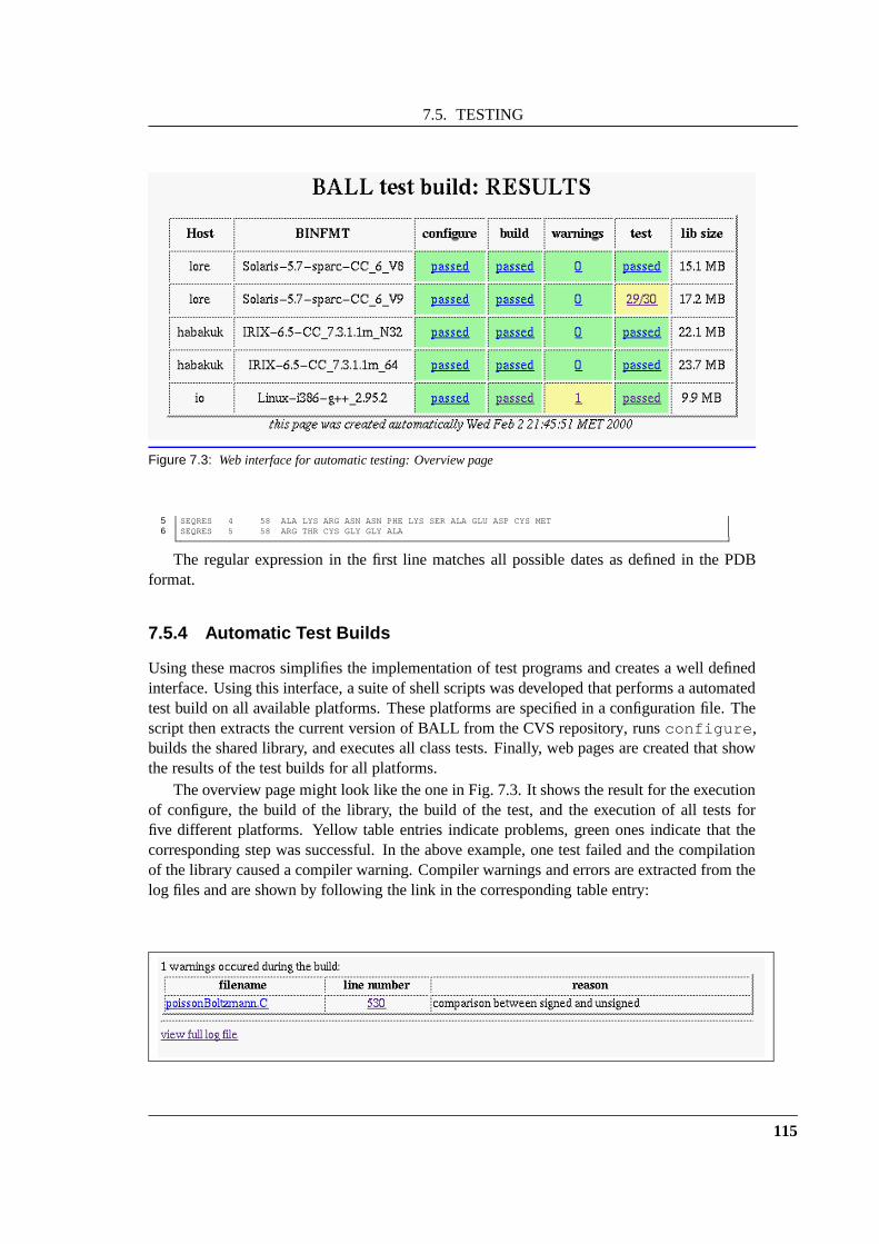
7.5. TESTING
Figure 7.3: Web interface for automatic testing: Overview page
5 SEQRES 4 58 ALA LYS ARG ASN ASN PHE LYS SER ALA GLU ASP CYS MET6 SEQRES 5 58 ARG THR CYS GLY GLY ALA
The regular expression in the first line matches all possibledates as defined in the PDBformat.
7.5.4 Automatic Test Builds
Using these macros simplifies the implementation of test programs and creates a well definedinterface. Using this interface, a suite of shell scripts was developed that performs a automatedtest build on all available platforms. These platforms are specified in a configuration file. Thescript then extracts the current version of BALL from the CVSrepository, runsconfigure ,builds the shared library, and executes all class tests. Finally, web pages are created that showthe results of the test builds for all platforms.
The overview page might look like the one in Fig. 7.3. It showsthe result for the executionof configure, the build of the library, the build of the test, and the execution of all tests forfive different platforms. Yellow table entries indicate problems, green ones indicate that thecorresponding step was successful. In the above example, one test failed and the compilationof the library caused a compiler warning. Compiler warningsand errors are extracted from thelog files and are shown by following the link in the corresponding table entry:
115

CHAPTER 7. PROJECT MANAGEMENT
By following the links for each error, the source code causing the warning can be directlyinspected. The line causing the error is highlighted in red:
This web interface greatly simplifies the maintenance of thecode on all platforms since itimmediately reveals any problems with new code. Since a testbuild is performed every nighton all platforms, committing faulty code to the repository becomes obvious the latest by thenext day. Using the revision control system, a controlled roll back of the software to the lastversion that ran on all platforms can be obtained at any time.
7.6 Installation and Configuration
An important aspect of our design goalease of useis a simple and smooth installation onall required platforms. When we examined existing softwarepackages before we started theimplementation of BALL, installation was a continuous source of frustration. So our goal wasto make the installation of BALL as simple as possible. This is a truly demanding task. First,all platforms are different, all compilers take different options, different versions of softwareor operating system require special workarounds, header files differ from platform to platform,and finally every local installation has its own peculiarities.
116
7.6. INSTALLATION AND CONFIGURATION
GNU autoconf[37] is a portable and extensible tool for the installation of software packets.It uses a very limited set of standard unix tools (sh , ar , sed , etc.) to gather all informationon the system that is required to automatically build and install the libraries. So if everythingworks as expected, a typical installation would only require to run the configuration scriptconfigure and the build the library with the commandmake. configure is a rather com-plex shell script (about 7500 lines long) that identifies theoperating system and the compilerand then searches for the required additional software (e.g.libraries and header files).
Contrary to installation routines that only provide platform dependent configuration files(i.e. a set of files for each combination of operating system and compiler that is supported),configure is based on tests to identify the platforms capabilities. For example, instead ofstating that the GNU compiler does not provide the ANSI classnumerical limits , theconfigure script runs a test program that determines whether thenumerical limitsclass is available. This approach is clearly superior, as itrequires very little effort when portingthe library to a new platform. Most of the porting is done by the configure script whentesting for required features.
Writing these tests in a portable and general way is nevertheless rather tricky and requiresa good knowledge of unix systems and their differences. But this effort usually leads to a veryconvenient installation, as has been shown in our alpha testexperiences. Even if the installationfails, configure provides mechanisms to solve these problems from a distance. For example, theresults of all tests are written to a log file. Usually, by mailing the output of theconfigurescript and this log file, most installation problems can be resolved.
117


Chapter 8
Programming with BALL
In this chapter, we will illustrate the use of BALL for Rapid Software Prototyping by means ofa simple example: the minimization of a protein in vacuum. This example is originally takenfrom the tutorial of the Molecular Modeling package AMBER [22]. To illustrate the differencesbetween a conventional package (AMBER) and BALL, we will contrast the original AMBERcode directly with the BALL code.
The tutorial example performs a conjugate gradient minimization of the protein BPTI invacuum after adding the required hydrogen atoms. Since AMBER is a mere collection ofFORTRAN programs, the code shown here is mainly shell code and input files for the differentFORTRAN programs.
Preparation of the structures
In a first step, we have to add the hydrogen atoms to the BPTI structure, since they areusually not contained in a PDB file. Using AMBER, this is accomplished by theprotonateprogram:
1 protonate -d amber41/dat/PROTON_INFO < pti.pdb > ptiH.pdb
The call to protonate reads the PDB file, adds all missing hydrogens, and stores theinformation to the fileptiH.pdb . In BALL, the same task is accomplished by theadd hydrogens member of the fragment database after reading the PDB file:
1 PDBFile infile("pti.pdb");2 System S;34 infile >> S;56 FragmentDB frag_db;7 S.apply(frag_db.add_hydrogens);
Setting Up the Force Field
Using AMBER, the next step is to establish the topology of theforce field. To achieve this,the programlink is called which reads information on the bonds from a filedat/db4 inthe AMBER data directory (set in the environment variable$AMBERHOME. Prior to the call tolink , an input file has to be constructed that contains the sequence information of the proteinand the necessary information on sulfur bridges:
1 cat <<eof >lnkin2 bpti3

CHAPTER 8. PROGRAMMING WITH BALL
45 DU6 0 0 0 0 07 bpti8 P 1 0 1 3 19 ARG 2PRO ASP PHE CYX LEU GLU PRO PRO TYR THR GLY
10 PRO CYX LYS ALA ARG ILE ILE ARG TYR PHE TYR ASN11 ALA LYS ALA GLY LEU CYX GLN THR PHE VAL TYR GLY12 GLY CYX ARG ALA LYS ARG ASN ASN PHE LYS SER ALA13 GLU ASP CYX MET ARG THR CYX GLY GLY ALA1415 5 55SG SG 016 14 38SG SG 017 30 51SG SG 01819 QUIT20 eof21 #22 link -i lnkin -o lnkout -p $AMBERHOME/dat/db4.dat23 /bin/rm lnkin
The first seven lines contain various configuration flags, that are usually not changed. Ifchanges are done here, one has to be very careful, as the inputformat is strictly column-oriented (as the input formats of most AMBER input files as well), so the number of blanksbefore each number is crucial and blanks and empty lines haveto be counted carefully toavoid unwanted behavior. The next five lines contain the sequence information that has to beextracted from the PDB file manually. Lines 15–17 contain information on the three sulfurbridges of the structure. Again, this information can be extracted from the PDB file. The lasttwo lines finally call link and create the topology information in file lnkout and in the filelinkbin , which is used in the next step by theedit program.
The same code in BALL looks as follows:
8 S.apply(frag_db.build_bonds);
This code constructs all bonds, including the sulfur bridges from the topological informationcontained in the fragment database.
In the next step, AMBER checks the structure of the PDB file forconsistency and writes aset of starting coordinates. This step is carried out using theedit program:
1 cat <<eof > edtin2 bpti3 0 0 0 04 XYZ5 OMIT6 XRAY7 0 0 0 0 08 QUIT9 eof
10 #11 edit -i edtin -o edtout -pi ptiH.pdb12 /bin/rm edtin
This script reads the PDB file fromptiH.pdb , checks it for consistency, and writes startingcoordinates for all atoms toedtout . It also creates an additional file (edtbin ) that contains
120

information on the coordinates and is used in the next step byparm .A similar functionality (although much more sophisticated) is contained in the residue
checker class of BALL. This class exploits the topological and geometric informationcontained in the fragment database to verify the residues itis applied to. Upon failure, it emitsdetailed warning messages.
9 ResidueChecker checker(frag_db);10 S.apply(checker);
In the next step, AMBER reads the information fromedtbin and the force field parameterfile parm91.dat . From these files, it extracts all relevant information on the coordinates, theatom types, and the parameters required for the force field calculation (e.g. force constants,bond lengths,etc.).
1 cat <<eof >prmin2 name of system3 BIN FOR STDA45 067 eof8 #9 parm -i prmin -o prmout -f $AMBERHOME/dat/parm91.dat
10 /bin/rm prmin
Running the Minimization
The minimiztion itself is accomplished by the programsander , which reads the input fromprmtop andprmcrd created in the last step:
1 cat << eof > minin2 # 200 steps of minimization:3 &cntrl4 maxcyc=200, imin=1, cut=12.0, nsnb=20, idiel=0, scee=2.0 , ntpr=10,5 &end6 eof7 sander -i minin -o pti_min.log -c prmcrd -r pti_min.xyz8 /bin/rm minin
This script performs a conjugate gradient minimization fora maximum of 200 steps (givenas the value formaxcyc ). The fact that a full minimization is performed, is specified viathe value ofimin : a value of 1 means a minimization, while a value of 0 starts a MolecularDynamics simulation. The remaining parameters in the fourth line set the parameters for thenonbonded cutoff (cut ) to 12 A, and choose a distance-dependent dielectric constant forthesimulation (idiel=0 ). The current energy during the minimization will be printed every tensteps (nptr=10 ) and the pair list will be updated every 20 steps (nsnb=20 ). The parameterscee specifies a scaling factor for the electrostatic contribution of the force field. The resultingstructure is written to the filepti min.xyz .
In BALL, the code of the last two steps corresponds to the creation of a force field objectand a conjugate gradient minimizer object:
121
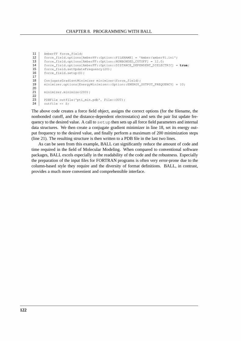
CHAPTER 8. PROGRAMMING WITH BALL
11 AmberFF force_field;12 force_field.options[AmberFF::Option::FILENAME] = "Amb er/amber91.ini";13 force_field.options[AmberFF::Option::NONBONDED_CUTO FF] = 12.0;14 force_field.options[AmberFF::Option::DISTANCE_DEPEN DENT_DIELECTRIC] = true;15 force_field.setUpdateFrequency(20);16 force_field.setup(S);1718 ConjugateGradientMinimizer minimizer(force_field);19 minimizer.options[EnergyMinimizer::Option::ENERGY_O UTPUT_FREQUENCY] = 10;2021 minimizer.minimize(200);2223 PDBFile outfile("pti_min.pdb", File::OUT);24 outfile << S;
The above code creates a force field object, assigns the correct options (for the filename, thenonbonded cutoff, and the distance-dependent electrostatics) and sets the pair list update fre-quency to the desired value. A call tosetup then sets up all force field parameters and internaldata structures. We then create a conjugate gradient minimizer in line 18, set its energy out-put frequency to the desired value, and finally perform a maximum of 200 minimization steps(line 21). The resulting structure is then written to a PDB file in the last two lines.
As can be seen from this example, BALL can significantly reduce the amount of code andtime required in the field of Molecular Modeling. When compared to conventional softwarepackages, BALL excels especially in the readability of the code and the robustness. Especiallythe preparation of the input files for FORTRAN programs is often very error-prone due to thecolumn-based style they require and the diversity of formatdefinitions. BALL, in contrast,provides a much more convenient and comprehensible interface.
122

Chapter 9
Outlook
With BALL, we implemented the first object-oriented framework for Rapid Software Proto-typing in the field of Molecular Modeling. It differs from functionally related packages inits careful design, the use of modern software engineering techniques, and the comprehensivefunctionality. In this section, we will briefly point out some of the current problems and futuredirections for improvement and development.
Most of the current problems are related to the sheer size of the project: BALL containsabout 460 different classes implemented with 270,000 linesof code. An additional 30,000 linesof code implement the class tests. Keeping this amount of code consistent is currently one ofthe major challenges in the development of BALL.
Also the testing of the classes is not yet complete. There aretests implemented for roughlyone third of the classes, so a large number of bugs still awaits discovery. Similarly, there is stilla number of classes with lacking or incomplete documentation. These gaps have to be filled inthe near future as well.
During the alpha test phase, we received extensive feedbackfrom the users. The majority ofthese mails was concerned with requests for additional functionality. It is certainly impossibleto satisfy all the wishes, but there are some key areas that are obviously of general interest. Thefirst field is Molecular Mechanics. Besides the wishes for additional force fields, there is alsoneed for harmonic constraints, and superior optimization methods (quasi-Newton methods,internal coordinate optimization). Second, the visualization component still requires a numberof improvements. Besides additional visualization techniques (e.g.backbone and secondarystructure representations of proteins or mapping of properties onto molecular surfaces), we alsohave to speed up the the visualization component. The Pythonextensions/embedding, althoughalready very useful, does not yet cover all BALL classes and several technical problems relatedto the automatic generation of the wrapper classes remain tobe solved.
Since we intend BALL to become a widely used tool, licenses are free of charge for re-search and teaching, although commercial licenses and support are available as well (throughour partner Algorithmic Solutions Software GmbH). In that way, we hope to resolve some ofthe topics mentioned above in cooperation with other groupsthat are working in the field ofMolecular Modeling.

Part IV
Conclusion

CONCLUSION
In this thesis, we have presented new approaches for the protein docking problem as wellas a comprehensive framework in C++ for rapid software prototyping in the field of MolecularModeling.
Semi-flexible docking
First, we presented two new techniques for semi-flexible protein-protein docking. Based on arigid-body docking algorithm, we developed methods to demangle the amino acid side chainsin the protein-protein interface. This side chain placement problem can be reduced to a com-binatorial optimization problem: identify the set of side chain conformations that yields thelowest energy. The first technique is a so-called multi greedy approach,i.e.we search the enu-meration tree of all possible side chain conformations and avoid combinatorial explosion bylimiting the number of nodes in each layer of the tree to a constant number. The second ap-proach is a branch-&-cut algorithm based on the ILP formulation of the problem. We identifiedseveral classes of facet-defining inequalities and deviseda separation algorithm for a subclassof these inequalities. With the algorithm implemented using BALL, LEDA, and CPLEX, wecould efficiently solve the side chain placement problem optimally. The suboptimal solutionsproduced by the greedy algorithm were sufficiently close to the optimal solutions to give verysimilar results in protein docking: in a test set of three protease-inhibitor complexes, bothmethods were able to correctly demangle the side chains. Theresulting complex structureswere physically meaningful and therefore gave a good ranking in the final energetic evalua-tion step, so both approaches were able to predict the true complex structure for each of thetest cases. Future improvements of the methods could employbranch-&-price techniques onthe algorithmic side or improved energy models and more detailed rotamer libraries on thephysicochemical side.
Use of NMR data for protein docking
Since the energetic evaluation of the docking is a demandingand unsolved problem, we alsotried to identify other possibilities to separate true and false positive complex structures. Wedeveloped an approach that performs this separation based on experimental data. This ap-proach exploits the structural information contained in nuclear magnetic resonance spectraof the complex. Although there have been previous approaches in protein-ligand docking andprotein-protein docking that incorporate NMR data in the form of NOE constraints, our methodis the first method to integrateunmodifiedexperimental data into the docking algorithm. Wedeveloped models and methods to predict the1H-NMR spectra of all tentative complex struc-tures generated by a rigid-body docking algorithm. These spectra were then directly comparedwith the experimental NMR spectrum and the difference area between the two spectra wasused to rank the docking candidates. This approach worked quite well for a set of test casesand was even able to identify the correct complex structure for a very difficult protein-peptidedocking example, where energy-based scoring functions were completely unable to predict thetrue complex structure. This new technique should be applied to a larger set of test cases. Therelevant data is usually not publicly available, but we hopeto get access to that data throughcooperations with NMR research groups. The prediction and comparison of the spectra still
126

CONCLUSION
has lots of room for improvements,e.g.to model hydrogen bonding effects. The technique isapplicable to related problems as well, and thus we hope to beable to speed up NMR-basedstructure elucidation and to transfer our method to the problem of protein structure prediction.
BALL
The above mentioned methods were developed using the BALL framework. BALL is the firstobject-oriented framework for rapid software prototypingin molecular modeling. It has beencarefully designed to be robust, portable, efficient, and extensible. Besides fundamental datastructures, BALL provides functionality for a number of keyareas in Molecular Modeling.We implemented several molecular mechanics force fields, energy minimization algorithms,molecular dynamics simulations, solvation methods, protein motif search and mapping, three-dimensional visualization, file import/export, and NMR shift prediction. BALL consists ofapproximately 460 different classes and 270,000 lines of code. To improve the library’s rapidprototyping capabilities, we embedded the BALL classes into the object-oriented scriptinglanguage Python. After an application has been developed inPython, it is very simple to portit to C++ for production purposes. The BALL library is available for anumber of operatingsystems and compilers and should be easily portable, as it isimplemented in ANSI C++. BALLhas been used in several labs in Europe and North America in the current alpha test phaseand we hope to release the first beta release to a larger audience soon. There still remain anumber of problems to be addressed, namely the documentation, which needs improvementsand the test suite, which does not yet cover all BALL classes.As soon as these problems havebeen resolved, we will extend the functionality of BALL, especially in the fields of MolecularModeling and Protein Engineering. We intend for BALL to become a public repository forreliable data structures and algorithms in the field of Molecular Modeling.
127


Appendix A
UML Notation
This work uses the Unified Modeling Language (UML) to represent design details of BALL.The class diagrams were drawn according to the UML 1.3 standard [90]. A short introductionto this notation can be found in the book by Martin Fowler [36]. A rather comprehensivereference is the book by Rumbaugh, Jacobson, and Booch [103]who are the original designersof the UML. This appendix gives a short overview of the notation used in Part III. The mostimportant concepts of the UML are also explained in the glossary.
Classes and Objects
A central concept in UML is theclass. A class may containattributesandoperations. Thenotation for a class is a rectangle with the class name on top.The lower part of the rectangleusually contains two sections with the attributes and the operations. Public attributes andoperations are prefixed by “+”, protected ones by “#”, and private ones by a “-” sign. Abstractoperations are typeset in italics. Template classes are marked by an additional box at theirupper right corner that contains the template parameter. Objects (i.e. instances of classes) aredistinguished from classes by the underlined object name and class name.
ClassName+public attribute: type = initial value#protected attribute: type-private attribute: type+operation(parameter:type): return type+abstract operation()
class
TemplateClass+attribute: +operation()
parameter
template class
ClassName
attributes and operationssuppressed
name:class name
object
Relationships
Relationships between objects and classes are representedby different kinds of lines andarrows.Associationsare represented as solid lines and may be adorned with role names, asso-ciation names, and multiplicities (just to name the most important decorations). Associationswithout arrows are bidirectional, whereas associations with an arrow are unidirectional. They
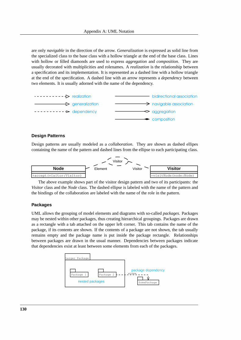
Appendix A: UML Notation
are onlynavigablein the direction of the arrow.Generalizationis expressed as solid line fromthe specialized class to the base class with a hollow triangle at the end of the base class. Lineswith hollow or filled diamonds are used to expressaggregationand composition. They areusually decorated with multiplicities and rolenames. Arealization is the relationship betweena specification and its implementation. It is represented asa dashed line with a hollow triangleat the end of the specification. A dashed line with an arrow represents adependencybetweentwo elements. It is usually adorned with the name of the dependency.
realization
generalization
dependency
bidirectional association
navigable association
aggregation
composition
Design Patterns
Design patterns are usually modeled as acollaboration. They are shown as dashed ellipescontaining the name of the pattern and dashed lines from the ellipse to each participating class.
Visitor
VisitorElementNode
+accept(visitor:Visitor)
Visitor
+visitNode(node:Node)
The above example shows part of the visitor design pattern and two of its participants: theVisitor class and theNodeclass. The dashed ellipse is labeled with the name of the pattern andthe bindings of the collaboration are labeled with the name of the role in the pattern.
Packages
UML allows the grouping of model elements and diagrams with so-calledpackages. Packagesmay be nested within other packages, thus creating hierarchical groupings. Packages are drawnas a rectangle with a tab attached on the upper left corner. This tab contains the name of thepackage, if its contents are shown. If the contents of a package are not shown, the tab usuallyremains empty and the package name is put inside the package rectangle. Relationshipsbetween packages are drawn in the usual manner. Dependencies between packages indicatethat dependencies exist at least between some elements fromeach of the packages.
Larger Package
Package 2Package 1
SomePackage
«use»
nested packages
package dependency
130

Appendix B
Curriculum Vitae
Oliver KohlbacherJohann-Strauß-Straße 1366793 Saarwellingen
Date of Birth 29.08.1971.
Citizenship German.
Education MAX -PLANCK -INSTITUT FUR INFORMATIK SAARBRUCKEN
1996–2000
PhD student.
UNIVERSITAT DES SAARLANDES SAARBRUCKEN
1990–1996
Diplom (�Master’s degree) in Physical Chemistry in 1996. Thesis:ab-initiocalculations of silicate clusters: contributions to the simulation of adsorptionprocesses onSiO2 , advisor: Prof. Dr. Hans Dieter Breuer.
MAX -PLANCK -GYMNASIUM SAARLOUIS
1990
Abitur (� Highschool Diploma).
Work andTeachingExperience I-TRONIX KG SAARBRUCKEN
1999 – present
Geschaftsfuhrer (CEO).
UNIVERSITAT DES SAARLANDES SAARBRUCKEN
1992–1998
Teaching assistant for the following lectures:– Organic Analytics,– Computer Science IV,– Computational Molecular Biology.

Appendix B: Curriculum Vitae
MAX -PLANCK -INSTITUT FUR INFORMATIK SAARBRUCKEN
1992–1996
System administration in the computer service group.
Awards 2000
Heinz Billing Award 2000 for the Advancement of Scientific Computation(for the development of BALL)
Publications
JournalPublications 1. KOHLBACHER, O., AND LENHOF, H.-P. BALL - Rapid Software Proto-
typing in Computational Molecular Biology.Bioinformatics(2000). (inpress).
Book Chapters 2. KOHLBACHER, O. BALL – A Framework for Rapid Application De-velopment in Molecular Modeling. InBeitrage zum Heinz-Billing-Preis2000, no. 55 in Forschung und wissenschaftliches Rechnen - GWDGBerichte. Gesellschaft fur wissenschaftliche Datenverarbeitung mbH,Gottingen, 2000. in press.
ConferencePublications 3. NEUMANN , D., HALTNER, E., LEHR, C.-M., KOHLBACHER, O., AND
LENHOF, H.-P. Investigating the sugar-lectin interaction by computa-tional chemistry: Tunneling the epithelial barrier. InAbstracts of the 18thInterlec Meeting(1998), p. 549.
4. BOGHOSSIAN, N., KOHLBACHER, O.,AND LENHOF, H.-P. BALL: Bio-chemical Algorithms Library. InAlgorithm Engineering, 3rd Interna-tional Workshop, WAE’99, Proceedings(1999), J. Vitter and C. Zaroliagis,Eds., vol. 1668 ofLecture Notes in Computer Science (LNCS), Springer,pp. 330–344.
5. KOHLBACHER, O., AND LENHOF, H.-P. Rapid software prototyping incomputational molecular biology. InProceedings of the German Confer-ence on Bioinformatics (GCB’99)(1999).
6. ALTHAUS, E., KOHLBACHER, O., LENHOF, H.-P., AND M ULLER, P.A combinatorial approach to protein docking with flexible side-chains. InRECOMB 2000 – Proceedings of the Fourth Annual International Confer-ence on Computational Molecular Biology(2000), R. Shamir, S. Miyano,S. Istrail, P. Pevzner, and M. Waterman, Eds., ACM press, pp.15–24.
7. NEUMANN , D., KOHLBACHER, O., HALTNER, E., LENHOF, H.-P.,AND LEHR, C.-M. Modeling the sugar lectin interaction by computa-tional chemistry relevant to drug design. InProc. 3rd World Meeting onPharmaceutics, Biopharmaceutics and Pharmaceutical Technology(Apr2000), p. 233.
132

8. KOHLBACHER, O., BURCHARDT, A., MOLL, A., HILDEBRANDT, A.,BAYER, P.,AND LENHOF, H.-P. A NMR-spectra-based scoring functionfor protein docking. InRECOMB 2001 – Proceedings of the Fifth AnnualInternational Conference on Computational Molecular Biology (2001),D. Sankoff and T. Lengauer, Eds., ACM press. (in press).
TechnicalReports 9. BOGHOSSIAN, N., KOHLBACHER, O.,AND LENHOF, H.-P. BALL: Bio-
chemical Algorithms Library. Tech. Rep. MPI-I-99-1-002, Max-Planck-Institut fur Informatik, Saarbrucken, 1999.
10. ALTHAUS, E., KOHLBACHER, O., LENHOF, H.-P.,AND M ULLER, P. Abranch-and-cut algorithm for the optimal solution of the side-chain place-ment problem. Tech. Rep. MPI-I-2000-1-001, Max-Planck-Institut furInformatik, Saarbrucken, 2000.
Work inProgress 11. ALTHAUS, E., KOHLBACHER, O., LENHOF, H.-P., AND M ULLER, P.
A combinatorial approach to protein docking with flexible side-chains.submitted to J. Comput. Biol, 2000.
12. BOGHOSSIAN, N., KOHLBACHER, O., AND LENHOF, H.-P. Rapid Soft-ware Prototyping in Molecular Modeling using the Biochemical Algo-rithms Library (BALL). submitted to J. Exptl. Algorithmics, 2000.
13. KOHLBACHER, O., BURCHARDT, A., MOLL, A., HILDEBRANDT, A.,BAYER, P., AND LENHOF, H.-P. Structure prediction of protein com-plexes by a NMR-based protein docking algorithm. submittedto J.Biomol. NMR, 2000.
14. NEUMANN , D., KOHLBACHER, O., LENHOF, H.-P.,AND LEHR, C.-M.Protein-sugar interactions: Calculated versus experimental binding ener-gies. submitted to J. Biol. Chem., 2000.
Theses 15. KOHLBACHER, O. ab-initio-Rechnungen an Silikat-Clustern: Unter-suchungen zur Simulation der Adsorption anSiO2. Universitat des Saar-landes. Diplomarbeit, advisor: Prof. Dr. H. D. Breuer, Jan 1996.
133

Appendix C: Bibliography
134
Bibliography
[1] R. Abagyan and M. Totrov. Biased probability Monte Carloconformational searches and electrostatic calculations forpeptides and proteins.J. Mol. Biol., 235:983–1002, 1994.
[2] E. Althaus, O. Kohlbacher, H.-P. Lenhof, and P. Muller.A branch and cut algorithm for the optimal solution of theside–chain placement problem. Technical Report MPI-I-2000-1-001, Max-Planck-Institut fur Informatik, Saarbrucken,2000.
[3] E. Althaus, O. Kohlbacher, H.-P. Lenhof, and P. Muller.A combinatorial approach to protein docking with flexible side–chains. In R. Shamir, S. Miyano, S. Istrail, P. Pevzner, and M. Waterman, editors,RECOMB 2000 – Proceedings of theFourth Annual International Conference on Computational Molecular Biology, pages 15–24. ACM press, 2000.
[4] E. Althaus, O. Kohlbacher, H.-P. Lenhof, and P. Muller.A combinatorial approach to protein docking with flexible side–chains.J. Comput. Biol., 2000. (submitted).
[5] Programming Languages – C++. International Standard, American National Standards Institute, New York, July 1998.Ref. No. ISO/IEC 14882:1998(E).
[6] H. Balzert. Lehrbuch der Software-Technik, volume 2. Spektrum Akakemischer Verlag, 1996.
[7] P. Bayer. personal communication, 2000.
[8] D. M. Beazley. SWIG: An easy to use tool for integrating scripting languages with C and C++. InProceedings of theFourth Annual Tcl/Tk Workshop, pages 129–140. Usenix, 1996.
[9] F. Bernstein, T. Koetzle, G. Williams, E. Meyer Jr, M. Brice, J. Rodgers, O. Kennard, T. Shimanouchi, and M. Tasumi.The protein data bank: a computer-based archival file for macromolecular structures.J. Mol. Biol., 112:535, 1977.
[10] R. E. Berry and B. A. E. Meekings. A style analysis of C programs.Comm. ACM, 28(1):80–88, 1985.
[11] M. J. Betts and M. J. E. Sternberg. An analysis of conformational changes on protein-protein association: implications forpredictive docking.Protein Engineering, 12(4):271–283, 1999.
[12] Bioperl. http://bioperl.org .
[13] Biopython. http://biopython.org .
[14] F. Bloch, W. W. Hansen, and M. E. Packard. Nuclear induction. Phys. Rev., 69:127, 1946.
[15] B. R. Brooks, R. E. Bruccoleri, B. D. Olafson, D. J. States, S. Swaminathan, and M. Karplus. CHARMM: A program formacromolecular energy, minimization, and dynamics calculations.J. Comput. Chem., 4(2):187–217, 1983.
[16] R. E. Bruccoleri and J. Novotny. Antibody modeling using the conformational search program CONGEN.Immunometh-ods, 1:96–106, 1992.
[17] A. D. Buckingham. Chemical shifts in the nuclear magnetic resonance spectra of molecules containing polar groups.Can.J. Chem., 38:300–307, 1960.
[18] W. Chang, I. Shindyalov, C. Pu, and P. Bourne. Design andapplication of PDBLib, a C++ macromolecular class library.CABIOS, 10(6):575–586, 1994.
[19] S. Chidamber and C. Kemerer. Towards a metrics suite forobject oriented design.SIGPLAN Notices, 26(11):197–211,1991.
[20] M. L. Connolly. Shape complementarity at the hemoglobin �1�1 subunit interface.Biopolymers, 25:1229–1247, 1986.
[21] J. O. Coplien.Advanced C++ programming styles and idioms. Addison-Wesley, 1992.

Appendix C: Bibliography
[22] W. D. Cornell, P. Cieplak, C. I. Bayly, I. R. Gould, K. M. Merz Jr., D. M. Ferguson, D. C. Spellmeyer, T. Fox, J. W.Caldwell, and P. A. Kollman. A second generation force field for the simulation of proteins, nucleic acids and organicmolecules.J. Am. Chem. Soc., 117:5179–5197, 1995.
[23] B. Coulange.Software reuse. Springer, London, 1997.
[24] The concurrent versions system.http://www.sourcegear.com/CVS .
[25] J. Desmet, M. D. Maeyer, B. Hazes, and I. Lasters. The dead-end elimination theorem and its use in the protein side-chainpositioning.Nature, 356:539–542, April 1992.
[26] N. Drakos. The LATEX to HTML translator. Technical report, Computer Based Learning Unit, University of Leeds, Jan.1994.
[27] P. Dubois. CXX version 4.2.http://CXX.sourceforge.net/ , 2000.
[28] R. L. Dunbrack and F. E. Cohen. Bayesian statistical analysis of protein side-chain rotamer preferences.Protein Science,6:1661–1681, 1997.
[29] P. Ehrlich. On immunity with special reference to cell life. Proceedings of the Royal Society of London, 66:424–48, 1900.
[30] B. Elshorst, M. Hennig, H. Foersterling, A. Diener, M. Maurer, S. P., H. Schwalbe, C. Griesinger, J. Krebs, H. Schmid,T. Vorherr, and E. Carafoli. NMR solution structure of a complex of calmodulin with a binding peptide of the Ca2+-pump.Biochemistry, 38:12320–12332, 1999.
[31] A. Fabri, G.-J. Giezeman, L. Kettner, S. Schirra, and S.Schonherr. On the design of CGAL, the Computational GeometryAlgorithms Library. Technical Report MPI-I-98-1-007, Max-Planck-Institut fur Informatik, Saarbrucken, Feb. 1998.
[32] D. Fischer, S. L. Lin, H. J. Wolfson, and R. Nussinov. A geometry-based suite of molecular docking processes.J. Mol.Biol., 248:459–477, 1995.
[33] D. Fischer, R. Norel, R. Nussinov, and H. J. Wolfson. 3-Ddocking of protein molecules. InLecture Notes in ComputerScience 684, pages 20–34. Springer Verlag, New York, 1993.
[34] E. Fischer. Einfluss der Konfiguration auf die Wirkung der Enzyme. Berichte der deutschen chemische Gesellschaft,27:2985–2993, 1894.
[35] R. Fleischmann, M. Adams, O. White, E. Kirkness, A. Kerlavage, C. Bult, J. Tomb, B. Dougherty, and J. Merrick. Whole-genome random sequencing and assembly of Haemophilus influenzae Rd.Science, 269(5223):496–512, 1995.
[36] M. Fowler and K. Scott.UML distilled. Addison Wesley, 1997.
[37] Free Software Foundation. GNU autoconf.http://www.gnu.org/software/autoconf/autoconf.html ,2000.
[38] D. Frenkel and B. Smit.Understanding Molecular Simulations. Academic Press, San Diego, CA, 1996.
[39] H. Friebolin. Basic one- and two-dimensional NMR spectroscopy. VCH, Weinheim, 1993.
[40] H. A. Gabb, R. M. Jackson, and M. J. E. Sternberg. Modelling protein docking using shape complementarity, electrostaticsand biochemical information.J. Mol. Biol., 272:106–120, 1997.
[41] E. Gamma, R. Helm, R. Johnson, and J. Vlissides.Design patterns : elements of reusable object-oriented software.Addison-Wesley, Reading, MA, 1995.
[42] M. Goldman.Quantum Description of High-Resolution NMR in Liquids. Oxford University Press, London, 1988.
[43] H. Goldstein.Classical Mechanics. Addison Wesley, 2nd edition, 1980.
[44] M. Gradwell and J. Feeney. Validation of the use of intermolecular NOE constraints for obtaining docked structuresofprotein-ligand complexes.J. Biomol. NMR, 7(1):48–58, 1996.
[45] H. Gunther.NMR-Spektroskopie. Thieme, Stuttgart, 1992.
136

[46] C. W. Haigh and R. B. Mallion. New tables of ring current shielding in proton magnetic resonance.Org. Mag. Res.,4(2):203–228, 1972.
[47] C. W. Haigh and R. B. Mallion. Ring current theories in nuclear magnetic resonance.Prog. NMR. Spec., 13:303–344,1980.
[48] R. K. Harris.Nuclear Magnetic Resonance Spectroscopy. Longman, London, 1994.
[49] W. Harrison and C. Cook. A note on the Berry-Meekings style metric.Comm. ACM, 29(2):123–125, 1986.
[50] L. Holm and C. Sander. Fast and simple monte carlo algorithm for side-chain optimization in proteins: application tomodel building by homology.Proteins, 14:213–223, 1992.
[51] W. Humphrey, A. Dalke, and K. Schulten. VMD – Visual Molecular Dynamics.J. Molecular Graphics, 14:33–38, 1996.
[52] ILOG. ILOG CPLEX 6.5 : user’s manual. ILOG, Bad Homburg, march 1999 edition, 1999.
[53] R. M. Jackson, H. A. Gabb, and M. J. E. Sternberg. Rapid refinement of protein interfaces incorporating solvation:Application to the protein docking problem.J. Mol. Biol., 276:265–285, 1998.
[54] R. M. Jackson and M. J. E. Sternberg. A continuum model for protein-protein interactions: Application to the proteindocking problem.J. Mol. Biol., 250:258–275, 1995.
[55] P. Jalote. Synthesizing implementations of abstract data types from axiomatic specifications.Software Practice andExperience, 17(11):847–858, 1987.
[56] P. Jalote.An integrated approach to software engineering. Undergraduate texts in computer science. Springer, 2nd ed.edition, 1997.
[57] F. Jensen.Introduction to Computational Chemistry. John Wiley & Sons, 1998.
[58] C. E. Johnson and F. A. Bovey.Chem. Phys., 29(5):1012, 1958.
[59] M. Junger and S. Thienel. Introduction to ABACUS - A Branch-And-CUt System. Technical report, Informatik, Universitatzu Koln, 1997.
[60] E. Katchalski-Katzir, I. Shariv, M. Eisenstein, A. A. Friesem, C. Afalo, and I. A. Vakser. Molecular surface recognition:Determination of geometric fit between proteins and their ligands by correlation techniques.Proc. Natl. Acad. Sci. USA,89:2195–2199, 1992.
[61] D. E. Knuth and S. Levy.The CWEB System of Structured Documentation, Version 3.0. Addison-Wesley, Reading, MA,USA, 1993.
[62] P. Koehl and M. Delarue. Application of a self-consistent mean field theory to predict protein side-chains conformationand estimate their conformational entropy.J. Mol. Biol, 239:249–275, 1994.
[63] O. Kohlbacher. BALL Coding Conventions, version 1.1.http://www.mpi-sb.mpg.de/BALL/DOWNLOAD/-coding 1.1.ps , 2000.
[64] D. E. J. Koshland. Application of a theory of enzyme specificity to protein synthesis.Proc. Natl. Acad. Sci. (USA),44:98–104, 1958.
[65] C. A. Laughton. Prediction of protein side-chain conformations from local three-dimensional homology relationships. J.Mol. Biol., 235:1088–1097, 1994.
[66] T. Lazaridis and M. Karplus. Effective energy functionfor proteins in solution.Proteins, 35(2):133–152, 1999.
[67] A. R. Leach. Ligand docking to proteins with discrete side-chain flexibility.J. Mol. Biol., 235:345–356, 1994.
[68] A. R. Leach.Molecular Modeling: Principles and Applications. Addison Wesley Longman, Essex, 1996.
[69] A. R. Leach and A. P. Lemon. Exploring the conformational space of protein side chains using dead-end elimination andthe A* algorithm. Proteins: Struct., Function, and Genet., 33:227–239, 1998.
137

Appendix C: Bibliography
[70] H.-P. Lenhof. An algorithm for the protein docking problem. In D. Schomburg and U. Lessel, editors,Bioinformatics:From nucleic acids and proteins to cell metabolism. GBF Monographs Volume 18, pages 125–139, 1995.
[71] H.-P. Lenhof. New contact measures for the protein docking problem. InProc. of the First Annual International Conferenceon Computational Molecular Biology RECOMB 97, pages 182–191, 1997.
[72] T. Littlefair. C and C++ Code Counter.http://cccc.netpedia.net/ , version 3pre6b, 2000.
[73] R. C. Martin. The interface segregation principle.C++ report, (7), Aug. 1996.
[74] C. K. Mathews and K. van Holde.Biochemistry. The Benjamin/Cummings Publishing Company, 1990.
[75] T. J. McCabe. A complexity measure.IEEE Transactions on Software, 2(4):308–320, 1976.
[76] H. M. McConnell. J. Chem. Phys., 27:227–229, 1957.
[77] S. McConnell.Code Complete: A Practical Handbook of Software Construction. Microsoft Press, 1993.
[78] K. Mehlhorn, S. Naher, M. Seel, and C. Uhrig.The LEDA user manual: version 3.8. Max-Planck-Institut fur Informatik,Saarbrucken, 1999.
[79] B. Meyer. Object-Oriented Software Construction. Prentice Hall PTR, New Jersey, 2nd edition, 1997.
[80] M. Meyer, P. Wilson, and D. Schomburg. Hydrogen bondingand molecular surface shape complementarity as a basis forprotein docking.J. Mol. Biol., 264(1):199–210, 1996.
[81] S. Meyers.Effective C++. Addison-Wesley, Reading, MA, 1998.
[82] X. Morelli, A. Dolla, M. Czjzek, P. N. Palma, F. Blasco, L. Krippahl, J. J. G. Moura, and F. Guerlesquin. HeteronuclearNMR and soft docking: An experimental approach for a structural model of the cytochrome 553-ferredoxin complex.Biochemistry, 39:2530–2537, 2000.
[83] D. R. Musser and A. Saini.STL tutorial and reference guide : C++ programming with the standard template library.Addison-Wesley professional computing ser. Addison-Wesley, Reading, MA, 1996.
[84] D. R. Musser and A. A. Stepanov. Generic programming. InP. Gianni, editor,Proceedings of the International Symposiumon Symbolic and Algebraic Computation, volume 358 ofLNCS, pages 13–25. Springer, 1989.
[85] N. C. Myers. Traits: a new and useful template technique. C++ Report, June 1995.
[86] J. Neider, T. Davis, and M. Woo.OpenGL Programming Guide. Addison–Wesley, Reading, MA, 1993.
[87] G. L. Nemhauser and L. A. Wolsey.Integer and Combinatorial Optimization. Wiley-Interscience Series in DiscreteMathematics and Optimization. Wiley, New York; Chichester; Brisbane, 1988.
[88] A. Nicholls and B. Honig. A rapid finite difference algorithm, utilizing successive over-relaxation to solve the Poisson-Boltzmann equation.J. Comput. Chem., 12(4):435–445, 1991.
[89] R. Norel, S. L. Lin, D. Xu, H. J. Wolfson, and R. Nussinov.Molecular surface variability and induced conformationalchanges upon protein-protein association. In R. H. Sarma and M. H. Sarma, editors,Structure, Motion, Interaction andExpression of Biological Macromolecules. Proceedings of the Tenth Conversation. State University of New York, pages33–51. Adenine Press, 1998.
[90] Object Management Group. Unified modeling language specification, 1998.http://www.omg.org .
[91] P. W. Oman and C. R. Cook. A programming style taxonomy.Journal of Systems and Software, 15(3):287–301, 1991.
[92] K. Osapay and D. Case. Analysis of proton chemical shifts in regular secondary structure of proteins.J. Biomol. NMR,4:215–230, 1994.
[93] K. Osapay and D. A. Case. A new analysis of proton chemical shifts in proteins.J. Am. Chem. Soc., 113:9436–9444, 1991.
[94] M. Osawa, H. Tokumitsu, M. B. Swindells, H. Kurihara, M.Orita, T. Shibanuma, T. Furuya, and M. Ikura. A novelcalmodulin target recognition revealed by its NMR structure in complex with a peptide derived from Ca2+-calmodulin-dependent protein kinase kinase.Nat. Struct. Biol., 6:819, 1999.
138
[95] J. K. Ousterhout.Tcl and the Tk Toolkit. Addison Wesley Publishing Company, 1994.
[96] J. K. Ousterhout. Scripting: Higher level programmingfor the 21st century.Computer, 31(3), 1998.
[97] L. Pauling.Chem. Phys., 4:673, 1936.
[98] V. I. Polshakov, W. D. Morgan, B. Birdsall, and J. Feeney. Validation of a new restraint docking method for solutionstructure determination of protein-ligand complexes.J. Biomol. NMR, 14:115–122, 1999.
[99] J. Ponder and F. Richards. Tertiary templates for proteins – use of packing criteria in the enumeration of allowed sequencesfor different structural classes.J. Mol. Biol., 193:775–791, 1987.
[100] L. Prechelt. An empirical comparison of C, C++, Java, Perl, Python, rexx, and Tcl for a search/string-processing program.Technical Report 2000-5, Universitat Karlsruhe, Fakult¨at fur Informatik, Karlsruhe, Germany, 2000.
[101] E. M. Purcell, H. C. Torrey, and R. V. Pound. Resonance absorption by nuclear magnetic moments in a solid.Phys. Rev.,69:37–38, 1946.
[102] QT release 2.02.http://www.troll.no/products/qt.html .
[103] J. Rumbaugh, I. Jacobson, and G. Booch.The unified modeling language reference manual. Addison Wesley, 1999.
[104] R. R. Rustandi, A. C. Drohat, D. M. Baldisseri, P. T. Wilder, and D. J. Weber. The Ca2+-dependent interaction ofS100B(��) with a peptide derived from p53.Biochemistry, 37:1951–1960, 1998.
[105] B. Sandak, R. Nussinov, and H. J. Wolfson. A Method for Biomolecular Structural Recognition and Docking AllowingConformational Flexibility.J. Comp. Biol., 5(4):631–654, 1998.
[106] B. Sandak, H. J. Wolfson, and R. Nussinov. Flexible Docking Allowing Induced Fit in Proteins: Insights From an OpentoClosed Conformational Isomers.Proteins, 32:159–174, 1998.
[107] R. Sayle and E. Milner-White. RASMOL: biomolecular graphics for all.Trends Biochem. Sci., 20(9):374, 1995.
[108] B. R. Seavey, E. A. Farr, W. M. Westler, and J. Markley. Arelational database for sequence-specific protein NMR data. J.Biomol. NMR, 1:217–236, 1991.
[109] D. Sitkoff, K. A. Sharp, and B. Honig. Accurate calculation of hydration free energies using macroscopic solvent models.J. Phys. Chem., 98(7):1978–1988, 1994.
[110] E. D. Solometsev. Elliptic integral. In M. Hazewinkel, editor,Encyclopedia of Mathematics, volume 3, pages 372–373.Kluwer Academic Publishers, Dordrecht, 1987.
[111] R. Srinivasan.XDR: External Data Representation Standard. Internet Engineering Task Force, 1995. Request for Com-ments 1832.
[112] F. Stajano. Implementing the SMS server, or why I switched from tcl to python. InProceedings of the 7th InternationalPython Conference, Nov. 1998.
[113] M. J. E. Sternberg, H. A. Gabb, and R. M. Jackson. Predictive docking of protein-protein and protein-DNA complexes.Curr. Opin. Struct. Biol., 8:250–256, 1998.
[114] L. Stryer.Biochemie. Spektrum Akademischer Verlag, 1991.
[115] SUN Microsystems.XDR: External Data Representation Standard. Internet Engineering Task Force, Networking WorkingGroup, 1987. Request for Comments 1014.
[116] P. Thompson. Sip version 0.12.http://www.thekompany.com/projects/pykde/ , 2000.
[117] M. Totrov and R. Abagyan. Detailed ab initio prediction of lysozyme-antibody complex with 1.6A accuracy.Nat. Struct.Biol., 1:259–263, 1994.
[118] W. Vahrson, K. Hermann, J. Kleffe, and B. Wittig. Object-oriented sequence analysis: SCL – a C++ class library.CABIOS,12(2):119–127, 1996.
139

Appendix C: Bibliography
[119] I. A. Vakser and C. Aflalo. Hydrophobic docking: a proposed enhancement to molecular recognition techniques.Proteins,20:320–32, 1994.
[120] F. J. M. van de Ven.Multidimensional NMR in liquids: basic principles and experimental methods. Wiley-VCH, NewYork, 1995.
[121] G. van Rossum. Python version 1.5.1.http://www.python.org .
[122] P. von Rague Schleyer, editor.Encyclopedia of Computational Chemistry. John Wiley & Sons, 1998.
[123] L. Wall, T. Christiansen, and R. L. Schwartz.Programming Perl. O’Reilly & Associates Inc., 2nd edition, 1996.
[124] P. Walters and M. Stahl. BABEL version 1.6. Universityof Arizona.
[125] H. Wang. Grid-search molecular accessible surface algorithm for solving the docking problem.J. Comput. Chem., 12:746–750, 1991.
[126] J. S. Waugh and R. W. Fessenden.J. Am. Chem. Soc., 79:846, 1959.
[127] D. J. Weber, A. M. Libson, A. G. Gittis, M. Lebowitz, andA. S. Mildvan. NMR docking of a substrate into the X-raystructure of the ASP-21-GLU mutant of staphylococcal nuclease.Biochemistry, 33(26):8017–8028, 1994.
[128] Z. Weng, S. Vajda, and C. Delisi. Prediction of proteincomplexes using empirical free energy functions.Protein Science,5:614–626, 1996.
[129] M. P. Williamson and T. Asakura. Empirical comparisons of models for chemical-shift calculation in proteins.J. Mag.Res. B, 101:63–71, 1993.
[130] M. P. Williamson, T. Asakura, E. Nakamura, and M. Demura. A method for the calculation of protein�-CH chemicalshifts. J. Biomol. NMR, 2:83–98, 1992.
[131] L. A. Wolsey. Integer programming. Wiley-interscience series in discrete mathematics and optimization. Wiley & Sons,New York, 1998.
[132] C. Zhang, J. L. Cornette, and C. DeLisi. Consistency instructural energetics of protein folding and peptide recognition.Prot. Sci., 6:1059–1064, 1997.
[133] M. Zockler and R. Wunderling. DOC++ version 3.2.http://www.zib.de/Visual/software/doc++/ .
140
Index
Symbols�-helix . . . . . . . . . . . . . . . . . . . . . . . . . . . . . . . . . . . . . . . . . . . . 11�-pleated sheet . . . . . . . . . . . . . . . . . . . . . . . . . . . . . . . . . . . . . 112-deoxyribose . . . . . . . . . . . . . . . . . . . . . . . . . . . . . . . . . . . . . .1480-20 rule . . . . . . . . . . . . . . . . . . . . . . . . . . . . . . . . . . . . . . . . . 69
A
add hydrogens (FragmentDB method) . . . . . . . . . 119AddBallAndStickModel (BALL class) . . . . . . . . . . . 98adenine . . . . . . . . . . . . . . . . . . . . . . . . . . . . . . . . . . . . . . . . . . . .14aggregation . . . . . . . . . . . . . . . . . . . . . . . . . . . . . . . . . . . . . . . 130AMBER . . . . . . . . . . . . . . . . . . . . . . . . . . . . . . . . . . . . . . . 17, 88AmberBend (BALL class) . . . . . . . . . . . . . . . . . . . . . . . . . . 89AmberFF (BALL class) . . . . . . . . . . . . . . . . . . . . . . . . . . . . 89AmberNonBonded (BALL class) . . . . . . . . . . . . . . . . . . . 89AmberStretch (BALL class). . . . . . . . . . . . . . . . . . . . . .89AmberTorsion (BALL class). . . . . . . . . . . . . . . . . . . . . .89amino acids . . . . . . . . . . . . . . . . . . . . . . . . . . . . . . . . . . . . . . . . 10angular momentum quantum number
definition . . . . . . . . . . . . . . . . . . . . . . . . . . . . . . . . . . . . 45ANSI C++ . . . . . . . . . . . . . . . . . . . . . . . . . . . . . . . . . . . . . . . . 70API . . . . . . . . . . . . . . . . . . . . . . . . . . . . . . . . . . . . . . . . . . . . . . 102apply<T> (Composite method) . . . . . . . . . . . . . . . . . . 79ar . . . . . . . . . . . . . . . . . . . . . . . . . . . . . . . . . . . . . . . . . . . . . . . 117association . . . . . . . . . . . . . . . . . . . . . . . . . . . . . . . . . . . . . . . .129Atom (BALL class) . . . . . . . . . . . . . . . . . . . . . . . . . . 67, 76, 84AtomContainer (BALL class) . . . . . . . . . . . . . 85, 95, 96AtomIterator (BALL class). . . . . . . . . . . . . . . . . . . . . .85atoms. . . . . . . . . . . . . . . . . . . . . . . . . . . . . . . . . . . . . . . . . . . . . ..9atoms (PyBALL function) . . . . . . . . . . . . . . . . . . . . . . . . 103AtomVector (BALL class) . . . . . . . . . . . . . . . . . . . . . . . . 88attributes . . . . . . . . . . . . . . . . . . . . . . . . . . . . . . . . . . . . . . . . .129awk . . . . . . . . . . . . . . . . . . . . . . . . . . . . . . . . . . . . . . . . . . . . . . . 82
B
backbone . . . . . . . . . . . . . . . . . . . . . . . . . . . . . . . . . . . . . . . . . . 10BALL . . . . . . . . . . . . . . . . . . . . . . . . . . . . . . . . . . . . . . . . 65–124
AmberFFsetup . . . . . . . . . . . . . . . . . . . . . . . . . . . . . . . . . . 122
CenterOfMassProcessorfinish . . . . . . . . . . . . . . . . . . . . . . . . . . . . . . . . . . 80operator () . . . . . . . . . . . . . . . . . . . . . . . . . . . 80
classesAddBallAndStickModel . . . . . . . . . . . . . . . 98AmberBend . . . . . . . . . . . . . . . . . . . . . . . . . . . . . . 89AmberFF . . . . . . . . . . . . . . . . . . . . . . . . . . . . . . . . . 89AmberNonBonded . . . . . . . . . . . . . . . . . . . . . . . 89AmberStretch . . . . . . . . . . . . . . . . . . . . . . . . . . 89AmberTorsion . . . . . . . . . . . . . . . . . . . . . . . . . . 89Atom . . . . . . . . . . . . . . . . . . . . . . . . . . . . . . 67, 76, 84AtomContainer . . . . . . . . . . . . . . . . . . 85, 95, 96AtomIterator . . . . . . . . . . . . . . . . . . . . . . . . . . 85
AtomVector . . . . . . . . . . . . . . . . . . . . . . . . . . . . . 88CanonicalMD . . . . . . . . . . . . . . . . . . . . . . . . 93, 94CenterOfMassProcessor . . . . . . . . . . 79, 80Chain . . . . . . . . . . . . . . . . . . . . . . . . . . . . . . . . . . . .85Client . . . . . . . . . . . . . . . . . . . . . . . . . . . . . . . . . . 98Composite . . . . . . . . . . . . . . . . . . . . 72, 73, 75, 85composite . . . . . . . . . . . . . . . . . . . . . . . . . . . . . . 72Control . . . . . . . . . . . . . . . . . . . . . . . . . . . . . . . . . 98CreateSpectrumProcessor . . . . . . . . . . . 96DisplayProperties . . . . . . . . . . . . . . . 99, 100DNA. . . . . . . . . . . . . . . . . . . . . . . . . . . . . . . . . . . 67, 85Embeddable . . . . . . . . . . . . . . . . . . . . . . . 104, 105EnergyMinimizer . . . . . . . . . . . . . . . . . . . . . . 93Expression . . . . . . . . . . . . . . . . . . . . . . . . . . . . . 86ExpressionPredicate . . . . . . . . . . . . . . . . 86FDPB. . . . . . . . . . . . . . . . . . . . . . . . . . . . . . . . . . . . . 81ForceField . . . . . . . . . . . . . . . . . . . . . . . . . 88, 89ForceFieldComponent . . . . . . . . . . . . . 88, 89Fragment . . . . . . . . . . . . . . . . . . . . . . . . . . . . 67, 84GeneralException . . . . . . . . . . . . . . . . . . . . .82HINFile . . . . . . . . . . . . . . . . . . . . . . . . . . . . . . . . . 87INIFile . . . . . . . . . . . . . . . . . . . . . . . . . . . . . . . . . 90INIFile . . . . . . . . . . . . . . . . . . . . . . . . . . . . . 90, 95LennardJones . . . . . . . . . . . . . . . . . . . . . . . . . . 91LineSearch . . . . . . . . . . . . . . . . . . . . . . . . . . . . . 93LogStream . . . . . . . . . . . . . . . . . . . . . . . . . . . . . . 81MainControl . . . . . . . . . . . . . . . . . . . . . . . . 97, 99MicroCanonicalMD . . . . . . . . . . . . . . . . . 93, 94ModularWidget . . . . . . . . . . . . . . . . . . . . . 97, 98MOL2File . . . . . . . . . . . . . . . . . . . . . . . . . . . . . . . 87MolecularControl . . . . . . . . . . . . . . . . 99, 100MolecularDynamics . . . . . . . . . . . . . . . . . . . 94MolecularDynamicsSimulation . . 93, 95MolecularProperties . . . . . . . . . . . . . . . 100MolecularStructureFile . . . . . . . . . . . . 87Molecule . . . . . . . . . . . . . . . . . . . . . . . . . 67, 78, 84MyClass . . . . . . . . . . . . . . . . . . . . . . . . . . . . . . . . 105NMRSpectrum . . . . . . . . . . . . . . . . . . . . . . . . . . . 96NucleicAcid . . . . . . . . . . . . . . . . . . . . . . . . . . . 85Nucleotide . . . . . . . . . . . . . . . . . . . . . . . . . . . . . 85Object . . . . . . . . . . . . . . . . . . . . . . . . . . . . . . 74, 112Objects . . . . . . . . . . . . . . . . . . . . . . . . . . . . . . . . 112OpenPDBFile . . . . . . . . . . . . . . . . . . . . . . . . . . . 99OpenPDBFileDialog . . . . . . . . . . . . . . . . . . . 99Options . . . . . . . . . . . . . . . . . . . . . . . . . . 80, 81, 93Parameters . . . . . . . . . . . . . . . . . . . . . . 90, 91, 95ParameterSection . . . . . . . . . . . . . . . . . 90, 91PDBFile . . . . . . . . . . . . . . . . . . . . . . . . . . . . . . . . . 87PersistenceManager . . . . . . . . . . . . . . 74–77PersistentObject . . . . . . . . . . . . . . . . . 74–76Protein . . . . . . . . . . . . . . . . . . . . . . . . . . 67, 78, 85RegularExpression . . . . . . . . . . . . . . . . . . . 82Residue . . . . . . . . . . . . . . . . . . . . . . . . . . . . . . . . . 85ResourceFile . . . . . . . . . . . . . . . . . . . . . . . . . . 87RNA. . . . . . . . . . . . . . . . . . . . . . . . . . . . . . . . . . . 67, 85
INDEX
Scene . . . . . . . . . . . . . . . . . . . . . . . . . . . . . . . 97–100SecondaryStructure . . . . . . . . . . . . . . . . . . 85Selectable . . . . . . . . . . . . . . . . . . . . . . 72, 75, 76Selector . . . . . . . . . . . . . . . . . . . . . . . . . . . . . . . 86Server . . . . . . . . . . . . . . . . . . . . . . . . . . . . . . . . . . 98ShiftModel . . . . . . . . . . . . . . . . . . . . . . . . . . . . . 95ShiftModule . . . . . . . . . . . . . . . . . . . . . . . . . . . 95SnapShotManager . . . . . . . . . . . . . . . . . . . . . . 95SocketStream . . . . . . . . . . . . . . . . . . . . . . . . . . 78String . . . . . . . . . . . . . . . . . . . . . . . . . . . . . . . . . . 82Substring . . . . . . . . . . . . . . . . . . . . . . . . . . . . . . 82System . . . . . . . . . . . . . . . . . . . 67, 84, 85, 87, 114TextPersistenceManager . . . . . . . . . 75–77TimeStamp . . . . . . . . . . . . . . . . . . . . . . . . . . . . . . 73UnaryProcessor<Atom> . . . . . . . . 79, 80, 86UnaryProcessor<T> . . . . . . . . . . . . . . . . . . . 79XDRPersistenceManager . . . . . . . . . . 75, 77XYZFile . . . . . . . . . . . . . . . . . . . . . . . . . . . . . . . . . 87
Compositeapply<T> . . . . . . . . . . . . . . . . . . . . . . . . . . . . . . . 79contains selection . . . . . . . . . . . . . . 72, 73containsSelection . . . . . . . . . . . . . . . . . . . 72
EmbeddablecountInstances . . . . . . . . . . . . . . . . . . . . . . 105getInstance . . . . . . . . . . . . . . . . . . . . . . . . . . 105registerThis . . . . . . . . . . . . . . . . . . . . 104, 105unregisterThis . . . . . . . . . . . . . . . . . . . . . . 104
exceptionsDivisionByZero . . . . . . . . . . . . . . . . . . . . . . 114
FDPBoptions . . . . . . . . . . . . . . . . . . . . . . . . . . . . . . . . . 81
filesclassTest.h . . . . . . . . . . . . . . . . . . . . . . . . . . 113COMMON/global.h . . . . . . . . . . . . . . . . . . . . . . 71config.h . . . . . . . . . . . . . . . . . . . . . . . . . . . . . . . 71
ForceFieldoptions . . . . . . . . . . . . . . . . . . . . . . . . . . . . . . . . . 88setup . . . . . . . . . . . . . . . . . . . . . . . . . . . . . . . . 88, 89updateEnergy . . . . . . . . . . . . . . . . . . . . . . . 88, 89updateForces . . . . . . . . . . . . . . . . . . . . . . . 88, 89
FragmentDBadd hydrogens . . . . . . . . . . . . . . . . . . . . . . . . 119
functionsisInstanceOf . . . . . . . . . . . . . . . . . . . . . . . . . 112isInstanceOf<T> . . . . . . . . . . . . . . . . . . . . . . 78isKindOf . . . . . . . . . . . . . . . . . . . . . . . . . . . . . . 112isKindOf<T> . . . . . . . . . . . . . . . . . . . . . . . . . . . 78
LogStreaminfo . . . . . . . . . . . . . . . . . . . . . . . . . . . . . . . . . . . . . 82setPrefix . . . . . . . . . . . . . . . . . . . . . . . . . . . . . . 82
macrosBALL EMBEDDABLE. . . . . . . . . . . . . . . . . . . . . 104CHECK. . . . . . . . . . . . . . . . . . . . . . . . . . . . . . 113, 114ENDTEST . . . . . . . . . . . . . . . . . . . . . . . . . . 113, 114RESULT. . . . . . . . . . . . . . . . . . . . . . . . . . . . 113, 114STARTTEST. . . . . . . . . . . . . . . . . . . . . . . .113, 114TEST EQUAL. . . . . . . . . . . . . . . . . . . . . . . . . . . . 113TEST EXCEPTION. . . . . . . . . . . . . . . . . . . . . . . 114TEST FILE . . . . . . . . . . . . . . . . . . . . . . . . . . . . . 114TEST NOTEQUAL. . . . . . . . . . . . . . . . . . . . . . . 114TEST REALEQUAL. . . . . . . . . . . . . . . . . . . . . . 114
ModularWidget
initializeWidget . . . . . . . . . . . . . . . . . . . . .97namespaces
Constants . . . . . . . . . . . . . . . . . . . . . . . . . . . . . . 71RTTI . . . . . . . . . . . . . . . . . . . . . . . . . . . . . . . . . . . . . 78
Objectglobal handle . . . . . . . . . . . . . . . . . . . . . . . . 74handle . . . . . . . . . . . . . . . . . . . . . . . . . . . . . . . . . 74
PersistenceManagerget . . . . . . . . . . . . . . . . . . . . . . . . . . . . . . . . . . . . . . 76put . . . . . . . . . . . . . . . . . . . . . . . . . . . . . . . . . . . . . . 76
PersistentObjectfinalize . . . . . . . . . . . . . . . . . . . . . . . . . . . . . . . 74persistentRead . . . . . . . . . . . . . . . . . . . . 74, 76persistentWrite . . . . . . . . . . . . . . . . . . 74, 76read . . . . . . . . . . . . . . . . . . . . . . . . . . . . . . . . . . . . . 76write . . . . . . . . . . . . . . . . . . . . . . . . . . . . . . . . . . . .76
Selectabledeselect . . . . . . . . . . . . . . . . . . . . . . . . . . . . . . . 72select . . . . . . . . . . . . . . . . . . . . . . . . . . . . . . . . . . 72
SystembeginAtom . . . . . . . . . . . . . . . . . . . . . . . . . . . . . . 85endAtom . . . . . . . . . . . . . . . . . . . . . . . . . . . . . . . . . 85
TimeStampstamp . . . . . . . . . . . . . . . . . . . . . . . . . . . . . . . . . . . .73
typesPointerSizeInt . . . . . . . . . . . . . . . . . . . . . . . 71
UnaryOperatoroperator () . . . . . . . . . . . . . . . . . . . . . . . . . . . 86
UnaryProcessor¡T¿finish . . . . . . . . . . . . . . . . . . . . . . . . . . . . . . . . . . 79operator () . . . . . . . . . . . . . . . . . . . . . . . . . . . 79start . . . . . . . . . . . . . . . . . . . . . . . . . . . . . . . . . . . .79
BALL EMBEDDABLE(BALL macro) . . . . . . . . . . . . . . . . 104BALLVIEW
definition . . . . . . . . . . . . . . . . . . . . . . . . . . . . . . . . . . . . 96base . . . . . . . . . . . . . . . . . . . . . . . . . . . . . . . . . . . . . . . . . . . . . . .14base pair . . . . . . . . . . . . . . . . . . . . . . . . . . . . . . . . . . . . . . . . . . .14basic components . . . . . . . . . . . . . . . . . . . . . . . . . . . . . . . . . . . 70beginAtom (System method) . . . . . . . . . . . . . . . . . . . . . 85bend energy . . . . . . . . . . . . . . . . . . . . . . . . . . . . . . . . . . . . . . . . 17big endian . . . . . . . . . . . . . . . . . . . . . . . . . . . . . . . . . . . . . . . . . 77binding site . . . . . . . . . . . . . . . . . . . . . . . . . . . . . . . . . . . . . . . .28biomolecules . . . . . . . . . . . . . . . . . . . . . . . . . . . . . . . . . . . . . . .. 9BioPerl. . . . . . . . . . . . . . . . . . . . . . . . . . . . . . . . . . . . . . . . .5, 101BioPython . . . . . . . . . . . . . . . . . . . . . . . . . . . . . . . . . . . . . . 5, 101black box testing . . . . . . . . . . . . . . . . . . . . . . . . . . . . . . . . . . 111bonded interactions . . . . . . . . . . . . . . . . . . . . . . . . . . . . . . . . .14bovine pancreatic trypsin inhibitor . . . . . . . . . . . . . . . . . . .. . 3BPTI . . . . . . . . . . . . . . . . . . . . . . . . . . . . . . . . . . . . . . . . . . . . . . .3branch-&-cut algorithm . . . . . . . . . . . . . . . . . . . . . . . . . . . . . 29builder . . . . . . . . . . . . . . . . . . . . . . . . . . . . . . . . . . . . . . . . . 74,75
C
C-terminus . . . . . . . . . . . . . . . . . . . . . . . . . . . . . . . . . . . . . . . . .10canonical ensemble
definition . . . . . . . . . . . . . . . . . . . . . . . . . . . . . . . . . . . . 94CanonicalMD (BALL class). . . . . . . . . . . . . . . . . . . .93, 94CCCC. . . . . . . . . . . . . . . . . . . . . . . . . . . . . . . . . . . . . . . . . . . . 107CenterOfMassProcessor (BALL class) . . . . . . 79, 80cerr . . . . . . . . . . . . . . . . . . . . . . . . . . . . . . . . . . . . . . . . . . . . . 81Chain (BALL class) . . . . . . . . . . . . . . . . . . . . . . . . . . . . . . . 85
142

INDEX
chain placement problem . . . . . . . . . . . . . . . . . . . . . . . . . . . . 26CHARMM. . . . . . . . . . . . . . . . . . . . . . . . . . . . . . . . . . . . . . . . .88CHECK(BALL macro) . . . . . . . . . . . . . . . . . . . . . . . . 113, 114chemical bond . . . . . . . . . . . . . . . . . . . . . . . . . . . . . . . . . . . . . . .9chemical shift . . . . . . . . . . . . . . . . . . . . . . . . . . . . . . . . . . . . . .24
definition . . . . . . . . . . . . . . . . . . . . . . . . . . . . . . . . . . . . 48class . . . . . . . . . . . . . . . . . . . . . . . . . . . . . . . . . . . . . . . . . . . . . 129class library . . . . . . . . . . . . . . . . . . . . . . . . . . . . . . . . . . . . . . .. 67classTest.h (BALL file) . . . . . . . . . . . . . . . . . . . . . . . 113Client (BALL class) . . . . . . . . . . . . . . . . . . . . . . . . . . . . . . 98collaboration . . . . . . . . . . . . . . . . . . . . . . . . . . . . . . . . . . . . . .130COM
definition . . . . . . . . . . . . . . . . . . . . . . . . . . . . . . . . . . . 108comment lines
definition . . . . . . . . . . . . . . . . . . . . . . . . . . . . . . . . . . . 108COMMON/global.h (BALL file) . . . . . . . . . . . . . . . . . . . 71Composite (BALL class) . . . . . . . . . . . . . . . 72, 73, 75, 85composite (BALL class) . . . . . . . . . . . . . . . . . . . . . . . . . . 72composite design pattern . . . . . . . . . . . . . . . . . . . . . . . . . . . . 72composition . . . . . . . . . . . . . . . . . . . . . . . . . . . . . . . . . . . . . . 130concrete builder . . . . . . . . . . . . . . . . . . . . . . . . . . . . . . . . . . . .75concrete creator . . . . . . . . . . . . . . . . . . . . . . . . . . . . . . . . . . . .75concrete product . . . . . . . . . . . . . . . . . . . . . . . . . . . . . . . . . . . .75Concurrent Revision System. . . . . . . . . . . . . . . . . . . . . . . . 107config.h (BALL file) . . . . . . . . . . . . . . . . . . . . . . . . . . . . .71configure. . . . . . . . . . . . . . . . . . . . . . . . . . . . . . . . . . . . . 115, 117conjugate gradient . . . . . . . . . . . . . . . . . . . . . . . . . . . . . . . . . .92Constants (BALL namespace) . . . . . . . . . . . . . . . . . . . . 71constraints . . . . . . . . . . . . . . . . . . . . . . . . . . . . . . . . . . . . . . . .. 31contains selection (Composite attribute) 72, 73containsSelection (Composite method) . . . . . . 72continuum model . . . . . . . . . . . . . . . . . . . . . . . . . . . . . . . . . . . 38Control (BALL class) . . . . . . . . . . . . . . . . . . . . . . . . . . . . 98Coulomb’s law . . . . . . . . . . . . . . . . . . . . . . . . . . . . . . . . . . . . . 16countInstances (Embeddable method). . . . . . . .105cout . . . . . . . . . . . . . . . . . . . . . . . . . . . . . . . . . . . . . . . . . . . . . 81CreateSpectrumProcessor (BALL class). . . . . . .96creator . . . . . . . . . . . . . . . . . . . . . . . . . . . . . . . . . . . . . . . . . . . ..75cutting plane . . . . . . . . . . . . . . . . . . . . . . . . . . . . . . . . . . . . . . .32CVS . . . . . . . . . . . . . . . . . . . . . . . . . . . . . . . . . . . . . . . . . 107, 115CWEB . . . . . . . . . . . . . . . . . . . . . . . . . . . . . . . . . . . . . . . . . . . 108CXX. . . . . . . . . . . . . . . . . . . . . . . . . . . . . . . . . . . . . . . . . . . . . . 103cyclomatic complexity . . . . . . . . . . . . . . . . . . . . . . . . . . . . . 108cytosine . . . . . . . . . . . . . . . . . . . . . . . . . . . . . . . . . . . . . . . . . . .14
D
dead-end elimination theorem. . . . . . . . . . . . . . . . . . . . . . . .29deadly diamond
definition . . . . . . . . . . . . . . . . . . . . . . . . . . . . . . . . . . . . 73DEE . . . . . . . . . . . . . . . . . . . . . . . . . . . . . . . . . . . . . . . . . . . . . . 29Democritus of Abdera . . . . . . . . . . . . . . . . . . . . . . . . . . . . . . . . 9deoxyribonucleic acid . . . . . . . . . . . . . . . . . . . . . . . . . . . . . . .13deoxyribose . . . . . . . . . . . . . . . . . . . . . . . . . . . . . . . . . . . . . . . .14dependency . . . . . . . . . . . . . . . . . . . . . . . . . . . . . . . . . . . . . . . 130deselect (Selectable method) . . . . . . . . . . . . . . . . . 72design pattern
composite . . . . . . . . . . . . . . . . . . . . . . . . . . . . . . . . . . . . 72design patterns . . . . . . . . . . . . . . . . . . . . . . . . . . . . . . . . . . . . 130
builder . . . . . . . . . . . . . . . . . . . . . . . . . . . . . . . . . . . . . . . 74definition . . . . . . . . . . . . . . . . . . . . . . . . . . . . . . . . . . . . 68factory method . . . . . . . . . . . . . . . . . . . . . . . . . . . . . . . 74
diffusion coefficients . . . . . . . . . . . . . . . . . . . . . . . . . . . . . . .. 94director . . . . . . . . . . . . . . . . . . . . . . . . . . . . . . . . . . . . . . . . . . .. 75DisplayProperties (BALL class) . . . . . . . . . . 99, 100DivisionByZero (BALL class) . . . . . . . . . . . . . . . . . . 114DNA . . . . . . . . . . . . . . . . . . . . . . . . . . . . . . . . . . . . . . . . . . . . . . 13DNA(BALL class) . . . . . . . . . . . . . . . . . . . . . . . . . . . . . . 67, 85DOC++ . . . . . . . . . . . . . . . . . . . . . . . . . . . . . . . . . . . . . . . . . . 108Docking
protein-protein. . . . . . . . . . . . . . . . . . . . . . . . . . . . . . . .25semi-flexible . . . . . . . . . . . . . . . . . . . . . . . . . . . . . . . . . 25
docking . . . . . . . . . . . . . . . . . . . . . . . . . . . . . . . . . . . . . 19–61, 64flexible . . . . . . . . . . . . . . . . . . . . . . . . . . . . . . . . . . . 25–45
double helix . . . . . . . . . . . . . . . . . . . . . . . . . . . . . . . . . . . . . . . .14drug design . . . . . . . . . . . . . . . . . . . . . . . . . . . . . . . . . . . . . . . . .2dynamiccast . . . . . . . . . . . . . . . . . . . . . . . . . . . . . . . . . . . . . . . 78
E
edit . . . . . . . . . . . . . . . . . . . . . . . . . . . . . . . . . . . . . . . . . . . . 120effective field . . . . . . . . . . . . . . . . . . . . . . . . . . . . . . . . . . . . . .47electron microscopy . . . . . . . . . . . . . . . . . . . . . . . . . . . . . . . . 45electrostatic energy . . . . . . . . . . . . . . . . . . . . . . . . . . . . . . . .. 17Embeddable (BALL class) . . . . . . . . . . . . . . . . . . . 104, 105Embeddable (PyBALL class) . . . . . . . . . . . . . . . . . . . . . 105Embedding . . . . . . . . . . . . . . . . . . . . . . . . . . . . . . . . . . . . . . . 104Emil Fischer . . . . . . . . . . . . . . . . . . . . . . . . . . . . . . . . . . . . . . . .2ENDTEST(BALL macro) . . . . . . . . . . . . . . . . . . . . . 113, 114endAtom (System method) . . . . . . . . . . . . . . . . . . . . . . . . 85energy generator . . . . . . . . . . . . . . . . . . . . . . . . . . . . . . . . . . . .88Energy minimization . . . . . . . . . . . . . . . . . . . . . . . . . . . . . . . . 92EnergyMinimizer (BALL class) . . . . . . . . . . . . . . . . . 93ensemble . . . . . . . . . . . . . . . . . . . . . . . . . . . . . . . . . . . . . . . . . . 94ethanol . . . . . . . . . . . . . . . . . . . . . . . . . . . . . . . . . . . . . . . . . . . .. 9exhaustive search . . . . . . . . . . . . . . . . . . . . . . . . . . . . . . . . . . .26Expression (BALL class) . . . . . . . . . . . . . . . . . . . . . . . . 86ExpressionPredicate (BALL class) . . . . . . . . . . . . 86extension modules . . . . . . . . . . . . . . . . . . . . . . . . . . . . . . . . . 102External Data Representation . . . . . . . . . . . . . . . . . . . . . . . . 77extractors
definition . . . . . . . . . . . . . . . . . . . . . . . . . . . . . . . . . . . 103
F
factory method . . . . . . . . . . . . . . . . . . . . . . . . . . . . . . . . . . . . . 74false positives
definition . . . . . . . . . . . . . . . . . . . . . . . . . . . . . . . . . . . . 21FAQ list . . . . . . . . . . . . . . . . . . . . . . . . . . . . . . . . . . . . . . . . . . 109FDPB(BALL class) . . . . . . . . . . . . . . . . . . . . . . . . . . . . . . . . 81field sweep. . . . . . . . . . . . . . . . . . . . . . . . . . . . . . . . . . . . . . . . .48finalize (PersistentObject method) . . . . . . . . . 74finish (CenterOfMassProcessor method). . . . .80finish (UnaryProcessor<T> attribute) . . . . . . . . . 79finish (UnaryProcessor<T> method) . . . . . . . . . . 79for loop (Python) . . . . . . . . . . . . . . . . . . . . . . . . . . . . . . . . 102force . . . . . . . . . . . . . . . . . . . . . . . . . . . . . . . . . . . . . . . . . . . . . .16force field . . . . . . . . . . . . . . . . . . . . . . . . . . . . . . . . . . . . . . 16, 17force generator . . . . . . . . . . . . . . . . . . . . . . . . . . . . . . . . . . . . .88ForceField (BALL class) . . . . . . . . . . . . . . . . . . . . . 88, 89ForceFieldComponent (BALL class) . . . . . . . . . 88, 89Foundation Classes . . . . . . . . . . . . . . . . . . . . . . . . . . . . . . . . . 70Fourier transform . . . . . . . . . . . . . . . . . . . . . . . . . . . . . . . . . . .45Fragment (BALL class) . . . . . . . . . . . . . . . . . . . . . . . . 67, 84
143

INDEX
framework . . . . . . . . . . . . . . . . . . . . . . . . . . . . . . . . . . . . . . . . . 67frequency sweep. . . . . . . . . . . . . . . . . . . . . . . . . . . . . . . . . . . .49functional testing . . . . . . . . . . . . . . . . . . . . . . . . . . . . . . . . . .111
G
GeneralException (BALL class) . . . . . . . . . . . . . . . . 82generalization . . . . . . . . . . . . . . . . . . . . . . . . . . . . . . . . . . . . .130generic programming
definition . . . . . . . . . . . . . . . . . . . . . . . . . . . . . . . . . . . . 68genomics . . . . . . . . . . . . . . . . . . . . . . . . . . . . . . . . . . . . . . . . . . .2geometry optimization . . . . . . . . . . . . . . . . . . . . . . . . . . . . . . 92get (PersistenceManager method) . . . . . . . . . . . . . 76getInstance (Embeddable method) . . . . . . . . . . . . 105global minimum energy conformation . . . . . . . . . . . . . . . . 26global handle (Object attribute) . . . . . . . . . . . . . . 74GMEC . . . . . . . . . . . . . . . . . . . . . . . . . . . . . . . . . . . . . . . . . . . . 26GMEC polyhedron
definition . . . . . . . . . . . . . . . . . . . . . . . . . . . . . . . . . . . . 32GNU autoconf . . . . . . . . . . . . . . . . . . . . . . . . . . . . . . . . . . . . 117graphical user interface. . . . . . . . . . . . . . . . . . . . . . . . . . . . ..96guanine. . . . . . . . . . . . . . . . . . . . . . . . . . . . . . . . . . . . . . . . . . . .14GUI . . . . . . . . . . . . . . . . . . . . . . . . . . . . . . . . . . . . . . . . . . . . . . . 96Guido van Rossum . . . . . . . . . . . . . . . . . . . . . . . . . . . . . . . . 102gyromagnetic ratio . . . . . . . . . . . . . . . . . . . . . . . . . . . . . . . . . .46
H
Haemophilus influenzae . . . . . . . . . . . . . . . . . . . . . . . . . . . . . . 2handle (Object attribute) . . . . . . . . . . . . . . . . . . . . . . . 74HINFile (BALL class) . . . . . . . . . . . . . . . . . . . . . . . . . . . . 87human genome . . . . . . . . . . . . . . . . . . . . . . . . . . . . . . . . . . . . . . 2hydroxyl group . . . . . . . . . . . . . . . . . . . . . . . . . . . . . . . . . . . . . .9
I
ILP . . . . . . . . . . . . . . . . . . . . . . . . . . . . . . . . . . . . . . . . . . . . . . . 29immutable . . . . . . . . . . . . . . . . . . . . . . . . . . . . . . . . . . . . . . . . 103induced fit . . . . . . . . . . . . . . . . . . . . . . . . . . . . . . . . . . . . . . 19, 21info (LogStream method) . . . . . . . . . . . . . . . . . . . . . . . . 82INIFile (BALL class) . . . . . . . . . . . . . . . . . . . . . . . . . . . . 90INIFile (BALL class) . . . . . . . . . . . . . . . . . . . . . . . . . 90, 95initializeWidget (ModularWidget method) . . 97integer linear program. . . . . . . . . . . . . . . . . . . . . . . . . . . . . . .31Integer Linear Programming . . . . . . . . . . . . . . . . . . . . . . . . . 29interface pollution . . . . . . . . . . . . . . . . . . . . . . . . . . . . . . . . .. 79intermolecular exchange . . . . . . . . . . . . . . . . . . . . . . . . . . . . 53intramolecular interactions . . . . . . . . . . . . . . . . . . . . . . . . .. 14ions
definition . . . . . . . . . . . . . . . . . . . . . . . . . . . . . . . . . . . . 15isInstanceOf (BALL function) . . . . . . . . . . . . . . . . . 112isInstanceOf<T> (BALL function) . . . . . . . . . . . . . . 78isKindOf (BALL function) . . . . . . . . . . . . . . . . . . . . . . . 112isKindOf<T> (BALL function) . . . . . . . . . . . . . . . . . . . . 78isolated system . . . . . . . . . . . . . . . . . . . . . . . . . . . . . . . . . . . . .94iterator traits . . . . . . . . . . . . . . . . . . . . . . . . . . . . . . . . . . . . .. . 79iterators . . . . . . . . . . . . . . . . . . . . . . . . . . . . . . . . . . . . . . . . . .. 79
K
kerneliterators . . . . . . . . . . . . . . . . . . . . . . . . . . . . . . . . . . . . . . 85
kernel classes . . . . . . . . . . . . . . . . . . . . . . . . . . . . . . . . . . . . . .70
L
L Cdefinition . . . . . . . . . . . . . . . . . . . . . . . . . . . . . . . . . . . 108
Larmor frequency . . . . . . . . . . . . . . . . . . . . . . . . . . . . . . . . . . 47Larmor precession
definition . . . . . . . . . . . . . . . . . . . . . . . . . . . . . . . . . . . . 47LennardJones (BALL class). . . . . . . . . . . . . . . . . . . . . .91Leucippus of Miletus. . . . . . . . . . . . . . . . . . . . . . . . . . . . . . . . .9Life Science. . . . . . . . . . . . . . . . . . . . . . . . . . . . . . . . . . . . . . . ..2lines of code
definition . . . . . . . . . . . . . . . . . . . . . . . . . . . . . . . . . . . 108LineSearch (BALL class) . . . . . . . . . . . . . . . . . . . . . . . . 93link . . . . . . . . . . . . . . . . . . . . . . . . . . . . . . . . . . . . . . . . . . . . 119little endian . . . . . . . . . . . . . . . . . . . . . . . . . . . . . . . . . . . . . . .. 77LOC
definition . . . . . . . . . . . . . . . . . . . . . . . . . . . . . . . . . . . 108lock-and-key principle . . . . . . . . . . . . . . . . . . . . . . . . . . . . . .. 2
definition . . . . . . . . . . . . . . . . . . . . . . . . . . . . . . . . . . . . 19LogStream (BALL class) . . . . . . . . . . . . . . . . . . . . . . . . . . 81Lorentzian . . . . . . . . . . . . . . . . . . . . . . . . . . . . . . . . . . . . . . . . .53Lotus Notes . . . . . . . . . . . . . . . . . . . . . . . . . . . . . . . . . . . . . . . 109
M
magnetic moment. . . . . . . . . . . . . . . . . . . . . . . . . . . . . . . . . . .46magnetic quantum number
definition . . . . . . . . . . . . . . . . . . . . . . . . . . . . . . . . . . . . 46MainControl (BALL class). . . . . . . . . . . . . . . . . . . .97, 99methyl group . . . . . . . . . . . . . . . . . . . . . . . . . . . . . . . . . . . . . . . .9microcanonical ensemble
definition . . . . . . . . . . . . . . . . . . . . . . . . . . . . . . . . . . . . 94MicroCanonicalMD (BALL class) . . . . . . . . . . . . . 93, 94MMTK . . . . . . . . . . . . . . . . . . . . . . . . . . . . . . . . . . . . . . . . . . . . . 5ModularWidget (BALL class) . . . . . . . . . . . . . . . . . 97, 98MOL2File (BALL class) . . . . . . . . . . . . . . . . . . . . . . . . . . . 87Molecular Dynamics Simulation . . . . . . . . . . . . . . . . . . . . . 94Molecular Modeling Toolkit . . . . . . . . . . . . . . . . . . . . . . . . . . 5molecular surface. . . . . . . . . . . . . . . . . . . . . . . . . . . . . . . . . . .38MolecularControl (BALL class). . . . . . . . . . . .99, 100MolecularDynamics (BALL class) . . . . . . . . . . . . . . . 94MolecularDynamicsSimulation (BALL class).93,
95MolecularProperties (BALL class) . . . . . . . . . . . 100MolecularStructureFile (BALL class) . . . . . . . . 87Molecule (BALL class) . . . . . . . . . . . . . . . . . . . . 67, 78, 84molecule . . . . . . . . . . . . . . . . . . . . . . . . . . . . . . . . . . . . . . . . . . .. 9MOLVIEW . . . . . . . . . . . . . . . . . . . . . . . . . . . . . . . . . . . . . . . . 96molview
definition . . . . . . . . . . . . . . . . . . . . . . . . . . . . . . . . . . . . 96molview . . . . . . . . . . . . . . . . . . . . . 78, 81, 98, 100, 101, 104monomers . . . . . . . . . . . . . . . . . . . . . . . . . . . . . . . . . . . . . . . . . 10multi-greedy . . . . . . . . . . . . . . . . . . . . . . . . . . . . . . . . . . . . . . .29multiple inheritance. . . . . . . . . . . . . . . . . . . . . . . . . . . . . . . .. 73MyClass (BALL class) . . . . . . . . . . . . . . . . . . . . . . . . . . . 105
N
N-terminus. . . . . . . . . . . . . . . . . . . . . . . . . . . . . . . . . . . . . . . . .10native structure
144
INDEX
definition. . . . . . . . . . . . . . . . . . . . . . . . . . . . . . . . . . . . . .3navigable . . . . . . . . . . . . . . . . . . . . . . . . . . . . . . . . . . . . . . . . . 130Newton-Raphson . . . . . . . . . . . . . . . . . . . . . . . . . . . . . . . . . . . 92NMR. . . . . . . . . . . . . . . . . . . . . . . . . . . . . . . . . . . . . . . . . . . . . . 24NMR spectra . . . . . . . . . . . . . . . . . . . . . . . . . . . . . . . . . . . . . . . 24NMRSpectrum (BALL class) . . . . . . . . . . . . . . . . . . . . . . . 96NOE . . . . . . . . . . . . . . . . . . . . . . . . . . . . . . . . . . . . . . . . . . . . . . 24nonbonded interactions. . . . . . . . . . . . . . . . . . . . . . . . . . . . . .14nuclear angular momentum . . . . . . . . . . . . . . . . . . . . . . . . . . 45Nuclear Magnetic Resonance . . . . . . . . . . . . . . . . . . . . . 24, 45nuclear Overhauser effect . . . . . . . . . . . . . . . . . . . . . . . . . . . 24nucleic acids . . . . . . . . . . . . . . . . . . . . . . . . . . . . . . . . . . . . . 9,13NucleicAcid (BALL class) . . . . . . . . . . . . . . . . . . . . . . . 85Nucleotide (BALL class) . . . . . . . . . . . . . . . . . . . . . . . . 85nucleotide . . . . . . . . . . . . . . . . . . . . . . . . . . . . . . . . . . . . . . . . .13nuclide . . . . . . . . . . . . . . . . . . . . . . . . . . . . . . . . . . . . . . . . . . . .45
O
Object (BALL class) . . . . . . . . . . . . . . . . . . . . . . . . . 74, 112Objects (BALL class) . . . . . . . . . . . . . . . . . . . . . . . . . . . 112one-letter code . . . . . . . . . . . . . . . . . . . . . . . . . . . . . . . . . . . . .11OpenPDBFile (BALL class) . . . . . . . . . . . . . . . . . . . . . . . 99OpenPDBFileDialog (BALL class) . . . . . . . . . . . . . . . 99operations . . . . . . . . . . . . . . . . . . . . . . . . . . . . . . . . . . . . . . . . 129operator () (CenterOfMassProcessor method)
80operator () (UnaryOperator method) . . . . . . . . . 86operator () (UnaryProcessor<T> method) . . . 79Options (BALL class). . . . . . . . . . . . . . . . . . . . . .80, 81, 93options (FDPBattribute) . . . . . . . . . . . . . . . . . . . . . . . . . . 81options (ForceField attribute) . . . . . . . . . . . . . . . . . 88orthodox canonical class interface . . . . . . . . . . . . . . . . . . . 107ostream. . . . . . . . . . . . . . . . . . . . . . . . . . . . . . . . . . . . . . . . . . . .74ostream . . . . . . . . . . . . . . . . . . . . . . . . . . . . . . . . . . . . . . . . . 81
P
packagesdefinition . . . . . . . . . . . . . . . . . . . . . . . . . . . . . . . . . . . 130
Parameters (BALL class) . . . . . . . . . . . . . . . . . 90, 91, 95ParameterSection (BALL class) . . . . . . . . . . . . . 90, 91parm . . . . . . . . . . . . . . . . . . . . . . . . . . . . . . . . . . . . . . . . . . . . 121partial charges. . . . . . . . . . . . . . . . . . . . . . . . . . . . . . . . . . . . ..15pauli exclusion principle . . . . . . . . . . . . . . . . . . . . . . . . . . . .16PDBFile (BALL class) . . . . . . . . . . . . . . . . . . . . . . . . . . . . 87PDBLib . . . . . . . . . . . . . . . . . . . . . . . . . . . . . . . . . . . . . . . . . . . . 5peptide bond . . . . . . . . . . . . . . . . . . . . . . . . . . . . . . . . . . . . . . . 10Perl . . . . . . . . . . . . . . . . . . . . . . . . . . . . . . . . . . . . . . . . . . . . . . 101persistence . . . . . . . . . . . . . . . . . . . . . . . . . . . . . . . . . . . . . . . .. 73PersistenceManager (BALL class) . . . . . . . . . . 74–77PersistentObject (BALL class) . . . . . . . . . . . . . 74–76persistentRead (PersistentObject method) 74,
76persistentWrite (PersistentObject method)
74, 76phosphate. . . . . . . . . . . . . . . . . . . . . . . . . . . . . . . . . . . . . . . . . .14PointerSizeInt (BALL type) . . . . . . . . . . . . . . . . . . . 71Poisson-Boltzmann equation . . . . . . . . . . . . . . . . . . . . . . . . . 39polyhedron
definition . . . . . . . . . . . . . . . . . . . . . . . . . . . . . . . . . . . . 32precession . . . . . . . . . . . . . . . . . . . . . . . . . . . . . . . . . . . . . . . . .47
predicates . . . . . . . . . . . . . . . . . . . . . . . . . . . . . . . . . . . . . . . . .. 86primary structure . . . . . . . . . . . . . . . . . . . . . . . . . . . . . . . . . . .10primitive tests . . . . . . . . . . . . . . . . . . . . . . . . . . . . . . . . . . . . .112processor . . . . . . . . . . . . . . . . . . . . . . . . . . . . . . . . . . . . . . . . . .79product . . . . . . . . . . . . . . . . . . . . . . . . . . . . . . . . . . . . . . . . . . . .75Protein (BALL class). . . . . . . . . . . . . . . . . . . . . . 67, 78, 85protein . . . . . . . . . . . . . . . . . . . . . . . . . . . . . . . . . . . . . . . . . . . .10protein-protein docking problem
definition. . . . . . . . . . . . . . . . . . . . . . . . . . . . . . . . . . . . . .2proteins . . . . . . . . . . . . . . . . . . . . . . . . . . . . . . . . . . . . . . . . . . .. . 9proteomics
definition. . . . . . . . . . . . . . . . . . . . . . . . . . . . . . . . . . . . . .2protonate . . . . . . . . . . . . . . . . . . . . . . . . . . . . . . . . . . . . . 119protons . . . . . . . . . . . . . . . . . . . . . . . . . . . . . . . . . . . . . . . . . . . .46put (PersistenceManager method) . . . . . . . . . . . . . 76PyBALL
classesEmbeddable . . . . . . . . . . . . . . . . . . . . . . . . . . . .105
functionsatoms . . . . . . . . . . . . . . . . . . . . . . . . . . . . . . . . . . 103
Python . . . . . . . . . . . . . . . . . . . . . . . . . . . . . . . . . . . . . . . . . . . 101for loop . . . . . . . . . . . . . . . . . . . . . . . . . . . . . . . . . . . 102functions
range . . . . . . . . . . . . . . . . . . . . . . . . . . . . . . . . . . 102types
tuple . . . . . . . . . . . . . . . . . . . . . . . . . . . . . . . . . . 103
Q
quantum number . . . . . . . . . . . . . . . . . . . . . . . . . . . . . . . . . . . 45quarternary structure . . . . . . . . . . . . . . . . . . . . . . . . . . . . . . .. 11Quasi-Newton. . . . . . . . . . . . . . . . . . . . . . . . . . . . . . . . . . . . . . 92
R
RAD . . . . . . . . . . . . . . . . . . . . . . . . . . . . . . . . . . . . . . . . . . . . . . 67radial distribution functions . . . . . . . . . . . . . . . . . . . . . . . .. . 94Ramachandran plot . . . . . . . . . . . . . . . . . . . . . . . . . . . . . . . . . 26random coil shift . . . . . . . . . . . . . . . . . . . . . . . . . . . . . . . . . . . 51range (Python function) . . . . . . . . . . . . . . . . . . . . . . . . . . 102Rapid Application Development . . . . . . . . . . . . . . . . . . . . . 67Rapid Software Prototyping . . . . . . . . . . . . . . . . . . . . . . . . . 67RasMol . . . . . . . . . . . . . . . . . . . . . . . . . . . . . . . . . . . . . . . . . . . . 96read (PersistentObject method) . . . . . . . . . . . . . . 76realization . . . . . . . . . . . . . . . . . . . . . . . . . . . . . . . . . . . . . . . .130receiver coils . . . . . . . . . . . . . . . . . . . . . . . . . . . . . . . . . . . . . .. 48reference manual . . . . . . . . . . . . . . . . . . . . . . . . . . . . . . . . . . 109registerThis (Embeddable method) . . . . . . 104, 105regular expression . . . . . . . . . . . . . . . . . . . . . . . . . . . . . . . . . 114RegularExpression (BALL class) . . . . . . . . . . . . . . . 82repository. . . . . . . . . . . . . . . . . . . . . . . . . . . . . . . . . . . . . . . . .115Residue (BALL class) . . . . . . . . . . . . . . . . . . . . . . . . . . . . 85residues . . . . . . . . . . . . . . . . . . . . . . . . . . . . . . . . . . . . . . . . . . .10resonance frequency . . . . . . . . . . . . . . . . . . . . . . . . . . . . . . . . 46ResourceFile (BALL class). . . . . . . . . . . . . . . . . . . . . .87RESULT(BALL macro) . . . . . . . . . . . . . . . . . . . . . . . 113, 114ribonucleic acid . . . . . . . . . . . . . . . . . . . . . . . . . . . . . . . . . . . .13ribose . . . . . . . . . . . . . . . . . . . . . . . . . . . . . . . . . . . . . . . . . . . . .14rigid docking . . . . . . . . . . . . . . . . . . . . . . . . . . . . . . . . . . . . . . .. 2rigid-body docking
definition . . . . . . . . . . . . . . . . . . . . . . . . . . . . . . . . . . . . 19RMSD . . . . . . . . . . . . . . . . . . . . . . . . . . . . . . . . . . . . . . . . . . . . 21
145
INDEX
RNA. . . . . . . . . . . . . . . . . . . . . . . . . . . . . . . . . . . . . . . . . . . 13, 14RNA(BALL class) . . . . . . . . . . . . . . . . . . . . . . . . . . . . . . 67, 85rotamer graphs . . . . . . . . . . . . . . . . . . . . . . . . . . . . . . . . . . . . . 31rotamer library . . . . . . . . . . . . . . . . . . . . . . . . . . . . . . . . . . . . .26rotamers . . . . . . . . . . . . . . . . . . . . . . . . . . . . . . . . . . . . . . . . . . .26RPC. . . . . . . . . . . . . . . . . . . . . . . . . . . . . . . . . . . . . . . . . . . . . . .77RTTI (BALL namespace) . . . . . . . . . . . . . . . . . . . . . . . . . . . 78
S
sander . . . . . . . . . . . . . . . . . . . . . . . . . . . . . . . . . . . . . . . . . .121Scene (BALL class). . . . . . . . . . . . . . . . . . . . . . . . . . .97–100SCL . . . . . . . . . . . . . . . . . . . . . . . . . . . . . . . . . . . . . . . . . . . . . . . .5scripting languages . . . . . . . . . . . . . . . . . . . . . . . . . . . . . . . . 101SDK . . . . . . . . . . . . . . . . . . . . . . . . . . . . . . . . . . . . . . . . . . . . . . . 5secondary structures . . . . . . . . . . . . . . . . . . . . . . . . . . . . . . . .11SecondaryStructure (BALL class) . . . . . . . . . . . . . 85sed . . . . . . . . . . . . . . . . . . . . . . . . . . . . . . . . . . . . . . . . . . . . . . 117select (Selectable method). . . . . . . . . . . . . . . . . . . .72Selectable (BALL class) . . . . . . . . . . . . . . . . . 72, 75, 76selection . . . . . . . . . . . . . . . . . . . . . . . . . . . . . . . . . . . . . . . 72,93Selector (BALL class) . . . . . . . . . . . . . . . . . . . . . . . . . . . 86semi-flexible docking
definition . . . . . . . . . . . . . . . . . . . . . . . . . . . . . . . . . . 3, 25sequence. . . . . . . . . . . . . . . . . . . . . . . . . . . . . . . . . . . . . . . . . . .10sequence object . . . . . . . . . . . . . . . . . . . . . . . . . . . . . . . . . . . 102serialization . . . . . . . . . . . . . . . . . . . . . . . . . . . . . . . . . . . . . .. . 73Server (BALL class) . . . . . . . . . . . . . . . . . . . . . . . . . . . . . . 98setPrefix (LogStream method) . . . . . . . . . . . . . . . . . 82setup (AmberFF method) . . . . . . . . . . . . . . . . . . . . . . . . 122setup (ForceField method). . . . . . . . . . . . . . . . . .88, 89sh . . . . . . . . . . . . . . . . . . . . . . . . . . . . . . . . . . . . . . . . . . . . . . . 117shielding constant . . . . . . . . . . . . . . . . . . . . . . . . . . . . . . . . . .47shift assignment . . . . . . . . . . . . . . . . . . . . . . . . . . . . . . . . . . . .49
definition . . . . . . . . . . . . . . . . . . . . . . . . . . . . . . . . . . . . 24ShiftModel (BALL class) . . . . . . . . . . . . . . . . . . . . . . . . 95ShiftModule (BALL class) . . . . . . . . . . . . . . . . . . . . . . . 95side chain . . . . . . . . . . . . . . . . . . . . . . . . . . . . . . . . . . . . . . . . . .10side chain demangling . . . . . . . . . . . . . . . . . . . . . . . . . . . . . . 25side chain flexibility . . . . . . . . . . . . . . . . . . . . . . . . . . . . . . . .25signal-slot mechanism . . . . . . . . . . . . . . . . . . . . . . . . . . . . . . 98SIP . . . . . . . . . . . . . . . . . . . . . . . . . . . . . . . . . . . . . . . . . . . . . . 103SnapShotManager (BALL class) . . . . . . . . . . . . . . . . . 95SocketStream (BALL class). . . . . . . . . . . . . . . . . . . . . .78software metrics . . . . . . . . . . . . . . . . . . . . . . . . . . . . . . . . . . . 107solvent excluded surface . . . . . . . . . . . . . . . . . . . . . . . . . . . . 38spin quantum number
definition . . . . . . . . . . . . . . . . . . . . . . . . . . . . . . . . . . . . 45stamp (TimeStamp method) . . . . . . . . . . . . . . . . . . . . . . 73standard predicates . . . . . . . . . . . . . . . . . . . . . . . . . . . . . . . . .86Standard Template Library . . . . . . . . . . . . . . . . . . . . . . . . . . 70start (UnaryProcessor<T> method) . . . . . . . . . . . 79STARTTEST(BALL macro) . . . . . . . . . . . . . . . . . . 113, 114static class attributes . . . . . . . . . . . . . . . . . . . . . . . . . . . . . .. . 73steepest descent . . . . . . . . . . . . . . . . . . . . . . . . . . . . . . . . . . . .92STL . . . . . . . . . . . . . . . . . . . . . . . . . . . . . . . . . . . . . . . . . . . . . . . 70
iterators . . . . . . . . . . . . . . . . . . . . . . . . . . . . . . . . . . . . . . 85stretch energy . . . . . . . . . . . . . . . . . . . . . . . . . . . . . . . . . . . . . .17String (BALL class) . . . . . . . . . . . . . . . . . . . . . . . . . . . . . . 82structural testing. . . . . . . . . . . . . . . . . . . . . . . . . . . . . . . . . ..111style metrics . . . . . . . . . . . . . . . . . . . . . . . . . . . . . . . . . . . . . . 107Substring (BALL class) . . . . . . . . . . . . . . . . . . . . . . . . . . 82
subtest . . . . . . . . . . . . . . . . . . . . . . . . . . . . . . . . . . . . . . . . . . . 112sugar . . . . . . . . . . . . . . . . . . . . . . . . . . . . . . . . . . . . . . . . . . . . . .14sweep coils . . . . . . . . . . . . . . . . . . . . . . . . . . . . . . . . . . . . . . . . 48SWIG. . . . . . . . . . . . . . . . . . . . . . . . . . . . . . . . . . . . . . . . . . . . 103System (BALL class) . . . . . . . . . . . . . . . 67, 84, 85, 87, 114
T
Tcl . . . . . . . . . . . . . . . . . . . . . . . . . . . . . . . . . . . . . . . . . . . . . . . 101tertiary structure . . . . . . . . . . . . . . . . . . . . . . . . . . . . . . . . . .. . 11test cases . . . . . . . . . . . . . . . . . . . . . . . . . . . . . . . . . . . . . . . . . 111test oracle . . . . . . . . . . . . . . . . . . . . . . . . . . . . . . . . . . . . . . . . 111TEST EQUAL(BALL macro) . . . . . . . . . . . . . . . . . . . . . . 113TEST EXCEPTION(BALL macro) . . . . . . . . . . . . . . . . . 114TEST FILE (BALL macro) . . . . . . . . . . . . . . . . . . . . . . . . 114TEST NOTEQUAL(BALL macro). . . . . . . . . . . . . . . . . .114TEST REAL EQUAL(BALL macro) . . . . . . . . . . . . . . . . 114testing
black box . . . . . . . . . . . . . . . . . . . . . . . . . . . . . . . . . . . 111functional . . . . . . . . . . . . . . . . . . . . . . . . . . . . . . . . . . . 111structural . . . . . . . . . . . . . . . . . . . . . . . . . . . . . . . . . . . 111white box . . . . . . . . . . . . . . . . . . . . . . . . . . . . . . . . . . . 111
TextPersistenceManager (BALL class). . . . .75–77Three Line Rule
definition . . . . . . . . . . . . . . . . . . . . . . . . . . . . . . . . . . . . 68three-letter code . . . . . . . . . . . . . . . . . . . . . . . . . . . . . . . . . . .. 11thymine . . . . . . . . . . . . . . . . . . . . . . . . . . . . . . . . . . . . . . . . . . . 14time stamps . . . . . . . . . . . . . . . . . . . . . . . . . . . . . . . . . . . . . . . . 73TimeStamp (BALL class) . . . . . . . . . . . . . . . . . . . . . . . . . . 73torsion angle . . . . . . . . . . . . . . . . . . . . . . . . . . . . . . . . . . . . . . .17torsion energy . . . . . . . . . . . . . . . . . . . . . . . . . . . . . . . . . . . . . .17torsional flexibility. . . . . . . . . . . . . . . . . . . . . . . . . . . . . . . .. .26torsions . . . . . . . . . . . . . . . . . . . . . . . . . . . . . . . . . . . . . . . . . . .. 26trajectory . . . . . . . . . . . . . . . . . . . . . . . . . . . . . . . . . . . . . . . . .. 94transmitter coil . . . . . . . . . . . . . . . . . . . . . . . . . . . . . . . . . . . .. 48true positives
definition . . . . . . . . . . . . . . . . . . . . . . . . . . . . . . . . . . . . 21trypsin . . . . . . . . . . . . . . . . . . . . . . . . . . . . . . . . . . . . . . . . . . . .. . 3tuple (Python type) . . . . . . . . . . . . . . . . . . . . . . . . . . . . . . 103tuples . . . . . . . . . . . . . . . . . . . . . . . . . . . . . . . . . . . . . . . . . . . . 102tutorial . . . . . . . . . . . . . . . . . . . . . . . . . . . . . . . . . . . . . . . . . . .109typeid . . . . . . . . . . . . . . . . . . . . . . . . . . . . . . . . . . . . . . . . . . . . .78
U
UML . . . . . . . . . . . . . . . . . . . . . . . . . . . . . . . . . . . . . . . . . . . . . 129UnaryProcessor<Atom> (BALL class) . . . . 79, 80, 86UnaryProcessor<T> (BALL class) . . . . . . . . . . . . . . . 79Unified Modeling Language . . . . . . . . . . . . . . . . . . . . . . . . 129unregisterThis (Embeddable method). . . . . . . .104updateEnergy (ForceField method) . . . . . . . . 88, 89updateForces (ForceField method) . . . . . . . . 88, 89uracil . . . . . . . . . . . . . . . . . . . . . . . . . . . . . . . . . . . . . . . . . . . . .. 14
V
van der Waals energy . . . . . . . . . . . . . . . . . . . . . . . . . . . . . . . 17van der Waals interactions . . . . . . . . . . . . . . . . . . . . . . . . . . . 16VIEW . . . . . . . . . . . . . . . . . . . . . . . . . . . . . . . . . . . . . . . . . . . . . 96virtual constructor . . . . . . . . . . . . . . . . . . . . . . . . . . . . . . . . .. 75virtual inheritance . . . . . . . . . . . . . . . . . . . . . . . . . . . . . . . . .. 74visitor pattern . . . . . . . . . . . . . . . . . . . . . . . . . . . . . . . . . . . . .. 79
146
INDEX
VMD. . . . . . . . . . . . . . . . . . . . . . . . . . . . . . . . . . . . . . . . . . . . . .96
W
weakly typed. . . . . . . . . . . . . . . . . . . . . . . . . . . . . . . . . . . . . .102white box testing . . . . . . . . . . . . . . . . . . . . . . . . . . . . . . . . . . 111widgets . . . . . . . . . . . . . . . . . . . . . . . . . . . . . . . . . . . . . . . . . . . .97wrapper classes . . . . . . . . . . . . . . . . . . . . . . . . . . . . . . . . . . . 103write (PersistentObject method) . . . . . . . . . . . . . 76
X
X-ray crystallography . . . . . . . . . . . . . . . . . . . . . . . . . . . . . . .45XDR . . . . . . . . . . . . . . . . . . . . . . . . . . . . . . . . . . . . . . . . . . . . . . 77XDRPersistenceManager (BALL class) . . . . . . 75, 77XYZFile (BALL class) . . . . . . . . . . . . . . . . . . . . . . . . . . . . 87
Z
zwitterion . . . . . . . . . . . . . . . . . . . . . . . . . . . . . . . . . . . . . . . . .. 10
147


![Docking interactions in protein kinase and phosphatase ...interacting protein–protein motifs for MAP kinases and tyrosine phosphatases [12,13]. Docking interactions in protein phosphatases](https://img.pdfslide.net/doc/110x75/60ee63efe2bdd8639d7712a5/docking-interactions-in-protein-kinase-and-phosphatase-interacting-proteinaprotein.jpg)