Embed Size (px)
Citation preview

New Cached-Sufficient Statistics Algorithms for quickly answering statistical questions
[email protected] Pittsburgh
MooreAndrew
[email protected] Lab, CMU
[email protected] Pittsburgh
DanielJeremy
Papers, Software, Example Datasets, Tutorials: www.autonlab.orgThis is a condensed
version of the invited talk at
KDD 2006 in Philadelphia
Ben McMann
Josep Roure
Anna Goldenberg
Andrew Moore
Dan Pelleg
Ting Liu
Jeff Schneider
Artur DubrawskiAjit
Singh
Khalid El-Arini
Robin Sabhnani
Joey Liang
Purna Sarkar
Rahul Kalaskar
Paul Hsiung
Patrick Choi
WengKeenWong
Jeanie Komarek
Jens Nielsen
Jeremy Kubica
Jacob Joseph
Sajid Siddiqi
Kaustav Das
Paul Komarek
Brent Bryan
Daniel Neill
Karen Chen
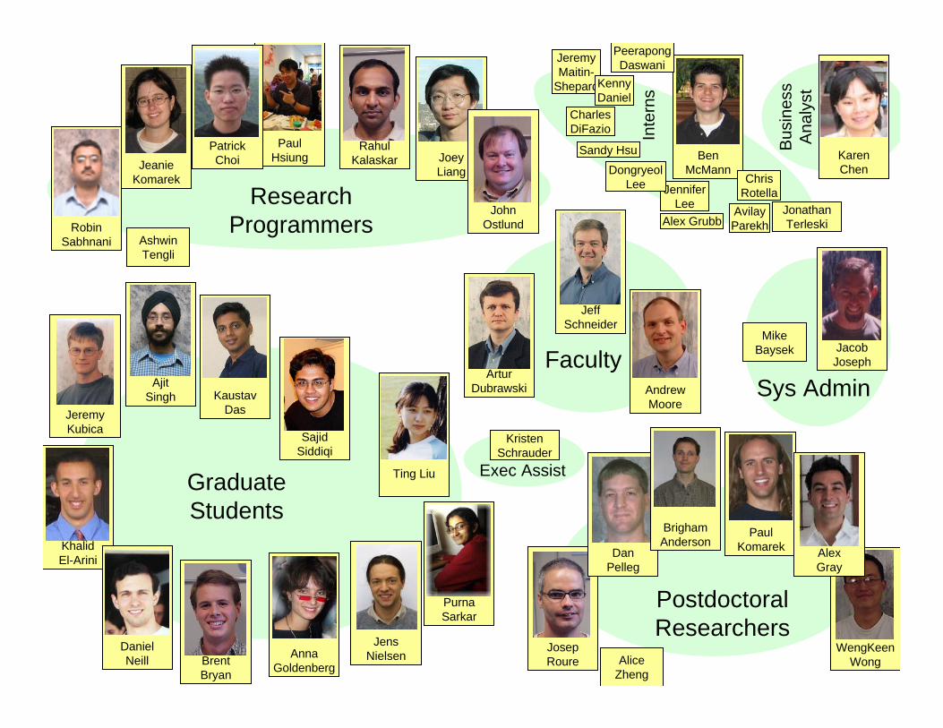
Faculty
Graduate Students
Research Programmers
Postdoctoral Researchers
Brigham Anderson
Alex Gray
Ashwin Tengli
John Ostlund
Mike Baysek
Sys Admin
Bus
ines
s A
naly
st
Inte
rns
PeerapongDaswani
Alex Grubb
Jeremy Maitin-
Shepard
Jonathan Terleski
Chris Rotella
AvilayParekh
Jennifer Lee
DongryeolLee
Sandy Hsu
Charles DiFazio
Kenny Daniel
Kristen Schrauder
Exec Assist
Alice Zheng
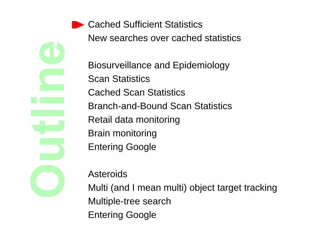
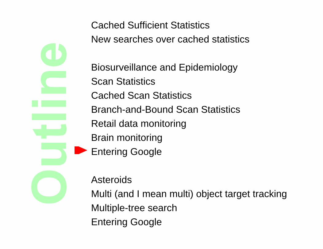
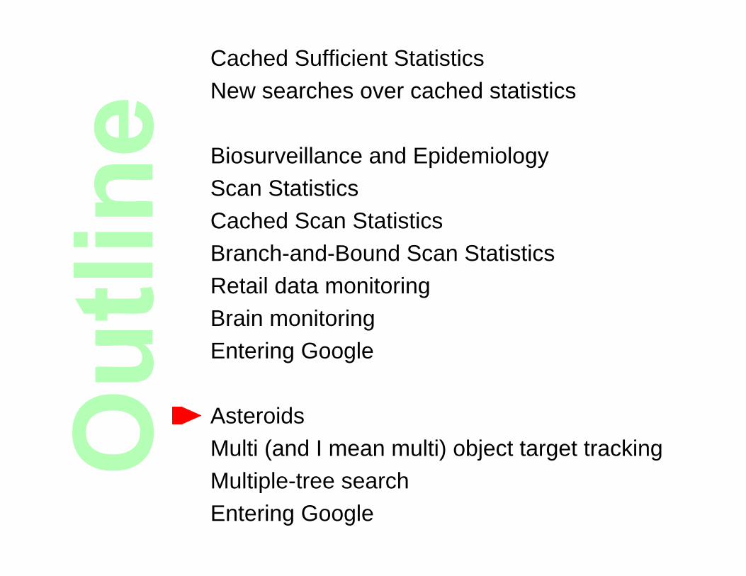
Cached Sufficient StatisticsNew searches over cached statistics
Biosurveillance and EpidemiologyScan StatisticsCached Scan StatisticsBranch-and-Bound Scan StatisticsRetail data monitoringBrain monitoringEntering Google
AsteroidsMulti (and I mean multi) object target tracking Multiple-tree searchEntering Google
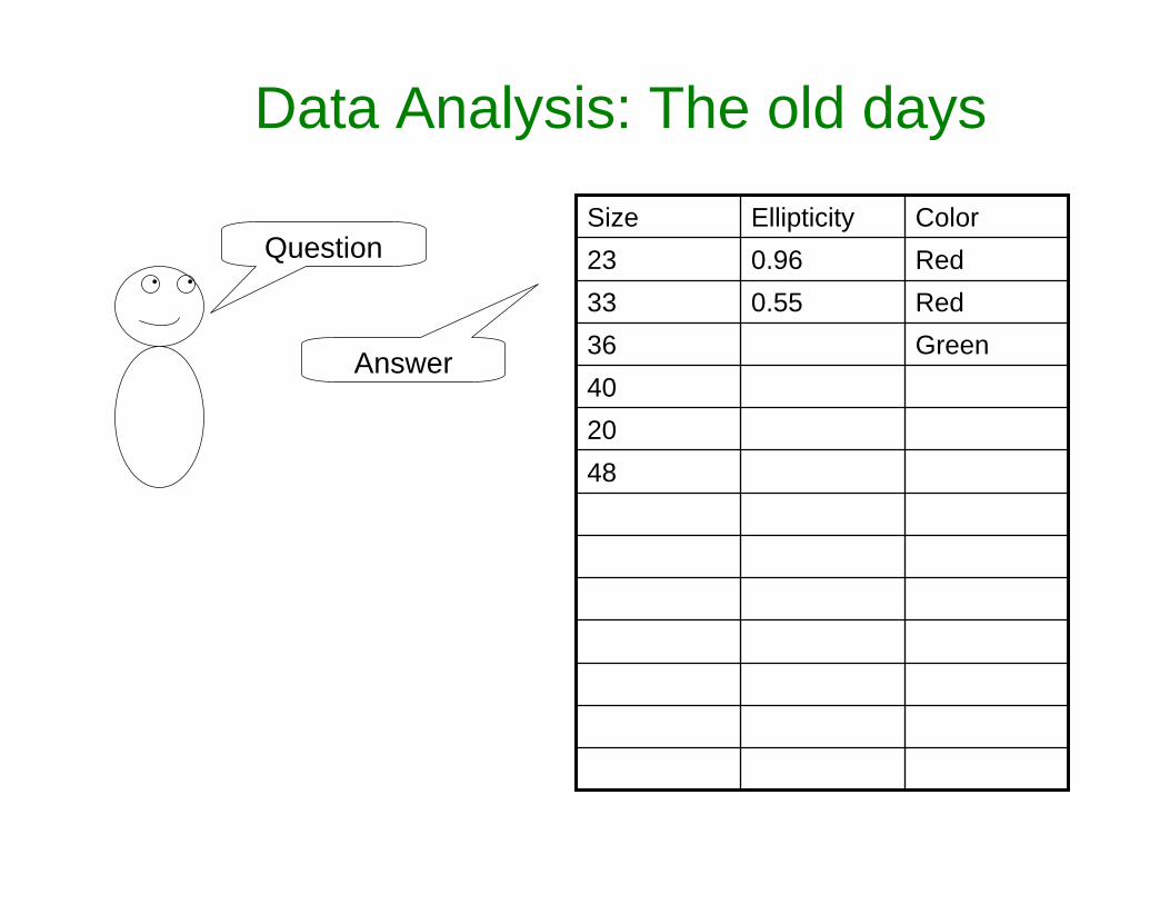
Data Analysis: The old days
• •
Question
482040
Green36Red0.5533Red0.9623ColorEllipticitySize
Answer
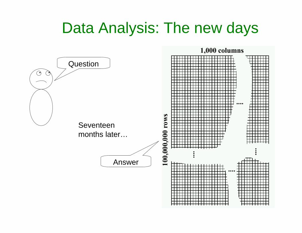
Data Analysis: The new days
• •
Question
Answer
Seventeen months later…
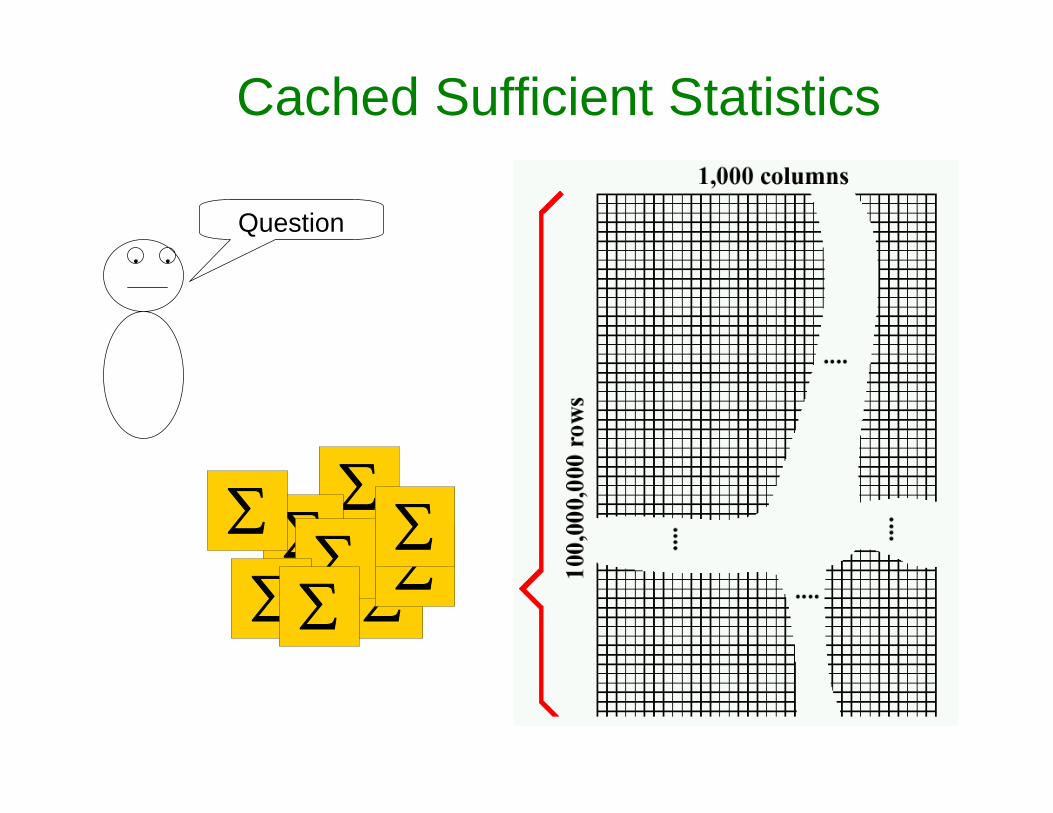
Cached Sufficient Statistics
• •
Question
∑∑
∑∑
∑ ∑∑
∑ ∑
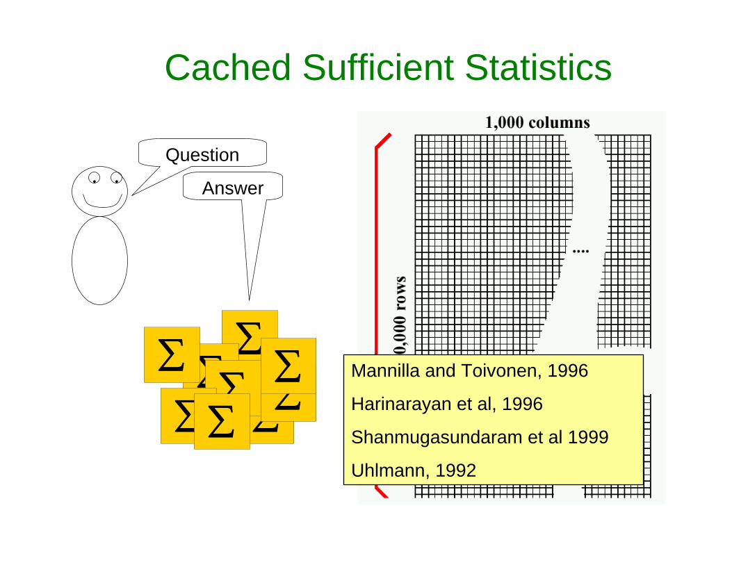
Cached Sufficient Statistics
• •
Question
∑∑
∑∑
∑ ∑∑
∑ ∑
Answer
Mannilla and Toivonen, 1996
Harinarayan et al, 1996
Shanmugasundaram et al 1999
Uhlmann, 1992
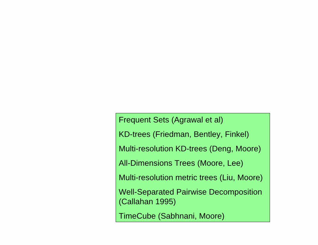
Frequent Sets (Agrawal et al)
KD-trees (Friedman, Bentley, Finkel)
Multi-resolution KD-trees (Deng, Moore)
All-Dimensions Trees (Moore, Lee)
Multi-resolution metric trees (Liu, Moore)
Well-Separated Pairwise Decomposition (Callahan 1995)
TimeCube (Sabhnani, Moore)
Cached Sufficient StatisticsNew searches over cached statistics
Biosurveillance and EpidemiologyScan StatisticsCached Scan StatisticsBranch-and-Bound Scan StatisticsRetail data monitoringBrain monitoringEntering Google
AsteroidsMulti (and I mean multi) object target tracking Multiple-tree searchEntering Google
Roberto BayardoGeoff WebbMartin KulldorfPregibon and DuMouchel
Cached Sufficient StatisticsNew searches over cached statistics
Biosurveillance and EpidemiologyScan StatisticsCached Scan StatisticsBranch-and-Bound Scan StatisticsRetail data monitoringBrain monitoringEntering Google
AsteroidsMulti (and I mean multi) object target tracking Multiple-tree searchEntering Google
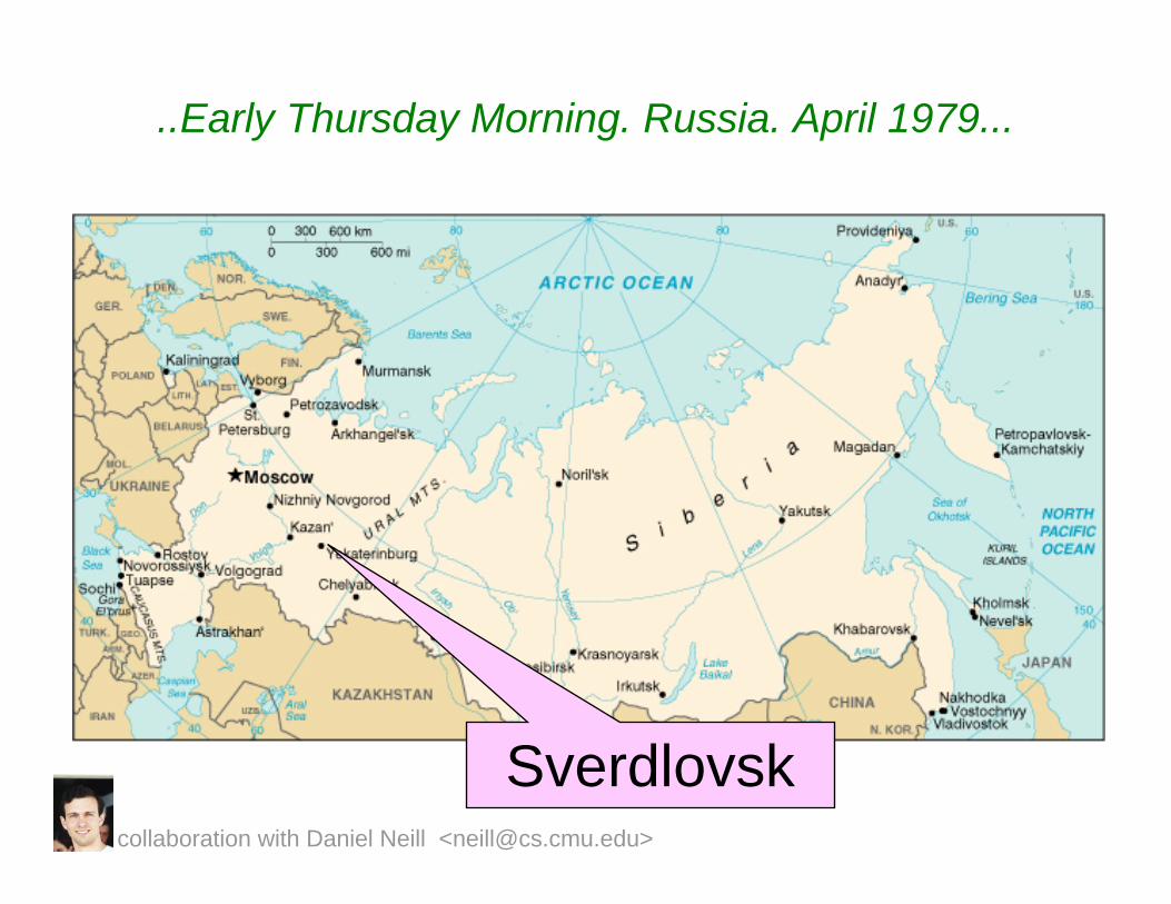
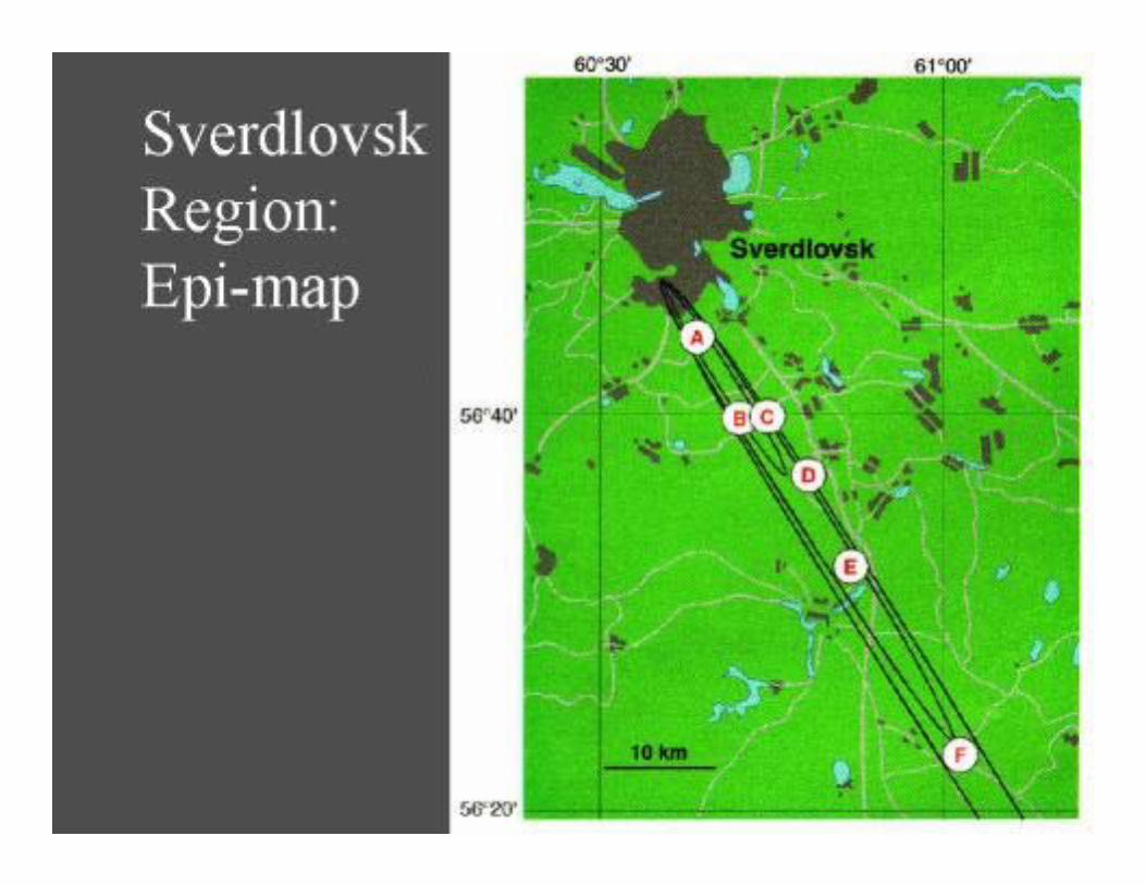
..Early Thursday Morning. Russia. April 1979...
Sverdlovskcollaboration with Daniel Neill <[email protected]>

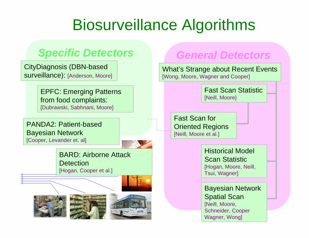
Biosurveillance Algorithms
General Detectors
PANDA2: Patient-based Bayesian Network[Cooper, Levander et. al]
BARD: Airborne Attack Detection[Hogan, Cooper et al.]
Fast Scan Statistic[Neill, Moore]
Fast Scan for Oriented Regions[Neill, Moore et al.]
Historical Model Scan Statistic[Hogan, Moore, Neill, Tsui, Wagner]
Bayesian Network Spatial Scan[Neill, Moore, Schneider, Cooper Wagner, Wong]
Specific DetectorsWhat’s Strange about Recent Events [Wong, Moore, Wagner and Cooper]
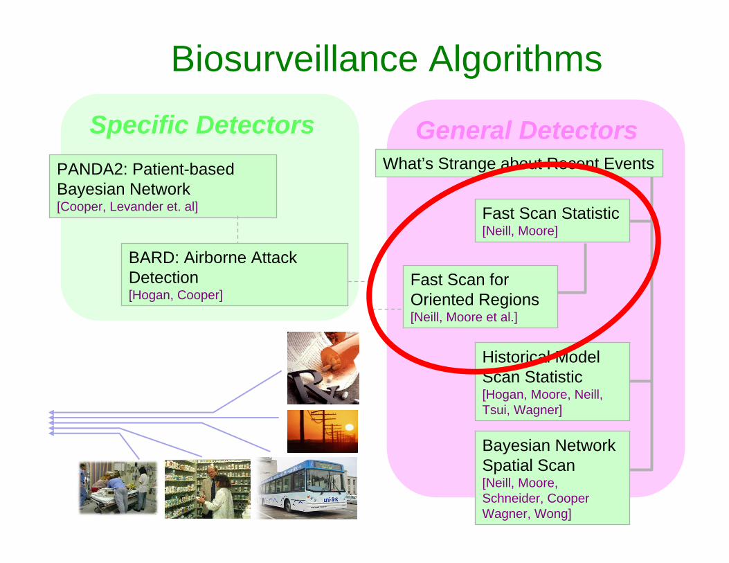
Biosurveillance Algorithms
CityDiagnosis (DBN-based surveillance): [Anderson, Moore]
EPFC: Emerging Patterns from food complaints: [Dubrawski, Sabhnani, Moore]
General DetectorsPANDA2: Patient-based Bayesian Network[Cooper, Levander et. al]
BARD: Airborne Attack Detection[Hogan, Cooper]
Fast Scan Statistic[Neill, Moore]
Fast Scan for Oriented Regions[Neill, Moore et al.]
Historical Model Scan Statistic[Hogan, Moore, Neill, Tsui, Wagner]
Bayesian Network Spatial Scan[Neill, Moore, Schneider, Cooper Wagner, Wong]
Specific DetectorsWhat’s Strange about Recent Events
Biosurveillance Algorithms
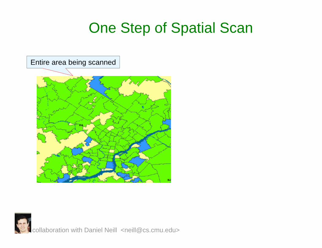
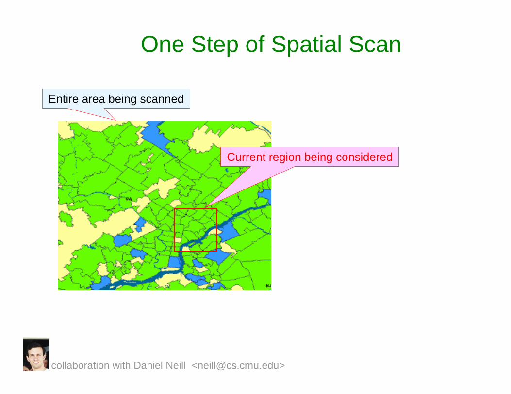
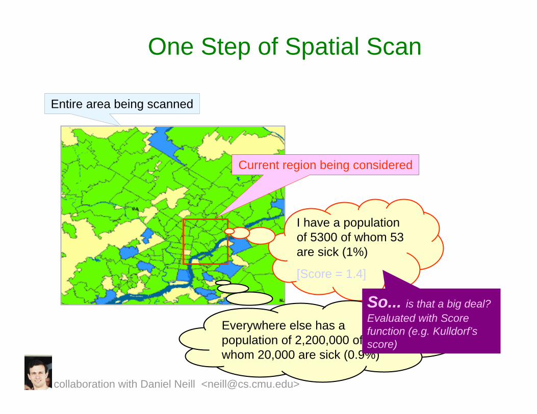
One Step of Spatial Scan
Entire area being scanned
collaboration with Daniel Neill <[email protected]>
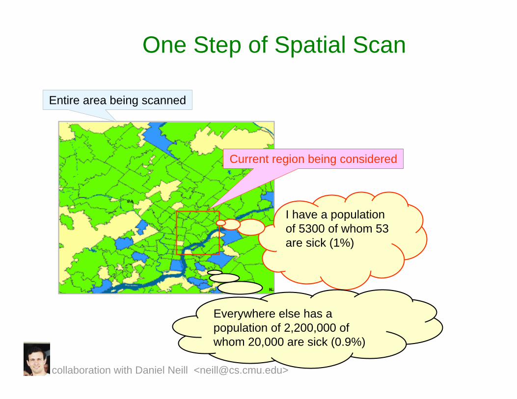
One Step of Spatial Scan
Entire area being scanned
Current region being considered
collaboration with Daniel Neill <[email protected]>
One Step of Spatial Scan
Entire area being scanned
Current region being considered
I have a population of 5300 of whom 53 are sick (1%)
Everywhere else has a population of 2,200,000 of whom 20,000 are sick (0.9%)
collaboration with Daniel Neill <[email protected]>
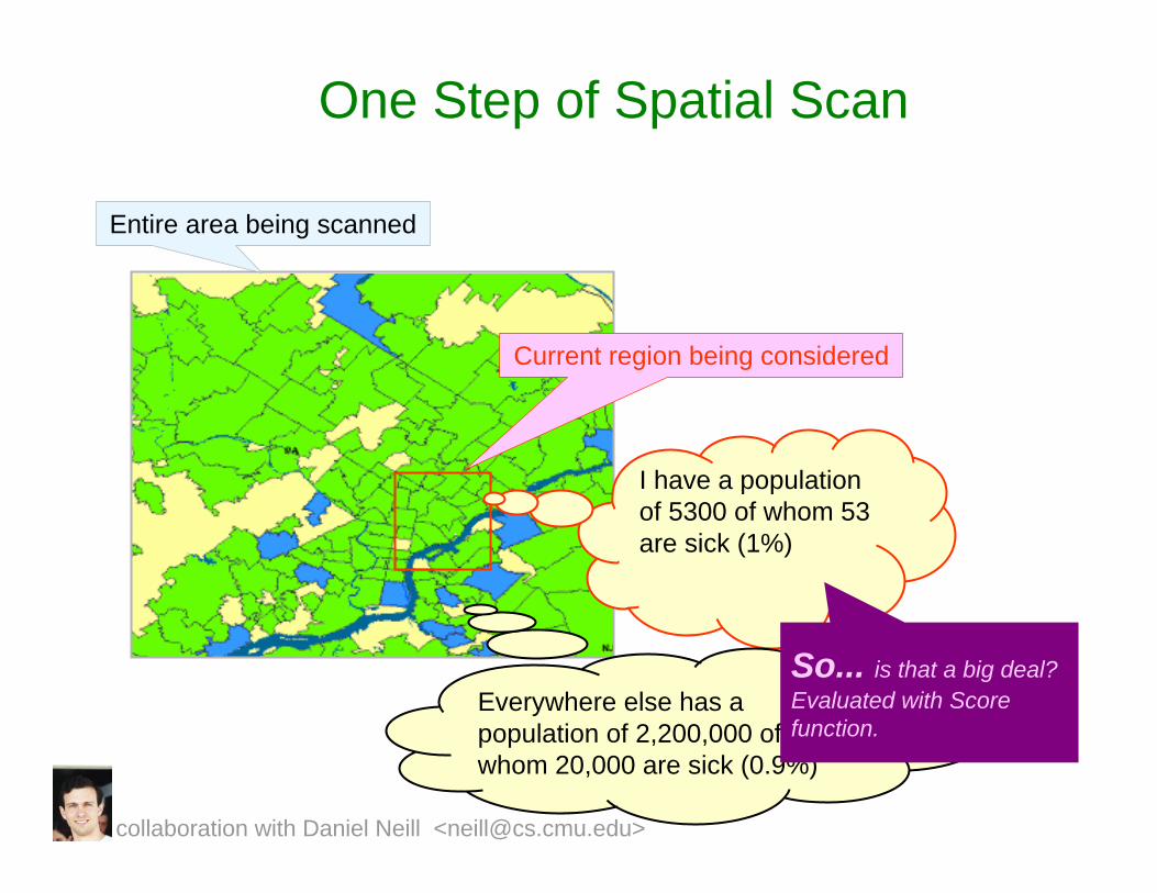
One Step of Spatial Scan
Entire area being scanned
Current region being considered
I have a population of 5300 of whom 53 are sick (1%)
Everywhere else has a population of 2,200,000 of whom 20,000 are sick (0.9%)
So... is that a big deal? Evaluated with Score function.
collaboration with Daniel Neill <[email protected]>
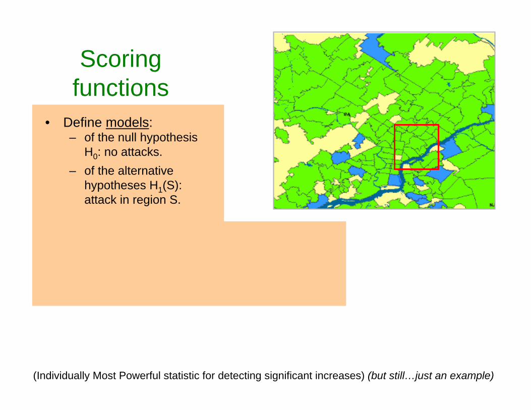
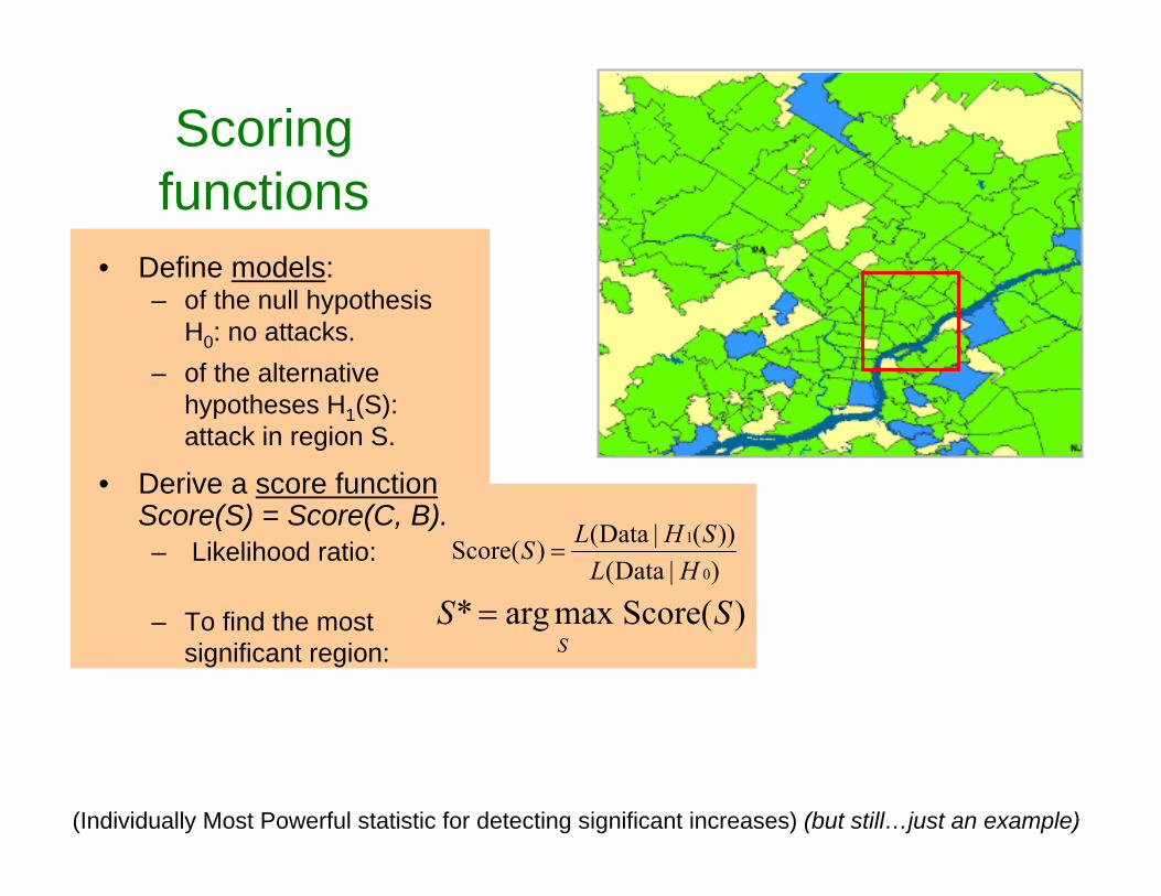
Scoring functions
• Define models:– of the null hypothesis
H0: no attacks. – of the alternative
hypotheses H1(S): attack in region S.
(Individually Most Powerful statistic for detecting significant increases) (but still…just an example)
Scoring functions
• Define models:– of the null hypothesis
H0: no attacks. – of the alternative
hypotheses H1(S): attack in region S.
• Derive a score functionScore(S) = Score(C, B).– Likelihood ratio:
– To find the most significant region:
)| Data())(| Data()(Score
0
1
HLSHLS =
)(Scoremaxarg* SSS
=
(Individually Most Powerful statistic for detecting significant increases) (but still…just an example)
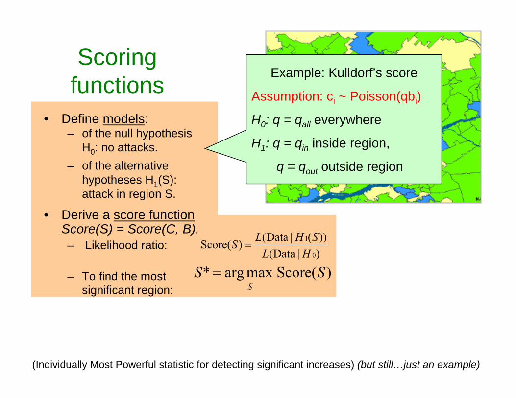
Scoring functions
• Define models:– of the null hypothesis
H0: no attacks. – of the alternative
hypotheses H1(S): attack in region S.
• Derive a score functionScore(S) = Score(C, B).– Likelihood ratio:
– To find the most significant region:
)| Data())(| Data()(Score
0
1
HLSHLS =
)(Scoremaxarg* SSS
=
Example: Kulldorf’s score
Assumption: ci ~ Poisson(qbi)
H0: q = qall everywhere
H1: q = qin inside region,
q = qout outside region
(Individually Most Powerful statistic for detecting significant increases) (but still…just an example)
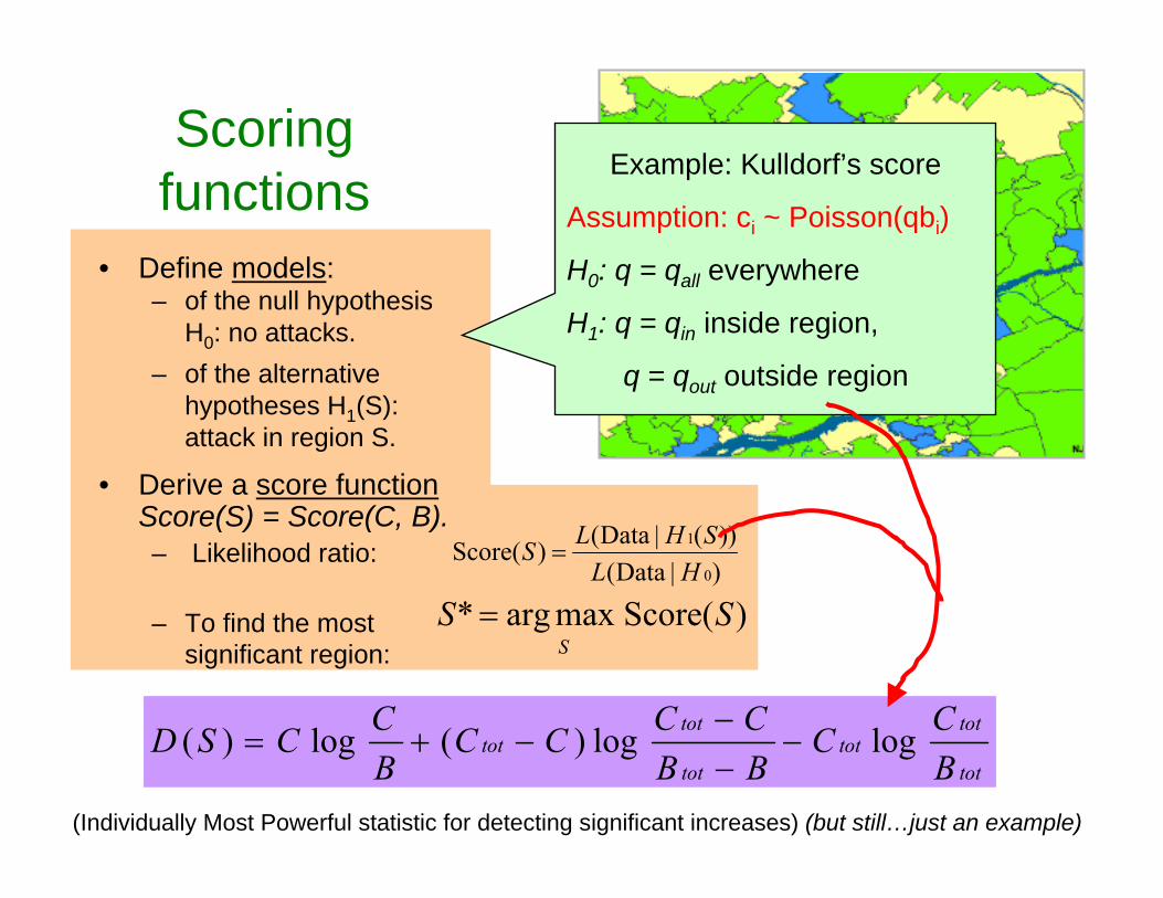
Scoring functions
• Define models:– of the null hypothesis
H0: no attacks. – of the alternative
hypotheses H1(S): attack in region S.
• Derive a score functionScore(S) = Score(C, B).– Likelihood ratio:
– To find the most significant region:
)| Data())(| Data()(Score
0
1
HLSHLS =
)(Scoremaxarg* SSS
=
Example: Kulldorf’s score
Assumption: ci ~ Poisson(qbi)
H0: q = qall everywhere
H1: q = qin inside region,
q = qout outside region
tot
tottot
tot
tottot
BCC
BBCCCC
BCCSD loglog)(log)( −
−−
−+=
(Individually Most Powerful statistic for detecting significant increases) (but still…just an example)
One Step of Spatial Scan
Entire area being scanned
Current region being considered
I have a population of 5300 of whom 53 are sick (1%)
[Score = 1.4]
Everywhere else has a population of 2,200,000 of whom 20,000 are sick (0.9%)
So... is that a big deal? Evaluated with Score function (e.g. Kulldorf’sscore)
collaboration with Daniel Neill <[email protected]>
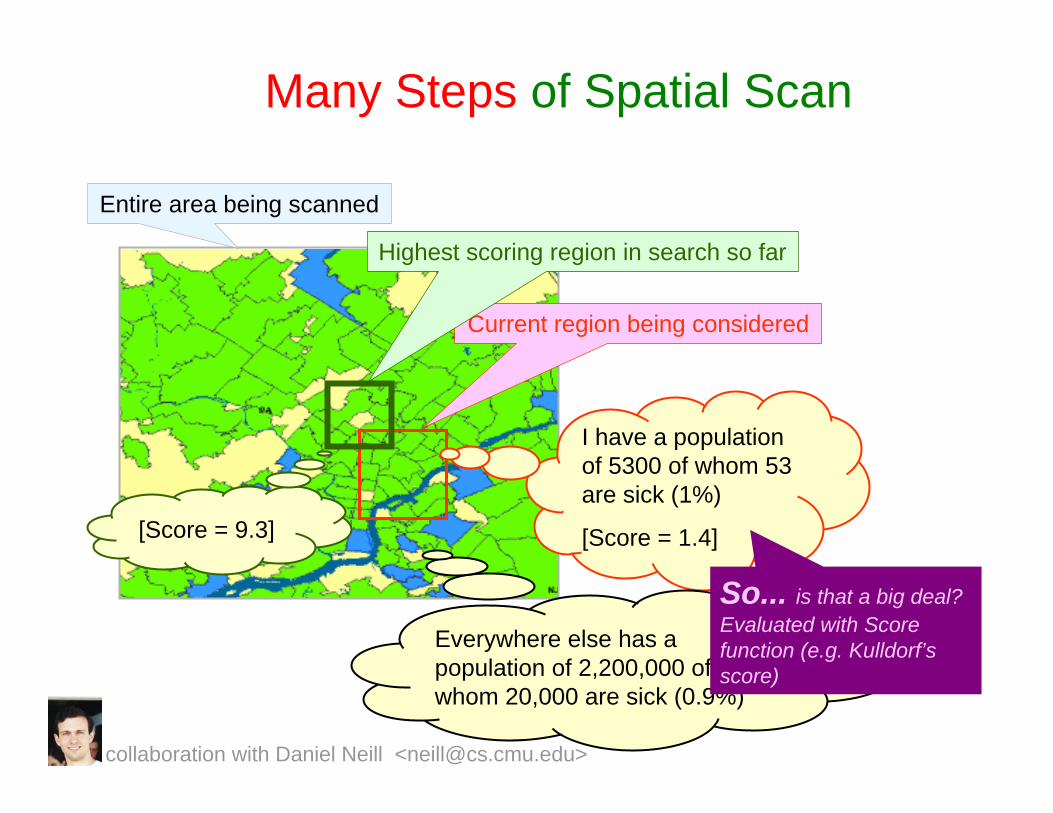
Many Steps of Spatial Scan
Entire area being scanned
Current region being considered
I have a population of 5300 of whom 53 are sick (1%)
[Score = 1.4]
Everywhere else has a population of 2,200,000 of whom 20,000 are sick (0.9%)
So... is that a big deal? Evaluated with Score function (e.g. Kulldorf’sscore)
Highest scoring region in search so far
[Score = 9.3]
collaboration with Daniel Neill <[email protected]>
collaboration with Daniel Neill <[email protected]>
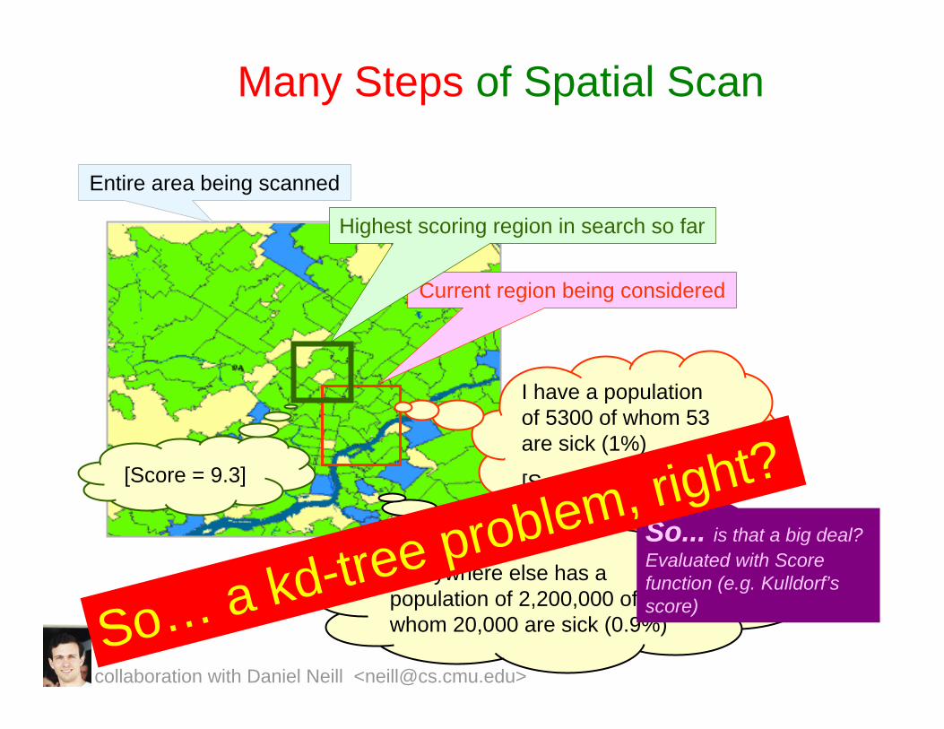
Many Steps of Spatial Scan
Entire area being scanned
Current region being considered
I have a population of 5300 of whom 53 are sick (1%)
[Score = 1.4]
Everywhere else has a population of 2,200,000 of whom 20,000 are sick (0.9%)
So... is that a big deal? Evaluated with Score function (e.g. Kulldorf’sscore)
Highest scoring region in search so far
[Score = 9.3]
So… a kd-tree problem, right?
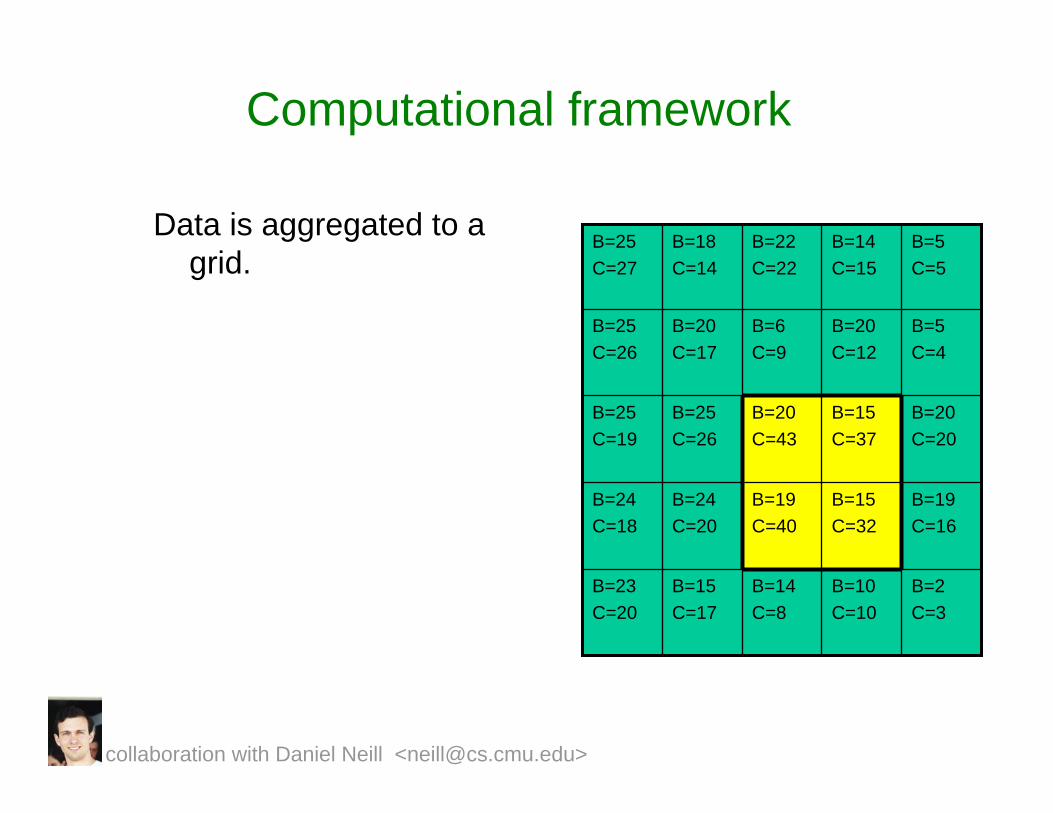
Computational framework
Data is aggregated to a grid.
B=2C=3
B=10C=10
B=14C=8
B=15C=17
B=23C=20
B=19C=16
B=15C=32
B=19C=40
B=24C=20
B=24C=18
B=20C=20
B=15C=37
B=20C=43
B=25C=26
B=25C=19
B=5C=4
B=20C=12
B=6C=9
B=20C=17
B=25C=26
B=5C=5
B=14C=15
B=22C=22
B=18C=14
B=25C=27
collaboration with Daniel Neill <[email protected]>
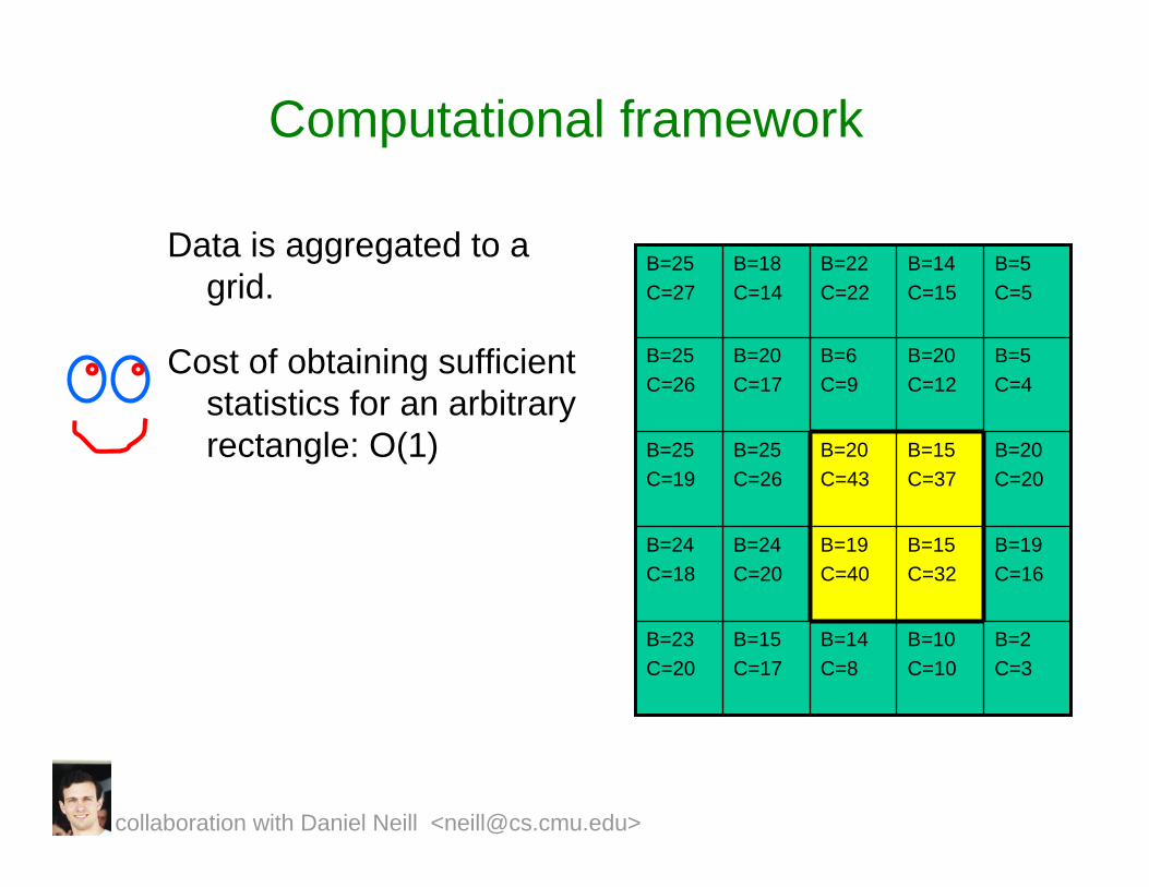
Computational framework
Data is aggregated to a grid.
Cost of obtaining sufficient statistics for an arbitrary rectangle: O(1)
B=2C=3
B=10C=10
B=14C=8
B=15C=17
B=23C=20
B=19C=16
B=15C=32
B=19C=40
B=24C=20
B=24C=18
B=20C=20
B=15C=37
B=20C=43
B=25C=26
B=25C=19
B=5C=4
B=20C=12
B=6C=9
B=20C=17
B=25C=26
B=5C=5
B=14C=15
B=22C=22
B=18C=14
B=25C=27
collaboration with Daniel Neill <[email protected]>
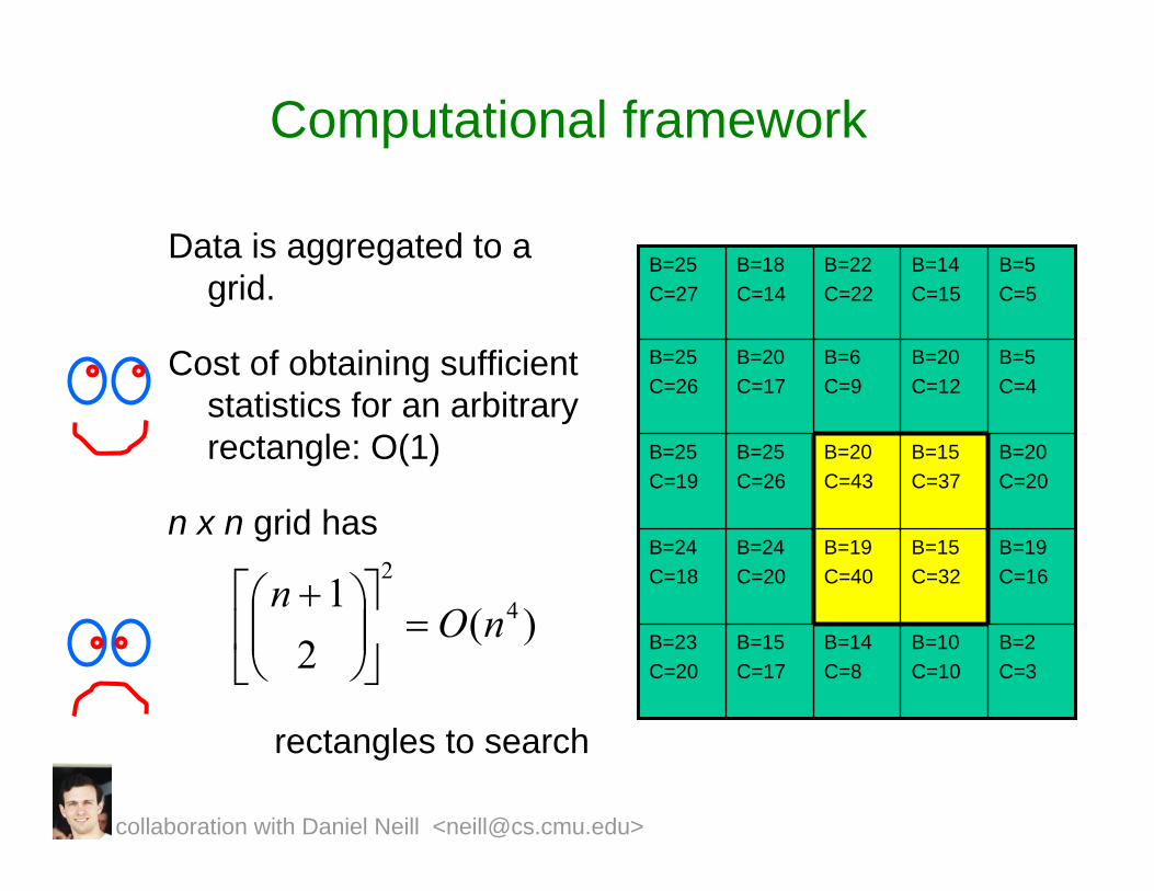
Computational framework
Data is aggregated to a grid.
Cost of obtaining sufficient statistics for an arbitrary rectangle: O(1)
n x n grid has
rectangles to search
B=2C=3
B=10C=10
B=14C=8
B=15C=17
B=23C=20
B=19C=16
B=15C=32
B=19C=40
B=24C=20
B=24C=18
B=20C=20
B=15C=37
B=20C=43
B=25C=26
B=25C=19
B=5C=4
B=20C=12
B=6C=9
B=20C=17
B=25C=26
B=5C=5
B=14C=15
B=22C=22
B=18C=14
B=25C=27
)(2
1 4
2
nOn
=⎥⎦
⎤⎢⎣
⎡⎟⎟⎠
⎞⎜⎜⎝
⎛ +
collaboration with Daniel Neill <[email protected]>

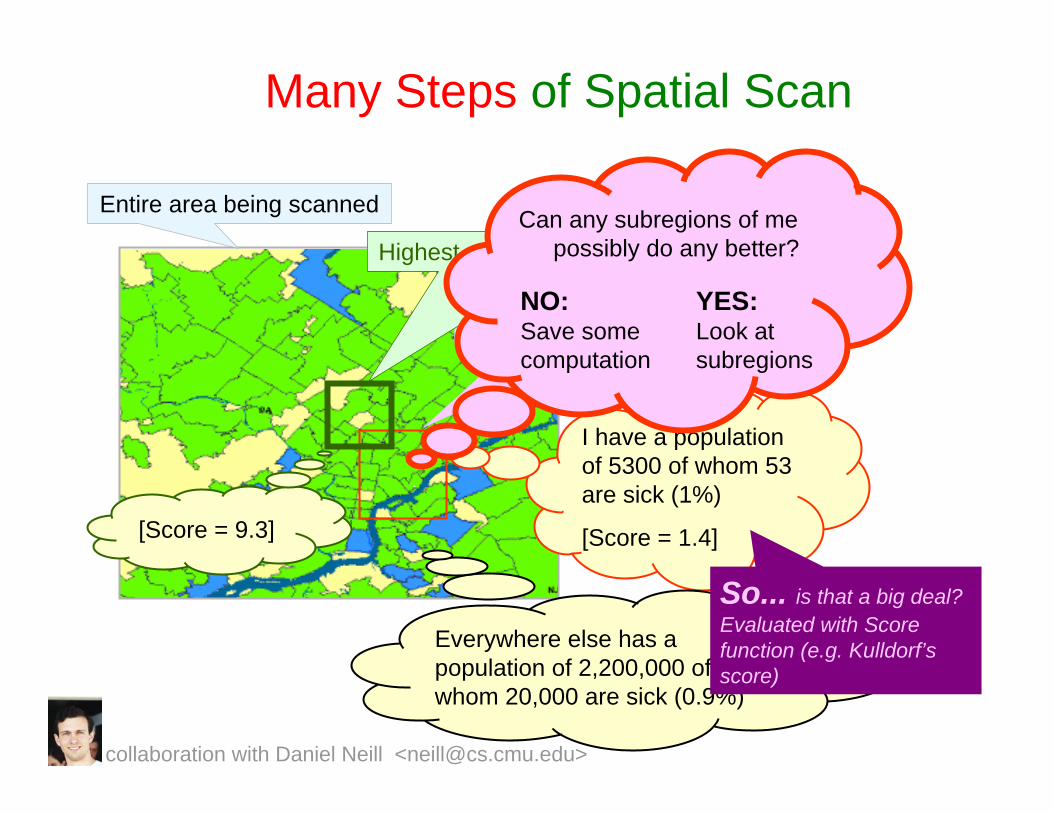
Many Steps of Spatial Scan
Entire area being scanned
Current region being considered
I have a population of 5300 of whom 53 are sick (1%)
[Score = 1.4]
Everywhere else has a population of 2,200,000 of whom 20,000 are sick (0.9%)
So... is that a big deal? Evaluated with Score function (e.g. Kulldorf’sscore)
Highest scoring region in search so far
[Score = 9.3]
collaboration with Daniel Neill <[email protected]>
Many Steps of Spatial Scan
Entire area being scanned
Current region being considered
I have a population of 5300 of whom 53 are sick (1%)
[Score = 1.4]
Everywhere else has a population of 2,200,000 of whom 20,000 are sick (0.9%)
So... is that a big deal? Evaluated with Score function (e.g. Kulldorf’sscore)
Highest scoring region in search so far
[Score = 9.3]
NO:Save some computation
Can any subregions of me possibly do any better?
YES:Look at subregions
collaboration with Daniel Neill <[email protected]>
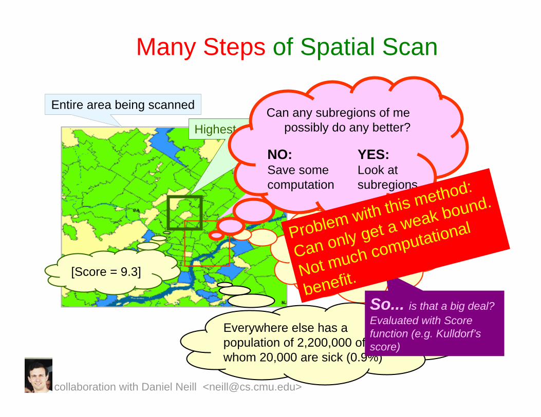
Many Steps of Spatial Scan
Entire area being scanned
Current region being considered
I have a population of 5300 of whom 53 are sick (1%) [Score = 1.4]
Everywhere else has a population of 2,200,000 of whom 20,000 are sick (0.9%)
So... is that a big deal? Evaluated with Score function (e.g. Kulldorf’sscore)
Highest scoring region in search so far
[Score = 9.3]
NO:Save some computation
Can any subregions of me possibly do any better?
YES:Look at subregions
Problem with this method:
Can only get a weak bound.
Not much computational
benefit.
collaboration with Daniel Neill <[email protected]>
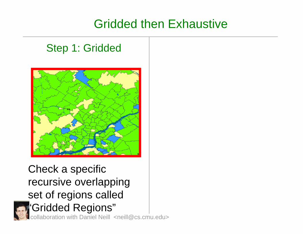
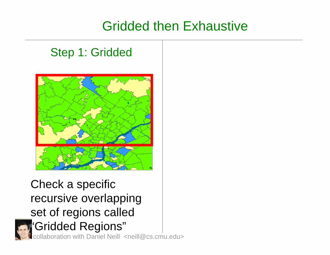
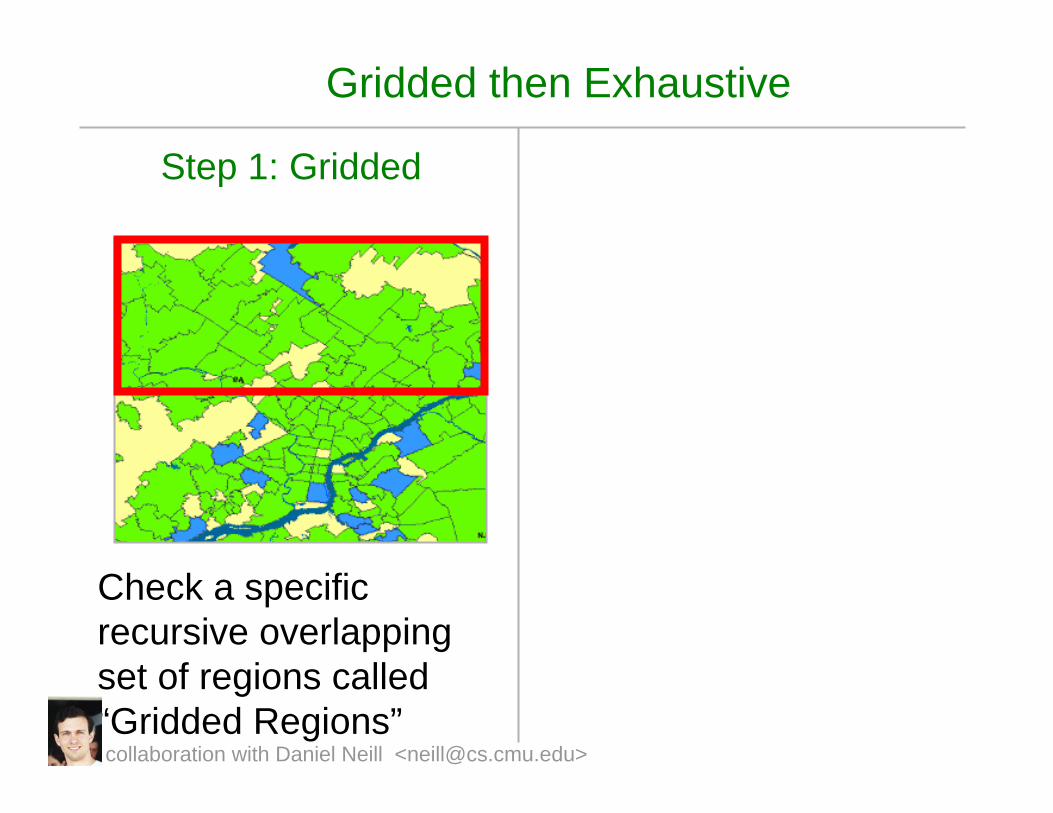
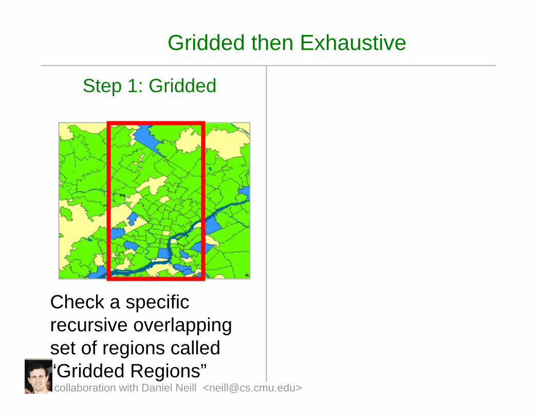
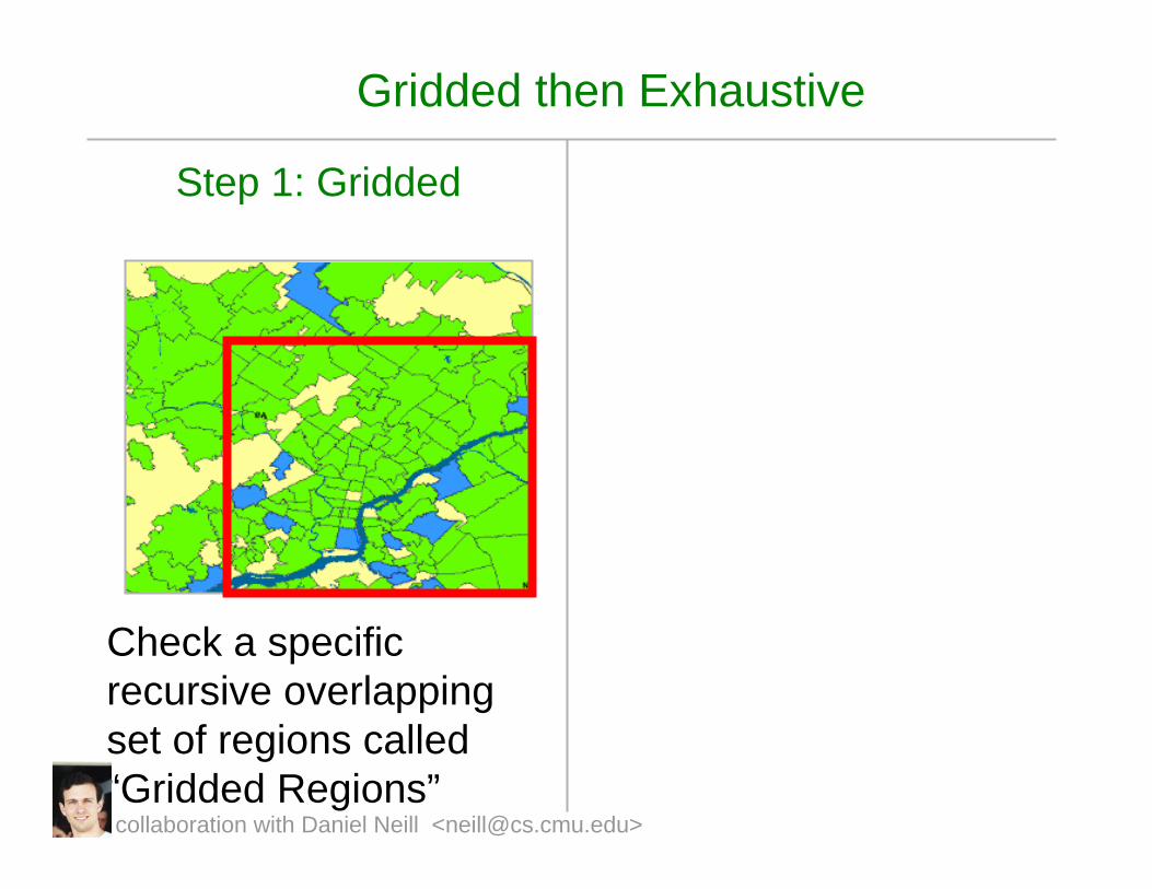
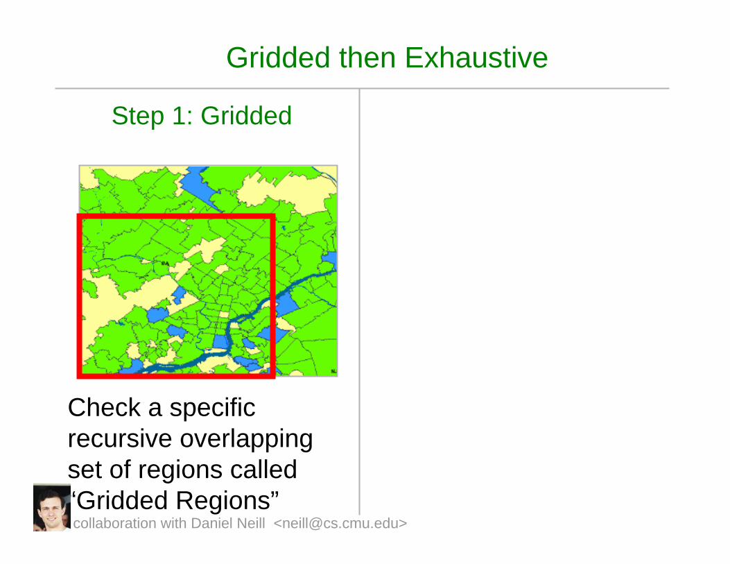
Gridded then Exhaustive
Step 1: Gridded
Check a specific recursive overlapping set of regions called “Gridded Regions”collaboration with Daniel Neill <[email protected]>
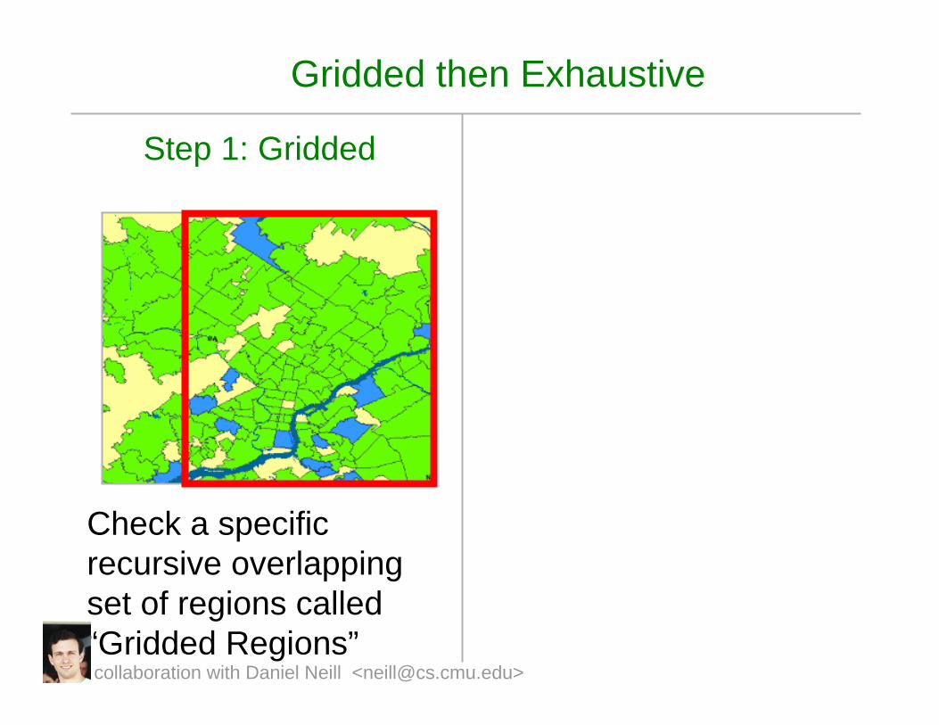
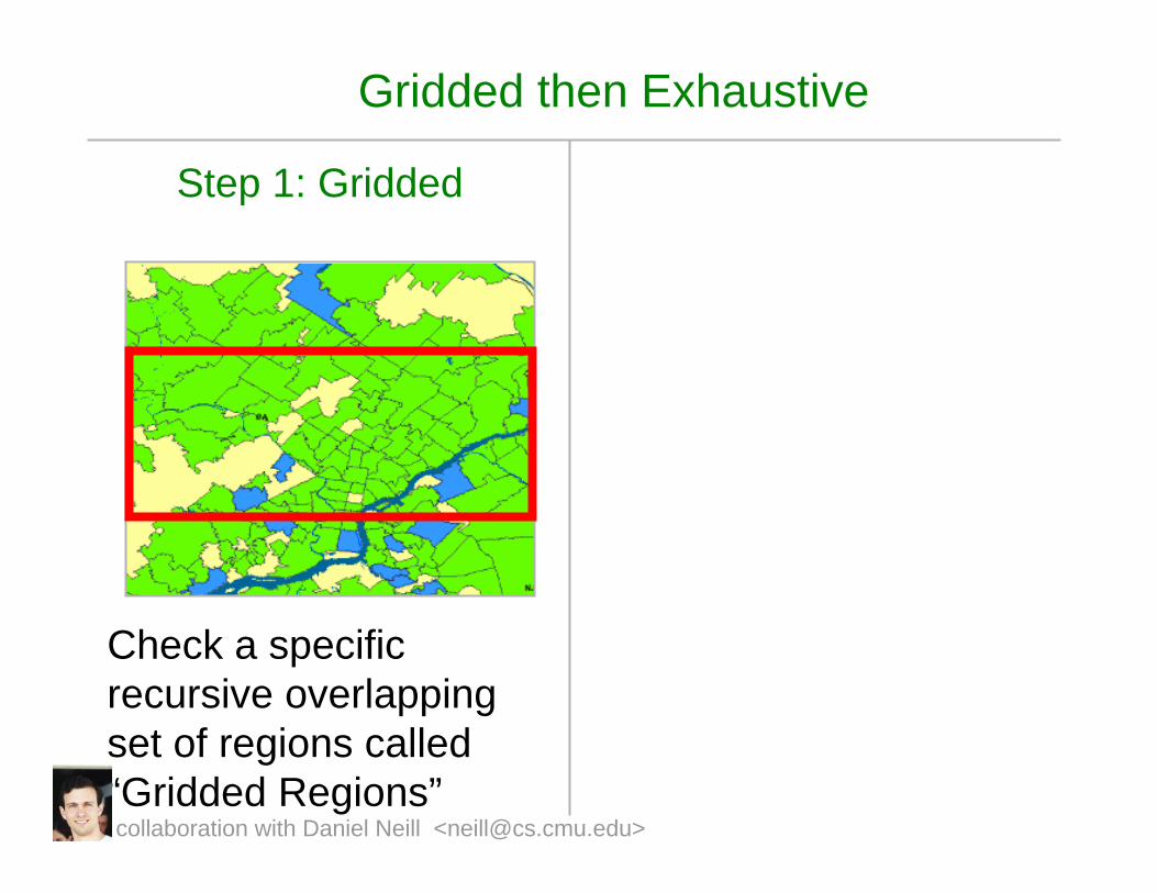
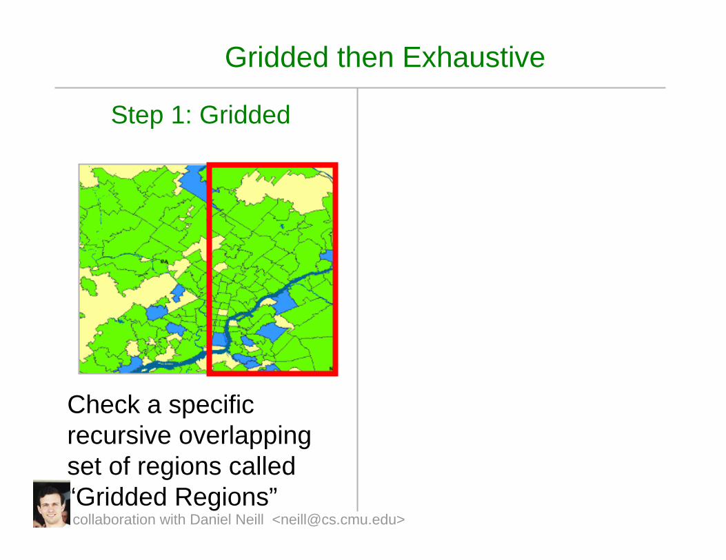
Gridded then Exhaustive
Step 1: Gridded
Check a specific recursive overlapping set of regions called “Gridded Regions”collaboration with Daniel Neill <[email protected]>
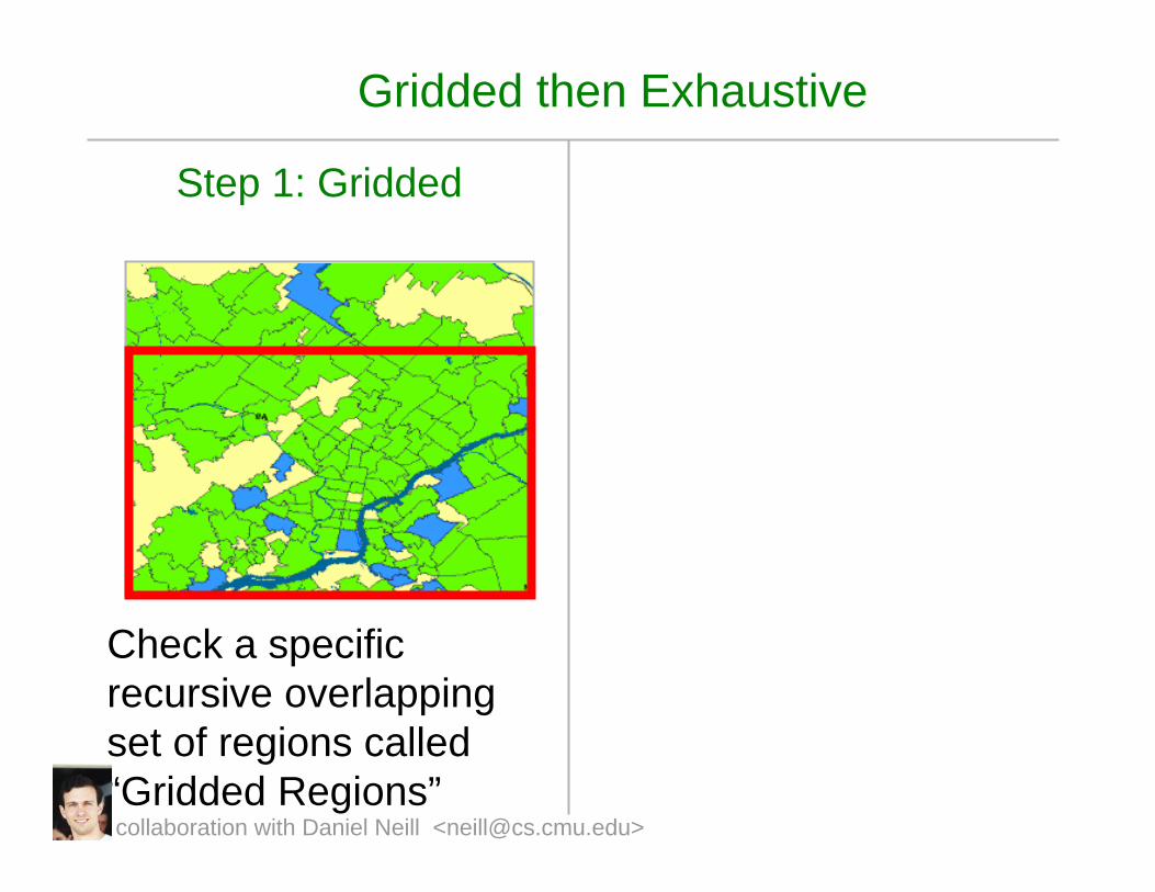
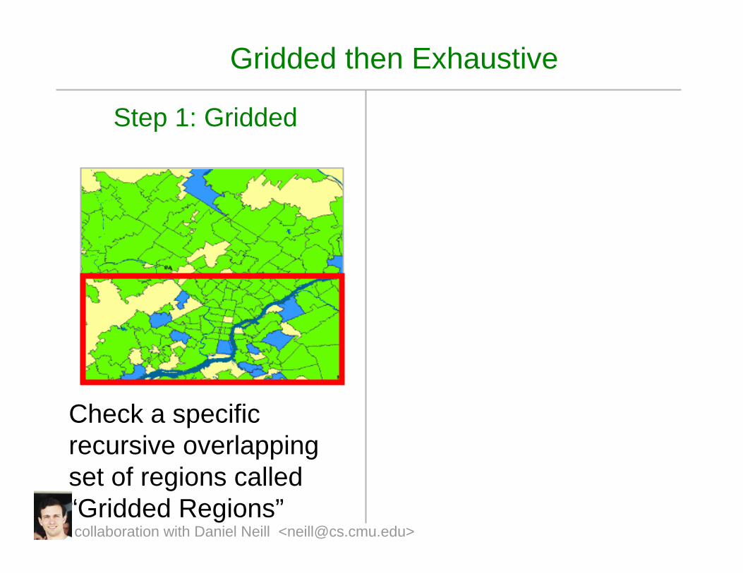
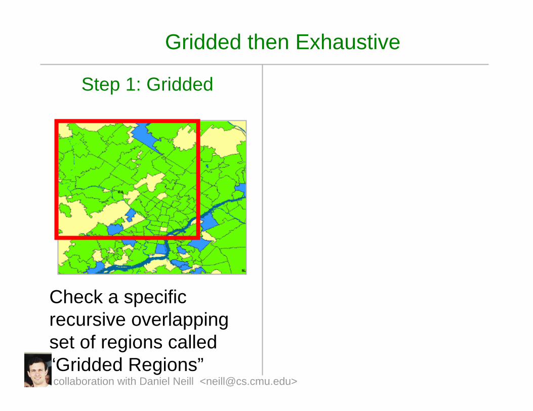
Gridded then Exhaustive
Step 1: Gridded
Check a specific recursive overlapping set of regions called “Gridded Regions”collaboration with Daniel Neill <[email protected]>
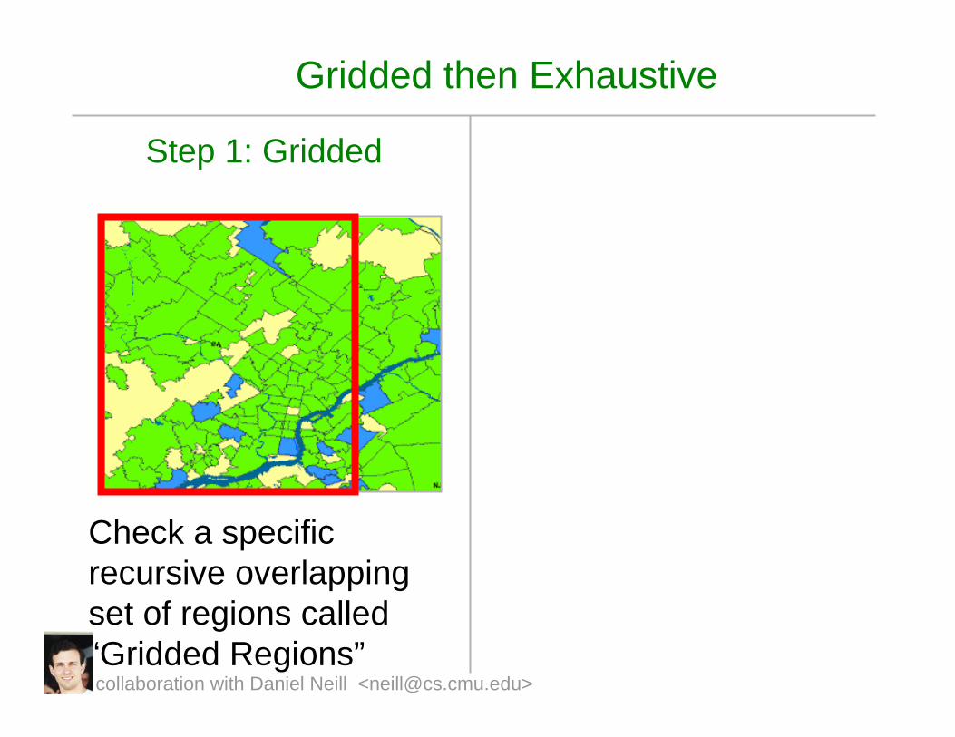
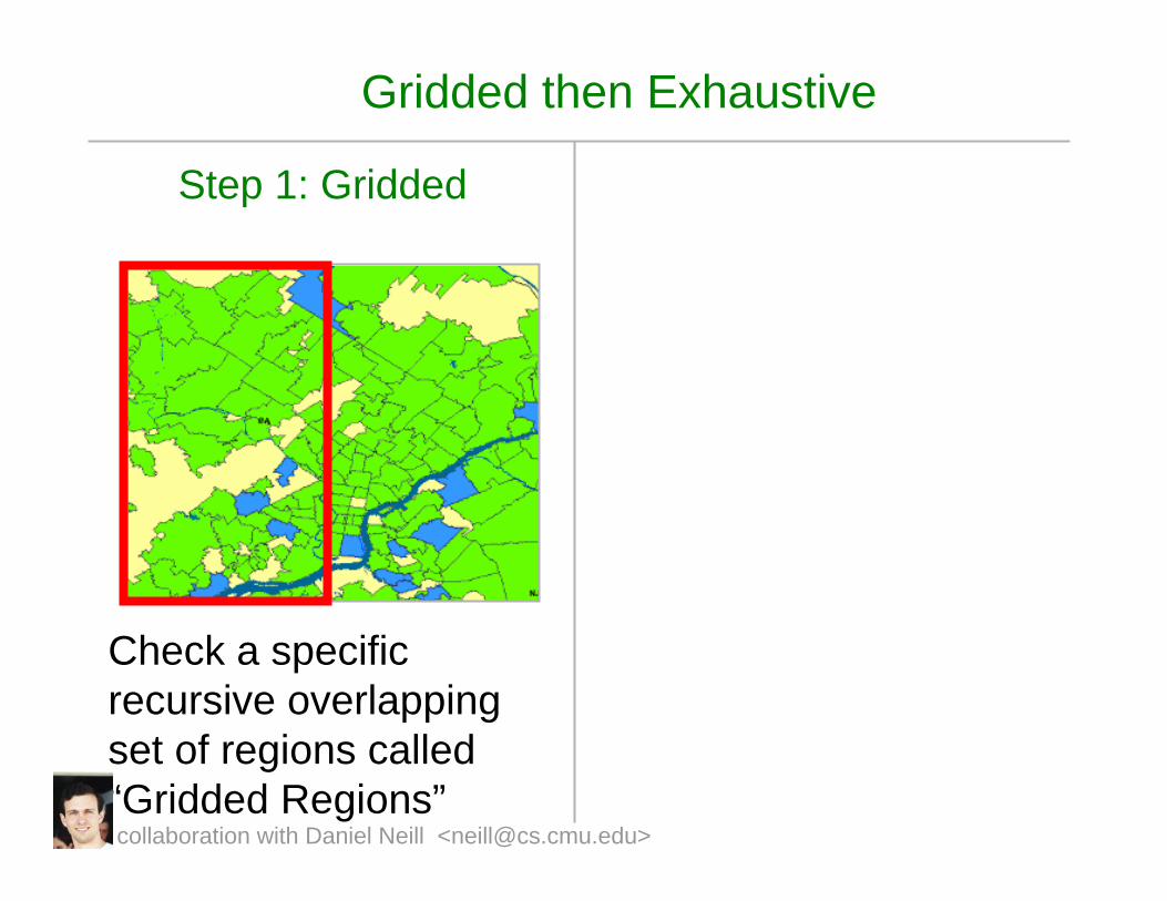
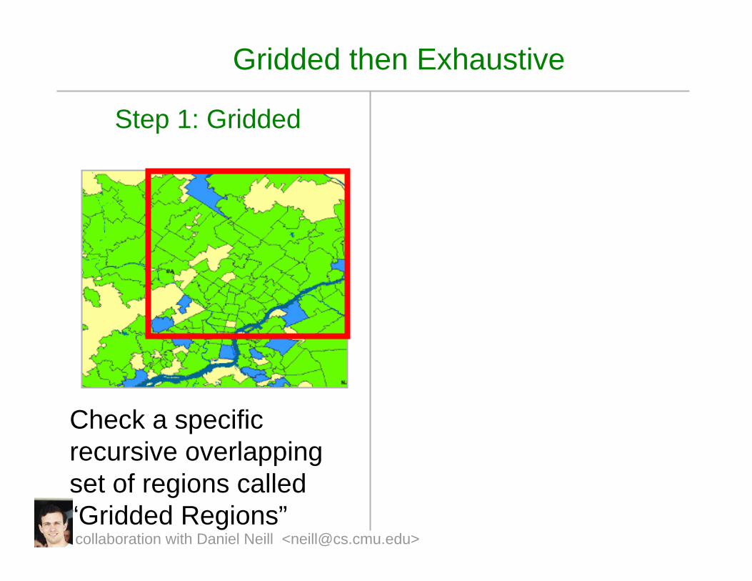
Gridded then Exhaustive
Step 1: Gridded
Check a specific recursive overlapping set of regions called “Gridded Regions”collaboration with Daniel Neill <[email protected]>
Gridded then Exhaustive
Step 1: Gridded
Check a specific recursive overlapping set of regions called “Gridded Regions”collaboration with Daniel Neill <[email protected]>
Gridded then Exhaustive
Step 1: Gridded
Check a specific recursive overlapping set of regions called “Gridded Regions”collaboration with Daniel Neill <[email protected]>
Gridded then Exhaustive
Step 1: Gridded
Check a specific recursive overlapping set of regions called “Gridded Regions”collaboration with Daniel Neill <[email protected]>
Gridded then Exhaustive
Step 1: Gridded
Check a specific recursive overlapping set of regions called “Gridded Regions”collaboration with Daniel Neill <[email protected]>
Gridded then Exhaustive
Step 1: Gridded
Check a specific recursive overlapping set of regions called “Gridded Regions”collaboration with Daniel Neill <[email protected]>
Gridded then Exhaustive
Step 1: Gridded
Check a specific recursive overlapping set of regions called “Gridded Regions”collaboration with Daniel Neill <[email protected]>
Gridded then Exhaustive
Step 1: Gridded
Check a specific recursive overlapping set of regions called “Gridded Regions”collaboration with Daniel Neill <[email protected]>
Gridded then Exhaustive
Step 1: Gridded
Check a specific recursive overlapping set of regions called “Gridded Regions”collaboration with Daniel Neill <[email protected]>
Gridded then Exhaustive
Step 1: Gridded
Check a specific recursive overlapping set of regions called “Gridded Regions”collaboration with Daniel Neill <[email protected]>
Gridded then Exhaustive
Step 1: Gridded
Check a specific recursive overlapping set of regions called “Gridded Regions”collaboration with Daniel Neill <[email protected]>
Gridded then Exhaustive
Step 1: Gridded
Check a specific recursive overlapping set of regions called “Gridded Regions”collaboration with Daniel Neill <[email protected]>
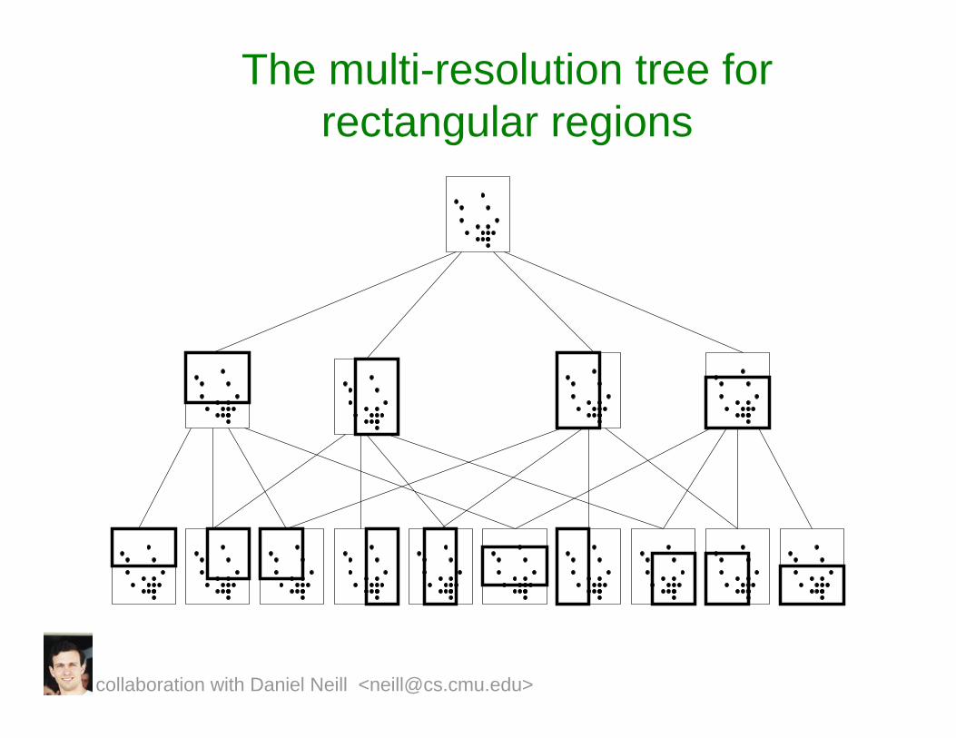
The multi-resolution tree for rectangular regions
collaboration with Daniel Neill <[email protected]>
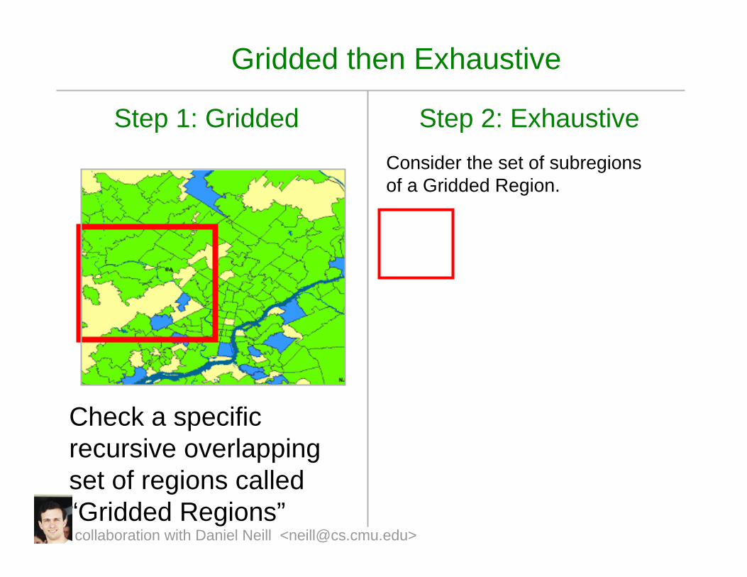
Gridded then Exhaustive
Step 1: Gridded
Check a specific recursive overlapping set of regions called “Gridded Regions”
Step 2: ExhaustiveConsider the set of subregionsof a Gridded Region.
collaboration with Daniel Neill <[email protected]>
collaboration with Daniel Neill <[email protected]>
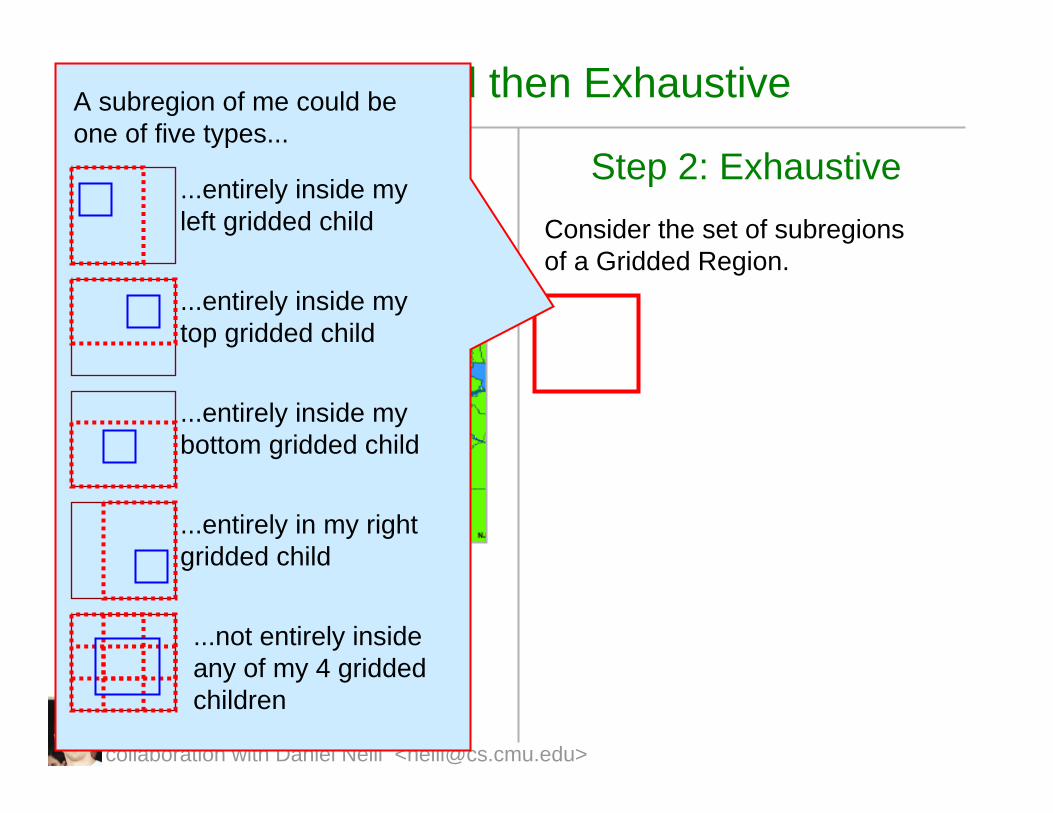
Gridded then Exhaustive
Step 1: Gridded
Check a specific recursive overlapping set of regions called “Gridded Regions”
Step 2: ExhaustiveConsider the set of subregionsof a Gridded Region.
A subregion of me could be one of five types...
...entirely inside my left gridded child
...not entirely inside any of my 4 griddedchildren
...entirely in my right gridded child
...entirely inside my bottom gridded child
...entirely inside my top gridded child
collaboration with Daniel Neill <[email protected]>
Gridded then Exhaustive
Step 1: Gridded
Check a specific recursive overlapping set of regions called “Gridded Regions”
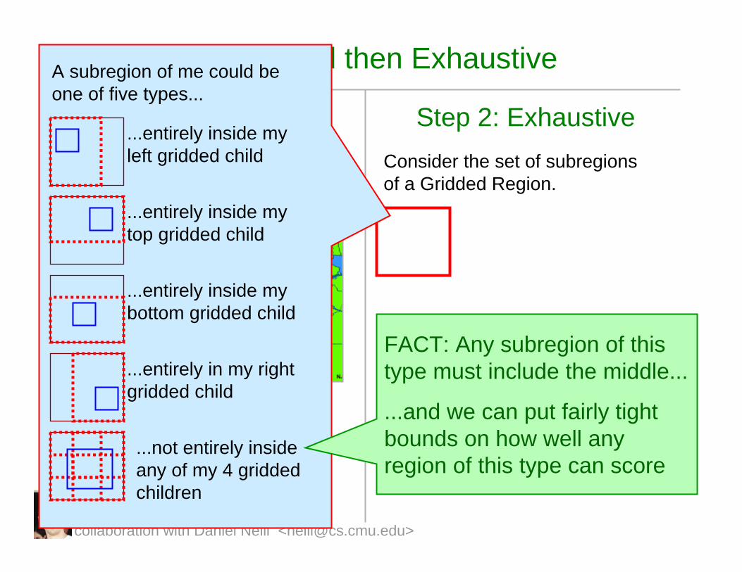
Step 2: ExhaustiveConsider the set of subregionsof a Gridded Region.
A subregion of me could be one of five types...
...entirely inside my left gridded child
...not entirely inside any of my 4 griddedchildren
...entirely in my right gridded child
...entirely inside my bottom gridded child
...entirely inside my top gridded child
FACT: Any subregion of this type must include the middle...
...and we can put fairly tight bounds on how well any region of this type can score
collaboration with Daniel Neill <[email protected]>
Gridded then Exhaustive
Step 1: Gridded
Check a specific recursive overlapping set of regions called “Gridded Regions”
Step 2: ExhaustiveConsider the set of subregionsof a Gridded Region.
A subregion of me could be one of five types...
...entirely inside my left gridded child
...not entirely inside any of my 4 griddedchildren
...entirely in my right gridded child
...entirely inside my bottom gridded child
...entirely inside my top gridded child
FACT: Any subregion of this type must include the middle...
...and we can put fairly tight bounds on how well any region of this type can score
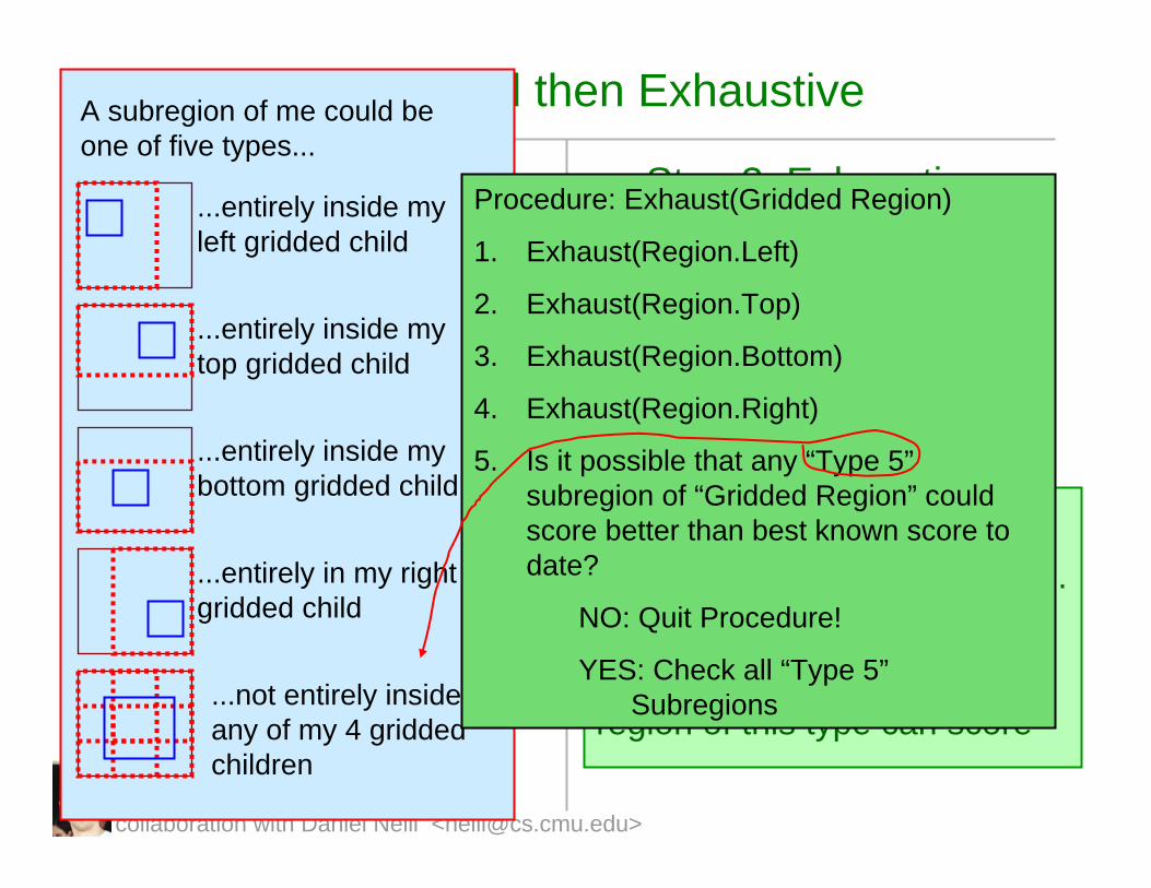
Procedure: Exhaust(Gridded Region)
1. Exhaust(Region.Left)
2. Exhaust(Region.Top)
3. Exhaust(Region.Bottom)
4. Exhaust(Region.Right)
5. Is it possible that any “Type 5”subregion of “Gridded Region” could score better than best known score to date?
NO: Quit Procedure!
YES: Check all “Type 5”Subregions
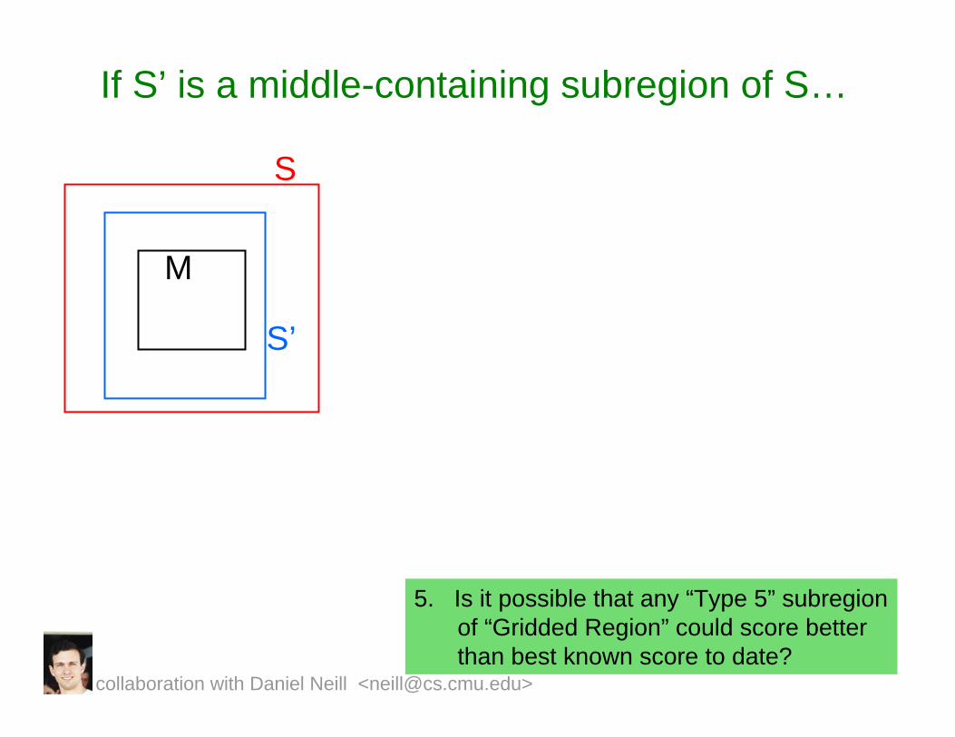
If S’ is a middle-containing subregion of S…
5. Is it possible that any “Type 5” subregionof “Gridded Region” could score better than best known score to date?
S
M
S’
collaboration with Daniel Neill <[email protected]>
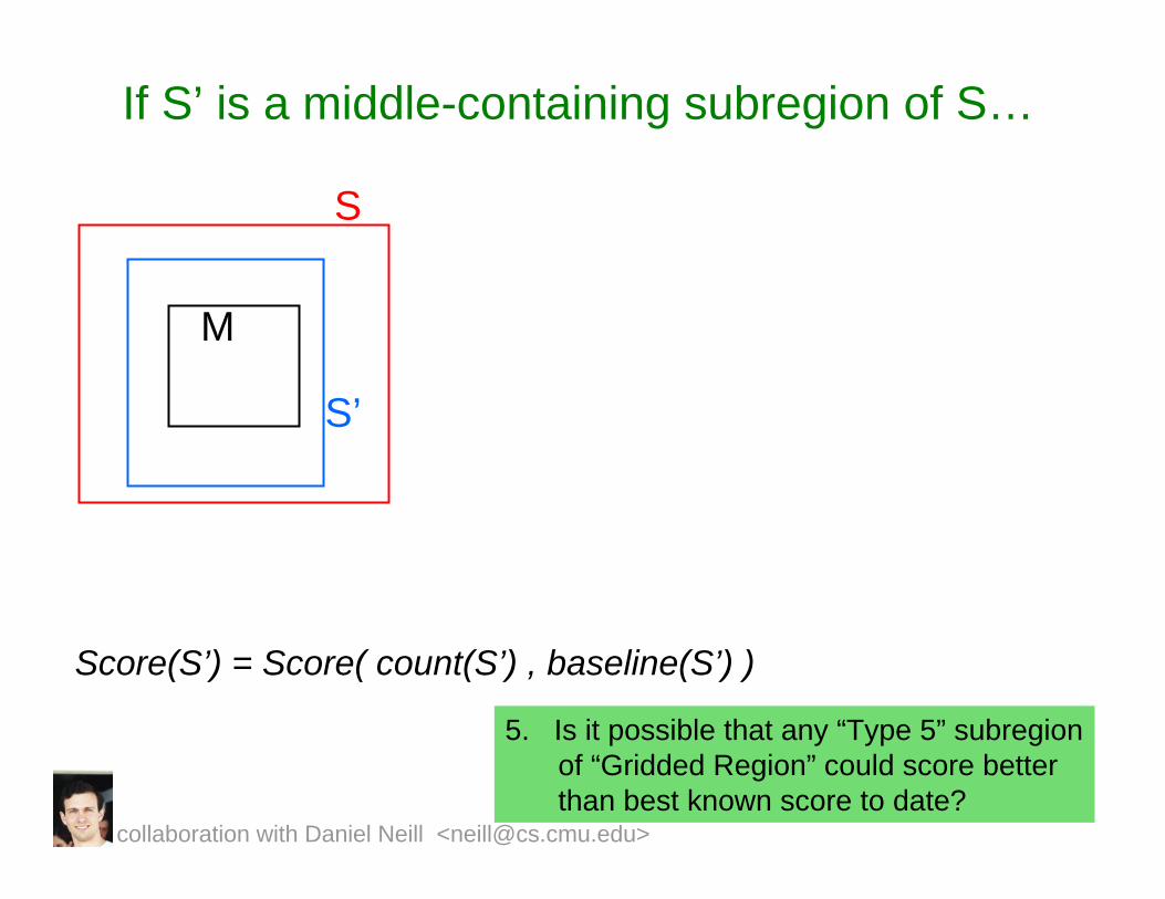
If S’ is a middle-containing subregion of S…
5. Is it possible that any “Type 5” subregionof “Gridded Region” could score better than best known score to date?
S
M
S’
Score(S’) = Score( count(S’) , baseline(S’) )
collaboration with Daniel Neill <[email protected]>

If S’ is a middle-containing subregion of S…
5. Is it possible that any “Type 5” subregionof “Gridded Region” could score better than best known score to date?
S
M
S’
)()'()()'(
MbSbMcScdinc −
−≥
)()'()( SbSbMb ≤≤
)()'()( ScScMc ≤≤
)'()'(
max SbScd ≥
)'()()'()(
min SbSbScScd
−−
≤
Score(S’) = Score( count(S’) , baseline(S’) )
An upper bound of c/b for any subregionof S-M
An upper bound of c/b for any subregionof S that contains M
A lower bound on c/bfor any subregion of S that excludes M
collaboration with Daniel Neill <[email protected]>
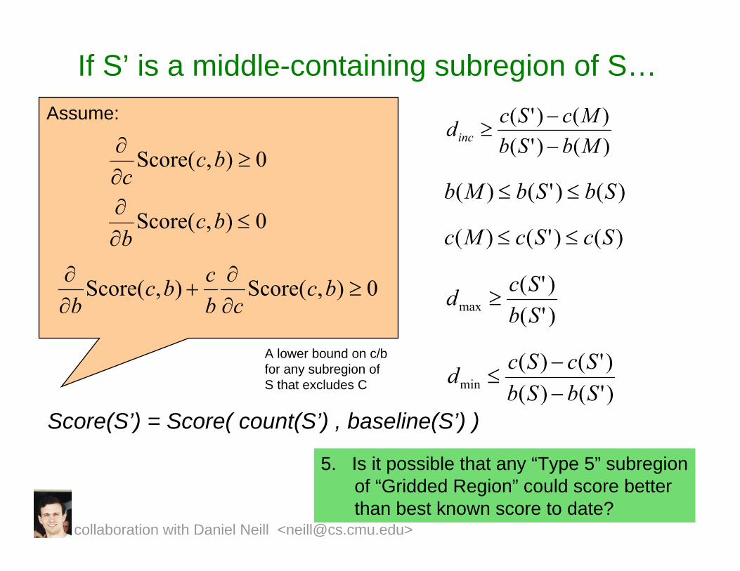
If S’ is a middle-containing subregion of S…
5. Is it possible that any “Type 5” subregionof “Gridded Region” could score better than best known score to date?
S
C
S’
Score(S’) = Score( count(S’) , baseline(S’) )
An upper bound of c/b for any subregionof S-C
An upper bound of c/b for any subregionof S that contains C
A lower bound on c/bfor any subregion of S that excludes C
Assume:
0),(Score ≥∂∂ bcc
0),(Score ≤∂∂ bcb
0),(Score),(Score ≥∂∂
+∂∂ bc
cbcbc
b
collaboration with Daniel Neill <[email protected]>
)()'()()'(
MbSbMcScdinc −
−≥
)()'()( SbSbMb ≤≤
)()'()( ScScMc ≤≤
)'()'(
max SbScd ≥
)'()()'()(
min SbSbScScd
−−
≤
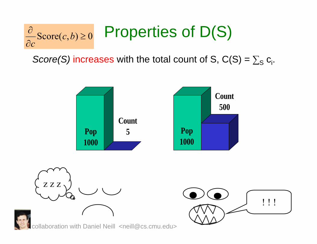
Properties of D(S)
Pop1000
Count5 Pop
1000
Count500
Score(S) increases with the total count of S, C(S) = ∑S ci.
z z z
! ! !
0),(Score ≥∂∂ bcc
collaboration with Daniel Neill <[email protected]>
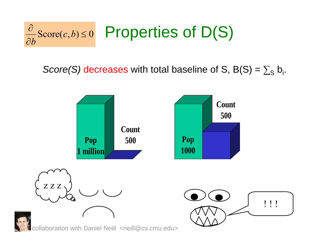
Pop1 million
Count500 Pop
1000
Count500
Properties of D(S)
Score(S) decreases with total baseline of S, B(S) = ∑S bi.
z z z
! ! !
0),(Score ≤∂∂ bcb
collaboration with Daniel Neill <[email protected]>
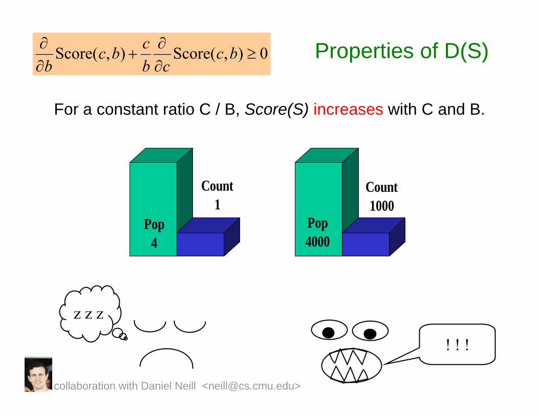
Properties of D(S)
For a constant ratio C / B, Score(S) increases with C and B.
z z z
! ! !
Pop4
Count1
Pop4000
Count1000
0),(Score),(Score ≥∂∂
+∂∂ bc
cbcbc
b
collaboration with Daniel Neill <[email protected]>
collaboration with Daniel Neill <[email protected]>
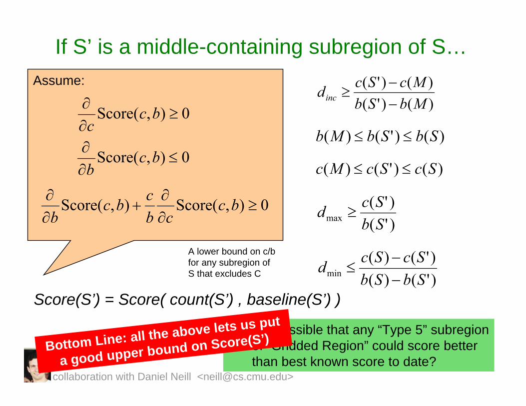
If S’ is a middle-containing subregion of S…
5. Is it possible that any “Type 5” subregionof “Gridded Region” could score better than best known score to date?
S
C
S’
Score(S’) = Score( count(S’) , baseline(S’) )
An upper bound of c/b for any subregionof S-C
An upper bound of c/b for any subregionof S that contains C
A lower bound on c/bfor any subregion of S that excludes C
Assume:
0),(Score ≥∂∂ bcc
0),(Score ≤∂∂ bcb
0),(Score),(Score ≥∂∂
+∂∂ bc
cbcbc
b
Bottom Line: all the above lets us put
a good upper bound on Score(S’)
)()'()()'(
MbSbMcScdinc −
−≥
)()'()( SbSbMb ≤≤
)()'()( ScScMc ≤≤
)'()'(
max SbScd ≥
)'()()'()(
min SbSbScScd
−−
≤
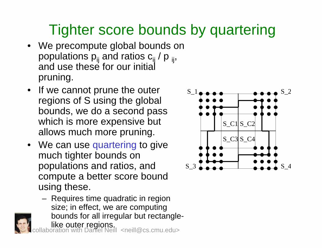
Tighter score bounds by quartering• We precompute global bounds on
populations pij and ratios cij / p ij, and use these for our initial pruning.
• If we cannot prune the outer regions of S using the global bounds, we do a second pass which is more expensive but allows much more pruning.
• We can use quartering to give much tighter bounds on populations and ratios, and compute a better score bound using these.– Requires time quadratic in region
size; in effect, we are computing bounds for all irregular but rectangle-like outer regions.
S_1 S_2
S_4S_3
S_C4
S_C1 S_C2
S_C3
collaboration with Daniel Neill <[email protected]>
Where are we?
• So we can find the most significant region by searching over the desired set of regions S, and finding the highest D(S).
• Now how can we find whether this region actually is a significant cluster?
collaboration with Daniel Neill <[email protected]>
Where are we?
• So we can find the most significant region by searching over the desired set of regions S, and finding the highest D(S).
• Now how can we find whether this region actually is a significant cluster?
• Randomization testingCan sometimes cost us 1000 times more computation!
Though there are further tricks…
collaboration with Daniel Neill <[email protected]>
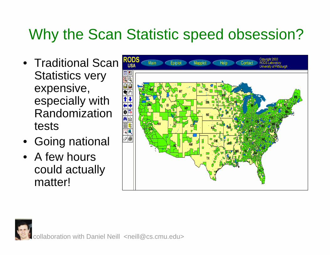
Why the Scan Statistic speed obsession?
• Traditional Scan Statistics very expensive, especially with Randomization tests
• Going national• A few hours
could actually matter!
collaboration with Daniel Neill <[email protected]>
collaboration with Daniel Neill <[email protected]>
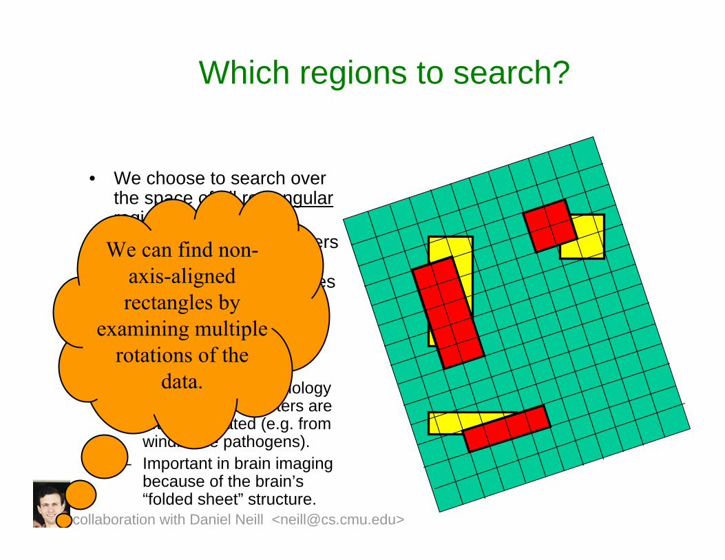
Which regions to search?
• We choose to search over the space of all rectangularregions.
• We typically expect clusters to be convex; thus inner/outer bounding boxes are reasonably close approximations to shape.
• We can find clusters with high aspect ratios.– Important in epidemiology
since disease clusters are often elongated (e.g. from windborne pathogens).
– Important in brain imaging because of the brain’s “folded sheet” structure.
We can find non-axis-aligned rectangles by
examining multiple rotations of the
data.
SC
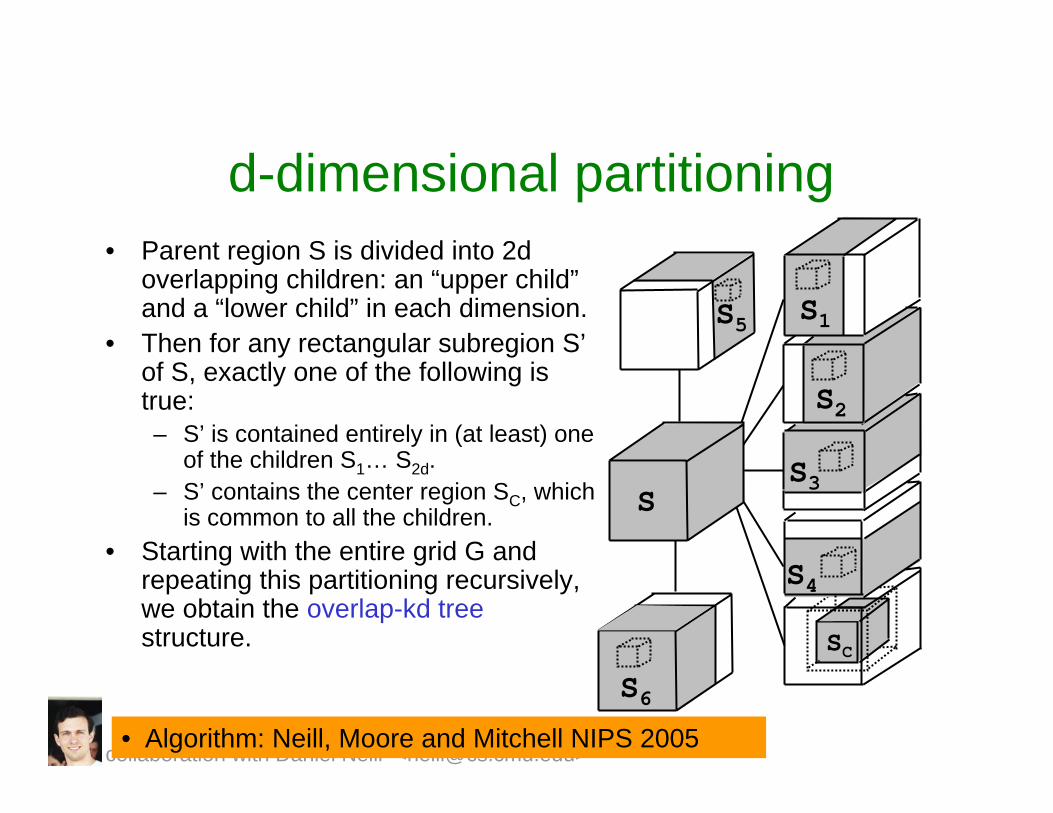
d-dimensional partitioning• Parent region S is divided into 2d
overlapping children: an “upper child”and a “lower child” in each dimension.
• Then for any rectangular subregion S’of S, exactly one of the following is true:– S’ is contained entirely in (at least) one
of the children S1… S2d.– S’ contains the center region SC, which
is common to all the children.• Starting with the entire grid G and
repeating this partitioning recursively, we obtain the overlap-kd treestructure.
S5 S1
S2
S3
S4
S6
S
collaboration with Daniel Neill <[email protected]>• Algorithm: Neill, Moore and Mitchell NIPS 2005
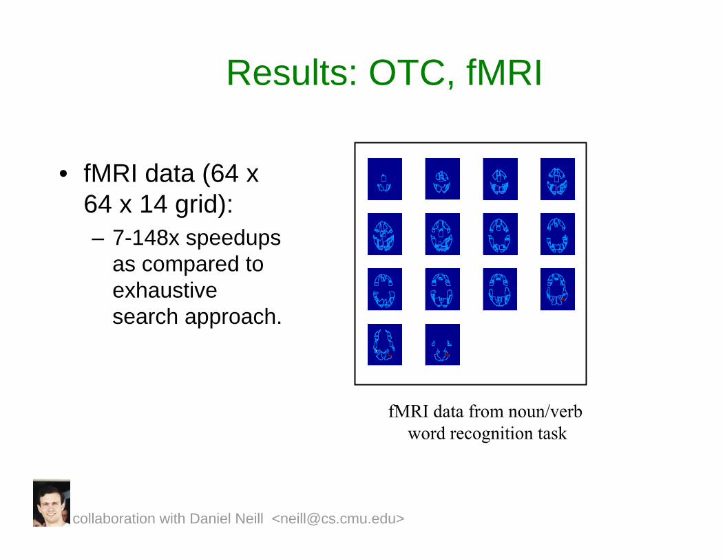
Results: OTC, fMRI
• fMRI data (64 x 64 x 14 grid):– 7-148x speedups
as compared to exhaustive search approach.
fMRI data from noun/verb word recognition task
collaboration with Daniel Neill <[email protected]>
Limitations of the algorithm
• Data must be aggregated to a grid.• Not appropriate for very high-
dimensional data.• Assumes that we are interested in
finding (rotated) rectangular regions.• Less useful for special cases (e.g.
square regions, small regions only).• Slower for finding multiple regions.
collaboration with Daniel Neill <[email protected]>
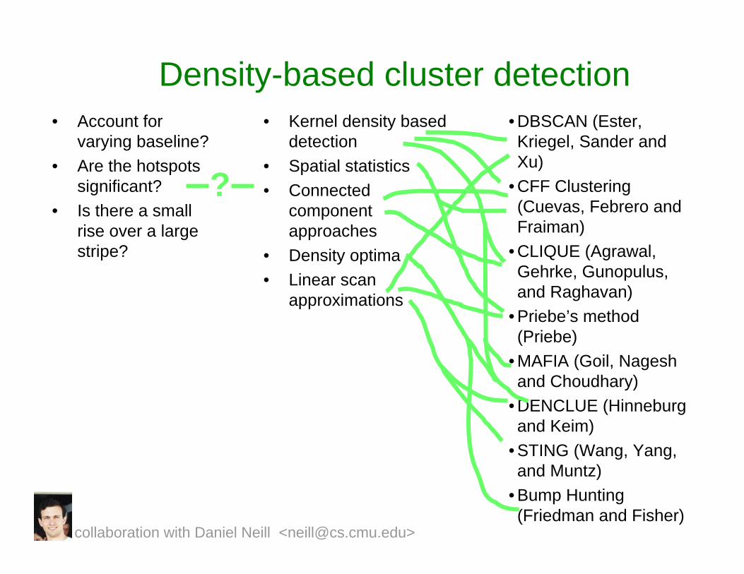
Density-based cluster detection• Kernel density based
detection• Spatial statistics• Connected
component approaches
• Density optima• Linear scan
approximations
collaboration with Daniel Neill <[email protected]>
• Kernel density based detection
• Spatial statistics• Connected
component approaches
• Density optima• Linear scan
approximations
collaboration with Daniel Neill <[email protected]>
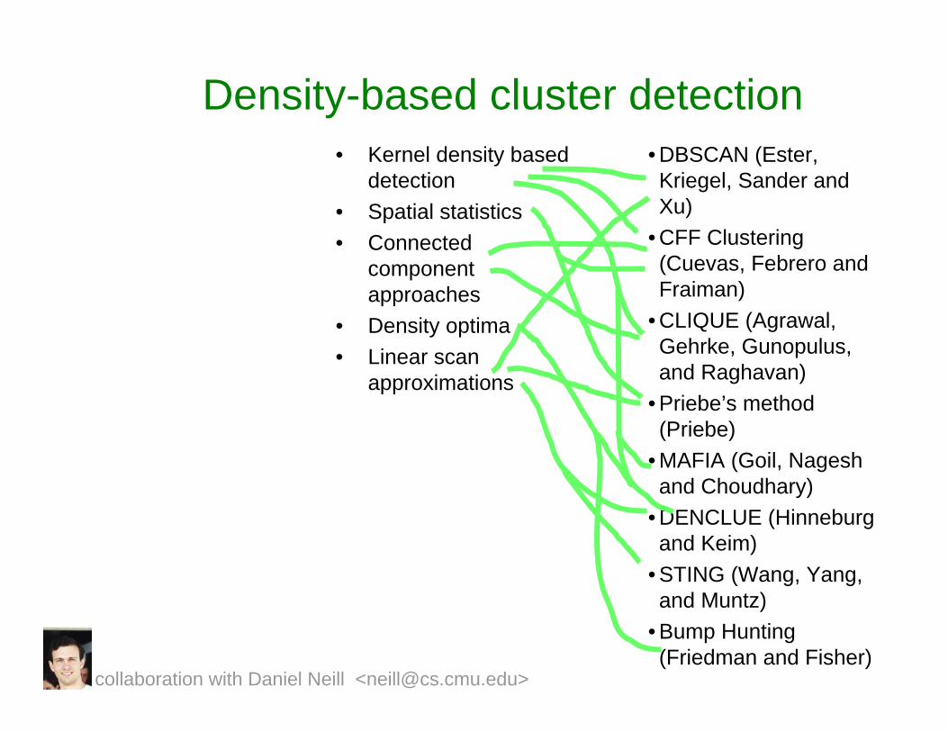
• DBSCAN (Ester, Kriegel, Sander and Xu)
• CFF Clustering (Cuevas, Febrero and Fraiman)
• CLIQUE (Agrawal, Gehrke, Gunopulus, and Raghavan)
• Priebe’s method (Priebe)
• MAFIA (Goil, Nageshand Choudhary)
• DENCLUE (Hinneburgand Keim)
• STING (Wang, Yang, and Muntz)
• Bump Hunting (Friedman and Fisher)
Density-based cluster detection
• Kernel density based detection
• Spatial statistics• Connected
component approaches
• Density optima• Linear scan
approximations
collaboration with Daniel Neill <[email protected]>
• DBSCAN (Ester, Kriegel, Sander and Xu)
• CFF Clustering (Cuevas, Febrero and Fraiman)
• CLIQUE (Agrawal, Gehrke, Gunopulus, and Raghavan)
• Priebe’s method (Priebe)
• MAFIA (Goil, Nageshand Choudhary)
• DENCLUE (Hinneburgand Keim)
• STING (Wang, Yang, and Muntz)
• Bump Hunting (Friedman and Fisher)
• Account for varying baseline?
• Are the hotspots significant?
• Is there a small rise over a large stripe?
?
Density-based cluster detection
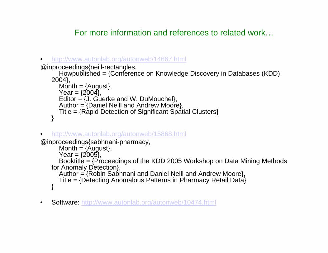
For more information and references to related work…
• http://www.autonlab.org/autonweb/14667.html@inproceedings{neill-rectangles,
Howpublished = {Conference on Knowledge Discovery in Databases (KDD) 2004},
Month = {August},Year = {2004},Editor = {J. Guerke and W. DuMouchel},Author = {Daniel Neill and Andrew Moore},Title = {Rapid Detection of Significant Spatial Clusters}
}
• http://www.autonlab.org/autonweb/15868.html@inproceedings{sabhnani-pharmacy,
Month = {August},Year = {2005},Booktitle = {Proceedings of the KDD 2005 Workshop on Data Mining Methods
for Anomaly Detection},Author = {Robin Sabhnani and Daniel Neill and Andrew Moore},Title = {Detecting Anomalous Patterns in Pharmacy Retail Data}
}
• Software: http://www.autonlab.org/autonweb/10474.html
Cached Sufficient StatisticsNew searches over cached statistics
Biosurveillance and EpidemiologyScan StatisticsCached Scan StatisticsBranch-and-Bound Scan StatisticsRetail data monitoringBrain monitoringEntering Google
AsteroidsMulti (and I mean multi) object target tracking Multiple-tree searchEntering Google
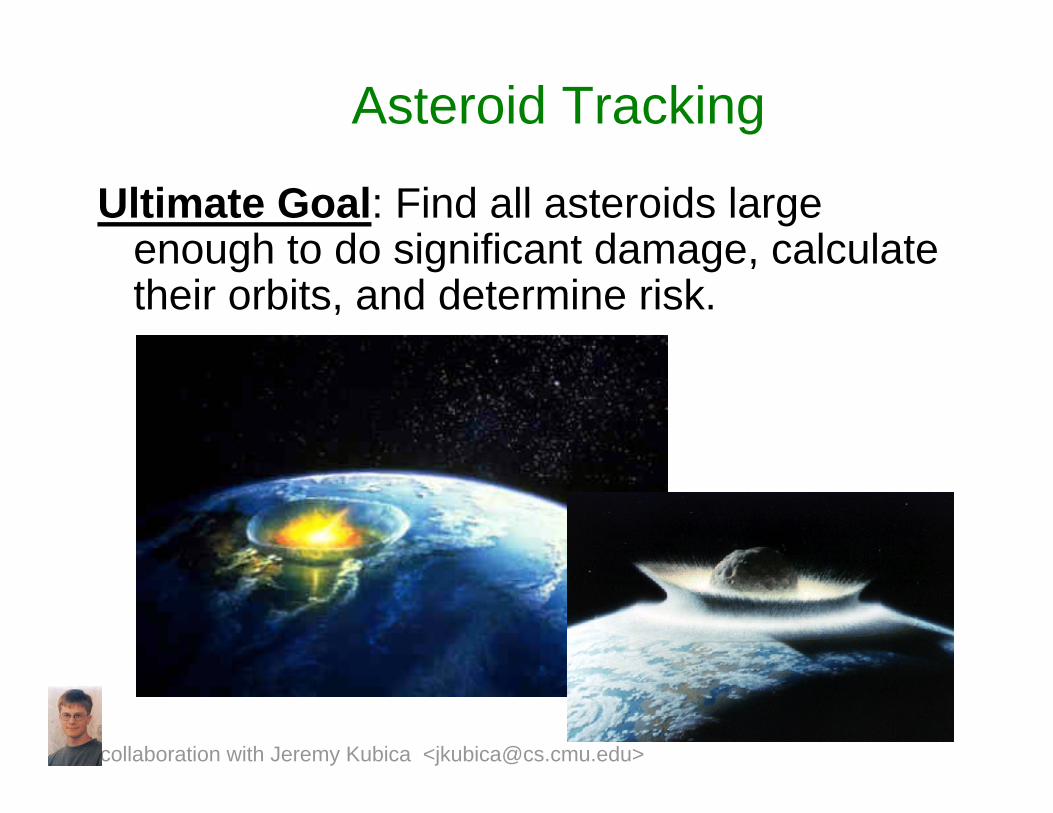
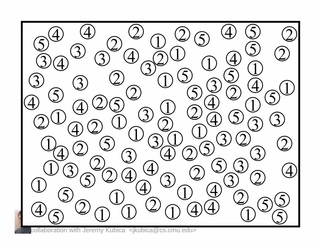
Asteroid Tracking
Ultimate Goal: Find all asteroids large enough to do significant damage, calculate their orbits, and determine risk.
collaboration with Jeremy Kubica <[email protected]>
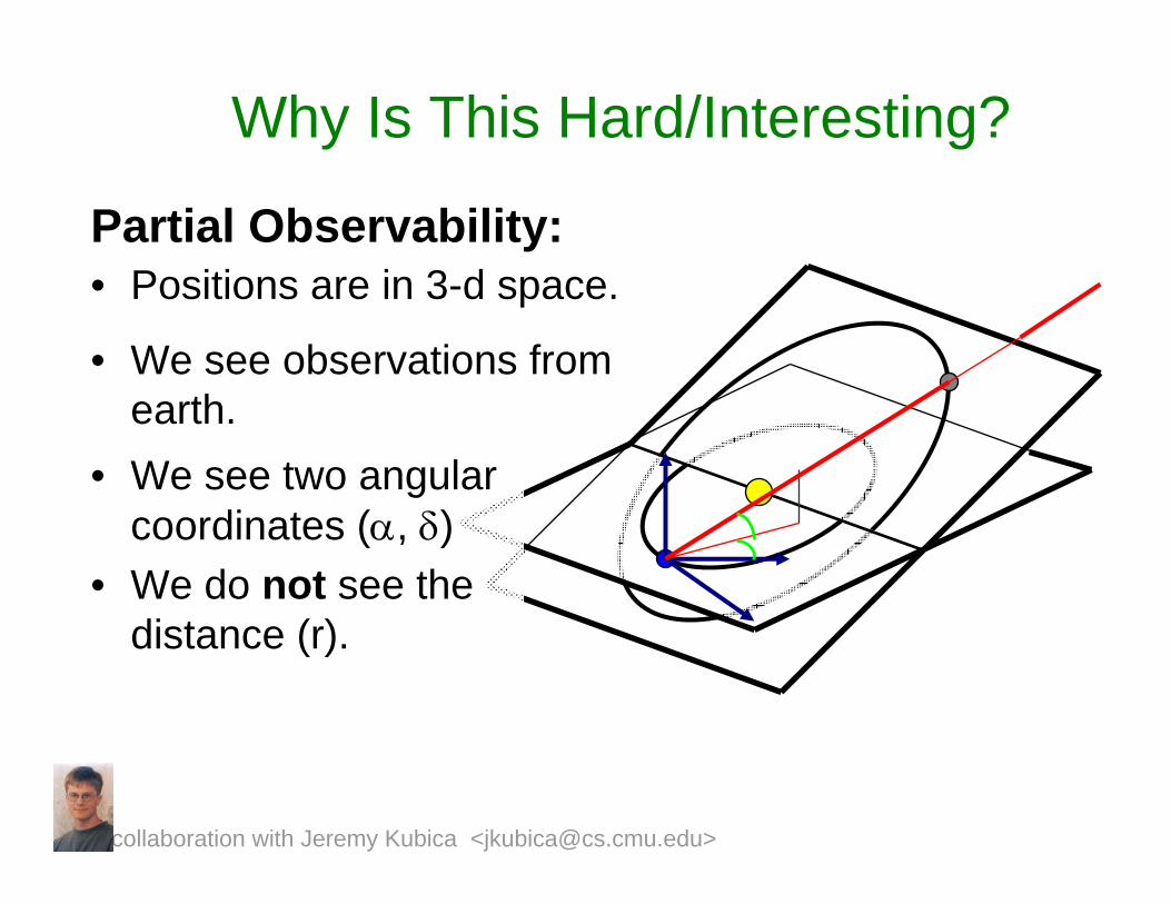
Why Is This Hard/Interesting?
Partial Observability:• Positions are in 3-d space.
• We see observations from earth.
• We see two angular coordinates (α, δ)
• We do not see the distance (r).
collaboration with Jeremy Kubica <[email protected]>
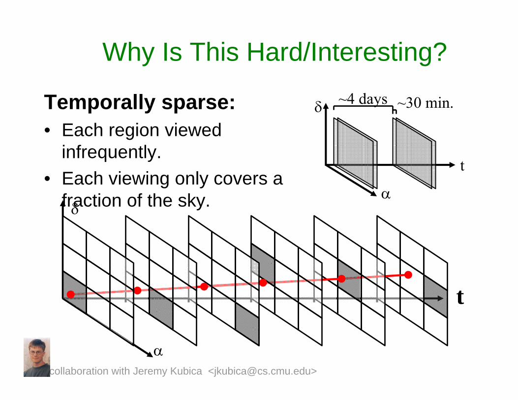
Why Is This Hard/Interesting?
Temporally sparse:• Each region viewed
infrequently. • Each viewing only covers a
fraction of the sky.
t
δ
α
~4 days ~30 min.
t
δ
α
collaboration with Jeremy Kubica <[email protected]>
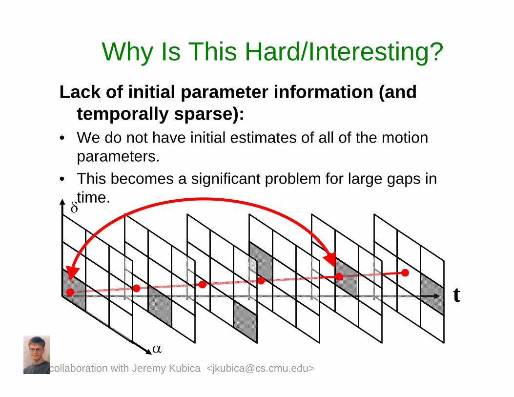
Why Is This Hard/Interesting?Lack of initial parameter information (and
temporally sparse):• We do not have initial estimates of all of the motion
parameters.• This becomes a significant problem for large gaps in
time.δ
t
αcollaboration with Jeremy Kubica <[email protected]>
collaboration with Jeremy Kubica <[email protected]>
13
4 52
13 4 5
21
3
4
5
21
34
5
2
1
3 4
5
2
1
3
4
5
2
4
444
4
3 3
3
2
2
2
22
5
5
5
55
5
43 3
13
4
2
5
5
12
1
1
1
1
14 5
134 2
13
3
4
251
122
22
4
4
5
4
23
32
2
52141
3
4 5
1
1
5
1
2
2
4
collaboration with Jeremy Kubica <[email protected]>
13
4 52
13 4 5
21
3
4
5
21
34
5
2
1
3 4
5
2
1
3
4
5
2
4
444
4
3 3
3
2
2
2
22
5
5
5
55
5
43 3
13
4
2
5
5
12
1
1
1
1
14 5
134 2
13
3
4
251
122
22
4
4
5
4
23
32
2
52141
3
4 5
1
1
5
1
2
2
4
collaboration with Jeremy Kubica <[email protected]>
13
4 52
13 4 5
21
3
4
5
21
34
5
2
1
3 4
5
2
1
3
4
5
2
4
444
4
3 3
3
2
2
2
22
5
5
5
55
5
43 3
13
4
2
5
5
12
1
1
1
1
14 5
134 2
13
3
4
251
122
22
4
4
5
4
23
32
2
52141
3
4 5
1
1
5
1
2
2
4
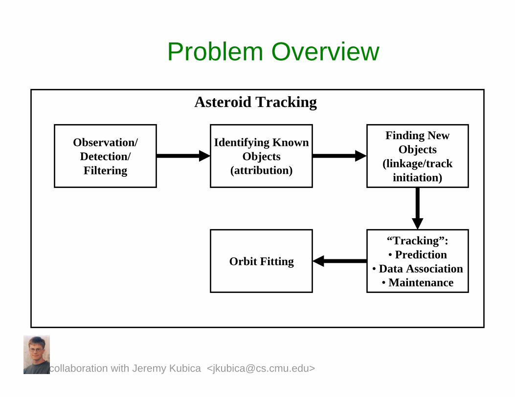
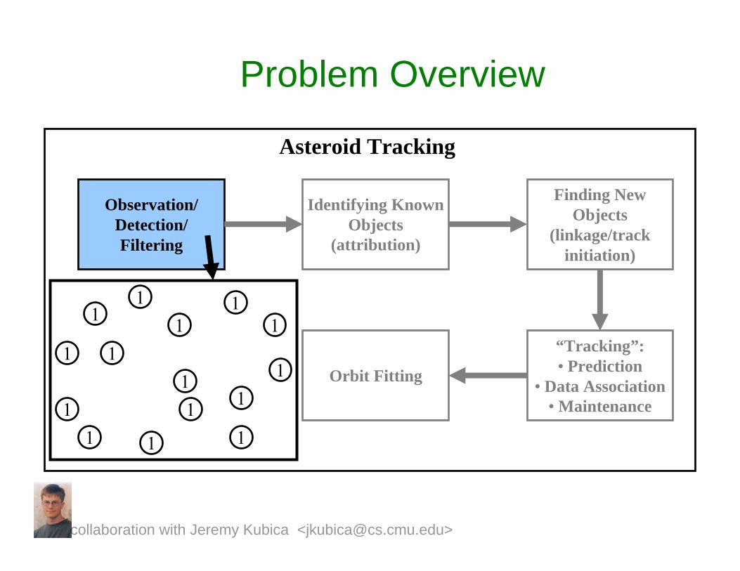
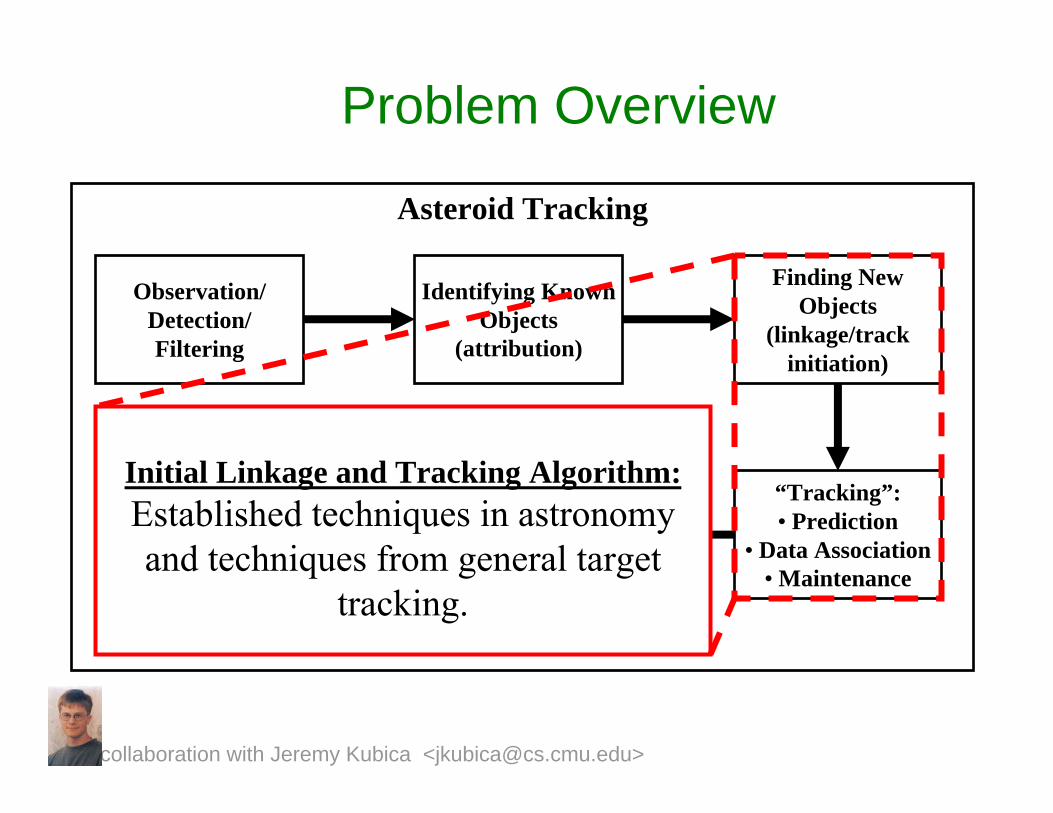
Problem Overview
Asteroid Tracking
Observation/Detection/Filtering
Identifying Known Objects
(attribution)
Finding New Objects
(linkage/track initiation)
“Tracking”:• Prediction
• Data Association• Maintenance
Orbit Fitting
collaboration with Jeremy Kubica <[email protected]>
Problem Overview
Asteroid Tracking
Observation/Detection/Filtering
Identifying Known Objects
(attribution)
Finding New Objects
(linkage/track initiation)
“Tracking”:• Prediction
• Data Association• Maintenance
Orbit Fitting
1
1 1
11
1
1
1
1
1
1
1
1
11
collaboration with Jeremy Kubica <[email protected]>
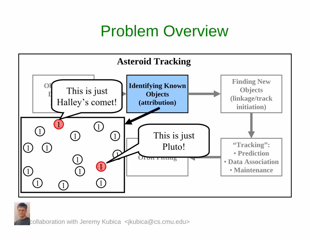
Problem Overview
Asteroid Tracking
Observation/Detection/Filtering
Identifying Known Objects
(attribution)
Finding New Objects
(linkage/track initiation)
“Tracking”:• Prediction
• Data Association• Maintenance
Orbit Fitting1
1
1
1 1
11
1
1
1
1
1
1
11
1
11
1
This is just Halley’s comet!
This is just Pluto!
collaboration with Jeremy Kubica <[email protected]>

Problem Overview
Asteroid Tracking
Observation/Detection/Filtering
Identifying Known Objects
(attribution)
Finding New Objects
(linkage/track initiation)
“Tracking”:• Prediction
• Data Association• Maintenance
Orbit Fitting
1 1
11
1
1
1
1
1
1
11
2
2
2
2
2
3 3
3
3
3
3
3
3 3
2
2
2
2
3
23
112
3
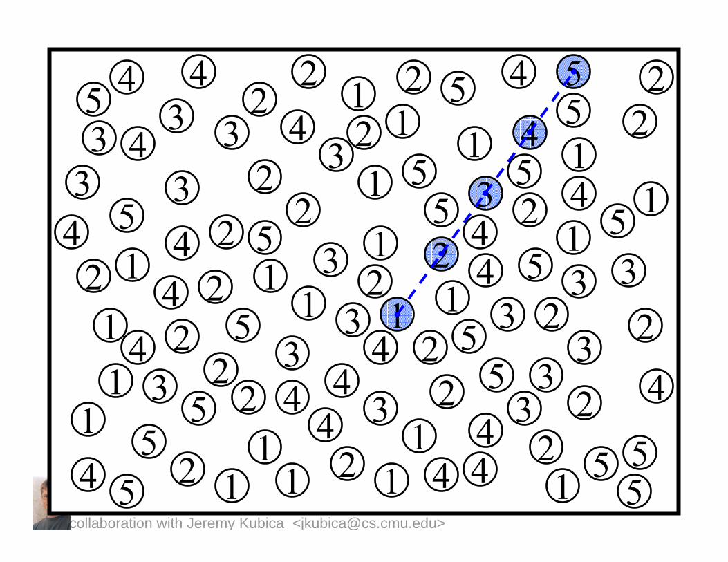
This looks like it could be the start
of a track!
collaboration with Jeremy Kubica <[email protected]>
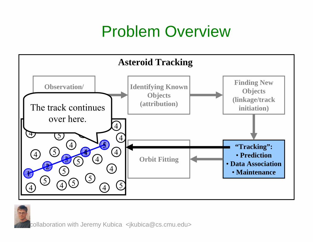
Problem Overview
Asteroid Tracking
Observation/Detection/Filtering
Identifying Known Objects
(attribution)
Finding New Objects
(linkage/track initiation)
“Tracking”:• Prediction
• Data Association• Maintenance
Orbit Fitting
4
44
4
44
44
4
4
5
55
5
5
5
5
5
55
4
44
12
34
544
5
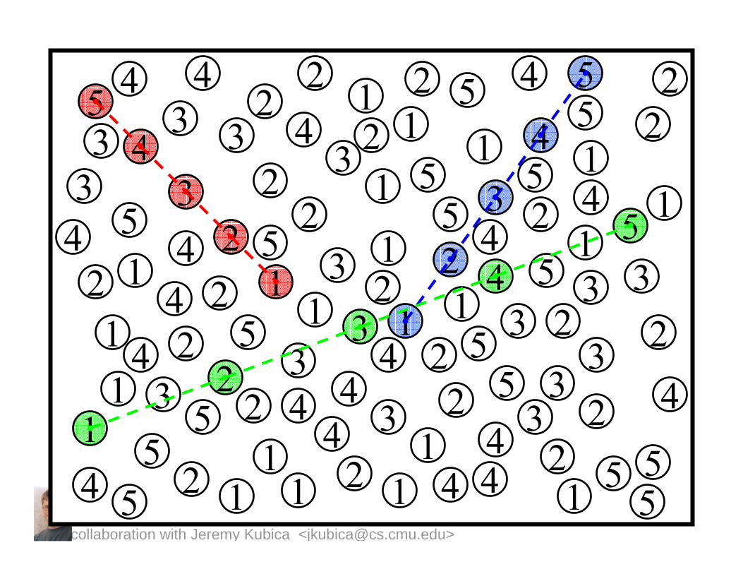
The track continues over here.
collaboration with Jeremy Kubica <[email protected]>
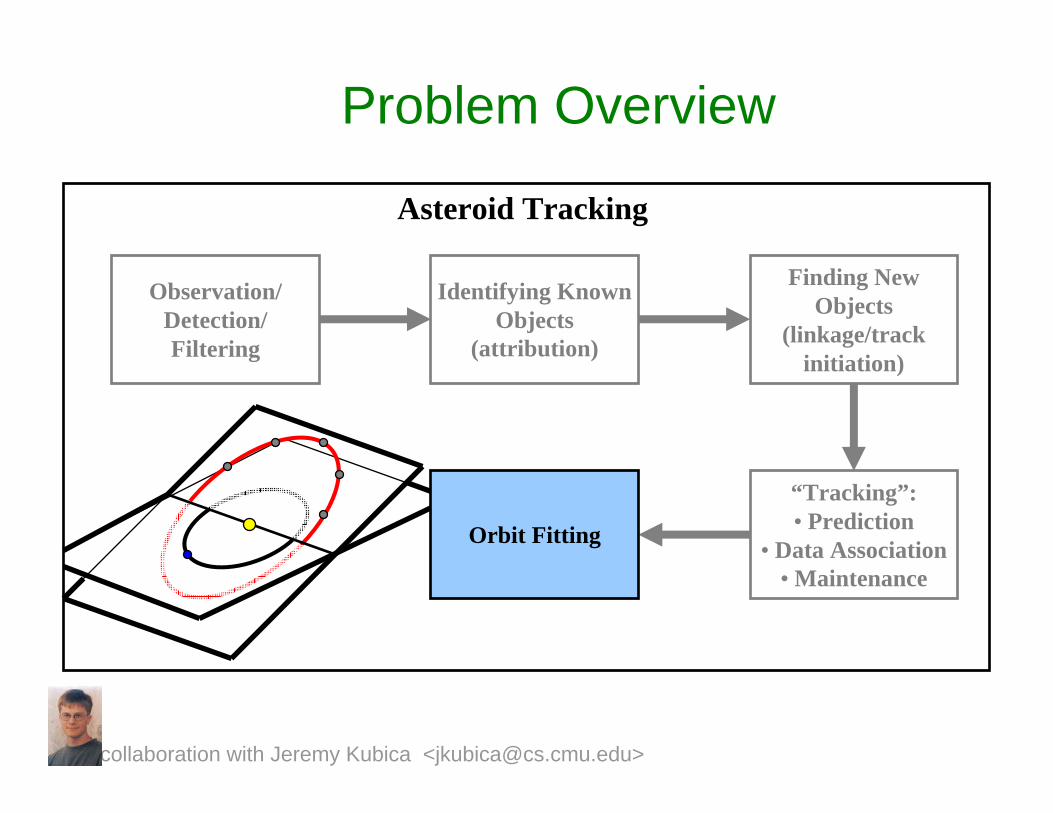
Problem Overview
Asteroid Tracking
Observation/Detection/Filtering
Identifying Known Objects
(attribution)
Finding New Objects
(linkage/track initiation)
“Tracking”:• Prediction
• Data Association• Maintenance
Orbit Fitting
collaboration with Jeremy Kubica <[email protected]>
Problem Overview
Asteroid Tracking
Observation/Detection/Filtering
Identifying Known Objects
(attribution)
Finding New Objects
(linkage/track initiation)
“Tracking”:• Prediction
• Data Association• Maintenance
Orbit Fitting
Initial Linkage and Tracking Algorithm:Established techniques in astronomy and techniques from general target
tracking.
collaboration with Jeremy Kubica <[email protected]>
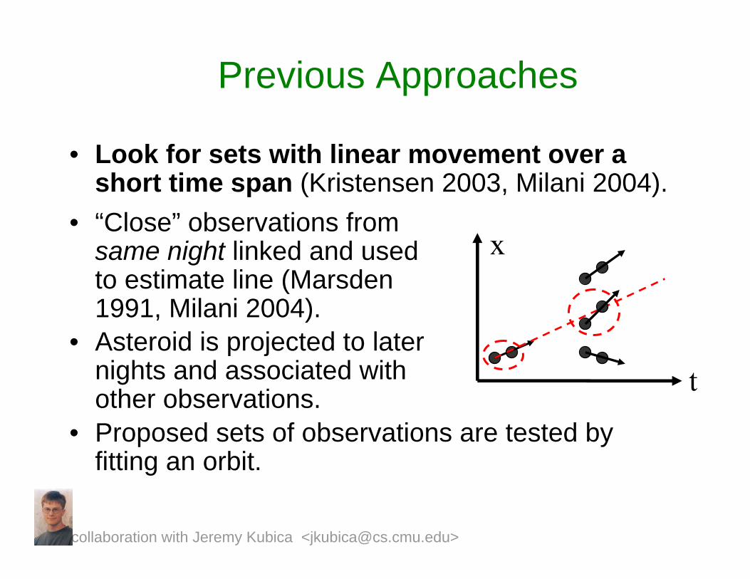
Previous Approaches
• Look for sets with linear movement over a short time span (Kristensen 2003, Milani 2004).
t
x
• Proposed sets of observations are tested by fitting an orbit.
• “Close” observations from same night linked and used to estimate line (Marsden1991, Milani 2004).
• Asteroid is projected to later nights and associated with other observations.
collaboration with Jeremy Kubica <[email protected]>
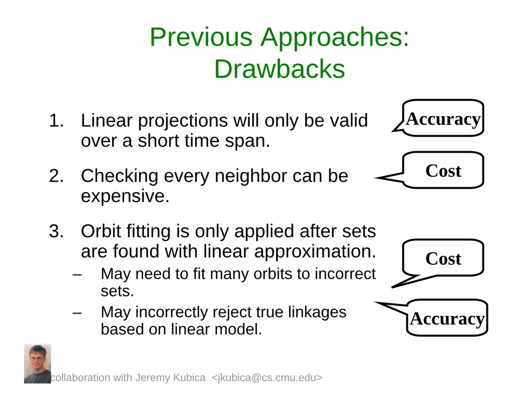
Previous Approaches: Drawbacks
1. Linear projections will only be valid over a short time span.
2. Checking every neighbor can be expensive.
3. Orbit fitting is only applied after sets are found with linear approximation.
– May need to fit many orbits to incorrect sets.
– May incorrectly reject true linkages based on linear model.
Accuracy
Cost
Cost
Accuracy
collaboration with Jeremy Kubica <[email protected]>
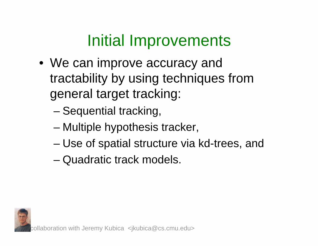
Initial Improvements• We can improve accuracy and
tractability by using techniques from general target tracking:– Sequential tracking,– Multiple hypothesis tracker, – Use of spatial structure via kd-trees, and– Quadratic track models.
collaboration with Jeremy Kubica <[email protected]>
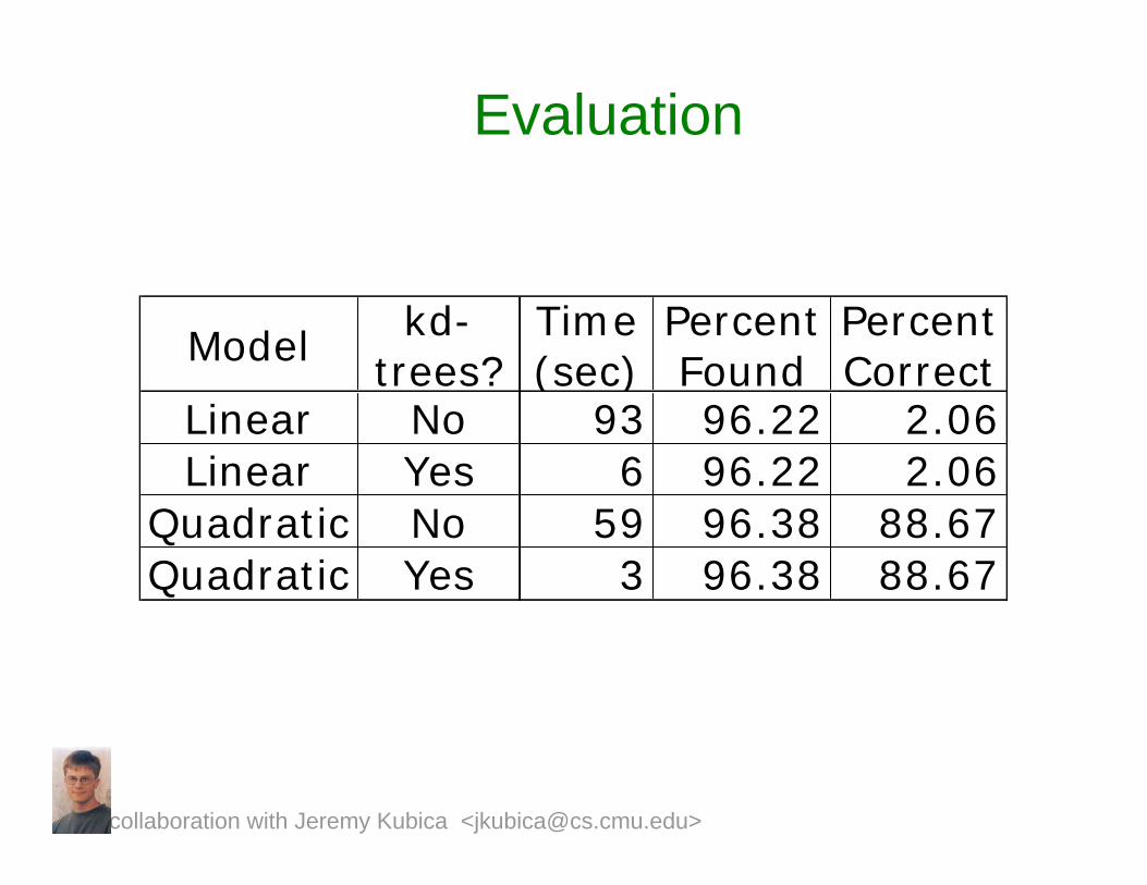
Evaluation
Modelkd-
trees?Time (sec)
Percent Found
Percent Correct
Linear No 93 96.22 2.06Linear Yes 6 96.22 2.06
Quadratic No 59 96.38 88.67Quadratic Yes 3 96.38 88.67
collaboration with Jeremy Kubica <[email protected]>
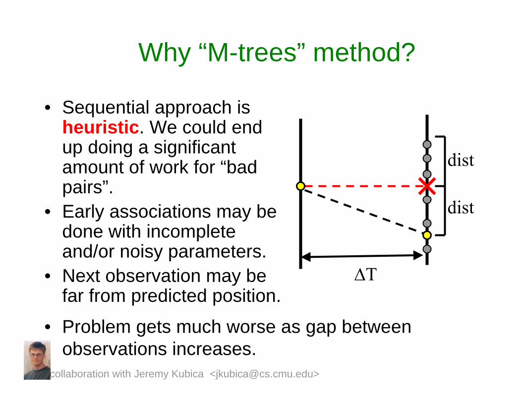
Why “M-trees” method?
• Sequential approach is heuristic. We could end up doing a significant amount of work for “bad pairs”.
• Early associations may be done with incomplete and/or noisy parameters.
• Next observation may be far from predicted position.
dist
dist
ΔT
• Problem gets much worse as gap between observations increases.
collaboration with Jeremy Kubica <[email protected]>
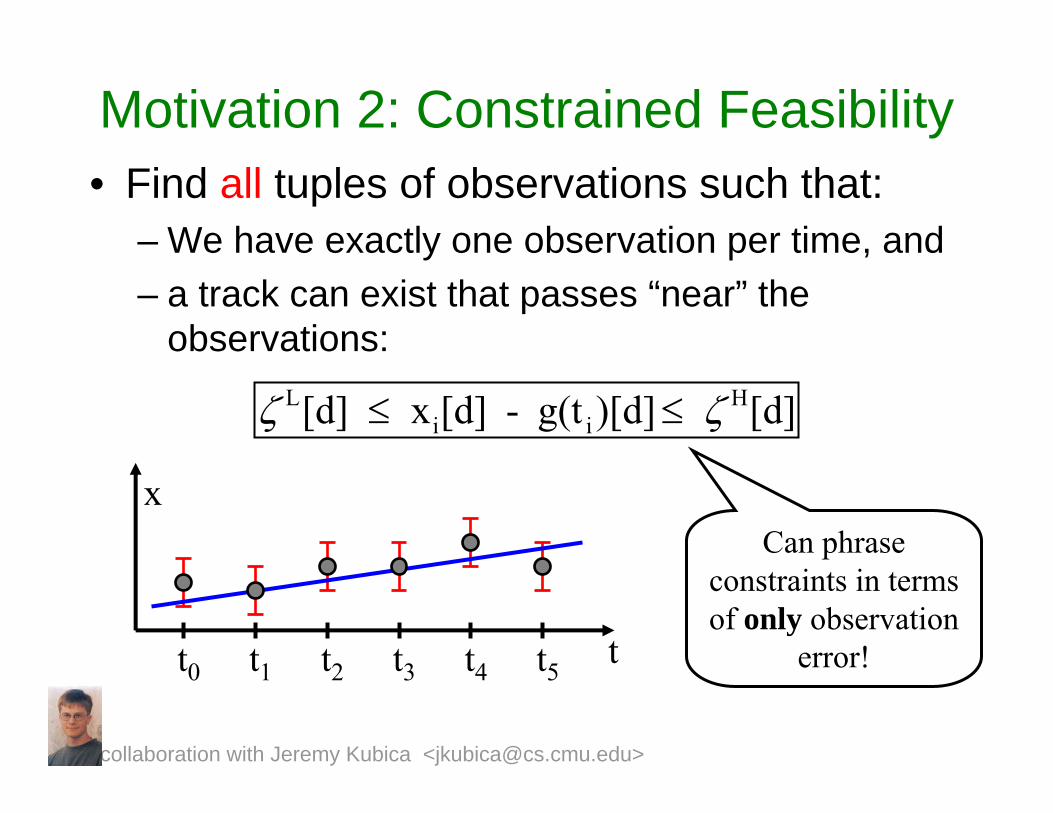
Motivation 2: Constrained Feasibility• Find all tuples of observations such that:
– We have exactly one observation per time, and– a track can exist that passes “near” the
observations:
ζ L[d] ≤ xi[d] - g(t i )[d]≤ ζ H[d]
x
tt0 t1 t2 t3 t4 t5
Can phrase constraints in terms of only observation
error!
collaboration with Jeremy Kubica <[email protected]>
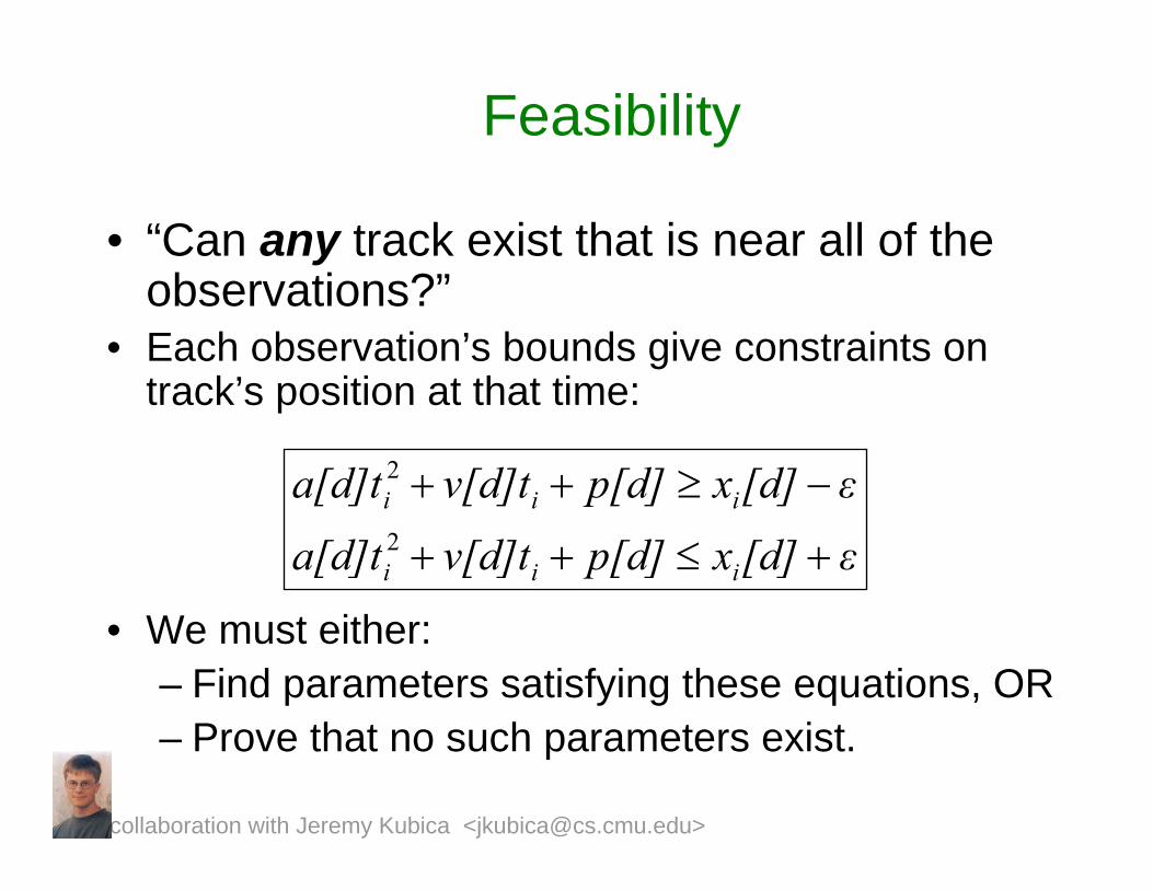
Feasibility
• “Can any track exist that is near all of the observations?”
• Each observation’s bounds give constraints on track’s position at that time:
• We must either:– Find parameters satisfying these equations, OR– Prove that no such parameters exist.
ε[d]xp[d]v[d]ta[d]t
ε[d]xp[d]v[d]ta[d]t
iii
iii
+≤++
−≥++2
2
collaboration with Jeremy Kubica <[email protected]>
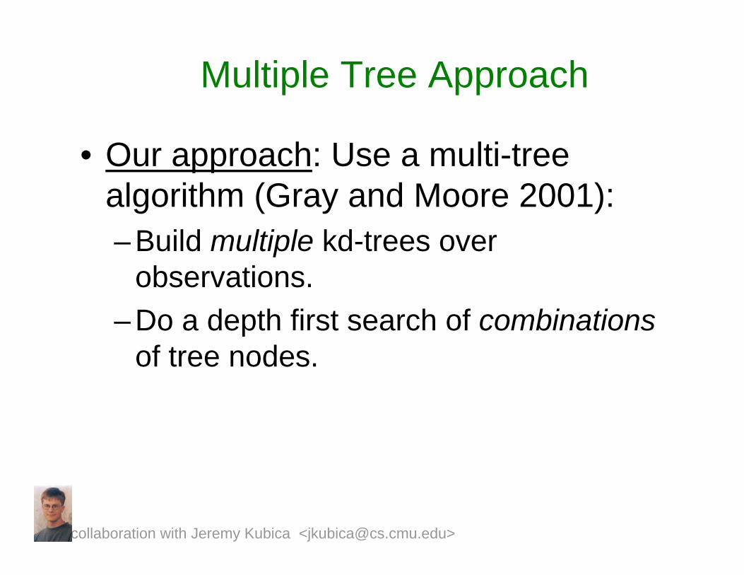
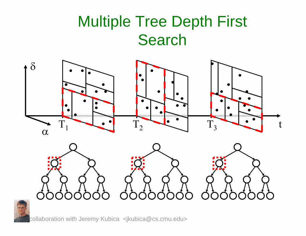
Multiple Tree Approach
• Our approach: Use a multi-tree algorithm (Gray and Moore 2001):– Build multiple kd-trees over
observations.– Do a depth first search of combinations
of tree nodes.
collaboration with Jeremy Kubica <[email protected]>
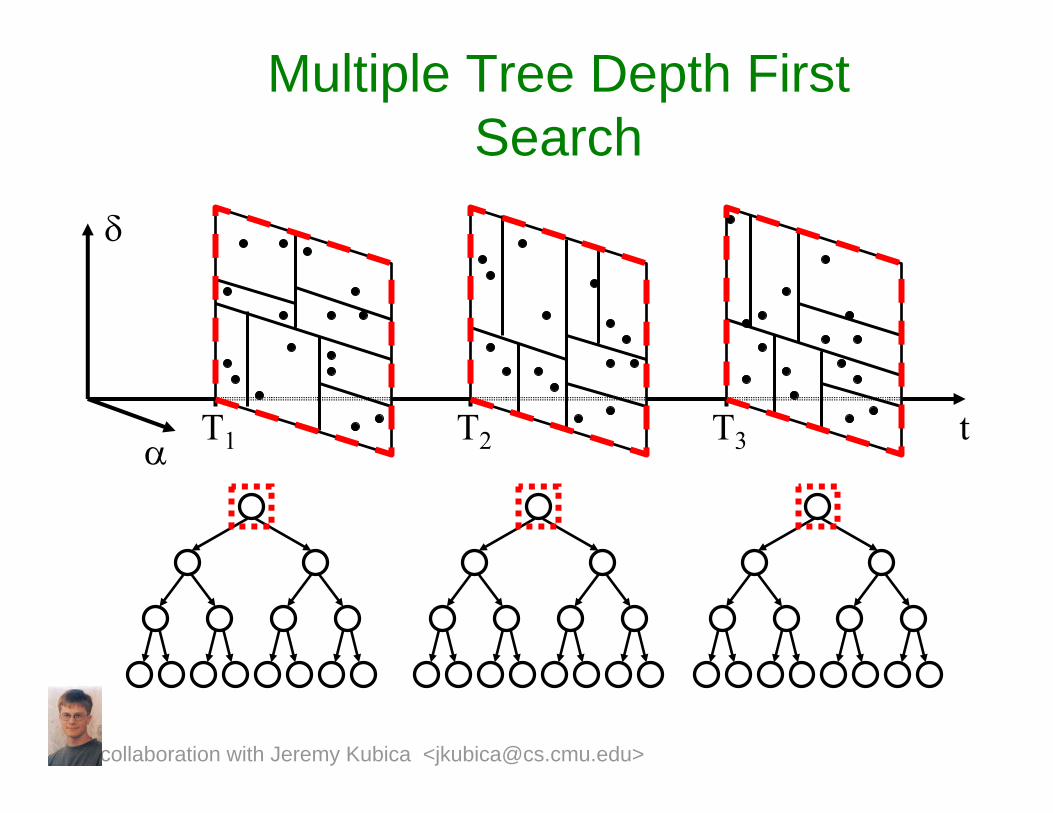
T1 T2 T3
Multiple Tree Depth First Search
t
δ
α
collaboration with Jeremy Kubica <[email protected]>
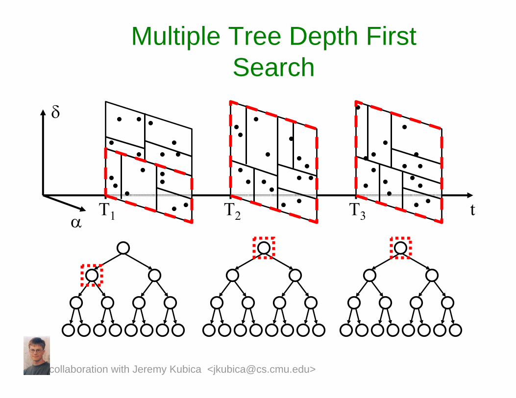
T1 T2 T3
Multiple Tree Depth First Search
t
δ
α
collaboration with Jeremy Kubica <[email protected]>
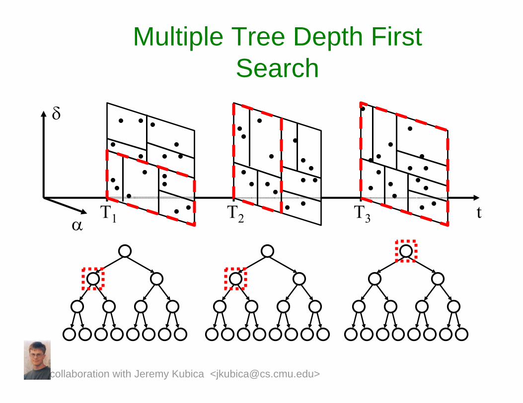
T1 T2 T3
Multiple Tree Depth First Search
t
δ
α
collaboration with Jeremy Kubica <[email protected]>
T1 T2 T3
Multiple Tree Depth First Search
t
δ
α
collaboration with Jeremy Kubica <[email protected]>
T1 T2 T3
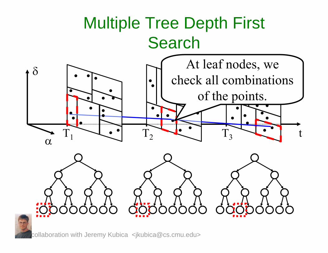
Multiple Tree Depth First Search
t
At leaf nodes, we check all combinations
of the points.
δ
α
collaboration with Jeremy Kubica <[email protected]>
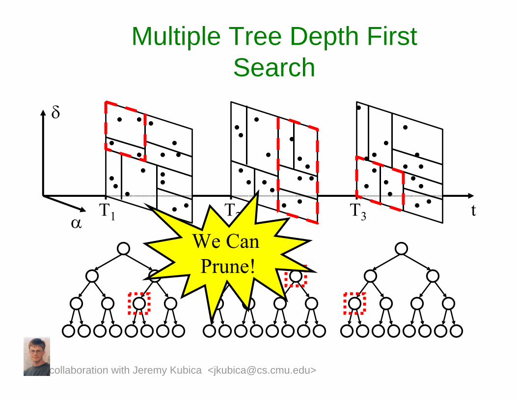
T1 T2 T3
Multiple Tree Depth First Search
We Can Prune!
t
δ
α
collaboration with Jeremy Kubica <[email protected]>
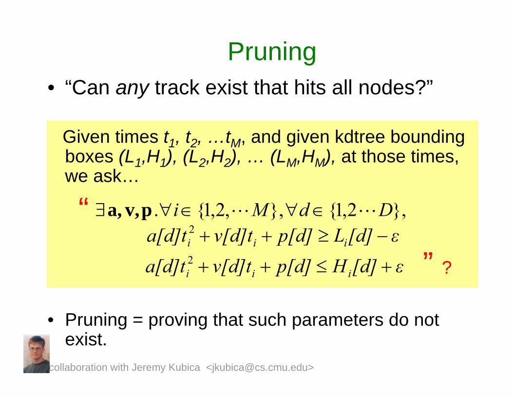
Pruning• “Can any track exist that hits all nodes?”
Given times t1, t2, …tM, and given kdtree bounding boxes (L1,H1), (L2,H2), … (LM,HM), at those times, we ask…
• Pruning = proving that such parameters do not exist.
collaboration with Jeremy Kubica <[email protected]>
ε[d]Hp[d]v[d]ta[d]t iii +≤++2
ε[d]Lp[d]v[d]ta[d]t iii −≥++2},2,1{},,2,1{. DdMi LL ∈∀∈∀∃ pv,a,
” ?
“
collaboration with Jeremy Kubica <[email protected]>
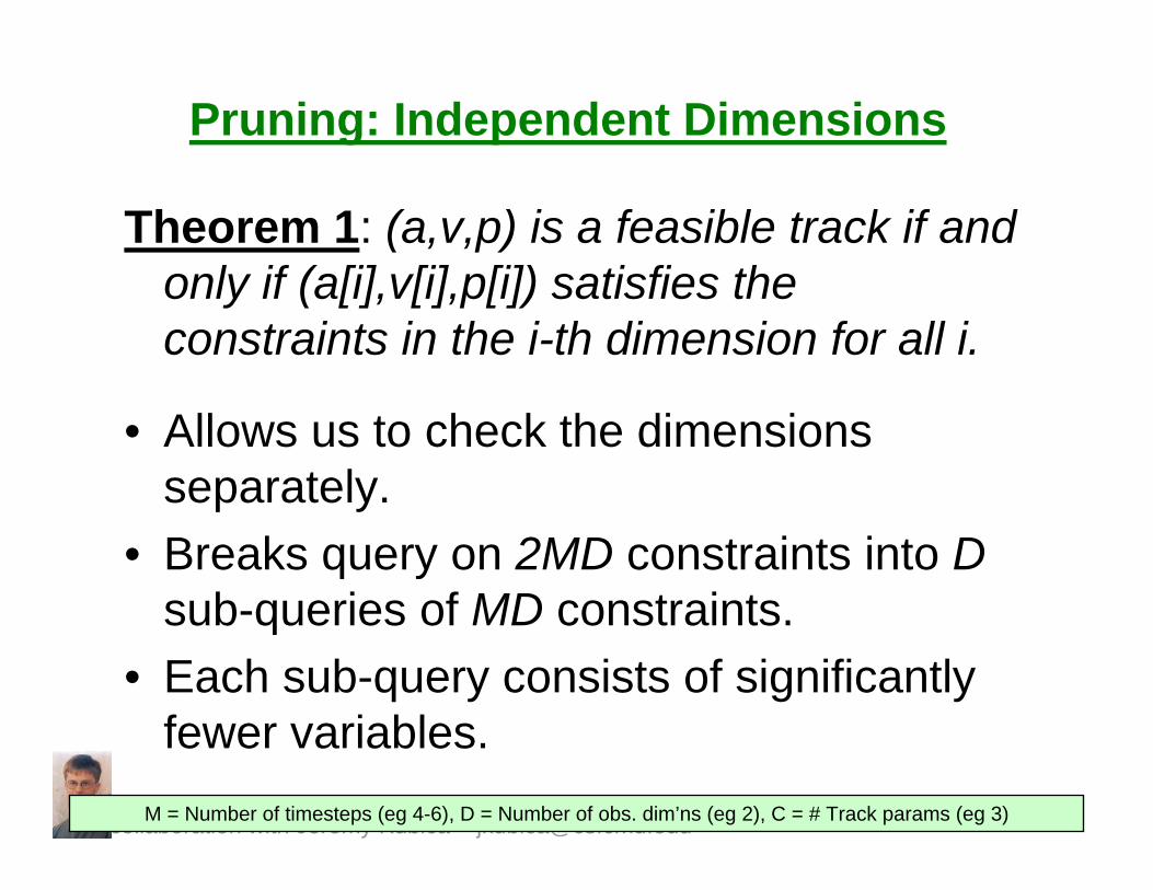
Pruning: Independent Dimensions
Theorem 1: (a,v,p) is a feasible track if and only if (a[i],v[i],p[i]) satisfies the constraints in the i-th dimension for all i.
• Allows us to check the dimensions separately.
• Breaks query on 2MD constraints into Dsub-queries of MD constraints.
• Each sub-query consists of significantly fewer variables.
M = Number of timesteps (eg 4-6), D = Number of obs. dim’ns (eg 2), C = # Track params (eg 3)
collaboration with Jeremy Kubica <[email protected]>
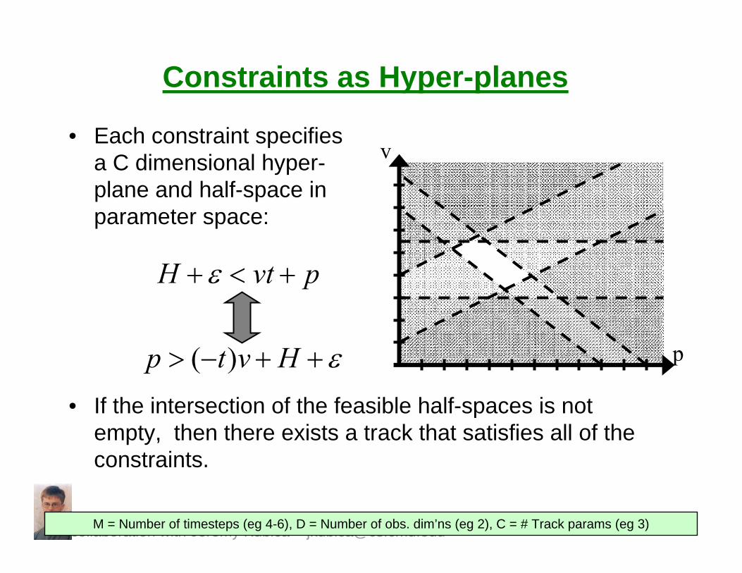
Constraints as Hyper-planes
• Each constraint specifies a C dimensional hyper-plane and half-space in parameter space:
p
v
• If the intersection of the feasible half-spaces is not empty, then there exists a track that satisfies all of the constraints.
pvtH +<+ε
ε++−> Hvtp )(
M = Number of timesteps (eg 4-6), D = Number of obs. dim’ns (eg 2), C = # Track params (eg 3)
collaboration with Jeremy Kubica <[email protected]>
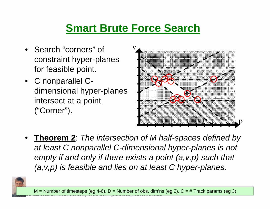
Smart Brute Force Search
• Search “corners” of constraint hyper-planes for feasible point.
• C nonparallel C-dimensional hyper-planes intersect at a point (“Corner”).
p
v
• Theorem 2: The intersection of M half-spaces defined by at least C nonparallel C-dimensional hyper-planes is not empty if and only if there exists a point (a,v,p) such that (a,v,p) is feasible and lies on at least C hyper-planes.
M = Number of timesteps (eg 4-6), D = Number of obs. dim’ns (eg 2), C = # Track params (eg 3)
collaboration with Jeremy Kubica <[email protected]>
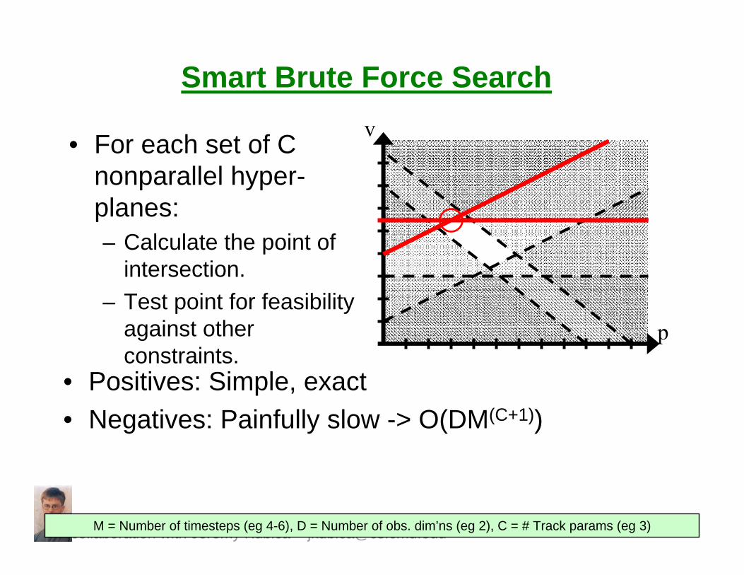
Smart Brute Force Search
• For each set of C nonparallel hyper-planes:– Calculate the point of
intersection.– Test point for feasibility
against other constraints.
p
v
• Positives: Simple, exact• Negatives: Painfully slow -> O(DM(C+1))
M = Number of timesteps (eg 4-6), D = Number of obs. dim’ns (eg 2), C = # Track params (eg 3)
collaboration with Jeremy Kubica <[email protected]>
Using Structure In the Search
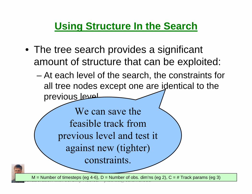
• The tree search provides a significant amount of structure that can be exploited:– At each level of the search, the constraints for
all tree nodes except one are identical to the previous level.
We can save the feasible track from
previous level and test it against new (tighter)
constraints.M = Number of timesteps (eg 4-6), D = Number of obs. dim’ns (eg 2), C = # Track params (eg 3)
collaboration with Jeremy Kubica <[email protected]>
Using Structure In the Search
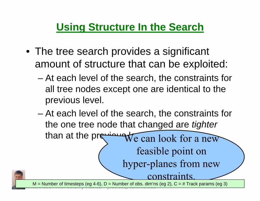
• The tree search provides a significant amount of structure that can be exploited:– At each level of the search, the constraints for
all tree nodes except one are identical to the previous level.
– At each level of the search, the constraints for the one tree node that changed are tighterthan at the previous level.We can look for a new
feasible point on hyper-planes from new
constraints.M = Number of timesteps (eg 4-6), D = Number of obs. dim’ns (eg 2), C = # Track params (eg 3)
collaboration with Jeremy Kubica <[email protected]>
Using Structure In the Search
Theorem 3: If the feasible track from the previous level is not compatible with a new constraint then either the new set of constraints is not compatible or a new feasible point lies on the plane defined by the new constraint.
• Allows us to only check corners containing new constraints -> O(DMC)
• Allows us to check new constraints one at a time.
M = Number of timesteps (eg 4-6), D = Number of obs. dim’ns (eg 2), C = # Track params (eg 3)
collaboration with Jeremy Kubica <[email protected]>
Using Structure In the Search
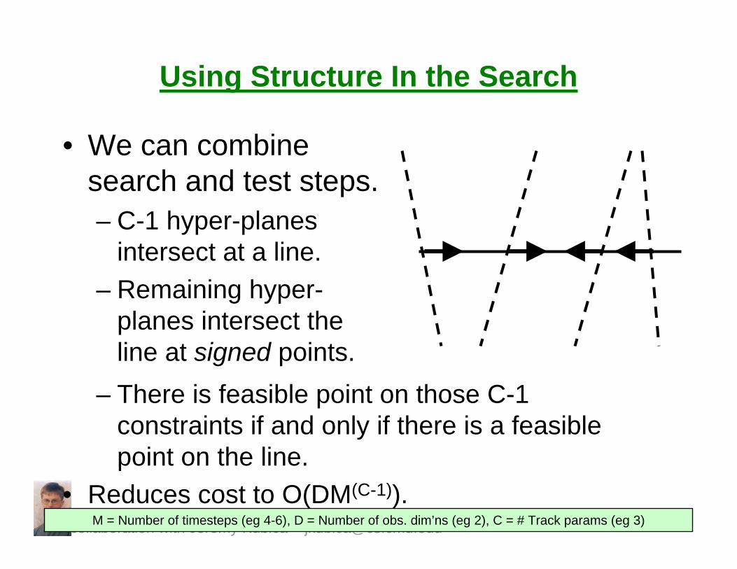
• We can combine search and test steps.– C-1 hyper-planes
intersect at a line.– Remaining hyper-
planes intersect the line at signed points.
– There is feasible point on those C-1 constraints if and only if there is a feasible point on the line.
• Reduces cost to O(DM(C-1)).M = Number of timesteps (eg 4-6), D = Number of obs. dim’ns (eg 2), C = # Track params (eg 3)
collaboration with Jeremy Kubica <[email protected]>
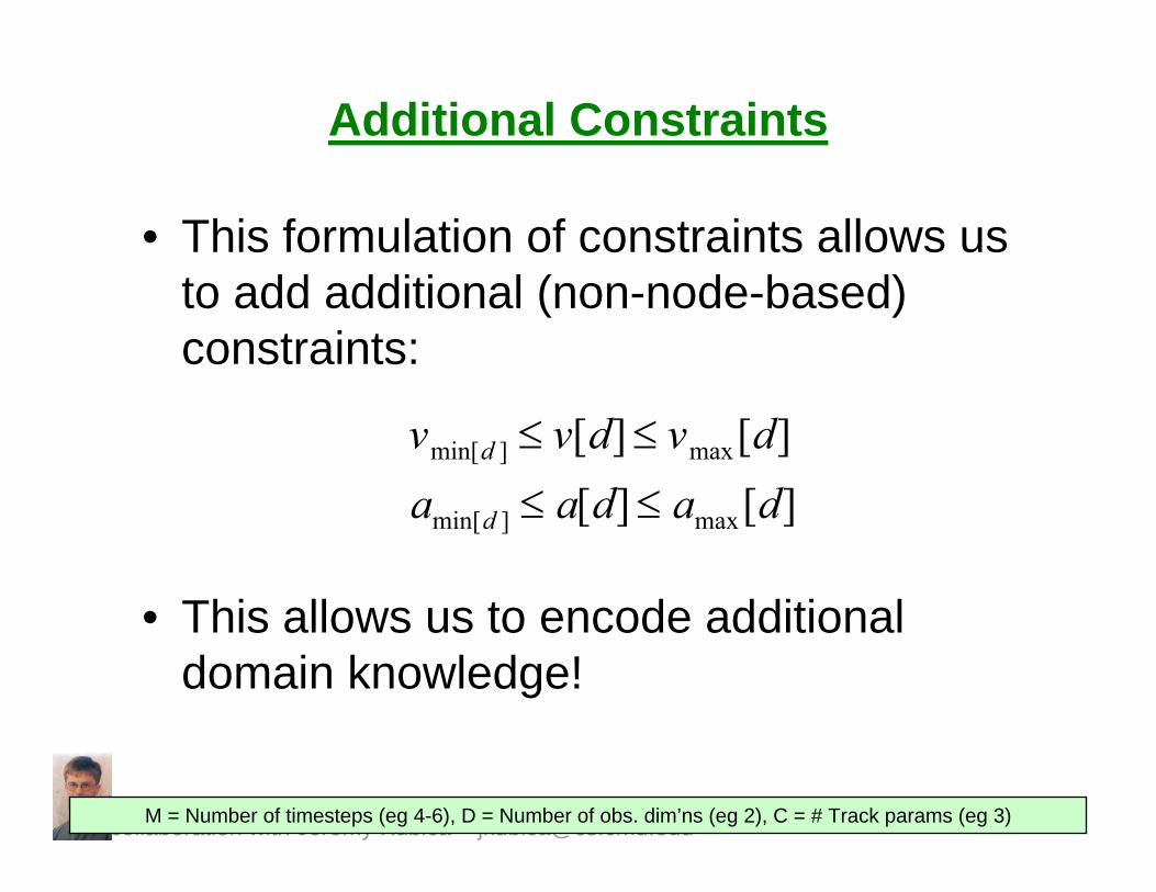
Additional Constraints
• This formulation of constraints allows us to add additional (non-node-based) constraints:
• This allows us to encode additional domain knowledge!
vmin[d ] ≤ v[d] ≤ vmax[d]amin[d ] ≤ a[d] ≤ amax[d]
M = Number of timesteps (eg 4-6), D = Number of obs. dim’ns (eg 2), C = # Track params (eg 3)
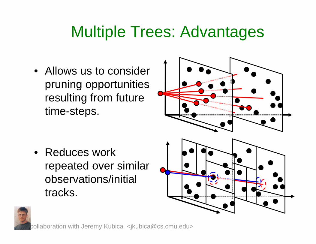
Multiple Trees: Advantages
• Allows us to consider pruning opportunities resulting from future time-steps.
• Reduces work repeated over similar observations/initial tracks.
collaboration with Jeremy Kubica <[email protected]>
collaboration with Jeremy Kubica <[email protected]>
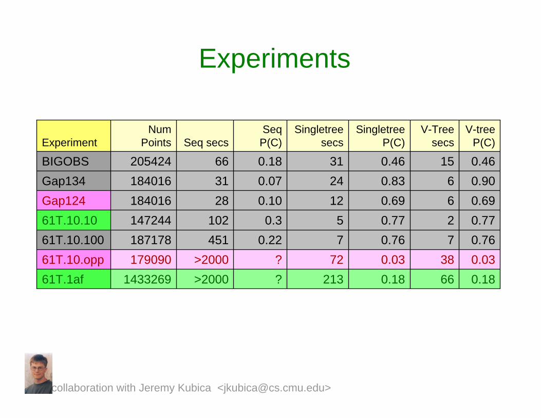
Experiments
0.180.030.760.770.690.830.46
Singletree P(C)
21372
75
122431
Singletree secs
0.7720.310214724461T.10.100.6960.1028184016Gap1240.9060.0731184016Gap134
V-tree P(C)
V-Tree secs
SeqP(C)Seq secs
Num PointsExperiment
0.1866?>2000143326961T.1af0.0338?>200017909061T.10.opp0.7670.2245118717861T.10.100
0.46150.1866205424BIGOBS

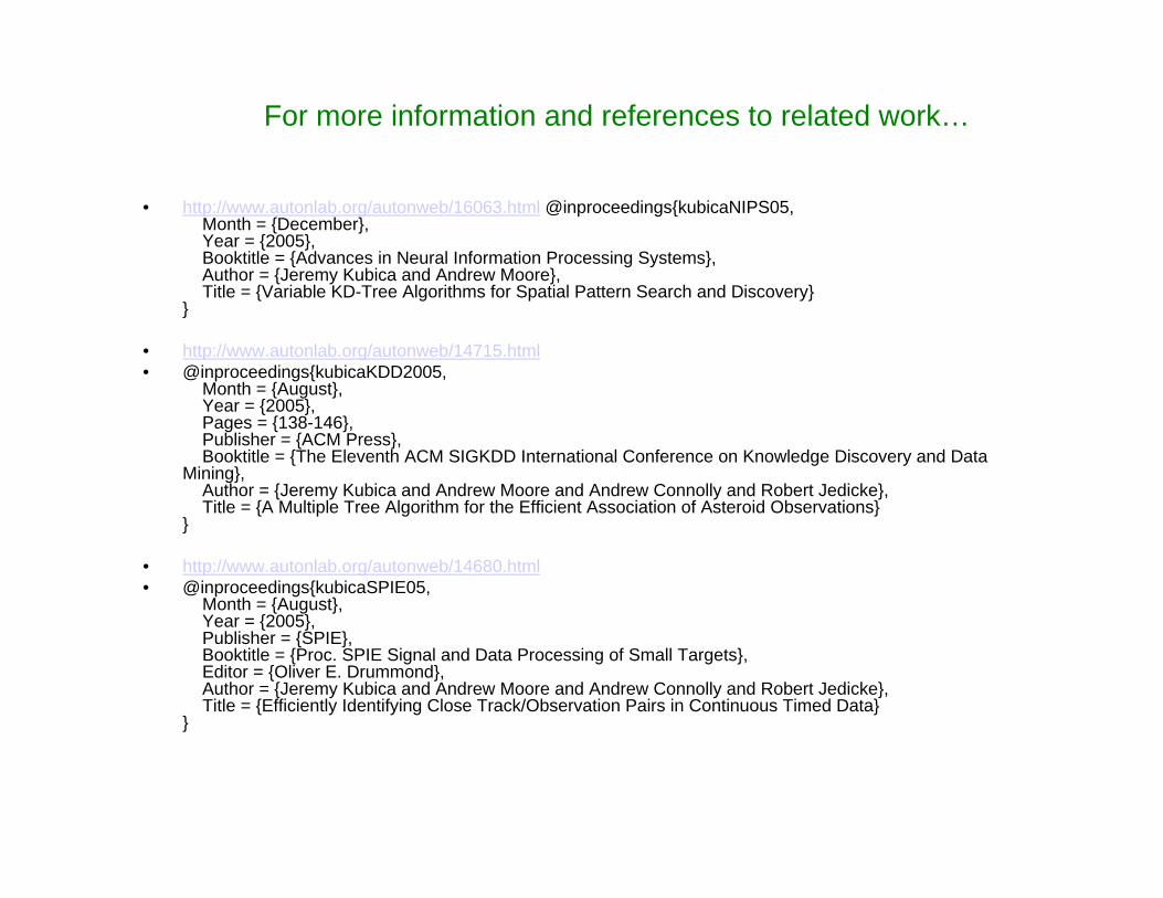
For more information and references to related work…
• http://www.autonlab.org/autonweb/14667.html@inproceedings{neill-rectangles,
Howpublished = {Conference on Knowledge Discovery in Databases (KDD) 2004},
Month = {August},Year = {2004},Editor = {J. Guerke and W. DuMouchel},Author = {Daniel Neill and Andrew Moore},Title = {Rapid Detection of Significant Spatial Clusters}
}
• http://www.autonlab.org/autonweb/15868.html@inproceedings{sabhnani-pharmacy,
Month = {August},Year = {2005},Booktitle = {Proceedings of the KDD 2005 Workshop on Data Mining Methods
for Anomaly Detection},Author = {Robin Sabhnani and Daniel Neill and Andrew Moore},Title = {Detecting Anomalous Patterns in Pharmacy Retail Data}
}
• Software: http://www.autonlab.org/autonweb/10474.html
For more information and references to related work…
• http://www.autonlab.org/autonweb/16063.html @inproceedings{kubicaNIPS05,Month = {December},Year = {2005},Booktitle = {Advances in Neural Information Processing Systems},Author = {Jeremy Kubica and Andrew Moore},Title = {Variable KD-Tree Algorithms for Spatial Pattern Search and Discovery}
}
• http://www.autonlab.org/autonweb/14715.html• @inproceedings{kubicaKDD2005,
Month = {August},Year = {2005},Pages = {138-146},Publisher = {ACM Press},Booktitle = {The Eleventh ACM SIGKDD International Conference on Knowledge Discovery and Data
Mining},Author = {Jeremy Kubica and Andrew Moore and Andrew Connolly and Robert Jedicke},Title = {A Multiple Tree Algorithm for the Efficient Association of Asteroid Observations}
}
• http://www.autonlab.org/autonweb/14680.html• @inproceedings{kubicaSPIE05,
Month = {August},Year = {2005},Publisher = {SPIE},Booktitle = {Proc. SPIE Signal and Data Processing of Small Targets},Editor = {Oliver E. Drummond},Author = {Jeremy Kubica and Andrew Moore and Andrew Connolly and Robert Jedicke},Title = {Efficiently Identifying Close Track/Observation Pairs in Continuous Timed Data}
}
Cached Sufficient StatisticsNew searches over cached statistics
Biosurveillance and EpidemiologyScan StatisticsCached Scan StatisticsBranch-and-Bound Scan StatisticsRetail data monitoringBrain monitoringEntering Google
AsteroidsMulti (and I mean multi) object target tracking Multiple-tree searchEntering Google

Justifiable Conclusions
Justifiable Conclusions• Geometry can help
tractability of Massive Statistical Data Analysis
• Cached sufficient statistics are one approach
• Not merely for simple friendly aggregates
Justifiable Conclusions• Geometry can help
tractability of Massive Statistical Data Analysis
• Cached sufficient statistics are one approach
• Not merely for simple friendly aggregates
Fluffy Conclusion“Theorem of Statistical
Computation Benevolence”
If Statistics thinks you’re going the right way, it will throw in computational opportunities for you
Papers, Software, Example Datasets, Tutorials: www.autonlab.org

For more information and references to related work…• http://www.autonlab.org/autonweb/14667.html@inproceedings{neill-rectangles,
Howpublished = {Conference on Knowledge Discovery in Databases (KDD) 2004},Month = {August}, Year = {2004},Editor = {J. Guerke and W. DuMouchel},Author = {Daniel Neill and Andrew Moore},Title = {Rapid Detection of Significant Spatial Clusters}
}
• http://www.autonlab.org/autonweb/15868.html@inproceedings{sabhnani-pharmacy,
Month = {August}, Year = {2005},Booktitle = {Proceedings of the KDD 2005 Workshop on Data Mining Methods for Anomaly Detection},Author = {Robin Sabhnani and Daniel Neill and Andrew Moore},Title = {Detecting Anomalous Patterns in Pharmacy Retail Data}
} • http://www.autonlab.org/autonweb/16063.html @inproceedings{kubicaNIPS05,
Month = {December}, Year = {2005},Booktitle = {Advances in Neural Information Processing Systems},Author = {Jeremy Kubica and Andrew Moore},Title = {Variable KD-Tree Algorithms for Spatial Pattern Search and Discovery}
}
• http://www.autonlab.org/autonweb/14715.html• @inproceedings{kubicaKDD2005,
Month = {August}, Year = {2005},Pages = {138-146},Publisher = {ACM Press},Booktitle = {The Eleventh ACM SIGKDD International Conference on Knowledge Discovery and Data Mining},Author = {Jeremy Kubica and Andrew Moore and Andrew Connolly and Robert Jedicke},Title = {A Multiple Tree Algorithm for the Efficient Association of Asteroid Observations}
}
• http://www.autonlab.org/autonweb/14680.html• @inproceedings{kubicaSPIE05,
Month = {August},Year = {2005}, Publisher = {SPIE},Booktitle = {Proc. SPIE Signal and Data Processing of Small Targets},Editor = {Oliver E. Drummond},Author = {Jeremy Kubica and Andrew Moore and Andrew Connolly and Robert Jedicke},Title = {Efficiently Identifying Close Track/Observation Pairs in Continuous Timed Data}
}
• Software: http://www.autonlab.org/autonweb/10474.html