New dynamic programming algorithms for the resource

New dynamic programming algorithms for the

resource-constrained elementary shortest path

problem

Giovanni Righini, Matteo Salani∗

Dipartimento di Tecnologie dell’InformazioneUniversita degli Studi di Milano

Via Bramante 65, 26013 Crema, Italy

January 2005

Abstract

The resource-constrained elementary shortest path problem arises asa pricing subproblem in branch-and-price algorithms for vehicle rout-ing problems with additional constraints. We address the optimizationof the resource-constrained elementary shortest path problem and wepresent and compare three methods. The first method is a well-knownexact dynamic programming algorithm improved by new ideas, such asbi-directional search with resource-based bounding. The second methodconsists of a branch-and-bound algorithm, where lower bounds are com-puted by dynamic programming with state space relaxation; we show howbounded bi-directional search can be combined with state space relaxationand we present different branching strategies and their hybridization. Thethird method, called decremental state space relaxation, is a new one; ex-act dynamic programming and state space relaxation are two special casesof this new method. The experimental comparison of the three methodsis definitely favourable to decremental state space relaxation. Computa-tional results are given for different kinds of resources, arising from thecapacitated vehicle routing problem, the vehicle routing problem with dis-tribution and collection and the vehicle routing problem with capacitiesand time windows.

Keywords: shortest path, vehicle routing, column generation, dynamic pro-gramming, branch-and-bound.

∗Corresponding author: ([email protected])

1

1 Introduction

Branch-and-price is one of the most effective techniques for the exact optimiza-tion of vehicle routing problems (VRP) with additional constraints. At eachnode of a branch-and-bound tree a relaxation of the set covering reformulationof the problem is solved via column generation. Algorithms based on this tech-nique can solve constrained VRP instances with more than 100 vertices (seefor instance Kohl et al. [20]). When vehicle routing problems with additionalconstraints are solved via column generation and branch-and-price, the pricingproblem requires to find a resource-constrained elementary path of minimumcost between two given vertices of a weighted graph, with positive costs on thearcs and non-negative prizes on the vertices. The cost of the path is given bythe sum of the costs of the arcs traversed minus the sum of the prizes collectedat the vertices visited. Exact optimization is needed to find new columns withnegative reduced cost or to prove that none of them exists. For a detailed ex-position of branch-and-price methods for vehicle routing problems we refer thereader to Desrosiers et al. [11], Bramel and Simchi-Levi [4] and Cordeau et al.[6].

If the underlying graph may have negative cost cycles (which is the case whenthere are prizes on the vertices), the resource-constrained elementary shortestpath problem (RCESPP) is strongly NP-hard: the proof is due to Dror [13].The most commonly used technique to solve the RCESPP to optimality is dy-namic programming, relying upon the seminal work by Desrochers [7] for theresource-constrained shortest path problem (RCSPP) in which the solution isnot required to be elementary. Other methods, based on Lagrangean relaxation,were proposed by Handler and Zang [17] and Beasley and Christofides [3] andwere recently examined by Dumitrescu and Boland [14], who devised improvedpreprocessing and bounding techniques. However these methods require a graphfree from negative cost cycles, so that the Lagrangean subproblem is a polyno-mially solvable shortest path problem. The case with negative cost cycles wasconsidered by Feillet et al. [15], who suggested some improvements to the basicDesrochers’ algorithm [7]. For a recent survey on models and algorithms for theRCSPP and the RCESPP we refer the reader to Irnich and Desaulniers [18].

In this paper we consider the problem of computing optimal solutions to theRCESPP, as in Feillet et al. [15], and we present three different approaches: ex-act dynamic programming, branch-and-bound based on state space relaxationand decremental state space relaxation. All of them use dynamic programmingbut in different ways: in the first case an exact dynamic programming algo-rithm computes the optimal solution of the RCESPP; this approach was takenfor instance by Feillet et al. [15] and Righini and Salani [22]. In the secondcase a dynamic programming algorithm with state space relaxation is used tooptimize the RCSPP, where cycles are allowed. This gives lower bounds cor-responding to non-elementary paths and these lower bounds are exploited ina branch-and-bound framework. The third method, decremental state spacerelaxation, is original and includes both exact dynamic programming and statespace relaxation as special cases.

2

The performance of exact dynamic programming algorithms for the RCESPPcan be significantly improved through bi-directional search and resource-basedbounding, as shown by Righini and Salani [22]. In this paper we review them andwe show that they can be applied also to dynamic programming with state spacerelaxation and decremental state space relaxation. We report on the outcome ofexperimental comparisons between these methods when solving RCESPPs withdifferent kinds of resource constraints. In particular we consider three variationsof the RCESPP arising from three well-known vehicle routing problems withadditional constraints, namely the capacitated vehicle routing problem (CVRP),the vehicle routing problem with distribution and collection (VRPDC) and thevehicle routing problem with capacities and time windows (CVRPTW).

The outline of this paper is the following: in Section 2 we formally definethe RCESPP; in Section 3 we review the dynamic programming algorithms forits exact optimization; in Section 4 we review bounded bi-directional dynamicprogramming; in Section 5 we analyze state space relaxation to compute lowerbounds; in Section 6 we present the branch-and-bound algorithm; in Section7 we introduce decremental state space relaxation; in Section 8 we report oncomputational results; in Section 9 we point out some conclusions. The contentof Sections 3 and 4 is a review of concepts already described in [22], which havebeen recalled here in order to make this paper self-contained.

2 Problem definition

The RCESPP is defined as follows: a graph G(V,A) is given, where the vertexset V is made by a set of vertices N representing N customers and two vertices sand t representing the depot. A non-negative cost cij is associated with each arc(i, j) ∈ A; arc costs correspond to shortest paths and therefore they satisfy thetriangle inequality. A non-negative prize λi is associated with each vertex i ∈ N ,a non-negative cost λ0 is associated with the depot. A vehicle must go from s tot, visiting a subset of the other vertices; no cycles are allowed. The objective isto minimize the cost, given by the sum of the costs of the arcs traversed minusthe sum of the prizes collected at the vertices visited. In a column generationframework this corresponds to generate columns of minimum reduced cost forthe linear relaxation of the set covering reformulation of a VRP: λi is the dualmultiplier associated with the covering constraint of vertex i and λ0 is the dualmultiplier asociated with the constraint on the maximum number of availablevehicles.

These definitions of the problem are common to all RCESPP versions arisingfrom the different routing problems we consider. Additional constraints, thatdepend on the kind of vehicle routing problem at hand, are modeled as resourceconstraints and they are specified hereafter.

Capacity. In the CVRP a non-negative integer demand di is associatedwith each vertex i ∈ N and a positive integer vehicle capacity Q is given. Thesum of the demands of the nodes visited by the same vehicle cannot exceed Q.

3

Distribution and collection. In the VRPDC each vertex i has two non-negative integer quantities pi and di associated with it, representing respectivelythe amount of load to be collected and to be delivered at that vertex. Each ve-hicle has a positive integer capacity Q, it leaves the depot carrying the totalamount of load it must deliver and returns to the depot carrying the totalamount of load it has collected. The capacity cannot be exceeded anywherealong the path.

Capacity and time windows. In the CVRPTW a non-negative integerservice time θi and a time window [ai, bi], defined by two non-negative integers,are associated with each vertex i ∈ N and the service at each visited vertexmust start inside its time window. If the vehicle arrives at vertex i before timeai, it waits until ai. The traveling time from any vertex i to any vertex j is anon-negative integer datum vij .

We chose these three problems, because they offer a significant mix of differ-ent characteristics. In the CVRP there is only one resource, whose consumptiondepends on the vertices visited. In the VRPDC there are two resources associ-ated with the vertices visited and they are interacting: the consumption of one ofthem also depends on the consumption of the other. In the CVRPTW there aretwo resources, one associated with the vertices visited and the other associatedwith the arcs traversed. In all cases resources are subject to a global constrainton their overall consumption along the s-t path, with the exception of the casewith time windows, where a resource (time) is subject to local constraints, onefor each vertex visited.

3 Exact dynamic programming

The starting point for our exposition is the reaching algorithm of Desrochers [7]for the RCSPP, that is an extension of the well-known shortest path algorithmof Ford and Bellman (see [2]). The algorithm assigns states to each vertex: eachstate associated with vertex i represents a path from s to i. Each state includesa resource consumption vector R whose component Rr represents the quantityof resource r used along the corresponding path. Each state has an associatedcost C and the optimal solution corresponds to a minimum cost state associatedwith vertex t. The algorithm repeatedly extends each state to generate newstates. The extension of a state corresponds to appending an additional arc(i, j) to a path from s to i, obtaining a path from s to j. This operation isrepeated until all states have been extended in all feasible ways. This dynamicprogramming algorithm, devised for the RCSPP, can be adapted to solve theRCESPP on graphs with negative cost cycles. To this purpose Beasley andChristofides [3] proposed to add to the state an additional binary resource foreach vertex i ∈ N ; there is only one unit available for each dummy resource andit is consumed when the correponding vertex is visited. The consumption of

4

the N dummy resources is indicated by a vector S initialized at 0. Note that Sdoes not keep any information about the order in which the vertices are visited.Hence in the basic exact dynamic programming algorithm for the RCESPP eachstate is represented by a label of the form (S, R,C, i).

When a label (S,R, C, i) associated with vertex i is extended to generateanother feasible label (S′, R′, C ′, j) associated with vertex j, the resource con-sumption vectors and the cost are updated and the new state is checked forfeasibility, as follows.

Cost. The cost is inizialized at 0 at vertex s and it is updated according tothe formula

C ′ = C − λi/2 + cij − λj/2 (1)

where λi = −λ0 if i = s and λj = −λ0 if j = t.

Dummy resources. The dummy resources vector S is initialized at 0 atvertex s and the update rule is:

S′k ={

Sk + 1 k = jSk k 6= j

A state (S, R,C, i) corresponds to an elementary path only if Sk ≤ 1 ∀k ∈ N .

According to the different kind of resources considered the extension rulesand the feasibility test on R take different forms.

Capacity. The capacity constraint is modeled by a single resource, rep-resenting the amount of capacity still available along the path. Let q be theamount of resource consumed. When a vehicle leaves vertex s all the resourceis available, that is q = 0. Every time a vertex is visited, q is increased by thedemand of that vertex. Hence the extension rule is:

q′ = q + dj (2)

A state (S, q, C, i) is feasible only if q ≤ Q.

Distribution and collection. In this case the capacity constraint is takeninto account by two additional resources, whose consumption is indicated byπ and δ. The first resource at vertex i is the amount of load that the vehiclecan pick-up after visiting i. Its consumption π increases after every pick-upoperation, because when the vehicle visits vertex i, it consumes pi units of thisresource. The second resource at vertex i indicates the amount of load thatthe vehicle can deliver after visiting i. This quantity is equal to the differencebetween the capacity Q and the maximum amount of load that has been onboard of the vehicle since its departure from s up to i. Initially Q units areavailable for the second resource and the available resource decreases each time a

5

delivery operation is performed but it may decrease also after pick-up operations:the maximum amount the vehicle can deliver after visiting i cannot be greaterthan the maximum amount it can pick-up after visiting i. Hence both π and δare initialized at 0 and the extension rule is:

π′ = π + pj

δ′ = max{δ + dj , π + pj}

A state (S, π, δ, C, i) is feasible only if π ≤ Q and δ ≤ Q. Note that for thedefinition of π and δ the latter condition implies the former.

Capacity and time windows. In this case the time elapsed is a consumedresource, monotonically increasing along the path. To represent the capacityconstraint and the time window constraints, we need two resources, whose con-sumption is respectively indicated by q and τ : they are the capacity and thetime consumed up to the beginning of service at each vertex. Both of them areinitialized at 0 and the extension rules are:

q′ = q + dj

τ ′ = max{τ + θi + vij , aj}

A state (S, q, τ, C, i) is feasible only if q ≤ Q and τ ≤ bi.

The effectiveness of the dynamic programming algorithm heavily depends onthe number of states generated. Hence it is essential to fathom feasible stateswhich cannot lead to the optimal solution. To this purpose suitable dominancetests are always performed when states are extended, so that the algorithmrecords only non-dominated states. The dominance test is the following. Let(S′, R′, C ′, i) and (S′′, R′′, C ′′, i) be the labels of two states associated with ver-tex i; then (S′, R′, C ′, i) dominates (S′′, R′′, C ′′, i) only if

S′ ≤ S′′

R′ ≤ R′′

C ′ ≤ C ′′

and at least one of the inequalities is strict.When the consumption of some resource is non-negative and obeys the tri-

angle inequality, the domination rule can be made stronger, as pointed out byFeillet et al. [15]. The idea is to identify vertices which cannot be visited in anyfeasible extension of a given state owing to the limits on the resources. Thesevertices are called unreachable. When a vertex is found to be unreacheable froma given state, the consumption of the corresponding dummy resource in thatstate can be set to 1, as if the vertex had already been visited. This allowsthe dynamic programming algorithm to identify a larger number of dominatedstates and to fathom them, thus reducing the computation time. We incorpo-rated this method in all the algorithms we considered: the triangle inequality

6

is certainly satisfied by the resources whose consumption occurs at the vertices,such as the RCESPP with capacity and the RCESPP with distribution andcollection. The applicability to the case with time windows, where resource τis consumed on the arcs, depends on whether the traveling times satisfy thetriangle inequality or not; to apply the techniques of Feillet et al. to the timeresource, we assumed vij = cij ∀(i, j) ∈ A in our tests.

The order in which the states are extended may be very important for theeffectiveness of the overall algorithm. Here we consider label-correcting algo-rithms like those of Desrosiers et al. [12] and Feillet et al. [15]. States areexplored according to the vertices they are associated with. All vertices arecyclically visited and for each vertex the algorithm extends all states that havenot yet been extended. States associated with the same vertex can be sortedaccording to a secondary criterion, for instance according to the cost or theconsumption of a certain resource. In the three cases we have considered statesassociated with the same vertex are sorted according to the values of q, π andτ respectively.

Label-setting algorithms have also been proposed (see for instance Desrochersand Soumis [9]) but they require an hypothesis stronger than resource consump-tion monotonicity: in particular there must exists a resource whose consumptionis not less than a certain known amount β at each extension. In this case it ispossible to define buckets of size β and to mark as permanent all those labelsfor which the resource consumption falls in the range of the first bucket not yetextended. For a more detailed exposition of label-setting algorithms we referthe reader to Desrosiers et al. [11].

4 Bounded bi-directional dynamic programming

Bounded bi-directional dynamic programming has been recently introduced byRighini and Salani [22] to improve the exact dynamic programming algorithmdescribed above. In bi-directional dynamic programming states are extendedboth forward from vertex s to its successors and backward from vertex t to itspredecessors (see for instance Mingozzi et al. [21] for an application of this ideato a constrained TSP). With each vertex i ∈ V we associate forward states indi-cated by (Sfw, Rfw, Cfw, i) and backward states indicated by (Sbw, Rbw, Cbw, i).A path from s to t is detected each time a forward state (Sfw, Rfw, Cfw, i) and abackward state (Sbw, Rbw, Cbw, j) can be feasibly joined. Hereafter we describebackward extension rules and feasibility tests for backward states. Dominancetests on backward states are identical to those for forward states. We also illus-trate the operation of joining forward and backward states to produce s-t pathsand we review the idea of resource-based bounding.

4.1 Backward extension and feasibility tests

The backward cost Cbw is initialized at 0 at vertex t and whenever a backwardstate (Sbw, Rbw, Cbw, j) is extended to a backward state (S

′bw, R′bw, C

′bw, i) the

7

cost is updated according to the formula:

C′bw = Cbw − λi/2 + cij − λj/2

where λi = −λ0 if i = s and λj = −λ0 if j = t.The dummy resources vector Sbw is initialized at 0 at vertex t and the

extension rule is:

S′bwk =

{Sbw

k + 1 k = jSbw

k k 6= j

A backward path is feasible only if Sbwk ≤ 1 ∀k ∈ N .

Capacity. Resource consumption qbw in a backward state associated withvertex j represents the overall demand of customers visited from j (included)to t. The consumption qbw is initialized at 0 at vertex t. When a feasiblebackward path is extended along arc (i, j) from a state (Sbw, qbw, Cbw, j) to astate (S′bw, q′bw, C ′bw, i), the extension rule is:

q′bw = qbw + di (3)

A backward path is feasible only if qbw ≤ Q.

Distribution and collection. Two resources, whose consumption is indi-cated by πbw and δbw, are associated with each backward state. Their meaning,initialization and extension rules are symmetrical to those of forward labels: δbw

indicates the amount of load delivered between j and t and πbw indicates themaximum overall amount of load on board of the vehicle between j and t. Whena backward path is extended along arc (i, j) from a state (Sbw, πbw, δbw, Cbw, j)to a state (S′bw, π′bw, δ′bw, C ′bw, i), the extension rule is:

π′bw = max{δbw + di, πbw + pi}

δ′bw = δbw + di

A backward path is feasible only if πbw ≤ Q and δbw ≤ Q (the former conditionimplies the latter).

Capacity and time windows. In the case of time windows for the sake ofsymmetry it is useful to define forward and backward time windows [afw

i , bfwi ]

and [abwi , bbw

i ] as follows:

afwi = ai

bfwi = bi

abwi = ai + θi

bbwi = bi + θi

8

The forward time window represents the range of feasible arrival times at vertexi, while the backward time window represents the range of feasible departuretimes from vertex i. The overall resource availability T is equal to the maximumfeasible arrival time at vertex t that is T = maxi∈N∪{s}{bfw

i + θi + vit}. Theresource consumption τ bw in a backward state associated with vertex j repre-sents the minimum time which must be consumed since the departure from jup to the arrival at t. When a feasible backward path is extended along arc(i, j) from a state (Sbw, qbw, τ bw, Cbw, j) to a state (S′bw, q′bw, τ ′bw, C ′bw, i), theextension rules are:

q′bw = qbw + di

τ ′bw = max{τ bw + θj + vij , T − bbwi }

A backward label associated with vertex j is feasible only if qbw ≤ Q andτ bw ≤ T − abw

j .

4.2 Joining forward and backward states

Forward and backward paths must be joined together to produce complete s-tpaths. When a forward path (Sfw, qfw, Cfw, i) is joined with a backward path(Sbw, qbw, Cbw, j) the cost of the resulting s-t path is equal to

Cfw − λi/2 + cij − λj/2 + Cbw

The join is subject to certain feasibility conditions on the resources. In particularthe feasibility test on dummy resources S imposes that a same vertex can notbe visited by both paths.

Sfwk + Sbw

k ≤ 1 ∀k ∈ N

The feasibility test on problem-dependent resources R imposes that for eachresource the consumption in the overall s-t path can not exceed the overallamount of available resource. Hereafter we define the feasibility tests for eachspecific kind of resource constraints considered.

Capacity. The feasibility test on the capacity for joining a forward path(Sfw, qfw, Cfw, i) with a backward path (Sbw, qbw, Cbw, j) is

qfw + qbw ≤ Q

Distribution and collection. The feasibility conditions to join a forwardpath (Sfw, πfw, δfw, Cfw, i) with a backward path (Sbw, πbw, δbw, Cbw, j) are:

πfw + πbw ≤ Q

δfw + δbw ≤ Q

9

Capacity and time windows. The feasibility conditions to join a forwardpath (Sfw, qfw, τfw, Cfw, i) with a backward path (Sbw, qbw, τ bw, Cbw, j) are:

qfw + qbw ≤ Q

τfw + θi + vij + θj + τ bw ≤ T

4.3 Resource-based bounding

Since all forward and backward states generated by the bi-directional searchalgorithm are tentatively joined, it is crucial to reduce their number as muchas possible. To this purpose we select a critical resource, whose consumptionis monotone along the paths, and we do not extend states in which at leasthalf of the available amount of that resource has been consumed. This allowsto greatly reduce the number of states generated still guaranteeing that theoptimal solution will be found. Hereafter we describe how we have chosen thecritical resource for each different kind of problem.

Capacity. The critical resource in this case is capacity. Forward and back-ward states are extended only if their associated resource consumption value,qfw or qbw respectively, is less than Q/2.

Distribution and collection. In this case there are two resources; we con-sider as a critical resource the sum of the resource consumptions ρfw = πfw+δfw

for forward states and ρbw = πbw + δbw for backward states and in both direc-tions we extend only those states for which ρ < Q.

Capacity and time windows. In this last case we consider time as thecritical resource and we extend only forward states for which τfw < T/2 andbackward states for which τ bw < T/2.

The combination of bi-directional search with resource-based bounding al-lows to solve larger instances (or the same instances in less time) than mono-directional dynamic programming; detailed experimental results are reported in[22]. In the next section we show how bi-directional search and resource-basedbounding can be incorporated into dynamic programming algorithms based onstate space relaxation.

We report hereafter the pseudo-code of the bounded bi-directional algorithm.We use the following symbols: Γfw

i and Γbwi are the lists of forward and back-

ward states associated with vertex i; ∆+i and ∆−

i are the sets of successors andpredecessors of vertex i; E is the set of vertices to be examined; Extendfw(l, k)and Extendbw(l, k) are respectively the forward and backward extension proce-dures, that extend state l to vertex k; they check the resource constraints andproduce only feasible states; EFF (Γ, l) is the procedure which inserts state linto set Γ applying the domination rules; Feasible(li, lj) checks the resourcecompatibility of forward state li and backward state lj according to problem-

10

dependent rules; Save(li, lj) saves the solution obtained joining the two statesli and lj ;

Algorithm 1 RCESPP - Bi-directional dynamic programming// Initialization //Γfw

s ← {(0,0, 0, s)}Γbw

t ← {(0,0, 0, t)}for all i ∈ V \ {s} do Γfw

i ← ∅for all i ∈ V \ {t} do Γbw

i ← ∅E ← {s, t}// Search //repeat

// Vertex selection //Select i ∈ E// Forward extension //for all li = (Si, Ri, Ci, i) ∈ Γfw

i dofor all j ∈ ∆+

i such that Sij = 0 do

lj ← Extendfw(li, j)Γfw

j ← EFF (Γfwj , lj)

if Γfwj has changed then E ← E ∪ {j}

// Backward extension //for all li = (Si, Ri, Ci, i) ∈ Γbw

i dofor all k ∈ ∆−

i such that Sik = 0 do

lk ← Extendbw(li, k)Γbw

k ← EFF (Γbwk , lk)

if Γbwk has changed then E ← E ∪ {k}

E ← E \ {i}until E = ∅// Join between forward and backward paths //for all i ∈ V

for all li = (Si, T i, Ci, i) ∈ Γfwi

for all j ∈ Vfor all lj = (Sj , T j , Cj , j) ∈ Γbw

j

if Feasible(li, lj) then Save(li, lj)

5 State space relaxation

State space relaxation was introduced by Christofides et al. [5] in 1981. Thestate space S explored by the dynamic programming algorithm is projected ontoa lower dimensional space T so that each state in T retains the minimum costamong those of its corresponding states in S (assuming the objective functionmust be minimized). In this way the number of states to be explored is dras-

11

tically reduced; the drawback is that some original state corresponding to aninfeasible solution in S may be projected onto a state corresponding to a fea-sible solution in T and therefore the search in the relaxed state space does notguarantee to find an optimal solution but rather a lower bound.

State space relaxation has been used as a method alternative to exact op-timization of the pricing problem in branch-and-price algorithms for the VRPwith additional constraints (see for instance Desrochers et al. [8]): instead ofthe optimal value of the pricing problem, a lower bound is obtained. This al-lows faster convergence of the column generation algorithm at the expense ofa weaker lower bound. Columns containing cycles must be eliminated throughbranching. Here on the contrary we focus on the use of state space relaxation forthe exact optimization of the pricing problem by a branch-and-bound algorithm.

Our state space relaxation consists of mapping each state (S,R, C, i) ontoa new state (σ,R, C, i), where σ =

∑Nk=1 Sk represents the length of the path,

that is the number of vertices visited (excluding s). Since each component of theresource consumption vector R may take on a finite number of values and σ canvary between 0 and N , a dynamic programming algorithm based on state spacerelaxation must explore only a pseudo-polynomial number of states. From theviewpoint of complexity and computing time this makes a big difference withrespect to the exact dynamic programming algorithm in which vector S yieldsan exponential number of possible states. The surrogate resource consumptionσ is initialized as 0 and it is increased by one unit each time a state is extended.Since the state does no longer keep information about the set of already visitedvertices, cycles are no longer forbidden; therefore the path is guaranteed to befeasible with respect to the resource constraints but it is not guaranteed to beelementary.

In the state space relaxation algorithm the domination rule is modified asfollows: a state (σ′, R′, C ′, i) dominates a state (σ′′, R′′, C ′′, i) only if

σ′ ≤ σ′′

R′ ≤ R′′

C ′ ≤ C ′′

and at least one of the inequalities is strict.This state space relaxation of the RCESPP into the RCSPP can be tight-

ened by eliminating all cycles of length two. This is easily accomplished by aduplication of the labels (see for instance Desrochers et al. [8]). Irnich andVilleneuve [19] proposed a method to eliminate cycles of length k ≥ 3, but thecomputational complexity of their method dramatically increases with k. Hencewe incorporated in our algorithms the technique to avoid cycles of length two.

The definitions above apply to both forward and backward states when bi-directional search is employed. In such case σfw and σbw represent respectivelythe number of forward extensions from s and the number of backward extensionsfrom t. We bound bi-directional search in the same way described above, thatis on the basis of the value of a critical resource.

When bounded bi-directional search is coupled with state space relaxationthe join of forward and backward paths becomes critical: both the forward path

12

and the backward path to be joined may contain cycles; moreover a cycle canbe produced by the join, even if the two paths are elementary. These two casesare illustrated in figure 1. In addition there may be many different ways to joinforward and backward paths providing the same solution. The former issue isaddressed in the next section, where branching strategies are illustrated; thelatter is addressed hereafter.

gs g gi gj g gt

g g g g

- - - - -

¾ ¾

¢¢¢A

AAU ¢¢¢A

AAU gs g g- -

gj gi¾

¢¢¢A

AAUg g gt- -

Figure 1: On the left: an s-t path made of non-elementary paths s-i and j-t.On the right: a non-elementary s-t path made of elementary paths s-i and j-t.

5.1 Paths join and solutions uniqueness

The bounded bi-directional dynamic programming algorithm can provide du-plicate solutions: consider for instance an s-t path including vertices i, j and kin this order. If the constraint on the critical resource is not tight, it is possi-ble that forward states for vertices i and j and backward states for vertices jand k are generated. Therefore the same s-t path can be obtained by joining aforward state of i with a backward state of j as well as joining a forward stateof j with a backward state of k. This unpleasant phenomenon can be avoidedwith an additional test: we accept an s-t path only when it is produced bythe join of a forward state and a backward state, for which the forward andbackward consumptions of the critical resource are as close as possible to halfthe overall consumption for that s-t path, that is the two states are as close aspossible to the “half way point” along the s-t path. Let rfw and rbw be the crit-ical resource consumptions in forward and backward paths. Among all possiblepairs of forward and backward states producing the same s-t path we choosethe one for which φ = |rfw − rbw| is minimum. The test is done in constanttime for each candidate pair of states, since the position closest to the “half-waypoint” is detected by direct comparison with the next position along the pathif rfw < rbw and with the previous position if rfw > rbw. In case of tie betweentwo positions for which φ is minimum, we choose the one with rfw > rbw. Thistest guarantees that each s-t path is generated only once.

We report hereafter the pseudo-code of the state space relaxation algorithmwhere the terminology used is the same as before. In the joining step theprocedure HalfWay(li, lj) checks if the s-t path obtainable joining the twostates li and lj satisfies the “half-way-point” conditions.

13

Algorithm 2 RCSPP - Bi-directional state space relaxation// Initialization //Γfw

s ← {(0,0, 0, s)}Γbw




// Vertex selection //Select i ∈ E// Forward extension //for all li = (σi, Ri, Ci, i) ∈ Γfw

i dofor all j ∈ ∆+

i dolj ← Extendfw(li, j)Γfw



// Backward extension //for all li = (σi, Ri, Ci, i) ∈ Γbw

i dofor all k ∈ ∆−

i dolk ← Extendbw(li, k)Γbw




for all li = (σi, T i, Ci, i) ∈ Γfwi

for all j ∈ Vfor all lj = (σj , T j , Cj , j) ∈ Γbw

j

if Feasible(li, lj) and HalfWay(li, lj)then Save(li, lj)

6 Branch-and-bound

In this section we describe a branch-and-bound algorithm which solves the RCE-SPP to optimality, exploiting the RCSPP lower bound given by the boundedbi-directional dynamic programming algorithm with state space relaxation. InSubsection 6.1 we describe the branching policies needed to eliminate cycles:every time the optimal solution of the RCSPP is not elementary, the currentnode of the search tree is replaced by children nodes in which some additionalconstraints are added to the RCSPP.

14

Search policy. The search policy we use to explore the branch-and-boundtree is best-first, that is the open nodes of the tree are ranked according to thevalue of their associated lower bound and the most promising node is exploredfirst.

Upper bounding. At each node of the branch-and-bound tree and at eachiteration of the column generation algorithm a feasible solution is computedwith a nearest neighbor heuristic. Starting from the depot s the most convenientvertex among the feasible ones is chosen until the path reaches t. For a vertex tobe feasible we check that no resource constraint is exceeded and the vertex havenot been visited yet. At each vertex i the algorithm chooses the next feasiblevertex j such that j = argmink{cik − λk}.

6.1 Branching strategies

We present three different ways to perform branching, namely branching on cy-cles, branching on arcs and branching on resources. Our algorithm uses hybridbranching strategies in which all these techniques are exploited.

Branching on cycles. First we determine the minimum length cycle in theoptimal RCSPP solution. Then k children nodes are generated, where k is thelength of the cycle, that is the number of arcs traversed between two visits tothe same vertex: at child node h = 0, . . . , k−1 we fix the first h arcs of the cycleand we forbid the h + 1-th arc. We experimentally observed that, forbiddingcycles of length 2, k was very often equal to 3.

Branching on arcs. This binary branching scheme consists of selecting avertex entered or left by more than one arc in the RCSPP solution. Let (i1, j)and (i2, j) be two arcs entering vertex j in the RCSPP solution. Then we parti-tion the arcs entering j into two subsets I1 and I2 such that i1 ∈ I1 and i2 ∈ I2

and we forbid all arcs in I1 in one child node and all arcs in I2 in the other.

Branching on resources. When the optimal solution of the RCSPP hasa cycle, there exists at least one vertex ı that is visited more than once. Thebranching strategy consists of adding a constraint on the quantity of critical re-source consumed up to the visit of vertex ı. This idea was proposed by Gelinaset al. [16] for routing problems with time windows and it can be adapted to anyproblem with a critical resource whose consumption r is strictly monotone alongthe path. Given a branching vertex ı, let r′ and r′′ the two values of resourceconsumption in two states associated with ı with r′ < r′′. Then an integer valuer is chosen such that r′ < r ≤ r′′. Two children nodes are generated imposingthat the value of r at vertex ı satisfies r ≥ r in one child node and r ≤ r − 1 inthe other.

It is remarkable that the dynamic programming algorithm that computesthe lower bound can easily take into account the constraints imposed by all

15

branching techniques. In particular when arc (i, j) is forbidden, it is simplydeleted from the graph. The consequence of branching on the critical resourceis that each vertex has an associated window [ar, br] of feasible values for thecritical resource; when a path reaches that vertex with a critical resource con-sumption less than ar, the consumption is set to ar; when it reaches the vertexwith a critical resource consumption greater than br, it is declared infeasibleand it is discarded. This rule can be applied to both forward and backwardstates, with different resource windows for constraining forward and backwardconsumptions.

Hybrid branching. We obtained the best results when we employed hybridbranching strategies in our branch-and-bound algorithm. If either the forwardpath or the backward path forming the optimal RCSPP solution contain a cycle,we branch on the critical resource: we choose for branching the first vertexvisited more than once which is encountered moving along the forward (resp.backward) path from s to t (resp. from t to s); we consider r′ and r′′ as theresource consumptions at the first (resp. last) two visits of the branching vertexand we choose r = d r′+r′′

2 e. If the forward and the backward paths are bothelementary but a cycle is generated by their join, we branch on arcs or cycles.When we branch on arcs, the branching vertex is the first vertex visited morethan once which is encountered when moving along the path from the half waypoint forward.

We could not observe a clear domination between the hybrid branchingstrategies on resource/arcs and resource/cycles. In Section 8 we report on com-putational results obtained with each of them.

7 Decremental state space relaxation

The exact dynamic programming algorithm forbids multiple visits for each ver-tex, while the algorithm with state space relaxation does not. We pursued acompromise between these two extreme cases by the following idea: some ver-tices are identified as critical, according to the structure of the optimal RCSPPsolution obtained with state space relaxation. Let Θ indicate the set of criti-cal vertices at the current iteration. In the subsequent iteration the dynamicprogramming algorithm prevents multiple visits the vertices in Θ, still allowingmultiple visits to the others. This is easily accomplished by extending the statespace relaxation labels with a binary vector SΘ playing the same role as S inexact dynamic programming. The size of SΘ is however restricted only to thecritical vertices. When SΘ contains all the vertices the algorithm is equivalentto exact dynamic programming; when SΘ is empty it is equivalent to the al-gorithm with state space relaxation. Therefore we indicate this algorithm bydecremental state space relaxation (DSSR). The algorithm is run iteratively:every time it produces an optimal solution with cycles, the vertices visited morethan once are marked as critical and the algorithm restarts. Let Ψ the set ofvertices visited more than once in the optimal solution computed by the DSSR

16

algorithm. If Ψ is not empty, then another iteration is performed with a setof critical vertices equal to Θ′ = Θ ∪ Ψ. Hence the set of critical vertices isenlarged at each iteration and eventually the algorithm provides the optimalsolution to the RCESPP without having recourse to branching. We reporthereafter the pseudo-code of the decremental state space relaxation algorithm.where SΘ is the vector of dummy resources associated to the critical vertices;procedure MultipleV isits returns the set Ψ of vertices visited more than oncein the current optimal path.

8 Experimental results

For our experiments we used the same instances as in Feillet et al. [15] and Righ-ini and Salani [22]; they are derived from the well-known Solomon’s VRPTWbenchmark. For each kind of RCESPP problem we tested our algorithms ontwo classes of instances obtained from Solomon’s instances by considering thefirst 50 and 100 nodes. These datasets are divided into random, clustered andrandom-clustered categories, according to the displacement of the customers.Instances belonging to the same dataset have the customers located in the sameway and with the same delivery requests; these instances differ only for the timewindows.

When solving the RCESPP with capacities we considered one instance takenfrom each one of the three Solomon’s testsets (namely c101, r101 and rc101);we kept the original customer locations and delivery requests and we neglectedthe time windows. Then we derived from each original instance ten RCESPPinstances with 50 nodes and ten RCESPP instances with 100 nodes, by choosingten different values for the vehicle capacity from 10 to 100.

For the RCESPP with distribution and collection we kept the original de-livery requests and we derived the pickup requests as follows: pi = b0.8dic if iis odd and pi = b1.2dic if i is even. We generated ten instances with 50 nodesand ten instances with 100 nodes as before.

Finally, for the RCESPP with capacities and time windows we consideredthe original instances of Solomon’s dataset. In addition we also defined anotherdataset built on the difficult Solomon’s instance c 104; for each vertex i we keptthe original starting time of the time window, ai, and we set the end time asfollows: bi = ai + (1 + γ)θi for γ = 0.25 ∗ k and k = 0, . . . , 24, where θi is thegiven service time at vertex i.

For each set of instances we generated the prizes λi as random integer vari-ables uniformly distributed in [0, . . . , 20]; we set λ0 = 0. This data generationtechnique was devised by Feillet et al. [15] to have a reasonable number of neg-ative cycles. We rounded up all the Euclidean distances between customers tointeger values.

All tests were performed on a PC equipped with a PentiumIV 1.6GHz proces-sor with 512Mb RAM. The algorithms were coded in ANSI-C and compiled withgcc 3.0.4.

17

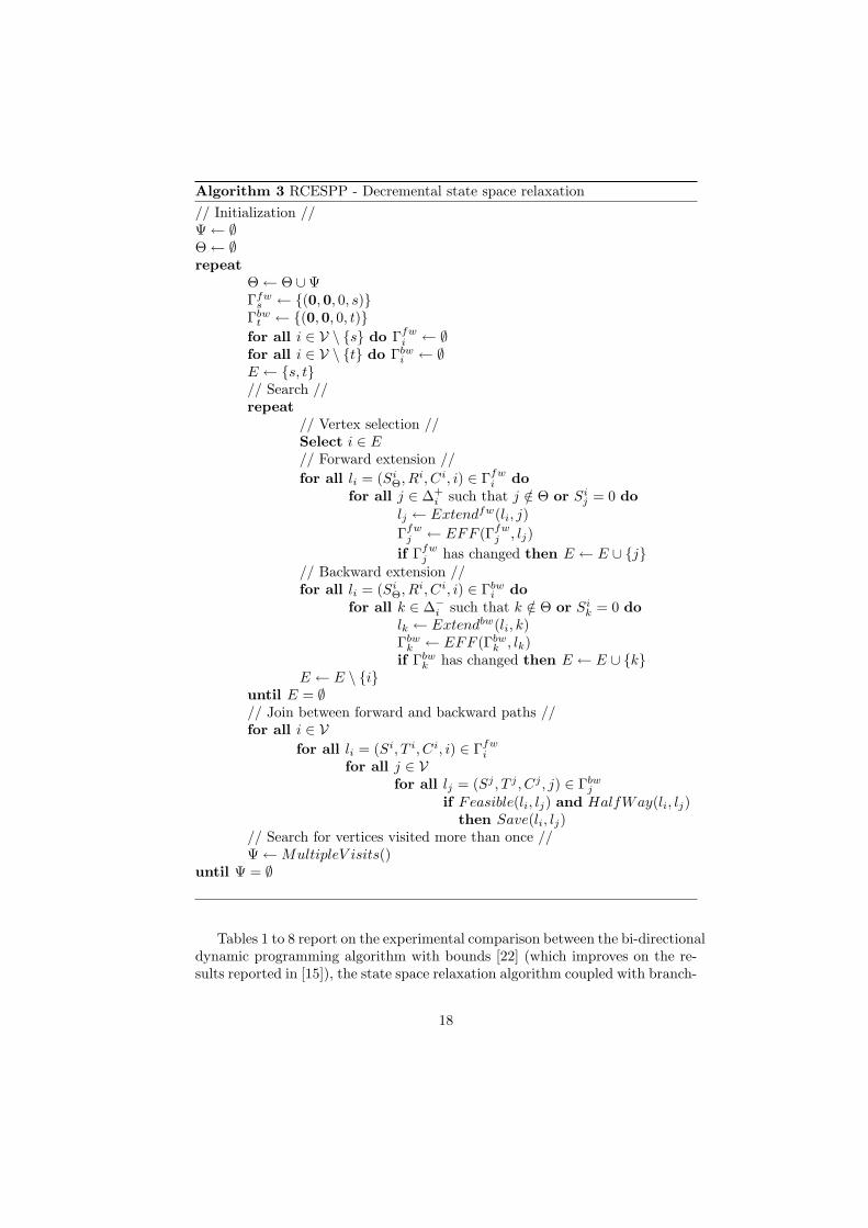
Algorithm 3 RCESPP - Decremental state space relaxation// Initialization //Ψ ← ∅Θ ← ∅repeat

Θ ← Θ ∪ΨΓfw

s ← {(0,0, 0, s)}Γbw




// Vertex selection //Select i ∈ E// Forward extension //for all li = (Si

Θ, Ri, Ci, i) ∈ Γfwi do

for all j ∈ ∆+i such that j /∈ Θ or Si

j = 0 dolj ← Extendfw(li, j)Γfw



// Backward extension //for all li = (Si

Θ, Ri, Ci, i) ∈ Γbwi do

for all k ∈ ∆−i such that k /∈ Θ or Si

k = 0 dolk ← Extendbw(li, k)Γbw




for all li = (Si, T i, Ci, i) ∈ Γfwi

for all j ∈ Vfor all lj = (Sj , T j , Cj , j) ∈ Γbw

j

if Feasible(li, lj) and HalfWay(li, lj)then Save(li, lj)

// Search for vertices visited more than once //Ψ ← MultipleV isits()

until Ψ = ∅

Tables 1 to 8 report on the experimental comparison between the bi-directionaldynamic programming algorithm with bounds [22] (which improves on the re-sults reported in [15]), the state space relaxation algorithm coupled with branch-

18

and-bound and the decremental state space relaxation algorithm. For the bi-directional dynamic programming algorithm with bounds, named Exact D.P. inthe tables, we report the total number of non-dominated labels and the comput-ing time. For the branch-and-bound algorithm based on state space relaxationwe report the total number of nodes of the search tree, the computing timeand the percentage gap between the upper and the lower bounds; the reportedresults have been obtained with hybrid arcs/resources branching and hybridcycles/resources branching. For the DSSR algorithm, we report the numberof iterations (It), that is the number of times the bi-directional dynamic pro-gramming algorithm has been invoked, the number of critical nodes in the lastiteration (CN) and the computing time. Empty cells mean that the optimalsolution has not been found within the time limit of one hour.

Capacities. Results reported in Tables 1 and 2 show that for 50 ver-tices instances the DSSR algorithm clearly outperforms all other algorithmson all classes of instances except for the rc-class, where exact bi-directional andbounded dynamic programming is quite fast. However these are very easy in-stances for all algorithms considered: the computing times are all below onesecond. The branch-and-bound algorithms sometimes dominate exact dynamicprogramming but they also fail to terminate within a reasonable computingtime or even within the time-out in some cases. For 100 vertices instances theexponential growth of the computing time required by exact dynamic program-ming becomes evident. DSSR dramatically reduces the computing time up totwo orders of magnitude. The branch-and-bound algorithms have performancessimilar to those of exact dynamic programming and there is no clear dominationbetween the two hybrid branching strategies.

Distribution and collection. When solving the RCESPP with distribu-tion and collection we obtained results similar to those above: they are reportedin Tables 3 and 4. The DSSR algorithm solved all instances in less than 340seconds ouperforming the other algorithms and reducing the computing time bytwo orders of magnitude. The branch-and-bound is useful only for 100 verticesinstances and the results are better for the hybrid branching on cycles and re-sources.

Capacities and time windows. All Solomon’s instances with 50 and 100nodes were solved by the DSSR algorithm. It should be pointed out that themost difficult instance, the c 104, has been solved within 350 seconds. For theother original Solomon’s instances the branch-and-bound algorithms are notcompetitive, owing to the tightness and the displacement of the time windows,that often allow exact dynamic programming to go faster because the numberof feasible solutions is relatively small.

Tightness of the constraints. The last two tables, 7 and 8, show thatthe difficulty of a RCESPP instance does not depend only on its size but itis strongly affected by the tightness of the constraints. When time windows

19

become larger and larger, the number of non-dominated states increases andso does the computing time. The growth in the number of states and comput-ing time is due to the local nature of the time windows constraints. In theseexperiments the superiority of algorithms based on state space relaxation is ev-ident. Both branch-and-bound algorithms and the DSSR algorithm solved allinstances in a few seconds, whereas exact dynamic programming showed a dra-matic exponential growth in computing time. When constraints are very tight,DSSR and branch-and-bound have comparable computational performances.

In spite of its simplicity the idea of decremental state space relaxation is quiteeffective in practice: the number of critical nodes we could observe was nevergreater than 15. We remark that our current implementation of the DSSR al-gorithm does not exploit reoptimization: information computed in the previousrun could be used to speed-up successive runs. In this way the computationalperformances of the algorithm could be further improved.

Last but not least, the implementation of DSSR is by far easier than that ofbranch-and-bound.

9 Conclusions

We have presented and compared three different methods for the solution ofthe RCESPP. The first method is exact dynamic programming: though be-ing a well-known method that has been used for nearly two decades, since theseminal work of Desrosiers et al. [12], it can be improved by new ideas, suchas bi-directional search with resource-based bounding. The second method isbranch-and-bound, where the lower bound is computed by dynamic program-ming with state space relaxation. We have outlined how bounded bi-directionalsearch can be combined with state space relaxation and we have presented dif-ferent branching strategies and their hybridization, pointing out that the lowerbounding algorithm can easily handle the additional restrictions introduced bybranching operations at each node of the branch-and-bound tree. The thirdmethod is a new one: decremental state space relaxation. Both exact dynamicprogramming and state space relaxation are special cases of this new method.

The experimental comparison of the three methods is definitely favourable todecremental state space relaxation, while no clear dominance has been observedbetween the other methods and not even between different hybrid branchingstrategies within the branch-and-bound framework. Exact dynamic program-ming is less robust to the constraints tightness: when the number of non-dominated states grows, the computing time tends to explode very quickly.

Further improvements to the basic DSSR algorithm presented here are pos-sible in at least two directions: first by incorporating re-optimization techniqueslike those of Desrochers and Soumis [10], so that each iteration of the algorithmdoes not restart from scratch but can re-use part of the information coming fromthe previous iteration; second, by guessing a clever initial subset Θ of criticalnodes, instead of starting with Θ = ∅.

20

The main motivation of this study is that the RCESPP arises as a pricingsubproblem in branch-and-price algorithms for the vehicle routing problem withadditional constraints. A natural extension of this research is the comparisonbetween solving the pricing problem to optimality and solving it with statespace relaxation or other methods for relaxed pricing. The strategy of solving arelaxation of the pricing subproblem was adopted for instance by Agarwal et al.[1] for solving the CVRP and by Desrochers et al. [8] for solving the VRPTW,while recently Feillet et al. [15] suggested the use of exact pricing for solvingthe CVRPTW, by proving that tighter lower bounds (and sometimes integeroptimal solutions) can be achieved at the root node by column generation withno dramatic increase in computing time. Hence the trade-off between savingcomputing time and improving the lower bound tightness definitely deservesfurther investigation and it will be subject of future research. Preliminary ex-periments on the CVRPTW show that a column generation algorithm in whichexact pricing is done via DSSR gives the same lower bounds of Feillet et al.at the root node in only a fraction of the time, in particular for Solomon’s in-stances of classes “c” and “rc”. Although we cannot claim that the comparisonanalyzed in this paper can be directly transferred to the choice between exactpricing and relaxed pricing, we conjecture that the experiments reported herecan give useful suggestions about the trade-off between the quality of the lowerbound and the computing time required to compute it, depending on the kindof resource constraints and their tightness.

Acknowledgments

We are grateful to Dominique Feillet for providing us his code. We alsoacknowledge the support of ACSU - Associazione Cremasca Studi Universitarito the Operations Research Laboratory of our department, where this researchwas done.

References

[1] Agarwal Y., Mathur K., Salkin H.M., A set-partitioning-based exact algo-rithm for the vehicle routing problem, Networks 19 (1989) 731-749

[2] Ahuja R.K., Magnanti T.L., Orlin J.B., Network flows, Prentice Hall 1993

[3] Beasley J.E., Christofides N., An algorithm for the resource constrainedshortest path problem, Networks 19 (1989) 379-394

[4] Bramel J., Simchi-Levi D., Set-covering-based algorithms for the capaci-tated VRP, in The vehicle routing problem, Toth P., Vigo D. eds., SIAMMonographs on Discrete Mathematics and Applications, 2002

[5] Christofides N., Mingozzi A., Toth P., State-space relaxation procedures forthe computation of bounds to routing problems Networks 11, 145-164 (1981).

21

[6] Cordeau J.F., Desaulniers G., Desrosiers J., Solomon M.M., Soumis F.,VRP with time windows, in The vehicle routing problem, Toth P., Vigo D.eds., SIAM Monographs on Discrete Mathematics and Applications, 2002

[7] Desrochers M., An algorithm for the shortest path problem with resourceconstraints, Cahiers du GERAD G-88-27, University of Montreal (1988)

[8] Desrochers M., Desrosiers J., Solomon M., A new optimization algorithmfor the vehicle routing problem with time windows, Operations Research 40(1992) 342-354

[9] Desrochers M., Soumis F., A generalized permanent labelling algorithm forthe shortest path problem with time windows, INFOR 26, 191-212 (1988)

[10] Desrochers M., Soumis F., A reoptimization algorithm for the shortest pathproblem with time windows, European Journal of Operational Research 35(1988) 242-254

[11] Desrosiers J., Dumas Y., Solomon M., Soumis F., Time constrained routingand scheduling in Network Routing, Ball M.O. et al. eds., Handbooks inOperations Research and Management Science, Elsevier Science 1995

[12] Desrosiers J., Pelletier P., Soumis F., Plus court chemin avec contraintesd’horaires, RAIRO 17, 357-377 (1983)

[13] Dror M., Note on the complexity of the shortest path models for columngeneration in VRPTW, Operations Research 42 (1994) 977-978

[14] Dumitresu I., Boland N., Improved preprocessing, labeling and scaling al-gorithms for the weight-constrained shortest path problem, Networks 42,135-153 (2003)

[15] Feillet D., Dejax P., Gendreau M., Gueguen C., An exact algorithm for theelementary shortest path problem with resource constraints: application tosome vehicle routing problems, Networks 44, 216-229 (2004)

[16] Gelinas S., Desrochers M., Desrosiers J., Solomon M.M., A new branchingstrategy for time constrained routing problems with application to backhaul-ing Cahiers du GERAD G-92-13, HEC Montreal, 1992.

[17] Handler G.Y., Zang I., A dual algorithm for the constrained shortest pathproblem, Networks 10 (1980) 293-310

[18] Irnich S., Desaulniers G., Shortest path problems with resource constraints,Cahier du GERAD G-2004-11, Universite de Montreal, 2004

[19] Irnich S., Villeneuve D., The shortest path problem wiht resource constraintsand k-cycle elimination for k ≥ 3, Cahiers du GERAD G-2003-55, HECMontreal, 2003

22

[20] Kohl N., Desrosiers J., Madsen O.B.G., Solomon M.M., Soumis F., 2-pathcuts for the vehicle routing problem with time windows Transportation Sci-ence 33 (1999) 101-116

[21] Mingozzi A., Bianco L., Ricciardelli S., Dynamic programming strategiesfor the traveling salesman problem with time window and precedence con-straints, Operations Research 45 (1997) 365-377

[22] Righini G., Salani M., Symmetry helps: bounded bi-directional dynamicprogramming for the elementary shortest path problem with resource con-straints, Note del Polo - Ricerca 66, DTI - Universita degli Studi di Milano,2004 (submitted for publication)

23

Table 1: RCESPP with capacity - 50 vertices

Instance Exact D.P. B&B Res+Arcs B&B Res+Cycles DSSRName Labels Time Nodes Time (%) Nodes Time (%) It CN Time

c 50 01 56 0.00 1 0.00 - 1 0.00 - 1 0 0.00c 50 02 268 0.00 1 0.00 - 1 0.00 - 1 0 0.00c 50 03 692 0.00 7 0.01 - 1 0.02 - 1 0 0.00c 50 04 2574 0.03 19 0.08 - 10 0.05 - 3 2 0.02c 50 05 4692 0.07 11 0.05 - 22 0.09 - 2 2 0.01c 50 06 15236 0.91 87 0.48 - 116 0.91 - 3 3 0.04c 50 07 23394 1.75 35 0.24 - 52 0.33 - 2 3 0.02c 50 08 75026 20.35 315 3.19 - 124 1.81 - 5 7 0.25c 50 09 101128 33.24 673 5.80 - 224 1.78 - 4 8 0.18c 50 10 331402 394.97 3919 44.56 - 3039 53.34 - 5 10 1.82r 50 01 62 0.00 1 0.00 - 1 0.00 - 1 0 0.00r 50 02 210 0.01 1 0.01 - 1 0.00 - 1 0 0.00r 50 03 525 0.01 7 0.04 - 1 0.00 - 3 3 0.02r 50 04 1250 0.02 7 0.06 - 1 0.00 - 2 3 0.02r 50 05 2418 0.05 591 6.64 - 7 0.09 - 6 7 0.17r 50 06 4570 0.11 271 4.49 - 83 1.18 - 4 6 0.12r 50 07 7874 0.24 6009 90.34 - 122 1.12 - 2 4 0.06r 50 08 13590 0.60 3149 38.75 - 95 0.98 - 5 11 0.48r 50 09 22800 1.49 191 6.12 - 17 0.53 - 4 9 0.40r 50 10 36838 3.87 59 1.16 - 7 0.26 - 3 8 0.34

rc 50 01 44 0.00 1 0.00 - 1 0.00 - 1 0 0.00rc 50 02 124 0.00 1 0.00 - 1 0.00 - 1 0 0.00rc 50 03 268 0.00 11 0.02 - 1 0.01 - 4 3 0.00rc 50 04 560 0.01 725 1.58 - 73 0.17 - 5 4 0.02rc 50 05 800 0.01 1573 4.21 - 173 0.42 - 4 4 0.02rc 50 06 1551 0.03 73573 562.40 - 1774 8.29 - 7 8 0.09rc 50 07 1774 0.04 3417 19.66 - 84 0.50 - 4 7 0.05rc 50 08 3217 0.08 239467 - 6.25 10505 49.19 - 7 11 0.20rc 50 09 3322 0.09 29021 348.97 - 960 7.68 - 6 11 0.20rc 50 10 5864 0.19 254931 - 2.0 16679 156.19 - 6 11 0.27

24

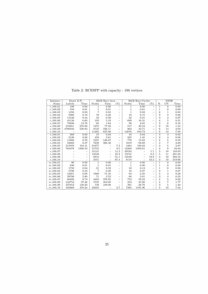
Table 2: RCESPP with capacity - 100 vertices


c 100 01 106 0.00 1 0.00 - 1 0.00 - 1 0 0.00c 100 02 559 0.01 1 0.01 - 1 0.01 - 1 0 0.00c 100 03 1456 0.03 7 0.04 - 1 0.02 - 2 1 0.03c 100 04 5900 0.19 19 0.26 - 10 0.15 - 3 2 0.06c 100 05 11546 0.44 43 0.36 - 22 0.31 - 3 4 0.07c 100 06 45138 6.60 193 5.19 - 699 16.31 - 4 5 0.21c 100 07 75698 13.78 65 1.84 - 99 2.65 - 3 6 0.18c 100 08 310651 276.88 1275 77.50 - 517 30.53 - 6 10 1.34c 100 09 4799333 520.82 8125 326.11 - 862 32.71 - 6 14 2.02c 100 10 - - 11465 627.08 - 12076 910.73 - 6 13 7.68r 100 01 266 0.00 15 0.04 - 10 0.04 - 3 3 0.02r 100 02 2120 0.06 459 3.61 - 225 1.45 - 2 4 0.06r 100 03 11866 0.70 5337 126.87 - 776 15.03 - 4 5 0.59r 100 04 53668 8.37 7639 306.49 - 1819 69.68 - 4 7 2.80r 100 05 215976 104.41 81677 - 7.3 4464 198.93 - 3 5 2.87r 100 06 764476 1300.33 51755 - 9.5 13209 1282.61 - 4 8 34.64r 100 07 - - 31121 - 11.2 29182 - 1.1 5 10 143.63r 100 08 - - 12548 - 25.4 18741 - 6.3 5 11 281.62r 100 09 - - 6912 - 51.1 12549 - 18.9 3 10 303.34r 100 10 - - 2551 - 67.4 6118 - 43.2 3 10 319.68

rc 100 01 90 0.00 1 0.00 - 1 0.00 - 1 0 0.00rc 100 02 636 0.01 1 0.01 - 1 0.00 - 1 0 0.00rc 100 03 1732 0.04 31 0.33 - 10 0.13 - 1 0 0.00rc 100 04 5706 0.23 7 0.20 - 10 0.27 - 2 1 0.07rc 100 05 12561 0.69 1669 71.45 - 64 2.35 - 4 4 0.29rc 100 06 29786 2.80 71 2.52 - 60 3.01 - 3 4 0.35rc 100 07 60499 9.74 4403 376.85 - 752 59.22 - 4 5 0.92rc 100 08 124752 37.46 5735 353.00 - 254 25.00 - 4 7 1.77rc 100 09 237652 130.20 739 109.08 - 391 28.76 - 3 5 1.40rc 100 10 459269 470.24 25055 - 3.7 7385 1191.96 - 5 10 7.33

25

Table 3: RCESPP with distribution and collection - 50 vertices


c 50 01 26 0.00 1 0.00 - 1 0.00 - 1 0 0.00c 50 02 159 0.00 1 0.00 - 1 0.00 - 1 0 0.00c 50 03 554 0.01 1 0.02 - 1 0.01 - 2 1 0.00c 50 04 1751 0.02 7 0.02 - 10 0.04 - 2 1 0.01c 50 05 4675 0.07 15 0.07 - 22 0.10 - 2 2 0.02c 50 06 11311 0.41 27 0.17 - 122 0.94 - 3 3 0.05c 50 07 24006 1.72 17 0.16 - 53 0.48 - 2 3 0.03c 50 08 51401 7.95 83 0.90 - 91 1.44 - 5 7 0.47c 50 09 110354 35.46 69 0.88 - 207 2.47 - 3 5 0.19c 50 10 233478 165.21 119 3.56 - 129 3.66 - 5 10 2.20r 50 01 59 0.00 1 0.00 - 1 0.00 - 1 0 0.00r 50 02 188 0.00 5 0.02 - 7 0.02 - 2 1 0.01r 50 03 486 0.01 1 0.01 - 1 0.01 - 3 3 0.01r 50 04 1113 0.02 1 0.03 - 1 0.03 - 2 3 0.02r 50 05 2085 0.04 11 0.14 - 7 0.08 - 5 6 0.13r 50 06 3882 0.10 17 0.28 - 45 0.62 - 3 5 0.07r 50 07 6986 0.23 3 0.07 - 3 0.08 - 2 4 0.06r 50 08 12138 0.51 71 0.97 - 122 1.13 - 4 7 0.19r 50 09 20384 1.23 13 0.42 - 19 0.59 - 3 7 0.21r 50 10 33107 3.15 5 0.21 - 5 0.21 - 3 7 0.25

rc 50 01 24 0.00 1 0.00 - 1 0.00 - 1 0 0.00rc 50 02 83 0.00 1 0.00 - 1 0.00 - 1 0 0.01rc 50 03 199 0.01 1 0.01 - 1 0.01 - 3 2 0.01rc 50 04 397 0.01 55 0.12 - 73 0.14 - 5 4 0.02rc 50 05 764 0.02 171 0.51 - 114 0.28 - 4 5 0.03rc 50 06 1108 0.02 3321 19.86 - 1156 5.01 - 6 7 0.09rc 50 07 1817 0.03 397 3.00 - 233 1.40 - 6 7 0.09rc 50 08 2546 0.05 595 6.41 - 405 4.07 - 4 7 0.05rc 50 09 3435 0.10 4363 63.94 - 666 8.13 - 7 9 0.22rc 50 10 4998 0.15 12045 210.69 - 6551 79.95 - 6 11 0.24

26

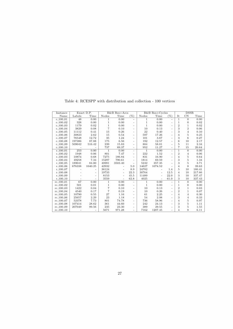
Table 4: RCESPP with distribution and collection - 100 vertices


c 100 01 48 0.00 1 0.00 - 1 0.00 - 1 0 0.00c 100 02 328 0.00 1 0.00 - 1 0.00 - 1 0 0.02c 100 03 1179 0.02 1 0.00 - 1 0.00 - 2 1 0.02c 100 04 3829 0.08 7 0.10 - 10 0.13 - 3 2 0.06c 100 05 11112 0.41 15 0.26 - 22 0.40 - 3 4 0.10c 100 06 30823 2.62 15 0.54 - 597 17.26 - 4 5 0.25c 100 07 76548 12.72 35 1.24 - 101 3.67 - 3 6 0.27c 100 08 197386 87.88 175 6.56 - 192 12.57 - 6 10 2.17c 100 09 509042 516.42 239 15.83 - 884 58.01 - 5 11 2.34c 100 10 - - 737 89.37 - 952 11.27 - 7 15 20.64r 100 01 253 0.00 1 0.00 - 1 0.00 - 1 0 0.00r 100 02 1948 0.06 801 7.47 - 222 1.52 - 2 4 0.06r 100 03 10874 0.68 7275 186.84 - 831 16.90 - 4 5 0.64r 100 04 49258 7.34 15297 790.61 - 1814 69.59 - 3 5 1.34r 100 05 189041 84.00 40991 3503.40 - 5242 357.35 - 3 5 3.71r 100 06 676338 1040.25 42932 - 5.0 14627 1074.52 - 4 8 39.63r 100 07 - - 36124 - 8.9 24782 - 1.4 5 10 180.41r 100 08 - - 19733 - 22.3 30764 - 12.5 4 10 217.66r 100 09 - - 8153 - 45.5 11489 - 22.0 3 10 337.47r 100 10 - - 3559 - 62.8 4025 - 61.0 3 10 337.43

rc 100 01 67 0.00 1 0.00 - 1 0.00 - 1 0 0.00rc 100 02 501 0.01 1 0.00 - 1 0.00 - 1 0 0.00rc 100 03 1422 0.04 7 0.10 - 10 0.13 - 2 1 0.03rc 100 04 4540 0.17 7 0.19 - 10 0.26 - 2 1 0.07rc 100 05 10790 0.55 27 1.16 - 61 2.25 - 4 4 0.30rc 100 06 25657 2.29 23 1.18 - 54 2.98 - 3 4 0.33rc 100 07 52378 7.73 801 74.78 - 736 58.96 - 4 5 0.97rc 100 08 107414 28.62 361 44.60 - 242 24.13 - 3 5 1.11rc 100 09 207049 99.56 235 23.30 - 389 29.55 - 3 5 1.55rc 100 10 - - 5671 971.28 - 7162 1207.45 - 4 8 6.11

27

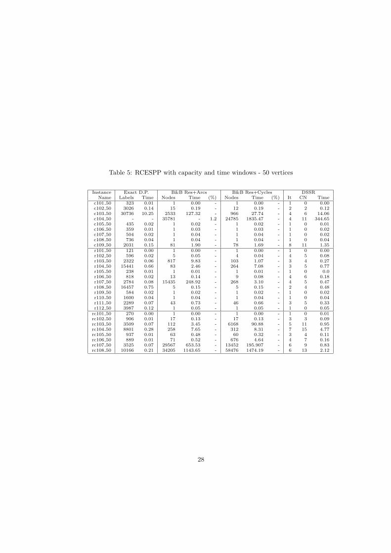
Table 5: RCESPP with capacity and time windows - 50 vertices


c101 50 323 0.01 1 0.00 - 1 0.00 - 1 0 0.00c102 50 3026 0.14 15 0.19 - 12 0.19 - 2 2 0.12c103 50 30736 10.25 2533 127.32 - 966 27.74 - 4 6 14.06c104 50 - - 35781 - 1.2 24785 1835.47 - 4 11 344.65c105 50 435 0.02 1 0.02 - 1 0.02 - 1 0 0.01c106 50 359 0.01 1 0.03 - 1 0.03 - 1 0 0.02c107 50 504 0.02 1 0.04 - 1 0.04 - 1 0 0.02c108 50 736 0.04 1 0.04 - 1 0.04 - 1 0 0.04c109 50 2031 0.15 81 1.90 - 78 1.69 - 8 11 1.35r101 50 121 0.00 1 0.00 - 1 0.00 - 1 0 0.00r102 50 596 0.02 5 0.05 - 4 0.04 - 4 5 0.08r103 50 2322 0.06 817 9.83 - 103 1.07 - 3 4 0.27r104 50 15441 0.66 83 2.46 - 264 7.08 - 3 5 0.77r105 50 238 0.01 1 0.01 - 1 0.01 - 1 0 0.0r106 50 818 0.02 13 0.14 - 9 0.08 - 4 6 0.18r107 50 2784 0.08 15435 248.92 - 268 3.10 - 4 5 0.47r108 50 16457 0.75 5 0.15 - 5 0.15 - 2 4 0.48r109 50 584 0.02 1 0.02 - 1 0.02 - 1 0 0.02r110 50 1600 0.04 1 0.04 - 1 0.04 - 1 0 0.04r111 50 2289 0.07 43 0.73 - 46 0.66 - 3 5 0.33r112 50 3987 0.12 1 0.05 - 1 0.05 - 1 0 0.05

rc101 50 270 0.00 1 0.00 - 1 0.00 - 1 0 0.01rc102 50 906 0.01 17 0.13 - 17 0.13 - 3 3 0.09rc103 50 3509 0.07 112 3.45 - 6168 90.88 - 5 11 0.95rc104 50 8801 0.28 258 7.65 - 312 8.31 - 7 15 4.77rc105 50 937 0.01 63 0.48 - 60 0.32 - 3 4 0.11rc106 50 889 0.01 71 0.52 - 676 4.64 - 4 7 0.16rc107 50 3525 0.07 29567 653.53 - 13452 195.907 - 6 9 0.83rc108 50 10166 0.21 34205 1143.65 - 58476 1474.19 - 6 13 2.12

28

Table 6: RCESPP with capacity and time windows - 100 vertices


c101 100 679 0.06 1 0.02 - 1 0.02 - 1 0 0.02c102 100 11839 2.99 15 0.89 - 12 0.67 - 2 2 0.63c103 100 123804 133.56 2539 507.78 - 3075 485.68 - 5 9 40.15c104 100 - - 17553 - 17.8 23402 - 16.5 4 11 311.44c105 100 915 0.11 1 0.06 - 1 0.06 - 1 0 0.06c106 100 1159 0.16 1 0.07 - 1 0.07 - 1 0 0.07c107 100 1058 0.16 1 0.08 - 1 0.08 - 1 0 0.08c108 100 1690 0.33 1 0.17 - 1 0.17 - 1 0 0.17c109 100 4608 1.28 111 14.18 - 101 12.66 - 8 13 9.19r101 100 452 0.01 1 0.00 - 1 0.00 - 1 0 0.00r102 100 14792 2.21 4203 438.82 - 1003 96.25 - 3 6 21.69r103 100 135575 95.73 377 128.71 - 252 61.10 - 4 7 159.74r104 100 655858 1242.56 4531 - 0.9 1945 1013.04 - 3 5 78.32r105 100 1161 0.06 1 0.03 - 1 0.03 - 1 0 0.03r106 100 22970 5.52 26059 - 3.4 3344 467.29 - 4 7 71.60r107 100 138027 100.83 1417 717.37 - 732 232.91 - 4 12 335.98r108 100 570910 891.81 1593 1098.05 - 1451 611.61 - 3 5 146.58r109 100 3504 0.37 49 3.39 - 49 3.45 - 3 5 2.93r110 100 25063 4.89 307 69.25 - 406 77.55 - 3 6 19.31r111 100 69890 25.86 2669 866.34 - 361 129.24 - 3 7 53.16r112 100 394702 647.36 2167 2227.74 - 665 385.00 - 3 9 340.61

rc101 100 955 0.03 1 0.02 - 1 0.02 - 1 0 0.02rc102 100 5384 0.30 17 1.12 - 21 1.34 - 4 4 3.17rc103 100 38308 6.01 861 110.78 - 6494 587.39 - 4 8 35.37rc104 100 232961 148.73 607 194.68 - 1054 203.36 - 4 8 102.56rc105 100 2964 0.15 7 0.43 - 13 0.67 - 4 6 1.14rc106 100 2574 0.12 31 1.85 - 12 0.56 - 3 3 1.01rc107 100 10505 0.72 87 8.50 - 27 2.79 - 4 6 3.65rc108 100 45430 6.75 239 32.34 - 143 12.43 - 3 5 4.84

29

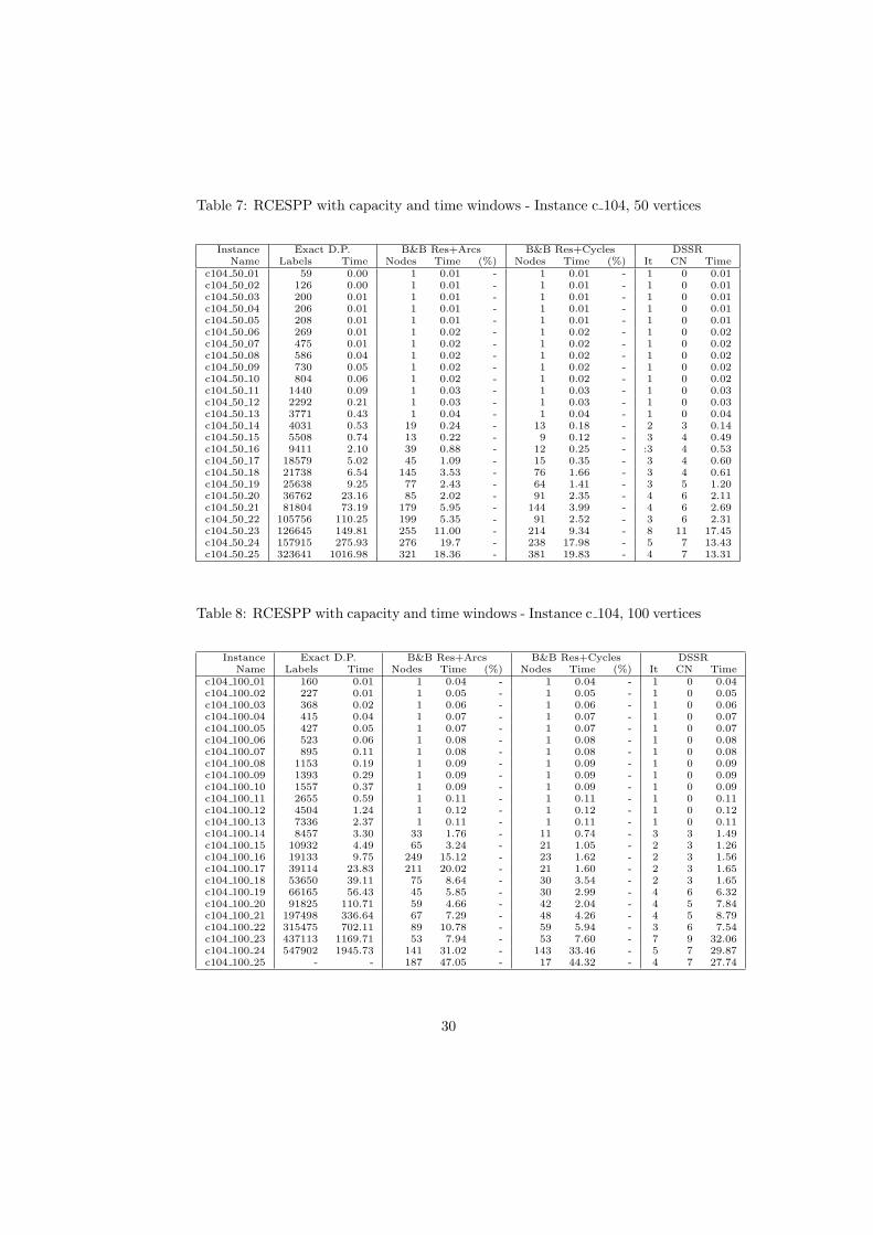
Table 7: RCESPP with capacity and time windows - Instance c 104, 50 vertices


c104 50 01 59 0.00 1 0.01 - 1 0.01 - 1 0 0.01c104 50 02 126 0.00 1 0.01 - 1 0.01 - 1 0 0.01c104 50 03 200 0.01 1 0.01 - 1 0.01 - 1 0 0.01c104 50 04 206 0.01 1 0.01 - 1 0.01 - 1 0 0.01c104 50 05 208 0.01 1 0.01 - 1 0.01 - 1 0 0.01c104 50 06 269 0.01 1 0.02 - 1 0.02 - 1 0 0.02c104 50 07 475 0.01 1 0.02 - 1 0.02 - 1 0 0.02c104 50 08 586 0.04 1 0.02 - 1 0.02 - 1 0 0.02c104 50 09 730 0.05 1 0.02 - 1 0.02 - 1 0 0.02c104 50 10 804 0.06 1 0.02 - 1 0.02 - 1 0 0.02c104 50 11 1440 0.09 1 0.03 - 1 0.03 - 1 0 0.03c104 50 12 2292 0.21 1 0.03 - 1 0.03 - 1 0 0.03c104 50 13 3771 0.43 1 0.04 - 1 0.04 - 1 0 0.04c104 50 14 4031 0.53 19 0.24 - 13 0.18 - 2 3 0.14c104 50 15 5508 0.74 13 0.22 - 9 0.12 - 3 4 0.49c104 50 16 9411 2.10 39 0.88 - 12 0.25 - :3 4 0.53c104 50 17 18579 5.02 45 1.09 - 15 0.35 - 3 4 0.60c104 50 18 21738 6.54 145 3.53 - 76 1.66 - 3 4 0.61c104 50 19 25638 9.25 77 2.43 - 64 1.41 - 3 5 1.20c104 50 20 36762 23.16 85 2.02 - 91 2.35 - 4 6 2.11c104 50 21 81804 73.19 179 5.95 - 144 3.99 - 4 6 2.69c104 50 22 105756 110.25 199 5.35 - 91 2.52 - 3 6 2.31c104 50 23 126645 149.81 255 11.00 - 214 9.34 - 8 11 17.45c104 50 24 157915 275.93 276 19.7 - 238 17.98 - 5 7 13.43c104 50 25 323641 1016.98 321 18.36 - 381 19.83 - 4 7 13.31

Table 8: RCESPP with capacity and time windows - Instance c 104, 100 vertices


c104 100 01 160 0.01 1 0.04 - 1 0.04 - 1 0 0.04c104 100 02 227 0.01 1 0.05 - 1 0.05 - 1 0 0.05c104 100 03 368 0.02 1 0.06 - 1 0.06 - 1 0 0.06c104 100 04 415 0.04 1 0.07 - 1 0.07 - 1 0 0.07c104 100 05 427 0.05 1 0.07 - 1 0.07 - 1 0 0.07c104 100 06 523 0.06 1 0.08 - 1 0.08 - 1 0 0.08c104 100 07 895 0.11 1 0.08 - 1 0.08 - 1 0 0.08c104 100 08 1153 0.19 1 0.09 - 1 0.09 - 1 0 0.09c104 100 09 1393 0.29 1 0.09 - 1 0.09 - 1 0 0.09c104 100 10 1557 0.37 1 0.09 - 1 0.09 - 1 0 0.09c104 100 11 2655 0.59 1 0.11 - 1 0.11 - 1 0 0.11c104 100 12 4504 1.24 1 0.12 - 1 0.12 - 1 0 0.12c104 100 13 7336 2.37 1 0.11 - 1 0.11 - 1 0 0.11c104 100 14 8457 3.30 33 1.76 - 11 0.74 - 3 3 1.49c104 100 15 10932 4.49 65 3.24 - 21 1.05 - 2 3 1.26c104 100 16 19133 9.75 249 15.12 - 23 1.62 - 2 3 1.56c104 100 17 39114 23.83 211 20.02 - 21 1.60 - 2 3 1.65c104 100 18 53650 39.11 75 8.64 - 30 3.54 - 2 3 1.65c104 100 19 66165 56.43 45 5.85 - 30 2.99 - 4 6 6.32c104 100 20 91825 110.71 59 4.66 - 42 2.04 - 4 5 7.84c104 100 21 197498 336.64 67 7.29 - 48 4.26 - 4 5 8.79c104 100 22 315475 702.11 89 10.78 - 59 5.94 - 3 6 7.54c104 100 23 437113 1169.71 53 7.94 - 53 7.60 - 7 9 32.06c104 100 24 547902 1945.73 141 31.02 - 143 33.46 - 5 7 29.87c104 100 25 - - 187 47.05 - 17 44.32 - 4 7 27.74

30

Documents

New dynamic programming algorithms for the resource