Embed Size (px)
Citation preview
REVIEW ARTICLE
New estimates of potential impacts of sea level riseand coastal floods in Poland
Dominik Paprotny1• Paweł Terefenko2
Received: 19 November 2015 / Accepted: 6 October 2016 / Published online: 15 October 2016� The Author(s) 2016. This article is published with open access at Springerlink.com
Abstract Polish coastal zone is thought to be one of the most exposed to sea level rise in
Europe. With mean sea levels expected to increase between 28 and 98 cm by the end of the
century, and storms increasing in severity, accurate estimates of the consequences of those
phenomena are needed. Recent advances in quality and availability of spatial data in
Poland made possible the reassessment of previous estimates of inundation caused by sea
level rise. Up-to-date, detailed information on land use, population and buildings was used
here to calculate their exposure to floods at a broad range of scenarios. Inclusion of a high-
resolution digital elevation model contributed to a further improvement in estimates. The
results revealed that even by using a static ‘‘bathtub fill’’ approach, the amount of exposed
land, population or assets is significantly smaller than indicated in previous assessments. In
the perspective of the twenty-first century, direct damages caused by sea level rise will be
small and adaptation costs will not be significant. However, the increase in the frequency
of storm surges could elevate the risk to the population and economy, but cost-effective
flood protection measures would be able to mitigate the risk. The exposure of different
kinds of assets and sectors of the economy varies to a large extent, though the structural
breakdown of potential losses is remarkably stable between scenarios.
Keywords Sea level rise � Coastal floods � Poland � Flood risk � GIS
Electronic supplementary material The online version of this article (doi:10.1007/s11069-016-2619-z)contains supplementary material, which is available to authorized users.
& Dominik [email protected]
1 Department of Hydraulic Engineering, Faculty of Civil Engineering and Geosciences,Delft University of Technology, Stevinweg 1, 2628 CN Delft, The Netherlands
2 Remote Sensing and Marine Cartography Unit, Faculty of Geosciences, University of Szczecin,Mickiewicza 18, 70-383 Szczecin, Poland
123
Nat Hazards (2017) 85:1249–1277DOI 10.1007/s11069-016-2619-z

1 Introduction
Storms surges are an important factor shaping the Polish coast. Short-term water level
variations caused by them significantly alter the coast in the non-tidal Baltic Sea, where
extreme water levels depend largely on the volume of water flowing in from the North Sea.
Several large coastal floods occurred in late nineteenth and early twentieth century, with a
few calmer decades thereafter. More recently, however, storms have been on the rise: the
number of surges exceeding the warning level of approximately 70 cm above mean sea
level (MSL) soared from about two per year in the 1950s to six per year in 2000s (Wis-
niewski and Wolski 2009). Usually these events are too short to cause damages inland.
However, during a storm surge in January 1983 water levels exceeded 1.3 m above MSL
along the most of the coast, affecting many locations, particularly in the eastern part. In the_Zuławy region, a total of 50 km2 of land was flooded and almost 1300 people were
evacuated (Bednarczyk et al. 2006). Wisniewski and Wolski (2009) estimated that a
100-year coastal flood could be as high as 1.95 m above average in Kołobrzeg, while a
1000-year flood might reach 2.5 m; the highest value actually recorded was 2.22 m in
1872.
Long-lasting storm surges, even though relatively insignificant at the coast, can cause a
flood dozens of kilometres inland, on the low-lying parts of Odra and Vistula fluvial plains.
In those estuaries, water levels could even be higher than at the coast; this happens when
large volumes of water flow in from the sea due to the northerly winds (Wisniewski and
Kowalewska-Kalkowska 2007). The highest recorded water level in Szczecin, located
almost 70 km inland, was 1.54 m above average during a storm surge in 1913 (Richter
et al. 2012). The most recent storm surge resulting in a large inflow of seawater into the
river network occurred in 2009, causing losses of several million euro in locations all over
the coast, mainly in the eastern part (KZGW 2011). Across the whole region, flood
defences protect the lowest areas, particularly around river mouths and coastal lakes, while
the rest of the coast is protected by nature.
At a longer timescale, the contemporary sea level rise (SLR) triggered by the changing
climate is also a threat to coastal areas. It is generally considered (Church et al. 2013;
Hunter 2010; Wroblewski 1994) that the increase in mean sea level will directly translate
into higher storm surge maxima. It is therefore necessary to assess the number of persons
and value of assets which could be at stake. In Poland, comprehensive research on coastal
flood risk considering sea level rise was originally spawned by IPCC’s first assessment
report released in 1990. Rotnicki and Borowka (1991) used 1:25,000 topographic maps to
calculate the area threatened by rising waters along with a quantification of assets affected,
such as land use, infrastructure, settlements and their population. According to an
expanded version of that study (Rotnicki et al. 1995), a 2.5-m SLR would impact 2700 km2
of land, including 93 km2 of settlements, 374 km of railways, 906 km of roads and
297,000 people. Based on the results of Rotnicki’s and Borowka’s (1991) study, Pluijm
et al. (1992) calculated the monetary value of land and structures exposed to sea level rise.
The results indicated that a 1-m rise of mean sea levels would result in a loss of assets
worth 24 % of 1990 gross domestic product (GDP). This study was later updated with
newer economic data by Zeidler (1997), whose results were in turn reused by Pruszak and
Zawadzka (2005, 2008) and cited in several global assessments of sea level rise (e.g.
Nicholls and Mimura 1998; Nicholls and Klein 2005). In effect, published assessments of
the effects of sea level rise are limited to delimitations of hazard zones made in late 1980s
(the earliest version of the study by Rotnicki and Borowka was published in 1989) and
1250 Nat Hazards (2017) 85:1249–1277
123

socio-economic data from the early 1990s. Poland was included in studies on global and
European flood risk based on DIVA model—most recently by Hinkel et al. (2014)—though
only Hinkel et al. (2010) and Bosello et al. (2012) included a breakdown of impacts by
country. All of these studies used only low-resolution data and were characterized by a
high degree of generalization. For instance, only a most recent analysis (Mokrech et al.
2015) included flood defences in the calculation of flood hazard in Europe and only using
assumptions of protection levels. Still, no information on country-level impacts was
provided.
More recently, due to the obligations imposed by the European Union’s ‘‘flood direc-
tive’’ (EU 2007), the national government ordered preparation of flood risk maps for
selected regions of Poland. They were published in 2013 by the National Water Man-
agement Authority (KZGW 2015). Their main advantage is the use of up-to-date, detailed
and high-resolution data, including lidar-derived digital elevation models (DEMs), aerial
photography, land surveys and administrative registers. However, the main focus has been
put on river floods, while only parts of the coast were investigated. Moreover, no sea level
rise impacts were assessed, while the analysis of storm surges was limited only to one or
two scenarios, depending on location. Finally, the results of flood risk calculations are
provided only as a graphical representation on maps, and the only aggregate statistics
provided are the estimates of exposed inhabitants per settlement. The total value of
exposed assets was not disclosed.
In the light of the above, there is clearly a need for a high-resolution assessment of
possible social and economic impacts of storm surges and inundation of land caused by sea
level rise in Poland. This is particularly important as the existing studies all indicated that
very severe consequences for the population and economy might occur in the twenty-first
century. In this paper, we aim to provide more precise estimates of exposure of land,
population and assets at a broad range of scenarios, using the up-to-date and detailed
cartographic materials, which have become available only recently. Most importantly, the
digital elevation model used here includes the majority of flood defences in the area, which
were missing in other studies. The main aim is to provide a dataset, which could be used to
various, frequently changing, projections of climate, population and economic growth.
Furthermore, we analyse the data in the context of IPCC projections, as well as discuss the
adaptation measures.
2 Materials and methods
2.1 Regional setting
The Baltic Sea is a non-tidal, semi-enclosed and shallow body of brackish water. Exchange
of water through the Danish Straits is the primary regulator of water levels in the basin,
causing dangerous surges primarily at its southern and eastern coasts (Ekman 2009; Wolski
et al. 2014). Poland has a 500-km-long, diversified coastline. At various locations along the
coast, there are sections of cliffs totalling ca. 18 % of entire coastline length (Tomczak
1995). Apart from an alluvial section in the Puck Lagoon (less than 3 % of the total), the
remainder is a spit- and barrier-type coast, with dunes ranging in height from less than 2 up
to 49 m. Behind the dunes, coastal plains with occasional depressions (down to -1.8 m
MSL) are usually observed.
Nat Hazards (2017) 85:1249–1277 1251
123

Tide gauge in Swinoujscie, at mouth of Odra Estuary in the Baltic Coast, has one of the
longest instrumental records in the world (Permanent Service for Mean Sea Level 2015),
and during 1811–2006, a trend of 0.4 mm per year was observed here, accelerating to
1.0 mm per year during 1947–2006 (Wisniewski et al. 2011). This rate rises moving
eastward: Kołobrzeg (central part of the Polish coast) recorded an increase of 0.5 mm
during 1901–2006 and 1.4 mm during 1947–2006, while in Gdansk (eastern coast),
1.6 mm increase was observed during 1886–2006 and 2.5 mm during 1947–2006. The
difference is largely due to uneven isostatic movement of the crust. Global mean sea level
has risen by 21 cm between 1880 and 2009 (Church and White 2011), or 1.6 mm per year.
Also, satellite altimetry reveals that the rise in water levels is mostly uniform in the
southern Baltic Sea. It amounted to 3.2 mm per year between 1992 and 2016, a pace very
similar to the world ocean average, which was 2.9 mm per year during 1992–2016 (NOAA
2016).
Although as much as 7 % of world population lives within 20 km from the coast
(Kummu et al. 2016), the Polish Baltic Sea coast itself is not densely inhabited: only 2.8 %
of Poles reside in municipalities with direct access to the sea. Excluding the large Tricity
agglomeration (Gdansk, Sopot, Gdynia), the population density in this area is a mere 90
persons per km2 which is quite low when compared to the national average of 123 (CSO
2015). However, the coast is by far the most popular vacation destination in Poland. Thirty-
five percentage of all overnight stays in accommodation establishments during July–Au-
gust 2013 occurred in 55 municipalities considered by Eurostat as coastal regions (CSO
2015). That corresponds to an average of 71 tourists per 100 residents during the summer.
The economies of many coastal resorts are completely dependent on this short holiday
season (Łonyszyn and Terefenko 2014). Any damages to infrastructure and buildings could
therefore dampen the economic prospects of those localities.
The study area, as referred to hereafter, includes all municipalities, not necessarily
bordering the Baltic Sea, in which there is some land laying no more than 5 m above mean
sea level. There are 86 such municipalities, including 22 that further divide into a town and
a rural area. That sums up to 108 basic administrative units with a combined population of
2.4 million (at 2011 census according to CSO 2015). Figure 1 outlines the study area
within the Polish coastal zone.
2.2 Data sources
Two main sources of data were used in this study: the topographic objects database
containing information on land use as well as buildings, and a digital elevation model
(DEM). Both were derived from national cartographic repository (CODGiK 2014, 2016),
which include recent output of large-scale mapping projects. Statistical data on demo-
graphic and economic indicators have also been collected.
2.2.1 Digital elevation models
Quality of flood hazard analyses depends mainly on detailed information on the terrain in
question. Here, a digital elevation model created through airborne laser scanning tech-
nology (lidar) was used. DEMs obtained using this method are commonly applied to
coastal flood hazard analyses because of their accuracy (Webster 2010). In recent years, the
national government launched a large measurement campaign specifically to provide data
for flood hazard mapping, which was carried out in the coastal areas between 2010 and
2013 (mainly in 2011). The density of scanning was usually 4 points per m2, except for
1252 Nat Hazards (2017) 85:1249–1277
123

urban agglomerations, where the density was 12 points per m2. The final dataset in raster
format has a spatial resolution of 1 m, which is fine enough to include flood defences and
most of other small topographic features that can have a profound impact on flood hazard
analyses. Average vertical error of the dataset is nominally less than 20 cm in areas with
scanning density of 4 pts/m2 and less than 10 cm in areas scanned with 12 pts/m2
(CODGiK 2014). Yet, the DEM has some other imperfections. A large low-lying area,
which in reality is protected by higher terrain or flood defence structures, can be marked as
potentially flooded if a minor error in the data creates a ‘‘gate’’ for floodwater. Also, some
of the hydraulic structures used to manage river flow and maritime transport, such as locks,
sluices and weirs, are mostly not present in the DEM.
A very small area located in the western part of the coastal zone is not covered by the
detailed lidar DEM. The gap was filled with a different DEM, which was created on the
basis of aerial photographs. It has a spatial resolution of 40 m and a vertical accuracy of
about 1.5 m. These are much worse values than for the lidar DEM, but it had to be used
only for less than 0.1 % of the exposed area, so it has a negligible impact on the results.
2.2.2 Topographic objects database
The primary source of information on land use and buildings used here is the topographic
objects database, the digital successor of analogue topographic maps, created and main-
tained by Poland’s surveyor general (CODGiK 2016). It consists of almost 300 types of
objects with a vectorized representation of their geometry and additional qualitative and
quantitative descriptors. Accuracy of the database in terms of location and minimum size
of objects approaches a 1:10,000 topographic map. This is enough to represent the natural
and socio-economic environment down to a single parcel, road and building. The current
structure of the database was implemented in 2011 (Law 2011/279/1642), and its content
was updated during 2012–2013. The database used here corresponds to the state of
Fig. 1 Study area (all municipalities with some land lying below ?5 m MSL) and the Polish coastal zone.The inner map presents elevation values
Nat Hazards (2017) 85:1249–1277 1253
123

January–July 2013, depending on location. Quantitative information on the objects, such as
their area, is expected not to deviate from real values more than ±20 %.
Data on buildings include their area, functional characteristic and, in most cases, the
number of storeys. In case the latter is missing, the building was assumed to have only one
storey. Roads are represented in the database as a linear object, but for each section, their
width is given, so that they could be transformed into a surface. Only paved roads were
included in the calculation. Railway and tramlines were transformed into polygons
according to the gauge of the tracks. Roads and tracks located on bridges or similar above-
ground structures were excluded.
2.3 Calculation of flood hazard
2.3.1 Inundation
Flood hazard analysis involves calculation of the inundation extent and other hydrological
parameters of the flooding, such as water depth. To calculate the flood zone, a ‘‘bathtub
fill’’ approach was applied for this study (Bates and De Roo 2000; Poulter and Halpin
2008). It is assumed that the sea at a certain scenario will cover all land lying below the
assumed water level, as long as there is a direct connection with the source of flood. For the
analysis of inundation caused by sea level rise, that is an accurate description. However,
for storm surges it is a straightforward simplification. The method does not take into
account the kinematics of the flow or sedimentation processes and considers flooding as an
instantaneous process. The temporal change in water levels is also an important factor
determining the inundation extent. Unfortunately, the data required to include time in such
a calculation were not available to the authors. In effect, the storm surge scenarios con-
stitute a description of the worst-case event (Apel et al. 2009; Breilh et al. 2013). The
biggest advantage of the chosen method is a possibility of a direct comparison of achieved
results with previous studies performed in the Baltic coast. The possibility of directly
implementing the method in the geographical information systems is also useful. On the
other hand, dynamic effects such as erosion and sedimentation were not included.
The resolution of the DEM is fine enough to include flood defences; therefore, isolated
locations, i.e. having no direct connection with the sea, lying below the water level at a
given scenario were considered protected by the surrounding high terrain. These areas were
discarded to create the final flood zone using a four-side rule, which means that no water
flow was allowed in diagonal directions (Poulter and Halpin 2008). Naturally, dikes and
other structures could fail and flood the hinterland, but that aspect was not considered in
this article. Also, the situation when water floods the land behind structures through
culverts was not analysed. Protection from flood defences such as dikes, banks and other
earthworks, as well as sluices and weirs is included in the calculation.
The GIS analysis itself was performed using the ArGIS 10 software. Raster datasets
with information on elevation (CODGiK 2014) were combined to generate a complete grid
of the study area. The grid was then reclassified into two distinct classes: above and below
the analysed sea level. The result was a two-coloured map showing the land and the
inundation. The latter class was transformed into a vector polygon, and its connection with
the sea was investigated by selecting only those polygons that are intersecting with the
water at normal level. The resulting polygons were clipped with a mask representing Polish
borders in order to delimit the final area at country level. Further analysis included
intersections between inundated area for each water level and different layers representing
buildings, land types, etc. extracted from the topographic objects database (CODGiK 2016)
1254 Nat Hazards (2017) 85:1249–1277
123

as well as grouping the results into different systematic classes according to administrative
divisions.
2.3.2 SLR and storm surge scenarios
Sea level rise and storm surges were analysed in intervals of 5 cm, providing scenarios of
5, 10, 15, etc., cm up to 5 m above mean sea level. In this way, the exposure of population
and assets at different elevations could be assessed in detail. The 5-m value was chosen as
the rounded value of the maximum possible SLR indicated in the literature (1.4–2 m in
Rahmstorf 2007; Pfeffer et al. 2008) together with a 1000-year coastal flood (about ?2.5 m
MSL according to Wolski et al. 2014). Mean sea level along the Polish coast varies
slightly, with 1947–2006 average in Gdansk being 7 cm higher than in Swinoujscie
(Wisniewski and Wolski 2009). As a minor simplification, the 500 cm ‘‘baseline’’ level of
all Polish tide gauges was used here as MSL, which corresponds to about ?0.10 m in the
European Vertical Reference System EVRS-2007 (Urbanski 2012).
The results are also juxtaposed here with future sea level rise scenarios included in the
latest IPCC report (Church et al. 2013). Three scenarios are considered: the medium
projection for RCP4.5 and the lowest and highest of the projections (lower bound of
RCP2.6 and upper bound of RCP8.5). In those scenarios, water levels rise gradually to 28,
53 and 98 cm SLR by 2100 relative to 1986–2005 levels. However, Polish coast is subject
to the glacial isostatic adjustment, which causes a yearly uplift by about 0.4–0.5 mm
(Peltier et al. 2015). Increase in water levels is also uneven regardless of the movement of
the coast; satellite-measured SLR trend during 1992–2015 was between 4.2 and 4.3 mm
per year in the Baltic along the Polish coast; only in the far western part, it was slightly
higher, up to 4.5 mm per year (NOAA 2016). These two effects translate to a difference of
only a few centimetres in a perspective of a century. Bigger spatial differences in SLR can
be caused by ground subsidence, which is a very local factor; no large-scale data are
available on this matter. Therefore, IPCC scenarios were applied in the analysis without
modifications.
For the analysis of coastal floods, the return periods of storm surges were calculated.
They vary along the coast and lagoons; therefore, the return periods were calculated from
annual maximum water levels recorded at eight gauges during 1948–2007. To each station
(5 coastal, 1 in the Szczecin Lagoon and two on Odra river), the nearest basic adminis-
trative units were assigned. Water level data from Wisniewski and Wolski (2009) were
used and fitted to Gumbel probability distribution; details on the methodology can be found
in Paprotny (2014).
2.4 Calculation of flood risk
Flood risk is a combination of three elements, as follows:
• Hazard, i.e. factor that can cause adverse effects, in our case sea level rise and coastal
floods (see previous section);
• Exposure, i.e. the inventory of elements that could potentially be affected by the
hazard;
• Vulnerability, i.e. the propensity of exposed elements to be adversely affected by the
hazard event (Kron 2005; Cardona et al. 2012).
Nat Hazards (2017) 85:1249–1277 1255
123

In this section, we present the methodology to calculate exposure and vulnerability in
order to obtain an estimate of risk caused by sea level rise and coastal floods in context of
SLR.
2.4.1 Calculation of exposure
Following Hallegatte’s (2012) framework on investigating impact of SLR on economic
growth, we analyse exposure to the following elements:
• Permanent losses of natural capital: market value of land, including an estimate of the
area of protected habitats,
• Permanent loss of physical capital: gross replacement cost of immovable and movable
fixed assets,
• Permanent loss of social capital: number of inhabitants.
Value of aforementioned assets was calculated here using 2011 data, the latest year for
which complete statistics required here were available. The primary source was the online
databases of the Central Statistical Office of Poland (CSO 2015). Values of land under
different types of use are an estimate of their 2011 market price. Average sale price
calculations made by CSO were used for arable land, meadows and pastures. Value of
forests was taken from estimates of the State Forests, the manager of the vast majority of
Polish woods (Ministry of Treasury 2012). Their calculations include both the value of
land parcels and the trees covering them. Value of areas covered by buildings, transport
infrastructure or non-built-up areas ready for construction was estimated using the relation
between the sale price of those types of land use and the sale price of arable land in
Germany in 2011 (Statistisches Bundesamt 2015). For other types of land use, numbers
were assigned based on governmental regulations on estimation of real estate value (Law
2004/207/2109). As a result, woodlands or bushes are assumed to be worth equal to poor-
quality arable land. Orchards were assigned the same value as arable land, while waste-
lands and other unutilized land were considered as equal to poor-quality meadows. Loss of
inland surface water was not taken into consideration. Summary of land values is presented
in Table 1. Agricultural build-up areas do not form a separate category in the topographic
database; it was assumed that build-up areas adjacent to arable land and permanent crops
fall into this category.
Table 1 Estimated commercialvalue of land in 2011 per hectare,in Zloty (the polish national cur-rency, PLN)
4.12 PLN = €1
Land use Value (PLN per ha)
Built-up: services 4,294,000
Built-up: housing (dense urban) 2,802,000
Built-up: housing (scattered urban) 1,896,000
Transport areas, non-built-up areas 559,000
Built-up: agricultural 453,000
Built-up: industrial 444,000
Forests 37,976
Arable land, orchards 20,004
Woodlands and bushes 16,401
Meadows and pastures 14,259
Wastelands and other lands 12,337
1256 Nat Hazards (2017) 85:1249–1277
123
Information on buildings was compiled from several sources in order to calculate their
value relative to their area (Table 2). Value of housing is the average construction cost of
new houses as calculated by CSO. Stock of movable assets is difficult to estimate, and no
national statistics in this matter are available. However, the ratio between household
durable goods’ value and GDP is reported to differ only slightly between countries and
throughout modern history (Piketty and Zucman 2014). It was therefore assumed that the
total value in this category in Poland constitutes 35 % of GDP, which is the average ratio
in four countries (Canada, Germany, UK and USA) for which data are provided by Piketty
and Zucman (2014). GDP and housing area statistics from CSO were used in order to
obtain the amount of movable assets per m2 in 2011.
Commercial buildings were divided into three branches (industry, services and agri-
culture), and for each type, its value was calculated using the following formula:
V ¼ F � Ls
L� As
ð1Þ
where V is the value of a building per area in PLN, F is the value of fixed assets in Poland,
Ls is the corresponding land use area in the study area, L is the corresponding land use area
in Poland, and As is the total building area in the study area. Fixed assets estimates were
obtained from Eurostat (2015). Land use data for Poland is from CSO (2015), while for the
study area, the corresponding types of land use from the topographic database were used.
Finally, building area was extracted from the topographic database, taking into account the
multiple storeys several buildings contain.
2.4.2 Calculation of vulnerability
Assumptions on vulnerability of land and assets are presented in Table 3. In case of rising
average water levels, land and immovable fixed assets (i.e. buildings and structures) are
covered permanently by water and therefore lost completely. Movable fixed assets, which
include machine tools, household goods, vehicles or livestock, can be evacuated from the
endangered area given the gradual nature of SLR. Therefore, no losses in this category are
Table 2 Value of fixed assets per area in 2011 and damage functions
Type of building or structure Value of fixed assets Damage function
Immovable(PLN per m2)
Movable(PLN per m2)
Y—damage (%),D—water depth (m)
Housing 3858 604 Y1 ¼ Dþ 18:77 �ffiffiffiffi
Dp
Y2 ¼ 4:83 � Dþ 20:69 �ffiffiffiffi
Dp
Industry 2057 1712 Y ¼ 27 �ffiffiffiffi
Dp
Services 2678 923 Market services: Y ¼ 27 �ffiffiffiffi
Dp
Non-market services: Y ¼ 30 �ffiffiffiffi
Dp
Agriculture 393 166 Y ¼ 27 �ffiffiffiffi
Dp
Transport infrastructure 436 – Y ¼ 1003
For housing, Y1 is damage to immovable assets and Y2 is damage to movable assets
Nat Hazards (2017) 85:1249–1277 1257
123

assumed. In case of coastal floods, no losses are assumed for land, as water covers it only
temporarily. Some productivity of land may be lost and consequently its market value
could decrease; however, this aspect was not analysed here. Damage to crops is not
analysed too, as they are not considered fixed assets, similarly to stocks of produced goods.
Losses of fixed assets are calculated using damage functions, which relate losses to water
depths (Apel et al. 2009).
Damage functions, which relate water depth to the relative loss of assets, were applied
from Emschergenossenschaft/Hydrotec (2004), who created them using HOWAS database
of flood losses (Merz et al. 2004). They were selected for this study, because there are no
corresponding functions created from Polish empirical data. Additionally, they are similar
to damage curves created as a combination of various European methodologies by Hui-
zinga (2007) and suggested for use in countries without national damage functions. The
only exception is the damage function for transportation, which is a constant value rather
than a damage function. As can be noticed in Table 2, the equations differ for immovable
and movable housing assets, while for commercial activity, they are combined. Finally, the
value of transport infrastructure was taken from official risk calculations, according to the
Polish government’s methodology (Law 2013/104). Total value of losses for a building can
be described as:
R ¼ A� V � Y Dð Þ ð2Þ
where R is the total loss for a building in PLN, A is the building area (including all
storeys), V is the total value of the building per area, and Y(D) is the appropriate damage
function for water depth D (averaged within the building’s contour).
Additionally, the number of people affected by sea level rise and coastal floods was
estimated. Population data from the 2011 census (CSO 2015) provide information down to
settlement level. By combining these data with housing area from the topographic objects
database, it was possible to further disaggregate the data and obtain the average number of
persons per housing area in settlements and towns. All persons living in a residential
building even partially covered by water were assumed as being affected by the event.
Similarly, the amount of tourism traffic potentially lost was estimated by disaggregating
the number of tourists and nights spent in establishments (at basic administrative unit-
level) using the size of appropriate categories of buildings. For the purpose of this study,
‘‘tourists’’ refer only to persons staying overnight in collective accommodation, excluding
persons in camping sites.
Table 3 Vulnerability assumptions for sea level rise and storm floods
Asset Losses caused by…
Sea level rise Coastal flood
Land 100 % Nil
Immovable fixed assets 100 % Relative to water depth and type of asset
Movable fixed assets Nil Relative to water depth and type of asset
1258 Nat Hazards (2017) 85:1249–1277
123

2.5 Adaptation measures
Currently existing flood defences will be put under pressure from rising sea levels. In this
section, we outline the methodology to estimate costs of adaptation to the that phenomena.
We look at the most popular means of protection, namely dikes. We estimate the length of
flood defences using GIS as follows. Firstly, continuous flood zones that contain any
buildings are selected. Then, those zones are intersected with a layer representing water at
normal conditions (including channels and streams). The length of the intersection lines
between the layers was considered as the dike length required for full protection. Because
only flood zones with buildings are considered here, some land and pieces of infrastructure
will remain unprotected. However, these flood zones are very numerous, yet very small,
and would therefore seriously overestimate of the required investments in flood defences.
Dikes have a high marginal cost, which varies enormously depending on location
(Jonkman et al. 2013). Average investment in 1 km of dikes was 1.39 million PLN
(€337,000) in 2011, according to official statistics (CSO 2015). This value was used as the
‘‘fixed’’ investment value per km, adding 0.7 % for each centimetre of dike crest level, a
value used for cost optimization of flood defences in the Netherlands (Eijgenraam 2006).
Using annual sea level rise projections, yearly cost of raising the flood defences could be
calculated. It is assumed that an upgrade or new construction will be built overnight with a
50-cm safety margin and will be serve without further upgrades until the year 2100.
A different approach was used for analysing the adaptation to increased storm surge
heights. Protection standards of dikes are often chosen arbitrarily. However, it is possible
to calculate a flood defence standard in a given location that would be optimal from an
economic point of view. In this approach (Van Dantzig 1956; Eijgenraam 2006), invest-
ments in flood defences are added to flood damages during the same given period of time.
The sum of the two elements reaches a minimum at a certain dike crest elevation; this level
constitutes the optimal flood protection. It can be expected that the optimum will shift due
to sea level rise. Investments were calculated for each water level as described in the
previous paragraph. Risk to assets for each protection standard and SLR scenario was
obtained using the following procedure. Firstly, a Monte Carlo simulation was used to
estimate the annual losses due to coastal floods Di:
Di ¼1
85
X
2100
t¼2016
Fwðt;iÞ �Pt
P2011
þ Twðt;iÞ ð3Þ
where t denotes the year (2016–2100), i is the iteration in the Monte Carlo simulation,
Fw(t, i) is the value of buildings, and Tw(t, i) is the value of transportation infrastructure
affected at water level w(t, i). The latter is a sum of the random storm surge (sampled from
the Gumbel distribution) and cumulative sea level rise up to year t at a given scenario.
Additionally, the population size P in year t relative to year 2011 was used to approximate
the change in value of buildings. The procedure was repeated for each administrative unit
10,000 times and averaged. For each assumed protection level, the values of Fw(t, i) and
Tw(t, i) were set to zero if water level w(t,i) was below the dike height. 2011 prices and GDP
were kept constant, therefore assuming that the construction cost of dikes and wealth
relative to income will not change in the future, as it is very uncertain how those elements
will develop.
Additionally, the number of affected inhabitants per year was obtained similarly to (3):
Nat Hazards (2017) 85:1249–1277 1259
123

Ei ¼1
85
X
2100
t¼2016
Pwðt;iÞ �Pt
P2011
ð4Þ
where Pw(t) is the number of affected inhabitants under water level w(t,i) in our baseline
calculations for 2011. Future population numbers were derived using official projections
from CSO (2015) up to year 2050, with an extrapolation of the trend to up to 2100. Those
projections are at county level, with rural/urban breakdowns, and thus have far lower
resolution than the settlement data used in the baseline calculations. However, no other
local-scale demographic forecasts are available; it is therefore assumed that the population
in the flood hazard zones will change at the same rate as the population outside them.
3 Results
In this section, the consequences of coastal floods and sea level rise are presented. It should
be noted that whenever statistics of inundated area are mentioned in the next sections, they
do not include land covered by water under normal conditions. Also, all monetary values
are in the Polish national currency, Zloty (denoted PLN), in 2011 prices. The exchange rate
in 2011 was 4.12 PLN = €1. Firstly, we present the common socio-economic character-
istics of the flood zones for both sea level rise and coastal floods (Sect. 3.1). The estimate
of economic losses, which differentiates between the two phenomena, is presented in
Sects. 3.2 and 3.3. This is followed by an analysis of the temporal dimension of losses
(Sect. 3.4) and adaptation measures (Sect. 3.5). Finally, detailed results, as well as data
underlying the figures, can be found in the Supplement.
3.1 General results
Water inundates the study area at a different pace depending on the analysed scenario. The
flooded area encompasses 342 km2 at ?0.5 m MSL, 1662 km2 at 1.5 m up to a maximum
of 3323 km2 at 5 m (Fig. 2a). The area at risk grows most dynamically between ?0.3 and
?1.6 m MSL with an average of almost 13 km2 for every cm of water level rise. The
highest growth of 371 km2 is recorded between ?1.2 and ?1.3 m MSL scenarios
(Fig. 2b). Besides that, two other peaks at intervals of 0.8–0.9 and 0.9–1.0 m are observed,
Fig. 2 Left Cumulative numbers of exposed land, inhabitants and buildings by water level. Rightincrements of exposed land, inhabitants and buildings by 10-cm intervals ending with the water level given
1260 Nat Hazards (2017) 85:1249–1277
123

covering 132 and 212 km2, respectively. In the ?1.5-m MSL scenario, the flooded area
already reaches half the size of the ?5-m hazard zone, which indicates a significant
slowdown in the growth dynamic of the flood zone at higher water levels. Up until the very
last scenario, it increases by 3–5 km2 per cm on average.
The number of affected buildings and inhabitants does not follow the aforementioned
tendencies. Urban areas as well as other dense inhabited areas are either protected or
generally not located at high-flood-risk zones. This results in an insignificant number of
endangered buildings and people up to ?1 m MSL. Crossing this barrier, in the range from
?1.0 to ?2.5 m MSL, the number of both inhabitants and buildings in the hazard zones
soars (Fig. 2b). For buildings, the rate of increase in hazard peaks in the 1.2–1.3 m interval
and significantly slows thereafter. Increase in the number of persons affected reaches
maximum in the 1.7- to 1.8-m interval and eases only above ?3 m MSL.
As can be seen in Figs. 3 and 4, flood hazard in the Polish coastal zone concentrates in
the Vistula and Odra rivers’ mouths. These estuarine regions encompass approximately
75 % of the total flooded area at all scenarios. In the area spread between those two regions
along 300 km of coastline, the flood zones cluster around numerous coastal lakes. Other
locations are generally well protected by dunes and cliffs. It should be noted that some
Fig. 3 Percentage of exposed area by water level and town/municipality
Nat Hazards (2017) 85:1249–1277 1261
123

areas can also become surrounded by water without being directly flooded, e.g. the Hel Spit
could be severed from mainland at a water level of ?2.4 m MSL, for instance.
3.1.1 Population
Inhabitants residing in rural municipalities or rural parts of rural–urban municipalities are
disproportionately exposed to rising water levels. Those units contain 87 % of land area in
the region, but only 18 % of its population. Yet, 51 % of inhabitants within ?1 m MSL
hazard zone live in rural areas. More persons are at risk in urban municipalities than in the
rural type only above ?1.7 m MSL. At ?5 m MSL, the proportional of rural inhabitants at
risk is still higher (26 %) than the regional average. The population in main urban centres
comes at risk in larger numbers only above ?2 m MSL. Gdansk, located in the Vistula
estuary, comprises more than a fifth of inhabitants at risk in scenarios above ?2.5 m MSL.
Two other urban municipalities in the Tricity are to a vast extent less exposed, with almost
no inhabitants in the flood zone below that value. Swinoujscie comes second, with
exposure soaring above ?1.5 m MSL, putting the city’s contribution to affected inhabi-
tants at 10 % of regional total.
Fig. 4 Percentage of exposed inhabitants by water level and town/municipality
1262 Nat Hazards (2017) 85:1249–1277
123

3.1.2 Land
The structure of land in the hazard zones is similar to the general composition of land use
both in the region and country. Figure 5 presents the land use divided by five major groups.
Barren land, the smallest group representing mainly beaches and dunes, covers more than
5 % of the total flooded area only up to ?0.2 m MSL. This proportion decreases to 0.7 %
by ?5 m MSL. Grasslands, which are mostly swampy meadows and pastures, constitute
more than 85 % of the total area at water levels below ?0.2 m MSL. It remains the biggest
land use group at risk until ?1.25 m MSL, when croplands come forward. The latter
constitute around 43 % of all hazards zones above ?1.25 m MSL. Natural vegetation
represented by woodlands and bushes contribute to about 11–16 % of land at risk, except
for areas below the ?0.4 m MSL. That is less than half of their share in the region (32 %).
Finally, artificial surface category is very diversified, as it comprises areas covered by
buildings, infrastructure, landfills and similar human-made structures. Its share slowly
increases from around 1 to 6 % by ?5 m MSL. In general, industrial areas are more
exposed than services, especially industrial installations and utilities. Agricultural build-up
areas are slightly more at risk than single-family residential zones located further away
from croplands. Multi-family residential areas are among the least exposed, with only
1.2 % potentially at risk at ?1.5 m MSL (single-family—5.8 %).
It can be added that national parks, landscape parks, natural reserves and Natura 2000
areas also cover a substantial part of the region and are disproportionately exposed: 45 %
of their land area is below ?5 m MSL. It is caused by the specifics of protected land, which
consists predominantly of low-lying wetlands, grasslands and forests. In total, 52 % of land
in the ?1 m MSL zone is under some form of protection, including 77 % of grasslands and
90 % of forests.
3.1.3 Buildings and infrastructure
The topographic objects database used for this analysis distinguishes 22 categories of
buildings. Figure 6 compares the exposure of selected groups of buildings. Below ?0.7 m
MSL, farmhouses are the main type of buildings in the hazard zone, followed by single-
family houses. The latter are the biggest group at risk by floor area for virtually every other
scenario. Multi-family houses grow in number quickly above ?1.2 m MSL, but it is not
until ?2.5 m that their floor area exceeds that of farmhouses. This illustrates how areas
Fig. 5 Exposed area by major groups of land use classes: total area (left) and percentage breakdown (right)
Nat Hazards (2017) 85:1249–1277 1263
123

outside urban centres, where single-family houses and farmhouses dominate, are vastly
more at risk than densely populated urban areas. The proportion of inhabitants living in
exposed single-family residences is almost 90 % at ?1 m MSL and decreases at more
extreme scenarios, before converging with houses containing two and more flats at ?4.1 m
MSL. Healthcare buildings are at the beginning among the least endangered group, with
barely 2 % located within the ?2 m MSL hazard zone. This percentage, however,
increases vastly thereafter, and buildings used for health services end up as one of the most
exposed groups. Other assets disproportionately at risk include warehouses and other
storage facilities as well as industrial buildings. On the other end of the scale, schools and
trade/services buildings are among the least exposed in both number and floor area.
Tourism is unlikely to be much affected directly. Virtually no tourist traffic (measured
both by the number of nights spend or number of visitors) is endangered below ?0.9 m
MSL, near the upper range of SLR projections up to 2100. Tourist accommodation other
than hotels is safe at low water levels, but ultimately becomes the most exposed in all
scenarios above ?1.45 m MSL. In case of hotels, the percentage is lower, 48 % compared
to 68 % for other accommodation establishments, though it still comes at second place in
the 5-m hazard zone. In total, 62 % of tourist nights in the region during 2011 were spent in
buildings lying below ?5 m MSL.
Many buildings in the hazard zones have substantial intangible value. Buildings used
for religious practices (mainly catholic churches) are among the least endangered of all 22
categories of buildings analysed. Almost 4400 buildings in the region (1 % of the total) are
included in the national heritage sites’ list. Below ?2.4 m MSL, the fraction under threat is
narrowly smaller than buildings in overall, but for higher levels, the opposite is true.
Museums and libraries are slightly less likely to be in the hazard zone below ?1.7 m MSL.
However, at ?5 m MSL, 47 % of them are at risk; only tourist accommodation buildings
have a larger fraction in danger.
Transport infrastructure is generally more exposed than buildings. Paved roads are the
most exposed type up to ?2.3 m MSL; above that value tracks come first, while airstrips
are of least concern in all scenarios. For roads, the magnitude of exposure decreases with
the increase in its importance. Motorways can only be flooded by water levels rising above
?2.6 m MSL. Meanwhile, 5 % of expressways could be affected in the ?2.5 m MSL
hazard zone, followed by national and regional roads (both 12 %), county roads (15 %),
municipal roads (16 %), local and private roads (19 %) and company-owned roads (39 %).
Fig. 6 Exposed buildings as a percentage of all buildings in the category in the study area
1264 Nat Hazards (2017) 85:1249–1277
123

Finally, 18 % of railways are exposed at ?2.5 m MSL, albeit the figure is somewhat
exaggerated due to the numerous sidings located in ports.
3.2 Economic impact of sea level rise
Sea level rise causes total loss of land and immovable assets in the affected area. At the
lower end of IPCC’s SLR projections (?0.3 m MSL), potential losses are estimated to
amount to 1.1 bln PLN (0.07 % of 2011 GDP), while on the higher end (?1 m MSL), they
soar to 9.6 bln PLN (0.63 %), as indicated in Fig. 7a. Total value of assets in the ?5 m
MSL zone is 160 bln PLN (10.5 % of 2011 GDP). Notwithstanding, the structure of assets
at risk does not change significantly with rising water levels. Figure 7c presents the
breakdown by economic activity for SLR. Assets used for agricultural and forestal pro-
duction dominate at water levels below ?0.9 m MSL, as low-lying grasslands, arable land
and forests near estuaries and coastal lakes would be flooded first. At higher elevations,
housing dominates as the main exposed asset, with the proportion reaching 40 % at
?0.9 m MSL and gradually rising to a maximum of 53 %. Industrial assets fluctuate
around 10 %, while the percentage associated with the services sector soars to slightly
above 20 % at ?1.8 m MSL and maintains that level for the remaining scenarios. In
agriculture, land is the main source of losses. For other economic activities, losses are
predominantly to buildings, with those used for storage worth most up to ?1.3 m MSL; for
Fig. 7 Potential losses due to sea level rise: cumulative total values (a) and structural breakdown byactivity (c). Potential losses due to coastal floods: cumulative total values (b) and structural breakdown byactivity (d)
Nat Hazards (2017) 85:1249–1277 1265
123

manufacturing and utilities between ?1.3 m and ?2.4 m MSL; and tourist accommodation
above that value. In total, land and buildings are almost equal in value up to ?0.85 m
MSL, when the losses associated with the latter increase sharply. Buildings constitute more
than 60 % of losses at water levels above ?1.45 m MSL and more than 70 % above
?2.4 m MSL, before peaking at 74 %. The percentage of potential losses connected with
infrastructure slowly increases with the water level, but generally stays around 10 %.
3.3 Economic impact of coastal floods
Coastal floods have a different impact on assets than sea level rise. As noticed in Table 3,
losses of fixed assets depend on damage curves, while no land is lost permanently.
Therefore, economic losses due to coastal floods exhibit a rather exponential behaviour
(Fig. 7b, d). By contrast, damages caused by SLR resemble more a logarithmic curve. The
total losses are estimated at 1.4 bln PLN (0.09 % of 2011 GDP) for a 1-m surge and 16.6
bln PLN (1.1 %) for a 2.5-m surge, provided that it occurs in the entire coastal zone
(Fig. 7b). The breakdown of those losses by economic sectors is even more stable at
various water levels than in case of SLR (Fig. 7d). Apart from water levels below the
uncertainty range, where merely a few buildings or roads could be affected, housing
dominates at around 40 % of all losses. Industry comprises around 20 % of total, while the
services sector hovers up a growing fraction from less than 10 % (below ?1 m MSL) to
23 % (?5 m MSL). Assets in the agricultural sector are worth little and therefore are
responsible for only a small percentage of losses (only 4 % at 1 m, 2 % at 3 m). Infras-
tructure contributes significantly at low water levels (more than half of losses below
?0.5 m MSL), but less so for other scenarios; the percentage value drops below 30 % at
?1.25 m and below 20 % at ?1.9 m, ultimately reaching 7 % at ?5 m MSL.
Additional feature of coastal floods that is different than SLR is its recurring character.
In Fig. 8, we present number of affected inhabitants and assets, where surge heights have
been recalculated as return periods. Those return periods were combined with different
SLR scenarios. It can be clearly seen that even small values of sea level rise decrease
significantly the return periods of coastal floods. A total of 100,000 persons are in the
hazard zone of a 500-year coastal flood, but with a 30-cm SLR (at lower end of IPCC
projections), it becomes a 90-year event. The return period further decreases to 30 years
with a 50-cm SLR and as little as 2.5 years with a 1-m SLR; at 2 m, SLR itself would
Fig. 8 Population (left) and assets (right) exposed to coastal flood by return period and sea level rise (SLR)scenario
1266 Nat Hazards (2017) 85:1249–1277
123

affect that number of people. Even a 10,000-year event becomes only a 50-year event at
the upper range of IPCC projections. Potential economic losses also increase signifi-
cantly—a 100-year event could cause 6 bln PLN (0.4 % of 2011 GDP) of damages under
current conditions, but 19 bln PLN (1.2 %) with 1 m SLR.
3.4 Temporal dimension of losses
Previous sections looked at the total potential losses due to SLR and coastal floods at
various scenarios, based on the distribution of land, population and assets in 2011. In this
section, we analyse how those losses would be distributed over time according to IPCC sea
level rise projections, and what would be the effect of future demographic evolution.
Sea level rise scenarios from the IPCC range from ?0.28 (low) through ?0.53 (med-
ium) to ?0.98 m (high) increase in global MSL by 2100. In Fig. 9a, the average yearly loss
of assets (land, buildings, infrastructure) per decade is presented. It is assumed that value of
assets will be constant relative to GDP. For comparison, annual expenditure on coastal
protection (1) and flood defence (2) is provided (2004–2014 average; CSO 2015). The
former corresponds to a mere 38 million PLN, but the lowest of the IPCC projections does
not cause damage higher than that. In the medium scenario, damages exceed those costs so
only in the 2050 s. In the most severe projection, damage from SLR increases sharply in
the end of the century, to about 0.03 % of GDP per year, which equals about half of the
yearly central government expenditure on disaster relief in Poland (2004–2014 average;
CSO 2015).
Adding demographic evolution to the picture (Fig. 9b) shows that those values could
change. The graph presents demographic evolution from 1960 to 2100 by hazard zone,
using data by basic administrative unit for 1960–1988 from Eurostat (2015) and
1999–2014 from CSO (2015), together with future projections. Until recently, the popu-
lation in the coastal zone increased faster than the national total. However, CSO (2015)
projects that the population in the hazard zone corresponding to the low and medium
scenarios will decrease substantially by the end of the century. Meanwhile, the population
within the reach of the high scenario of SLR will increase in the medium term, decreasing
slightly towards year 2100. Additionally, the population currently endangered by ?1 m
MSL is 49 % urban, but this value will drop to 39 % by 2050. This is due to urban sprawl,
i.e. the migration of wealthier people from cities to the surrounding rural municipalities,
Fig. 9 Left potential losses due to inundation from sea level rise (annual averages by decade) with acomparison to average expenditure on (1) coastal protection (2) flood defences (2004–2014; CSO 2015).Right estimated population change by hazard zone (water level in m) relative to 2011 census data
Nat Hazards (2017) 85:1249–1277 1267
123

particularly around the Tricity. It should be noted that we assume here that the population
in an administrative unit will change by the same factor both in ‘‘endangered’’ and ‘‘safe’’
zones. It is difficult to conclude whether the population is likely to relocate towards more
flood-prone areas. However, 3 % of buildings located below ?1 m MSL were under
construction at the time of the last update of the topographic objects database, slightly
more than the percentage for the entire study area.
3.5 Adaptation
Adaptation to inundation caused by SLR could be done by raising flood defences. Full
protection can be cost-effective, as indicated in Fig. 10a. At ?0.5 m MSL, investing 83
million PLN saves almost 1.5 bln PLN of damages (almost 0.1 % of GDP), though loss of
land worth 267 million PLN still occurs. By ?1 m MSL, investments rise to 1.9 bln PLN,
but 7.3 bln PLN (0.5 % of GDP) is spared. Annualized, the costs of flood defences and loss
of land are small. In Fig. 10b, they are compared with annual coastal protection expen-
diture (grey line), and until the 2080s, the adaptation costs are smaller. Also, even the costs
in the 2090s in the high scenario of SLR are a quarter of current yearly investments on
dikes (relative to GDP), and only 7 % of annual disaster relief spending in Poland. Full
protection at ?1 m MSL would require 654 km of new/upgraded dikes (Fig. 10c), of
which about a third in the area of responsibility of the maritime administration and the rest
around inland waters maintained by water management authorities. This proportion mostly
Fig. 10 Investments in defences against sea level rise, remaining damages (losses) and savings (a),annualized investments plus remaining losses for SLR scenarios; 1—annual coastal protection expenditure(b), length of flood defences and its costs needed for full protection (c), expected damages (2016–2100 total)and investments in flood defences (d)
1268 Nat Hazards (2017) 85:1249–1277
123

holds for other water levels, while the length of defences for coastal flood protection
increases to 1000 km at ?1.2 m and 2000 km at ?1.8 m MSL. Still, the defences could be
more streamlined, also by enclosing some smaller channels and building pumping stations.
At least a tenth of the dikes can be replaced with around 20 stations, saving investment
costs, though increasing maintenance costs.
In Fig. 10d, the investments and expected losses during 2016–2100 are presented.
Under current conditions, the economically optimal flood defence protection level for the
entire coast is ?2.06 m MSL (excluding the safety margin). When SLR is taken into
account, the protection level increases to ?2.35 m MSL in case of low SLR and ?2.81 m
MSL in the highest scenario. The cost estimate is also a higher: 0.79 % of GDP in the
highest scenario instead of 0.62 % (both figures including about 0.05 % of GDP in
damages over 85 years). Those costs could be optimized further, if instead of one pro-
tection standard for the entire coast, we make this calculation at the level of basic
administrative units. Under present climate, the adaptation costs and losses amount to
0.39 % of GDP, and with SLR, they increase to 0.49–0.67 %. However, this calculation
does not include potential loss of life to coastal floods, as it is not possible to assign an
economic value to this factor. Nevertheless, the described protection levels reduce the
expected number of affected inhabitants to 80–120 per year.
4 Discussion
4.1 Uncertainties
As with all studies on SLR and coastal floods, also the results presented in the previous
section have their limitations; there are also several sources of uncertainty. Many of those
are described in Sect. 2. The most crucial is the accuracy of the representation of the
terrain and flood defence structures. The effects of the DEM’s nominal accuracy (20 cm in
most of the area) are presented in Fig. 11. The uncertainty is large around ?1 m MSL, but
still improved compared to some other, similar studies.
The data used to derive the exposure of assets also carry some uncertainty. Actual
damage depends largely on buildings’ construction characteristics and type of preparations
made before the flood (Apel et al. 2009). Additionally, the equations used here were
developed in Germany, since there is no methodology based on Polish empirical data. For
the sake of illustration, in Fig. 12 we compare the results of coastal flood damage esti-
mation using Polish government methodology (Law 2013/104), generic damage functions
for European countries from Huizinga (2007) and a Dutch methodology made by Rijk-
swaterstaat (Kok et al. 2004). Some large discrepancies could be observed, even though it
is partially a result of a different classification of assets in those methods.
We also use a simplification commonly applied in both to local and global studies that
SLR is the only influence of climate change on extreme water levels (Xu and Huang 2013;
Hinkel et al. 2014; Muis et al. 2015). Yet, recent modelling studies indicate that changes in
wind regime will mostly cause a further increase in storm surge maxima, also in the Baltic
(Grawe and Burchard 2012; Vousdoukas et al. 2016). Furthermore, some dynamic effects
of the sea level rise were omitted. Erosion and sedimentation could substantially change
the level of hazard. In the context of flood hazard, the important information is whether
erosion will destroy the barriers separating the inland from seawater. We did not analyse
those aspects for a number of reasons. For one thing, in previous studies (e.g. Zeidler 1997;
Nat Hazards (2017) 85:1249–1277 1269
123
Bosello et al. 2012), the issue was investigated as a separate problem than flooding, i.e.
changes in topography were not included in the delimitation of hazard zones. Thus, a
‘‘static’’ approach gives us comparability with the results of those previous studies,
especially since the focus of the paper is on inundation caused by sea level rise and coastal
floods. Additionally, there is substantial variation along the Polish coast of erosion and
sedimentation rates, and their impact on local morphology is still being investigated (Deng
et al. 2014; Furmanczyk et al. 2014). Furthermore, the aforementioned studies considered
Fig. 11 Uncertainty in delimitation of the area affected by sea level rise, with comparison to two previousstudies
Fig. 12 Comparison of potential damage estimates from a 1- and 2-m storm surge using three alternatemethodologies from the Polish government (Law 2013/104), JRC Joint Research Center (Huizinga 2007)and RWS Rijkswaterstaat (Kok et al. 2004)
1270 Nat Hazards (2017) 85:1249–1277
123

coastal erosion as a much smaller source of losses than inundation of land by sea level rise
and, foremost, coastal floods.
Similarly, the increase in groundwater levels caused by SLR is not analysed here,
though this may result in inundation of low-lying areas otherwise fully protected from
seawater. This aspect has not yet been properly investigated (Rotzoll and Fletcher 2013),
especially in relation to the Polish coast. Salt intrusion is yet another issue, though the
previous studies (Pluijm et al. 1992; Zeidler 1997; Bosello et al. 2012) considered potential
damages to be minimal, and this aspect does not influence the level of flood hazard.
Another concern is the use of only eight tide gauges for the calculation of return periods
the analysis of flood protection. In the open coast is not a large concern, as the difference
between gauges in the 100-year return period is only 12 cm, but inaccuracies occur in the
Vistula and Odra rivers mouths as well as the coastal lagoons. Furthermore, the ‘‘bathtub
fill’’ method exaggerates storm surge hazard. An actual overtopping of flood defences
would mostly cause inundation of a much smaller area than indicated here, since the peak
of the surge lasts only a short period of time. Breilh et al. (2013) estimates that the static
method performs well for areas located no more than 3 km from the coast or estuary. In our
case, around a third of the flood zone is within that limit for most scenarios (35 % for
?0.5 m, 31 % for ?1.5 m, 33 % for ?2.5 m MSL). However, the proportion of exposed
buildings in the 3-km zone increases from 8 % for ?0.5 m to 39 % for ?1.5 m and 53 %
for ?2.5 m MSL.
4.2 Comparison with previous studies
Our results can be contrasted with two studies that analysed impacts of sea level rise
specifically on the Polish coast. Table 4 provides such a comparison, together with the
estimated uncertainty of the results of this study (i.e. ±20 cm accuracy of the DEM and
±20 % accuracy of assets value and population). Even taking the maximum values from
our results, there is a substantial difference in estimates of exposure of inhabitants and
assets. The primary reason is methodological: flood zones in Rotnicki and Borowka (1991)
were delimitated without taking into account numerous barriers between the sea and low-
lying areas, which was not possible at the resolution of their source material. Rotnicki et al.
(1995) provided results for only one hazard zone of ?2.5 m MSL apart from identifying
assets lying below sea level. According to the authors, the 2.5-m contour represents the
water level of a 100-year storm surge (1.5 m) superimposed on top of 1 m SLR. As
presented in Table 4, the flooded area calculated by Rotnicki et al. is about 18 % larger
than our results indicate. The difference increases when analysing the number of exposed
inhabitants. Rotnicki et al. put it at almost 300,000 persons, while in this study, it is nearly
50 % lower. It should be noted that study refers to demographic situation in the late 1980s,
but the Polish population numbers barely changed since then. Such a big difference can be
explained by the fact that densely populated areas are mostly well protected by flood
defences, which were not taken into account in that study.
A complementary study called VA’92 (Ziedler 1997) provides data for three flood
zones, namely ?0.3, 1 and 2.5 m MSL and for two time periods: 1995 and 2025. As given
in Table 4, the inundated area is six times larger at ?0.3 m MSL in VA’92 compared to
this study, but the difference decreases with higher water levels, converging at ?2.5 m
MSL. Number of inhabitants at risk is substantially lower than in VA’92, while the value
of assets is even more so. At the time of that study, Polish population was forecasted to
increase in the future, hence the big difference for the 2025 scenario; currently, the pop-
ulation is expected to decrease. Particularly striking is the difference in relative economic
Nat Hazards (2017) 85:1249–1277 1271
123

losses, estimated at 0.6 % of GDP, while VA’92 study gives an extremely high value of
35 % for 1995, forecasted to decrease to 15 % by 2025. That study also looked at adap-
tation and estimated that very large investments will be needed: Table 4 compares the cost
of providing full protection by building and upgrading dikes. Zeidler’s study does not give
all information, but notes that 350 km of defences would be necessary to protect the Odra
estuary against 30 cm SLR, and 604 km for 1 m SLR and at least the same amount for the_Zuławy area; in the latter scenario, Pluijm et al. (1992) gave a value of 699 km. In our
analysis, the figures are 10 and 654 km, respectively, for the entire coast. This is because
we include in the delimitation of hazard zones the majority of existing defences, in contrast
to the other study which omitted most of them.
More recently, an analysis of impacts of SLR in Europe using DIVA model was carried
out by Bosello et al. (2012). For a comparable scenario (?0.95 m MSL), it gave an
estimate of inundated area that is four time higher than in this study. Yet, it has put the
value of inundated land at only 0.03 % GDP in contrast to our estimate of 0.15 %, though
the former figure refers to the projected economic situation in 2085 instead of the current
situation. That study also expects that rising waters will cause the GDP to drop by 0.046 %,
Table 4 Impacts of sea level rise in Poland: comparison of results from this analysis with VA’92 study asreported by Zeidler (1997) and a study by Rotnicki et al. (1995)
Category Waterlevel(m)
This study Zeidler (1997) Rotnicki et al.(1995)
Reference period 2011 1995 2025 ca. 1990
Flooded area (km2) 0.30 155.2 (16.4–341.8) 845.1 845.1 –
1.00 885.0 (541.3–1,093.4) 1727.7 1727.7 –
2.50 2278.4 (2178.4–2376.5) 2203.3 2203.3 2696.7
Persons affected 0.30 1777 (0–3362) 40,860 64,600 –
1.00 19,966 (4245–33,432) 146,040 230,600 –
2.50 167,503 (112,497–230,672) 234,840 371,600 297,135
Value of assets at risk(bln PLN at 2011prices)
0.30 1.1 (0.1–2.2) 47.8 78.1 –
1.00 9.6 (2.5–15.9) 223.2 366.7 –
2.50 80.9 (55.3–107.6) 366.7 574.0 –
Value of assets at risk (%GDP)
0.30 0.1 % (0.0–0.1 %) 7.5 % 3.1 % –
1.00 0.6 % (0.2–1.0 %) 35.0 % 14.6 % –
2.50 5.2 % (3.6–6.9 %) 57.5 % 22.9 % –
Railway lines (withoutsidings) affected (km)
0.30 2.4 (1.4–3.1) 35 35 –
1.00 25.5 (7.7–28.6) 180 180 –
2.50 160 (138–185) 219 219 347
Cost of dikes for fullprotection (bln PLN at2011 prices)
0.30 0.02 (0.003 to -0.1) 15.9 27.9 –
1.00 1.9 (0.7–3.7) 28.7 62.1 –
2.50 10.2 (7.6–13.1) – – –
Cost of dikes for fullprotection (% GDP)
0.30 0.001 % (0–0.007 %) 2.5 % 1.1 % –
1.00 0.1 % (0.05–0.2 %) 4.4 % 2.5 % –
2.50 0.7 % (0.5–0.9 %) – – –
Cost of dikes in Zeidler’s study was calculated using its earlier iteration (Pluijm et al. 1992)
1272 Nat Hazards (2017) 85:1249–1277
123
which is in line with our estimate of a 0.041 % loss in commercial fixed assets. Meanwhile,
Hinkel et al. (2010) estimated the expected number of inhabitants affected by coastal
floods (without adaptation, but including demographic developments) as 30,000–60,000
per year in 2100 assuming a modest sea level rise of 35–45 cm. For comparable water
levels, we estimate the expectation at about 29,000–35,000 persons.
In order to further assess the impacts of quality of data on our results, we have juxta-
posed them with official flood hazard maps (KZGW 2015). Those studies were prepared
for selected parts of the coast, utilizing two-dimensional hydrodynamic modelling and
locally collected data, such as detailed surveys on flood protection structures and admin-
istrative registers and databases. They mostly cover a single 500-year flood scenario, which
translates into water levels of 1.7–3.0 m above MSL depending on location. Most of those
maps present very similar flood zones, with the main exception being the _Zuławy Wislane
area, which is protected by a more elaborate flood defence system of pumps, sluices and
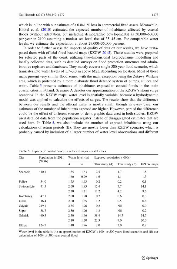
weirs. Table 5 presents estimates of inhabitants exposed to coastal floods in the main
coastal cities in Poland. Scenario A denotes our approximation of the KZGW’s storm surge
scenarios. In the KZGW maps, water level is spatially variable, because a hydrodynamic
model was applied to calculate the effects of surges. The results show that the difference
between our results and the official maps is mostly small, though in every case, our
estimates of the number of inhabitants exposed are higher. However, part of the difference
could be the effect of different sources of demographic data used in both studies. KZGW
used detailed data from the population register instead of disaggregated estimates that are
used here. In Table 5, we also include the number of exposed inhabitants using our
calculations of return periods (B). They are mostly lower than KZGW scenario, which is
probably caused by inclusion of a larger number of water level observations and different
Table 5 Impacts of coastal floods in selected major coastal cities
City Population in 2011(‘000s)
Water level (m) Exposed population (‘000s)
A B This study (A) This study (B) KZGW maps
Szczecin 410.1 1.85 1.63 2.5 1.7 1.8
1.60 0.99 1.6 1.1 1.3
Police 34.0 1.75 1.63 0.2 0.2 0.1
Swinoujscie 41.5 2.60 1.93 15.4 7.7 14.1
2.30 1.21 11.2 4.2 9.6
Kołobrzeg 47.1 2.00 1.98 0.7 0.6 0.3
Ustka 16.4 2.60 1.85 1.2 0.5 0.8
Gdynia 249.1 2.35 1.96 0.2 Nil 0.0
Sopot 38.7 2.50 1.96 1.3 Nil 0.2
Gdansk 460.3 2.50 1.96 38.4 14.7 34.7
2.10 1.20 22.3 7.0 20.0
Elblag 124.7 1.40 1.96 2.0 3.0 0.7
Water level in the table is (A) an approximation of KZGW’s 100- or 500-years flood scenarios and (B) ourcalculation of 100- or 500-year coastal flood
Nat Hazards (2017) 85:1249–1277 1273
123

methodology of return period calculations in that study. In effect, our estimate of the
number of affected inhabitants for a comparable return period is lower.
5 Conclusions
In this paper, we have undertaken a broad analysis of potential impacts of inundation
caused by sea level rise and coastal floods in the Polish coastal zone. Its aim was to
increase the accuracy and level of detail of country-wide risk estimates, covering both
population and economics, compared to currently available studies. This was made pos-
sible by recent developments in the national stock of spatial data. The most important
findings of the study are:
• Impacts of SLR, as well as adaptation costs to SLR, will be much smaller than
indicated in previous studies. 1 m SLR would affect directly 20,000 inhabitants and 9.6
bln PLN of assets (0.6 % of GDP), while the cost of increasing flood defences for full
protection of the population would be 1.9 bln PLN.
• Annualized, adaptation costs and remaining losses would be equivalent of a fraction of
average coastal protection budget (about 0.0025 % of GDP); only in the highest IPCC
projection, the budget would have to be more than doubled by the 2080s.
• Coastal floods will increase substantially in frequency due to sea level rise. Half-meter
SLR will double the number of inhabitants and assets in the 100-year flood zone, while
1 m SLR will more than triple it. Economically optimal flood defences would cost
0.39 % of GDP at current climate conditions, and 0.49–0.67 % of GDP within SLR
scenarios indicated by IPCC.
• Rural population would be proportionately much more exposed than inhabitants in
urban areas. Assets used in agricultural production are the most exposed category
within the range of IPPC projections of SLR. For higher SLR values and coastal floods,
housing comprises the biggest percentage of assets at risk, at about 40 %.
• SLR will have very limited direct impact on the regionally important tourist industry.
However, the beaches and natural reserves which draw the visitors are among the most
vulnerable: more than half of the land in the ?1 m MSL hazard zone is under some
kind of environmental protection.
But again, one should bear in mind that several simplifications have been used in this
study and more research is required, especially on coastal flood scenarios, damage curves,
future climate, population and economic projections. More advanced modelling techniques
that take into account dynamics of storm surges and coastal processes (erosion and sedi-
mentation) are yet to be used in the Polish coastal zone.
Acknowledgments The authors would like to thank the Central Surveying and Cartographic Documenta-tion Center (CODGiK) in Warsaw, Poland, for kindly providing the topographic objects database and digitalelevation models used in this study. Special thanks should be extended to S. N. Jonkman for his commentson the draft of this paper, as well as to the anonymous referees for their detailed suggestions which helped toimprove this paper significantly.
Open Access This article is distributed under the terms of the Creative Commons Attribution 4.0 Inter-national License (http://creativecommons.org/licenses/by/4.0/), which permits unrestricted use, distribution,and reproduction in any medium, provided you give appropriate credit to the original author(s) and thesource, provide a link to the Creative Commons license, and indicate if changes were made.
1274 Nat Hazards (2017) 85:1249–1277
123

References
Apel H, Aronica GT, Kreibich H, Thieken AH (2009) Flood risk analyses—how detailed do we need to be?Nat Hazards 49:79–98. doi:10.1007/s11069-008-9277-8
Bates P, De Roo AP (2000) A simple raster-based model for flood inundation simulation. J Hydrol236:54–77. doi:10.1016/S0022-1694(00)00278-X
Bednarczyk S, Jarzebinska T, Mackiewicz S, Wołoszyn E (2006) Vademecum ochrony przeciw-powodziowej. Krajowy Zarzad Gospodarki Wodnej, Gdansk
Bosello F, Nicholls RJ, Richards J, Roson R, Tol RSJ (2012) Economic impacts of climate change inEurope: sea-level rise. Clim Change 112:63–81. doi:10.1007/s10584-011-0340-1
Breilh JF, Chaumillon E, Bertin X, Gravelle M (2013) Assessment of static flood modeling techniques:application to contrasting marshes flooded during Xynthia (western France). Nat Hazards Earth SystSci 13:1595–1612. doi:10.5194/nhess-13-1595-2013
Cardona OD, van Aalst MK, Birkmann J, Fordham M, McGregor G, Perez R, Pulwarty RS, Schipper ELF,Sinh BT (2012) Determinants of risk: exposure and vulnerability. In: Field CB, Barros V, Stocker TF,Qin D, Dokken DJ, Ebi KL, Mastrandrea MD, Mach KJ, Plattner GK, Allen SK, Tignor M, MidgleyPM (eds) Managing the risks of extreme events and disasters to advance climate change adaptation.Cambridge University Press, Cambridge and New York, pp 65–108
Church JA, White NJ (2011) Sea-level rise from the late 19th to the early 21st century. Surv Geophys32:585–602. doi:10.1007/s10712-011-9119-1
Church JA, Clark PU, Cazenave A, Gregory JM, Jevrejeva S, Levermann A, Merrifield MA, Milne GA,Nerem RS, Nunn PD, Payne AJ, Pfeffer WT, Stammer D, Unnikrishnan AS (2013) Sea level change.In: Stocker TF, Qin D, Plattne GK, Tignor M, Allen SK, Boschung J, Nauels A, Xia Y, Bex V,Midgley PM (eds) Climate change 2013: the physical science basis contribution of working group I tothe fifth assessment report of the intergovernmental panel on climate change. Cambridge UniversityPress, Cambridge and New York, pp 1137–1216
CODGiK (2014) Numeryczne Dane Wysokosciowe. http://www.codgik.gov.pl/index.php/zasob/numeryczne-dane-wysokosciowe.html. Accessed 11 Dec 2014
CODGiK (2016) Baza Danych Obiektow Topograficznych BDOT10k http://www.codgik.gov.pl/index.php/zasob/baza-danych-obiektow-topograficznych.html. Accessed 27 Jul 2016
CSO (2015). http://stat.gov.pl/en/. Accessed 12 Sept 2015Deng J, Zhang WY, Schneider R, Harff J, Dudzinska-Nowak J, Terefenko P, Giza A, Furmanczyk K (2014)
A numerical approach for approximating the historical morphology of wave-dominated coasts—a casestudy of the Pomeranian Bight, southern Baltic Sea. Geomorphology 204:425–443. doi:10.1016/j.geomorph.2013.08.023
Eijgenraam CJJ (2006) Optimal safety standards for dike-ring areas. CPB Netherlands Bureau for EconomicPolicy Analysis Discussion Paper 62
Ekman M (2009) The changing level of the Baltic Sea during 300 years: a clue to understanding the Earth.Summer Institute for Historical Geophysics, Aland Islands
Emschergenossenschaft/Hydrotec (2004) Hochwasser-Aktionsplan Emscher—Methodik der Schadenser-mittlung. http://www.eglv.de/fileadmin/EmscherGenossenschaft/2.3_Flussgebietsmanagement/Karten_Anlage/Methodik_der_Schadensermittlung/methodik_schadensermittlung.pdf. Accessed 12Sept 2015
EU (2007) Directive 2007/60/EC of the European Parliament and of the Council of 23 October 2007 on theassessment and management of flood risks. OJ L 288:27–34
Eurostat (2015). http://epp.eurostat.ec.europa.eu/portal/page/portal/statistics/themes. Accessed 27 Aug 2015Furmanczyk K, Andrzejewski P, Benedyczak R, Bugajny N, Cieszynski Ł, Dudzinska-Nowak J, Giza A,
Paprotny D, Terefenko P, Zawislak T (2014) Recording of selected effects and hazards caused bycurrent and expected storm events in the Baltic Sea coastal zone. J Coast Res Special Issue70:338–342. doi:10.2112/SI70-057.1
Grawe U, Burchard H (2012) Storm surges in the Western Baltic Sea: the present and a possible future. ClimDyn 39:165–183. doi:10.1007/s00382-011-1185-z
Hallegatte S (2012) A framework to investigate the economic growth impact of sea level rise. Environ ResLett 7:015604. doi:10.1088/1748-9326/7/1/015604
Hinkel J, Nicholls RJ, Vafeidis AT, Tol RS, Avagianou T (2010) Assessing risk of and adaptation to sea-level rise in the European Union: an application of DIVA. Mitig Adapt Strateg Glob Change15:703–719. doi:10.1007/s11027-010-9237-y
Hinkel J, Linckea D, Vafeidis AT, Perrettec M, Nicholls RJ, Tol RSJ, Marzeion B, Fettweis X, Ionescu C,Levermann A (2014) Coastal flood damage and adaptation costs under 21st century sea-level rise. ProcNatl Acad Sci USA 111:3292–3297. doi:10.1073/pnas.1222469111
Nat Hazards (2017) 85:1249–1277 1275
123
Huizinga H (2007) Flood damage functions for EU member states. JRC-Institute for Environment andSustainability/HKV Consultants: Lelystad
Hunter J (2010) Estimating sea-level extremes under conditions of uncertain sea-level rise. Clim Change99:331–350. doi:10.1007/s10584-009-9671-6
Jonkman SN, Hillen MM, Nicholls RJ, Kanning W, van Ledden M (2013) Costs of adapting coastaldefences to sea-level rise—new estimates and their implications. J Coast Res 29:1212–1226
Kok M, Huizinga H, Vrouwenvelder A, Barendregt A (2004) Standaardmethode2004—Schade enSlachtoffers als gevolg van overstromingen. DWW-2005-005, RWS Dienst Weg-en Waterbouwkunde
Kron F (2005) Flood risk = hazard * values * vulnerability. Water Int 30(1):58–68. doi:10.1080/02508060508691837
Kummu M, de Moel H, Salvucci G, Viviroli D, Ward PJ, Varis O (2016) Over the hills and further awayfrom coast: global geospatial patterns of human and environment over the 20th–21st centuries. EnvironRes Lett 11(3):034010. doi:10.1088/1748-9326/11/3/034010
KZGW (2011) Raport z wykonania wstepnej oceny ryzyka powodziowego. KZGW, Warszawa. http://www.kzgw.gov.pl/pl/Wstepna-ocena-ryzyka-powodziowego.html. Accessed 10 Feb 2015
KZGW (2015) Informatyczny System Osłony Kraju. http://mapy.isok.gov.pl/imap/. Accessed 10 Feb 2015Łonyszyn P, Terefenko O (2014) Creation of an alternative season based on sustainable tourism as an
opportunity for Baltic Sea Region. J Coast Res Special Issue 70:454–459. doi:10.2112/SI70-077.1Merz B, Kreibich H, Thieken A, Schmidtke R (2004) Estimation uncertainty of direct monetary flood
damage to buildings. Nat Hazards Earth Syst Sci 4:153–163. doi:10.5194/nhess-4-153-2004Ministry of Treasury (2012) Sprawozdanie o stanie mienia Skarbu Panstwa. Warsaw. http://bip.msp.gov.pl/
download/1/5554/Sprawozdanie2011.pdf. Accessed 10 Feb 2015Mokrech M, Kebede AS, Nicholls RJ, Wimmer F, Feyen L (2015) An integrated approach for assessing
flood impacts due to future climate and socio-economic conditions and the scope of adaptation inEurope. Clim Change 128:245–260. doi:10.1007/s10584-014-1298-62015
Muis S, Guneralp B, Jongman B, Aerts JCJH, Ward PJ (2015) Flood risk and adaptation strategies underclimate change and urban expansion: a probabilistic analysis using global data. Sci Total Environ538:445–457. doi:10.1016/j.scitotenv.2015.08.068
Nicholls RJ, Klein RJT (2005) Climate change and coastal management on Europe’s coast. In: Vermaat JE,Bouwer L, Turner K, Salomons W (eds) Managing European coasts: past, present and future, envi-ronmental science monograph series. Springer, Berlin, pp 199–226
Nicholls RJ, Mimura N (1998) Regional issues raised by sea-level rise and their policy implications. ClimRes 11:5–18
NOAA (2016) Sea level rise maps. http://www.star.nesdis.noaa.gov/sod/lsa/SeaLevelRise/LSA_SLR_maps.php. Accessed 27 Jul 2016
Paprotny D (2014) Trends in storm surge probability of occurrence along the Polish Baltic Sea coast. arXiv:1410.2547
Peltier WR, Argus DF, Drummond R (2015) Space geodesy constrains ice-age terminal deglaciation: theglobal ICE-6G_C (VM5a) model. J Geophys Res Solid Earth 120:450–487. doi:10.1002/2014JB011176
Permanent Service for Mean Sea Level (2015). http://www.psmsl.org/data/obtaining/map.html. Accessed 8Jan 2015
Pfeffer WT, Harper JT, O’Neel S (2008) Kinematic constraints on glacier contributions to 21st century sealevel rise. Science 321:1340–1343. doi:10.1126/science.1159099
Piketty T, Zucman G (2014) Capital is back: wealth-income ratios in rich countries, 1700–2010. Q J Econ129:1155–1210. doi:10.1093/qje/qju018
Pluijm M, Toms G, Zeidler RB, van Urk A, Misdorp R (1992) Vulnerability assessment to accelerated sealevel rise: case study Poland. Ministry of Transport, Public Works and Water Management, The Hague
Poulter B, Halpin PN (2008) Raster modelling of coastal flooding from sea-level rise. Int J Geogr Inf Sci22:167–182. doi:10.1080/13658810701371858
Pruszak Z, Zawadzka E (2005) Vulnerability of Poland’s coast to sea-level rise. Coast Eng J 47:131–155.doi:10.1142/S0578563405001197
Pruszak Z, Zawadzka E (2008) Potential implications of sea-level rise for Poland. J Coast Res 24:410–422.doi:10.2112/07A-0014.1
Rahmstorf S (2007) Sea-level rise a semi-empirical approach to projecting future. Science 315:368–370.doi:10.1126/science.1135456
Richter A, Groh A, Dietrich R (2012) Geodetic observation of sea-level change and crustal deformation inthe Baltic Sea region. Phys Chem Earth 53–54:43–53. doi:10.1016/j.pce.2011.04.011
1276 Nat Hazards (2017) 85:1249–1277
123

Rotnicki K, Borowka RK (1991) Impact of a future sea level rise in the Polish Baltic coastal zone. EPAInternational Sea Level Rise Studies Project Report. Division of Coastal and Environmental Studies.Rutgers University Institute of Coastal and Marine Sciences, New Brunswick
Rotnicki K, Borowka RK, Devine N (1995) Accelerated sea level rise as a threat to the Polish CoastalZone—quantification of risk. J Coast Res Special Issue 22:111–135
Rotzoll K, Fletcher CH (2013) Assessment of groundwater inundation as a consequence of sea-level rise.Nat Clim Change 3:477–481. doi:10.1038/nclimate1725
Statistisches Bundesamt (2015) Bau- und Immobilienpreise. https://www.destatis.de/DE/ZahlenFakten/GesamtwirtschaftUmwelt/Preise/BauImmobilienpreise/BauImmobilienpreise.html. Accessed 21 Jan2015
Tomczak A (1995) Geological structure and Holocene evolution of the Polish coastal zone. J Coast ResSpecial Issue 22:16–31
Urbanski J (2012) GIS w badaniach przyrodniczych. University of Gdansk, GdanskVan Dantzig D (1956) Economic decision problems for flood prevention. Econometrica 24:276–287Vousdoukas MI, Voukouvalas E, Annunziato A, Giardino A, Feyen L (2016) Projections of extreme storm
surge levels along Europe. Clim Dyn. doi:10.1007/s00382-016-3019-5Webster TL (2010) Flood risk mapping using LiDAR for Annapolis Royal, Nova Scotia, Canada. Remote
Sens 2:2060–2082. doi:10.3390/rs2092060Wisniewski B, Kowalewska-Kalkowska H (2007) Water level fluctuations in the Odra River mouth area in
relation to passages of deep low-pressure systems. Oceanol Hydrobiol Stud 36:69–82. doi:10.2478/v10009-007-0009-2
Wisniewski B, Wolski T (2009) Katalogi wezbran i obni _zen sztormowych poziomow morza oraz ekstre-malne poziomy wod na polskim wybrze _zu. Maritime University of Szczecin, Szczecin
Wisniewski B, Wolski T, Musielak S (2011) A long-term trend and temporal fluctuations of the sea level atthe Polish Baltic coast. Oceanol Hydrobiol Stud 40:96–107. doi:10.2478/s13545-011-0020-9
Wolski T, Wisniewski B, Giza A, Kowalewska-Kalkowska H, Boman H, Grabbi-Kaiv S, Hammarklint T,Holfort J, Lydeikait _e Z (2014) Extreme sea levels at selected stations on the Baltic Sea coast.Oceanologia 56:259–290. doi:10.5697/oc.56-2.259
Wroblewski A (1994) Analysis and forecast of long-term sea level changes along the Polish Baltic Seacoast. Part II. Annual mean sea levels—forecast to the year 2100. Ocealonogia 36:107–120
Xu S, Huang W (2013) Effects of sea level rise on frequency analysis of 1 % annual maximum water levelsin the coast of Florida. Ocean Eng 71:96–102. doi:10.1016/j.oceaneng.2013.01.013
Zeidler RB (1997) Climate change vulnerability and response strategies for the coastal zone of Poland. ClimChange 36:151–173. doi:10.1023/A:1005394909182
Nat Hazards (2017) 85:1249–1277 1277
123