New Evidence on Cyclical and Structural Sources of Unemployment

Jinzhu Chen, Prakash Kannan, Prakash Loungani and

Bharat Trehan

WP/11/106

© 2011 International Monetary Fund WP/11/106

IMF Working Paper

Research Department

New Evidence on Cyclical and Structural Sources of Unemployment

Prepared by Jinzhu Chen, Prakash Kannan, Prakash Loungani and Bharat Trehan*

May 2011

Abstract

We provide cross-country evidence on the relative importance of cyclical and structural factors in explaining unemployment, including the sharp rise in U.S. long-term unemployment during the Great Recession of 2007-09. About 75% of the forecast error variance of unemployment is accounted for by cyclical factors—real GDP changes (―Okun‘s Law‖), monetary and fiscal policies, and the uncertainty effects emphasized by Bloom (2009). Structural factors, which we measure using the dispersion of industry-level stock returns, account for the remaining 25 percent. For U.S. long-term unemployment the split between cyclical and structural factors is closer to 60-40, including during the Great Recession.

JEL Classification Numbers: E24, E32, E44, J6, J64 Keywords: unemployment; structural unemployment; stock markets; uncertainty Author‘s E-Mail Addresses: chen25@fas.harvard.edu; pkannan@imf.org; ploungani@imf.org and Bharat.Trehan@sf.frb.org

* We thank Larry Ball and David Romer for extensive comments on earlier versions of this work. We also thank Daniel Aaranson, Menzie Chinn, Robert Hall, Joao Jalles, Daniel Leigh, Akito Matsumoto, Gian Maria Milesi-Ferretti, Romain Ranciere, Ellen Rissman, Jorge Roldos, Kenichi Ueda, Ken West and seminar participants at the University of Wisconsin, Madison (Conference on ―Long-Term Unemployment‖ organized by Menzie Chinn and Mark Copelovitch), IMF, Paris School of Economics and the Midwest Economic Association meetings in Chicago.

This Working Paper should not be reported as representing the views of the IMF.

The views expressed in this Working Paper are those of the author(s) and do not necessarily represent those of the IMF or IMF policy. Working Papers describe research in progress by the author(s) and are published to elicit comments and to further debate.

Contents Pages

I. Introduction ......................................................................................................... 3 II. Measuring Sectoral Shifts ................................................................................... 6 III. Candidate Explanations for Changes Duration ................................................... 9 IV. VARs Estimated on U.S. Data ......................................................................... 11

A. The Effects of Sectoral Shocks ................................................................... 12 B. Sectoral Shocks and Long-Term Unemployment during the Great

Recession .................................................................................................... 13 C. Structural vs. Cyclical Movements in Unemployment ............................... 14

V. Sectoral Shocks Versus Uncertainty ................................................................. 15 VI. A VAR Estimated on International Data ......................................................... 17 VII. Conclusion ........................................................................................................ 20 Figures

1. Average Duration of Unemployment (Weeks) ......................................... 22 2. Duration of Unemployment (Percent of Labor Force) .............................. 23 3. Change in Unemployment Rate 2007-09 (Percent) .................................. 24 4. Stock Market Returns Dispersion Index (6-month moving average) ....... 25 5. Impulse-Response Figures for Unemployment (Univariate Model) ......... 26 6. Impulse-Response Figures for Long-Term Unemployment (Univariate

Model) ....................................................................................................... 27 7. Impulse-Response Figures for Unemployment (VAR model).................. 28 8. Impulse-Response Figures for Long-Term Unemployment (VAR model)29 9. Variance of Unemployment ...................................................................... 30 10. Decomposition of Long-Term Unemployment During the Great

Recession................................................................................................... 31 11. Estimates of Structural Unemployment .................................................... 32 12. Dispersion Index and the Uncertainty Index ............................................. 33 13. Comparing Unemployment Responses to Dispersion and Uncertainty

Shocks ....................................................................................................... 34 14. Variance of Unemployment ...................................................................... 35 15. Impulse-Response Figures for Unemployment (Panel VAR Model) ....... 36

Tables

1. Forecast-error Variance Decomposition for the Unemployment Rate ................ 37 2. Forecast-error Variance Decomposition for the Long-Term Unemployment

Rate ...................................................................................................................... 37 3. Forecast-error Variance Decomposition for the Long-Term Unemployment

Rate ...................................................................................................................... 37 4. Forecast-error Variance Decomposition for the Unemployment Rate –

International Panel ............................................................................................... 37 References .................................................................................................................... 38

3

I. INTRODUCTION

Are persistent increases in unemployment cyclical or structural? The question is

timely and timeless. It is timely because the sharp run-up in U.S. unemployment rates since

2007 has triggered a debate on the contribution of structural factors; it is timeless because

nearly every persistent increase in unemployment over the past 100 years has been marked

by a debate of this kind. Krugman (2010) states that the present ―high unemployment in

America is the result of inadequate demand—full stop‖, whereas Kocherlakota (2010) asserts

that ―firms have jobs, but can't find appropriate workers. The workers want to work, but

can't find appropriate jobs.‖

The jobless recovery following the 2001 U.S. recession led some observers, notably

Groshen and Potter (2003), to assign a significant role to structural factors, while others took

a more skeptical view (e.g. Aaronson, Rissman and Sullivan, 2004). Going further back in

time, the persistent unemployment of the Great Depression was also attributed by some to ―a

great shortage of labor of certain kinds‖ (Clague 1935). Likewise, the causes of the high

unemployment in Great Britain during the interwar years were a matter of intense debate

then and to this day (see Benjamin and Kochin, 1979; Loungani, 1991; Brainard, 1992;

Nason and Vahey, 2006).

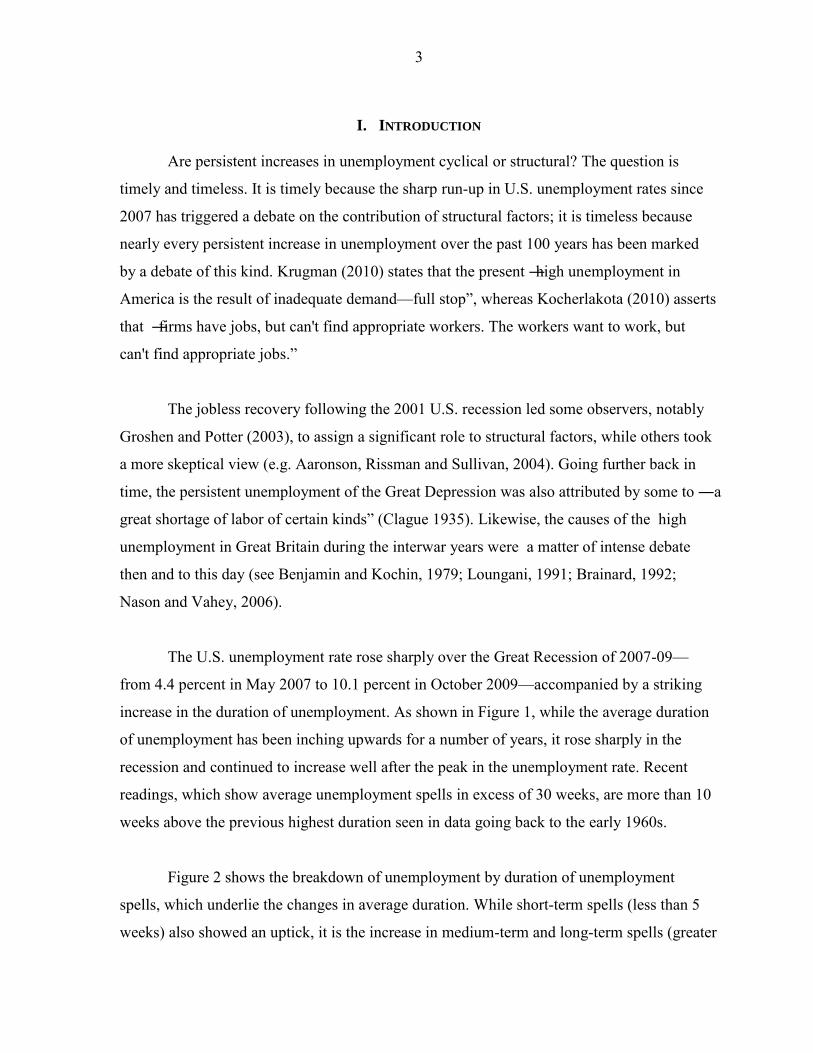
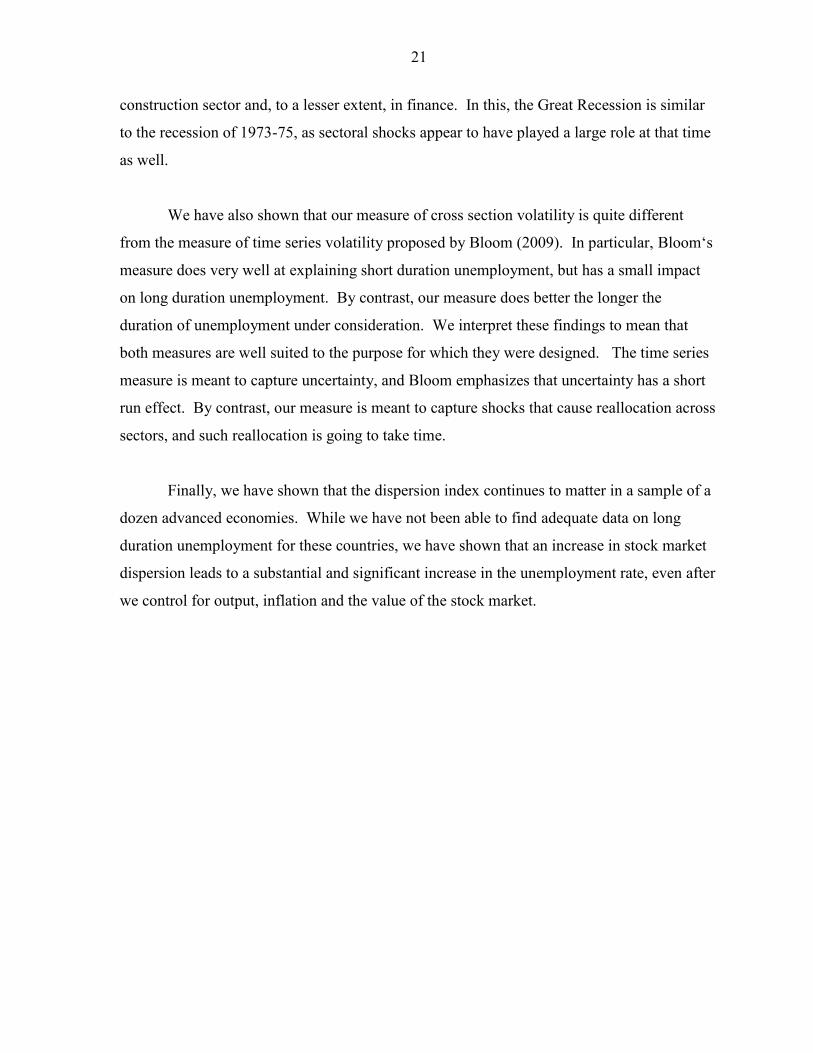
The U.S. unemployment rate rose sharply over the Great Recession of 2007-09—

from 4.4 percent in May 2007 to 10.1 percent in October 2009—accompanied by a striking

increase in the duration of unemployment. As shown in Figure 1, while the average duration

of unemployment has been inching upwards for a number of years, it rose sharply in the

recession and continued to increase well after the peak in the unemployment rate. Recent

readings, which show average unemployment spells in excess of 30 weeks, are more than 10

weeks above the previous highest duration seen in data going back to the early 1960s.

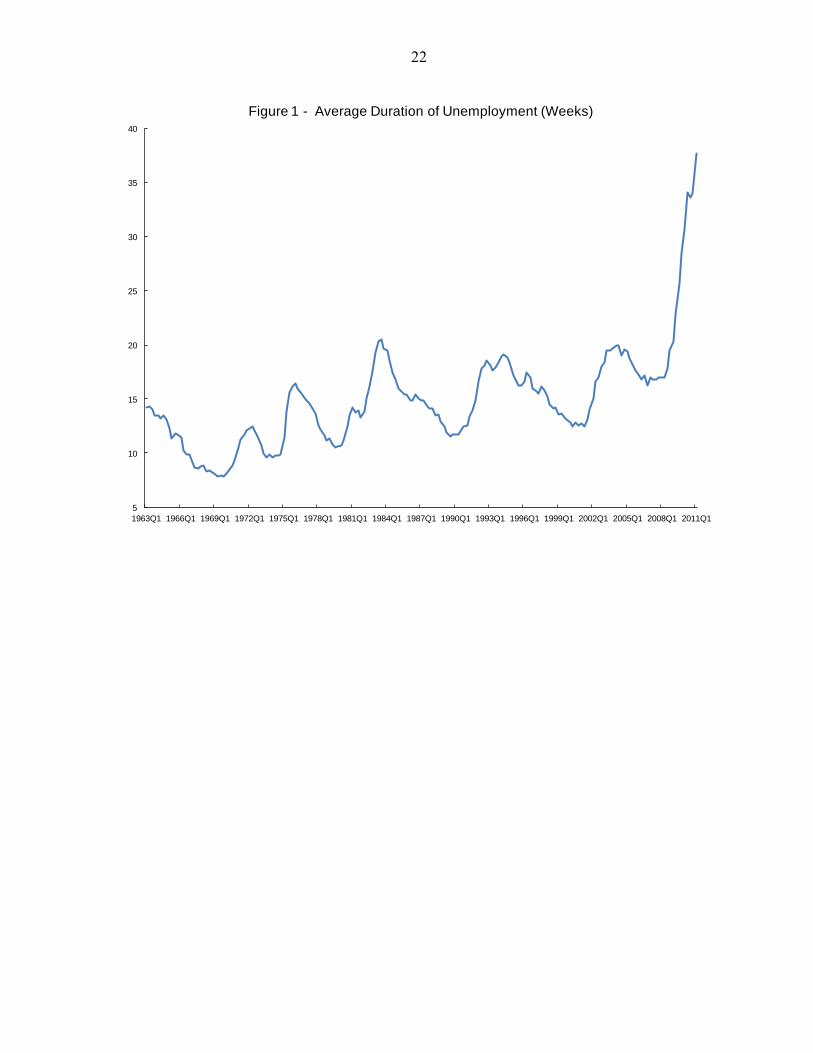
Figure 2 shows the breakdown of unemployment by duration of unemployment

spells, which underlie the changes in average duration. While short-term spells (less than 5

weeks) also showed an uptick, it is the increase in medium-term and long-term spells (greater

4

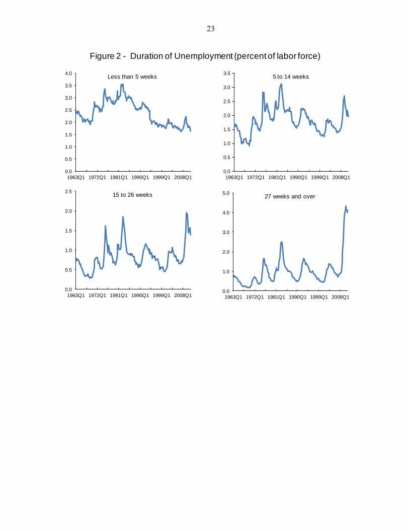
than 27 weeks) that is particularly alarming. In Figure 3, the increase in U.S. unemployment

rates during the Great Recession is compared with that in 12 other industrialized countries.

While there have been increases elsewhere as well, there is also considerable heterogeneity in

unemployment outcomes.

The severity and persistence of output declines during the Great Recession are clearly

the dominant factor in pushing up U.S. unemployment (Elsby, Hobijn and Sahin, 2010) and

in explaining the cross-country differences in unemployment (IMF 2010). But studies by

Kirkegaard (2009) and Sahin, Song, Topa and Violante (2011) suggest that structural factors

may have played a role as well. Kirkegaard (2009) extends the analysis of Groshen and

Potter to study structural and cyclical employment trends in the U.S. economy during the

Great Recession. He finds that there has been a sharp increase in ―the relative employment

weight of industries undergoing structural change in the current cycle‖, which he concludes

―can be expected to increase the necessity for unemployed Americans to take new jobs in

industries different from the ones in which they were previously employed.‖

Sahin, Song, Topa and Violante (2011) measure mismatch in the U.S. and U.K. labor

market, defined as the distance between the observed allocation of unemployment across

sectors and the allocation that would prevail under costless mobility. Using data on

unemployment and vacancies they find that between 0.8 and 1.4 percentage points of the

increase in U.S. unemployment during the Great Recession can be attributed to mismatch.

This corresponds to between 20% and 25% of the observed increase in unemployment. They

also find industrial and occupational mismatches, rather than geographic mismatch, are the

sources of the increased unemployment. For the U.K. they find that 0.8 percent of the

increased unemployment—which corresponds to a third of the increase—during the Great

Recession was due to mismatch.2

2 Barnichon and Figura (2011) study the determinants of the U.S. economy‘s matching efficiency, i.e.,

the number of job matches formed each period conditional on unemployment and vacancies. They find that until 2006, most of the changes in matching efficiency could be explained by changes in the composition of the unemployed (for instance, the relative prevalence of workers on temporary vs. permanent layoffs). Since 2006, however, composition has played a much diminished role relative to the role of ―dispersion in labor market

(continued)

5

Estevao and Tsounta (2011) find that ―increases in skill mismatches in [U.S.] states

with worse housing market conditions … are associated with even higher unemployment

rates, after controlling for all cyclical factors.‖ They suggest that this could be because ―bad

local housing conditions may slow the exodus of jobless individuals from a depressed area,

thus raising equilibrium unemployment rates.‖ They estimate that the combined impact of

skill mismatches and higher foreclosure rates might have raised the U.S. natural rate of

unemployment by about 1½ percentage points since 2007.

This paper provides further evidence on the role of structural factors in accounting for

the rise in U.S. unemployment (particularly long-term unemployment), as well as the rise in

unemployment in other industrialized countries. Our measure of the intensity of structural

shocks implements a conjecture by Black (1987) that periods of greater cross-industry

dispersion in stock returns should be followed by increases in unemployment. The idea, as

expressed in more recent work by Beaudry and Portier (2004) is that ―stock prices are likely

a good variable for capturing any changes in agents expectations about future economic

conditions‖. Hence the cross-industry dispersion of stock returns provides an ―early signal of

shocks that affect sectors differently, and puts more weight on shocks that investors expect to

be permanent‖ (Black 1995). This latter point is important because it is presumably

permanent shocks that motivate reallocation of labor across industries.

While explaining developments in unemployment during the Great Recession is an

important motivation for our work, the results should be of broader interest for a couple of

reasons. First, as noted above, the relative importance on cyclical and structural factors has

long been a source of debate, both in the U.S. and in other countries. While the stock market

dispersion measure has been used before (Loungani, Rush and Tave, 1990; Brainard and

Cutler, 1993; Loungani and Trehan, 1997), the work in the present paper represents a

significant out-of-sample test of that earlier work. With the extension of the data set to the

conditions, the fact that tight labor markets coexist with slack ones.‖ They estimate that in the 2008-2009 recession, the decline in aggregate matching efficiency added 1 ½ percentage points to the unemployment rate.

6

present, it now includes the recessions of 2001 and 2007-2009. We also test if, as seems

reasonable, the impact of structural shocks is greater for long-term unemployment than for

short-term unemployment. We also extend our results to a new data set, the sample of 12

developed economies listed earlier in Figure 3. Consistent with the earlier studies, the stock

market dispersion measure accounts for a significant part of U.S. unemployment fluctuations

after controlling for aggregate factors. Moreover, the dispersion index exerts a much greater

impact of long-term unemployment than on short-term unemployment. In the cross-country

work, we gain find that the unemployment rate increases significantly following an increase

in stock market dispersion, after controlling for aggregate factors.

Second, while not a direct test, our evidence provides support for recent theoretical

work that assigns an important role to structural shocks. Phelan and Trejos (2000) show that

permanent changes in sectoral composition can lead to aggregate downturns in a calibrated

job creation/job destruction model of the U.S. labor market. Bloom (2009) and Bloom,

Floetotto and Jaimovich (2009) propose ―uncertainty shocks‖ as a source of aggregate

fluctuations. Surges in uncertainty give firms pause in their hiring and investment decisions,

leading to temporarily low factor usage. Bloom uses stock market volatility (in the time

dimension) as an empirical measure of uncertainty in the economy. Consistent with his

argument that an increase in uncertainty has a temporary negative effect on the economy, we

find that an increase in the volatility index raises short duration unemployment but has

almost no effect on long duration unemployment. Our stock market dispersion index has a

larger effect on aggregate unemployment than Bloom‘s uncertainty index and, as noted, its

impact increases significantly as we move from short to long duration unemployment.

Section II describes the construction of the stock market dispersion index. The next

three sections present our evidence for the U.S economy. In section III, we use univariate

regressions as in Romer and Romer (2003) to see how aggregate factors affect overall

unemployment and long-term unemployment. Complementing this evidence, results from a

VAR model are presented in section IV. In section V the VAR model is augmented to

provide a comparison of the relative performance of the stock market dispersion index and

7

Bloom‘s uncertainty index. Cross-country evidence from a panel VAR is provided in section

VI.

II. MEASURING SECTORAL SHIFTS

The amount of labor reallocation that an economy has to carry out can change

significantly over time. Some periods may be marked by relatively homogeneous growth in

labor demand across sectors, whereas others may be characterized by shifts in the

composition of labor demand. While beneficial in the long run, the reallocation of labor in

response to sectoral shifts imposes short-run costs in the form of increases in unemployment.

The greater the divergence in the fortunes of different industries, the more resources must be

moved, and the larger will be the resulting increase in unemployment.

While these ideas are fairly intuitive, constructing a satisfactory measure of sectoral

shifts poses an empirical challenge for a couple of reasons. First, as stated by Barro (1986),

shocks to the expected profitability of an industry can arrive from ―many—mostly

unobservable—disturbances to technology and preferences [that] motivate reallocations of

resources across sectors.‖ Second, Davis (1985) points out that ―allocative disturbances from

any particular source are likely to occur rather infrequently over available sample sizes,‖

[italics ours] which makes it difficult to incorporate variables explicitly that capture the

effects of sectoral shifts into an aggregate unemployment equation.

These considerations motivated Lilien‘s (1982) construction of a cross-industry

employment dispersion index to proxy for the intersectoral flow of labor in response to

allocative shocks. Lilien argued that frictions associated with the reallocation of labor across

sectors of the economy accounted for as much as half of all fluctuations in unemployment.

Many researchers, most notably Abraham and Katz (1986), however, have questioned

Lilien‘s use of employment dispersion as a measure of labor reallocation. Their basic point is

that movements in employment dispersion may simply be reflecting the well-known fact that

the business cycle has non-neutral effects across industries. The increase in the dispersion of

employment growth rates could reflect not increased labor reallocation, but simply the

uneven impact of aggregate demand shocks on temporary layoffs in different industries.

8

Under certain conditions—for instance, if cyclically responsive industries have low trend

growth rates of employment—aggregate demand shocks also can lead to a positive

correlation between the dispersion index and aggregate unemployment. Hence there is an

observational equivalence between the predictions of the sectoral shifts hypothesis and the

more traditional ―aggregate demand hypothesis.‖ Though Lilien‘s paper inspired a significant

amount of follow-up work, the debate over the relative importance of sectoral shifts and

aggregate shocks in unemployment fluctuations remains unresolved—see Gallipoli and

Pelloni (2008) for a comprehensive critical review of the literature.

Loungani, Rush, and Tave (1990) and Brainard and Cutler (1993) attempt to

circumvent these problems by constructing an index based on stock prices. Assuming that

stock markets are efficient, so that shocks to the expected profitability of an industry are

reflected in its stock market return, and assuming that these shocks are followed by changes

in that industry‘s use of inputs such as labor, their hypothesis is that the dispersion of stock

returns across industries can be used as a proxy for shocks to the desired allocation of labor,

i.e., as a measure of sectoral shifts. For instance, the arrival of positive news regarding the

relative profitability of a particular industry is likely to be followed by an increase in stock

price dispersion. In the long run, this news is likely to shift the economy‘s output mix

towards the affected industry. This will necessitate a reallocation of resources, and the

unemployment rate will rise as part of this process of reallocation of labor across sectors.

Thus, an increase in stock price dispersion will be followed by an increase in the

unemployment rate.

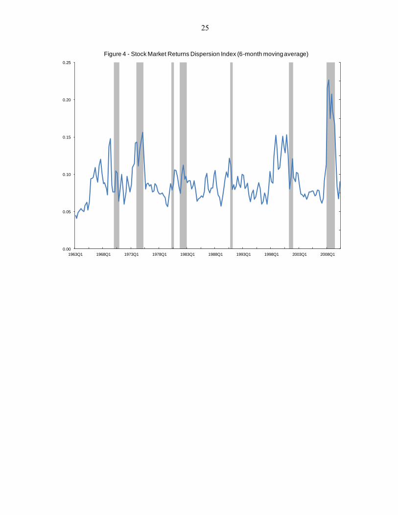
For this paper, we update the stock market index used in these earlier studies. The

basic data consist of Standard and Poor‘s indexes of industry stock prices. There are over 50

industries, and they provide comprehensive coverage of manufacturing as well as

nonmanufacturing sectors of the economy. The sectoral shifts index is defined as

2/1

1

2

n

i

titit RRWDispersion (1)

9

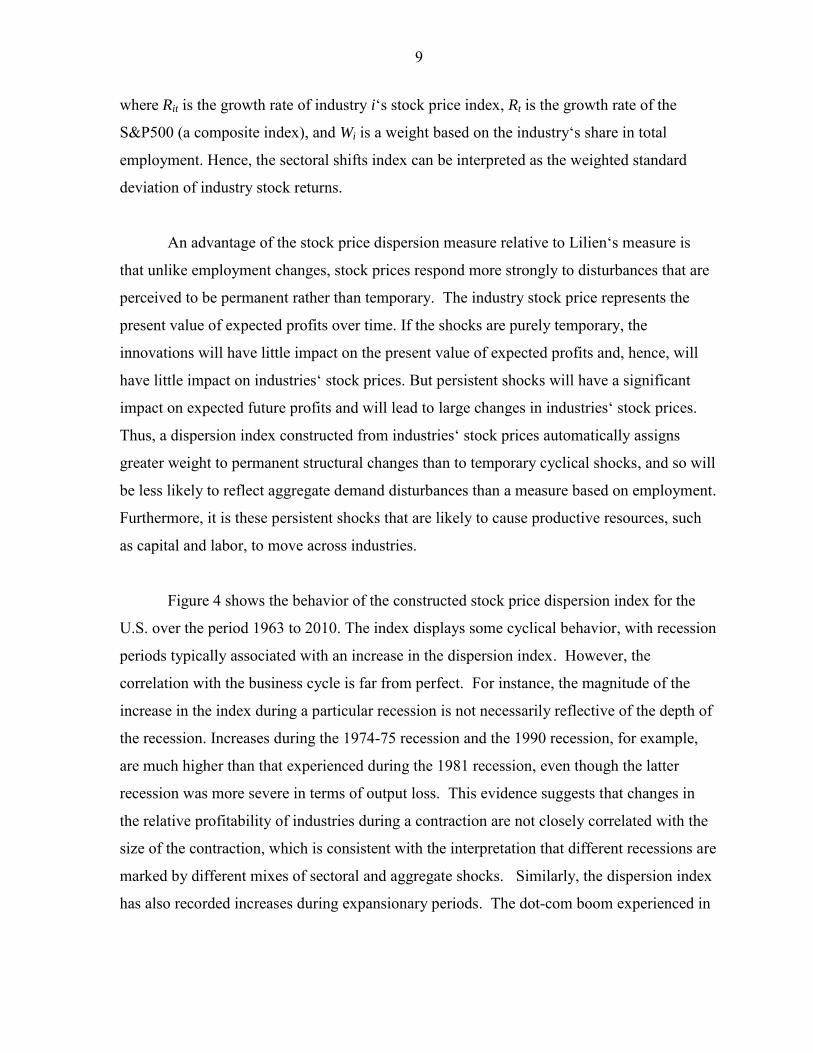
where Rit is the growth rate of industry i‘s stock price index, Rt is the growth rate of the

S&P500 (a composite index), and Wi is a weight based on the industry‘s share in total

employment. Hence, the sectoral shifts index can be interpreted as the weighted standard

deviation of industry stock returns.

An advantage of the stock price dispersion measure relative to Lilien‘s measure is

that unlike employment changes, stock prices respond more strongly to disturbances that are

perceived to be permanent rather than temporary. The industry stock price represents the

present value of expected profits over time. If the shocks are purely temporary, the

innovations will have little impact on the present value of expected profits and, hence, will

have little impact on industries‘ stock prices. But persistent shocks will have a significant

impact on expected future profits and will lead to large changes in industries‘ stock prices.

Thus, a dispersion index constructed from industries‘ stock prices automatically assigns

greater weight to permanent structural changes than to temporary cyclical shocks, and so will

be less likely to reflect aggregate demand disturbances than a measure based on employment.

Furthermore, it is these persistent shocks that are likely to cause productive resources, such

as capital and labor, to move across industries.

Figure 4 shows the behavior of the constructed stock price dispersion index for the

U.S. over the period 1963 to 2010. The index displays some cyclical behavior, with recession

periods typically associated with an increase in the dispersion index. However, the

correlation with the business cycle is far from perfect. For instance, the magnitude of the

increase in the index during a particular recession is not necessarily reflective of the depth of

the recession. Increases during the 1974-75 recession and the 1990 recession, for example,

are much higher than that experienced during the 1981 recession, even though the latter

recession was more severe in terms of output loss. This evidence suggests that changes in

the relative profitability of industries during a contraction are not closely correlated with the

size of the contraction, which is consistent with the interpretation that different recessions are

marked by different mixes of sectoral and aggregate shocks. Similarly, the dispersion index

has also recorded increases during expansionary periods. The dot-com boom experienced in

10

the late 1990s provides a clear example, as stock prices in the information, technology, and

communication sectors experienced much more rapid gains than the market average.

III. CANDIDATE EXPLANATIONS FOR CHANGES IN DURATION

The behavior of the unemployment rate can potentially be influenced by a variety of

factors, both cyclical as well as structural, not all of which can be simultaneously included in

a moderately sized VAR. Accordingly, in this section we compare the effects of the

dispersion index on unemployment rates (of different durations) with the effects of other key

macroeconomic variables, using a single-equation framework similar to Romer and Romer

(2003) and Cerra and Saxena (2008). Specifically, we regress changes in the unemployment

rate (ΔU) on its own lags as well as lagged values of the various ―shocks‖. The lagged values

allow for delays in the impact of the shocks on unemployment.3 The estimated equation is:

t

i

it

i

itt ShockUU

4

1

4

1 (2)

Four candidate shocks are evaluated using this framework. The first two are monetary

and fiscal (tax rate) policy shocks, as identified by Romer and Romer (2003, 2010). Both

these shocks are constructed so as to be exogenous to changes in output through the use of

narrative records of the Federal Reserve Open Market Committee meetings, presidential

speeches and Congressional reports. The third shock examined is related to oil prices, and is

simply measured as the percentage change in the real price of oil. Finally, we look at the

effect of changes in the stock price dispersion index. For each of these shocks, standard

errors for the impulse response functions are estimated using a bootstrap method.4

3 A lag length of 4 quarters was found to be optimal.

4 Specifically, 500 pseudo-coefficients are drawn from a multivariate normal distribution based on the estimates of the mean and variance-covariance matrix of the regression coefficient vector.

11

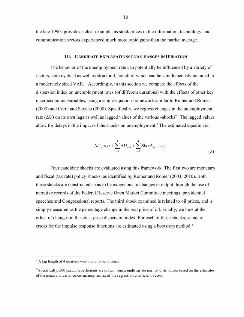
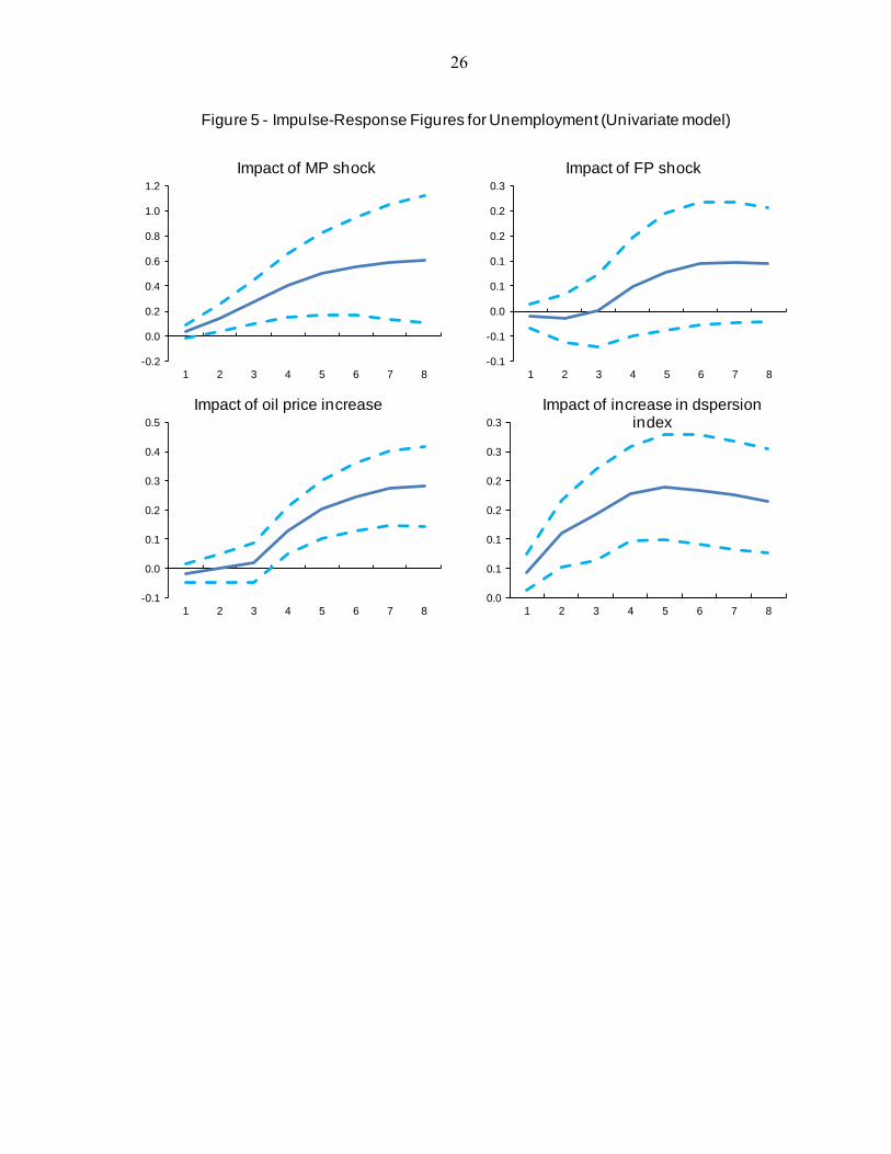
The impact of a one standard-deviation change in the various shocks on the level of

the unemployment rate is shown in Figure 5. The unemployment rate increases following

each shock, though the magnitude and significance of the responses vary across shocks. The

response of unemployment to a monetary policy tightening is particularly large and

persistent. A one standard deviation shock to monetary policy results in an increase in the

unemployment rate of about 0.6 percent after 2 years. Shocks to fiscal policy, on the other

hand, are small and insignificant. In contrast, increases in the real price of oil are associated

with increases in the unemployment rate, with the peak impact occurring after 2 years.

Finally, increases in the dispersion index are associated with a positive and significant

change in the unemployment rate. A 1 standard deviation increase in the index results in an

increase in the unemployment rate of about 0.2 percent after a year and a half.

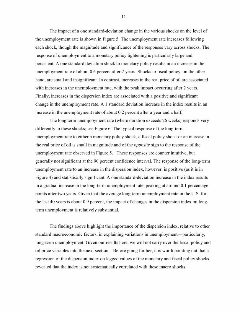
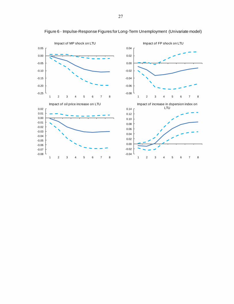
The long term unemployment rate (where duration exceeds 26 weeks) responds very

differently to these shocks; see Figure 6. The typical response of the long-term

unemployment rate to either a monetary policy shock, a fiscal policy shock or an increase in

the real price of oil is small in magnitude and of the opposite sign to the response of the

unemployment rate observed in Figure 5. These responses are counter intuitive, but

generally not significant at the 90 percent confidence interval. The response of the long-term

unemployment rate to an increase in the dispersion index, however, is positive (as it is in

Figure 4) and statistically significant. A one standard-deviation increase in the index results

in a gradual increase in the long-term unemployment rate, peaking at around 0.1 percentage

points after two years. Given that the average long-term unemployment rate in the U.S. for

the last 40 years is about 0.9 percent, the impact of changes in the dispersion index on long-

term unemployment is relatively substantial.

The findings above highlight the importance of the dispersion index, relative to other

standard macroeconomic factors, in explaining variations in unemployment—particularly,

long-term unemployment. Given our results here, we will not carry over the fiscal policy and

oil price variables into the next section. Before going further, it is worth pointing out that a

regression of the dispersion index on lagged values of the monetary and fiscal policy shocks

revealed that the index is not systematically correlated with these macro shocks.

12

IV. VARS ESTIMATED ON U.S. DATA

In this section, we present the results from a VAR estimated on quarterly data from

1963:Q1 to 2010:Q2. The baseline model contains six variables, including the stock market

dispersion index and the unemployment rate. The other variables are: real GDP growth,

inflation, the federal funds rate, and the growth rate of the S&P500 index. The inclusion of

real GDP controls for the stage of the business cycle; it also means that our model allows for

a version of ―Okun‘s Law.‖ The variable measuring returns on the S&P500 index is included

to rule out the possibility that the dispersion index explains unemployment because it is

mimicking the behavior of the aggregate stock market. Finally, following Bernanke and

Blinder (1992), the fed funds rate is included as a measure of monetary policy. The system is

identified following the standard recursive ordering procedure. To avoid exaggerating the

role of the dispersion index, we place it last in the estimation ordering. The other variables in

the system are ordered as follows: GDP growth is placed first, followed by on the growth rate

of the S&P 500, the unemployment rate, inflation and the fed funds rate. A lag length of 6

quarters was found to be optimal based on the Bayesian Information Criterion.

A. The Effects of Sectoral Shocks

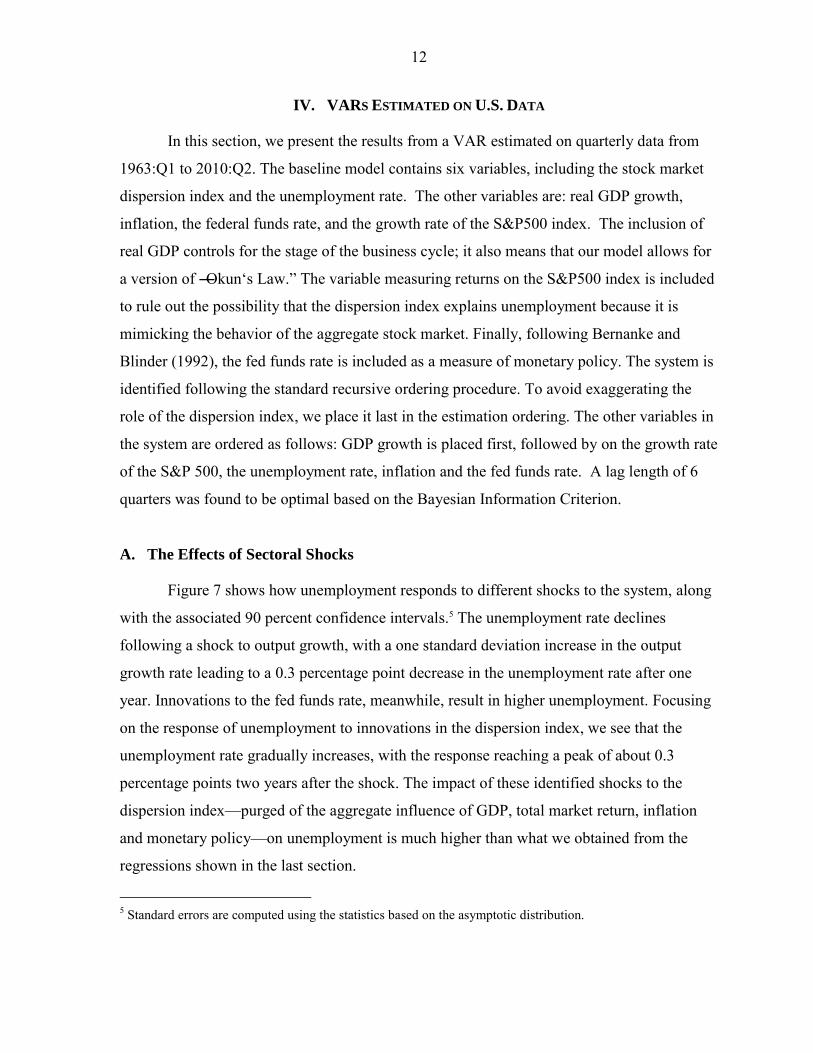
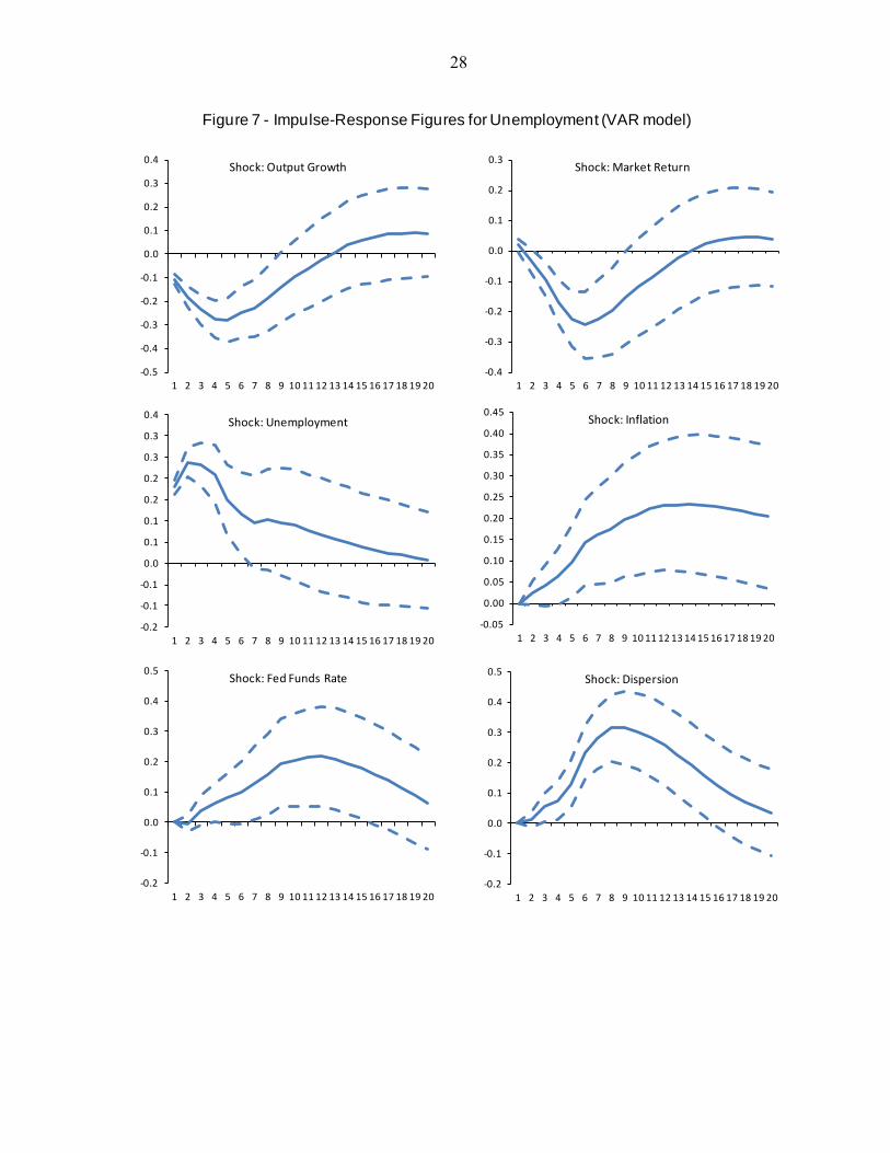
Figure 7 shows how unemployment responds to different shocks to the system, along

with the associated 90 percent confidence intervals.5 The unemployment rate declines

following a shock to output growth, with a one standard deviation increase in the output

growth rate leading to a 0.3 percentage point decrease in the unemployment rate after one

year. Innovations to the fed funds rate, meanwhile, result in higher unemployment. Focusing

on the response of unemployment to innovations in the dispersion index, we see that the

unemployment rate gradually increases, with the response reaching a peak of about 0.3

percentage points two years after the shock. The impact of these identified shocks to the

dispersion index—purged of the aggregate influence of GDP, total market return, inflation

and monetary policy—on unemployment is much higher than what we obtained from the

regressions shown in the last section.

5 Standard errors are computed using the statistics based on the asymptotic distribution.

13

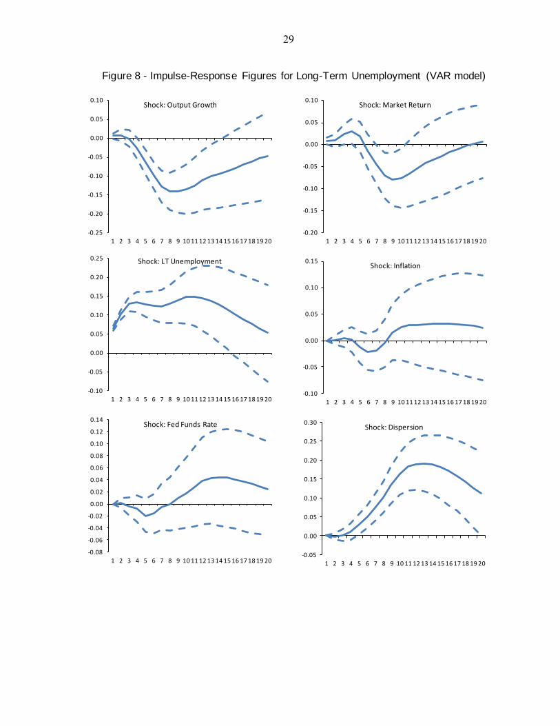
The long-term unemployment rate (Figure 8) shows a hump shaped response to

innovations in the dispersion index, just as the overall unemployment rate (Figure 7).

However, long-term unemployment reacts more gradually, reaching its peak only three years

after the shock. The magnitude of the peak impact is again higher than what was found in the

previous section. Long-term unemployment declines in response to output growth

innovations, though just as with regards to dispersion shocks, the response is more delayed

relative to the response of the overall unemployment rate. Long-term unemployment

eventually increases following a shock to monetary policy, although the magnitude of the

response is insignificant at the 90-percent confidence level.

A decomposition of the variance of unemployment forecast errors provides further

evidence as to the importance of the dispersion index in explaining unemployment

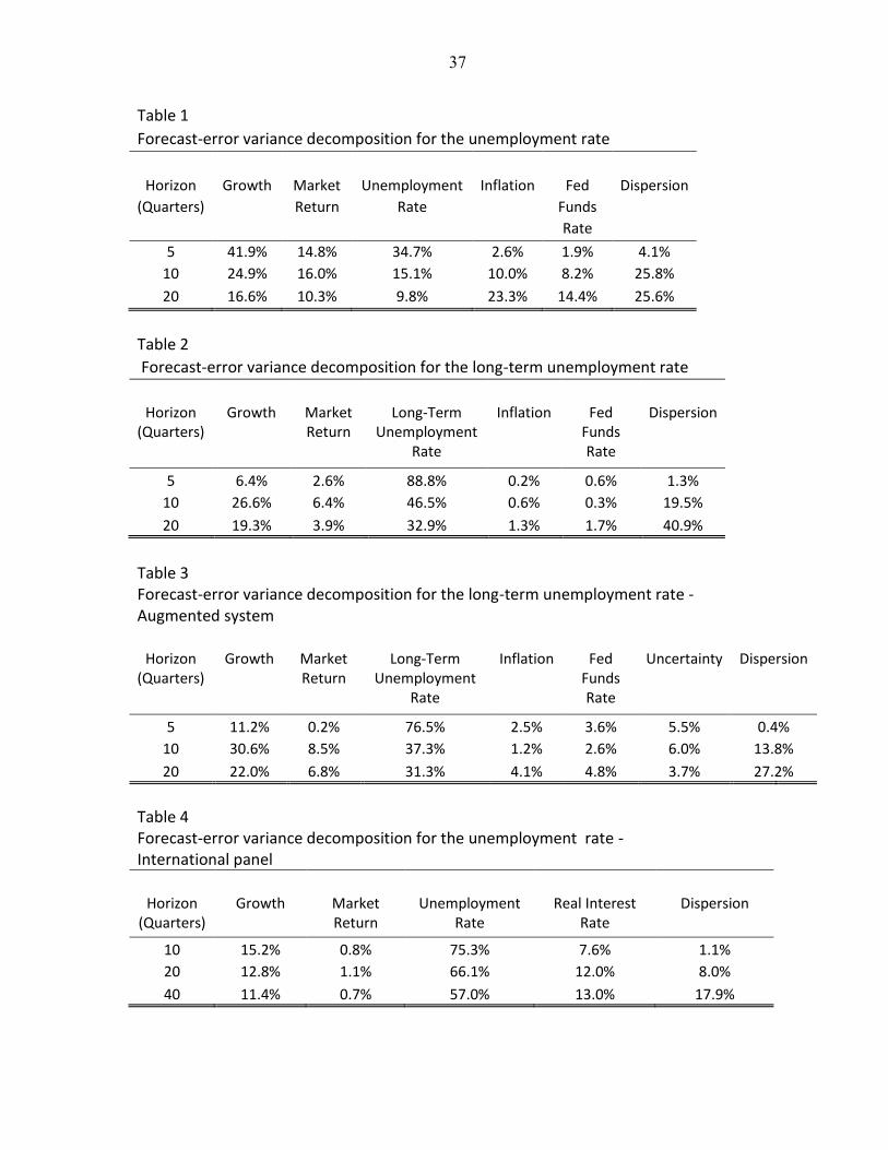
fluctuations. Tables 1 and 2 show the proportion of the forecast-error variance of overall

unemployment and long-term unemployment, respectively, that is explained by the various

shocks, given our identification scheme. At the 5-year horizon, about 25 percent of the

variance of unemployment forecast errors is explained by innovations to the dispersion

index. The proportion is much higher when we consider variations in long-term

unemployment. Looking once again at the 5-year horizon, innovations to the dispersion index

account for up to 40 percent of the overall variance, making it more important than any other

variable in the VAR, including the unemployment rate itself.

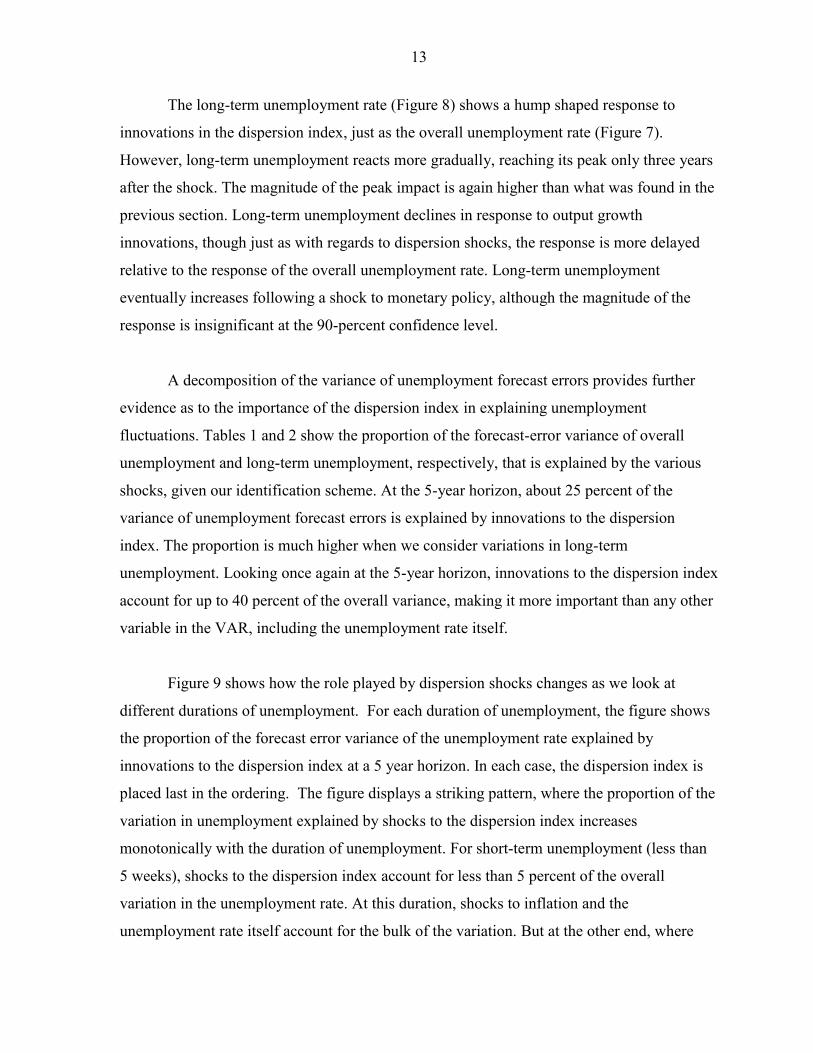
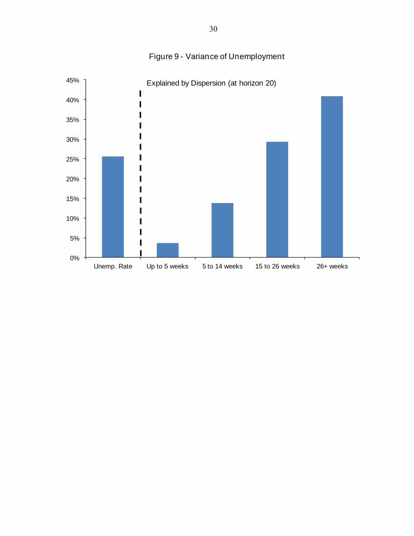
Figure 9 shows how the role played by dispersion shocks changes as we look at

different durations of unemployment. For each duration of unemployment, the figure shows

the proportion of the forecast error variance of the unemployment rate explained by

innovations to the dispersion index at a 5 year horizon. In each case, the dispersion index is

placed last in the ordering. The figure displays a striking pattern, where the proportion of the

variation in unemployment explained by shocks to the dispersion index increases

monotonically with the duration of unemployment. For short-term unemployment (less than

5 weeks), shocks to the dispersion index account for less than 5 percent of the overall

variation in the unemployment rate. At this duration, shocks to inflation and the

unemployment rate itself account for the bulk of the variation. But at the other end, where

14

duration exceeds 26 weeks, dispersion shocks account for about 40 percent of the variance of

the forecast error.

B. Sectoral Shocks and Long-Term Unemployment during the Great Recession

We now use the VAR estimated above to examine long-term unemployment during

the Great Recession. Long term unemployment (defined as those who were unemployed for

more than 26 weeks) constituted 16 percent of total unemployment in the fourth quarter of

2007 and 40 percent in the second quarter of 2010. Notably, it has remained high despite a

resumption of growth in output.

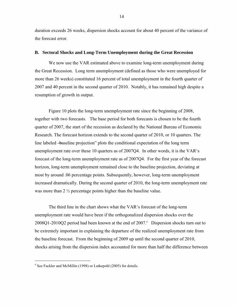
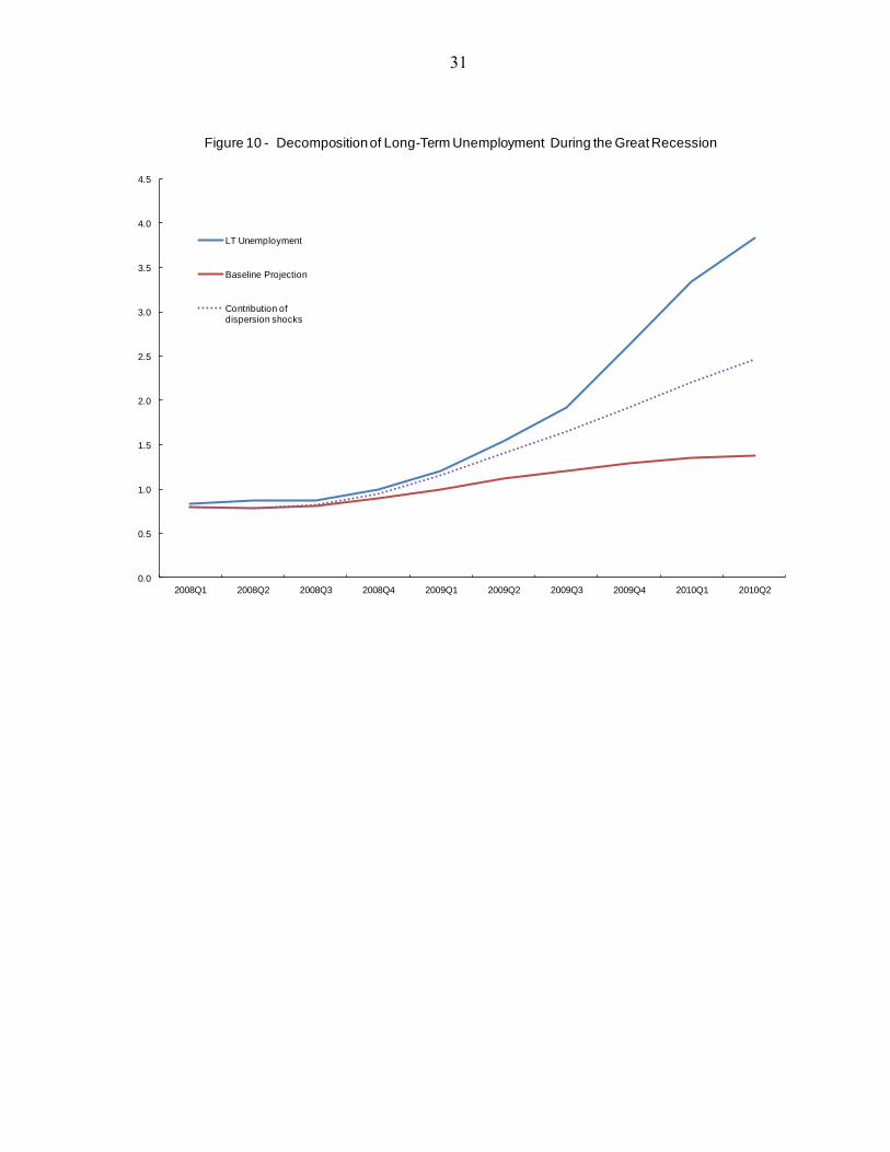
Figure 10 plots the long-term unemployment rate since the beginning of 2008,

together with two forecasts. The base period for both forecasts is chosen to be the fourth

quarter of 2007, the start of the recession as declared by the National Bureau of Economic

Research. The forecast horizon extends to the second quarter of 2010, or 10 quarters. The

line labeled ―baseline projection‖ plots the conditional expectation of the long term

unemployment rate over these 10 quarters as of 2007Q4. In other words, it is the VAR‘s

forecast of the long-term unemployment rate as of 2007Q4. For the first year of the forecast

horizon, long-term unemployment remained close to the baseline projection, deviating at

most by around .06 percentage points. Subsequently, however, long-term unemployment

increased dramatically. During the second quarter of 2010, the long-term unemployment rate

was more than 2 ½ percentage points higher than the baseline value.

The third line in the chart shows what the VAR‘s forecast of the long-term

unemployment rate would have been if the orthogonalized dispersion shocks over the

2008Q1-2010Q2 period had been known at the end of 2007.6 Dispersion shocks turn out to

be extremely important in explaining the departure of the realized unemployment rate from

the baseline forecast. From the beginning of 2009 up until the second quarter of 2010,

shocks arising from the dispersion index accounted for more than half the difference between

6 See Fackler and McMillin (1998) or Lutkepohl (2005) for details.

15

the actual long-term unemployment rate and its baseline projection. The contribution of

shocks to GDP growth, on the other hand, averaged about 15 percent during the same period.

C. Structural vs. Cyclical Movements in Unemployment

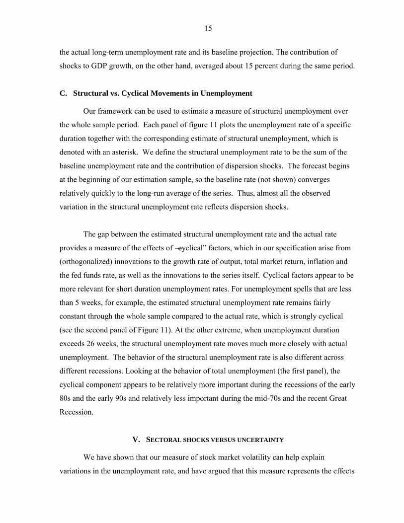
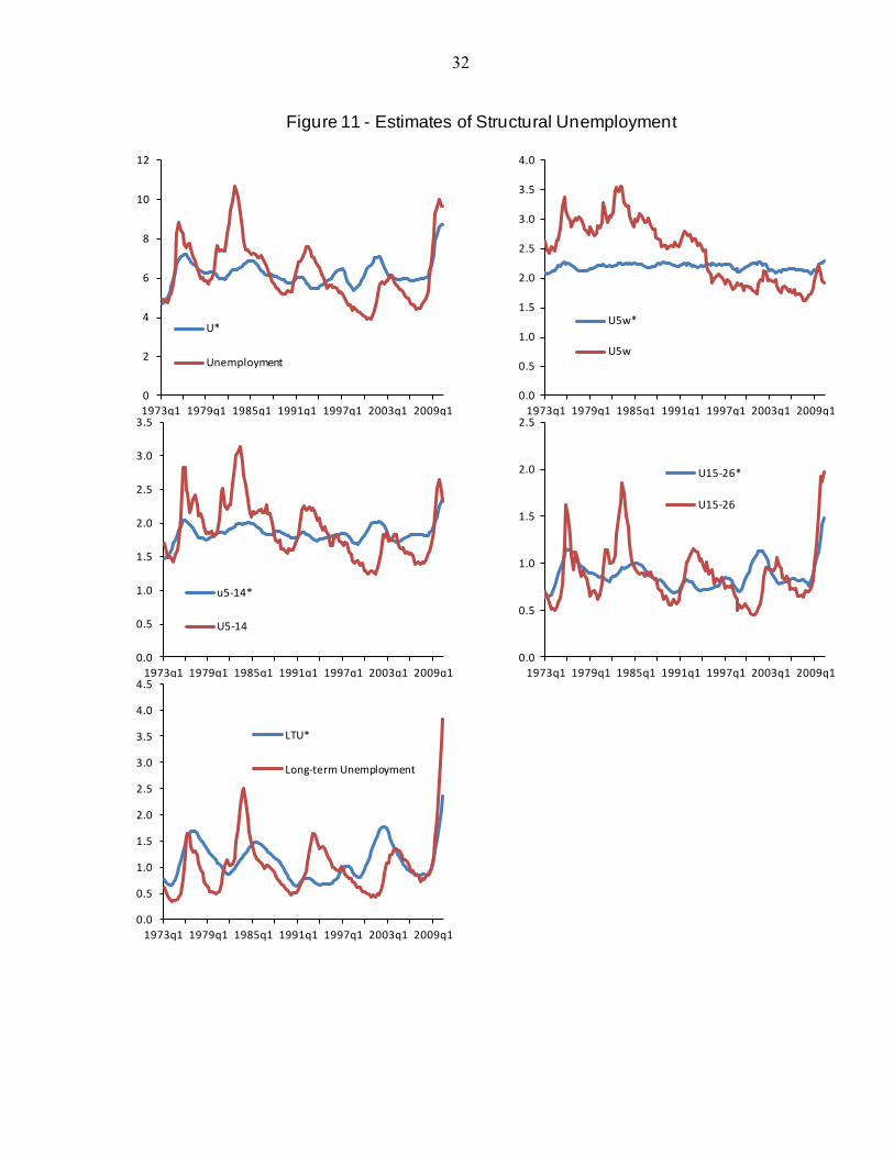
Our framework can be used to estimate a measure of structural unemployment over

the whole sample period. Each panel of figure 11 plots the unemployment rate of a specific

duration together with the corresponding estimate of structural unemployment, which is

denoted with an asterisk. We define the structural unemployment rate to be the sum of the

baseline unemployment rate and the contribution of dispersion shocks. The forecast begins

at the beginning of our estimation sample, so the baseline rate (not shown) converges

relatively quickly to the long-run average of the series. Thus, almost all the observed

variation in the structural unemployment rate reflects dispersion shocks.

The gap between the estimated structural unemployment rate and the actual rate

provides a measure of the effects of ―cyclical‖ factors, which in our specification arise from

(orthogonalized) innovations to the growth rate of output, total market return, inflation and

the fed funds rate, as well as the innovations to the series itself. Cyclical factors appear to be

more relevant for short duration unemployment rates. For unemployment spells that are less

than 5 weeks, for example, the estimated structural unemployment rate remains fairly

constant through the whole sample compared to the actual rate, which is strongly cyclical

(see the second panel of Figure 11). At the other extreme, when unemployment duration

exceeds 26 weeks, the structural unemployment rate moves much more closely with actual

unemployment. The behavior of the structural unemployment rate is also different across

different recessions. Looking at the behavior of total unemployment (the first panel), the

cyclical component appears to be relatively more important during the recessions of the early

80s and the early 90s and relatively less important during the mid-70s and the recent Great

Recession.

V. SECTORAL SHOCKS VERSUS UNCERTAINTY

We have shown that our measure of stock market volatility can help explain

variations in the unemployment rate, and have argued that this measure represents the effects

16

of sectoral shocks. But it is possible to place other interpretations on measures of stock

market volatility. In particular, Bloom (2009) has advocated the use of one such measure as

a proxy for uncertainty. He argues that an increase in uncertainty can have significant

negative effects on the economy, as firms optimally adopt a ―wait-and-see‖ approach to

capital expenditure and hiring decisions. As stressed by Bloom, these effects are temporary.

His VAR estimates show that an uncertainty shock causes employment to fall sharply over

the first 6 months, but the rebound is equally rapid. One year after the shock, employment is

higher than it was prior to the shock.

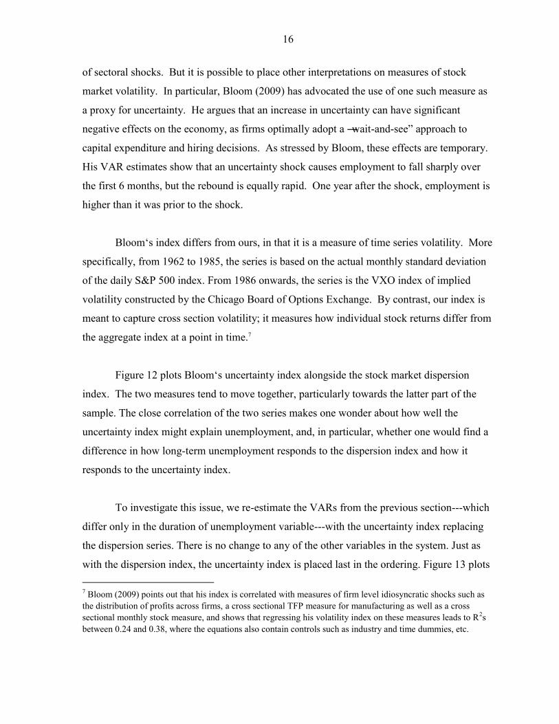
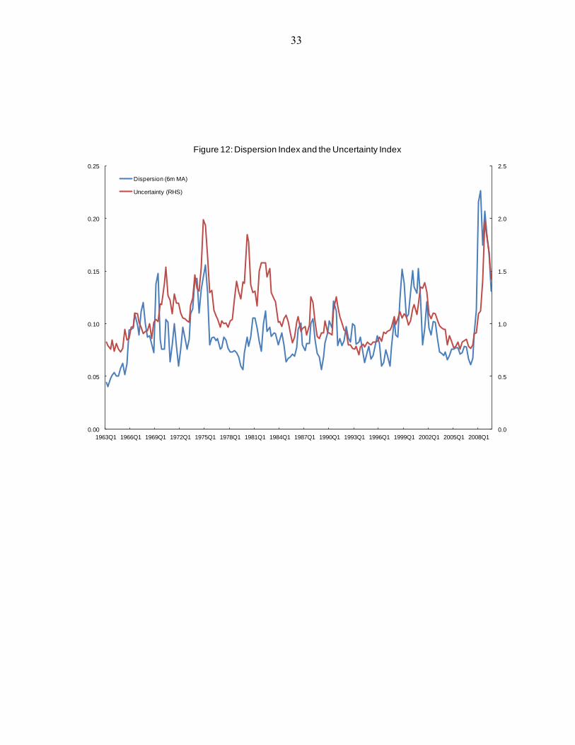
Bloom‘s index differs from ours, in that it is a measure of time series volatility. More

specifically, from 1962 to 1985, the series is based on the actual monthly standard deviation

of the daily S&P 500 index. From 1986 onwards, the series is the VXO index of implied

volatility constructed by the Chicago Board of Options Exchange. By contrast, our index is

meant to capture cross section volatility; it measures how individual stock returns differ from

the aggregate index at a point in time.7

Figure 12 plots Bloom‘s uncertainty index alongside the stock market dispersion

index. The two measures tend to move together, particularly towards the latter part of the

sample. The close correlation of the two series makes one wonder about how well the

uncertainty index might explain unemployment, and, in particular, whether one would find a

difference in how long-term unemployment responds to the dispersion index and how it

responds to the uncertainty index.

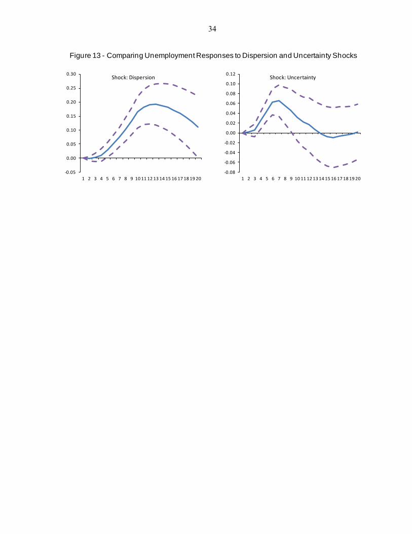
To investigate this issue, we re-estimate the VARs from the previous section---which

differ only in the duration of unemployment variable---with the uncertainty index replacing

the dispersion series. There is no change to any of the other variables in the system. Just as

with the dispersion index, the uncertainty index is placed last in the ordering. Figure 13 plots 7 Bloom (2009) points out that his index is correlated with measures of firm level idiosyncratic shocks such as the distribution of profits across firms, a cross sectional TFP measure for manufacturing as well as a cross sectional monthly stock measure, and shows that regressing his volatility index on these measures leads to R2s between 0.24 and 0.38, where the equations also contain controls such as industry and time dummies, etc.

17

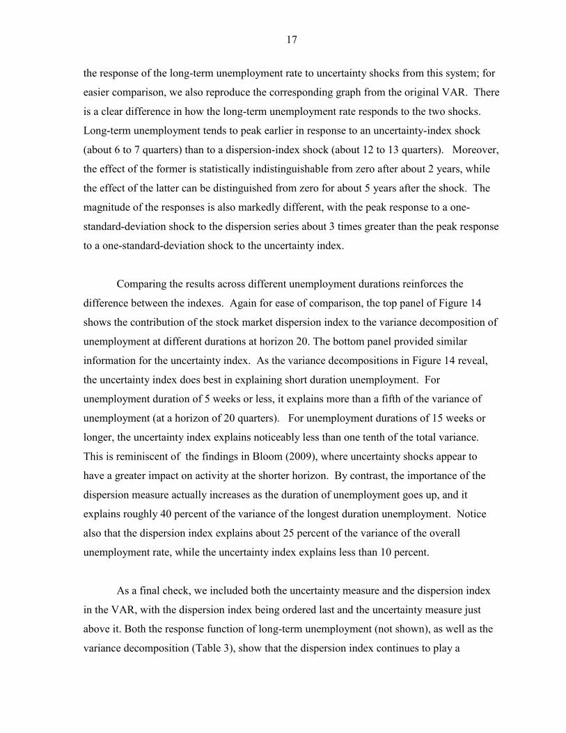
the response of the long-term unemployment rate to uncertainty shocks from this system; for

easier comparison, we also reproduce the corresponding graph from the original VAR. There

is a clear difference in how the long-term unemployment rate responds to the two shocks.

Long-term unemployment tends to peak earlier in response to an uncertainty-index shock

(about 6 to 7 quarters) than to a dispersion-index shock (about 12 to 13 quarters). Moreover,

the effect of the former is statistically indistinguishable from zero after about 2 years, while

the effect of the latter can be distinguished from zero for about 5 years after the shock. The

magnitude of the responses is also markedly different, with the peak response to a one-

standard-deviation shock to the dispersion series about 3 times greater than the peak response

to a one-standard-deviation shock to the uncertainty index.

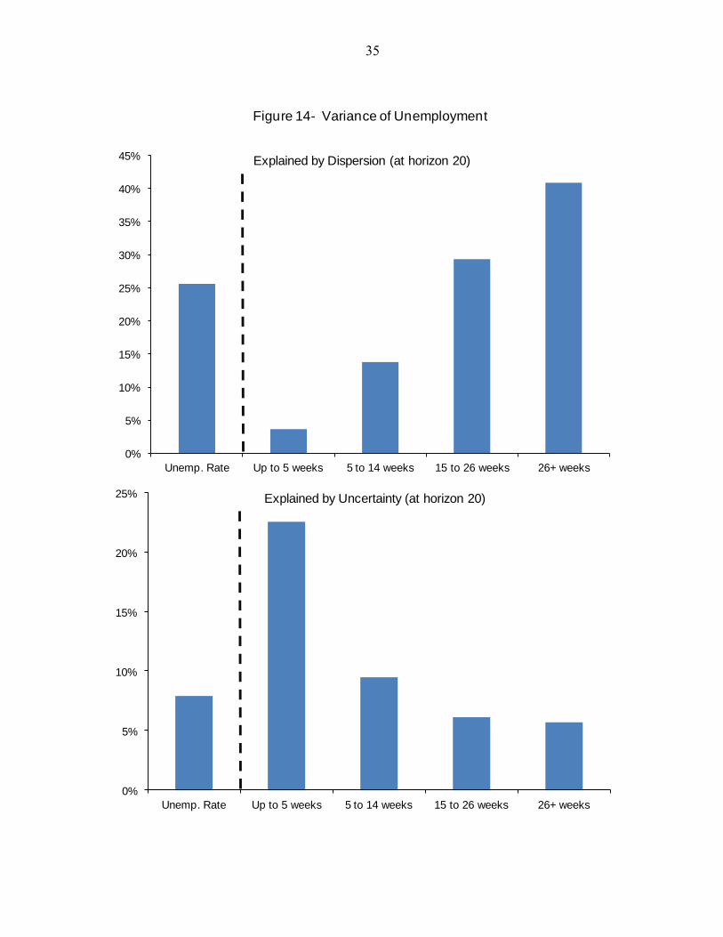
Comparing the results across different unemployment durations reinforces the

difference between the indexes. Again for ease of comparison, the top panel of Figure 14

shows the contribution of the stock market dispersion index to the variance decomposition of

unemployment at different durations at horizon 20. The bottom panel provided similar

information for the uncertainty index. As the variance decompositions in Figure 14 reveal,

the uncertainty index does best in explaining short duration unemployment. For

unemployment duration of 5 weeks or less, it explains more than a fifth of the variance of

unemployment (at a horizon of 20 quarters). For unemployment durations of 15 weeks or

longer, the uncertainty index explains noticeably less than one tenth of the total variance.

This is reminiscent of the findings in Bloom (2009), where uncertainty shocks appear to

have a greater impact on activity at the shorter horizon. By contrast, the importance of the

dispersion measure actually increases as the duration of unemployment goes up, and it

explains roughly 40 percent of the variance of the longest duration unemployment. Notice

also that the dispersion index explains about 25 percent of the variance of the overall

unemployment rate, while the uncertainty index explains less than 10 percent.

As a final check, we included both the uncertainty measure and the dispersion index

in the VAR, with the dispersion index being ordered last and the uncertainty measure just

above it. Both the response function of long-term unemployment (not shown), as well as the

variance decomposition (Table 3), show that the dispersion index continues to play a

18

significant role. For instance, at the 20 quarter horizon, the dispersion index explains about

27 percent of the forecast error variance of the long duration unemployment rate, while the

uncertainty index explains less than 4 percent.

VI. A VAR ESTIMATED ON INTERNATIONAL DATA

In this section, we present cross-country evidence on the importance of the stock

market dispersion index in explaining unemployment fluctuations. The suitability of this

index as a proxy for sectoral shocks will differ across countries depending on the depth of

their stock markets and whether or not the set of listed firms is representative of the whole

economy. The dispersion of stock market returns in relatively thin markets, for example,

could be very volatile due to the influence of a few large firms, or of foreign capital flows. In

order to minimize such distortions, we limit our analysis to a sample of advanced economies

that have relatively deep and broad stock markets. The countries in our sample are Australia,

Austria, Denmark, Finland, France, Germany, Italy, Netherlands, Norway, Portugal, Sweden,

and the United Kingdom.8

We did not add more countries to our sample because we were unable to get stock

market data of sufficient length. The move to an international setting forced us to confront

several other data issues as well. While data on stock returns at the industry level are

obtainable across countries, comparable disaggregate data on employment by industry are not

consistently available. A breakdown of sectoral employment at the broad national accounts

classification is available, but this is too coarse a breakdown to be applied to the more

disaggregated industry stock return data. As a result of this data limitation, we weight the

stock returns by the industry‘s share of market capitalization. To minimize large fluctuations

in these shares, we use a rolling 10-year average. A further data complication is the lack of

cross-country measures of monetary policy. Changes in nominal short-term interest rates,

unlike the fed funds rate, contain both policy-induced changes as well as other endogenous

responses to disturbances unrelated to policy shifts. Still, for this set of advanced economies,

8 Adding the U.S. to this sample does not make a material difference to the results below.

19

monetary policy is best represented by changes in interest rates. Therefore, instead of the

nominal rate, we combine the measures of inflation and the nominal interest rate to construct

an ex-post real interest rate, which we include in the VAR. Finally, long-term unemployment

rate data are not consistently available for these countries, i.e., we are unable to get data

series of sufficient length. Consequently, the analysis is limited to the overall unemployment

rate.

The setup of the VAR is similar to the previous section, but now the data have both a

cross-sectional and time-series dimension. As such, we estimate a panel VAR (see Love and

Zicchino, 2006, for example) where the coefficients on the VAR are restricted to be the same

across all cross-sectional units. Country-specific fixed effects, however, are included. The

ordering is the same as it was in the previous section: GDP growth is ordered first, followed

by total market return, unemployment, real interest rate and, lastly, the dispersion of stock

market returns. GMM methods are used to estimate the system is estimated over the period

1965:Q2 to 2008:Q3 (see Arellano and Bond, 1991, 1995).9 The lag length is set at 12

quarters.

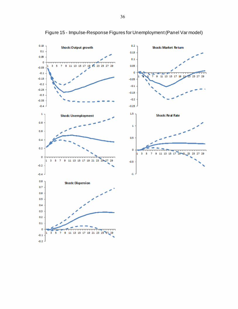
The impulse-response functions for unemployment are shown in Figure 15. Each

panel shows the response of the unemployment rate to a one-standard-deviation shock, with

the residuals orthogonalized according to the ordering above. The impulse-response graphs

look similar to those for the U.S. For instance, unemployment increases after an increase in

stock market dispersion and decreases after a positive growth shock. Interestingly, the

magnitude of the responses is also of the same order. A one-standard-deviation shock to the

dispersion index results in a maximum increase of about 0.3 percentage points in the

unemployment rate here, just as it did for U.S. data. However, the response of unemployment

to the dispersion shock is noticeably delayed; it also persists for much longer. In the cross-

country data, the peak impact on unemployment is reached only after 6 years, while the peak

in U.S. data is reached after 2 years.

9 For most countries, however, the stock market data only starts in 1973.

20

The other impulse responses also show more persistence in the international panel

than they do for the U.S. data. For instance, the response of the unemployment rate to an

unemployment rate shock is statistically indistinguishable from zero less than two years after

the shock in the U.S. data set (Figure 7), but can still be distinguished from zero more than

six years after the shock in the international data set (Figure 15). Many observers have

noted the tendency of the unemployment rates in European countries10 to stay high for long

periods of time following adverse shocks. This has led to discussions of hysteresis in the

unemployment rate; see Blanchard and Summers (1986) for an early example, or Blanchard

(2006) for a more recent discussion.

The dispersion index also continues to account for a significant proportion of the

forecast error variance for unemployment, and—as in the U.S. data—its importance grows

over time. Table 4 shows that at a forecast horizon of 40 quarters, dispersion shocks account

for about 18 percent of the variation in the unemployment rate. This is about three-fourths of

what we get for the U.S. data at the same horizon. And just as in the U.S. data, apart from

shocks to the unemployment rate itself, dispersion shocks are the most important in

explaining the variance of the unemployment rate at long horizons.

VII. CONCLUSION

We have shown that structural shocks (as measured by an index of the cross section

variance of stock prices) have a substantial impact on the unemployment rate in a sample that

includes the Great Recession of 2007-2009. Further, these shocks become more important as

the duration of unemployment increases, a finding that accords with the intuition that such

shocks should be associated with longer spells of search, as they cause workers to move

across sectors.

An examination of the Great Recession shows that sectoral shocks account for about

half of the increase in the long duration unemployment rate that has taken place over this

period. Once again, this accords with informal evidence about employment conditions in the 10 With the exception of Australia, all the countries in our sample are in Europe.

21

construction sector and, to a lesser extent, in finance. In this, the Great Recession is similar

to the recession of 1973-75, as sectoral shocks appear to have played a large role at that time

as well.

We have also shown that our measure of cross section volatility is quite different

from the measure of time series volatility proposed by Bloom (2009). In particular, Bloom‘s

measure does very well at explaining short duration unemployment, but has a small impact

on long duration unemployment. By contrast, our measure does better the longer the

duration of unemployment under consideration. We interpret these findings to mean that

both measures are well suited to the purpose for which they were designed. The time series

measure is meant to capture uncertainty, and Bloom emphasizes that uncertainty has a short

run effect. By contrast, our measure is meant to capture shocks that cause reallocation across

sectors, and such reallocation is going to take time.

Finally, we have shown that the dispersion index continues to matter in a sample of a

dozen advanced economies. While we have not been able to find adequate data on long

duration unemployment for these countries, we have shown that an increase in stock market

dispersion leads to a substantial and significant increase in the unemployment rate, even after

we control for output, inflation and the value of the stock market.

22

5

10

15

20

25

30

35

40

1963Q1 1966Q1 1969Q1 1972Q1 1975Q1 1978Q1 1981Q1 1984Q1 1987Q1 1990Q1 1993Q1 1996Q1 1999Q1 2002Q1 2005Q1 2008Q1 2011Q1

Figure 1 - Average Duration of Unemployment (Weeks)

23

Figure 2 - Duration of Unemployment (percent of labor force)

0.0

0.5

1.0

1.5

2.0

2.5

3.0

3.5

4.0

1963Q1 1972Q1 1981Q1 1990Q1 1999Q1 2008Q1

Less than 5 weeks

0.0

0.5

1.0

1.5

2.0

2.5

3.0

3.5

1963Q1 1972Q1 1981Q1 1990Q1 1999Q1 2008Q1

5 to 14 weeks

0.0

0.5

1.0

1.5

2.0

2.5

1963Q1 1972Q1 1981Q1 1990Q1 1999Q1 2008Q1

15 to 26 weeks

0.0

1.0

2.0

3.0

4.0

5.0

1963Q1 1972Q1 1981Q1 1990Q1 1999Q1 2008Q1

27 weeks and over

24

-2.0

-1.0

0.0

1.0

2.0

3.0

4.0

5.0

Figure 3 - Change in Unemployment Rate 2007-09 (Percent)

25

0.00

0.05

0.10

0.15

0.20

0.25

1963Q1 1968Q1 1973Q1 1978Q1 1983Q1 1988Q1 1993Q1 1998Q1 2003Q1 2008Q1

Figure 4 - Stock Market Returns Dispersion Index (6-month moving average)

26

Figure 5 - Impulse-Response Figures for Unemployment (Univariate model)

-0.2

0.0

0.2

0.4

0.6

0.8

1.0

1.2

1 2 3 4 5 6 7 8

Impact of MP shock

-0.1

-0.1

0.0

0.1

0.1

0.2

0.2

0.3

1 2 3 4 5 6 7 8

Impact of FP shock

-0.1

0.0

0.1

0.2

0.3

0.4

0.5

1 2 3 4 5 6 7 8

Impact of oil price increase

0.0

0.1

0.1

0.2

0.2

0.3

0.3

1 2 3 4 5 6 7 8

Impact of increase in dspersion index

27

Figure 6 - Impulse-Response Figures for Long-Term Unemployment (Univariate model)

-0.25

-0.20

-0.15

-0.10

-0.05

0.00

0.05

1 2 3 4 5 6 7 8

Impact of MP shock on LTU

-0.08

-0.06

-0.04

-0.02

0.00

0.02

0.04

1 2 3 4 5 6 7 8

Impact of FP shock on LTU

-0.08

-0.07

-0.06

-0.05

-0.04

-0.03

-0.02

-0.01

0.00

0.01

0.02

1 2 3 4 5 6 7 8

Impact of oil price increase on LTU

-0.04

-0.02

0.00

0.02

0.04

0.06

0.08

0.10

0.12

0.14

1 2 3 4 5 6 7 8

Impact of increase in dspersion index on LTU

28

Figure 7 - Impulse-Response Figures for Unemployment (VAR model)

-0.5

-0.4

-0.3

-0.2

-0.1

0.0

0.1

0.2

0.3

0.4

1 2 3 4 5 6 7 8 9 10 11 12 13 14 15 16 17 18 19 20

Shock: Output Growth

-0.4

-0.3

-0.2

-0.1

0.0

0.1

0.2

0.3

1 2 3 4 5 6 7 8 9 10 11 12 13 14 15 16 17 18 19 20

Shock: Market Return

-0.2

-0.1

-0.1

0.0

0.1

0.1

0.2

0.2

0.3

0.3

0.4

1 2 3 4 5 6 7 8 9 10 11 12 13 14 15 16 17 18 19 20

Shock: Unemployment

-0.05

0.00

0.05

0.10

0.15

0.20

0.25

0.30

0.35

0.40

0.45

1 2 3 4 5 6 7 8 9 10 11 12 13 14 15 16 17 18 19 20

Shock: Inflation

-0.2

-0.1

0.0

0.1

0.2

0.3

0.4

0.5

1 2 3 4 5 6 7 8 9 10 11 12 13 14 15 16 17 18 19 20

Shock: Fed Funds Rate

-0.2

-0.1

0.0

0.1

0.2

0.3

0.4

0.5

1 2 3 4 5 6 7 8 9 10 11 12 13 14 15 16 17 18 19 20

Shock: Dispersion

29

Figure 8 - Impulse-Response Figures for Long-Term Unemployment (VAR model)

-0.25

-0.20

-0.15

-0.10

-0.05

0.00

0.05

0.10

1 2 3 4 5 6 7 8 9 10 11 12 13 14 15 16 17 18 19 20

Shock: Output Growth

-0.20

-0.15

-0.10

-0.05

0.00

0.05

0.10

1 2 3 4 5 6 7 8 9 10 11 12 13 14 15 16 17 18 19 20

Shock: Market Return

-0.10

-0.05

0.00

0.05

0.10

0.15

0.20

0.25

1 2 3 4 5 6 7 8 9 10 11 12 13 14 15 16 17 18 19 20

Shock: LT Unemployment

-0.10

-0.05

0.00

0.05

0.10

0.15

1 2 3 4 5 6 7 8 9 10 11 12 13 14 15 16 17 18 19 20

Shock: Inflation

-0.08

-0.06

-0.04

-0.02

0.00

0.02

0.04

0.06

0.08

0.10

0.12

0.14

1 2 3 4 5 6 7 8 9 10 11 12 13 14 15 16 17 18 19 20

Shock: Fed Funds Rate

-0.05

0.00

0.05

0.10

0.15

0.20

0.25

0.30

1 2 3 4 5 6 7 8 9 10 11 12 13 14 15 16 17 18 19 20

Shock: Dispersion

30

Figure 9 - Variance of Unemployment

0%

5%

10%

15%

20%

25%

30%

35%

40%

45%

Unemp. Rate Up to 5 weeks 5 to 14 weeks 15 to 26 weeks 26+ weeks

Explained by Dispersion (at horizon 20)

31

0.0

0.5

1.0

1.5

2.0

2.5

3.0

3.5

4.0

4.5

2008Q1 2008Q2 2008Q3 2008Q4 2009Q1 2009Q2 2009Q3 2009Q4 2010Q1 2010Q2

Figure 10 - Decomposition of Long-Term Unemployment During the Great Recession

LT Unemployment

Baseline Projection

Contribution of dispersion shocks

32

Figure 11 - Estimates of Structural Unemployment

0

2

4

6

8

10

12

1973q1 1979q1 1985q1 1991q1 1997q1 2003q1 2009q1

U*

Unemployment

0.0

0.5

1.0

1.5

2.0

2.5

3.0

3.5

4.0

1973q1 1979q1 1985q1 1991q1 1997q1 2003q1 2009q1

U5w*

U5w

0.0

0.5

1.0

1.5

2.0

2.5

3.0

3.5

1973q1 1979q1 1985q1 1991q1 1997q1 2003q1 2009q1

u5-14*

U5-14

0.0

0.5

1.0

1.5

2.0

2.5

1973q1 1979q1 1985q1 1991q1 1997q1 2003q1 2009q1

U15-26*

U15-26

0.0

0.5

1.0

1.5

2.0

2.5

3.0

3.5

4.0

4.5

1973q1 1979q1 1985q1 1991q1 1997q1 2003q1 2009q1

LTU*

Long-term Unemployment

33

0.0

0.5

1.0

1.5

2.0

2.5

0.00

0.05

0.10

0.15

0.20

0.25

1963Q1 1966Q1 1969Q1 1972Q1 1975Q1 1978Q1 1981Q1 1984Q1 1987Q1 1990Q1 1993Q1 1996Q1 1999Q1 2002Q1 2005Q1 2008Q1

Figure 12: Dispersion Index and the Uncertainty Index

Dispersion (6m MA)

Uncertainty (RHS)

34

Figure 13 - Comparing Unemployment Responses to Dispersion and Uncertainty Shocks

-0.05

0.00

0.05

0.10

0.15

0.20

0.25

0.30

1 2 3 4 5 6 7 8 9 10 11 12 13 14 15 16 17 18 19 20

Shock: Dispersion

-0.08

-0.06

-0.04

-0.02

0.00

0.02

0.04

0.06

0.08

0.10

0.12

1 2 3 4 5 6 7 8 9 10 11 12 13 14 15 16 17 18 19 20

Shock: Uncertainty

35

Figure 14- Variance of Unemployment

0%

5%

10%

15%

20%

25%

30%

35%

40%

45%

Unemp. Rate Up to 5 weeks 5 to 14 weeks 15 to 26 weeks 26+ weeks

Explained by Dispersion (at horizon 20)

0%

5%

10%

15%

20%

25%

Unemp. Rate Up to 5 weeks 5 to 14 weeks 15 to 26 weeks 26+ weeks

Explained by Uncertainty (at horizon 20)

36

Figure 15 - Impulse-Response Figures for Unemployment (Panel Var model)

37

Table 1

Forecast-error variance decomposition for the unemployment rate

Horizon

(Quarters)

Growth Market

Return

Unemployment

Rate

Inflation Fed

Funds

Rate

Dispersion

5 41.9% 14.8% 34.7% 2.6% 1.9% 4.1%

10 24.9% 16.0% 15.1% 10.0% 8.2% 25.8%

20 16.6% 10.3% 9.8% 23.3% 14.4% 25.6%

Table 2

Forecast-error variance decomposition for the long-term unemployment rate

Horizon

(Quarters) Growth Market

Return Long-Term

Unemployment Rate

Inflation Fed Funds Rate

Dispersion

5 6.4% 2.6% 88.8% 0.2% 0.6% 1.3%

10 26.6% 6.4% 46.5% 0.6% 0.3% 19.5%

20 19.3% 3.9% 32.9% 1.3% 1.7% 40.9%

Table 3 Forecast-error variance decomposition for the long-term unemployment rate - Augmented system

Horizon

(Quarters) Growth Market

Return Long-Term

Unemployment Rate

Inflation Fed Funds Rate

Uncertainty Dispersion

5 11.2% 0.2% 76.5% 2.5% 3.6% 5.5% 0.4%

10 30.6% 8.5% 37.3% 1.2% 2.6% 6.0% 13.8%

20 22.0% 6.8% 31.3% 4.1% 4.8% 3.7% 27.2%

Table 4 Forecast-error variance decomposition for the unemployment rate - International panel

Horizon

(Quarters) Growth Market

Return Unemployment

Rate Real Interest

Rate Dispersion

10 15.2% 0.8% 75.3% 7.6% 1.1%

20 12.8% 1.1% 66.1% 12.0% 8.0%

40 11.4% 0.7% 57.0% 13.0% 17.9%

38

REFERENCES

Abraham, Katharine, and Lawrence Katz. 1986. ―Cyclical Unemployment: Sectoral Shifts or Aggregate Disturbances?‖ Journal of Political Economy 94, pp. 507–522.

Aaronson, Daniel, Rissman, Ellen R., and Sullivan, Daniel G., 2004, ―Can Sectoral Reallocation Explain the Jobless Recovery?‖ Economic Perspectives, Federal Reserve Bank of Chicago.

Cerra, Valerie, and Sweta Chaman Saxena, 2008, ―Growth Dynamics: The Myth of Economic Recovery,‖ American Economic Review, Vol. 98(1), pp. 439-57. Ball, Laurence, 1999 ―Aggregate Demand and Long-Run Unemployment.‖ Brookings Papers on Economic Activity, 1999.

Barnichon, Regis, Figura, Andrew, 2010. ―What Drives Matching Efficiency? A tale of Composition and Dispersion.‖ Finance and Economics Discussion Series, Federal Reserve Board, 2011-10.

Barnichon, Regis, Elsby, Michael, Hobijn, Bart, and Aysegul, Sahin, 2010. ―Which Industries are Changing the Beveridge Curve?‖ Federal Reserve Bank of San Francisco, Working Paper 2010-32.

Barro, Robert J. 1986. ―Comment on ‗Do Equilibrium Real Business Theories Explain Postwar U.S. Business Cycles?‘‖ NBER Macroeconomics Annual 1, pp. 135–139.

Beaudry, Paul, and Portier, Franck, 2004. ―Stock Prices, News and Economic Fluctuations.‖ NBER Working Paper No. 10548.

Benjamin, Daniel and Levis Kochin, 1979. ―Searching for an Explanation of Unemployment in Interwar Britain,‖ Journal of Political Economy, vol. 87, no. 3.

Bernanke, Ben, and Alan Blinder. 1992. ―The Federal Funds Rate and the Channels of Monetary Transmission.‖ American Economic Review (September) pp. 901–921.

Black, Fisher. 1995. Exploring General Equilibrium. Cambridge: MIT Press.

__________. 1987. Business Cycles and Equilibrium. New York: Basil Blackwell.

Blanchard, Olivier. 2006. ―European Unemployment: The Evolution of Facts and Ideas,‖ Economic Policy, 45(1), pp. 5-59.

__________ and Lawrence Summers. 1986. ―Hysteresis and the European Unemployment Problem,‖ NBER Macroeconomics Annual 1, Cambridge:MIT Press, pp. 15-78.

39

Bloom, Nicholas, 2009. ―The Impact of Uncertainty Shocks‖ Econometrica (May), pp. 623-85.

Bloom, Nicholas, Max Floetotto and Nir Jaimovich, 2010, ―Really Uncertain Business Cycles,‖ Stanford University, working paper.

Brainard, Lael, 1992. ―Sectoral Shifts and Unemployment in Interwar Britain,‖ NBER Working Paper No. W3980. Brainard, Lael, and David Cutler. 1993. ―Sectoral Shifts and Cyclical Unemployment.‖

Quarterly Journal of Economics, pp. 219–243. Campbell, Jeffrey, and Kenneth Kuttner. 1996. ―Macroeconomic Effects of Employment Reallocation.‖ Carnegie-Rochester Conference Series on Public Policy (June) pp. 87–117. Christiano, Lawrence J., Martin Eichenbaum and Charles L. Evans, 1999. ―Monetary Policy Shocks: What Have We Learned and To What End?‖ In J.B. Taylor and M. Woodford, eds., Handbook of Macroeconomics, Vol. 1. Amsterdam: Elsevier B.V. Clague, Ewan, 1935. ―The Problem of Unemployment and the Changing Structure of Industry,‖ Journal of the American Statistical Association, vol. 30, no. 189, Supplement, pp. 209-14. Cochrane, John H. 1994. ―Shocks.‖ NBER Working Paper No. 4698.

Daly, Mary, Hobijn, Bart, and Valleta, Rob, 2011. ―The Recent Evolution of the Natural Rate of Unemployment.‖ Federal Reserve Bank of San Francisco, Working Paper 2011-05.

Davis, Steve. 1987. ―Fluctuations in the Pace of Labor Reallocation.‖ Carnegie - Rochester Conference Series on Public Policy 27 (Spring) pp. 335–402.

__________. 1985. ―Allocative Disturbances and Temporal Asymmetry in Labor Market Fluctuations.‖ Working Paper. University of Chicago Graduate School of Business.

Elsby, Michael, Hobijn, Bart, and Aysegul, Sahin, 2010. ―The Labor Market in the Great Recession.‖ Brookings Panel on Economic Activity, March, 2010.

Estevao, Marcello and Evridiki Tsounta, 2011, ―Has the Great Recession Raised U.S. Structural Unemployment?‖, forthcoming IMF Working Paper.

40

Fackler, James and W. Douglas McMillin. 1998. "Historical Decomposition of Aggregate Demand and Supply Shocks in a Small Macro Model." Southern Economic Journal 64: 648-664.

Fortin, Mario, and Araar, Abdelkrim. 1997. ―Sectoral Shifts, Stock Market Dispersion and Unemployment in Canada.‖ Applied Economics, Vol. 29, Issue 6, 1997, pp. 829-839.

Gallipoli, Giovanni and Gianluigi Pelloni. 2008. ―Aggregate Shocks vs. Reallocation Shocks: An Appraisal of the Literature.‖ Rimini Center of Economic Analysis, Working Paper No. 27-08.

Groshen, Erica and Simon Potter, 2003, ―Has Structural Change Contributed to a Jobless Recovery?‖ Federal Reserve Bank of New York, Current Issues in Economics and Finance, Vol. 9, Number 8 Hall, Robert E. 1995. ―Lost Jobs.‖ Brookings Papers on Economic Activity No. 1, pp. 221–256.

__________. 1993. ―Macro Theory and the Recession of 1990–1991.‖ American Economic

Review Papers and Proceedings , pp. 275–279. Haltiwanger, John, 2010. ―The Changing Cyclical Dynamics of U.S. Labor Markets.‖

IMF, 2010, Unemployment Dynamics During Recessions and Recoveries: Okun's Law and Beyond (R. Balakrishnan, M. Das and P. Kannan), Chapter 3, World Economic Outlook, Spring 2010.

Kirkegaard, Jacob Funk, 2009, ―Structural and Cyclical Trends in Net Employment over U.S. Business Cycles, 1949-2009: Implications for the Next Recovery and Beyond,‖ Peterson Institute for International Economics, WP 09-5.

Kocherlakota, 2010, ―Inside the FOMC,‖ Speech at Marquette, Michigan, August 17. Krugman, 2010, ―Debunking the Structural Unemployment Myth,‖ New York Times, September 28.

Levine, Linda, 2009, ―The Labor Market during the Great Depression and the Current Recession.‖ Congressional Research Service, June, 2009.

Lilien, David. 1982. ―Sectoral Shifts and Cyclical Unemployment.‖ Journal of Political Economy 90, pp. 777–793.

Loungani, Prakash. 1986. ―Oil Price Shocks and the Dispersion Hypothesis.‖ Review of Economics and Statistics (August) pp. 536–539.

41

__________, Mark Rush, and William Tave. 1990. ―Stock Market Dispersion and

Unemployment.‖ Journal of Monetary Economics (June) pp. 367–388. __________ and Bharat Trehan. 1997. ―Explaining Unemployment: Sectoral vs. Aggregate

Shocks.‖ Federal Reserve Bank of San Francisco Economic Review, pp. 3-15. __________, Richard Rogerson, and Yang Hoon Sonn. 1989. ―Unemployment and Sectoral

Shifts: Evidence from PSID Data.‖ Working Paper. University of Florida. Lu, Jing, ―Aggregate Disturbances or Sectoral Shifts: Canadian Evidence.‖ The Canadian Journal of Economics, Vol. 30.

Love, Inessa, Zicchino, Lea, 2006. Financial Development and Dynamic Investment Behavior: Evidence from Panel VAR. The Quarterly Review of Economics and Finance, Vol. 46(2), pp 190-210.

Lutkepohl, H. 2005. ―New Introduction to Multiple Time Series Analysis.‖, Springer-Verlag, Berlin.

Mishel, Lawrence, Shierholz, and Edwards Kathryn, 2010. ―Reasons for Skepticism about Structural Employment‖ Economic Policy Institute, Briefing Paper no. 279.

Nason, James and Shaun Vahey, 2006, ―Interwar U.K. unemployment: the Benjamin and Kochin hypothesis or the legacy of ―just‖ taxes?‖, Federal Reserve Bank of Atlanta, Working Paper 2006-04.

Perry, George, and Charles Schultze. 1993. ―Was This Recession Different? Are They All Different?‖ Brookings Papers on Economic Activity 1, pp. 145–195.

Phelan, Christopher & Trejos, Alberto, 2000. "The aggregate effects of sectoral reallocations," Journal of Monetary Economics, vol. 45(2), pp. 249-68, April.

Polivka, Anne E., and Stephen M. Miller. 1995. ―The CPS after the Redesign: Refocusing the Economic Lens.‖ Mimeo. Bureau of Labor Statistics.

Rissman, Ellen R., 2009. ―Employment Growth: Cyclical Movements or Structural Change?‖ Economic Perspectives.

Romer, Christina, and David Romer. 1989. ―Does Monetary Policy Matter: A New Test in the Spirit of Friedman and Schwartz,‖ NBER Macroeconomics Annual, pp. 121–170.

Romer, Christina D., and David H. Romer. 2004. ―A New Measure of Monetary Shocks: Derivation and Implications.‖ American Economic Review 94, pp 1055-1084.

42

Romer, Christina D., and David H. Romer. 2010. ―A Narrative Analysis of Postwar Tax Changes.‖

Sahin, Aysegul, Joseph Song, Giorgio Topa and Gianluca Violante, ―Mismatch in the Labor Market: Evidence from the U.S. and the U.K., 2011.

Shin, Kwanho, 1997 ― Inter- and Intrasectoral Shocks: Effects on the Unemployment Rate.‖ Journal of Labor Economics, 1997, vol. 15, no 2.

Thomas, Jonathan. 1996. ―An Empirical Model of Sectoral Movements by Unemployed Workers,‖ Journal of Labor Economics (January) pp. 126–153.

Toledo, Wilfredo, and Milton Marquis. 1993. ―Capital Allocative Disturbances and Economic Fluctuations.‖ Review of Economics and Statistics (May) pp. 233–240.

Valletta, Robert G. 1996. ―Has Job Security in the U.S. Declined?‖ Federal Reserve Bank of San Francisco Economic Letter 96-06 (February 16).