NBER WORKING PAPER SERIES

NEW EVIDENCE ON THE IMPACT OF FINANCIAL CRISES IN ADVANCEDCOUNTRIES

Christina D. RomerDavid H. Romer

Working Paper 21021http://www.nber.org/papers/w21021

NATIONAL BUREAU OF ECONOMIC RESEARCH1050 Massachusetts Avenue

Cambridge, MA 02138March 2015

We are grateful to Steven Braun, Jesus Fernandez-Villaverde, Jason Furman, Mark Gertler, Pierre-OlivierGourinchas, Luc Laeven, Daniel Leigh, Demian Pouzo, James Powell, Carmen Reinhart, KennethRogoff, and seminar participants at Harvard University, the University of California, Berkeley, theUniversity of Chicago, the Banque de France, and the National Bureau of Economic Research forhelpful comments and discussions; to Marc Dordal i Carreras, Dmitri Koustas, and Walker Ray forresearch assistance; and to the Center for Equitable Growth at the University of California, Berkeleyfor financial support. The views expressed herein are those of the authors and do not necessarily reflectthe views of the National Bureau of Economic Research.

NBER working papers are circulated for discussion and comment purposes. They have not been peer-reviewed or been subject to the review by the NBER Board of Directors that accompanies officialNBER publications.

© 2015 by Christina D. Romer and David H. Romer. All rights reserved. Short sections of text, notto exceed two paragraphs, may be quoted without explicit permission provided that full credit, including© notice, is given to the source.

New Evidence on the Impact of Financial Crises in Advanced CountriesChristina D. Romer and David H. RomerNBER Working Paper No. 21021March 2015JEL No. E32,E44,G01,N10,N20

ABSTRACT

This paper examines the aftermath of financial crises in advanced countries in the four decades beforethe Great Recession. We construct a new series on financial distress in 24 OECD countries for theperiod 1967–2007. The series is based on assessments of the health of countries’ financial systemsfrom a consistent, real-time narrative source; and it classifies financial distress on a relatively finescale, rather than treating it as a 0-1 variable. We find that output declines following financial crisesin modern advanced countries are highly variable, on average only moderate, and often temporary.One important driver of the variation in outcomes across crises appears to be the severity and persistenceof the financial distress itself.

Christina D. RomerDepartment of EconomicsUniversity of California, BerkeleyBerkeley, CA 94720-3880and NBERcromer@econ.berkeley.edu

David H. RomerDepartment of EconomicsUniversity of California, BerkeleyBerkeley, CA 94720-3880and NBERdromer@econ.berkeley.edu

I. INTRODUCTION

The question of what happens to economies after a financial crisis is important to

identifying the sources of macroeconomic fluctuations, understanding interactions between the

financial sector and the real economy, and addressing a wide range of policy issues. In recent

years, a new conventional wisdom has emerged about the answer to this question: the

aftermath of financial crises is typically severe and long-lasting.1

Issues. Several aspects of previous research suggest that widespread acceptance of this

view may be premature, at least in the case of modern, advanced economies. A first issue is that

much of the evidence of severe effects of financial crises comes from the pre-World War II

period and from emerging economies. Differences in institutions, policy responses, and

industrial composition may make the experiences of prewar and emerging economies

unrepresentative of the impact of crises in modern advanced countries. But relatively little work

has focused specifically on the aftermath of crises in such economies.

A second issue involves the identification of financial crises. A key input to any study of the

impact of crises is a chronology of when they occurred, and a number of such chronologies exist.

But there are reasons to be concerned about them. Most obviously, the existing chronologies

sometimes differ substantially from one another. For example, both Reinhart and Rogoff

(2009a) and the International Monetary Fund (IMF) Systemic Banking Crises Database (Laeven

and Valencia, 2014) identify a crisis in Norway following the collapse of house prices in the late

1980s; but Reinhart and Rogoff date it as occurring from 1987 to 1993, while the IMF dates it as

running from the second half of 1991 to 1993. More generally, the specification of what

constitutes a crisis is often imprecise. To the degree that it is made concrete, it often combines a

range of distinct phenomena, such as asset price declines, banking problems, and consumer or

business bankruptcies. This absence of precise criteria can produce inconsistencies in the

1 We discuss recent scholarly work on the aftermath of financial crises below. For a popular example describing this as the conventional wisdom, see http://www.huffingtonpost.com/2012/11/01/bill-clinton-economist-kenneth-rogoff-obama_n_2061734.html.

2

identification of crises. Further, the interaction of the somewhat vague criteria for what

constitutes a crisis with the fact that the identification is typically done ex post is potentially

problematic. There is perhaps a natural tendency to look a little harder for a financial crisis

before a known severe recession, or to identify the start of a crisis earlier than was perhaps

apparent in real time. This may skew the empirical results toward finding that the effects of

financial crises are particularly severe and long-lasting.

A third issue is that existing crisis chronologies almost all use a 0-1 classification: either a

country experienced a crisis or it did not. A few studies differentiate between systemic and

nonsystemic crises, but do not go further than that. This binary classification surely obscures

some important information about the variation in the severity of crises. It also means that

errors in classification are likely very consequential. As a result, estimates of the real impact of

crises derived from such series are likely to be imprecise and potentially inaccurate.

A fourth issue is that most existing studies use relatively simple empirical techniques. For

example, Reinhart and Rogoff (2009a) focus on the peak-to-trough fall in annual real GDP per

capita around the start of crises. Similarly, other studies, such as Bordo et al. (2001), compare

the severity of recessions accompanied by financial crises with those not experiencing financial

difficulties. While simple summary statistics are often helpful and illuminating, they may

sometimes lead to questionable conclusions. Looking at the peak-to-trough decline in output

around a financial crisis may understate the impact of a crisis in a country with very strong

trend growth. On the other hand, in cases where the crisis occurred relatively late in the

downturn, it may attribute to the crisis declines in output caused by other factors. More

generally, reverse causation is inherently a problem in the study of financial crises: crises may

depress output, but falls in output may also cause crises. While no statistical procedure can

avoid these problems entirely, using recessions as the unit of observation may tend to magnify

them.

Our Approach. Our paper seeks to provide new evidence on the impact of financial

3

crises in modern advanced countries that deals with some of the issues surrounding existing

studies. We create a new, semiannual measure of financial distress in a sample of 24 advanced

economies from 1967 to 2007. This measure is derived from real-time narrative accounts of

country conditions prepared by the Organisation for Economic Co-Operation and Development

(OECD).

Our measure of financial distress is designed to capture a rise in the cost of credit

intermediation. Using a detailed reading of the relevant sections, we look for discussions in the

OECD Economic Outlook of such factors as perceived funding problems and rising loan defaults,

which could reduce the willingness of banks to lend at a given safe interest rate. In this way, we

focus on disruptions to credit supply, rather than on broader conceptions of financial problems.

We classify the degree of financial distress on a scale from 0 to 15. Compiling a continuous

measure allows us to take into account the severity and duration of financial distress, and to

analyze how crises emerge and progress.

We use the new series on financial distress to investigate the behavior of industrial

production and real GDP following financial crises. We run straightforward panel regressions to

describe the relationship between financial distress and economic activity. More specifically, we

use Jordà’s (2005) local projection method to estimate the response of output at different

horizons to an innovation in the financial distress variable.

Findings. Our new series on financial distress in advanced countries captures many well-

known modern crises, such as those in Japan and Sweden in the 1990s. At the same time, the

new series finds no financial distress in some other commonly identified crisis episodes, such as

that in Spain in the late 1970s. Even in the cases where the new series identifies the same

episodes as existing chronologies, the timing is often quite different. Moreover, the scaled

nature of the new measure provides useful information about the variation in the severity and

persistence of the crises. For example, we find that Japan experienced more than a decade of

distress, with periods of extreme crisis, while Sweden experienced only a very short, moderate

4

crisis. The scaled nature of our new measure also allows it to capture episodes of more modest

financial disruption, such as that in France in the mid-1990s following the rescue of Crédit

Lyonnais.

One concern about relying on a single narrative source to identify distress is that it might

be idiosyncratic. For a set of key episodes, we therefore check the assessments based on the

Economic Outlook against the information in three other real-time sources: the annual reports

of the central bank of the country, the staff reports prepared for the IMF’s Article IV

consultations, and the Wall Street Journal. We find that although these sources do not agree

with the OECD in every detail, they suggest that the assessments based on the Economic

Outlook provide a reasonably accurate summary of what a range of observers perceived at the

time. We also find that the evidence from the other sources further strengthens the case that

using an all-or-nothing measure of financial problems omits a large amount of information

about the evolution of distress.

Our panel regressions suggest that the impact of financial distress in advanced countries is

not large. For both industrial production and real GDP, a moderate crisis (a 7 on our scale from

0 to 15 of financial distress) is followed by a fall in output of 3 to 4 percent. The fall is very rapid

and highly statistically significant.

The two output measures give conflicting evidence about the persistence of these effects.

For industrial production, the effects are highly temporary: they start to recede after six months

and are completely gone after two years. For GDP, the effects are more persistent, lasting at

least five years after the shock to distress. This persistence, however, is driven entirely by the

experience of Japan, which had a large and prolonged slowdown in GDP growth starting around

the same time as its financial distress. When Japan is excluded from the sample, the results for

GDP show little persistence of the effects of financial distress. Taken together, these results

suggest that in the forty years before the 2008 global financial crisis, the output declines

following financial crises in advanced countries were on average moderate and largely

5

temporary.

Our source and approach do not allow us to separate financial distress arising from a

decline in output from financial distress due to more exogenous factors. When we examine the

behavior of the financial distress variable itself, we find that it is moderately predictable based

on lagged output—suggesting that omitted variable bias may be present. Thus, our estimates

are, if anything, likely to be an overestimate of the impact of financial distress. Consistent with

this, we find that the results, though quite robust to most differences in specification, are much

weaker when distress is not allowed to affect output contemporaneously.

We also compare the impact of financial crises estimated using our new series with those

estimated using alternative chronologies for the same sample of advanced countries in the

postwar era. The impacts using our same empirical approach and these alternative chronologies

are actually smaller than that using our new distress measure. This suggests that much of the

conventional wisdom that the output consequences of crises are very large is due to the simple

empirical approaches of previous studies, and to the inclusion of crises in developing countries

and the prewar era. While our new measure does not appear to be central to our finding that the

effects of crises in advanced countries in the postwar era are no more than moderate, it does

matter more noticeably for the estimated timing of the effects. More generally, it is a consistent,

scaled indicator of distress that may be useful in a range of applications.

Finally, the sensitivity of many of our findings to the inclusion of Japan leads us to

investigate the variation in the response of output to financial distress across advanced

countries. A comparison of simple autoregressive forecasts and actual outcomes following

periods of significant financial distress reveals substantial differences in experiences across

countries and episodes. For example, output fell little relative to its pre-crisis path following the

financial crises in Norway and the United States, but dramatically following the crises in Japan

and Turkey. We also find that the severity and persistence of the financial distress itself

accounts for much of the observed variation.

6

Related Work. An obvious starting point of our research is Reinhart and Rogoff’s

influential book, This Time Is Different (2009a), and a number of their related papers (see, for

example, 2009b, 2014). Bordo et al. (2001) is another pathbreaking study of the impact of

financial crises. In identifying when modern financial crises occurred, both these studies draw

heavily on the work of Caprio and Klingebiel (1996, 1999, 2003). Caprio and Klingebiel base

their crisis chronology in part on the retrospective assessments of experts on financial

developments in various countries. In recent years, scholars at the IMF have refined the Caprio

and Klingebiel dates using more precise criteria and some quantitative indicators (see Laeven

and Valencia, 2014, for the most recent description of the IMF chronology).

Studies have investigated the impact of financial crises on the real economy in a variety of

ways. As described above, Reinhart and Rogoff (2009a) look at the peak-to-trough fall in output

per capita around crises; Cecchetti, Kohler, and Upper (2009) use a similar approach and also

conclude that the fall in output around crises is large. Bordo et al. (2001), IMF (2009a),

Schularick and Taylor (2012), Jordà, Schularick, and Taylor (2013), and Claessens, Kose, and

Terrones (2014) not only examine recessions around financial crises, but explicitly compare

recessions with and without crises. These studies find that recessions accompanied by financial

crises are more severe. Similarly, Claessens, Kose, and Terrones (2009) compare recessions

with and without “credit crunches,” where credit crunches are identified based on the

magnitudes in the declines in credit. Kaminsky and Reinhart (1999) look at simple averages of

the behavior of output and other variables before and after the start of crises, compared with

averages in “tranquil” times.2

A few studies use standard regression analysis of postwar data. Cerra and Saxena (2008)

2 Several studies, such as Hoggarth, Reis, and Saporta (2002), IMF (2009b), and Laeven and Valencia (2014), compare the path of output following crises with projections of pre-crisis trends. Those studies, however, use asymmetric rules in making these comparisons. For example, if actual output following a crisis is on average above the pre-crisis trend, Laeven and Valencia report an “output loss” of zero. As a result, although the median output loss (as measured by the sum of the shortfalls of GDP from the pre-crisis trend in the four years following a crisis) in their sample is just 2½ percent of a year’s GDP, they report an average output loss of 20 percent.

7

look at the behavior of output following the starting dates of the banking crises identified by

Caprio and Klingebiel (2003). They find large and persistent falls in output after the onset of

crises. Gourinchas and Obstfeld (2012), combining dates of banking crises from a range of

existing chronologies, estimate updated versions of regressions analogous to the averages

reported by Kaminsky and Reinhart (1999). They mention that their findings indicate that

output is moderately but persistently below trend following the starts of banking crises in

advanced economies.3

Most studies consider banking crisis in samples that combine advanced and other

countries. A few studies, such as Cerra and Saxena (2009), IMF (2009b), Gourinchas and

Obstfeld (2012), and Claessens, Kose, and Terrones (2009, 2014), report results for advanced or

high-income countries separately. In general, these studies find that though the effects of

financial crises are less severe in advanced countries, they are still quite large. Schularick and

Taylor (2012) and Jordà, Schularick, and Taylor (2013) look just at a sample of advanced

countries, but over a very long sample period. They find substantial effects of crises, and also

that the size of the credit boom preceding crises is an important determinant of the size of the

impact.

Outline. Our paper is organized as follows. Section II discusses the derivation of our new

measure of financial distress for advanced countries. It also presents the new measure, and

compares it with other chronologies of financial crises for the same sample of countries. Section

3 Two studies that are similar to ours in approach but that focus only on the United States are Jalil (2013) and López-Salido and Nelson (2010). Jalil constructs a new series on banking panics for the United States back to the early 1800s using contemporary newspaper accounts. He scales panics into major and minor crises, and identifies a handful of panics that appear to have been caused by factors other than a decline in output. Using simple time-series regressions, he finds that crises have large and persistent real effects in the period before 1929. López-Salido and Nelson use a combination of real-time narrative sources, retrospective assessments, and statistical evidence to argue that there was significant financial distress in the United States in 1973–1975, 1982–1984, and 1988–1991, which differs substantially from standard chronologies. They show that this alternative chronology implies that in the United States, recoveries following crises are not much slower than other recoveries. A study that focuses on the United States over both the prewar and postwar periods using more traditional business-cycle analysis is Bordo and Haubrich (2012). They also find that recoveries following financial crises are not slower than other recoveries.

8

III presents the statistical analysis of the relationship between financial distress and economic

activity in advanced countries. In addition to the baseline regressions, it discusses numerous

robustness checks and compares our results with those using other chronologies. Section IV

investigates the variation in the response of output to financial distress in different episodes.

Finally, Section V presents our conclusions and discusses the implications of our findings.

II. NEW MEASURE OF FINANCIAL DISTRESS

As we have discussed, there are reasons to be cautious about the accuracy of existing

chronologies of financial crises. Moreover, the 0-1 nature of most classifications potentially

suppresses important variation in the severity of financial distress both across and within

episodes. For these reasons, we create a new continuous measure of financial distress for 24

advanced countries for the period 1967–2007.

A. Definition and Approach

Conceptually, we think of financial distress as corresponding to increases in what Bernanke

(1983) refers to as the “cost of credit intermediation.” This cost includes both the cost of funds

for financial institutions relative to a safe interest rate, and their costs of screening, monitoring,

and administering loans and other types of financing. A rise in the cost of intermediation makes

it more costly for financial institutions to extend loans to firms and households, and thus

reduces the supply of credit. Importantly, we do not consider reductions in lending stemming

from increases in all interest rates (as a result of tighter monetary policy, for example) as

representing financial distress. The question of how monetary policy and the overall level of

interest rates affect the economy is different from the issue of the effects of disruptions to the

financial system, and we do not want to confound the two.4

4 Bernanke also includes influences on credit flows and interest rates resulting from changes in the creditworthiness of borrowers in his definition of the cost of credit intermediation. Because our goal is to examine the effects of financial distress and because considering the creditworthiness of borrowers blurs the line between loan supply and loan demand, we focus only on the condition of financial firms.

9

Following most previous work, we do not rely on statistical indicators of financial distress.

Using data on quantities, such as the growth rate of bank lending, would mix increases in the

cost of credit intermediation not just with shifts in monetary policy, but also with a host of

factors affecting credit demand and the creditworthiness of borrowers. Similarly, measures of

government intervention, such as spending to aid failed or distressed banks, may be only

remotely related to the cost of intermediation: aggressive government intervention, rather than

indicating a large rise in the cost of intermediation, might prevent any significant rise; or long-

delayed intervention might clean up institutions that had long since become insolvent and

whose lending activities had already been superseded by healthier institutions. Likewise,

measures of failures of financial institutions are at best very noisy indicators of financial

distress: most obviously, institutions’ cost of credit intermediation, and hence their ability to

lend, can change greatly without their outright failure—particularly in the presence of regulatory

forbearance, or of just enough government intervention to prevent outright failure.

A more promising avenue to a statistical measure of financial-market problems would

involve data on spreads between funding costs for financial institutions and safe interest rates.

However, two considerations prevent us from taking that route. The conceptual problem is that,

as many authors have emphasized, allocations in credit markets often occur through rationing

rather than through changes in interest rates. As a result, spreads may not rise greatly even in

times of substantial distress. The practical problem involves data limitations. The detailed

information that would be needed to construct a reasonably accurate measure of average

funding costs for the financial sector as a whole dating back several decades is not available even

for many advanced countries.

In light of these complications, we rely on more qualitative evidence about the health of the

financial system to construct our index of financial distress. A key feature of our approach is the

use of a consistent real-time source of this information. The use of contemporaneous accounts

should help us avoid the possibility of bias from the retrospective identification of financial

10

crises. The use of a single source that covers many countries over a long period of time helps

ensure consistency in the analysis across countries and episodes.

A second important feature of our measure is that we do not treat financial crises as a 0-1

variable, or divide crises into just two groups, such as minor and major or nonsystemic and

systemic. Both logic and descriptions of actual episodes of financial distress suggest that

financial-market problems come much closer to falling along a continuum than to being discrete

events that are all of similar severities, or that fall into just a few categories. Treating a

continuous variable as discrete introduces measurement error, both because the variation across

crises is omitted and because a small inaccuracy in evaluating an observation can cause a large

change in the value assigned to it.

B. Source and Methods

Source. The particular real-time source we use is the OECD Economic Outlook. This is a

semiannual publication that describes economic conditions in each member country of the

OECD at mid-year and year-end. The volumes have been published since 1967.

This source has several advantages. First, and most obviously, it is relatively high

frequency, available over a long time period, and covers a large number of advanced countries.

Thus it allows us to construct a measure of distress for a large sample over much of the postwar

period. Second, the entries are analytical and of medium length (a typical entry is roughly 2000

words). As a result, they provide serious information in a relatively concise form. Third, the

format, topics covered, and level of analysis appear to be relatively consistent both across

countries and over time. Thus, the source can be used to derive a measure of financial distress

for a number of countries that is similarly consistent across countries and time. Finally,

financial conditions and determinants of credit growth are discussed routinely in the volumes

from the beginning of the sample, and bank health is often mentioned. As a result, financial

distress is likely to be captured if it is present.

11

Because the OECD Economic Outlook is public and member countries have some input to

the country summaries, one possible concern is that some financial distress may not be revealed

for fear that it could worsen conditions or precipitate a crisis. The fact that we find financial

problems often being discussed strongly suggests that such covering up of problems is not a

major issue. Our use of a single source and a scaled indicator also provides important insurance

against this potential problem. Because we identify distress starting at quite minor levels, we

should capture most significant episodes, even if there is some downplaying of problems.

Finally, as discussed in Section II.E, other real-time sources produced through very different

processes largely agree with the OECD Economic Outlook. This is perhaps the strongest

evidence that it is in general a reliable source for identifying financial distress.

To have a relatively consistent sample and to keep the focus on advanced countries, we

restrict the sample to the twenty-four members of the OECD as of 1973.5 And because our goal

is to assess the evidence from before the recent financial crisis, we end the sample prior to the

widespread outbreak of the crisis. Concretely, the last issue of the OECD Economic Outlook we

examine is that for the first half of 2007, at which point only a few countries were facing

financial-market difficulties that the OECD considered noteworthy.

Methods. To derive our new scaled measure of financial distress, we read the Economic

Outlook to see if OECD analysts described a rise in the cost of credit intermediation for

individual countries. We put the most weight on factors that are clear markers for increases in

the cost of intermediation. We look for discussions of such developments as increases in

financial institutions’ costs of obtaining funds relative to safe interest rates; general increases in

the perceived riskiness of financial institutions; reductions in financial institutions’ willingness

to lend; disruptions in normal borrower-lender relationships that make it harder for financial

institutions to evaluate prospective borrowers; and difficulties of creditworthy borrowers

5 The countries are Australia, Austria, Belgium, Canada, Denmark, Finland, France, Germany, Greece, Iceland, Ireland, Italy, Japan, Luxembourg, Netherlands, New Zealand, Norway, Portugal, Spain, Sweden, Switzerland, Turkey, the United Kingdom, and the United States.

12

obtaining funds because of problems at financial institutions. In addition to looking for

descriptions of factors directly linked to the cost of intermediation, we look for references to

developments likely to weaken financial institutions, and so reduce their ability to perform their

normal functions. Examples include rising loan defaults, increases in nonperforming loans,

balance sheet problems, and erosion of their capital.

For the accounts that suggest financial distress, we group them according to the severity of

the difficulties. To scale the degree of financial distress, we look for signs of more or less change

in the indicators mentioned above. Was the rise in the perceived riskiness of financial

institutions relatively minor, or so large that it is described as a widespread panic? Was the

effect on the willingness to lend described as minor or extreme? Was the rise in nonperforming

loans thought to be small or large? In this ranking, we also consider some indirect proxies for

the size of the rise in the cost of intermediation. For example, we put some weight on

descriptions of government intervention in the financial system as an indicator of the perceived

severity of balance sheet and funding problems. Likewise, the OECD’s description of the actual

or anticipated impact of financial troubles on spending and the economy is often a useful

summary statistic for the perceived severity of financial distress.6

We view a central aspect of this classification as comparative: we attempt to group

problems that the Economic Outlook describes in similar terms together, and to place ones that

it describes as more severe in higher categories. Thus, much of our classification involves

comparing episodes to try to make our assignments as consistent as possible.

Criteria for the Different Categories. The categories to which we assign episodes

have natural interpretations. Our main ones are “credit disruption,” “minor crisis,” “moderate

crisis,” “major crisis,” and “extreme crisis.” In keeping with the fact that the accounts suggest

that financial-market problems fall along continuum, we subdivide each category into “regular,”

6 Importantly, we see no evidence in the Economic Outlook that OECD analysts were deducing financial distress from declines in spending and output. Rather, they viewed distress as one influence on those outcomes.

13

“minus,” and “plus.” Thus, for example, an episode of relatively minor financial distress could

be classified as “credit disruption–minus,” “credit disruption–regular,” or “credit disruption–

plus.” In our empirical work, we convert these categories into a numerical scale. Cases where

there is no financial distress are assigned a zero. Positive levels of distress start at 1 for a credit

disruption–minus and go through 15 for an extreme crisis–plus.

As much as possible, we try to use specific criteria to classify episodes into categories. It is

therefore useful to describe the characteristics common to the various groupings briefly. The

hallmark of the episodes that we identify as credit disruptions is that the OECD perceived

financial-market problems or increases in the cost of credit intermediation that were important

enough to be mentioned, but that it did not believe were having significant macroeconomic

consequences. A common form for this to take was for the OECD to describe the problems not

as directly affecting its outlook for the country, but as posing a risk to the outlook. Other

possibilities are that the OECD viewed the problems as affecting only a narrow part of the

economy; that it mentioned them in passing or explicitly identified them as minor; or that it

described the financial system as improved but not fully healed following a situation that we

classify as a minor crisis. An example of a regular credit disruption occurred in Germany in

1974:2 (that is, the second half of 1974), where the OECD described “strains” in the banking

system and the extension of special credit facilities to help small and medium-sized companies

obtain credit (OECD, 1974:2, pp. 50 and 26, respectively).

A canonical case of a minor crisis has three characteristics: a perception by the OECD that

there were significant problems in the financial sector; a belief that they were affecting credit

supply or the overall performance of the economy in a way that was clearly nontrivial, and not

confined to a minor part of the economy; and a belief that they were not so severe that they were

central to recent macroeconomic developments or to the economy’s prospects. An example of a

regular minor crisis is France in 1996:1, where the OECD described significant problems in the

banking sector, including “high refinancing … costs and large provisions for bad debts,” as well

14

as government intervention to support some financial institutions, but did not give banking

problems a central role in its discussion of the outlook (OECD, 1996:1, p. 78).

A moderate crisis, in our classification, involves problems in the financial sector that are

widespread and severe, that are central to the performance of the economy as a whole, and that

are not so serious that they could reasonably be described as taking the form of the financial

system seizing up entirely. One specific criterion we use is whether the OECD mentioned the

financial-sector problems prominently—for example, in the opening summary of the entry on a

country. Another is whether the OECD discussed impacts on credit supply or real activity

repeatedly. We also take descriptions of sizeable government interventions in the financial

system as an indicator of a moderate crisis. Thus, our definition of a moderate crisis represents

a quite significant level of financial distress, and appears to roughly correspond to the cutoff in

other chronologies, such as Caprio et al. (2005) and Laeven and Valencia (2014), between a

crisis and no crisis, or between a systemic crisis and a nonsystemic crisis. An example of a

regular moderate crisis is Sweden in 1993:1, where the Economic Outlook referred to “the capital

bases of most major banks rapidly eroding,” and said government rescue operations could cost

up to 4½ percent of GDP (OECD, 1993:1, p. 115). It also said, “greater weakness of demand

could be accentuated by rising capital costs in the event of larger loan losses” (OECD, 1993:1, p.

115).

At the severe end of the spectrum are major and extreme financial crises. These are

situations where there are large impediments to normal financial intermediation throughout

virtually all of the financial system. We look for such markers as the unreserved use the term

“crisis” in referring to the financial system, and for such terms as “dire,” grave,” “unsound,” and

“paralysis.” We also look for clear-cut statements that the financial-sector disruptions were

having an important effect on credit supply and macroeconomic outcomes. In addition, we view

references to major government interventions as suggesting that the problems were severe.

There are only two episodes in our sample that we classify as major or extreme crises, Japan in

15

1998:1 and 1998:2. The more significant is 1998:2, which we classify as an extreme crisis–

minus. In that case, the OECD referred to the “breakdown in the credit creation mechanism,” to

the “the severe and prolonged crisis in the banking system,” and to banks being in “dire straits”

(OECD, 1998:2, pp. 44, 20, and 45, respectively).

Our subdivision of the broad categories into minor, regular, and plus is based on the

specifics of the discussions within these general rubrics. In the case of credit disruptions, for

example, we tend to place disruptions that the OECD described as posing major risks to the

outlook in higher categories than ones that it viewed as posing minor risks. Similarly, if the

OECD reported that a disruption was serious enough that it had caused authorities to make

some type of intervention in credit markets to improve credit flows, we tend to classify the

disruption as more serious.

Documentation. Online Appendix A provides more information about our criteria for

the different categories of financial distress and our procedures for classifying episodes using

the accounts in the Economic Outlook. Table 1 lists each episode for which we find that the

Economic Outlook was describing financial distress. The bulk of Appendix A provides episode-

by-episode explanations of the analysis and discussion in the Economic Outlook that lead to our

classifications. Exhibit 1 reproduces the appendix entries for the four episodes cited above:

Germany in 1974:2 (credit disruption–regular), France in 1996:1 (minor crisis–regular), Sweden

in 1993:1 (moderate crisis–regular), and Japan in 1998:2 (extreme crisis–minus).

C. New Series

The semiannual publication of the OECD Economic Outlook means that our new measure

is semiannual as well. Figure 1 shows our new measure of financial distress for the period

1967:1 to 2007:1 for the ten OECD countries that had some nonzero values of our measure. The

other fourteen countries that we analyze had no times in our sample period where the OECD

noted financial distress.

16

Several features are clear from the figure. Most obviously, there were essentially no

episodes of financial distress, and certainly nothing that would count as a significant crisis, in

the 1970s and 1980s. For advanced countries, these two decades were a time of financial calm,

despite oil price shocks and severe moves toward disinflation in many countries. In contrast,

the 1990s were a period of extensive financial distress. Our new measure captures the well-

known financial troubles in a number of Nordic countries and Japan in this period. It also

identifies significant distress in the United States at the turn of the decade related to the savings

and loan crisis and other disruptions.

Another thing that is clear from the figure is the tremendous variation in how crises evolve.

Some, such as the crisis in Sweden in 1992–1993, became acute almost instantaneously, and

then resolved just as quickly. Others, such as the distress in Japan, built slowly before

eventually erupting into severe distress. Japan also stands out as a case where the financial

distress lingered—not just for years, but for well over a decade. In other episodes, such as

France in the mid-1990s, a country may suffer mild distress for a prolonged period, but never

have it erupt into a full-fledged crisis.

D. Comparison with Other Chronologies

It is natural to ask how our new measure of financial distress compares with other crisis

chronologies for the same countries over the period we consider. We focus on two alternatives:

the dates of crises given in Reinhart and Rogoff (2009a), and the latest version of the dates in

the IMF Systemic Banking Crises Database (Laeven and Valencia, 2014). Both chronologies use

a 0-1 classification and typically date crises in years (for example, 1984–1991). To make each of

these series comparable to our semiannual series, we generally put the beginning of a crisis in

the first half of the year in which the chronology identifies the start of a crisis, and the end in the

second half of the year that it lists as the last one of the crisis. Occasionally, a chronology gives a

particular month for the start of a crisis; in this case, we place the start in the half-year

17

corresponding to that month.7

The Reinhart and Rogoff chronology includes a fairly wide range of episodes, while the

IMF chronology identifies only systemic crises. The IMF chronology lists eight systemic crises

in advanced countries over the period 1970–2006: Spain in the late 1970s and early 1980s, the

United States in the late 1980s, Sweden, Finland, and Norway in the early 1990s, Japan in the

late 1990s and early 2000s, and Turkey in the early 1980s and around 2000. Reinhart and

Rogoff also identify crises in these same periods. But they list an additional sixteen crises in the

countries we consider over our sample period.

Our new measure derived from OECD reports identifies significant financial distress in six

of the eight episodes identified by the IMF. There is no discussion of financial distress in Spain

in the OECD Economic Outlook at any time, nor in Turkey in the 1980s. Figure 2 compares the

three crisis series in each of the remaining six episodes. In particular, for each episode, we show

the start and end dates as identified by Reinhart and Rogoff and the IMF, along with our

continuous indicator of financial distress over the same period.8

The biggest differences are between Reinhart and Rogoff’s chronology and both the IMF

chronology and our new measure of financial distress. For example, for the crisis in Norway,

Reinhart and Rogoff identify the start in 1987:1, while the IMF dates it in 1991:2, and the new

measure does not spike up until the same half-year. Likewise, for the United States, Reinhart

and Rogoff date the crisis as running from 1984 to 1991, while the IMF chronology lists it as

7 The Reinhart and Rogoff dates are from their Table A.4.1, pp. 348–392. The IMF start dates are from Laeven and Valencia (2014, Appendix Tables 2A.1 and 2A.3, pp. 94–112 and 118–135); the end dates are from Laeven and Valencia (2013, Table A1, pp. 254–259). The Reinhart–Rogoff chronology covers the period 1800–2008; the IMF chronology covers 1970–2007. Our comparison considers the period 1970–2006. Reinhart and Rogoff present slightly different crisis dates on the website for their book (http://www.reinhartandrogoff.com/data/). One difference is that the website only gives dates in years, whereas their Table A.4.1 sometimes mentions particular months, allowing us to place those dates in half years. Other than this, the only two differences for our sample of countries and years are that the crisis in Japan is dated 1992–1997 in Table A.4.1 in the book and 1992–2001 on the website, and the crisis they identify in Germany is just 1977 in the book but 1977–1979 on the website. Neither Table A.4.1 nor the website provide crisis dates for one of the 24 OECD countries we consider (Luxembourg). 8 In panel (e) (Turkey), Reinhart and Rogoff identify four separate crises, two of which have start and end dates in the same half-year (1991:1 and 1994:1).

18

being limited to just 1988, and the new measure identifies distress in the period 1990:1 to

1992:1. And for Japan, the new measure shows mild to moderate distress in the years Reinhart

and Rogoff identify as the crisis (1992 to 1997), but the peak in distress is after Reinhart and

Rogoff say the crisis ended. Peak distress in the new measure corresponds quite closely to the

IMF crisis period (1997:2–2001:2).9

Though the differences between the new measure and the IMF chronology are smaller than

those with the Reinhart and Rogoff series, many are still substantial. As already described, for

the United States, the IMF chronology identifies a crisis as occurring two years before the new

measure derived from OECD records shows noticeable distress. Similarly, the IMF dates the

end of the Japanese crisis a half-year before the new measure shows a second acute rise in

distress, and several years before it shows the distress ending. And, the IMF chronology dates

the end of the crisis in Sweden two years after distress returns to zero in the new measure.

E. Additional Evidence on the Accuracy of the New Series

Given that the new measure of financial distress derived from OECD documents differs in

important ways from the previous chronologies, it is prudent to look for additional evidence

with which to check the new series. To do this, we consider the descriptions of financial distress

in three other real-time sources: the annual reports of the relevant central banks, the staff

reports from the IMF’s Article IV consultations, and the Wall Street Journal. While there is

overlap among the sources—for example, the IMF consults with the central banks—each appears

to contribute valuable independent real-time information. The central banks are particularly

focused on financial conditions, and so are likely to provide more detailed reports on credit

supply disruptions. The IMF reports were typically confidential and often quite frank, so it

seems particularly unlikely that they were reluctant to describe financial problems. Finally, the

articles in the Wall Street Journal are likely similarly free of any potential sugarcoating, and

9 As noted above, the spreadsheets available on the website for Reinhart and Rogoff (2009a) move the end date for the Japanese crisis to 2001, which makes the difference in this particular episode much smaller.

19

have the shortest lags between developments in the financial sector and publication.

To keep the task manageable, we consider these additional sources only around the eight

systemic crises in advanced countries between 1970 and 2006 identified in the IMF chronology.

Online Appendix B provides a detailed episode-by-episode discussion of this additional

evidence. Here, we summarize the findings from this analysis.

One important conclusion involves methodology. Examining the additional sources

strengthens the case for a continuous measure of financial distress rather than a o-1 crisis

classification. Like the OECD, the other real-time sources described a range of financial troubles

in the various countries at different times. While it is clear that financial distress was worse in

some half-years than in others, it is often very hard to see where one would draw the line

between a “crisis” and not. This is particularly obvious in the case of Japan. Like the OECD, the

additional sources described growing financial troubles over the early and mid-1990s; much

more severe problems in the late 1990s; improvement and then another round of severe distress

in the early 2000s; then, finally, gradual recovery in the mid-2000s. Attempting to reduce this

complex experience to a limited period of crisis would be both difficult and counterproductive.

In terms of the accuracy of the new measure of financial distress, we find that the

descriptions in the additional sources are typically in close agreement with the new series. The

correlation is certainly not perfect, but it is high enough to suggest that the OECD Economic

Outlook is a reliable and accurate source.

The agreement between the new series and the additional sources is greatest in the cases

where the timing of crises in the new series differs most from the alternative chronologies. For

the United States, the additional sources agree with the new measure that distress was

concentrated in the early 1990s, and not significant in the mid-1980s as Reinhart and Rogoff

suggest or confined to 1988 as the IMF chronology places it. Likewise, for Japan, the other real-

time sources agree that there was some distress over almost all of the period 1990:1 to 2005:1

when the new measure shows positive levels of distress, and that it peaked in 1998 and 2002

20

when the new series does. This is very different from the early crisis (1992 to 1997) shown by

the Reinhart and Rogoff chronology and the relatively short crisis (1997 to 2001) shown by the

IMF chronology. Finally, for Norway, where the new series and the IMF chronology identify the

start of problems in late 1991 and Reinhart and Rogoff date it in 1987, the additional sources

support the later date.10

For the two cases where the IMF and Reinhart and Rogoff identify a crisis while the new

series shows no financial distress—Spain in the late 1970s and early 1980s and Turkey in the

1980s—the additional real-time sources strongly support the new measure for the first and are

somewhat mixed for the second. For Spain, the IMF Article IV reports, like the OECD,

described no distress, and the other two sources reported only occasional mild problems. In the

case of Turkey, all three additional sources described significant distress—thus conflicting with

the new measure. However, the accounts in the additional sources are noticeably milder than in

episodes where all the chronologies identify a crisis, such as the Nordic countries in the early

1990s—thus supporting a view between that of the alternative chronologies and the new

measure derived from the OECD Economic Outlook.

In the cases of smaller differences in timing between the new series and the alternative

chronologies, the evidence from the additional sources broadly agrees with the OECD, but there

are some differences. Most notably, the OECD is occasionally somewhat slower to identify the

start of financial distress. In the cases of Finland, Sweden, and Turkey (in the early 2000s), the

new series does not depart from zero until about a half-year later than the start of descriptions

of distress in the additional sources. In part, this is due to the fact that, because of production

lags, the OECD Economic Outlook discussed events occurring late in the half-year in the

10 Importantly, while the additional evidence in these cases corroborates the new measure, it also often provides clues as to why the alternative chronologies date crises as they did. For example, the records of the Federal Reserve showed a small amount of concern about the banking system in 1984 and 1985 when Reinhart and Rogoff date the start of the crisis. Similarly, the Norges Bank discussed minor financial problems in 1987, the start date of the Norwegian crisis in the Reinhart and Rogoff chronology. In both cases, however, the additional sources were quite clear that the problems were not of crisis proportions.

21

subsequent issue.11 But it also seems to reflect either some inertia on the part of the OECD or a

slightly high bar for mentioning distress. Because the alternative chronologies also tend to date

crises somewhat earlier than the OECD, in these instances the additional evidence may be more

supportive of them. However, the early distress described in the additional sources is often

relatively limited, and thus perhaps not consistent with the start of a full-fledged crisis.

On the end of financial distress, the new series also differs occasionally from the evidence

in the additional sources. However, the differences are not systematic, nor typically in the

direction of the alternative chronologies. Importantly, because all four real-time sources

suggested at least somewhat gradual changes, even where there are disagreements about when

distress reached zero, there is close accord that distress was low and falling.

The bottom line of this consideration of additional evidence is that the new series is surely

not perfect, but it is very good. And in the cases where it differs most from the alternative crisis

chronologies, the new series appears to be substantially more accurate. It also has the virtue of

being continuous, which the additional evidence suggests is appropriate and valuable.

III. RELATIONSHIP BETWEEN FINANCIAL DISTRESS AND ECONOMIC ACTIVITY

Having created a new, continuous measure of financial distress for a sample of advanced

countries, the next step is to see what it shows about the relationship between financial distress

and economic activity.

A. Data and Specification

Data. We focus on two broad indicators of economic activity: industrial production and

real GDP. Both series are available quarterly from the OECD for the 24 countries in our

sample.12 Industrial production has the virtue of being a relatively straightforward series to

11 The mid-year Economic Outlook contains information through roughly May, and the end-year volume through November. 12 The data, which are ultimately collected and reported by the individual countries, are available on the OECD website: http://www.oecd.org/statistics/. The industrial production data are from the Production

22

produce, and so is likely to be quite accurate and consistent across countries. GDP is more

complicated and less transparent; as a result, it may be less consistent across countries. Its

obvious virtue is that it is the broadest measure of economic activity available.

Our measure of financial distress is semiannual. We therefore convert the output data to a

semiannual frequency as well. We do this by taking the quarterly values for the second and

fourth quarters of each year. Since the OECD Economic Outlook is issued at mid-year and at

year-end, the timing of the output data roughly corresponds with the timing of the OECD’s

descriptions of country conditions. In this way, we create a panel dataset including output and

the new distress variable for the 24 OECD countries we consider for the period 1967:1 to 2007:1.

Specification. A key specification issue is the timing assumption of the relationship

between financial distress and economic activity. In deriving our new measure, we have sought

to identify the timing and severity of financial distress more consistently and accurately than

previous crisis chronologies. But our analysis tells us nothing about the ultimate cause of the

financial distress. In particular, our source does not allow us to separate distress caused by

relatively exogenous factors, such as managerial malfeasance, from financial problems caused or

exacerbated by a decline in output or by forces that reduce output directly. As a result, we do

not have enough information to persuasively identify the causal effects of financial distress.

Following the spirit of the previous literature, we take as our baseline specification the case

where financial distress is not affected by output contemporaneously, but output may be

affected by distress within the period. In Sections III.C and III.D, however, we investigate the

validity and importance of this assumption. To preview those findings, we find suggestive

evidence of important reverse causation. Thus, the results from the baseline specification likely

provide an upper-bound estimate of the causal effects of distress.

and Sales Dataset, production of total industry. The GDP data are from the Quarterly National Accounts Dataset, series VPVOBARSA. Both series were downloaded 7/6/2014. There are some minor gaps in the two series for some countries. Industrial production data are missing for Australia before 1974Q3; Denmark before 1974Q1; Iceland before 1998Q1; Ireland before 1975Q3; New Zealand before 1977Q2; and Turkey before 1985Q1. Real GDP data are missing for Iceland before 1997Q1 and for Greece after 1999Q4.

23

To estimate the behavior of output in the wake of distress, we use the Jordà (2005) local

projection method. The Jordà method runs separate regressions for output at various horizons

starting at time t on the crisis variable at time t and control variables. The sequence of

coefficient estimates for the various horizons provides a nonparametric estimate of the impulse

response function. As we discuss below, estimating a conventional vector autoregression (VAR)

yields virtually the same results.

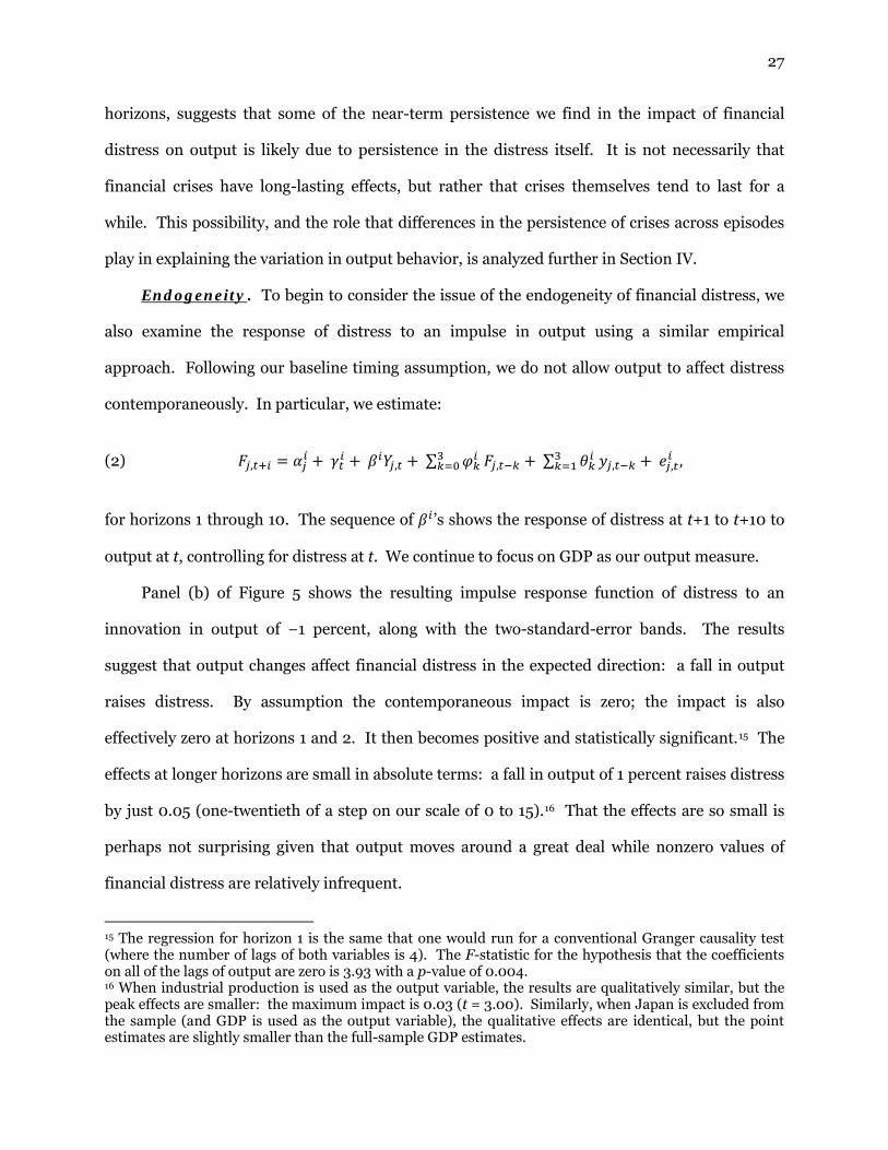
The particular specification that we estimate is:

(1) 𝑦𝑗,𝑡+𝑖 = 𝛼𝑗𝑖 + 𝛾𝑡𝑖 + 𝛽𝑖𝐹𝑗,𝑡 + ∑ 𝜑𝑘𝑖4

𝑘=1 𝐹𝑗,𝑡−𝑘 + ∑ 𝜃𝑘𝑖4𝑘=1 𝑦𝑗,𝑡−𝑘 + 𝑒𝑗,𝑡

𝑖 ,

where the j subscripts index countries, the t subscripts index time, and the i superscripts denote

the horizon (half-years after time t) being considered. yj,t+i is the log of output (either industrial

production or real GDP) for country j at time t+i. Fj,t is the financial distress variable for country

j at time t. We include four lags of both the distress variable and the output variable as

controls.13 We also include country fixed effects (the α’s) to capture the fact that normal output

behavior may differ across countries. Similarly, we include time fixed effects (the γ’s) to control

for economic developments facing all countries in a given year.

We estimate equation (1) for values of i from 0 to 10 half-years. That is, we consider

horizons up to five years after time t. The sequence of coefficients on the financial distress

variable at time t shows the behavior of output in response to an innovation in the distress

variable of 1. To make the interpretation of the impulse response function more

straightforward, we multiply the coefficients by 7, which is the value of our financial distress

measure corresponding to the start of the “moderate crisis” category. This transformed impulse

response function thus shows the behavior of output following a relatively large impulse in

13 Because we include four lags, the estimation begins in 1969:1. And because we do not want the behavior of output in the recent period to be driving the results, we do not use output data past 2007:1. The sample for horizon i therefore ends i half-years before 2007:1. For i = 4, for example, t runs from 1969:1 to 2005:1.

24

financial distress.

In the baseline estimates we include all 24 OECD countries for which we have the new

measure. As discussed above, a considerable fraction of the nonzero observations of financial

distress in our sample comes from Japan. Since this may give it an outsized weight in the

estimation, we also consider the 23-country sample excluding Japan. We consider a number of

additional variations of the baseline estimation in the subsection on robustness below.

B. Behavior of Output Following Financial Crises

We estimate equation (1) for the various horizons using both industrial production and real

GDP. Even at quite distant horizons, the sum of the coefficients on lagged output is close to one.

As a result, the country fixed effects essentially capture differences in average growth rates

across countries. The hypothesis that the country fixed effects are all zero is strongly rejected

for both output measures at all horizons (except the contemporaneous horizon for industrial

production). Similarly, the hypothesis that the time fixed effects are all zero is overwhelmingly

rejected for both output measures at all horizons.

Figure 3 shows the impulse response functions for the two output series estimated over the

full sample of 24 advanced countries, together with the two-standard-error bands. Panel (a)

shows the results for industrial production, and panel (b) for real GDP.

Industrial production falls noticeably at the time of the impulse to the financial distress

variable. The t-statistic on the contemporaneous relationship is over 4 (in absolute value). The

negative effect increases slightly in the half-year after the impulse. However, the absolute size of

the decline following a moderate crisis is modest: the peak effect is a decline of 3.9 percent (t =

–3.2). To put this number in perspective, Romer and Romer (1989) find that industrial

production fell roughly 12 percent following relatively exogenous shifts to contractionary

monetary policy in the United States in the postwar period. Another noteworthy feature of the

response of industrial production is how quickly the negative impact of a financial crisis

25

dissipates. The effect is a decline of just 1.7 percent (t = –1.2) within a year after the impulse and

zero within two years.

Real GDP also appears to decline contemporaneously with the impulse in the financial

distress variable. The immediate impact of a moderate crisis is a decline in GDP of 3.0 percent

(t = –6.1). This negative effect grows slightly over the 3½ years following the impulse, peaking

at 4.2 percent (t = –2.6). The striking difference between the responses of industrial production

and GDP is that the effects of a crisis on GDP appear to be much more persistent. Though the

standard errors increase substantially at longer horizons, the point estimate of the impact of a

moderate crisis is strongly negative for the full five years that we consider.

This persistence, however, is driven almost entirely by the case of Japan, which, as

described above, gets an outsized weight in the estimation. Japanese real GDP growth slowed

from over 4 percent per year to under 2 percent around the time that its extended financial

troubles began in the early 1990s, and then remained low. As a result, Japan’s experience points

strongly in the direction of financial distress having persistent negative long-run effects. Panel

(b) of Figure 4 shows the impulse response function for GDP when the sample excludes Japan.

The maximum fall in GDP following a moderate crisis is now 3.0 percent (t = –5.2), compared

with a decline of 4.2 percent in the full sample. More notable is the difference in persistence.

Without Japan in the sample, the estimated impact of a financial crisis on GDP begins to

dissipate after six months. By two years after the crisis, the point estimate is effectively zero.

After that, the point estimates turn positive, though the standard errors also become large.

Panel (a) of Figure 4 shows that excluding Japan also affects the estimated impulse

response function for industrial production. The effects of a moderate crisis, which are small in

the full sample, are now virtually nonexistent. The contemporaneous effect is a fall in industrial

production of just 2.5 percent (t = –2.5). The effect, which dissipates fairly quickly in the full

sample, goes away almost instantaneously in the no-Japan sample. By a year after the crisis, the

effect is positive; by two years after, the positive effect is actually significant.

26

The bottom line of the focal empirical results is that the relationship between output and

financial crises is not as dire as the modern conventional wisdom would lead one to believe, at

least in advanced countries. Using our new measure of financial distress and standard time-

series estimation methods, we find that the impact of a financial crisis on output is quite small.

And, with the exception of Japan, the impact does not appear to be very long-lasting. Indeed,

for industrial production, the negative effects are remarkably transitory.

C. Behavior of Financial Distress

The local projection approach to estimating the impulse response function for output does

not provide any information about the evolution and determinants of the distress variable itself.

However, it is straightforward to examine these issues.

The Persistence of Financial Distress. We first consider the response of the financial

distress variable to itself. Given our baseline timing assumption that output does not affect

distress within the period, the approach analogous to our method of estimating the output

effects is to estimate equation (1), replacing the left-hand-side variable with distress at t+i, 𝐹𝑗,𝑡+𝑖.

For i equal to zero, the coefficient is 1 by construction. We then estimate the equation for

horizons from 1 to 10 half-years after time t. We use GDP as the output control.

Panel (a) of Figure 5 shows the impulse response function of distress to itself, estimated

over the full sample of 24 countries. We again simulate the impact of an impulse of 7 in the

distress variable (a moderate crisis). The figure shows that there is important serial correlation

in financial distress. An impulse of 7 is followed by a value of the new measure of 5.9 a half-year

later. After two periods (1 year), the rate of decay speeds up noticeably, so that by 2½ years

after the impulse any effect of distress on itself is almost gone.14

That there is substantial serial correlation in the distress variable, particularly at near

14 We also estimate the impulse response function for the sample excluding Japan. Excluding Japan, where financial distress was extraordinarily persistent, results in a somewhat more rapid dying out of the impulse, but otherwise, the results are similar.

27

horizons, suggests that some of the near-term persistence we find in the impact of financial

distress on output is likely due to persistence in the distress itself. It is not necessarily that

financial crises have long-lasting effects, but rather that crises themselves tend to last for a

while. This possibility, and the role that differences in the persistence of crises across episodes

play in explaining the variation in output behavior, is analyzed further in Section IV.

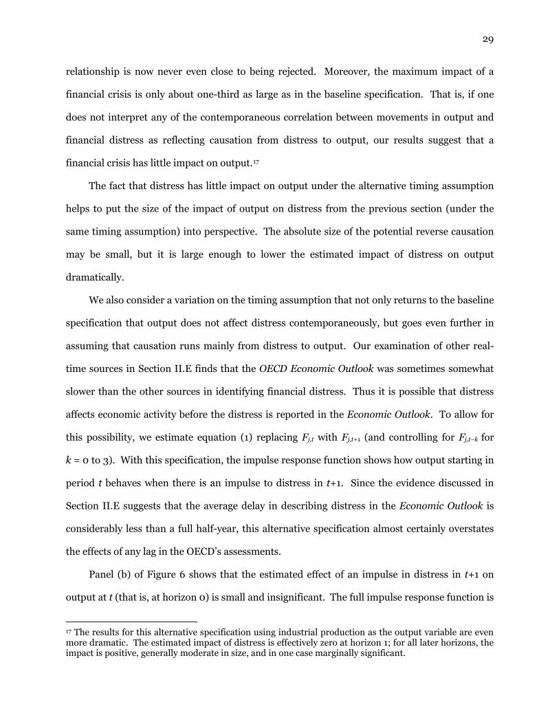
Endogeneity. To begin to consider the issue of the endogeneity of financial distress, we

also examine the response of distress to an impulse in output using a similar empirical

approach. Following our baseline timing assumption, we do not allow output to affect distress

contemporaneously. In particular, we estimate:

(2) 𝐹𝑗,𝑡+𝑖 = 𝛼𝑗𝑖 + 𝛾𝑡𝑖 + 𝛽𝑖𝑌𝑗,𝑡 + ∑ 𝜑𝑘𝑖3

𝑘=0 𝐹𝑗,𝑡−𝑘 + ∑ 𝜃𝑘𝑖3𝑘=1 𝑦𝑗,𝑡−𝑘 + 𝑒𝑗,𝑡

𝑖 ,

for horizons 1 through 10. The sequence of 𝛽𝑖’s shows the response of distress at t+1 to t+10 to

output at t, controlling for distress at t. We continue to focus on GDP as our output measure.

Panel (b) of Figure 5 shows the resulting impulse response function of distress to an

innovation in output of −1 percent, along with the two-standard-error bands. The results

suggest that output changes affect financial distress in the expected direction: a fall in output

raises distress. By assumption the contemporaneous impact is zero; the impact is also

effectively zero at horizons 1 and 2. It then becomes positive and statistically significant.15 The

effects at longer horizons are small in absolute terms: a fall in output of 1 percent raises distress

by just 0.05 (one-twentieth of a step on our scale of 0 to 15).16 That the effects are so small is

perhaps not surprising given that output moves around a great deal while nonzero values of

financial distress are relatively infrequent.

15 The regression for horizon 1 is the same that one would run for a conventional Granger causality test (where the number of lags of both variables is 4). The F-statistic for the hypothesis that the coefficients on all of the lags of output are zero is 3.93 with a p-value of 0.004. 16 When industrial production is used as the output variable, the results are qualitatively similar, but the peak effects are smaller: the maximum impact is 0.03 (t = 3.00). Similarly, when Japan is excluded from the sample (and GDP is used as the output variable), the qualitative effects are identical, but the point estimates are slightly smaller than the full-sample GDP estimates.

28

At the same time, the fact that the effects are small in absolute terms does not necessarily

imply that reverse causation is unimportant. To set the groundwork for further analysis of this

issue, we consider the response of distress to output, but with the alternative timing assumption

that output can affect distress contemporaneously. This is equivalent to estimating equation (1)

with roles of Y and F reversed, for horizons from 0 to 10. In this specification, the

contemporaneous effect of a 1 percent fall in output is a rise in distress of 0.05 (t = 6.14). The

effects at horizons 1 and 2 are roughly similar, and later effects are largely unchanged from those

in Figure 5b. Thus, even attributing all of the contemporaneous correlation between the two

series to an effect of output on distress yields a small estimate of the absolute impact.

D. Robustness

We examine the robustness of our findings along several dimensions. We discuss the most

important ones here; online Appendix C describes numerous others.

Alternative Timing Assumptions. One significant robustness check is to continue the

analysis of the alternative timing assumption that any contemporaneous relationship between

distress and output reflects the effect of output on distress. Under this assumption, the

appropriate way to find the response of output to distress is to estimate equation (2) with the

roles of Y and F reversed, for horizons from 1 to 10. With this change, the coefficient on Fj,t

shows the relationship between output in period t+i and the component of financial distress in

period t that is uncorrelated not just with financial distress and output before period t, but also

with output in period t.

Panel (a) of Figure 6 shows the estimated impulse response function of GDP to distress

under this timing assumption. This change sharply reduces the estimated effects of a financial

crisis. As before, we consider an impulse equal to 7 on our scale. By construction, the

contemporaneous effect of a financial crisis on output is now zero. The response at longer

horizons is consistently negative as in the baseline specification, but the null hypothesis of no

29

relationship is now never even close to being rejected. Moreover, the maximum impact of a

financial crisis is only about one-third as large as in the baseline specification. That is, if one

does not interpret any of the contemporaneous correlation between movements in output and

financial distress as reflecting causation from distress to output, our results suggest that a

financial crisis has little impact on output.17

The fact that distress has little impact on output under the alternative timing assumption

helps to put the size of the impact of output on distress from the previous section (under the

same timing assumption) into perspective. The absolute size of the potential reverse causation

may be small, but it is large enough to lower the estimated impact of distress on output

dramatically.

We also consider a variation on the timing assumption that not only returns to the baseline

specification that output does not affect distress contemporaneously, but goes even further in

assuming that causation runs mainly from distress to output. Our examination of other real-

time sources in Section II.E finds that the OECD Economic Outlook was sometimes somewhat

slower than the other sources in identifying financial distress. Thus it is possible that distress

affects economic activity before the distress is reported in the Economic Outlook. To allow for

this possibility, we estimate equation (1) replacing Fj,t with Fj,t+1 (and controlling for Fj,t–k for

k = 0 to 3). With this specification, the impulse response function shows how output starting in

period t behaves when there is an impulse to distress in t+1. Since the evidence discussed in

Section II.E suggests that the average delay in describing distress in the Economic Outlook is

considerably less than a full half-year, this alternative specification almost certainly overstates

the effects of any lag in the OECD’s assessments.

Panel (b) of Figure 6 shows that the estimated effect of an impulse in distress in t+1 on

output at t (that is, at horizon 0) is small and insignificant. The full impulse response function is

17 The results for this alternative specification using industrial production as the output variable are even more dramatic. The estimated impact of distress is effectively zero at horizon 1; for all later horizons, the impact is positive, generally moderate in size, and in one case marginally significant.

30

very similar to that in our baseline specification, but with a one-period delay.18

Overall, this analysis of alternative timing assumptions suggests that the baseline results

are likely to be a rough upper bound of the possible effects of distress on output. Even the

extreme assumption that output does not affect a lead of distress does not result in noticeably

larger estimated effects, and assuming that distress does not affect output contemporaneously

greatly reduces the estimated effects.

Possible Nonlinearities. A second significant robustness issue involves the scaling of

our distress variable. In constructing our measure, we attempted to choose the gradations so

that each step (such as credit disruption–regular to credit disruption–plus, or credit disruption–

plus to minor crisis–minus) is of roughly equal significance. However, since the descriptions in

the OECD Economic Outlook are qualitative rather than quantitative, we may not have been

completely successful in this effort. Moreover, even if each step is of equal importance in its

implications for the cost of credit intermediation, the response of economic activity to increases

in the cost of intermediation may not be linear.

As a simple way of shedding light on the possibility that the effects of financial distress are

nonlinear in our measure, F, we estimate a variant of our baseline specification that allows the

effects of distress to be quadratic in F. In this estimation, we use the baseline assumption that

distress can affect output contemporaneously (but output cannot affect distress within the

period). We then estimate the system of equations:

(3) 𝑦𝑗,𝑡+𝑖 = 𝛼𝑗𝑖 + 𝛾𝑡𝑖 + 𝛽𝑖𝑓�𝐹𝑗,𝑡� + ∑ 𝜑𝑘𝑖4

𝑘=1 𝑓�𝐹𝑗,𝑡−𝑘� + ∑ 𝜃𝑘𝑖4𝑘=1 𝑦𝑗,𝑡−𝑘 + 𝑒𝑗,𝑡

𝑖 ,

with 𝑓(𝐹) = 𝐹 + 𝑏𝐹2. b > 0 corresponds to the case where the gaps between successive steps of

our distress measure increase as one moves up the scale, or where the output effects of equal

increases in distress rise as distress rises. b < 0 corresponds to the opposite case. Our baseline

18 When industrial production is used as the output measure, the effect at horizon 0 is again small and insignificant. The full impulse response function is similar to that in the baseline (with a one-period delay), but shows slightly larger negative effects.

31

specification corresponds to the case b = 0. We estimate (3) using nonlinear least squares. For

simplicity, we focus on the results using GDP as the output measure.

The results suggest little nonlinearity. The estimate of b is –0.025 with a standard error of

0.017. Thus, the null hypothesis that the linear specification is correct cannot be rejected.

Moreover, the point estimate implies that the variation across categories is only slightly different

from what we assume in our baseline scaling. For example, in our baseline scaling, a regular

moderate crisis is 4 times as consequential as a regular credit disruption (8 versus 2); in the

quadratic specification, it is 3.4 times as consequential (8 – 0.025(82) versus 2 – 0.025(22)).19

Other Robustness Issues. Appendix C discusses numerous other robustness checks of

the baseline results. We examine alternative specifications, such as a single-equation

autoregressive model, a standard vector autoregression, a less parametric way of allowing for

nonlinearity, and including country-specific trends. We also consider various alternative

samples of both time periods and countries. Finally, we discuss correcting the standard errors

for possible heteroskedasticity and serial correlation. The results in Appendix C show that none

of these permutations make the estimated effects of financial distress on output substantially

larger or more persistent. Indeed, a few of the changes make the effects noticeably weaker.

E. Comparison with Results Using Alternative Chronologies

Given that our new series on financial distress differs in important ways from existing

crisis chronologies, it is useful to compare our findings for the output response with ones

estimated using the other series. As in Section II, we consider both the Reinhart and Rogoff

(2009a) chronology and the dates from the IMF database. We again only consider the

alternative chronologies for the 24 advanced countries in our sample. To incorporate the

19 When we use industrial production as the output measure, the estimate of b is 0.15 with a standard error of 0.15. Thus, the null hypothesis that the linear specification is correct is again not close to being rejected. In this case, however, the point estimate suggests that the gaps between successive steps of our distress measure increase slightly rather than decrease slightly as one moves up the scale. For example, it implies that a regular moderate crisis is 6.8 times as consequential as a regular credit disruption, rather than 4 times as consequential.

32

alternative chronologies into the empirical framework used above, we simply convert each to a

dummy variable equal to 1 in all half-years from the start to the end of a crisis in a given country,

and 0 otherwise. This allows us to create a panel dataset similar to that created using our new

continuous measure of financial distress.

We estimate equation (1) for various horizons using each of the alternative crisis series in

place of our financial distress variable (the F terms).20 The resulting impulse response functions

show the effect of a realization of a 1 in the alternative chronology. Since the impulse response

functions we show for our new series are for a realization of a 7 on our scale from 0 to 15 (a

moderate crisis–minus), the experiments considered are roughly comparable.

The impulse response functions for real GDP for both alternative crisis measures are

shown in Figure 7. Panel (a) shows that GDP falls much more slowly when the Reinhart and

Rogoff crisis series is used instead of the new series. There is almost no response in the

contemporaneous half-year, and the impact builds gradually over the next year and a half. Panel

(b) shows that the response of GDP to the IMF crisis variable is substantially faster than that

estimated using the Reinhart and Rogoff series, but still more gradual than when our new

measure is used. With the IMF series, the contemporaneous impact is about one-third of the

maximum impact and only marginally significant. With the new series, the contemporaneous

impact is three-quarters of the maximum, and highly significant.

The difference in the speed of response is unsurprising given the comparison of the various

series in major episodes shown in Figure 2. Reinhart and Rogoff date crises much earlier than

does the new series. Similarly, the IMF chronology also dates crises somewhat before the new

series, and typically well before the new series shows an acute rise. The consideration of

additional real-time evidence in Section II.E suggests that the new measure may sometimes be

slightly late in registering distress. Thus, the actual speed of response of GDP to distress may lie

20 For the Reinhart and Rogoff series, the data are for 1967:1–2006:2; for the IMF series, they are for 1970:1–2006:2.

33

between the results for the new measure and that for the alternative chronologies.

Another feature of the impulse response function estimated using the Reinhart and Rogoff

crisis series is that the maximum impact is remarkably small. Following a crisis, real GDP falls

only 2.3 percent.21 This is noticeably less than the 4.2 percent fall we find following a moderate

crisis in our new series. The maximum fall using the IMF series is 3.3 percent.

The small response of GDP in advanced countries that we find using the Reinhart and

Rogoff crisis series stands in stark contrast to the usual summary of Reinhart and Rogoff as

showing that the recessions following financial crises are particularly severe. Indeed, Figure

14.4 of This Time is Different (2009a, p. 230) shows that the average peak-to-trough decline in

real GDP per capita in a sample of crises is 9.3 percent.

Much of the smaller effect we find using Reinhart and Rogoff’s crisis dates in our empirical

framework is due to the fact that we are only considering crises in advanced economies in the

post-1967 period. Most of the large declines behind that 9.3 percent average come from postwar

crises in emerging economies (such as Argentina, Thailand, and Indonesia, where the declines in

output per capita were well over 10 percent) and from one crisis before World War II (the U.S.

Great Depression, where the peak-to-trough decline in per capita GDP was close to 30 percent).

Some of the difference also reflects the fact that we are considering the full universe of crises

that Reinhart and Rogoff identify in the 24 OECD countries after 1967. The 9.3 percent is the

average decline in a selected set of severe episodes. Finally, some of the difference reflects our

regression-based empirical approach. Reinhart and Rogoff’s measure of the peak-to-trough

decline in GDP per capita around crises often includes falls that predate the crisis. For example,

in Finland, where the fall in output was very large, most of the decline occurred before the onset

of significant banking problems. In contrast, the regression procedure only looks at the

behavior of output following the crises.22

21 The results using the Reinhart and Rogoff chronology are very similar if we use the dates from the website for Reinhart and Rogoff (2009a) instead of those from Table A.4.1 in the book. 22 In converting both the Reinhart and Rogoff and the IMF crisis dates into a dummy variable, we set the

34

A third feature of the impulse response functions for GDP using the alternative

chronologies involves the persistence of the decline. Recall that for the new series using the full

sample, the decline in GDP following a crisis is quite persistent. The same is true following a

crisis in the Reinhart and Rogoff series. In contrast, using the IMF series, there is substantial

bounce back: two-thirds of the GDP decline is reversed within five years after the start of the

crisis.

In the results using the new series, the persistence of the effect of a crisis on GDP is due

entirely to the case of Japan. Japan had a very prolonged period of financial distress, and so the

large slowdown in GDP growth in Japan after 1990 gets a great deal of weight in the estimation.

When Japan is excluded, the GDP effects disappear within two years. In contrast, the results

using the Reinhart and Rogoff series are not very sensitive to the inclusion of Japan. In their

non-scaled series with many crises, Japan gets only a small weight, so excluding it matters

relatively little. For the IMF series, excluding Japan lessens the maximum GDP decline in the

impulse response function by about 20 percent, and causes the effect to go away entirely after

five years. This happens even though the series is not scaled because there are only eight crises

in advanced economies in the period 1970 to 2006 in the IMF chronology—so the experience of

Japan is still getting substantial weight in the full-sample estimates.

The bottom line of the results using alternative crisis chronologies is that for no crisis

measure is the estimated impact of severe financial distress very large. Using standard

regression techniques on the same sample of advanced economies since 1970 shows quite minor

effects on output. Financial crises just do not seem to be followed by large declines in output in

crisis dummy equal to 1 in all half-years for which the chronology indicates that a country was experiencing a crisis. An alternative is to set it equal to 1 only in the half-year corresponding to the start of the crisis. When we use this alternative in the estimation, the impact of a crisis is slightly more negative and slightly less precisely estimated. For example, using the IMF chronology, the impact on GDP in the full sample after five half-years is –3.3 percent (s.e. = 1.1) for the full dummy and –3.8 percent (s.e. = 1.6) for the start-only dummy. Both of these differences make sense. The fall in GDP at the start of a crisis tends to be sharper than the rise when the crisis ends. As a result, including late phases of a crisis in the dummy leads to smaller estimated negative impacts. Looking only at the start of crises discards information about how long crises last. Thus, it would be surprising if the standard errors did not rise when the start-only dummy is used.

35

advanced economies in the modern period, whichever chronology is used.23

Nevertheless, there are interesting differences across the results for the various crisis

measures. Using our new measure of financial distress, the impact of crises appears to be much

faster than when the alternative crisis measures are used. Also, when Japan is excluded from

the sample, any impacts of crises appear to be much less persistent when the new measure of

financial distress is used. Thus, using the new measure challenges the notion that the effects of

crises are particularly long-lasting.

IV. VARIATION IN THE AFTERMATH OF FINANCIAL CRISES ACROSS EPISODES

So far, we have used our new measure of financial distress in modern advanced economies

to examine the usual relationship between financial crises and economic activity. We turn now

to the question of how that relationship varies across episodes.

A. Analysis of Key Episodes

To investigate the variation across episodes, we focus on the cases where there was the

most significant financial distress. Specifically, we look at all of the cases where our new

measure reached at least 7 on our scale. There are seven of these: Finland in 1993:1; Japan in

1997:2 and again in 2002:1; Norway in 1991:2; Sweden in 1993:1; Turkey in 2001:1, and the

United States in 1990:2. For simplicity, we treat the two Japanese crises as a single episode

beginning in 1997:2.

23 That the effects of crises in advanced countries using the Reinhart and Rogoff and IMF chronologies are modest is somewhat surprising given that Cerra and Saxena (2008) find large effects using a simple autoregressive specification and the Caprio and Klingebiel (2003) crisis dates that were the precursor to both of these later alternatives. Some of the difference is surely due to the specific crisis dates used; the current IMF series, in particular, modifies the Caprio and Klingebiel dates substantially. But some of the difference is due to the empirical specification. Cerra and Saxena do not include time fixed effects in their regressions, but all of our specifications do (and the F-tests indicate strongly that they are important). Omitting time fixed effects leads to substantially larger estimates of the fall in output following crises. Also, in our baseline specification for the alternative chronologies, we use a dummy variable equal to 1 in all half-years when there was a crisis; Cerra and Saxena use a dummy equal to 1 only at the start of a crisis. Though this difference in specification has little impact when the Jordà approach is used, it matters more in the one-equation autoregressive specification used by Cerra and Saxena—mainly through its effect on the experiment simulated.

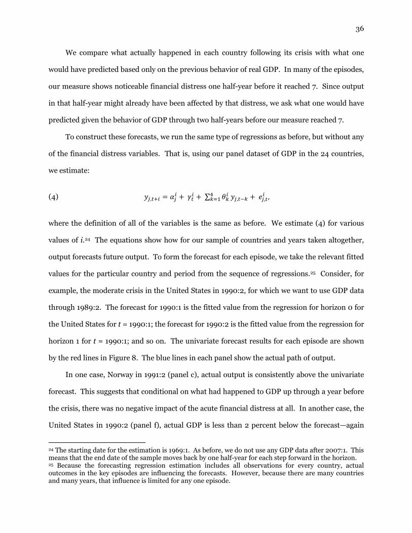
36

We compare what actually happened in each country following its crisis with what one

would have predicted based only on the previous behavior of real GDP. In many of the episodes,

our measure shows noticeable financial distress one half-year before it reached 7. Since output

in that half-year might already have been affected by that distress, we ask what one would have

predicted given the behavior of GDP through two half-years before our measure reached 7.

To construct these forecasts, we run the same type of regressions as before, but without any

of the financial distress variables. That is, using our panel dataset of GDP in the 24 countries,

we estimate:

(4) 𝑦𝑗,𝑡+𝑖 = 𝛼𝑗𝑖 + 𝛾𝑡𝑖 + ∑ 𝜃𝑘𝑖4

𝑘=1 𝑦𝑗,𝑡−𝑘 + 𝑒𝑗,𝑡𝑖 ,

where the definition of all of the variables is the same as before. We estimate (4) for various

values of i.24 The equations show how for our sample of countries and years taken altogether,

output forecasts future output. To form the forecast for each episode, we take the relevant fitted

values for the particular country and period from the sequence of regressions.25 Consider, for

example, the moderate crisis in the United States in 1990:2, for which we want to use GDP data

through 1989:2. The forecast for 1990:1 is the fitted value from the regression for horizon 0 for

the United States for t = 1990:1; the forecast for 1990:2 is the fitted value from the regression for

horizon 1 for t = 1990:1; and so on. The univariate forecast results for each episode are shown

by the red lines in Figure 8. The blue lines in each panel show the actual path of output.

In one case, Norway in 1991:2 (panel c), actual output is consistently above the univariate

forecast. This suggests that conditional on what had happened to GDP up through a year before

the crisis, there was no negative impact of the acute financial distress at all. In another case, the

United States in 1990:2 (panel f), actual GDP is less than 2 percent below the forecast—again

24 The starting date for the estimation is 1969:1. As before, we do not use any GDP data after 2007:1. This means that the end date of the sample moves back by one half-year for each step forward in the horizon. 25 Because the forecasting regression estimation includes all observations for every country, actual outcomes in the key episodes are influencing the forecasts. However, because there are many countries and many years, that influence is limited for any one episode.

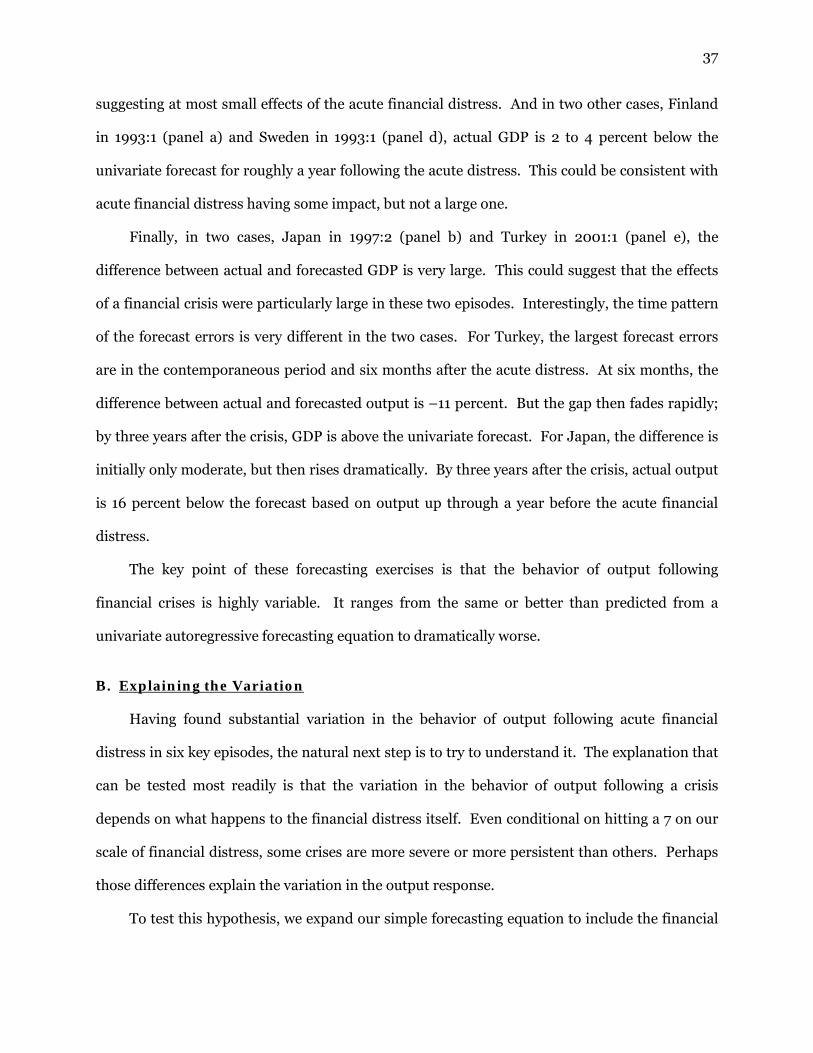
37

suggesting at most small effects of the acute financial distress. And in two other cases, Finland

in 1993:1 (panel a) and Sweden in 1993:1 (panel d), actual GDP is 2 to 4 percent below the

univariate forecast for roughly a year following the acute distress. This could be consistent with

acute financial distress having some impact, but not a large one.

Finally, in two cases, Japan in 1997:2 (panel b) and Turkey in 2001:1 (panel e), the

difference between actual and forecasted GDP is very large. This could suggest that the effects

of a financial crisis were particularly large in these two episodes. Interestingly, the time pattern

of the forecast errors is very different in the two cases. For Turkey, the largest forecast errors

are in the contemporaneous period and six months after the acute distress. At six months, the

difference between actual and forecasted output is –11 percent. But the gap then fades rapidly;

by three years after the crisis, GDP is above the univariate forecast. For Japan, the difference is

initially only moderate, but then rises dramatically. By three years after the crisis, actual output

is 16 percent below the forecast based on output up through a year before the acute financial

distress.

The key point of these forecasting exercises is that the behavior of output following

financial crises is highly variable. It ranges from the same or better than predicted from a

univariate autoregressive forecasting equation to dramatically worse.

B. Explaining the Variation

Having found substantial variation in the behavior of output following acute financial

distress in six key episodes, the natural next step is to try to understand it. The explanation that

can be tested most readily is that the variation in the behavior of output following a crisis

depends on what happens to the financial distress itself. Even conditional on hitting a 7 on our

scale of financial distress, some crises are more severe or more persistent than others. Perhaps

those differences explain the variation in the output response.

To test this hypothesis, we expand our simple forecasting equation to include the financial

38

distress variable up through the horizon of the output variable. That is, we estimate:

(5) 𝑦𝑗,𝑡+𝑖 = 𝛼𝑗𝑖 + 𝛾𝑡𝑖 + ∑ 𝜑𝑘𝑖𝑖

𝑘=−4 𝐹𝑗,𝑡+𝑘 + ∑ 𝜃𝑘𝑖4𝑘=1 𝑦𝑗,𝑡−𝑘 + 𝑒𝑗,𝑡

𝑖 .

As before, we estimate the regression for various values of i. To form the forecasts for each

episode, we take the relevant fitted values from the sequence of regressions. Because the

financial distress variable has the same horizon as the output variable, we are using the actual

evolution of the distress variable in the prediction. As before, we only use output up through a

year before our measure reached 7.

The green line in each panel of Figure 8 shows the forecast including the actual path of the

financial distress variable. The results suggest that the severity or persistence (or both) of the

financial distress explains much of the discrepancy between the simple univariate forecast of

output and what actually happened in the key episodes.

The most striking case is Japan (panel b). The green and blue lines are very close for the

first year following the distress variable reaching 7. That is, the forecast including the actual

realizations of the distress variable matches actual GDP closely. After a year, the two diverge.

But then the forecast including the actual evolution of the distress variable falls again and

remains anemic, concurrent with the second bout of acute distress in Japan in the early 2000s.

After 5 years, the forecast including the actual evolution of the distress variable deviates from

actual GDP behavior by only about one-quarter as much as the forecast based on output alone.

This suggests that much of Japan’s dismal economic performance following its initial bout of

acute financial distress is related to the fact that the distress was particularly severe and long-

lasting. At the same time, the shortfall of GDP from the forecast that includes the actual path of

distress remains substantial in absolute terms.

For both Finland and Sweden (panels a and d), where the univariate forecast and actual

GDP are moderately different, including the evolution of financial distress again brings the

forecast much closer to the actual series, both in the near term and at longer horizons. Indeed,

39

for Finland, the forecast including the evolution of distress is virtually identical to actual output.

For Turkey (panel e), the forecast including the actual evolution of the financial distress

variable is certainly closer to the actual behavior of GDP than is the forecast based only on

lagged output. The forecast error in the first half-year after the onset of acute distress falls from

–11 percent to –7 percent. However, that a very large discrepancy remains suggests that factors

other than acute financial distress played a role in this episode. For example, the fact that

Turkey’s financial crisis was accompanied by a severe currency crisis may have exacerbated the

output decline. Turkey is also one of the least advanced economies in our sample. It is possible

that financial crises have larger impacts or that real GDP is simply more volatile in less

developed economies.

For the United States (panel f), the forecast including the actual evolution of distress is

substantially worse than what actually happened. That is, including distress more than

eliminates the univariate forecast error. At the same time, in the year following the acute

distress, the expanded forecast is closer to actual output than the univariate forecast, suggesting

that the evolution of distress may explain some of the unusual behavior of output in the United

States in this period.

Finally, for Norway, where the univariate forecast is consistently below actual output,

including the actual evolution of distress makes the forecast errors even larger. Based on the

fact that Norway had a relatively severe panic, with a second acute phase a year after the first,

the forecast including the evolution of the distress variable is quite weak for nearly two years.

Yet actual output barely paused. This suggests that the behavior of distress provides little

insight into the behavior of the Norwegian economy in this period.

The bottom line of the analysis of this section is that there is substantial variation in the

behavior of output following financial distress. The severity and persistence of this distress in

particular episodes appears to explain much, but certainly not all, of this variation.

40

V. CONCLUSION

The conventional wisdom has become that financial crises are followed by large downturns

and weak recoveries. Yet at least for advanced countries, the prior evidence supporting this

conclusion is limited. It is based on chronologies for crises that differ substantially from one

another; that were constructed after-the-fact, often using imprecise criteria; and that simplify a

continuum of possible degrees of financial distress to a 0-1 variable or just a handful of

categories. Moreover, the conclusions about the aftermath of crises are typically based on

samples dominated by crises in developing countries or in the prewar era; and they are often

derived using relatively simple empirical techniques, such as comparisons of recessions with and

without crises.

Findings. This paper therefore revisits the aftermath of financial crises in advanced

countries in the postwar era. We construct a new financial distress series for 24 countries from

1967 to 2007 using accounts of member country conditions prepared twice a year by the OECD.

Our new series classifies financial distress into numerous gradations, which we scale from 0 to

15.

The new series displays both important similarities and important differences with

previous crisis chronologies. There is agreement about the presence and approximate timing of

many of the most severe crises. But the timing of distress in the new measure sometimes differs

substantially from the dates identified in earlier chronologies. In addition, the new series often

shows important variation over time within episodes in the severity of distress; by construction,

other chronologies do not show such variation. Finally, a few episodes that previous series

identify as important crises do not show up at all in our new measure. Analysis of three other

real-time sources largely confirms the accuracy of the new series.

Studying the aftermath of crises using our new series and standard regression techniques

leads to a view that is very different from the conventional wisdom. Crises in advanced

countries are associated with falls in output, but the falls are only moderate. When measured

41

using industrial production, output quickly rebounds and returns to its pre-crisis path. When

measured using GDP, output does not bounce back, but this pattern is driven entirely by the

experience of Japan. Interestingly, these findings are due only partly to our new measure of

financial distress. Using conventional regression techniques with previous chronologies of

postwar financial crises in advanced countries also does not provide strong support for the view

that the aftermaths of crises are persistently grim.

We also find considerable variation in the aftermath of significant crises. In some cases,

there was hardly any departure of output from its pre-crisis path. In others, output fell below

the pre-crisis path but was soon noticeably above it. And in the case of Japan in the late 1990s,

output fell further and further below the pre-crisis path. One factor that appears to be

important to the variation is the severity and persistence of the crisis itself. Cases where the

financial distress was more limited and resolved quickly were associated with more favorable

outcomes.

Understanding the Aftermath of the 2008 Crisis. Our study was motivated in part

by a desire to understand the experience following the 2008 financial crisis. Why was the

downturn in 2008–2009 so extreme and the subsequent recovery so anemic in many advanced

countries? Our finding that the fall in output following financial crises in such countries is

typically modest suggests that the easy explanation for the poor economic performance—this is

what always happens after a financial crisis—is unlikely to be true. Rather, factors specific to the

2008 episode are likely to have been key.

The factor most directly linked to our results involves the severity and persistence of the

recent financial distress. The 2008 crisis was the worst in nearly a century in the United States

and Europe. And, although it has been over half a decade since the acute phase of the crisis,

banks in many European countries are still viewed as troubled and as constraining the

availability of credit. Since we find that greater severity and persistence of financial distress is

associated with worse performance following a crisis, the extreme nature of the recent distress is

42

one likely reason for the severe and continuing economic weakness.

A related factor is that the recent financial crisis was essentially worldwide, while other

postwar episodes of severe financial distress were limited to individual countries or narrow

regions. When a crisis is confined to a single country or to just a few, healthy financial

institutions abroad may offset some of the reduction in credit supply from domestic lenders. A

worldwide crisis means that there are few healthy lenders to step into the void. More generally,

a crisis in one country may have adverse spillovers to others. One would therefore expect a

given rise in domestic financial distress to be associated with worse outcomes when distress also

increases in other countries.

While the greater severity and worldwide nature of the financial distress may be part of the

explanation for the terrible aftermath of the 2008 crisis, there are other possibilities. For

example, the period before the crisis witnessed large housing booms and accumulations of

household debt in many major countries. Mian and Sufi (2014) argue that these developments,

rather than the financial crisis itself, were the main drivers of the downturn and, especially, of

the weak recovery. Similarly, worldwide fiscal retrenchment may have played a role. The shifts

to tighter fiscal policy that began in continental Europe in late 2009 and early 2010, the United

Kingdom in 2010, and the United States in 2011 cannot explain the severity of the downturn, but

they may have been important to the slow recovery.

Finally, the zero lower bound on nominal interest rates may have exacerbated the effects of

the recent financial crisis. Central banks in advanced countries often respond to financial

distress by reducing their policy rates. But those rates have been at or near zero in most major

advanced countries since 2009. The constraint on this usual cushioning mechanism may have

magnified the effects of the financial crisis. This possibility is consistent with our finding that,

even accounting for the actual behavior of financial distress, Japan’s output performance

following its crisis was worse than would have been predicted. Japan’s policy rate has been

close to zero almost without interruption since shortly after the peak of its financial crisis in the

43

late 1990s, and it is the only country in our sample that encountered the zero lower bound in the

period we consider.

Limitations and Questions for Further Study. In many ways, our findings raise

more questions than they answer. With respect to the recent episode, much research is needed

to determine if one of the possibilities mentioned above, a combination of those factors, or

something else explains the poor economic performance of advanced countries since 2008.

With respect to the effects of crises more generally, one important limitation of previous

work that our paper does not address involves the issue of causation. Lower output is likely to

weaken financial institutions and so contribute to financial distress, and there may be factors

that cause both higher distress and lower output. As a result of this omitted variable bias, the

correlation between distress and output estimated in our baseline specification is likely to

overstate the adverse effect of crises. One indication that the overstatement may be

considerable is that essentially all of the relationship between distress and output that we find

arises from the contemporaneous relationship. Isolating the causal effects of crises is a

challenging and important topic for future work.

Another limitation of our analysis is that it only looks at the experience of advanced

countries. This may in fact be a virtue if the response of advanced countries to financial distress

is different from that in developing countries. At the same time, it means that our results do not

provide any direct information about the impact of financial distress in emerging economies.

Importantly, such issues as difficulties in the identification of crises and complications arising

from the use of simple summary statistics may also be relevant to investigations of the aftermath

of financial crises in developing countries. Indeed, because output in developing countries is

generally more volatile and the data are typically of lower quality, these problems could be even

more serious in that setting. Thus, addressing these concerns for developing countries is

another important area for future research.

In addition, we consider only one source of variation in the aftermath of crises—differences

44

in the severity and persistence of the financial distress itself. As suggested in the case of the

2008 crisis, many other factors may play a role. Thus another valuable area for future research

is identifying and determining what else might explain the variation in the effects of distress

across episodes.

Finally, there is still a great deal that we need to understand about the role of policy. In the

conventional view that the aftermath of financial crises is uniformly awful, the policy focus is

naturally just on preventing crises. But our finding that there is substantial variation in

outcomes suggests different questions. Are there policies that can be undertaken in normal

times not just to reduce the chances of crises, but to make their consequences less grave if they

occur? What policy actions when a crisis occurs—in addition to steps to lessen the crisis and

resolve it quickly—could minimize its effects? The answers to these questions are important for

ensuring not just that each time is different, but that none is terrible.

45

TABLE 1 Financial Distress in OECD Countries, 1967:1–2007:1

Finland Japan (continued) 1992:1 Credit disruption–regular 1999:1 Moderate crisis–plus 1992:2 Minor crisis–plus 1999:2 Minor crisis–plus 1993:1 Moderate crisis–regular 2000:1 Minor crisis–minus 1993:2 Minor crisis–regular 2000:2 Credit disruption–plus 1994:1 Credit disruption–plus 2001:1 Minor crisis–plus 2001:2 Minor crisis–plus France 2002:1 Moderate crisis–regular 1991:2 Credit disruption–minus 2002:2 Moderate crisis–minus 1995:1 Credit disruption–regular 2003:1 Minor crisis–plus 1995:2 Minor crisis–minus 2003:2 Minor crisis–regular 1996:1 Minor crisis–regular 2004:1 Minor crisis–minus 1996:2 Minor crisis–regular 2004:2 Credit disruption–plus 1997:1 Credit disruption–plus 2005:1 Credit disruption–regular Germany Norway 1974:2 Credit disruption–regular 1991:2 Moderate crisis–plus 2003:1 Credit disruption–minus 1992:1 Minor crisis–regular 1992:2 Moderate crisis–regular Iceland 1993:1 Minor crisis–plus 2006:2 Minor crisis–regular 1993:2 Credit disruption–plus 2007:1 Credit disruption–regular 1994:1 Credit disruption–regular Italy Sweden 1997:1 Credit disruption–minus 1992:2 Minor crisis–regular 1993:1 Moderate crisis–regular Japan 1990:2 Credit disruption–plus Turkey 1991:1 Credit disruption–minus 2001:1 Moderate crisis–regular 1991:2 Minor crisis–regular 2001:2 Moderate crisis–regular 1992:1 Credit disruption–plus 2002:1 Minor crisis–plus 1992:2 Minor crisis–minus 2002:2 Minor crisis–minus 1993:1 Minor crisis–minus 2003:1 Minor crisis–minus 1993:2 Minor crisis–regular 2003:2 Credit disruption–regular 1994:1 Credit disruption–plus 1994:2 Credit disruption–plus United States 1995:1 Minor crisis–minus 1986:1 Credit disruption–minus 1995:2 Minor crisis–regular 1990:1 Minor crisis–regular 1996:1 Minor crisis–plus 1990:2 Moderate crisis–regular 1996:2 Minor crisis–minus 1991:1 Minor crisis–minus 1997:1 Minor crisis–regular 1991:2 Credit disruption–plus 1997:2 Moderate crisis–minus 1992:1 Credit disruption–regular 1998:1 Major crisis–regular 1998:2 Credit disruption–plus 1998:2 Extreme crisis–minus 2007:1 Credit disruption–minus Notes: Based on the OECD Economic Outlook. The Economic Outlook does not describe any disruptions or crises in Australia, Austria, Belgium, Canada, Denmark, Greece, Ireland, Luxembourg, Netherlands, New Zealand, Portugal, Spain, Switzerland, and the United Kingdom. The sample period is 1967:1–2007:1 for all countries except Australia (1971:2–2007:1), Finland (1969:1–2007:1), and New Zealand (1973:1–2007:1). Countries that joined the OECD after 1993 are not considered.

46

EXHIBIT 1 Sample Descriptions of Episodes from Online Appendix A

A. Credit Disruption–Regular

Germany, 1974:2. The OECD reported that during the summer, “considerable losses of exchange reserves and the imminent danger of a confidence crisis imposed particular strains on the banking system,” and that “[s]pecial credit facilities were extended to small and medium-sized companies and reserve requirements were reduced in September and October” (p. 26; see also p. 51). And in a discussion of Germany, the United Kingdom, and the United States, it stated, “Recent strains on the banking system in all three countries have underlined the unfavourable climate in bank lending markets. … There is evidence in all three countries that smaller companies have been particularly severely rationed or priced out of bank lending markets” (p. 50). Notably, there was no mention of financial-market difficulties in the section that was specifically devoted to Germany. Given that omission, it is clear that the OECD did not view financial-market problems as being a major factor in the behavior of the German economy. On the other hand, it identified strains on the banking system, and Germany had perceived a need for special facilities to support lending to certain types of businesses.

This disruption seems similar to that in the United States in 1992:1 (which we classify as a regular

credit disruption), and less serious than that in the United States in 1991:2 (which we classify as a credit disruption–plus). We code this episode as a credit disruption–regular. B. Minor Crisis–Regular

France, 1996:1. The OECD reported (p. 78): In 1995, the banking sector continued to suffer from low credit demand, high refinancing and operating costs and large provisions for bad debts. As a result, profitability has been very low by international comparison. The State has provided financial support to some banks and insurance companies, and several financial companies have created special corporate structures in order to assure that prudential ratios are higher than required. Lower short-term interest rates will reduce refinancing costs and help the financial sector to restore profitability. However, the current level of provisions still does not cover all doubtful credits as the real estate market has softened again and the restructuring of the banking sector is advancing only slowly.

The combination of the significant problems in the banking sector, the statement that banks faced high refinancing costs, and the fact that the banking problems were not given a central role in the OECD’s discussion of the outlook causes us to identify this episode as a minor crisis–regular. This classification is consistent the fact that we classify France in 1995:2 as a minor crisis–minus, and that the description of the health of the banking sector in this issue is slightly more negative. C. Moderate Crisis–Regular

Sweden, 1993:1. In the summary of its entry, the OECD said, “Steeply falling property values have led to a sharp increase in corporate bankruptcies and heavy loan losses in banks’ balance sheets” (p. 113). A paragraph devoted to the financial system reported (p. 115):

Falling asset values and corporate bankruptcies linked to the collapse in the commercial

property market have provoked an unprecedented increase in banks’ loan losses. These reached Skr 70 billion in 1992 (7.7 per cent of outstanding loans), up from Skr 36 billion in 1991. Losses are widely expected to remain high in 1993. With the capital bases of most major

47

banks rapidly eroding, the Government has guaranteed that banks can meet their commitments. Government rescue operations are officially estimated to burden the 1992/93 budget by Skr 22 billion (1½ per cent of GDP), with off-budget loans and guarantees amounting to an additional Skr 46 billion (over 3 per cent of GDP). It is not known what scale of rescue operations will be needed in the 1993/94 budget.

Finally, in discussing risks to the outlook, the OECD stated, “greater weakness of demand could be accentuated by rising capital costs in the event of larger loan losses. This would … risk reducing credit supply” (p. 115).

This episode is similar to Norway in 1992:2 and Finland in 1993:1. The most obvious difference is

that in this case, the OECD devoted a sentence in its summary to the financial-market problems. But the financial system was starting from a slightly better position than Finland’s was (as described above, we code Sweden in 1992:2 as a minor crisis–regular, whereas we classify Finland in 1992:2 as a minor crisis–plus). And, in contrast to the discussion of Norway, there was no explicit reference to firms facing difficulties in obtaining financing. We therefore also classify this episode as a moderate crisis–regular. D. Extreme Crisis–Minus

Japan, 1998:2. As just discussed, we classify Japan in 1998:1 as a major crisis–regular. Here, the OECD described a situation that was notably worse. Among its stronger phrases were “financial paralysis” (p. 20); the “breakdown in the credit creation mechanism, and the resulting widening of creditor risk premia” (p. 44); “banks remain in dire straits as risk premia widen” (p. 45); “the increasingly serious situation in the banking sector” (p. 45); and “credit crunch” (which it used repeatedly). In addition, it discussed major government interventions in the financial system: “a broad agreement was achieved in the Diet to revitalise the financial system. The new legislation includes important measures to deal with financial sector problems. To support this, the Government has made an unprecedentedly large sum of public funds available to recapitalize the banking system, amounting overall to around ¥ 60 trillion, or about 12 per cent of GDP” (p. ix).

The OECD made it clear that those developments were having an important impact on the economy.

For example, it said, “a profound lack of confidence, in large part due to the severe and prolonged crisis in the banking system, has depressed private spending” (p. 20); reported that “the balance sheet problems of the banking sector remain unresolved, and the resulting uncertainty has led to diminished confidence among consumers and investors, leading to sharp declines in private spending” (p. 42); and referred to “risks of a deflationary spiral arising in part from the unresolved problems in the banking sector” (p. 44).

However, although there had clearly been a nontrivial deterioration from 1998:1, the OECD did not

describe the situation as qualitatively changed. For example, it said, “banking sector problems were not improving” (p. ix), and referred to “continued concerns about the health of the financial system” (p. 12). And in the summary of its entry, it stated, “The credit crunch is continuing” (p. 42). Also, as noted above, it commented that “banks remain in dire straits” (p. 45).

Thus, the financial-sector problems had become significantly but not dramatically worse. We

therefore classify this episode as two steps more serious than in 1998:1, which corresponds to an extreme crisis–minus.

48

FIGURE 1 New Measure of Financial Distress for Advanced Countries

Notes: See text and Appendix A for details about the derivation of the new measure. The data are available semiannually from 1967:1 to 2007:1. The figure only shows the data for the ten OECD countries that had some nonzero values of our measure. In the new measure, 0 corresponds to no financial distress; 1, 2, and 3 correspond to gradations of credit disruptions; 4, 5, and 6 to gradations of minor crises; 7, 8, and 9 to gradations of moderate crises; 10, 11, and 12 to gradations of major crises; and 13, 14, and 15 to gradations of extreme crises.

0

2

4

6

8

10

12

1419

67:1

1969

:1

1971

:1

1973

:1

1975

:1

1977

:1

1979

:1

1981

:1

1983

:1

1985

:1

1987

:1

1989

:1

1991

:1

1993

:1

1995

:1

1997

:1

1999

:1

2001

:1

2003

:1

2005

:1

2007

:1

Mea

sure

of F

inan

cial

Dis

tres

s (0

to 1

5)

Finland France Germany Iceland Italy

Japan Norway Sweden Turkey United States

49

FIGURE 2 Comparison of the New Measure and Other Crisis Chronologies for Key Episodes

a. Finland b. Japan

c. Norway d. Sweden

e. Turkey f. United States

Notes: The vertical lines represent the start and end date of financial crises in the Reinhart and Rogoff (2009a) and IMF (Laeven and Valencia, 2013, 2014) chronologies, converted to semiannual observations as described in the text.

0

2

4

6

8

10

12

14

1988

:2

1989

:2

1990

:2

1991

:2

1992

:2

1993

:2

1994

:2

1995

:2

1996

:2

1997

:2

1998

:2

New

Dis

tres

s M

easu

re

0

2

4

6

8

10

12

14

1990

:1

1992

:1

1994

:1

1996

:1

1998

:1

2000

:1

2002

:1

2004

:1

2006

:1

New

Dis

tres

s M

easu

re

0

2

4

6

8

10

12

14

1986

:1

1987

:1

1988

:1

1989

:1

1990

:1

1991

:1

1992

:1

1993

:1

1994

:1

1995

:1

1996

:1

New

Dis

tres

s M

easu

re

0

2

4

6

8

10

12

14

1988

:1

1989

:1

1990

:1

1991

:1

1992

:1

1993

:1

1994

:1

1995

:1

1996

:1

1997

:1

1998

:1

New

Dis

tres

s M

easu

re

0

2

4

6

8

10

12

14

1981

:1

1983

:1

1985

:1

1987

:1

1989

:1

1991

:1

1993

:1

1995

:1

1997

:1

1999

:1

2001

:1

2003

:1

2005

:1

New

Dis

tres

s M

easu

re

0

2

4

6

8

10

12

14

1983

:1

1984

:1

1985

:1

1986

:1

1987

:1

1988

:1

1989

:1

1990

:1

1991

:1

1992

:1

1993

:1

New

Dis

tres

s M

easu

re

IMF

Romer & Romer

Reinhart & Rogoff

Reinhart & Rogoff

Reinhart & Rogoff Reinhart

& Rogoff

Romer & Romer

Romer & Romer

Romer & Romer

Romer & Romer

IMF IMF

IMF

IMF

Romer & Romer

IMF Reinhart & Rogoff

Reinhart & Rogoff

50

FIGURE 3 Impulse Response Functions, Output to Financial Distress, Full Sample

a. Industrial Production

b. Real GDP

Notes: The figures show the impulse response function for output to an impulse of 7 in our new measure of financial distress derived from estimating equation (1) for the full sample of 24 OECD countries. The dashed lines show the two-standard-error confidence bands.

-8

-6

-4

-2

0

2

4

6

8

0 1 2 3 4 5 6 7 8 9 10

Res

pons

e of

IP (P

erce

nt)

Half-Years After the Impulse

-10

-8

-6

-4

-2

0

2

0 1 2 3 4 5 6 7 8 9 10

Res

pons

e of

Rea

l GD

P (P

erce

nt)

Half-Years After the Impulse

51

FIGURE 4 Impulse Response Functions, Output to Financial Distress, Sample Excluding Japan

a. Industrial Production

b. Real GDP

Notes: The figures show the impulse response function for output to an impulse of 7 in our new measure of financial distress derived from estimating equation (1) for the sample of countries excluding Japan. The dashed lines show the two-standard-error confidence bands.

-10

-5

0

5

10

15

20

0 1 2 3 4 5 6 7 8 9 10

Res

pons

e of

IP (P

erce

nt)

Half-Years After the Impulse

-6

-4

-2

0

2

4

6

8

0 1 2 3 4 5 6 7 8 9 10

Res

pons

e of

Rea

l GD

P (P

erce

nt)

Half-Years After the Impulse

52

FIGURE 5 Impulse Response Functions, Distress to Distress and Distress to Output, Full Sample

a. Distress to Distress

b. Distress to Output

Notes: Panel (a) shows the response of the new measure of financial distress to an impulse to itself of 7. See text for a discussion of the regression specification. Panel (b) shows the response of financial distress to a fall in output of 1 percent derived from estimating equation (2) for the full sample of 24 OECD countries, using GDP as the output variable. The dashed lines show the two-standard-error bands.

0

1

2

3

4

5

6

7

8

0 1 2 3 4 5 6 7 8 9 10

Res

pons

e of

Dis

tres

s (L

evel

)

Half-Years After the Impulse

-0.04

-0.02

0.00

0.02

0.04

0.06

0.08

0.10

0 1 2 3 4 5 6 7 8 9 10

Res

pons

e of

Dis

tres

s (L

evel

)

Half-Years After the Impulse

53

FIGURE 6 Impulse Response Functions, GDP to Financial Distress, Alternative Timing Assumptions

a. Distress in t Cannot Affect Output in t

b. Distress in t+1 Can Affect Output in t

Notes: Panel (a) shows the impulse response function for GDP to an impulse of 7 in our new measure of financial distress derived from estimating equation (2) with F and Y reversed for the full sample of 24 OECD countries. Panel (b) shows the impulse response function for GDP derived from estimating equation (1), but replacing Ft with Ft+1; see text for details. The dashed lines show the two-standard-error confidence bands.

-8

-6

-4

-2

0

2

4

0 1 2 3 4 5 6 7 8 9 10

Res

pons

e of

Rea

l GD

P (P

erce

nt)

Half-Years After the Impulse

-10

-8

-6

-4

-2

0

2

0 1 2 3 4 5 6 7 8 9 10

Res

pons

e of

Rea

l GD

P (P

erce

nt)

Half-Years After Time t

54

FIGURE 7 Impulse Response Functions, GDP to Crisis, Other Chronologies

a. Reinhart and Rogoff

b. IMF

Notes: The figures show the response of GDP to an impulse of 1 in the Reinhart and Rogoff and IMF crisis series, respectively, derived from estimating equation (1) for the same sample of OECD countries we analyze. The dashed lines show the two-standard-error confidence bands.

-7

-6

-5

-4

-3

-2

-1

0

1

2

3

0 1 2 3 4 5 6 7 8 9 10

Res

pons

e of

Rea

l GD

P (P

erce

nt)

Half-Years After the Impulse

-7

-6

-5

-4

-3

-2

-1

0

1

2

3

0 1 2 3 4 5 6 7 8 9 10

Res

pons

e of

Rea

l GD

P (P

erce

nt)

Half-Years After the Impulse

55

FIGURE 8 Actual and Forecasted GDP Following Crises

a. Finland, 1993:1 b. Japan, 1997:2

c. Norway, 1991:2 d. Sweden, 1993:1

e. Turkey, 2001:1 f. United States, 1990:2

Notes: All values are expressed as 100 times the difference between the log of the series and the log of actual GDP a year before the distress variable hit 7. Thus it is an index equal to zero a year before the crisis. The forecast based on output is derived by estimating equation (4), and uses actual data up through a year (two half-years) before the distress variable hit 7. The forecast including distress is derived by estimating equation (5), and uses output through a year before the distress variable hit 7 and the actual financial distress series through the date being forecast.

-5

0

5

10

15

20

25

-2 -1 0 1 2 3 4 5 6 7 8 9 10

Fore

cast

ed a

nd A

ctua

l GD

P

Half-Years

-5

0

5

10

15

20

25

-2 -1 0 1 2 3 4 5 6 7 8 9 10

Fore

cast

ed a

nd A

ctua

l GD

P

Half-Years

-5

0

5

10

15

20

25

-2 -1 0 1 2 3 4 5 6 7 8 9 10

Fore

cast

ed a

nd A

ctua

l GD

P

Half-Years

-5

0

5

10

15

20

25

-2 -1 0 1 2 3 4 5 6 7 8 9 10

Fore

cast

ed a

nd A

ctua

l GD

P

Half-Years

-10-505

101520253035

-2 -1 0 1 2 3 4 5 6 7 8 9 10

Fore

cast

ed a

nd A

ctua

l GD

P

Half-Years

-5

0

5

10

15

20

25

-2 -1 0 1 2 3 4 5 6 7 8 9 10

Fore

cast

ed a

nd A

ctua

l GD

P

Half-Years

Actual

Forecast Including Distress

Forecast Based on Output

Forecast Based on Output

Forecast Including Distress

Actual

Forecast Based on Output

Actual

Forecast Including Distress Actual Forecast Including Distress

Forecast Based on Output

Forecast Based on Output Forecast Based on Output

Forecast Including Distress Forecast Including Distress

Actual

Actual

56

REFERENCES Bernanke, Ben S. 1983. “Nonmonetary Effects of the Financial Crisis in the Propagation of the

Great Depression.” American Economic Review 73 (June): 257–276. Bordo, Michael, Barry Eichengreen, Daniela Klingebiel, and Maria Soledad Martinez-Peria.

2001. “Is the Crisis Problem Growing More Severe?” Economic Policy 16 (April): 51–82. Bordo, Michael D., and Joseph G. Haubrich. 2012. “Deep Recessions, Fast Recoveries, and

Financial Crises: Evidence from the American Record.” NBER Working Paper No. 18194 (June).

Caprio, Gerard, Jr., and Daniela Klingebiel. 1996. “Bank Insolvencies: Cross-Country

Experience.” World Bank Policy Research Working Paper No. 1620 (July). Caprio, Gerard, Jr., and Daniela Klingebiel. 1999. “Episodes of Systemic and Borderline

Financial Crises.” Unpublished paper, World Bank (October). Caprio, Gerard, Jr., and Daniela Klingebiel. 2003. “Episodes of Systemic and Borderline

Financial Crises.” Unpublished paper, World Bank (January). Caprio, Gerard, Daniela Klingebiel, Luc Laeven, and Guillermo Noguera. 2005. “Appendix:

Banking Crisis Database.” In Patrick Honohan and Luc Laeven, eds., Systemic Financial Crises: Containment and Resolution. Cambridge: Cambridge University Press, pp. 307–340.

Cecchetti, Stephen G., Marion Kohler, and Christian Upper. 2009. “Financial Crises and

Economic Activity.” In Financial Stability and Macroeconomic Policy. Kansas City: Federal Reserve Bank of Kansas City, pp. 89–135.

Cerra, Valerie, and Sweta Chaman Saxena. 2008. “Growth Dynamics: The Myth of Economic

Recovery.” American Economic Review 98 (March): 439–457. Claessens, Stijn, M. Ayhan Kose, and Marco E. Terrones. 2009. “What Happens during

Recessions, Crunches, and Busts?” Economic Policy 24 (April): 653–700. Claessens, Stijn, M. Ayhan Kose, and Marco E. Terrones. 2014. “The Global Financial Crisis:

How Similar? How Different? How Costly?” In Stijn Claessens, M. Ayhan Kose, Luc Laeven, and Fabián Valencia, eds., Financial Crises: Causes, Consequences, and Policy Responses. Washington, D.C.: International Monetary Fund, pp. 209–237.

Gourinchas, Pierre-Olivier, and Maurice Obstfeld. 2012. “Stories of the Twentieth Century for

the Twenty-First.” American Economic Journal: Macroeconomics 4 (January): 226–265. Hoggarth, Glenn, Ricardo Reis, and Victoria Saporta. 2002. “Costs of Banking System

Instability: Some Empirical Evidence.” Journal of Banking and Finance 26 (May): 825–855.

International Monetary Fund. 2009a. “From Recession to Recovery: How Soon and How

Strong?” Chapter 3 of World Economic Outlook: Crisis and Recovery (April): 97–132.

57

International Monetary Fund. 2009b. “What’s the Damage? Medium-Term Output Dynamics after Financial Crises.” Chapter 4 of World Economic Outlook: Sustaining the Recovery (October): 121–151.

Jalil, Andrew. 2013. “A New History of Banking Panics in the United States, 1825–1929:

Construction and Implications.” Unpublished paper, Occidental College (March). American Economic Journal: Macroeconomics, forthcoming.

Jordà, Òscar. 2005. “Estimation and Inference of Impulse Responses by Local Projections.”

American Economic Review 95 (March): 161–182. Jordà, Òscar, Moritz Schularick, and Alan M. Taylor. 2013. “When Credit Bites Back.” Journal

of Money, Credit and Banking 45 (December, Supplement): 3–28. Kaminsky, Graciela L., and Carmen M. Reinhart. 1999. “The Twin Crises: The Causes of

Banking and Balance-of-Payments Problems.” American Economic Review 89 (June): 473–500.

Laeven, Luc, and Fabián Valencia. 2013. “Systemic Banking Crises Database.” IMF Economic

Review 61 (June): 225–270. Laeven, Luc, and Fabián Valencia. 2014. “Systemic Banking Crises.” In Stijn Claessens, M.

Ayhan Kose, Luc Laeven, and Fabián Valencia, eds., Financial Crises: Causes, Consequences, and Policy Responses. Washington, D.C.: International Monetary Fund, pp. 61–137.

López-Salido, David, and Edward Nelson. 2010. “Postwar Financial Crises and Economic

Recoveries in the United States.” Unpublished paper, Board of Governors of the Federal Reserve System (May).

Mian, Atif, and Amir Sufi. 2014. House of Debt: How They (and You) Caused the Great

Recession, and How We Can Prevent It from Happening Again. Chicago: University of Chicago Press.

Organisation for Economic Co-Operation and Development. Various years. OECD Economic

Outlook. Paris: OECD Publishing. Reinhart, Carmen M., and Kenneth S. Rogoff. 2009a. This Time Is Different: Eight Centuries

of Financial Folly. Princeton, NJ: Princeton University Press. Reinhart, Carmen M., and Kenneth S. Rogoff. 2009b. “The Aftermath of Financial Crises.”

American Economic Review 99 (May): 466–472. Reinhart, Carmen M., and Kenneth S. Rogoff. 2014. “Recovery from Financial Crises: Evidence

from 100 Episodes.” American Economic Review 104 (May): 50–55. Romer, Christina D., and David H. Romer. 1989. “Does Monetary Policy Matter? A New Test

in the Spirit of Friedman and Schwartz.” NBER Macroeconomics Annual 4: 121–170. Schularick, Moritz, and Alan M. Taylor. 2012. “Credit Booms Gone Bust: Monetary Policy,

Leverage Cycles, and Financial Crises, 1870–2008.” American Economic Review 102 (April): 1029–1061.