Embed Size (px)
Citation preview

Munich Personal RePEc Archive
New indices of labour productivity
growth: Baumol’s disease revisited
Mizobuchi, Hideyuki
Ryukoku University
20 September 2010
Online at https://mpra.ub.uni-muenchen.de/31151/
MPRA Paper No. 31151, posted 27 May 2011 13:00 UTC

New Indices of Labour Productivity Growth:
Baumol‟s Disease Revisited
Hideyuki Mizobuchi†‡
September 20, 2010
Abstract
We introduce two new indexes of labour productivity growth. Both indexes are intended to
capture the shift in the short-run production frontier, which can be attributed to technological
progress or growth in capital inputs. The two indexes adopt distinct approaches to measuring
the distance between the production frontiers. One is based on the distance function and the
other is based on the profit function. In the end, we show that these two theoretical measures
coincide with the index number formulae that are computable from the observable prices and
quantities of output and input. By applying these formulae to the U.S. industry data of the
years 1970–2005, we compare newly proposed index of labour productivity growth with the
growth of average labour productivity over periods and across industries. We revisit the
hypothesis of Baumol‟s disease throughout our observations on the trend of industry labour
productivities in the service sector.
Key Words: Labour productivity, index numbers, Malmquist index, Törnqvist index, output
distance function, input distance function, Baumol‟s disease, service sector
JEL classification: C14, D24, O47, O51
† Faculty of Economics, Ryukoku University, 67 Fukakusa Tsukamoto-cho, Fushimi-ku, Kyoto 612-
8577, Japan; [email protected] ‡ The author is grateful for helpful comments and suggestions from Erwin Diewert, Jiro Nemoto,
Toshiyuki Matsuura, Takanobu Nakajima and Mitsuru Sunada.

1. Introduction
Productivity measure is defined as the ratio of an index of outputs to an index of
inputs. Economists think of productivity as measuring the current state of the
technology used in producing the goods and services of a firm, which is a technical
constraint on the firm‟s profit maximizing behaviour. The production frontier, consists of inputs and the maximum output attainable from such inputs, characterizes
technology. Hence, the productivity growth index is interpreted as the shift in the
production frontier, reflecting technological change.1 2
There are multiple index
number formulae for a productivity growth index. The idea that the productivity
growth index should capture the shift in the production frontier helps to decide
between different index number formulae. This approach to the choice of index
numbers is called the economic approach.
Productivity measures can be classified into two types: total factor productivity (TFP)
and partial factor productivity (PFP). The former index relates a bundle of total inputs
to output, while the latter index relates a part of total inputs to output. Caves,
Christensen and Diewert (1982) use the economic approach to justifying the choice of
index number formula for the TFP growth index. They define the Malmquist
productivity index, which measures the shift in the production frontier. Since it is a
theoretical productivity index that is defined by the distance functions, one cannot
compute it without knowing its functional form and its parameters. They show that
the Malmquist productivity index coincides with the Törnqvist productivity index
under the general assumption on the distance function. The Törnqvist productivity
index is computable from the observed prices and quantities of outputs and inputs.
Hence, they provide a good justification for the use of the Törnqvist productivity
index. Diewert and Morrison (1986) also adopt the economic approach but use the
profit function to define the theoretical TFP growth index. They show this index
coincides with another index number formula of prices and quantities of outputs and
inputs.
The present paper deals with the PFP growth index. Our focus is on the labour
productivity growth index in particular.3 Following Caves, Christensen and Diewert
(1982), and Diewert and Morrison (1986), we apply the economic approach to the
index number problem of labour productivity growth. We start from the idea that
labour productivity should represent the technical constraint that a firm faces when it
decides the optimum level of labour input. To put it differently, labour productivity
measures the current state of the production technology that transforms labour inputs
into output, holding fixed capital services. Hence, the production technology
associated with the use of labour can be characterized by the short-run production
frontier, which consists of labour inputs and the maximum output attainable from such
1 See Griliches (1987). The same interpretation is also found at Chambers (1988).
2 In principle, productivity improvement can take place through technological progress and technical
efficiency gain. Technical efficiency is the distance between production plan and production frontier.
The present paper assumes a firm‟s profit maximizing behaviour, and in our model the current
production plan is always on the current production frontier. The assumption of profit maximization is
a common practice in the economic approach to index numbers. See Caves, Christensen and Diewert
(1982), and Diewert and Morrison (1986). 3 We deal with the general model consisting of multiple labour inputs. Hence, our reasoning can be
applied to any partial productivity growth measure that is associated with any combination of inputs in
total.

3
labour inputs, holding fixed capital services. We propose theoretical labour
productivity growth indexes that measure the shift in the short-run production frontier,
using the distance function as well as the profit function. Two indexes are purely
theoretical indexes. Under the assumption on the particular functional forms to
represent the underlying technology, we derive the index number formulae, which
coincide with distinct theoretical indexes.
The most standard labour productivity measure is average labour productivity, which
is defined as output per unit of labour input. The shift in the short-run production
frontier is not the only source of the growth of average labour productivity. The
decrease in labour inputs could also raise average productivity, exploiting scale
economies. This is the reason why average labour productivity steers us to the wrong
conclusion about underlying technology constraint for the firm profit maximizing
behaviour in some cases. New indexes of labour productivity growth can be
considered extracting scale economies effect from the growth in average labour
productivity.
Triplett and Bosworth (2004), (2006) and Bosworth and Triplett (2007) discussed the
phenomenon that the service sector has a much lower growth of labour productivity
than other industries and it drag down the growth of the aggregate labour productivity
from the early 1970s until the middle 1990s. They call it Baumol‟s disease, since it
was firstly pointed out by Baumol (1968).4 However, their analysis is based on
average labour productivity. We compare labour productivity in the service sector
and other sectors applying new labour productivity growth index, which the present
paper introduces, the U.S. industry data.
Recently, Nin, Arndt, Hertel and Preckel (2003) also defined the PFP by the shift in
the production frontier. However, their productivity measure is the firm‟s productivity of producing a particular type of output amongst a comprehensive set of
outputs using all the inputs. They also propose a procedure to calculate their measure
of PFP. However, our study is based on data envelopment analysis (DEA) rather than
index number technique. Thus, our result is independent of their result in all respects.
Section 2 proposes two measures of labour productivity growth. We also show how
they can be calculated from observable prices and quantities. Section 3 explains the
good aggregation property of these two measures, which we cannot find in average
labour productivity growth. Section 4 applies these two measures to the analysis of
labour productivity in U.S. industries. We compare these two measures with standard
average labour productivity growth. Section 5 concludes.
2. Measuring the Shift in Production Frontier
We consider the labour productivity (LP) growth index that measures the shift in the
short-run production frontier. The short-run production frontier represents the
maximum output attainable from each bundle of labour inputs, holding fixed the level
of technology and capital services. Let us consider the problem of measuring the
4 However, they also showed that the labour productivity of service sectors has been even higher than
other industries since 1995. Thus Baumol‟s disease has long since been cured. All these papers discuss the difference in productivity growth across industries through the industries‟ average labour productivity.

4
labour productivity growth of a firm from period 0 to period 1. Our approach to
measuring the shift in the short-run production frontier can be illustrated in a simple
model of one output y and two inputs, capital service xK and labour input xL. Suppose
that a firm produces output y0 and y
1, using inputs (xK
0, xL
0) and (xK
1, xL
1). Period t
production technology is described by a production frontier (= function) y = f t(xK, xL)
for t = 0 and 1. The technical constraint that a firm faces when it chooses the
optimum level of labour input is characterized by the period t short-run production
frontier y = ft(xK
t, xL), which indicates the output attainable from labour input xL,
holding fixed the period t technology and the period t capital service xKt.
We consider a preferable case for the use of labour: the situation when the production
possibility frontier uniformly expands between periods 0 and 1 (Figure 1). Any level
of labour input can produce more output in period 1 than in period 0 in this case. Thus,
we can say that the productivity of labour improves in all respects between these two
periods. The points A and B indicate the production plans for period 0 and 1.
A
B
0
0y
1y
0
Lx 1
Lx Lx
y
),( 00
LK xxfy
),( 11
LK xxfy
Figure 1: Average Labour Productivity and the Shift in the Short-run Production Frontier
Average labour productivity is the most popular measure of labour productivity and is
interpreted as the units of output that one unit of labour can produce. We investigate
how average labour productivity changes under expansion of the short-run production
frontier, as illustrated by Figure 1. Average labour productivity, however, deteriorates
from points A to B, reflecting the large increase in labour input. Thus, average labour
productivity leads us to draw a counterintuitive conclusion in this case.
The problem of the misevaluation of the average labour productivity results from it
not being associated with the shift in the short-run production frontier. We introduce
the LP growth indexes to measure its shift. Given the quantity of labour input xL, the
shift in the short-run production frontier can be calculated as the ratio of the output
being attainable from the period 1 capital service xK1 using the period 1 technology to
the output being attainable from the period 0 capital service xK0 using the period 0
technology. If this ratio is larger (smaller) than one, the same quantity of labour input
can produce more (less) output in period 1 compared with the reference period 0. In
Figure 2, the maximum attainable level of output from labour input xL* changes from
ya to yb between periods 0 and 1. Hence, the labour productivity growth is calculated
as yb/ya. Note that its value depends on the reference quantity of labour input. Labour
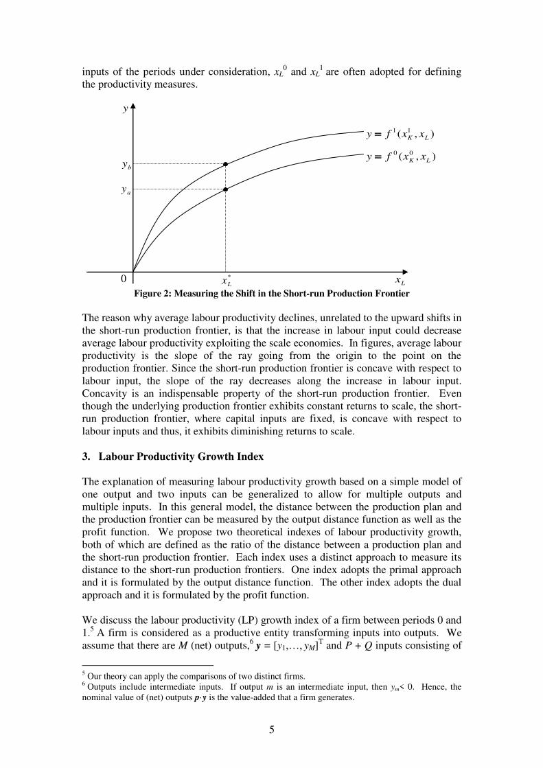
5
inputs of the periods under consideration, xL0 and xL
1 are often adopted for defining
the productivity measures.
0Lx
y
*
Lx
ay
by),( 00
LK xxfy
),( 11
LK xxfy
Figure 2: Measuring the Shift in the Short-run Production Frontier
The reason why average labour productivity declines, unrelated to the upward shifts in
the short-run production frontier, is that the increase in labour input could decrease
average labour productivity exploiting the scale economies. In figures, average labour
productivity is the slope of the ray going from the origin to the point on the
production frontier. Since the short-run production frontier is concave with respect to
labour input, the slope of the ray decreases along the increase in labour input.
Concavity is an indispensable property of the short-run production frontier. Even
though the underlying production frontier exhibits constant returns to scale, the short-
run production frontier, where capital inputs are fixed, is concave with respect to
labour inputs and thus, it exhibits diminishing returns to scale.
3. Labour Productivity Growth Index
The explanation of measuring labour productivity growth based on a simple model of
one output and two inputs can be generalized to allow for multiple outputs and
multiple inputs. In this general model, the distance between the production plan and
the production frontier can be measured by the output distance function as well as the
profit function. We propose two theoretical indexes of labour productivity growth,
both of which are defined as the ratio of the distance between a production plan and
the short-run production frontier. Each index uses a distinct approach to measure its
distance to the short-run production frontiers. One index adopts the primal approach
and it is formulated by the output distance function. The other index adopts the dual
approach and it is formulated by the profit function.
We discuss the labour productivity (LP) growth index of a firm between periods 0 and
1.5 A firm is considered as a productive entity transforming inputs into outputs. We
assume that there are M (net) outputs,6 y = [y1,…, yM]
T and P + Q inputs consisting of
5 Our theory can apply the comparisons of two distinct firms.
6 Outputs include intermediate inputs. If output m is an intermediate input, then ym< 0. Hence, the
nominal value of (net) outputs p·y is the value-added that a firm generates.
6
P types of capital inputs xK = [xK,1,…, xK,P]T and Q types of labour inputs xL = [xL,1,…,
xL,Q]T. Outputs are sold at the positive producer prices p = [p1,…, pM]
T, capital
services are purchased at the positive rental prices r = [r1,…, rP]T, and labour inputs
are purchased at the positive wage w = [w1,…, wQ]T. The period t production frontier
is presented by the period t input requirement function, F t, for t = 0 and 1:
(1) ),,(1,1, LK
t
K Fx xxy
.
It represents the minimum amount of the first capital input that a firm can use at
period t, producing the vector of output quantities y, holding fixed other capital
services xK–1 = [xK,2,…, xK,P]T and labour inputs xL.
Period t production possibility set, S
t, for t = 0 and 1 can be constructed by the period
t input requirement function. It is a feasible set of inputs and outputs attainable from
such inputs, defined as follows:
(2) }),,(:),,{( 1,1, KLK
t
LK
txFS xxyxxy .
We assume that S
t is a closed and convex set that exhibits a free disposal property.
Period t short-run production possibility set, S
t(xK
t), for t = 0 and 1 is a part of the
period t production possibility set that is conditional on the vector of capital services
xKt. It consists of a set of (y, xL) such that y can be produced by using xL, holding
constant the period t technology and capital services xKt as follows:
(3) }),,(:),{()(1,1,
t
KL
t
K
t
L
t
K
tFS xxxyxyx .
The growth of labour productivity also can be formulated in terms of the short-run
production possibility set. The expansion of the short-run production possibility set S
0(xK
0) S
1(xK
1) between periods 0 and 1 is equivalent to the improvement in labour
productivity.78
Hence, comparing the short-run production frontiers, we can recognize
the extent to which labour productivity grows. Given xK*, the short-run production
frontier for the set S
t(xK
*) is characterized by the input requirement function, F
t(y, xK,-
1*, xL) = xK,1
*.
3.1 Distance Function Approach
Caves, Christensen and Diewert (1982) introduced a theoretical index for TFP growth,
using the output distance function.9 Following them, we propose the theoretical LP
growth index using the output distance function. The period t output distance
function for t = 0 and 1 is defined as follows:
(4)
1,1, ,,:min),,( KLK
t
LK
txFD xx
yxxy
.
7 Fare, Grosskopf, Norris and Zhang (1994) also suggests that the technical progress in the sense of
TFP growth can be described by using the production possibility set such that S0 S
1.
8 The problem associated with the use of average labour productivity in Figure 2 is that average labour
productivity declines even though S
0(xK
0) S
1(xK
1).
9 In this paper, we sometimes call it the distance function for simplicity.

7
It gives the minimum amount by which an output vector y can be deflated and still
remain on the production frontier, with given input vectors xK and xL. Thus, D
t(y, xK,
xL) is considered to represent the distance between a production plan (y, xK, xL) and
the period t production frontier in the direction of outputs y. The short-run production
frontier consists of (y, xL) such as xL can produce y, holding fixed the current
technology and capital services. Hence, we can consider that D
t(y, xK
t, xL) represents
the distance between a production plan (y, xL) and the period t short-run production
frontier, in the direction of outputs y. Comparing the distances between a production
plan and the short-run production frontiers, we can measure the extent to that of short-
run production frontier shifts. We define the LP growth index between periods 0 and
1 by the ratio between the distances from a production plan to the period 0 and 1
short-run production frontiers. We define a family of the LP growth index as
follows:10
(5)),,(
),,(),,,(
11
00
10
LK
LK
LKKD
DLPG
xxy
xxyxyxx .
The distance function in the LP growth index is conditional on the reference
production plan: vectors of outputs and labour inputs, y and xL. Thus, each choice of
reference vectors y and xL might generate a different measure of the shift in
technology going from period 0 to period 1. We choose special reference vectors of
outputs and capital services to specify for the labour productivity growth index
defined by (5): a Laspeyres type measure, LPGL that chooses the period 0 reference
vectors of outputs and capital services y0 and xL
0 and a Paasche type measure, LPGP
that chooses the period 1 reference vectors of outputs and capital services y1 and xL
1.
(6)),,(
),,(),,,(
0101
0000
0010
LK
LK
LKKLD
DLPGLPG
xxy
xxyxyxx ;
(7)),,(
),,(),,,(
1111
1010
1110
LK
LK
LKKPD
DLPGLPG
xxy
xxyxyxx .
Since both measures of labour productivity growth are equally plausible, we treat the
two measures symmetrically. We define the Malmquist labour productivity growth
index as the geometric mean of the two indexes
(6) and (7);11
(8) PLM LPGLPGLPG .
10
Strictly speaking, Dt(y, xK
t, xL) is considered as the reciprocal of the distance between a production
plan (y, xL) and the period t short-run production frontier. Thus, we need to compare 1/D
t(y, xK
t, xL)
between periods t = 0 and 1 so as to capture the extent to that the short-run production frontier shifts.
Thus, the shift between periods t = 0 and 1 is defined as D
0(y, xK
0, xL)/D
1(y, xK
1, xL) rather than D
1(y,
xK1, xL)/D
0(y, xK
0, xL).
11 Since the firm‟s profit maximization is assumed, it is possible to adopt a different formulation for the
Malmquist LP growth index: LPGM1 = (D
0(y
1, xK
0, xL
1 )/D
0(y
0, xK
0, xL
0 ))
1/2(D
1(y
1, xK
1, xL
1 )/ D
1(y
0, xK
1,
xL0 ))
1/2. This formulation is closer to the original Malmquist productivity (TFP growth) index.

8
0
A
B
0
Lx1
Lx Lx
y
C
D
cyy 0
dy
ey
fyy 1
),( 00
LK xxfy
),( 11
LK xxfy
Figure 3: The Malmquist and Diewert-Morrison LP growth indexes
In the case of one output and two inputs, it is easy to give a graphical interpretation of
the Malmquist LP growth index. It coincides with the following formula, as shown in
Figure 3.
(9)
e
f
c
d
My
y
y
yLPG .
Given a quantity of labour input, the ratio of the output attainable from such a labour
input at period 1 to the output attainable at period 0 represents the extent to which the
short-run production function expands. LPGM is interpreted as the geometric mean of
the ratios conditional on the period 0 labour input and the period 1 labour input.
The Malmquist LP growth index is a theoretical index in the sense that it is defined as
the ratio of the distance functions. At this point, it is not clear how we will obtain
empirical estimates for the theoretical labour productivity growth indexes defined by
(8). One obvious way is econometric approach. In this approach, we assumes a
functional form for the distance function D
t(y, xK, xL), collect data on prices and
quantities of outputs and inputs for a number of years, add error terms and use
econometric techniques to estimate the unknown parameters in the assumed
functional form. However, econometric techniques are generally not completely
straightforward. Different econometricians will make different stochastic
specifications and will choose different functional forms.12
Moreover, as the number
of outputs and inputs grows, it will be impossible to estimate a flexible functional
form. Thus in the following section, we will suggest methods for estimating LP
growth index (8) that are based on exact index number techniques.
Caves, Christensen and Diewert (1982) have shown that the first-order derivatives of
the distance function Dt with respect to quantities at the period t actual production
plan are computable from observable prices and quantities of inputs and outputs.
12
“The estimation of GDP functions such as (19) can be controversial, however, since it raises issues
such as estimation technique and stochastic specification. ... We therefore prefer to opt for a more
straightforward index number approach.” Kohli (2004).
9
They used these relationships to show that the Malmquist productivity index coincides
with the Törnqvist productivity index, which is a formula of prices and quantities.13
We use the same relationships to show that the Malmquist LP growth index coincides
with a formula of observable prices and quantities. Although all these relationships
have been already derived by Caves, Christensen and Diewert (1982), we outline how
to compute the first-order derivatives of the distance functions below for
completeness of discussion. The implicit function theorem is applied to the input
requirement function F
t(y/δ, xK,–1, xL) = xK,1 to solve for δ = D
t(y, xK, xL) around (y
t,
xKt, xL
t).
14 In this case, D
t(y, xK, xL) is differentiable around the point (y
t, xK
t, xL
t). Its
derivatives are represented by the derivatives of F
t(y, xK, xL). We have the following
equations for periods t = 0 and 1:
(10) ),,(),,(
1),,( t
L
t
K
tt
t
L
t
K
ttt
t
L
t
K
ttF
FD xxy
xxyyxxy y
y
y
;
(11)
t
L
t
K
ttt
L
t
K
ttt
t
L
t
K
tt
FFD
K
K xxyxxyyxxy
xy
x ,,(
1
),,(
1),,(
1,1, 1,
;
(12) ),,(),,(
1),,( t
L
t
K
tt
t
L
t
K
ttt
t
L
t
K
ttF
FD
LLxxy
xxyyxxy x
y
x
.
We assume that (yt, xK,
t xL
t) >> 0N+P+Q is a solution to the following period t profit
maximization problem for t = 0 and 1:
(13) }),,(max{ 1,11,1 L
t
K
t
LK
tttFr xwxrxxyyp .
The period t profit maximization problem yields the following first order conditions
for t = 0 and 1:
(14) ),,( 1,1
t
L
t
K
ttttFr xxyp y ;
(15) ),,( 1,11 1,
t
L
t
K
tsttFr
Kxxyr x
;
(16) ),,( 1,1
t
L
t
K
tsttFr
Lxxyw x .
By substituting (14), (15) and (16) into (10), (11) and (12), we obtain the following
equations for t = 0 and 1:
(17)tttt
L
t
L
ttD yppxxyy /),,( ;
(18) tttt
L
t
K
tttttt
L
t
K
tt
FrD
K
Kypr
xxyypxxy
xx
/),,(
1)]/([),,(
1,1
1,
;
(19) ypwxxyx ttt
L
t
L
ttD
L/),,( .
13
The Malmquist productivity index is TFP growth index. 14
We assume the following three conditions are satisfied for t = 0 and 1: 1) F
t is differentiable at the
point (yt, xK
t, xL
t),: 2) y
t >> 0M and 3) y
t∙ y F
t(y
t, xK
t, xL
t) > 0.
10
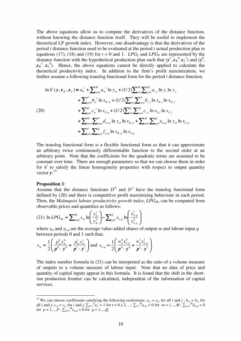
The above equations allow us to compute the derivatives of the distance function,
without knowing the distance function itself. They will be useful to implement the
theoretical LP growth index. However, one disadvantage is that the derivatives of the
period t distance function need to be evaluated at the period t actual production plan in
equations (17), (18) and (19) for t = 0 and 1. LPGL and LPGP are represented by the
distance function with the hypothetical production plan such that (y1, xK
0, xL
1) and (y
0,
xK1, xL
0). Hence, the above equations cannot be directly applied to calculate the
theoretical productivity index. In addition to the firm‟s profit maximization, we
further assume a following translog functional form for the period t distance function.
(20)
P
p
Q
q qLpKqp
M
m
Q
q qLmqm
M
m
P
p pKmpm
Q
i
Q
j jLiLji
Q
q qL
t
q
P
i
P
j jKiKji
P
p pK
t
p
M
i
M
j jiji
M
m m
t
m
t
LK
t
xxf
xyexyd
xxcxc
xxbxb
yyayaah
1 1 ,,,
1 1 ,,1 1 ,,
1 1 ,,,1 ,
1 1 ,,,1 ,
1 1 ,10
lnln
lnlnlnln
lnln)2/1(ln
lnln)2/1(ln
lnln)2/1(ln),,(ln xxy
The translog functional form is a flexible functional form so that it can approximate
an arbitrary twice continuously differentiable function to the second order at an
arbitrary point. Note that the coefficients for the quadratic terms are assumed to be
constant over time. There are enough parameters so that we can choose them in order
for ht to satisfy the linear homogeneity properties with respect to output quantity
vector y:15
Proposition 1:
Assume that the distance functions D
0 and D
1 have the translog functional form
defined by (20) and there is competitive profit maximizing behaviour in each period.
Then, the Malmquist labour productivity growth index, LPGM, can be computed from
observable prices and quantities as follows:
(21)
Q
qqL
qL
qL
M
mm
m
mMx
xs
y
ysLPG
1 0
,
1
,
,1 0
1
lnlnln
where sm and sL,q are the average value-added shares of output m and labour input q
between periods 0 and 1 such that;
11
11
00
00
2
1
ypyp
mmmm
m
ypyps and
11
1
,
1
00
0
,
0
,2
1
ypyp
qLqqLq
qL
xwxws .
The index number formula in (21) can be interpreted as the ratio of a volume measure
of outputs to a volume measure of labour input. Note that no data of price and
quantity of capital inputs appear in this formula. It is found that the shift in the short-
run production frontier can be calculated, independent of the information of capital
services.
15
We can choose coefficients satisfying the following restrictions; ai,j = aj,i for all i and j ; bi,j = bj,i for
all i and j; ci,j = cj,i for i and j; ∑n=1Nan
t = 1 for t = 0,1,2, ...; ∑i=1
Mai,m = 0 for m = 1,...,M ; ∑m=1
Mdm,p = 0
for p = 1,...,P ; ∑m=1M
em,q = 0 for q = 1,...,Q.
11
3.2 Profit Function Approach
The research on productivity measurement based on the restricted profit function goes
back to Diewert and Morrison (1986).16
Given prices of outputs and quantities of
primary inputs, the change in the profit can be attributed to productivity changes.
Diewert and Morrison (1986) define the theoretical TFP growth index as a ratio of the
profit function between two periods, given output prices and primary input quantities.
In the end, it is shown that their theoretical TFP growth index coincides with the
implicit Törnqvist productivity index.17
Given an output price vector p and input quantity vectors xK and xL, we define the
period t restricted profit function, g
t(p, xK, xL) for t = 0 and 1, as follows:
(22) }),,(:{max),,( 1,1,, KLK
t
LK
txFg
L xxyypxxp xy .
Thus, the profit of the firm depends on the period t technology and the output price
vector p and input quantity vectors xK and xL.
If pt is the period t output price vector and xK
t and xL
t are the vectors of factor inputs
used during period t, and if the profit function is differentiable with respect to the
components of p and w at the point (pt, wL
t, xK
t), then the period t vector of the firm‟s
net outputs yt and capital inputs xL
t will be equal to the vector of first order partial
derivatives of g
t(p
t, wL
t, xK
t) with respect to the components of p and w. We will have
the following equation for periods t = 0 and 1:18
(23) ),,( t
L
t
K
tttg xxpy P .
If the restricted profit function is differentiable with respect to the quantities of capital
inputs xK at the point (pt, wL
t, xK
t), then the period t vector of input prices r
t will be
equal to the vector of first order partial derivatives of g
t(p
t, wL
t, xK
t) with respect to the
components of the quantities of capital services xK. We will have the following
equations for periods t = 0 and 1:19
(24) ),,( t
L
t
K
tttg
Kxxpr x ;
(25) ),,( t
L
t
K
tttg
Lxxpw x .
The above equations allow us to compute the derivatives of the restricted profit
function without knowing the profit function itself. They will be useful to implement
the theoretical LP growth index.
We maintain the idea that the LP growth index should reflect the shift in the short-run
production frontier. In the dual representation, the shift in the restricted profit
function reflects the shift in the short-run production frontier. Thus, we define the LP
16
In this paper, we sometimes call it the profit function for simplicity. 17
It equals the implicit Törnqvist output quantity divided by the Törnqvist input quantity index. 18
These relationships are due to Hotelling (1932). 19
These relationships are due to Samuelson (1953) and Diewert (1974).
12
growth index by the growth rate of the restricted profit function caused by
technological progress and the increase in capital services. We define a family of the
labour productivity growth index as follows:
(26)),,(
),,(),,,(
00
1101
LK
LK
LKKg
gLPG
xxp
xxpxpxx .
The restricted profit function in the productivity index is conditional on the output
price vector p and the vector of labour input xL. Thus, each choice of reference output
price vector p and reference vector of labour input xL will generate a possibly different
measure of the shift in technology from period 0 to period 1. We choose special
reference output price vector p and special reference vector of labour input xL for the
labour productivity growth index defined by (26): a Laspeyres type measure, LPGL
that chooses the period 0 reference output price vector p0 and the period 0 reference
vector of labour input xL0 and a Paasche type measure, LPGP that chooses the period
1 reference output price vector p1 and the period 1 reference vector of labour input
xL1:
(27)),,(
),,(),,,(
0000
0101
0001
LK
LK
LKKLg
gLPGLPG
xxp
xxpxpxx ;
(28)),,(
),,(),,,(
1010
1111
1101
LK
LK
LKKPg
gLPGLPG
xxp
xxpxpxx .
Since both measures of technical progress are equally valid, it is natural to average
them to obtain an overall measure of labour productivity growth. If we want to treat
the two measures in a symmetric manner and we want the measure to satisfy the time
reversal property from the difference approach to index number theory (so that the
estimate going backwards is equal to the negative of the estimate going forwards),
then the arithmetic mean will be the best simple average to take. Thus, we define the
Diewert-Morrison labour productivity growth index (hereafter, Diewert-Morrison LP
growth index) by the arithmetic mean of (27) and (28) as follows:
(29) PLDM LPGLPGLPG .
The Diewert-Morrison LP growth index can be also illustrated graphically in Figure 3.
It coincides with the Malmquist LP growth index in this simple model of one output
and two inputs.
(30)
e
f
c
d
e
f
c
d
DMy
y
y
y
yp
yp
yp
ypLPG
1
1
0
0
.
The Diewert-Morrison LP growth index is a theoretical index in the sense that it is
defined by the restricted profit function. LPGL and LPGP are represented by the
restricted profit function with the hypothetical production plan such that (p1, xK
0, xL
1)
and (p0, xK
1, xL
0). Hence, the equations (23)(24)(25) cannot be directly applied to
calculate the theoretical productivity index. In addition to the firm‟s profit
13
maximization, we further assume a following translog functional form for the period t
restricted profit function.
(31)
P
p
Q
q qLpKqp
M
m
Q
q qLmqm
M
m
P
p pKmpm
Q
i
Q
j jLiLji
Q
q qL
t
q
P
i
P
j jKiKji
P
p pK
t
p
M
i
M
j jiji
M
m m
t
m
t
LK
t
xxf
xpexpd
xxcxc
xxbxb
ppapaaH
1 1 ,,,
1 1 ,,1 1 ,,
1 1 ,,,1 ,
1 1 ,,,1 ,
1 1 ,10
lnln
lnlnlnln
lnln)2/1(ln
lnln)2/1(ln
lnln)2/1(ln),,(ln xxp
The translog functional form is a flexible functional form so that it can approximate
an arbitrary twice continuously differentiable function to the second order at an
arbitrary point. Note that the coefficients for the quadratic terms are assumed to be
constant over time. There are enough parameters so that we can choose them in order
for Ht to satisfy the linear homogeneity properties with respect to output price vector
p:20
Proposition 2:
Assume that the profit functions g0 and g
1 have the translog functional form defined
by (31).21
Then, the Diewert-Morrison labour productivity growth index, LPGDM, can
be computed from observable prices and quantities as follows:
(32)
Q
qqL
qL
qL
M
mm
m
mDMx
xs
p
psLPG
1 0
,
1
,
,1 0
1
00
11
lnlnlnlnyp
yp
where sm and sL,q are the average value-added shares of output m and labour input q
between periods 0 and 1 such that;
11
11
00
00
2
1
ypyp
mmmm
m
ypyps and
11
1
,
1
00
0
,
0
, 2
1
ypyp
qLqqLq
qL
xwxws .
It turns out that both labour productivity growth indexes based on the distance
function and the profit function coincide with the almost identical index number
formula. Both are interpreted as the ratio of a quantity index of output to a quantity
index of labour input. For labour inputs, both use the same quantity index for labour
inputs. On the other hand, there is a difference in the output quantity index. While
the Malmquist labour productivity index uses the Törnqvist quantity index, the
Diewert-Morrison labour productivity index uses the implicit Törnqvist quantity index.
However, the Törnqvist and the implicit Törnqvist quantity indexes are superlative
indexes, which are immune from the substitution bias associated with the Laspeyres
and Paasche indexes. Since it is known that the difference between superlative
20
We can choose coefficients satisfying the following restrictions; ai,j = aj,i for all i and j ; bi,j = bj,i for
all i and j; ci,j = cj,i for i and j; ∑n=1Nan
t = 1 for t = 0,1,2, ...; ∑i=1
Mai,m = 0 for m = 1,...,M ; ∑m=1
Mdm,p = 0
for p = 1,...,P ; ∑m=1M
em,q = 0 for q = 1,...,Q. 21
For the case of the restricted profit function, the linear homogeneity with respect to output price
vector p is satisfied.

14
indexes is minor (Diewert, 1978), the difference between the Malmquist and Diewert-
Morrison LP growth indexes is negligible.22
3.3 Comparison with Average Labour Productivity Growth
We compare two new indexes of labour productivity growth, LPGM and LPGDM, with
the standard productivity measure of average labour productivity. We treat the
growth in average labour productivity as an index of labour productivity growth and
call it the average labour productivity (LP) growth index, which is denoted by ALPG.
By definition, the average LP growth index equals the ratio of the growth rate of
output quantity to the growth rate of labour input quantity. Given multiple outputs
and labour inputs, it is necessary to use the quantity index to aggregate the growth of
multiple outputs and labour inputs. We consider two types of the average LP growth
indexes, denoted by ALPGT and ALPGImT. Both apply the Törnqvist quantity index to
aggregating the growth rates of labour inputs. However, for aggregating changes of
outputs, one index, ALPGT, uses the Törnqvist quantity index, and the other index,
ALPGImT, uses the implicit Törnqvist quantity index.
(33)
Q
qqL
qLqL
M
mm
m
mTx
xs
y
ysALPG
1 0
,
1
,,
1 0
1
lnlnln ;
(34)
Q
qqL
qLqL
M
mm
m
mImTx
xs
p
psALPG
1 0
,
1
,,
1 0
1
00
11
lnlnlnlnyp
yp;
where sm is the average value-added shares of output m and qLs , is the average labour-
compensation share of labour input q between periods 0 and 1 such that;
11
11
00
00
2
1
ypyp
mmmm
m
ypyps and
11
1
,
1
00
0
,
0
,
2
1
L
qLq
L
qLqqL
xwxws
xwxw.
While ALPGT corresponds to the Malmquist LP growth index, LPGM, using the
Törnqvist quantity index for aggregating the quantity growth of outputs, the ALPGImT
corresponds to the Diewert-Morrison LP growth index, LPGDM, using the implicit
Törnqvist quantity index for aggregating the quantity growth of outputs. As we
discussed for the difference between Malmquist and Diewert-Morrison LP growth
indexes, the difference between two average LP growth indexes, ALPGT and ALPGImT
is negligible.
(35)
Q
qqL
qL
L
qLqK
L
qLqK
TDMTM
x
xxwxw
ALPGLPGALPGLPG
1 0
,
1
,
11
1
,
1
11
11
00
0
,
0
00
00
Im
lnxwyp
xr
xwyp
xr
The difference between the average LP growth indexes (ALPGT and ALPGImT) and the
new LP growth indexes (Malmquist and Diewert-Morrison LP growth indexes, LPGM
and LPGDM) comes from the weight attached to the growth of labour inputs. While
ALPGT and ALPGImT weight different types of labour inputs with their shares in total
labour compensation, LPGM and LPGDM weight different types of labour inputs with
22
The Fisher quantity index is another superlative index. See Diewert (1976).

15
their shares in value-added. This is reflected in the differences between LPGM and
ALPGT or between LPGM and ALPGT, as shown in equation (35). Since ALPGT and
ALPGImT gives more weight to each type of labour input than LPGM and LPGDM,
ALPGT and ALPGImT are larger than LPGM and LPGDM, as long as the quantities of
labour inputs grow. The larger capital share, the larger the difference between them
becomes.
As we pointed out in the previous section, the difference between the average LP
growth index and the Malmquist LP growth index is attributed to the effect of scale
economies. Equation (35) shows when its effect is enhanced. Under the concave
production frontier, the more labour input increases, the more average labour
productivity declines. It is possible to interpret that the larger share of capital inputs
indicates the flatter slope of the short-run production frontier.23
Along the short-run
production frontier that has a flatter slope, the impact of the change in labour input
will be strengthened.
4. Aggregation over Industries
We discuss a good aggregation property which the Malmquist and Diewert-Morrison
LP growth indexes satisfy. Aggregation of the LP growth indexes is necessary for
many cases. The aggregation property of the LP growth indexes, which we will
discuss below, holds for any type of aggregation problem. However, we restrict our
discussion to the aggregation over industries in particular for simplicity.
We have followed discrete time approach to the productivity measurement up to the
previous section. In this approach, the price and quantity data are defined only for
integer values of t, which denote discrete unit time periods. There is another approach
called the Divisia approach. In this approach, the price and quantity data are defined
as functions of continuous time.24
Thus, the logarithm of the ratio of some variable
between period 0 and 1 is replaced by the time derivative of that variable. The
average share of revenue from each output in total value-added (1/2)(pm0ym
0/p
0·y
0 +
pm1ym
1/p
1·y
1) is now identically specified by pmym/p·y. We apply the Divisia approach
to the two LP growth indexes, LPGM and LPGDM, and discuss their aggregation
properties.25
There are J types of industries. For each industry, yj is output vector for an industry j,
xKj and xL
j are input quantity vectors of capital services and labour inputs for an
industry j such as yj ≡ [y1
j,…, yMj]
T, xK
j ≡ [xK,1
j,…, xK,Pj]
T and xL
j ≡ [xL,1
j,…, xL,Qj]
T
where ymj is quantity of output m produced by an industry j, xK,p
j and xL,q
j are
quantities of capital service p and labour input q utilized by an industry j. The
quantities of output m produced by each industry sum up to the aggregate quantity of
output m, ym and similarly, the quantities of capital service p used by each industry
sum up to the aggregate quantity of capital service p and the quantity of labour input q
23
If we assume a Cobb-Douglas production function, the slope of the short-run production function is a
function of the share of capital income to total value added. The large share of capital income makes
the slope flatter, holding fixed capital services and labour inputs. 24
The Divisia approach is coined by Diewert and Nakamura (2007). See Hulten (1973) and Balk
(2000) for detailed in Divisia approach. 25
In the Divisia approach, since there is no difference between the Törnqvist quantity index and the
implicit Törnqvist quantity index, LPGM and LPGDM are the same. Thus, although we only discuss
LPGM, the aggregation property we discuss here is also shared by LPGDM.
16
used by each industry sum up to the aggregate quantity of labour input q such that ym
= ∑j=1Jym
j, xK,p = ∑j=1
JxK,p
j and xL,q
j = ∑j=1
JxL,q
j. We assume that the prices of the same
output and the same input are constant across industries. Applying equation (34), we
can calculate the economy-wide Malmquist LP growth index LPGM,T as well as the
industry j Malmquist LP growth index LPGM,j as follows:
(36)
J
j j
qK
j
qKQ
q J
j
jj
j
qL
j
q
J
j j
m
j
mM
m J
j
jj
j
m
j
m
TM
x
xxw
y
yypLPG
1,
,
1
1
,
1 1
1
,
1
1
yp
yp
(37)
j
qK
j
qKQ
q
j
qL
j
q
j
m
j
mM
m
j
m
j
m
jMx
xxw
y
yypLPG
,
,
1
,
1, 11
ypyp.
From equations (36) and (37), we can derive the following relationship between the
economy-wide LP growth and the industry LP growth indexes:
(38)
J
j jMJ
j
jj
jj
TM LPGLPG1 ,
1
,
yp
yp.
Equation shows that the economy-wide LP growth index is the average of the industry
LP growth index, weighted by the industry‟s value-added share. Thus, the use of
these two LP growth indexes, LPGM or LPGDM, enables us to precisely identify the
contribution of each industry to the economy-wide LP growth. It enables us to
investigate the industry origins of the economy-wide LP growth.
5. An Application to the U.S. Industry Data
We apply the labour productivity growth indexes to investigate the industry
productivity performance of the U.S. for the period 1970-2005. The U.S. industry
data is taken from the comprehensive industry dataset called the EU KLEMS Growth
and Productivity Accounts.26
Industry accounts that we used consist of gross outputs
and intermediate inputs at current and constant prices, and hours worked of
employment by 30 industries.27
These industry data are organized according to the
System of Industry Classification (SIC) adopted by the U.S. official statistics.
26
Data are downloaded from the EU KLEMS website (http://www.euklems.net/). The detailed
explanation about this comprehensive international database is found in O‟Mahony and Timmer (2009).
The U.S. industry data of EU KLEMS is constructed by Dale Jorgenson and his research group. See
Jorgenson, Ho and Stiroh (2008). 27
For each industry, there exist one type of gross output and one type of intermediate input. Their
deflator varies across industries. Labour input is hours worked by total employment. Total
employment in each industry includes employees and the self-employed engaged in the production of
the industry.

17
Figure 4 compares the economy-wide average and Malmquist LP growth indexes for
the entire sample period 1970-2005. Since the Diewert-Morrison LP growth index is
almost identical to the Malmquist LP growth index, we exclude the former index from
the figure.28
Equation (35) shows that the difference between the average LP growth
index and the Malmquist LP growth index, which can be attributed to the effect of
scale economies, depends on the growth rate of hours worked and the nominal share
of capital input in total value added. Total hours worked for the U.S. was stagnated in
some years but it was on the overall upward trend.29
The widening gap between the
average LP growth index and the Malmquist LP growth index reflects this increasing
trend of hours worked. The economy-wide capital share also increased over years
from 33.0 per cent in 1970 to 39.7 per cent in 2005.
Total industries (1970=1)
1.0
1.2
1.4
1.6
1.8
2.0
2.2
1970 1974 1978 1982 1986 1990 1994 1998 2002
Average labour productivity
Malmquist labour productivity
Figure 4: Economy-wide Average and Malmquist LP growth indexes, 1970-2005
We investigate the industry origins of the economy-wide labour productivity growth.
The entire sample period 1970-2005 can be usefully divided into three periods: 1970-
1995, 1995-2000 and 2000-2005.30
Industry productivity performance has been
stagnated since the early 1970s. 1995 is the watershed year when the productivity of
the U.S. industries revived again. Productivity growth even accelerated in 2000s.
Table 1: Annual Average: Average and Malmquist LP Growth Indexes
Average Malmquist Average Malmquist Average Malmquist Average Malmquist
Total industries 1.5% 2.0% 1.2% 1.8% 1.8% 2.7% 2.8% 2.7%
Electrical and optical equipment 11.0% 10.9% 9.2% 9.3% 20.0% 20.3% 11.4% 9.8%
Other manufacturing 2.4% 2.2% 1.8% 1.8% 3.2% 3.2% 4.7% 3.2%
Other production -0.5% 0.1% -0.5% 0.0% -0.2% 1.2% -1.1% -0.6%
Post and communication 5.1% 5.4% 4.8% 5.1% -0.3% 2.5% 12.1% 9.5%
Other market services 1.7% 2.3% 1.4% 2.0% 1.7% 2.6% 3.1% 3.1%
Distribution 2.7% 3.1% 2.5% 2.8% 2.5% 3.1% 4.4% 4.2%
Finance and business, except real estate 0.6% 1.7% 0.2% 1.3% 0.8% 2.4% 2.8% 2.7%
Personal services 0.1% 0.5% -0.3% 0.2% -0.1% 0.4% 1.8% 2.0%
Non-market services 0.8% 1.6% 0.7% 1.6% 0.7% 1.3% 1.5% 2.1%
1995-2000 2000-20051970-2005 1970-1995
28
From the same reason, we did not report the Diewert-Morrison LP growth index in any figures and
tables, hereafter. 29
Hours worked decreased in 1971, 1975, 1980, 1982, 1991 and 2000-03. 30
It is known that the stagnation of the U.S. economy started since 1973. Since the dataset is available
since 1970 and the period 1970-1973 is small enough to know the overall trend, we deal with the
period 1970-1995.

18
The 30 industries are classified into 6 representative industries: 1) Electrical and
other equipment, 2) Other manufacturing, 3) Other production, 4) Post and
communication, 5) Other market services, and 6) Non-market services. Electrical and
other equipment is manufacturing and post and communication showed is service
sector. However, since they show very different performance within the
manufacturing and service sectors, they are isolated from other manufacturing and
other market services and non-market services. Table 1 compares the annual average
growth rates of labour productivity based on the average and Malmquist LP growth
indexes.
There is a hypothesis so called “Baumol‟s disease” stating that labour productivity
growth in the service sector is likely to be stagnated and lower than that of goods
producing industries, especially the manufacturing sector. It has been widely
advocated by Triplett and Bosworth (2004), (2006) and Bosworth and Triplett (2007).
Except for distribution in other market services, the average LP growth index among
the service sectors is lower than other manufacturing, as shown in Table 1. On
average over the entire sample period 1970-2005, the average growth rates of other
market sectors and non-market services are 1.7 per cent and 0.8 per cent, which are
smaller than that of other manufacturing, which is 2.4 per cent. However, if we
compare these industries by the Malmquist LP growth index, the average growth rates
of other market sectors and non-market services are 2.3 per cent and 1.6 per cent,
while that of other manufacturing is 2.2 per cent. The difference in the growth of
labour productivity between the service sectors and other manufacturing based on the
average LP index becomes much smaller under the comparison based on the
Malmquist LP growth index. This underestimation of the industry labour
productivities by the average LP growth index is even more severe during the low
productivity growth period 1970-1995. Two indexes are almost the same for
manufacturing. However, moving from the average LP growth index to the
Malmquist LP growth index, the labour productivity growth in the service sectors
becomes much larger. For the period 1970-1995, the average growth rate of the
Malmquist LP growth index of other market services is 2.0 per cent, even higher than
that of other manufacturing 1.8 per cent. The average growth rate for non-market
services is 1.6 per cent, close to that of other manufacturing. The productivity
resurgence of service sectors since 1995 made Triplett and Bosworth (2007) state that
Baumol‟s disease has been cured. Under the comparison of industry labour
productivity based on the Malmquist LP growth index, we conclude that although
Baumol‟s disease exists before 1995, this disease has not been as serious as it
appeared.
Table 2: Growth Rate of Hours Worked and Share of Capital Input in Value Added
1970-2005 1970-1995 1995-2000 2000-2005
Total industries 1.4% 1.6% 2.2% -0.3% 36.4%
Electrical and optical equipment -0.2% 0.6% 0.8% -5.4% 25.4%
Other manufacturing -0.7% -0.2% -0.1% -4.2% 31.4%
Other production 1.5% 1.2% 3.5% 1.0% 41.4%
Post and communication 0.5% 0.6% 4.9% -4.3% 54.4%
Other market services 2.2% 2.5% 3.2% -0.1% 25.7%
Distribution 1.3% 1.6% 2.0% -0.7% 25.8%
Finance and business, except real estate 3.6% 4.1% 5.1% -0.1% 29.2%
Personal services 2.4% 2.6% 2.9% 0.7% 17.1%
Non-market services 1.7% 1.8% 1.3% 1.3% 47.8%
Growth of Hours Worked Share of Capital
1970-2005

19
The difference between two LP growth indexes comes from the large share of capital
input and the high growth rate of hours worked. Table 2 shows that the difference
between two indexes is significant for the sectors whose hours worked steadily
increased over the period. The growth rate of hours worked is much higher in the
service sectors than in the manufacturing sector. This flow of labour inputs from the
manufacturing sectors to the service sectors can explain the pessimistic view on the
service sector, expressed by Baumol‟s disease.
Figure 5 shows the long term trend of the average and Malmquist LP growth indexes
for the period 1970-2005. Overall trend are quite similar in two indexes. However,
the movements of two indexes are different in shorter period of time by reflecting the
drastic changes in hours worked in the service sector.
Figure 5: Average and Malmquist LP Growth Indexes by Sector, 1970-2005
Other manufacturing (1970=1)
1.0
1.2
1.4
1.6
1.8
2.0
2.2
2.4
2.6
1970 1974 1978 1982 1986 1990 1994 1998 2002
Average labour productivity
Malmquist labour productivity
Other production (1970=1)
0.7
0.8
0.9
1.0
1.1
1970 1974 1978 1982 1986 1990 1994 1998 2002
Average labour productivity
Malmquist labour productivity
Other market services (1970=1)
1.0
1.2
1.4
1.6
1.8
2.0
2.2
2.4
1970 1974 1978 1982 1986 1990 1994 1998 2002
Average labour productivity
Malmquist labour productivity
Non-market services (1970=1)
1.0
1.1
1.2
1.3
1.4
1.5
1.6
1.7
1.8
1.9
1970 1974 1978 1982 1986 1990 1994 1998 2002
Average labour productivity
Malmquist labour productivity
Electrical and optical equipment (1970=1)
1
6
11
16
21
26
31
36
41
46
51
1970 1974 1978 1982 1986 1990 1994 1998 2002
Average labour productivity
Malmquist labour productivity
Post and communication (1970=1)
1.0
2.0
3.0
4.0
5.0
6.0
7.0
1970 1974 1978 1982 1986 1990 1994 1998 2002
Average labour productivity
Malmquist labour productivity

20
We examine the productivity performance of the service sector in more detailed.
Table 3 compares labour productivity of 13 sub-industries in the service sector. Table
4 shows the annual average growth rate of hours worked and the share of capital input
in nominal industry value added for each sub-industry. The difference between the
average LP growth index and the Malmquist LP growth index diverges especially for
renting equipment and other business activities, and real estate activities for the
period 1970-2005. However, its reason differs between two sub-industries. Hours
worked for renting equipment and other business services grew at average annual rate
of 4.7 per cent. This is far above the average growth rate of other service industries,
widening the gap between two LP growth indexes in renting equipment and other
business activities. The average growth rate of hours worked for real estate activities
is 2.6 per cent. There are other sub-industries such as hotels and restaurants and
health and social work whose hours worked grew much faster than real estate
activities. The reason why the difference between two LP growth indexes
significantly widens only for real estate activities is the large share of capital input in
the value added for this sub-industry. It is almost 90 per cent and is incomparably
high within all the industries. The impact of the growth in hours worked of real estate
activities is strengthened with the larger capital share.
Table 3: Annual Average: Average and Malmquist LP Growth Indexes in Service Sector
Average Malmquist Average Malmquist Average Malmquist Average Malmquist
Other market services
Distribution
Sale, maintenance and repair of motor vehicles and motorcycles 3.7% 4.3% 2.8% 3.4% 5.0% 6.4% 6.4% 6.2%
Wholesale trade and commission trade 3.8% 4.2% 4.3% 4.7% 2.6% 3.0% 3.0% 2.7%
Retail trade 2.0% 2.2% 0.8% 1.1% 3.4% 3.7% 6.3% 6.2%
Transport and storage 1.7% 2.1% 1.6% 2.0% 0.1% 0.9% 3.9% 3.7%
Finance and business services
Financial intermediation 2.8% 3.6% 2.6% 3.4% 4.5% 5.8% 2.1% 2.2%
Renting of equipment and other business activities -0.8% 0.2% -1.6% -0.4% -1.0% 0.1% 3.1% 3.1%
Personal services
Hotels and restaurants -1.5% -0.9% -2.6% -1.9% -0.6% 0.0% 3.0% 2.9%
Other community, social and personal services 1.0% 1.4% 1.3% 1.7% -0.3% 0.3% 0.9% 1.2%
Private households with employed persons 0.6% 0.6% 0.7% 0.7% 0.0% 0.0% 0.2% 0.2%
Non-market services
Public administration and defence 1.0% 1.1% 1.2% 1.3% 1.0% 0.9% 0.4% 0.5%
Education 0.2% 0.8% 0.3% 0.9% -0.2% 0.4% 0.5% 0.8%
Health and social work -0.3% 0.3% -1.0% -0.4% 0.8% 1.0% 2.5% 2.8%
Real estate activities 0.9% 3.3% 0.7% 3.3% -0.1% 2.4% 2.8% 4.0%
1970-2005 1970-1995 1995-2000 2000-2005
Table 4: Growth Rate of Hours Worked and Share of Capital Input in Value Added in
Service Sector
1970-2005 1970-1995 1995-2000 2000-2005
Other market services
Distribution
Sale, maintenance and repair of motor vehicles and motorcycles 1.2% 1.1% 3.1% -0.4% 43.8%
Wholesale trade and commission trade 1.3% 1.7% 1.7% -1.2% 26.5%
Retail trade 1.4% 1.6% 1.7% -0.3% 15.2%
Transport and storage 1.3% 1.5% 2.5% -1.0% 29.1%
Finance and business services
Financial intermediation 2.0% 2.3% 2.6% 0.3% 41.8%
Renting of equipment and other business activities 4.7% 5.4% 6.2% -0.3% 20.2%
Personal services
Hotels and restaurants 3.0% 3.8% 2.4% -0.3% 21.2%
Other community, social and personal services 2.5% 2.4% 3.8% 1.5% 15.3%
Private households with employed persons -0.9% -1.5% -1.8% 2.7% 0.0%
Non-market services
Public administration and defence 0.2% 0.2% -0.2% 0.4% 33.3%
Education 2.2% 2.2% 2.9% 1.5% 24.0%
Health and social work 3.3% 3.9% 1.4% 2.0% 16.7%
Real estate activities 2.6% 2.8% 2.8% 1.4% 89.8%
Growth of Hours Worked Share of Capital
1970-2005

21
6. Conclusion
Total factor productivity growth has been theoretically defined as the shift in the
production frontier caused by technological progress. We examine the same
reasoning applied to the measurement of labour productivity growth. We start from
the viewpoint that the labour productivity growth index should capture the shift in the
short-run production frontier caused by technological progress and the change in
capital services. We propose the Malmquist and Diewert-Morrison labour
productivity growth indexes, which capture the shift, by using the distance function as
well as the profit function. Following the index number techniques initiated by Caves,
Christensen and Diewert (1982) and Diewert and Morrison (1987), we show that these
two indexes equal the index number formulae consisting of observable prices and
quantities. These indexes also have a good aggregation property that the standard
average labour productivity growth index does not satisfy. In the end, we apply the
average and Malmquist labour productivity growth indexes to the industry data of the
U.S. for the period 1970-2005. It is well known that the low labour productivity
growth of the service sector drags down the growth rate of labour productivity for the
entire U.S. economy. However, we found that the difference in the Malmquist labour
productivity growth index between the service sector and other sectors is much
smaller than the difference in the average labour productivity between them. The
underestimation of the labour productivity growth in the service sector by average
labour productivity is even more serious in the low productivity era before 1995. The
difference between the average and the Malmquist labour productivity growth indexes
can be attributed to the effect of scale economies, which grows throughout the change
in labour inputs. The flow of employment from the manufacturing sector to the
service sector accounts for the underestimation of productivity performance of the
service sector during the low productivity era before 1995.

22
References
Balk, B.M. (2000), “Divisia Price and Quantity Indexes: 75 Years After”, Department
of Statistical Methods, Statistics Netherlands
Bosworth, B.P. and J.E. Triplett (2007), “The Early 21st Century U.S. Productivity
Expansion is Still in Services”, International Productivity Monitor 14, 3-19.
Caves, D.W., L. Christensen and W.E. Diewert (1982), “The Economic Theory of
Index Numbers and the Measurement of Input, Output, and Productivity”, Econometrica 50, 1393-1414.
Chambers, R.G. (1988), Applied Production Analysis: A Dual Approach, New York:
Cambridge University Press.
Diewert, W.E. (1974), “Applications of Duality Theory,”, in M.D. Intriligator and
D.A. Kendrick (ed.), Frontiers of Quantitative Economics, Vol. II,
Amsterdam: North-Holland, pp. 106-171.
Diewert, W.E. (1976), “Exact and Superlative Index Numbers”, Journal of
Econometrics 4, 114-145.
Diewert, W.E. (1978), “Superlative Index Numbers and Consistency in Aggregation”, Econometrica 46, 883-900.
Diewert, W.E. and C.J. Morrison (1986), “Adjusting Output and Productivity Indexes for Changes in the Terms of Trade”, Economic Journal 96, 659-679.
Diewert, W.E. and A.O. Nakamura (2007), “The Measurement of Productivity for
Nations”, in J.J. Heckman and E.E. Leamer (ed.), Handbook of Econometrics,
Vol. 6, Chapter 66, Amsterdam: Elsevier, pp. 4501-4586.
Fare, R.S. Grosskopf, M. Norris and Z. Zhang (1994), “Productivity Growth,
Technical Progress, and Efficiency Change in Industrialized Countries”, American Economic Review 84, 66-83.
Griliches, Z. (1987), “Productivity: Measurement Problems”, pp. 1010-1013 in J.
Eatwell, M. Milgate and P. Newman (ed.), The New Palgrave: A Dictionary of
Economics. New York: McMillan.
Hotelling, H. (1932), “Edgeworth‟s Taxation Paradox and the Nature of Demand and Supply Functions”, Journal of Political Economy 40, 577-616.
Hulten, C.R. (1978), “Growth Accounting with Intermediate Inputs”, Review of
Economic Studies 45, 511-518.
Jorgenson, D.W., M.S. Ho and K.J. Stiroh (2008), “A Retrospective Look at the U.S.
Productivity Growth Resurgence”, Journal of Economic Perspective 22, 3-24.
Kohli, U. (2004b), “Real GDP, Real Domestic Income and Terms of Trade Changes”, Journal of International Economics 62, 83-106.
Nin, A.C. Channing, T.W. Hertel, and P.V. Preckel (2003), “Bridging the Gap
between Partial and Total Factor Productivity Measures Using Directional
Distance Functions”, American Journal of Agricultural Economics 85, 928-
942.
O‟Mahony, M. and M.P. Timmer (2009), “Output, Input and Productivity Measures at the Industry Level: the EU KLEMS Database”, Economic Journal 119, F374-
F403.
Samuelson, P.A. (1953), “Prices of Factors and Goods in General Equilibrium”, Review of Economic Studies 21, 1-20.
Triplett, J.E. and B.P. Bosworth (2004), Services Productivity in the United States:
New Sources of Economic Growth, Washington, D.C.: Brookings Institution
Press.

23
Triplett, J.E. and B.P. Bosworth (2006), “„Baumol‟s Disease‟ Has Been Cured: IT and Multi-factor Productivity in U.S. Services Industries”, The New Economy and
Beyond: Past, Present, and Future. Dennis W. Jansen, (eds.), Cheltenham:
Edgar Elgar.

24
Appendix
Proof of Proposition 1
),,(
),,(ln
2
1
),,(
),,(ln
2
1ln
1111
1010
0101
0000
LK
LK
LK
LK
MD
D
D
DLPG
xxy
xxy
xxy
xxy
),,(
),,(ln
2
1
),,(
),,(ln
2
10000
1010
0101
1111
LK
LK
LK
LK
D
D
D
D
xxy
xxy
xxy
xxy
Since the firm‟s profit maximization is assumed, the period t production plan is on the
period t production frontier for periods t = 0 and 1.
0
,
1
,
,
0000
,
1010
1,
0101
,
1111
0
100001010
1
01011111
lnln
),,(ln
ln
),,(ln
ln
),,(ln
ln
),,(ln
4
1
lnln
),,(ln
ln
),,(ln
ln
),,(ln
ln
),,(ln
4
1
qL
qL
qL
LK
qL
LK
M
mqL
LK
qL
LK
m
m
m
LK
m
LK
M
mm
LK
m
LK
x
x
x
D
x
D
x
D
x
D
y
y
y
D
y
D
y
D
y
D
xxyxxy
xxyxxy
xxyxxy
xxyxxy
using the translog identity in Caves, Christensen and Diewert (1982)
Q
qqL
qL
qL
LK
qL
LK
M
mm
m
m
LK
m
LK
x
x
x
D
x
D
y
y
y
D
y
D
1 0
,
1
,
,
0000
,
1111
1 0
100001111
lnln
),,(ln
ln
),,(ln
2
1
lnln
),,(ln
ln
),,(ln
2
1
xxyxxy
xxyxxy
0
,
1
,
,
0000
,
1010
1,
0101
,
1111
0
100001010
1
01011111
lnln
),,(ln
ln
),,(ln
ln
),,(ln
ln
),,(ln
4
1
lnln
),,(ln
ln
),,(ln
ln
),,(ln
ln
),,(ln
4
1
qL
qL
qL
LK
qL
LK
M
mqL
LK
qL
LK
m
m
m
LK
m
LK
M
mm
LK
m
LK
x
x
x
D
x
D
x
D
x
D
y
y
y
D
y
D
y
D
y
D
xxyxxy
xxyxxy
xxyxxy
xxyxxy
Q
qqL
qL
qL
LK
qL
LK
M
mm
m
m
LK
m
LK
x
x
x
D
x
D
y
y
y
D
y
D
1 0
,
1
,
,
0000
,
1111
1 0
100001111
lnln
),,(ln
ln
),,(ln
2
1
lnln
),,(ln
ln
),,(ln
2
1
xxyxxy
xxyxxy
from the equation (20).
Q
qqL
qLqLqLM
mm
mmmmm
x
xxwxw
y
yypyp1 0
,
1
,
11
1
,
1
00
0
,
0
1 0
1
11
11
00
00
ln2
1ln
2
1
ypypypyp
substituting equations (17), (18) and (19).

25
Proof of Proposition 2
),,(
),,(ln
2
1
),,(
),,(ln
2
1ln
1010
1111
0000
0101
LK
LK
LK
LK
DMg
g
g
gLPG
xxp
xxp
xxp
xxp
),,(
),,(ln
2
1
),,(
),,(ln
2
1ln
0101
1111
0000
1010
00
11
LK
LK
LK
LK
g
g
g
g
xxp
xxp
xxp
xxp
yp
yp
0
,
1
,
,
0101
,
1111
1,
0000
,
1010
0
101011111
1
00001010
00
11
lnln
),,(ln
ln
),,(ln
ln
),,(ln
ln
),,(ln
4
1
lnln
),,(ln
ln
),,(ln
ln
),,(ln
ln
),,(ln
4
1
ln
qL
qL
qL
LK
qL
LK
Q
qqL
LK
qL
LK
m
m
m
LK
m
LK
M
mm
LK
m
LK
x
x
x
g
x
g
x
g
x
g
p
p
p
g
p
g
p
g
p
g
xxpxxp
xxpxxp
xxpxxp
xxpxxp
yp
yp
using the translog identity in Caves, Christensen and Diewert (1982)
Q
qqL
qL
qL
LK
qL
LK
M
mm
m
m
LK
m
LK
x
x
x
g
x
g
p
p
p
g
p
g
1 0
,
1
,
,
1110
,
0000
1 0
111100000
00
11
lnln
),,(ln
ln
),,(ln
2
1
lnln
),,(ln
ln
),,(ln
2
1ln
xxpxxp
xxpxxp
yp
yp
0
101011111
1
00001010
lnln
),,(ln
ln
),,(ln
ln
),,(ln
ln
),,(ln
4
1
m
m
m
LK
m
LK
M
mm
LK
m
LK
p
p
p
g
p
g
p
g
p
g
xxpxxp
xxpxxp
0
,
1
,
,
0101
,
1111
1,
0000
,
1010
lnln
),,(ln
ln
),,(ln
ln
),,(ln
ln
),,(ln
4
1
qL
qL
qL
LK
qL
LK
Q
qqL
LK
qL
LK
x
x
x
g
x
g
x
g
x
g
xxpxxp
xxpxxp
Q
qqL
qL
qL
LK
qL
LK
M
mm
m
m
LK
m
LK
x
x
x
g
x
g
p
p
p
g
p
g
1 0
,
1
,
,
1110
,
0000
1 0
111100000
00
11
lnln
),,(ln
ln
),,(ln
2
1
lnln
),,(ln
ln
),,(ln
2
1ln
xxpxxp
xxpxxp
yp
yp
from the equation (31).

26
Q
qqL
qLqLmqLm
M
mm
mmmmm
x
xxwxw
p
pypyp
1 0
,
1
,
11
1
,
1
00
0
,
0
1 0
1
11
11
00
00
00
11
ln2
1
ln2
1ln
ypyp
ypypyp
yp
substituting equations (23), (24) and (25).