UNCLASSIFIED

AD NUMBER

AD872980

NEW LIMITATION CHANGE

TOApproved for public release, distributionunlimited

FROMDistribution authorized to U.S. Gov't.agencies and their contractors;Administrative/Operational use; Aug 1970.Other requests shall be referred to AirForce Aero Propulsion Laboratory, [APFL],Wright-Patterson Air Force Base, Ohio45433.

AUTHORITY

AFAPL, ltr, 2 Sept 1971

THIS PAGE IS UNCLASSIFIED

AFAPL-TR-65-45

"i .... Part IX

ROTOR-BEARING DYNAMICS DESIGN TECHNOLOGY

Part IX: Thrust Bearing Effectson Rotor Stability

S)R. Gundiff.I J. Vohr

Mechanical Technology Incorporated

TECHNICAL REPORT AFAPL-TR-65-45, PART IX

August 1970

This document is subiect to special export controlsand e3ch transmittal to foreign governments orforeign ra. tonal may be made only with prior approvalof the Air Force Aero Propulsion Laboratory (APFL),

Wriat-Patter~sin Air Force Base, Ohio 45433.

Air Force Aero Propulsion LaboratoryAir Force Systems Command

Wright-Patterson Air Force Base, Ohio

7 Best Available Co.

NOTICE

When Government drawings, specifications, or other data are used for any purpose

other than in connection with a definitely related Government procurement operation,

the United States Government thereby incurs no responvibility nor any obligation

wh..tsoever; and the fact that the government may have formulatted, furnished, or in

any way supplied the said drawings, specifications, or other data, is not to be

regarded by implication or otherwise as in any manner licensing the holder or any

other person or corporation, or conveying any rights or permission to manufacture,

use, or sell any patented invention that may in any way be related thereto.

This docnment is subject to spbcial export controls and each transmittal to

foreign governments of foreign nationals may be made only with prior approval

of the Air Force Aero Propulsion Laboratory (APFL), Wright-Patterscn Air Force

Base, Ohio 45433.

Copies cf this report shculd not be returned unless return is required by securlty

considirations, contractual obligations, or notice on a specifi: documer'.,

- It

AFAPL-TR-65-45Part IX

ROTOR-BEARING DYNAMICS DESIGN TECHNOLOGY

Part IX: Thrust Bearing Effectson Rotor Stability

R. CuldifJ. Vohr

Mechaqical Technology Incorporated

TECHNICAL REPORT AFAPL-TR-65-45, PART IX

August 1970

This document is subject to special export controls- and each transmittal to foreign governments or

foreign national may be made only with prior approvalof the AMr Force Aero Propulsion Laboratory (APFL),Wrigh+-Patterson Air Force Base, Ohio 45433.

Air Force Aero Propulsion Laboratory*••: Air Force Systems Command

Wright- Patterson Air Force Base, Ohio

•Best Available Copy

PIOWRD

This report was prepared by Mechanical Technology Incroporated, 968 Albany-

Shaker Road, Latham, New York 12110 under UWAF Contract No. AF33(615)-3238. 7he

contract was initiated under Project No. 3048, Task No. 304806. The work was

administered under the direction of the Air Force Aero Propulsion Laboratory,

with Mr. M. Robin Chamian and Mr. Everett A. Lake (APFL) acting as project

engineer.

This report covers work conducted from 1 October 1968 to 1 January 1970.

This report was submitted by the authiors on June 5, 1970.

This report is Part IX of final documentation issued in multiple parts.

Publication of this report does not constitute Air Force approval of the

report's findings or conclusions. It is published only for the exchange and

stimulation of ideas.

H0WARD F. JONES,Lubrication Brano1¶Fuel, Lubrication & HHazards Div su~Air Force Aero Propalsiun Labcr~tc~r:

14i

--. 1

ABSTRACT

This volume presents a study conducted to determine the effects thrust bearings

have on rotor-bearing stability. A computer program was written in order to

study these effects and permits the inclusion of the thrust bearing character-

istics into the rotor system. A manual is provided for the program, containing

a listing of the program and detailed instructions for preparation of input

data. A technique is also presented which permits the user a convenient method

of evaluating the stability of a rotor system with and without the thrust bear-

ing data. Extensive design data are presented for gas-lubricated, externally

pressurized thrust bearings.

This abstract is subject to special export controls

and each transmittal to foreign governments or foreign

nationals may be made only with prior apprcval of the

Air Force Aero Propulsion Laboratory (APFL), Wright-

Patterson Air Force Base, Ohio 45433.

tii

TABLE OF CONTENTS

Page

I. INTRODUCTION -------------------------------------------------------- 1

II. THE DETERMINATION OF THRESHOLDSPEED FOR WHIRL INSTABILITY OF A ROTOR ------------------------------ 2

1. General Discussion ----------------------------------------- 2

2. Analysis of Stability of Arbitrary, Eon-Symmetrical Rotor... 10

3. Determination of Rotor-BearingStability by Means of Critical Speed Maps ------------------- 13

III. EFFECT OF THRUST BEARING STIFFNESSAND DAMPING ON ROTOR-BEARING STABILITY ------------------------------ 18

1. Discussion -------------------------------------------------- 18

2. Sample Calculations ---------------------------------------- 22

IV. ANGULAR STIFFNESS COEFFICIENTS FOR HYDROSTATIC THRUST BEARINGS .....- 50

APPENDIX I: Computer Program - PN400 - The Threshold ofInstability of a Flexible Rotor in Fluid Film Bearings-- 61

REFERENCES ---------------------------------------------------------- 86

v

ILLUSTRATIONS

Figure Prage

-"- - 1. Coordinate System for Forces and Displacement ----------------------- 4

-7, 2. Loci of Roots for Real and Imaginary Parts of Equation (10) -------- 9

3. Sign Convention for Amplitude, Slope, Bending Moment andShear Force Illustrated in x-z Plane -..----------------------------- 11

4. Coordinate Axis System --------------------------------------------- 19

5. Conical Instability Rotor Model 1 ---------------------------------- 23

6. Conicel Instability Rotor Model 2 ---------------------------------- 24

7. Critical Speed Map of Rotor 1 -------------------------------------- 33

8. Loci for Roots of Real and Imaginary Parts ofStability Determinant ---------------------------------------------- 35

9. Loci for Roots of Real and Imaginary Parts ofStability Determinant ---------------------------------------------- 40

1 10. Critical Speed Map of Rotor 2 -------------------------------------- 44

11. Loci of Roots for Real and Imaginary Parts ofStability Determinant --------------------------------------.------- 46

12. Sketch of Hydrostatic Thrust Bearing -------------------------------- 51

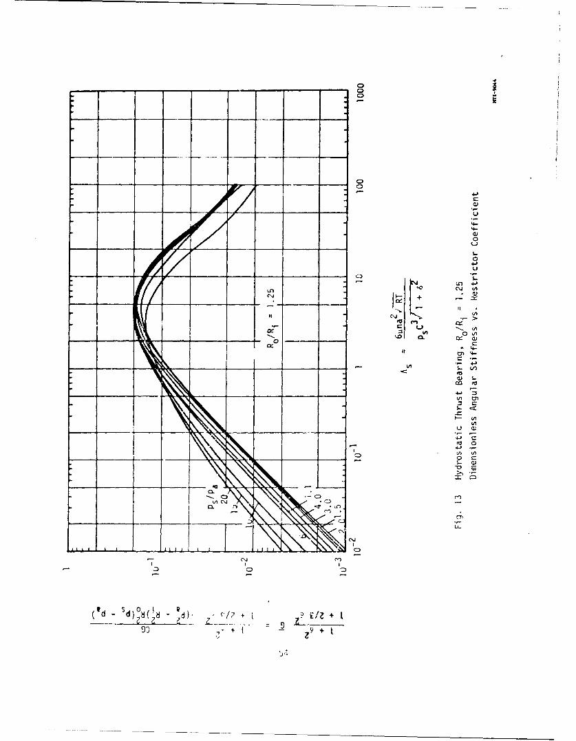
13. Hydrostatic Thrust Bearing, R /Ri - 1.25. DimensionlessAagular Stiffness vs. Restricior Coefficient .----------------------

14. Hydrostatic Thrust Bearing, R /Ri = 1.5. DimensionlessAngular Stiffness vs. Restric or Coefficient -----------------------

.15 Hydrostatic Tbrust Bearing, R /Ri = 2. DimensionlessS. Angular Stiffness vs. Restric or Coefficient ----------------------- 56

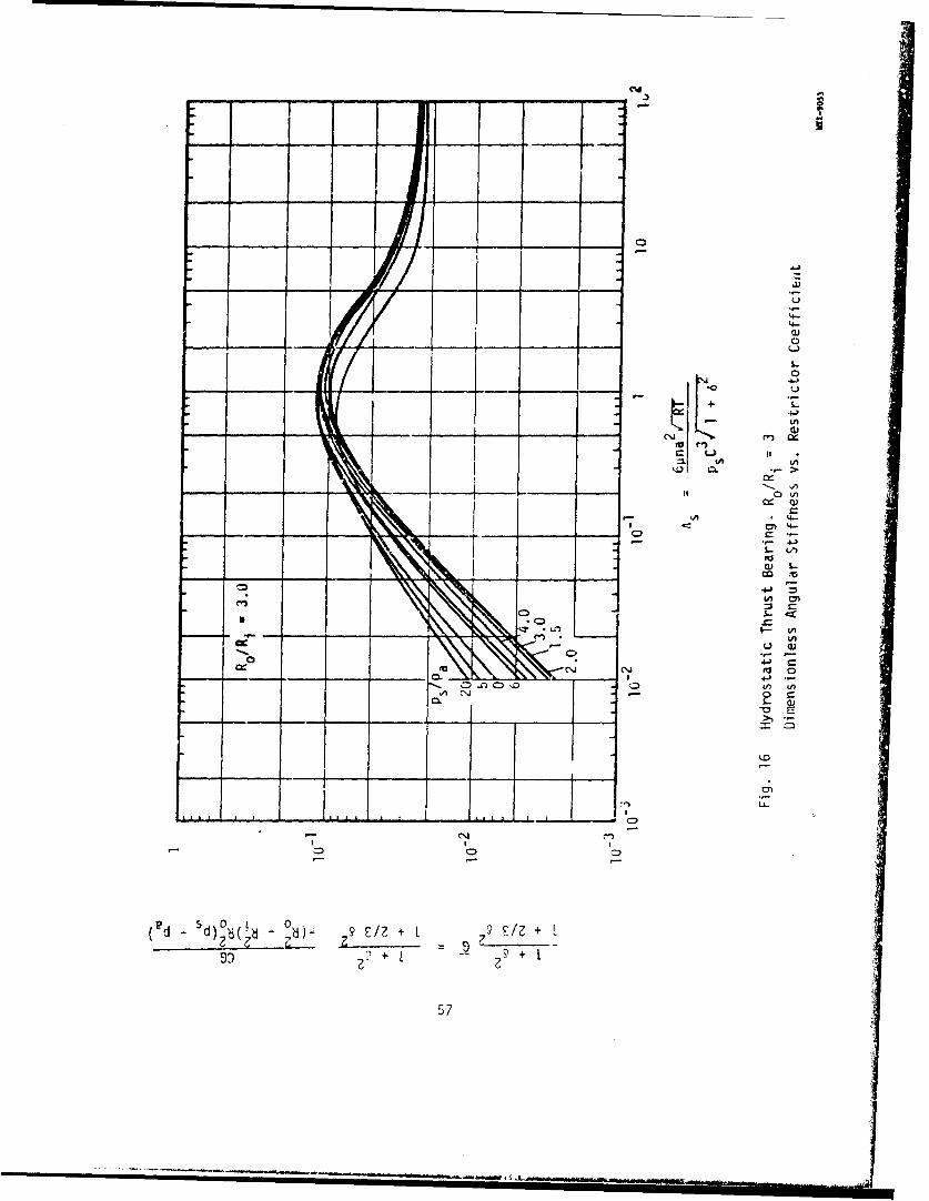
16. Hydrostatic Thrust Bearing, R /R = 3. DimensionlessAngular Stiffness vs. Restric or Coefficient ...............- 57

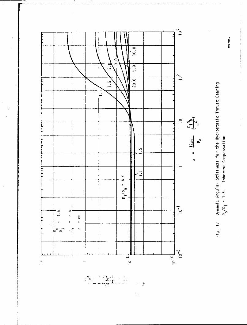
"17. Dynamic Angular Stiffness for the Hydrostatic ThrusLBearing R /R. = 1.5. Inherent Compensation ------------------------ 58

O 1

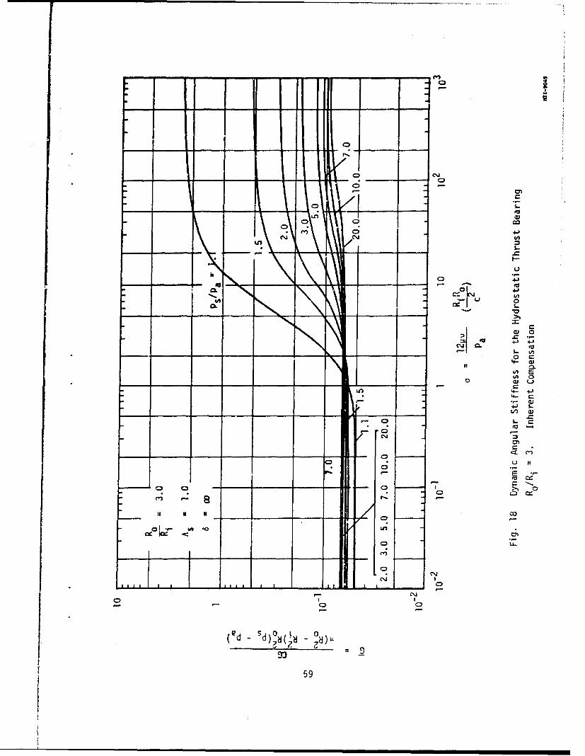
18. Dynamic Angular Stiffness for the Hydrostatic ThrustBearing R /R. = 3. Inhe:ent Compensation -------------------------- 59

O iM19. Minimum Number of Feeder Holes----------------------------------------60

vi

S/

SYMBOLS

a Orifice radius, inchiv-- a Dynamic influence coefficients

A Defined by Eq. (20)

B Single effective bearing damping, defined by Eq. (19),

lbs.sec/in

" major Maximum value of B, lbe-sec/in

-- Bmnor Minimum value of B, lbssec/in

"B-"n Bx, B yx,Byy Dynamic bearing damping coefficients, lbs.sec/inch

B Dimensionalized bearing damping coefficient

- GwB/P LZ

C Radial clearance, inch

D Bearing diameter, inch

D xxDxy ,Dyy Dynamic angular bearing damping coefficients,... lbs •sec • inch/radians

a Steady-state bearing eccentricity, inch

Fx ,Fy Bearing fluid film forces, lbs.

G, ,xG , G ,G Dynamic angular bearing stiffness coefficients,x, GXy Gy yy lbs•inch/radian

Ia{ }Imaginary part of complex expression

K Single effective spring qtiffness, deiined by Eq. (18),Wlb/in.

Knajor Maximum value of K, lb/in.

K minor Minimum value of K, lb/in.

K ,K ,K ,K Dynamic bearing stiffness coefficients, lbs/inchS.... xxxy yx yy

K Dimensionalized stiffness coefficient

- CK/PaLD

vii

ITI

L Bearing length, inch

L W~a1 'aaring span lanath, inch

SLJ + L2

LI Dista•ce from rotor C.G, to centerline of beatingnumber 1

L2 Distance from ro~or C.O, to oenterline of bearing2 number 2

M Journal bearing mass (half rotor mass for rigid votov)oibsmsec2/inoh

M Critical mass per bearing, isblsem /inch

M ,My x and y-oomponent of rotor banding moment to theX y left of a rotor mass station, lba'inoh

M'KM'Y x and y-component of rotor bending moment to they right of the rotor mass station, lbm~ineh

n Number of feeder holes

Ambient pressmuve psi&

P1 Bupply pressure, pei&

R 3earing radius, inch

Re{) Real part of complex ex;ression

R Outer radium of thrust bearing, inch

Ri Inner radius of thrust bearing, inch

2 2 0

T Temperature of Sas lubricantl•

t Time, msecond@

V )Vm x and y-component of rotor shear fovos to the loft

of a rotor mas• station, lbm.V1 ' V1 x and y-compontent of rotor shear force to the right

X y ofa rotor maes etation, ibs,

w Static loid on bearing, lbm.

viii

W'Wy External forces cn rotor in x and y direction, lbe.

*Z xx*Z X ,ZyxZ y Complex notation of stiffness and damping axial

coordinate, inch

Sxy Rotor amplitudes, inch

xcxIa Cosine and sine component of rotor x-amplitude, inch

ycDy$ Cosine and sine component of rotor y-amplitude, inch

- - a Axial coordinate, inch

Y - v/w, whirl frequency ratio

A Complex deterministic equation

c M RefA}, real part of complex equation

AM - Im(A), imaginary part of complex equation

25 M a /dC, inherent compensation factor

SB -M /C, eccentricity ratio for bearing

0 Angular displacement of thrust bearing in x-z plane,radian

"" M--j " , Compressibility number

.a2

2A 6sina 'V RT restrictor coefficient

8 w

JLubricant viscosity, lbs.sec/in2

v Whirl frequency, rad/sec

V Critical whirl frequency at threshold of instability,c rad/sec

a - , Squeeze number

ix

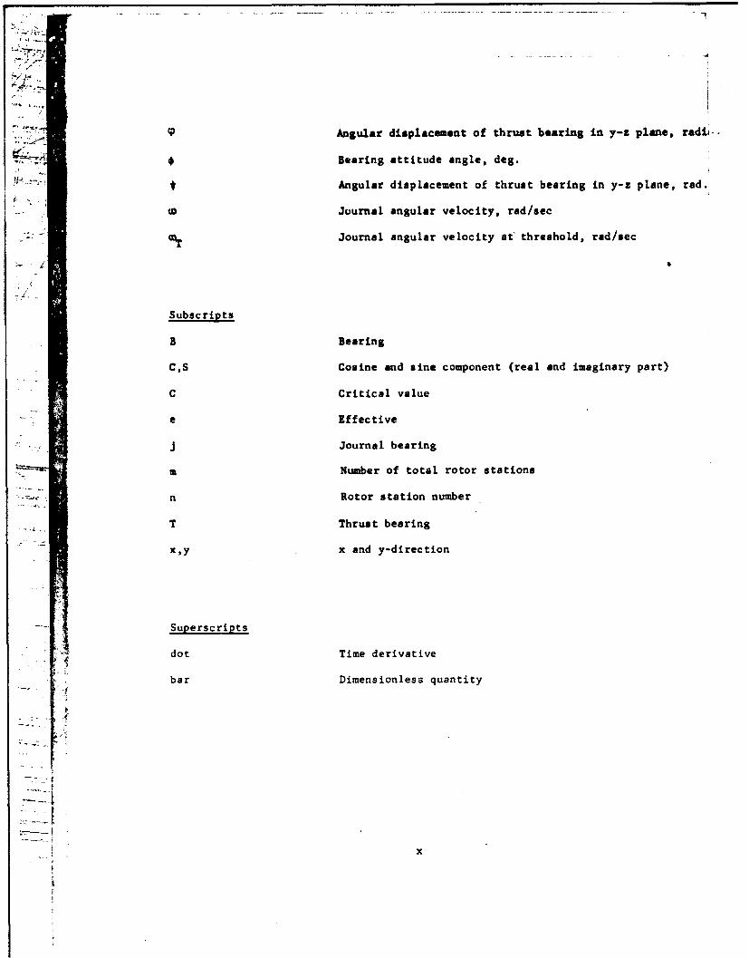
CAngular displacement of thrust bearing in y-z plane, radi-.

* Bearing attitude angle, deg.

* Angular displacement of thrust bearing in y-z plane, rad.

w Journal angular velocity, rad/sec

-T Journal angular velocity at' threshold, rad/sec

Subscripts

B Bearing

C,S Cosine and sine component (real and imaginary part)

C Critical value

e Effective

J Journal bearing

m Number of total rotor stations

n Rotor station number

T Thrust bearing

x,y x and y-direction

Superscripts

dot Time derivative

bar Dimensionless quantity

irx

SECTON I

NTRODUCTION

For rotors possessing * high degree of dissymmetry or for rather short rotors the

instability whirl motion will have a substantial conical whirl component. Under

such conditions the dynamic forces imposed on the rotor by the thrust bearing will

have an important effect on the dynamical characteristics and the stability of the

rotor-bearing system.

The purpose of the study described in this report was to develop the technology fo

determining effects of thrust bearing forces on the stability of rotors supported

in fluid film bearings and to assess the significance of this effect on rotors of

practical design. To this end, a computer program was developed to perform many

of the complex calculations necessary for determination of the stability limits of

complicated rotor-bearing systems which takes account of effects of thrust bearing

stiffness and damping. This computer program is an extension and modification of

a similar program developed in an earlier task performed under contract AF33(615)

3238 (Ref. 1). A complete description of the program including a computer listing

is provided in the present report.

The present report provides angular stiffness data for hydrostatic thrust bearing

geometries for use in the determination or rotor stnbility. Also a useful, simpli

fied method for determining stability of rotors supported on bearings all of which

are the same is described. Finally, several numerical examples of the calculation

of thrust bearing effects on rotor stability ate presented and the significance of

these effects is discussed.

Ai4

!I

SECTION 11

THE DETERMINATION OF THRESHOLD SPEED FOR WHIRL INSTABILITY OF A ROTOR

1. General Discussion

As is well established, a fluid film bearing supporting a rotor may be likened to

a spring-dashpot system in that the bearing reaction to small displacements may

be expressed in terms of stiffness and damping coefficients. A mass rupported by

springs has a number of natural spring-mass frequencies depending on the complexlty

of the spring system and the possible modes of motion of the mass. If any mode of

motion is excited at the natural frequency by an external harmonic force, then the

response of the system will be at a maximum but, if the system possesses effective

damping for this mode of excitation, then the response will be bounded and the sys-

tem will not be unstable. If, on the other hand, the natural frequency of a mode

of motion corresponds to a coadition where the effective damping of the system is

negative, then the motion of the system at that frequency will increase without

bound without any external excitation, and the system is considered as being un-

stable, i.e. subject to self-excited vibration. If a natural frequency occurs at

a condition of zero damping, then the system can be said to be at the threshold of

instability, where infinitesimally small exciting forces applied over a period of

time will result in ever increasing amplitudes of response.

The so-called critical speeds of a rotor-bearing system refer to resonant responses

of the system to unbalance forces of the system which, by their nature, are applied

at a frequency synchronous with the rotational speed cf the shaft. Since fluid filmbearings in general have positive damping to synchronous speed oscillations, criti-

cal speeds are not instabilities but simply represent a condition of large resonant

response to inherent unbalance forces. Fluid film bearings, however, do have an

effective damping to various modes of motion which does tend toward zero when the

motion occurs at some fraction of the running speed, usually at half the running

speed. Thus, as the running speed of a rotor increases beyond the first critical

speed or natural frequency speed, the rotor will begin to approach the condition

where the first resonant or natural frequency of the system will coincide with the

fractional frequer v at which effective damping goes to zero. When this coinci-

dence occurs, the rotor is said to have reached the whirl threshold speed. A

2

further increase in rotor speed usually results in a very rapid growth of whirl

amplitude and, in almost all cases, the whirl threshold speed represents the

upper limit for safe operation of the rotor.

We might note at this time that because effective damping of fluid film bearings

tends toward zero for half-frequency oscillations, the rule of thumb has arisen

that the threshold of instability is reached at about twice the first critical

speed of the rotor. The basis for this rule of thumb will be examined in more

detail in subsection 3 where there is discussed a procedure for using critical

speed maps for predicting threshold of whirl instability.

Having briefly discussed the qualitative nature of whirl instability and its dis-

tinction from critical speeds, we will now proceed to show the nature of the

linearized analysis required to determine the whirl threshold speed. In the

illustrative treatment below, we shall consider only the translatory mode of a

symmetric rotor supported on two identical bearings. The more general case of

the translatory, conical and bending modes of a non-symmetric rotor will be con-

sidered in subsection 2. For this general case, determination of whirl thresh-

old speed requires use of the computer program developed in this study. For the

simpler case presented below, whirl threshold speed can be determined analytically.

For the translatory mode of a rigid symmetric rotor the gravity and inertia

(D'Alembert) forces are equally borne by the two bearings. The kinematic rela-

tionships between the rotor and stator bearing surfaces at one bearing are at

every instant identical as those of the other. It is therefore only necessary to

consider the motion of one journal which has a mass equal to one-half the rotor

mass. Let the rotor mass be 2M and the journal center amplitudes be x and y.

At any given rotor speed and with a known static load on the bearing, the journal

center occupies a certain uniqtue equilibrium position relative to the bearing

center. When the journal whirls around its equilibrium position in a saiall orbit,

hydrodynamic bearing forces are generated in the bearing fluid film. These dy-

namic forces can be expressed in a linearized form by expanding the film forces

into a first order Taylor series. With the bearing fluid filk dynamic forces

represented by F and F and with the dynamic external forces on the rotor repre-x ysented by W and W as showt. in Fig. 1, the linearized equation of motion become:

x y

II

I.

w x

Fig. 1 Coordinate System for Fgrces anj Displacements

4

d2 x! H- - F +w -- K_ x-B i-K y-3 j+Wx

dt 2 x x xx x Xy xy

S(I)

dt2 Y Y " Kyy y B yy Y' " y

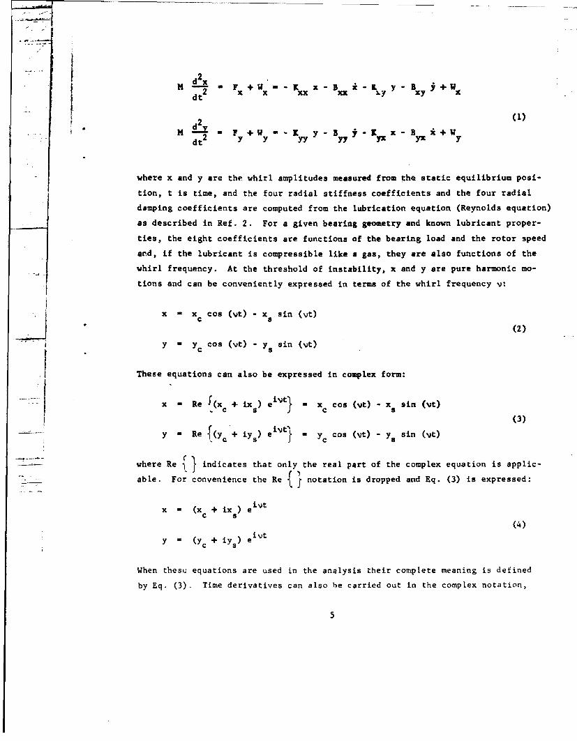
where x and y are the whirl amplitudes measured from the static equilibrium posi-

tion, t is time, and the four radial stiffness coefficients and the four radial

damping coefficients are computed from the lubrication equation (Reynolds equation)

as described in Ref. 2. For a given bearing geometry and known lubricant proper-

ties, the eight coefficients are functions of the bearing load and the rotor speed

and, if the lubricant is compressible like a gas, they are also functions of the

whirl frequency. At the threshold of instability, x and y are pure harmonic mo-

tions and can be conveniently expressed in terms of the whirl frequency v:

x - x Cos (Vt) - x sin (Gt)

(2)

y = Yc cos (vt) - y sin (vt)

These equations can also be expressed in complex form:

-X M Re ((x + ix ) eivt M x Cos (vt) - X sin (Vt)c s c a

! (3)

_.....abley : Re (Yc + iYs) eivt l :Y Cos (Vt) - y sin (Vt)

Swhere Re indicates that only the real part of the complex equation is applic-

.For convenience the Re notation is dropped and Eq. (3) is expressed:

x = (Xc + ix e ev

(4)

y (yc + iys) ei~

When thesu equations are used in the analysis their complete meaning is defined

by Eq. (3). Time derivatives can also be carried out in the complex notation,

5

bearing in mind that only the real part is of significance; e.g.

X Re ((x+ ix) ( eivt)3

a c

= Re (iv (x + ix ) eiVt'

- - vx sin vt - vx COS vtC 8

By differentiating Eqs. (4) and substituting into Eqs. (I) the equations of motion

can be written:

Mx-Z x-Zy+wxx xy Y x

(5)SMy - Z x -Z y+W

yx yy y

where:

-z K + iv Bxx (Similarly for Z y Zy, Zy)xx xx xy y yyS....(6)

af K +i•wBKxx +imBxx

y = v/l (7)

Here, w is the angular speed of rotation and y is the ratio of the whirl frequency

to the rotational frequency. In this form, the equations are equally valid for an

Lncompressible and a compressible lubricant. In matrix form Eqs. (5) can be ex-

pressed:

6

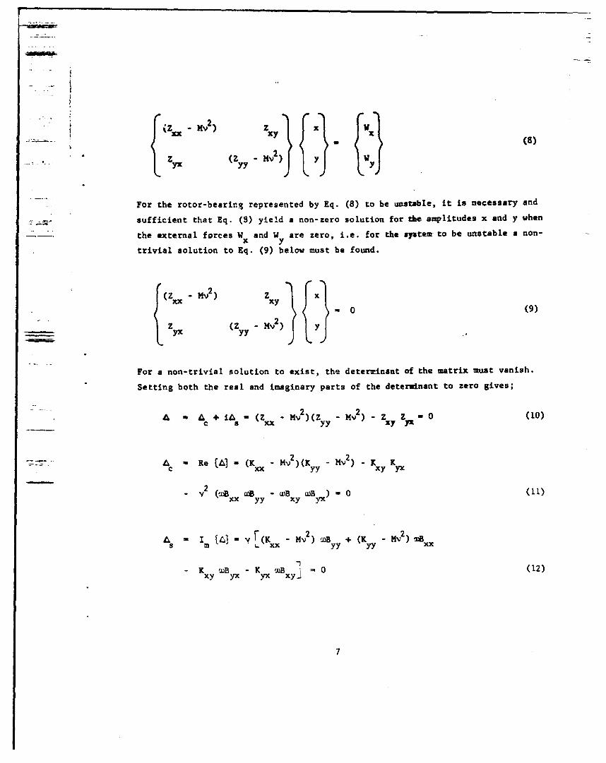
xXyI X (8)v)I1 I ii

'1Z2 (Z -M 2

For the rotor-bearing represented by Eq. (8) to be unstable, it is necessary and

--- sufficient that Eq. (8) yield a non-zero solution for the amplitudes x and y when

the external forces W and W are zero, i.e. for the system to be unstable a non-x ytrivial solution to Eq. (9) below must be found.

( - MV2) ( Z 0y (9Z ... 4zyy -MV 2)

For a non-trivial solution to exist, the determinant of the matrix must vanish.

Setting both the real and imaginary parts of the determinant to zero gives;

A - A + i& (Z - Mv2)(Z - Mv2)2 Z Z W - (10)C S xx yy 17,1x

A- = ReA (K - MV2 )(KY -Mv 2 )- K Kyx

- 2 (,iBBx wB - wB w•Byx)-0 (11)yy xy yx

- Y (K - MV.2 ) a + (K -•M) 2ass m yy x

- K ,BuBxy] = 0 (12)" Kxy myx yxy7

"Thus, when both the real and imaginary parts of the determinant vanish simultan-

eously harmonic motion or whirl is present and this whirl is referred to as rotor

instability. Every combination of y and co satisfying either Eq. (11) or Eq. (12)

can be represented by a point in a y-w plot. Typically the locii of these points

appear as shown in Fig. 2.

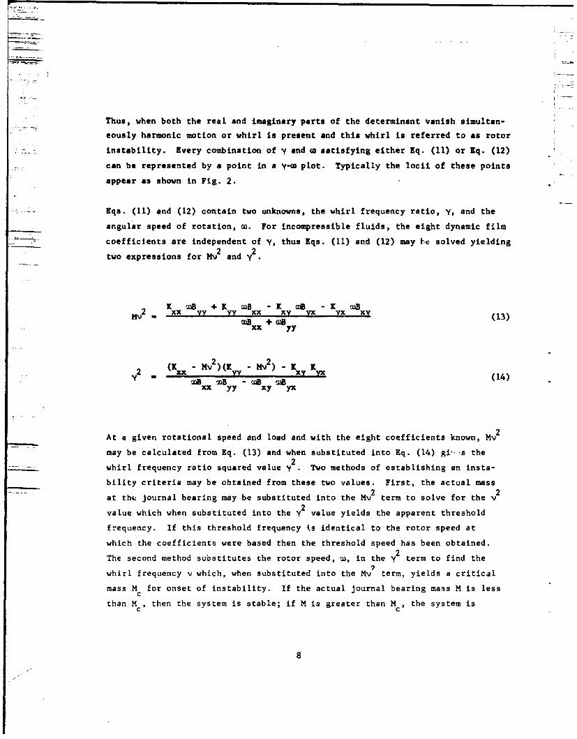
Eqs. (11) and (12) contain two unknowns, the whirl frequency ratio, y, and the

angular speed of rotation, w. For incompressible fluids, the eight dynamic film

coefficients are independent of y, thus Eqs. (11) and (12) may he solved yielding

two expressions for MV2 and 2

2 • +K •uB -K aB -KI~MV2 xx Vy Vy xx xy yX ,x (13)

+ axx yy

2 (Xxx - M2 )(K - MY ) - K xy Kyx= , mB - •BX at (14)xx yy xy yx

At a given rotational speed and load and with the eight coefficients known, MV2

may be calculated from Eq. (13) and when substituted into Eq. (14) gi- Is the2

S. whirl frequency ratio squared value y . Two methods of establishing an insta-

bility criteria may be obtained from these two values. First, the actual mass

at the journal bearing may be substituted into the MV2 term to solve for the v22

value which when substituted into the y value yields the apparent threshold

frequency. If this threshold frequency ts identical to the rotor speed at

which the coefficients were based then the threshold speed has been obtained.2

The second method substitutes the rotor speed, w, in the y term to find the

whirl frequency v which, when substituted into the M% term, yields a critical

mass M for onset of instability. If the actual journal bearing mass M is lessc

than MC, then the system is stable; if M is greater than M c, the system is

8

unstable. The mathematical derivation of this stability criterion is given in

R.ef. 4. _

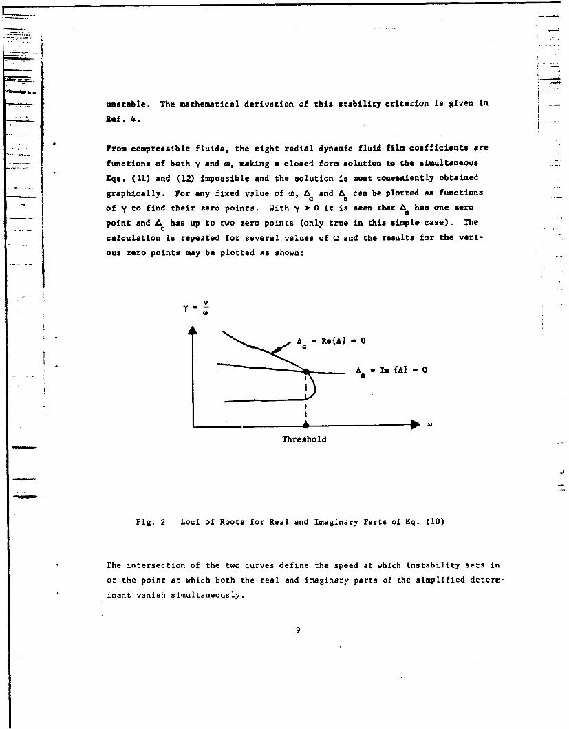
From compressible fluids, the eight radial dynamic fluid film coefficients are

functions of both y and w, making a closed form solution to the simultaneous

Eqs. (11) and (12) impossible and the solution is most conveniently obtained

; j graphically. For any fixed volue of w, A and A can be plotted as functionsc

of y to find their zero points. With y > 0 it is seen that As has one zero

point and A has up to two zero points (only true in this simple case). Thec

calculation is repeated for several values of co and the results for the vari-

ous zero points may be plotted As shown:

V

'a)

a A 0I.AJ-oc5

Threshold

Fig. 2 Loci of Roots for Real and Imaginary Parts of Eq. (10)

The intersection of the two curves define the speed at which instability sets in

or the point at which both the real and imaginary parts of the simplified determ-

inant vanish simultaneously.

9

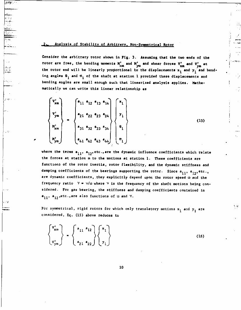
2,. Analysis of Stability of Arbitrary. Non-Symmetrical Rotor

Consider the arbitrary rotor shown in Fig. 3. Assuming that the two ends of the"rotor are free, the bending moments H' and M' and shear forces V' and V' at

Xm yM xI ymthe rotor end will be linearly proportional to the displaceuients.xl and*y' And bend-

ing angles 01 and 0 of the shaft at station I provided these displacements andbending angles are small enough such that linearized analysis applies. Mathe-

matically we can write this linear relationship as

"---xm 11 12 13 14 1

VM 21 22 23 a24 Y1

(15)

xm 31 32 33 834 1

pm0 a' 412 43844) 1.

where the terms all, a 1 2 , etc.,are the dynamic influence coefficients which relate

the forces at station m to the motions at station 1. These coefficients are

function3 of the rotor inertia, rotor flexibility, and the dynamic stiffness and

damping coefficients of the bearings supporting the rotor. Since aill a 1 2 ,etc.,

are dynamic coefficients, they explicitly depend upon the rotor speed t and the

frequency ratio Y - v/' where v is the frequency of the shaft motions being con-

sidered. For gas bearing, the stiffness and damping coefficients contained in

aill a812,etc.,are also functions of wn and Y.

For symmetrical, rigid rotors for which only translatory motions x1 and y1 are

considered, Eq. (15) above reduces to

xm a 11 312 1

Vyim <a21 a22) (Y11

10

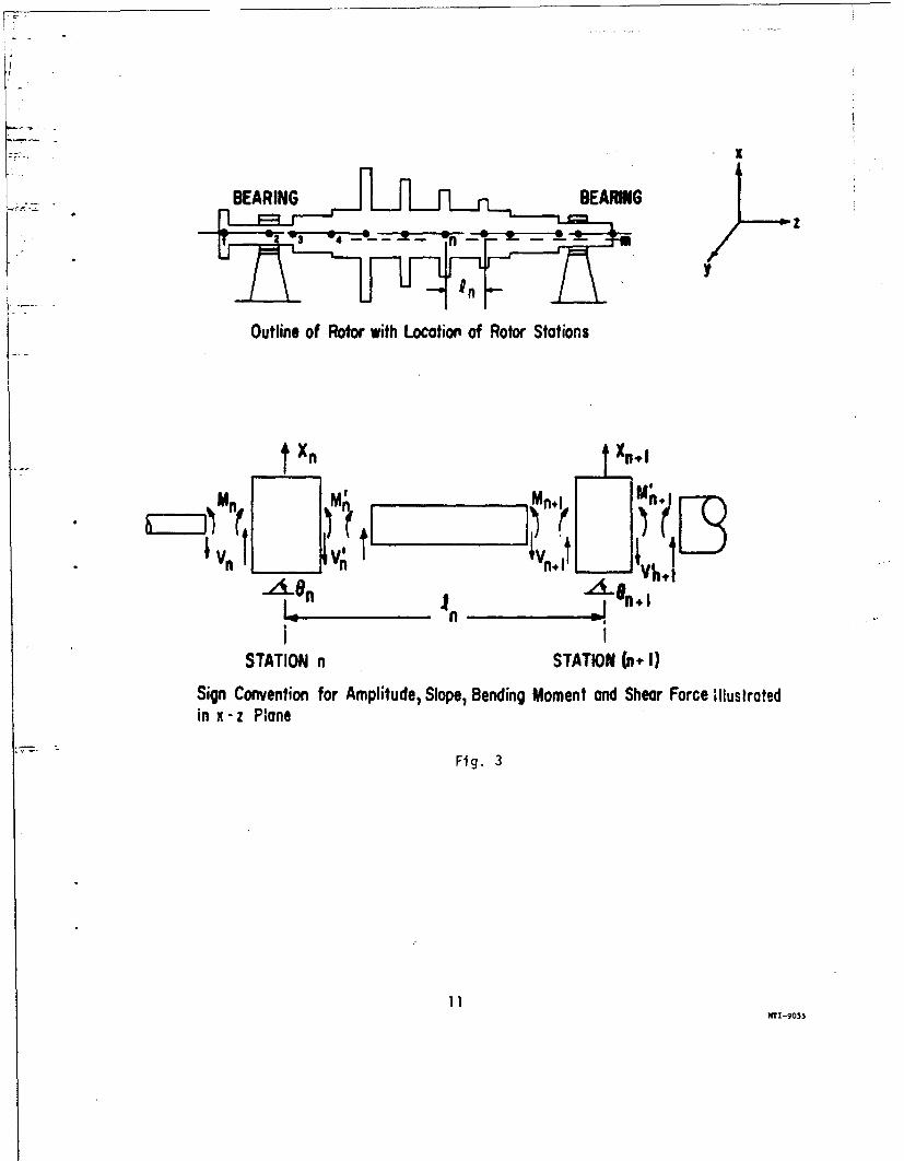
y

Outline of Rotor with Location of Rotor Stations

Xn .•-0n.1

i I

STATION n STATION (n I1)

Sign Convention for Amplitude, Slope, Bending Moment and Shear Force illustratedin x -z Plane

Fig. 3

N'1-9055

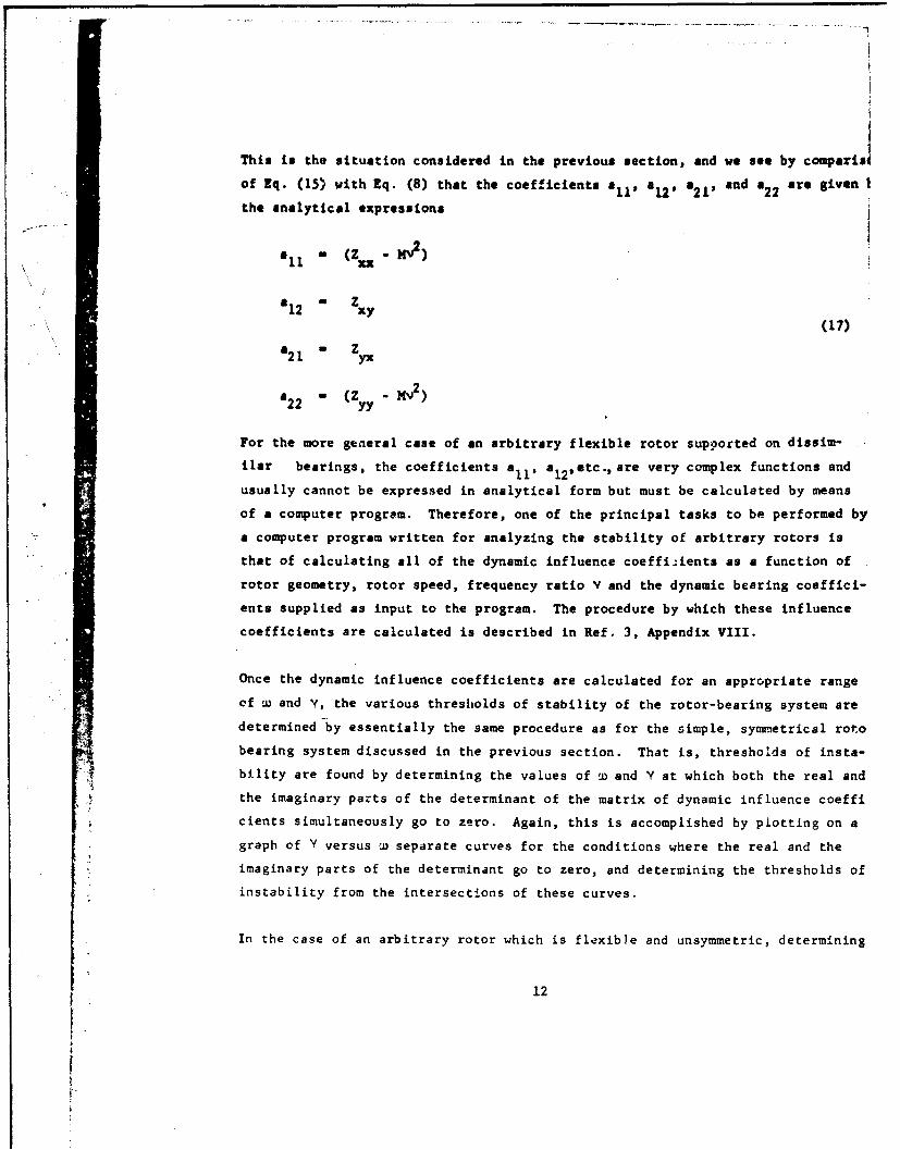
This is the situation considered in the previous section, and we see by comparial

of Eq. (15) with Eq. (8) that the coefficients a11 , '12' a2 1 , and '22 are given [

the analytical expressions

a~ (Z~ -!V2)"ll " (

S12 Zxy

(17)

a 21 Z21 yx

a 2 2 - (Z - Mv2)

For the more general case of an arbitrary flexible rotor supported on dissim-ilar bearings, the coefficients all' a12 , etc., are very complex functions and

usually cannot be expressed in analytical form but must be calculated by means

of a computer program. Therefore, one of the principal tasks to be performed by

a computer program written for analyzing the stability of arbitrary rotors is

that of calculating all of the dynamic influence coeffizients as a function of

rotor geometry, rotor speed, frequency ratio Y and the dynamic bearing coeffici-

ents supplied as input to the program. The procedure by which these influence

coefficients are calculated is described in Ref. 3, Appendix VIII.

Once the dynamic influence coefficients are calculated for an appropriate range

of w and Y, the various thresholds of stability of the rotor-bearing system are

determined by essentially the same procedure as for the simple, symmetrical roto

bearing system discussed in the previous section. That is, thresholds of insta-

bility are found by determining the values of w and Y at which both the real and

the imaginary parts of the determinant of the matrix of dynamic influence coeffi

cients simultaneously go to zero. Again, this is accomplished by piotting on agraph of Y versus a) separate curves for the conditions where the real and the

imaginary parts of the determinant go to zero, and determining the thresholds of

instability from the intersections of these curves.

In the case of an arbitrary rotor which is flexible and unsymmetric, determining

12

k

the real and imaginary parts of the determinant of the matrix of influence coef-

ficients cannot, in general, be accomplished analytically but must be accomplished

numerically by the computer program for analyzing stability. The procedure is

essentially one of having the computer program calculate the values of the real

and imaginary parts of the determinant over a specified range of whirl frequency

ratios at a fixed rotor speed. The program then determines the zero points of

the real and imaginary parts of the determinant by quadratic interpolation each

time a change in the sign of these functions occurs. It should be clearly noted

here that the computer program itself does not determine thresholds of stability;

this remains to be accomplished by the designer by plotting the curves of the

loci oi the real and imaginary roots of the stability-determinant.

The discussion presented above serves to. describe in a qualitative way the nature

of the process of determining the stability of an arbitrary rotor and how this

process is implemented by means of a computer program. A detailed description of

thL. computer program developed in the present project for the purpose of analyzing

rotor-bearing stability is given in Appendix I.

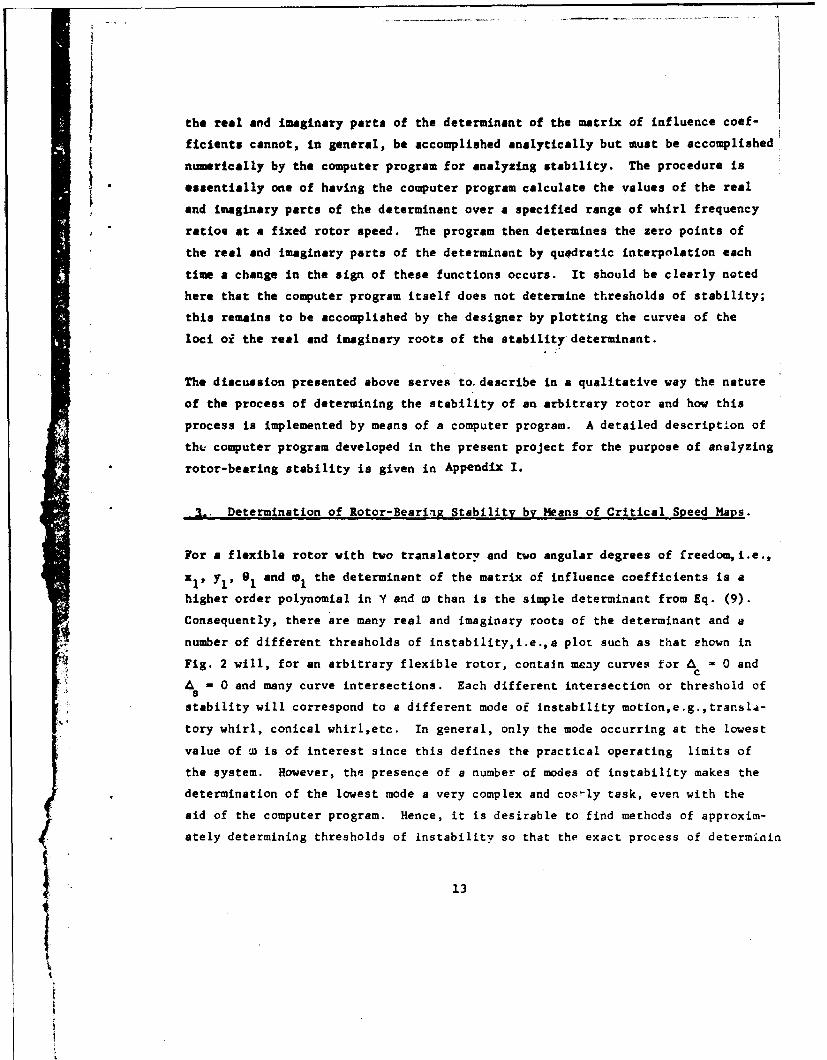
3.. Determination of Rotor-Bearing Stability by Means of Critical Speed Maps.

For a flexible rotor with two translatory and two angular degrees of freedomi.e.,

Xl, Yl' 1 and t1 the determinant of the matrix of influence coefficients is a

higher order polynomial in Y and w than is the simple determinant from Eq. (9).

Consequently, there are many real and imaginary roots of the determinant and a

number of different thresholds of instability,i.e.,a plot such as that shown in

4 Fig. 2 will, for an arbitrary flexible rotor, contain many curves for 4 - 0 andc

A - 0 and many curve intersections. Each different intersection or threshold of4 sstability will correspond to a different mode of instability motion,e.g.,transla-

tory whirl, conical whirl,etc. In general, only the mode occurring at the lowest

value of w is of interest since this defines the practical operating limits of

the system. However, the presence of a number of modes of instability makes the

determination of the lowest mode a very complex and cos~ly task, even with the

aid of the computer program. Hence, it is desirable to find methods of approxim-

ately determining thresholds of instability so that the exact process of determinin

13iI.

S.

such thresholds by means of the stability program can be accomplished with a

minimum of costly searching.

One convenient approach for approximately locating the instabilities of most

rotors can be had by use of a critical speed map for the rotor in question. A

critical speed map shows the various natural or resonant frequencies of a rotor

as a function of a single value of spring stiffness K assigned to the bearin3s

supporting the shaft. A typical critical speed map is shown in Fig. 10. For

complex rotors, such maps are usually obtained by means of a computer program

written specifically for this purpose.

As was discussed earlier in subsection 1., whirl instability can be viewed as

a condition of undamped resonance. In particular Lund (Ref. 4) has shown that

if this view point is taken, then at the threshold of stability the fluid film

beering can be represented by a single effective spring stiffness coefficient

K and damping coefficient B given by

1 11 4 (K x- K Y) (-UB D - YjB YX) +-(K xyYjB X+ K YXYDB )

K -- (K + K xx v xx v 2xv x v v2 xx yy A

(18)

B -!(YWu + YB )-A (19)2 xx ÷ yy

where A is expressed by the following quartic equation:

A 1(' -K) K K -1 ~(-YwBxx tByy 2 _ N4Bx Y-uB] A 24 xx yy yx 4 xx yy xy •yx]

)Y8 - 1 (K tB +K =Y-B 2 04 Kxx" yy)(•x -X YByy ÷Y + 2 xy •OyX yx Yxy

(20)

14

I

Since B is real, Eq. (20) has only two solutions for A which are of equal magni-

tude but of opposite sign. In order for the effective bearing damping to become

zero (corresponding to the undamped resonance criteria) at some value of Y, then

A must be positive from Eq. (20) since (y.Bx + YwB y ) is always positive. There-

fore, only the real, positive value of A is used to define the stiffness coef-

ficient in Eq. (18).

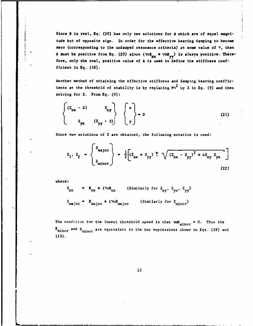
Another method of obtaining the effective stiffness and damping bearing coeffic-

ients at the threshold of stability is by replacing Mv2 by Z in Eq. (9) and then

solving for Z. From Eq. (9):

Z~~ (ZzJ \ 0~~m (21)z YX (Z - z)J Y

Since two solutions of Z are obtained, the following notation is used:

-major+ 4Z Zzl, z2 - ( Z + z:rL (Z -Z + 4xy z 1l[minor 2

(22)

where:

Z - K + iYcuB (Similarly for z , z )

Zmajor n Kmajor + iYDBmajor (Similarly for Zminor)

The condition for the lowest threshold speed is that 'yLminor - 0. Thus the

Kminor and Bminor are equivalent to the two expressions shown in Eqs. (18) and

(19).

15

In arriving at a Kminor and a Bminor value, the negative sign in front of theradical in Eq. (22) is generally used. An evaluation of the value of the rad-

ical is somewhat difficult since the coefficients of the bearing change con-

stantly with increasing eccentricity. Various bearing types and coefficients

have been evaluated and this sign convention has proven correct. This sign

convention is also consistent with the analysis by Lund (Ref. 4).

The importance of Kminor lies in the convenience with which it can be used in

conjunction with a rotor critical speed map to determine the onset of insta-

bility. By cross-plotting the minor stiUness of the bearing as a function

of rotor speed, several critical speed curves may be crossed before the rotor

design speed is reached. The threshold speed is obtained when the first crit-

ical speed corresponding to Kminor' divided by the critical whirl frequency

ratio y, gives the rotor speed at which the Kminor and y were evaluated. The

critical whirl frequency ratio is defined as the value of v/u at which B eval-

uated from Equation (191 goes to zero. In most instances, the critical fre-

quency ratio is nearly 1/2, and since K mnor tends not to change very rapidly

with rotor speed, this gives rise to the rule of thumb that the whirl threshold

speed is approximately twice the first critical speed of the rotor bearing system.

The critical whirl frequency ratio can be determined from Eq. (14).

The specific steps involved in determining threshold speed from a critical speed

umap are as follows:

(1) Obtain a critical speed map of the rotor as a function of support

stiffness.

(2) Calculate the eight radial bearing coefficients over some specified

speed range which one estimateswill contain the whirl threshold speed.

(3) Compute the K minor and y values from Eqs. (18) or (22) and (14), for

various shaft speeds.

16

/

J (4) For each of the Kminor values, enter the critical speed map at each

value and obtain the first natural frequency or critical speed.

(5) For each shaft speed selected divide the critical speed by the com-

puted whirl frequency ratio. When the resulting speed, which we shall

refer to as apparent threshold speed, equals the shaft speed at which

the X value was evaluated, then the actual threshold speed has

been determined.

For incompressible lubricated bearings the stiffness and damping coefficients

are independent of the whirl frequency ratio, whereas the compressible lubri-

i cated bearing coefficients must be obtained at the critical whirl frequency

ratio. In general these gas bearing coefficients may be obtained at v/4) - 0.50

with suf'icient accuracy since the critical whirl frequency ratib is ujually

-lose to this value.

It should .e noted that use of a critical speed map together with values of

Kminor to determine the stability threshold is valid for rotors of •trary

shape and flexibility but does rely upon the bearings supporting the rotor

being quite similar, since the critical speed map is plotted in terms of only

one value of bearing stiffness. However, if the bearings supporting the rotor

are not too dissimilar, the present approach will serve to indicate at least

approximately the critical speed and critical speed ratio by using values of

Sminor for any one of the bearings. A more exact value for critical speed can

then be determined by using the computer program developed for calculating

rotor bearing stability.

An example calculation of how to determine whirl threshold speed from a crit-

ical speed map is given in the next section.

17

SECTION III

EFFECT OF THRUST BEARING STIFFNESS AND DAMPING ON ROTOR-BEARING STABILITY

1. Discussion

Since a thrust bearing exhibits no radial stiffness or radial damping properties,

the threshold speed of a rotor which whirls in the lateral or radial mode will

not be affected. However, if the rotor motion is angular or conical, considerable

restraint can be imposed on the rotor by the angular thrust bearing properties.

Thus, if the lowest critical speed of the rotor is conical, the threshold speed

of the rotor could be significantly influenced by the addition of the thrust bear-

ing coefficients. The computer program described in Appendix I of this report

allows for the inclusion of these thrust bearing coefficients. In this present

section we will consider some simplified relations which enable us to estimate

the effects of thrust bearing stiffness on the conical stability of a symmetric

rotor.

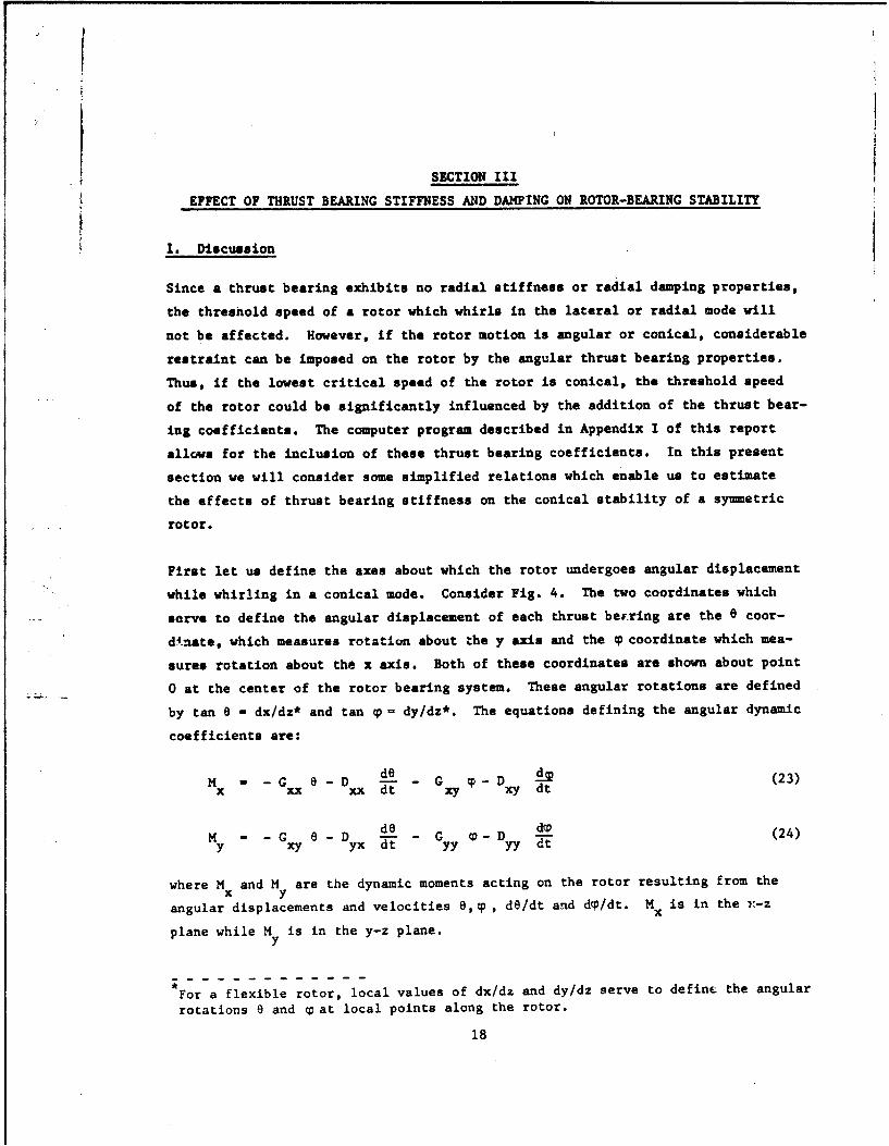
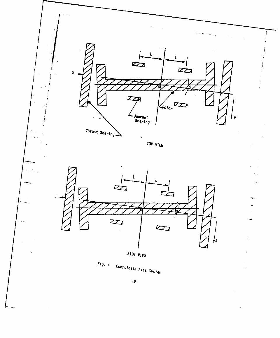
First let us define the axes about which the rotor undergoes angular displacement

while whirling in a conical mode. Consider Fig. 4. The two coordinates which

serve to define the angular displacement of each thrust berring are the e coor-

d•nate, which measures rotation about the y axis and the c coordinate which mea-

sures rotation about the x axis. Both of these coordinates are shown about point

0 at the center of the rotor bearing system. These angular rotations are defined

by tan 8 = dx/dz* and tan c = dy/dz*. The equations defining the angular dynamic

coefficients are:

Mde - G-Gp -DD .4-D(23)x xx xx dt xy xy dt

M - - G e - D_ dt - G o- D (24)y xy yx dt yy yy dt

where M and M are the dynamic moments acting on the rotor resulting from thex yangular displacements and velocities 8,c p, de/dt and df;/dt. Mx is in the 7:-z

plane while M is in the y-z plane.y

For a flexible rotor, local values of dx/dz and dy/dz serve to define the angular

rotations e and c at local points along the rotor.

18

I zz

SIDEp VIEW

Fi.~ COOrdinate Axis SYstem

.19

The comquter program written to analyze rotor-bearing stability accepts the eight

angular stiffness and damping coefficients Gxx, ,D , G xy, etc.,directly as bearing

input data along with the translatory coefficients Kxx, MBxx, Kxy, etc. However,

in order to gain an estimate of the effect of thrust bearing angular stiffness on

rotor-bearing stability, it is convenient to try to use the critical speed map ap-

proach for determining whirl-instability that was described earlier in the report.

To use this approach, it is necessary to relate the thrust bearing angular coef-

ficients to effective translatory stiffness and damping coefficients of the journal

bearings supporting the rotor. For a symmetrical rotor-bearing system this can be

accomplished by the following geometrical considerations. Referring to Fig. 4 we

see that the restoring moment (HX ) in the x-z plane exerted by each journal bear-

ing in response to a static angular displacement 9 about an axis through the point

0 parallel to the 0 axis is

(M) - - KxxL2 2 (25)

Similarly, the restoring moment (My)J, due to each journal bearing is

(My) - K L2 9 (26)

On the other hand, the restoring moments (Mx)T and (My)T exerted by each thrust

bearing due to the angular displacement 0 are given by Eqs. (23) and (24),i.e.,

(MHx)T - G xx (27)

(My)T = - G yx (28)

Therefore, we see that for angular displacement in this symmetrical system, the

restoring moments of chrust bearings can be represented simply by adding the

"effective" stiffness coefficients G xx/L2 and G yx/L2 respectively to the existing

coefficients K and K of the journal bearings. This applies as well to all ofxx yx

the stiffness and damping coefficients. This, for angular displacements about

axes through the point 0, the restoring moments can be determined by assuming

that each journal bearing has effective stiffness and damping coefficients (K xx)e

20

(Bxx)e, (Kxy)e ,etc.,given by

(Kx )e - x + /G x/2

(Kye - Kxy + G yIL2

(Kyx)e y Kx+ Gyx/L2

(Kyy e yy yy(29)

(Bxx)e B Bxx +4 xx/L

2

B L2

(B )e- + D ALlye Xy xy

:x(Bx e v xyx

(B) - B + D /L 2yy e yy yy

The approach of taking account of thrust bearing effects on conical motions of

symmetrical systems by means of adding effective stiffness and damping to existing

journal bearings permits one to use the critical speed map method for estimating

whirl instability as described in the previous section. This would be accomplished

-.... by using the total effective values of stiffness for conical motion of the rotor,

as defined in Eqs. (29) to -tvaluate Kminor and overall damping B as defined by

Eqs. (18), (19) and ( Note that this procedure is valid for conical whirl

instability only. Thrust bearings would have no effect on the '.ranslatory whirl

mode and their angular coefficients should not be included in the evaluation of

Kminor and B if this mode of instability is being determined.

Some sample calculations were performed by the critical speed map methoa to ex-

amine the effect of independently adding principal angular stiffness, Gxx dnd Gyy

and principal angular damping D and D on the conical stability of a symmetricalxx yy

rotor. The conclusions reached were that:

21

(1) Addition of principal angular stiffnesses G and G does not changexx yy

the critical value of frequency ratio Y for instability but can in-C

crease the threshold speed wo for instability by isicreasing the naturalC

frequency of the conical mode.I

(2) Addition of principal angular damping, D and D , does not change thexx yynatural frequency of the rotor-bearing system, but does decrease the

critical frequency ratio for instability (i.e., the frequency ratio atwhich damping B goes to zero) thereby increasing the threshold speed Wo

at which instability occurs.

In the sub-section below are discussed various specific design examples for which

the effect of thrust bearings on rotor-bearing stability are investigated.

2. Sample Calculations

The basic tool used in computing the threshold speed is computer program PN400.

With this program it was pcssible to obtain the threshold speeds exactly with

and without the thrust bearing effects. However, since much time searching forthreshold speeds is generally required when using this program alone, the shorter

critical speed map technique for locating threshold speeds, outlined in this re-port, was first used to obtain an approximate value of threshold speed with an

exact solution being then obtained using the computer program.

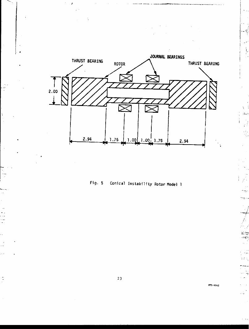
Two rotors will be analyzed to determine their threshold speeds with and without

the addition of a thrust bearing system. These two rotor models are shown in

Figures 5 and 6.

The first rotor, Figure 5, weighs approximately 7.2 lbs. and is supported by twogas-lubricated hydrodynamic journal bearings. The load is identical on each bear-

ing. Air at 1000 F and ambient pressure (14.7 psia) is supplied to each bearing.

Thrust bearing surfaces are available at either end of the rotor.

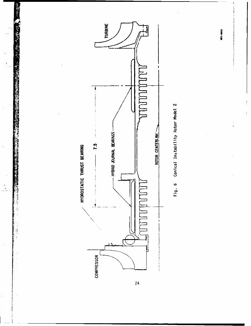
The second rotor, Figure 6, weighs approximately 18.75 lbs. and is supported by

22

JOURNAL BEARINGSTHRUST BEARING ROTOR THRUST BEARING

2.00

I-I

2.94 1. 75 1.001-1.0011.75 J~ 2.94

Fig. 5 Conical Instability Rotor Model 1

/A-

23

MT7I-9042

4-J

4 JJ

CD tJ to

0

w C

24

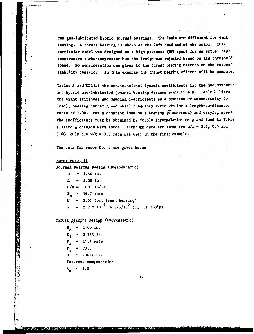
two gan-lubricated hybrid journal bearings. The leads are different for each

bearing. A thrust bearing is shown at the left hand end of the rotor. This

particular model was designed as a high pressure (U) spool for an actual high

temperature turbo-compressor but the design was rejected based on its threshold

speed. No consideration was given to the thrust bearing effects on the rotors'

stability behavior. In this example the thrust bearing effects will be computed.

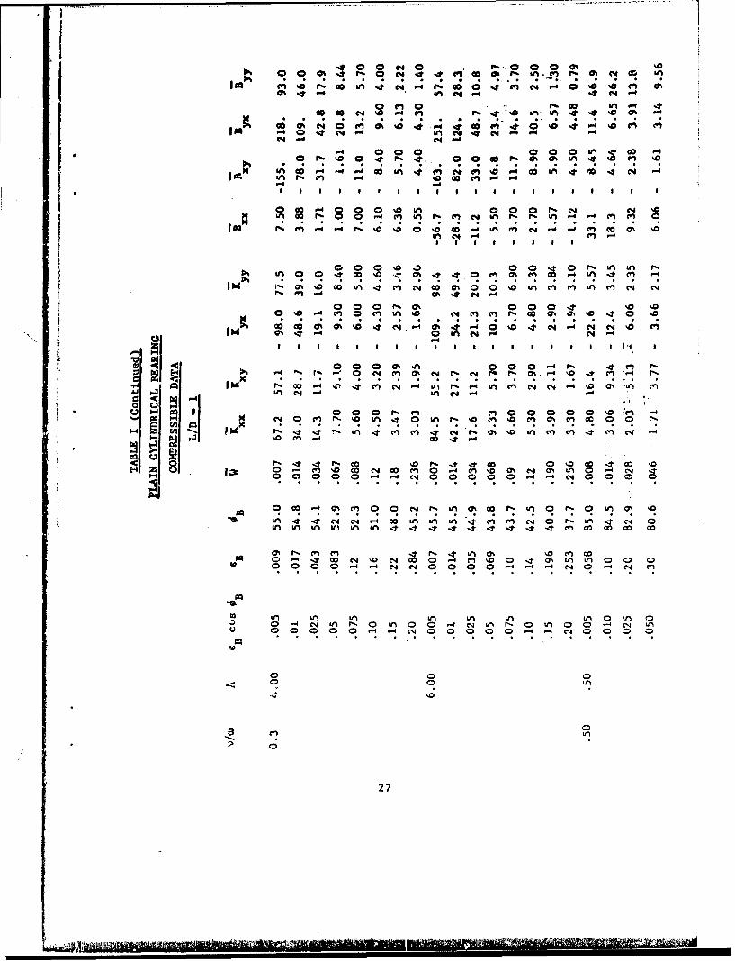
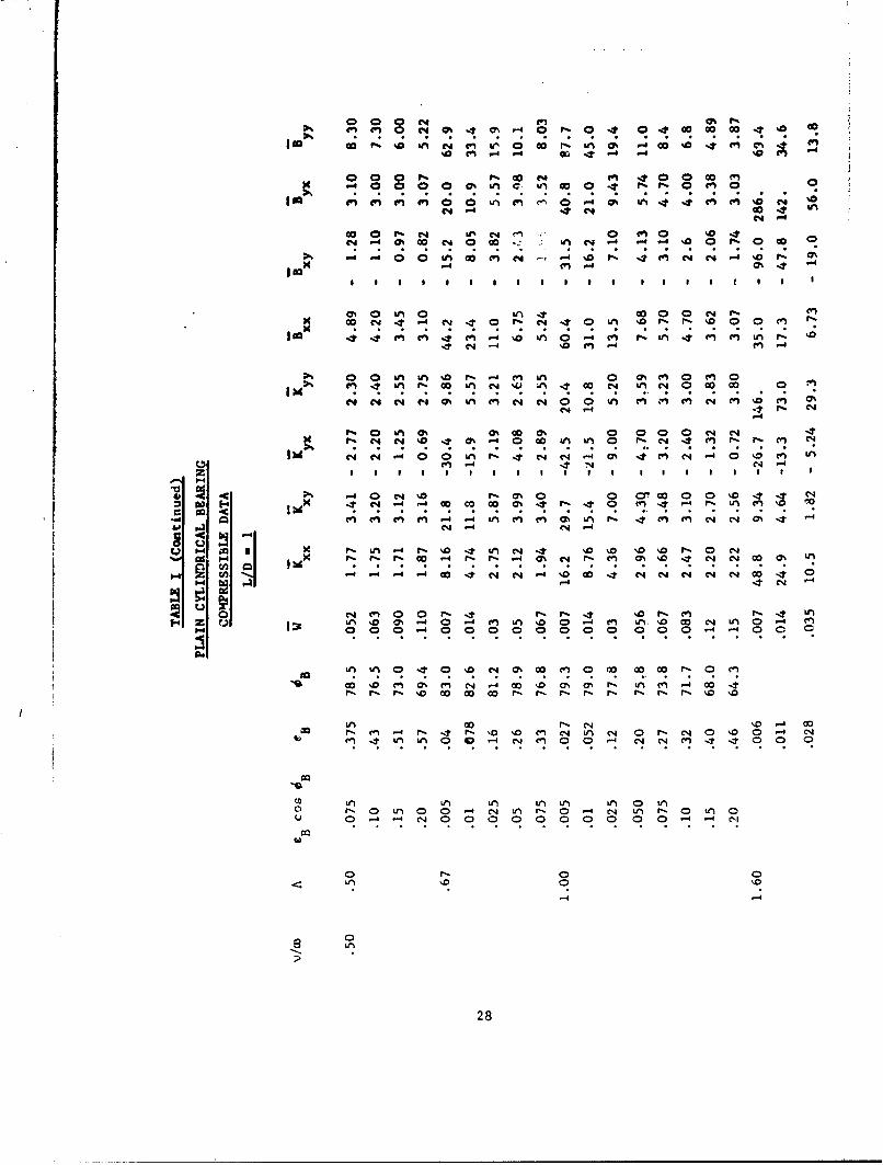
Tables I and 1 list the nondimensional dynamic coefficients for the hydrodynamic

and hybrid gas-lubricated journal bearing designs respectively. Table I lists

the eight stiffness and damping coefficients as a function of eccentricity (or

load), bearing number A and whirl frequency ratio v/6 for a length-to-diameter

ratio of 1.00. For a constant load on a bearing aconstant) and varying speed

the coefficients must be obtained by double interpolation on A and load in Table

I since A changes with speed. Although data are shown for v/w - 0.3. 0.5 and

1.00, only the v/w - 0.5 data was used in the first example.

The data for rotor No. 1 are given below

Rotor Model #1

Journal. BearFing. Design (Hydrodynamic)

D - 1.50 in.

L - 1.50 in.

C/R - .001 in/in.

P a 14.7 psiaa

W , 3.62 lbs. (each bearing)

- 2.7 X 10-9 Ib.sec/in2 (air at 100OF)

Thrust Bearing Design.(Hydrostatic)

R - 1.00 in.0

Ri = 0.333 in.

P - 14.7 psiaa

P = 73.5S

C = .0011 in.

Inherent compensation

As = 1.0

25

-I,

0 4 C2~ IAO 1% 4 Cý C- V! 0

M VI M M r'-%' at% *0 000 0 0

"P4 "4 "-4 en N4 N4 "4 o C"A - 0 m N , % 4 (AIca "4 CA 1 4 In LA N 4

00 C~) LA %D 03 "4 4 '00 A 4

(A(fn A4ol(invi "4 0 N "4 4 n N t LA 4 40 g 0 4 4 N 4"

00 0 C14 0 0 NO 00 00 cor5 % *4 (n LA LA 4n 4ý C4 4 A 1% N 0 T Go %0

C .~ 4 N ý N .N 4 N N 0 0 4 -AN C4 44 A C',uNC

"14 "4C4P. (

0OI en 000 r- 0 00 (Ac

"C4 LA0"4 . n 00 N% en It ON c 0 W) N #4

z I 43% N4 4 43% Ný "4

pa3 14 C4V 0 00 NA 0 0 Ln LA 0 %0 "4to C4 4 (A N N 0 T 0%h r% 0 4 LA N4 00 4 "4 0 N4 Le) r%

14x (n (A vA (A (A (A Ný N A "4' 0 4 4 (4 NI4t

in LA (Al %0 N% 0 , 00 0m0 (

1-4 0 LA LA LAAN"0 '00 14 rN 'A NA014 ~~ ~C "4 "4 - 4 N N 4 N ( 4 LA N 4 3% C4L A (A (

Z~~ ~ ~ C0 Nn " -c4 N. %0 N "4"H In"4s % 0 4 L 4 MM l c n 0

00wNo (A 00% (Am 4 LAN 3% 4 N

go M 0 l "4 0 C14 "4 00 0 04 0 0 Le 0 o 0 4 "4 "

LA 0A 403 0 (A 440 C)0 LA

10

A C0 '- 0 L 0 "4% L

14 c

* nL

o 0 AO 3 0 L O 3% 0 LA

0% In P4 S-i - % 0 04 C4N- 0 0 % 04

r4 P4N 4 V4

00~~i Go4 4%ýin i 44~Go

0o N 4 An Go Nn -4C

G4in o -4 '- - 0 i 4 4~40 C) %a 40.C 4 C4

go in % %0~ CC Z0 LM C C n C C4%W4 -4 ý n ý'1 O CO 000 '0 in 00 1 NN -

Olt% In4 m in ON e~NIl % 4n en4 1"( 4

tO % ( .- ~4 4% .0. 0 0 - c; .0 r;- '- C4O0%P% en4 .4a -t l

.03 000atn in 4

%04 40 I~ I % -ý 0n 42 C'l

00 4V0 0%0 4 C - 0% 4 N-CiN NO c

0 0 0 -0% 0 0 4 .0 1.

pa4 C%'0 4 (n - % C4 r- 0 Ch.4 N - N N '. '

V; - 4 3z .1 1. 1

-~~0 N c~ %N 1

o. 04 '-4 0% 0 0 N 1 in 0 % %0 4% n 0 en % 0n iZ 0% a '0

iD in in 00i n 4 -4 4 4 4 4 . 0 0 0 0

COý

InIn Lin Vin in It It It I t I T I n 00 0 001 0

0 -4 i 4 %D 04 in 0m 0 4 NT a% VI 0VI 0 0 ) (0 N io 0000 0 -I - N 04 0 0 0 0 ~- -4 N 0 0 0 en

0 4C n N a L)0 0 C 0 0 - N L0 - 4e )0 ý N 00 0 in. '. . . . . . .

27

000 00 eqC 0 a

0 ~L m.~ t" 0 -U 0%04 PC4 .-

0 00 r- C4 00

-I " 04 0 nr 40

COO Go ~ ' 0 P 0 '04

N -0 0 N 00 %D CV, N 4 en-- 0 % 0

- ei %M0 %D1 P1 -4 (n'M0 0. 4P1 N N -0 m- 0

-4 ' -4 t% r -4

7% 0o ON 0 0, 000 N S4P

C4 C WN -, C,4 P14 cP1 en C, m

C-4

%010 C4 00% 0 00co0 N N0 ItDo %It NN Go 04 Go0% 44 0 UU 0 en. 4 P.5 5% m no

N A -d 04 0 A A, A% 4 ý N A P: 4 P1 A '-4 04 '0 P&A , C14 4 .N '

go 0 P n . f0 '? 0% 04 c 0 0C %0 r 0 0 C4Nad x 4 ý N 000ý r % r45 40 M 1 m %D U, 00 0%

O -4 54 v'0 0 4 n 0 0 -4 en '05 cO N u

-4-4-40 -4 0 4 N N -0 0 '4 N4 No

000 %N P 00% M 4 m% a% In mO r4 P1 4U

000- 000 00 00 - 40 Go

00 U, U, 040 en Nn 0 0 -410 00 %40 ý L '0 40 -1 N 4 en '0 0% Iý- U, P1-m4 t0 a.% .' .% .0 .0 .0 ." . . . . r. .% .% .0 . .

IQ 0 0N'0-0

Po a% 0 0 0 -4 C1 U, 5%, 0 -4 N Um r- 0 U, a

ca 0 .- .4 . 0 0 . 0 0 0 0 0 0 0 -. . .

28

fin %a at 0% -t C4 0 %0 4 1 ' % I %D fl en - 9NA e 0'Id n C 0-4 An 4C4 -4 i ~

00 VI( 0 C4 %N 001 en~ 1% 0% . d 00% 1l% 0% 0 U, U

0; 14 9 A A Arr%., f* L* A C*ISO C4 C *~ -nC 4 (ý 00 fnu~ N -4 .

P-4 -4 C4

o r% 001 0 a 0 0 -.T1

K %' 00 %000 Un I e 4 M* %a~' en r..o %C 'T en 0% 14IS-% r 4 -4W1 C44 N

* I I I I I I I * I I I i I I I

0 0001 1- 000 '.0 m

C0 Ur 'M 'n en 0% -n a* 0 r- 00 -n %D on

4 N'0 m' m 04. 0N % .t go .m , D 'n cn en c4

00 P, 00 1%'. 00 U, m.

4 U, Go EU ý4 Nn en 4 41 0 U ( .- ; g% 4 0%

0~~~ N 0~N.-

rao CO' Ca %Q CN '0 N 0 -401 U, ULn L 0% 0% U, C4 -4 L r.OD a%

V4 Cý0 9A 00 %.T. el C4 N 4 N 4 %- 0 C" gn N4 -'4 4 ý4 .'0 C % Ch

0uH) go 0 00 I.t .0 C'4 0 0 N 4

Ad 0 1% 0 U, 00 .0 1% 0 N ý 0 -4 N, 0D. 4 0 1

E-4 z Ul 1 0-ý4c m .00 U, 0 (% -. m~ %Q w N 00 cn 0.4-4 0 0 0 0 0 0 -4 .d '-4 00 0 0 0 '- -4 " 000

4 ý N ? P: % . 0 U Cl "-4 C% e., 0 0 N4 1% V, 01

(71 aA OD '0 U, m. 0 %.0 U, 44 N4 N~ '- 0 6,U U%0 0 %0 '0 %0 '0 %0 U, W) UV U in U, U, It IT 4 It 4

0, 0 00% ON r- e (n% 4T ý UtV

(.4 00 00 C-4 4 N Co a410 00 c-4 NO N 00 0 . )

o 0 -d C4 U, P, 0 U, 0 0- N, C n - 0 U,) 00 -D N4u 0000 0 4 NýC1 0 00 0 0' -1 N 0- D0 0D

0DP-4

29

I0ý am' m~t N in 4 .4 '.0 '0 0%D. m* mV N - 4 -

0~'. N~ aN U,04 N 0

0n 22 en40% Cos P.~U 0 0 ai % 0 C11

0 N 0% , 4 N N '0 ('4 U, ~ N ~ .4 -4 -~4 -4

m %o N 0 e

I0on~ 40 m '4'0 %n m C4P4 O N. N4 C

~~~~4~~t NO O 4 (4@.O 4 N N 4-4 -4

5 .0 '.) 0% Cl% 0-n 0-4 '.t %0 - '1 0 '54 4

go~- 4! N .4 .4 ( n .- '. -''. U, ('4 N '1 N -

00c C P.4 0 0D (n t% .0 0 N 0

44 N%

an~~~0 eq0 % l

~, U '4 N 0 0 U,'0 4 (4 4 (' 0 %n V) 4 4 m m .-

ad 0%

go N co NO .% 4 -a4 a% N C C .4 0 I enI ý n & A G n C% w

pa Go4 U 4 % %A 0 N - 04 . N 110 1 cN -4% 0 C) 0 514 0.0

-- 4 C4 C 4 0 5C3G 49 0

%D0 0 P.4 11 '.0 '.m0 N c 4 0 0 Ci4 Q'0 0% - N C4 L.) V% 0 -4 (4 U4 P.4 NT I? C11 (% N N' 0 4

'4 1 00- "4 NO 0000 0.44 .' 4 N4 Ns '4 N

03

1CC

-4~~u U.4 %0~ 0 0 0DO 0

U ,U ,U %0 %0% 0% 0 0 0 0 4 0 4 4 ol N nN

ul~ ~ ~ '0 alv 0 P'c o0 0 '04 M 0 0 0T 0 0 0U %0 0 0 U11 V) U, U, .4 . .4 '4 -

rý~~~~~ ~ ~ ~ qrj 1%!ý r- r- 4 t 4 4 4 orsL n i 4 4 4 4%

poU, o, U, U, U, 0 % 0 0% 04 00ý 4- M M M M M 4 4

Q~ '0 0 '0 %0 Nl c

-40 00 C0 m'ý n ý ý % 4 e 00 ON 0 01

-4 -4-4 -4 4-4-.4-ý4-4 ý4 C4 4 C4 C4 N4 N Nq Nq N- N

0n ul r- ,t o%0 0 %U, c U, C-4 0% U, GO4 %0 M000 M M W N M~ -~ N U,0

UO 00 C4 I I I It 0 00 -I ', 00 I4 C 3 ID 0

* %0 001 a~

-4 -4 -

0-4-4

P4i

03

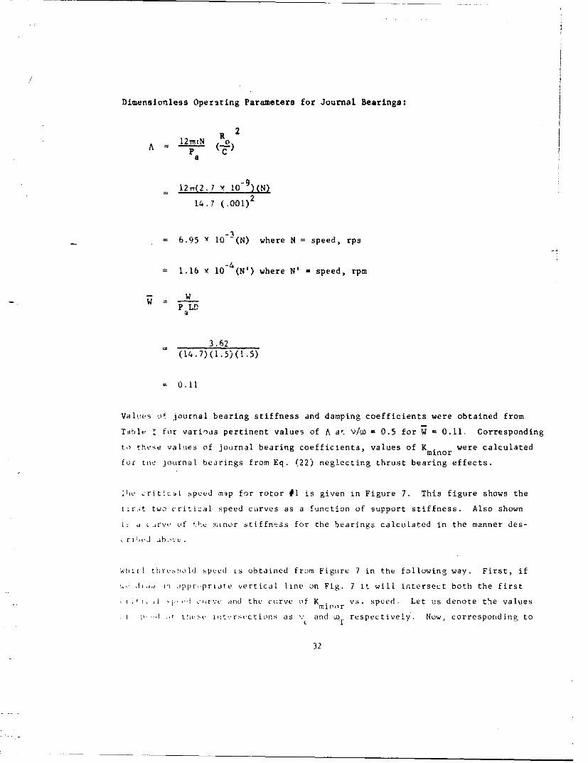
Dimensionless Operating Parameters for Journal Bearings:

A = l2 r N ( _pP c

a

= 12rr(2.1 Y 10- 9)(N)

14.7 (.001)2

= 6.95 Y 10 -(N) where N = speed, rps

1.16 x 10- 4O(N') where N' = speed, rpm

P LD

3.62(14.7)(1-5)(1 .5)

0.11

Valt•es oif journal bearing stiffness and damping coefficients were obtained from

Table T for various pertinent values of A at: v/w = 0.5 for W = 0.11. Corresponding

to these values of journal bearing coefficients, values of K minor were calculated

for tne journal bearings from Eq. (22) neglecting thrust bearing effects.

The critc-:iI speed map for rotor #1 is given in Figure 7. This figure shows the

t~r.it two critical speed curves as a function of support stiffness. Also shown

d, . irve of 0,e minor stiffness for the bearings calculated in the manner des-

,r rl,•J abv.

7hirI thr.sho d sp:eed is obtained from Figure 7 in the following way. First, if

, a, , ,l i, oppripriate vertical line on Fig. 7 it will intersect both the first

i •i, ,1 j i,,,,,i •i;rVL' cmd the curve of K r vs. speed. Let us denote the values

I . t' L,;Lt'v i, t rs ct ions as v and u) respectively. Now, corresponding to

32

LAID

0-0

00

I-j

C-). LL

S-0

-~-c0

UIJ

M C)) 0I

L4Ajj .CIC - -

cr..

Mc coI-.I= L

UI-

LU -

'-4 LUj

IF-

cn 40D'-'C

WdU N 033dS IVOiijO

33

these values of v, the naturn! frequency of oscillation and aT' the rotor speed

at which K is calculated, there will be some value of'whirl frequency ratiominor

Y - v/w calculable from Eq. (14). If this calculated value of Y is exactly equal

to v /W-, then we have determined the whirl threshold condition and u will be ourc

whirl threshold speed while v c T will be our whirl frequency ratio. If, say,

Vc1wT should prove to be less than our calculated value of V, then we must try

drawing another vertical line slightly further to the right and redetermine Vco /T.

If V c/w is less than the value of Y calculated from Eq. (14) then our new ver-

tical line should be drawn slightly further to the left. Usually Y ' 0.5 so we

would first try drawing a vertical line such that vc/aT = 0.5.

In the example shown, neglecting thrust bearing effects, the whirl threshold speed

is found to be A= 3300 rpm while the critical whirl frequency ratio is Y -

0.457.

It should be noted that in using this critical speed mar approach, the curve of

Kminor was calculated for the condition V/I - 0.5 rather than for the condition

v/i = 0.457. For greater accuracy, one could recalculate Kminor at the predicted

critical whirl ratio ef 0.457 and redetermine the whirl threshold. Usually, how-

ever, this would result in only a very small change in the value of threshold

speed and is not necessary.

Next let us consider how we would determine the threshold speed of rotor No. 1 in

a more precise manner using the computer program PN400. In using the program, we

c*n take advantage of the fact that we have already determined the threshold speed

in an approximate manner by the critical speed map approach as described above.

Thtcrefore, with the computer program, we look for the roots of the real and imag-

inary part- of Eq. (10) in the victnity of n = 3300 rpm and Y = 0.457.

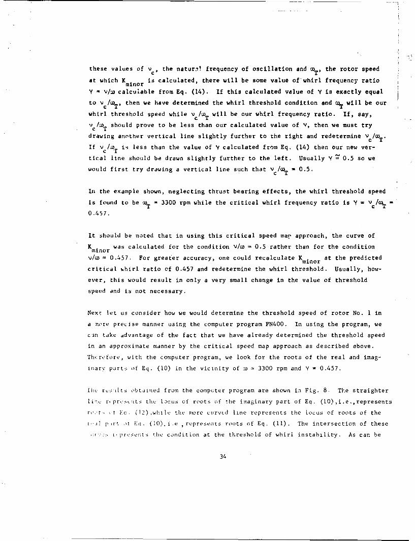
lhu rL:;ilts obtained from the computer program are shown in Fig. 8. The straighter

lic: rtprestzits thu locus of roots of the imaginary part of Eq. (10),i.e.,represents

r- t' ý,t Lo (t2) ,whiIt, the more curvtd line represents the locus of roots of the

. ,t ,,t "I . (10), i.e , represenits roots of Eq. (11). The intersection of these

v u pru :ts the condition at the threshold of whirl instability. As car. be

34

01

0c Iu.I J LLJ 4)

0LJ L/A Lai

0. 1 j 1 49-

00 U 0 LLO - - -J LA

CD ) =- i I--. I(4'

000

V" W) 0 (A LL

Owl I- 0

CL 0l. -

C3 c

4:i

LAS

-J-

S 0

co

LnL

- -

OUV~lAMMOM IN4R

35U

seen, this occurs at a running speed of approximately 3570 rpm and at a frequi

ratio of Y = 0.460.

For comparison, the whirl threshold solution obtained by the approximate critispeed map approach is also shown in Fig. 8. Agreement with the more precise C

puter solution is quite reasonable.

We can now proceed to investigate what change in the calculated value of whirl

threshold speed for our example rotor No. I will result if we consider the thr

bearing angular stiffness and damping in our calculations. The thrust bearing

for this rotor are hydrostatic with dimensions listed on page 25. In the case

hydrostatic thrust bearings, stiffness is the only bearing characteristic one

usually needs consider in determining the influence of the thrust bearing on c

ical mode of whirl instability. This is so for the following reasons:

* (1) Damping, being the result of hydrodynamic forces rather than hydrosta

forces, is a very much weaker force in externally pressurized bearings

than is the stiffness.

(2) The "effective" angular damping in hydrostatic thrust bearings tends

zero at Y Z 0.5 much the same as does the effective radial damping in

plain cylindrical journal bearings. Hence, for whirl frequency ratic

near 0.5, hydrostatic thrust bearing damping will be quite ineffectiv

in increasing the threshold speed for conical whirl instability.

To determine the effects of the hydrostatic thrust bearing stiffness on our ca

culated value of whirl threshold speed, we will first do a rough calculation C

the critical speed map approach and then do a refined calculation using compat

progr;m PN400. Data for the angular stiffness of hydrostatic thrust bearings

given in Figs. 13 through 16 in the next section as a function of the dimensic

feeding parameter A As discussed in the next section, this data is for stat

or stcidy state displacement of the bearing. However, in most cases this is S

plicable to dynamic displacement of the bearing if the frequency v of dynamic

nOcillation is low enough. To determine if steady state data is applicable,

36

calculate the dimensionless squeeze number a

R 0 R io_P a C2

12(2•.7 x 10") v (.333)

14.7(.0011)2

- .605 X 10"V

At

Nt a 3570 rpm

-• - 373 red/sec

! ~~v = - /)

- 187 rad/sec

Therefore

a =.114

From Fig. 18, we see that squeeze number of a 0.114 is sufficiently low such

that steady state values for bearing stiffness apply (see discussion of Figs. 17

and !8 in the next section).

To determine the angular stiffness G from Fig. 16, we must determine the dimension-less feeding parameter A . Our approach is to set A at the value yielding maximum

5 -5

stiffnesi i.e.,A = 1.0 .(This optimum value *for A can be achieved for our bearing,, 2

by the proper choice of na2 in A .) The maximum value of dimensionless angular5

stiffness G Is

37

__+__2 --

G .121 + 2/3 6 2

Now, our bearing is inherently compensated, so S - a2 /cd is sufficiently large

(d 2a and c << a) that the fa..tor

0+ 62 (See References 7 and 8)(1 + 2/3 62)

as 6- a becomes approximately

1+ 3

I 2 22 3

Solving for G from the expression given on Fig. 16 we have

(' 1 + 8 2, G' r (Ro02 R Ri2) Ro"2 (P P )I1 + 2 62(l+6\+1 2 2 2

C 3 + 52

1 + 2/3 8

12 T .(,)2 33)2) (1)2 (73ý5 - 14.7)

(3/2)( 00110)

1 15 x 10 in.l/radian

As descri--ed ýarlier, this angular stiffness may be converted to an effective

i7cri'nt 'n jo'urnal baring stiffness AK which can be added to the existinge

]o,.rrl 5'•.-arin• stiff.i"ss for purposEs of determining whirl tnreshold speed

38

1-2

. 1.15 x 104

(1)2

- 1.15 x 104 lb/in.

For a hydrostatic thrust bearing, the cross-coupling terms are zero and the stiff-

ness in the two principal planes are identical. Since Kmnor is increased directly

by increases in Xxx and K yy, the equivalent increase in stiffness 4K e may be added

directly to the Kinor obtained previously and the resultant curve for Kminor is

plotted in Fig. 7. Using our graphical approach for determining whirl threshold

speed, i.e.,vc/•T must equal y calculated from Eq. (14), we find that the threshold

speed with thrust bearings turns out to be at approximately 6900 rpm. Bearing

stiffness and damping coefficients were therefore obtained for the: hydrodynamic

Jouinal bearing at this value with W - 0.11 using the v/w = 0.50 data. The journal

bearing coefficients were then submitted along with the actual angular thrust bear-

ing coefficients into the computer progran. The results are shown plotted in Fig.

9 which yields a threshold speed of 7170 rpm at v/w - 0.477.

Rotor model No. 1 is an idealized model which serves as an example 'alculation of

how thrust bearing stiffness may significantly improve the stability of the rotor

to fractional frequency conical whirl instability, and how this improvement may be

calculated. In rotor model No. 2 we have an example of an actual prospective de-

sign for a high temperature turbocompressor which was rejected on the basis of its

poor stability characteristics. A simplified drawing of the rotor is shown in

Fig. 6 and a brief description of the rotor was given earlier in this section. Due

to the overhung nature of the design, the lowest mode of fractional frequency

whirl instability was conical in nature. However, since the analytical tools were

not available at the time this design was proposed, no account was taken of the

effect of the thrust bearing in possibly enhancing the rotor stability. We shall

examine the stabilizing influence of this thrust bearing in what follows below.

39

i.

ul 4

LaI LjJ LAJ

w( L) La

0) a- W -j0C3 =fl LL O =

uj CD4-

1= 0

Ltto

0 A 00 0WCDC

-A =IV4ANn~d hH

C)40

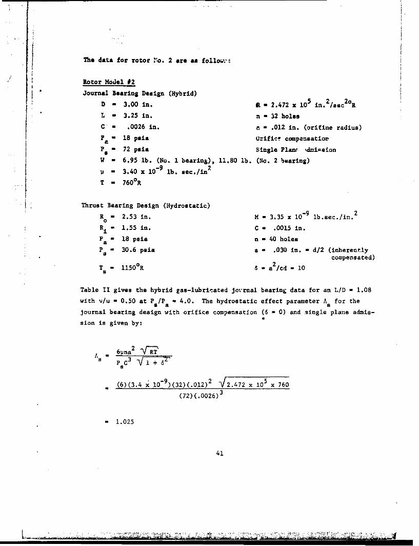
The data for rotor !!o. 2 are as folloý-t

Rotor Model #2

Journal Bearing Design (Hybrid)

D - 3.00 in. t - 2.472 x 105 in.2/sac2R

L - 3.25 in. n - 32 holes

C- .0026 in. a - .012 in. (orifine radius)

P - 18 psia Orifice compensation

Ps 72 psia Single P1an, kdmission

W - 6.95 lb. (No. 1 bearing). 11.80 lb. (No. 2 bearing)

- 3.40 x 10-9 lb. sec./in2

T - 760 0R

Thrust Bearing Design (Hydrostatic)

R - 2.53 in. M - 3.35 x 10-9 lb.sec./in.20

Ri - 1.55 in. C - .0015 in.

Pa - 18 psia n - 40 holes

P M 30.6 psia a - .030 in. - d/2 (inherentlycompensated)

T - 1150 0 R 5 - a 2 /cd - 10

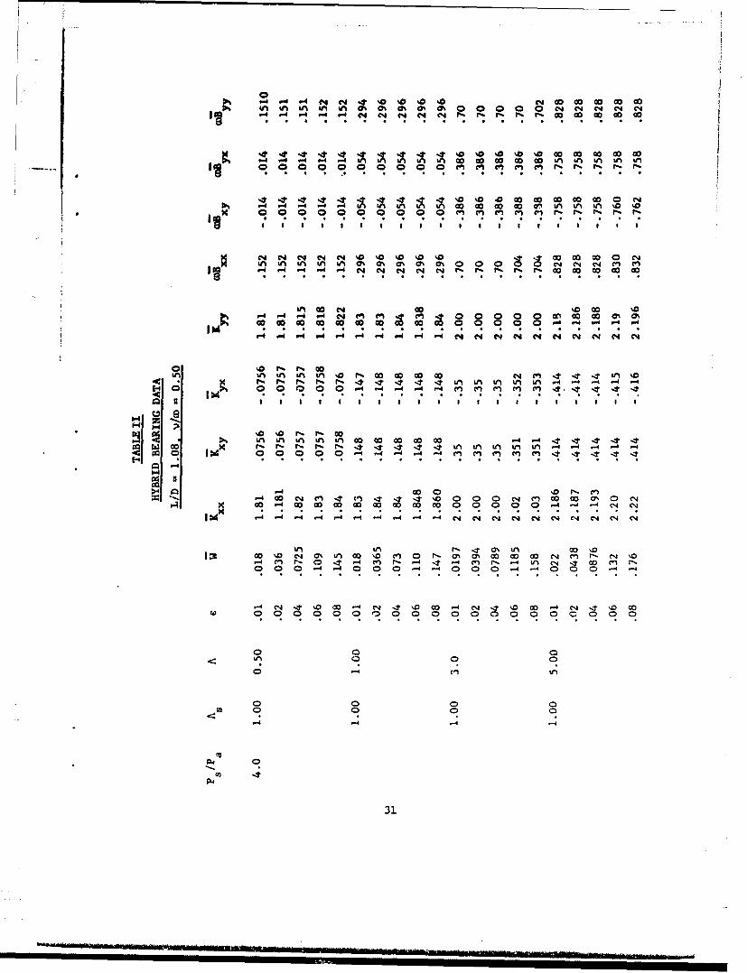
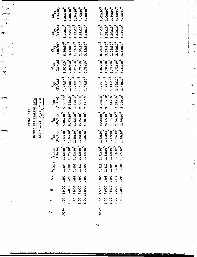
Table II gives the hybrid gas-lubricated journal bearing data for an L/D - 1.08

with v/w - 0.50 at P /P a 4.0. The hydrostatic effect parameter A for the

journal bearing design with orifice compensation (6 - 0) and single plane admis-i

sion is given by:

A 61ina 2 -FTAs "P aC3 "•/ i + 62"

-9 2 52(6)(3.4 x 10 )(32)(.012) 2.472 x 105 x 760

(72)(.0026)3

1.025

41

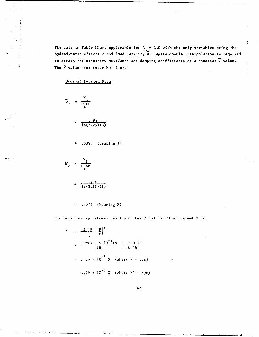
rhe data in Table Hare applicable foi A = 1.0 with the only variables being the

hydrodynamic effects A end load capacity W. Again double interpolation is required

to obtain the necessary stifZness and damping coefficients at a constant W value.

The W values for rotor No. 2 are

Journal Bearing Data

W1= 1 P L-

a

6.9518(3.25) (3)

.0396 (bearing )

W 2W2 PL'

a

11.818(3.25) (3)

- .0672 (bearing 2)

The relation•ihp between bearing nomber A and rotational speed N is:

12 ---, N I R 2

12-(3 1ýx 10 )N 1.500 12

18 .00261

-32 38 10 3 N (where N = rps)

3.9b 10 N' (where N' = rpm)

42

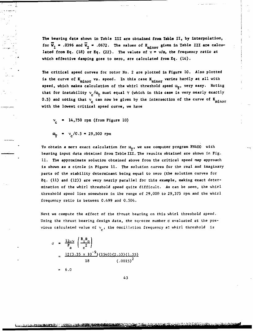
The bearing data shown in Table III are obtained from Table I1, by interpolation,

Vfor - .0396 and W .0672. The values of K given in Table III are calcu-1 2 minor

lated from Eq. (18) or Eq. (22). The values of y - v/m, the frequency ratio at

which effective damping goes to zero, are calculated from Eq. (14).

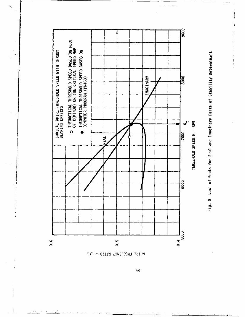
The critical speed curves for rotor No. 2 are plotted in Figure 10. Also plotted

is the curve of Kinor vs. speed. In this case Kminor varies hardly at all with

speed, which makes calculation of the whirl threshold speed PT, very easy. Noting

that for instability vc/wcT must equal Y (which in this case is very nearly exactly

0.5) and noting that vc can now be given by the intersection of the curve of Kminor

with the lowest critical speed curve, we have

vc M 14,750 rpm (from Figure 10)

- v c/0.5 - 29,500 rpm

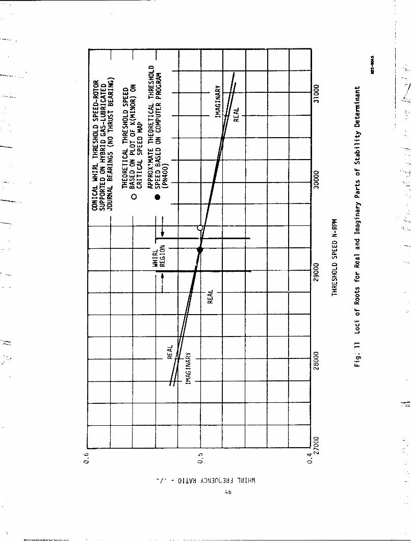
To obtain a mor2 exact calculation for 0T. we use computer program PN400 with

bearing input data obtained from Table III. The results obtained are shown in Fig.

11. The approximate solution obtained above from the critical speed map approach

is shown as a circle in Figure 11. The solution curves for the real and imaginary

parts of the stability determinant being equal to zero (the solution curves for

Eq. (11) and (12)) are very nearly parallel for this example, making exact deter-

mination of the whirl threshold speed quite difficult. As can be seen, the whirl

threshold speed lies somewhere in the range of 29,000 to 29,375 rpm and the whirl

frequency ratio is between 0.499 and 0.504.

Next we compute the effect of the ti-rust bearing on this whirl threshold speed.

Using the thrust bearing design data, the sqeeze number c evaluated at the pre-

vious calculated value of v , the oscillation frequency at whirl threshold isc

1 24v ( RR)

a c

12(3.35 x 10- )(1540)(2.53)(1.55)

18 (.0015)2

- 6.0

43

LaiLUA

V)U

LUJQ Ll-

Q (A

(.-) I

0 C)4

.4- 06

-I-. -C)- '

V)e

LUU

4LU 1____ 0 u.

41ý4

9-4 4 -4P4P44 -4.4 P44-

N .4 N oC4 % C4.c4"A

Pw4 v ~ f -4 N4 -~4 4 P-

1. 4 r- - 14

M.I r4 r-4 4 P- 04 04. 4 4

C91% A~0 . .9 A .4- - .N .0.

0 f . N ILn0 ~ N U

0 0000 0 0 0

1%4 V-4 F-4 t4-4 1%U4 ~ -4 ý 4 "

0-L 00000L 0000ry 4 V-4 F4 "4 pq .4 P4 P4 -4 0.1

3 1 %4 0 0 q VI 0% 0o m% Nq 0 CS~

W.4 N C' 4 4 W r,4 .4 Cý 4 C4

P4V4"4P4"4 4 4 444--

~ 0 N N N in w %a N N4 %D 4

gVn (40 4 C4%4e 0 ~4c4 4

CA 0 0% N U 0% 0 0% .4. 0%

CQ -4 t-4 -- 4 N 4 4 ý4 4 N -N1-4 x 0

14 -4 4 -

0 : c 000 00 00 000aa .4 4.14.4.4.q 4 -1.4.4. ý4..4

V4~~. .0 q00N% C

.0 IT w Q O

I) 0% s-I N 0' m) 0 7% N ON

1-40 Cf,. f ) I) U, if ) C) Cf) 0f_00000 00000

-44 1-

S 0 N Ln N CD" 4 N LN N C.)4

.45

D.~ = L"L 01

coL .L I.-a.

a; -Z cm- - 4

0 a'ý= = Lu" 0

0" 0. --

CMD.0

~~~~A to U~- ~

LW

4.-)

u_ 00

LLEJ

000

CLi.

''-OIIVýI ADN~flG~dJ 1IdIHM

46

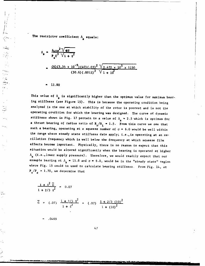
The restrictor coefficient A equals:

, A- 6tna a

(6)(3.35 X 109)(40)(.03)2 V 2 . 4 7 2 10 5 x 1150

(30.6)(.001s)3 V 1 +

. 11.80

This value of A is significantly higher than the optimum value for maximum bear-,aing stiffness (see Figure i5). This is because the operating condition beinganalyzed is the one at which stability of the rotor is poorest and is not theoperating condition for which the bearing was designed. The curve of dynamicstiffness shown in Fig. 17 pertain to a value of A. = 2.5 which is optimum fora thrust bearing of radius ratio of R /Ri M 1.5. From this curve we see thatsuch a bearing, operating at a squeeze number of a = 6.0 would be well within

the range where steady state stiffness data apply; i.e.,is operating at an os-cillation frequency which is well below the frequency at which squeeze filmeffects become important. Physically, there is no reason to expect that thissituation would be altered significantly when the bearing is operated at higherA (i.e.,lower supply pressure). Therefore, we would readily expect that ourexample bearing at As = 11.8 and a = 6.0, would be in the "steady state" regionwhere Fig. 15 could be used to calculate bearing stiffness. From Fig. 14, at

Ts /P a= 1.70, we determine that

+6 G 2- 0.07

1 + 2/3 82

C. =-(.07) = (.07) 1 + 2/3 (10)2

1 + 62 1 + (10)2

= .0469

47

G (R 02_ R 2) Ro2 (Ps" P)

--[(2.53) - (1.55)21 (2.53)2 (30.6 - 18)(.0469).0015

3.02 x 104 in.lb/rad.

Since we have only one thrust bearing, we must appropriately divide its effect

among the two journal bearings to use the effective stiffness - critical speed

map approach for approximately calculating the effect of the thrus-t bearing on

whirl threshold speed. The distance of journal bearings I and 2 rroý., the c.g.

of the rotor are L = 4.72" and L = 2.78" respectively. By analogy with Eq.1 2

(29), which gives the relationships for adding an effective stiffness of one

thrust bearing to on, journal bearing, we can infer that a correct approach for

,dding an effective stiffness of one thrust bearing ot angular stiffness G to

two journal bearings of spans L1 and L2 would be by the relationship

GK 2 2

L1 + L2

Therefore, the effective radial stiffness to be added to each journal bearing

w<)ol Id be

Ge LI + L 2

k2 2

3.02 v 104

30

1010 lb/in

48

This value is seen to be negligible compared with the values of stiffness

associated with the journal bearings themselves. Hence, in this case, the

thrust bearing would have negligible effect on conical motions of the shaft.

The above conclusion reached for rotor No. 2 probably pertains to most rotor

designs. In general, such rotors will be designed so that the span between

journal bearings is efficiently great that these bearings will exert a much

greater restraining force on conical motions of the shaft than will the thrust

bearings. However, this need not always be true. It is easy to conceive of

systems where the thrust loads dominate and where journal bearings are needed

only to locate the shaft. In such systems a designer could take advantage of

the now available technology for including thrust bearing effects in whirl

threshold speed calculations, and design the rotor such that the thrust bear-

ing could assume the responsibility of restraining conical motions of the rotor.

49

SECTION IV

ANCULAR STIFFNESS COEFFICIENTS FOR HYDROSTATIC THRUST BEARINGS

The hydro-.tattc bearing data presented in this section are bssed on an analysis

hy Lund de,cribed in Reference [5]. Basically, the analysis involves the assump-

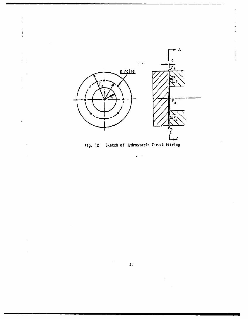
tion that. dii~rete feeding holes arranged in an annular thrust bearing (see FPg.

12) can be represented approximately by a continuous "line bource" of feeding as

if the bearing were fed by a continuous circular slot rather than by discrete

tles. Fhis approximation tends to be absolutely correct in the limit as the

ni:mner of feeding hole, approaches an infinite number, but tends to somewhat over-

estimate bearing load and stiffness for bearings having a finite number of holes.

A line scurce correction factor to account foe this overestimation has been worked

out by comparing a detailed discrete feeding analysis with the simpler line source

analysis Ihe correction factor to be applied depends on the product nr and d/TD

where n is the number of feeding holes, 1/2 log e(R o/Ri), d is the diameter of

tie feeding holes, D = 2 'IRoR • R and R are the outer and inner radii of the

thrust bearings having a practical number of holes, the correction factor to be

applied i• 2/3,i.e., the line source analysis overestimates the stiffness by 50%.

Thi. correctLion factor has been built into the design curves presented in this

sectior. Figure 19 shows a curve of nO vs. d/OD giving the recommended size and

,ikiniber of feedings for which this correction applies. If more feeding holes are

.- ,cl, ýtiffness will be higher than that predicted by the design charts in this

i-ttlkr -nd -onversely.

fDit: stiffn--ýs of compressible hydrostatic bearings is dependent upon the frequency

,)t *xcitati..n v of the bearing if this frequency is high enough. This is because,

-i jrt e val~tei of %, the gas in the bearing film tends to be dropped and cola-

prcs-cd rather than squeezed out of the film. and this corptibutes to a higher

l.I of r -b r aring stiffness. This effect is illuIs;trated in figures 17 and 18 wheredi,,'Is~tlt• s lf neqs•- 2 R 2) 2pa

.tiffness G = CG/ir(R - R. ) R (P - ] is plotted vs. theS0 1 0 S '

Ji',eu.-•ifnlu5 exc itation frequency a (known as squeeze number)

R R

P 2I C

50

A~

Fig. 12 Sketch of Hydrostatic Thrust Bearing

51

as can be seen, for small a, the stiffness remains constant at its steady state

value independent of excitation frequency. However, once v becomes large enough,

the bearing stiffness begins to increase with v due to the above mentioned squeeze

fitm effect.

In general, for rotors supported on hydrostatic bearings, the running speed will

be in the range such that an excitation frequency v .•'/2 will lead to squeeze

nu.mbers sufficiently low such that steady state bearing stiffness data will apply.

This i. generally so because if shaft speeds are high enough such that compress-

ibility becomes significant in the squeeze film effect, then the shaft speed will

tend to be high enough such that hydrodynamic bearings could be used for load

support. Figures 17 and 18 will be used, therefore, primarily to define the lim-

it,i below which steady state bearing data apply rather than being used as a source

of dynamic stiffness data.

In Figures 13 through 16 are nresented dimensionless angular stiffness Z vs. the

feeding parameter A5

A - 6na 2 (31)P pc Vi+T2

s

iar radius ratios of R /R. = 1.25, 1.5, 2,0, and 3.0. The dimensionless stiffness

G 1b pre-,Pultiplied by the factor 1 + 6 2/(1 + 2/3 82) where 5 = a 2cd, known as the2

inherent compensation factor, gives the ratio of orifice area Ta to inherent re-

-striction area icd (see Figure 12). Curves are provided foi different values of

pressure ratio P /P . Usually, the hydrostatic thrust bearings are designed for

a value of A which provides near maximum stiffness; i.e., A is in t'Ae range 1.0

to 4 0, depending on radius ratio. Hence, the dynamic curves in Figs. 17 and 18

arc presented for near optimum values of A •5

Only stiffnet ss data is provided for the hydrostatic bearings. This is for the

following rodaýofs:

52

(1) Damping in hydrostatic bearings results, essentially, from hydrodynamic

forces which are usually much weaker-than the hydrostatic forces produc-

ing bearing stiffness.

(2) Mire importantly, in hydrostatic thrust bearin&s, "effective" bearing

damping tends to zero for wobbling or nutating modes of motion which

occur at half the rotational speed of the thrust runner. In examining

the stability of rotors, it is invariably the influence of precisely

this kind of thrust bearing motion on rotor dynamics that we are at-

tempting to calculate. Hence in such calculations, it is quite reason-

able to presume that the effects of thrust bearing damping will be zero

or near zero and only consider the effects of thrust bearing stiffness.

53

4-

4.

&A 0CL (U

4.-

S- V)

U~ca to (

_ _ _n 0_ (

-1 -. __ ~ 7o-_ _ _l _ _ _ _ AL (

LOA

CO + +

a)

'4-

44

_ _O SO

-/ +_ --- +_. I~

+ L..+ I

55c

0

CLL

U -

-- rII

4-1cma

LA

C, LA1

4-4

Ca. ,.. .D. .

I I In

'jr,

__3 -4 Co

+I

-~M IA

I.-

0o0

cc :C) Ln a 1

CIJ C

- *~ 4E

__ _ dU)o(b b), C/

57jU

I -IA

CLa

'4-)

0 S-

o CL

4 E

-•

-- LI~4-,

- 0- .

Cr4 - a)

oI.. "

"- I

O II- E

---- , --

A

:, :3LL

CI

-F-u

oA 0

4- r

(U

4-3

0..

C~C

-d Sd-8 - - - 0 C

59 00

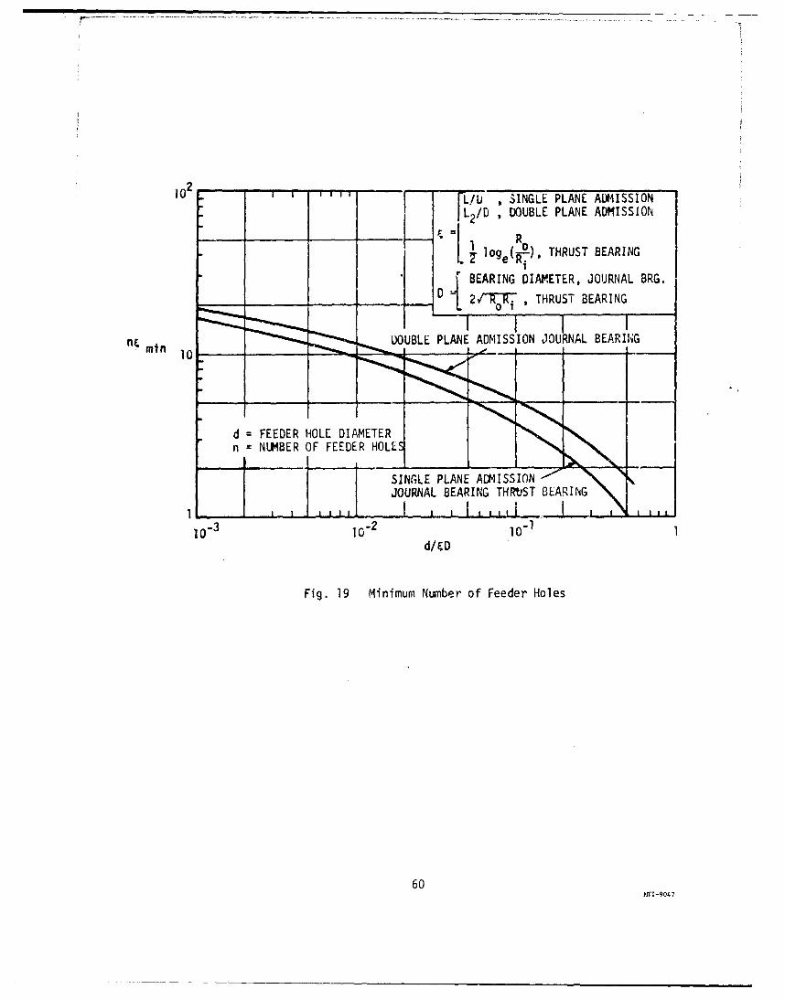
0 L/U SINGLE PLANE ADMISSION

". JL2 /D , DOUBLE PLANE ADMISSION

=[ 1_ _oge(Rii), THRUST BEARING

" BEARING DIAMETER, JOURNAL BRG.

D____ _- L 2 , THRUST BEARING

nc mn DOUBLE PLANE ADMISSION JOURNAL BEARIING

d = FEEDER HOLE DIAMETER

n = NUMBER OF FEEDER HOLLE

SINGLE PLANE ADMISSIONJOURNAL BEARING THRbST BEARING

1o-3 10-2 1o0-d/&D

Fig. 19 Minimura Number of Feeder Holes

60?I'I-9047

APPENDIX I

COHPUTER PIWOGPAM

THE THRESHOLD OF INSTABILITY OF 'A FLEXIBLE ROTOR IN FLUID FILM BEARINGS

This section describes the rotor stability computer program PN400: "The Threshold

of Instability of a Flexible Rotor in Fluid Film Bearings". This program is quite

similar to the computer program PNO017 given irn Reference 1.

The new program described in this volume is a modification and extension of the

previous versior. The amount of plotting has been significantly reduced in that

a quadratic interpolationI routine now automatically performs much of the plotting

previously required to find the zero point solutions for both the real and imagin-

ary parts of the complex determinant. This program also rnw accepts the angular

thrust bearing properties and is also set up to handle both liquid-lubricated and

gas-lubricated bearings. In addition a more refined rotor model is employed which

describes the rotor in terms of stiffness and mass diameters, lengths, concen-

trated values of mass, and mass moments of inertia. The new rotor model is dis-

cussed in Reference 3.

Analysis

The rotor analysis is described in detail in Reference 3, Appendix VIIL. Con-

sider the rotor shown in Fig. 3 and assuming the two ends of the rotor to be

free, the bending moment and the shear force at one rotor end are directly pro-

portional to the unknown amplitude and slope at the opposite rotor ond. The

proportionality coefficients are the dynamic influence coefficients which are

computed by the program, cnd the final equation is given in the.following matrix

form (see Eq. (H.61) in Appendix VIII of Reference 3 neglecting magneti: influence

coefficient matrix).

Second-order polynomial interpolation. See Reference 6.

61

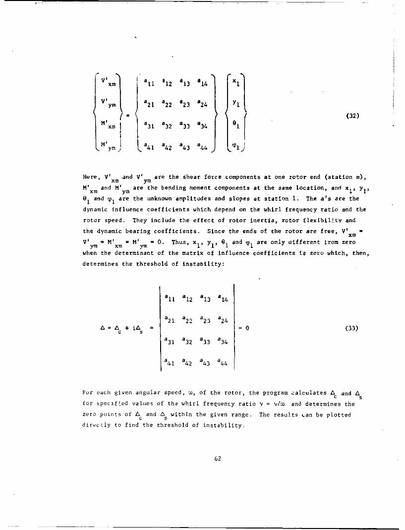
xm 1 12 13 14

VIym a21 a22 a23 :24 Yl

8xm a 31 a 3 2 a33 a 3 4 9 1 (32)

t ymI a4 1 a 4 2 a43 a 4 4 CI)

Here, V' and V' are the shear force components at one rotor end (station m),xm ym

M'xm and M'ym are the bending moment components at the same location, and xI, Yl,

0 and rp are the unknown amplitudes and slopes at station 1. The a's are the

dynamic influence coefficients which depend on the whirl frequency ratio and the

rotor speed. They include the effect of rotor inertia, rotor flexibility and

the dynamic bearing coefficients. Since the ends of the rotor are free, V'xm

V'ym = M'xm = M'ym = 0. Thus, xI, YI, e1 and cpl are only different from zero

when the determinant of the matrix of influence coefficients is zero which, then,

determines the threshold of instability:

a11 a12 a13 a14

a21 a22 a23 a24

&= + i =0 (33)c s

a31 a32 a33 a34

a41 a42 a43 a44

For each given angular speed, w, of the rotor, the program calculates & andc S

for specified values of the whirl frequency ratio y = v/w and determines the

zero points of L and I within the given range. The results can be plottedc S

directly to find the threshold of instability.

62

COMPUTER INPUT

Card 1 (72H)

Any descriptive text may be given to identify the calculation.

Card 2 (1415)

This is the "control card" whose values control the rest of the iinput. The con-

trol card has 10 items:

1. NS, the number of rotor stations, see "Rotor Data" (1 < NS < 100)

2. NB, the number of bearings (I < NB < 10)

3. NPST. The program provides for including the response characteristics of

the bearing pedestals. When it is desired to include this effect, set NPST

and give the required input data as explained later. When NPST = 0, the pedes-

tals are assumed to be rigid and no pedestal data are required in the input.

4. HANG. The dynamic forces of the fluid film in the journal bearings resist

both radial motion and angular motion. In most cases, only the radial forces

are significant in which case NANG is set equal to zero. However, long jour-

nal bearings and especially thrust bearings may exert considerable constraint

on the angular motion of the rotor. When it is desired to include this effect,

set HANG = I and give the required input data as explained later.

5. NFR is the number of whirl frequency ratios specified in the input list

below, see explanation later (3 < NFR < 50).

6. INC. If the bearing lubricant is compressible (gas bearings), uet INC = 1

in which case the dynamic bearing coefficients must be specified for each whirl

frequency ratio in the input. If INC = 0, the lubricant is incompressible andthe dynamic bearing coefficients are independent of whirl frequency.

63

7. NIT. As discussed previously, the program searches for the zero points

of the instability determinant. To do this, the instability determinant is

computed as a function of the whirl frequency ratio. The input gives NFR

values of the whirl frequency ratio in sequence, and the determinant is cal-

culated for each of these values. In addition, each interval is subdivided

into NIT increments and the determinant is also computed at these intermedi-

ate frequency ratio values. Whenever the program detects a change in sign

of the determinant between two consecutive calculations, it uses quadratic

interpolation to find the accurate zero point.

By subdividing the intervals in the given frequency ratio list, the list can

be shortened without los5 of accuracy. Furthermore, when the bearing lubri-

cant is a gas it is necessary to provide the dynamic coefficients for each

specified frequency ratio. Thus, to minimize the input data it is desirable

to keep this number low. Then the program automatically calculates the coef-

ficients for the intermediate points by quadratic interpolation.

NIT should be eqi.gl to or greater than 1. When NIT - 1, no subdivision takes

place.

8 METR. This item should always be zero. It is included for diagnostic

ptirposes which, however, is of no value to the general user of the program.

9. NCAL, specifies the number of rotor speed ranges. For each speed range

it is necessary to give input data for the dynamic bearing coefficients.

There is no limit for NCAL.

10. INP. If INF = U, the present set of input data is followed by a new set,

itarting from Carl 1. If INP - 1, this is the last set of input.

Cdrd 3 (1F6E12.5)2.I'M is Youngs modulus E for the shaft material in lbs/inch . If E actually

changes along the rotor it should be noted that the program only uses E in the

prod~ict El where I is the cross-sectional mor-ent of inertia of the shaft. Since

64

' 6U C (d) - di where (do0) is the outer shaft diameter and di isstiff stiff

the inner diameter, any variation in E can be accounted for by changing (do)

(see "Rotor Data").

2. DENST gives the weight density of the shaft material in lbs/inch 3. The pro-

gram converts it into the mass density o - DENST/386.069. If the density actually

changes along the rotor it should be noted that the weight of the shaft per unit

length is (d ) - where (do) is the outer shaft diameter (seeL mass Jmass

"Rotor Data"). Thus, (do) can be changed to absorb the changes in density.mass

23. SHM gives the product oG where G is the shear modulus, lbs/inch , and c is

the shape factor for shear (for circul.r croas-sections: o Z 0.75).

Rotor Data (8E9.2)

Thr rotor is represented by a number of stations connected by shaft sections

of uniform diameter. Thus, rotor stations are introduced wherever the shaft

diameter changes (or changes significantly). Also, there must be a rotor sta-

tion at each end of the rotor, at each bearing centerline and at any thrust

bearing. Furthermore, a rotor station is introduced wherever the shaft has a

concentrated mass which cannot readily be represented in terms of an inner and

outer shaft diameter (impellers, turbine wheels, alternator poles, and so on).

In this way the rotor is assigned a total of NS stations (card 2, item 1) which

are numbered consecutively starting from one end of the rotor. There can be a

maximum of 100 stations. Eaci: station can be assigned a concentrated mass m

with a polar mass moment of inertia I and a transverse mass moment of inertiap

IT (any of these quantities may, of course, be zero). Also, each station can

be assigned a shaft section with which it is connected to the following station.

This shaft section has a length L, and outer diameter (d ) stiff, an outer diameter

(d ) and an inner diameter d. . The outer diameter (d ) is used to spec-massstf

ify the stiffness of the shaft sect°on such that the cross-sectional moment of

inertia of the shaft is- I = -- (d )4 - di4] and the shear area is:5 stiff

65

d j~) 2 - d 2 The outer diameter (d ) is used in calculating the4 0o: 1 ] ,

L( stiff m 0 ass

mass of the shaft such th~it the mass per unit length is: 0 (Td)2 - d

where 0 is the mass density (see card 3, item 2). J

In the computer input there must be a card for each rotor station (NS cards).

Each card specifies the 7 values for the stationi:

1. The concentrated mass: m, lbs. (may be zero).

2L Tne polar mass moment of inertia of the station mass; I lbs-inch2 (may bapzero).

3. The transverse mass moment of inertia of the station mass; IT lbs-inch2 (maybe zero).

4. The length of the shaft section to the next station: L, inch (may be z.ero).

For the last station, set I = 0.

5. The outer diameter, (d0) of the shaft section, inch. (do)stiff is usedstiffstf

in calculating the stiffness of the shaft section, (d 0 ) s 0. For the last

station, set (d ) s 1.0.0stiff

b. rhe outer diameter, (do) of the shaft section, inch (may be zero).mass

(d ) is used in calculating the mass of the shaft section. For the lastm J s S

Sration, set (d) = 0.mass

7. The inner diameter, d. of the shaft section, inch (may be zero). d. is used

bioth in calculating the stiffness and the mass of the shaft section. For the

last station, set d. = 0.

6b

Bearing Stations (1415)

The rotor station numbers at which there are bearings, are listed in sequence.

This includes both 4ourn3l bearings and any thrust bearings. There car. be up

to 10 bearings.

Pedestal Data (1P6E12.5)

The program provides for the option that the pedestals supporting the bearings

may be flexible. In that case, data for the pedestals must be given and NPST

must be set equal to 1 (card 2, item 3). If the pedestals are rigid, set NPST

- 0 and omit giving any data for the pedestals.

When NPST a 1, each bearing is supported in a "two-dimensional" pedestal. The

pedestal is represented as two separate masses, each mass on its own spring

and dashpot. The one mass-spring-dashpot system represents the pedestal char-

acteristics in the x-direction, (the vertical direction) and the other system

represents the y-direction (the horizontal direction). There is no coupling

between the two systems. In the computer input there must be one card for

each rotor bearing and each card contains the 6 items necessary to specify the

pedestal characteristics:

I. The pedestal mass for the x-direction, lbs.

2. The pedestal stiffness for the x-direction, lbs/inch.

3. The pedestal damping coefficient for the x-direction, lbs-sec/inch.

(Note: For the bearing films the damping is given in lbs/inch, whereas the

damping coefficient in lbs-sec/inch is used for the pedestals).

.. The pedestal mass for the y-direction, lbs.

5. The pedestal stiffness for the y-direct.on. lbs/inch.

67

6. The pedestal damping coefficient for the y-direction, lbs-sec/inch.

When the bearings also have angular stiffness (i.e., NANG - 1, item 4, card 2)

and the pedestals are flexible (i.e.,rfST = 1), the above NB cards must be

followed by additional NB cards, one f,.r eech bearing, on which are specified

the dynamic model of the pedestals for angular motion. Each card contains six

values :

1. Tile pedestal mass moment of inertia in the x-plane (around the y-axis),2lbs-inch

2. The pede.stal angular stiffness in the x-plane (around the y-axis), lbs.

inch/radian.

3. Dhe pedestal angular damping coefficient in the x-plane (around the y-axis),

lbs-inch-sec/radian.

4 The pedestal mass moment of inertia in the y-plane (around the x-axis)2lbs- inch

5. The pedestal angular stiffness in the y-plane (around the x-axis), lbs.

i nc h/r,3d ian .

b6 The pedestal angular damping coefficient in the y-plane (around the x-axis),

Ibs-inch-sec/radian.

Wh}irl Frequency Ratios (IP6EI2.5)

When tCie rotor becomes unstable it whirls in a closed orbit with an angular

frequency , which normally is equal to approximately one half the rotational

frequency n). However, the exact value depends on the rotor and the supporting

bearings, and to determine this the program searches for the zero points of

the stability determinant. The present input list gives NFR values (card 2,

item 5) in sequence of the whirl frequency ratio \/,o) and these values are used

68

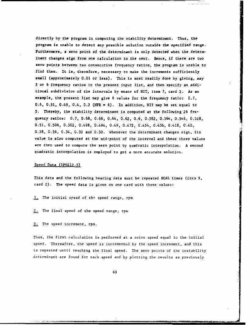
directly by the program in computing the stability determinant. Thus, the

program is unable to detect any possible solution outside the specified range.

Furthermore, a zero point of the determinant is only detected when the determ-

inant changes sign from one calculation to the next. Hence, if there are two

zero points between two consecutive frequency ratios, the progiam is unable to

find them. It is, therefore, necessary to make the increments sufficiently

small (approximately 0.01 or less). This is most readily done by giving, say5 or 6 frequency ratios in the present input list, and then specify an addi-

tional subdivision of the intervals by meant of NIT, item 7, card 2. As an

example, the present list may give 6 values for the frequency ratio: 0.7,

0.6, 0.51, 0.49, 0.4, 0.3 (NFR - 6). In addition, NIT may be set equal to

5. Thereby, the stability determinant is computed at the following 26 fre-

quency ratios: 0.7, 0.68, 0.66, 0.64, 0.62, 0.6, 0.582, 0.564, 0.546, 0.528,

0.51, 0.506, 0.502, 0.498, 0.494, 0.49, 0.472, 0.454, 0.436, 0.418, 0.40,

0.38, 0.36, 0.34, 0.32 and 0.30. Whenever the determinant changes sign, its

value is also computed at the mid-point of the interval and these three values

are then used to compute the zero point by quadratic interpolation. A second

quadratic interpolation is employed to get a more accurate solution.

Speed Data (IP6E12.5)

This data and the following bearing data must be repeated NCAL times (item 9,

card 2). The speed data is given on one card with three values:

1. The initial speed of thi speed range, rpm

2. The final speed of the speed range, rpn,

3. The speed increment, rpm.

Thus, the first calculation is performed at a rotor speed equal to the initial

speed. Thereafter, the speed is incremented by the speed increment, and this

is repeated until reaching the final speed. The zero points of the instability

determinant are found for each speed and by plotting the results as previously

69

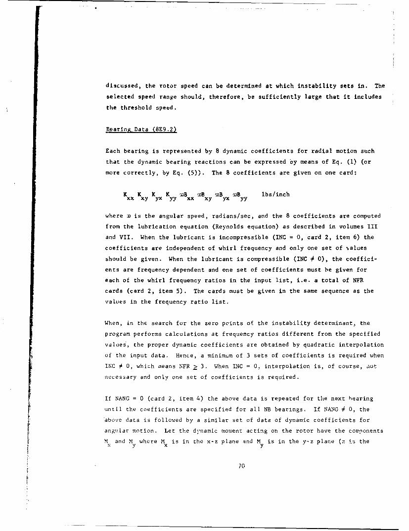
discussed, the rotor speed can be determined at which instability sets in. The

selected speed range should, therefore, be sufficiently large that it includes

the threshold speed.

Bearing Data (8E9.2)

Each bearing is represented by 8 dynamic coefficients for radial motion such

that the dynamic bearing reactions can be expressed by means of Eq. (1) (or

more correctly, by Eq. (5)). The 8 coefficients are given on one card:

K K K K wB wB wB WB lbs/inchxx xy yx yy xx xy yx yy

where j) is the angular speed, radians/sec, and the 8 coefficients are computed

from the lubrication equation (Reynolds equation) as described in volumes III

and VII. When the lubricant is incompressible (INC = 0, card 2, item 6) the

coefficients are independent of whirl frequency and only one set of values

should be given. When the lubricant is compressible (INC 0 0), the coeffici-

ents are frequency dependent and one set of coefficients must he given for

each of the whirl frequency ratios in the input list, i.e. a total of NFR

cards (card 2, item 5). The cards must be given in the same sequence as the

values in the frequency ratio list.

When, in the search for the zero peints of the instability determinant, the

program performs calculations at frequency ratios different from the specified

values, the proper dynamic coefficients are obtained by quadratic interpolation

of the input data. Hence, a minimum of 3 sets of coefficients is required when

INC # 0, which means NFR > 3. When INC = 0, interpolation is, of course, aot

necessary and only one set of coefficients is required.

If NANG = 0 (card 2, item 4) the above data is repeated for the next bearing

until the coefficients are specified for all NB bearings. If NANG # 0, the

above data is followed by a similar set of data of dynamic coefficients for

angular motion. Let the dynamic moment acting on the rotor have the components

M and M where M is in the x-z plane and M is in the y-z plane (z is thex y xy

70

coordinate along the rotor iais). The rotor amplitudes are x and y and the cor-repondina rotor slopes are: B - dx/dz and c = dy/dz. The equations defining

the angular dynamic coefficients are:

G e D d-G % Dx x xi 2t xy y dt

(34)

,do dcoM -G - D - - G c-vd

y yx yx dt yy yy dt

where t is time. These equations are completely analogous to Eq. (1). The 8

coefficients apply to 8 given bearing geometry, a known static bearing load and

are functions of the rotor speed. For compressible lubricPnts, the coefficients

also depend on the whirl frequency ratio such that Eq. (34) more properly should

be written:

M -Y 0 Yx xx xy

(35)

14 = -y Q-Y ¥

y yX yy

where:

+i(-)coD (36)

xx xx t) xx

and similarly for Y, Y and Y Eq. (35) is analogous to Eq. (5) and is de-

rived in the same way..

In the computer input, the B coefficients are given on one card:

C xG G G '.nD ci D oi W lbs.inch/radianGxx xy Gyx yy XX 0•xy yXDyy

In complete analogy to the input for the radial dynamic coefficients, only one

71

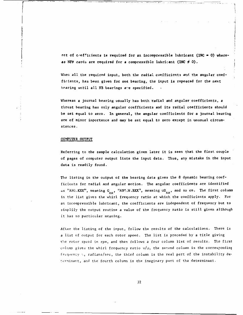
iet of cief•icients is required for an incompressible lubricant (INC 0) where-

as NFV cards are required for a compressible lubricant (INC # 0).

When all the required input, both the radial coefficients and the angular coef-

ficients, has been given for one bearing, the input is repeated for the next

bearing until all NB bearings a'7e specified.

Whereas a journal bearing usually has both radial and angular coefficients, a

thrust bearing has only angular coefficients and its radial coefficients should

be set equal to zero. In general, the angular coefficients for a journal bearing

are of minor importance and may be set equal to zero except in unusual circum-

stances.

COMPUTER OUTPUT

Referring to the sample calculation given later it is seen that the first couple

of pages of computer output lists the input data. Thus, any mistake in the input

data is readily found.

The listing in the output of the bearing data gives the 8 dynamic bearing coef-

ficients for radial and angular motion. The angular coefficients are identified

as "ANG.KXX", meaning Gx "ANr.W.BXX", meaning aoD x, and so on. The first column

in the list gives the whirl frequency ratio at which the coefficients apply. For

an incompressible lubricant, the coefficients are independent of frequency but to

simplify the output routine a value of the frequency ratio is still given although

it has no particular meaning.

After the listing of the input, follow the results of the calculations. There is

a list of output for each rotor speed. The list is preceded by a title giving

t'le rotor speed in rpm, and then follows a four column list of results. The first

column gives the whirl frequency ratio v/n, the se':ond column is the correspondinj

freq'lcncy '., radians/sec, the third column is the real part of the instability de-

ter•l•nant, and the fourth column is the imaginary part of the determinant.

72

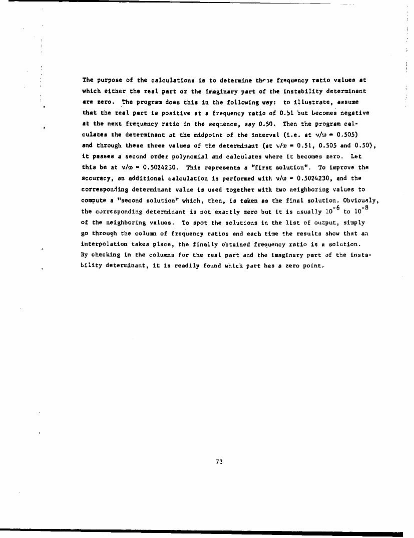
The purpose of the calculations is to determine thrie frequency ratio values at

which either the real part or the imaginary part of the instability determinant

are zero. The program does this in the following way: to illustrate, assume

that the real part is positive at a frequency ratio of 0.51 but becomes negative

at the next frequency ratio in the seqaence, say 0.50. Then the program cal-

culates the determinant at the midpoint of the interval (i.e. at v/h - 0.505)

and through these three values of the determinant (at v// - 0.51, 0.505 and 0.50),

it passes a second order polynomial and calculates where it becomes zero. Let

this be at v/w - 0.5024230. This represents a "first solution". To improve the

accuracy, an additional calculation is performed with v/o - 0.5024230, and the

corresponding determinant value is used together with two neighboring values to

compute a "second solution" which, then, is taken as the final solution. Obviously,

the corresponding determinant is not exactly zero but it is usually 10-6 to 10"8

of the neighboring values. To spot the solutions in the list of output, simply

go through the column of frequency ratios and each time the results show that an

interpolation takes place, the finally obtained frequency ratio is a solution.

By checking in the columns for the real part and the imaginary part of the insta-

bility determinant, it is readily found which part has a zero point.

73

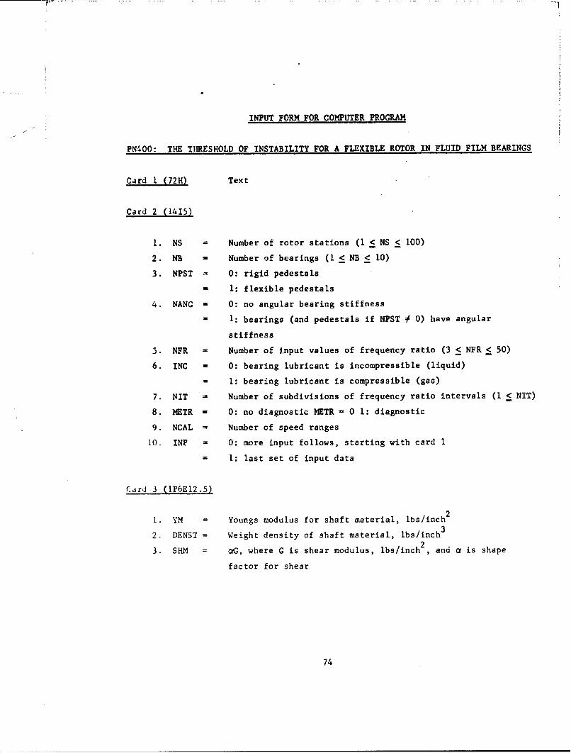
INPUT FORM FOR COMPUTER PROGRAM

PN400: THE THRESHOLD OF INSTABILITY FOR A FLEXIBLE ROTOR IN FLUID FILM BEARINGS

Card 1 (72H) Text

Card 2 (1415)

1. NS = Number of rotor stations (1 < NS < 100)

2. NB Number of bearings (I < NB < 10)

3. NPST 0: rigid pedestals

1: flexible pedestals

4. NANG = 0: no angular bearing stiffness

- 1: bearings (and pedestals if NPST 0 0) have angular

stiffness

5. NFR - Number of input values of frequency ratio (3 < NFR < 50)

6. INC - 0: bearing lubricant is incompressible (liquid)

= I: bearing lubricant is compressible (gas)

7. NIT = Number of subdivisions of frequency ratio intervals (I < NIT)

8. METR = 0: no diagnostic HETR - 0 1: diagnostic

9. NCAL - Number of speed ranges

10. INP = 0: more input follows, starting with card I

= I: last set of input data

Card 3 (IP6EI2.5)

1. YM = Youngs modulus for shaft material, lbs/inch2

2. DENST = Weight density of shaft material, lbs/inch3

23. SHM = oG, where G is shear modulus, lbs/inch , and c is shape

factor for shear

74

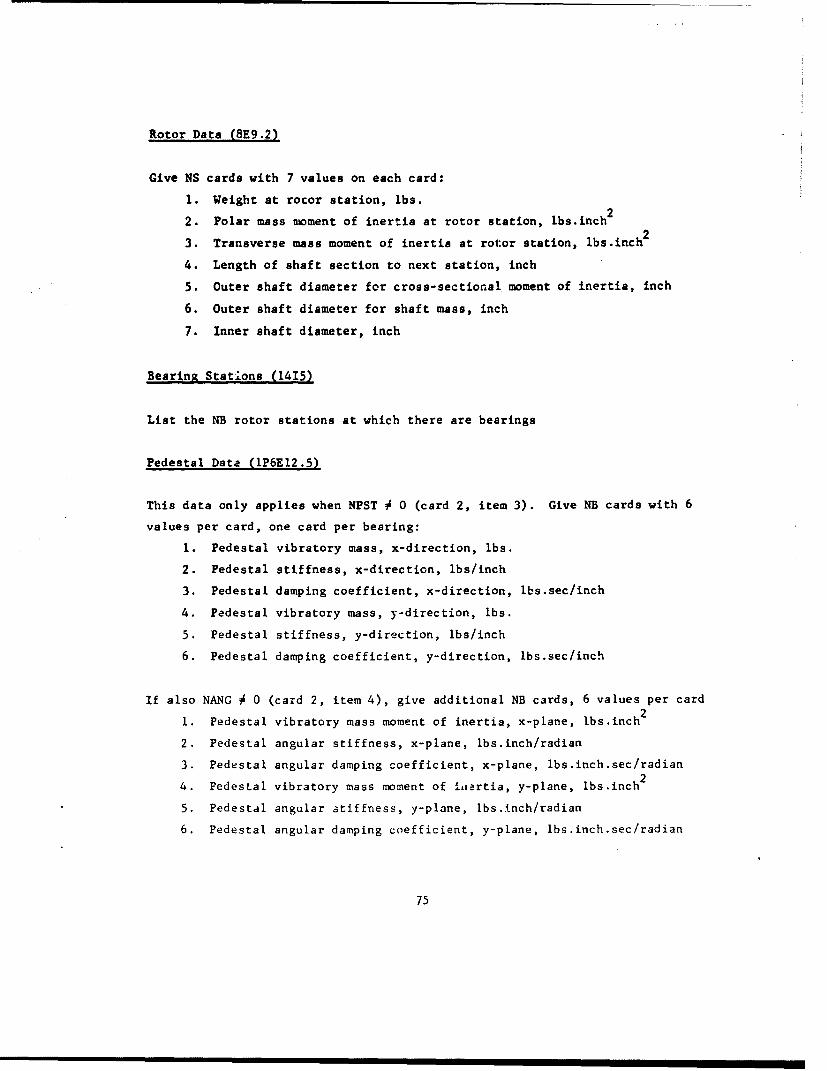
Rotor Data (8E9.2)

Give NS cards with 7 values on each card:

1. Weight at rotor station, lbs.

2. Polar mass moment of inertia at rotor station, lbs.inch2

3. Transverse mass moment of inertia at rotor station, lbs.inch2

4. Length of shaft section to next station, inch

5. Outer shaft diameter for cross-sectional moment of inertia, inch

6. Outer shaft diameter for shaft mass, inch

7. Inner shaft diameter, inch

Bearing Stations (1415)

List the NB rotor stations at which there are bearings

Pedestal Data (IP6E12.5)

This data only applies when NPST 0 0 (card 2, item 3). Give NB cards with 6

values per card, one card per bearing:

1. Pedestal vibratory mass, x-direction, lbs.

2. Pedestal stiffness, x-direction, lbs/inch

3. Pedestal damping coefficient, x-direction, lbs.sec/inch

4. Pedestal vibratory mass, y-direction, lbs.

5. Pedestal stiffness, y-direction, lbs/inch

6. Pedestal damping coefficient, y-direction, lbs.sec/inch

If also NANG 0 0 (card 2, item 4), give additional NB cards, 6 values per card

1. Pedestal vibratory mass moment of inertia, x-plane, lbs.inch 2

2. Pedestal angular stiffness, x-plane, lbs.inch/radian

3. Pedestal angular damping coefficient, x-plane, lbs.inch.sec/radian

4. Pedestal vibratory mass moment of 'iLrtia, y-plane, lbs.inch2

5. Pedestal angular stiffness, y-plane, lbs.inch/radian

6. Pedestal angular damping coefficient, y-plane, lbs.inch.sec/radian

75

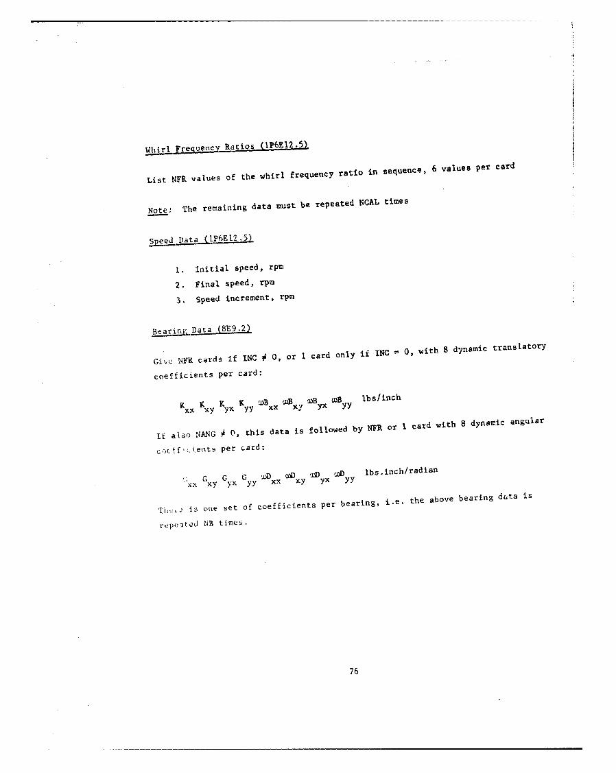
Whirl Frequency Ratios ( AP6El2.5)

List NFR values of the whirl frequency ratio in sequence, 6 values per card

Note: The remaining data must be repeated NCAL times

Speed I)ata (1P6E12.5)

1. Initial speed, rpm

2. Final speed, rpm

3. Speed increment, rpm

BearijELData (8E9.2)

Give NFR cards if INC 0 0, or I card only if INC 0, with 8 dynamic translatory

coefficients per card:

K xx KXY K YX K yy 'Bx y uB yxB •Byy Ilbs/inch

If also NANG 4 0, this data is followed by NFR or I card with 8 dynamic angular

co~fc.ients per card:

GG G G ýDD WD 1D • UD lbs.inch/radian

xx xy yx yy xx xy yX yy

. is one set of coefficients per bearing, i.e. the above bearing data is

r~peited NB times.

76

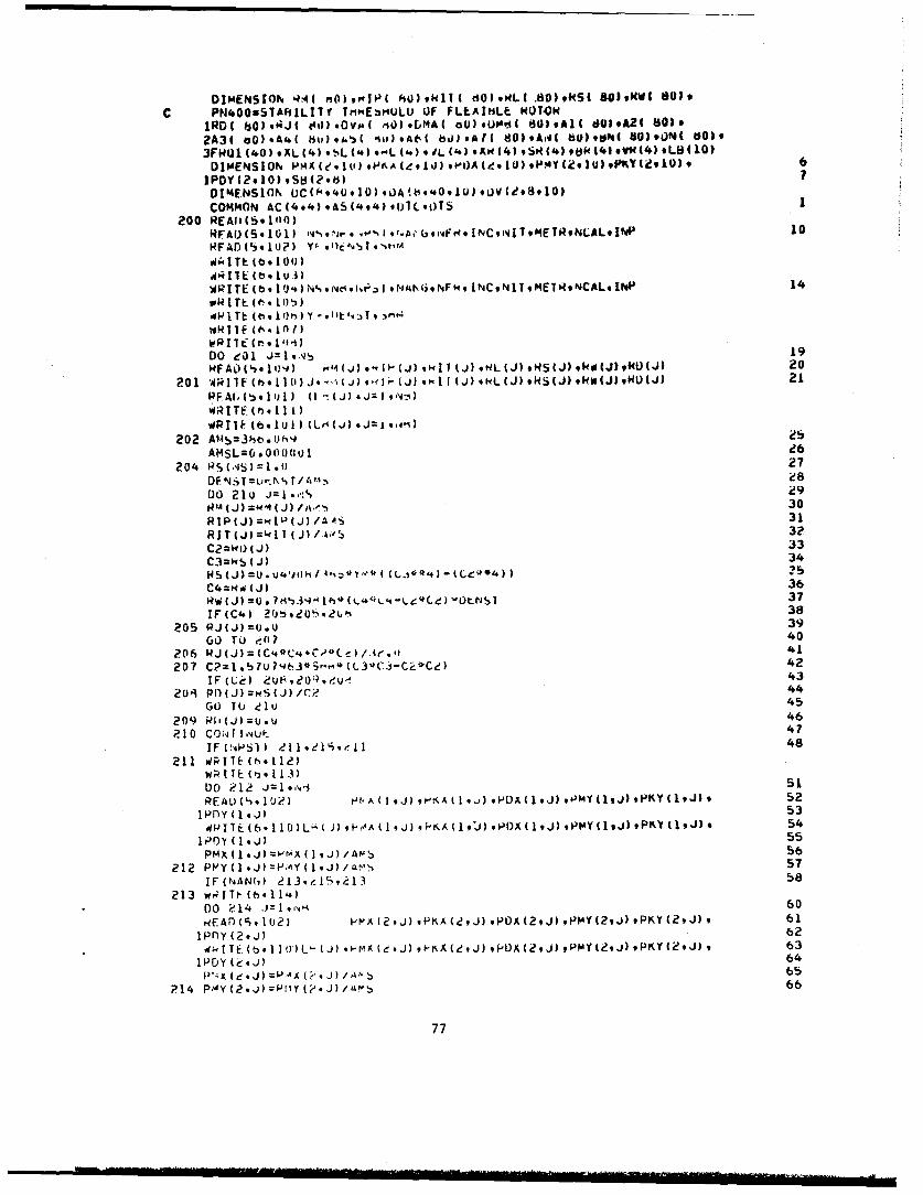
DIMENSION 4A( m0)*mEII( hjU)9HI1( d0I..L( .80)tkS( &03,NW( 80)*C PN400sST*VIILITI TnPCEbMULU OF FLEAI)LE HOTOIR

D ImENS ION PmX4 (e -I to) *OA (e 1 ) .. gA (e 9 0)#PYC2.i91U) *PT (29 10) 9

DIME~NSION VC(As4U.10)9,Obs¶40 " 10,IJV(d98vI0)COMMON AC (4.4) .AS(4v4?,OlCst)Is I

200 REAll (5 104)RFAU(Sol0l) 001 0 N- e W"I 9-A't9 000INC 9d1 T 9ME TRoN(.AL* I% 10

DO ollT (be100)b 1

40 i I 21 t 01uJ

202 I=~U' TE( 20)N%9i5 ~~ A 9N N 79M7R CL W1

ORL&.O~ 1 TE2691 n t -: ~

Dp 1 N (, T 1* ifi) ~2DO) e1u J~lq.'S 19

WF A0 ( 4 *Iiq J ,()91 j L()#S()9kl(J) /AU 3J 0

20 R 1TF(h e 1(1 ) (~' 3)I? J 1()9R J)9R J k )PU()2C2W105) I(J) I33I- J)oJ

WPC IF b U) 341)(r4( = ,m

204 RJ(JA)=U.0 39

00 2ue j2U.,,:% i!9'

20iRf(J)=1411(J)/AC?` 44

209 '(J)U. 46

DO d12 el"?~ 40

206 Y(1J)=C*4C*Cl-e? 41

543

212 P?0Y(1J) ws(J)/(1 44)

Go (NA(, el3v 45~1

210 C214 f lmu e4N46

REafl(Svlu?) I.trAU2,J),PKA(12,J),POAC2,j),PMYC2,iJ)PKY(l9J);- 51

1POD9V 556

213 (e.J I PA (' ((- *) 11- )

214 P4Y(2.J):PI1Y C?.J)/4A'bS 66

77

215 REAWS9b102) (Ftqf1(j);j=19KFR)WRITE (6.1ib)

WHIE=o10,(gs1J.:IdW 70

301 REAb(5.1U2) SPST*SPrP;'..S.~jKjzNFR 72IF(INC) 303*30?93U. 73

302 K1=1 74303 aWITF(69116

DO 310 K:1*44 78WRJTE (6.11IP)L.4(K)wRITE (6.1ll)0O job j=1.K1

306 AJr(,1i)-1()*(.C(..JN.11)IF(NANOj) lUl.310.3iJ? 84

307 ,4w1Tribs12u)00 Joni J=l106l 86

310 CUNTINUE 89SPr,=SPS I 90

320 Wý=.0117~ý1 91

10:14F~..:FP01 MI YhKR=0 96KE=O 97K1=1 98K?=O 99K3=u 100OF-4NI T 101

102325 Fk=ANSPIFwm 103

FR02=F Ntj'F -q104DO 3eb 6 jI !,) 105

DV AI J =Fw~e~'ý,(j)106UL4A(j) =F k~jceI T (j) 107

326 DMP(j) Fk()*ANP*H I r (j) 108330 00 375 J=1s.s 109

IF(INC) 3ld3,e31q.34Se 110331 11=1 III

GO TO 31'. 112

333 I1Ikj 114334. 00 3.,)h 1=1.m~ 115

SW (1q1)= :cC(I * TI j) 116IF (Ni.aNb) jJ - .i j-,j., 117

33~~5i- ~.I~ 11* 11833,S C ON' 1 .uL~ 119

GO 11; J.3, 120339 11=1w 121

I ?=? 12213=0 123JF (N3) 3409340*.p.-iv- 124

339 ll:I'j+1 125340 IF('.4P-11 3L(qL'94 126341 C4=FNOI(11~l) 127

C2C4-;P.1 (I1*1)-' 128

CJ:CI ce 130C4:=F I-W-C'. 131DO 355 1-1l,8 132C5=!)C ( 1.011 9 J) 133

78

Best Available Copy

C7SC6+Cs 136

c63Fc2*c6-CI*Ca 13?

CosC5*C9* (C6*CY*C7) 138

I1711-12) 343o.3429343 139

342 S8(1,1)*C8 140

IVNANG) 34793*35934'7 141

343 IFVIJ) 3449,344.,345 142

344 SRI~,)=C8/C2*(PIWa-FNfj1(11-1)) 143

!F(IANG) )47o3559347 144

IF(NANG) 34793tbS,*J'. 146

347 C5=DA(Itl1.J) 147C6=(A(1I1.,J)-~)/C1~.J)148

C7cC6*Cd ISO

C6=C2*c6-C I C6 151

C8xC5+C9*IC6*C9*Cl ?j 52

IFC11-1e) J'.YJ40*34Y 153

348 SA(291!JLM 154Go TU 3S515

349 iFdI3) 3509.3509352 156

350 S4(?91=CS/C2*(FW-F'kJl (1-k)) IS7GO TO 3,555

352 5(.)'('),dCIKuli)M 159

355 COtNTLNUIE 160

356 IF(03) S.7Ib161357 IF(11-le) J59J59v'4i 162

358 11=1k-1 163

12=NFbw-I 164

13=1 165

Go0 To ý'.1 166

359 00 3b0 i=194 167

DV(Io 1.IJ'=.o 168

360 DV(2*I.J)=0.O 169

11=1 170

361 DO 36? 1=5v8.~ 171

362 S4CI1,1)=FNmwSr(I 1l) 172

IF(NPST) 3.536393fth 173

363. Do 364 I=loe 174

364 DV1,~)~! 1175GO TO 370 176

365S1P((1J~.~eM(1J 177

C?=FkQ~ebX(II J) 1785C3=~KY TI .) - 4 i"~Y(II .j3179

C4=FRU~vOY (II .) 18O

CS=Sd( 11.1) .C1 181

C6=Si( 11*5)+ C? 182

C7=S.'(1194,') C3 183C~SM(1'4)C4184~ I ~185

D2=C5*L4,C6*C7-'4(li Ie)*be(I1s1)-58(1193)*St(1196) 186

lF(A65(')L)-A9%(0)e)) imlJboa3bb 187

366 03Ube/01 18e

04=U .I +o 3)0 189

01=1 .0/f"4 190D2=-J')1191

GO TO 368 192

04=62+0*D 301 194

0?=-1 .o/U' 195

1)1 :D3*e)e 196

36s 03=CI*0i'C,?LOi 191

D4=CT D2*C2*01 198-

DSI .O-D30C/+D04*C 199

D6=-03*C8-U4*C 200

DVI 1195*j)= C1*6CIU"j 202

D5=C3*SH (li *2)-C4*SH(I1,bj 203

D6-C4-S6(Ii,2i +C3*S8 i1,6)79

DV ( 1 929.i) =)3*g)'3-,;.,Ut, 205DV(I Ii *be J) :U3O,6+U4410V 206

D6C.(I) 113I.3 s 1 ) 208

DV(I I ,3'.) 3t-.'209DVII ( 1 7sj) 210D3=CJ*U1-C4*1J? 211D'.=C3*02.C'.*Ul 212DS=1 .0-0J*C,.04*Cb 213D6=-U3*Ct-I)4*CS 214DV(III '.,) =C3`)0-C'l'Ur 215DV (II .$J)=C3U`6.C~sIY'. 216

370 JF(NANG) 311I3,.31bi1 217371 IF(Il-1) 31?*3129s/5 218372 I1=.e 219

60 10 J61 220375 CON'T1Mu. 221

IF(METw) 3ti Is !93d,4? 2223t'I Ij1:AWSI~'Frk) 223

60 Tu sp~f 225342 CONT7INUt 226

I I%~-.22700 420 J=1.I1 228CI=RS IJ) 229C2=FoU?*m4 U) 230C3=14ouJ) 231CI O=4J .j) 232C4.:C2/C I 233C5SbQHT ((4) 234C#,=SwRT IC,) 235C7=kL (J) 236!F (Ctb*C -U.UJ) 411.411 .41e 237

411 CA4=COC7 238D1=C?*C?*C 239D2=C7*U 1 24003=C ?*U2 241D4,=f)1(C3-CIO) 242

D~=C7/C1243DA=C~'r/. 0244

D7=C 1ou"/ 3. 245DA=Ci-CIU 246DtJum'od.c3*Ci . 247A I( J) I. U +1)3/.I/,>4. 248

A?. ( J) =n- I ' ( -0- 251

A'L IJ)=Cl *A'.(J) 252A6 U)=C~9A 3(U) 253AIJ) =( I. 0 + eO . *Ci- (- (10+ LJ/ I u .0 *L5 254

A7 J) =Ci-*i'j(A le ,. -1C. 256ritj J) =[)" 141 ( .J) 257

t)ý!J) 4 . #(ý"Ut'*U - Cj (ý 0) 0*D5258rWI T1+ 259

Cký= L-)*t C261IFC.-.re .u..(. 262

4 1J CI1 1 =I . 263C~=I U~u.-~'(>264

6O 1() .113 265414 Cm=-,-jiRT(1.ii*C-) 266

CII ( I267

'I, ):C~' (C'- ~)268

270IF IAbS(C4/C.4-1l-.000ei 41lb9416#417 271

80

'41b DP=.-SCt*CV 272fl3ve,'Cl1 C1*(."-) 27304.zCb*C11* (l.U*00) 274Go TO 410 275

411 D3xSVR!d(51 276O'.=SUPI O 27?

418 07=D3*05 278OASU4*0h279

D1=P3'C7 280O?=D4*C? 281VCZCOS (12) O0. 282VS=SIN (0k) /00 283BMC=fAf'((l) 284

Al (O'~0 .')~~vL288A? (J) =U3*0I *11'%VL 289A3 (J) =03*i)2*uD4*V!S 290A6 (JI ~e*AJ(J) 291IAN(Jl= (DI-VC) /Cl 292A?(J)=C2* (o.'-vC) 293A4(J)zCý*(U'.*0?i-U3V'0v 294A5(J)ZCl*4A.(J) 295CA=C1*C$ 296AN (J) =(W!*U2.)7*v S) .- 297

ON (** =298420 CONTINUE 299

00 470 1=1.4 300DO "52 J=194 301A(L(J)=u.O 302SL U)=(i.O 3038L (J)zu.0 304

452 VL(J)=0.D 305I[X1*I-i 306IF(I-2) 4J,-34'3.94b' 307

453 XL(11)=APSL 308GO TO 455~ 309

454 11=11-4 310SL (11) =AP SL 311

455 11=1 31212=L"M .1313DO 465 Jz1.NS :31400 456 L1.e4 :315'ýP(L)$HL L) +Omd(J)OSL (L) 31bVR(L[XVL(L)+0VA(J)*4 PL(L) :317AR (LI XL (L) Ms1

456 SR(L[XbL(L) :319

ti 2 HI 2 0 - ()*L() 312183R(3)=d4U3I+!NiH(J)*SL(ie) l!229R (4) ZM (4) -0116 (J) *SL (1I U33IF(12-J) 4b,4S79400 324

lSL (4) *(VV I/tbTI) 326

ISL (4) *OV(2,/, 11) 328

lSL(4)*OV(2,&dJ1) 330SR(4)=ifK(4) +SL (1) *0V(e.7,?il) *SL(2)*UV(2,3*Il) 4SL(3)i!0V(2v8*I1)* 331lSL(4 *0v (294,11) 332

IAL ~.)OV (.6,II)333

[XL (4) UV (1.2,11) 336

lXL('4)*UV(l1,rlIl) 338

lXL (4)*0V(lo4, II) 340

81

11.11.1341

458 1PzNS#, 34360 TO 4.60 344

4S9 l~xL"i(!1) 34S460 tF(NS-J) 3464ftl DO 40%,? iL1... 34?

XL IL) aA 2(j) Ot- (L &(J) 4SO (L tNJ*J L O J*WL 348

46) 351465 COIAT INUP. 352

AC ll, vw.- 353

AC (3.1 sv'. ( 1) 35*

AC(491)zýs(s) 3566A5(1. ~:vd~d)357

3604.70 CON T I ejO- 361

CALL CLJtb"

4M1 JF(KI1) -*344J4- 3664"2~ K1ZO 367

DCI=Ii1C 368TC1~ i-s- 369tv, o ,f 370

4M3 IF(U!C*.CI) 3714.84 DCI=:UTC. 372

TC I zF Rv 373

TSIz wv 376

48? 1F(NIT-1-XJ) 4M944'104M 3784dS K3em3.1 379

K2=1 380FiýWF P i+g"gFp 381GO Toj Ji, 382

4.M9 Kj:1) 383K?:, 38410=1(i.1 385F~w=#-LI (Lu) 386IFit-. "'04044 .387

",610 OFvf=O.1 388C,0 Ti. Jf: 389

4141 1) Fyi= ', 11 390f'Fjo(Fk-jLI c 1./ 391

P) I, 392

SC 394I C 4=F i- 3950cs It'T') 3ý06rs, I= 397FPi: (Fk .TC1) /2.6 398S?: 1 399

C.,) Hi 4)Jr. 400495S K'L':-l 401

Al:rc 1 402X?=FkW403

x3=TC3 404V 1 0c l 4035YA: UTLc 406Y' 1=1)cj 407Go To $20 403

82

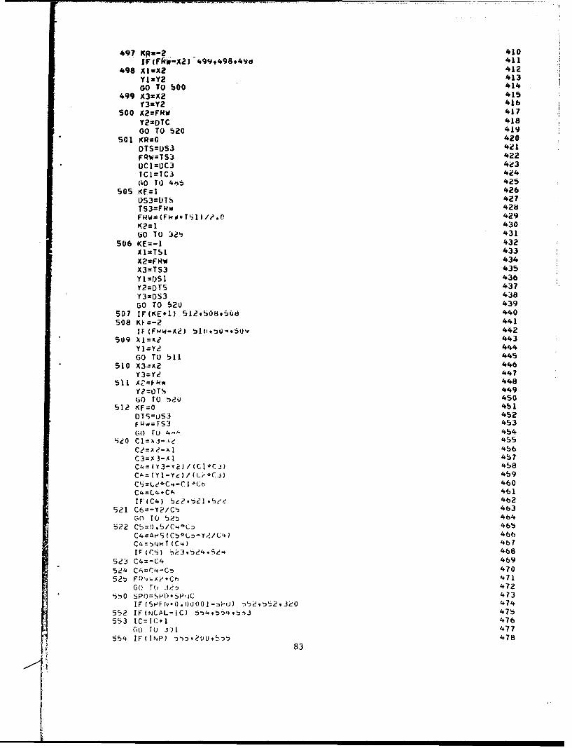
497 KR*-?.. 410JrcFRW-X2) 4.9994989496d 411

498 XlwXZ 412YlwY2 413Go to $600 414

499 A3xX2 415Y3zY2 416

500 X2=FRW 417

Y2O(TC 418GO TO 520 419

501 KR=O420DTS=US3 421FRW=TS3 422uc1ODC3 4ie3TCI=IC3 424G0 TO 46$ 425

505 KE=l 426US3=UTS 427TS3=Fkw 428Fww=(Fkm+Ts1 )/?.O 4e9K2=1 43000 ITo 32t 431

506 KE=-l 432xI=TSl 433A 2=FRW 434X3=TS3 435y I DS 1 436Y2=DTS 437Y3=DS3 438Go TO 520 439

507 IF(KE*1J 5129S08#50d 440508 KF=-2 441

* 5 I9 (Fww-X2) 5It',lt~'..St)' 442

Y1=Y,2 444

GO TO 511 445*510 X3jA2 446

Y3=Y2 447511 AZ"Fkw 448

Y?=IJTS 44960 TO ')20 450

512 KF=O 45LDTS=OS3 452F-w'=TS3 45360( TO 4-f 454

S20 Cl=XJ-.'d 455

C2=A?-A 1 456C3=A 3-Al 457C4= Y3-Yc3/((;1*C-5) 458

C" (Y-Ve) (L,*CJ)459C5L*C 14 -C I " t 460C4=C4*Ch 461

521 C6=-Y?/C3 463GO to bpt 464

522 Cb=0.5/C4*Ca 465C4=AHS (Ct)*C--Y?/Cr.) 466C4=13HT (C'4) 4b7IF-(C5) -,e,95d4o.-)&* 468

523 C4=-C4 469524 C6=('.-Cn 47052t) FR'výACtb. 4711

GO TO Jen 472

*i In 0 SPO=SPO+Spljc 473IF (SH-FNv+.0.U)OI-ýi-t) ~ 2JO474

5S2 IF(NCAL-IC) 5-4t5vj 475553 I=IC~l476

G o To u jI) 477554 IF(INP) '2O- 478

83

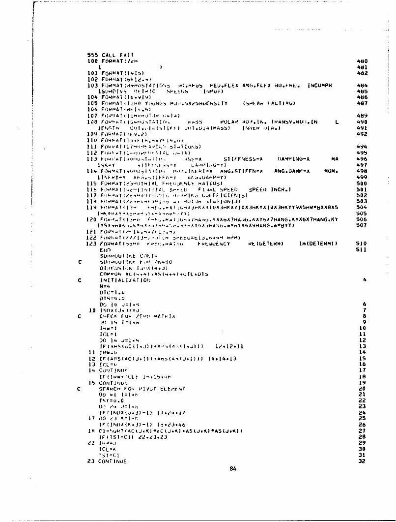
555 CALL FAIT1 48

101 F0kMAT(14.In)48102 FOP(4AT~bkle.n)103 FO~"!kTcm,#poSTAfT0N-) -40.ml-u) 1,EU*i'LEA AN(i.FLtA 114O.9Pkfu INCUMPH 484 j

104 F04MrAT(It,.v19) 406105 FOWIAT(1jHO Yý)UN(,j MPi;.:Ae'nML~fl%!rY (ýkmArq ýALT)@t,1 487

107 FOd'-lAT(11'sij-oTý),e 'i'.A) 489

1EF.r~Tr a'T~4'TI~ ill *uiA(MAhbi) IN'Jt. #)]A.) 491

110

113 1-S o~M Tu--li '½-A ST 1FFNiESSA ()AMPING- MA 496

114 FOWOAT141"U',31ýT1Qi r41 . I~tWT-A ANG*STIFFN-A ANGeDAI*'-A mom* 498

115 F0140MTl sýia'41IT"L Fti~-tjNiLl ttIIUTLO) S001l I FO4A .i:lfo .- L F.L Si~.Ei) SPEEt) INCH.) b01117 l'T(..ji'" LvtFi 1CIENTS) b02

120 Fow-i"r(lJimo F-ý-..fUI~U-IhA.'&AS,4AAOA7HA,,b(.iAYbA7MANG.KYXbX7t1ANG.KY 506~ 507

123 FORMAT (5-)-I ItuufNc'r R~~LWETLRM) IM(DETEIRM)) 510Emn 511

Siur4r)UI I jt\ cllý IC S(UpiouU I IN? f*.-)w P'N40O

C INITIAL114TlION 4N=4DrC=l .iu

06 10, J'=i*r 610 fNflA(J-, f)= 7

C C'.FCK FUl. ZEw( '4ATiIA a

onwi It 10-,4

1CL~l 11DO 14 J=1.N 12

11 Jpw=(, 1412 IF(APS(AC(JvI) )+Am-i(A'(Jqi) 3) 14914*13 1513 !CL=u 16

15 CONTPiNur 19C SFAR~CH FON ,PIV~r ELEmwNT 20

00 4.1 1=1.11 21TIST=u.0 22Ul' r". .3=1.N 23IFf INt`W(j.j)-I) 31It.,?.17 24

17 00 e3 K=1.f: 25

IM4 Cl=',uAk7(AC (J.K) *AC (J-lK) AS4JPA)*AS(J.K) 3 27IF(TSI-CL) 22923923 28

22 1Iko'j 29ICL-=% 30TST=Cl 31

23 CONTINUE 32

84

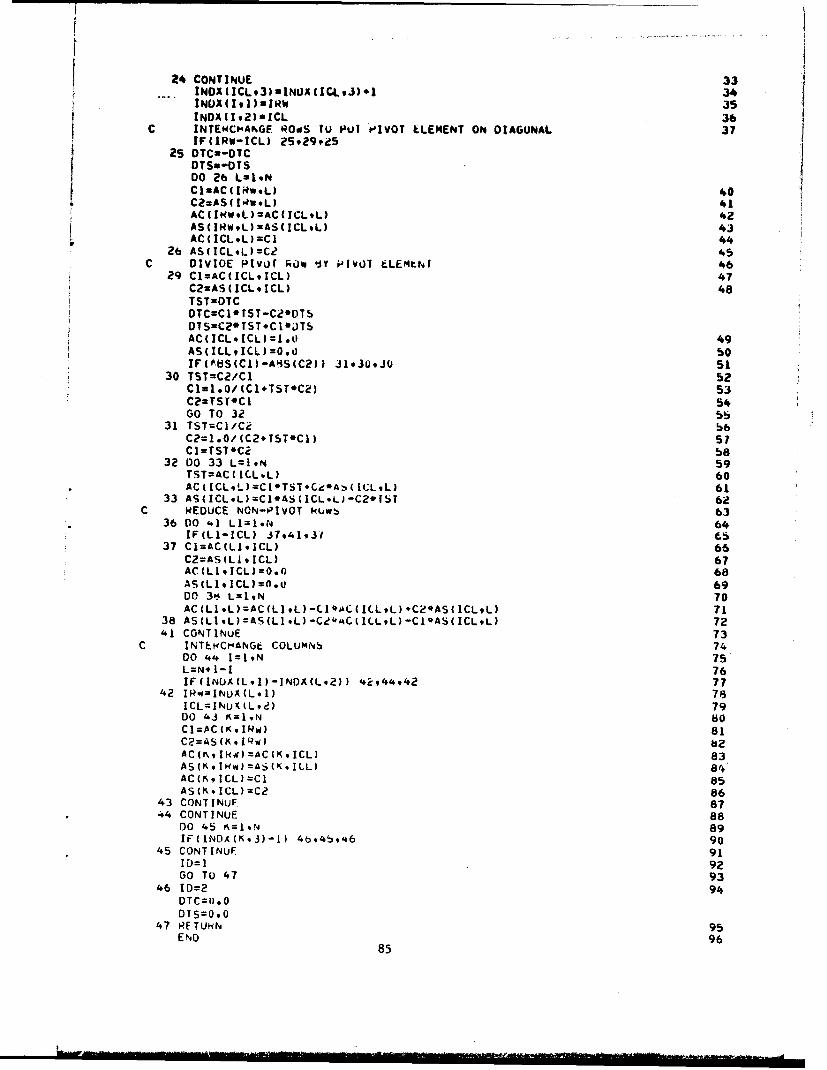
24 CONTINUE 33

INOX(I.13ImIRW 35INDA(192)*ICL 36

C INTEWCAENGE ROOS T ul PUI 1VOT LLEMENT ON DIAGONAL 37IF(IRW-ICL) 25929925

25 DTCz-DICDTSu-OTSDO 26 L*19NCImAC C 11wL) 40t C2=AS C 1**L) 41AC( I~WL)=AC( JCL*L) 42AS(RWWL)=AS( ICL*L) 43AC(ICLqL)=Cl 44

26 AS(ICLL3=C2 45C DvIVIE PIvUr 140% 4TY iIVqUl tLEMtNr 46

29 CI=AC(ICL9ICL) 47C2=AS(ICL*ICL) 48T STsOT COTC=C1*TST-C2*DTSD7SzC2*TST*Cl'*JTSAC(ICL*ICL)=1.0 49AS(ICLLICL)=O.0J b0JF(AIHS(C1)-A4iS(C2)) JI'JU.oJU 51

30 TST=C2/Cl 52C1= .0/ (C1.TST*C2) 53C2=TST*C1 54Go TO 32 55

31 TST=C1/C2 S6C2=1 .0/ CC2*T$T*C1 3 57C1=TS7*C2 be

32 DO 33 L=1.N 59TST=AC( IC.L*L) 60

*AC(ICLqLj=Ci*TST*Ce*AS)(LCLL) 6133 AS(ICL#L)=C1*AS(ICL*L1-C2*FST 6

C REDUCE NON-P~IVOT kUwb 63*36 00 41 L11I.N 64

IF(LI-ICL) 37941931 6*37 C1=AC(LIICL) 66

C2=AS(LI *ICL) 67AC (L * ICL3 =0.0 68AS(LI9ICL)=fl.u 69DO 3'" L1,vN 70

38 AS(L1.LI=AS(L1.L)-CeM'C(ILLL)-C1*AS(ICL.L) 7241 CONTINuE 73

C INTEtRCANGE COLUmNb 74DO 44' 1=19N7L=11441-1 76IF(INbA(l_*i)-JNOA(L.231 42944*42 77

42 IRW=INUX(Lol) 78ICL=INu4 (l_*2 79DO 43 K=1.N 80C1=AC(KeIRW) 81C2=AS (iK* I'RW b2AC(KIIk43=AC(K. ICL) 83A5(K*,1W)=AS(KoILL) 84.AC (KICL) =C1 85AS(K*ICL)=C2 86

43 CONTINUE a?*44 CONTINUE 88

DO 45 K=I*N 89IF (INDA (K, 33-I) 46@45,'.6 90

45 CONTINUE 91ID=1 92GO TO 47 93

46 1D=2 94

D7S=0.047 RETURN 95

END 9685

REFERENCES

1. Rotor-Bearing Dynamics Design Technology, Part V: "Computer Program Manualfor Rotor Response and Stability, Technical Report AFAPL-TR-65-45, Part V,J. W. Lund, May 1965.

2. Rotor-Bearing Dynamics Design lechnology, Part VII: "The Three Lobe Bearingand Floating Ring Bearing,"Technical Report AFAPL-TR-65-45, Part VII, J. W.Lund, February 1968.

3. Rotor-Bearing Dynamics Design Technology, Part VI: "The Influence of Electro-magnetic Forces on the Stability and Response of an Alternator Rotor,'Tech-nical Report AFAPL-TR-64-45, Part VI, J. W. Lund and T. Chiang, September1967.

4. Lund, J. W., "The Stabi~ity of an Elastic Rotor in Journal Bearings withFlexible, Damped Supports", Trans. ASME, Journal of Applied Mechanics, SeriesE Volume 87, pp. 911-920.

5. Lund, J. W., Wernick, R. J. and Malanoski, S. B., "Analysis of the HydrostatiJournal and Thrust Bearing for the NASA AB-5 Gyro Gimbal Bearing", MechanicalTechnology Inc., Report No. MTI-62TR26, 1962.

6. Hildebrand, F.B., "Introduction to Numerical Analysis", McGraw-Hill BookC., 1956, pp. 41-43.

7. Tang, I.C. and W.A. Gross, "Analysis and Design of Externally PressurizedGas Bearings", ASLE Paper No. 61LC-20, 1961.

8. Design of Gas Bearings, Vol. I, Mechanical Technology Inc., 1969, Section5.6.

86

UnclassifiedSecuirity Classification

DOCUMENT CONTROL DATA. R & D(Security classiflcation of title. body of abstract and indexind annotations mun, be entered when the overall report I classlfled)

I. ORIGINATING ACTIVIYT (Corpora•oteautho) ,. REPORT SECURITY CLASSIFICATION

Mechanical Technology Incorporated UnclassifiedGROUP

968 Albany-Shaker Road N/A

T.oj~p? Newj Vpvl 171103. REPORT •T1'kL"

Rotor-Bearing Dynamics Design TechnologyPart IX: Thrust Bearing Effects on Rotor-Bearing Stability

4. OtSCRIPTIVE NOTES (7'ype o report and inclusive dates)

Final Report for Feriod October 1968 to January 1969I. AU THORISI (First name, middle Initial, ltat name)

R.A. Candiff and .7. Vohr

C REPORT OATE 70. rOTAL NO. OF PAGES I-~ NO. OF REFS

August 10, 1970 97 8SM. CONTRACT OR GRANT NO, 90. ORIGINATOR'S REPORT NUMSERIS)

AF33(615)-3238 "b. PROJECT NO. 3048 i 70TR40

c. Task Nr: 304806 9b. OTHER REPORT NO'--) (Any other numbers that m.ay be assigedthis report)

d. Task Nr: 304806 AFAPL-TR-65-45, Part IX10, DISTRIBUTION STATEMENT

This document is subject to special export controls and each transmittal to foreigngovernments or foreign nationals may be made only with prior approval of the Air For eAero Propulsion Laboratory (APFL), Wright-Patterson Air Force Base, Ohio 45433.

I- SUPPLEMENTARY NOTES t2. SPONSORING MILITARY ACTIVITY

None Air Force Aero Propulsion LaboratoryWright-Patterson AFB, Ohio 45433

I1. ASSTRACT

This volume presents a study conducted to determine the effects thrust bearingson rotor-beariag stability. A computer program, written in order to study theseeffects, permits the inclusion of the thrust bearing characteristics into therotor system. A program manual is provided, containing a listing of the programand detailed instructions for preparation of input data. A technique is alsopresented which provides for the user a convenient method of evaluating thestability of a rotor system with and without the thrust bearing data. Extensivedesign data are presented for gas-lubricated, externally pressurized thrustbearings.

DDD 14°VS "1473 ( UnclassifiedS/N 0101.-807-6801 Security ClAssification

UnclassifiedSecurity Clansification

14 LINK A LINK S LINK CK[Y WOROS-

ROLE WT ROLE WT O ROLE WT

Bearings

Critical Speed

Lubrication

Fluid Film

Hybrid

Hydrodynamic

Hydrostatic

Rotor-Bearing Dynamics

Stability

Stiffness and Damping

Gas Lubrication

Gas Bearings

FORM.,BCDD 040V0.1473 UBCK) unclassified(PAGE- 2) Security Classification