New perspectives on climate, Earth surface processes and

New perspectives on climate, Earth surface processes and thermal–hydrological conditions in high–latitude systems

juha aalto

Department of Geosciences anD GeoGraphy a29 / HElsiNki 2015

ACADEMiC DissERTATiONTo be presented, with the permission of the Faculty of science of the University of Helsinki, for public examination in lecture room 6, University main building, on 23 January 2015, at 12 o’clock noon.

ISSN 1798-7911 ISBN 978-952-10-9469-9 (paperback)ISBN 978-952-10-9470-5 (PDF)http://ethesis.helsinki.fi

UnigrafiaHelsinki 2015

© Juha Aalto (synopsis)© Springer (Paper I)© Regents of the University of Colorado (Paper II)© John Wiley and Sons (Papers III and IV)Cover photo: Juha Aalto

Author´s address: Juha Aalto Department of Geosciences and Geography P.O.Box 64 00014 University of Helsinki Finland [email protected]

Supervised by: Professor Miska Luoto Department of Geosciences and Geography University of Helsinki, Finland

Co–supervised by: Dr. Ari Venäläinen Finnish Meteorological Institute, Finland

Reviewed by: Professor Jan Hjort Department of Geography University of Oulu, Finland

Professor Alfred Colpaert Department of Geographical and Historical Studies University of Eastern Finland, Finland

Discussed with: Assistant Professor Stephan Harrison College of Life and Environmental Sciences University of Exeter, United Kingdom

Aalto J., 2015. New perspectives on climate, Earth surface processes and thermal–hydrological conditions in high–latitude systems. Unigrafia.Helsinki.38pagesand8figures.

abstract

Climate, Earth surface processes and soil ther-mal–hydrological conditions drive landscape de-velopment, ecosystem functioning and human activities in high–latitude regions. Such areas are characterized by large annual variations in air temperatures, frost–related geomorphic activity and extreme spatial heterogeneity of the ground surface conditions due to complex topographical and edaphic settings. These systems are at the focal point of concurrent global change studies as the ongoing shifts in climate regimes has al-ready changed the dynamics of fragile and high-ly specialized environments across pan–Arctic.

This thesis aims to 1) analyze and model ex-treme air temperatures, soil thermal and hydro-logical conditions, and the main Earth surface processes,ESP,(cryoturbation,solifluction,ni-vation and palsa mires) controlling the function-ing of high–latitude systems in current and future climate conditions; 2) identify the key environ-mental factors driving the spatial variation of the phenomenastudied;and3)developmethodolo-gies for producing novel high–quality datasets, which can be used in other applications and dis-ciplines, such as climatology, ecology and geo-science. To accomplish these objectives, spatial analyses were conducted throughout a range of geographical scales by utilizing multiple statis-tical modelling approaches, such as regression and machine learning techniques. The robust-ness of these models was further increased by adopting an ensemble approach, where the out-puts of different statistical algorithms were com-bined to give single agreement outputs. This the-

sis was based on unique datasets from north-ern Fennoscandia: climate station records from Finland, Sweden and Norway; state–of–the–art climatemodelsimulations;fine–scalefieldmea-surements collected in arctic–alpine tundra; and remotely-sensed geospatial data. The study area covers the main environmental gradients thus providing suitable study settings for theoretical and applied research in arctic–alpine environ-ments.

Overall, the models successfully related the geographical variation in investigated high–lati-tude phenomena to main environmental gradi-ents. In paper I, accurate extreme air tempera-ture maps were produced, which were notably improvedafterincorporatingtheinfluenceoflo-cal factors such as topography and water bodies into the spatial models. In paper II, the results show extreme variation in soil temperature and moisture over very short distances, while reveal-ing the factors controlling the heterogeneity of surface thermal and hydrological conditions. Fi-nally, the modelling outputs in papers III and IV provided new insights into the determination of geomorphic activity patterns across arctic–alpine landscapes, while stressing the need for accurate climate data for predictive geomorpho-logical distribution mapping. Importantly, Earth surface processes were found to be extremely climatic sensitive, and drastic changes in geo-morphic systems towards the end of 21st cen-tury can be expected. The increase over current temperaturesby2˚Cwasprojectedtocauseanear–complete loss of active ESPs in the high–

3

DEpARTMENT OF GEOsCiENCEs AND GEOGRApHy A29

4

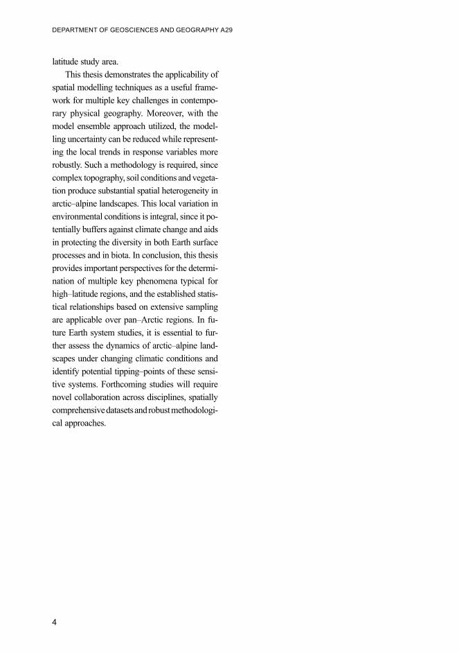
latitude study area.This thesis demonstrates the applicability of

spatial modelling techniques as a useful frame-work for multiple key challenges in contempo-rary physical geography. Moreover, with the model ensemble approach utilized, the model-ling uncertainty can be reduced while represent-ing the local trends in response variables more robustly. Such a methodology is required, since complex topography, soil conditions and vegeta-tion produce substantial spatial heterogeneity in arctic–alpine landscapes. This local variation in environmental conditions is integral, since it po-tentially buffers against climate change and aids in protecting the diversity in both Earth surface processes and in biota. In conclusion, this thesis provides important perspectives for the determi-nation of multiple key phenomena typical for high–latitude regions, and the established statis-tical relationships based on extensive sampling are applicable over pan–Arctic regions. In fu-ture Earth system studies, it is essential to fur-ther assess the dynamics of arctic–alpine land-scapes under changing climatic conditions and identify potential tipping–points of these sensi-tive systems. Forthcoming studies will require novel collaboration across disciplines, spatially comprehensive datasets and robust methodologi-cal approaches.

5

acknowledgements

I’ve been lucky to be surrounded by amazing people without whom this work would have been greatly diminished. First of all, I’m indebted to my supervisor, Prof. Miska Luoto for his crucial support and advice throughout this project. Dur-ing the past three years, he has always provided me time for constructive and critical discussions and not once I’ve needed to question his enthusi-astic vision. My co-supervisor Dr. Ari Venäläinen was also an important part of this project and I thank him for his support.

I would like to acknowledge the co-authors of the papers; I have had the privilege to work with exceptional talented scientists. Special thanks go to Dr. Peter C. le Roux; the multiple discussions with him at the slopes of Saana as well as at the officehavehadabiginfluenceonmywork.Ad-ditionally, I want to thank my reviewers, Prof. Jan Hjort and Prof. Alfred Colpaert for encour-aging and helpful comments.

I wish to thank Reija Ruuhela and Hilppa Gregow from FMI for support and providing me the opportunity to work on both sides of the street. I’m particularly thankful to my FMI-wolf-pack-leader Pentti Pirinen for helping me count-less of times with all sort of data related prob-lems. I also acknowledge Dr. Ewan O’Connor forpolishing the languageof thefinalversionof the manuscript.

Kilpisjärvi biological research station has been my second home for the past three years. Therefore I would like to thank the staff (espe-cially Pirjo!) for providing the facilities that a tiredfieldworkerneeds.Ialsothanktheresearch-ers and staff at the Department of Geoscienc-es and Geography for a friendly and supporting work atmosphere.

On a personal note, I thank my family: my two beautiful daughters Emma and Venla, my

mother Pirjo, and my twin sister Tuikku, for re-minding me what is important in life. Thanks for listening tirelessly to the latest updates on my work. Special thanks to Maija for love, help inthefieldandattheoffice,andallthesupport.

This work was funded by the Geography Graduate School of the Academy of Finland. Additionally, I would like to acknowledge the fundingbyOskarÖflundsStiflelse,SocietasProFauna et Flora Fennica, an University of Helsinki Grant, and Nordenskiold Sambundet.

Three other publications are also related to the PhD project, but have not been included in the thesis:1) Aalto, J., Pirinen, P., Heikkinen, J., Venäläinen, A. 2012. Spatial interpolation of monthly climate data for Finland: comparing the performance of kriging and generalized additive models. The-oretical and Applied Climatology 112, 99-111.2)leRoux,PC.,Aalto,J.,Luoto,M.2013.Soilmoisture’s underestimated role in climate change impact modelling in low-energy systems. Global Change Biology 19, 2965-2975.3)Aalto,J.,Luoto,M.2014.Field-measuredsoiltemperatureandmoisturedataimprovefine-scalemodels of periglacial activity patterns. Perma-frost and Periglacial Processes. Under review.


6

7

contentsAbstract ........................................................................................................................3Acknowledgements ......................................................................................................5List of original publications .........................................................................................8Authors’ contribution to the publications.....................................................................9Abbreviations .............................................................................................................10Listoffigures .............................................................................................................11

1 Introduction ........................................................................................................12

1.1 Background and motivation ...........................................................................12 1.2 Climate change context ..................................................................................13 1.3Methodologicaldevelopment .........................................................................14 1.4 Objectives of the thesis...................................................................................15

2 Material and methods ........................................................................................16

2.1 Study areas .....................................................................................................16 2.2 Climate data ....................................................................................................16

2.2.1 Climate station data ...............................................................................16 2.2.2 Derived climate indices .........................................................................18 2.2.3Globalclimatemodelsimulationdata ...................................................18

2.3Fielddata ........................................................................................................19 2.4 Geospatial data ...............................................................................................19 2.5 Statistical analysis ..........................................................................................21

3 Summary of original publications ....................................................................22

Paper I...................................................................................................................22 Paper II .................................................................................................................22 Paper III ................................................................................................................23 Paper IV ................................................................................................................23

4 Discussion ............................................................................................................24

4.1 The drivers of the investigated high–latitude phenomena ..............................24 4.2 Methodological issues ....................................................................................28 4.3Futureperspectives .........................................................................................30

5 Conclusions .........................................................................................................31

References ..................................................................................................................32Errata ..........................................................................................................................38

Publications I–IV

8

list of original publications

This thesis is based on the following publications:

I Aalto, J., le Roux, P.C., Luoto, M. 2014. The meso–scale drivers of temperature extremes in high–latitude Fennoscandia. Climate Dynamics42,237–252.

II Aalto, J.,leRoux,P.C.,Luoto,M.2013.Vegetationmediatessoiltemperatureandmoisture in arctic–alpine Environments. Arctic, Antarctic, and Alpine Research 45, 429–439.

III Aalto, J., Luoto, M. 2014. Integrating climate and local factors for geomorphologi-cal distribution models. Earth Surface Processes and Landforms 39,1729–1740.

IV Aalto, J., Venäläinen, A., Heikkinen, R.K., Luoto, M. 2014. Potential for extreme loss in high–latitude Earth surface processes due to climate change. Geophysical Research Letters41,3914–3924.

The publications are referred to in the text by their roman numerals.


9

authors’ contribution to the publications

І ThestudywasplannedbyM.Luoto.J.Aaltoconductedthedatacollection(datasynthesis, GIS analyses) and statistical analyses (multivariate regression). J. Aalto and P. C. le Roux were responsible for preparing the manuscript, while all authors commented and contributed.

ІІ ThestudywasplannedbyJ.AaltoandM.Luoto.Allauthorscontributedtofieldwork. J. Aalto and P. C. le Roux conducted statistical analyses (multivariate regres-sion). J. Aalto and P. C. le Roux were responsible for preparing the manuscript, while all authors commented and contributed.

ІІІ ThestudywasplannedbyM.LuotoandJ.Aalto.M.LuotoconductedtherelatedfieldinvestigationswhileJ.Aaltowasresponsiblefortheaerialphotographyin-terpretation, GIS analyses and statistical modelling. J. Aalto was responsible for preparing the manuscript, while M. Luoto commented and contributed.

ІV ThestudywasplannedbyJ.AaltoandM.Luoto.M.LuotoconductedtherelatedfieldinvestigationswhileJ.AaltowasresponsibleforthedatasynthesisandGISanalyses. J. Aalto conducted data analysis (down–scaling of the climate model data, statistical modelling). J. Aalto was responsible for preparing the manuscript, while A. Venäläinen, R. K. Heikkinen and M. Luoto commented and contributed.

10

abbreviations

ANN artificialneuralnetworkAUC area under the receiver operating characteristics curve CMIP3 coupledmodelintercomparisonprojectphase3CTA classificationtreeanalysisDEM digital elevation modelESP Earth surface processFDA flexiblediscriminantanalysisFDD freezing degree daysGa giga–annumGAM generalized additive modelGBM generalized boosting methodGCM general circulation modelGDM geomorphological distribution modelGIS geographical information systemGLM generalized linear modelMARS multiple adaptive regression splinesm a.s.l. meters above sea level MAXENT maximum entropyNW northwestPET potential evapotranspirationRF random forestSRE surface range envelopeSRES special report on emission scenariosSW southwestTDD thawing degree daysTMEAN mean annual temperatureTSS true skill statisticsTWI topographical wetness indexVWC volumetric water content (%)WAB water balance


11

List of figures

Fig. 1 Forecasted changes in mean temperatures and precipitation by the end of 21st century in northern Europe, page 14Fig. 2 The location of the study areas in high–latitude Fennoscandia, page 17Fig.3 The four key Earth surface processes (ESPs) occurring in the study area, page 20Fig. 4 An example of the modelled temperature and geomorphic activity, page 25Fig. 5 Schematic of the generalized patterns of high–latitude phenomena, page 26Fig. 6 The key drivers determining air temperature, ground thermal–hydrological con ditions, and ESP activity patterns, page 27Fig. 7 Ensemble forecasting of cryoturbation distribution under two different temperature conditions, page 29Fig. 8 The forecasted occurrence of nivation along increasing temperatures in relation to local topographic conditions, page31

12

1 introduction

1.1 Background and motivation

High–latitude environments are strongly con-strained by their latitudinal and altitudinal loca-tion which is generally characterized by a cold climate and pronounced topographical complex-ity (Bowman and Seastedt, 2001). In these sys-tems(located roughlyat60–90˚N/S),climaticconditions, soil thermal and hydrological re-gimes, and geomorphic activity drive the land-scape development, ecosystem functioning and human activities (Johnson and Billings, 1962; Washburn, 1979; Parmesan et al., 2000; Post et al., 2009). To cover these different aspects, this thesis is divided into three main themes: 1) climate, 2) soil thermal–hydrological conditions and3)Earthsurfaceprocesses. In theclimatepart of the thesis (paper I) the focus is on ex-treme annual air temperature variations, which potentially possess a major stress factor for biotic processes(Chapin,1983;Marchandet al., 2006; Zimmermann et al., 2009), and partly control the activity of Earth surface processes (ESP) in these systems (French, 2007). Additionally, lower at-mospheric conditions are strongly coupled with soil temperatures and moisture conditions which are further important drivers of vegetation assem-blages and frost–driven Earth surface processes in high–latitude environments (Swanson et al., 1988; Scherrer and Körner, 2010). Strong varia-tions in the annual temperature cycles (both air and insoil)are thereforedefiningelementsofarctic–alpine regions, shaping both the abiotic and biotic environment (Greenland and Losle-ben, 2001).

Soil thermal and hydrological conditions (the second part of the thesis, paper II) are the key determinants of ecosystem dynamics and geo-morphic activity in high–latitude regions (Lloyd

and Taylor, 1994; French, 2007; Bertoldi et al., 2010). These ground surface characteristics are the fundamental drivers of soil physical–chemi-cal processes, such as microbial activity, carbon cycling, nutrient availability and the activity of frost–related processes (Broll et al., 1999; Saito et al., 2009). Recent literature has recognized ex-treme temperature and moisture variations with-in distances less than one meter (Scherrer and Körner, 2010; le Roux et al.,2013a),thuscreat-ingamosaicofprocessesoperatingatfinespatialscales. Presumably, this spatial heterogeneity in ground thermal and hydrological patterns is ulti-mately driven by complex topographical settings, (Isard, 1986; Takahashi, 2005) and, within a few meters, may exceed long latitudinal or altitudinal gradients (Billings, 1974; le Roux et al.,2013a).

A manifestation of the broad scale geologi-cal and climatic factors and soil temperature and moisture, ESPs are characteristic features of arc-tic–alpine landscapes (papers III and IV) (Wash-burn, 1979; French, 2007). ESPs in these regions are mainly driven by the formation of ground ice in the topmost soil layer and the spatial distri-bution of permafrost (French, 2007; Etzelmül-ler,2013).Geomorphicsystemsare importantfactors effecting landscape and vegetation dy-namics in arctic–alpine systems (Malanson et al., 2012; Frost et al.,2013;leRouxet al.,2013b).In the third part of the thesis (papers III and IV), the focus is on four key ESPs occurring in high–latituderegions:solifluction,cryoturbation,nivation and palsa mires. Geomorphic features reflect the landscapeevolutionduring theHo-locene while processes still remain active today (Allard,1996).Solifluctionisgradualmasswast-ing driven by freeze–thaw cycles of the upper-most soil layers combined with gravity (Harris et al., 2001a; Matsuoka, 2005). These slow mass movements create various features such as lobes, steps and stripes (Matsuoka, 2001; Harris et al., 2008). Cryoturbation (frost churning) refers to


13

the mixing of materials from various horizons of the soil down to the bedrock due to freezing and thawing, generating features such as patterned ground and earth hummocks (Washburn, 1979; Matthews et al., 1998; French, 2007). Nivation represents local snow accumulation sites close-ly related to other hillslope processes including masswasting,weatheringandfluvialprocesses(Thorn, 1979; Wasburn, 1979; French, 2007). Palsa mires are mire complexes with a perma-nently frozen core (Seppälä, 1986), located at the outer margins of the discontinuous perma-frost zone in high–latitude peatlands (Luoto et al., 2004).

At regional scales (spatial resolution 10 km2–1000 km2), climatic conditions, such as average temperature and precipitation, has been found to control the geomorphic activity as well as soil thermal and hydrological patterns (Isard, 1986; Fronzek et al., 2006). These conditions, however, establish very general distributional patterns of response variables due to the spatial extent of the meteorological variables (Luoto et al., 2004; Pot-ter et al.,2013).Moreover,recentliteratureim-plies that towards the landscape and local scale (spatial resolution 1 km2 – 0.01 km2) other factors such as local topography, soil characteristics and vegetation, control the soil thermal–hydrologi-calpatterns,withgeomorphicactivityfilteringthe coarse–grained effects of climate and cre-ating distinct microclimatic spaces (Hjort and Luoto, 2009; Wundram et al., 2010; Scherrer and Körner, 2011; Graham et al., 2012; Malan-son et al., 2012). Further, the increasing level of spatial heterogeneity causes strong coupling and feedbacks among environmental gradients (both abiotic and biotic) (Isard, 1986; Ehrenfeld et al., 2005; le Roux et al.,2013a).Fromamethod-ological point of view, these connections can be challenging as the level of collinearity, i.e., the statistical association between explanatory vari-ables,tendstoincreasetowardsfinespatialscales

(Daly, 2006). This can further hinder the investi-gation of individual effects among variables and potentiallycausallinks(Graham,2003).

1.2 climate change context

Over the last decades, high–latitude regions es-pecially have experienced a rapid increase in mean temperatures (Serreze et al., 2000; IPCC, 2013).Simultaneously, thedynamicsof theselandscapes has changed; for example the veg-etation cover has increased notably in response to changing climatic conditions (Sturm et al., 2001; Tape et al., 2006) and fragile permafrost formations have started to degrade (Luoto and Seppälä,2003;Payetteet al., 2004; Bosiö et al., 2012). High–latitude regions may be very sen-sitive to climate warming due to their marginal location, specialized biota at their distributional limits and the fact that the projected relative rise in temperatures increases pole wards (Fountain et al.,2012;IPCC,2013)(Fig.1).Inaddition,various land surface conditions and permafrost in these environments are found to be strongly linked to the prevailing climate (Fronzek et al., 2006; Etzelmüller et al.,2013;Farbrotet al., 2013).Importantly,multipleenvironmentalgra-dients are potentially responding simultaneously to the changing climate, with an as yet uncertain rate and amplitude (Chapin et al., 2005; Starr et al., 2008; Virtanen et al., 2010).

Changes in arctic–alpine systems can trig-ger multiple opposing feedbacks with poten-tially global implications (Knight and Harrison, 2013).Forexample,warmerandwetterclimateconditions in the future can cause permafrost thaw to accelerate further, amplifying the deg-radation of palsa mire complexes (Payette et al., 2004; Fronzek et al., 2006). Similarly, dimin-ishing frost–activity enables vegetation to re–establish, which in turn stabilizes the topmost soilandfurthermodifiesheatfluxesandnutri-

14

ent cycles (Kade and Walker, 2008). The under-standing of such feedbacks is essential for cur-rent global change impact studies. For example, changes in land surface processes across pan–Arctic might effect ecosystem dynamics (Vir-tanen, et al., 2010; Macias–Fauria and Johnson, 2013)andloweratmosphericconditionsthroughvarious feedbacks related to changes in ground reflectance,heatfluxesandbiochemicalcycles(Callaghan et al., 2011; Koven et al., 2011; Pear-son et al.,2013).Moreover,permanentlyfrozenpeat soils are major storages of organic carbon, and the thawing of these releases greenhouse gases (CO2, CH4 and N2O) with potentially ma-jor effects on the climate system (Christensen et al., 2004; Bosiö et al., 2012). In this thesis, the impacts of climate change were examined in a predictive geomorphological context (paper IV).

1.3 methodological development

The spatial modelling of response variables and theidentificationofthemostinfluentialpredic-tors is an essential theme in contemporary en-vironmental and climate change impact studies (Guisan and Thuiller, 2005; Hjort and Luoto, 2009; Boeckli et al., 2012). Modern statistical approaches (e.g., Breiman, 2001; Venables and Ripley, 2002; Luoto and Hjort, 2005; Elith et al.,2008)provideflexiblemethodsforcapturingmultivariate relationships between response and environmental predictors across large geographi-cal gradients (Walsh et al., 1998; Hjort and Luo-to,2013),connectionsthatareoftenaccompa-nied by nonlinearities and thresholds (Schumm, 1979;Phillips,2003;HjortandLuoto,2011).Moreover, different predictor variables often possess a distinct effective scale (Daly, 2006; Potter et al.,2013), indicating that thespatialextent of the predictors’ effect might vary, e.g.,

figure 1. Forecasted changes in A) mean temperatures (∆ T) and B) precipitation (∆ RR) by the end of 21st century in northern Europe based on the ensemble of 19 general circulation models (GCM) (special report on emission scenarios [SRES] scenario A1B assuming CO2 emission roughly equal to 700 parts per million, baseline period 1971–2000). The black boxes indicate the approximate location of the study domain.


15

from regional to local (i.e., 1000 km2–0.01 km2). Therefore, a useful approach for examining the influenceofvariousenvironmentalfactorsonre-sponse variables is through a hierarchical model-ling perspective (Walsh et al., 1998; Albrecht and Car,1999;PearsonandDawson,2003).Moreprecisely, this encompasses the integration of different data sources e.g., climate, topography and soil into spatial models in stepwise man-ner (e.g., Pearson et al., 2004; Sormunen et al., 2011). Consequently, such a modelling approach helps to conceptualize and structure the effects of environmental drivers on response variables (papers I and III).

However, uncertainty in spatial modelling is introduced to the study from a variety of sources, for example sampling errors, inaccuracies in geo-spatial datasets and modelling algorithms (Walsh et al., 1998; Guisan and Zimmermann, 2000). The choice of the most suitable modelling tech-nique can be challenging since different statis-tical algorithms have their own strengths and weaknesses (Luoto and Hjort, 2005; Marmion et al., 2008). Recently, the compilation of en-semble prediction, i.e., the spatial forecast based on the outputs of multiple different modelling methods, has gained momentum in the environ-mental sciences (Marmion et al., 2009; Gallien et al., 2012). By utilizing such an approach, it is possible to examine the majority trends in data while considering the methodology related un-certainty (Araújo and New, 2007; Marmion et al., 2009). Moreover, this is especially useful when extrapolating the modelled present day patterns to future (or past) environmental conditions, as the predicted patterns of a single technique inside an ensemble might differ notably depending on the algorithm (Thuiller, 2004; Araújo et al., 2005; Fronzek et al., 2011). In this thesis, the ensemble modelling approach was utilized for predicting geomorphic activity patterns in current and future climate conditions (papers III and IV).

1.4 objectives of the thesis

This thesis has three main objectives: firstly to an-alyze and model the spatial variation in extreme temperatures (paper I), ground thermal–hydro-logical conditions (paper II), and geomorphic activity patterns (paper III), which are impor-tant controllers of high–latitude environments. Moreover, paper IV examines the climatic sen-sitivity of the four key ESPs, after modifying the prevailing temperature and precipitation re-gimes. Secondly, the aim is to identify the most influential factorsdriving thespatialvariationin described response variables under realistic multivariate settings. Thirdly, this thesis aims to provide new perspectives on the links and feedbacks among various environmental gradi-ents operating in the arctic–alpine regions, while developing methodologies for producing spatial datasets to be used by other applications and dis-ciplines, such as ecology and geoscience. To ac-complish the described objectives, spatial anal-yses were conducted across large geographical gradients utilizing modern statistical modelling approaches,comprehensivefield–quantifiedob-servations and remotely sensed geospatial da-ta sources. By assessing the climatic sensitivity of various land surface processes, this thesis at-tempts to deepen public discussion about impacts of climate change in high–latitude regions, and furtherstrengthenthescientificunderstandingofthese environments.

16

2 material and methods

2.1 study areas

In this thesis, temperature extremes, soil ther-mal–hydrological conditions and ESPs were modelled, focusing on multiple study areas in high–latitude Fennoscandia (Fig. 2). This region covers extensive environmental gradients with low human disturbance, thus providing an ideal location for spatial modelling studies and global change investigations. In general, the cold cli-mate of this region is affected by its northern lo-cation, the strong continental–oceanic gradient and the Scandes mountains (Tikkanen, 2005). The study area represents the marginal zone of discontinuous permafrost (Fig. 2a) (Christiansen et al., 2010). Based on the climate station data used in paper I (n=61; Fig. 2b), the mean annual temperature over the period of 1971–2000 was –0.3°C.However,duetoastrongland–oceangradient and pronounced topographical varia-tions, the mean annual temperature drops from 4.3°C(Borkenes,Norway;N68°46’S16°15’,36metersabovesealevel[ma.s.l.])to–3.6°C(KilpisjärviSaana,Finland;N69°2’S20°49’,1007 m a.s.l.) over a distance of approximate-ly 190 kilometers. Similarly, the mean annual precipitationsumis549mm,rangingfrom323mm(AbiskoScientificResearchStation,Swe-den;N68°21’S18°49’,394ma.s.l.)to1049mm(Tromsø,Norway;N69°39’S18°56’,100m a.s.l).

Due to the long–term development of the bed-rock(0.4–3.0Ga),topographyvariesthroughoutthe study domain with the highest fell tops lo-cated in the geologically younger regions of the study area of Caledonian rocks (i.e., Scandes at the west). The middle and southern parts con-sist of eroded Precambrian bedrock with a gently sloping landscape (Laitakari, 1998). This part of

Fennoscandia is mainly covered by glacigenic till deposits, peat soils and bare rock, but sandy es-ker formations from Weichselian glaciations are also widespread. Vegetation shifts from spruce (Picea abies) and Scots pine (Pinus sylvestris) dominated forests in the south, to mountain birch (Betula pubescens ssp. czerepanovii) in the north of the study area. Alpine vegetation, above the tree line, is characterized by shrubs (e.g., Betu-la nana, Juniperus communis ssp. alpina) and dwarf–shrubs (e.g., Empetrum hermaphroditum) (Sormunen et al., 2011; le Roux et al., 2014).

In this thesis, each case study (papers I–IV) represents a subset of the described geographi-cal domain (Fig. 2). The study area in paper I is locatedbetween68˚Nand70˚N(Fig.2binpaper I). The two study sites in paper II are lo-cated approximately 100–200 m above the tree line on the Saana massif, both at an elevation of ca. 700 m a.s.l. (Fig. 2d). The study areas in papers III and IV cover ca. 20 000 km2 and 26 000 km2, respectively, mainly in north–western Finland (including minor parts from Sweden and Norway) (Fig. 2c).

2.2 climate data

2.2.1 Climate station data

The temperature dataset used in paper I cov-ers the period 1971–2000 and comprises 61 sta-tions covering the northern parts of Fennoscan-dia from the national observation networks of Finland, Sweden and Norway. The observations were collected from the climate databases of the Finnish Meteorological Institute and other na-tionalmeteorologicalofficesandresearchsta-tions(AbiskoScientificResearchStation2012;Norwegian Meteorological Institute, 2012; Swedish Meteorological and Hydrological In-stitute, 2012). Daily minimum, maximum and mean temperatures were extracted from station


17

figu

re 2

. Th

e lo

catio

n of

the

stu

dy

area

s in

hig

h–la

titud

e Fe

nnos

cand

ia.

pane

l A

show

s th

e st

udy

area

in

rela

tion

to t

he c

ircum

pola

r ex

tent

of

perm

afro

st (b

ased

on

the

data

in B

row

n et

al.,

199

8),

indi

cate

d as

fol

low

ing:

co

ntin

uous

=90–

100

% o

f th

e ar

ea

cove

red

by p

erm

afro

st, d

iscon

tinuo

us=

50–9

0 %

, spo

radi

c=10

–50

%, i

sola

ted=

<1

0 %

, res

pect

ively.

Pan

el B

pre

sent

s th

e cl

imat

olog

ical

st

atio

n ne

twor

k ut

ilized

in p

aper

i (n

=61)

. The

act

ivity

of

geom

orph

ic pr

oces

ses f

or p

aper

s iii a

nd

iV w

as m

appe

d at

loca

tions

sho

wn

at

pane

l C (n

=120

0). T

he tw

o st

udy

sites

(N

W =

nor

thw

est;

sW =

sou

thw

est)

of

the

fine–

scal

e da

tase

t us

ed in

pap

er

ii is

sho

wn

in p

anel

D w

ith 1

00–m

–in

terv

al co

ntou

r line

s ind

icatin

g ele

vatio

n.

in C

, th

e m

ap r

epre

sent

s th

e m

ean

annu

al a

bsol

ute

min

imum

tem

pera

ture

ov

er

the

perio

d of

19

71–2

000.

18

records and were used to determine annual ab-solute extremes and mean annual temperatures. The average of the yearly values across the pe-riod 1971–2000 was subsequently used in paper I to analyze the spatial variations of the temper-ature parameters.

2.2.2 Derived climate indices

In papers III and IV, the distributional patterns of ESPs were investigated in relation to four climate indices: mean annual temperature (TMEAN), freezing degree days (FDD), thawing degree days (TDD) and water balance (WAB). Such predictors have been shown to correlate with the occurrence of permafrost features in high–lati-tude regions (Luoto et al., 2004; Fronzek et al., 2006). To obtain the climatic indices, monthly mean temperatures and annual precipitation sum weremodelledbasedon thestatisticalspecifi-cations (generalized additive model; GAM) in paper I, accounting for topography, water cover and geographical location. The FDD and TDD are based on effective temperature sum below andabovebasetemperature(0˚C),respectively(Carter et al., 1991):

FDD = ∑ (𝑇𝑇𝑖𝑖 − 𝑇𝑇𝑏𝑏)𝑛𝑛𝑖𝑖=1 , if (Ti – Tb) < 0, (1)

TDD = ∑ (𝑇𝑇𝑖𝑖 − 𝑇𝑇𝑏𝑏)𝑛𝑛𝑖𝑖=1 , if (Ti – Tb) > 0, (2)

where, Ti denotes the mean temperature at day i, Tb the base temperature, and n the length of the summation period. However, as daily tempera-ture data was not available for this thesis, we es-timated FDD and TDD using monthly data (fol-lowing e.g., Araújo and Luoto, 2007). WAB was calculated as the difference between the mean annual precipitation sum and potential evapora-tion (PET) following Skov and Svenning (2004):

where T denotes the monthly mean temperatures. To predict the activity patterns of ESPs under current and future climates, these four indices were subsequently averaged to a spatial resolu-tion of 200 m × 200 m (ArcGis 10.1 Zonal Sta-tistics –function).

2.2.3 Global climate model simulation data

Climate projections for the 21st century are based on an ensemble of 19 global climate model sim-ulations obtained from the coupled model in-tercomparisonprojectphase3(CMIP3)archive(Meehl et al., 2007). In this thesis, the future cli-mate over two periods, from 2040 to 2069 and from 2070 to 2099, was calculated by adding the mean change as predicted by the 19 gen-eral circulation models (GCM) to the observed 1971–2000 climate (spatial resolution 10 km × 10 km) (Jylhä et al., 2009). The data represents the average changes in temperatures and precipi-tation under the B1, A1B and A2 emission sce-narios(Nakićenovićet al., 2000); B1 represent-ing low, A1B medium and A2 high greenhouse gas emissions, leading to CO2 concentrations at the end of the 21st century of roughly 540, 700 and above 800 parts per million, respectively. In order to match the resolution of the modelled baseline climate, the GCM data was bi–linear-ly downscaled to 200 m × 200 m. For the sen-sitivity analysis in paper IV, constant changes were applied to modelled monthly climate data; changesintemperaturefrom–2°Cto+6°Cat0.5°Cintervals,andofprecipitationfrom–50%to 50 % at 10 % intervals were tested. In paper IV, the climate predictors used (i.e., TMEAN, TDD, FDD and WAB) were re–calculated for each sensitivity and emission scenario analysis.


PET = 58.93 × Tabove 0 ̊ C / 12, (3)

19

2.3 field data

The spatial variation in soil temperature and moisture (paper II)wereinvestigatedinafine–scale study setting; on the Saana massif six sam-pling grids were established at two sites, with each grid comprising 160 1 m2 plots in a regular 8 x 20 arrangement. Both response variables were measured on two consecutive days (northwest-ern site; 16 July 2012; southwestern site: 17 July 2012) from a depth of 10 cm using a handheld digital temperature probe VWR–TD11 (VWR international, Radnor, Penn., USA; accuracy of 0.8°C).Volumetricsoilmoisturewasmeasuredusingahand–held time–domainreflectometrysensor (FieldScoutTDR300;SpectrumTech-nologies,Plainfield,IL,USA)uptoadepthof10cm,takingthemeanofca.3measurementsper quadrat.

In addition to the two response variables, three groups of predictors (each comprising of four variables) were measured and/or calculat-ed: topography, soil characteristics and vegeta-tion (le Roux et al.,2013a;Modet al., 2014). The four predictor variables related to topogra-phy were: mesotopography (a measure of local topography: 1=depressions, 10=ridge tops; see Billings,1973;Bruunet al., 2006), slope angle, potential annual direct radiation, and elevation. The four soil predictors were: soil temperature (when modelling soil moisture), soil moisture (when modelling soil temperature), peat depth, and the cover of rock. Finally, the four predictors in the vegetation group were: vegetation volume, biomass, cover of moss, and cover of lichen. The detailed description of the measuring protocol and predictors is provided in paper II.

In the geomorphology part of this thesis (pa-pers III and IV), the focus was on the activity patterns of four ESPs occurring in arctic–alpine regions:solifluction(Fig.3a),cryoturbation(Fig.3b),nivation(Fig.3c),andpalsamires(Fig.3d).

High–resolution aerial photography (spatial reso-lution of 0.25m2;LandSurveyofFinland,2013)andtargetedfield investigationswereusedforthe compilation of the geomorphological dataset (see e.g., Luoto and Hjort, 2005). The activity of the ESPs (1=presence, 0=absence) was visu-ally estimated based on the evidence in topsoil material e.g., mass wasting, frost–heaving and cracking as well as soil displacement (le Roux and Luoto, 2014). In paper III, the geomorpho-logicaldatasetcomprised1150observations(531sites visited). Moreover, this dataset was com-plemented in paper IV by increasing the total number of observations to 1200.

2.4 Geospatial data

A wide range of geospatial information sourc-es and geographical information system (GIS) techniques (ArcGis 10.1 Spatial analyst –func-tions) was utilized throughout this thesis. In pa-per I, the extreme temperature variations were modelled in relation to topography, water cover and geographical location. The digital elevation model (DEM) used is a global Gtopo with a spa-tialresolutionof30arcseconds(900m;USGS,2004). The land cover data was obtained from the Corine land cover 2006 dataset with a spatial resolution of 100 m × 100 m (European Environ-ment Agency, 2012). The water cover variables werespatiallyfilteredwithvaryingkernelsizesto account the gradually diminishing effects of the Arctic Ocean and lake cover (ArcGis 10.1 Focal statistics –function).

In addition to the climatic predictors de-scribed in section 2.2, papers III and IV focus on relating the activity patterns of ESPs with topographical, soil and vegetation variables (pa-per III). Two DEMs were utilized with differ-ent spatial resolutions: 1) 25 m × 25 m (Land SurveyofFinland,2013;paperIII)and2)30m×30m(NASALandProcessesDistributedActiveArchiveCenterLPDAAC,2013;paper

20

IV). From these DEMs, four terrain parameters were derived: slope angle, topographical wetness index (TWI) (Beven and Kirkby, 1979), poten-tial annual direct solar radiation (MJ/cm2/a), and total curvature (positive value indicating ridge tops and negative values valley bottoms). TWI was calculated using a Python script written by PrasadPathak(Esri,2013),whereaspotentialan-nual direct solar radiation (McCune and Keon, 2002)wascalculatedusingArcView3.2Solar analyst –extension accounting for latitude, slope angle and slope aspect.

The three soil predictors used in papers III and IV were peat cover, bare rock and sand cover. Thesoilclasseswerereclassifiedfromthedigi-tal soil database (Geological Survey of Finland, 2010; spatial resolution of 20 m × 20 m) and thebinarymaskscreatedwerespatiallyfilteredto a continuous scale. Additionally, two vegeta-tion variables were included in the analysis of

paper III: coniferous forest cover (%) and de-ciduous forest cover (%). The vegetation data was compiled from the Corine 2006 land cov-er –dataset with a spatial resolution of 25 m × 25 m (Finnish Environmental Institute, 2006). To obtain spatial predictions of the ESPs across the two study areas, all the predictors described in this section were resampled to 200 m × 200 m resolution by spatial averaging (ArcGis 10.1 Zonal statistics –function).

figure 3. The four key Earth surface processes (ESPs) occurring in the study area: A) solifluction (20°59’E 68°59’N, ca. 810 m a.s.l); B) cryoturbation (21°4’E 68°59’N, ca 880 m a.s.l); C) nivation (local snow accumulation site, 20°48’E 69°3’N, ca. 800 m a.s.l); and D) palsa mire (21°25’E 68°43’N, ca. 408 m a.s.l). Photos: A–C, Author, and D, M Luoto.


21

2.5 statistical analysis

The response variables in relation to multiple explanatory variables were examined within a spatial modelling framework (see e.g., Guisan and Zimmermann, 2000; Marmion et al., 2008; Ridefelt et al., 2010), in which the geograph-ical distribution of a response variable is sta-tistically associated with present environmental conditions. In this thesis, ten different statisti-cal modelling techniques were used (Thuiller et al.,2013), ranging fromparametric regres-siontocomplexmachinelearningandclassifi-cation methods (e.g., Breiman, 2001; Venables and Ripley, 2002; Luoto and Hjort, 2005; Elith et al., 2008). Such techniques included: general-ized linear model (GLM), generalized additive model(GAM),artificialneuralnetwork(ANN),classification treeanalysis (CTA),generalizedboosting method (GBM), random forest (RF), multiple adaptive regression splines (MARS), surfacerangeenvelope(SRE),flexiblediscrim-inant analysis (FDA) and maximum entropy (MAXENT). These modelling methods are de-scribed in more detail in papers I–IV. The en-semble modelling approach adopted in papers III and IV combines the outputs of different al-gorithms (with varying performance) to a single agreement prediction. This technique allows for accounting for the uncertainty related to differ-ent modeling techniques and their underlying as-sumptions (Walsh et al., 1998; Guisan and Zim-merman, 2000), further improving the predic-tive performance of geomorphical distribution models (GDM) (Marmion et al., 2009; Gallien et al., 2012).

Throughout this thesis, a cross–validation approach was used to evaluate the spatial mod-els. However, instead of splitting the data once for model calibration and evaluation (a common split–sample approach; Van Houwelingen and Le Cessie, 1990), this procedure was repeated

multiple times (e.g., 1000 runs in paper II) to account for sampling variability. This produces a distribution of the evaluation metrics of inter-est, rather than a single value. For continuous response variables (paper I and II), the model evaluation was based on the amount of deviance explained by the models (i.e., the goodness of the fit)andthepredictiveperformancei.e.,howwellthe predicted values explained the observed ones. In papers III and IV, the predicted occurrences of ESPs were evaluated using the area under the receiver operating characteristics curve (AUC) and true skill statistics (TSS). AUC is a thresh-old–independent measure of predictive accuracy assessing the agreement between the observed presence/absence values and model predictions (Fielding and Bell, 1997). The AUC values range from zero to one; a model providing excellent predictive performance has an AUC value higher than 0.9 and a fair model has AUC values ranging from 0.7 to 0.9 (see Swets, 1988). TSS is an ac-curacy measure that takes into account sensitiv-ity(truepositiverate)andspecificity(truenega-tive rate) and is not sensitive to prevalence (i.e., the frequency of occurrence). TSS ranges from –1 to 1, where 1 indicates perfect agreement, 0 random performance and –1, perfect disagree-ment (Allouche et al., 2006).

Additionally, two statistical techniques were used to calculate the relative importance of envi-ronmental factors in multivariate study arrange-ments: 1) variation partitioning, based on GLMs, parcels out the independent or joint contribution of variable groups (Borcard et al., 1992); while 2) variable importance in BIOMOD2identifiesthe relative importance of individual predictors (Thuiller et al,.2013).Moreprecisely,thevari-able importance compares correlations between thefittedvaluesandpredictions(thusindepen-dent from the techniques used) where the pre-dictor of interest has been randomly permutated. High correlation (i.e., the two predictions show

22


little difference) indicates that the predictor per-mutated is not considered important for the mod-el. Subsequently, each of the predictors is ranked basedonthecorrelationcoefficientsandthepro-portionoftherelativeinfluenceisscaledfrom0 to 1. Hence, the higher the variable impor-tance,themoreinfluentialthepredictorisinthemodel. The two methods described are useful to overcome statistical pitfalls such as collinearity amongthepredictors(Graham,2003).Allsta-tistical analysis in this thesis was conducted in the R statistical programming environment (R Development Core Team, 2011).

3 summary of original publications

paper i

Paper I focuses on investigating the meso–scale air temperature variations in topographically complex high–latitude environments. More pre-cisely, mean annual absolute temperature max-ima and minima, and mean annual temperature in Northern Fennoscandia were modelled by combining digital elevation model and remote-ly sensed land cover data with 61 climate series from northern Finland, Norway and Sweden. GAM and GLM were used to relate the varia-tion in air temperature extremes to the predictors andtopartitiontheresponsetothemostinflu-ential environmental variables.

The results indicate that minimum tempera-tures at the meso–scale are mainly driven by wa-ter cover variables. The effects were positive with proximity to Arctic Ocean generally increasing minima, while the lowest temperatures are most likely to occur at topographical depressions such as large mires and frozen lakes. In turn, maxi-mum temperatures were most strongly controlled by topography. Elevation, particularly, showed

the strongest effects due to the vertical lapse rate. Additionally, temperature maxima were re-lated to the sea proximity, which tends to buf-fer temperature variations and further decreas-ing maximum temperatures. Thus, the highest temperature maxima in the study area are likely to occur at low elevation sites at considerable distance from large water bodies. The models mainly associated the spatial variation of mean temperatures with geographical location and to the proximity of the Arctic Ocean. These results thus underline the governing role of oceanic and topographical gradients as the key meso–scale drivers of temperature variations in this high–lati-tude region. Moreover, the valuable outputs of this paper were the accurate temperature maps describing the meso–scale variation in extreme and mean temperature conditions. Subsequently, these forecasts were used in the later part of this thesis as GDM input data (papers III and IV).

paper ii

In paper II,thefine–scalevariationinsoiltem-peratureandmoisturewasquantifiedatanarc-tic-alpine site in northern Europe. Additionally, by utilizing GAM and GLM modelling and a robust cross–validation scheme, the effects of vegetation in controlling thermal and hydrologi-cal patterns were examined.

Soiltemperaturewasfoundtovaryby≥5˚Candmoistureby≥50%volumetricwatercontent(VWC)oververyshortdistances(≥1m).Theseresultsthusreflecttheextremespa-tial heterogeneity of thermal and hydrological conditions in these arctic–alpine systems. The inclusionofvegetationvariables significantlyimprovedboththemodelfitandthepredictiveperformance of the spatial models. While veg-etation showed marked effects on the studied parameters, the abiotic variables such as local topography and soil characteristics were the most

23

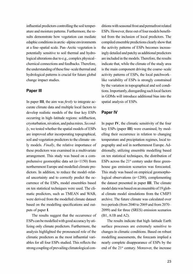
influentialpredictorscontrollingthesoiltemper-ature and moisture patterns. Furthermore, the re-sults demonstrate how vegetation can mediate edaphic conditions in arctic–alpine environments atafine–spatialscale.Pan–Arcticvegetationispotentially sensitive to soil thermal and hydro-logical alterations due to e.g., complex physical–chemical connections and feedbacks. Therefore, theunderstandingofthesefine–scalethermalandhydrological patterns is crucial for future global change impact studies.

paper iii

In paper III, the aim was firstly to integrate ac-curate climate data and multiple local factors to develop realistic models of the four key ESPs occurringinhigh–latituderegions:solifluction,cryoturbation, nivation, and palsa mires. Second-ly, we tested whether the spatial models of ESPs are improved after incorporating topographical, soil and vegetation predictors to the climate–on-ly models. Finally, the relative importance of these predictors was examined in a multivariate arrangement. This study was based on a com-prehensive geomorphic data set (n=1150) from northernmost Europe and modelled climate pre-dictors. In addition, to reduce the model–relat-ed uncertainty and to correctly predict the oc-currence of the ESPs, model ensembles based on ten statistical techniques were used. The cli-matic predictors, such as TMEAN and WAB, were derived from the modelled climate dataset basedonthemodellingspecificationsandout-puts of paper I.

The results suggest that the occurrence of ESPs can be modelled with good accuracy by uti-lizing only climate predictors. Furthermore, the analysis highlighted the pronounced role of the climaticpredictorsasthemostinfluentialvari-ablesforallfourESPsstudied.Thisreflectsthestrong coupling of prevailing climatological con-

ditions with seasonal frost and permafrost related ESPs.However,threeoutoffourmodelsbenefit-ted from the inclusion of local predictors. The compiled ensemble predictions clearly show that the activity patterns of ESPs becomes increas-ingly detailed and patchy as additional predictors are included in the models. Therefore, the results indicate that, while the climate of the study area is the main component driving the coarse–scale activity patterns of ESPs, the local patchwork–like variability of ESPs is strongly constrained by the variation in topographical and soil condi-tions. Importantly, disregarding such local factors in GDMs will introduce additional bias into the spatial analysis of ESPs.

paper iV

In paper IV, the climatic sensitivity of the four key ESPs (paper III) were examined, by mod-elling their occurrence in relation to changing temperature and precipitation regimes, local to-pography and soil in northernmost Europe. Ad-ditionally, utilizing ensemble modelling based on ten statistical techniques, the distribution of ESPs across the 21st century under three green-house gas emission scenarios was forecasted. This study was based on empirical geomorpho-logical observations (n=1200), complementing the dataset presented in paper III. The climate model data was based on an ensemble of 19 glob-alclimatemodelsimulationsfromtheCMIP3archive. The future climate was calculated over two periods (from 2040 to 2069 and from 2070–2099) and for three (SRES) emission scenarios (B1, A1B and A2).

The results indicate that high–latitude Earth surface processes are extremely sensitive to changes in climatic conditions. Based on robust modelling assessments, the forecasts implied a nearly complete disappearance of ESPs by the end of the 21st century. Moreover, the increase

24


inbaselineclimateconditionsby2̊ Cwasfoundto result in a drastic decrease in geomorphic ac-tivity in the study area. Similarly, studied ESPs strongly responded to manipulated precipitation conditions. The sites where geomorphic activ-ity was maintained were characterized by high altitude, compound topography and low radia-tion input generally associated with north–facing slopes. These results thus stress the sensitivity of ESP activity to altering climatic conditions in arc-tic–alpine systems. Moreover, this study shows the potential buffering effects of topographical and soil conditions against climate change, fur-ther promoting the local persistence of ESPs. The forecasted changes in geomorphic systems could have major impacts on both vegetation and regional climate system through changes in albedo,heatfluxesandbiogeochemicalcycles.This is thefirst study toexamine theclimaticsensitivity of multiple ESPs at landscape–scale while also accounting for local factors.

4 Discussion

4.1 the drivers of the investigated high–latitude phenomena

By modelling multiple key high–latitude phe-nomena, this thesis has provided new perspec-tives on climate, Earth surface processes and thermal–hydrological conditions across arctic–alpine landscapes. The results, based on exten-sive datasets and modern multivariate statistics, suggest diverse process–environment relation-ships which are organized in a hierarchical man-ner. Additionally, the analysis has provided new alarming evidence for the climatic sensitivity of high–latitude Earth surface processes. The spa-tial modelling framework and the ensemble–ap-proach utilized throughout the thesis have prov-entobeimportantanalyticaltoolsinthefieldofphysical geography. Moreover, this work serves

as a methodological advancement over tradition-aldescriptiveresearch,bycombiningfine–reso-lution databases with modern multivariate meth-odology to explain the observed landscape pat-terns of multiple high–latitude phenomena.

Throughout this thesis, the importance of lo-cal environmental heterogeneity, especially to-pography related, is underlined. Furthermore, the spatial analysis implies a strong scale de-pendency of environmental drivers, where dif-ferent predictors are effective at their distinctive geographical distances (Pearson and Dawson, 2003).Effectivescaleisevident(Fig.4)forex-ample when modelling temperature extremes in paper I;latitudinalpositiondefinestheamountofsolarradiationreceivedandtheinfluenceoflargescale atmospheric circulation (here, the moving low–pressure systems along the Polar Front). In turn, the location with respect to the ocean–land gradient determines the susceptibility to conti-nental air masses from the east (large effective scale; Barry and Chorley, 2009) (Fig. 5a). How-ever, established meso–scale temperature maps differ considerably from the broad–scale patterns and are strongly constrained by topography (Fig. 4a). The complex topographical conditions, for example slope inclination, aspect as well as ter-rain ruggedness produces substantial local varia-tion in e.g., radiation and wind conditions, (Rol-land,2003;ScherrerandKörner,2011;Yanget al., 2011; Pike et al.,2013)subsequentlymodi-fying thefiner–scalevariation in temperaturesclose to ground level. Importantly, this is where it possesses the most relevance for ESP activ-ity and vegetation (Daanen et al., 2008; Malan-son et al., 2012; le Roux et al.,2013a)(Fig.4b;5b). Despite their local effects (i.e., small effec-tive scale), disregarding additional factors such as water cover and peat lands in meso–scale cli-mate models in these systems might severely re-duce their accuracy (paper I).

Paper II providednew insights intofine–

25

scale thermal and hydrological conditions of the soil in topographically compound mountain areas. Again, the complex terrain acts as initial filterforbroad–scaletemperatureandmoisturepatterns, while soil characteristics and vegeta-tionpartlydefinethepatchwork–likevariationof soil thermal–hydrological regimes. This modi-ficationispotentiallyduetomultipleinter–con-nections; for example different soil properties, such as pore size and the amount of organic mat-ter, partly control thermal and hydrological prop-erties of soils (Wundram et al., 2010; Legates et al., 2011). In turn, vegetation cover alters soil temperature and moisture patterns by modify-ing transpiration rates,groundreflectanceandwetness in topmost soil layers (Cahoon et al., 2012; Graham et al., 2012). This spatial hetero-

geneity in ground surface conditions is ecologi-callysignificant,sincetheobservedlargediffer-ences in thermal and hydrological patterns in-side very short horizontal distances (exceeding coarse scale latitudinal and elevation gradients) challenges the prevailing global change estimates (Scherrer and Körner, 2011; Scherrer et al., 2011; Lenoir et al.,2013;leRouxet al.,2013a).

Themajorityofthefine–scaleheterogeneityin high–latitude environments is a consequence of the topographical control on the formation and persistence of perennial snow packs (Wash-burn, 1979; Bruun et al., 2006; Kivinen et al., 2012). Depending on the position along the lo-cal topographical gradient (i.e., mesotopography, seeBillings,1973;Bruunet al., 2006) (Fig. 5b), these nivation sites strongly control the thermal–

figure 4. An example of the modelled temperature and geomorphic activity patterns in the study area. The maps present the effect of sequential inclusion of predictors possessing different effective scales: A) geographical location, G, elevation, E, and water cover to minimum temperature forecasts (paper i); and B) climate, C, local topography, T, and soil characteristics to slope process distribution model (paper iii). The black boxes in panel A) indicate the spatial domain of the slope process forecasts presented in panel B).

26


figure 5. schematic of the generalized patterns of high–latitude phenomena along A) relief–continentality, and B) mesotopographical gradient. Mesotopography is a measure of local topography recorded on a 10–point scale (1=depressions, 10=ridge tops; following Bruun et al., 2006). Tmean=annual mean temperature (°C), Tmax=mean annual absolute maxima (°C), Tmin=mean annual absolute minima (°C), Rad=potential annual radiation (MJ/cm2/a). The relative air temperature variations in panel A are based on the modelling outputs in paper i. The response curves are based on bivariate GAM modelling with data utilized in paper iii, while in panel B, the relative variation in soil temperature and moisture is based on the field measurements conducted at July 2012 (see paper ii for details).

27

hydrological regimes of uppermost soil, vegeta-tion assemblages (e.g., Litaor et al., 2008) and the activity of Earth surface processes (Thorn and Hall, 2002; French, 2007). Noteworthy, while notquantified in this thesis, thevariousgradi-ents investigated in relation to soil temperature and moisture are strongly coupled (Fig. 6b). For example, complicated soil–topography–vegeta-tion interactions exist, where the direction of ef-fects can be highly ambiguous (see e.g., Legates et al., 2010).

Finally, as summarized in Fig. 6c, the envi-ronmental factors controlling geomorphic activ-ity at high–latitudes are diverse and the estab-lished links can be non–linear (Fig. 5a; papers III and IV) (e.g., Hjort et al., 2007; Hjort and Luoto, 2011).Yetagain,ahierarchicalorganizationof

environmental variables is evident; climate, be-ingthemostinfluentialfactorfortheinvestigatedESPs, producing coarse–scale geomorphic activ-ity patterns (Fig. 4b) (Luoto et al., 2004; Fronzek et al., 2006). This is due to the fact that high–latitude ESPs are strongly related to the forma-tion of seasonal frost or permafrost (Washburn, 1979; Ballantyne and Matthews, 1982). There-fore,asidentifiedinpaperIII, these processes in general require sub–zero mean air tempera-tures with adequate soil moisture input for the ground ice to form (Vliet-Lanoë, 1991; Luoto et al., 2004; French, 2007). Moreover, this climate–ESP coupling is highlighted in paper IV, where the model assessments suggest marked varia-tion in geomorphic activity patterns in relation to minor changes in temperature and precipita-

figure 6. The drivers determining A) air temperature (Abs Tmin=mean annual absolute minimum temperature; Abs Tmax=mean annual absolute maximum temperature; Tmean=mean annual temperature), B) soil thermal and hydrological conditions, and C) Esp activity patterns in high–latitude regions. The width of the arrow indicates the strength of the effects, while the dashed arrows represent potential links and feedbacks among environmental variables not quantified in this thesis. In subfigure C, the edaphic group contains soil quality (peat depth and the cover of rock) and soil temperature and moisture marked with a star in subfigure B.

28


tion regimes (Fronzek et al., 2006). Despite the role of climatic factors, papers

III and IV emphasize the importance of local factors, such as topography and soil character-istics, controlling ESP activity (Fig. 4b). For ex-ample, cryoturbation and palsa mires are more likely to occur at low inclinations with adequate moisture supply (Luoto et al., 2004; Hjort et al., 2007; Hjort, 2014). In turn, slope processes and nivation are active at topographically complex high–elevation sites with increased mass–move-mentpotential (solifluction)and lowradiationconditions (nivation) (Matsuoka, 2005; Kivin-en et al., 2012) (Fig. 5a). For ESP activity, the strong relationship between soil characteristics and ground freezing is widely acknowledged (Washburn, 1979; French, 2007). The potential effects are derived from thermal and hydrologi-cal properties of the topmost soil layer mainly related to the soil texture (i.e., grain distribution). Thus soils with small pore sizes (e.g., till) and increased water retention potential are suscep-tible to frost–action (Daanen et al., 2008). Veg-etation presumably stabilizes the uppermost soil layersandmodifiesthehydrologythusgenerallylimiting cryogenic activity (Stallins, 2006; Hjort and Luoto, 2009).

4.2 methodological issues

The spatial modelling framework adopted throughout this thesis has provided new in-sights on process–environment relationships in arctic–alpine landscapes. Overall, the con-structed models showed consistently good per-formance, i.e., the predicted patterns matched well with the observations, even though, when coupled with strong correlation structures and extensively sampled gradients, several factors might hinder the reliability of the modelling re-sults.Consequently, the recognition,quantifi-cation and presentation of uncertainties are an

integral part of modern environmental research (e.g., Heikkinen et al., 2006; Luoto et al., 2010; Fronzek et al., 2011).

Uncertainty is introduced into the spatial modelsfromavarietyofsources,suchasfieldmeasurements, variable selection, statistical al-gorithms, model extrapolation and biased inter-pretation (Walsh et al., 1998; Guisan and Zim-mermann, 2000). GIS databases and tools of-fer the widest possibilities and functionality for sampling variables for spatial models (papers I, III–IV) (Walsh et al., 1998). For example, ma-ny GDMs are based on variables derived from a DEMandadigitallandcoverclassification(e.g.,Hjort et al., 2007; Ridefelt et al., 2010). Despite their importance for concurrent environmental research, the use of GIS–derived variables can be challenging due to systematic problems, which are often related to geo–referencing, interpola-tion, and calculation algorithms (Oksanen and Sarjakoski, 2005; Van Niel and Austin, 2007; le Roux et al.,2013a).

A common challenge in multivariate mod-elling studies is collinearity among explana-toryvariables (Graham,2003)and theuseofindirect predictors with confounded causality (Guisan and Zimmermann, 2000). Additional-ly, geographical datasets are often spatially au-tocorrelated thus violating the independent–as-sumptions of the statistical tests (Legendre et al., 2002). Statistical techniques exists which are able to account for such pitfalls (Mac Nally, 2002; Dormann et al.,2007;2013).Inthisthesis,spa-tial autocorrelation was routinely tested (papers I and II) while the results imply that the methods usedweresufficient.Moreover,themultivariatepartitioning methods (papers I–III) proved to be useful tools for identifying the most important predictors (or predictor groups) in multivariate settings, where at least moderate level of collin-earity is expected.

In papers III and IV, the model ensemble

29

figure 7. Ensemble forecasting of cryoturbation distribution under two different temperature conditions (paper iV). The monthly temperatures were modified by –1 °C and +1 °C with respect to the 1971–2000 average. The maps in A show the number of models predicting for occurrence at each grid cell. Consequently, the maps in B demonstrate the majoritys’ vote approach (papers iii and iV), where the predicted occurrence of cryoturbation is set to locations with 6 out of 10 modelling techniques voting for presence. in contrast, the number of votes less than six equals absence.

30


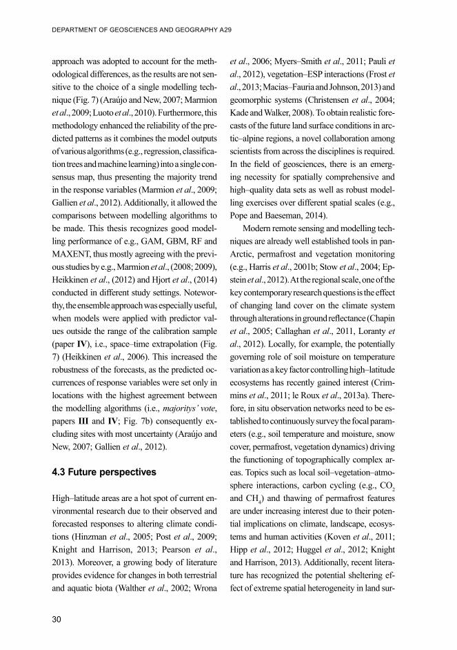
approach was adopted to account for the meth-odological differences, as the results are not sen-sitive to the choice of a single modelling tech-nique (Fig. 7) (Araújo and New, 2007; Marmion et al., 2009; Luoto et al., 2010). Furthermore, this methodology enhanced the reliability of the pre-dicted patterns as it combines the model outputs ofvariousalgorithms(e.g.,regression,classifica-tion trees and machine learning) into a single con-sensus map, thus presenting the majority trend in the response variables (Marmion et al., 2009; Gallien et al., 2012). Additionally, it allowed the comparisons between modelling algorithms to be made. This thesis recognizes good model-ling performance of e.g., GAM, GBM, RF and MAXENT, thus mostly agreeing with the previ-ous studies by e.g., Marmion et al., (2008; 2009), Heikkinen et al., (2012) and Hjort et al., (2014) conducted in different study settings. Notewor-thy, the ensemble approach was especially useful, when models were applied with predictor val-ues outside the range of the calibration sample (paper IV), i.e., space–time extrapolation (Fig. 7) (Heikkinen et al., 2006). This increased the robustness of the forecasts, as the predicted oc-currences of response variables were set only in locations with the highest agreement between the modelling algorithms (i.e., majoritys’ vote, papers III and IV; Fig. 7b) consequently ex-cluding sites with most uncertainty (Araújo and New, 2007; Gallien et al., 2012).

4.3 future perspectives

High–latitude areas are a hot spot of current en-vironmental research due to their observed and forecasted responses to altering climate condi-tions (Hinzman et al., 2005; Post et al., 2009; Knight and Harrison, 2013; Pearson et al., 2013).Moreover,agrowingbodyofliteratureprovides evidence for changes in both terrestrial and aquatic biota (Walther et al., 2002; Wrona

et al., 2006; Myers–Smith et al., 2011; Pauli et al., 2012), vegetation–ESP interactions (Frost et al.,2013;Macias–FauriaandJohnson,2013)andgeomorphic systems (Christensen et al., 2004; Kade and Walker, 2008). To obtain realistic fore-casts of the future land surface conditions in arc-tic–alpine regions, a novel collaboration among scientists from across the disciplines is required. In thefieldofgeosciences, there isanemerg-ing necessity for spatially comprehensive and high–quality data sets as well as robust model-ling exercises over different spatial scales (e.g., Pope and Baeseman, 2014).

Modern remote sensing and modelling tech-niques are already well established tools in pan-Arctic, permafrost and vegetation monitoring (e.g., Harris et al., 2001b; Stow et al., 2004; Ep-stein et al., 2012). At the regional scale, one of the key contemporary research questions is the effect of changing land cover on the climate system throughalterationsingroundreflectance(Chapinet al., 2005; Callaghan et al., 2011, Loranty et al., 2012). Locally, for example, the potentially governing role of soil moisture on temperature variation as a key factor controlling high–latitude ecosystems has recently gained interest (Crim-mins et al., 2011; le Roux et al.,2013a).There-fore, in situ observation networks need to be es-tablished to continuously survey the focal param-eters (e.g., soil temperature and moisture, snow cover, permafrost, vegetation dynamics) driving the functioning of topographically complex ar-eas. Topics such as local soil–vegetation–atmo-sphere interactions, carbon cycling (e.g., CO2

and CH4) and thawing of permafrost features are under increasing interest due to their poten-tial implications on climate, landscape, ecosys-tems and human activities (Koven et al., 2011; Hipp et al., 2012; Huggel et al., 2012; Knight andHarrison,2013).Additionally,recentlitera-ture has recognized the potential sheltering ef-fect of extreme spatial heterogeneity in land sur-

31

face conditions against climate change (Scherrer and Körner, 2011; Lenoir et al.,2013).AspaperIV implies, these pockets of suitable microcli-mates created by local conditions (Fig. 8) might be important for the preservation of both bio– and geodiversity under altering climatic conditions.

Even though statistical modelling is a valu-able framework for spatial analysis, mechanistic models describing, for example, heat and mass transfer processes might reduce uncertainties in predictions for future climate scenarios (Cramer et al., 2001; Fronzek et al., 2006). These pro-cess–based models, however, rely on heavy pa-rameterization and their spatial extent is limited (Lischke et al., 1998). Therefore, the next step in spatial modelling studies would be the incor-poration of statistical and mechanistic models (e.g., Shipley et al., 2006 and Bocedi et al., 2014 in an ecological context) for an improved land surface model. For example, the local develop-ment of cryoturbated soils could be described with a mechanistic model based on thermody-namics and hydrology, and further statistically transferred over broad high–latitude regions as

a function of e.g., land cover. However, the use of such approach will require co–operation be-tween physical geographers, ecologists, clima-tologists, hydrologists, geophysicists and soil sci-entists. Importantly, the spatial and holistic per-spective combined with strong methodological capabilities opens new possibilities for geogra-phers to be an integral part of future environ-mental research.

5 conclusions

By modelling multiple key high–latitude phe-nomena with modern statistical techniques and an ensemble approach, this thesis has provided new perspectives on process–environment rela-tionships across arctic–alpine landscapes. Sub-sequently,theanalyseshighlightedtheinfluenceof local conditions, for example topography and soil,thusreflectingthespatialheterogeneityofthese environments. Furthermore, this thesis pro-vided strong evidence for the argument that Earth surface processes pan–Arctic are potentially ex-

figure 8. The forecasted occurrence of nivation for increasing temperatures in relation to local topographical conditions (paper iV); A) elevation (m a.s.l.) and B) slope angle (in degrees). Dotted black line indicates the mean of predictions based on ten modelling techniques, while inner and outer shaded areas represent the 50th and 95th percentiles, respectively. The diagrams present how the distributional limits of nivation are first restricted to elevated and steep sites before the suitable climate conditions for the activity completely disappears from the study area.

32


tremely climatically sensitive.The main results and implications of this the-

sis can be summarized as follows:• The spatial modelling approach proved to be

an effective tool for investigating the struc-ture and functioning of high–latitude sys-tems. The spatial variation in temperature ex-tremes, ground thermal–hydrological condi-tions and ESPs were robustly modelled and predicted. Importantly, the analytical mod-elling tools help to conceptualize and struc-ture the complex and hierarchical process–environment relationships in arctic–alpine regions.

• The results underline the governing role of oceanic and topographical gradients as key meso–scale drivers of temperature variations in high–latitude region. Moreover, accurate temperature maps describing the meso–scale variation in extreme and mean temperature conditions were produced.

• Extreme variation in soil temperature and moisture was observed over short distanc-es,reflectingthestrongspatialheterogene-ity of thermal and hydrological conditions in these systems. While vegetation has an im-portant role in mediating soil temperatures andmoisturepatternsatfinespatialscaleinthe arctic–alpine system, topography and soil characteristicsrevealedtobethemostinflu-ential factors. However, when modeling soil temperature and moisture, vegetation proper-ties need to be explicitly considered.

• Themodelling ofESPswill benefit fromthe inclusion of local predictors, such as to-pography and soil characteristics, with in-creased transferability compared to climate–only models. This highlights the role of local factors determining the geomorphic activity patterns across arctic–alpine landscapes.

• ESPs are potentially extremely climatic sen-sitive.Theincreaseof2°Crelativetocur-

rent temperature conditions was projected to cause a near–complete loss of active ESPs in the arctic–alpine study area. As climate change proceeds, the suitable climatic spac-es for the occurrence of ESPs may global-ly shrink to a few topographically complex mountain areas.

• The methodology developed in this thesis can be used to produce novel datasets for the use of other disciplines, for example climatolo-gist, ecologist and geoscientist.

referencesAbiskoScientificResearchStation,2012.http://www.

polar.se/. (20.08.2012). Albrecht, J., Car, A., 1999. GIS analysis for scale–sen-

sitive environment modelling based on hierarchy theory. In: Dikau, R., Saurer, H. (Eds.), GIS for Earth Surface Systems. Gebrüder Borntraeger, Berlin,pp.1–23.

Allard, M. 1996. Geomorphological changes and per-mafrost dynamics: Key factors in changing arctic ecosystems. An example from Bylot Island, Nuna-vut, Canada. Geoscience Canada 23: 205–212.

Allouche, O., Tsoar, A., Kadmon, R. 2006. Assess-ing the accuracy of species distribution models: Prevalence, kappa and the true skill statistic (TSS).Journal of Applied Ecology 43:1223–1232.

Araújo, M.B., Whittaker, R.J., Ladle, R.J., Erhard, M. 2005. Reducing uncertainty in projections of ex-tinction risk from climate change. Global Ecology and Biogeography 14:529–538.

Araújo, M.B., Luoto, M. 2007. The importance of biotic interactions for modelling species distribu-tions under climate change. Global Ecology and Biogeography 16:743–753.

Araujo, M.B., New, M. 2007. Ensemble forecasting of species distributions. Trends in Ecology & Evolu-tion 22: 42–47.

Ballantyne, C.K., Matthews, J.A. 1982. The devel-opment of sorted circles on recently deglaciated terrain, Jotunheimen, Norway. Arctic, Antarctic and Alpine Research 14:341–354.

Barry, R.G., Chorley, R.J. 2009. Atmosphere, weather and climate. Routledge.

Bertoldi, G., Notarnicola, C., Leitinger, G., Endrizzi, S., Zebisch, M., Della Chiesa, S., Tappeiner, U. 2010. Topographical and ecohydrological controls on land surface temperature in an alpine catch-ment. Ecohydrology 3: 189–204.

Beven, K., Kirkby, M. 1979. A physically based vari-

33

able contributing area model of basin hydrology. Hydrological Sciences Bulletin. 24:43–69.

Billings,W.1973.Arcticandalpinevegetations:simi-larities, differences, and susceptibility to distur-bance. Bioscience 23: 697–704.

Billings, W. 1974. Adaptations and origins of alpine plants. Arctic, Antarctic and Alpine Research 6: 129–142.

Bocedi, G., Palmer, S.C., Pe’er, G., Heikkinen, R.K., Matsinos,Y.G.,Watts, K., Travis, J.M. 2014.RangeShifter: a platform for modelling spatial eco-evolutionary dynamics and species’ responses to environmental changes. Methods in Ecology and Evolution 5:388–396.

Boeckli, L., Brenning, A., Gruber, S., Noetzli, J. 2012. A statistical approach to modelling permafrost dis-tribution in the European Alps or similar mountain ranges. Cryosphere 6: 125–140.

Borcard, D., Legendre, P., Drapeau, P. 1992. Partialling Out the Spatial Component of Ecological Varia-tion. Ecology 73: 1045–1055.

Bosiö, J., Johansson, M., Callaghan, T.V., Johansen, B., Christensen, T.R. 2012. Future vegetation changes in thawing subarctic mires and impli-cations for greenhouse gas exchange–a regional assessment. Climate Change 115:379–398.

Bowman, W.D., Seastedt, T.R. 2001. Structure and function of an alpine ecosystem: Niwot Ridge, Colorado. Oxford University Press.

Breiman, L. 2001. Random forests. Machine learn-ing 45:5–32.

Broll, G., Tarnocai, C., Mueller, G. 1999. Interac-tions between vegetation, nutrients and moisture insoilsinthePangnirtungPassarea,BaffinIs-land, Canada. Permafrost Periglacial Processes 10: 265–277.

Brown, J., Ferrians, O.J.J., Heginbottom, J.A., Mel-nikov, E.S. 1998. Circum–arctic map of perma-frost and ground ice conditions. Boulder, Colo-rado USA: National Snow and Ice Data Center.

Bruun, H.H., Moen, J., Virtanen, R., Grytnes, J., Ok-sanen, L., Angerbjörn, A. 2006. Effects of altitude and topography on species richness of vascular plants, bryophytes and lichens in alpine commu-nities. Journal of Vegetation Science 17:37–46.

Cahoon, S.M., Sullivan, P.F., Shaver, G.R., Welker, J.M., Post, E. 2012. Interactions among shrub cover and the soil microclimate may determine future Arctic carbon budgets. Ecology Letters 15: 1415–1422.

Callaghan, T. V., Johansson, M., Key, J., Prowse, T., Ananicheva, M., Klepikov, A. 2011. Feedbacks and interactions: From the Arctic cryosphere to the climate system, Ambio 40 (S1): 75–86.

Carter, T.R., Porter, J.H., Parry, M.L. 1991. Climatic Warming and Crop Potential in Europe – Pros-pects and Uncertainties. Global Environmen-tal Change–Human and Policy Dimensions 1: 291–312.

Chapin,F.S.1983.DirectandIndirectEffectsofTem-perature on Arctic Plants. Polar Biology 2: 47–52.

Chapin, F.S., Sturm, M., Serreze, M.C., McFadden, J.P., Key, J.R., Lloyd, A.H., McGuire, A.D., Rupp, T.S., Lynch, A.H., Schimel, J.P., Beringer, J., Chapman, W.L., Epstein, H.E., Euskirchen, E.S., Hinzman, L.D., Jia, G., Ping, C.L., Tape, K.D., Thompson, C.D.C., Walker, D.A., Welker, J.M. 2005. Role of land–surface changes in Arctic summer warming. Science 310: 657–660.

Christensen, T.R., Johansson, T.R., Akerman, H.J., Mastepanov, M., Malmer, N., Friborg, T., Crill, P., Svensson, B.H. 2004. Thawing sub–arctic per-mafrost: Effects on vegetation and methane emis-sions. Geophysical Research Letters 31: L04501.

Christiansen, H.H., Etzelmüller, B., Isaksen, K., Ju-liussen, H., Farbrot, H., Humlum, O., Johansson, M., Ingeman-Nielsen, T., Kristensen, L., Hjort, J. 2010. The thermal state of permafrost in the nordic area during the international polar year 2007–2009. Permafrost and Periglacial Pro-cesses 21:156-181.

Cramer, W., Bondeau, A., Woodward, F.I., Prentice, I.C., Betts, R.A., Brovkin, V., Cox, P.M., Fisher, V., Foley, J.A., Friend, A.D. 2001. Global response of terrestrial ecosystem structure and function to CO2 and climate change: results from six dynamic global vegetation models. Global Change Biol-ogy 7:357–373.

Crimmins, S.M., Dobrowski, S.Z., Greenberg, J.A., Abatzoglou, J.T., Mynsberge, A.R. 2011. Changes in climatic water balance drive downhill shifts in plant species’ optimum elevations. Science 331: 324–327.

Daanen, R.P., Misra, D., Epstein, H., Walker, D., Ro-manovsky, V. 2008. Simulating nonsorted circle development in arctic tundra ecosystems. Journal of Geophysical Research: Biogeosciences (2005–2012) 113:G3.

Daly, C. 2006. Guidelines for assessing the suitability of spatial climate data sets. International Journal of Climatology 26: 707–721.

Dormann, C.F., McPherson, J.M., Araujo, M.B., Bivand, R., Bolliger, J., Carl, G., Davies, R.G., Hirzel, A., Jetz, W., Kissling, W.D., Kuehn, I., Ohlemueller, R., Peres–Neto, P.R., Reineking, B., Schroeder, B., Schurr, F.M., Wilson, R. 2007. Methods to account for spatial autocorrelation in the analysis of species distributional data: a review. Ecography 30: 609–628.

Dormann, C.F., Elith, J., Bacher, S., Buchmann, C., Carl, G., Carre, G., Garcia Marquez, J.R., Gruber, B., Lafourcade, B., Leitao, P.J., Muenkemueller, T., McClean, C., Osborne, P.E., Reineking, B., Schroeder, B., Skidmore, A.K., Zurell, D., Laut-enbach,S.2013.Collinearity:areviewofmethodsto deal with it and a simulation study evaluating their performance. Ecography 36: 27–46.

Ehrenfeld, J., Ravit, B., Elgersma, K. 2005. Feedback

34


in the plant–soil system. AnnualReview of Envi-ronment and Resources 30: 75–115.

Elith, J., Leathwick, J.R., Hastie, T. 2008. A work-ing guide to boosted regression trees. Journal of Animal Ecology 77:802–813.

Epstein, H.E., Raynolds, M.K., Walker, D.A., Bhatt, U.S., Tucker, C.J., Pinzon, J.E. 2012. Dynamics of aboveground phytomass of the circumpolar Arctic tundra during the past three decades. Environmen-tal Research Letters 7: 015506.

Esri, 2013. ArcScripts. www.arcsripts.esri.com. (23.9.2013).

Etzelmüller,B.2013.RecentAdvancesinMountainPermafrost Research. Permafrost and Periglacial Processes 24: 99–107.

European Environment Agency, 2012. Corine Land Cover 2006 raster data.

Farbrot, H., Isaksen, K., Etzelmüller, B., Gisnas, K. 2013.GroundThermalRegimeandPermafrostDistribution under a Changing Climate in North-ern Norway. Permafrost Periglacial Processes 24: 20–38.

Fielding, A.H., Bell, J.F. 1997. A review of methods for the assessment of prediction errors in conser-vation presence/absence models. Environmental Conservation 24:38–49.

Finnish Environmental Institute, 2006. Corine Land Cover 2006. (28.1.2014).

Fountain, A.G., Campbell, J.L., Schuur, E.A.G., Stam-merjohn, S.E., Williams, M.W., Ducklow, H.W. 2012. The Disappearing Cryosphere: Impacts and Ecosystem Responses to Rapid Cryosphere Loss. Bioscience 62: 405–415.

French, H.M. 2007. The periglacial environment. John Wiley & Sons, Chichester.

Fronzek, S., Luoto, M., Carter, T.R. 2006. Potential effect of climate change on the distribution of palsa mires in subarctic Fennoscandia. Climate Research 32: 1–12.

Fronzek, S., Carter, T.R., Luoto, M. 2011. Evaluating sources of uncertainty in modelling the impact of probabilistic climate change on sub–arctic palsa mires. Natural Hazards and Earth System Sci-ences 11: 2981–2995.

Frost, G.V., Epstein, H.E., Walker, D.A., Matyshak, G., Ermokhina,K.2013.Patterned–groundfacilitatesshrub expansion in Low Arctic tundra. Environ-mental Research Letters 8:015035.

Gallien, L., Douzet, R., Pratte, S., Zimmermann, N.E., Thuiller, W. 2012. Invasive species distribution models – how violating the equilibrium assump-tion can create new insights. Global Ecology and Biogeography 21:1126–1136.

Geological Survey of Finland, 2010. Digital soil data-base. Geological Survey of Finland: Espoo.

Graham,E.A.,Rundel,P.W.,Kaiser,W.,Lam,Y.,Stealey,M.,Yuen,E.M.2012.Fine–scalepat-terns of soil and plant surface temperatures in an

alpine fellfieldhabitat,WhiteMountains,Cali-fornia. Arctic, Antarctic, and Alpine Research 44: 288–295.

Graham,M.H.2003.Confrontingmulticollinearityin ecological multiple regression. Ecology 84: 2809–2815.

Greenland, D., Losleben, M. 2001. Climate. In: Bow-man, W.D., Seastedt, T.R. (Eds.), Structure and function of Alpine ecosystem. Oxfrod University Press, Oxford.

Guisan, A., Zimmermann, N.E. 2000. Predictive habitat distribution models in ecology. Ecologi-cal Modelling 135: 147–186.

Guisan, A., Thuiller, W. 2005. Predicting species distri-bution: offering more than simple habitat models. Ecology Letters 8:993–1009.

Harris, C., Rea, B., Davies, M. 2001a. Scaled physi-cal modelling of mass movement processes on thawing slopes. Permafrost Periglacial Processes 12:125–135.

Harris, C., Haeberli, W., Vonder Mühll, D., King, L. 2001b. Permafrost monitoring in the high moun-tains of Europe: the PACE project in its global con-text. Permafrost Periglacial Processes 12:3–11.

Harris, C., Smith, J.S., Davies, M.C.R., Rea, B. 2008. An investigation of periglacial slope stability in relation to soil properties based on physical model-ling in the geotechnical centrifuge. Geomorphol-ogy 93:437–459.

Heikkinen, R.K., Luoto, M., Araujo, M.B., Virkkala, R., Thuiller, W., Sykes, M.T. 2006. Methods and uncertainties in bioclimatic envelope modelling under climate change. Progress in Physical Ge-ography 30: 751–777.

Heikkinen, R.K., Marmion, M., Luoto, M. 2012. Does the interpolation accuracy of species distribution models come at the expense of transferability? Ecography 35: 276–288.

Hinzman, L.D., Bettez, N.D., Bolton, W.R., Chap-in,F.S.,Dyurgerov,M.B.,Fastie,C.L.,Griffith,B., Hollister, R.D., Hope, A., Huntington, H.P. 2005. Evidence and implications of recent climate change in northern Alaska and other arctic regions. Climate Change 72: 251–298.

Hipp, T., Etzelmuller, B., Farbrot, H., Schuler, T.V., Westermann, S. 2012. Modelling borehole tem-peratures in Southern Norway – insights into permafrost dynamics during the 20th and 21st century. Cryosphere 6:553–571.

Hjort, J., Luoto, M., Seppalä, M. 2007. Landscape scale determinants of periglacial features in sub-arctic Finland: A grid–based modelling approach. Permafrost Periglacial Processes 18: 115–127.

Hjort, J., Luoto, M. 2009. Interaction of geomorphic and ecologic features across altitudinal zones in a subarctic landscape. Geomorphology 112: 324–333.

Hjort, J., Luoto, M. 2011. Novel theoretical insights

35

into geomorphic process–environment relation-ships using simulated response curves. Earth Surface Processes and Landforms 36:363–371.

Hjort,J.,Luoto,M.2013.Statisticalmethodsforgeo-morphic distribution modeling. Treatise on Geo-morphology, Shroder J, Jr (ed). Academic Press: SanDiego,59–73.

Hjort, J., Ujanen, J., Parviainen, M., Tolgensbakk, J., Etzelmüller, B. 2014. Transferability of geomor-phological distribution models: Evaluation using solifluction features insubarcticandArctic re-gions. Geomorphology 204: 165–176.

Hjort, J. 2014. Which environmental factors determine recentcryoturbationandsolifluctionactivityinasubarctic landscape? A comparison between ac-tive and inactive features. Permafrost and Peri-glacial Processes 25:136–143.

Huggel, C., Clague, J.J., Korup, O. 2012. Is climate change responsible for changing landslide activity in high mountains? Earth Surface Processes and Landforms 37: 77–91.

IPCC,2013.SummaryforPolicymakers.In:Stocker,T.F., Qin, D., Plattner, G.K., Tignor, M., Allen, S.K.,Boschung,J.,Nauels,A.,Xia,Y.,Bex,V.,Midgley, P.M. (Eds.), Climate Change 2013: The Physical Science Basis. Contribution of Working Group I to the Fifth Assessment Report of the Intergovernmental Panel on Climate Change. Cambridge University Press, Cambridge, United KingdomandNewYork,NY,USA.

Isard,S.A.1986.FactorsInfluencingSoil–Moistureand Plant Community Distribution on Niwot Ridge, Front Range, Colorado, Usa. Arctic, Ant-arctic, and Alpine Research 18:83–96.

Johnson, P.L., Billings, W.D. 1962. The Alpine Veg-etation of the Beartooth Plateau in Relation to Cryopedogenic Processes and Patterns. Ecologi-cal Monographs 32:105–135.

Jylhä, K., Ruosteenoja, K., Räisänen, J., Venäläinen, A., Tuomenvirta, H., Ruokolainen, L., Saku, S., Seitola, T. 2009. Arvioita Suomen muuttuvasta ilmastosta sopeutumistutkimuksia varten. Finn-ish Meteorological Institute, Helsinki, Finland. (In Finnish).

Kade, A., Walker, D.A. 2008. Experimental altera-tion of vegetation on nonsorted circles: Effects on cryogenic activity and implications for climate change in the arctic. Arctic, Antarctic, and Alpine Research 40:96–103.

Kivinen, S., Kaarlejärvi, E., Jylhä, K., Räisänen, J. 2012. Spatiotemporal distribution of threatened high–latitude snowbed and snow patch habitats in warming climate. Environmental Research Let-ters 7:034024.

Knight,J.,Harrison,S.2013.Theimpactsofclimatechange on terrestrial Earth surface systems. Nature Climate Change 3: 24–29.

Koven, C.D., Ringeval, B., Friedlingstein, P., Ciais, P., Cadule, P., Khvorostyanov, D., Krinner, G., Tar-

nocai, C. 2011. Permafrost carbon–climate feed-backs accelerate global warming. Proceedings of the National Academy of Sciences of the United States of America 108: 14769–14774.

Laitakari, I. 1998. Peruskallion myöhäiset kehitysvai-heet – miljardi rauhallista vuotta. In: Lehtinen, M., Nurmi, P., Rämö, T. (Eds.), Suomen kallioperä – 3000 vuosimiljoonaa. The Geological Society of Finland,pp.309–325.(InFinnish).

LandSurveyofFinland,2013.MapSite.www.kans-alaisen.karttapaikka.fi.(19.9.2013).

Legates, D.R., Mahmood, R., Levia, D.F., DeLiberty, T.L., Quiring, S.M., Houser, C., Nelson, F.E. 2011. Soil moisture: A central and unifying theme in physical geography. Progress in Physical Geog-raphy 35: 65–86.

Legendre, P., Dale, M.R.T., Fortin, M.J., Gurevitch, J., Hohn, M., Myers, D. 2002. The consequences of spatial structure for the design and analysis of ecologicalfieldsurveys.Ecography 25: 601–615.

Lenoir, J., Graae, B.J., Aarrestad, P.A., Alsos, I.G., Armbruster, W.S., Austrheim, G., Bergendorff, C., Birks,H.J.B.,Bråthen,K.A.,Brunet,J.2013.Lo-cal temperatures inferred from plant communities suggest strong spatial buffering of climate warm-ing across Northern Europe. Global Change Biol-ogy 19: 1470–1481.

Lischke, H., Guisan, A., Fischlin, A., Williams, J., Bugmann, H. 1998. Vegetation responses to cli-mate change in the Alps: modeling studies. MIT Press, Boston, Massachusetts.

Litaor, M., Williams, M., Seastedt, T. 2008. Topo-graphic controls on snow distribution, soil mois-ture, and species diversity of herbaceous alpine vegetation, Niwot Ridge, Colorado. Journal of Geophysical Research: Biogeosciences 113: G2.

Lloyd, J., Taylor, J.A. 1994. On the Temperature De-pendence of Soil Respiration. Functional Ecology 8:315–323.

Loranty, M.M., Goetz, S.J. 2012. Shrub expansion and climate feedbacks in Arctic tundra. Environmental Research Letters 7: 011005.

Luoto,M.,Seppalä,M.2003.Thermokarstpondsasindicators of the former distribution of palsas in Finnish lapland. Permafrost Periglacial Processes 14: 19–27.

Luoto, M., Fronzek, S., Zuidhoff, F.S. 2004. Spatial modelling of palsa mires in relation to climate in northern Europe. Earth Surface Processes and Landforms 29:1373–1387.

Luoto, M., Hjort, J., 2005. Evaluation of current statis-tical approaches for predictive geomorphological mapping. Geomorphology 67:299–315.

Luoto, M., Marmion, M., Hjort, J. 2010. Assessing spatial uncertainty in predictive geomorphological mapping: A multi–modelling approach. Computer & Geosciences 36:355–361.

Mac Nally, R. 2002. Multiple regression and infer-ence in ecology and conservation biology: fur-

36


ther comments on identifying important predic-tor variables. Biodiversity and Conservation 11: 1397–1401.

Macias–Fauria,M.,Johnson,E.A.2013.Warming–induced upslope advance of subalpine forest is severely limited by geomorphic processes. Pro-ceedings of the National Academy of Sciences of the United States of America 110: 8117–8122.

Malanson, G.P., Bengtson, L.E., Fagre, D.B. 2012. Geomorphic Determinants of Species Compo-sition of Alpine Tundra, Glacier National Park, U.S.A. Arctic, Antarctic, and Alpine Research 44: 197–209.

Marchand, F.L., Kockelbergh, F., van de Vijver, B., Beyens, L., Nijs, I. 2006. Are heat and cold re-sistance of arctic species affected by successive extreme temperature events? New Phytologist 170:291–300.

Marmion, M., Hjort, J., Thuiller, W., Luoto, M. 2008. A comparison of predictive methods in modelling the distribution of periglacial landforms in Finnish Lapland. Earth Surface Processes and Landforms 33: 2241–2254.

Marmion, M., Hjort, J., Thuiller, W., Luoto, M. 2009. Statistical consensus methods for improving pre-dictive geomorphology maps. Computers & Geo-sciences 35: 615–625.

Matsuoka,N.2001.Solifluctionrates,processesandlandforms: a global review. Earth–Science Re-views 55:107–134.

Matsuoka, N. 2005. Temporal and spatial variations in periglacial soil movements on alpine crest slopes. Earth Surface Processes and Landforms 30: 41–58.

Matthews, J.A., Shakesby, R.A., Berrisford, M.S., McEwen, L.J. 1998. Periglacial patterned ground on the Styggedalsbreen glacier foreland, Jotun-heimen, southern Norway: Micro–topographic, paraglacial and geoecological controls. Perma-frost Periglacial Processes 9: 147–166.

McCune, B., Keon, D. 2002. Equations for potential annual direct incident radiation and heat load. Journal of Vegetation Science 13:603–606.

Meehl, G.A., Covey, C., Delworth, T., Latif, M., McA-vaney, B., Mitchell, J.F.B., Stouffer, R.J., Taylor, K.E.2007.TheWCRPCMIP3multimodeldata-set – A new era in climate change research. Bul-letin of the American Meteorological Society 88: 1383–1394.

Mod, H.K., Roux, P.C., Luoto, M. 2014. Outcomes of biotic interactions are dependent on multiple environmental variables. Journal of Vegetation Science 25,1024–1032.

Myers–Smith, I.H., Forbes, B.C., Wilmking, M., Hal-linger, M., Lantz, T., Blok, D., Tape, K.D., Ma-cias–Fauria, M., Sass–Klaassen, U., Lévesque, E. 2011. Shrub expansion in tundra ecosystems: dynamics, impacts and research priorities. Envi-

ronmental Research Letters 6: 045509. Nakićenović,N.,Joseph,A.,Gerald,D.,deVries,B.,

Fenhann,J.,Gaffin,S.,Gregory,K.,Grubler,A.,Jung, T.J., Kram, T., La Rovere, E.L., Michae-lis, L., Mori, S., Morita, T., Pepper, W., Pitcher, H.M., Price, L., Riahi, K., Roehrl, A., Rogner, H.H., Sankovski, A., Schlesinger, M., Shukla, P., Smith, S.J., Swart, R., van Rooijen, S., Victor, N., Dadi, Z. 2000. Special Report on Emission Sce-narios: a Special Report of Working Group III of the Intergovernmental Panel on Climate Change.

NASA Land Processes Distributed Active Archive Center(LPDAAC),2013.ASTERDEM.https://lpdaac.usgs.gov/data_access.(13.03.2014).

Norwegian Meteorological Institute, 2012. eKlima. https://eklima.met.no/. (20.08.2012).

Oksanen, J., Sarjakoski, T. 2005. Error propagation analysis of DEM–based drainage basin delinea-tion. International Journal of Remote Sensing 26: 3085–3102.

Parmesan, C., Root, T.L., Willig, M.R. 2000. Impacts of extreme weather and climate on terrestrial biota. Bulletin of American Meteorological Society 81: 443–450.

Pauli, H., Gottfried, M., Dullinger, S., Abdaladze, O., Akhalkatsi, M., Benito Alonso, J.L., Coldea, G., Dick, J., Erschbamer, B., Fernandez Calzado, R., Ghosn, D., Holten, J.I., Kanka, R., Kazakis, G., Kollar, J., Larsson, P., Moiseev, P., Moiseev, D., Molau, U., Molero Mesa, J., Nagy, L., Pelino, G., Puscas, M., Rossi, G., Stanisci, A., Syverhuset, A.O., Theurillat, J.P., Tomaselli, M., Unterlug-gauer, P., Villar, L., Vittoz, P., Grabherr, G. 2012. Recent plant diversity changes on Europe’s moun-tain summits. Science 336:353–355.

Payette, S., Delwaide, A., Caccianiga, M., Beauche-min, M. 2004. Accelerated thawing of subarctic peatland permafrost over the last 50 years. Geo-physical Research Letters 31: L18208.

Pearson, R.G., Dawson,T.P. 2003. Predicting theimpacts of climate change on the distribution of species: are bioclimate envelope models useful? Global Ecology and Biogeography 12:361–371.

Pearson, R.G., Dawson, T.P., Liu, C. 2004. Modelling species distributions in Britain: a hierarchical inte-gration of climate and land-cover data. Ecography 27: 285–298.

Pearson, R.G., Phillips, S.J., Loranty, M.M., Beck, P.S., Damoulas, T., Knight, S.J., Goetz, S.J. 2013.ShiftsinArcticvegetationandassociatedfeedbacks under climate change. Nature Climate Change 3:673–677.

Phillips,J.D.2003.Sourcesofnonlinearityandcom-plexity in geomorphic systems. Progress in Physi-cal Geography 27:1–23.

Pike,G.,Pepin,N.,Schaefer,M.2013.Highlatitudelocal scale temperature complexity: the example of Kevo Valley, Finnish Lapland. International

37

Journal of Climatology 33: 2050–2067. Pope, A., Baeseman, J. 2014. The Cryosphere in a

Changing Climate. Eos, Transactions American Geophysical Union 95: 128–128.

Post, E., Forchhammer, M.C., Bret–Harte, M.S., Cal-laghan, T.V., Christensen, T.R., Elberling, B., Fox, A.D., Gilg, O., Hik, D.S., Hoye, T.T., Ims, R.A., Jeppesen, E., Klein, D.R., Madsen, J., McGuire, A.D., Rysgaard, S., Schindler, D.E., Stirling, I., Tamstorf, M.P., Tyler, N.J.C., van der Wal, R., Welker, J., Wookey, P.A., Schmidt, N.M., Aastrup, P. 2009. Ecological Dynamics Across the Arctic Associated with Recent Climate Change. Science 325:1355–1358.

Potter,K.A.,Woods,H.A.,Pincebourde,S.2013.Mi-croclimatic challenges in global change biology. Global Change Biology 19:2932–2939.

R Development Core Team, 2011. R: A language and environment for statistical computing. R Founda-tion for Statistical Computing.

Ridefelt, H., Etzelmuller, B., Boelhouwers, J. 2010. SpatialAnalysisofSolifluctionLandformsandProcess Rates in the Abisko Mountains, North-ern Sweden. Permafrost Periglacial Processes 21: 241–255.

Rolland,C.2003.Spatialandseasonalvariationsofairtemperature lapse rates in Alpine regions. Journal of Climate 16:1032–1046.

leRoux,P.C.,Aalto,J.,Luoto,M.2013a.Soilmois-ture’s underestimated role in climate change im-pact modelling in low–energy systems. Global Change Biology 19: 2965–2975.

leRoux,P.C.,Virtanen,R.,Luoto,M.2013b.Geomor-phological disturbance is necessary for predicting fine–scalespeciesdistributions.Ecography 36: 800–808.

le Roux, P.C., Luoto, M. 2014. Earth surface processes drive the richness, composition and occurrence of plant species in an arctic–alpine environment. Journal of Vegetation Science 25: 45–54.

le Roux, P.C., Pellissier, L., Wisz, M.S., Luoto, M. 2014. Incorporating dominant species as proxies for biotic interactions strengthens plant commu-nity models. Journal of Ecology 102: 767–775.

Saito,M.,Kato,T.,Tang,Y.2009.Temperaturecon-trols ecosystem CO2 exchange of an alpine mead-ow on the northeastern Tibetan Plateau. Global Change Biology 15: 221–228.

Scherrer, D., Körner, C. 2010. Infra–red thermom-etry of alpine landscapes challenges climatic warming projections. Global Change Biology 16:2602–2613.

Scherrer, D., Körner, C. 2011. Topographically con-trolled thermal–habitat differentiation buffers alpine plant diversity against climate warming. Journal of Biogeography 38: 406–416.

Scherrer, D., Schmid, S., Körner, C. 2011. Elevational species shifts in a warmer climate are overesti-mated when based on weather station data. Inter-

national Journal of Biometeorology 55: 645–654. Schumm, S.A. 1979. Geomorphic Thresholds: The

Concept and Its Applications. Transactions of the Institute of British Geographers 4: 485–515.

Seppälä, M. 1986. The origin of palsas. Geografiska Annaler 68A: 141–147.

Serreze, M., Walsh, J., Chapin Iii, F., Osterkamp, T., Dyurgerov, M., Romanovsky, V., Oechel, W., Morison, J., Zhang, T., Barry, R. 2000. Observa-tional evidence of recent change in the northern high–latitude environment. Climate Change 46: 159–207.

Shipley, B., Vile, D., Garnier, E. 2006. From plant traits to plant communities: A statistical mechanistic ap-proach to biodiversity. Science 314: 812–814.

Skov, F., Svenning, J.C. 2004. Potential impact of cli-matic change on the distribution of forest herbs in Europe. Ecography 27:366–380.

Sormunen, H., Virtanen, R., Luoto, M. 2011. Inclu-sion of local environmental conditions alters high–latitude vegetation change predictions based on bioclimatic models. Polar Biology 34:883–897.

Stallins, J.A. 2006. Geomorphology and ecology: uni-fying themes for complex systems in biogeomor-phology. Geomorphology 77: 207–216.

Starr, G., Oberbauer, S.F., Ahlquist, L.E. 2008. The photosynthetic response of Alaskan tundra plants to increased season length and soil warming. Arc-tic, Antarctic, and Alpine Research 40: 181–191.

Stow, D.A., Hope, A., McGuire, D., Verbyla, D., Gamon, J., Huemmrich, F., Houston, S., Racine, C., Sturm, M., Tape, K. 2004. Remote sensing of vegetation and land–cover change in Arctic Tun-dra Ecosystems. Remote Sensing of Environment 89:281–308.

Sturm, M., Racine, C., Tape, K. 2001. Increasing shrub abundance in the Arctic. Nature 411: 546–547.

Swanson, F., Kratz, T., Caine, N., Woodmansee, R. 1988. Landform effects on ecosystem patterns and processes. BioScience 38: 92–98.

Swedish Meteorological and Hydrological Institute, 2012. Smhi. http://www.smhi.se/. (20.08.2012).

Swets, J.A. 1988. Measuring the accuracy of diagnos-tic systems. Science 240:1285–1293.

Takahashi, K. 2005. Seasonal changes in soil tempera-ture on an upper windy ridge and lower leeward slope in Pinus Pumila scrub on Mt. Shogigashira, central Japan. Polar Bioscince 18: 82–89.

Tape, K., Sturm, M., Racine, C. 2006. The evidence for shrub expansion in Northern Alaska and the Pan–Arctic. Global Change Biology 12: 686–702.

Thorn,C.E.1979.GroundTemperaturesandSurficialTransport in Colluvium during Snowpatch Melt-out – Colorado Front Range. Arctic, Antarctic, and Alpine Research 11: 41–52.

Thorn, C.E., Hall, K. 2002. Nivation and cryoplana-tion: the case for scrutiny and integration. Progress in Physical Geography 26:533–550.

Thuiller, W. 2004. Patterns and uncertainties of spe-

38


cies’ range shifts under climate change. Global Change Biology 10: 2020–2027.

Thuiller,W.,Georges,D.,Engler,R.2013.biomod2: Ensemble platform for species distribution model-ing. R package version 2.1.15.

Tikkanen, M. 2005. Climate. In: Seppälä, M. (Ed.), The physical geography of Fennoscandia. Oxford University Press, Oxford.

USGS, 2004. Shuttle radar topography mission. U.S. Department of the Interior.

Van Houwelingen, J., Le Cessie, S. 1990. Predic-tive value of statistical models. Stat.Med. 9(11), 1303–1325.VanNiel,K.P.,Austin,M.P.,2007.Predictive vegetation modeling for conservation: Impact of error propagation from digital eleva-tion data. Ecological Applications 17: 266–280.

Venables, W.N., Ripley, B.D. 2002. Modern Applied Statistics with S. Springer, Berlin.

Virtanen, R., Luoto, M., Rama, T., Mikkola, K., Hjort, J., Grytnes, J., Birks, H.J.B. 2010. Recent vegeta-tion changes at the high–latitude tree line ecotone are controlled by geomorphological disturbance, productivity and diversity. Global Ecology and Biogeography 19: 810–821.

Vliet-Lanoë, V. 1991. Differential frost heave, load casting and convection: converging mechanisms; a discussion of the origin of cryoturbations. Per-mafrost Periglacial Processes 2:123–139.

Walsh, S.J., Butler, D.R., Malanson, G.P. 1998. An overview of scale, pattern, process relationships in geomorphology: a remote sensing and GIS per-spective. Geomorphology 21:183–205.

Walther, G., Post, E., Convey, P., Menzel, A., Parme-san, C., Beebee, T.J., Fromentin, J., Hoegh–Guld-berg, O., Bairlein, F. 2002. Ecological responses to recent climate change. Nature 416:389–395.

Washburn, A.L. 1979. Geocryology – a survey of periglacial processes and environments. Arnold, London.

Wrona, F.J., Prowse, T.D., Reist, J.D., Hobbie, J.E., Lévesque, L.M., Vincent, W.F. 2006. Climate change effects on aquatic biota, ecosystem struc-ture and function. Ambio 35:359–369.

Wundram,D.,Pape,R.,Löffler,J.2010.Alpinesoiltemperature variability at multiple scales. Arctic, Antarctic, and Alpine Research 42: 117–128.

Yang,Z.,Hanna,E.,Callaghan,T.V.2011.Modellingsurface–air–temperature variation over complex terrain around Abisko, Swedish Lapland: uncer-tainties of measurements and models at different scales. Geografiska Annaler 93A: 89–112.

Zimmermann,N.E.,Yoccoz,N.G.,Edwards,T.C.,Meier, E.S., Thuiller, W., Guisan, A., Schmatz, D.R., Pearman, P.B. 2009. Climatic extremes improve predictions of spatial patterns of tree species. Proceedings of the National Academy of Sciences 106 (S2):19723–19728.

errata

paper ii:

Page 4, in the caption of Figure 2 is written “… (D) peat depth … ”. It should be changed to “… (D) soil depth…”.

paper iii:

The citation “Hjort and Luoto, 2010” should be changed to:

“Hjort and Luoto, 2011”.

Similarly in the reference list, “Hjort J, Luoto M. 2010. Novel theoretical insights into geomorphicprocess–environment relationship using simulat-ed response curves.Earth Surface Processes and Landforms35:363–371.”shouldbechangedto: “Hjort J, Luoto M. 2011. Novel theoretical in-sights into geomorphic process–environment re-lationship using simulated response curves. Earth SurfaceProcessesandLandforms35:363–371.”

Documents

New perspectives on climate, Earth surface processes and