1 | P a g e

New Projections of Changing Heavy Precipitation for the City of Everett

Future storm projected by the regional climate model used in this study (Source: Eric Salathé)

Prepared by

Guillaume Mauger, UW Climate Impacts Group

Jason Won, UW Climate Impacts Group

Katherine Hegewisch, U. Idaho Department of Geography

Cary Lynch, Joint Global Change Research Institute

29 December 2017

2 | P a g e

Contents

1 Acknowledgements ................................................................................................................. 3

2 Report Updates........................................................................................................................ 4

3 Purpose..................................................................................................................................... 5

4 Background ............................................................................................................................. 6

5 Data .......................................................................................................................................... 7

5.1 Global Climate Model (GCM) Scenarios ........................................................................ 7

5.2 Regional Climate Model Simulations .............................................................................. 8

5.3 Observations .................................................................................................................... 9

6 Post-Processing ...................................................................................................................... 12

6.1 WRF data extraction ...................................................................................................... 12

6.2 Bias Correction .............................................................................................................. 12

6.3 Summary Statistics......................................................................................................... 14

6.4 Extreme Value Analysis ................................................................................................ 15

7 Results .................................................................................................................................... 16

7.1 Data Structure ................................................................................................................ 17

7.2 Summary: Projected Changes in 1-hour Precipitation Extremes ................................... 18

8 References .............................................................................................................................. 21

9 Appendix: Email description of data modifications to Silver Lake Gauge ..................... 23

3 | P a g e

1 Acknowledgements

The authors would like to thank Raquel Lorente Plazas and Rick Steed for their help in producing the

WRF simulations used in this report, as well as Cliff Mass for his generous donation of computing

resources. Robert Norheim produced the interactive online visualizations using Tableau. This project was

funded by the City of Everett, and was made possible by leveraged funding from the King County

Department of Natural Resources and Parks and the Washington State Department of Ecology.

Recommended citation format: Mauger, G.S., J.S. Won, K. Hegewisch, C. Lynch, 2017. New

Projections of Changing Heavy Preicpitation for the City of Everett. Report prepared for the City of

Everett. Climate Impacts Group, University of Washington, Seattle.

4 | P a g e

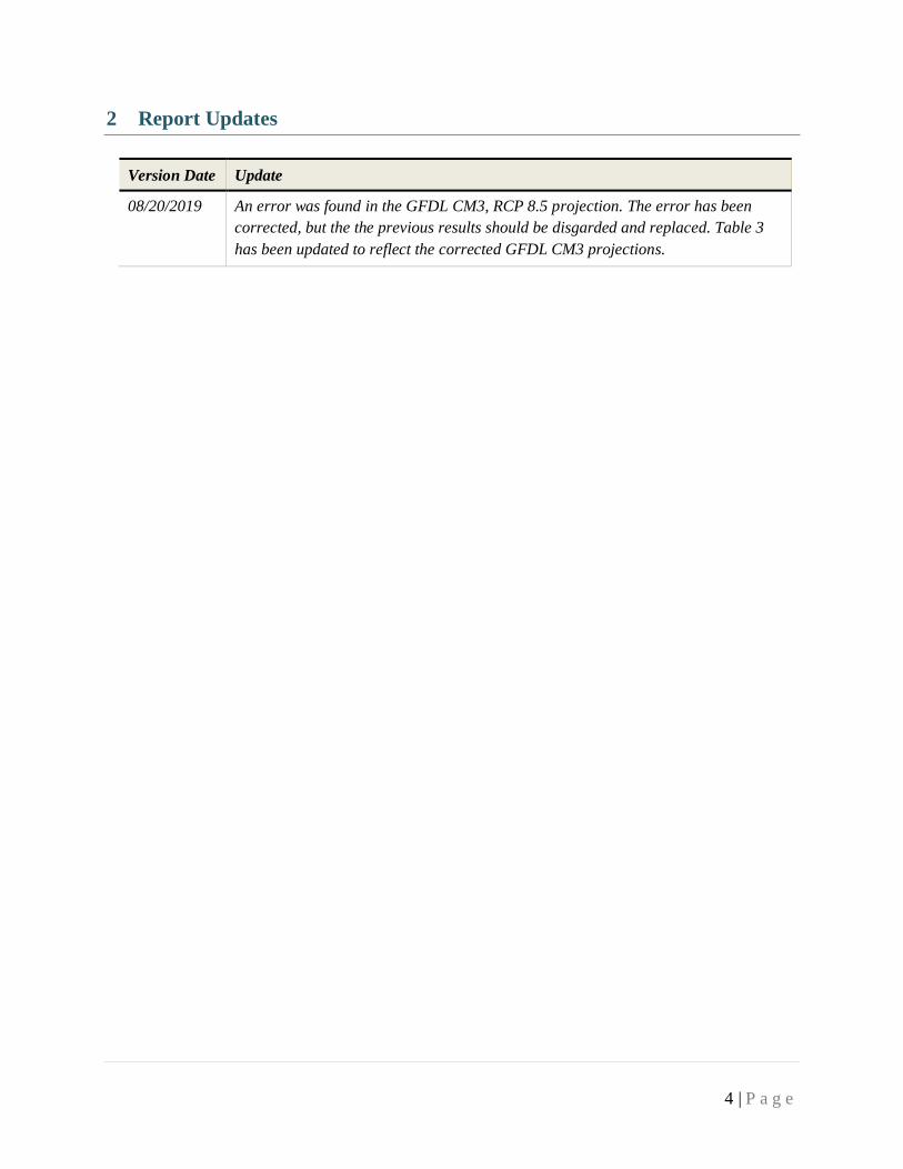
2 Report Updates

Version Date Update

08/20/2019 An error was found in the GFDL CM3, RCP 8.5 projection. The error has been

corrected, but the the previous results should be disgarded and replaced. Table 3

has been updated to reflect the corrected GFDL CM3 projections.

5 | P a g e

3 Purpose

The purpose of this project was to use new regional climate model simulations to develop

stormwater-relevant projections that are specific to the City of Everett.

The specific objectives of this work were to:

1. Produce hourly time series estimates of precipitation intensity for two regional model

simulations for specific locations of interest to city staff.

2. Develop estimates of the change in the intensity, duration, and frequency of heavy rain

events for the City of Everett

3. Create a set of summary products documenting the methodology and results.

This report describes the methods and products developed as part of the study, along with a brief

description of the results.

6 | P a g e

4 Background

Changes in the intensity, duration, and frequency of precipitation may negatively affect

stormwater facilities, exacerbate landslide and urban flood risk, and lead to other public safety

and water quality concerns. Recent research has shown that heavy rain events are projected to

become more intense with climate change (e.g., Warner et al. 2015, Trenberth 2011). This has

altered the calculus regarding climate change impacts in the Pacific Northwest, since previous

research suggested very little change in precipitation for the region. This is in part due to new

methods of “downscaling” the large-scale changes projected by global climate models (GCMs)

to smaller-scale changes of relevance to impacts assessment. Studies have shown that a physics-

based approach (“dynamical downscaling”), is needed to capture changes in precipitation

extremes and the associated impacts (Salathé et al. 2014). Previous approaches relied primarily

on an empirical approach (“statistical downscaling”), which does not provide reliable estimates

of changes in extremes. In dynamical downscaling, a regional climate model is used to simulate

local-scale changes in climate, leading to a better representation of changes in the physical

processes at these scales. This distinction is particularly important for precipitation, since

dynamical downscaling can explicitly represent the interactions of weather systems with the

complex terrain of the Pacific Northwest.

In 2015, King County awarded funding to the UW Climate Impacts Group (CIG) to develop new

regional climate model simulations of changing precipitation. The City of Everett currently uses

a set of climate projections showing a 9% increase in winter precipitation extremes and an 18%

increase in summer extremes. These numbers are unlikely to be applicable to all precipitation

intensities and durations. For example, the 100-year event may not change by the same amount

as the 10-year event. Similarly, the 1-hour extreme may change more rapidly than the 24-hour

maximum in precipitation. In addition, a median climate change estimate may not be suitable for

mitigating the risks to stormwater facilities. As described below, the new projections funded by

King County include a high-end and a low-end projection. For the current project, these new

projections are used to evaluate changes in heavy rain events for a variety of intensities and

durations.

7 | P a g e

5 Data

5.1 Global Climate Model (GCM) Scenarios

Regional weather and climate patterns can be influenced by conditions in other parts of the globe.

As a result, regional climate model (RCM) simulations can only be produced by using the

outputs from a global climate model as boundary conditions. Heavy rain events in the Pacific

Northwest are typically driven by “Atmospheric River” (AR) events, in which narrow bands of

concentrated moisture are carried into the region from lower latitudes. Previous studies have

shown that global models are capable of representing the key aspects of Atmospheric Rivers (e.g.,

Flato et al. 2013), but lack the resolution to capture the local consequences for precipitation

given the complex topography of the Pacific Northwest. This means two things: (1) that regional

climate models are needed to estimate local-scale changes in extreme precipitation, and (2) that

global climate models are appropriate to use as boundary condition for these regional climate

simulations.

GCM projections were obtained from the Climate Model Inter-comparison Project, phase 5

(CMIP5; Taylor et al., 2012). As part of the CMIP5 project, international modeling groups

coordinate to create a set of consistent future simulations, driven by predetermined greenhouse

gas scenarios (“Representative Concentration Pathways”, or RCPs, van Vuuren et al. 2011). In

order to select a subset of GCMs that are most suited to evaluating changes in the Pacific

Northwest, global models were evaluated against a range of performance metrics aimed at

identifying models that best capture the dynamics governing large-scale precipitation in the

region. Global models were then selected based on two criteria: (1) accuracy in simulating

northwest climate, and (2) sensitivity to greenhouse gas emissions. From this subset, UW

selected two CMIP5 projections, ACCESS 1.0 and GFDL CM3, for use in driving RCM

simulations (Table 1). Model selection and evaluation will be described in detail in two

forthcoming publications (Mauger et al., in prep; Mauger and Lynch, in prep).

Table 1. Model-Scenario pairs for the two global projections used to drive the regional model

simulations. “Model” refers to the Global Climate Model (GCM), while “Scenario” refers to the

greenhouse gas scenario (Van Vuuren et al. 2011, for more information see Chapter 1 of Mauger et al.

2015). These were chosen to bracket the range from a low-sensitivity model driven by a low-end

greenhouse gas scenario (“Low-Low”) to a high-sensitivity model driven by a high-end greenhouse gas

scenario (“High-High”).

Model Model Citation Greenhouse Gas Scenario Shorthand Description

ACCESS 1.0* Griffies et al. 2011 RCP 4.5 (Low emissions) “Low-Low”

GFDL CM3† Bi et al. 2013 RCP 8.5 (High emissions) "High-High”

*Australian Community Climate and Earth System Simulator coupled model, version 1.0 †Geophysical Fluid Dynamics Laboratory Climate Model version 3

8 | P a g e

Figure 1 shows how the two GCMs compare to other global models, in terms of both validation

against observations (left) and projected 21st century changes in climate (right). Model biases

were assessed relative to the National Center for Environmental Prediction (NCEP) Reanalysis

product (Kalnay et al. 1998). The validation results show that the two models selected are well

within the typical range of performance among global climate models and perform better than

most GCMs for precipitation-related metrics, but that the GFDL model is biased warm in winter

and the ACCESS model is biased warm for annual average temperature. The global projections

suggest that the models represent the high- and low-end of projected changes in winter

precipitation, particularly in terms of the extremes. Temperature changes projected by the two

models are well within the range of other CMIP5 model projections.

5.2 Regional Climate Model Simulations

Regional climate model simulations were performed using the Weather Research and

Forecasting (WRF, http://www.wrf-model.org; Skamarock et al., 2005) community mesoscale

model. The WRF model was implemented employing a similar approach as used in previous

work (Salathé et al. 2010, 2014). In this approach, nested 36- and 12-km grids are used to

downscale from the global atmospheric fields with grid spacings of approximately 100-200 km.

Figure 1. GCM validation results (left) and 21st century projections (right). The GFDL CM3 model (teal) and

ACCESS 1.0 (magenta) models are highlighted. Other models that ranked highly in the validation are shown in

black; results for the remaining GCMs are shown in grey for reference. Results are standardized in order to

facilitate comparisons: the distance from the zero-point is scaled relative to the standard-deviation () over all

model results. The top four rows in each plot show the results for annual (T-ANN) and winter (Dec-Feb, T-DJF)

average temperature and annual (P-ANN) and winter (P-DJF) precipitation, respectively. The bottom row for the

left-hand plot shows the 95th percentile of precipitable water offshore of the Pacific Northwest – this is a key

indicator of atmospheric river events. The bottom row of the right-hand plot is aimed at capturing the same types

of events, in this case via the change in the 95th percentile of daily winter precipitation.

9 | P a g e

The inner 12-km domain spans the region

from northern California to southern British

Columbia and from the coastal ocean to the

Rocky Mountains (Figure 2).

Simulations were performed using both

model-scenario pairs described in Section 5.1

for the years 1970 through 2099. Results were

archived at hourly intervals following

Greenwich Mean Time (GMT, which is 8

hours ahead of local standard time in the

Pacific Northwest).

5.3 Observations

Hourly precipitation observations were obtained from three sources: the City of Everett,

Snohomish County, and the NOAA Cooperative Observer (COOP) network (Table 2).

Rain gauge observations from the City of Everett were obtained from the City’s FlowWorks

account (http://www.flowworks.com/). Data were obtained in raw form at either 5- or 10-minute

intervals and aggregated up to hourly totals, where hourly precipitation refers to the total for the

previous hour. Values less than zero were excluded as bad values, as well as totals exceeding a

rate of 3 inches in one hour. All values were converted to millimeters (mm).

For the Legion Golf Course gauge, three separate versions of the observations are included with

the following labels: “Final 5 Min Rainfall (in)”, “Rainfall (in)”, “5 Min Rainfall (in)”. Based on

quality control checks and discussions with Mike Mendlik at the city, the first column (“Final 5

Min Rainfall (in)”) was deemed the best choice since it appeared to consist uniquely of raw

gauge data whereas the other columns contained after-the-fact precipitation estimates.

The City of Everett also uses observations from Snohomish County’s Silver Lake rain gauge in

planning and design. These data were originally obtained from the County, then in-filled by

MGS Consultants (see Appendix A for a description of these adjustments). In contrast with the

Everett gauges, in-filled data were kept for the Silver Lake gauge since this is the accepted time

series used by the city in stormwater planning and design. Specifically, data with the following

error codes were kept: e (Estimated Value), f (Frozen Melt), h (Estimated Hourly Value), r

(Revised), x (Extrapolated). Although there were incidences of the first three, the data did not

contain any instances of the ‘r’ or ‘x’ codes. Data with the following error codes were excluded

from the analysis: * (Additional errors), a (Accumulated), d (Estimated Daily Value), m

Figure 2. Domains for the WRF model: Western US at

36-km and Pacific Northwest at 12-km grid.

10 | P a g e

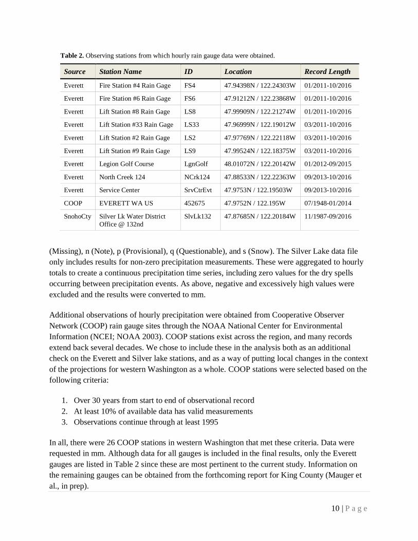
(Missing), n (Note), p (Provisional), q (Questionable), and s (Snow). The Silver Lake data file

only includes results for non-zero precipitation measurements. These were aggregated to hourly

totals to create a continuous precipitation time series, including zero values for the dry spells

occurring between precipitation events. As above, negative and excessively high values were

excluded and the results were converted to mm.

Additional observations of hourly precipitation were obtained from Cooperative Observer

Network (COOP) rain gauge sites through the NOAA National Center for Environmental

Information (NCEI; NOAA 2003). COOP stations exist across the region, and many records

extend back several decades. We chose to include these in the analysis both as an additional

check on the Everett and Silver lake stations, and as a way of putting local changes in the context

of the projections for western Washington as a whole. COOP stations were selected based on the

following criteria:

1. Over 30 years from start to end of observational record

2. At least 10% of available data has valid measurements

3. Observations continue through at least 1995

In all, there were 26 COOP stations in western Washington that met these criteria. Data were

requested in mm. Although data for all gauges is included in the final results, only the Everett

gauges are listed in Table 2 since these are most pertinent to the current study. Information on

the remaining gauges can be obtained from the forthcoming report for King County (Mauger et

al., in prep).

Table 2. Observing stations from which hourly rain gauge data were obtained.

Source Station Name ID Location Record Length

Everett Fire Station #4 Rain Gage FS4 47.94398N / 122.24303W 01/2011-10/2016

Everett Fire Station #6 Rain Gage FS6 47.91212N / 122.23868W 01/2011-10/2016

Everett Lift Station #8 Rain Gage LS8 47.99909N / 122.21274W 01/2011-10/2016

Everett Lift Station #33 Rain Gage LS33 47.96999N / 122.19012W 03/2011-10/2016

Everett Lift Station #2 Rain Gage LS2 47.97769N / 122.22118W 03/2011-10/2016

Everett Lift Station #9 Rain Gage LS9 47.99524N / 122.18375W 03/2011-10/2016

Everett Legion Golf Course LgnGolf 48.01072N / 122.20142W 01/2012-09/2015

Everett North Creek 124 NCrk124 47.88533N / 122.22363W 09/2013-10/2016

Everett Service Center SrvCtrEvt 47.9753N / 122.19503W 09/2013-10/2016

COOP EVERETT WA US 452675 47.9752N / 122.195W 07/1948-01/2014

SnohoCty Silver Lk Water District

Office @ 132nd

SlvLk132 47.87685N / 122.20184W 11/1987-09/2016

11 | P a g e

The COOP data include two quality control flags: a “Measurement” and a “Data Quality” flag.

Observations were treated as missing values if any of these flags were present, with one

exception: data flagged as Trace precip (“T”) were set to zero (valid data, no precipitation).

Additional inspection of the COOP data revealed periods when precipitation was zero for long

stretches, extending beyond one month without precipitation, yet there were no flags to indicate

missing data. Data checks with other gauge networks, showed that dry spells of this length do not

happen in the region, even in the relatively drier eastern half of the state. As a result, two

additional quality control checks were added to the data: (1) data were set to missing when all-

zeros stretches extended to more than 60 consecutive days, and (2) COOP stations were only

included if 95% of available data was present for at least 30 water years (Oct-Sep). By applying

these additional criteria, we were able to remove the vast majority of questionable data.

Finally, two data considerations are worth noting. First, the Everett rain gauge records are quite

short, limiting the accuracy of the precipitation statistics that can be obtained. This is evident in

the results that are presented below. As a result, we recommend a focus on the results for the

Silver Lake, with the Everett COOP station in Everett serving as a check on those results. Second,

although we have made every attempt to comprehensively remove errors in the observations,

some anomalous values may remain, and these errors could affect the bias correction of the

model projections. For this reason, we have included extensive information on model biases,

both before and after bias correction, in the products outlined below. In addition, we recommend

using the percent changes as opposed to the absolute model projections in stormwater planning

and design.

12 | P a g e

6 Post-Processing

6.1 WRF data extraction

The WRF outputs are on a curvilinear 12-km grid. The model outputs separate precipitation

estimates based on whether it is simulated as a result of the convective parameterization

occurring at the sub-grid scale or as part of a large-scale process that is resolved by the model.

As is typical, precipitation was calculated as the sum of these two quantities.

Hourly data were extracted for the nearest grid point to each rain gauge station (nearest-neighbor

interpolation). These constitute the “raw” WRF data for each station dataset. Since the WRF

resolution is coarse compared to the spacing of the rain gauge stations, many stations have

identical raw WRF data.

Although WRF projections represent a substantial improvement over previous downscaled

precipitation estimates, the simulations do contain biases. Many applications require estimates of

absolute precipitation totals, especially those that involve continuous simulation of stormwater or

other system performance. In these cases, it is not always practical to apply a simple percent

change to observed historical precipitation intensities, such as those typically obtained from an

intensity-duration-frequency relationship. As a result, the raw WRF data were additionally bias-

corrected to match the observations at each rain gauge site.

6.2 Bias Correction

For each station location, the raw WRF hourly precipitation was bias corrected to the historical

hourly station data. Observed data were quality controlled as described in Section 5.3, and the

full period of record was used for each station.

Although bias correction is a key tool used in many applications, recent work has shown that it

can introduce artifacts in the case of climate change, especially when considering changes in

extremes (Mauger et al. 2016). In principle one could design a bias correction approach that

controls for the sensitivity of climate change. However, such an approach has never been

developed and in fact may not be feasible given the limits of observational data and the fact that

a statistical approach may not be able to capture complex changes in the processes and responses

governing local weather and climate. As a result, our focus in this study is to develop a bias

correction approach that strikes a compromise between improved accuracy in the historical

simulations while preserving the projected changes from the raw WRF data.

13 | P a g e

The simplest approach to bias correction is to simply scale the model precipitation so that the

model average matches the average in the observations. This is sometimes referred to as the

“Delta” method. An advantage of this approach is that it has no effect on the projected changes.

However, inspection of the raw model results shows that WRF tends to overestimate the

intensity of light rain and underestimate the intensity of heavy rain events. This suggests that a

simple Delta approach will not be adequate, since the bias is not the same for all precipitation

intensities. Recent approaches to bias correction have typically emphasized a quantile-mapping

approach, in which the probability distribution from the model is adjusted to match the observed

probability distribution in precipitation (e.g., Abatzoglou and Brown 2012). While this method is

quite effective at reducing the historical biases, including those for the extremes, our tests show

that it can introduce substantial biases in the projected changes (Figure 3; these results confirm

previous findings by Mauger et al. 2016), particularly for extreme events. These discrepancies

exist because the correction for one quantile in the historical data can be quite different than the

correction for the same quantile in the future due to the projected changes in precipitation

intensity and the limited accuracy in estimating the highest quantiles of the distribution. This

cannot be readily corrected by removing the long-term trends because the trends are also

different for different quantiles. This problem is complicated by the fact that quantile estimates

from a finite sample will always have limited accuracy in the extreme tails of the distribution.

For this study, we developed a compromise approach, called the “Percentile-Delta” method,

which combines the intensity-based scaling of the quantile mapping approach with the stability

Figure 3. Comparison of bias correction approaches for the Everett COOP rain gauge station. The figure

compares the performance of two bias-correction approaches: the recently-developed quantile mapping approach

and the “Percentile-Delta” method used in this study. Both plots show the statistics for the 2-, 10-, 25-, and 100-

year extremes in hourly water year precipitation (50%, 10%, 4%, and 1% annual chance of exceedance,

respectively). The left-hand plot compares the bias corrected model results to both the raw model results and the

observations. Both bias-correction approaches lead to an improvement over the raw results. The right-hand plot

compares the percent change in precipitation intensity at each return interval for 2070-2099 (2080s), relative to

1970-1999 (1980s). In this plot we see that the Percentile-Delta approach closely matches the raw projection,

while the quantile-mapping approach diverges substantially from the change projected by the model.

14 | P a g e

of the Delta method. In this approach, the historical and future WRF data are adjusted by

correcting mean biases in precipitation in each quantile range (i.e. 0-1, 1-2, … 99-100). First, all

model precipitation values below 0.001 inch (0.025 mm) were set to zero. This is a common

approach since models simulate a continuous distribution of precipitation yet measurements

cannot resolve quantities less than about 0.01 inch (0.25 mm). Next, adjustments were computed

in each percentile of precipitation as the ratio of the average from the historical WRF data (1970-

2005) to that from the full observational record. The result is a different set of “deltas” for each

percentile. A separate set of ratios was calculated for the future WRF simulation (2006-2099).

These ratios were then applied to all values in each percentile of the historical and future WRF

data, respectively. Note that this means that the adjustment applied to a specific precipitation

amount (e.g., 5 mm/hr) may be different for the historical and future simulations. This is

equivalent to assuming that the mechanisms governing precipitation are a function of the

quantile in hourly precipitation as opposed to the total amount. Recent research supports this

assumption (e.g., Warner et al. 2015), indicating that changes in storm thermodynamics (water

vapor concentration) and not dynamics (e.g., strength or direction of winds) is the primary driver

of increases in precipitation intensity.

The Percentile-Delta method was chosen over other methods after extensive testing and

evaluation of alternative approaches, applied to both daily and hourly precipitation. The results

from these experiments revealed that biases in daily precipitation could be very different than

projected changes in hourly precipitation, so that direct bias correction of hourly data was

preferable to the bias correction of daily data and subsequent scaling to an hourly time step. In

addition, projected changes in return intervals of hourly precipitation were best preserved when

performing the Percentile-Delta method versus other methods including quantile-mapping,

quantile-mapping with smoothed probability distributions, and applying just two Delta scaling:

one for precipitation below the 99th percentile, and another for all precipitation above it. For all

approaches, including the Percentile-Delta method, the degree of historical agreement with

observations and consistency with raw model projections differed greatly by station location (e.g.,

wet or dry locations) and by the length of the observational record (e.g., shorter records

sometimes showed worse results).

6.3 Summary Statistics

Precipitation totals and extreme statistics were calculated for four 30-year time periods: 1970-

1999 (“1980s”), 2020-2049 (“2030s”), 2040-2069 (“2050s”), and 2070-2099 (“2080s”).

Although longer time periods might be desired to estimate extreme statistics, 30 years was

deemed an appropriate compromise between longer periods, which may conflate long-term

changes in flood risk with increased sampling of the extremes, and shorter time periods, which

can limit the reliability of extremes estimates.

15 | P a g e

Since limited sample size can lead to errors in these either the multi-year averages or extremes

statistics, these were only calculated if the following conditions were met:

1. A minimum of 90% valid observations (< 10% missing values) to estimate the maximum

or total for the water year or month in question.

2. A minimum of 5 years of valid observations to compute the long-term average (e.g., of

total water year precipitation).

3. A minimum 10 years of valid observations to compute the 2-year extreme, and 25 years

of valid data to compute the 5-, 10-, 25-, 50-, and 100-year extremes.

These conditions were chosen as a compromise between ensuring that the estimates are robust

and the desire to include as many observational records as feasible in the analysis. Caution is

advised regarding the results for the 50- and 100-year events, for which a 25-year record will

likely be too short to produce robust estimates.

6.4 Extreme Value Analysis

For many applications, the key metric is the change in the intensity of specific design storms.

The raw and bias-corrected data were both processed to estimate exceedance values for both

monthly and water year (Oct-Sep) extremes. These calculations followed the standard block-

maximum approach, fitted to an extreme distribution using l-moments (Hosking and Wallis

2005).

To calculate extreme statistics, the Extreme Value type 1 distribution described by Gumbel

(EV1), the Log-Pearson type 3 (LP3), and the generalized Extreme Value (GEV) distribution

with L-moments are commonly used. In this study we apply the GEV distribution with L-

moments to estimate extreme precipitation statistics – following the methodology described in

Salathé et al. 2014 and Tohver et al. 2014 – based on findings that indicate it is superior to the

LP3 distribution (Rahman et al. 1999 & 2015, Vogal et al. 1993, Nick et al. 2011).

Calculations were applied to multiple precipitation durations ranging from 1 hour to 15 days, and

the precipitation intensities estimated for following recurrence intervals: 2-, 5-, 10-, 25-, 50-, and

100-year events (50%, 20%, 10%, 4%, 2%, and 1% annual chance of exceedance, respectively).

16 | P a g e

7 Results

All results from this study are available online and can be accessed via the link below. A Google

Map has also been created for identifying stations to facilitate navigation of the results directory.

In addition, we have produced a series of summaries and visualizations that can be used to view

the results.

• Direct link to results:

http://cses.washington.edu/picea/mauger/2017_12_KingCounty_Stormwater/DATA/pub

• Google Map for locating stations: https://goo.gl/6rDsRH

• Interactive visualizations for viewing results: https://doi.org/10.7915/CIG4QJ78R

• Spreadsheet summarizing the projected changes for all durations for the 2030s, 2050s,

and 2080s.

The interactive visualizations include three separate viewers to allow users to view model biases

relative to observations, view the percent changes for multiple recurrence intervals, and evaluate

each of these for different precipitation durations.

ResultsModel & Scenario

Data Type

Rain Gauge Sites

Pub Folder

pub/

gauge name

OBS

rawWRF

ACCESS / RCP 4.5

hourly time series

hourly, precip>0

water year maxima

monthly maxima

statistics

GFDL / RCP 8.5

bcWRF...

...

gauge name

Figure 4. Data structure for study results.

17 | P a g e

7.1 Data Structure

The organization of the online repository is shown in Figure 4. All files are comma-delimited

(.csv), and all values are in millimeters (mm). There are five types of output files, with the

following naming conventions:

1. Hourly time series files. Time series including the full record of observational, raw, and

bias-corrected hourly precipitation. For the WRF files these are split into historical

(1970-2005) and future (2006-2099) files in order to accommodate the maximum number

of rows allowed in Excel. Since the full 130-year hourly time series creates files that are

too long for Excel, additional files are provided that separate the historical and future

model simulations.

File naming: <Network>_<ID>_<lat>_<long>_<raw/bcWRF>_<model>_<scenario>.csv

<Network>_<ID>_<lat>_<long>_<raw/bcWRF>_<model>_<scenario>.1970-2005.csv

<Network>_<ID>_<lat>_<long>_<raw/bcWRF>_<model>_<scenario>.2006-2099.csv

2. Time series of non-zero precipitation. These are the same as the previous files, except

that all zero values of precipitation are removed. For the WRF files, any precipitation

value less than 0.001 inch (0.025 mm) were set to zero.

File naming: <Network>_<ID>_<lat>_<long>_<raw/bcWRF>_<model>_<scenario>.non-zero.csv

3. Water year maxima. Maximum precipitation for each water year (Oct-Sep), for 11

different durations (1-, 2-, 3-, 6-, 12-, 24-, 48-, 72-, 120-, 240-, and 360-hour

precipitation). These are used as the basis for the extremes calculations described in

Section 6.4.

File naming: <Network>_<ID>_<lat>_<long>_<raw/bcWRF>_<model>_<scenario>.WYmax.csv

4. Monthly maxima. Same as #3 except showing the maximum for each month.

File naming: <Network>_<ID>_<lat>_<long>_<raw/bcWRF>_<model>_<scenario>.MOmax.csv

5. Extreme Statistics. Extreme statistics, for historical and future time periods, for all return

intervals and precipitation durations. Two files are included: one listing the absolute

totals for each statistic, and another listing the percent change for three future time

periods.

File naming: <Network>_<ID>_<lat>_<long>_<raw/bcWRF>_<model>_<scenario>.stats-abs_vals.csv

<Network>_<ID>_<lat>_<long>_<raw/bcWRF>_<model>_<scenario>.stats-pct_chg.csv

18 | P a g e

The observational data file naming is slightly different, since these are not based on a specific

model. The file names for these are identical to those listed above, with the following exceptions:

1) The observational data file includes the latitude and longitude of the rain gauge, whereas

the WRF files list the position of the nearest model grid point.

2) The WRF-specific suffix ‘<raw/bcWRF>_<model>_<scenario>’ is removed, since it does

not apply to the observations.

3) There is no percent change file for the statistics, since these files list future changes and

are therefore not applicable to the observational record.

7.2 Summary: Projected Changes in 1-hour Precipitation Extremes

Projected changes in the 1-hour precipitation statistics are summarized in Table 3, for the 2080s

(2070-2099) relative to 1970-1999. Projections for other precipitation durations and for the

2030s (2020-2049) and 2050s (2040-2069) are included in a spreadsheet accompanying this

report. Before summarizing the results, a number of points should be made about the

interpretation of these projections:

• Projected changes will always be governed by a combination of random variability and

long-term trends due to climate change. This is particularly true for changes in extremes:

Since by definition these events are rare, it is difficult to accurately assess how rapidly

they will change. Although even the 2080s projections can be significantly influenced by

natural variability, we recommend focusing on these late century projections since this is

when the projected changes will be largest relative to natural variability.

• The 50- and 100-year estimates are likely more prone to noise since they are estimated

from a 30-year record (e.g., 1970-1999, 2070-2099).

• Projected changes differ substantially for different precipitation durations. In general,

changes appear to be largest for 1-hour precipitation and smallest for the longest

durations. This is consistent with previous research projecting a change in atmospheric

river events yet very little change in seasonal precipitation.

• The two scenarios were selected based on an interpretation of the global model

projections, which may not always be a good predictor of the results of the corresponding

WRF simulations. Indeed, it is clear from Table 3 that the two scenarios do not even

consistently correspond to their “Low” and “High” titles.

• Similarly, the two scenarios are unlikely to bracket the full range of potential future

outcomes. Instead, these should be viewed as two equally-likely future projections which

should be accounted for in planning and design. Future work can provide additional WRF

simulations, from which we could obtain a more robust estimate of the mean and range

among projections.

19 | P a g e

• The WRF model used in this study has a spatial resolution of 12 km. This is not enough

to explicitly resolve convective precipitation, such as thunderstorms. Although these are

represented statistically by the model, researchers generally consider that a finer

resolution is needed to accurately capture convective events. This means that the current

projections should be viewed primarily as an estimate of the change in the intensity of

large-scale heavy precipitation events such as atmospheric rivers.

• In this study, extremes were estimated by fitting a GEV distribution with l-moments

(Section 6.4). This approach will result in different estimates than the standard (e.g.,

Bulletin 17B, 1982) methods that are prescribed in certain applications. In most cases,

these differences should be minor. However, we recommend repeating the calculations

using the prescribed methodology to ensure consistent results and interpretation.

Focusing on the 25-year event (4% annual chance of exceedance), results show a +1 to +28%

increase in the water year extreme. Seasonally, the simulations show the largest increase for

Table 3. Projected changes (%) in 1-hour precipitation statistics for the WRF grid point closest to the

Silver Lake rain gauge, for the 2080s (2070-2099) relative to 1970-1999. Columns show the changes for

both WRF scenarios for the full water year (Oct-Sep), as well as for winter (Dec-Feb), spring (Mar-May),

summer (Jun-Aug), and fall (Sep-Dec). Rows show the projected change in the total accumulation for

each time period as well as for the 2-, 5-, 10-, 25-, 50-, and 100-year events.

Water Year Dec-Feb Mar-May Jun-Aug Sep-Dec

AC

CE

SS

1.0

- R

CP

4.5

(L

ow

)

GF

DL

CM

3 -

RC

P 8

.5 (

Hig

h)

AC

CE

SS

1.0

- R

CP

4.5

(L

ow

)

GF

DL

CM

3 -

RC

P 8

.5 (

Hig

h)

AC

CE

SS

1.0

- R

CP

4.5

(L

ow

)

GF

DL

CM

3 -

RC

P 8

.5 (

Hig

h)

AC

CE

SS

1.0

- R

CP

4.5

(L

ow

)

GF

DL

CM

3 -

RC

P 8

.5 (

Hig

h)

AC

CE

SS

1.0

- R

CP

4.5

(L

ow

)

GF

DL

CM

3 -

RC

P 8

.5 (

Hig

h)

Total -1 4 -3 17 -1 19 -56 -39 14 4

2-yr 26 26 21 20 22 21 -58 10 17 40

5-yr 24 40 31 36 29 20 -54 18 16 44

10-yr 25 50 37 56 34 16 -53 18 15 48

25-yr 28 63 46 92 40 9 -52 15 14 56

50-yr 31 73 53 130 44 2 -51 12 14 62

100-yr 34 83 59 180 48 -5 -51 8 13 70

20 | P a g e

winter and a consistent and a substantial decrease in summer, with more modest increases for

spring and fall. Although projected changes differ substantially among return intervals (2-yr

event, 5-yr event, etc.), there is some consistency, especially in the projections for summer. As

noted above, the simulations may not adequately capture changes in thunderstorm intensity –

since this is an important source of heavy rainfall in summer, the current projections may not

adequately represent expected changes in summer extremes.

21 | P a g e

8 References

Abatzoglou, J. T., & Brown, T. J. (2012). A comparison of statistical downscaling methods

suited for wildfire applications. International Journal of Climatology, 32(5), 772-780.

http://onlinelibrary.wiley.com/doi/10.1002/joc.2312/full

Bi D, Dix M, Marsland S, O’Farrell S, Rashid H, Uotila P, et al. The Access Coupled Model:

Description, Control Climate and Evaluation. Australian Meteorological and

Oceanographic Journal. 2013; 63:41-64. http://dx.doi.org/10.22499/2.6301.004

Griffies, S. M., Winton, M., Donner, L. J., Horowitz, L. W., Downes, S. M., Farneti, R., ... &

Palter, J. B. (2011). The GFDL CM3 coupled climate model: characteristics of the ocean

and sea ice simulations. Journal of Climate, 24(13), 3520-3544.

https://doi.org/10.1175/2011JCLI3964.1

Hosking, J. R. M., & Wallis, J. R. (2005). Regional frequency analysis: an approach based on L-

moments. Cambridge University Press.

(Bulletin 17-B) U.S. Interagency Advisory Committee on Water Data, 1982, Guidelines for

determining flood flow frequency, Bulletin 17-B of the Hydrology Subcommittee: Reston,

Virginia, U.S. Geological Survey, Office of Water Data Coordination, [183 p.].

[Available from National Technical Information Service, Springfield VA 22161 as report

no. PB 86 157 278 or from FEMA at http://www.fema.gov/mit/tsd/dl_flow.htm

Mauger, G.S., S.-Y. Lee, C. Bandaragoda, Y. Serra, J.S. Won, 2016. Refined Estimates of

Climate Change Affected Hydrology in the Chehalis basin. Report prepared for Anchor

QEA, LLC. Climate Impacts Group, University of Washington, Seattle.

https://doi.org/10.7915/CIG53F4MH

Nick, M., Das, S. and Simonovic, S.P. 2011. The Comparison of GEV, Log-Pearson Type 3 and

Gumbel Distributions in the Upper Thames River Watershed under Global Climate

Models, the University of Western Ontario Department of Civil and Environmental

Engineering, Report No:077. https://ir.lib.uwo.ca/wrrr/40/

(NOAA) U.S. Department of Commerce, National Oceanic and Atmospheric Administration,

National Centers for Environmental Information (NCEI). (2003). DATA

DOCUMENTATION FOR DATA SET 3240 (DSI-3240); Hourly Precipitation Data.

https://www.ncdc.noaa.gov/IPS/hpd/hpd.html

22 | P a g e

Rahman, A., Weinmann, P.E. and Mein, R.G. (1999). At-site flood frequency analysis: LP3-

product moment, GEV-L moment and GEV-LH moment procedures compared. In:

Proceeding Hydrology and Water Resource Symposium, Brisbane, 6–8 July, 2, 715–720.

Rahman, A., Karin, F, and Rahman, A. 2015. Sampling Variability in Flood Frequency Analysis:

How Important is it? 21st International Congress on Modelling and Simulation, Gold

Coast, Australia, Nov 29-Dec 4, 2015, 2200-2206.

Salathé Jr., Eric P., Alan F. Hamlet, Clifford F. Mass, Se-Yeun Lee, Matt Stumbaugh, and

Richard Steed, 2014: Estimates of Twenty-First-Century Flood Risk in the Pacific

Northwest Based on Regional Climate Model Simulations. J. Hydrometeor, 15, 1881–

1899. doi: http://dx.doi.org/10.1175/JHM-D-13-0137.1

Tohver, I. M., Hamlet, A. F., & Lee, S. Y. (2014). Impacts of 21st‐Century Climate Change on

Hydrologic Extremes in the Pacific Northwest Region of North America. JAWRA

Journal of the American Water Resources Association, 50(6), 1461-1476.

https://doi.org/10.1111/jawr.12199

Trenberth, K. E. (2011). Changes in precipitation with climate change. Climate Research, 47(1-

2), 123-138. http://dx.doi.org/10.3354/cr00953

Van Vuuren, D., J. Edmonds, M. Kainuma, K. Riahi, A. Thomson, K. Hibbard, G. Hurtt, T.

Kram, V. Krey, J. Lamarque, T. Masui, M. Meinshausen, N. Nakicenovic, S. Smith, S.

Rose, 2011: The representative concentration pathways: an overview. Climatic Change,

109: 5-31. http://dx.doi.org/10.1007/s10584-011-0148-z

Vogel, R.M., McMahon, T.A. and Chiew, F.H.S. (1993). Flood flow frequency model selection

in Australia, Journal Hydrology, 146, 421-449. https://doi.org/10.1016/0022-

1694(93)90288-K

Warner, M. D., Mass, C. F., & Salathé Jr, E. P. (2015). Changes in winter atmospheric rivers

along the North American west coast in CMIP5 climate models. Journal of

Hydrometeorology, 16(1), 118-128. https://doi.org/10.1175/JHM-D-14-0080.1

23 | P a g e

9 Appendix: Email description of data modifications to Silver Lake Gauge

James C. (Jim) Peterson

PE, PMP

HDR Engineering, Inc.

Professional Associate |Senior Engineer

500 108th Ave NE, Suite 1200 | Bellevue, WA 98004

425.450.6308 (direct) | c: 425.765.3291

Jim.Peterson@hdrinc.com | hdrinc.com

Follow Us – Facebook | Twitter | YouTube

From: Mel Schaefer [mailto:mgschaefer@mgsengr.com] Sent: Friday, November 04, 2011 2:52 PM To: Peterson, Jim; 'Drangsholt, Steven' Subject: Silver Lake Time­Series

Jim and Steve:

Here are the two 5­minute precipitation time­series for the Silver Lake Gage (second e­mail to followdue to file size). The files are condensed, that is zero precipitation values have been removed. The“raw” precipitation time­series is essentially the data as recorded at the Silver Lake gage. The“Interim” precipitation time­series is the rescaled version of the Silver Lake time­series as described inthe Nov 3, 2011 memorandum. The interim time­series should be adequate for rainfall­runoffmodeling and making the first rough cut where a given portion of the sewer system can becharacterized as being clearly adequate, marginal, or clearly inadequate based on proposed servicelevels.

CHANGES TO BOTH TIME­SERIES FILES

The missing period from Oct 1, 1987 through Nov 20, 1987 at the start of the 1988 water­year hasbeen filled using data from the Haller Lake Gage (SPU). This provides a start­up period for rainfall­runoff modeling for the 1988 water year. There is nothing noteworthy in this period in the way ofstorms, so it won’t cause any distortion in the assessment of system service levels.

Data with quality flags of “eh” (estimated hourly amount) were disaggregated to eliminate thepossibility of a large 5­minute spike of runoff. There were a few hourly values exceeding 1­inchoriginally allocated to a 5­minute period. For isolated small hourly amounts, less than 0.04­inch, theamount was allowed to be assigned to a 5­minute interval. Moderate amounts were randomlysmeared over the hour period and larger “eh” hourly precipitation amounts were disaggregated usinga temporal pattern from the Haller Lake gage.

RAW TIME­SERIES FILES

The “Raw” file is essentially the observed record at Silver Lake formatted at a 5­minute time­step, withthe adjustments described above.

INTERIM TIME­SERIES

The “Interim” time­series has been rescaled according to the procedures described in the Nov 3, 2011memorandum. The time­series has precipitation­frequency characteristics in the durations from 5­minutes through 6­hours that reasonably replicate the characteristics expected for the EverettMetropolitan area. Precipitation at the 24­hour duration is about 10% above what would be expectedin the Everett area. Sewer systems that are sensitive to runoff volume rather than peak flow mayshow less capacity for larger storms than is actually the case. The 10% greater precipitationamounts in the long­duration storms (24­hours and greater) shouldn’t dramatically alter the decisionabout placement in the 3 performance bins. The time­series does contain the Dec 2007 long­duration storm which is on the order of a 100­year event and will likely cause problems forcomponents of the sewer system that are sensitive to runoff volume.

PRECIPITATION TIME­SERIES FOR FINAL ANAYSES

I will be working on development of 5­minute precipitation time­series using statistical scalingprocedures and the Silver Lake data. The resultant precipitation time­series will replicate theprecipitation­frequency characteristics expected in the Everett area for durations from 5­minutesthrough 72­hours. This time­series will replace the “Interim” time­series as soon as it is completed.

If you have any questions, just give me a call or send an e­mail.

­­Mel

Mel Schaefer

MGS Engineering Consultants, Inc.

7326 Boston Harbor Road NE

Olympia, WA 98506

phone: (360) 570­3450

fax: (360) 570­3451

­­­­­­­­­­ Message transféré ­­­­­­­­­­ From: "Peterson, Jim" <Jim.Peterson@hdrinc.com> To: Souheil Nasr <SNasr@everettwa.gov> Cc: "Bergstrom, Eric" <Eric.Bergstrom@hdrinc.com>