NEW QUADRATURE FORMULAS FROM …people.maths.ox.ac.uk/trefethen/publication/PDF/2008_128.pdfNEW QUADRATURE FORMULAS FROM CONFORMAL MAPS AND ... ANAL. c 2008 Society for Industrial

Copyright © by SIAM. Unauthorized reproduction of this article is prohibited.

SIAM J. NUMER. ANAL. c© 2008 Society for Industrial and Applied MathematicsVol. 46, No. 2, pp. 930–948

NEW QUADRATURE FORMULAS FROM CONFORMAL MAPS∗

NICHOLAS HALE† AND LLOYD N. TREFETHEN†

Abstract. Gauss and Clenshaw–Curtis quadrature, like Legendre and Chebyshev spectral meth-ods, make use of grids strongly clustered at boundaries. From the viewpoint of polynomial approx-imation this seems necessary and indeed in certain respects optimal. Nevertheless such methodsmay “waste” a factor of π/2 with respect to each space dimension. We propose new nonpolynomialquadrature methods that avoid this effect by conformally mapping the usual ellipse of convergenceto an infinite strip or another approximately straight-sided domain. The new methods are com-pared with related ideas of Bakhvalov, Kosloff and Tal-Ezer, Rokhlin and Alpert, and others. Anadvantage of the conformal mapping approach is that it leads to theorems guaranteeing geometricrates of convergence for analytic integrands. For example, one of the formulas presented is proved toconverge 50% faster than Gauss quadrature for functions analytic in an ε-neighborhood of [−1, 1].

Key words. Gauss quadrature, Clenshaw–Curtis quadrature, spectral methods, conformalmapping

AMS subject classifications. 65D32, 30C20

DOI. 10.1137/07068607X

1. Introduction. The Gauss and Clenshaw–Curtis quadrature formulas, as wellas other related numerical methods for integration of nonperiodic functions or spectralsolution of nonperiodic ODEs or PDEs, all cluster the grid points near the boundaries.Indeed, for any convergent numerical method derived from polynomial interpolationin the grid points, the clustering will be asymptotically the same: on [−1, 1], n pointswill be distributed with density ∼ n/(π

√1 − x2 ) as n → ∞ [36, Thm. 12.7].

It is well known that this clustering may cause problems. The high density ofpoints near the boundaries may necessitate very small time steps in an explicit time-stepping spectral method or make the matrices involved in implicit time-steppingterribly ill conditioned [12, 49]. At the same time the low density of points in themiddle of the domain may force one to use more points than “ought” to be needed toresolve the solution. Compared with equally spaced grids, these clustered grids haveπ/2 times coarser spacing in the middle, implying that, for many calculations, n mustbe about π/2 times larger than one might expect. In a three-dimensional calculation,a discretization may need (π/2)3 ≈ 4 times as many grid points as one would like.Such a factor may have a large impact on the cost of linear algebra operations.

In this article we focus on this π/2 problem and mainly on quadrature, not spec-tral, methods. The problem arises in purest form if we consider the integral from −1to 1 of a function f analytic in a narrow strip about the real axis. If f is periodic,we can use the trapezoid rule and get geometric convergence, i.e., convergence at arate e−Cn for some C > 0. If f is not periodic, the trapezoid rule loses its speed, butGauss quadrature still converges geometrically. However, the constant C is π/2 timessmaller, and thus the convergence rate is π/2 times slower.

Various authors have proposed methods for countering this effect. We shall sug-gest a new approach based on conformal mapping, which leads to formulas that

∗Received by the editors March 22, 2007; accepted for publication (in revised form) August 31,2007; published electronically March 5, 2008.

http://www.siam.org/journals/sinum/46-2/68607.html†Oxford University Computing Laboratory, Wolfson Bldg., Parks Rd., Oxford OX1 3QD, UK

([email protected], [email protected]).

930


NEW QUADRATURE FORMULAS 931

converge more quickly than Gauss quadrature for many integrands. The practicalperformance of our methods is not much different from that of other methods in theliterature, such as those of Alpert [3] and Kosloff and Tal-Ezer [33] (see section 5).Nevertheless, the conformal mapping idea has advantages. First, it is conceptuallyclear, simple, and flexible, explaining in a precise way the nature of the π/2 effectand exactly what improvements may be possible for integrands analytic in specifieddomains. Second, it leads immediately to theorems on geometric convergence ratesfor analytic integrands. In the existing literature of related methods, it is hard tofind such theorems. An additional advantage, which we shall not discuss further,is that the conformal mapping approach connects these simple quadrature problemsto more complicated problems where conformal maps have also proved useful, suchas the double exponential quadrature formula and Tee’s adaptive rational spectralmethods [22, 38, 43, 44, 46, 47, 48].

An outline of the article is as follows. In section 2 we present the conformal trans-plantation idea. We apply it in section 3 to the particular case of a map to an infinitestrip and in section 4 to a simpler variant that may be equally useful in practice. Re-lated work is surveyed in section 5, and theorems about geometric convergence ratesare presented in section 6. The Clenshaw–Curtis variant of our formulas is consideredin section 7, and we close in section 8 with a summary discussion. The appendixincludes a 14-line FFT-based MATLAB code that runs in less than a second for n ashigh as 105 yet usually delivers more accurate integrals than the Gauss rule for eachvalue of n.

2. Transplanted quadrature formulas. Let f be an analytic function on[−1, 1] whose integral

I = I(f) =

∫ 1

−1

f(x)dx(2.1)

we seek to calculate. A general interval [a, b] can be handled by a linear change ofvariables. All of the methods we shall consider approximate I by sums

In = In(f) =

n∑k=1

wkf(xk)(2.2)

defined by nodes {xk} and weights {wk}. Polynomial methods of this kind are basedon the following principle: given nodes {xk}, the weights {wk} are chosen so that Inis equal to the integral of the unique degree n − 1 polynomial interpolant throughthe data points. In particular, Newton–Cotes quadrature is obtained from equallyspaced nodes, Gauss quadrature from the roots of the Legendre polynomial Pn, andClenshaw–Curtis quadrature from the Chebyshev points xk = cos((k − 1)π/(n− 1)).Any polynomial method that converges as n → ∞ for all analytic f must have itsnodes distributed asymptotically with density ∼ n/(π

√1 − x2 ) as n → ∞. The Gauss

and Clenshaw–Curtis formulas have this property and converge for any continuous f .The Newton–Cotes formulas do not and diverge in general even if f is analytic [5, 36,41].

The standard theorems about convergence of polynomial methods for analyticfunctions assume that the integrand is analytic in an elliptical region. For any ρ > 1,let us define Eρ to be the open set in the complex plane bounded by the ellipse withfoci ±1 with semiminor and semimajor axis lengths summing to ρ. This ellipse canalso be described as the image of the circle of radius ρ about the origin under the


932 NICHOLAS HALE AND LLOYD N. TREFETHEN

−1 1

Eρ

g

−1 1

Ωρ

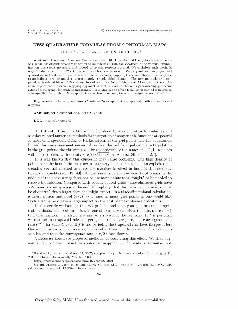
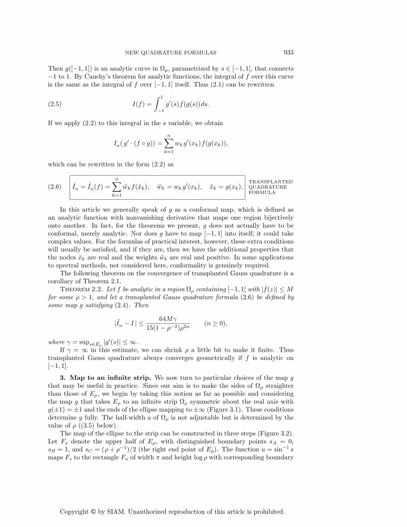
Fig. 2.1. A transplanted quadrature formula (2.6) is defined by an analytic function g thatmaps the elliptical region Eρ into a region Ωρ containing [−1, 1]. In this illustration the map isg(s) = 0.5s + 0.2s3 + 0.3s5 with ρ = 1.4. The dots show Gauss points xk ∈ Eρ for n = 16 and theirimages xk ∈ Ωρ.

map w = (z + z−1)/2. The general idea of the following convergence theorem goesback to Bernstein in 1919 [8], but such results do not appear in many textbooksor monographs, and there is not much uniformity in the constants that one findson the right-hand side [25, p. 114]. The particular result presented here is due toRabinowitz [42, eq. (18)]; see also [11, Thm. 90] and [50, Thm. 4.5].

Theorem 2.1. If f is analytic in Eρ, with |f(z)| ≤ M for some ρ > 1, thenGauss quadrature converges geometrically with the bound

|In − I | ≤ 64M

15(1 − ρ−2)ρ2n(n ≥ 0).(2.3)

When we don’t care about constants, we may simply note that Theorem 2.1ensures geometric convergence at the rate O(ρ−2n) as n → ∞.

To experts in approximation theory, the assumption of analyticity in an ellipticalregion is so familiar as to seem almost beyond question. Nevertheless, the appearanceof ellipses in this analysis is driven not by the quadrature formula (2.2) per se but bythe decision to derive weights from polynomial interpolation. If we do not insist onpolynomials, ellipses cease to have any special status.

We have already observed from the uneven distribution of Gauss and Clenshaw–Curtis nodes that there may be a reason to move beyond polynomials. Here is anotherargument based on the shape of Eρ. From an applications point of view, the assump-tion that f is analytic in Eρ is unbalanced, for it permits f to be “less analytic” nearthe ends of the interval, where the ellipse is narrow, than in the middle, where it iswide. Specifically, the Taylor series of f at a point x ≈ ±1 is allowed to have morerapidly increasing coefficients than are permitted at a point x ≈ 0. This nonuniformanalyticity condition leads to Theorem 2.1 and related results for other polynomialquadrature formulas, but it has no intrinsic justification. Further consequences of thesame nonuniformity reverberate throughout the field of polynomial approximationtheory—for example, in the book by Ditzian and Totik [17]. Of course, there are ap-plications where the functions of interest do have less smoothness near the boundarythan in the interior, such as fluid mechanics problems with boundary layers. Evenhere, however, there is no reason to expect that an ellipse should be exactly the rightregion to consider. Weak boundary layers might benefit from less grid clustering atboundaries and strong ones from even more.

Our plan is to derive new quadrature formulas (2.2) for [−1, 1] by conformallymapping Eρ to a region Ωρ that has straighter sides. We describe the procedure firstin general terms; see Figure 2.1.

Let Ωρ be an open set in C containing [−1, 1] inside of which the function f isanalytic. Let g be an analytic function in Eρ satisfying

g(Eρ) ⊆ Ωρ, g(−1) = −1, g(1) = 1.(2.4)



Then g([−1, 1]) is an analytic curve in Ωρ, parametrized by s ∈ [−1, 1], that connects−1 to 1. By Cauchy’s theorem for analytic functions, the integral of f over this curveis the same as the integral of f over [−1, 1] itself. Thus (2.1) can be rewritten

I(f) =

∫ 1

−1

g′(s)f(g(s))ds.(2.5)

If we apply (2.2) to this integral in the s variable, we obtain

In( g′ · (f ◦ g)) =

n∑k=1

wk g′(xk)f(g(xk)),

which can be rewritten in the form (2.2) as

In = In(f) =

n∑k=1

wkf(xk), wk = wk g′(xk), xk = g(xk).

TRANSPLANTEDQUADRATUREFORMULA

(2.6)

In this article we generally speak of g as a conformal map, which is defined asan analytic function with nonvanishing derivative that maps one region bijectivelyonto another. In fact, for the theorems we present, g does not actually have to beconformal, merely analytic. Nor does g have to map [−1, 1] into itself; it could takecomplex values. For the formulas of practical interest, however, these extra conditionswill usually be satisfied, and if they are, then we have the additional properties thatthe nodes xk are real and the weights wk are real and positive. In some applicationsto spectral methods, not considered here, conformality is genuinely required.

The following theorem on the convergence of transplanted Gauss quadrature is acorollary of Theorem 2.1.

Theorem 2.2. Let f be analytic in a region Ωρ containing [−1, 1] with |f(z)| ≤ Mfor some ρ > 1, and let a transplanted Gauss quadrature formula (2.6) be defined bysome map g satisfying (2.4). Then

|In − I | ≤ 64Mγ

15(1 − ρ−2)ρ2n(n ≥ 0),

where γ = sups∈Eρ|g′(s)| ≤ ∞.

If γ = ∞ in this estimate, we can shrink ρ a little bit to make it finite. Thustransplanted Gauss quadrature always converges geometrically if f is analytic on[−1, 1].

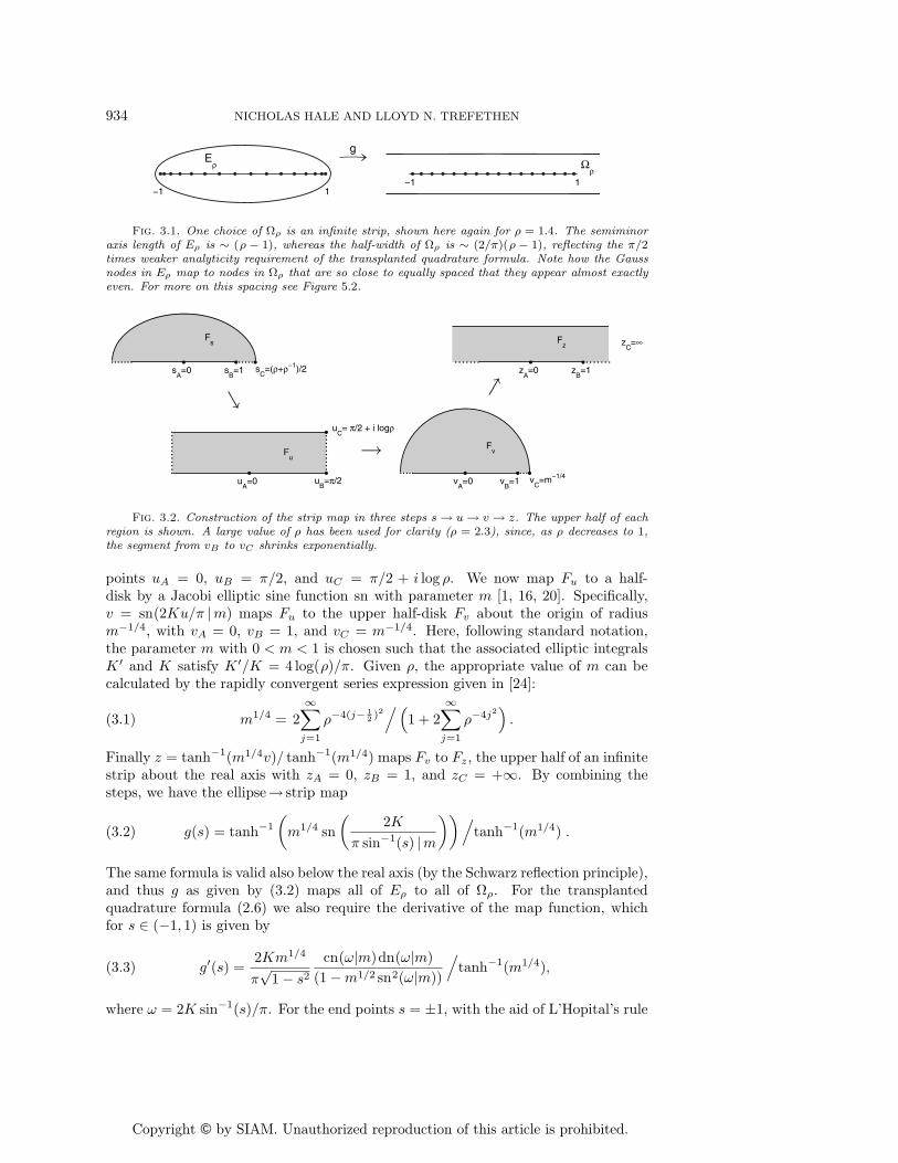
3. Map to an infinite strip. We now turn to particular choices of the map gthat may be useful in practice. Since our aim is to make the sides of Ωρ straighterthan those of Eρ, we begin by taking this notion as far as possible and consideringthe map g that takes Eρ to an infinite strip Ωρ symmetric about the real axis withg(±1) = ±1 and the ends of the ellipse mapping to ±∞ (Figure 3.1). These conditionsdetermine g fully. The half-width a of Ωρ is not adjustable but is determined by thevalue of ρ ((3.5) below).

The map of the ellipse to the strip can be constructed in three steps (Figure 3.2).Let Fs denote the upper half of Eρ, with distinguished boundary points sA = 0,sB = 1, and sC = (ρ + ρ−1)/2 (the right end point of Eρ). The function u = sin−1 smaps Fs to the rectangle Fu of width π and height log ρ with corresponding boundary



−1 1

Eρ

g

−1 1

Ωρ

Fig. 3.1. One choice of Ωρ is an infinite strip, shown here again for ρ = 1.4. The semiminoraxis length of Eρ is ∼ (ρ − 1), whereas the half-width of Ωρ is ∼ (2/π)(ρ − 1), reflecting the π/2times weaker analyticity requirement of the transplanted quadrature formula. Note how the Gaussnodes in Eρ map to nodes in Ωρ that are so close to equally spaced that they appear almost exactlyeven. For more on this spacing see Figure 5.2.

Fs

sA=0 s

B=1 s

C=(ρ+ρ−1)/2

Fu

uA=0 u

B=π/2

uC= π/2 + i logρ

Fv

vA=0 v

B=1 v

C=m−1/4

Fz

zA=0 z

B=1

zC=∞

→

→→

Fig. 3.2. Construction of the strip map in three steps s → u → v → z. The upper half of eachregion is shown. A large value of ρ has been used for clarity (ρ = 2.3), since, as ρ decreases to 1,the segment from vB to vC shrinks exponentially.

points uA = 0, uB = π/2, and uC = π/2 + i log ρ. We now map Fu to a half-disk by a Jacobi elliptic sine function sn with parameter m [1, 16, 20]. Specifically,v = sn(2Ku/π |m) maps Fu to the upper half-disk Fv about the origin of radiusm−1/4, with vA = 0, vB = 1, and vC = m−1/4. Here, following standard notation,the parameter m with 0 < m < 1 is chosen such that the associated elliptic integralsK ′ and K satisfy K ′/K = 4 log(ρ)/π. Given ρ, the appropriate value of m can becalculated by the rapidly convergent series expression given in [24]:

m1/4 = 2

∞∑j=1

ρ−4(j− 12 )2

/(1 + 2

∞∑j=1

ρ−4j2).(3.1)

Finally z = tanh−1(m1/4v)/ tanh−1(m1/4) maps Fv to Fz, the upper half of an infinitestrip about the real axis with zA = 0, zB = 1, and zC = +∞. By combining thesteps, we have the ellipse→ strip map

g(s) = tanh−1

(m1/4 sn

(2K

π sin−1(s) |m

))/tanh−1(m1/4) .(3.2)

The same formula is valid also below the real axis (by the Schwarz reflection principle),and thus g as given by (3.2) maps all of Eρ to all of Ωρ. For the transplantedquadrature formula (2.6) we also require the derivative of the map function, whichfor s ∈ (−1, 1) is given by

g′(s) =2Km1/4

π√

1 − s2

cn(ω|m)dn(ω|m)

(1 −m1/2 sn2(ω|m))

/tanh−1(m1/4),(3.3)

where ω = 2K sin−1(s)/π. For the end points s = ±1, with the aid of L’Hopital’s rule



g

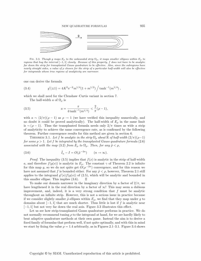
Fig. 3.3. Though g maps Eρ to the unbounded strip Ωρ, it maps smaller ellipses within Eρ toregions that hug the interval [−1, 1] closely. Because of this property, f does not have to be analyticfar down the strip for transplanted Gauss quadrature to be effective. Also, since the subregions havenearly straight sides, a value of ρ chosen for the strip of a particular half-width will also be effectivefor integrands whose true regions of analyticity are narrower.

one can derive the formula

g′(±1) = 4K2π−2m1/4(1 + m1/2)/

tanh−1(m1/4) ,(3.4)

which we shall need for the Clenshaw–Curtis variant in section 7.The half-width a of Ωρ is

a =π

4 tanh−1(m1/4)<

2

π(ρ− 1),(3.5)

with a ∼ (2/π)(ρ − 1) as ρ → 1 (we have verified this inequality numerically, andno doubt it could be proved analytically). The half-width of Eρ in the same limitis ∼ (ρ − 1). Thus the transplanted formula needs only 2/π times as wide a stripof analyticity to achieve the same convergence rate, as is confirmed by the followingtheorem. Further convergence results for this method are given in section 6.

Theorem 3.1. Let f be analytic in the strip Ωρ about R of half-width (2/π)(ρ−1)for some ρ > 1. Let f be integrated by the transplanted Gauss quadrature formula (2.6)associated with the map (3.2) from Eρ to Ωρ. Then, for any ρ < ρ,

In − I = O(ρ−2n) (n → ∞).(3.6)

Proof. The inequality (3.5) implies that f(x) is analytic in the strip of half-widtha, and therefore f(g(s)) is analytic in Eρ. The constant γ of Theorem 2.2 is infinitefor this map g, so we do not quite get O(ρ−2n) convergence, and for this reason wehave not assumed that f is bounded either. For any ρ < ρ, however, Theorem 2.1 stillapplies to the integrand g′(s)f(g(s)) of (2.5), which will be analytic and bounded inthis smaller ellipse. This implies (3.6).

To make our domain narrower in the imaginary direction by a factor of 2/π, wehave lengthened it in the real direction by a factor of ∞! This may seem a dubiousimprovement, and, indeed, it is a very strong condition that f must be analyticthroughout an infinite strip. However, this is not a serious issue in practice becauseif we consider slightly smaller ρ-ellipses within Eρ, we find that they map under g todomains about [−1, 1] that are much shorter. Thus little is lost if f is analytic near[−1, 1] but not very far down the real axis. Figure 3.3 illustrates this effect.

Let us see how strip-transplanted Gauss quadrature performs in practice. We donot normally recommend tuning ρ to the integrand at hand, for we are hardly likely tobeat adaptive quadrature methods at their own game. Instead the aim is to derive afixed family of formulas that perform well, if not quite optimally, and with this in mindwe start by fixing the value ρ = 1.4 arbitrarily, as in Figures 2.1–3.1. Figure 3.4 shows



0 10 20 30 40

10−6

10−3

100

(1+20x2 ) −1

0 10 20 30 40

10−4

10−2

100

log(1+50x2 )

0 10 20 30 4010

−6

10−4

10−2

100

(1.5−cos(5x)) −1

0 10 20 30 4010

−15

10−10

10−5

100

exp(−40x2 )

0 10 20 30 4010

−15

10−10

10−5

100

cos(40x)

0 10 20 30 40

10−6

10−3

100

exp(−x −2 )

0 10 20 30 40

10−4

10−2

100

|x|−|x−0.1|

0 10 20 30 40

10−6

10−3

100

(1.01−x)1/2

0 10 20 30 40

10−12

10−6

100

cos(x)

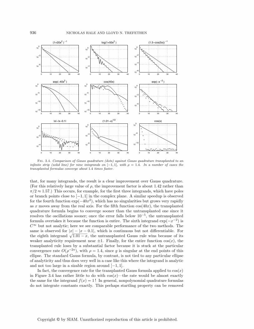
Fig. 3.4. Comparison of Gauss quadrature (dots) against Gauss quadrature transplanted to aninfinite strip (solid line) for nine integrands on [−1, 1], with ρ = 1.4. In a number of cases thetransplanted formulas converge about 1.4 times faster.

that, for many integrands, the result is a clear improvement over Gauss quadrature.(For this relatively large value of ρ, the improvement factor is about 1.42 rather thanπ/2 ≈ 1.57.) This occurs, for example, for the first three integrands, which have polesor branch points close to [−1, 1] in the complex plane. A similar speedup is observedfor the fourth function exp(−40x2), which has no singularities but grows very rapidlyas x moves away from the real axis. For the fifth function cos(40x), the transplantedquadrature formula begins to converge sooner than the untransplanted one since itresolves the oscillations sooner; once the error falls below 10−5, the untransplantedformula overtakes it because the function is entire. The sixth integrand exp(−x−2) isC∞ but not analytic; here we see comparable performance of the two methods. Thesame is observed for |x| − |x − 0.1|, which is continuous but not differentiable. Forthe eighth integrand

√1.01 − x, the untransplanted Gauss rule wins because of its

weaker analyticity requirement near ±1. Finally, for the entire function cos(x), thetransplanted rule loses by a substantial factor because it is stuck at the particularconvergence rate O(ρ−2n), with ρ = 1.4, since g is singular at the end points of thisellipse. The standard Gauss formula, by contrast, is not tied to any particular ellipseof analyticity and thus does very well in a case like this where the integrand is analyticand not too large in a sizable region around [−1, 1].

In fact, the convergence rate for the transplanted Gauss formula applied to cos(x)in Figure 3.4 has rather little to do with cos(x)—the rate would be almost exactlythe same for the integrand f(x) = 1 ! In general, nonpolynomial quadrature formulasdo not integrate constants exactly. This perhaps startling property can be removed



by a scaling adjustment to our formula (2.6), whereby we multiply the weights wk bya constant so as to make them sum to 2. Since the transplanted quadrature formulaintegrates the constant function with exponential accuracy, the adjustment factor willbe exponentially close to 1, and there will be no effect on the asymptotic convergencerates of Theorem 3.6 or Theorems 6.1 and 6.2 to follow. As a practical matter, theadjustment sometimes improves the behavior of our formulas slightly, and perhaps itis worth making.1

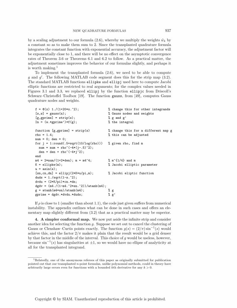
To implement the transplanted formula (2.6), we need to be able to computeg and g′. The following MATLAB code segment does this for the strip map (3.2).The standard MATLAB functions ellipke and ellipj used here to compute Jacobielliptic functions are restricted to real arguments; for the complex values needed inFigures 3.1 and 3.3, we replaced ellipj by the function ellipjc from Driscoll’sSchwarz–Christoffel Toolbox [19]. The function gauss, from [49], computes Gaussquadrature nodes and weights.

f = @(x) 1./(1+20*x.^2); % change this for other integrands

[s,w] = gauss(n); % Gauss nodes and weights

[g,gprime] = strip(s); % g and g’

In = (w.*gprime’)*f(g); % the integral

function [g,gprime] = strip(s) % change this for a different map g

rho = 1.4; % this can be adjusted

num = 0; den = 0;

for j = 1:round(.5+sqrt(10/log(rho))) % given rho, find m

num = num + rho^(-4*(j-.5)^2);

den = den + rho^(-4*j^2);

end

m4 = 2*num/(1+2*den); m = m4^4; % m^{1/4} and m

K = ellipke(m); % Jacobi elliptic parameter

u = asin(s);

[sn,cn,dn] = ellipj(2*K*u/pi,m); % Jacobi eliptic function

duds = 1./sqrt(1-s.^2);

dvdu = (2*K/pi)*cn.*dn;

dgdv = (m4./(1-m4.^2*sn.^2))/atanh(m4);

g = atanh(m4*sn)/atanh(m4); % g

gprime = dgdv.*dvdu.*duds; % g’

If ρ is close to 1 (smaller than about 1.1), the code just given suffers from numericalinstability. The appendix outlines what can be done in such cases and offers an ele-mentary map slightly different from (3.2) that as a practical matter may be superior.

4. A simpler conformal map. We now put aside the infinite strip and consideranother idea for selecting the function g. Suppose we set out to cancel the clustering ofGauss or Clenshaw–Curtis points exactly. The function g(s) = (2/π) sin−1(s) wouldachieve this, and the factor 2/π makes it plain that the result would be a grid denserby that factor in the middle of the interval. This choice of g would be useless, however,because sin−1(s) has singularities at ±1, so we would have no ellipse of analyticity atall for the transplanted integrand.

1Relatedly, one of the anonymous referees of this paper as originally submitted for publicationpointed out that our transplanted n-point formulas, unlike polynomial methods, could in theory havearbitrarily large errors even for functions with a bounded kth derivative for any k > 0.



d = 1

d = 5

d = 9

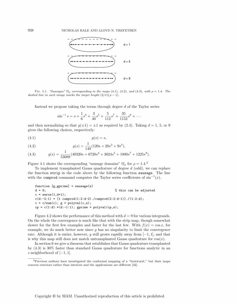
Fig. 4.1. “Sausages” Ωρ corresponding to the maps (4.1), (4.2), and (4.3), with ρ = 1.4. Thedashed line in each image marks the target height (2/π)(ρ− 1).

Instead we propose taking the terms through degree d of the Taylor series

sin−1 s = s +1

6s3 +

3

40s5 +

5

112s7 +

35

1152s9 + · · ·

and then normalizing so that g(±1) = ±1 as required by (2.4). Taking d = 1, 5, or 9gives the following choices, respectively:

g(s) = s,(4.1)

g(s) =1

149(120s + 20s3 + 9s5),(4.2)

g(s) =1

53089(40320s + 6720s3 + 3024s5 + 1800s7 + 1225s9).(4.3)

Figure 4.1 shows the corresponding “sausage domains” Ωρ for ρ = 1.4.2

To implement transplanted Gauss quadrature of degree d (odd), we can replacethe function strip in the code above by the following function sausage. The linewith the cumprod command computes the Taylor series coefficients of sin−1(x).

function [g,gprime] = sausage(s)

d = 9; % this can be adjusted

c = zeros(1,d+1);

c(d:-2:1) = [1 cumprod(1:2:d-2)./cumprod(2:2:d-1)]./(1:2:d);

c = c/sum(c); g = polyval(c,s);

cp = c(1:d).*(d:-1:1); gprime = polyval(cp,s);

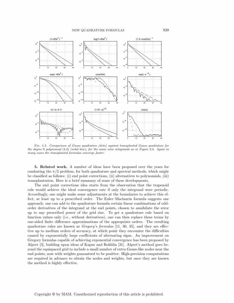
Figure 4.2 shows the performance of this method with d = 9 for various integrands.On the whole the convergence is much like that with the strip map, though somewhatslower for the first few examples and faster for the last few. With f(x) = cosx, forexample, we do much better now since g has no singularity to limit the convergencerate. Although it is entire, however, g still grows rapidly away from [−1, 1], and thatis why this map still does not match untransplanted Gauss quadrature for cos(x).

In section 6 we give a theorem that establishes that Gauss quadrature transplantedby (4.3) is 30% faster than standard Gauss quadrature for functions analytic in anε-neighborhood of [−1, 1].

2Previous authors have investigated the conformal mapping of a “bratwurst,” but their mapsconcern exteriors rather than interiors and the applications are different [32].



0 10 20 30 40

10−6

10−3

100

(1+20x2 ) −1

0 10 20 30 40

10−4

10−2

100

log(1+50x2 )

0 10 20 30 4010

−6

10−4

10−2

100

(1.5−cos(5x)) −1

0 10 20 30 4010

−15

10−10

10−5

100

exp(−40x2 )

0 10 20 30 4010

−15

10−10

10−5

100

cos(40x)

0 10 20 30 40

10−6

10−3

100

exp(−x −2 )

0 10 20 30 40

10−4

10−2

100

|x|−|x−0.1|

0 10 20 30 40

10−6

10−3

100

(1.01−x)1/2

0 10 20 30 40

10−12

10−6

100

cos(x)

Fig. 4.2. Comparison of Gauss quadrature (dots) against transplanted Gauss quadrature forthe degree 9 polynomial (4.3) (solid line), for the same nine integrands as in Figure 3.4. Again inmany cases the transplanted formulas converge faster.

5. Related work. A number of ideas have been proposed over the years forcombating the π/2 problem, for both quadrature and spectral methods, which mightbe classified as follows: (i) end point corrections, (ii) alternatives to polynomials, (iii)transplantation. Here is a brief summary of some of these developments.

The end point corrections idea starts from the observation that the trapezoidrule would achieve the ideal convergence rate if only the integrand were periodic.Accordingly, one might make some adjustments at the boundaries to achieve this ef-fect, at least up to a prescribed order. The Euler–Maclaurin formula suggests oneapproach: one can add to the quadrature formula certain linear combinations of odd-order derivatives of the integrand at the end points, chosen to annihilate the errorup to any prescribed power of the grid size. To get a quadrature rule based onfunction values only (i.e., without derivatives), one can then replace these terms byone-sided finite difference approximations of the appropriate orders. The resultingquadrature rules are known as Gregory’s formulas [11, 30, 35], and they are effec-tive up to medium orders of accuracy, at which point they encounter the difficultiescaused by exponentially large coefficients of alternating signs. An improvement onGregory formulas capable of achieving exponential convergence has been proposed byAlpert [3], building upon ideas of Kapur and Rokhlin [31]. Alpert’s method goes be-yond the equispaced grid to include a small number of extra Gauss-like nodes near theend points, now with weights guaranteed to be positive. High-precision computationsare required in advance to obtain the nodes and weights, but once they are knownthe method is highly effective.



By alternatives to polynomials we mean the explicit construction of orthogonalbases that are nonpolynomial and have more uniform behavior over the interval ofinterest. An important set of functions in this connection is the prolate spheroidalwave functions, which were introduced in the 1960s by Slepian and Pollak [45]. Thesefunctions have excellent resolution properties, and more recent authors have showntheir power for a variety of computational applications [9, 10, 13, 53]. In this literature,rather than derive theorems about convergence for functions analytic in specifieddomains as we are about to do, it is customary to quantify the matter of resolutionby considering applications to band-limited functions.

Finally there is the transplantation idea, the basis of the present article. A no-table contribution in this area is a forty-year-old theoretical paper by Bakhvalov [4].What is the optimal family of quadrature formulas, Bakhvalov asks, for the set offunctions analytic and bounded by M in a given complex region Ω containing [−1, 1]?His first step is to transplant the problem by a conformal map g to an ellipse Eρ.This is very close to what we have done but with a difference. In the ellipse, thenew quadrature problem has a weight g′. Since his aim is to investigate optimalformulas, Bakhvalov now considers the Gauss formulas associated with this weight,which he shows are in a sense optimal. By contrast we have used the unweightedGauss formula, including g′ instead as part of the integrand. We presume that thissimpler procedure does not hurt the convergence rate much in practice, but we havenot investigated this matter. Bakhvalov’s paper is full of interesting ideas, and it hasled to subsequent developments in the theoretical quadrature literature by Petras [40]and other authors [23, 28, 34]. So far as we are aware, however, this collection ofpublications has not been concerned with the π/2 phenomenon, nor with particularchoices of Ω, and does not propose actual quadrature formulas for numerical use.

A more practically oriented transplantation idea was introduced in the spectralmethods literature by Kosloff and Tal-Ezer in 1993 [33]. Like the conformal mapsproposed in the last section, the Kosloff–Tal-Ezer map is derived from the inversesine function. Their transformation is

g(s) =sin−1(αs)

sin−1(α)(5.1)

for a value of α slightly less than 1. Various methods for choosing α are consideredboth in their original paper and in various subsequent works by other authors [2, 7,15, 18, 29, 37].

The Kosloff–Tal-Ezer map is quite different from those of sections 3 and 4 inoriginal concept but rather similar in practice. These authors, and their successors,do not consider g as a conformal map, and they do not present theorems aboutgeometric rates of convergence for analytic functions. Nevertheless the function (5.1)has the familiar effect of mapping Eρ to a region with straighter sides, with the usualconsequence that the nodes are distributed more evenly in the interior and clusteredless near ±1. To investigate a Kosloff–Tal-Ezer map in the framework established inthis paper, we might begin by setting ρ = 1.4 and drawing a plot analogous to thoseof Figures 2.1, 3.1, and 4.1. The largest choice of α for which g will be analytic in Eρ

is α = 2/(ρ + ρ−1) ≈ 0.9459. Figure 5.1 shows the result.3

The node spacings for the various transformations we have considered are shown(for n = 24) in Figure 5.2.

3In [29] Hesthaven, Dinesen, and Lynov consider a spectral method with α = cos(1/2) ≈ 0.88,corresponding to ρ ≈ 1.69. In most other spectral methods papers that make use of the Kosloff–Tal-Ezer mapping, α is chosen to increase toward 1 as n increases.



−1 1

Eρ

g

−1 1

Ωρ

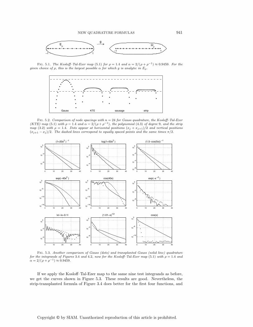
Fig. 5.1. The Kosloff–Tal-Ezer map (5.1) for ρ = 1.4 and α = 2/(ρ + ρ−1) ≈ 0.9459. For thegiven choice of ρ, this is the largest possible α for which g is analytic in Eρ.

Gauss KTE sausage strip

Fig. 5.2. Comparison of node spacings with n = 24 for Gauss quadrature, the Kosloff–Tal-Ezer(KTE) map (5.1) with ρ = 1.4 and α = 2/(ρ + ρ−1), the polynomial (4.3) of degree 9, and the stripmap (3.2) with ρ = 1.4. Dots appear at horizontal positions (xj + xj+1)/2 and vertical positions(xj+1 − xj)/2. The dashed lines correspond to equally spaced points and the same times π/2.

0 10 20 30 40

10−6

10−3

100

(1+20x2 ) −1

0 10 20 30 40

10−4

10−2

100

log(1+50x2 )

0 10 20 30 4010

−6

10−4

10−2

100

(1.5−cos(5x)) −1

0 10 20 30 4010

−15

10−10

10−5

100

exp(−40x2 )

0 10 20 30 4010

−15

10−10

10−5

100

cos(40x)

0 10 20 30 40

10−6

10−3

100

exp(−x −2 )

0 10 20 30 40

10−4

10−2

100

|x|−|x−0.1|

0 10 20 30 40

10−6

10−3

100

(1.01−x)1/2

0 10 20 30 40

10−12

10−6

100

cos(x)

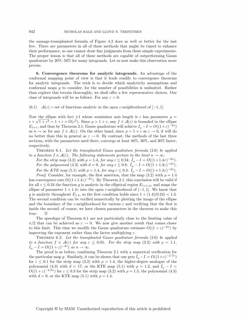
Fig. 5.3. Another comparison of Gauss (dots) and transplanted Gauss (solid line) quadraturefor the integrands of Figures 3.4 and 4.2, now for the Kosloff–Tal-Ezer map (5.1) with ρ = 1.4 andα = 2/(ρ + ρ−1) ≈ 0.9459.

If we apply the Kosloff–Tal-Ezer map to the same nine test integrands as before,we get the curves shown in Figure 5.3. These results are good. Nevertheless, thestrip-transplanted formula of Figure 3.4 does better for the first four functions, and



the sausage-transplanted formula of Figure 4.2 does as well or better for the lastfive. There are parameters in all of these methods that might be tuned to enhancetheir performance, so one cannot draw fine judgments from these simple experiments.The proper lesson is that all of these methods are capable of outperforming Gaussquadrature by 20%–50% for many integrands. Let us now make this observation moreprecise.

6. Convergence theorems for analytic integrands. An advantage of theconformal mapping point of view is that it leads readily to convergence theoremsfor analytic integrands. The trick is to decide which analyticity assumptions andconformal maps g to consider, for the number of possibilities is unlimited. Ratherthan explore this terrain thoroughly, we shall offer a few representative choices. Ourclass of integrands will be as follows. For any ε > 0:

A(ε) = set of functions analytic in the open ε-neighborhood of [−1, 1].(6.1)

Now the ellipse with foci ±1 whose semiminor axis length is ε has parameter ρ =ε +

√1 + ε2 = 1 + ε + O(ε2). Since ρ > 1 + ε, any f ∈ A(ε) is bounded in the ellipse

E1+ε, and thus by Theorem 2.1, Gauss quadrature will achieve In−I = O((1+ε)−2n)as n → ∞ for any f ∈ A(ε). On the other hand, since ρ ∼ 1 + ε as ε → 0, it will dono better than this in general as ε → 0. By contrast, the methods of the last threesections, with the parameters used there, converge at least 40%, 30%, and 30% faster,respectively.

Theorem 6.1. Let the transplanted Gauss quadrature formula (2.6) be appliedto a function f ∈ A(ε). The following statements pertain to the limit n → ∞:

For the strip map (3.2) with ρ = 1.4, for any ε ≤ 0.24: In−I = O((1+1.4ε)−2n).For the polynomial (4.3) with d = 9, for any ε ≤ 0.8: In − I = O((1 + 1.3ε)−2n).

For the KTE map (5.1) with ρ = 1.4, for any ε ≤ 0.3: In− I = O((1+1.3ε)−2n).Proof. Consider, for example, the first assertion, that the map (3.2) with ρ = 1.4

has convergence rate O((1+1.4ε)−2n). By Theorem 2.1, this conclusion will be valid iffor all ε ≤ 0.24 the function g is analytic in the elliptical region E1+1.4ε and maps theellipse of parameter 1 + 1.4ε into the open ε-neighborhood of [−1, 1]. We know thatg is analytic throughout E1.4, so the first condition holds since 1 + (1.4)(0.24) < 1.4.The second condition can be verified numerically by plotting the image of the ellipseand the boundary of the ε-neighborhood for various ε and verifying that the first isinside the second; of course, we have chosen parameters in the theorem to make thistrue.

The speedups of Theorem 6.1 are not particularly close to the limiting value ofπ/2 that can be achieved as ε → 0. We now give another result that comes closerto this limit. This time we modify the Gauss quadrature estimate O((1 + ε)−2n) byimproving the exponent rather than the factor multiplying ε.

Theorem 6.2. Let the transplanted Gauss quadrature formula (2.6) be appliedto a function f ∈ A(ε) for any ε ≤ 0.05. For the strip map (3.2) with ρ = 1.1,In − I = O((1 + ε)−3n) as n → ∞.

The proof is as before, combining Theorem 2.1 with a numerical verification forthe particular map g. Similarly, it can be shown that one gets In−I = O((1+ε)−2.7n)for ε ≤ 0.1 for the strip map (3.2) with ρ = 1.4, the higher-degree analogue of thepolynomial (4.3) with d = 17, or the KTE map (5.1) with ρ = 1.2, and In − I =O((1 + ε)−2.5n) for ε ≤ 0.3 for the strip map (3.2) with ρ = 1.5, the polynomial (4.3)with d = 9, or the KTE map (5.1) with ρ = 1.4.



7. Clenshaw–Curtis variant. Among polynomial quadrature methods, Gaussquadrature is optimal from the point of view of degree of polynomials integratedexactly, namely, 2n−1 for the formula (2.2). It also has an elegant convergence theoryfor analytic integrands, as represented by Theorem 2.1 and the further theorems wehave derived from it. Thus it is natural that, in the experiments of this paper untilnow, we have considered Gauss quadrature and its transplanted alternatives.

Gauss quadrature has the disadvantage, however, that it takes O(n2) work andmemory to compute Gauss nodes and weights by the standard algorithm of Golub andWelsch [27]. In some applications this is not an issue, because either n is small or thenodes and weights are precomputed. In others, it is troublesome indeed. Certainlyone would rarely use a Gauss quadrature formula with thousands of points.

An easy alternative is Clenshaw–Curtis quadrature, which is readily implementedvia the fast Fourier transform in O(n log n) operations [14, 26]; now there is no problemif n is 104 or 105 [6, 50]. All of the conformal transplantation ideas discussed in thisarticle can be applied to Clenshaw–Curtis as well as Gauss formulas, with comparableeffect: a speedup for many integrands by a factor approaching π/2. A Clenshaw–Curtis code segment for (n+ 1)-point integration of f over [−1, 1] can be written likethis [50]:

s = cos((0:n)’*pi/n);

[g,gprime] = strip(s);

fx = f(g).*gprime/(2*n);

h = real(fft(fx([1:n+1 n:-1:2])));

a = [h(1); h(2:n)+h(2*n:-1:n+2); h(n+1)];

w = 0*a’; w(1:2:end) = 2./(1-(0:2:n).^2);

In = w*a;

One’s first expectation is that Clenshaw–Curtis convergence rates should generallybe about half those of Gauss, for both the pure and the transplanted variants. Forexample, the n-point Clenshaw–Curtis formula exactly integrates polynomials only upto degree n, not 2n− 1, and similarly, a result like Theorem 2.1 holds with O(ρ−2n)reduced to O(ρ−n). Thus one might expect that a transplanted Clenshaw–Curtisformula should converge about 2× 2/π = 4/π times more slowly than untransplantedGauss quadrature.

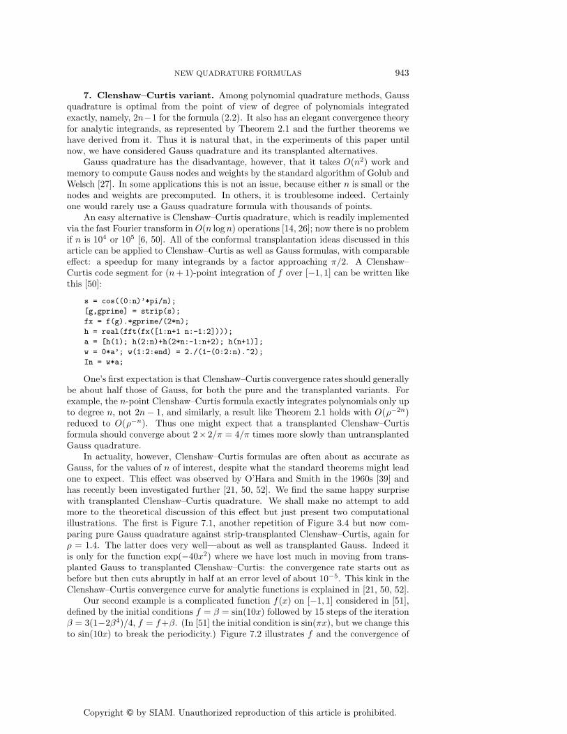
In actuality, however, Clenshaw–Curtis formulas are often about as accurate asGauss, for the values of n of interest, despite what the standard theorems might leadone to expect. This effect was observed by O’Hara and Smith in the 1960s [39] andhas recently been investigated further [21, 50, 52]. We find the same happy surprisewith transplanted Clenshaw–Curtis quadrature. We shall make no attempt to addmore to the theoretical discussion of this effect but just present two computationalillustrations. The first is Figure 7.1, another repetition of Figure 3.4 but now com-paring pure Gauss quadrature against strip-transplanted Clenshaw–Curtis, again forρ = 1.4. The latter does very well—about as well as transplanted Gauss. Indeed itis only for the function exp(−40x2) where we have lost much in moving from trans-planted Gauss to transplanted Clenshaw–Curtis: the convergence rate starts out asbefore but then cuts abruptly in half at an error level of about 10−5. This kink in theClenshaw–Curtis convergence curve for analytic functions is explained in [21, 50, 52].

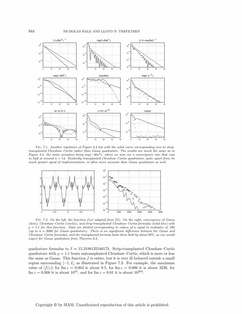
Our second example is a complicated function f(x) on [−1, 1] considered in [51],defined by the initial conditions f = β = sin(10x) followed by 15 steps of the iterationβ = 3(1−2β4)/4, f = f+β. (In [51] the initial condition is sin(πx), but we change thisto sin(10x) to break the periodicity.) Figure 7.2 illustrates f and the convergence of



0 10 20 30 40

10−6

10−3

100

(1+20x2 ) −1

0 10 20 30 40

10−4

10−2

100

log(1+50x2 )

0 10 20 30 4010

−6

10−4

10−2

100

(1.5−cos(5x)) −1

0 10 20 30 4010

−15

10−10

10−5

100

exp(−40x2 )

0 10 20 30 4010

−15

10−10

10−5

100

cos(40x)

0 10 20 30 40

10−6

10−3

100

exp(−x −2 )

0 10 20 30 40

10−4

10−2

100

|x|−|x−0.1|

0 10 20 30 40

10−6

10−3

100

(1.01−x)1/2

0 10 20 30 40

10−12

10−6

100

cos(x)

Fig. 7.1. Another repetition of Figure 3.4 but with the solid curve corresponding now to strip-transplanted Clenshaw–Curtis rather than Gauss quadrature. The results are much the same as inFigure 3.4, the main exception being exp(−40x2), where we now see a convergence rate that cutsin half at around n = 14. Evidently transplanted Clenshaw–Curtis quadrature, quite apart from itsmuch greater speed of implementation, is often more accurate than Gauss quadrature as well.

−1 −0.5 0 0.5 1

6

7

8

9

0 1000 2000 3000 4000 500010

−12

10−10

10−8

10−6

10−4

10−2

100

Fig. 7.2. On the left, the function f(x) adapted from [51]. On the right, convergence of Gauss(dots), Clenshaw–Curtis (circles), and strip-transplanted Clenshaw–Curtis formulas (solid line) withρ = 1.1 for this function. Data are plotted corresponding to values of n equal to multiples of 100(up to n = 2000 for Gauss quadrature). There is no significant difference between the Gauss andClenshaw–Curtis formulas, and the transplanted formula beats them both by about 50%, as one wouldexpect for Gauss quadrature from Theorem 6.2.

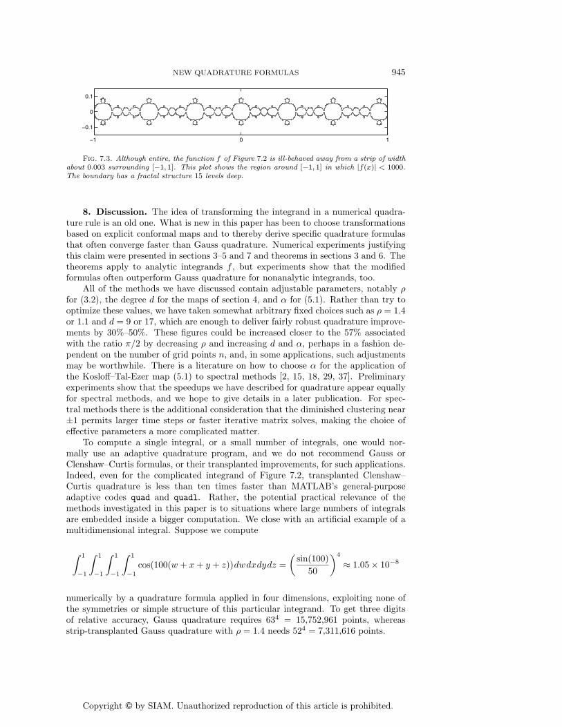
quadrature formulas to I ≈ 15.3198135546173. Strip-transplanted Clenshaw–Curtisquadrature with ρ = 1.1 beats untransplanted Clenshaw–Curtis, which is more or lessthe same as Gauss. This function f is entire, but it is very ill behaved outside a smallregion surrounding [−1, 1], as illustrated in Figure 7.3. For example, the maximumvalue of |f(z)| for Im z = 0.004 is about 9.5, for Im z = 0.006 it is about 3236, forIm z = 0.008 it is about 1041, and for Im z = 0.01 it is about 10263.



−1 0 1

−0.1

0

0.1

Fig. 7.3. Although entire, the function f of Figure 7.2 is ill-behaved away from a strip of widthabout 0.003 surrounding [−1, 1]. This plot shows the region around [−1, 1] in which |f(x)| < 1000.The boundary has a fractal structure 15 levels deep.

8. Discussion. The idea of transforming the integrand in a numerical quadra-ture rule is an old one. What is new in this paper has been to choose transformationsbased on explicit conformal maps and to thereby derive specific quadrature formulasthat often converge faster than Gauss quadrature. Numerical experiments justifyingthis claim were presented in sections 3–5 and 7 and theorems in sections 3 and 6. Thetheorems apply to analytic integrands f , but experiments show that the modifiedformulas often outperform Gauss quadrature for nonanalytic integrands, too.

All of the methods we have discussed contain adjustable parameters, notably ρfor (3.2), the degree d for the maps of section 4, and α for (5.1). Rather than try tooptimize these values, we have taken somewhat arbitrary fixed choices such as ρ = 1.4or 1.1 and d = 9 or 17, which are enough to deliver fairly robust quadrature improve-ments by 30%–50%. These figures could be increased closer to the 57% associatedwith the ratio π/2 by decreasing ρ and increasing d and α, perhaps in a fashion de-pendent on the number of grid points n, and, in some applications, such adjustmentsmay be worthwhile. There is a literature on how to choose α for the application ofthe Kosloff–Tal-Ezer map (5.1) to spectral methods [2, 15, 18, 29, 37]. Preliminaryexperiments show that the speedups we have described for quadrature appear equallyfor spectral methods, and we hope to give details in a later publication. For spec-tral methods there is the additional consideration that the diminished clustering near±1 permits larger time steps or faster iterative matrix solves, making the choice ofeffective parameters a more complicated matter.

To compute a single integral, or a small number of integrals, one would nor-mally use an adaptive quadrature program, and we do not recommend Gauss orClenshaw–Curtis formulas, or their transplanted improvements, for such applications.Indeed, even for the complicated integrand of Figure 7.2, transplanted Clenshaw–Curtis quadrature is less than ten times faster than MATLAB’s general-purposeadaptive codes quad and quadl. Rather, the potential practical relevance of themethods investigated in this paper is to situations where large numbers of integralsare embedded inside a bigger computation. We close with an artificial example of amultidimensional integral. Suppose we compute

∫ 1

−1

∫ 1

−1

∫ 1

−1

∫ 1

−1

cos(100(w + x + y + z))dwdxdydz =

(sin(100)

50

)4

≈ 1.05 × 10−8

numerically by a quadrature formula applied in four dimensions, exploiting none ofthe symmetries or simple structure of this particular integrand. To get three digitsof relative accuracy, Gauss quadrature requires 634 = 15,752,961 points, whereasstrip-transplanted Gauss quadrature with ρ = 1.4 needs 524 = 7,311,616 points.



Appendix. Computation of the strip transformation in extreme casesand a MATLAB code. Figure 3.2 shows how the conformal map g of (3.2) from theρ-ellipse Eρ to the infinite strip Ωρ can be constructed in three steps: ellipse→periodicstrip→disk→infinite strip, with the middle step involving a Jacobi elliptic function.All of this is mathematically straightforward, but, when ρ is smaller than about 1.1,it is numerically troublesome. The problem is that the right end of the periodicstrip gets mapped in the disk domain to the interval [1,m−1/4], and this intervalshrinks exponentially as ρ decreases to 1 (similarly at the left end). For example,ρ = 1.4, 1.2, 1.1 correspond to m−1/4 ≈ 1.0026, 1.0000053, 1.000000000023, and forρ = 1.05 one calculates m−1/4 = 1 on a computer to machine precision. This “crowd-ing phenomenon” is a familiar challenge in numerical conformal mapping, making itimpossible to compute g accurately unless the computation is reformulated [20].

It would be possible to consider systematically the development of an algorithmto evaluate g to as close to machine precision as possible. Rather than attempt this,we propose a method that works very well for our quadrature application and is muchsimpler. When ρ is small, the two ends of the rectangle→ strip map of Figure 3.2are exponentially decoupled from one another. In fact, for ρ less than about 1.2, themap near one end of the rectangle is indistinguishable in 16-digit arithmetic fromwhat it would be if the rectangle were a semi-infinite strip. By following this line ofreasoning, after quite of bit of algebra, one is led to consider the function g definedby u = sin−1 s, τ = π/ log ρ, and

g(s) = C

[log(1 + e−τ(π/2+u)) − log(1 + e−τ(π/2−u)) +

(1

2+

1

eτπ + 1

)τu

],(A.1)

where the constant C is fixed so that g(±1) = ±1. To 16-digit precision, for ρ < 1.2,this function is the same as the strip map (3.2); and it is numerically reliable downto about ρ = 1.02, which is closer to 1 than one would ever need to go in practice.For s ∈ (−1, 1) the derivative is

g′(s) =−τC√1 − s2

[1

eτ(π/2+u) + 1+

1

eτ(π/2−u) + 1−(

1

2+

1

eτπ + 1

)],(A.2)

and at the end points we have

g′(±1) =Cτ2

4tanh2

(τπ2

).(A.3)

Notice how much more elementary (A.1)–(A.2) are than (3.1)–(3.4). In principle g isnot analytic in the ellipse, having branch points at s = ±1. The singularities are soweak, however, that for ρ < 1.2 they are undetectable in 16-digit arithmetic.

Although the map (A.1) was derived as an approximation to the ideal (3.2) forsmall values of ρ, it is surprisingly effective even for larger values of ρ. If (3.2) isreplaced by (A.1) in the experiments of Figure 3.4, for example, it makes no difference.

The following terse code combines all of the elements we have discussed, imple-menting the Clenshaw–Curtis quadrature formula for the modified strip transforma-tion (A.1). Since such a code will be especially useful for large n, the listing givesa value of ρ close to 1. If this code is applied to the function of Figure 7.2 withn = 1800, it gets the right answer to 15 digits in about 0.01 seconds on a 2006 work-station. (With n = 106 it gets the same answer in 5 seconds.) Untransformed Gaussquadrature with n = 1800 achieves 11 digits of accuracy and takes far longer.



function I = CCstrip(f,n) % transplanted C-C quad.

rho = 1.1; t = pi/log(rho); % rho (adjustable) and tau

d = .5+1/(exp(t*pi)+1); p2 = pi/2; % convenient abbreviations

up = pi*(0:n)/n; u = up-p2; um = p2-u; % u and shifts by +-pi/2

C = 1/(log(1+exp(-t*pi))-log(2)+p2*t*d);

g = C*(log(1+exp(-t*up))-log(1+exp(-t*um))+u*t*d); % map g

gp = 1./(exp(t*up)+1)+1./(exp(t*um)+1)-d;

gp(2:n) = -t*C*gp(2:n)./cos(u(2:n));

gp([1 n+1]) = C*(t*tanh(p2*t)/2)^2; % derivative g’

fx = f(g).*gp/(2*n); % transplanted integrand

h = real(fft(fx([1:n+1 n:-1:2]))); % Chebyshev coefficients

a = [h(1) h(2:n)+h(2*n:-1:n+2) h(n+1)];

w = 0*a; w(1:2:n+1) = 2./(1-(0:2:n).^2); % Clenshaw-Curtis weights

I = w*a’; % the result

Acknowledgments. We are grateful for helpful suggestions to Gregory Beylkin,Adam Chandler, Toby Driscoll, Christian Lubich, Ricardo Pachon, and AndreWeideman.

REFERENCES

[1] M. Abramowitz and I. A. Stegun, Handbook of Mathematical Functions, Dover, New York,1972 (originally published in 1964).

[2] M. R. Abril-Raymundo and B. Garcia-Archilla, Approximation properties of a mappedChebyshev method, Appl. Numer. Math., 32 (2000), pp. 119–136.

[3] B. K. Alpert, Hybrid Gauss-trapezoidal quadrature rules, SIAM J. Sci. Comput., 20 (1999),pp. 1551–1584.

[4] N. S. Bakhvalov, On the optimal speed of integrating analytic functions, Comput. Math.Math. Phys., 7 (1967), pp. 63–75.

[5] W. Barrett, On the convergence of Cotes’ quadrature formulae, J. London Math. Soc., 39(1964), pp. 296–302.

[6] Z. Battles and L. N. Trefethen, An extension of MATLAB to continuous functions andoperators, SIAM J. Sci. Comput., 25 (2004), pp. 1743–1770.

[7] A. Bayliss and E. Turkel, Mappings and accuracy for Chebyshev pseudo-spectral approxi-mations, J. Comput. Phys., 101 (1992), pp. 349–359.

[8] S. Bernstein, Quelques remarques sur l’interpolation, Math. Ann., 79 (1919), pp. 1–12.[9] G. Beylkin and K. Sandberg, Wave propagation using bases for bandlimited functions, Wave

Motion, 41 (2005), pp. 263–291.[10] J. P. Boyd, Prolate spheroidal wavefunctions as an alternative to Chebyshev and Legendre

polynomials for spectral element and pseudospectral algorithms, J. Comput. Phys., 199(2004), pp. 688–716.

[11] H. Brass, Quadraturverfahren, Vandenhoeck and Ruprecht, Gottingen, 1977.[12] C. Canuto, M. Y. Hussaini, A. Quarteroni, and T. A. Zang, Spectral Methods: Funda-

mentals in Single Domains, Springer, New York, 2006.[13] Q. Y. Chen, D. Gottlieb, and J. S. Hesthaven, Spectral methods based on prolate spheroidal

wave functions for hyperbolic PDEs, SIAM J. Numer. Anal., 43 (2005), pp. 1912–1933.[14] C. W. Clenshaw and A. R. Curtis, A method for numerical integration on an automatic

computer, Numer. Math., 2 (1960), pp. 197–205.[15] B. Costa, W. S. Don, and A. Simas, Exponential Convergence of Mapped Chebyshev Methods,

manuscript, 2007.[16] P. J. Davis and P. Rabinowitz, Methods of Numerical Integration, 2nd ed., Academic Press,

New York, 1984.[17] Z. Ditzian and V. Totik, Moduli of Smoothness, Springer, New York, 1987.[18] W.-S. Don and A. Solomonoff, Accuracy enhancement for higher derivatives using Cheby-

shev collocation and a mapping technique, SIAM J. Sci. Comput., 18 (1997), pp. 1040–1055.[19] T. A. Driscoll, Algorithm 843: Improvements to the MATLAB toolbox for Schwarz–

Christoffel mapping, ACM Trans. Math. Software, 31 (2005), pp. 239–251.[20] T. A. Driscoll and L. N. Trefethen, Schwarz–Christoffel Mapping, Cambridge University

Press, London, 2002.



[21] D. Elliott, B. M. Johnston, and P. R. Johnston, Clenshaw–Curtis and Gauss-LegendreQuadrature for Certain Boundary Element Integrals, manuscript, 2006.

[22] H. Engels, Numerical Quadrature and Cubature, Academic Press, London, 1980.[23] P. Favati, G. Lotti, and F. Romani, Bounds on the error of Fejer and Clenshaw–Curtis type

quadrature for analytic functions, Appl. Math. Lett., 6 (1993), pp. 3–8.[24] H. E. Fettis, Note on the computation of Jacobi’s nome and its inverse, Computing, 4 (1969),

pp. 202–206.[25] W. Gautschi, A Survey of Gauss–Christoffel Quadrature Formulae, E. B. Christoffel, P. L.

Butzer and F. Feher, eds., Birkhauser, Basel, 1981, pp. 72–147.[26] W. M. Gentleman, Implementing Clenshaw–Curtis quadrature I and II, Comm. ACM, 15

(1972), pp. 337–346, 353.[27] G. H. Golub and J. H. Welsch, Calculation of Gauss quadrature rules, Math. Comp., 23

(1969), pp. 221–230.[28] M. Gotz, Optimal quadrature for analytic functions, J. Comput. Appl. Math., 137 (2001),

pp. 123–133.[29] J. S. Hesthaven, P. G. Dinesen, and J. P. Lynov, Spectral collocation time-domain modelling

of diffractive optical elements, J. Comput. Phys., 155 (1999), pp. 287–306.[30] F. B. Hildebrand, Introduction to Numerical Analysis, 2nd ed., Dover, New York, 1987 (orig-

inally published in 1974).[31] S. Kapur and V. Rokhlin, High-order corrected trapezoidal quadrature rules for singular

functions, SIAM J. Numer. Anal., 34 (1997), pp. 1331–1356.[32] T. Koch and J. Liesen, The conformal ‘bratwurst’ maps and associated Faber polynomials,

Numer. Math., 86 (2000), pp. 173–191.[33] D. Kosloff and H. Tal-Ezer, A modified Chebyshev pseudospectral method with an O(N−1)

time step restriction, J. Comput. Phys., 104 (1993), pp. 457–469.[34] M. A. Kowalski, A. G. Werschulz, and H. Wozniakowski, Is Gauss quadrature optimal

for analytic functions?, Numer. Math., 47 (1985), pp. 89–98.[35] E. Martensen, Optimale Fehlerschranken fuer die Quadraturformel von Gregory, Z. Angew.

Math. Mech., 44 (1964), pp. 159–168.[36] V. I. Krylov, Approximate Calculation of Integrals, Dover, New York, 2005 (originally pub-

lished in 1962).[37] J. L. Mead and R. A. Renaut, Accuracy, resolution, and stability properties of a modified

Chebyshev method, SIAM J. Sci. Comput., 24 (2002), pp. 143–160.[38] M. Mori and M. Sugihara, The double-exponential transformation in numerical analysis, J.

Comput. Appl. Math., 127 (2001), pp. 287–296.[39] H. O’Hara and F. J. Smith, Error estimation in the Clenshaw–Curtis quadrature formula,

Computer J., 11 (1968), pp. 213–219.[40] K. Petras, Gaussian versus optimal integration of analytic functions, Constr. Approx., 14

(1998), pp. 231–245.[41] G. Polya, Uber die Konvergenz von Quadraturverfahren, Math. Z., 37 (1933), pp. 264–286.[42] P. Rabinowitz, Rough and ready error estimates in Gaussian integration of analytic functions,

Comm. ACM, 12 (1969), pp. 268–270.[43] T. W. Sag and G. Szekeres, Numerical evaluation of high-dimensional integrals, Math.

Comp., 18 (1964), pp. 245–253.[44] C. Schwartz, Numerical integration of analytic functions, J. Comput. Phys., 4 (1969), pp. 19–

29.[45] D. Slepian and H. O. Pollak, Prolate spheroidal wave functions, Fourier analysis and un-

certainty. I, Bell System Tech. J., 40 (1961), pp. 43–63.[46] F. Stenger, Numerical Methods Based on Sinc and Analytic Functions, Springer, New York,

1993.[47] H. Takahasi and M. Mori, Double exponential formulas for numerical integration, Publ. Res.

Inst. Math. Sci., 9 (1974), pp. 721–741.[48] T. W. Tee and L. N. Trefethen, A rational spectral collocation method with adaptively

transformed Chebyshev grid points, SIAM J. Sci. Comput., 28 (2006), pp. 1798–1811.[49] L. N. Trefethen, Spectral Methods in MATLAB, SIAM, Philadelphia, 2001.[50] L. N. Trefethen, Is Gauss quadrature better than Clenshaw–Curtis?, SIAM Rev., 50 (2008),

pp. 67–87.[51] L. N. Trefethen, Computing numerically with functions instead of numbers, Math. Comput.

Sci., 1 (2007), pp. 9–19.[52] J. A. C. Weideman and L. N. Trefethen, The kink phenomenon in Fejer and Clenshaw–

Curtis quadrature, Numer. Math., 107 (2007), pp. 707–727.[53] H. Xiao, V. Rokhlin, and N. Yarvin, Prolate spheroidal wavefunctions, quadrature and

interpolation, Inverse Problems, 17 (2001), pp. 805–838.

Documents

NEW QUADRATURE FORMULAS FROM …people.maths.ox.ac.uk/trefethen/publication/PDF/2008_128.pdfNEW QUADRATURE FORMULAS FROM CONFORMAL MAPS AND ... ANAL. c 2008 Society for Industrial