New Time and Multipath Augmentations for the Global

New Time and Multipath Augmentations for the Global

Positioning System

by

John A. Pratt

B.S., Utah State University, 2009

M.S., Utah State University, 2009

A thesis submitted to the

Faculty of the Graduate School of the

University of Colorado in partial fulfillment

of the requirements for the degree of

Doctor of Philosophy

Department of Aerospace Engineering Sciences

2015

This thesis entitled:New Time and Multipath Augmentations for the Global Positioning System

written by John A. Pratthas been approved for the Department of Aerospace Engineering Sciences

Dr. Kristine Larson

Dr. Penina Axelrad

Date

The final copy of this thesis has been examined by the signatories, and we find that both thecontent and the form meet acceptable presentation standards of scholarly work in the above

mentioned discipline.

iii

Pratt, John A. (Ph.D., Aerospace Engineering Sciences)

New Time and Multipath Augmentations for the Global Positioning System

Thesis directed by Dr. Kristine Larson

Although developed with a narrow focus in mind, use of GPS has expanded into dozens

of fields in industry, science, and military applications. The purpose of the research detailed in

this dissertation is an increase in the utility of GPS by improving primary applications of the

constellation and expand the practicality of some secondary applications. The first portion of this

disseration focuses on the development of clock estimation algorithms for a GPS aiding system

called iGPS which has been designed to improve the performance of the system in challenging

environments. Central to the functioning of iGPS are the Iridium communication satellites. This

dissertation describes a Kalman filter for estimating Iridium satellite clock biases from GPS-like

measurements at an interval of 10 s. Typical results show the current filter to be accurate to within

200 ns while always meeting the initial system specification of half a microsecond. The following

chapter examines the expediency of increasing the number of terms used to represent the clock

bias in the broadcast message and it is shown that the current broadcast message is sufficient.

The second half of the dissertation deals with the use of GPS multipath as an environmental

measurement. It is shown that reflections of GPS signals from the ground can be used to estimate

several important phenological indicators relative to the vegetation surrounding the GPS antenna.

Methods are developed for refining the reflected signal and preparing it for use as a vegetation index.

Finally, the effect of temperature and multipath supression algorithms on the GPS multipath data

is examined relative to its viability for use as previously described. It is shown that these effects

are minor in the majority of the GPS sites used in this study and that the data can be adjusted to

avoid temperature difficulties.

Dedication

For my wife and children.

v

Acknowledgements

First and foremost I would like to thank the untiring efforts of Dr. Kristine Larson and Dr.

Penina Axelrad who advised me on the different sections of my dissertation. Without their help, I

would not have been able to do this work.

I would also like to thank Dr. Richard Gerren, Nicholas DiOrio, Bruno Lesage, Dr. Eric

Small, Dr. Felipe Nievinski, and other members of the iGPS group who all provided assistance

on various aspects of my research. I am additionally grateful to my committe members: Dr. Eric

Small, Dr. Dennis Akos, and Dr. Judah Levine.

The iGPS research was sponsored by Coherent Navigation under a prime contract from Boe-

ing awarded by the Naval Research Laboratory (NRL). The author is grateful to William Bencze,

Clark Cohen, Isaac Miller, and Tom Holmes of Coherent Navigation; Misa Iovanov (Boeing) and

Mark Nelson (Kinetx) supporting Iridium Communications; Brian Patti (via Boeing subcontract)

and John Rice of Iridium Communications; Peter Fyfe, Don Tong, Rick Gerardi, and Phil Strana-

han of Boeing Defense, Space & Security; and Joseph White, Ken Senior, and High Integrity GPS

Program Manager Jay Oaks of NRL for their efforts in facilitating this work.

Funding for the broadcast clock analysis was provided by the GAANN fellowship for which

the author is very grateful.

The included multipath research was funded through NASA NNX12AK21G, NSF EAR

0948957, and NASA NNX11AL50H. Some of this material is based on data, equipment, and engi-

neering services provided by the Plate Boundary Observatory operated by UNAVCO for EarthScope

and supported by NSF (EAR-0350028 and EAR-0732947).

vi

Contents

Chapter

1 The Global Positioning System 1

1.1 GPS basics . . . . . . . . . . . . . . . . . . . . . . . . . . . . . . . . . . . . . . . . . 1

1.2 Thesis goals and chapter summary . . . . . . . . . . . . . . . . . . . . . . . . . . . . 4

2 Timing and Clocks 6

2.1 Precision clocks and the Allan Deviation . . . . . . . . . . . . . . . . . . . . . . . . . 6

2.2 Periodic variation in GPS clocks . . . . . . . . . . . . . . . . . . . . . . . . . . . . . 8

2.3 iGPS and the Iridium constellation . . . . . . . . . . . . . . . . . . . . . . . . . . . . 10

2.4 Clock Modeling and Time Scales . . . . . . . . . . . . . . . . . . . . . . . . . . . . . 12

2.5 Contributions of this work . . . . . . . . . . . . . . . . . . . . . . . . . . . . . . . . . 14

3 The improvement of the GPS broadcast clock correction by using periodic terms 16

3.1 Accuracy of the GPS Satellite Clocks . . . . . . . . . . . . . . . . . . . . . . . . . . . 16

3.2 Periodic Portion of the GPS Clock Bias . . . . . . . . . . . . . . . . . . . . . . . . . 17

3.3 GPS Clock Bias Representations . . . . . . . . . . . . . . . . . . . . . . . . . . . . . 21

3.4 Conclusions . . . . . . . . . . . . . . . . . . . . . . . . . . . . . . . . . . . . . . . . . 30

4 Estimates of iGPS satellite clocks 31

4.1 Introduction . . . . . . . . . . . . . . . . . . . . . . . . . . . . . . . . . . . . . . . . . 31

4.2 Measurement Models and Characteristics . . . . . . . . . . . . . . . . . . . . . . . . 33

vii

4.3 Clock Filters . . . . . . . . . . . . . . . . . . . . . . . . . . . . . . . . . . . . . . . . 39

4.4 Filter Results . . . . . . . . . . . . . . . . . . . . . . . . . . . . . . . . . . . . . . . . 42

4.5 Conclusions . . . . . . . . . . . . . . . . . . . . . . . . . . . . . . . . . . . . . . . . . 49

5 GPS Reflections and Phenology 51

5.1 GPS errors as measurements . . . . . . . . . . . . . . . . . . . . . . . . . . . . . . . 51

5.1.1 GPS-R . . . . . . . . . . . . . . . . . . . . . . . . . . . . . . . . . . . . . . . . 51

5.1.2 GPS-IR . . . . . . . . . . . . . . . . . . . . . . . . . . . . . . . . . . . . . . . 52

5.2 Phenology . . . . . . . . . . . . . . . . . . . . . . . . . . . . . . . . . . . . . . . . . . 54

5.2.1 Origin and Metrics . . . . . . . . . . . . . . . . . . . . . . . . . . . . . . . . . 54

6 GPS Multipath 57

6.1 Multipath basics . . . . . . . . . . . . . . . . . . . . . . . . . . . . . . . . . . . . . . 57

6.2 Measuring GPS Multipath via MP1 . . . . . . . . . . . . . . . . . . . . . . . . . . . 65

6.3 MP1 RMS . . . . . . . . . . . . . . . . . . . . . . . . . . . . . . . . . . . . . . . . . . 69

6.4 Contributions of this work . . . . . . . . . . . . . . . . . . . . . . . . . . . . . . . . . 77

7 Analysis of GPS MP1 RMS Data for Use in Vegetation Studies 78

7.1 MP1 RMS and Environmental Sensing . . . . . . . . . . . . . . . . . . . . . . . . . . 78

7.2 MP1 RMS and the PBO Network . . . . . . . . . . . . . . . . . . . . . . . . . . . . . 80

7.3 Removing Snow Effects from MP1 RMS . . . . . . . . . . . . . . . . . . . . . . . . . 82

7.4 Removing Rain Effects from MP1 RMS . . . . . . . . . . . . . . . . . . . . . . . . . 91

7.5 Hardware Effects . . . . . . . . . . . . . . . . . . . . . . . . . . . . . . . . . . . . . . 99

7.6 Removing MP1 RMS hardware based trends . . . . . . . . . . . . . . . . . . . . . . 104

7.7 Normalization . . . . . . . . . . . . . . . . . . . . . . . . . . . . . . . . . . . . . . . . 110

7.8 Published Products . . . . . . . . . . . . . . . . . . . . . . . . . . . . . . . . . . . . . 118

8 Secondary noise sources in the MP1 RMS data 120

8.1 Temperature effects on the MP1 RMS data . . . . . . . . . . . . . . . . . . . . . . . 120

viii

8.2 Multipath supression algorithms . . . . . . . . . . . . . . . . . . . . . . . . . . . . . 129

9 Summary and Future Work 133

9.1 Periodic Representations of Navigation Satellite Clocks . . . . . . . . . . . . . . . . . 133

9.2 High Integrity GPS . . . . . . . . . . . . . . . . . . . . . . . . . . . . . . . . . . . . . 133

9.3 Measurement of vegetation using MP1 RMS . . . . . . . . . . . . . . . . . . . . . . . 134

Bibliography 136

Appendix

A Explanation of the modified Allan variance 142

B Least Squares Estimation of Sine Waves 145

C Estimation of the GPS Satellite Clocks 148

D Kalman Filter Process Noise in Clock Bias Estimation 153

E MODIS 155

F Salar de Uyuni Experiment 158

ix

Figures

Figure

1.1 A GPS receiver requires data from at least four satellites in order to compute time

and position. Additional satellites can be used to improve the accuracy and precision

of the estimates. . . . . . . . . . . . . . . . . . . . . . . . . . . . . . . . . . . . . . . 2

2.1 Example modified Allan deviation of a clock with noise types noted as well as the

slope that results from that noise type. . . . . . . . . . . . . . . . . . . . . . . . . . . 8

2.2 Typical Allan deviations experienced by quartz(blue), rubidium(green), cesium beam(red),

and hydrogen maser clocks(yellow). Typical values based on figures in [Coates, 2014;

Vig, 1992; Allan et al., 1997]. . . . . . . . . . . . . . . . . . . . . . . . . . . . . . . . 9

2.3 iGPS elements and signals. iGPS uses several reference stations that receive and

process signals from both the GPS and Iridium satellites. Each reference station

uses GPS information to determine the bias in its reference clock. The central

estimator at the operations center uses the Iridium downlink and crosslink signals

to determine the Iridium satellite clock biases. . . . . . . . . . . . . . . . . . . . . . . 11

2.4 Laboratory measurements of the Allan deviation for a sample clock expected to be

representative of on-orbit performance of the Iridium satellite clocks. Sample clock

measurements courtesy of Joseph White. Typical Allan deviation ranges of rubidium

and quartz clocks are also shown for reference [Coates, 2014; Vig, 1992; Allan et al.,

1997] . . . . . . . . . . . . . . . . . . . . . . . . . . . . . . . . . . . . . . . . . . . . . 13

x

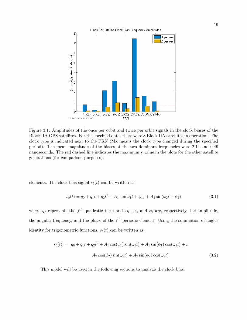
3.1 Amplitudes of the once per orbit and twice per orbit signals in the clock biases of the

Block IIA GPS satellites. For the specified dates there were 8 Block IIA satellites in

operation. The clock type is indicated next to the PRN (Mx means the clock type

changed during the specified period). The mean magnitude of the biases at the two

dominant frequencies were 2.14 and 0.49 nanoseconds. The red dashed line indicates

the maximum y value in the plots for the other satellite generations (for comparison

purposes). . . . . . . . . . . . . . . . . . . . . . . . . . . . . . . . . . . . . . . . . . . 19

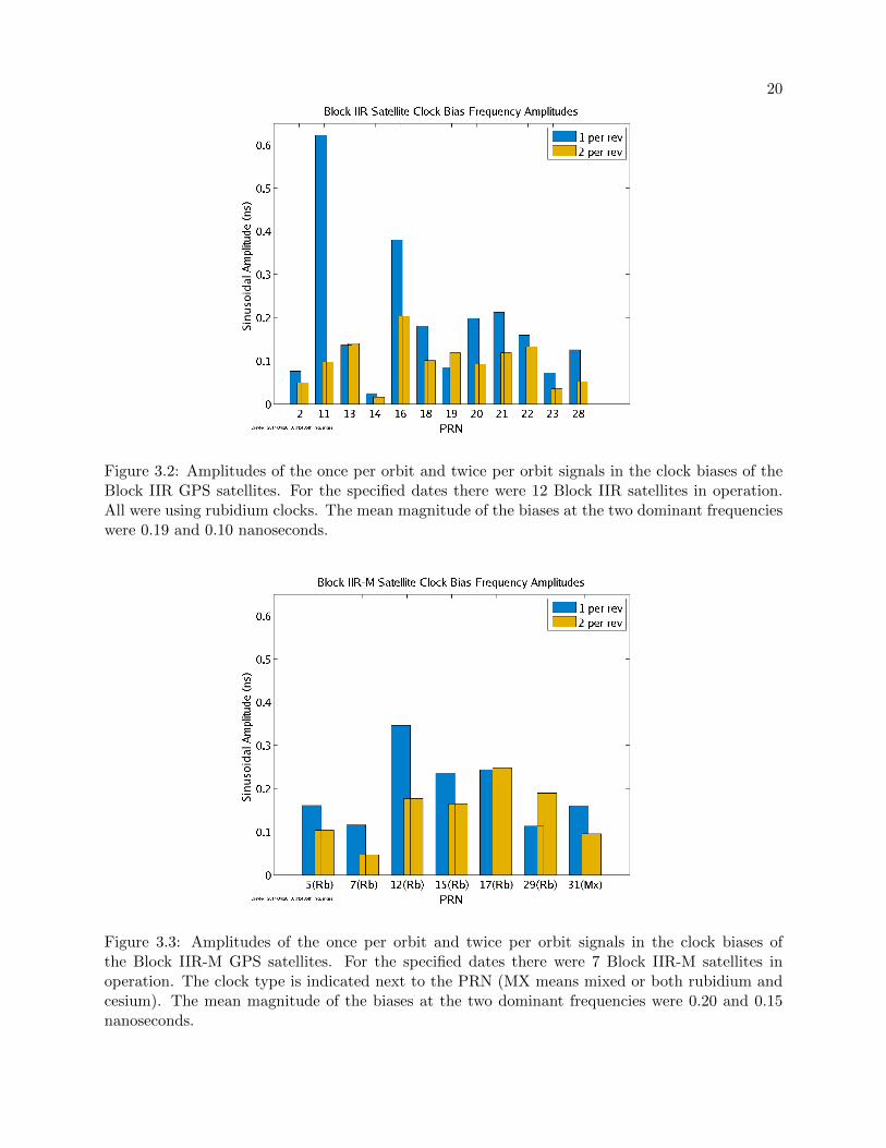
3.2 Amplitudes of the once per orbit and twice per orbit signals in the clock biases of the

Block IIR GPS satellites. For the specified dates there were 12 Block IIR satellites

in operation. All were using rubidium clocks. The mean magnitude of the biases at

the two dominant frequencies were 0.19 and 0.10 nanoseconds. . . . . . . . . . . . . 20

3.3 Amplitudes of the once per orbit and twice per orbit signals in the clock biases of

the Block IIR-M GPS satellites. For the specified dates there were 7 Block IIR-M

satellites in operation. The clock type is indicated next to the PRN (MX means

mixed or both rubidium and cesium). The mean magnitude of the biases at the two

dominant frequencies were 0.20 and 0.15 nanoseconds. . . . . . . . . . . . . . . . . . 20

3.4 Amplitudes of the once per orbit and twice per orbit signals in the clock biases

of the Block IIF GPS satellites. For the specified dates there were 2 Block IIF

satellites in operation. All Block IIF satellites will be using rubidium clocks. The

mean magnitude of the biases at the two dominant frequencies were 0.15 and 0.14

nanoseconds. . . . . . . . . . . . . . . . . . . . . . . . . . . . . . . . . . . . . . . . . 21

3.5 Comparison of the detrended final clock bias for PRN 16 with the ability of the

various models to fit the bias. The data are from January 17th, 2012. The different

models performed in a comparable manner. . . . . . . . . . . . . . . . . . . . . . . . 24

xi

3.6 Difference between the model and the final clock bias for PRN 16 over one day

(January 17th, 2012). The RMS of the error is indicated in the legend for each

model. The model that best fits the actual data was the model combining two

periodic sets with a line every 2 hours. The difference in error, however, was only

about 10% from the simple two hour linear model currently being used. . . . . . . . 25

3.7 The mean of the daily RMS of the error between the final clock bias and each of the

parameter sets used to model it for all of the Block IIA GPS satellites. The y limit

for the other satellite generations is marked as a red, dashed line. The clock type is

marked except for satellites that are not using a rubidium clock (Mx means mixed

or both rubidium and cesium). . . . . . . . . . . . . . . . . . . . . . . . . . . . . . . 26

3.8 The mean of the daily RMS of the error between the final clock bias and each of

the parameter sets used to model it for all of the Block IIR GPS satellites. All the

satellites were using rubidium clocks. . . . . . . . . . . . . . . . . . . . . . . . . . . . 26


parameter sets used to model it for all of the Block IIR-M GPS satellites. The clock

type is marked except for satellites that are not using a rubidium clock (Mx means

mixed or both rubidium and cesium). . . . . . . . . . . . . . . . . . . . . . . . . . . 27

3.10 The mean of the daily RMS of the error between the final clock bias and each of

the parameter sets used to model it for all of the Block IIF GPS satellites. All the

satellites were using rubidium clocks. . . . . . . . . . . . . . . . . . . . . . . . . . . . 27


parameter sets used to model it for all of the GPS satellites. The different satellite

generations are separated by red, dashed lines. . . . . . . . . . . . . . . . . . . . . . 28

xii


parameter sets used to model it for all of the GPS satellites. The different satellite

generations are separated by red, dashed lines. The y-axis has been reduced from

figure 3.11 to show the differences between the models for the more stable satellite

clocks. . . . . . . . . . . . . . . . . . . . . . . . . . . . . . . . . . . . . . . . . . . . . 28

3.13 The mean of the daily RMS of the error between the final clock bias and the shorter

interval parameter sets for all of the GPS satellites. There is a close correlation to

the number of parameters used to represent the bias and the RMS of the error. . . . 29

4.1 Laboratory measurements of the Allan deviation for a sample clock expected to be

representative of on-orbit performance of the Iridium satellite clocks. Sample clock

measurements courtesy of Joseph White. Typical Allan deviation ranges of rubidium

and quartz clocks are also shown for reference [Coates, 2014; Vig, 1992; Allan et al.,

1997] . . . . . . . . . . . . . . . . . . . . . . . . . . . . . . . . . . . . . . . . . . . . . 33

4.2 iGPS elements and signals. iGPS uses several reference stations that receive and

process signals from both the GPS and Iridium satellites. Each reference station

uses GPS information to determine the bias in its reference clock. The central

estimator at the operations center uses the Iridium downlink and crosslink signals

to determine the Iridium satellite clock biases. . . . . . . . . . . . . . . . . . . . . . . 34

4.3 Preprocessing of downlink measurements to create downlink observable. The indi-

vidual downlink measurement residuals received by the reference stations currently

have a 0.6 µs level of noise. Over short time intervals, the clock exhibits mostly

linear behavior. By fitting a line and using a single point from the midpoint as a

representative aggregate observable, the measurement noise input to the filter and

computational load are reduced. . . . . . . . . . . . . . . . . . . . . . . . . . . . . . 36

xiii

4.4 Comparison of the noise in the in-plane crosslink VRO measurement, which is being

used in the filter, and the more precise UWP measurement. There are systematic

errors in the VRO measurement, especially when the satellite is in high-latitude

regions. . . . . . . . . . . . . . . . . . . . . . . . . . . . . . . . . . . . . . . . . . . . 37

4.5 SV 18 clock bias estimate with 2σ deviation, downlinks, and Iridium estimates marked. 43

4.6 SV 80 clock bias estimate with 2σ deviation, downlinks, and Iridium estimates marked. 43

4.7 Difference between the Iridium and new global clock estimates. Expected accuracy

of the Iridium estimates is 1 µs, though in practice they appear to be more accurate.

A 200-ns mean offset between the estimates has been removed to center the results. 45

4.8 Histogram of the difference between the commanded Iridium adjustments and the

change in the filter estimates at the same time (for all 66 Iridium satellites). The

plot is based on 148 clock adjustments that occurred within the data set. A total of

five outliers, with values in excess of 100 ns occurred. They are represented by the

bins at the far left and right edges of the plot. . . . . . . . . . . . . . . . . . . . . . . 45

4.9 Downlink residuals for the filter estimates from all 6 planes (colored by reference

station). The 2σ deviation is about 210 ns. Each of the stations has a nonzero mean

bias offset. These results are consistent with the expected downlink variances. . . . . 46

4.10 Clock estimates for all satellites in orbital plane 6. The full range of the SV 80

satellite clock bias can be seen in figure 4.6. . . . . . . . . . . . . . . . . . . . . . . . 46

4.11 SV 18 comparison of nominal filter to one without cross-plane crosslinks. . . . . . . . 48

4.12 Example of bias jumps in SV 18 comparison of nominal filter to one without cross-

plane crosslinks . . . . . . . . . . . . . . . . . . . . . . . . . . . . . . . . . . . . . . . 48

5.1 Example of the typical metrics observed in vegetation growth using NDVI from a

station in northwest California called p208. The photos are a comparison between

April (left) and August (right). Figure courtesy of Dr. Kristine Larson. Photo

courtesy of Sarah Evans. . . . . . . . . . . . . . . . . . . . . . . . . . . . . . . . . . . 55

xiv

6.1 Auto-correlation of the Gold code for PRN 12 when an offset of 400 chips has been

introduced. . . . . . . . . . . . . . . . . . . . . . . . . . . . . . . . . . . . . . . . . . 58

6.2 Estimation of the code delay of a GPS signal based with either a direct or composite

(direct+reflected) signal. The black dots indicate the early/late correlators on the

direct signal. The gold dots indicate the early/late correlators for the composite

signal. The inferred peak location is indicated by the vertical lines (colors matching

the correlators). . . . . . . . . . . . . . . . . . . . . . . . . . . . . . . . . . . . . . . . 59

6.3 Example of multipath on a GPS antenna from reflections off the ground from a single

GPS satellite. The direct signal is denoted with a solid line while the reflected signal

is shown with dashed lines. The elevation angle of the reflected signal is marked as β. 60

6.4 Multipath error limits at various values of α and τd. . . . . . . . . . . . . . . . . . . 63

6.5 The magnitude of the multipath delay, δ, represented here by the dotted green lines,

is the linear combination of A and B. It can be determined based upon the height of

the reflection surface relative to the antenna (h) and the angle of the reflection (β). . 64

6.6 MP1 measurements from a single satellite pass of PRN 3 on two different days

(respectively days 141 and 145 of 2012) at GPS station p042. One of the days

experienced significant rain. Time of day has been adjusted for the second day to

match the first. . . . . . . . . . . . . . . . . . . . . . . . . . . . . . . . . . . . . . . . 69

6.7 MP1 measurements from a single satellite pass of PRN 3 on two different days

(respectively days 354 and 361 of 2012) at GPS station p042. One of the days

experienced significant snow fall. Time of day has been adjusted for the second day

to match the first. . . . . . . . . . . . . . . . . . . . . . . . . . . . . . . . . . . . . . 70

6.8 Estimated reflection points based on geometry from a digital elevation model at

p401. This site has very level terrain. The reflection points show what percentage

of reflection from that terrain will be incident on the antenna. Reflection point

probability courtesy of Felipe Nievinski. . . . . . . . . . . . . . . . . . . . . . . . . . 72

xv

6.9 Estimated reflection points based on geometry from a digital elevation model at p208.

This site has very variable terrain. The reflection points show what percentage

of reflection from that terrain will be incident on the antenna. Reflection point

probability courtesy of Felipe Nievinski. . . . . . . . . . . . . . . . . . . . . . . . . . 73

6.10 MP1 RMS at p039 and p208 over 151 days plotted by azimuth and elevation of the

satellites relative to the antenna. . . . . . . . . . . . . . . . . . . . . . . . . . . . . . 73

6.11 Idealized effect of path delay (δ) on the change in multipath error as multipath

relative amplitude is varied. Perfectly constructive multipath is assumed. . . . . . . 75

6.12 Idealized normalization of path error based on the idea of constant path delay from

day-to-day (perfectly constructive multipath is assumed). . . . . . . . . . . . . . . . 76

7.1 Comparison of NDVI with MP1 RMS data at p422 in north-western Idaho. The

strong inverse correlation between the two can be clearly seen (the y-axis of the

MP1 RMS data has been reversed). No editing has been done to the data aside from

the removal of snow corrupted NDVI points. . . . . . . . . . . . . . . . . . . . . . . . 79

7.2 Locations of the permanent GPS receivers from the PBO network that are being

used with this study. There are a total of 550 stations being used. . . . . . . . . . . 81

7.3 Example of PBO hardware at p147 in northeastern California. The stations are

equipped with a Trimble NETRS receiver and a choke-ring antenna. . . . . . . . . . 82

7.4 The effects of snow on the MP1 RMS data can be clearly seen during the 2011 and

2012 winter months at p124 which is in north-eastern Utah. . . . . . . . . . . . . . . 83

7.5 A comparison of MP1 RMS values marked as snow (purple) vs no snow (blue) at

p126 in north-eastern Utah for a snow flag derived from GPS SNR [GPS Reflections

Group] versus one derived from remote sensing data. . . . . . . . . . . . . . . . . . . 84

7.6 Flowchart for the MP1 RMS snow filter based on MODIS fractional snow cover data. 86

xvi

7.7 The general disposition of the MODIS fractional snow cover values for PBO sites

where vegetation water content is being estimated. Statistics from years 2010 through

2012 are shown. . . . . . . . . . . . . . . . . . . . . . . . . . . . . . . . . . . . . . . . 86

7.8 Histogram of the different possible values for the MODIS fractional snow cover prod-

uct. Statistics from years 2010 through 2012 are shown. 12 stations have more than

4% of their values as other. This is a result of stations very near water or in places

over which the MODIS satellites don’t cross as frequently (northern Alaska). . . . . 87

7.9 Multi-year example of snow removal from three sites. The removal of the snow points

from MP1 RMS removes most of the outliers obscuring the desired signal. . . . . . . 89

7.10 The filter can accurately remove snow in MP1 RMS data in the presence of several

different types of snow including: snowfall early in the season, snowfall late in the

season, ephemeral snowfall, and heavy snowfall. . . . . . . . . . . . . . . . . . . . . . 90

7.11 NLDAS precipitation and MP1 RMS for p433. There is an increase in MP1 RMS

outliers during times of heavy rain though the two are not perfectly correlated due

to variation in precipitation over the geographical resolution of the model used for

rain (all snow points have been removed using the previously described algorithm). . 91

7.12 Comparison of estimates of precipitation from NLDAS and in-situ precipitation sen-

sors co-located with the GPS receivers. The data are from 94 stations in the PBO

network that have in-situ sensors. The correlation between the precipitation esti-

mates is shown in the top plot by the pink line as opposed to perfect correlation

which is represented by the black line. The bottom plot shows the difference in

precipitation estimate between the two sites. This covers all available years of data

(varies by site but 7 at the most). . . . . . . . . . . . . . . . . . . . . . . . . . . . . . 93

7.13 Flowchart for the new rain filter. . . . . . . . . . . . . . . . . . . . . . . . . . . . . . 94

xvii

7.14 The process by which the rain corrupted points are removed. The first rain flag is

determined using the precipitation estimates from the NLDAS data. A maximum

variation is then determined using the process described in this chapter and all points

above that are marked as rain corrupted. Examples for mee1 and p433 are shown in

this figure. . . . . . . . . . . . . . . . . . . . . . . . . . . . . . . . . . . . . . . . . . . 95

7.15 Multi-year example of snow and rain removal for p042, p052, and p433. p052 is a

heavy snow site while the other two have an even mix of snow and rain. . . . . . . . 97

7.16 The filter can accurately remove corruption in the MP1 RMS data in the presence

of several different types of rain including: rain throughout the year, seasonal rain,

and light rain. According to NLDAS, the stations had a cumulative precipitation of

40 cm, 30 cm, and 20 cm respectively for the years shown. . . . . . . . . . . . . . . . 98

7.17 3 years of unprocessed MP1 RMS data from p022, p072, p115, p226, p291, and p616

which all exhibit varying trends. . . . . . . . . . . . . . . . . . . . . . . . . . . . . . 100

7.18 MP1 RMS at bla1 and p160 with firmware changes marked with a dashed vertical

line and hardware changes marked by a solid vertical line. bla1 shows a clear jump

in the bias with a slight change in the trend at the firmware change. Similar effects

are caused by the hardware change at p160. . . . . . . . . . . . . . . . . . . . . . . . 101

7.19 The number of changes seen in hardware and firmware for PBO stations used in this

study. Approximately 10% of the stations have had a hardware change while nearly

95% have seen a firmware change. . . . . . . . . . . . . . . . . . . . . . . . . . . . . . 102

7.20 MP1 RMS and NDVI from station p679. Although there is a clear vegetation signal

before and after the hardware change, there is a change in the response of MP1 RMS

to vegetation water content (i.e. a decrease in sensitivity). . . . . . . . . . . . . . . . 102

7.21 Change seen in MP1 RMS near hardware and firmware changes for PBO stations

used in this study as calculated by the mean of MP1 RMS near the change. . . . . . 103

xviii

7.22 Change seen in MP1 RMS near hardware changes. Antenna changes have similar

results whether the same model is used or not. Receiver changes in bias are usually

small unless the model type is changed. . . . . . . . . . . . . . . . . . . . . . . . . . 103

7.23 MP1 RMS at ac06. Removing the trend at ac06 is difficult because of the swiftness

of vegetation growth after the snow melt and the variance of peak vegetation. . . . . 104

7.24 Flowchart for the detrend removal algorithm. . . . . . . . . . . . . . . . . . . . . . . 105

7.25 MP1 RMS at p118 and p124 were detrended using all points due to the lack of

reliable base values. The trend line is shown in the plots on the left. The values on

the right are MP1 RMS after detrending. The vertical dashed line shows the date

of a firmware change at the stations. . . . . . . . . . . . . . . . . . . . . . . . . . . . 106

7.26 MP1 RMS at p007 and p085 were detrended using a baseline of points marked in

brown. The trend line is shown in the plots on the left. The values on the right are

MP1 RMS after detrending. The vertical dashed line shows the date of a firmware

change at the stations. . . . . . . . . . . . . . . . . . . . . . . . . . . . . . . . . . . . 107

7.27 382 of the PBO stations being used in this study had enough data during the winter

to estimate the trend in the MP1 RMS from base values only. These sites included

the coastal sites, the arid western regions, and the southern sites. The sites in

Alaska and the Rocky Mountains typically did not have enough information during

the winter and the trend was estimated using all available MP1 RMS data. This

included 168 sites. . . . . . . . . . . . . . . . . . . . . . . . . . . . . . . . . . . . . . 109

7.28 Evolution of the MP1 RMS data at station p085 from unprocessed data to NMRI.

The middle plot shows the trend that was removed as well as the snow and rain points

that were removed to create the final NMRI plot. The coloring in the NMRI plot

indicates estimated bare soil (brown), times of high vegetation (green), or neither

(blue) which mirrors the vegetation flag that is created. . . . . . . . . . . . . . . . . 112

7.29 Comparison of average NDVI and NMRI at sites in northern California, Washington,

and Oregon consisting mostly of grassland vegetation. . . . . . . . . . . . . . . . . . 113

xix

7.30 Comparison of average NDVI and NMRI at sites in Idaho, Montana, and Wyoming

consisting mostly of grassland vegetation. . . . . . . . . . . . . . . . . . . . . . . . . 114

7.31 Comparison of average NDVI and NMRI at sites in southern California, Nevada,

and Utah consisting mostly of shrubland vegetation. . . . . . . . . . . . . . . . . . . 115

7.32 Correlation between average NDVI and NMRI at sites in northern California, Wash-

ington, and Oregon consisting mostly of grassland vegetation. The NMRI data were

lagged by 14 days for the adjusted points. . . . . . . . . . . . . . . . . . . . . . . . . 116

7.33 Comparison of average NDVI and NMRI at sites in Idaho, Montana, and Wyoming

consisting mostly of grassland vegetation. The NMRI data were lagged by 13 days

for the adjusted points. . . . . . . . . . . . . . . . . . . . . . . . . . . . . . . . . . . 116

7.34 Comparison of average NDVI and NMRI at sites in southern California, Nevada,

and Utah consisting mostly of shrubland vegetation. The NMRI data were lagged

by 7 days for the adjusted points. . . . . . . . . . . . . . . . . . . . . . . . . . . . . . 117

7.35 The official sites for the vegetation products provided by the PBO H2O group. The

new sites will become active with the second generation of products. . . . . . . . . . 119

8.1 Comparison of NDVI, MP1 RMS, and average temperature at p610 in southern

California. A strong correlation can be seen between the temperature and MP1

RMS data. The negative correlation between the NDVI and MP1 RMS data is

much smaller. For this site, temperature is obviously driving the change in MP1 RMS.121

8.2 Comparison of NDVI, MP1 RMS, and average temperature at p563 in southern

California. There is no strong correlation between MP1 RMS and either NDVI or

average temperature. . . . . . . . . . . . . . . . . . . . . . . . . . . . . . . . . . . . . 122

8.3 Comparison of NDVI, MP1 RMS, and average temperature at p273 in northern

California. There is a strong correlation between MP1 RMS and both NDVI and

average temperature. . . . . . . . . . . . . . . . . . . . . . . . . . . . . . . . . . . . . 122

xx

8.4 Summary of the temperature effect on the MP1 RMS data for p610. The top plot

shows the raw MP1 RMS data colored by the 1 week temperature variation with the

second plot showing MP1 RMS after the effect has been mostly removed. The NDVI

is shown for comparison. The bottom two plots show correlation between weekly

variation in the MP1 RMS and temperature before and after the effect is removed. . 124

8.5 Correlation between NMRI and NDVI before and after an attempted temperature

correction to the NMRI data for p610. There is an increase in correlation after the

temperature removal. . . . . . . . . . . . . . . . . . . . . . . . . . . . . . . . . . . . . 125

8.6 Summary of the temperature effect on the MP1 RMS data for p014 in southern

Arizona. The top plot shows the raw MP1 RMS data colored by the 1 week tem-

perature variation with the second plot showing MP1 RMS after the effect has been

mostly removed. The NDVI is shown for comparison. The bottom two plots show

correlation between weekly variation in the MP1 RMS and temperature before and

after the effect is removed. . . . . . . . . . . . . . . . . . . . . . . . . . . . . . . . . . 126

8.7 Summary of the temperature effect on the MP1 RMS data for p273. The top plot

shows the raw MP1 RMS data colored by the 1 week temperature variation with

the second plot being the corrected MP1 RMS. The NDVI is shown for comparison.

The bottom two plots show correlation between weekly variation in the MP1 RMS

and temperature before and after the effect is removed. There is little change at this

station. . . . . . . . . . . . . . . . . . . . . . . . . . . . . . . . . . . . . . . . . . . . 127


correction to the NMRI data for p014. There is a signficant increase in correlation

after the temperature removal. . . . . . . . . . . . . . . . . . . . . . . . . . . . . . . 128


correction to the NMRI data for p273. There is a small change in correlation after

the temperature removal. . . . . . . . . . . . . . . . . . . . . . . . . . . . . . . . . . 128

xxi

8.10 Comparison of MP1 with and without multipath suppression at p042 in eastern

Wyoming. The MP1 RMS has the same general features but a lower magnitude

when the suppression algorithm is used. . . . . . . . . . . . . . . . . . . . . . . . . . 130

8.11 Comparison of MP1 with and without multipath suppression at p048 in southern

Montanna. Results are similar to those of p042 in figure 8.10 . . . . . . . . . . . . . 131

8.12 Comparison of MP1 with and without multipath suppression at p208 in northern

California. Results are similar to those of p042 in figure 8.10 . . . . . . . . . . . . . 131

8.13 Comparison of MP1 with and without multipath suppression at p048 for PRN 1.

The MP1 for both days is similar though the suppressed multipath is smaller at low

elevations, especially in the northwest quadrant where the best reflector is located. . 132

B.1 Estimation of a simulated signal based on a quadratic and two sine waves at once

and twice the GPS orbital period. The simulated and estimated signals are shown in

the top graph. The residuals between the estimated and generated signal are shown

in the bottom graph. The RMS of the residuals is 2.467e-10 ns while the simulated

signal had included noise with an RMS of 2.5e-10 ns. . . . . . . . . . . . . . . . . . . 147

C.1 Comparison of the prediction error relative to IGS final clock solutions for 3 different

estimation methods. The predictions are based on the estimated state of the clock

at the beginning of the day. . . . . . . . . . . . . . . . . . . . . . . . . . . . . . . . . 152

F.1 MP1 RMS around the UYT1 (a ground antenna) and UYT2 (mounted at 1.4 meters)

in the Salar de Uyuni experiment over 1 day plotted by azimuth and elevation of the

satellites relative to the antennas. . . . . . . . . . . . . . . . . . . . . . . . . . . . . . 159

F.2 The difference between MP1 RMS for UYT1 (a ground antenna) and UYT2 (mounted

at 1.4 meters) plotted by azimuth and elevation of the satellites relative to the antennas.159

xxii

F.3 MP1 values for GPS satellite PRN 8 for two of the antennas in the Salar de Uyuni

experiment. The values have been offset (as indicated in the legend) vertically to

make the results more distinguishable. . . . . . . . . . . . . . . . . . . . . . . . . . . 160

F.4 MP1 values for GPS satellite PRN 26 for two of the antennas in the Salar de Uyuni

experiment. The values have been offset (as indicated in the legend) vertically to

make the results more distinguishable. . . . . . . . . . . . . . . . . . . . . . . . . . . 160

Chapter 1

The Global Positioning System

1.1 GPS basics

The Global Positioning System (or GPS) is a space-based navigation system designed for the

dissemination of position and time information throughout the world. To provide background for

the reader the basics of GPS are discussed in this section.

Conceived primarily for military purposes, GPS has many personal, commercial, and scientific

applications as well. These uses include surveying, mapping, agriculture, aviation, construction,

recreation, satellite navigation, wireless networks, radio stations, business transactions, investment

banking, distributed instrument networks, scientific experiments, power companies, and even Hol-

lywood productions (by increased time synchronization between cameras)[National Coordination

Office for Space-Based Positioning and Timing]. Initially, the hardware cost of GPS receivers was

thousands of dollars and therefore prohibitive for widespread use. However, the prices rapidly

declined throughout the end of the 20th century[Hofman-Wellenhof et al., 2001] and receivers can

now be manufactured on single chips with manufacturing costs on the order of a dollar. This has

greatly facilitated the spread of GPS.

GPS works on the relatively simple principle of trilateration. A minimum of four satellites is

required in order for a user to estimate their 3D position and time bias (see figure 1.1). Additional

satellites increase the accuracy of the estimates through the use of least squares estimation. The

position of the satellites for use in trilateration can be calculated using the orbital parameters of the

GPS satellites. Although there are many aspects of GPS orbits, they are of secondary importance

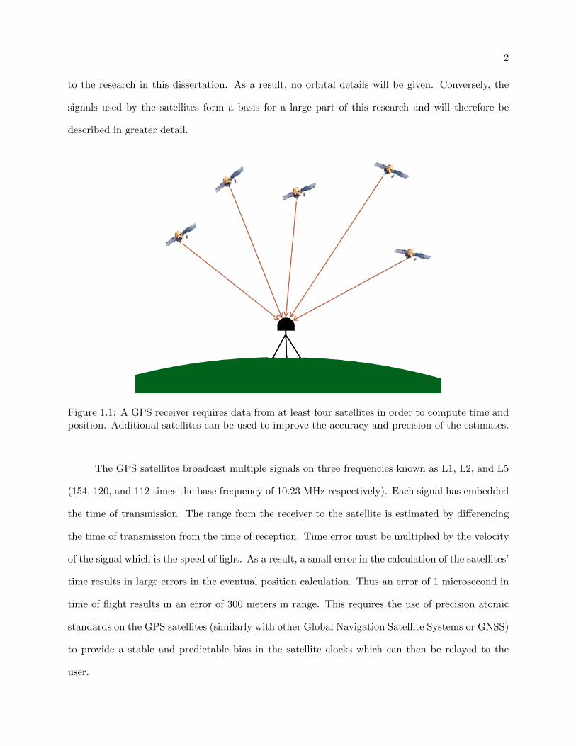
2

to the research in this dissertation. As a result, no orbital details will be given. Conversely, the

signals used by the satellites form a basis for a large part of this research and will therefore be

described in greater detail.

Figure 1.1: A GPS receiver requires data from at least four satellites in order to compute time andposition. Additional satellites can be used to improve the accuracy and precision of the estimates.

The GPS satellites broadcast multiple signals on three frequencies known as L1, L2, and L5

(154, 120, and 112 times the base frequency of 10.23 MHz respectively). Each signal has embedded

the time of transmission. The range from the receiver to the satellite is estimated by differencing

the time of transmission from the time of reception. Time error must be multiplied by the velocity

of the signal which is the speed of light. As a result, a small error in the calculation of the satellites’

time results in large errors in the eventual position calculation. Thus an error of 1 microsecond in

time of flight results in an error of 300 meters in range. This requires the use of precision atomic

standards on the GPS satellites (similarly with other Global Navigation Satellite Systems or GNSS)

to provide a stable and predictable bias in the satellite clocks which can then be relayed to the

user.

3

Besides the error due to time miscalculations, there are other inherent errors in the user-

to-satellite range measurement that must be considered in order to maximize the accuracy and

precision of the position estimate. The range estimate by a receiver to a GPS satellite, known as

pseudorange (ρ), is defined as:

ρ = R+ c(∆tr −∆ts) + I + T +M + ε (1.1)

where R is the true geometric range, ∆tr and ∆ts are the receiver and satellite clock biases with

respect to GPS time, I is the error associated with the signal passing through the ionosphere, T is

the error caused by the signal passing through the troposphere, M is error caused by multipath, and

ε comprises all other noise sources. Each error source is important to consider in the improvement

of GPS positioning.

Besides the time of transmission, the signal meant for coarse acquisition on the L1 frequency

(known as C/A code) has an embedded message containing information about the satellite and

GPS constellation known as the NAV message or broadcast message. This message includes precise

information about the transmitting satellite’s orbit and clock and state of health as well as more

general information about the constellation that allows prediction of which satellites should be

visible. The current GPS broadcast message has errors on the order of 2 meters (RMS) for the

satellite ephemeris (or position) and 5 nanoseconds (about 1.6 meters) for the satellite clock biases

[International GNSS Service, 2009].

An unexpected benefit of GPS is its utility for observation of earth surface conditions. Using

the reflection of the signals from terrain near the GPS antennas many properties of the area

can be inferred. Consequently, various scientific disciplines such as hydrology, oceanography, and

climatology use GPS as a measurement source.

4

1.2 Thesis goals and chapter summary

The purpose of the research detailed in this dissertation is to increase the utility of GPS by

improving primary applications of the constellation and expand the practicality of some secondary

applications. The first three chapters deal primarily with clock applications. The final chapters

address the use of multipath as a measurement source.

Chapter 2 is a general introduction to topics necessary for the work presented in chapters 3

and 4. An introduction to atomic clocks is given and their relative expected performance is discussed

using the Allan deviation. Previous work on the periodic anomaly in GPS clocks is detailed. The

Iridium constellation is also introduced as well as the concept of iGPS and the necessity of modeling

the Iridium clock biases. Prior work in the area of time scales and clock models is shown.

Chapter 3 examines the utility of increasing the number of terms used to represent the

clock bias in the broadcast message. The current accuracy of the broadcast clocks and the size

of the periodic variation in the clock biases are discussed. The accuracy of possible alternative

representations is evaluated and it is shown that the current model is optimal.

The second topic related to timing in this dissertation is the use of a GPS aiding message

broadcast by Iridium Communications System and the possibility of improving the performance of

the primary GPS applications. Chapter 4 develops and discusses a filter to provide an accurate and

stable estimate of the Iridium satellite clocks to make such a message feasible. The measurements

available to the filter are detailed and the performance of the filter is shown to be sufficiently

accurate for the realization of the iGPS system.

Chapters 5 and 6 are an introduction to the work done on expanding secondary applications

involving multipath. The chapters explain the source of multipath and derive the pseudorange

multipath signal which is used as a measurement in chapters 7 and 8. Precedents for using GPS

signals as a measurement of environment are listed. Useful background information is given for

phenology and typical measurements used for vegetation.

The algorithms needed to use pseudorange multipath as a measurement of vegetation are

5

described in chapter 7. This includes the removal of snow and rain corrupted points, the removal

of trends in the underlying receiver noise, and the normalization of the MP1 signal. The processed

signal is shown to correlate well with independent vegetation measurements.

Chapter 8 discusses secondary considerations in the use and preparation of MP1 data as a

vegetation index. These effects include the thermal variation in hardware biases and the effect of

multipath suppression algorithms on MP1.

Chapter 9 concludes the dissertation by discussing the contributions made by this work and

proposing research that could expand upon these points. There are also a number of appendices

following this chapter which clarify or give further background on this work.

Chapter 2

Timing and Clocks

2.1 Precision clocks and the Allan Deviation

As mentioned in the previous chapter, it is important to have a reliable time standard on the

satellite to generate navigation signals in order to minimize positioning errors. Consequently, the

clock must have a predictable drift in bias over long intervals and low noise over short intervals. In

addition, the clock must be able to withstand the harsh environment of space.

There four clock types available for use in space applications where the mission requires

precise time estimates [NIST] are Oven Controlled Crystal Oscillators (OCXO), cesium beams,

rubidium oscillators, and hydrogen masers. All of the clocks generate a signal by controlling a

quartz oscillator. The least expensive and least stable of the clocks is simply an OCXO which

consists of a quartz oscillator enclosed in a chamber (or oven) to maintain a carefully controlled

environment eliminating the noise that typically plagues cheaper clocks. These clocks can have an

accuracy of 10−12 at intervals of 1 second but degrade at longer intervals due to component aging

(in the circuitry or crystal). None of the current GNSS use OCXO clocks due to their instability

at long times, but they are used in the Iridium Communications System as discussed below.

Cesium beam (not to be confused with cesium fountain) and rubidium oscillators work on

similar properties though they differ in resonance frequency [NIST]. The basic idea of both clocks

is that a quartz oscillator is used to generate a microwave beam at a frequency based on the

frequency of the quartz oscillator and the voltage being applied. The beam interacts with a gas

of the rubidium or cesium particles contained in a chamber. A portion of the particles are excited

7

based on the frequency of the beam. A measurement of the number of excited particles indicates

the offset in the frequency from the nominal, which is fed back into the system in order to adjust

the voltage being applied to the crystal. Rubidium clocks are generally smaller and cheaper while

cesium clocks have better stability over long intervals. Advances in rubidium clocks have, however,

made them more accurate in space applications resulting in the use of rubidium clocks in nearly

all of the current GPS satellites [USNO].

The final clock type, just beginning to see use in space applications, is the hydrogen maser.

Currently the best example of this is the GIOVE-B satellite [Waller et al., 2008] which is being

tested for the Galileo system. At intervals of a few days or less, hydrogen maser standards are

generally at least an order of magnitude better than any other frequency standard flown in space

[Waller et al., 2008].

There are several different ways to characterize the stability of, or noise in, a clock. Unlike

the standard variance (the square of the standard deviation) that is used to characterize most

other measurement types, accurately describing clock noise requires more than a single number.

The existence of several noise types in clock measurements results in different variance estimates

depending on the sampling interval used. Plotting clock variance versus sampling interval exposes

the different noise types that are present in the clock measurements (Figure 2.1). The most com-

monly used description of clock stability is known as the Allan deviation [Riley, 2008] (which is

the square-root of the Allan variance). For most applications either the Allan or modified Allan

deviation is sufficient to model the clock stability. The modified Allan deviation, which is used

throughout this dissertation, is defined in the equation below with N bias measurements, x, over m

time steps, τ . For additional detail on the Allan and modified Allan deviations refer to Appendix

A.

σy(τ) =

√√√√√ 1

2m2(N − 3m+ 1)τ2

N−3m+1∑k=1

k+m−1∑j=k

xj+2m − 2xj+m + xj

2

(2.1)

The four types of precision clocks described above can be expected to fall within a certain

8

Figure 2.1: Example modified Allan deviation of a clock with noise types noted as well as the slopethat results from that noise type.

range of deviations (see figure 2.2). The type of clock (i.e. rubidium) will determine its approximate

stability. However, manufacturing quality and environment are also factors in determining the exact

stability of a clock. As newer manufacturing techniques are created, the stability of the clocks can

improve beyond the expected bounds as evidenced by the rubidium clocks being used on the new

GPS block II-F satellites, which exhibit a stability about one order of magnitude greater than

previous rubidium standards [Montenbruck et al., 2011; Vannicola et al., 2010].

2.2 Periodic variation in GPS clocks

Precision clocks are typically used in controlled environments which limits external influences

such as temperature and radiation on the system. Precision clocks used in space-based applications,

on the other hand, are susceptible to such factors. As a result, periodic variations exist in the

GPS satellite clocks as described by several papers. The most comprehensive paper detailing

9

Figure 2.2: Typical Allan deviations experienced by quartz(blue), rubidium(green), cesiumbeam(red), and hydrogen maser clocks(yellow). Typical values based on figures in [Coates, 2014;Vig, 1992; Allan et al., 1997].

these periodic variations was done by Senior et al. [2008] but their existence was recognized 20

years earlier by Swift and Hermann [1988]. Periodic variations have also been shown by Bahder

[1998], Montenbruck et al. [2011], and Vannicola et al. [2010]. These papers demonstrated that

there is a periodic component to the GPS clock error at intervals of once and twice per satellite

orbit revolution (as well as some minor lower harmonics) and that these variations can introduce

significant clock prediction error if the clocks of the GPS satellites are modeled linearly. The effect

is most pronounced in the older block IIA satellites. The variation is a result of thermal variations

which has been proven by clock variability due to eclipses.

Heo et al. [2010] have suggested an approach to mitigate the periodic variations by prediction

using a dynamic system from past observations based on a model of linear and periodic terms. The

method was shown to improve near real-time clock estimates from the International GNSS Service

10

(IGS) as well as the GPS broadcast message when the estimates are used to predict for intervals

greater than 12 hours. The IGS is an international collaboration that pools resources from hundreds

of permanent GPS stations (as well as other current and future GNSS systems) to provide both raw

measurement data and products that improve the accuracy of GPS positioning estimates (such as

improved orbit and clock estimates). The improvement is most pronounced in GPS satellites using

cesium clocks. For predictions less than 12 hours little improvement is seen over the traditional

methods.

2.3 iGPS and the Iridium constellation

An accurate estimate of clock bias is also important for GPS aiding systems. One such

system, called High Integrity GPS or iGPS, was considered by the Office of Naval Research to

improve the position, navigation, and timing performance for military GPS users by integrating

the communications capability of the satellite network from Iridium Satellite LLC, hereafter referred

to as Iridium. The Iridium constellation consists of 66 satellites in low Earth orbit. These satellites

communicate with each other and the Iridium ground stations, or earth terminals, as well as users.

With its network of satellites supplying coverage of the entire planet, Iridium provides global voice

and data telecommunication services to both military and commercial customers with equipment

and services targeting numerous markets such as maritime, aviation, defense/government, machine-

to-machine communications, disaster response, and exploration/adventure ([Schuss et al., 1999;

Foosa et al., 1998]).

The iGPS concept uses the Iridium communications capability to precisely transfer GPS time

to properly equipped users in challenging environments such as natural and urban canyons, heavily

wooded areas, and in the presence of intentional or unintentional interference. By establishing a

robust means to provide this time to within 0.5 µs, the system would facilitate the acquisition of

GPS and accelerate the time to first fix for properly authorized users in degraded environments.

More information on using Iridium to augment GPS can be found in Joerger et al. [2010] and

[Joerger et al., 2009].

11

Figure 2.3 shows the general architecture of the iGPS system, which consists of reference

stations and Iridium earth terminals that gather information from passing satellites and then relay

that data to an operations center. To effectively utilize the Iridium constellation for ranging and

augmentation of GPS, the position of the satellites must be known and the behavior of the satellite

clocks must be estimated accurately and characterized with respect to GPS time. Each of the

reference stations has a Rubidium clock calibrated to GPS time using an independent single-

frequency GPS receiver. Using the data collected from all the reference stations, the operations

center determines the ephemeris and clock biases of the Iridium satellite constellation. The Iridium-

augmented GPS reference stations are separate from the Iridium stations that are used for the

standard constellation control and maintenance.

Figure 2.3: iGPS elements and signals. iGPS uses several reference stations that receive and processsignals from both the GPS and Iridium satellites. Each reference station uses GPS information todetermine the bias in its reference clock. The central estimator at the operations center uses theIridium downlink and crosslink signals to determine the Iridium satellite clock biases.

12

The Iridium satellites are in six orbital planes located in a low-Earth orbit altitude of approx-

imately 780 km with a high inclination of ∼86◦. This leads to relatively short contact times with

the ground, for 10 min or less, but higher received power signals than GPS. Each of the satellites

is assigned a satellite vehicle (SV) number. The SV numbers are used to identify results shown in

later sections.

The Iridium satellites use oven-controlled crystal oscillators onboard to generate the commu-

nications signals and maintain system time. Over short time intervals, these clocks are very stable,

but over time spans larger than 100 s, the clocks exhibit greater noise than the atomic clocks used

by GPS satellites. The Iridium satellite clocks generally exhibit a flicker noise floor below 10−11

s/s from intervals of 0.1 to a few hundred seconds. At an interval of about 1,000 s and onward, the

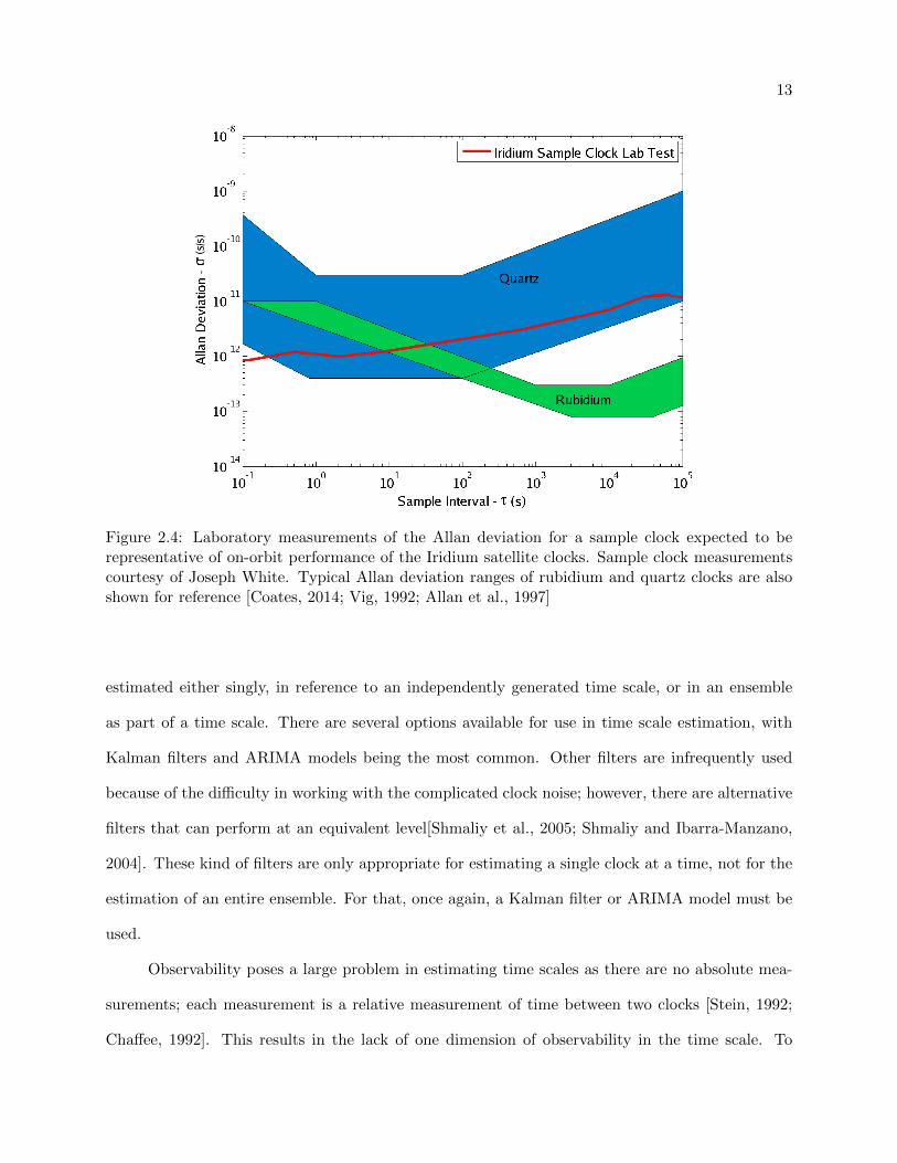
satellite clocks exhibit random walk behavior, still below 10−11 s/s (Figure 2.4). Although this is

the nominal behavior of the clocks, some do exhibit less stable behavior. Iridium issues commanded

bias and frequency adjustments to each of the satellites at least twice per day to keep the clocks

synchronized. Satellites with higher instabilities are updated more frequently, with no limit set by

Iridium on how many times per day any satellite’s clock can be adjusted.

2.4 Clock Modeling and Time Scales

The foundation of the iGPS clock estimator is the extensive time scale research that has been

done. When estimating clocks for the purpose of a time scale, they are generally modeled as perfect

integrators. That is, the bias is the integral of the frequency, and the frequency is the integral of the

frequency aging or frequency drift. This is covered in detail by Stein in [Stein, 1992, 2003]. White

noise is added to the bias, frequency, and frequency drift but the fact that the bias and frequency

are integrating lower terms results in colored noise associated with the bias and frequency. This

leads to complicated noise models required to adequately describe the noise process in the clock

system[Jones and Tryon, 1987].

A clock ensemble consists of a group of clocks that are used together to estimate a single time.

The time resulting from the ensemble is known as a time scale [Stein, 1992]. Clocks are generally

13

Figure 2.4: Laboratory measurements of the Allan deviation for a sample clock expected to berepresentative of on-orbit performance of the Iridium satellite clocks. Sample clock measurementscourtesy of Joseph White. Typical Allan deviation ranges of rubidium and quartz clocks are alsoshown for reference [Coates, 2014; Vig, 1992; Allan et al., 1997]

estimated either singly, in reference to an independently generated time scale, or in an ensemble

as part of a time scale. There are several options available for use in time scale estimation, with

Kalman filters and ARIMA models being the most common. Other filters are infrequently used

because of the difficulty in working with the complicated clock noise; however, there are alternative

filters that can perform at an equivalent level[Shmaliy et al., 2005; Shmaliy and Ibarra-Manzano,

2004]. These kind of filters are only appropriate for estimating a single clock at a time, not for the

estimation of an entire ensemble. For that, once again, a Kalman filter or ARIMA model must be

used.

Observability poses a large problem in estimating time scales as there are no absolute mea-

surements; each measurement is a relative measurement of time between two clocks [Stein, 1992;

Chaffee, 1992]. This results in the lack of one dimension of observability in the time scale. To

14

account for this the “basic time scale equation” is added to the list of relative measurements be-

tween clocks [Stein, 1992, 2003; Greenhall, 2001]. The “basic time scale equation” is simply the

assumption that the sum of the difference between predicted and measured clock bias across all

clocks is zero or, equivalently, that the sum of the noise in the bias state (adjusted by clock weights)

is zero. A similar equation can also be used with the frequency and frequency drift.

The typical Kalman filter and ARIMA model for time scales perform at a comparable level,

at steady-state. The Kalman filter, however, has some properties which recommend it over the

ARIMA model, such as: ability to use unequally spaced data, better warm-up performance, and

better adaptability when the filter is concurrently determining noise parameters (eg. Stein and

Evans [1990]). A good reference for clock estimation using ARIMA models is provided by Barnes

[1988] and Stein and Evans [1990].

There are many papers covering the estimation of clocks using Kalman filters. Much of the

original work was done by Allan and Barnes [1982] and Jones and Tryon [1987]. Stein has does an

excellent job developing and summarizing the work of time scales using Kalman filters in several

papers ([Stein, 1992, 2003; Stein and Evans, 1990; Stein and Filler, 1988; Stein, 1989]) and extensive

work has also been done by Greenhall in several publications ([Greenhall, 2001; Davis et al., 2005;

Greenhall, 2006]).

2.5 Contributions of this work

Although the presence of the periodic variation in the GPS clocks is well known and docu-

mented, it is unknown if this causes measurable error in the linear model used by the GPS broadcast

message for propagating clock bias. As a majority of GPS receivers use the GPS broadcast message,

understanding and, if possible, correcting these errors is important. However, the GPS broadcast

message is, by necessity, limited in the amount of information that can be conveyed so all bits must

be used as optimally as possible. Chapter 3 discusses the possibility of any possible improvements

and whether the improvements would merit inclusion in the NAV (or new CNAV) message.

Chapter 4 describes the design of a clock estimation algorithm for the Iridium constellation

15

satellite clocks. The generated estimates were intended for use with the iGPS system to provide

users with an estimate of the clock bias for each of the satellite clocks. Many of the aspects of this

project differ from the time scale estimation discussed in the prior work section. Unlike time scales,

there is no issue with observability as the goal is not to determine time from an ensemble of clocks

but instead to determine the bias of the satellite clocks with respect to GPS time. This is done

using measurements between the satellites, which give an indication of the relative biases of the

satellite clocks, and measurements involving the ground stations, that measure the bias between the

satellite and ground clock. As the ground clocks are all independently estimated against the GPS

constellation, the ground measurements are not ambiguous and give an estimate of the satellite

clock relative to GPS time. The inter-satellite measurements allow the algorithm to continue to

update all the satellite clocks despite the small fraction that are within range of a ground station

at any one time.

The noise and bias in the measurements require designing a system that is very robust in

the presence of noisy data, unlike most clock estimation problems where the measurement noise

is relatively low. It is also necessary for the algorithm controlling the iGPS clock estimates to

be able to handle frequent unplanned clock adjustments in both frequency and time. Most such

clock estimators are running on very stable atomic clocks and thus the clocks are infrequently

adjusted; the Iridium clocks are simple OCXO standards and are updated at least twice per day.

The algorithm is conditioned such that adjusts are quickly recognized and incorporated while

anomalous measurements do not cause the filter to go unstable or give large errors.

Chapter 3

The improvement of the GPS broadcast clock correction by using periodic

terms

Although the presence of the periodic variation in the GPS clocks is well known and docu-

mented, it is unknown if this causes measurable error in the linear model used by the GPS broadcast

message for propagating clock bias. As a majority of GPS receivers use the GPS broadcast message,

understanding and, if possible, correcting these errors is important. However, the GPS broadcast

message is, by necessity, limited in the amount of information that can be conveyed so all bits must

be used as optimally as possible. This chapter discusses the possibility of any possible improvements

and whether the improvements would merit inclusion in the NAV (or new CNAV) message.

3.1 Accuracy of the GPS Satellite Clocks

The GPS system currently uses rubidium atomic clocks (with some legacy cesium standards)

for the essential task of maintaining the on-board satellite time with respect to the GPS time scale.

These clocks have steadily improved stability with each new generation of satellites. The newest

generation, Block IIF, have shown a remarkable reduction in clock noise over previous generations

[Vannicola et al., 2010].

The GPS satellites broadcast information to users about the position and state of the satellite

in a data stream known as the broadcast message. Three of the variables conveyed in the message

(known as the a0, a1, and a2 terms) represent the clock bias, frequency offset, and frequency drift.

The set of terms being broadcast is changed every 2 hours. A new set of two hour sets is estimated

17

and uploaded to the satellites at intervals of typically about 20 hours.

Although the GPS broadcast model makes available three terms for the representation of the

clock bias, only the first two terms (bias and frequency offset) are ever used. The final term (fre-

quency drift) is always set to zero. This is a result of the resolution selected for the frequency drift

component the design of the broadcast message. The message allocates 8 bits for a 2s complement

representation of the frequency drift. The number is then scaled by 2−55 [Interface Specification,

Revision G], resulting in a resolution of 3e-17 sec/sec2. Typical frequency drift values for the GPS

satellite clocks range from 1e-18 to 1e-17, too low to be accurately represented. This decreases

the accuracy of the estimates provided by the broadcast message as only a linear representation is

actually possible.

The current accuracy of the GPS broadcast clock message is about 5 nanoseconds or 1.5

meters whereas the error in the orbits provided by the broadcast message is only 1 meter [Inter-

national GNSS Service]. The presence of periodic variations in the GPS satellite clocks is a well

known phenomenon as shown by sources referenced in the introductory chapter. The goal of this

project is to determine if there is a possible improvement in the GPS broadcast clock message by

adding additional broadcast variables, which would ultimately improve positioning.

The analysis of the accuracy of the GPS satellite clocks was done using data from the Inter-

national GNSS Service (IGS) [International GNSS Service]. The best IGS clock products have an

accuracy of 75 ps RMS and a precision of 25 ps. The clock bias products used in this paper are

provided at an interval of 30 seconds. The other data necessary for the processing shown are also

available from the IGS (such as the broadcast messages for the dates analyzed).

3.2 Periodic Portion of the GPS Clock Bias

The periodic portion of the GPS satellite clocks was determined for several data sets with

consistent results. Forty days of data starting on January 10, 2012 are used for the results shown

in this chapter. The first ten days being used to initialize the model. All PRNs were used except

3, 24, and 26 as PRN 24 was unassigned at the time and PRNs 3 and 26 were marked as unusable

18

during a portion of the data set.

Two main frequencies dominate the periodic portion of the GPS satellite clock bias. These

occur at roughly once and twice per orbital revolution of the GPS satellites with mean magnitudes

from all satellite clocks at the two main frequencies being 0.72 and 0.22 nanoseconds respectively.

Although some minor harmonics do exist, they have magnitudes at least one order smaller and are

therefore irrelevant to this analysis [Senior et al., 2008].

The magnitude of the bias at the two main frequencies varies widely by satellite. The mag-

nitudes were calculated using a fast fourier transform analysis on the data set after detrending the

clock biases with a quadratic. Though the once per orbit signal is typically stronger, there are

some satellites with relatively equal magnitudes for the two frequencies or, very rarely, a stronger

signal at the twice per orbit frequency. Figures 3.1 through 3.4 show the amplitude of the two main

periodic signals in each of the clock biases.

The results in figures 3.1 through 3.4 are separated by satellite manufacturing groups (referred

to as generations) denoted as Block IIA, IIR, IIR-M, or IIF. Each of the generations used different

clocks resulting in different clock stabilities. It can be seen that the block IIA satellites (Fig. 3.1)

have much larger periodic components than the newer generation satellites. However, even the

newest block IIF satellites (Fig. 3.4) show evidence of small periodic components. The cesium

clocks being used on some of the block IIA have the largest periodic components with three out of

four having once per orbit amplitudes above 2 nanoseconds.

The Block IIR, IIR-M, and IIF satellites show a relatively consistent mean value (though it

is difficult to generalize for Block IIF from such a small sample set), while the Block IIA satellites

exhibit much larger periodic variations (as previously mentioned). Over all generations, the periodic

effect has a magnitude of about 12% of the size of the total clock bias uncertainty. Looking at just

the newer satellite generations, the mean magnitude is only about 4% of the uncertainty.

To model the satellite clock bias, a signal is defined consisting of a quadratic and 2 periodic

19

Figure 3.1: Amplitudes of the once per orbit and twice per orbit signals in the clock biases of theBlock IIA GPS satellites. For the specified dates there were 8 Block IIA satellites in operation. Theclock type is indicated next to the PRN (Mx means the clock type changed during the specifiedperiod). The mean magnitude of the biases at the two dominant frequencies were 2.14 and 0.49nanoseconds. The red dashed line indicates the maximum y value in the plots for the other satellitegenerations (for comparison purposes).

elements. The clock bias signal sb(t) can be written as:

sb(t) = q0 + q1t+ q2t2 +A1 sin(ω1t+ φ1) +A2 sin(ω2t+ φ2) (3.1)

where qj represents the jth quadratic term and Ai, ωi, and φi are, respectively, the amplitude,

the angular frequency, and the phase of the ith periodic element. Using the summation of angles

identity for trigonometric functions, sb(t) can be written as:

sb(t) = q0 + q1t+ q2t2 +A1 cos(φ1) sin(ω1t) +A1 sin(φ1) cos(ω1t) + ...

A2 cos(φ2) sin(ω2t) +A2 sin(φ2) cos(ω2t) (3.2)

This model will be used in the following sections to analyze the clock bias.

20

Figure 3.2: Amplitudes of the once per orbit and twice per orbit signals in the clock biases of theBlock IIR GPS satellites. For the specified dates there were 12 Block IIR satellites in operation.All were using rubidium clocks. The mean magnitude of the biases at the two dominant frequencieswere 0.19 and 0.10 nanoseconds.

Figure 3.3: Amplitudes of the once per orbit and twice per orbit signals in the clock biases ofthe Block IIR-M GPS satellites. For the specified dates there were 7 Block IIR-M satellites inoperation. The clock type is indicated next to the PRN (MX means mixed or both rubidium andcesium). The mean magnitude of the biases at the two dominant frequencies were 0.20 and 0.15nanoseconds.

21

Figure 3.4: Amplitudes of the once per orbit and twice per orbit signals in the clock biases of theBlock IIF GPS satellites. For the specified dates there were 2 Block IIF satellites in operation. AllBlock IIF satellites will be using rubidium clocks. The mean magnitude of the biases at the twodominant frequencies were 0.15 and 0.14 nanoseconds.

3.3 GPS Clock Bias Representations

In order to determine possible improvement in the GPS broadcast clock uncertainty through

the addition of extra clock variables in the broadcast message, the efficiency of various representa-

tions for the GPS clock bias was studied. Results from the following likely models are shown in this

paper: linear, quadratic, linear plus periodic terms, and quadratic plus periodic terms. Multiple

time steps are considered for each of the models as well. The linear two-hour model is the baseline

for comparison as it is the current model used by the broadcast message. The periodic sets at time

intervals of 6 hours or less have observability issues when paired with a quadratic set so the high

rate sets were paired with simple linear fits only.

Typically, fitting a model involving two periodic terms of unknown frequency and a quadratic

to a signal would be a complicated non-linear process. However, the frequencies of the periodic

signals have been detailed in [Senior et al., 2008] and shown to have a variation in their period

22

of less than 30 seconds. Using the assumed frequencies, the unknowns in equation (3.2) can be

reduced to the four amplitudes Ai cos(φi) and Ai sin(φi) for i = 1, 2. The resulting system avoids

the difficulties of non-linear estimation which makes it an excellent candidate for least-squares

estimation. Appendix B shows the process and feasibility of least-squares estimation for this system.

The final equations are shown below in (3.3) where X is the system state and H shows the response

of the system to a clock bias measurement.

X =

A1 cos(φ1)

A1 sin(φ1)

A2 cos(φ2)

A2 sin(φ2)

q0

q1

q2

(3.3a)

H =

sin(ω1t1) cos(ω1t1) sin(ω2t1) cos(ω2t1) 1 t1

12 t

21

......

......

......

...

sin(ω1tn) cos(ω1tn) sin(ω2tn) cos(ω2tn) 1 tn12 t

2n

(3.3b)

Using (3.3), the best possible fit of the clock bias was made for each parameter set. Figure

3.5 shows the fit for PRN 16 (a rubidium clock) over one days worth of data using five of the

most accurate parameter sets as well as the current 2 hour linear model. The clock data have been

detrended so that the smaller variations can be seen. The error of each parameter set with respect

to the final clock solutions is shown in figure 3.6 with the RMS values of the error indicated in

the legend. The various representations show little difference with the error only varying by 10%

relative to the error in the linear set.

Similar calculations were made for all valid PRNs for each day over the interval of the data

set. The mean of the RMS from each of these daily models was computed. Figures 3.7 through

3.10 show the values for each parameter set separated by satellite generation and 3.11 and 3.12

23

summarize the results for the entire constellation. The most optimal representation for the GPS

satellite clock biases was found to be one that allowed modeling of both periodic signals as well as

a linear parameter set that was updated at intervals of two hours. The quadratic set updated at

2 hour intervals showed similar accuracies to set update at 4 hours that modeled both periodic as

well as a line. A set updated at 2 hour intervals and consisting of one periodic signal (the dominant

once-per-orbit) and a line had accuracies midway between the 2 hour and 4 hour sets that used both

periodic signals. The model equivalent to the current format, a line updated at 2 hour intervals,

has errors generally between 150 and 200 ps for satellites using rubidium clocks. The best model

improves upon that by 20 to 150 ps for these satellites. The GPS satellites that are using the older

cesium clocks have typical errors between 500 and 700 ps with the improved model reducing that

to 300 ps. The new block IIF satellites have errors with the 2 hour linear model on the order of 30

ps. This is reduced by about half for the 2 hour linear plus periodic model.

Although the periodic sets outperformed the simpler quadratic sets, this was mostly due to

the increased number of parameters that the least squares system could fit. A linear model updated

on a 2 hour basis performed very closely to a linear plus periodic model updated on a 6 hour basis.

Both of these models require 6 parameters every 6 hours. Similarly, figure 3.13 shows a comparison

of two of the periodic based models with a 1 hour linear and 1 hour quadratic set. The models

are matched very closely based upon the number of parameters available to fit with only a small

improvement shown occasionally in the models using the periodic sets.

24

Figure 3.5: Comparison of the detrended final clock bias for PRN 16 with the ability of the variousmodels to fit the bias. The data are from January 17th, 2012. The different models performed ina comparable manner.

25

Figure 3.6: Difference between the model and the final clock bias for PRN 16 over one day (January17th, 2012). The RMS of the error is indicated in the legend for each model. The model that bestfits the actual data was the model combining two periodic sets with a line every 2 hours. Thedifference in error, however, was only about 10% from the simple two hour linear model currentlybeing used.

26

Figure 3.7: The mean of the daily RMS of the error between the final clock bias and each of theparameter sets used to model it for all of the Block IIA GPS satellites. The y limit for the othersatellite generations is marked as a red, dashed line. The clock type is marked except for satellitesthat are not using a rubidium clock (Mx means mixed or both rubidium and cesium).

Figure 3.8: The mean of the daily RMS of the error between the final clock bias and each of theparameter sets used to model it for all of the Block IIR GPS satellites. All the satellites were usingrubidium clocks.

27

Figure 3.9: The mean of the daily RMS of the error between the final clock bias and each of theparameter sets used to model it for all of the Block IIR-M GPS satellites. The clock type is markedexcept for satellites that are not using a rubidium clock (Mx means mixed or both rubidium andcesium).

Figure 3.10: The mean of the daily RMS of the error between the final clock bias and each of theparameter sets used to model it for all of the Block IIF GPS satellites. All the satellites were usingrubidium clocks.

28

Figure 3.11: The mean of the daily RMS of the error between the final clock bias and each of theparameter sets used to model it for all of the GPS satellites. The different satellite generations areseparated by red, dashed lines.

Figure 3.12: The mean of the daily RMS of the error between the final clock bias and each of theparameter sets used to model it for all of the GPS satellites. The different satellite generations areseparated by red, dashed lines. The y-axis has been reduced from figure 3.11 to show the differencesbetween the models for the more stable satellite clocks.

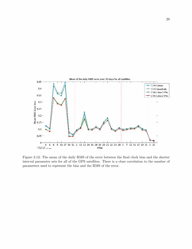
29

Figure 3.13: The mean of the daily RMS of the error between the final clock bias and the shorterinterval parameter sets for all of the GPS satellites. There is a close correlation to the number ofparameters used to represent the bias and the RMS of the error.

30

3.4 Conclusions

Relatively small gains are achieved by using a more complicated representation of the GPS

satellite clocks in the broadcast message. Most of the gains over the current 2 hour linear model

were less than 100 ps with only the most unstable clocks showing improvements greater than 100

ps. These clocks, however, are the ones that are being transitioned out as newer satellites are

launched. For example, the satellite which was broadcasting PRN 27 (which used a cesium clock)

was decommisioned on October 6, 2012 and PRN 27 is now broadcast by a Block IIF satellite.

Even the errors seen above in the more unstable clocks is minuscule in comparison to the 5 ns

uncertainty in the GPS broadcast clocks.

In addition, the deficiency in the clock terms of the broadcast message has been corrected

in the new CNAV message available on GPS L2C signals. The frequency drift term present in the

transmitted CNAV clock corrections consists of 10 bits scaled by 2−60. This allows for a resolution

of 8.67e-19 sec/sec2 and a maximum value of 4.44e-16 sec/sec2. This is more consistent with values

observed in the GPS satellite clocks and allows for a true quadratic representation of the clock bias.

Despite this, even the correction of the frequency drift terms is unnecessary as the linear model at

2 hour intervals is able to represent the clock biases at well below the uncertainty in the estimates.

Although the inclusion of periodic terms is not useful for the broadcast message, it is an

important part of the estimation of the clocks as part of the GPS time scale. This is discussed in

Appendix C.

Chapter 4

Estimates of iGPS satellite clocks

This work was previously published as Pratt et al. [2012].

4.1 Introduction

The Office of Naval Research sponsored High Integrity GPS (iGPS) Technology Concept

Demonstration Program is designed to improve the position, navigation, and timing performance

for military GPS users by integrating the communications capability of the satellite network from

Iridium Satellite LLC, hereafter referred to as Iridium. The Iridium constellation consists of 66

satellites. These satellites communicate with each other and the Iridium ground stations, or earth

terminals, as well as users. With its network of satellites supplying coverage of the entire planet,

Iridium provides global voice and data telecommunication services to both military and com-

mercial customers with equipment and services targeting numerous markets such as maritime,

aviation, defense/government, machine-to-machine communications, disaster response, and explo-

ration/adventure ([Schuss et al., 1999; Foosa et al., 1998]).

The iGPS concept uses the Iridium communications capability to precisely transfer GPS time

to properly equipped users in challenging environments such as natural and urban canyons, heavily

wooded areas, and in the presence of intentional or unintentional interference. By establishing a

robust means to provide this time to within 0.5 ls, the system will facilitate the acquisition of GPS

and accelerate the time to first fix for properly authorized users in degraded environments. More

information on using Iridium to augment GPS can be found in Joerger et al. [2010] and [Joerger

32

et al., 2009].

The Iridium satellites are in six orbital planes located in a low-Earth orbit altitude of ∼780

km with a high inclination of ∼86◦. This leads to relatively short contact times with the ground,

for 10 min or less, but higher received power signals than GPS. Each of the satellites is assigned a

satellite vehicle (SV) number. The SV numbers are used to identify results shown in later sections.

The Iridium satellites use oven-controlled crystal oscillators onboard to generate the commu-

nications signals and maintain system time. Over short time intervals, these clocks are very stable,

but over time spans larger than 100 s, the bias and drift of these clocks are less stable than the

atomic clocks used by GPS satellites. The Iridium satellite clocks generally exhibit a flicker noise

floor below 10−11 s/s from intervals of 0.1 to a few hundred seconds. At an interval of about 1,000

s and onward, the satellite clocks exhibit random walk behavior, still below 10−11 s/s (Fig. 4.1).

Although this is the nominal behavior of the clocks, some do exhibit less stable behavior. Iridium

issues commanded bias and frequency adjustments to each of the satellites at least twice per day

to keep the clocks synchronized. Satellites with higher instabilities are updated more frequently,

with no limit set by Iridium on how many times per day any satellite can be adjusted.

Figure 4.2 shows the general architecture of the iGPS system, which consists of reference

stations and Iridium earth terminals that gather information from passing satellites and then relay

that data to an operations center. To effectively utilize the Iridium constellation for ranging and

augmentation of GPS, the position of the satellites must be known and the behavior of the satellite

clocks must be estimated accurately and characterized with respect to GPS time. Each of the

reference stations has a Rubidium clock calibrated to GPS time using an independent single-

frequency L1 GPS receiver. Using the data collected from all the reference stations, the operations

center determines the ephemeris and clock biases of the Iridium satellite constellation. The Iridium-

augmented GPS reference stations are separate from the Iridium stations that are used for the

standard constellation control and maintenance.

We describe an approach to globally estimate the bias for each Iridium satellite clock using

inter-satellite and satellite-to-ground ranging signals. The basic methodology is first presented,

33

Figure 4.1: Laboratory measurements of the Allan deviation for a sample clock expected to berepresentative of on-orbit performance of the Iridium satellite clocks. Sample clock measurementscourtesy of Joseph White. Typical Allan deviation ranges of rubidium and quartz clocks are alsoshown for reference [Coates, 2014; Vig, 1992; Allan et al., 1997]

followed by some example results.

4.2 Measurement Models and Characteristics

There are two measurement types available to the Iridium global satellite clock estimator.

The first type, which is similar to GPS pseudorange, is an L-band downlink ranging measurement

between an Iridium satellite and a reference station. The second measurement type is a K-band

ranging signal between neighboring Iridium satellites, referred to as a crosslink measurement. The

basic structure of each is developed below.

In order to use the downlinks or crosslinks to determine clock bias, the locations of the Iridium

satellites must be well known. The locations of the Iridium satellites used for this research were

calculated from an ephemeris set generated by the Iridium operations group. These are currently

34

Figure 4.2: iGPS elements and signals. iGPS uses several reference stations that receive and processsignals from both the GPS and Iridium satellites. Each reference station uses GPS information todetermine the bias in its reference clock. The central estimator at the operations center uses theIridium downlink and crosslink signals to determine the Iridium satellite clock biases.

accurate to better than 20 m. Also necessary for the use of the downlink measurements are the

locations of the reference stations. These have been determined using GPS precise point positioning

with an expected accuracy of better than 10 cm.

The currently implemented satellite to reference station downlink signal provides an unam-

biguous measurement of the satellite clock relative to the reference station clock with a noise level

of about 600 ns. The bias and drift of the reference station clock are solved for separately using

GPS signals. The uncertainty of these estimates is typically between 10 and 20 ns, much smaller

than the Iridium satellite clock errors and measurement noise present in the typical downlink. The

timing error in the downlink signal therefore is chiefly a result of the Iridium satellite clock bias

and the measurement processes involved in the downlink itself, as seen below. The downlink range

35

measurement, D, can be modeled as:

D =R

c+ tof +Bref −Bsat + εref − εsat + γ + η (4.1)

where R is the geometric range, tof is the time-of-flight correction, Bref is the reference

station clock bias, Bsat is the satellite clock bias, εref is the reference station receiver hardware

bias, εsat is the satellite transmitter hardware bias, γ includes the ionospheric and tropospheric

delays, and η represents all other error sources.

Using the satellite and reference station position information, the geometric range and time-

of-flight correction are removed from the downlink signal. The reference station bias, as calculated

via GPS, is also removed. Because of the relatively coarse ranging requirements, the tropospheric

delay is simply modeled as a site-specific constant divided by the sine of the elevation angle of the

satellite relative to the reference station. This should remove about 75% of the associated error

leaving residual troposphere errors of less than 2 ns. The ionosphere and remaining troposphere

error, residual ephemeris error, multipath, and tracking noise are combined in the variable η′ and

are expected to be less than 50 ns. The downlink residual model is then given by:

δD = −Bsat + εref − εsat + η′ (4.2)

A downlink pass lasts between 3 and 10 min with a data rate of one measurement per second.

Figure 4.3 shows the residuals for a typical pass. At intervals of less than 10 min, the Iridium

clocks have an expected time deviation ([Riley, 2008]) of less than 1.1 ns. Thus, for the purpose of

determining the Iridium satellite clock biases to better than 0.5 µs, the high-rate downlink range

measurements can be reduced to a single bias and drift value for the pass, by simply applying

a linear least squares fit to the downlink residuals. The bias value estimated at the midpoint of

the pass is then input as a measurement to the global satellite clock estimator. The measurement

uncertainty is determined from the covariance of the least squares fit.

The downlink example in figure 4.3 shows a pass of about 7.5 min. The original downlink

36

observations have 1σ noise of 600 ns. For typical downlink passes, the resulting midpoint bias

formal uncertainty is reduced to between 25 and 45 ns, depending on the length of the downlink

pass. As a result of hardware biases and other unmodeled systematic errors, the actual error in

the downlink measurements is estimated to be about 100 ns. The results shown are typical of the

downlink preprocessing.

Figure 4.3: Preprocessing of downlink measurements to create downlink observable. The individualdownlink measurement residuals received by the reference stations currently have a 0.6 µs level ofnoise. Over short time intervals, the clock exhibits mostly linear behavior. By fitting a line andusing a single point from the midpoint as a representative aggregate observable, the measurementnoise input to the filter and computational load are reduced.

The crosslink measurement set includes an unambiguous but noisy range measurement known

as a variable receive offset (VRO) measurement, and a precise but ambiguous range measurement

known as a unique word phase (UWP) measurement. As the current design favors simplicity and

accuracy over precision, only the VRO measurements are currently being used. Each satellite has

the potential to measure four crosslink ranges with satellites in front and behind it in the same

orbital plane and with one satellite in each neighboring orbital plane. The specific cross-plane

crosslinks vary depending on whether the satellite is ascending or descending in its orbit. The

37

satellites in the first and sixth plane, which are moving in opposite directions, do not communicate

with each other.

The in-plane crosslink range measurements have lower noise than the cross-plane crosslinks,

but both are useful for connecting clock measurements across the satellite network. In general, the

precision of the in-plane crosslink measurements is on the order of 2 ns. The overall accuracy of the

measurements though is closer to 20 ns, again due to uncalibrated biases and unmodeled systematic

effects (Fig. 4.4). The cross-plane crosslink observations have errors that are two to three times

larger, depending on the satellites. Despite this, the cross-plane crosslinks are very important for

keeping all satellites clock biases observable when an orbital plane lacks downlink measurements.

It should be noted that cross-plane measurements are not made by the satellites when they are

near the poles of the Earth, because of the potentially short ranges between neighboring satellites

in the region where the orbital planes cross. The accuracy of the cross-plane measurements is also

better near the equator.

Figure 4.4: Comparison of the noise in the in-plane crosslink VRO measurement, which is beingused in the filter, and the more precise UWP measurement. There are systematic errors in theVRO measurement, especially when the satellite is in high-latitude regions.

38

The crosslink range, R, between the two satellites is measured by each of the satellites involved

in the link. The one-way link from satellite A to satellite B is referred to as χAB. Differencing two

one-way measurements for the same link removes the geometrical range and common error sources

including the minimal atmospheric effects present at an altitude of 780 km. The two-way crosslink

measurement is referred to as XAB.

χAB =RABc

+BA −BB + εrecA − εtrB + η (4.3a)

χBA =RBAc

+BB −BA + εrecB − εtrA + η (4.3b)

XAB = χAB − χBA

= 2(BA −BB) + εrecA − εtrB − εrecB + εtrA + η (4.4)

The ranges from A to B, RAB, and from B to A, RBA, include the time-of-flight difference

between the two ranges. Time-of-flight would not be removed through differencing, because the

value is different for each of the two one-way links. Therefore, a time-of-flight-adjusted range is

removed from each one-way link before differencing. The range adjustment is calculated based on

ephemeris information. The two-way residual error due to inaccuracy in the ephemeris is negligible.

The largest remaining errors in the two-way crosslink are the transmitter and receiver hardware

biases (ε). Though the common-mode hardware bias is removed from all satellites, there is some

variability between satellites that has not yet been extensively characterized. Based on the consis-

tency of initial comparisons between crosslinks and downlinks, the mean hardware bias difference

is estimated to be less than 100 ns.

Although the downlink measurements exhibit a larger overall noise than the crosslink mea-

surements, they are necessary to tie the satellite clocks to a known reference. Without the down-

link measurements, the satellite clocks are not fully observable and the bias estimates would drift.

Thus, both downlink and crosslink ranges are needed for accurate and stable global estimates of

39

the Iridium constellation clock biases. More precise, Iridium downlink measurements, similar to

GPS carrier phase, are currently being tested for clock estimation, which show promise to improve

future performance of the system once they become available.

In addition to the measurements being used in the filter, Iridium has provided two measure-

ment types to assist in the validation of the filter clock estimates. First, Iridium has independent

estimates of the satellite clock biases. These estimates are formed using a set of K-band feeder link

measurements that are separate from the Iridium downlink measurements used by the filter. The

two measurement systems have a known mean offset of 3.58 µs, which is removed in the subsequent

comparisons. The Iridium estimates have a stated accuracy of 1 µs, though in practice the accuracy

seems to be better. There is no set interval for these estimates, but they are generally made at

least once every 2 h. The limited accuracy of the Iridium values means that they can only be used

to verify the global clock estimates in a rough sense.

Iridium also provides the values of the commanded adjustments to the satellite clocks. These

provide a very precise measurement of the change in clock bias at the time of clock adjustments

and demonstrate how well the filter can respond to the clock maintenance. Both of the Iridium

measurement types are marked on the plots shown in the results section.

4.3 Clock Filters

To determine the bias of the Iridium satellite clocks based on downlink measurements, the

biases in the reference stations relative to GPS time must be estimated. Each reference station

clock is an atomic frequency standard, primarily rubidium but also may be a cesium or a hydrogen

maser standard depending on local availability of the higher-stability source. The stability of the

Iridium satellite clocks has already been described. The two clock sets will be estimated separately

using different configurations as detailed below.

The ground station clock errors are determined based on point solutions from an independent

GPS receiver component in the reference station. A Kalman filter is used to improve the estimates

based on a classic model as described by Stein [Stein and Filler, 1988; Stein, 1989]. The filter

40

consists of three states: bias (b), frequency offset (f), and frequency drift (d). A separate Kalman

filter is run for each ground station so that the ground reference clock estimates are completely

independent of each other.

X =

b

f

d

(4.5)

At each epoch the filter estimates the state of the clock referenced to GPS time. The estimates

are propagated from one epoch to the next using a simple linear state transition matrix in (4.6)

and (4.7).

φ =

1 ∆t ∆t2

2

0 1 ∆t

0 0 1

(4.6)

X(t) = φ(t− t0)X(t0) (4.7)

The covariance of the state is also propagated using the standard Kalman filter equation in (4.8)

P (t) = φ(t− t0)P (t0)φ(t− t0)T +Qd (4.8)

where Qd represents the process noise in the dynamic model of the clock. The process noise is

defined based on the spectral noise densities of the clocks for the ground station as defined below.

Qd =

S0∆t+ 1

3S2∆t3 + 120S4∆t5 1

2S2∆t2 + 18S4∆t4 1

6S4∆t3

12S2∆t2 + 1

8S4∆t4 S2∆t+ 13S4∆t3 1

2S4∆t2

16S4∆t3 1

2S4∆t2 S4∆t

(4.9)

The ground station clock filter is a typical filter used for clock applications and similar filters

have been validated in several different papers including Senior et al. [Senior et al., 2003]. The

41

satellite filter, detailed below, uses this standard model for a basis while modifying key parts to

improve performance with the Iridium system.

To accommodate the frequent bias and frequency adjustments made by Iridium to the satellite

clocks, the satellite clock filter is designed to estimate the bias only. This type of filter emphasizes

stability and quick convergence over accuracy. Unlike the reference station clock filters, all the

satellite clock biases are estimated together to take full advantage of the crosslink measurements.

X =

b1

b2

...

b66

(4.10)

Based on the expected short-term stability of the satellite clocks, each clock state is assumed

constant between measurement updates, which generally occur every 10 s. At this interval, the

biases of the clocks show a variation of about 0.01 ns. Therefore, the constant assumption is

reasonable. The covariance of the state, P, however, is still propagated using the formula in (4.8))

using the identity matrix for φ. The process noise is defined in (4.11)) with the spectral noise

densities of all clocks assumed to be identical.

Qd =

S0∆t+ S2∆t3

3 + S4∆t5

20 0 · · · 0

0 S0∆t+ S2∆t3

3 + S4∆t5

20 · · · 0

......

. . ....

0 0 · · · S0∆t+ S2∆t3

3 + S4∆t5

20

(4.11)

The adaptation of the filter estimates to the clock adjustments is made by the manipulation

of the state covariance matrix. After the filter is updated with a set of measurements, measurement

residuals are compared with the residual or innovation variance. If the residuals are outside the 3σ

bounds of the residual covariance matrix, it is assumed that a clock adjustment has occurred. In

the case of a clock adjustment, the covariance of the adjusted clock is reset to an uncertainty of 3

42

µs and all the cross correlation terms are zeroed. The measurement set is then reprocessed. The

large covariance on the adjusted clock allows it to quickly converge to an adjusted estimate within

a few time steps. If the flagged adjustment turns out to be an anomalous measurement, the clock

state returns to normal also within that time frame. Generally, anomalous measurements exhibit

little effect as nearly all satellites have more than one crosslink and most have four.

4.4 Filter Results

The satellite clock filter has been tested on approximately 10 days of data from the iGPS

development testbed. Results are presented here for 25.5 h starting on December 16, 2011 at

20:49:19 UTC. This day is fairly representative of the other data sets. As there is no absolute truth

reference, the validation was done by comparing the filter estimates with Iridium estimates and

checking their consistency with commanded clock adjustments. The initial goal of the filter is to

maintain an estimate of the clock bias with an accuracy of 0.5 µs. This goal has been set due to

the current accuracy limits imposed by the length of the Iridium native TDMA downlink burst.

Advanced signal designs, currently under test and evaluation, are expected to improve the accuracy

in later implementations.

Figures 4.5 and 4.6 show example estimates of the clock bias for SVs 18 and 80. The SV

18 clock is typical of the Iridium constellation. SV 80 is a less stable, rapidly drifting clock that

requires five bias adjustments over the 24 h period instead of two. The figures show the bias

estimate with its 2σ uncertainty, the downlink measurements color-coded by reference station, the

available Iridium estimates over the time period, and any bias adjustments that were performed

during the measurement period. The bias adjustments are indicated by a vertical line with text

specifying the magnitude.

Figures 4.7 through 4.10 provide additional information to illustrate the accuracy and preci-

sion of the satellite filter design. Figures 4.7 and 4.8 show a comparison of the filter estimates to

the estimates provided for Iridium for both the clock bias and the adjustments made to the clock

bias by the Iridium control station. Figure 4.9 presents the residuals of all downlink measurements

43

Figure 4.5: SV 18 clock bias estimate with 2σ deviation, downlinks, and Iridium estimates marked.

Figure 4.6: SV 80 clock bias estimate with 2σ deviation, downlinks, and Iridium estimates marked.

44

from the sample data set. Finally, Fig. 4.10 shows the clock bias estimates for all of the satellites

in orbital plane 6.

Overall, the estimates from the filter are consistent to within 0.5 µs of the Iridium estimates,

which is below the Iridium estimate uncertainty. A comparison of the Iridium and iGPS estimates

shows the differences have a variation of about 200 ns. This is true for all satellites and indicates

that the filter is performing within the accuracy available from the Iridium estimates. A 200-ns

positive bias in the residuals, which was removed from the data shown in figure 4.7, indicates that

there is an offset between the two systems beyond the 3.58 µs expected value given earlier.

A more powerful indication of accurate filter performance is the agreement between the

commanded bias adjustments, provided by Iridium, and the change in the estimates given by the

filter at the same time (Fig. 4.8). The 2σ variation in the difference between estimated bias

adjustments and the commanded values is about 30 ns for the sample set. This indicates that the

filter estimates have a very high internal accuracy. Any offsets seen in the system comparisons due

to hardware biases do not appear to change over time. Thus, once these hardware biases have been

determined, it will be possible to reliably remove them from the measurements.

The residuals from the downlink measurements, shown in figure 4.9, have a 2σ deviation of

about 210 ns. This is about what was expected, based on the calculations shown in the measurement

section. There is an individual offset for each station from nominal due to hardware bias. The

filter incorporates each downlink measurement with equal weighting so that the overall downlink

residual mean is zero.

The time histories of the bias estimates for satellites in plane 6 (Fig. 4.10) show a high

level of correlation between the biases. This correlated structure indicates that some systematic

errors are present in the filter estimates, because it is not physically realistic for the clock biases

to be related in this manner. A frequency analysis of the estimates identified a strong once-per-

orbit signal present in the estimates of the clocks. Because these orbital variations occur in all

clock errors simultaneously, it indicates that the problem is likely due to inconsistencies in specific

cross-plane crosslinks, which then are quickly spread across all clock estimates.

45

Figure 4.7: Difference between the Iridium and new global clock estimates. Expected accuracy ofthe Iridium estimates is 1 µs, though in practice they appear to be more accurate. A 200-ns meanoffset between the estimates has been removed to center the results.

Figure 4.8: Histogram of the difference between the commanded Iridium adjustments and thechange in the filter estimates at the same time (for all 66 Iridium satellites). The plot is based on148 clock adjustments that occurred within the data set. A total of five outliers, with values inexcess of 100 ns occurred. They are represented by the bins at the far left and right edges of theplot.

46

Figure 4.9: Downlink residuals for the filter estimates from all 6 planes (colored by referencestation). The 2σ deviation is about 210 ns. Each of the stations has a nonzero mean bias offset.These results are consistent with the expected downlink variances.

Figure 4.10: Clock estimates for all satellites in orbital plane 6. The full range of the SV 80 satelliteclock bias can be seen in figure 4.6.

47

A key strength of the current filter design is that it leverages both the downlinks, to keep the

system observable, and the crosslinks, to frequently update the filter with high-precision measure-

ments. The cross-plane crosslinks are of particular interest because of their ability to link clocks

between neighboring orbital planes, thus extending the influence of a downlink measurement, and

their potential negative impact of due to higher errors compared with the in-plane links. To study

this, the filter was applied to the same data sets described above, with the cross-plane crosslink

measurements removed. Figure 4.11 shows a comparison of the two results for SV 18. Figure 4.12

provides an expanded view of a 30-min portion of the comparison, around 22 h, where there is a

notable difference between the two estimates.

Without the cross-plane data, the estimates of SV 18s clock bias are smoother, but have

a larger uncertainty seen in the 2σ deviation. Furthermore, these estimates drift more between

downlink updates, compared with the nominal case. Small jumps in the no-cross-plane estimates

can be seen when downlink measurements from different satellites are incorporated by the filter.

This is particularly noticeable in figure 4.12. In each case, the filter jumps in response to a downlink

measurement bringing the no-cross-plane estimates closer to the nominal filter estimates; thus, we

can conclude that the nominal approach is more accurate.

48

Figure 4.11: SV 18 comparison of nominal filter to one without cross-plane crosslinks.

Figure 4.12: Example of bias jumps in SV 18 comparison of nominal filter to one without cross-planecrosslinks

49

4.5 Conclusions

An Iridium-augmented GPS system offers a unique opportunity for military users to access

a full constellation of 66 satellites with high-power signals to assist in positioning via GPS. The

fact that the Iridium constellation is a communication system and was not originally designed

for navigation or time synchronization leads to interesting challenges in the implementation of an

Iridium-based augmentation system. In particular, the lack of atomic clocks aboard the Iridium

satellites necessitates real-time filtering to be able to provide accurate estimates of the clock bias

for each of the satellites. The global clock estimator approach determines biases for all satellite

clocks in the constellation concurrently, by incorporating downlink measurements with a 2σ error

of 100 ns after preprocessing and crosslink measurements with noise levels of 20 ns (2σ) for the

in-plane crosslinks and 40 ns (2σ) for the cross-plane crosslinks. It is designed to provide accurate

estimates that are robust to large, discrete, commanded adjustments to the satellite clock bias and

drift that can occur several times per day on each satellite.

The satellite clock filter has been shown to provide estimates that meet or exceed the ini-

tial design requirements. The measurement residuals and comparison with Iridiums independent

estimates show the filter to be well within 0.5 µs for all the clock estimates. The 2σ accuracy of

the filter estimates is currently about 200 ns, and the 2σ precision of the estimates is about 30 ns.

Although the cross-plane crosslink measurements appear to add noise to the overall system, they

are indispensable in keeping the estimates from drifting between downlinks. The systematic nature

of the cross-plane noise indicates that there may be a way to reduce it in the future.

The next step in the development of the Iridium global clock estimator is to focus on im-

proving the overall accuracy and short-term precision of the results. Downlink biases can be better

estimated by increasing the number of ground stations which will allow for an accurate estimate

of the bias of each ground station relative to the mean. The mean bias can then be calibrated

through hardware measurements at one or two of the ground stations. Clock drifts can be better

estimated by incorporating high-precision phase measurements from the crosslinks (UWPs) and

50

the downlinks. Again, special attention is required to provide the best possible accuracy with rapid

response to discrete adjustments of a satellite clock bias or frequency. Downlink phase measure-

ments are currently being made and incorporated into the reference receiver which will support

this effort. Once they are reliably established, improvements to the clock drift estimates can be

integrated with the bias measurements to further improve the performance of the clock bias filter.

Future efforts will assess the impact of the global clock estimator on Iridium-augmented GPS user

performance.

Chapter 5

GPS Reflections and Phenology

5.1 GPS errors as measurements

To achieve the best possible performance in GPS positioning and timing applications, it is

important to minimize ranging and phase errors due to reflections (multipath) and atmospheric

effects. Scientists recognized as early as 1995 that GPS could also be used to study the sources

of these errors. The earliest example of this was radio occultation using the GPS constellation.

More recently, scientists have developed remote sensing techniques based on the reflection of GPS

signals on the Earth’s surface referred to as GPS reflectometry (GPS-R) and GPS interferometeric

reflectometery (GPS-IR) [Jin et al., 2014].

Both GPS-R and GPS-IR measurements are based on the use of reflected GPS signals to

assess environmental parameters (typically those involving water) near GPS receivers or perform

experiments involving altimetry. GPS-R is a set of measurements where the reflected GPS signal is

purposely monitored with equipment specifically designed for that purpose. GPS-IR is the analysis

of reflected GPS signals received as secondary inputs while tracking the direct GPS signals between

satellite and receiver.

5.1.1 GPS-R

GPS-R generally involves specialized equipment that has one zenith pointed antenna and

a second antenna that is either perpendicular to the first or pointing nadir. One of the initial

possibilities proposed for GPS-R was the measurement of sea surface height [Jin et al., 2014;

52

Clifford et al., 1998; Cardellach et al., 2011]. By flying a specialized GPS receiver over the ocean

and calculating the delay between the reflected and direct signals, measurements of the height of

the ocean can be made. This also led to the proposal of using GPS-R to measure sea surface

roughness as the power of the reflections correlates with the roughness of the reflecting surface (as

well as other parameters) [Clifford et al., 1998]. Sea surface roughness can be used to infer ocean

surface wind speeds. It was found that the calculation of the dielectric constant of the reflecting

surface made it possible for GPS-R to make estimates of salinity and sea ice conditions [Clifford

et al., 1998].

GPS-R has also been used in experiments involving soil moisture, forest biomass, vegetation,

and others [Jin et al., 2014]. The L-band frequency range (where the GPS frequencies are located)

is superior to optical observations for space-based measurements of this type because of the trans-

parency of the atmosphere for this range and its independence from solar illumination [Katzberg

et al., 2006]. It was shown by Katzberg et al. [2006] that the reflected signal is subject to loss

due to the vegetation water content and that the reflected signal strength is correlated with soil

reflectivity. These two factors allow for the use of GPS signal reflections to monitor vegetation

growth and soil moisture (through changes in reflectivity) around the antenna.

Currently, GPS-R measurements are mostly made using airplanes and fixed receiver positions

[Jin et al., 2014]. However, the British satellite UK-DMC included an experimental receiver capable

of doing GPS-R [Gleason et al., 2005]. A satellite constellation called CYGNSS is planned for launch

by NASA in 2016 to measure ocean surface winds using GPS-R [Ruf et al., 2013].

5.1.2 GPS-IR

GPS-IR does not require specialized equipment like GPS-R but instead relies on the post-

processing of GPS signals from a fixed antenna to understand the properties of the surfaces that

are reflecting the GPS signals. This is a great advantage as it allows GPS-IR techniques to be

potentially used with large pre-existing networks of GPS receivers and the large data sets that have

been collected in the past. GPS-IR includes techniques for measurement of snow depth, vegetation,

53

and soil moisture and the use of GPS receivers as tide gauges.

The use of GPS-IR to measure snow depth is done via the measurement of the frequency of

the signal-to-noise ratio of the GPS data which is influenced by signal reflections. The frequency

is dependent upon the height of the antenna relative to the reflector; as the frequency changes, the

depth of the snow can be inferred [Larson et al., 2009; Gutmann et al., 2011]. The use of GPS-IR

could enhance measurements of snow pack as current methods have either a low temporal frequency

(i.e. manual measurements which in remote locations are difficult to make more frequently than

a semi-weekly basis) or small spatial variation and footprint of less than 10 m2 (i.e. SNOTEL)

[Larson and Nievinski, 2013].

Using techniques similar to those used to measure snow depth, it is possible to use a GPS

receiver as a tide gauge [Larson et al., 2013a,b]. The relative height of the antenna versus the

water level can track both tides and mean sea level over time which have important implications

for coastal populations. This method benefits from the fact that GPS receivers are fixed in a global

reference frame and so are not biased by local land movement which would make them particularly

useful in calibrating satellite measurements. This does, however, require that the GPS receiver be

very close to the water with GPS satellite tracks passing over the water.

Furthermore, soil moisture provides a key variable for many models of hydrology, climate, and

ecology. However, as with measurements of snow depth, most manual soil moisture measurements

suffer from low temporal frequency, high resource cost, and/or small footprints (< 1 m in diame-

ter). Conversely, current satellite missions for monitoring soil moisture have very large footprints

(> 25 km) which can also prove problematic [Wagner et al., 2007]. To provide an alternative, GPS

reflections are sensitive to moisture in the top layers of soil and are able to provide a daily esti-

mation at a medium footprint (about 1000 m2) [Larson et al., 2008, 2010]. As with other GPS-IR

measurements, this could be potentially developed with little hardware cost by using existing GPS

networks.

In addition, GPS-IR can measure vegetation water content to infer vegetation growth. As

discussed in the following section, vegetation growth is an important ecological indicator. Tech-

54

niques have been derived using either the signal-to-noise ratio of the GPS signal [Chew et al., 2014]

or using a combination of GPS pseudorange and carrier phase signals as discussed in section 6.4

[Small et al., 2010].

5.2 Phenology

5.2.1 Origin and Metrics

Measuring vegetation using GPS-IR techniques contributes to the science of phenology, which

is the study of periodic events relating to plants and animals as driven by climate, season, tem-

perature, and other factors(refer to Schwartz [2003]). For example, changes in species migration

patterns or plant growing seasons can be used to infer climate changes in a geographical area.

Phenological studies using remote sensing have become an increasingly important part of this

science. Remote sensing in phenology started in the 1970’s with the first Landsat satellites and

continues to the present time with more capable satellites like Terra and Aqua carrying the MODIS

instrument which consists of several optical instruments for monitoring various wavelengths (see

appendix E). Remote sensing phenological observations differ markedly from traditional methods

in that each measurement encompasses a wide area (hundreds of meters to kilometers) as well as

several different species of plants. Generally, these observations measure the “greeness” in an area

by comparing the red and near infrared portions of the electromagnetic spectrum (some observations

use different wavelengths). Chlorophyll production in plants results in high absorption in the red

(or 670 nm) band and almost no absorption in the near infrared (or 750 to 1400 nm) band [Solano

et al., 2010]. The measurements are used to create an index indicating the “greeness” of an area

over time.

The most common vegetation index used is called NDVI or Normalized Difference Vegetation

Index; the definition of NDVI is:

NDVI =ρNIR − ρred

ρNIR + ρred(5.1)

55

ρNIR is the spectral measurement of the near infra-red wavelength band and ρred is the measurement

of the red wavelength band. Typical metrics derived from NDVI include: onset of greenup and

senescence or dry-down, the time when maximum vegetation growth is reached, and length of the

growing season (see figure 5.1). In addition, the health of plants in a specific area can be inferred

from plant “greeness”. As it relates to this dissertation, the NDVI data examined are based on

observations from the satellites carrying MODIS.

Figure 5.1: Example of the typical metrics observed in vegetation growth using NDVI from a stationin northwest California called p208. The photos are a comparison between April (left) and August(right). Figure courtesy of Dr. Kristine Larson. Photo courtesy of Sarah Evans.

Despite the ubiquitous use of NDVI data in phenology [Dall’olmo and Karnieli, 2002; Clerici

et al., 2012], there are some drawbacks. Specifically, very sparsely vegetated areas as well as densely

56

vegetated areas usually show little change in NDVI over the course of a year making it difficult to

determine any of the typical metrics as previously described. Also, some areas experience abnormal

plant growth (such as multiple crop yields in one area) making it a challenge to fully characterize the

phenological indicators. The large amount of historical NDVI data for the past decades, however,

still makes it the typical vegetation index used.

Phenology is important for climate and hydrologic models, farming, and testing of ecohy-

drological hypotheses [Schwartz, 2003]. In particular, the study of climate change has resulted in

much greater interest in phenology in the past decade. As a result of the close correlation between

temperature and plant and animal cycles, phenology has proven to be very useful in monitoring

climate change and its real-world effects. Given the current pace of climate change, this science

will most likely only continue to grow in importance.

Chapter 6

GPS Multipath

As previously mentioned, GPS multipath is one of the error sources that can also be used

for scientific measurements. This research focuses on a linear combination of code and carrier

multipath called MP1 and its use to measure vegetation. Background is provided on multipath and

MP1 in this chpater.

6.1 Multipath basics

Multipath is a product of the receiver measuring both the direct and reflected signals from

the GPS satellites. GPS signal multipath is the foundation of GPS-IR techniques, including the

research in the following chapters. To understand the presence and disposition of multipath in GPS

measurements, it is necessary to understand how measurements are made using GPS signals.

The GPS satellites each broadcast several signals with an embedded time of transmission that

can be used by the receiver to calculate time of flight. The estimate of time of flight by the receiver

is referred to as a pseudorange and can be used by the receiver to calculate its position. The time of

transmission is broadcast by way of a sequence of chips called codes, the most commonly used being

the C/A code. The C/A code a Gold code of 1023 chips. A Gold code has the desirable attribute

of only four possible values for its auto-correlation (when the correlation is limited to integer chip

spacing): a value of 1 when the code is correctly aligned and the other three values being a small

fraction on the order of 1 over the code length [Misra and Enge, 2006]. A GPS receiver makes a

measurement of range to a satellite by correlating a locally generated copy of the C/A code with

58

the signal received from the satellite. An example correlation is shown in figure 6.1. Using the

delay estimated via the correlation peak (and information from the navigation bits), the user can

then determine an estimate of the range. This is the pseudorange measurement shown in equation

1.1.

Figure 6.1: Auto-correlation of the Gold code for PRN 12 when an offset of 400 chips has beenintroduced.

Though every receiver has a slightly different algorithm for the measurement of the correlation

peak, a basic system consisting of two correlation measurements demonstrates the fundamentals

of multipath. A system containing two correlators (two sets of the code generated with different

delays) uses one to measure the correlation ahead of the peak (early correlator) and a second to

measure after the peak (late correlator). The receiver adjusts the delay of the correlators until they

are at an equal power at which point it can be inferred that the peak is mid-way between the two.

The blue line and black dots in figure 6.2 show such a system.

Pseudorange multipath is introduced when one or more reflections of the GPS signal are

impinging on the receiver’s antenna as well as the direct signal (figure 6.3). The reflected signals

will always be delayed with respect to the direct signal. The additional signals combine linearly

59

Figure 6.2: Estimation of the code delay of a GPS signal based with either a direct or composite(direct+reflected) signal. The black dots indicate the early/late correlators on the direct signal. Thegold dots indicate the early/late correlators for the composite signal. The inferred peak location isindicated by the vertical lines (colors matching the correlators).

with the direct signal (either constructively or destructively) to form a composite signal that is no

longer a symmetric peak. The early and late correlators will thus be shifted resulting in incorrect

inference of the peak location and an error in the pseudorange measurement (figure 6.2).

The size of the error due to pseudorange multipath is limited by the code chip length, the

spacing of the early and late correlators, and the amplitude of the multipath relative to the direct

signal. To understand this limit, we derive an equation for the multipath. Following the derivation

of Braasch [1996] and Bilich [2006], a simple coherent delay lock loop is defined as 6.1 in terms of

the auto-correlation function R (which is stated explicitly in 6.2).

Dc(τ) = R(τ + τd)−R(τ − τd) (6.1)

R(τ) = 1− |τ |T

(6.2)

60

Figure 6.3: Example of multipath on a GPS antenna from reflections off the ground from a singleGPS satellite. The direct signal is denoted with a solid line while the reflected signal is shown withdashed lines. The elevation angle of the reflected signal is marked as β.

where τ is the delay lock loop tracking error (in this case resulting from multipath), τd is the

correlator spacing (from the mid-point), and T is the chip length. The receiver seeks to drive

equation 6.1 to 0:

R(τ + τd)−R(τ − τd) = 0 (6.3)

In the presence a single multipath reflection, the discriminator function can be expressed as

(see page 552 of Braasch [1996]):

[R(τ + τd)−R(τ − τd)] + α [R(τ + τd − δ)−R(τ − τd − δ)] cos(θm) = 0 (6.4)

where α is the amplitude of the multipath relative to the direct signal, δ is the multipath delay,

and θm is the phase of the multipath relative to the direct signal.

To determine the error in the delay lock loop caused by the multipath, τ , let us consider

the discriminator function in two pieces: the direct signal part and the multipath part. We can

61

simplify direct signal portion to a function simply of chip length and error:

[R(τ + τd)−R(τ − τd)] =

(1− |τ + τd|

T

)−(

1− |τ − τd|T

)=|τ − τd|T

− |τ + τd|T

=(τd − τ)

T− (τ + τd)

T

=−2τ

T(6.5)

This simplification requires the assumption that τ < τd which should always be valid as it would be

impossible for the correlators to return a multipath based error larger than the correlator spacing.

The simplification of the multipath portion of 6.4 follows similar reasoning:

α [R(τ + τd − δ)−R(τ − τd − δ)] cos(θm) = α

[(1− |τ + τd|

T

)−(

1− |τ − τd|T

)]cos(θm)

= α

[|τ − τd − δ|

T− |τ + τd − δ|

T

]cos(θm)

= α

[(τd + δ − τ)

T− (τ + τd − δ)

T

]cos(θm)

= 2αδ − τT

cos(θm) (6.6)

This requires the assumption that τ + τd > δ which limits the above equation to short delay

multipath only.

We can combine the direct and multipath segments and solve for the error:

[R(τ + τd)−R(τ − τd)] + α [R(τ + τd − δ)−R(τ − τd − δ)] cos(θm) = 0

−2τ

T+ 2α

δ − τT

cos(θm) = 0

τ + ατ cos(θm) = αδ cos(θm)

τ =αδ cos(θm)

1 + α cos(θm)(6.7)

62

When the delay becomes large enough that the second assumption becomes invalid the mul-

tipath portion will instead simplify to:

α [R(τ + τd − δ)−R(τ − τd − δ)] cos(θm) = α

[(τd + δ − τ)

T− (δ − τ − τd)

T

]cos(θm)

= 2ατdT

cos(θm) (6.8)

This leads to a multipath based error of:

τ = ατd cos(θm) (6.9)

Equations 6.7 and 6.9 allow for the characterization of expected multipath based on multi-

path delay, relative amplitude, and relative phase as well as the correlator spacing. The limits of

multipath error can be found by looking at the extreme cases of completely constructive or com-

pletely destructive interference. These cases are denoted by θm = 0◦ and θm = 180◦ respectively.

Figure 6.4 shows the multipath error limits for correlator values of 0.1 and 0.2 chips and relative

multipath amplitudes of -12 and -15 dB.

As seen from both the above derived equations and figure 6.4, for short delays much of the

size of the pseudorange multipath error is driven by the length of the delay between the direct and

the reflected signal (denoted as δ) and the difference in amplitude between the direct and reflected

signal. δ can be determined from the relative heights of the reflection point and receiver antenna

(h) and the angle of reflection (β). As seen in figure 6.5, the total delay is determined by the

linear combination of the extra path length from the time the direct signal reaches the antenna to

the reflection time (A) and the path from the reflection point to the receiver (B). Following the

derivation by Bilich in [Bilich, 2006], B can be determined geometrically from β and h as:

sin(β) =h

B

⇒ B =h

sin(β)(6.10)

63

A can similarly be described in terms of B as:

cos(π − 2β) =A

B

⇒ A = B cos(π − 2β)

⇒ A = −B cos(2β)

⇒ A = − h

sin(β)cos(2β)

⇒ A = − h

sin(β)

(1− 2 sin2(β)

)⇒ A = 2h sin(β)− h

sin(β)(6.11)

Combining A and B to determine δ gives:

δ = A+B

= 2h sin(β)− h

sin(β)+

h

sin(β)

= 2h sin(β) (6.12)

Figure 6.4: Multipath error limits at various values of α and τd.

64

Figure 6.5: The magnitude of the multipath delay, δ, represented here by the dotted green lines,is the linear combination of A and B. It can be determined based upon the height of the reflectionsurface relative to the antenna (h) and the angle of the reflection (β).

The above derivation of δ is for a single reflection off a planar surface; more complicated

cases will require additional parameters [Bilich, 2006; Hannah, 2001].

Equation 6.12 shows that if the reflection height, h, is constant (for example an antenna

mounted on level terrain), then the range of path delays, δ, is determined solely by the reflection

angle, β. Consequently, satellites with high elevation angles relative to the receiver have higher

reflection angles and, therefore, larger path delays. For instance, a signal with a reflection angle of

10 degrees will have only 17% of the path delay of a reflection from the same height but a reflection

angle of 80 degrees.

As stated above, the size of multipath is a factor of both delay and amplitude of the reflected

signal relative to the direct signal. The amplitude of the reflected signal will be affected directly by

the reflection surface but also by the gain of the receiving antenna. Despite the longer path delays

for higher elevation angle satellites, stronger multipath signals are generally seen at lower elevation

65

angles due to the polarization of the GPS signals and the typical GPS antenna design.

GPS signals are right-hand circularly polarized when transmitted and, therefore, GPS anten-

nas used for positioning are built for that polarization. When a signal reflects, however, there is

a shift in polarization depending on the surface material and the angle of the reflection [Hannah,

2001]. There is a critical point, called the Brewster angle, above which signals switch from right-

hand to left-hand polarization upon reflection. Below the Brewster angle, the signals will remain

right-hand polarized.

The Brewster angle leads to two important considerations with regards to multipath signal

strength. First, fixed GPS antennas are generally designed for right-hand circularly polarized

signals which causes attenuation in left-hand polarized signals. The consequence of the varying

polarizations is that multipath signals with a high angle of reflection (and therefore a larger change

in polarization) will suffer significant reductions in amplitude while multipath from low elevation

angles is less affected. Elevation angle of the satellite and geometry of the terrain both affect the

angle of reflection and, therefore, are both important factors in multipath signal strength.

The second consideration is the variation in Brewster angle with respect to the relative

permitivity of the reflecting surface [Hannah, 2001]. The permitivity of typical outside surfaces

varies between 3 and 4 for concrete and dry soil respectively to as high as 30 for water saturated soil.

Hannah [2001] showed the variation of multipath signal strength relative to antenna characteristics,

surface relative permitivity, and reflection angle (see also Nievinski and Larson [2014]). For geodetic

quality antennas, the largest effect is a reduction in the multipath signal at low reflection angles as

the relative permitivity increases.

6.2 Measuring GPS Multipath via MP1

A measure of the magnitude of the pseudorange multipath incident upon an antenna can

be calculated using a combination of the GPS pseudorange and carrier phase measurements. The

pseudorange was shown in equation 1.1 to be (the equation here has been further clarified to

distinguish between frequencies and noise terms that differ with the carrier phase):

66

ρi = R+ c(∆tr −∆ts) + Ii + T +Mpi + εpi (6.13)

As previously defined, R is the distance between the phase centers of the satellite transmitter and

the receiver, ∆tr and ∆ts are the receiver and satellite clock biases with respect to GPS time, Ii is

the error associated with the signal passing through the ionosphere for the ith frequency, T is the

error caused by the signal passing through the troposphere, Mpi is error caused by pseudorange

multipath on the ith frequency, and εpi comprises all other pseudorange noise sources for the ith

frequency.

Carrier phase measurements are created by the receiver tracking the phase of the incoming

signal and noting the number of cycles since the signal was acquired. There is necessarily an ambi-

guity in these measurements as the receiver is only tracking a change and not the absolute number

of cycles between the antenna and satellite. The carrier phase measurement can be expressed as:

φiλi = R+ c(∆tr −∆ts) +Niλi − Ii + T +Mφi + εφi (6.14)

where Ni is the cycle ambiguity for the ith frequency, λi is the ith wavelength, and φ is the number

of cycles. To simplify the following derivation, Φi will represent the phase measurement, φiλi. The

other variables in 6.14 are defined similarly to the corresponding variables in 6.13.

Differencing the pseudorange and carrier phase measurements removes many of the error

terms in the measurement equations. Due to the change in sign for the ionosphere noise between

carrier phase and pseudorange measurements, the ionosphere term remains as well as the cycle

ambiguity, multipath, and general noise terms. By using both the L1 and L2 frequencies, the

ionospheric error can be written in terms of the other errors [Misra and Enge, 2006]:

I2 = aI1 (6.15)

where a =f2

1

f22

67

Φ1 = R+ c(∆tr −∆ts) +N1λ1 − I1 + T +Mφ1 + εφ1

Φ2 = R+ c(∆tr −∆ts) +N2λ2 − aI1 + T +Mφ2 + εφ2

⇒ Φ1 − Φ2 = N1λ1 −N2λ2 + I1(a− 1) +Mφ1 −Mφ2 + εφ1 − εφ2

⇒ I1 =Φ1 − Φ2

a− 1− N1λ1 −N2λ2

a− 1−Mφ1 −Mφ2

a− 1−εφ1 − εφ2a− 1

(6.16)

The difference can now be taken of ρ1 and Φ1, substituting in the value found for I1:

ρ1 − Φ1 =2I1 −N1λ1 +Mp1 −Mφ1 + εp1 − εφ1

⇒ ρ1−φ1 = 2

(Φ1 − Φ2

a− 1− N1λ1 −N2λ2

a− 1−Mφ1 −Mφ2

a− 1−εφ1 − εφ2a− 1

)−N1λ1 +Mp1 −Mφ1 + εp1 − εφ1

⇒ ρ1 =

(2(Φ1 − Φ2)

a− 1+ Φ1

)−(

2(N1λ1 −N2λ2)

a− 1+N1λ1

)−(

2(Mφ1 −Mφ2)

a− 1+Mφ1

)+Mp1 + εp1 −

(2(εφ1 − εφ2)

a− 1+ εφ1

)⇒ ρ1 =

a+ 1

a− 1Φ1 −

2

a− 1Φ2 +

2

a− 1N2λ2 −

a+ 1

a− 1N1λ1

+Mp1 +2

a− 1Mφ2 −

a+ 1

a− 1Mφ1 + εp1 +

2

a− 1εφ2 −

a+ 1

a− 1εφ1

⇒MP1 , ρ1 +2

a− 1Φ2 −

a+ 1

a− 1Φ1 (6.17)

where MP1 = Mp1 +2

a− 1Mφ2 −

a+ 1

a− 1Mφ1 +B + η

and B =2

a− 1N2λ2 −

a+ 1

a− 1N1λ1

η = εp1 +2

a− 1εφ2 −

a+ 1

a− 1εφ1

The above derivation shows the result for the L1 frequency, known as MP1, but multipath

measurements can be derived for the other GPS frequencies in the same fashion. The derived MP1

measurement can be seen to be dependent on 5 terms: the pseudorange multipath on L1, the carrier

68

phase multipath on L1 and L2, a combination of the L1 and L2 carrier phase ambiguities, and a

combination of the receiver noise in the L1 pseudorange and L1 and L2 carrier phase measurements.

Carrier phase multipath is limited by the wavelength of the carrier signal and the amplitude

of the reflection. Misra and Enge [2006] have shown that the carrier phase multipath is limited to

a quarter cycle of the carrier signal if the amplitude of the reflected signal is less than the direct

signal. In practice, this means that the limit on the carrier phase multipath is about 5 cm for L1 (6

cm for L2) with more typical values being around 1 cm. Pseudorange multipath can approach the

order of 1 m [Misra and Enge, 2006] and will, therefore, dominate the smaller term carrier phase

multipath terms [Estey and Meertens, 1999].

B is a combination of the carrier phase ambiguities for L1 and L2. For the ideal case, B will

remain constant for a satellite pass. However, there are occasionally discontinuities in the counting

of the number of cycles by the receiver, referred to as cycle slips, which will introduce small offsets in

this term. A cycle slip occurs when the receiver loses lock on the GPS signal and, when reacquired,

must restart the carrier phase measurement count. After the cycle slips are corrected by teqc (see

the next section for further discussion of this program), these discontinuities are generally limited

to a few cycles.

The final term, η, is a combination of the receiver noise from the pseudorange and carrier

phase measurements. This term varies widely from receiver to receiver and is susceptible to change

as components age (and thereby have changing noise levels) as well as temperature around the

receiver. It is important to consider this term when looking at changes in MP1 values over long

intervals.

Figures 6.6 and 6.7 show MP1 measurements from a fixed, geodetic quality GPS site for a

single pass of PRN 3 on 4 different days (these examples were typical of results seen). The first

point of each pass is subtracted to align the data near a 0 mean. In the middle of the pass, when

the reflection angle is high, MP1 has a very amplitude made up of mostly receiver noise. At the

edges, however, when the reflection angle is lower, multipath dominates the signal.

The amplitude of MP1 can change rapidly from both changes in the relative multipath phase

69

as well as changes in the geometry of the reflecting surface. As will be discussed in detail later,

environmental effects (i.e. rain and snow) around the antenna also change the amplitude of the

multipath.

Figure 6.6: MP1 measurements from a single satellite pass of PRN 3 on two different days (respec-tively days 141 and 145 of 2012) at GPS station p042. One of the days experienced significant rain.Time of day has been adjusted for the second day to match the first.

6.3 MP1 RMS

This research uses an RMS combination of MP1 values created using a program called teqc

[Estey and Meertens, 1999]. The teqc utility was developed by UNAVCO to simplify pre-processing

of GPS data (as well as other GNSS). It includes capability for translation, editing, and quality

checking. The quality check algorithms include the formulation of MP1 estimates. This is done

using equation 6.17 with the subtraction of the first value of each satellite pass which removes the

bias term, B. teqc then calculates the RMS of MP1 for each satellite and then calculates a mean

value for all satellites. This statistic is called mean MP1 RMS or, more simply, MP1 RMS. This

results in a single MP1 RMS value for a station for each day. MP1 RMS is frequently provided by

70

Figure 6.7: MP1 measurements from a single satellite pass of PRN 3 on two different days (re-spectively days 354 and 361 of 2012) at GPS station p042. One of the days experienced significantsnow fall. Time of day has been adjusted for the second day to match the first.

different GPS networks as part of station health information making it a convenient calculation to

use. MP1 RMS also has the advantage of giving a summary of the multipath at a site with one

value per day allowing for an easy comparison of multipath over long intervals.

The removal of the first point in each pass eliminates the bias in the MP1 RMS value except

when cycle slips occur. When a cycle slip is detected, teqc resets the value of MP1 to 0 for that

point. The effect this has on the overall value of MP1 RMS appears to be small though there is a

slight correlation between large numbers of cycle slips at a station and an increase in the noise in

MP1 RMS. There is often a correlation, however, between receivers failing and a very large increase

in both cycle slips and MP1 RMS. This is one reason MP1 RMS is used to monitor station health.

MP1 RMS is going to be heavily affected by both hardware noise and terrain. Equation 6.17,

rewritten below, showed that there are three things that influence MP1: multipath, a constant bias

from the phase measurements, and receiver noise. The RMS of MP1 is calculated, as explained

above, by subtracting the first value of each satellite pass to remove the carrier phase bias, then

71

computing the RMS of each pass resulting in 6.18 (using the fact that the carrier phase multipath

is significantly lower than the pseudorange multipath). The mean of the RMS terms from all the

passes and satellites is then calculated.

MP1RMS = RMS(Mp1 +2

α− 1Mφ2 −

α+ 1

α− 1Mφ1 + η)

≈ RMS(Mp1 + η)

≈√

1

2RMS(Mp1)2 +

1

2RMS(η)2 (6.18)

where RMS(x) =

√1

n(x2

1 + x22 + ...+ x2

n)

Terrain, antenna gain, and receiver noise all heavily affect the ratio of multipath to receiver

noise in the MP1 signal. Terrain is a critical influence on the magnitude of the multipath incident on

the GPS antenna for two reasons. First, the properties of the reflecting ground (soil moisture, soil

type, etc.) determine how reflective the surface is which greatly effects the amplitude of any incident

electromagnetic waves. Secondly, the geometry of the terrain decides which incoming signals will

be reflected toward the antenna and which will be scattered or reflected in other directions; in other

words, is the multipath a result of near reflectors or far reflectors. Likely reflection points can be

estimated using digital elevation models around the receiving antenna.

Figure 6.8 shows a comparison of the elevation variance near the antenna at a GPS station

called p401 with likely reflection points at that site. The likely reflection points show what per-

centage of signals expected to reflect in that area will be incident upon the antenna. Similar plots

are shown for p208 in figure 6.9. We expect to see much larger variation in MP1 RMS at p208

(a station with more varying terrain) than p039 (a very level station) especially in the northwest

quadrant as a result of the geometry of the terrain. When comparing the RMS of actual MP1 data

from the two sites (see figure 6.10) similar azimuth and elevation dependence is found. Comparing

these figures to figure F.1, it can further be concluded that while receiver noise is a significant part

of MP1 RMS for flat sites, for less uniform terrain MP1 RMS will be dominated by multipath from

72

far reflectors instead of receiver noise. This is consistent with MP1 RMS from the many stations in

the PBO network; measuring vegetation water content via MP1 RMS is very difficult at flat sites

whereas varying terrain often allows for strong vegetation water content signals.

Figure 6.8: Estimated reflection points based on geometry from a digital elevation model at p401.This site has very level terrain. The reflection points show what percentage of reflection from thatterrain will be incident on the antenna. Reflection point probability courtesy of Felipe Nievinski.

Terrain around the GPS antenna as well as antenna gain patterns are critical in determining

the overall amplitude of the multipath signal being measured by the GPS receiver. Geodetic

quality antennas are constructed to minimize multipath by utilizing low gain for left-hand circularly

polarized signals. This typically results in the largest multipath signals being from far reflectors

at low elevation angles (< 20◦) where most of the multipath signal remains right-hand circularly

polarized. If the terrain is such that most of the reflections are very near the antenna or from high

elevation angles the multipath at a site will be very small and difficult to measure.

As MP1 RMS values vary widely based on terrain it is necessary to normalize the MP1 RMS

data if we want to solely consider how multipath changes over time and the difference in that change

between sites. The normalization will be based on equation 6.7, derived above, which describes

multipath error (τ) in terms of path delay (δ), multipath relative amplitude (α), and multipath

73

Figure 6.9: Estimated reflection points based on geometry from a digital elevation model at p208.This site has very variable terrain. The reflection points show what percentage of reflection fromthat terrain will be incident on the antenna. Reflection point probability courtesy of Felipe Nievin-ski.

Figure 6.10: MP1 RMS at p039 and p208 over 151 days plotted by azimuth and elevation of thesatellites relative to the antenna.

74

relative phase (θm).

τ =αδ cos(θm)

1 + α cos(θm)

The path delay of the multipath is relatively fixed temporally based on terrain but will vary

from site to site. The multipath relative amplitude will vary each day based on the environment

around the antenna and hardware properties. Normalization will allow us to compare the general

levels of mutlipath amplitude between sites.

Assuming perfectly constructive multipath (θm = 0), the change in multipath error due to

multipath relative amplitude will vary depending on the size of the path delay (see figure 6.11).

Using the notion of constant path delay (and maintaining our assumption of perfectly constructive

multipath), the above equation can be normalized by dividing by the maximum multipath error.

The result can be seen in figure 6.12.

τ

τmax=

αδ

1 + α

1 + αmaxαmaxδ

=α(1 + αmax)

αmax(1 + α)(6.19)

Normalization is more complicated when working with the RMS of multiple multipath signals,

however, as there are several different path delays to consider. Also there will be a change in

multipath relative amplitude due to differing antenna gains along different paths. Finally, the

assumption of perfectly constructive multipath is a poor one when dealing with multiple reflection

points.

RMS(τ) =1√N

√√√√ N∑i=1

αiδi cos(θmi)

1 + αi cos(θmi)(6.20)

Unlike most of the components in the summation, the effect of vegetation water content,

soil moisture, and other such environment factors, can be assumed to be relatively constant for all

reflection points around one station on any given day (which will be shown as αE). This allows us

to rewrite equation 6.20.

75

Figure 6.11: Idealized effect of path delay (δ) on the change in multipath error as multipath relativeamplitude is varied. Perfectly constructive multipath is assumed.

RMS(τ) ≈√αEN

√√√√ N∑i=1

αAiδi cos(θmi)

1 + αAi cos(θmi)

≈√αE∆ (6.21)

The result of this is that the RMS of multipath error is composed of one component that is

nearly constant spatially but varies from day to day and a second component that summarizes the

spatially varying elements of the multipath that are constant from day to day. Equation 6.21 can

be normalized in a similar manner to the multipath error developed above.

76

Figure 6.12: Idealized normalization of path error based on the idea of constant path delay fromday-to-day (perfectly constructive multipath is assumed).

RMS(τ)

RMS(τmax)=

√αE∆

√αEmax∆

=

√αE√

αEmax

(6.22)

We can apply this normalization to the MP1 RMS equation shown in 6.18. We can use this

approach if the hardware noise is a zero mean signal. This leads to the final normalization equation

shown below (equation 6.23).

77

normalized MP1 RMS =

√MP1RMS2 −RMS(η)2

MP1RMS2max −RMS(η)2

=RMS(Mp1)

RMS(Mp1max)(6.23)

6.4 Contributions of this work

The following chapter outlines a method for measurement of vegetation using GPS MP1

data. There are several reasons why GPS MP1 estimates of vegetation could provide a useful,

complementary vegetation index alongside NDVI. First, NDVI are optical measurements which

means that data collection can be difficult in areas that are frequently overcast. This can result

in several days of missed data which is enough that the MODIS satellites cannot always return

results every 16 days. Second, the GPS MP1 measurements have a higher temporal resolution than

NDVI. Also, NDVI has a spatial resolution of 250 m but the measurement of the vegetation by GPS

multipath has a radius of about 30 m which is more useful in some applications. Finally, while NDVI

measures ”greeness” of the vegetation, GPS MP1 is sensitive to vegetation water content. Although

GPS will not supplant NDVI as the main vegetation index due to NDVI’s global coverage and large

historical data set, it could prove a complementary and clarifying influence in the understanding

of phenology and climate.

Although the relationship between GPS MP1 and NDVI has been identified previously [Small

et al., 2010], there is still much work to be done in creating a data product that can be useful for

scientific study. Although MP1 over long intervals is frequently dominated by vegetation (in areas

where there is variation in the vegetation), snow and soil moisture both introduce significant error

that needs to be removed in order to clearly identify the underlying vegetation effect. Also, many

receivers show an aging effect where the system noise gradually increases causing the mean MP1

value to slowly increase as well. For a clear vegetation signal, this trend must removed. Finally,

the magnitude of the MP1 values is affected by the terrain and receiver hardware and these effects

must be removed to have a receiver independent index.

Chapter 7

Analysis of GPS MP1 RMS Data for Use in Vegetation Studies

7.1 MP1 RMS and Environmental Sensing

As explained in chapters 5 and 6, GPS multipath is sensitive to losses induced by passing

through water in vegetation and changes to amplitude and Brewster angle based on the reflectiv-

ity of the reflecting surface. The link between vegetation water content and GPS multipath was

also shown by Small et al. [2010] where it was further shown that there can be a strong negative

correlation between MP1 RMS and the vegetation growth cycle measured by NDVI at some lo-

cations (see figure 7.1). As can be seen in the figure, when there is significant vegetation around

the antenna measured multipath is greatly reduced due to the reduction in signal amplitude from

passing through the vegetation. On the other hand, a lack of vegetation water content is indicated

by a strong increase in MP1 RMS. This linkage allows for the estimation of vegetation growth

surrounding GPS antennas by using the MP1 RMS statistic and could provide a powerful new

measurement for studies in phenology.

Work has been done to create a vegetation index based on MP1 RMS data called the Nor-

malized Microwave Reflection Index or NMRI (see equation 7.1, Larson et al. [2014]). It has been

shown that NMRI can provide an accurate vegetation water content comparison between some

sites (Larson and Small [2014]; Evans et al. [2014]) and that NMRI can be a useful index for plant

monitoring. Evans et al. [2014] detail several examples of advantages that NMRI has over the

currently used NDVI. These include a closer correlation to plant growth, a more frequent time

scale, less interference from clouds, atmosphere, and solar illumination, and fewer problems with

79

Figure 7.1: Comparison of NDVI with MP1 RMS data at p422 in north-western Idaho. The stronginverse correlation between the two can be clearly seen (the y-axis of the MP1 RMS data has beenreversed). No editing has been done to the data aside from the removal of snow corrupted NDVIpoints.

insolation-limited coastal sites. Evans was able to successfully use NMRI to measure season length,

the date of the start of the season, the date of peak vegetation, and the date of the end of the growth

season. She was also able to use NMRI to statistically show the difference between green-up and

plant growth in many of the western states and quantify the effect of the 2012 drought on season

length in those areas with a GPS station.

This dissertation expands on the proof-of-concept study done in Small et al. [2010] and Larson

et al. [2014] by systematically removing data corrupted by the effect of rain and snow on surface

reflectance; the initial studies used ad-hoc methods to remove these errors. Previous studies also

lacked the capability to adjust for offsets due to hardware and firmware changes.

In order to have a consistent and clear NMRI index based on MP1 RMS data for vegetation

studies the following must be done:

(1) Remove outliers due to snow

80

(2) Remove outliers due to rain

(3) Remove equipment biases

(4) Normalize to allow for comparison between stations

7.2 MP1 RMS and the PBO Network

MP1 RMS is traditionally used by stationary geodetic receivers as a quality check for the

observation data. The assumption is made that the multipath part of MP1 RMS is relatively

constant over long intervals and, therefore, large changes are primarily a result of change in the

receiver noise. Under this assumption, a large change in MP1 RMS is indicative of hardware

problems in the receiver or antenna. As a result, this statistic is often provided by networks and

stations for their receivers.

One large network which freely provides both GPS observation data and MP1 RMS is the

Plate Boundary Observatory (PBO)[Williams et al.]. The PBO network is composed of more

than a thousand permanent GPS stations as well as dozens of other instruments intended for

measuring crustal deformation and seismic activity. It was established for the purpose of observing

the deformation caused by the interaction between the Pacific and North American tectonic plates.

As a result of its primary goal, the GPS stations for PBO are heavily concentrated in the western

United States and Alaska with the largest concentration in California (see figure 7.2).

The majority of stations in the PBO network were installed as part of the Earthscope

initiative [Jackson, 2003] but approximately 25% of the stations were adopted from legacy net-

works. For measurement consistency, this study only uses sites if they were equipped with Trimble

NETRS receivers and choke-ring antennas [UNAVCO] (see figure 7.3) by January 1, 2007 which

is the first day considered by this study. Receivers that failed after 2011 were replaced with up-

dated Trimble NETR9 receivers. Data from the network are stored in the PBO repository at

ftp://data-out.unavco.org/pub/rinex/.

This dissertation uses MP1 RMS data as generated by the teqc quality check algorithms

81

Figure 7.2: Locations of the permanent GPS receivers from the PBO network that are being usedwith this study. There are a total of 550 stations being used.

82

[Estey and Meertens, 1999]. In order to minimize cycle slips, teqc is set with a minimum elevation

angle of 10 degrees for the data in this study. The teqc generated log file for each of the PBO

stations is downloaded daily from the PBO repository and the MP1 RMS value is retrieved. The

MP1 RMS values are processed via the algorithms developed below.

Figure 7.3: Example of PBO hardware at p147 in northeastern California. The stations areequipped with a Trimble NETRS receiver and a choke-ring antenna.

7.3 Removing Snow Effects from MP1 RMS

Snow has a much higher surface reflectivity than dry soil or vegetation. In theory this

increases the amplitude of the incident GPS multipath on the antenna. However, increased surface

reflectivity results in a more perfect reflection (from decreases in the Brewster angle for the surface)

which allows the antenna to filter out more of the multipath. This leads to a net decrease in MP1

RMS. As shown in figure 7.4, there is a significant increase in outliers in MP1 RMS during the

winter months. This is strongly correlated with the presence of snow as seen in the right subplot

of figure 7.5 (which is more fully discussed later in this section). Snow causes large decreases in

MP1 RMS so that winter months can exhibit minimums as low as peak vegetation water content

minimums. Removing MP1 RMS values for days with snow on the ground allows the signal to

83

more clearly reflect the state of vegetation water content at a station.

Figure 7.4: The effects of snow on the MP1 RMS data can be clearly seen during the 2011 and2012 winter months at p124 which is in north-eastern Utah.

Our goal is to remove all MP1 RMS data when snow is on the ground. In principle it is

possible to use GPS SNR data to measure snow on the ground [Gutmann et al., 2011; Larson and

Nievinski, 2013]; however, two limitations make it difficult to leverage this ability to remove snow

corruption from the MP1 RMS data. First, GPS SNR based estimates of snow depth cannot be

made for every site with MP1 RMS vegetation water content measurements. This is a result of

certain terrain types which do not allow for snow depth measurements from GPS SNR data[Larson

and Nievinski, 2013] but for which the MP1 RMS based vegetation water content signal is well

defined. Second, MP1 RMS is more sensitive to snow than SNR data meaning that ephemeral or

light snow may have an effect on MP1 RMS but it is difficult to measure snow depths below a

few centimeters with SNR data[Larson and Nievinski, 2013]. This can be clearly seen in figure 7.5

which shows MP1 RMS data at p126 in north-eastern Utah during the winter of 2012/2013 (Oct

2012 through April 2013). In the left sub-plot, the MP1 RMS data points are marked on days

where GPS SNR indicates snow [GPS Reflections Group]; on the right, the snow was marked using

84

a remote sensing estimate of snow cover (via the MODIS fractional snow cover product which is

further explained below). As can be seen, the use of the SNR data can only identify the largest

snow falls. In particular, outliers in October and November caused by early snowfalls are completely

missed. It is necessary to use something besides GPS SNR to remove snow effects from MP1 RMS.

Figure 7.5: A comparison of MP1 RMS values marked as snow (purple) vs no snow (blue) at p126in north-eastern Utah for a snow flag derived from GPS SNR [GPS Reflections Group] versus onederived from remote sensing data.

An algorithm using MODIS fractional snow cover data was implemented for the removal of

snow corrupted data from MP1 RMS (see appendix E for more information on MODIS and its data

products). The MODIS fractional snow cover product is an an estimate of the fraction of an area

covered by snow on a daily basis at a resolution of 500 m. The possible values are either an integer

between 0 and 100 (indicating the fraction of snow covered area), 250 if the area was cloud covered,

or various other control values (i.e. 254 for detector saturated) that give no indication of snow

state. Although the control values are seen very infrequently, many areas have about the same

number of days marked cloudy as days with an actual fractional snow cover value (see figures 7.7

and 7.8). For the PBO sites being used for vegetation water content estimation, there are twelve

85

stations for which more than 4% of their points are something other than cloudy, snow, or no snow.

Of these twelve, nine are very near water and are occasionally classified as such by the MODIS

algorithm. Three of the stations are in northern Alaska where the MODIS satellites do not have

good coverage and thus have some days were no measurement is taken.

The snow filter algorithm based on MODIS fractional snow cover data is shown in figure 7.6.

The algorithm flags MP1 RMS data as snow corrupted if the MODIS fractional snow cover value

is greater than 0 (but not a control value). For days that do not have a valid fractional snow cover

value (that is cloud or control values), an estimate of the snow state is made by interpolating the

MODIS data from neighboring days. The interpolation is done by finding the closest valid values

before and after the ambiguous day and marking it as no snow if both neighboring days are no snow

or as snow otherwise. This makes the algorithm err on the side of snow as incorrectly marking a

snow day as no snow has a larger negative impact than the opposite situation.

The filter is also designed to accommodate increased soil moisture due to snow melt by using

outlier detection during snowy months. This is a problem most evident at sites with ephemeral snow

resulting in several snow melts per winter season which causes small groups of outliers following

each snow melt. After removing all snow contaminated days marked using the fractional snow

cover data, the MP1 RMS data are smoothed and outliers flagged based on a multiple of the noise

statistic (calculated from the summer months). The multiple is scaled based on the number of

neighboring snow days in a shifted 4 week period (3 weeks before the current day and 1 week

after). This multiple ranges from 1 to 2 σ. Overall, snow points flagged using this method were a

very small fraction compared to the MODIS flagged points, however, this addition to the algorithm

did remove the small groups of outliers that arise in spring and at ephemeral sites.

Figures 7.9 and 7.10 show examples of results from the MP1 RMS snow filter. Figure 7.9

shows comparisons of MP1 RMS data over 4 years before and after the snow points are removed.

It can be clearly seen that the MP1 RMS data is more representative of vegetation water content

after the snow points are removed (in comparison to expected vegetation growth patterns shown

in figure 5.1) though some outliers remain. Most of these outliers are a result of rainfall and soil

86

Figure 7.6: Flowchart for the MP1 RMS snow filter based on MODIS fractional snow cover data.

Figure 7.7: The general disposition of the MODIS fractional snow cover values for PBO sites wherevegetation water content is being estimated. Statistics from years 2010 through 2012 are shown.

87

Figure 7.8: Histogram of the different possible values for the MODIS fractional snow cover product.Statistics from years 2010 through 2012 are shown. 12 stations have more than 4% of their valuesas other. This is a result of stations very near water or in places over which the MODIS satellitesdon’t cross as frequently (northern Alaska).

88

moisture which is discussed in the next section. Figure 7.10 shows examples of the filter processing

data from various types of snowfall that include: snowfall early in the season, snowfall late in the

season, ephemeral snowfall, and heavy snowfall.

Although the MODIS fractional snow cover product is typically an accurate method for

removing snow from the MP1 RMS data there are some limitations. The primary difficulty is the

500 m resolution of the data. This is significantly larger (about 10x) than the foot print of the GPS

multipath reflections which results in a conservative estimate of snow around the antenna. This

can be particularly egregious in hilly areas or when the GPS antenna is near a group of trees where

snow may linger. The MODIS data can also be very coarse temporally when in cloudy areas; this

can result in large amounts of extra data removed if the area is also snowy. Overall, however, the

MODIS fractional snow cover data is an efficient and accurate means of removing outliers in the

MP1 RMS data caused by snow.

89

Figure 7.9: Multi-year example of snow removal from three sites. The removal of the snow pointsfrom MP1 RMS removes most of the outliers obscuring the desired signal.

90

Figure 7.10: The filter can accurately remove snow in MP1 RMS data in the presence of severaldifferent types of snow including: snowfall early in the season, snowfall late in the season, ephemeralsnowfall, and heavy snowfall.

91

7.4 Removing Rain Effects from MP1 RMS

As with snow, rain introduces outliers in the MP1 RMS measurements (if the desired result

is to identify vegetation water content) by changing the surface reflectance of the soil. The effect of

the rain on the MP1 RMS data is shown in figure 7.11 which shows a comparison of precipitation

(derived from the NLDAS modeled explained below) and MP1 RMS for p433, a site in central

Oregon. Rainfall can cause a large reduction in the magnitude of MP1 RMS. As opposed to

snow, which can increase soil moisture over long intervals due to melting periods, rainfall tends to

only cause change the day of the precipitation and one or two days following. However, rain is a

possibility throughout the year which makes it crucial to remove as it can distort the vegetation

peak which is a key variable in phenology.

Figure 7.11: NLDAS precipitation and MP1 RMS for p433. There is an increase in MP1 RMSoutliers during times of heavy rain though the two are not perfectly correlated due to variation inprecipitation over the geographical resolution of the model used for rain (all snow points have beenremoved using the previously described algorithm).

Two sets of precipitation estimates were considered as inputs for a filter to screen rain cor-

92

rupted points from the MP1 RMS data. The first is the North American Land Data Assimilation

Systems (NLDAS) model [Mitchell et al., 2004; Rodell]. NLDAS is made up of four uncoupled land-

surface models that are forced with observations that are used to estimate various components of

the hydrological cycle. The inputs to NLDAS include precipitation gauges, satellite and radar

measurements, and outputs from numerical prediction models. The resolution of NLDAS is 1/8◦ of

latitude or longitude (about 10-15 km). The data used here is the NLDAS “forcing A” products.

All of the PBO sites in the continental US have NLDAS model estimates (it is not available in

Alaska). Unfortunately, NLDAS is not always able to predict rain corruption accurately at the

PBO sites as there can be considerable variation in precipitation over the geographical resolution

of the model. Also, NLDAS is interpolated from stations that can be spaced even further apart

than the given resolution.

Approximately 100 of the PBO sites also have co-located Vaisala WXT520 precipitation sen-

sors which provide temperature and precipitation information. However, calibration information

for the sensors is not available and the sensors are never re-calibrated after installation. A compar-

ison was done between the temperature and precipitation estimates from both product sets. Figure

7.12 shows the precipitation comparison which is directly applicable to the rain filter. The top plot

shows the correlation between the two precipitation estimates (the pink line is the correlation, the

black line represents a perfect correlation). In general the in-situ precipitation sensors estimate less

precipitation than the NLDAS model. There are also clear outliers where the in-situ sensors indi-

cate over 100 mm of precipitation while NLDAS indicates near zero. Eleven outliers were removed

where the in-situ sensor indicated over 200 mm of precipitation with almost none from NLDAS.

Despite the outliers, the mean difference between the NLDAS and in-situ data is near zero as can

be seen in the bottom plot.

The presence of outliers is understandable between the two data sets as NLDAS is a model

and the in-situ sensors are providing physical measurements. Also, NLDAS is estimating the

precipitation over a wide area while the in-situ sensor is providing measurements at the GPS site.

However, the in-situ sensors proved somewhat unreliable as shown by the very large outliers (both

93

those in the plot and 11 very large outliers that were removed). Also, the in-situ sensors exhibited

likely calibration errors in both temperature and precipitation (e.g. the sensors from p067 and p268

indicated that it rained nearly every day for several years). Ultimately, precipitation estimates from

both data sources were used though neither are accurate.

Figure 7.12: Comparison of estimates of precipitation from NLDAS and in-situ precipitation sensorsco-located with the GPS receivers. The data are from 94 stations in the PBO network that havein-situ sensors. The correlation between the precipitation estimates is shown in the top plot by thepink line as opposed to perfect correlation which is represented by the black line. The bottom plotshows the difference in precipitation estimate between the two sites. This covers all available yearsof data (varies by site but 7 at the most).

Figure 7.13 details the filter designed to remove rain outliers from the MP1 RMS data. The

94

filter incorporates both NLDAS and in-situ sensor data to flag various levels of rain on each day at

each site. The 4 distinct rain levels are separated at 2, 6, 10, and 15 mm of precipitation. The day

of precipitation and neighboring days are flagged as possibly rain corrupted with the number of

neighboring days depending on the rain level. The number of days flagged varies from a single day

for the lowest level (rain 1) to the previous day and 4 days in advance for the highest level (rain

4). All MP1 RMS data not flagged as possibly rain corrupted are smoothed and a noise statistic is

calculated. The number of neighboring rain points is also calculated for each day (all points within

1 week are checked). MP1 RMS data is then re-flagged (i.e. the original rain flag is erased) by

looking for outliers based on a multiple of the noise statistic. The multiple is scaled from 3 σ for

dry periods to 1 σ for rainy periods using the number of neighboring rainy days. Figure 7.14 shows

an example of this for two stations.

Figure 7.13: Flowchart for the new rain filter.

Figures 7.16 and 7.15 show results from the implementation of the new rain filter. Figure 7.15

shows comparisons of MP1 RMS data over 4 years before and after the snow and rain points are

removed. There is a stark improvement in vegetation water content clarity between the unprocessed

95

Figure 7.14: The process by which the rain corrupted points are removed. The first rain flag isdetermined using the precipitation estimates from the NLDAS data. A maximum variation is thendetermined using the process described in this chapter and all points above that are marked as raincorrupted. Examples for mee1 and p433 are shown in this figure.

96

MP1 RMS and the final set which has had rain and snow corruption removed. Figure 7.16 shows

examples of the filter removing various types of rain corruption from MP1 RMS data. Examples are

shown for a site with rain concentrated in the winter months as well as one with rain throughout

the year. Contrasts are also shown between stations with little and large amounts of rain.

Overall, the rain filter proves to be an effective method for significantly decreasing the outliers

in the MP1 RMS statistic for use as a vegetation water content measurement. However, the NLDAS

data and in-situ sensors prove to be a less reliable method of filtering rain than the MODIS fractional

snow cover product is for snow due to a larger number of false positives and false negatives. This

leads to more outliers than were seen with the snow filter but these still make up a very small

fraction of the total MP1 RMS points.

97

Figure 7.15: Multi-year example of snow and rain removal for p042, p052, and p433. p052 is aheavy snow site while the other two have an even mix of snow and rain.

98

Figure 7.16: The filter can accurately remove corruption in the MP1 RMS data in the presenceof several different types of rain including: rain throughout the year, seasonal rain, and light rain.According to NLDAS, the stations had a cumulative precipitation of 40 cm, 30 cm, and 20 cmrespectively for the years shown.

99

7.5 Hardware Effects

The final two steps to process the MP1 RMS data are the removal of trends and normalization.

If the receiver noise in equation 6.18 is constant, the variation in MP1 RMS will be driven by the

variation in pseudorange multipath which can be leveraged to estimate vegetation water content

(as previously described). However, the assumption of constant receiver noise can be inaccurate

over time intervals greater than a year. Long-term trends are found in the MP1 RMS data for

the majority of the stations in the PBO network. Typically, this trend leads to increasing values

in MP1 RMS (possibly due to receiver noise increasing as the components age) though there are

a few anomalous stations. The slope of the trend varies significantly between stations with the

value frequently being a small fraction of the overall MP1 RMS value. Some stations, however,

showed significantly larger trends. Figure 7.17 shows MP1 RMS values from 6 of the stations in

the PBO network: p022, p072, p115, p226, p291, and p616. Most of the stations exhibit trends

varying between the levels seen at p115 and p291 and the levels seen at p072 and p236. The larger

levels seen at p616 are typically evidence of developing hardware problems as opposed to aging in

the components (as was the case for this station). This led to a change in receiver at p616 in early

2011. Following the change, p616 exhibited a more typical trend. The upward trend seen at p022

is very abnormal and only seen at a couple of stations.

Tracking the trend in the hardware bias is difficult in the presence of changes in hardware

or firmware as these changes can result in a significant difference in the trend of the MP1 RMS

data at a station. Hardware changes involve the replacement of the GPS receiver, antenna, or the

cables between. This is usually done when one of the components appears to be failing resulting

in a rapid degredation of performance (as described in p616 above). Typically for PBO stations

hardware is replaced with identical components though newer models are sometimes substituted.

When the processing algorithms or code of the GPS receiver are updated this is referred to as a

firmware change. These changes are seen more often than hardware changes in the PBO network

and frequently large portions of the network are updated around the same time.

100

Figure 7.17: 3 years of unprocessed MP1 RMS data from p022, p072, p115, p226, p291, and p616which all exhibit varying trends.

Figure 7.18 shows an example of hardware and firmware induced changes in the MP1 RMS

trend. Approximately 10% of the stations from the PBO network used in this study have had

either a receiver or antenna change (see figure 7.19) and about 95% have had a firmware change at

some point, though most firmware changes appear to have little to no effect on the hardware bias.

The effect of an antenna change can be very large as seen in figure 7.20, where both the amplitude

and bias have been effected. Receiver changes can have a large effect on the bias but typically

not in the variation of MP1 RMS. Figure 7.21 shows the bias change resulting from hardware and

firmware changes experienced by the PBO network stations used in this study. The bias change

101

were calculated by comparing the mean of the two weeks of data before the change with the two

weeks of data after. Only data that were not flagged as being influenced by snow or rain were

used and a mean was only calculated if at least 7 days during that period were considered good

(this included about 80% of the hardware/firmare changes). Figure 7.22 shows hardware changes

separated between antenna and receiver changes as well as indicating if the component was replaced

with an identical component or a newer model. Receiver changes tend to result in a small bias

change unless a new model is used; antenna changes are similar in size whether or not an identical

model is used.

Figure 7.18: MP1 RMS at bla1 and p160 with firmware changes marked with a dashed vertical lineand hardware changes marked by a solid vertical line. bla1 shows a clear jump in the bias witha slight change in the trend at the firmware change. Similar effects are caused by the hardwarechange at p160.

102

Figure 7.19: The number of changes seen in hardware and firmware for PBO stations used in thisstudy. Approximately 10% of the stations have had a hardware change while nearly 95% have seena firmware change.

Figure 7.20: MP1 RMS and NDVI from station p679. Although there is a clear vegetation signalbefore and after the hardware change, there is a change in the response of MP1 RMS to vegetationwater content (i.e. a decrease in sensitivity).

103

Figure 7.21: Change seen in MP1 RMS near hardware and firmware changes for PBO stations usedin this study as calculated by the mean of MP1 RMS near the change.

Figure 7.22: Change seen in MP1 RMS near hardware changes. Antenna changes have similarresults whether the same model is used or not. Receiver changes in bias are usually small unlessthe model type is changed.

104

7.6 Removing MP1 RMS hardware based trends

There are several factors that make removing the trend in MP1 RMS difficult. Changes in

the hardware or firmware at a station can have a dramatic effect on the trend as explained. The

presence of vegetation and the necessity of removing snow effects also causes problems in identifying

the receiver noise trend in the MP1 RMS data (as shown in figure 7.23). The large variation in

peak vegetation from year to year makes detrending using data from warm months problematic as

does the missing data during cold months due to snow effects. This section discusses an algorithm

that was devised to remove the receiver noise trend from the MP1 RMS data.

Figure 7.23: MP1 RMS at ac06. Removing the trend at ac06 is difficult because of the swiftnessof vegetation growth after the snow melt and the variance of peak vegetation.

The detrend removal algorithm is outlined in figure 7.24. The first step in the algorithm is

determining if there is enough data free from vegetation and snow effects to find the baseline of

the MP1 RMS data. The algorithm looks for at least 30 data points before April each year that

are below the halfway point between the mean minimum and maximum MP1 RMS values for that

year. Stations that fail this are typically those where the vegetation grows so quickly after the snow

melt that no base value can be established. It was found that for stations without a baseline for at

105

least half the years, detrending using all available MP1 RMS data was the most accurate method

despite variations in peak vegetation. Before detrending, the data are separated by any hardware

changes that may have occurred as well as firmware changes that appear to make a difference in the

trend. Each section must be at least 2 years long or it is considered too short to detrend. Figures

7.25 shows results from two stations where this method was used.

Figure 7.24: Flowchart for the detrend removal algorithm.

For sites where it was possible to establish a baseline, a more precise detrend process is used.

Similar to the previous method, the MP1 RMS data is separated by any hardware changes at the

station or firmware changes that cause adjustments to the trend. Any section with less than 1.8

years of data is removed. After a preliminary detrend in each section using all points, the range

of the MP1 RMS data is determined based on the top 10% and bottom 10% of the data. A first

order polynomial is fit to the data in the bottom 50% of the range then the polynomial is removed

from all the data in that section. Determining the range and fitting a line to the bottom 50%

of the points is done iteratively 3 times to minimize any effect of the trend on the estimation of

the baseline. Figures 7.26 shows detrending results from two stations where a baseline could be

determined.

In either situation, the mean of the MP1 RMS data is maintained before and after detrending.

106

Figure 7.25: MP1 RMS at p118 and p124 were detrended using all points due to the lack of reliablebase values. The trend line is shown in the plots on the left. The values on the right are MP1 RMSafter detrending. The vertical dashed line shows the date of a firmware change at the stations.

107

Figure 7.26: MP1 RMS at p007 and p085 were detrended using a baseline of points marked inbrown. The trend line is shown in the plots on the left. The values on the right are MP1 RMSafter detrending. The vertical dashed line shows the date of a firmware change at the stations.

108

The detrend algorithm is intended to ensure that the mean bias of the MP1 RMS data is constant

over all years but not to remove that mean bias. The normalization algorithm, explained in the

next section, uses and corrects the mean bias of the MP1 RMS data.

After removing the trend a vegetation flag is created. The flag indicates which MP1 RMS

data points are in the top 25% of the range of the data if a baseline can be established; or which

points are the maximum 5% of the data if no baseline is possible. The flag, which indicates which

days have a heavy vegetation presence, is provided as a separate output to assist in the estimation

of soil moisture. Soil moisture can be estimated using SNR data from the GPS receiver but the

measurement is corrupted by significant vegetation. More on this can be found at Chew et al.

[2014].

The majority of the stations have enough data during the winter to use the more precise

detrending algorithm. Figure 7.27 shows a map of the detrending algorithm used at each site. The

simple algorithm was used primarily in Alaska and the Rocky Mountains. For the coastal sites

and many of the sites in arid and southern regions, there is enough of a baseline to use the second

algorithm. The first algorithm is generally accurate but the trend in the data at some of the sites

with which it is used (such as ac06 in figure 7.23) can be obscured by the lack of any sort of baseline

especially with variable peaks in the vegetation from year to year. With a visible baseline, however,

the second algorithm is able to remove the trend and is unaffected by change in vegetation peak

except in the case of severe drought at sites with high soil moisture.

109

Figure 7.27: 382 of the PBO stations being used in this study had enough data during the winter toestimate the trend in the MP1 RMS from base values only. These sites included the coastal sites,the arid western regions, and the southern sites. The sites in Alaska and the Rocky Mountainstypically did not have enough information during the winter and the trend was estimated using allavailable MP1 RMS data. This included 168 sites.

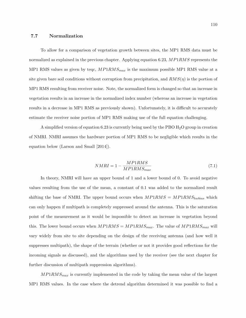
110

7.7 Normalization

To allow for a comparison of vegetation growth between sites, the MP1 RMS data must be

normalized as explained in the previous chapter. Applying equation 6.23, MP1RMS represents the

MP1 RMS values as given by teqc, MP1RMSmax is the maximum possible MP1 RMS value at a

site given bare soil conditions without corruption from precipitation, and RMS(η) is the portion of

MP1 RMS resulting from receiver noise. Note, the normalized form is changed so that an increase in

vegetation results in an increase in the normalized index number (whereas an increase in vegetation

results in a decrease in MP1 RMS as previously shown). Unfortunately, it is difficult to accurately

estimate the receiver noise portion of MP1 RMS making use of the full equation challenging.

A simplified version of equation 6.23 is currently being used by the PBO H2O group in creation

of NMRI. NMRI assumes the hardware portion of MP1 RMS to be negligible which results in the

equation below (Larson and Small [2014]).

NMRI = 1− MP1RMS

MP1RMSmax(7.1)

In theory, NMRI will have an upper bound of 1 and a lower bound of 0. To avoid negative

values resulting from the use of the mean, a constant of 0.1 was added to the normalized result

shifting the base of NMRI. The upper bound occurs when MP1RMS = MP1RMShwbias which

can only happen if multipath is completely suppressed around the antenna. This is the saturation

point of the measurement as it would be impossible to detect an increase in vegetation beyond

this. The lower bound occurs when MP1RMS = MP1RMSmax. The value of MP1RMSmax will

vary widely from site to site depending on the design of the receiving antenna (and how well it

suppresses multipath), the shape of the terrain (whether or not it provides good reflections for the

incoming signals as discussed), and the algorithms used by the receiver (see the next chapter for

further discussion of multipath suppression algorithms).

MP1RMSmax is currently implemented in the code by taking the mean value of the largest

MP1 RMS values. In the case where the detrend algorithm determined it was possible to find a

111

baseline, the mean is taken of the top 25% of the MP1 RMS values. In the case where it is not

possible to find a baseline, only the top 5% is used as the top 25% frequently includes large portions

of the green-up and senescence phases of the growth cycle. It is necessary to use the mean of a

range of the top values to avoid outliers and to account for the variance seen in base values as a

result of the variance in the hardware induced noise in MP1 RMS.

The evolution of data from unprocessed MP1 RMS to NMRI can be seen in Figure 7.28 for

station p085. The growth cycle of green-up, peak vegetation, and senescence can be clearly seen in

the NMRI results.

Figures 7.29 through 7.31 show comparisons of average NMRI and NDVI at stations charac-

terized by location and vegetation types. The NMRI index exhibits good consistency with NDVI

for all three locations which attests to its usefulness for differenct climate and vegetation types. A

more detailed correlation is shown in figures 7.32 through 7.34. The correlation plots show results

for the original NMRI data as well as NMRI lagged by the number of days for the highest possible

correlation (14 days in the northwest, 13 days in the north, and 7 days in the southwest). The

lag reflects the difference between measuring ”greeness” (which NDVI days) and vegetation water

content (for NMRI). Adjusting for this difference in measurement methods at these sites results in

an 80% to 90% correlation between NDVI and NMRI.

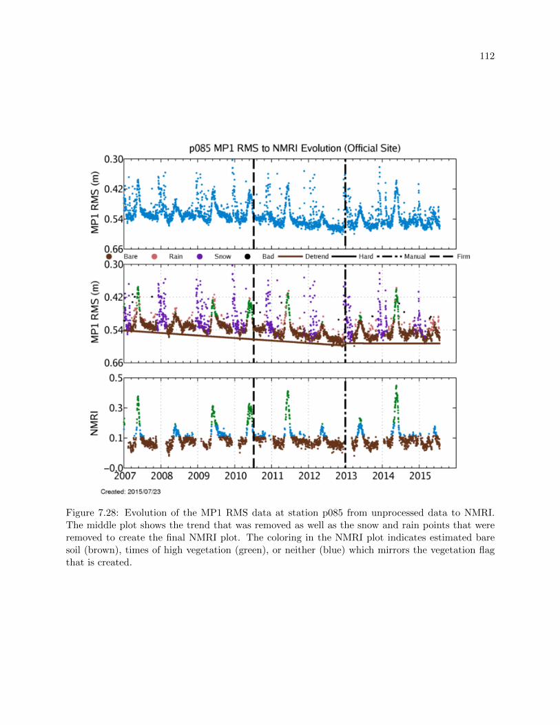
112

Figure 7.28: Evolution of the MP1 RMS data at station p085 from unprocessed data to NMRI.The middle plot shows the trend that was removed as well as the snow and rain points that wereremoved to create the final NMRI plot. The coloring in the NMRI plot indicates estimated baresoil (brown), times of high vegetation (green), or neither (blue) which mirrors the vegetation flagthat is created.

113

Figure 7.29: Comparison of average NDVI and NMRI at sites in northern California, Washington,and Oregon consisting mostly of grassland vegetation.

114

Figure 7.30: Comparison of average NDVI and NMRI at sites in Idaho, Montana, and Wyomingconsisting mostly of grassland vegetation.

115

Figure 7.31: Comparison of average NDVI and NMRI at sites in southern California, Nevada, andUtah consisting mostly of shrubland vegetation.

116

Figure 7.32: Correlation between average NDVI and NMRI at sites in northern California, Wash-ington, and Oregon consisting mostly of grassland vegetation. The NMRI data were lagged by 14days for the adjusted points.

Figure 7.33: Comparison of average NDVI and NMRI at sites in Idaho, Montana, and Wyomingconsisting mostly of grassland vegetation. The NMRI data were lagged by 13 days for the adjustedpoints.

117

Figure 7.34: Comparison of average NDVI and NMRI at sites in southern California, Nevada, andUtah consisting mostly of shrubland vegetation. The NMRI data were lagged by 7 days for theadjusted points.

118

7.8 Published Products

The PBO H2O group currently offers a version 1 NMRI product for 336 stations throughout

the western United States and Alaska (with a few sites in other locations). This product is based

on the original group filtering, detrending, and normalization algorithms. NMRI is part of a group

of products that are offered by the PBO H2O group (at http://xenon.colorado.edu/portal/) as a

public service to hyrdrologists and other scientists who work in studying snow, soil moisture, plant

growth, and similar areas.

Version 2 of the NMRI products will be based on the algorithms detailed in this chapter. The

new vegetation product will have enhanced filtering and detrending and there will be 3 additional

products provided. One of these products will be the vegetation flag, that was mentioned in the

detrending section, which will lead to more accurate soil moisture products. There will also be

two new versions of NMRI. The first, called iNMRI, is an interpolated version of NMRI that

provides a variant of the vegetation index where the data is smoothed over an interval of 7 days

and interpolated on days that are removed for snow and rain from the traditional product. The

second new product is called tNMRI and is a temperature corrected version of the original. The

method for doing this is outlined in the next chapter.

The transition from version 1 to version 2 NMRI will also include the addition of 185 stations

that show improved vegetation estimation as a result of the different algorithms used to calculate

NMRI. The increased number of stations will provide coverage in new areas as well as improving

coverage in areas for which data are already available. Figure 7.35 shows the location of the old

and new official vegetation sites.

119

Figure 7.35: The official sites for the vegetation products provided by the PBO H2O group. Thenew sites will become active with the second generation of products.

Chapter 8

Secondary noise sources in the MP1 RMS data

The previous chapter covered the major topics in the preparation of the MP1 RMS data

for use as a vegetation index. Some less typical effects, however, need to be considered as well

for optimal performance. This chapter discusses the influence of these effects and their possible

mitigation.

8.1 Temperature effects on the MP1 RMS data

Ambient temperature can have a large effect on noise levels in GPS receivers. Although

the MP1 signal is primarily viewed as an indicator of the magnitude of multipath incident on an

antenna, receiver noise is also a factor in the measurement. The effect of the receiver noise is

generally limited to a trend in the MP1 RMS as detailed in the previous section. At sites, however,

where receiver noise varies considerably at time spans of less than a year or where multipath does

not show significant variation, the change in MP1 comes to be dominated by the receiver noise

term.

The effect of ambient temperature on receiver noise and MP1 RMS can be seen at some of

the PBO sites analyzed for this study. Figure 8.1 shows a comparison between MP1 RMS and

both NDVI and average ambient temperature for a site in southern California (p610). Typically

it has been shown in this dissertation that MP1 RMS correlates well with NDVI (i.e. figure 7.1),

but in this case it is evident that there is a much stronger correlation with the average ambient

temperature (calculating the two correlations shows that MP1 RMS has a correlation of 0.92 with

121

temperature but a correlation coefficient of only -0.5 with the NDVI). The result is dependent on

the receiver and the temperature ranges experienced. Figure 8.2 shows another site near the first

that has no temperature correlation despite similar conditions to the first (the large variation in

NDVI for this site is a result of fields near the station but outside the range of the GPS multipath).

Figure 8.1: Comparison of NDVI, MP1 RMS, and average temperature at p610 in southern Califor-nia. A strong correlation can be seen between the temperature and MP1 RMS data. The negativecorrelation between the NDVI and MP1 RMS data is much smaller. For this site, temperature isobviously driving the change in MP1 RMS.

Of the evaluated sites, roughly 12% exhibited a large enough correlation (greater than 0.65)

between the MP1 RMS and the average temperature to be suspect. This number, though, is higher

than the actual number of sites being dominated by the temperature effect because plant growth

can also be correlated with temperature resulting in false positives. This is likely the case at p273

shown in figure 8.3 where the average temperature correlates well with both MP1 RMS (ρ = 0.70)

and NDVI (ρ = -0.49).

Although the correlation between temperature and MP1 RMS over long time intervals is

122

Figure 8.2: Comparison of NDVI, MP1 RMS, and average temperature at p563 in southern Cali-fornia. There is no strong correlation between MP1 RMS and either NDVI or average temperature.

Figure 8.3: Comparison of NDVI, MP1 RMS, and average temperature at p273 in northern Cali-fornia. There is a strong correlation between MP1 RMS and both NDVI and average temperature.

123

a poor indication of the effect of temperature on the data, the correlation between short term

variations in temperature and MP1 RMS can be used to mitigate temperature effects on the MP1

RMS data. The temperature can vary much more rapidly than the vegetation water content on 2

week time scales. Comparing the variation of MP1 RMS over this interval to the temperature gives

a much clearer indication of the temperature bias on the data. The top plot in figure 8.4 shows

the raw MP1 RMS data colored by the variation in temperature using a one week moving average.

It can be clearly seen that cooler temperatures tend to exhibit slightly lower MP1 RMS values

and higher relative temperatures exhibit higher MP1 RMS values. Fitting a least squares to the

correlation between the variation in temperature and variation in MP1 RMS over 1 week intervals

(as seen in the lower left plot of the same figure) a value can be fixed on the effect of the temperature

on the MP1 RMS data. The second plot in the figure shows the MP1 RMS data after this effect

has been removed using the value determined via least squares. The data clearly exhibits a much

better correlation with the NDVI values (see figure 8.5) and a much smaller sinusoidal signal that

was being driven by the temperature. The coloring of the points in the second figure also seems to

indicate that the noise remaining in the MP1 RMS data is much less dependent on temperature.

Two other representative examples are shown in figures 8.6 through 8.9 for stations p014 and

p273 respectively. p014 is also known to have a strong temperature effect whereas it was postulated

above that the correlation with temperature for p273 was mostly driven by the correlation between

plant growth and temperature. The results for p014 are similar to those of p610 where there is

a significant correlation between the variations over the short term and the MP1 RMS data more

closely correlates with the NDVI following the attempted temperature removal. For p273, however,

there is a much smaller correlation between the short term variations and the MP1 RMS data

before and after are nearly identical. This would support the idea that p273 is not being heavily

influenced by temperature and the temperature removal algorithm is not adding noticeable noise

for stations that are not strongly influenced by temperature.

The above examples are representative of stations in general. Sites that exhibited heavy

temperature influence had much of that removed with this method and those that didn’t were largely

124

Figure 8.4: Summary of the temperature effect on the MP1 RMS data for p610. The top plot showsthe raw MP1 RMS data colored by the 1 week temperature variation with the second plot showingMP1 RMS after the effect has been mostly removed. The NDVI is shown for comparison. Thebottom two plots show correlation between weekly variation in the MP1 RMS and temperaturebefore and after the effect is removed.

left untouched. Many of the sites that showed large temperature influences were mostly barren and

very flat which resulted in little vegetation signal even after the removal of the temperature effect,

however, there were some sites that proved viable for vegetation measurement after applying this

algorithm.

125

Figure 8.5: Correlation between NMRI and NDVI before and after an attempted temperaturecorrection to the NMRI data for p610. There is an increase in correlation after the temperatureremoval.

126

Figure 8.6: Summary of the temperature effect on the MP1 RMS data for p014 in southern Arizona.The top plot shows the raw MP1 RMS data colored by the 1 week temperature variation with thesecond plot showing MP1 RMS after the effect has been mostly removed. The NDVI is shown forcomparison. The bottom two plots show correlation between weekly variation in the MP1 RMSand temperature before and after the effect is removed.

127

Figure 8.7: Summary of the temperature effect on the MP1 RMS data for p273. The top plotshows the raw MP1 RMS data colored by the 1 week temperature variation with the second plotbeing the corrected MP1 RMS. The NDVI is shown for comparison. The bottom two plots showcorrelation between weekly variation in the MP1 RMS and temperature before and after the effectis removed. There is little change at this station.

128

Figure 8.8: Correlation between NMRI and NDVI before and after an attempted temperaturecorrection to the NMRI data for p014. There is a signficant increase in correlation after thetemperature removal.

Figure 8.9: Correlation between NMRI and NDVI before and after an attempted temperaturecorrection to the NMRI data for p273. There is a small change in correlation after the temperatureremoval.

129

8.2 Multipath supression algorithms

As mentioned in Chapter 5 there are methods for designing the receiver architecture that

will assist in the minimization of multipath. These methods are patented by the various GPS

manufacturers which frequently makes it difficult to know exactly what the algorithms are doing

but they typically involve the use of multiple correlators. For instance, the Trimble patented Everest

multipath suppression algorithm at least partly involves the estimation of the multipath delay and

phase by the use of a least-squares comparison between the expected correlation peak and the actual

correlation peak as seen by several correlators [Enge et al., 1997]. The many correlators allow the

identification or local peaks in the comparison between expected and actual signal correlation.

The suppression of the multipath through these algorithms is obviously of concern to this

research as it is based on measuring multipath from geodetic receivers deployed for geoscience

applications. However, there are two factors that mitigate much of the concern. The first is that,

as a result of the clandestine nature of these algorithms, many GPS networks suggest or require

that the algorithms be deactivated at their sites. For instance, the IGS network’s site guidlines

stipulate that “Multipath mitigation should be disabled in the GNSS receiver. In any case, the

receiver settings in this regard shall be reported via the station log.” [Infrastructure Committee

Central Bureau, 2013]

The second mitigating factor is that multipath suppression reduces, but does not remove,

the magnitude of the MP1 signal. To demonstrate this we asked UNAVCO to activate the Everest

multipath suppression algorithm at p048 in 2013 for day of year 297 and at p042 and p208 for day

of year 305. Figures 8.10 through 8.12 show a comparison of the daily MP1 RMS for the day with

the algorithm turned on and a neighboring day when the algorithm was turned off. In each case

the general features or hotspots for the MP1 RMS remained the same but the overall magnitude

lessened. Figure 8.13, which shows a comparison of MP1 for a single PRN, further emphasizes this.

As in the other plots it is apparent that the multipath is reduced but azimuth changes in multipath

are still evident. As can be seen, even with multipath suppression turned on, it would be possible

130

to make measurements of the multipath environment, though a year long test at several sites would

be needed to better assess the complete impact.

Figure 8.10: Comparison of MP1 with and without multipath suppression at p042 in easternWyoming. The MP1 RMS has the same general features but a lower magnitude when the suppres-sion algorithm is used.

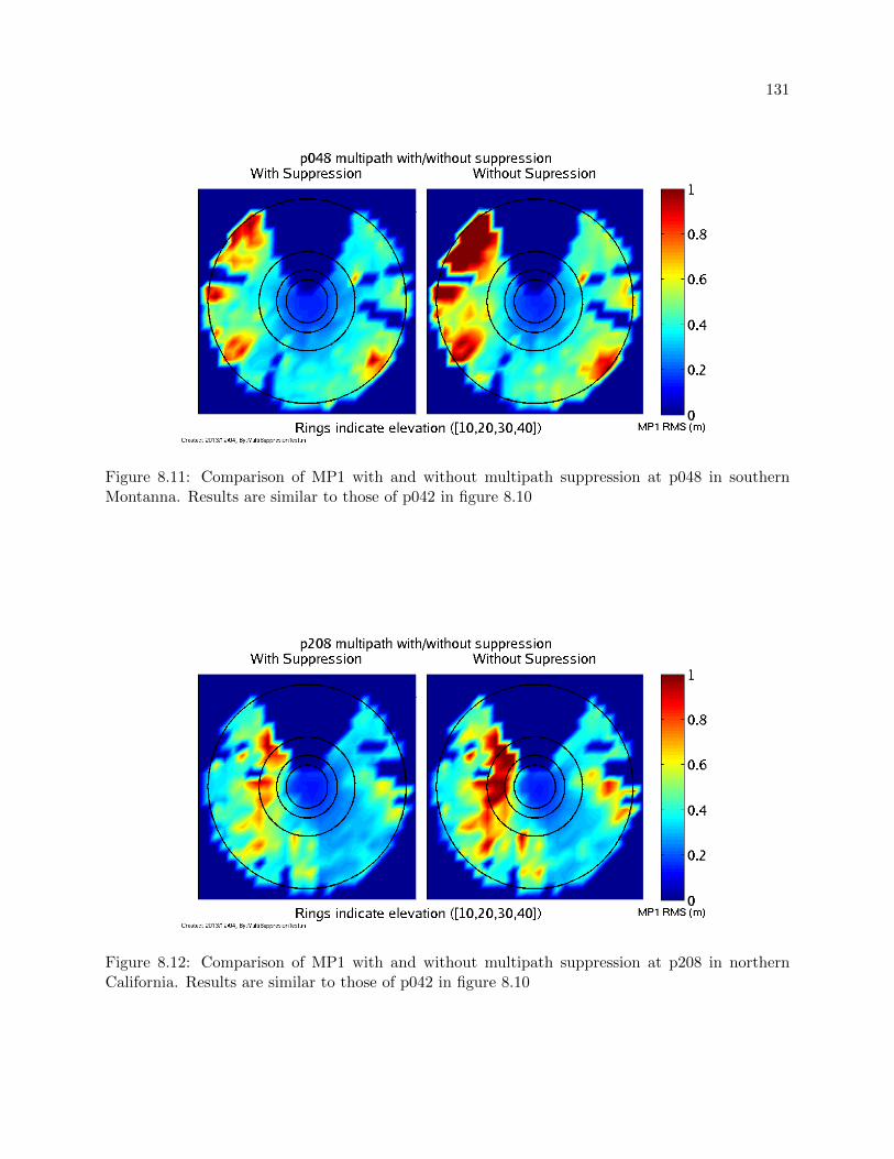
131

Figure 8.11: Comparison of MP1 with and without multipath suppression at p048 in southernMontanna. Results are similar to those of p042 in figure 8.10

Figure 8.12: Comparison of MP1 with and without multipath suppression at p208 in northernCalifornia. Results are similar to those of p042 in figure 8.10

132

Figure 8.13: Comparison of MP1 with and without multipath suppression at p048 for PRN 1.The MP1 for both days is similar though the suppressed multipath is smaller at low elevations,especially in the northwest quadrant where the best reflector is located.

Chapter 9

Summary and Future Work

The use of global navigation satellite systems is rapidly expanding in our society in a number

of ways, both commercial and scientific. This will only continue as more of these systems come on-

line in the near future. Realizing the potential of these systems for the great boon they can provide

to scientific research will speed progress in many different areas. The research in this dissertation

has detailed two of those areas, timing and remote sensing, and the summaries below highlight the

conclusions.

9.1 Periodic Representations of Navigation Satellite Clocks

The work on periodic variations in the GPS satellite clocks showed conclusively that the

magnitudes of the periodic components are sufficiently small compared to the overall estimation

noise that no extra terms are required in the broadcast message. Although modeling of the periodic

components is important in the prediction of the clock biases, the current 2-hour linear model has

modeling errors significantly smaller than the error in the prediction itself.

9.2 High Integrity GPS

The work outlined in this paper provides a reliable basis on which to estimate the Iridium

satellite clocks for such a system. The next step in the development of the Iridium global clock

estimator would be to focus on improving the overall accuracy and short-term precision of the

results. Downlink biases can be better estimated by increasing the number of ground stations

134

which will allow for an accurate estimate of the bias of each ground station relative to the mean.

The mean bias can then be calibrated through hardware measurements at one or two of the ground

stations. Clock drifts can be better estimated by incorporating high-precision phase measurements

from the crosslinks (UWPs) and the downlinks. Again, special attention is required to provide

the best possible accuracy with rapid response to discrete adjustments of a satellite clock bias or

frequency. Downlink phase measurements were made and incorporated into the reference receiver

which would support this effort. Once they are reliably established, improvements to the clock drift

estimates could be integrated with the bias measurements to further improve the performance of

the clock bias filter.

9.3 Measurement of vegetation using MP1 RMS

The PBO H2O group continues to expand on the products available both in quantity and

quality. Improvements are being made to all of the products offered. The work in this dissertation

details many of the improvements being made to the vegetation portion of the offered products.

The products have the potential to greatly facilitate many scientific fields, particularly in climate

research, and represent a vast body of untapped data. In its current iteration, NMRI has many

qualities that recommend it for use with or instead of NDVI which include improved temporal

resolution, less atmospheric interference, and a smaller footprint.

Although NMRI is usable in its current format, an improvement to the normalization could

greatly increase the use of NMRI for cross-site comparisons. Improved methods for estimating

GPS receiver noise would greatly facilitate this work. More detailed research in the hardware based

portion of MP1 RMS might also reveal improved methods of removing trends in these measurement

tools.

Finally, advances in terrain-based GPS reflection coefficients would allow for estimation of

MP1 RMS variability regardless of the availability of baselines. This could greatly increase the

usefulness of a GPS based vegetation water content index in locations with heavy snowfall. All of

these improvements would not only advance the use of GPS as a remote sensing tool but could

135

prove to advance more basic GPS uses through an increased understanding of multipath.

Bibliography

David Allan and James Barnes. Optimal time and frequency transfer using GPS signals. InProceedings of the 36th Annual Frequency Control Symposium, page 378. IEEE, 1982. doi:10.1109/FREQ.1982.200599.

David W. Allan, Neil Ashby, and Clifford C. Hodge. The Science of Timekeeping. Hewlett Packard,1997. Application Note 1289.

Thomas Bahder. Correlations between GPS and USNO master clock time. IEEE Transactions onAerospace and Electronic Systems, 34(4), 1998. doi: 10.1109/7.722720.

James Barnes. An adaptive algorithm to evaluate clock performance in real time. In Proceedingsof the 20th Annual Precise Time and Time Interval Applications and Planning Meeting, page205. PTTI, 1988.

Andria L. Bilich. Improving the precision and accuracy of geodetic GPS: Applications to multipathand seismology. Ph.D. Thesis, University of Colorado - Boulder, 2006.

Adrian A Borsa, Jean-Bernard Minster, Bruce G bills, and Helen A Fricker. Modeling long-periodnoise in kinematic GPS applications. Journal of Geodesy, 81(2), 2007. doi: 10.1007/s00190-006-0097-x.

Michael S Braasch. Multipath effects. In Brad Parkinson, James Spilker, Penina Axelrad, and PerEnge, editors, Global Positioning System: Theory and Applications, page 547. AIAA, 1996.

E Cardellach, F Fabra, O Nogues-Correig, S Oliveras, S Ribo, and A Rius. GNSS-R ground-based and airborne campaigns for ocean, land, ice, and snow techniques: Application to theGOLD-RTR data sets. Radio Science, 46, 2011. doi: 10.1029/2011RS004683.

James Chaffee. Observability, ensemble averaging and GPS time. IEEE Transactions on Aerospaceand Electronic Systems, 28(1), 1992. doi: 10.1109/7.135448.

Clara C Chew, Eric E Small, Kristine M Larson, and Valery U Zavorotny. Vegetation sensingusing GPS-interferometric reflectometry: Theoretical effects of canopy parameters on signal-to-noise ratio data. IEEE Transactions on Geoscience and Remote Sensing, 53(5), 2014. doi:10.1109/TGRS.2014.2364513.

Nicola Clerici, Christof J Weissteiner, and France Gerard. Exploring the use of MODIS NDVI-based phenology indicators for classifying forest general habitat categories. Remote Sensing, 4(6), 2012. doi: 10.3390/rs4061781.

137

Steven F Clifford, Valerian I Tatarskii, Alexander G Voronovich, and Valery U Zavorotny. GPSsounding of ocean surface waves: theoretical assessment. Geoscience and Remote SensingSymposium Proceedings, 4, 1998. doi: 10.1109/IGARSS.1998.703722.

Peter B. Coates. Frequency measurement. In AccessScience. McGraw-Hill Companies, 2014.

G. Dall’olmo and A. Karnieli. Monitoring phenological cycles of desert ecosystems using NDVI andLST data derived from NOAA-AVHRR imagery. International Journal of Remote Sensing, 23(19), 2002. doi: 10.1080/01431160110115988.

J.A. Davis, C.A. Greenhall, and P.W. Stacey. A Kalman filter clock algorithm for use in the presenceof flicker frequency modulation noise. Metrologia, 42(1), 2005. doi: 10.1088/0026-1394/42/1/001.

A J Van Dierendonck, J B McGraw, and R Grover Brown. Relationship between Allan variancesand Kalman filter parameters. In Proceedings of the 16th Annual Precise Time and Time IntervalApplications and Planning Meeting, page 273. PTTI, 1984.

P. Enge, D. Farmer, and J.F. Schipper. Adaptive multipath equalization, May 13 1997. URLhttp://www.google.com/patents/US5630208. US Patent 5,630,208.

Louis H Estey and Charles M Meertens. TEQC: The multi-purpose toolkit for GPS/GLONASSdata. GPS Solutions, 3(1), 1999. doi: 10.1007/PL00012778.

Sarah G Evans, Eric E Small, and Kristine M Larson. Comparison of vegetation phenology in thewestern USA determine from reflected GPS microwave signals and NDVI. Internation Journalof Remote Sensing, 35(9), 2014. doi: 10.1080/01431161.2014.894660.

Carl Foosa, Richard Raines, Gregg Gunsch, and Michael Temple. An overview of the IRIDIUM R©

low earth orbit LEO satellite system. In Proceedings of the IEEE 1998 National Aerospace andElectronics Conference, page 152. IEEE, 1998. doi: 10.1109/NAECON.1998.710110.

Scott Gleason, Mounir Adjrad, and Martin Unwin. Sensing ocean, ice and land reflected signalsfrom space: Results from the UK-DMC GPS reflectometry experiment. In Proceedings of the18th International Technical Meeting of the Satellite Division of The Institute of Navigation,page 1679. ION GNSS, 2005.

GPS Reflections Group. PBO H2O data portal. http://xenon.colorado.edu/portal. Last accessedFebruary 1, 2015.

Charles Greenhall. Kalman plus weights: A time scale algorithm. In Proceedings of the 33rdAnnual Precise Time and Time Interval Meeting, page 445. PTTI, 2001.

Charles Greenhall. A Kalman filter clock ensemble algorithm that admits measurement noise.Metrologia, 43(4), 2006. doi: 10.1088/0026-1394/43/4/S19.

Ethan D Gutmann, Kristine M Larson, Mark W Williams, Felipe G Nievinski, and Valery Za-vorotny. Snow measurement by GPS interferometric reflectometry: an evaluation at NiwotRidge, Colorado. Hydrological Processes, 26(19), 2011. doi: 10.1002/hyp.8329.

Bruce M Hannah. Modeling and simulation of GPS multipath propagation. Ph.D. Thesis, Queens-land University of Technology, 2001.

138

Youn Jeong Heo, Jeongho Cho, and Moon Beom Heo. Improving prediction accuracy of GPSsatellite clocks with periodic variation behaviour. Measurement Science and Technology, 21(7),2010. doi: 10.1088/0957-0233/21/7/073001.

Bernhard Hofman-Wellenhof, Herbert Lichtenegger, and James Collins. Global Positioning SystemTheory and Practice. Springer, 5th edition, 2001.

Infrastructure Committee Central Bureau. IGS Site Guidelines. International GNSS Service, 2013.Available at https://igscb.jpl.nasa.gov/network/guidelines/guidelines.html.

Interface Specification, Revision G. Navstar GPS space segment/navigation user interfaces.http://www.gps.gov/technical/icwg/IS-GPS-200G.pdf. Last accessed September 1, 2012.

International GNSS Service. IGS products. http://igscb.jpl.nasa.gov/components/prods.html. Lastaccessed July 1, 2009.

Michael E Jackson. Geophysics at the speed of light: EarthScope and the Plate Boundary Obser-vatory. The Leading Edge, 22(3), 2003. doi: 10.1190/1.1564532.

Shuanggen Jin, Estel Cardellach, and Feiqin Xie. GNSS Remote Sensing. Springer, 1st edition,2014.

Mathieu Joerger, Jason Neale, and Boris Pervan. Iridium GPS carrier phase positioning and faultdetection over wide areas. In Proceedings of the 22nd International Technical Meeting of theSatellite Division of the Institute of Navigation. Institute of Navigatin, 2009.

Mathieu Joerger, Livio Gratton, Boris Pervan, and Clark E Cohen. Analysis of iridium-augmentedGPS for floating carrier phase positioning. Navigation, 57(2), 2010. doi: 10.1002/j.2161-4296.2010.tb01773.x.

Richard Jones and Peter Tryon. Continuous time series models for unequally spaced data appliedto modeling atomic clocks. SIAM Journal on Scientific and Statistical Computing, 8(1), 1987.doi: 10.1137/0908007.

Stephen J Katzberg, Omar Torres, Michael S Grant, and Dallas Masters. Utilizing calibratedGPS reflected signals to estimate soil reflectivity and dielectric constant: Results from SMEX02.Remote Sensing of Environment, 100(1), 2006. doi: 10.1016/j.rse.2005.09.015.

Kristine M Larson and Felipe G Nievinski. GPS snow sensing: results from the Earthscope PlateBoundary Observatory. GPS Solutions, 17(1), 2013. doi: 10.1007/s10291-012-0259-7.

Kristine M Larson and Eric E Small. Normalized microwave reflection index: A vegetation mea-surement derived from GPS networks. IEEE Journal of Selected Topics in Applied EarthObserverations and Remote Sensing, 7(5), 2014. doi: 10.1109/JSTARS.2014.2300116.

Kristine M Larson, Eric E Small, Ethan Gutmann, Andria Bilich, Penina Axelrad, and John Braun.Using GPS multipath to measure soil moisture fluctuations: initial results. GPS Solutions, 12(3), 2008. doi: 10.1007/s10291-007-0076-6.

Kristine M Larson, Ethan D Gutmann, Valery Zavorotny, John J Braun, Mark W Williams, andFelipe G Nievinski. Can we measure snow depth with GPS receivers? Geophysical ResearchLetters, 36, 2009. doi: 10.1029/2009GL039430.

139

Kristine M Larson, John J Braun, Eric E Small, Valery U Zavorotny, Ethan D Gutmann, andAndria L Bilich. GPS multipath and its relation to near-surface soil moisture content. IEEEJournal of Selected Topics in Applied Earth Observations and Remote Sensing, 3(1), 2010. doi:10.1109/JSTARS.2009.2033612.

Kristine M Larson, Johan S Lofgren, and Rudiger Haas. Coastal sea level measurementsusing a single geodetic GPS receiver. Advances in Space Research, 51(8), 2013a. doi:10.1016/j.asr.2012.04.017.

Kristine M Larson, Richard D Ray, Felipe G Nievinski, and Jeffrey T Freymueller. The accidentaltide gauge: A GPS reflection case study from Kachemak Bay, Alaska. IEEE Geoscience andRemote Sensing Letters, 10(5), 2013b. doi: 10.1109/LGRS.2012.2236075.

Kristine M Larson, Eric E Small, and William Kolby Smith. Normalized microwave reflection index:Validation of Vegetation Water Content from Montana grasslands. IEEE Journal of SelectedTopics in Applied Earth Observerations and Remote Sensing, 7(5), 2014. doi: 10.1109/JS-TARS.2014.2320597.

Pratap Misra and Per Enge. Global Positioning System: Signals, Measurements, and Performance.Ganga-Jamuna Press, 2nd edition, 2006.

Kenneth E Mitchell, Dag Lohmann, Paul R Houser, Eric F Wood, John C Schaake, Alan Robock,Brian A Cosgrove, Justin Sheffield, Qingyun Duan, Lifeng Luo, R Wayne Higgins, Rachel TPinker, J Dan Tarpley, Dennis P Lettenmaier, Curtis H Marshall, Jared K Entin, Ming Pan, WeiShi, Victor Koren, Jesse Meng, Bruce H Ramsay, and Andrew A Bailey. The multi-institutionNorth American land data assimilation system (NLDAS): Utilizing multiple gcip products andpartners in a continental distributed hydrological modeling system. Journal of GeophysicalResearch: Atmospheres, 109(D7), 2004. doi: 10.1029/2003JD003823.

MODIS Land. MODIS products. http://modis-land.gsfc.nasa.gov. Last accessed October 1, 2013.

Oliver Montenbruck, Urs Hugentobler, Rolf Dach, Peter Steigenberger, and Andre Hauschild. Ap-parent clock variations of the block IIF-1 (SVN62) GPS satellite. GPS Solutions, 16(3), 2011.doi: 10.1007/s10291-011-0232-x.

Navigation National Coordination Office for Space-Based Positioning and Timing. GPS Applica-tions. http://www.gps.gov/applications/. Last accessed April 1, 2012.

Felipe G Nievinski and Kristine M Larson. An open source GPS multipath simulator in Mat-lab/Octave. GPS Solutions, 18(3), 2014. doi: 10.1007/s10291-014-0370-z.

NIST. Time and frequency: From A to Z. http://tf.nist.gov/general/glossary.htm. Last accessedApril 1, 2012.

John Pratt, Penina Axelrad, Kristine M Larson, Bruno Lesage, Richard Gerren, and NicholasDiOrio. Satellite clock bias estimation for iGPS. GPS Solutions, 17(3), 2012. doi: 10.1007/s10291-012-0286-4.

George A Riggs, Dorothy K Hall, and Vincent V Salomonson. MODIS Snow Products User Guideto Collection 5. The MODIS Snow and Sea Ice Global Mapping Project, 2006. Available athttp://modis-snow-ice.gsfc.nasa.gov/uploads/sug c5.pdf.

140

W.J. Riley. Handbook of Frequency Stability Analysis. NIST, 2008. NIST Special Publication1065.

Matthew Rodell. LDAS land data assimilation systems. http://ldas.gsfc.nasa.gov/index.php. Lastaccessed October 1, 2013.

C Ruf, A Lyons, M Unwin, J Dickinson, R Rose, D Rose, and M Vincent. CYGNSS: Enablingthe future of hurricane prediction. Geoscience and Remote Sensing Magazine, 1(2), 2013. doi:10.1109/MGRS.2013.2260911.

J. Schuss, J. Upton, B. Myers, T. Sikina, A. Rohwer, P. Makridakas, R. Francois, L. Wardle, andR. Smith. The IRIDIUM main mission antenna concept. IEEE Transactions on Antennas andPropagation, 47(3), 1999. doi: 10.1109/8.768775.

Mark D Schwartz, editor. PHENOLOGY: An Integrative Environmental Science. Kluwer AcademicPublishers, 1st edition, 2003.

Kenneth Senior, Paul Koppang, and Jim Ray. Developing an IGS time scale. IEEE Transactions onUltrasonics, ferroelectrics, and frequency control, 50(6), 2003. doi: 10.1109/FREQ.2001.956188.

Kenneth Senior, Jim Ray, and Ronald Beard. Characterization of periodic variations in the GPSsatellite clocks. GPS Solutions, 12(3), 2008. doi: 10.1007/s10291-008-0089-9.

Yuriy Shmaliy and Oscar Ibarra-Manzano. Studies of the unbiased FIR filter for the time errormodel in applications to GPS-based timekeeping. In Proceedings of the 36rd Annual PreciseTime and Time Interval Meeting, page 441. PTTI, 2004.

Yuriy Shmaliy, Oscar Ibarra-Manzano, and Luis Arceo-Miquel. A numerical comparison of theunbiased FIR and Kalman filters in applications to GPS-based timekeeping. In Proceedingsof the IEEE International Frequency Control Symposium, page 668. IEEE, 2005. doi:10.1109/FREQ.2005.1574015.

Eric E Small, Kristine M Larson, and John J Braun. Sensing vegetation growth with reflected GPSsignals. Geophysical Research Letters, 37(12), 2010. doi: 10.1029/2010GL042951.

Ramon Solano, Kamel Didan, Andree Jacobson, and Alfredo Huete. MODIS VegetationIndex User’s Guide. Vegetation Index and Phenology Lab, 2010. Available athttp://vip.arizona.edu/documents/MODIS/MODIS VI UsersGuide 01 2012.pdf.

S.R. Stein. Kalman filter analysis of precision clocks with real-time parameter estimation. InProceedings of the 43rd Annual Frequency Control Symposium, page 232. IEEE, 1989. doi:10.1109/FREQ.1989.68870.

S.R. Stein. Advances in time-scale algorithms. In Proceedings of the 24th Annual Precise Timeand Time Interval Applications and Planning Meeting, page 289. PTTI, 1992.

S.R. Stein. Time scales demystified. In Proceedings of the 2003 IEEE International FrequencyControl Symposium and PDA Exhibition Jointly with the 17th European Frequency and TimeForum, page 223. IEEE, 2003. doi: 10.1109/FREQ.2003.1275093.

141

S.R. Stein and John Evans. The application of Kalman filters and ARIMA models to the studyof time predictions errors of clocks for use in the defense communication system (DCS). InProceedings of the 44th Annual Symposium on Frequency Control, page 630. IEEE, 1990. doi:10.1109/FREQ.1990.177553.

S.R. Stein and R.L. Filler. Kalman filter analysis for real time applications of clocks and oscillators.In Proceedings of the 42nd Annual Frequency Control Symposium, page 447. IEEE, 1988. doi:10.1109/FREQ.1988.27638.

Everett Swift and Bruce Hermann. Orbit period frequency variations in the GPS satellite clocks.In Proceedings of the 20th Annual Precise Time and Time Interval Meeting, page 87. PTTI,1988.

Byron D Tapley, Bob E Schutz, and George H Born. Statistical Orbit Determination. ElsevierAcademic Press, 1st edition, 2004.

UNAVCO. UNAVCO Resources: GNSS Antennas. http://facility.unavco.org/kb/questions/458/UNAVCO+Resources:+GNSS+Antennas. Last accessed July 24, 2015.

USNO. Block II satellite information. ftp://tycho.usno.navy.mil/pub/gps/gpsb2.txt. Last accessedMarch 1, 2012.

Francine Vannicola, Ronald Beard, Joseph White, Kenneth Senior, Marie Largay, and James Buis-son. GPS block IIF atomic frequency standard analysis. In Proceedings of the 42nd AnnualPrecise Time and Time Interval Meeting, page 181. PTTI, 2010.

John R. Vig. Introduction to Quartz Frequency Standards. IEEE Ultrasonics, Fer-roelectrics, and Frequency Control Society, 1992. Available at http://www.ieee-uffc.org/frequency control/teaching.asp?vig=vigcomp.

Wolfgang Wagner, Vahid Naeimi, Klaus Scipal, Richard de Jeu, and Jose Martinez-Fernandez. Soilmoisture from operational meteorological satellites. Hydrogeology Journal, 15(1), 2007. doi:10.1007/s10040-006-0104-6.

Pierre Waller, F Gonzalez, J Hahn, S Binda, R Piriz, I Hidalgo, G Tobias, I Sesia, P Tabella,and G Cerretto. In-orbit performance assessment of GIOVE clocks. In Proceedings of the 40thAnnual Precise Time and Time Interval Applications and Planning Meeting, page 69. PTTI,2008.

Wikipedia. Moderate-resolution imaging spectroradiometer. http://en.wikipedia.org/wiki/MODIS.Last accessed September 1, 2013.

M L Williams, K M Fischer, J T Freymueller, B Tikoff, A M Trehu, et al. Unlocking the secrets ofthe North American continent: An EarthScope Science Plan for 2010-2020. February, 2010, 78pp.

Appendix A

Explanation of the modified Allan variance

The most commonly used variance for clock estimates is known as the Allan variance though

there are actually three types of Allan variances: the Allan variance, the overlapping Allan variance,

and the modified Allan variance. Most often, the overlapping Allan variance is known simply as the

Allan variance as the original does not always converge (depending on the noise in the clock) and

has no advantages over the overlapping variety. The modified Allan variance is able to distinguish

white and flicker phase noise but is more complex than the overlapping Allan variance. This follows

the derivation in Riley[Riley, 2008].

Let xi be the bias or phase of the clock at time ti where x has been evenly sampled in time

with interval τ . The frequency offset of the clock can then be defined as:

yi =xi+1 − xi

τ(A.1)

The Allan variance of a set of N bias measurements (which results in N-1 frequency estimates) is

defined as:

σ2y(τ) =

1

2(N − 2)

N−2∑i=1

[yi+1 − yi]2 (A.2)

This can be rewritten in terms of the bias:

143

σ2y(τ) =

1

2(N − 2)

N−2∑i=1

[xi+2 − xi+1

τ− xi+1 − xi

τ

]2

⇒ σ2y(τ) =

1

2(N − 2)τ2

N−2∑i=1

[xi+2 − 2xi+1 + xi]2 (A.3)

By using overlapping samples the stability of the calculation can be increased. Instead of

summing the square of the difference of the frequency at each interval, the sum of the square of

the mean overlapping frequency is used. This leads to the overlapping Allan variance (defined in

terms of the interval mτ):

σ2y(τ) =

1

2m2(N − 2m)

N−2m∑j=1

j+m−1∑i=j

[yi+m − yi]

2

(A.4)

As with the original Allan variance a form can be derived that uses the bias instead of the frequency:

σ2y(τ) =

1

2m2(N − 2m)τ2

N−2m∑j=1

j+m−1∑i=j

[xi+m+1 − xi+m − xi+1 + xi]

2

⇒ σ2y(τ) =

1

2m2(N − 2m)τ2

N−2m∑j=1

(xj+m+1 − xj+m − xj+1 + xj + xj+m+2 − xj+m+1

− xj+2 + xj+i + ...+ xj+2m − xj+2m−1 − xj+m + xj+m−1)2

⇒ σ2y(τ) =

1

2(N − 2m)τ2

N−2m∑j=1

(xj+2m − 2xj+m + xj)2 (A.5)

The bias version of the overlapping Allan variance has signficantly reduced computational intensity

because of the lack of a second summation so it is generally the preferred algorithm[Riley, 2008].

The final version of the Allan variance is the modified Allan variance. This form is frequently

use as it is the only one that can distinguish between white and flicker phase noise[Riley, 2008].

The values differ from the overlapping Allan variance at all noise types, however, so it is important

to indicate which type is being used. The modified Allan variance is defined as:

σ2y(τ) =

1

2m4(N − 3m+ 1)

N−3m+1∑k=1

k+m−1∑j=k

j+m−1∑i=j

[yi+m − yi]

2

(A.6)

144

The inner summation is the same as for the overlapping Allan variance so the bias version is:

σ2y(τ) =

1

2m2(N − 3m+ 1)τ2

N−3m+1∑k=1

k+m−1∑j=k

xj+2m − 2xj+m + xj

2

(A.7)

For any of the Allan variances the corresponding Allan deviation can be determined by

calculating the square root of the Allan variance.

Appendix B

Least Squares Estimation of Sine Waves

Let s(t) be defined as a signal composed using the two frequencies f1 and f2 and a quadratic.

s(t) can be written as:

s(t) = q0 + q1t+ q2t2 +A1 sin(ω1t+ φ1) +A2 sin(ω2t+ φ2) (B.1)

where qj represents the jth quadratic term and Ai, ωi, and φi are, respectively, the amplitude,

the angular frequency, and the phase of the ith frequency element. Using the summation of angles

identity for trigonometeric functions, s(t) can be written as:

s(t) = q0 + q1t+ q2t2 +A1 cos(φ1) sin(ω1t) +A1 sin(φ1) cos(ω1t) + ...

A2 cos(φ2) sin(ω2t) +A2 sin(φ2) cos(ω2t) (B.2)

The equation B.2 requires a non-linear estimation if Ai, φi, and ωi are all considered to be

unknowns. However, if it can be assumed that the frequencies f1 and f2 are known (as they are in

the GPS clock problem in Chapter 3) then the unknowns in equation B.2 are simplified to the four

amplitudes Ai cos(φi) and Ai sin(φi) for i = 1, 2. The resulting model is much simpler to estimate

and is an excellent candidate for a least-squares method. The state and matrix for the least-squares

system of equations is:

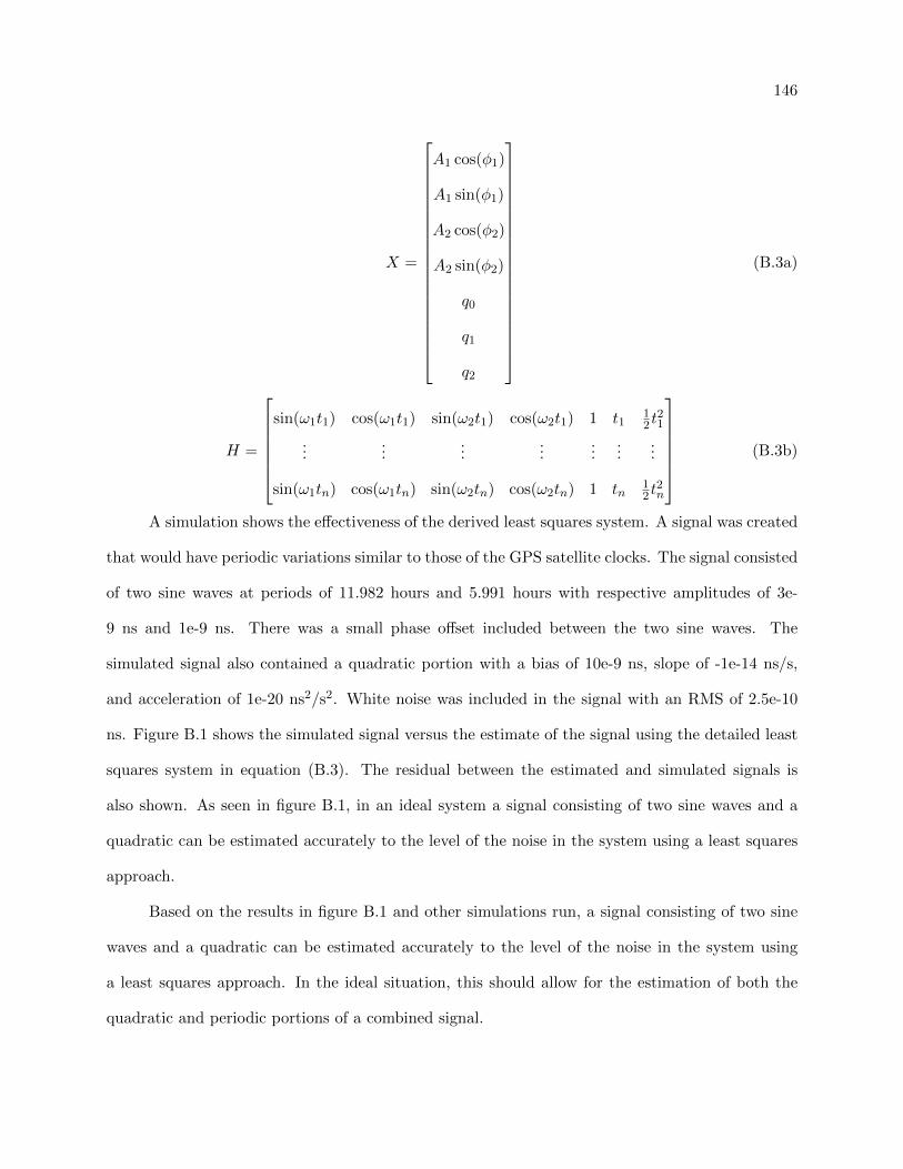
146

X =

A1 cos(φ1)

A1 sin(φ1)

A2 cos(φ2)

A2 sin(φ2)

q0

q1

q2

(B.3a)

H =

sin(ω1t1) cos(ω1t1) sin(ω2t1) cos(ω2t1) 1 t1

12 t

21

......

......

......

...

sin(ω1tn) cos(ω1tn) sin(ω2tn) cos(ω2tn) 1 tn12 t

2n

(B.3b)

A simulation shows the effectiveness of the derived least squares system. A signal was created

that would have periodic variations similar to those of the GPS satellite clocks. The signal consisted

of two sine waves at periods of 11.982 hours and 5.991 hours with respective amplitudes of 3e-

9 ns and 1e-9 ns. There was a small phase offset included between the two sine waves. The

simulated signal also contained a quadratic portion with a bias of 10e-9 ns, slope of -1e-14 ns/s,

and acceleration of 1e-20 ns2/s2. White noise was included in the signal with an RMS of 2.5e-10

ns. Figure B.1 shows the simulated signal versus the estimate of the signal using the detailed least

squares system in equation (B.3). The residual between the estimated and simulated signals is

also shown. As seen in figure B.1, in an ideal system a signal consisting of two sine waves and a

quadratic can be estimated accurately to the level of the noise in the system using a least squares

approach.

Based on the results in figure B.1 and other simulations run, a signal consisting of two sine

waves and a quadratic can be estimated accurately to the level of the noise in the system using

a least squares approach. In the ideal situation, this should allow for the estimation of both the

quadratic and periodic portions of a combined signal.

147

Figure B.1: Estimation of a simulated signal based on a quadratic and two sine waves at once andtwice the GPS orbital period. The simulated and estimated signals are shown in the top graph.The residuals between the estimated and generated signal are shown in the bottom graph. TheRMS of the residuals is 2.467e-10 ns while the simulated signal had included noise with an RMSof 2.5e-10 ns.

Appendix C

Estimation of the GPS Satellite Clocks

Typically, the bias on precision clocks is estimated using a quadratic model [Stein and Filler,

1988; Dierendonck et al., 1984]. As a result of the periodic nature of the GPS satellite clock bias,

the assumption that a quadratic model can return an optimal estimate of the satellite clocks must

be re-evaluated. It is shown below that, depending on the clock and time interval, more accurate

results can be achieved with an estimation scheme that includes periodic terms. The prediction

algorithm developed here for the GPS satellite clocks relies on a Kalman filter to estimate future

clock behavior based on past bias estimates. It incoporates the classic model as described by Stein

[Stein and Filler, 1988; Stein, 1989]. The classic model consists of three states: bias (b), frequency

offset (f), and frequency drift (d). To this are added four periodic terms AS1, AC1, AS2, and AC2

which represent amplitudes for periodic signals at once-per-orbit and twice-per-orbit respectively.

The filter state is defined as:

X =

b

f

d

AS1

AC1

AS2

AC2

(C.1)

At each epoch the filter estimates the state of the clock referenced to GPS time. The estimates

149

are propagated from one epoch to the next using the state transition matrix as shown in equation

(C.2).

X(t) = φ(t− t0)X(t0) (C.2a)

φ =

1 ∆t ∆t2 sin(ω1t) cos(ω1t) sin(ω2t) cos(ω2t)

0 1 ∆t 0 0 0 0

0 0 1 0 0 0 0

0 0 0 1 0 0 0

0 0 0 0 1 0 0

0 0 0 0 0 1 0

0 0 0 0 0 0 1

(C.2b)

The covariance of the state is also propagated using the standard Kalman filter equation

show in (C.3).

P (t) = φ(t− t0)P (t0)φ(t− t0)T +Qd (C.3)

where Qd represents the process noise in the dynamic model of the clock. The process noise is

defined below in (C.4).

150

Qd =

S0∆t+ S2∆t3

3 + S4∆t5

20 +Q11S2∆t2

2 + S4∆t4

8S4∆t3

6

S2∆t2

2 + S4∆t4

8 S2∆t+ S4∆t3

3S4∆t2

2

S4∆t3

6S4∆t2

2 S4∆t

−SA1 cos(ω1∆t)ω1

0 0

SA2 sin(ω1∆t)ω1

0 0


0 0

SA4 sin(ω2∆t)ω2

0 0

. . .


SA2 sin(ω1∆t)ω1


SA4 sin(ω2∆t)ω2

0 0 0 0

0 0 0 0

SA1∆t 0 0 0

0 SA2∆t 0 0

0 0 SA3∆t 0

0 0 0 SA4∆t

(C.4)

where

Q11 = −SA1 sin(2ω1∆t)− 2SA1ω1∆t

4ω1+SA2 sin(2ω1∆t) + 2SA2ω1∆t

4ω1− . . .

SA3 sin(2ω2∆t)− 2SA3ω2∆t

4ω2+SA4 sin(2ω2∆t) + 2SA4ω2∆t

4ω2(C.5)

The process noise dealing with the quadratic components of the state (the 3x3 matrix in

the top left of Qd) is defined with respect to the spectral noise densities of the clock: S0, S2, and

S4 (plus the Q11 term which deals with the periodic states). These terms are determined by the

white frequency, flicker frequency, and random walk frequency characteristics of the clock. The

values of the clock noise can be quantified using an Allan variance of the clock behavior over a long

interval [Stein and Filler, 1988; Dierendonck et al., 1984]. The process noise in the periodic states

is defined with respect to SA1, SA2, SA3, and SA4. These terms are more difficult to define as

the processes that drive the periodic effects are not as well understood. For the purposes of this

151

dissertation they were assigned a value scaled from the magnitude of the corresponding frequency

spectrum as generally clocks with more noise exhibited a larger periodic effect. The measurements

input to the filter are bias estimates of the clock. This can be implemented using standard Kalman

filter equations. The setup is trivial and therefore not shown here. The filter must be initialized

with at least 2 days of measurements before it can accurately predict the behavior of the satellite

clock. Once the filter has converged, predictions are stable for at least 24 hours following the last

measurement. The filter was tested using the same 30 day set that was discussed in Chapter 3.

Before testing the filter, the data set was used to calculate Allan variances for the satellite clocks

in order to generate the appropriate spectral noise densities for use with the filter. After each days

worth of measurements was processed by the filter, the filter state was used to predict the clock

bias for the next 24 hours. These predictions were compared to the IGS final clock biases. Three

different implementations of the filter were tested: one with all 7 states, one with the quadratic

states and the periodic states for the dominant once-per-orbit frequency, and one with just the

quadratic states. Figure C.1 shows errors in the predictions for PRN 16 on January 15th. The

error for the three different filter implementations is compared. As can be seen, even with periodic

parameters included in the prediction, it is difficult to remove the periodic effects when predicting

the satellite clock bias. This is due to variability present in the periodic signals from day to day.

However, using the estimation with periodic parameters does decrease the overall error in the

estimations over the long term and clock filters for space applications do use periodic terms in their

estimation.

152

Figure C.1: Comparison of the prediction error relative to IGS final clock solutions for 3 differentestimation methods. The predictions are based on the estimated state of the clock at the beginningof the day.

Appendix D

Kalman Filter Process Noise in Clock Bias Estimation

One of the most essential elements in correctly estimating the state and uncertainty in Kalman

filters is accurately sizing the noise in the propagation step of the filter. This quantity is known as

the process noise, Qd. It can be derived from the fundemantal Kalman equations. The basis for

these equations is from Tapley et al. [Tapley et al., 2004] (especially equation 4.9.44).

The X (which was defined in Chapter 3 as bias, frequency, and drift) is propagated via the

state trasition matrix:

φ =

1 ∆t 1

2∆t2

0 1 ∆t

0 0 1

(D.1)

The noise in the system is defined in terms of the spectral noise densities as shown below.

The noise is mapped to the state via the matrix B which, for this, case is the identity matrix due

to the assumption of independence in the different types of clock noise.

154

u =

√S0

√S2

√S4

(D.2)

Q = E(uuT ) =

S0 0 0

0 S2 0

0 0 S4

(D.3)

From this, the process noise for a discrete clock filter is derived:

Qd =

∫ tk

tk−1

φ(tk, τ)B(τ)Q(τ)BT (τ)φT (tk, τ)dτ

=

∫ tk

tk−1

1 ∆t 1

2∆t2

0 1 ∆t

0 0 1

S0 0 0

0 S2 0

0 0 S4

1 0 0

∆t 1 0

12∆t2 ∆t 1

dτ (∆t = tk − τ)

=

∫ tk

tk−1

S0 + S2∆t2 + 1

4S4∆t4 S2∆t+ 12S4∆t3 1

2S4∆t2

S2∆t+ 12S4∆t3 S4∆t2 + S2 S4∆t

12S4∆t2 S4∆t S4

dτ

=

S0∆t+ 1

3S2∆t3 + 120S4∆t5 1

2S2∆t2 + 18S4∆t4 1

6S4∆t3

12S2∆t2 + 1

8S4∆t4 S2∆t+ 13S4∆t3 1

2S4∆t2

16S4∆t3 1

2S4∆t2 S4∆t

(∆t = tk − tk−1) (D.4)

Appendix E

MODIS

MODIS is the moderate-resolution imaging spectroradiometer payload that NASA placed on

both the Terra and Aqua satellites launched in 1999 and 2002[Wikipedia]. The purposes of the

payloads were to monitor the change in global land surface characteristics. The satellites monitor

spectral bands ranging from 0.4 micrometers up to 14.4 micrometers from which various data

products are derived and provided to the public for research purposes. The various data products

that are provided are [MODIS Land]:

• Surface Reflectance

• Snow Cover/Sea Ice

• Land Surface Temperature

• Land Cover/Dynamics

• Vegetations Indices (NDVI/EVI)

• Thermal Anomalies/Fire

• Leaf Area Index/Fractional Photosynthetically Active Radiation

• Gross Primary Productivity

• Bidirectional Reflectance Distribution Function/Albedo

156

• Burned Area

The first day of MODIS science data acquisition was 24 February 2000 and most products

are available to that date. The data processing methods are periodically updated following which

the data is reprocessed so that older data have the same level of processing accuracy as new data

[Riggs et al., 2006]. The current processing methods are known as Collection 5.

The data products have various stages of processing know as level 1, 2, 3, or 4 products[Riggs

et al., 2006]. Only level 2 products and above are distributed with level 3 and 4 products being

intended for general use. Level 4 products are mostly a summary gleaned from the level 3 data.

During processing from level 1 to level 3 the products are cleaned for bad data, the pixels are given a

latitude/longitude location, cloud and coastal detection is done as well as various other processing.

The data are archived as Hierarchical Data Format - Earth Observing System files (HDF-EOS).

This is a binary representation developed by the National Center for Supercomputing Applications

and used by NASA in an attempt to standardize there distribution of geophysical products. The

file format not only includes the data but meta-data is built in which specifies which products are

in a file, where the pixel locations are, and what the header information is for each data product.

The NDVI data is of particular interest in this research. The satellites provide NDVI data

at a spatial resolution of 250 m. Although the temporal resolution of the data is less than a day,

the level 3 NDVI product has a temporal resolution of 16 days. All of the measurements inside

the 16 day window are processed to remove cloud and atmospheric corrupted data as well as other

anomalous points. The most representative data point remaining is used as the official measurement

for the 16 day window. A temporal resolution of 8 days can be achieved by using official NDVI

data from both MODIS satellites [Solano et al., 2010].

The snow cover products are also of key importance in this research. The snow cover products

include daily fractional snow cover, snow albedo, and fractional snow cover. The products are

provided daily with a resolution of 500 m. There is a difference between the Terra and Aqua

satellites’ snow cover products. The 1.6 micrometer band detector on the Aqua satellite (which is

157

the best for snow detection) malfunctioned which forced a different detector to be used for Aqua’s

snow cover products. In general, this makes the Terra products more accurate [Riggs et al., 2006].

As a result, only snow cover data from the Terra satellite were used with this research.

Appendix F

Salar de Uyuni Experiment

An experiment by Borsa et al. [Borsa et al., 2007; Bilich, 2006] provides a unique opportunity

to determine the relative portions of multipath and receiver noise in MP1. The expirement consisted

of a network of 3 Ashtech Dorne/Margolin choke ring antennas and 3 Ashtech Z-12 GPS receivers

set in near proximity on the Salr de Uyuni salt flats. Two of the antennas were mounted flush

with the ground (UY04 and UYT1) while the third was set at a height of 1.4 meters (UYT2). The

ground mounted antennas had negligible multipath interference[Borsa et al., 2007; Bilich, 2006]

while the 1.4 meter antenna experienced more typical multipath for flat terrain (similar to what

would be seen for the PBO network). The studied provided a 10-hour data set for UYT1 and UYT2

but only about 6 hours for UY04. Therefore, only the 1.4 meter mounted antenna and UYT1 are

shown in the figures below.

Figure F.1 shows a comparison of the RMS of MP1 around UYT1 (a ground antenna) and

UYT2 (the 1.4 meter antenna) plotted by azimuth and elevation of the satellites relative to the

antennas. As can be seen, the value of MP1 RMS at the ground antenna is about 85% or more of

the value seen by the 1.4 meter antenna at nearly all azimuths and elevations (see also F.2 which

shows the difference in MP1 RMS at the two sites). Figures F.3 and F.4 show MP1 values for GPS

satellites PRN 8 and 26. As with the previous figure, there are slightly higher values from the 1.4

meter antenna but the results are very close. Receiver noise appears to account for about 85% of

the overall value of MP1 RMS for this receiver/antenna at this location. Although the Salar de

Uyuni experiment provides a compelling case it is not necessarily representative of all situations.

159

Figure F.1: MP1 RMS around the UYT1 (a ground antenna) and UYT2 (mounted at 1.4 meters)in the Salar de Uyuni experiment over 1 day plotted by azimuth and elevation of the satellitesrelative to the antennas.

Figure F.2: The difference between MP1 RMS for UYT1 (a ground antenna) and UYT2 (mountedat 1.4 meters) plotted by azimuth and elevation of the satellites relative to the antennas.

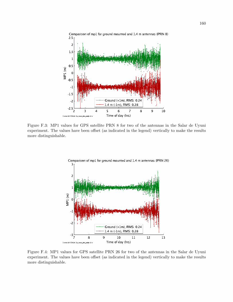
160

Figure F.3: MP1 values for GPS satellite PRN 8 for two of the antennas in the Salar de Uyuniexperiment. The values have been offset (as indicated in the legend) vertically to make the resultsmore distinguishable.

Figure F.4: MP1 values for GPS satellite PRN 26 for two of the antennas in the Salar de Uyuniexperiment. The values have been offset (as indicated in the legend) vertically to make the resultsmore distinguishable.

Documents

New Time and Multipath Augmentations for the Global