Embed Size (px)
Citation preview
1616 P St. NW Washington, DC 20036 202-328-5000 www.rff.org
June 2010
New U.S. Nuclear Generation: 2010–2030
Geof f re y Rothw e l l
BAC
KG
ROU
ND
ER

Contents
1. Executive Summary ............................................................................................................ 1
2. Current Status and Issues Regarding New Nuclear Generation .................................... 5
2.1: Changes in U.S. Nuclear Regulatory Commission Licensing Procedures .................. 6
2.2 The DOE Loan Guarantee Program for New Nuclear Generation ............................. 11
2.3 Pending U.S. Congressional Nuclear Power Legislation ............................................ 13
3. Modeling Nuclear Power Plant Construction and Levelized Costs ............................. 15
3.1. New Nuclear’s Capital-at-Risk: Total Capital Construction Cost ............................. 17
3.2 New Nuclear’s Levelized Cost per Megawatt-Hour ................................................... 19
3.3 Is the NEMS Estimate of New Nuclear’s “Overnight” Cost Reasonable? ................. 21
3.4 Risks and Uncertainties in New Nuclear Generation’s Costs ..................................... 23
3.5 A Review of Du and Parsons (2009) .......................................................................... 24
4. Expected New Nuclear Capacities in 2020 and 2030 ..................................................... 29
4.1 New Nuclear Capacity in NEMS-RFF under Base Case (Core_1) ............................ 30
4.2 New Nuclear Capacity in NEMS-RFF under Carbon Reduction (Core_2) ................ 31
4.3 Is the Estimate of Nuclear Capacity under Core_1 Reasonable? ............................... 33
4.5 Are These Experts Rational Regarding Additional Nuclear Capacity? ...................... 35
5. The Cost of Capital for New Nuclear Plant Owners in NEMS..................................... 39
5.1 Nuclear Generation’s Weighted Average Cost of Capital in NEMS .......................... 39
5.2 Lowering the Cost of Capital for Nuclear in NEMS-RFF .......................................... 43
6. Federal Financing of New Nuclear Generation, 2010–2020? ........................................ 48
6.1 Measuring the Influence of Federal Incentives on New Nuclear Generation ............. 48
6.2 Measuring the Cost of Federal Incentives to Encourage New Nuclear Generation ... 51
6.3 Measuring the Benefits of Federal Incentives for New Nuclear Generation .............. 54
7. Whither Irradiated Fuel? ................................................................................................. 57
7.1 Sequestering New Nuclear Power’s Used Fuel or Fossil Fuel’s CO2? ....................... 58
7.2 What are the Costs and Uncertainties of U.S. SNF Alternatives? .............................. 59
7.3 Is There Confidence in the “Waste Confidence Rule”? .............................................. 61

Abbreviations and Acronyms .............................................................................................. 66
References .............................................................................................................................. 68
Resources for the Future Rothwell
1
New U.S. Nuclear Generation: 2010–2030
Geoffrey Rothwell∗
1. Executive Summary
This report analyzes the modeling of the next generation of nuclear capacity in the National Energy Modeling System (NEMS), under the assumptions of the Energy Information Administration (EIA 2009a) authored by the Office of Integrated Analysis and Forecasting (OIAF; see http://www.eia.doe.gov/oiaf/brochures/oiafprod/) with modifications requested by Resources for the Future (RFF) to analyze the cases considered by research under the program, Toward a New National Energy Policy—Assessing the Options. This will be referred to as NEMS-RFF. The report’s key finding is that new nuclear capacity in NEMS-RFF from 2015 to 2020 under the current levels of U.S. Department of Energy (DOE) loan guarantees is similar to the marginal increase in new capacity from lowering the nominal return-on-equity (ROE) in NEMS-RFF for new nuclear power from 17 to 14 percent. This equivalence allows for an analysis of the costs and benefits of increasing DOE loan guarantees to new nuclear plants. In particular, based on these results, the present value of federal investment in new nuclear
∗ Geoffrey Rothwell, Department of Economics, Stanford University; [email protected]. This research was funded through Resources for the Future by the George Kaiser Family Foundation. I thank C. Braun, E. Brown, Y. Chang, M. Chu, G. Clement, T. Cochran, J. Conti, M. Corradini, M. Crozat, C. Forsberg, B. Fri, L. Goudarzi, L. Goulder, R. Graber, R. Hagen, K. Hayes, C. Heising, H. Huntington, G. Kaiser, H. Khalil, T. Knowles, B. Kong, D. Korn, A. Krupnik, G. Kulynych, W. Magwood, R. Matzie, A. MacFarlane, S. Mtingwa, G. Onopoko, K. Palmer, I. Parry, J. Parsons, S. Piet, T. Quinn, P. Peterson, W. Rasin, T. Retson, E. Schneider, S. Showalter, R. Versluis, K. Williams, T. Wood, and anonymous reviewers for their data, references, comments, and encouragement. These pages reflect the author’s views and conclusions and not those of any other organization or individual.
This background paper is one in a series developed as part of the Resources for the Future and National Energy Policy Institute project entitled “Toward a New National Energy Policy: Assessing the Options.” This project was made possible through the support of the George Kaiser Family Foundation.
© 2010 Resources for the Future. All rights reserved. No portion of this paper may be reproduced without permission of the authors.
Background papers are research materials circulated by their authors for purposes of information and discussion. They have not necessarily undergone formal peer review.
Resources for the Future Rothwell
2
generation can reduce carbon dioxide emissions (CO2) for less than $2/tonne, which is less than most alternatives.
Section 2 of this report introduces the current status of new nuclear capacity in the United States. Section 3 discusses the cost of this capacity. Section 4 presents base case results of NEMS-RFF scenarios known as Core_1, Obama CAFE Target; Core_2, Cap-and-Trade with a Two Billion Ton Limit on Offsets; and Core_2n, Cap-and-Trade with a One Billion Ton Limit on Offsets.
Section 5 analyzes the results of two variations of Core_1: (a) Core_1_14%, where the rate of Return-on-Equity is lowered from the OIAF’s assumed 17 percent (nominal) to 14 percent (nominal), and (b) Core_1_11%, where ROE is lowered to 11 percent (nominal). Core_1 results are subtracted from Core_1_14% and Core_1_11%; these results are referred to as ROE_14% and ROE_11%. In Core_1_14% , a Weighted Average Cost of Capital of 10 percent nominal (with a 14 percent nominal Return-on-Equity) reduces the levelized unit electricity cost and increases the construction of new nuclear capacity from 12.7 gigawatts (GW) in 2020 to 57 GW in 2030. In Core_1_11%, a Weighted Average Cost of Capital of 8.25 percent nominal (with an 11 percent nominal Return-on-Equity) reduces the levelized cost even further and leads to a boom in new nuclear capacity from 23.5 GW in 2020 to 136 GW in 2030 in NEMS-RFF.
Section 6 focuses on the costs and benefits of increasing DOE loan guarantees between 2010 and 2020 under the assumption that federal incentives will not be required after 2020 (with an effective carbon control mechanism). To understand the influence of loan guarantees, compare the results of the Core_1 variants:
• Core_1 projects 6.2 GW (under the influence of current incentives), and
• ROE_14% projects an additional 6.5 GW for a total of 12.7 GW, or
• ROE_11% projects an additional 17.3 GW for a total of 23.5 GW by 2020.
The influence of the Energy Policy Act of 2005 and subsequent appropriations bills (EPAct05+) incentives (yielding 6.2 GW in new nuclear capacity) is similar to lowering the Return-on-Equity in for nuclear investors to 14 percent (yielding a similar additional 6.5 GW of nuclear capacity): If DOE were to double the size of the Loan Guarantee Program, new Generation III capacity should be similar to that under Core_1_14%—that is, around 12 GW. If DOE were to expand the program further, new nuclear capacity could be even greater by 2020.
Resources for the Future Rothwell
3
What would be the cost to taxpayers of the equivalent of reducing the Weighted Average Cost of Capital to 10 percent (or further to 8.25 percent) for other nuclear power plant investors, which could induce the construction of another 6.5 GW (or another 17.3 GW) by 2020?
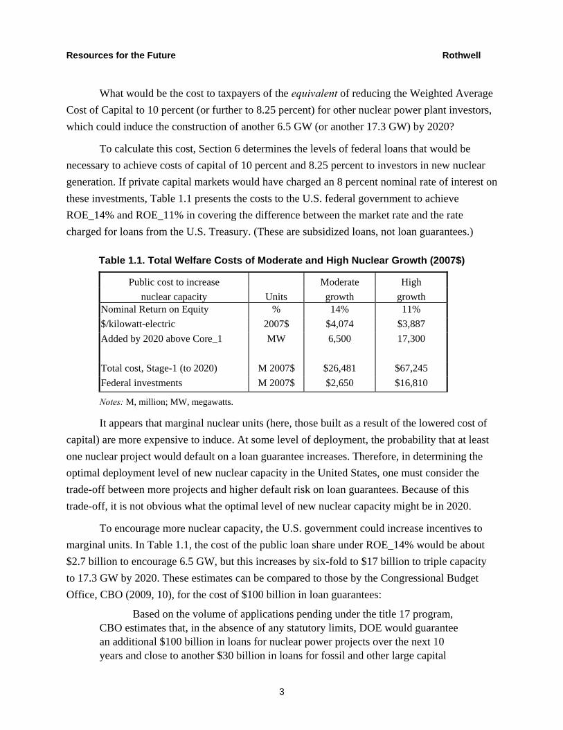
To calculate this cost, Section 6 determines the levels of federal loans that would be necessary to achieve costs of capital of 10 percent and 8.25 percent to investors in new nuclear generation. If private capital markets would have charged an 8 percent nominal rate of interest on these investments, Table 1.1 presents the costs to the U.S. federal government to achieve ROE_14% and ROE_11% in covering the difference between the market rate and the rate charged for loans from the U.S. Treasury. (These are subsidized loans, not loan guarantees.)
Table 1.1. Total Welfare Costs of Moderate and High Nuclear Growth (2007$)
Public cost to increase Moderate High nuclear capacity Units growth growth
Nominal Return on Equity % 14% 11% $/kilowatt-electric 2007$ $4,074 $3,887 Added by 2020 above Core_1 MW 6,500 17,300 Total cost, Stage-1 (to 2020) M 2007$ $26,481 $67,245 Federal investments M 2007$ $2,650 $16,810
Notes: M, million; MW, megawatts.
It appears that marginal nuclear units (here, those built as a result of the lowered cost of capital) are more expensive to induce. At some level of deployment, the probability that at least one nuclear project would default on a loan guarantee increases. Therefore, in determining the optimal deployment level of new nuclear capacity in the United States, one must consider the trade-off between more projects and higher default risk on loan guarantees. Because of this trade-off, it is not obvious what the optimal level of new nuclear capacity might be in 2020.
To encourage more nuclear capacity, the U.S. government could increase incentives to marginal units. In Table 1.1, the cost of the public loan share under ROE_14% would be about $2.7 billion to encourage 6.5 GW, but this increases by six-fold to $17 billion to triple capacity to 17.3 GW by 2020. These estimates can be compared to those by the Congressional Budget Office, CBO (2009, 10), for the cost of $100 billion in loan guarantees:
Based on the volume of applications pending under the title 17 program, CBO estimates that, in the absence of any statutory limits, DOE would guarantee an additional $100 billion in loans for nuclear power projects over the next 10 years and close to another $30 billion in loans for fossil and other large capital
Resources for the Future Rothwell
4
projects. We expect that fees paid by borrowers would be at least 1 percent lower than the amount needed to cover the costs of the guarantee; consequently, the legislation would increase spending for credit subsidies by $1 billion over the next 10 years.
Thus, the estimates here of between $2.7 billion and $17 billion should be considered to be at the very high end of a possible range of costs to the U.S. government to encourage carbon-free nuclear generation.
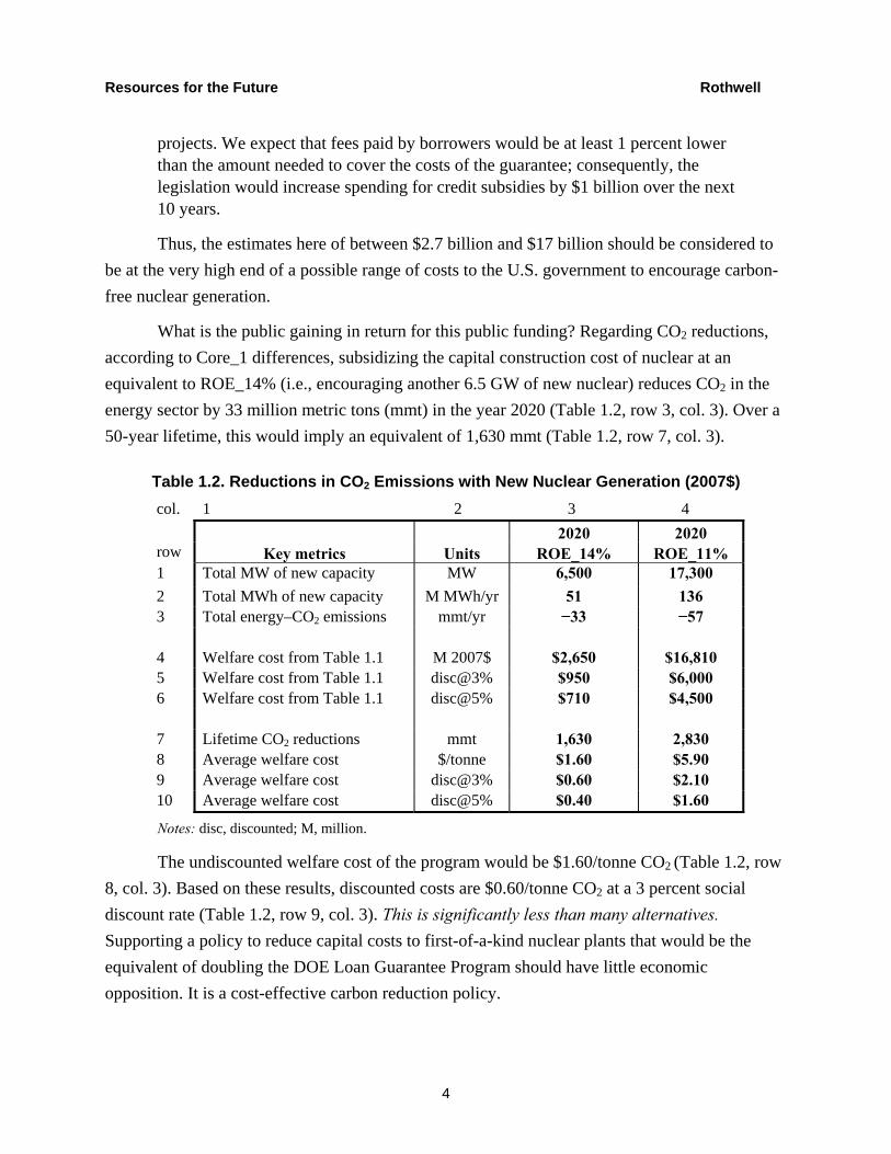
What is the public gaining in return for this public funding? Regarding CO2 reductions, according to Core_1 differences, subsidizing the capital construction cost of nuclear at an equivalent to ROE_14% (i.e., encouraging another 6.5 GW of new nuclear) reduces CO2 in the energy sector by 33 million metric tons (mmt) in the year 2020 (Table 1.2, row 3, col. 3). Over a 50-year lifetime, this would imply an equivalent of 1,630 mmt (Table 1.2, row 7, col. 3).
Table 1.2. Reductions in CO2 Emissions with New Nuclear Generation (2007$) col. 1 2 3 4
Key metrics Units 2020 2020
row ROE_14% ROE_11% 1 Total MW of new capacity MW 6,500 17,300 2 Total MWh of new capacity M MWh/yr 51 136 3 Total energy–CO2 emissions mmt/yr −33 −57 4 Welfare cost from Table 1.1 M 2007$ $2,650 $16,810 5 Welfare cost from Table 1.1 disc@3% $950 $6,000 6 Welfare cost from Table 1.1 disc@5% $710 $4,500 7 Lifetime CO2 reductions mmt 1,630 2,830 8 Average welfare cost $/tonne $1.60 $5.90 9 Average welfare cost disc@3% $0.60 $2.10 10 Average welfare cost disc@5% $0.40 $1.60
Notes: disc, discounted; M, million.
The undiscounted welfare cost of the program would be $1.60/tonne CO2 (Table 1.2, row 8, col. 3). Based on these results, discounted costs are $0.60/tonne CO2 at a 3 percent social discount rate (Table 1.2, row 9, col. 3). This is significantly less than many alternatives. Supporting a policy to reduce capital costs to first-of-a-kind nuclear plants that would be the equivalent of doubling the DOE Loan Guarantee Program should have little economic opposition. It is a cost-effective carbon reduction policy.
Resources for the Future Rothwell
5
Subsidizing the capital construction cost of nuclear (Core_1_11%) to encourage an additional 17.3 GW of new nuclear by 2020 reduces CO2 in the energy sector by 57 mmt per year in the year 2020 according to NEMS-RFF (Table 1.2, row 3, col. 4). Over a 50-year lifetime, this would imply an equivalent of 2,830 mmt (Table 1.2, row 7, col. 4.) Based on NEMS-RFF results, the undiscounted welfare cost of the program would be $5.90/tonne CO2 (Table 1.2, row 8, col. 4). The discount cost is $2.10/tonne CO2 at a 3 percent social discount rate (Table 1.2, row 9, col. 4). (These values would be much lower under the CBO analysis.)
Doubling the Loan Guarantee Program yields results in NEMS-RFF that are similar to those obtained by lowering the Return-on-Equity to 14 percent. However, because of discontinuities in NEMS-RFF projections (see the year 2021 in Table 5.4) and the complexities in modeling the Loan Guarantee Program in NEMS, it is difficult to determine the optimal level of loan guarantees without further analysis.
Unlike other studies on the future of nuclear generation in the United States, this study can be easily extended to satisfy the requirement of a NEMS analysis of congressional legislation (e.g., the American Power Act [APA]). An analysis of the American Clean Energy and Security Act (ACESA; H.R. 2454) was done in OIAF (2009). This report can be updated to analyze current policy proposals by running the NEMS base case with Returns-on-Equity of 14 percent, 13 percent, 12 percent, and 11 percent for financing new nuclear power plants. Costs can be calculated as done in Table 1.1, and CO2-reduction benefits and the average welfare cost of these CO2 reductions can be calculated as in Table 1.2.
Given the results here, the most cost-effective alternative would be equivalent to a subsidized Return-on-Equity to nuclear investors below 14 percent (nominal), which has been shown to be equivalent to at least doubling the DOE Loan Guarantee Program targeting new nuclear capacity. However, these results assume that the new nuclear power plant licensing procedures, described in the next section, work smoothly and expeditiously.
2. Current Status and Issues Regarding New Nuclear Generation
The last nuclear power plant ordered, and not subsequently cancelled, was Palo Verde in Arizona in October 1973. After the oil embargo, starting that month, the growth in electricity demand dropped from about 7 percent per year to about 3 percent per year throughout the 1970s, leading to delays in the construction of many nuclear plants. Later in the 1970s, with double-digit inflation and associated increases in the cost of capital approaching 20 percent, capital-intensive nuclear plants were cancelled. Further, after the accident at Three Mile Island on March
Resources for the Future Rothwell
6
28, 1979, the costs of constructing nuclear plants and the time to license them doubled, leading to more nuclear power plant cancellations. The last nuclear power plant placed in service in the United States was Watts Bar in 1996 (where construction began in 1973). It is also at Watts Bar where nuclear construction has restarted with the Tennessee Valley Authority’s decision to complete Unit 2.
In response to the problems facing the nuclear power industry during the last two decades, Congresses and administrations have attempted to reenergize nuclear generation. The remainder of this section summarizes recent changes in regulation and legislation. Section 7 discusses the issue of irradiated fuel management.
2.1: Changes in U.S. Nuclear Regulatory Commission Licensing Procedures
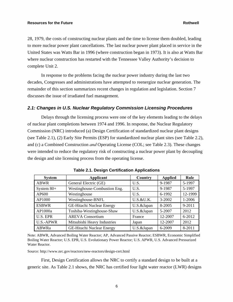
Delays through the licensing process were one of the key elements leading to the delays of nuclear plant completions between 1974 and 1996. In response, the Nuclear Regulatory Commission (NRC) introduced (a) Design Certification of standardized nuclear plant designs (see Table 2.1), (2) Early Site Permits (ESP) for standardized nuclear plant sites (see Table 2.2), and (c) a Combined Construction and Operating License (COL; see Table 2.3). These changes were intended to reduce the regulatory risk of constructing a nuclear power plant by decoupling the design and site licensing process from the operating license.
Table 2.1. Design Certification Applications
System Applicant Country Applied Rule ABWR General Electric (GE) U.S. 9-1987 5-1997 System 80+ Westinghouse-Combustion Eng. U.S. 9-1987 5-1997 AP600 Westinghouse U.S. 6-1992 12-1999AP1000 Westinghouse-BNFL U.S.&U.K. 3-2002 1-2006 ESBWR GE-Hitachi Nuclear Energy U.S.&Japan 8-2005 9-2011 AP1000a Toshiba-Westinghouse-Shaw U.S.&Japan 5-2007 2012 U.S. EPR AREVA Consortium France 12-2007 6-2012 U.S.-APWR Mitsubishi Heavy Industries Japan 12-2007 2012 ABWRa GE-Hitachi Nuclear Energy U.S.&Japan 6-2009 8-2011
Note: ABWR, Advanced Boiling Water Reactor; AP, Advanced Passive Reactor; ESBWR, Economic Simplified Boiling Water Reactor; U.S. EPR, U.S. Evolutionary Power Reactor; U.S. APWR, U.S. Advanced Pressurized Water Reactor.
Source: http://www.nrc.gov/reactors/new-reactors/design-cert.html
First, Design Certification allows the NRC to certify a standard design to be built at a generic site. As Table 2.1 shows, the NRC has certified four light water reactor (LWR) designs

Resources for the Future Rothwell
7
and has five designs (or amendments to designs) under active review: the Advanced Boiling Water Reactor (ABWR, amended), the Advanced Passive reactor (AP1000a, amended), the Economic Simplified Boiling Water Reactor (ESBWR), the US Evolutionary Power Reactor (U.S. EPR), and the U.S. Advanced Pressurized Water Reactor (US-APWR). There is no longer interest in constructing any of the designs that have already been licensed. However, there is great interest in an amended AP1000 design, the AP1000a, which is expected to have its Final Safety Evaluation Report approved before 2012. Then the NRC must approve the Design Certification (in a final ruling), which could add 6 to 12 months to the approval process. So it is unlikely that construction of proposed plants will start before 2012 or finish before the end of 2018.
Second, the ESP process allows a nuclear investor to license a specific site for a generic LWR with the option of constructing a plant within 10 to 20 years, as well as renewing it for an additional 10 to 20 years. Only four sites have been approved: Clinton in Illinois, Grand Gulf in Mississippi, North Anna in Virginia, and Vogtle in Georgia. (The Vogtle plant is in bold in all Section 2 tables because it has received and accepted an offer of a large DOE loan guarantee of $8.33 billion, and therefore can be considered a standard by which to evaluate other projects.)
Table 2.2. ESP Applications
Proposed new reactor(s) County, State
Submit date
Approval date
Clinton DeWitt, IL Sep-03 Mar-07
Grand Gulf Claiborne, MS, Oct-03 Apr-07
North Anna Louisa, VA Sep-03 Nov-07
Vogtle Burke, GA Aug-06 Aug-09
Victoria County Victoria, TX Mar-10 Unknown Source: http://www.nrc.gov/reactors/new-reactors/esp.html
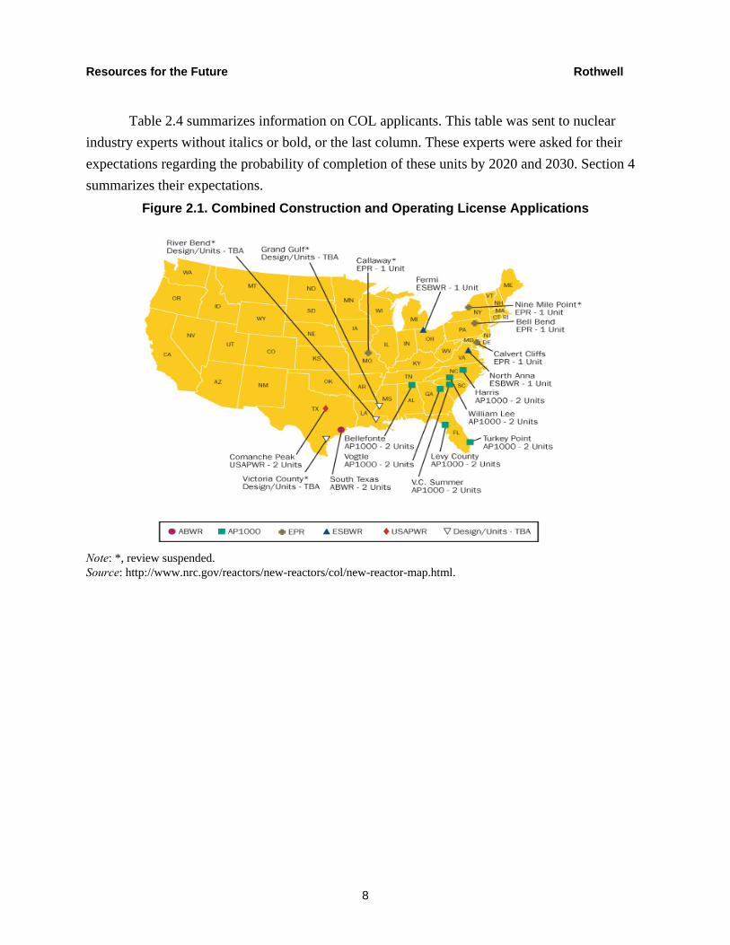
Third, in 1989, the NRC introduced a new licensing procedure that would allow for the issuance of a COL so the nuclear plant owner could be assured of commercial operation by demonstrating that the plant met all initially agreed upon criteria for operation at the completion of construction. The first COL application was submitted for two units at the South Texas Project on November 29, 2007, with an estimated commercialization date near 2017 (see Rothwell 2006). Since then, the nuclear utility industry has applied for more than two dozen COLs (Figure 2.1 and Table 2.3).
Resources for the Future Rothwell
8
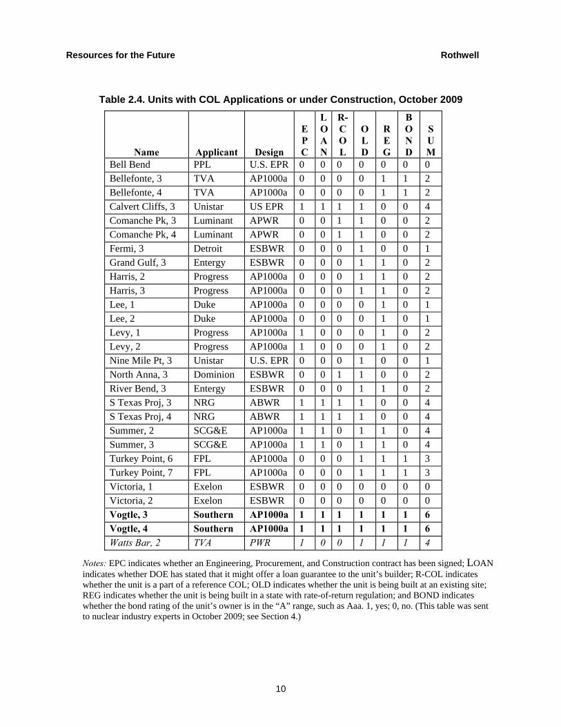
Table 2.4 summarizes information on COL applicants. This table was sent to nuclear industry experts without italics or bold, or the last column. These experts were asked for their expectations regarding the probability of completion of these units by 2020 and 2030. Section 4 summarizes their expectations.
Figure 2.1. Combined Construction and Operating License Applications
Note: *, review suspended. Source: http://www.nrc.gov/reactors/new-reactors/col/new-reactor-map.html.
Resources for the Future Rothwell
9
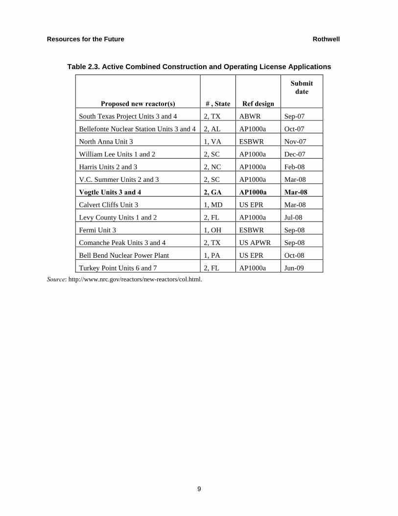
Table 2.3. Active Combined Construction and Operating License Applications
Proposed new reactor(s) # , State Ref design
Submit date
South Texas Project Units 3 and 4 2, TX ABWR Sep-07
Bellefonte Nuclear Station Units 3 and 4 2, AL AP1000a Oct-07
North Anna Unit 3 1, VA ESBWR Nov-07
William Lee Units 1 and 2 2, SC AP1000a Dec-07
Harris Units 2 and 3 2, NC AP1000a Feb-08
V.C. Summer Units 2 and 3 2, SC AP1000a Mar-08
Vogtle Units 3 and 4 2, GA AP1000a Mar-08
Calvert Cliffs Unit 3 1, MD US EPR Mar-08
Levy County Units 1 and 2 2, FL AP1000a Jul-08
Fermi Unit 3 1, OH ESBWR Sep-08
Comanche Peak Units 3 and 4 2, TX US APWR Sep-08
Bell Bend Nuclear Power Plant 1, PA US EPR Oct-08
Turkey Point Units 6 and 7 2, FL AP1000a Jun-09 Source: http://www.nrc.gov/reactors/new-reactors/col.html.
Resources for the Future Rothwell
10
Table 2.4. Units with COL Applications or under Construction, October 2009
Name Applicant Design
EPC
LOAN
R-COL
OLD
REG
BOND
SUM
Bell Bend PPL U.S. EPR 0 0 0 0 0 0 0 Bellefonte, 3 TVA AP1000a 0 0 0 0 1 1 2 Bellefonte, 4 TVA AP1000a 0 0 0 0 1 1 2 Calvert Cliffs, 3 Unistar US EPR 1 1 1 1 0 0 4 Comanche Pk, 3 Luminant APWR 0 0 1 1 0 0 2 Comanche Pk, 4 Luminant APWR 0 0 1 1 0 0 2 Fermi, 3 Detroit ESBWR 0 0 0 1 0 0 1 Grand Gulf, 3 Entergy ESBWR 0 0 0 1 1 0 2 Harris, 2 Progress AP1000a 0 0 0 1 1 0 2 Harris, 3 Progress AP1000a 0 0 0 1 1 0 2 Lee, 1 Duke AP1000a 0 0 0 0 1 0 1 Lee, 2 Duke AP1000a 0 0 0 0 1 0 1 Levy, 1 Progress AP1000a 1 0 0 0 1 0 2 Levy, 2 Progress AP1000a 1 0 0 0 1 0 2 Nine Mile Pt, 3 Unistar U.S. EPR 0 0 0 1 0 0 1 North Anna, 3 Dominion ESBWR 0 0 1 1 0 0 2 River Bend, 3 Entergy ESBWR 0 0 0 1 1 0 2 S Texas Proj, 3 NRG ABWR 1 1 1 1 0 0 4 S Texas Proj, 4 NRG ABWR 1 1 1 1 0 0 4 Summer, 2 SCG&E AP1000a 1 1 0 1 1 0 4 Summer, 3 SCG&E AP1000a 1 1 0 1 1 0 4 Turkey Point, 6 FPL AP1000a 0 0 0 1 1 1 3 Turkey Point, 7 FPL AP1000a 0 0 0 1 1 1 3 Victoria, 1 Exelon ESBWR 0 0 0 0 0 0 0 Victoria, 2 Exelon ESBWR 0 0 0 0 0 0 0 Vogtle, 3 Southern AP1000a 1 1 1 1 1 1 6 Vogtle, 4 Southern AP1000a 1 1 1 1 1 1 6 Watts Bar, 2 TVA PWR 1 0 0 1 1 1 4
Notes: EPC indicates whether an Engineering, Procurement, and Construction contract has been signed; LOAN indicates whether DOE has stated that it might offer a loan guarantee to the unit’s builder; R-COL indicates whether the unit is a part of a reference COL; OLD indicates whether the unit is being built at an existing site; REG indicates whether the unit is being built in a state with rate-of-return regulation; and BOND indicates whether the bond rating of the unit’s owner is in the “A” range, such as Aaa. 1, yes; 0, no. (This table was sent to nuclear industry experts in October 2009; see Section 4.)
Resources for the Future Rothwell
11
2.2 The DOE Loan Guarantee Program for New Nuclear Generation
DOE has started a series of programs to provide incentives to new nuclear generators, including the Nuclear Power 2010 (NP2010) Program. This program envisioned having a new nuclear plant operating in the United States by 2010: “The conclusions and recommendations provide important information for all decision-makers involved in the goal of operating a new nuclear plant by 2010” (Crosbie and Kidwell 2004, iv). Several feasibility studies were funded, including one for the construction of two units at the South Texas Project. However, few plants were ordered until the passage of EPAct05, which recognized that a major obstacle to nuclear plant orders was access to capital. The most important provision of EPAct05 was the Loan Guarantee Program, which was intended to reimburse investors for the potential loss of their capital and interest in constructing nuclear power plants. But no funds were allocated for this program until later appropriations bills.
Three provisions in EPAct05 promote nuclear capacity. Two of these programs—Production Tax Credits and Standby Support—have benefits that are dispensed disproportionately to early qualifying nuclear plants, primarily the first half-dozen units. To be eligible for these programs, the COL application filing deadline was December 31, 2008 (see Table 2.3). Production Tax Credits and Standby Support Programs are discussed in Rothwell and Graber (2008).
Whereas the Production Tax Credit Program is intended to subsidize nuclear operations (through tax reductions) and the Standby Support Program is meant to stabilize the new nuclear licensing process, the DOE Loan Guarantee Program is intended to promote carbon-free emissions in electricity production from low-carbon energy technologies, including nuclear capacity. EPAct05 Title XVII states that advanced nuclear plants are eligible for loan guarantees (although it did not specify an amount). This has particular significance for the nuclear industry because of the 1970s default of $2.25 billion of municipal debt by the Washington Public Power Supply System for the construction of nuclear power plants in Washington State—at that time the largest municipal bond default in U.S. history.
As clarified in DOE (2007) the Loan Guarantee Program covers up to 100 percent of the loan cost with the limitation that the guaranteed loans compose no more than 80 percent of the total project cost. The program provides for the repayment of principal and interest on the loan should the borrower default. In the event of a default, the developer may be required to reimburse the U.S. Treasury for the amount of the defaulted loan after the U.S. Attorney General
Resources for the Future Rothwell
12
recovers any value in the assets. With a maximum of 80 percent of the project guaranteed, the remainder of the project cost must be covered by equity investors.
EPAct05 plus the appropriations bills, EPAct05+, established the amount of the Loan Guarantee Program for nuclear generation at $18.5 billion, to be administered by DOE. But DOE must limit the funding to applicants to spread the $18.5 billion over more than one design. Without this limit, only a few nuclear units would be likely to receive loan guarantees because the cost of these first-of-a-kind nuclear power plants is likely to exceed $5 billion per 1,000 MW of nuclear capacity (including Interest During Construction, IDC, and escalation). The DOE Loan Guarantee Program is discussed in Sections 5 and 6.
Although the selection of plants has not been finalized and the terms of the agreements completed, Vogtle with Southern in Georgia has been offered and accepted a loan guarantee of $8.33 billion and three other plants have been given positive initial reviews from DOE: South Texas with the company NRG in Texas, Summer with South Carolina Electric & Gas (SCE&G), and Calvert Cliffs with Unistar in Maryland. Also, Comanche Peak with Luminant in Texas is considered an alternative to any of the four projects should one of these applicants withdraw from the Loan Guarantee Program. According to the White House’s Office of the Press Secretary (2010), “Underscoring his Administration’s commitment to jumpstarting the nation’s nuclear generation industry, President Obama today announced that the Department of Energy has offered conditional commitments for a total of $8.33 billion in loan guarantees for the construction and operation of two new nuclear reactors at a plant in Burke, Georgia [Vogtle].”
Even with loan guarantees, the builders of these nuclear power plants will have to convince Wall Street in times of capital constraints that investing in nuclear generation does not involve more risk than similar investments. However, Moody’s (2009) wrote (updating Moody’s 2007 and 2008),
Moody’s is considering taking a more negative view for those issuers seeking to build new nuclear power plants. [This] is premised on a material increase in business and operating risk. Their longer-term [net present value appears positive], and, once operating, nuclear plants are viewed favorably due to their economics and no-carbon emission footprint. Historically, most nuclear-building utilities suffered ratings downgrades—and sometimes several—while building these facilities. Most utilities now seeking to build nuclear generation do not appear to be adjusting their financial policies, [leading to] a credit [rating downgrade]. First federal approvals are at least two years away, and economic, political and policy equations could easily change before then. Progress continues slowly on Federal Loan Guarantees, which will provide a lower-cost source of

Resources for the Future Rothwell
13
funding, but will only modestly mitigate increasing business and operating risk profiles. Partnerships, balance sheet strengthening, bolstering liquidity reserves, and ‘back-to-basics’ approaches to core operations could help would-be nuclear utilities maintain their [credit] ratings. (emphasis added)
2.3 Pending U.S. Congressional Nuclear Power Legislation
On June 26, 2009, the U.S. House of Representatives passed ACESA (H.R. 2454), also known as the Waxman–Markey bill after its authors, Henry Waxman (D-CA) and Edward Markey (D-MA). The bill ignores nuclear power generation, but (a) introduces a cap-and-trade program to reduce carbon emissions and (b) creates the Clean Energy Deployment Administration (CEDA) to administer loan guarantee programs for advanced energy technologies.
An analysis of ACESA’s impacts on the U.S. energy economy (particularly of the carbon control program, similar to Core_2, discussed in Section 4) was performed by OIAF with NEMS (see OIAF 2009). That report finds little deployment of nuclear capacity by 2020 and further limits nuclear capacity because: “There is great uncertainty about how fast these technologies, the industries that support them, and the regulatory infrastructure that licenses/permits them might be able to grow and, for fossil with [carbon capture and sequestration, CCS], when the technology will be fully commercialized. For nuclear, this assumption limits new plant additions to roughly 11,000 megawatts, or 7 to 11 new generators, by 2030” (OIAF 2009, 6). As discussed in Sections 4–6, these are roughly equivalent to Core_1 results. Further, “The Reference Case projects 11 gigawatts of new nuclear capacity by 2030, but under ACESA, nuclear builds by 2030 range from 15 gigawatts to 135 gigawatts, when allowed to grow.” (OIAF 2009, 20, emphasis added)
On July 16, 2009, Senator Jeff Bingaman (D-NM) introduced a similar Senate bill, the American Clean Energy Leadership Act of 2009 (S. 1462). One of the primary differences between the two bills was that, under S. 1462, no congressional appropriation would be required for loan guarantees through CEDA. This could lead to large loan guarantees to the nuclear industry, as pointed out in CBO’s (2009, 9–10) cost analysis of S. 1462:
Modifications to DOE’s Title 17 Loan Guarantee Program. S. 1462 would modify the terms of DOE’s Loan Guarantee program for advanced energy technologies, which was established under title 17 of the Energy Policy Act of 2005. The bill would exempt the title 17 program from the provisions in FCRA [Federal Credit Reform Act of 1990] that require such programs to receive an appropriation. The effect of this exemption would be to give DOE permanent
Resources for the Future Rothwell
14
authority to guarantee such loans without further legislative action or limitations. . . . CBO estimates that enacting those changes would increase spending by $1.8 billion over the 2010–2019 period. . . .
Based on financial information about costly energy investments, such as nuclear power plants, CBO estimates that the premiums charged to borrowers will, on average, be at least 1 percent lower than the likely cost of the guarantees. Based on the volume of applications pending under the title 17 program, CBO estimates that, in the absence of any statutory limits, DOE would guarantee an additional $100 billion in loans for nuclear power projects over the next 10 years and close to another $30 billion in loans for fossil and other large capital projects. We expect that fees paid by borrowers would be at least 1 percent lower than the amount needed to cover the costs of the guarantee; consequently, the legislation would increase spending for credit subsidies by $1 billion over the next 10 years.
However, S. 1462 did not reach the Senate floor. Instead, on May 12, 2010, Senators John Kerry (D-MA) and Joe Lieberman (I-CT) introduced the “American Power Act” (APA). Unlike H.R. 2454 or S. 1462, the APA (§1001) begins with a nuclear-positive policy statement:
TITLE I–DOMESTIC CLEAN ENERGY DEVELOPMENT, Subtitle A–Nuclear Power, SEC. 1001. STATEMENT OF POLICY. It is the policy of the United States, given the importance of transitioning to a clean energy, low-carbon economy, to facilitate the continued development and growth of a safe and clean nuclear energy industry, through (1) reductions in financial and technical barriers to construction and operation; and (2) incentives for the growth of safe domestic nuclear and nuclear-related industries.
To grow the nuclear energy industry, in Section 1102, the APA increases the Title 17 Loan Guarantee Program from $47 billion to $100 billion and increases the DOE Loan Guarantee Program from $18.5 billion to $54 billion (as proposed by the Obama administration; Wald 2010). Other incentives for nuclear energy in the APA are intended to (a) include more nuclear plants in the Standby Support Program; (b) support research and development (R&D) in spent fuel recycling, in reducing costs of nuclear power generation, and in small reactors; and (c) encourage investment in new nuclear power plants, particularly with regard to tax provisions (Title 1-Part III, accelerated depreciation and investment tax credits). Because the APA was introduced so late in the 111th Congress, it is unlikely that differences between the House’s ACESA and the Senate’s APA will be resolved before the 2010 congressional elections. Thus, the issue of the appropriate level of loan guarantees may be debated throughout the next Congress.
Resources for the Future Rothwell
15
To discover whether there is an optimal level of loan guarantees, Section 3 discusses the expected costs of new nuclear capacity. Section 4 explores whether NEMS estimates of new nuclear capacity are reasonable. Section 5 examines the cost of capital facing nuclear power plant investors and what incentives might be needed to increase nuclear capacity. Section 6 concludes that the analysis here supports increasing the DOE Loan Guarantee Program based on the value of reducing CO2. Section 7 discusses policy issues associated with used fuel.
3. Modeling Nuclear Power Plant Construction and Levelized Costs
Although the impact of each of the incentives outlined in Section 2 could be analyzed separately, Rothwell and Graber (2008) find that only loan guarantees encourage new nuclear plant orders (in the absence of carbon fees). To understand the importance of loan guarantees on the decision to build new nuclear capacity, this section reviews the costs and financing of constructing new nuclear power plants following the cost-estimating standards of the Economic Modeling Working Group (EMWG 2007). This section addresses whether construction costs assumed by OIAF in NEMS are reasonable (see EIA 2009a).
One can measure nuclear capacity competitiveness in three ways: (a) Capital-at-Risk, (b) levelized unit electricity cost (LUEC) or average cost (AC), and (c) net present value (NPV). Because NEMS does not calculate NPV, it will not be discussed further. (For simulations of stochastic NPVs for ABWRs at the South Texas Project, see Rothwell 2006.) Under rate-of-return regulation, and in NEMS, the comparison of LUEC dominates decision making. But in deregulated markets, Capital-at-Risk becomes important as the ratio of the nuclear investor’s Capital-at-Risk grows relative to the nuclear investor’s assets. How does NEMS calculate Capital-at-Risk and LUEC?
First, Capital-at-Risk is the total amount spent on construction and testing before any electricity or revenues are generated. In NEMS, Capital-at-Risk is measured by the total capital construction cost (TCC). As shown in Section 3.1, TCC is equal to total overnight construction cost (TOC) plus financing costs. In NEMS, TOC is $3,318/kilowatt (kW) in 2007$ (EIA 2009a, Table 8.2). If the real cost of capital is 10 percent and the construction duration is 72 months, as assumed in NEMS, the financing costs would be about 34.2 percent of TOC, or about $1,135/kW. So TCC for “advanced nuclear” in NEMS would be about $4,450/kW. The capital-at-risk (not including the first fuel load) would be about $6 billion for a 1,350-MW power plant in 2007$.
Resources for the Future Rothwell
16
The second key metric of nuclear competitiveness in NEMS is the plant’s LUEC, which is equivalent to (long-run) AC in microeconomics. The LUEC is defined by the Organisation for Economic Co-operation and Development in International Energy Agency/Nuclear Energy Agency (1998) as
T T
AC = Σ [{CRF · TCC + O&Mt + FUELt} (1 + R)-t] / Σ [E t (1 + R)-t] (3.1)
t =1 t =1
where
• [CRF(R,T) · TCC ] is the annual capital expenditure in each period, CRF is the Capital Recovery Factor, which is a function of the annual discount rate, R, and the economic life of the plant in years, T: {R (1 + R)T / [(1 + R)T – 1]};
• O&Mt are the annual operations and maintenance expenditures, including salaries and benefits in period t;
• FUELt is the annual fuel expenditure in period t; and
• Et is the annual production of electricity in megawatt-hours (MWh) in period t. For example, if the size of the plant is 1,350 MW (from EIA 2009a, Table 8.2) and the capacity factor is 90 percent, then the plant could produce about 10.65 million MWh per year.
If, after construction, annual expenditures and production are constant, then
AC = [(CRF · TCC + O&M + FUEL) · Σ (1 + R)-t] / E · Σ [(1 + R)-t]
= [(CRF · TCC + O&M + FUEL)] / E
= [CRF · TCC / E ] + O&M_MWh + FUEL_MWh (3.2)
where O&M_MWh and FUEL_MWh are variable costs for new nuclear generation.
For example, if (a) TCC were $6,000 million, (b) the discount rate were 10 percent real, (c) the lifetime were 50 years, (d) the output were 10.65 million MWh, (e) O&M_MWh were $10/MWh, and (f) FUEL_MWh were $10/MWh, then AC would be about $77/MWh (in 2007$; e.g., see Table 3.3). The remainder of Section 3 explores each of these cost metrics, whether NEMS uses reasonable cost estimates, and the influence of uncertainties associated with each metric on potential nuclear power plant builders.

Resources for the Future Rothwell
17
3.1. New Nuclear’s Capital-at-Risk: Total Capital Construction Cost
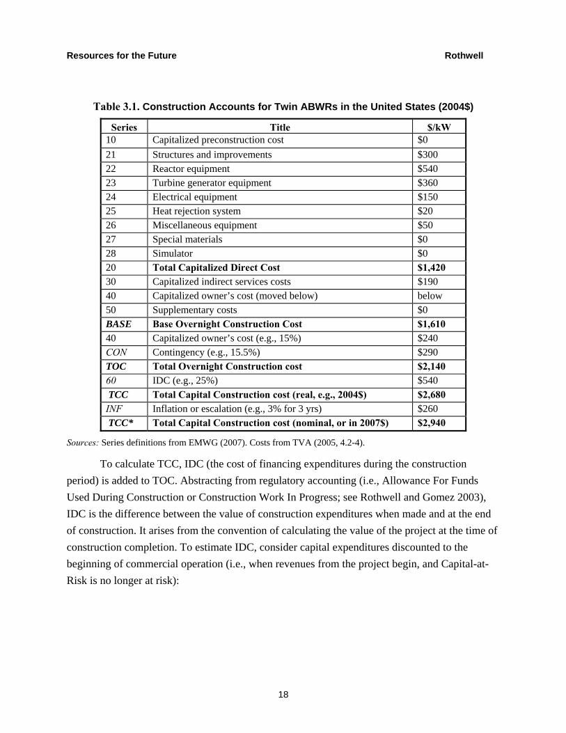
Table 3.1 presents the construction cost accounts for a nuclear power plant, based on the EMWG code of accounts (defining sets, known as “series,” of related costs) from EMWG (2007) with cost data from TVA (2005), which estimated costs for building a dual-unit ABWR; the costs are in dollars per kilowatt. Series 10 includes expenditures before construction, such as site purchase and licensing. Series 20 includes all items normally associated with the construction of a steam-electric generating station. Series 30 accounts for indirect costs, such as engineering and administration that cannot be associated with a specific cost category in Series 20. Series 40 includes all costs incurred by the owner associated with the plant and plant site. Series 50 includes supplemental costs, such as the first fuel core costs. (Nuclear fuel cost accounting is complex because of the different stages and stage durations of this asset during its perpetual life.)
The sum of Series 10 to 50 is the base overnight construction cost, or BASE. (The term overnight is used to describe what it would cost if money had no time value.) To this is added contingency, CON. BASE plus CON equals TOC. TOC plus Series 60, IDC, is TCC, which is the consensus measure of Capital-at-Risk in EMWG (2007). TCC is expressed in real dollars (e.g., 2007$), whereas TCC* is the sum of nominal dollars over several years (e.g., inflating at 3 percent per year).
This accounting system can be applied to NEMS: EIA (2009a, Table 8.2) states that the base overnight construction cost in 2008 (2007$/kW) for “advanced nuclear” is $2,873—in other words, the sum of Series 10, 20, 30, 40, and 50 in Table 3.1. Two types of contingency factors are included: a project contingency factor of 10 percent and a technological optimism factor of 5 percent. (In the notes to Table 8.2, EIA 2009a indicates “[a] contingency allowance is defined by the American Association of Cost Engineers [sic, name changed, see Association for the Advancement of Cost Engineering International 1997] as the ‘specific provision for unforeseeable elements [of] costs with a defined project scope’.” Also, “[t]he technological optimism factor is applied to the first four units of a new, unproven design. It reflects the demonstrated tendency to underestimate actual costs for a first-of-a-kind unit.”) Thus, the contingency multiplier is (1.1 x 1.05) = 1.155. The TOC (in 2007$) is ($2,873 x 1.155) = $3,318/kW in NEMS. Is this reasonable?
Resources for the Future Rothwell
18
Table 3.1. Construction Accounts for Twin ABWRs in the United States (2004$)
Series Title $/kW 10 Capitalized preconstruction cost $0 21 Structures and improvements $300 22 Reactor equipment $540 23 Turbine generator equipment $360 24 Electrical equipment $150 25 Heat rejection system $20 26 Miscellaneous equipment $50 27 Special materials $0 28 Simulator $0 20 Total Capitalized Direct Cost $1,420 30 Capitalized indirect services costs $190 40 Capitalized owner’s cost (moved below) below 50 Supplementary costs $0 BASE Base Overnight Construction Cost $1,610 40 Capitalized owner’s cost (e.g., 15%) $240 CON Contingency (e.g., 15.5%) $290 TOC Total Overnight Construction cost $2,140 60 IDC (e.g., 25%) $540 TCC Total Capital Construction cost (real, e.g., 2004$) $2,680 INF Inflation or escalation (e.g., 3% for 3 yrs) $260 TCC* Total Capital Construction cost (nominal, or in 2007$) $2,940
Sources: Series definitions from EMWG (2007). Costs from TVA (2005, 4.2-4).
To calculate TCC, IDC (the cost of financing expenditures during the construction period) is added to TOC. Abstracting from regulatory accounting (i.e., Allowance For Funds Used During Construction or Construction Work In Progress; see Rothwell and Gomez 2003), IDC is the difference between the value of construction expenditures when made and at the end of construction. It arises from the convention of calculating the value of the project at the time of construction completion. To estimate IDC, consider capital expenditures discounted to the beginning of commercial operation (i.e., when revenues from the project begin, and Capital-at-Risk is no longer at risk):
Resources for the Future Rothwell
19
1
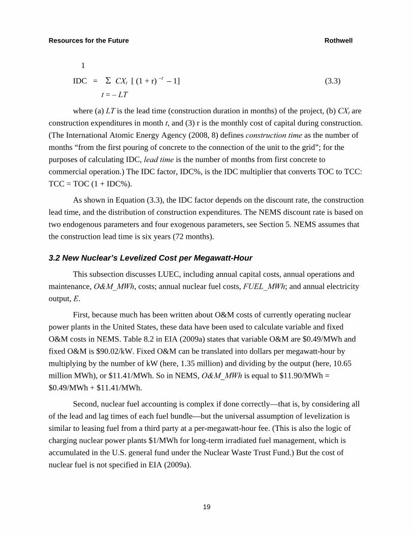
IDC = Σ CXt [ (1 + r) –t – 1] (3.3)
t = – LT
where (a) LT is the lead time (construction duration in months) of the project, (b) CXt are construction expenditures in month t, and (3) r is the monthly cost of capital during construction. (The International Atomic Energy Agency (2008, 8) defines construction time as the number of months “from the first pouring of concrete to the connection of the unit to the grid”; for the purposes of calculating IDC, lead time is the number of months from first concrete to commercial operation.) The IDC factor, IDC%, is the IDC multiplier that converts TOC to TCC: TCC = TOC (1 + IDC%).
As shown in Equation (3.3), the IDC factor depends on the discount rate, the construction lead time, and the distribution of construction expenditures. The NEMS discount rate is based on two endogenous parameters and four exogenous parameters, see Section 5. NEMS assumes that the construction lead time is six years (72 months).
3.2 New Nuclear’s Levelized Cost per Megawatt-Hour
This subsection discusses LUEC, including annual capital costs, annual operations and maintenance, O&M_MWh, costs; annual nuclear fuel costs, FUEL_MWh; and annual electricity output, E.
First, because much has been written about O&M costs of currently operating nuclear power plants in the United States, these data have been used to calculate variable and fixed O&M costs in NEMS. Table 8.2 in EIA (2009a) states that variable O&M are $0.49/MWh and fixed O&M is $90.02/kW. Fixed O&M can be translated into dollars per megawatt-hour by multiplying by the number of kW (here, 1.35 million) and dividing by the output (here, 10.65 million MWh), or $11.41/MWh. So in NEMS, O&M_MWh is equal to $11.90/MWh = $0.49/MWh + $11.41/MWh.
Second, nuclear fuel accounting is complex if done correctly—that is, by considering all of the lead and lag times of each fuel bundle—but the universal assumption of levelization is similar to leasing fuel from a third party at a per-megawatt-hour fee. (This is also the logic of charging nuclear power plants $1/MWh for long-term irradiated fuel management, which is accumulated in the U.S. general fund under the Nuclear Waste Trust Fund.) But the cost of nuclear fuel is not specified in EIA (2009a).
Resources for the Future Rothwell
20
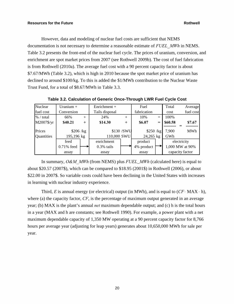
However, data and modeling of nuclear fuel costs are sufficient that NEMS documentation is not necessary to determine a reasonable estimate of FUEL_MWh in NEMS. Table 3.2 presents the front-end of the nuclear fuel cycle. The prices of uranium, conversion, and enrichment are spot market prices from 2007 (see Rothwell 2009b). The cost of fuel fabrication is from Rothwell (2010a). The average fuel cost with a 90 percent capacity factor is about $7.67/MWh (Table 3.2), which is high in 2010 because the spot market price of uranium has declined to around $100/kg. To this is added the $1/MWh contribution to the Nuclear Waste Trust Fund, for a total of $8.67/MWh in Table 3.3.
Table 3.2. Calculation of Generic Once-Through LWR Fuel Cycle Cost
Nuclear Uranium + Enrichment + Fuel Total Averagefuel cost Conversion Tails disposal fabrication cost fuel cost% / total 66% + 24% + 10% = 100%M2007$/yr $40.21 + $14.30 + $6.07 = $60.58 $7.67
--------- = ---------Prices $206 /kg $130 /SWU $250 /kg 7,900 MWhQuantities 195,196 kg 110,000 SWU 24,265 kg GWh
feed enrichment product electricity0.71% feed 0.3% tails 4% product 1,000 MW at 90%
assay assay assay capacity factor
In summary, O&M_MWh (from NEMS) plus FUEL_MWh (calculated here) is equal to about $20.57 (2007$), which can be compared to $18.95 (2001$) in Rothwell (2006), or about $22.00 in 2007$. So variable costs could have been declining in the United States with increases in learning with nuclear industry experience.
Third, E is annual energy (or electrical) output (in MWh), and is equal to (CF ⋅ MAX ⋅ h), where (a) the capacity factor, CF, is the percentage of maximum output generated in an average year; (b) MAX is the plant’s annual net maximum dependable output; and (c) h is the total hours in a year (MAX and h are constants; see Rothwell 1990). For example, a power plant with a net maximum dependable capacity of 1,350 MW operating at a 90 percent capacity factor for 8,766 hours per average year (adjusting for leap years) generates about 10,650,000 MWh for sale per year.

Resources for the Future Rothwell
21
Table 3.3. Real LUEC for New Nuclear Generation Following Assumptions in EIA (2009a)
R (% real) 8% 9% 10%
CRF(R,T) 8.17% 9.12% 10.09% TOC ($/kW) $3,318 $3,318 $3,318 IDC factor (%) 26.7% 30.4% 34.2% TCC ($/kW) $4,206 $4,328 $4,453 K@RISK ($M) $5,678 $5,843 $6,012 $K/year (M) $464 $533 $606 E (M MWh) 10.65 10.65 10.65 K/E ($/MWh) $43.57 $50.05 $56.93 +O&M/MWh $11.90 $11.90 $11.90 +FUEL/MWh $8.67 $8.67 $8.67 AC ($/MWh) $64.14 $70.62 $77.50 % increase 10.4% 10.1% 9.7%
Table 3.3 summarizes Sections 3.1 and 3.2. Assuming (a) real discount rates of 8, 9, and 10 percent; (b) a Capital-at-Risk of $6.012 billion (in 2007$); (c) an output of 10.65 million MWh; (d) an O&M_MWh of $11.90/MWh; and (e) a FUEL_MWh of $8.67/MWh, the AC would be between $64.14 and $77.50/MWh (2007$). Table 3.3 compares costs at various real discount rates. Here, on average, each 1 percent increase in the cost of capital increases LUEC by about 10 percent.
3.3 Is the NEMS Estimate of New Nuclear’s “Overnight” Cost Reasonable?
Several studies and cost estimates of new nuclear capacity have been published recently. To determine whether the NEMS $3,318/kW estimate is reasonable, this section reviews one of the most recent of these studies, Du and Parsons (2009), which updates MIT (2003). Du and Parsons base their estimate of nuclear power plant TOC on two data sets: (a) cost announcements for proposed nuclear plants in the United States, and (b) plants completed in Japan and Korea since 1994. Based on these data, they conclude that nuclear power plant costs doubled from 2002 to 2007 to $4,000/kW. Section 3.5 reviews Du and Parsons (2009).
Because there are multiple observations only on the cost estimate for twin AP1000s, the cost estimate here is based on AP1000a estimates only. The first cost observation for a twin AP1000a is Progress Energy’s Levy County Nuclear Power Plant in Florida with an escalated TOC of $9.4 billion from the World Nuclear Organization (WNO 2008, 10): “If built within 18 months of each other, the cost [would] total $9.4 [billion].”

Resources for the Future Rothwell
22
The second cost observation for a twin AP1000a is the SCE&G Virgil C. Summer Nuclear Generating Station with escalated TOC of $9.8 billion from Du and Parsons (2009, 14): “Other reports have given a $9.8 [billion] total that excludes the transmission upgrades and capital charges, but this sums together expenditures made in different years, including inflation projected over the various horizons.”
The third observation for a twin AP1000a is Georgia Power’s Vogtle Electric Generating Plant with an escalated TOC of $10.4 billion, also from Du and Parsons (2009, 15):
If we assume that these components are the same proportion of Georgia Power’s filings as they are for SCE&G, then the total project cost should be reduced to 74% of the reported figure, i.e., to an overnight cost of $10.439 [billion] or $4,745/kW in 2007 dollars. This leaves the Vogtle units with the highest forecasted overnight cost of the four newly planned sets.
(Note that an 80 percent loan guarantee of $8.33 billion implies escalated costs of $10.41 billion; so Du and Parsons’ estimate for Vogtle of $10.439 billion in 2007$ is nearly equal to this estimate in escalated dollars.)
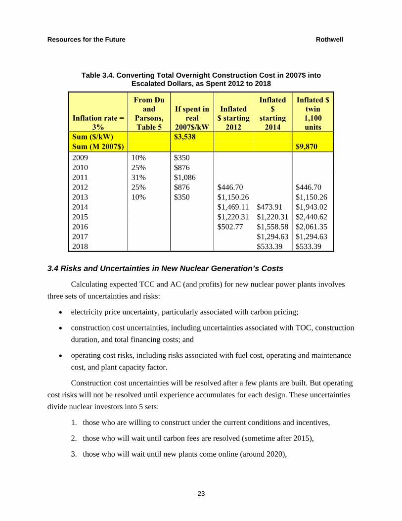
Assuming that the $10.4 billion TOC estimate (from August 2008) excludes IDC but includes escalation from 2008 through 2017, then it is comparable to the TOC estimates for Levy County ($9.4 billion in March 2008) and for Summer ($9.8 billion in May 2008). The average for these three observations on twin AP1000s built in the same region of the United States is $9,870 million in escalated dollars. This value for TOC in inflated dollars is deflated to 2007$ in Table 3.4. The deflated value is about $3,540/kW with a standard deviation of $190/kW and a range of $400/kW from $3,300/kW to $3,700/kW. The NEMS estimate of $3,318/kW is within this range, and thus could be reasonable based on the de-escalation of recent cost estimates for twin AP1000a plants. However, in EIA (2010), this value is increased to $3,820 in 2008$, or $3,700 in 2007$ (i.e., the Vogtle estimate). Although reasonable, it is the highest estimate available.
Resources for the Future Rothwell
23
Table 3.4. Converting Total Overnight Construction Cost in 2007$ into Escalated Dollars, as Spent 2012 to 2018
Inflation rate = 3%
From Du and
Parsons, Table 5
If spent in real
2007$/kW
Inflated $ starting
2012
Inflated $
starting 2014
Inflated $ twin 1,100 units
Sum ($/kW) $3,538 Sum (M 2007$) $9,870 2009 10% $350 2010 25% $876 2011 31% $1,086 2012 25% $876 $446.70 $446.70 2013 10% $350 $1,150.26 $1,150.26 2014 $1,469.11 $473.91 $1,943.02 2015 $1,220.31 $1,220.31 $2,440.62 2016 $502.77 $1,558.58 $2,061.35 2017 $1,294.63 $1,294.63 2018 $533.39 $533.39
3.4 Risks and Uncertainties in New Nuclear Generation’s Costs
Calculating expected TCC and AC (and profits) for new nuclear power plants involves three sets of uncertainties and risks:
• electricity price uncertainty, particularly associated with carbon pricing;
• construction cost uncertainties, including uncertainties associated with TOC, construction duration, and total financing costs; and
• operating cost risks, including risks associated with fuel cost, operating and maintenance cost, and plant capacity factor.
Construction cost uncertainties will be resolved after a few plants are built. But operating cost risks will not be resolved until experience accumulates for each design. These uncertainties divide nuclear investors into 5 sets:
1. those who are willing to construct under the current conditions and incentives,
2. those who will wait until carbon fees are resolved (sometime after 2015),
3. those who will wait until new plants come online (around 2020),
Resources for the Future Rothwell
24
4. those who will wait until there is sufficient experience with both construction and operation (around 2025), and
5. those who will wait until after 2030.
This limits the number of U.S. electric utilities that will construct nuclear plants before 2030. For example, consider the comments by Ralph Izzo, President and CEO of the New Jersey-based utility Public Service Enterprise Group (PSEG; which operates the Salem and Hope Creek nuclear power plants) signaling that he is in set 3, above, as quoted in Energy and Environment Daily (Ling 2009): “I think the biggest impediment of aggressive nuclear technology is its cost . . . PSEG is waiting for the first new reactors to be licensed and built before making any decision about new nuclear plants. The cost is not within my comfort level right now.”
Likewise, capital markets must evaluate these uncertainties to determine which uncertainties are manageable risks, and which involve unknown probabilities. Without an explicit model of the cost of debt and equity facing nuclear developers, capital markets are moving toward equilibrium costs of capital for new nuclear investment where risks are compensated by high required returns. These costs are likely to be higher for nuclear developers than for other electricity technology investors with similar levelized cost, if only because of nuclear generation’s large Capital-at-Risk.
Given that costs per kilowatt in NEMS appear to be reasonable in the 2009 version of NEMS, Section 4 discusses whether the NEMS estimated values for new nuclear capacity in 2020 (an additional 10 GW) and 2030 (no additional capacity) are reasonable.
3.5 A Review of Du and Parsons (2009)
Du and Parsons (2009) updated the total overnight cost for new nuclear power plants from its value in MIT (2003)—that is, $2,000 in 2002$. The paper begins by stating their conclusion that nuclear power plant overnight construction costs increased by 15 percent per year from 2002 to 2007, such that the best estimate of future total overnight cost is $4,000/kW in 2007$, as quoted by MIT (2009) and others. Du and Parsons (2009, 8–9, emphasis added) apply
a 15% per annum nuclear power capital cost inflation factor to put these [Japanese and Korean figures from MIT (2003)] into 2007 dollars. We discuss the choice of this escalation factor below. Therefore, these costs would range from $3,222/kW to $5,072/kW expressed in 2007 dollars. The average is $4,000/kW, expressed in 2007 dollars.

Resources for the Future Rothwell
25
However, average overnight construction costs changed little in Japan and Korea before 2003 (when the average was about $2,000/kW) to after 2003 (when the average was about $2,175/kW). See Figure 3.1, where the Japanese and Korean cost data have been discounted to 2002$, as in MIT (2003), instead of by 15 percent to 2007$. There is no significant difference between the mean before 2003, which is quoted in MIT (2003), and the mean after 2003, which Du and Parsons add to the MIT (2003) analysis. The real escalation rate is in the neighborhood of 0 percent.
Figure 3.1. Cost per Kilowatt for Japanese and Korean Plants in 2002$
$1,500
$1,700
$1,900
$2,100
$2,300
$2,500
$2,700
$2,900
1992 1994 1996 1998 2000 2002 2004 2006 2008
2002
$/kW
Overall mean = $2,075
Sample MIT (2003)Sample mean = $2,000
Sample MIT (2009)Sample mean = $2,175
ABWR
ABWR
ABWR
ABWR
Note: All ABWRs were built in Japan. Source: Du and Parsons (2009).
The costs after 2003 appear to be lower than those before 2003:
Since the publication of the MIT (2003) study, over the years 2004–2006, five additional units have been completed in Japan and Korea. . . . These costs are denominated in the various years in which each plant was completed, and so we apply the 15% inflation rate . . . The overnight costs on these units range between $2,357/kW and $3,357/kW, expressed in 2007 dollars. The average is just under $3,000/kW, expressed in 2007 dollars. This more recent range is lower than the range for the earlier Japanese and Korean builds, perhaps reflecting continuing improvements in construction or other design factors. (Du and Parsons 2009, 9, emphasis added)
Resources for the Future Rothwell
26
If there were continuing improvements in construction, it is unlikely that the escalation rate would increase at 15 percent from 2002 to 2007. Because the real escalation rate is 0 percent, escalating the older data by 15 percent over five years doubles it, whereas escalating the newer data over fewer years increases it by only 50 percent. This leads to the contradiction between $4,000/kW for older Asian units and $3,000/kW for newer Asian units.
After escalating Asian nuclear power plant cost data using the assumed 15 percent escalation rate, Du and Parsons then assemble a data set of six observations to prove that $4,000/kW (and the 15 percent escalation rate) is the best current estimate of overnight nuclear costs in the United States. They begin by updating the overnight costs (see Table 3.1) in TVA (2005), a DOE-funded study of constructing an ABWR at TVA’s Bellefonte site, based on earlier studies under the NP2010 Program. Du and Parsons (2009, 12, emphasis added) state that,
The published figure of $1,611/kW, however, is for [engineering, procurement, and construction, EPC] overnight costs only, and does not include owner’s costs. Therefore, we add 20% to the reported figure in order to produce a full overnight cost of $1,933/kW as reported in 2004 dollars. Escalated to 2007 dollars using our 15% rate, the overnight cost is $2,930.
Here, Du and Parsons use their conclusion of the 15 percent escalation rate to update the cost data to 2007. This would bias their mean cost estimate had they used this value in their calculations. But this observation is not used in determining their central value because “it was not an actual build proposal and was for an earlier year” (Du and Parsons 2009, 16).
Du and Parsons’ second observation is on Florida Power & Light’s (FPL’s) cost estimate for either two AP1000s or two ESBWRs at its Turkey Point site. The cost estimate was not for either technology, but was done by adjusting the TVA (2005) ABWR cost estimate. However, Du and Parsons (2009, 13) determine “the filings give us sufficient information to back out these components and arrive at a full overnight cost of $3,530/kW in 2007 dollars.” (Their central value can be calculated with or without this observation.)
Du and Parsons (2009, 13) examine three cost estimates for twin AP1000s. Their first observation for twin AP1000s is Levy County, Florida:
Progress Energy filed the petition in March 2008 looking to generation starting in 2016 for the first unit and 2017 for the second. Excluding capital and other charges, the total project cost is $9.304 [billion] for both units expressed in 2007 dollars. This translates to $4,206/kW in 2007 dollars.
But the conclusion that TOC are $9.304 billion in 2007$ is inconsistent with WNO (2008, 10), where the total of $9.4 billion is in escalated dollars:

Resources for the Future Rothwell
27
If built within 18 months of each other, the cost for the first would be $5,144/kW and the second $3,376/kW (average $4,260/kW) – total $9.4 [billion]. . . . At the end of December 2008 the company signed an EPC contract for $7.65B ($3,462/kW) of an overall project cost of about $14 [billion].
The second observation on twin AP1000s is SCE&G’s Summer in South Carolina (where Unit 2 is scheduled for completion in 2016, and Unit 3 is scheduled for completion in 2019):
Other reports have given a $9.8 [billion] total that excludes the transmission upgrades and capital charges, but this sums together expenditures made in different years including inflation projected over the various horizons. We use the detailed filing to exclude capital and other charges and to denominate the costs in 2007 dollars. We calculate a total project cost of $8.459 [billion] for both units expressed in 2007 dollars. This translates to $3,787/kW in 2007 dollars.
Assuming that the $9.8 billion TOC estimate excludes IDC but includes escalation from 2008 through 2019 and that the $8.459 billion TOC estimate excludes both IDC and escalation from 2008 through 2019, then the deflation factor (bringing expenditures during a decade into 2007$) is 87.3 percent. This factor would be appropriate for bringing construction expenditures starting in 2009 back to 2007, but not for expenditures starting in 2012 (see Table 3.5, where $4,000/$4,505 = 89 percent). Du and Parsons’ deflating factor should be closer to 78 percent (= $4,000/$5,123).
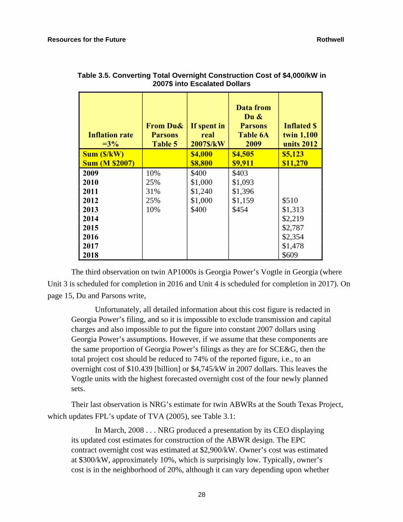
To understand how Du and Parsons estimated deflated values, Table 3.5 reproduces Du and Parsons’ spreadsheet for determining LUEC, “Table 6A: Cost Cash Flows and Depreciation at a Nuclear Power Plant ($ millions).” The value of $4,000/kW in 2007$ inflates to $4,505/kW if spending begins in 2009 (see Table 3.5., fourth column). However, because no standardized construction (and operating) license will be issued before 2012, the last column of Table 3.5 is more appropriate.
Resources for the Future Rothwell
28
Table 3.5. Converting Total Overnight Construction Cost of $4,000/kW in 2007$ into Escalated Dollars
Inflation rate =3%
From Du& Parsons Table 5
If spent in real
2007$/kW
Data from Du &
Parsons Table 6A
2009
Inflated $ twin 1,100 units 2012
Sum ($/kW) $4,000 $4,505 $5,123 Sum (M $2007) $8,800 $9,911 $11,270 2009 10% $400 $403 2010 25% $1,000 $1,093 2011 31% $1,240 $1,396 2012 25% $1,000 $1,159 $510 2013 10% $400 $454 $1,313 2014 $2,219 2015 $2,787 2016 $2,354 2017 $1,478 2018 $609
The third observation on twin AP1000s is Georgia Power’s Vogtle in Georgia (where Unit 3 is scheduled for completion in 2016 and Unit 4 is scheduled for completion in 2017). On page 15, Du and Parsons write,
Unfortunately, all detailed information about this cost figure is redacted in Georgia Power’s filing, and so it is impossible to exclude transmission and capital charges and also impossible to put the figure into constant 2007 dollars using Georgia Power’s assumptions. However, if we assume that these components are the same proportion of Georgia Power’s filings as they are for SCE&G, then the total project cost should be reduced to 74% of the reported figure, i.e., to an overnight cost of $10.439 [billion] or $4,745/kW in 2007 dollars. This leaves the Vogtle units with the highest forecasted overnight cost of the four newly planned sets.
Their last observation is NRG’s estimate for twin ABWRs at the South Texas Project, which updates FPL’s update of TVA (2005), see Table 3.1:
In March, 2008 . . . NRG produced a presentation by its CEO displaying its updated cost estimates for construction of the ABWR design. The EPC contract overnight cost was estimated at $2,900/kW. Owner’s cost was estimated at $300/kW, approximately 10%, which is surprisingly low. Typically, owner’s cost is in the neighborhood of 20%, although it can vary depending upon whether
Resources for the Future Rothwell
29
a unit is being built in a greenfield site and other factors. Transmission costs are separate and not included in NRG’s figure, as are IDC. Adding another 10% for owner’s costs brings the total cost to $3,480/kW. (Du and Parsons 2009, 16)
But on page 6, Du and Parsons state “[a] 20% figure is a reasonable assumption absent specific information for a given plant.” Although this 20 percent value is not referenced (see Delene and Hudson 1990, suggesting 15 percent), it is used, even though specific information for this plant contradicts their statement on page 6.
With these data, Du and Parsons (2009, 16) find that expected new nuclear capacity overnight cost lies between about $3,500/kW and $4,800/kW (see Table 4 in Du and Parsons 2009). If the Turkey Point estimate is included, the mean is $3,950/kW. If it is excluded, the mean is $4,055/kW. Taking a central value between these two means, Du and Parsons (2009, 16–17) conclude,
The overnight cost of the proposed units—i.e., excluding the TVA estimate as it was not an actual build proposal and was for an earlier year—lie between $3,500 and $4,800/kW, denominated in 2007 dollars. . . . Based on this data, and in light of the experience of actual builds in Japan and Korea, for the rest of this paper we choose to use $4,000/kW in 2007 dollars as a central value for our comparisons. . . . Using the MIT (2003) estimate of $2,000/kW in 2002 dollars, and a central estimate of $4,000/kW in 2007 dollars, our results suggest an annual rate of increase in overnight costs of approximately 15% during this period. This represents a sizeable premium to the general rate of inflation—the 3% per annum mentioned above for the GDP deflator. (emphasis added)
Because nominal values were incorrectly converted to real values, the Du and Parsons central value is at least 12.5 percent too high. Because the real rate of escalation in Asia was near 0 percent, the “experience of actual builds in Japan and Korea” does not support the conclusion of a 15 percent escalation rate.
4. Expected New Nuclear Capacities in 2020 and 2030
This section discusses whether NEMS-RFF projections of nuclear capacity are reasonable in the following scenarios: Core_1: Obama CAFE Target; Core_2: Original Core 2 with Two Billion Ton Limit on Offsets; and Core_2n: Revised Core 2 with One Billion Ton Limit on Offsets.
Core_1 estimates about 10 GW of new nuclear capacity by 2020, and no net additions between 2020 and 2030. With a CO2 control program, Core_2 scenarios estimate about 48 GW
Resources for the Future Rothwell
30
of new nuclear capacity by 2030. This section discusses whether Core_1 yields reasonable estimates under current federal incentives for nuclear capacity.
4.1 New Nuclear Capacity in NEMS-RFF under Base Case (Core_1)
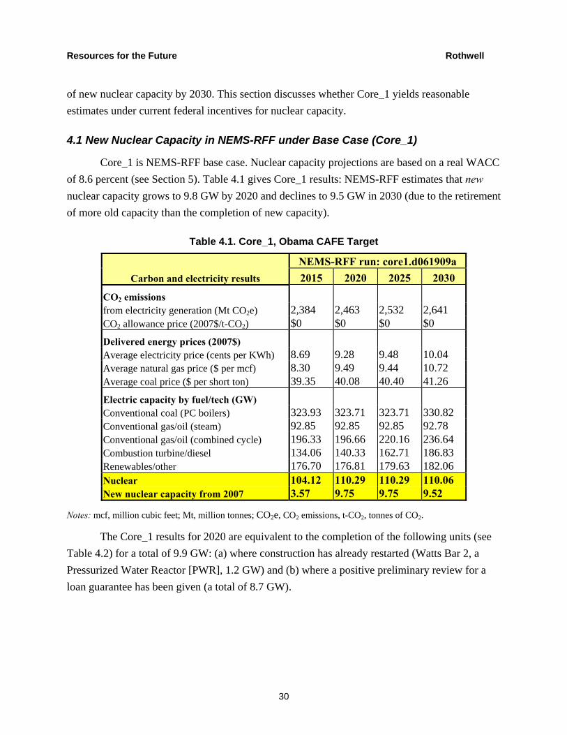
Core_1 is NEMS-RFF base case. Nuclear capacity projections are based on a real WACC of 8.6 percent (see Section 5). Table 4.1 gives Core_1 results: NEMS-RFF estimates that new nuclear capacity grows to 9.8 GW by 2020 and declines to 9.5 GW in 2030 (due to the retirement of more old capacity than the completion of new capacity).
Table 4.1. Core_1, Obama CAFE Target
Carbon and electricity results NEMS-RFF run: core1.d061909a 2015 2020 2025 2030
CO2 emissions from electricity generation (Mt CO2e) 2,384 2,463 2,532 2,641 CO2 allowance price (2007$/t-CO2) $0 $0 $0 $0 Delivered energy prices (2007$) Average electricity price (cents per KWh) 8.69 9.28 9.48 10.04 Average natural gas price ($ per mcf) 8.30 9.49 9.44 10.72 Average coal price ($ per short ton) 39.35 40.08 40.40 41.26 Electric capacity by fuel/tech (GW) Conventional coal (PC boilers) 323.93 323.71 323.71 330.82 Conventional gas/oil (steam) 92.85 92.85 92.85 92.78 Conventional gas/oil (combined cycle) 196.33 196.66 220.16 236.64 Combustion turbine/diesel 134.06 140.33 162.71 186.83 Renewables/other 176.70 176.81 179.63 182.06 Nuclear 104.12 110.29 110.29 110.06 New nuclear capacity from 2007 3.57 9.75 9.75 9.52
Notes: mcf, million cubic feet; Mt, million tonnes; CO2e, CO2 emissions, t-CO2, tonnes of CO2.
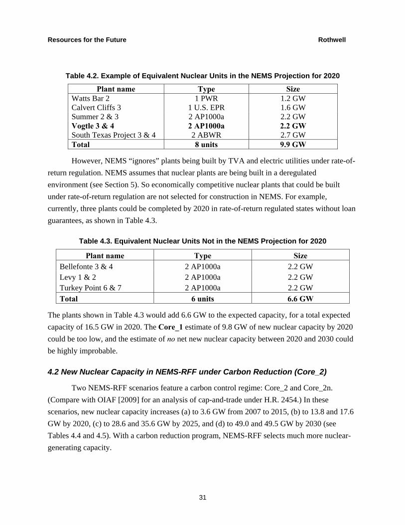
The Core_1 results for 2020 are equivalent to the completion of the following units (see Table 4.2) for a total of 9.9 GW: (a) where construction has already restarted (Watts Bar 2, a Pressurized Water Reactor [PWR], 1.2 GW) and (b) where a positive preliminary review for a loan guarantee has been given (a total of 8.7 GW).
Resources for the Future Rothwell
31
Table 4.2. Example of Equivalent Nuclear Units in the NEMS Projection for 2020
Plant name Type Size Watts Bar 2 1 PWR 1.2 GW Calvert Cliffs 3 1 U.S. EPR 1.6 GW Summer 2 & 3 2 AP1000a 2.2 GW Vogtle 3 & 4 2 AP1000a 2.2 GW South Texas Project 3 & 4 2 ABWR 2.7 GW Total 8 units 9.9 GW
However, NEMS “ignores” plants being built by TVA and electric utilities under rate-of-return regulation. NEMS assumes that nuclear plants are being built in a deregulated environment (see Section 5). So economically competitive nuclear plants that could be built under rate-of-return regulation are not selected for construction in NEMS. For example, currently, three plants could be completed by 2020 in rate-of-return regulated states without loan guarantees, as shown in Table 4.3.
Table 4.3. Equivalent Nuclear Units Not in the NEMS Projection for 2020
Plant name Type Size Bellefonte 3 & 4 2 AP1000a 2.2 GW Levy 1 & 2 2 AP1000a 2.2 GW Turkey Point 6 & 7 2 AP1000a 2.2 GW Total 6 units 6.6 GW
The plants shown in Table 4.3 would add 6.6 GW to the expected capacity, for a total expected capacity of 16.5 GW in 2020. The Core_1 estimate of 9.8 GW of new nuclear capacity by 2020 could be too low, and the estimate of no net new nuclear capacity between 2020 and 2030 could be highly improbable.
4.2 New Nuclear Capacity in NEMS-RFF under Carbon Reduction (Core_2)
Two NEMS-RFF scenarios feature a carbon control regime: Core_2 and Core_2n. (Compare with OIAF [2009] for an analysis of cap-and-trade under H.R. 2454.) In these scenarios, new nuclear capacity increases (a) to 3.6 GW from 2007 to 2015, (b) to 13.8 and 17.6 GW by 2020, (c) to 28.6 and 35.6 GW by 2025, and (d) to 49.0 and 49.5 GW by 2030 (see Tables 4.4 and 4.5). With a carbon reduction program, NEMS-RFF selects much more nuclear-generating capacity.
Resources for the Future Rothwell
32
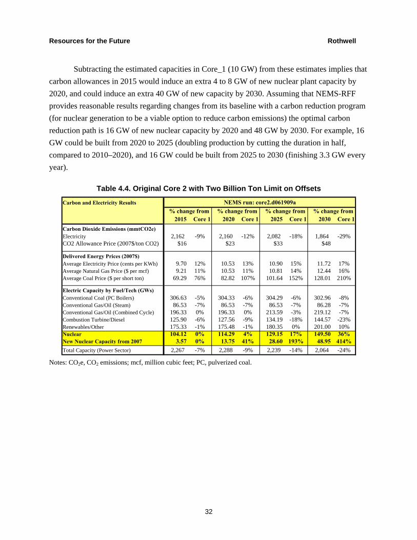
Subtracting the estimated capacities in Core_1 (10 GW) from these estimates implies that carbon allowances in 2015 would induce an extra 4 to 8 GW of new nuclear plant capacity by 2020, and could induce an extra 40 GW of new capacity by 2030. Assuming that NEMS-RFF provides reasonable results regarding changes from its baseline with a carbon reduction program (for nuclear generation to be a viable option to reduce carbon emissions) the optimal carbon reduction path is 16 GW of new nuclear capacity by 2020 and 48 GW by 2030. For example, 16 GW could be built from 2020 to 2025 (doubling production by cutting the duration in half, compared to 2010–2020), and 16 GW could be built from 2025 to 2030 (finishing 3.3 GW every year).
Table 4.4. Original Core 2 with Two Billion Ton Limit on Offsets
Carbon and Electricity Results NEMS run: core2.d061909a % change from % change from % change from % change from
2015 Core 1 2020 Core 1 2025 Core 1 2030 Core 1Carbon Dioxide Emissions (mmtCO2e)Electricity 2,162 -9% 2,160 -12% 2,082 -18% 1,864 -29%CO2 Allowance Price (2007$/ton CO2) $16 $23 $33 $48
Delivered Energy Prices (2007$)Average Electricity Price (cents per KWh) 9.70 12% 10.53 13% 10.90 15% 11.72 17%Average Natural Gas Price ($ per mcf) 9.21 11% 10.53 11% 10.81 14% 12.44 16%Average Coal Price ($ per short ton) 69.29 76% 82.82 107% 101.64 152% 128.01 210%
Electric Capacity by Fuel/Tech (GWs)Conventional Coal (PC Boilers) 306.63 -5% 304.33 -6% 304.29 -6% 302.96 -8%Conventional Gas/Oil (Steam) 86.53 -7% 86.53 -7% 86.53 -7% 86.28 -7%Conventional Gas/Oil (Combined Cycle) 196.33 0% 196.33 0% 213.59 -3% 219.12 -7%Combustion Turbine/Diesel 125.90 -6% 127.56 -9% 134.19 -18% 144.57 -23%Renewables/Other 175.33 -1% 175.48 -1% 180.35 0% 201.00 10%Nuclear 104.12 0% 114.29 4% 129.15 17% 149.50 36%New Nuclear Capacity from 2007 3.57 0% 13.75 41% 28.60 193% 48.95 414%Total Capacity (Power Sector) 2,267 -7% 2,288 -9% 2,239 -14% 2,064 -24%
Notes: CO2e, CO2 emissions; mcf, million cubic feet; PC, pulverized coal.

Resources for the Future Rothwell
33
Table 4.5. Revised Core 2 with One Billion Ton Limit on Offsets
Carbon and Electricity Results NEMS Run: core2n.d070609a % change from % change from % change from % change from
2015 Core 1 2020 Core 1 2025 Core 1 2030 Core 1Carbon Dioxide Emissions (mmtCO2e)Electricity 2,053 -14% 2,022 -18% 1,832 -28% 1,447 -45%CO2 Allowance Price (2007$/ton CO2) $23 $33 $47 $67
Delivered Energy Prices (2007$)Average Electricity Price (cents per KWh) 10.13 17% 11.02 19% 11.45 21% 12.75 27%Average Natural Gas Price ($ per mcf) 9.63 16% 10.99 16% 11.53 22% 13.65 27%Average Coal Price ($ per short ton) 81.60 107% 100.58 151% 126.02 212% 164.83 300%
Electric Capacity by Fuel/Tech (GWs)Conventional Coal (PC Boilers) 294.96 -9% 289.87 -10% 289.14 -11% 257.79 -22%Conventional Gas/Oil (Steam) 85.40 -8% 85.40 -8% 85.40 -8% 85.21 -8%Conventional Gas/Oil (Combined Cycle) 196.33 0% 196.33 0% 211.75 -4% 228.11 -4%Combustion Turbine/Diesel 128.06 -4% 127.59 -9% 130.33 -20% 137.67 -26%Renewables/Other 176.35 0% 176.72 0% 187.31 4% 230.99 27%Nuclear 104.12 0% 118.16 7% 136.11 23% 150.07 36%New Nuclear Capacity from 2007 3.57 0% 17.61 81% 35.56 265% 49.53 420%Total Capacity (Power Sector) 2,177 -11% 2,178 -14% 2,028 -22% 1,705 -37%
Notes: CO2e, CO2 emissions; mcf, million cubic feet; PC, pulverized coal.
4.3 Is the Estimate of Nuclear Capacity under Core_1 Reasonable?
Are Core_1 results regarding new nuclear capacity—that is, 10 GW by 2020 and 2 gross GW through 2030—reasonable? This subsection compares NEMS-RFF results with a nuclear industry expert elicitation of expected probabilities of nuclear power plant completions by 2020 and by 2030. If all units now proposed were completed by 2020, new nuclear capacity could be as high as 36.3 GW.
Twenty experts were polled. They were sent Table 2.4 (without bold or italics or the sum in the last column) and were asked to give their expected probability of completion for each plant in 2020 and in 2030. (All 100 percent probabilities of completion were converted to 99 percent and all 0 percent probabilities were converted to 1 percent to allow for the calculation of log odds ratios; see Section 4.5. Expert 0, the null hypothesis, gives the NEMS expectations.)
Table 4.6 presents their expected probability of completion in 2020 multiplied by the size of the plant in GW (“expected nuclear capacity additions”). (Although fractions of plants might seem nonsensical, because there is no standard plant size, NEMS constructs fractions of nuclear power plants; see Table 5.4.) The expected new nuclear capacity in 2020 is 13.9 GW with a median of 12.0 GW. The Core_1 result of 10 GW by 2020 is similar to these expectations. Thus, the NEMS-RFF estimate for 2020 is reasonable. Section 6 will interpret the new nuclear power

Resources for the Future Rothwell
34
units coming into commercial production from 2017 to 2020 in Core_1 (i.e., 6.2 GW) as the reasonable result of EPAct05+ incentives.
Table 4.6 also presents these experts’ expected nuclear capacity additions between 2020 and 2030 (in column 3) and by 2030 (in column 4). The average expected addition to capacity between 2020 and 2030 is 9.3 GW with a median of 9.7 GW. The average expected new nuclear capacity in 2030 is 23.1 GW with a median of 23.1 GW. (These experts were not allowed to speculate on the probabilities of completion of plants not yet proposed; so these could be conservative expectations for this group.)
The Core_1 estimate of no net additional new nuclear capacity between 2020 and 2030 is unreasonable, given the findings from this sample of nuclear generation industry experts. To avoid basing policy analysis on baseline estimates, Sections 5 and 6 subtract Core_1 baseline estimates from the results of other scenarios to examine how changes in the cost of capital influence new nuclear capacity. Section 5 examines whether the cost of capital for nuclear power plant investors is reasonable in NEMS.
However, because these experts are so diverse in their estimated probabilities of the completion of particular units, Section 4.5 investigates whether these subjective probabilities are consistent with rational underlying evaluation functions. The section finds that the experts are consistent and rely primarily on whether the nuclear plant project had a positive preliminary review for a loan guarantee.
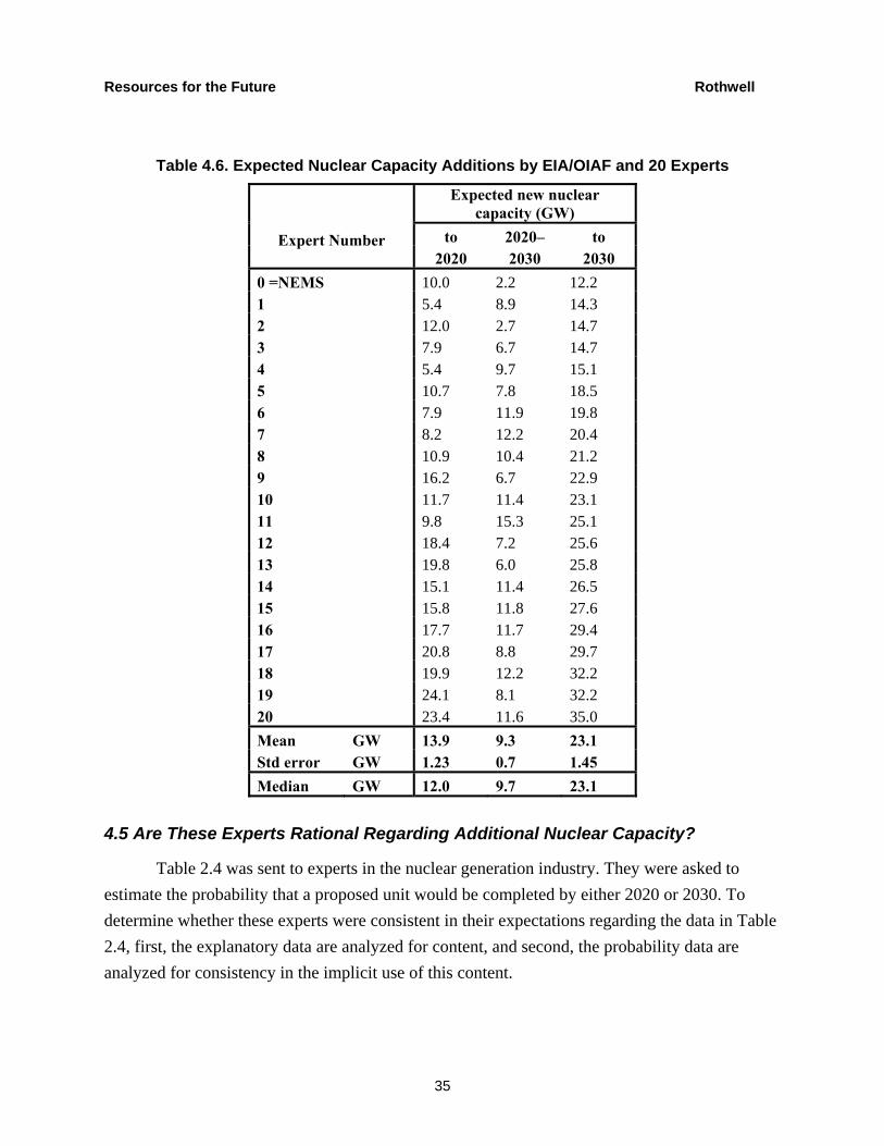
Resources for the Future Rothwell
35
Table 4.6. Expected Nuclear Capacity Additions by EIA/OIAF and 20 Experts
Expert Number
Expected new nuclear capacity (GW)
to 2020– to 2020 2030 2030
0 =NEMS 10.0 2.2 12.2 1 5.4 8.9 14.3 2 12.0 2.7 14.7 3 7.9 6.7 14.7 4 5.4 9.7 15.1 5 10.7 7.8 18.5 6 7.9 11.9 19.8 7 8.2 12.2 20.4 8 10.9 10.4 21.2 9 16.2 6.7 22.9 10 11.7 11.4 23.1 11 9.8 15.3 25.1 12 18.4 7.2 25.6 13 19.8 6.0 25.8 14 15.1 11.4 26.5 15 15.8 11.8 27.6 16 17.7 11.7 29.4 17 20.8 8.8 29.7 18 19.9 12.2 32.2 19 24.1 8.1 32.2 20 23.4 11.6 35.0 Mean GW 13.9 9.3 23.1 Std error GW 1.23 0.7 1.45 Median GW 12.0 9.7 23.1
4.5 Are These Experts Rational Regarding Additional Nuclear Capacity?
Table 2.4 was sent to experts in the nuclear generation industry. They were asked to estimate the probability that a proposed unit would be completed by either 2020 or 2030. To determine whether these experts were consistent in their expectations regarding the data in Table 2.4, first, the explanatory data are analyzed for content, and second, the probability data are analyzed for consistency in the implicit use of this content.

Resources for the Future Rothwell
36
Regarding the explanatory variables, much of the information in Table 2.4 is redundant. For example, all but one plant (Summer) that is being considered for a loan guarantee is also a Reference COL. A factor analysis conducted with these variables is presented in Tables 4.7 and 4.8.
Table 4.7. Correlations among Explanatory Variables in Table 2.4
EPC LOAN R-COL OLD REG BOND EPC 1.000 0.775 0.445 0.194 0.142 0.086 LOAN 0.775 1.000 0.486 0.397 –0.042 0.048 R-COL 0.445 0.486 1.000 0.474 –0.386 0.132 OLD 0.194 0.397 0.474 1.000 –0.084 0.044 REG 0.142 –0.042 –0.386 –0.084 1.000 0.464 BOND 0.086 0.048 0.132 0.044 0.464 1.000
Notes: Light gray typeface indicates little correlation. Variable descriptions: EPC indicates whether an engineering, procurement, and construction contract has been signed; LOAN indicates whether DOE has indicated that it might offer a loan guarantee to a unit’s builder; R-COL indicates whether a unit is a part of a reference construction and operating license; OLD indicates whether a unit is being built at an existing site; REG indicates whether a unit is being built in a state with ROE regulation; and BOND indicates whether the bond rating of a unit’s owner is in the “A” range, such as Aaa.
Table 4.8. Underlying Factors among Explanatory Variables in Table 2.4
Variable Factor 1 Factor 2
EPC 0.789 0.275
LOAN 0.872 0.103
R-COL 0.795 –0.232
OLD 0.621 –0.107
REG –0.159 0.900
BOND 0.117 0.761
Notes: Light gray typeface indicates little correlation. Variable descriptions: EPC indicates whether an engineering, procurement, and construction contract has been signed; LOAN indicates whether DOE has indicated that it might offer a loan guarantee to a unit’s builder; R-COL indicates whether a unit is a part of a reference construction and operating license; OLD indicates whether a unit is being built at an existing site; REG indicates whether a unit is being built in a state with ROE regulation; and BOND indicates whether the bond rating of a unit’s owner is in the “A” range, such as Aaa.
These tables distinguish between two groups of variables: (a) one group that measures “progress to completion” and includes whether the unit is a Reference COL (R-COL) at an existing site (OLD) with an EPC contract with a high likelihood of receiving a DOE loan

Resources for the Future Rothwell
37
guarantee (LOAN); and (b) another group that measures the “financial riskiness” of a project based on whether a plant will be built under rate-of-return regulation (REG) and whether the owner has a high bond rating (BOND). These results imply that most of the information can be represented by two explanatory variables.
In this set of variables, the most policy-relevant variable is whether the plant will receive loan guarantees from DOE. Also, federal policy can influence the perceived financial riskiness of nuclear projects, thereby influencing the bond rating, for example, by implementing an effective carbon control regime, increasing the NPV of all carbon-free electricity-generating resources. Do these experts consistently incorporate LOAN and BOND information in their evaluations?
An Appendix (available from the author on request) presents the experts’ expected probabilities of completion for each unit in 2020 and in 2030. To test whether these experts consistently use the available information, the subjective probabilities, Pi, are converted to their “log odds ratios”—that is, ln [Pi / (1 – Pi)]—to allow the application of ordinary least squares (OLS). (The estimator is a linearized logit model.) These converted values can be regressed on LOAN and BOND to determine how these variables influence the experts’ expected probabilities of completion. OLS parameters are available in the Appendix.
The OLS parameters can be converted into probabilities as functions of whether the nuclear project has a good bond rating (BOND = 1) and might get a federal loan guarantee (LOAN = 1). Tables 4.9 and 4.10 present these predicted probabilities of completion (based on the OLS results) by 2020 and by 2030. The tables are divided into two sections, where the baseline probability is less than or greater than 50 percent. Except for Experts 3 and 18, all predicted probabilities are higher for units with preliminary favorable reviews for a loan guarantee than for units with high bond ratings. The predicted probability of completion in 2020 for a unit with a high bond rating and a loan guarantee varies between 46.8 percent for Expert 11 and 99.6 percent for Expert 1. The only “inconsistency” is Expert 3’s disregard for the loan guarantee indicator.
Because of the lack of major inconsistencies in these data or results, I conclude that the experts’ collective expectation defines a reasoned consensus of a new nuclear capacity of about 12–16 GW in 2020. This is approximately equal to (a) 1.2 GW with the completion of Watts Bar 2, plus (b) 8.7 GW with the completion of those plants, or similar ones, that have received initial positive loan guarantee reviews, plus (c) 6.6 GW for those plants being built under regulation. Although the estimate of 10 GW by 2020 is pessimistic, it is reasonable. But the estimate that there will be no new net nuclear capacity built from 2020 to 2030 is not reasonable.
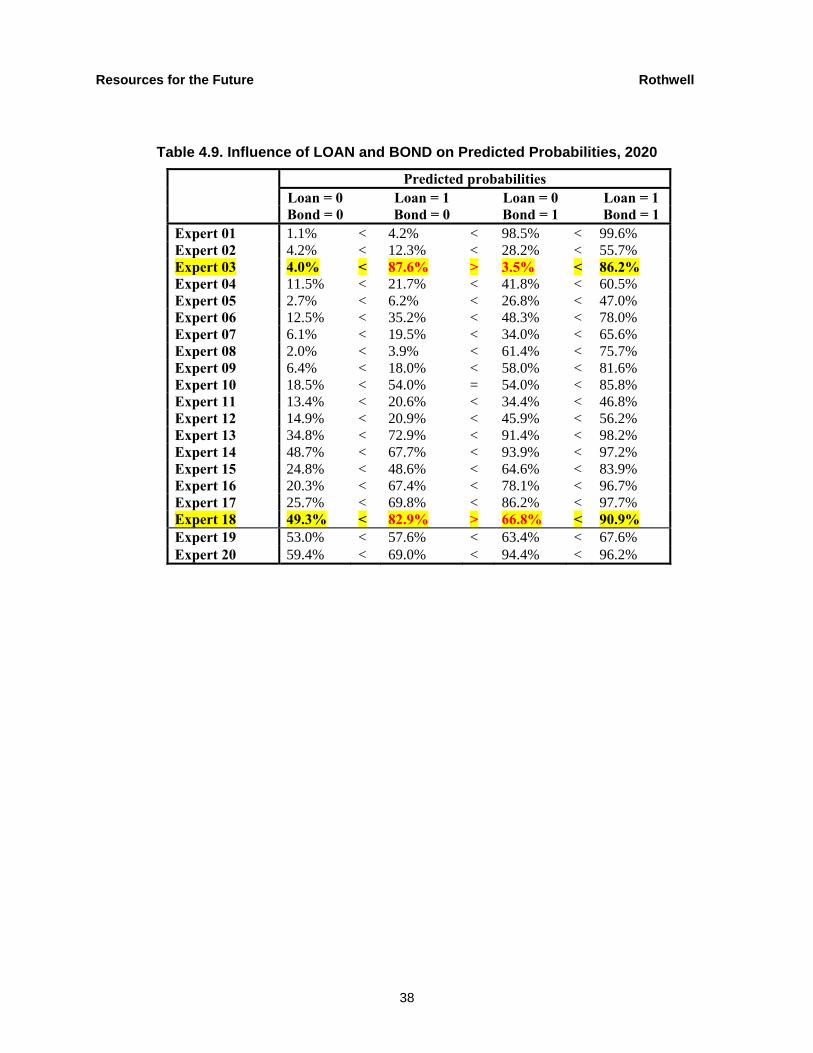
Resources for the Future Rothwell
38
Table 4.9. Influence of LOAN and BOND on Predicted Probabilities, 2020
Predicted probabilities
Loan = 0 Loan = 1 Loan = 0 Loan = 1 Bond = 0 Bond = 0 Bond = 1 Bond = 1
Expert 01 1.1% < 4.2% < 98.5% < 99.6% Expert 02 4.2% < 12.3% < 28.2% < 55.7% Expert 03 4.0% < 87.6% > 3.5% < 86.2% Expert 04 11.5% < 21.7% < 41.8% < 60.5% Expert 05 2.7% < 6.2% < 26.8% < 47.0% Expert 06 12.5% < 35.2% < 48.3% < 78.0% Expert 07 6.1% < 19.5% < 34.0% < 65.6% Expert 08 2.0% < 3.9% < 61.4% < 75.7% Expert 09 6.4% < 18.0% < 58.0% < 81.6% Expert 10 18.5% < 54.0% = 54.0% < 85.8% Expert 11 13.4% < 20.6% < 34.4% < 46.8% Expert 12 14.9% < 20.9% < 45.9% < 56.2% Expert 13 34.8% < 72.9% < 91.4% < 98.2% Expert 14 48.7% < 67.7% < 93.9% < 97.2% Expert 15 24.8% < 48.6% < 64.6% < 83.9% Expert 16 20.3% < 67.4% < 78.1% < 96.7% Expert 17 25.7% < 69.8% < 86.2% < 97.7% Expert 18 49.3% < 82.9% > 66.8% < 90.9% Expert 19 53.0% < 57.6% < 63.4% < 67.6% Expert 20 59.4% < 69.0% < 94.4% < 96.2%

Resources for the Future Rothwell
39
Table 4.10. Influence of LOAN and BOND on Predicted Probabilities, 2030
Predicted probabilities Loan = 0 Loan = 1 Loan = 0 Loan = 1Bond = 0 Bond = 0 Bond = 1 Bond = 1
Expert 01 3% < 5% < 99% < 99% Expert 02 27% < 39% < 65% < 76% Expert 03 9% < 99% > 5% < 98.5% Expert 04 20% < 54% < 83% < 96% Expert 05 21% < 76% > 66% < 96% Expert 06 39% < 66% < 69% < 87% Expert 07 50% < 60% < 64% < 72% Expert 08 27% < 62% < 98% < 100% Expert 09 41% < 89% < 98% < 100% Expert 10 34% < 85% < 85% < 98% Expert 11 53% < 90% < 98% < 100% Expert 12 66% < 77% < 84% < 90% Expert 13 70% < 86% < 96% < 99% Expert 14 75% < 85% < 97% < 98.3% Expert 15 69% < 87% < 91% < 97% Expert 16 72% < 96% = 96% < 100% Expert 17 81% < 94% < 96% < 99% Expert 18 83% < 93% > 83% < 93% Expert 19 88% < 89% < 93% < 93% Expert 20 90% < 92% < 99% < 99%
5. The Cost of Capital for New Nuclear Plant Owners in NEMS
5.1 Nuclear Generation’s Weighted Average Cost of Capital in NEMS
The cost of capital for nuclear power plant investment in NEMS is “assumed to be about 17% ROE (Return-on-Equity) and 8%+ for Debt Costs” (email sent by OnLocation to G.S. Rothwell, July 26, 2009). To determine the WACC, EIA (2009b, Appendix 3.D, “Cost of Capital,” 84) describes how WACC is determined for each year in NEMS for all electric utility investments by the Electricity Capacity Planning (ECP) submodule:
The model performs a discounted cash flow analysis of the costs of building and operating power plants over the next 20 years and chooses the least cost mix of options. The ECP assumes that building power plants will take place in a competitive environment rather than in a rate base or regulated environment. . . . The discount rate (WACC) is a very important component because the rate reflects the riskiness of the investment and affects [the] mix of capacity additions. . . . small changes in the weighted average cost [of] capital lead to huge changes in capital intensive capacity additions. (emphasis added)
Resources for the Future Rothwell
40
Also, the NEMS WACC is determined under the following assumptions (EIA 2009b, 85):
(1) Power generating industry is competitive. Thus, investments for power plants are made in [a] competitive environment that includes certain risks.
(2) Different generating technologies have the same risk treatment in investment for capital budgeting purposes. That is, the required rate of return (WACC) on investment is the same for all projects.
(3) The discount rate (WACC) is different for each year.
These statements point to the primary contradiction in the ECP submodule: ECP chooses cost-minimizing portfolios of electricity-generating technologies as if there were a central planner, but assumes that power plants will be built in a competitive environment rather than in a “rate base or regulated environment.” Thus, the ECP’s cost of capital includes a systematic upward bias because the riskiness (and WACC) of a regulated electric utility is lower than the riskiness of a deregulated electric utility.
With a mixture of regulated and deregulated firms, the average WACC reflecting risk will always be lower than with a mixture of only deregulated firms. This upward bias leads to a capital disadvantage for nuclear generation, resulting in a systematic underestimation of new nuclear capacity (as discussed in Rothwell 2000). To understand how this bias is built into NEMS, consider how EIA (2009b, 85) defines the WACC:
The WACC equation is as follows:
WACC=(wd) (kd) (1- t) + (ws) (ks)
wherewd:weight of debt proportion of total capital
ws:weight of equity proportion of total capital
kd:cost of debt
ks:cost of equity
t:corporate tax rate
In order to calculate the discount rate (WACC) for capital budgeting, we need to identify at least six different parameters, two endogenous and four exogenous inputs.
The two endogenous variables are the “utility Aa bond rate and the 10-year T-note rate.” First, the cost of debt is a function of the Aa bond rate and is defined in the following tautology (EIA 2009b, 87):
The cost of debt (kd) is determined by the industrial Baa bond rate.
Resources for the Future Rothwell
41
Cost of debtt=kdt= Baa bond rate (3.D.1)
wherekdt=Cost of debt in year t
Baa bond ratet =Industrial Baa bond rate in year t
Since the Macroeconomic module endogenously determines the industrial Baa [sic, should read “Aa”] bond rates for the forecasting period, rates (cost of debt) are different for each year. It is assumed that an average debt rating for a utility project is Baa. Therefore, the debt premium is determined by an average historical spread between the corporate 10-year Aa bond rate and Baa rate.
OIAF adds a debt premium for electric utility generating plant investments to the interest rate on an Aa corporate bond as estimated by the NEMS Macroeconomic submodule. This debt premium is determined with historic data on the spread between the Aa and Baa bonds, but its values are not identified in NEMS documentation.
On the other hand, from Table 2.4, it is apparent that all firms with high bond ratings are regulated, including the TVA. Thus, there is a mixture of regulated and deregulated firms. The cost of debt should reflect this mix; otherwise, an upward bias in the cost of debt results from assuming only deregulated firms in NEMS. For simplicity, assume that the appropriate risk-adjusted cost of debt for new nuclear capacity investors is a nominal 8 percent.
Second, the cost of equity is a function of the endogenously determined 10-year Treasury note rate, which serves as a measure of the risk-free rate in the economy. To determine the cost of equity, EIA (2009b, 87) indicates
“The Capital Asset Pricing Model (CAPM) was used to compute the cost of equity, which is an implied investor’s opportunity cost or the required rate of return of any risky investment. The cost of equity is defined with the CAPM as
kst=kRFt + (EMRP) βEquity (3.D.2)
wherekst=the cost of equity at year t
kRFt=risk-free rate at year t
EMRP=expected market risk premium (constant)
βEquity=equity beta (constant)”
Because the second part of the equation is constant, all volatility is generated through the endogenously determined risk-free rate set equal to the 10-year Treasury note. The expected market risk premium is exogenously assumed to be 7.5 percent for all electric utilities over the NEMS time horizon (EIA 2009b, 87–88):
Resources for the Future Rothwell
42
The expected market risk premium (EMRP), which is 7.5 percent, is the expected return on market (S&P 500) over the rate of the 10-year Treasury note (risk-free rate). Monte Carlo simulation is used to estimate the expected market return. There have been a number of studies to estimate the expected equity risk premium utilizing a variety of approaches. These studies can be categorized into four groups based on the approach and methodology. . . . The EIA approach estimates the expected market risk premium using the historical market risk premium methodology with arithmetic means of returns on both S&P 500 and government bonds.
But the arithmetic mean does not follow the U.S. Security and Exchange Commission’s guidelines that insist on using geometric means when calculating a portfolio’s return, such as the return on the S&P 500. Further, by other methods, the utility industry equity beta in NEMS is exogenously assumed to be 1.5. So the nominal cost of equity is the risk-free rate plus (7.5 percent x 1.5) = 11.25 percent. If the nominal required rate of ROE is about 17 percent in NEMS, then the implicit nominal risk-free rate is about 5.75 percent in NEMS (and the real risk-free rate is about 3 percent). A utility industry equity beta of 1.5 is used because
An industry composite equity beta of the utility industry is determined by a pure play analysis with the airline and telecommunications industries. . . . Since the industry is restructuring markets, historical utility data are no longer useful to analyze statistical inferences, especially going forward. The structure and size of the [sic] both airline and telecommunication industries are an appropriate guide to the current and future utility industries.
It is not credible to expect that returns on future electric utility equity would be less correlated with its past returns than with past returns on airline and telecommunication equities. This was a popular comparison when the electric utilities were deregulating in the 1990s (Rothwell and Gomez 2003), and financial analysts were looking to other industries where deregulation had taken place. Presently, it is more likely that the equity beta for electric utilities is more related to the rates of return on electric utility equities than on airline and telecommunication equities, which tend to be more volatile than electric utility returns. Because large sectors of the electric utility industry are still under rate-of-return regulation and few airlines or telecommunication firms are under rate-of-return regulation, the correlation of average airline equity or average telecommunication equity is greater than for the average electric utility.
As with the cost of debt, the cost of equity has a systematic upward bias; hence, NEMS has a systematic downward bias against capital-intensive electricity-generating technologies, such as advanced nuclear generation. This bias is reinforced by assuming “the required rate of return (WACC) on investment is the same for all projects” (EIA 2009b, 85). However, this rule
Resources for the Future Rothwell
43
is violated for new coal plants because of expectations regarding greenhouse gas controls. For only those new coal plants “a 3 percentage point adder was applied to both the cost of debt and cost of equity” (91); this contradicts the quote on page 85.
The cost of capital for new nuclear power in NEMS is likely to be too high. To investigate the impact of lowering the cost of capital to new nuclear generators in NEMS, the remainder of this section discusses two experiments that were performed by OnLocation with NEMS. These two experiments show that lowering the cost of equity by 3 percent (for example, through federal subsidies) yields similar levels of new nuclear capacity as implementing loan guarantees of $18.5 billion.
5.2 Lowering the Cost of Capital for Nuclear in NEMS-RFF
The other two exogenously determined parameters are the debt fraction of total capital, 45 percent, and the effective corporate tax rate on electric utility income, 38 percent. The approximate NEMS nominal WACC over the life of the nuclear power plant is [45 percent x 8 percent x (1 – 38 percent)] + (55 percent x 17 percent) = 11.58 percent, or about 8.6 percent real. Assuming that this is reasonable, the question becomes, how would the DOE Loan Guarantee Program influence the cost of capital for nuclear generation?
Because of the difficulties of programming changes in the levels of the loan guarantees in NEMS, to mimic the influence that loan guarantees might have on reducing the risk premium charged to nuclear generation, the ROE for nuclear generation was reduced to 14 percent and 11 percent, yielding nominal WACCs of 9.93 percent and 8.28 percent. The real cost of capital was about 8.6 percent in Core_1, about 6.9 percent (real) in Core_1_14%, and about 5.3 percent (real) in Core_1_11%. Table 5.1 presents approximate LUEC for nuclear power plants with these WACCs. (For ease of presentation, the capital recovery factor in Table 5.1 is set equal to the real cost of capital, R.) Tables 5.2 and 5.3 present differences from Core_1 as ROE is lowered from 17 percent to 14 percent and 11 percent.
The results in Table 5.2 are similar to those in Tables 4.4 and 4.5 (with carbon constraints). A WACC of 9.9 percent nominal (with a 14 percent nominal ROE) reduces the LUEC of electricity, and increases the building of new nuclear capacity from 1,180 MW in 2015, to 12.9 GW in 2020, 23 GW in 2025, and 57 GW in 2030.
Table 5.3 (where WACC = 8.23 percent) presents results that are not similar to those in Tables 4.4 and 4.5. A WACC of 8.23 percent nominal (with an 11 percent nominal ROE) reduces the LUEC of electricity even further and increases new nuclear capacity from 1,180 MW
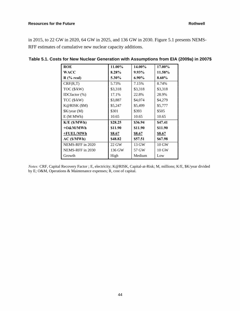
Resources for the Future Rothwell
44
in 2015, to 22 GW in 2020, 64 GW in 2025, and 136 GW in 2030. Figure 5.1 presents NEMS-RFF estimates of cumulative new nuclear capacity additions.
Table 5.1. Costs for New Nuclear Generation with Assumptions from EIA (2009a) in 2007$
ROE 11.00% 14.00% 17.00% WACC 8.28% 9.93% 11.58% R (% real) 5.30% 6.90% 8.60% CRF(R,T) 5.73% 7.15% 8.74% TOC ($/kW) $3,318 $3,318 $3,318 IDCfactor (%) 17.1% 22.8% 28.9% TCC ($/kW) $3,887 $4,074 $4,279 K@RISK ($M) $5,247 $5,499 $5,777 $K/year (M) $301 $393 $505 E (M MWh) 10.65 10.65 10.65 K/E ($/MWh) $28.25 $36.94 $47.41 +O&M/MWh $11.90 $11.90 $11.90 +FUEL/MWh $8.67 $8.67 $8.67 AC ($/MWh) $48.82 $57.51 $67.98 NEMS-RFF in 2020 22 GW 13 GW 10 GW NEMS-RFF in 2030 136 GW 57 GW 10 GW Growth High Medium Low
Notes: CRF, Capital Recovery Factor ; E, electricity; K@RISK, Capital-at-Risk; M, millions; K/E, $K/year divided by E; O&M, Operations & Maintenance expenses; R, cost of capital.

Resources for the Future Rothwell
45
Figure 5.1. Comparing Cumulative New Nuclear Capacity across Scenarios
01224364860728496
108120132144
2010 2015 2020 2025 2030
New
GW
Core-1_11%
Core-1_14%
Core-2nCore-2
Core-1
Table 5.2. Core 1—Nuclear ROE Reduced to 14 Percent Nominal Carbon and Electricity Results NEMS Run: core1_nukroe14.d080309a
% change from % change from % change from % change from2015 Core 1 2020 Core 1 2025 Core 1 2030 Core 1
Carbon Dioxide Emissions (mmtCO2e)Electricity 2,380 0% 2,433 -1% 2,469 -2% 2,468 -7%
Delivered Energy Prices (2007$)Average Electricity Price (cents per KWh) $8.69 0% $9.28 0% $9.44 0% $9.69 -4%Average Natural Gas Price ($ per mcf) $8.28 0% $9.35 -2% $9.17 -3% $10.17 -5%
Average Coal Price ($ per short ton) $39.41 0% $40.02 0% $40.20 0% $40.46 -2%
Electric Capacity by Fuel/Tech (GW)Conventional Coal (PC Boilers) 324 0% 324 0% 324 0% 326 -1%Conventional Gas/Oil (Steam) 93 0% 93 0% 93 0% 92 -1%Conventional Gas/Oil (Combined Cycle) 196 0% 196 0% 210 -4% 219 -7%Combustion Turbine/Diesel 131 -2% 135 -4% 155 -4% 184 -2%Renewables/Other 178 1% 178 1% 182 1% 183 1%Nuclear 104 0% 117 6% 127 15% 157 42%New Nuclear Capacity from Core 1 1.18 0% 12.86 101% 23 2.64 57 4.40Total Capacity (Power Sector) 1,028 0% 1,047 0% 1,095 0% 1,165 2%
Notes: mcf, million cubic feet; Mt, million tonnes; CO2e, CO2 emissions, t-CO2, tonnes of CO2.
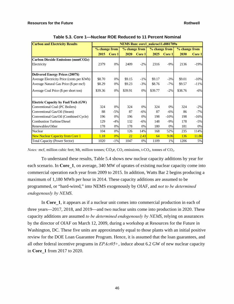
Resources for the Future Rothwell
46
Table 5.3. Core 1—Nuclear ROE Reduced to 11 Percent Nominal Carbon and Electricity Results NEMS Run: core1_nukroe11.d081709a
% change from % change from % change from % change from2015 Core 1 2020 Core 1 2025 Core 1 2030 Core 1
Carbon Dioxide Emissions (mmtCO2e)Electricity 2379 0% 2409 -2% 2316 -9% 2136 -19%
Delivered Energy Prices (2007$)Average Electricity Price (cents per KWh) $8.70 0% $9.15 -1% $9.17 -3% $9.01 -10%Average Natural Gas Price ($ per mcf) $8.29 0% $9.23 -3% $8.76 -7% $9.57 -11%
Average Coal Price ($ per short ton) $39.36 0% $39.91 0% $39.77 -2% $38.76 -6%
Electric Capacity by Fuel/Tech (GW)Conventional Coal (PC Boilers) 324 0% 324 0% 324 0% 324 -2%Conventional Gas/Oil (Steam) 88 -5% 87 -6% 87 -6% 86 -7%Conventional Gas/Oil (Combined Cycle) 196 0% 196 0% 198 -10% 198 -16%Combustion Turbine/Diesel 129 -4% 132 -6% 148 -9% 178 -5%Renewables/Other 178 0% 178 0% 180 0% 181 0%Nuclear 104 0% 126 14% 168 52% 235 114%New Nuclear Capacity from Core 1 1.18 0% 22 2.43 64 9.06 136 11.86Total Capacity (Power Sector) 1020 -1% 1047 0% 1109 1% 1206 5%
Notes: mcf, million cubic feet; Mt, million tonnes; CO2e, CO2 emissions, t-CO2, tonnes of CO2.
To understand these results, Table 5.4 shows new nuclear capacity additions by year for each scenario. In Core_1, on average, 340 MW of uprates of existing nuclear capacity come into commercial operation each year from 2009 to 2015. In addition, Watts Bar 2 begins producing a maximum of 1,180 MWh per hour in 2014. These capacity additions are assumed to be programmed, or “hard-wired,” into NEMS exogenously by OIAF, and not to be determined endogenously by NEMS.
In Core_1, it appears as if a nuclear unit comes into commercial production in each of three years—2017, 2018, and 2019—and two nuclear units come into production in 2020. These capacity additions are assumed to be determined endogenously by NEMS, relying on assurances by the director of OIAF on March 12, 2009, during a workshop at Resources for the Future in Washington, DC. These five units are approximately equal to those plants with an initial positive review for the DOE Loan Guarantee Program. Hence, it is assumed that the loan guarantees, and all other federal incentive programs in EPAct05+, induce about 6.2 GW of new nuclear capacity in Core_1 from 2017 to 2020.
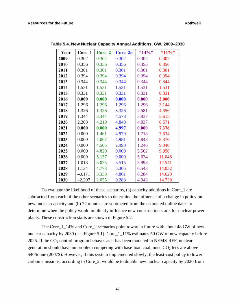
Resources for the Future Rothwell
47
Table 5.4. New Nuclear Capacity Annual Additions, GW, 2009–2030
Year Core_1 Core_2 Core_2n “14%” “11%” 2009 0.302 0.302 0.302 0.302 0.302 2010 0.356 0.356 0.356 0.356 0.356 2011 0.301 0.301 0.301 0.301 0.301 2012 0.394 0.394 0.394 0.394 0.394 2013 0.344 0.344 0.344 0.344 0.344 2014 1.531 1.531 1.531 1.531 1.531 2015 0.331 0.331 0.331 0.331 0.331 2016 0.000 0.000 0.000 0.000 2.000 2017 1.296 1.296 1.296 1.296 3.144 2018 1.326 1.326 3.326 2.581 4.356 2019 1.344 3.344 4.578 3.937 5.615 2020 2.208 4.210 4.840 4.837 6.571 2021 0.000 0.000 4.997 0.000 7.376 2022 0.000 1.461 4.979 1.718 7.634 2023 0.000 4.067 4.981 1.843 8.376 2024 0.000 4.505 2.990 1.246 9.048 2025 0.000 4.820 0.000 5.562 9.956 2026 0.000 5.157 0.000 5.634 11.046 2027 1.013 5.025 3.515 5.998 12.541 2028 1.134 4.773 5.305 6.543 14.052 2029 –0.171 3.338 4.861 6.284 14.629 2030 –2.207 2.055 0.283 4.943 14.738
To evaluate the likelihood of these scenarios, (a) capacity additions in Core_1 are subtracted from each of the other scenarios to determine the influence of a change in policy on new nuclear capacity and (b) 72 months are subtracted from the estimated online dates to determine when the policy would implicitly influence new construction starts for nuclear power plants. These construction starts are shown in Figure 5.2.
The Core_1_14% and Core_2 scenarios point toward a future with about 48 GW of new nuclear capacity by 2030 (see Figure 5.1). Core_1_11% estimates 50 GW of new capacity before 2025. If the CO2 control program behaves as it has been modeled in NEMS-RFF, nuclear generation should have no problem competing with base-load coal, once CO2 fees are above $40/tonne (2007$). However, if this system implemented slowly, the least-cost policy to lower carbon emissions, according to Core_2, would be to double new nuclear capacity by 2020 from
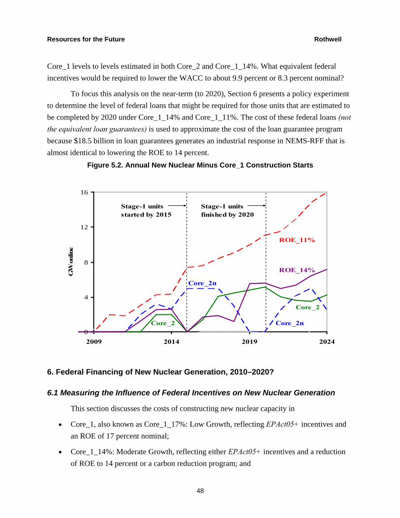
Resources for the Future Rothwell
48
Core_1 levels to levels estimated in both Core_2 and Core_1_14%. What equivalent federal incentives would be required to lower the WACC to about 9.9 percent or 8.3 percent nominal?
To focus this analysis on the near-term (to 2020), Section 6 presents a policy experiment to determine the level of federal loans that might be required for those units that are estimated to be completed by 2020 under Core_1_14% and Core_1_11%. The cost of these federal loans (not the equivalent loan guarantees) is used to approximate the cost of the loan guarantee program because $18.5 billion in loan guarantees generates an industrial response in NEMS-RFF that is almost identical to lowering the ROE to 14 percent.
Figure 5.2. Annual New Nuclear Minus Core_1 Construction Starts
0
4
8
12
16
2009 2014 2019 2024
GW
onl
ine
Stage-1 units finished by 2020
Stage-1 units started by 2015
Core_2n
Core_2
Core_2nCore_2
ROE_11%
ROE_14%
6. Federal Financing of New Nuclear Generation, 2010–2020?
6.1 Measuring the Influence of Federal Incentives on New Nuclear Generation
This section discusses the costs of constructing new nuclear capacity in
• Core_1, also known as Core_1_17%: Low Growth, reflecting EPAct05+ incentives and an ROE of 17 percent nominal;
• Core_1_14%: Moderate Growth, reflecting either EPAct05+ incentives and a reduction of ROE to 14 percent or a carbon reduction program; and
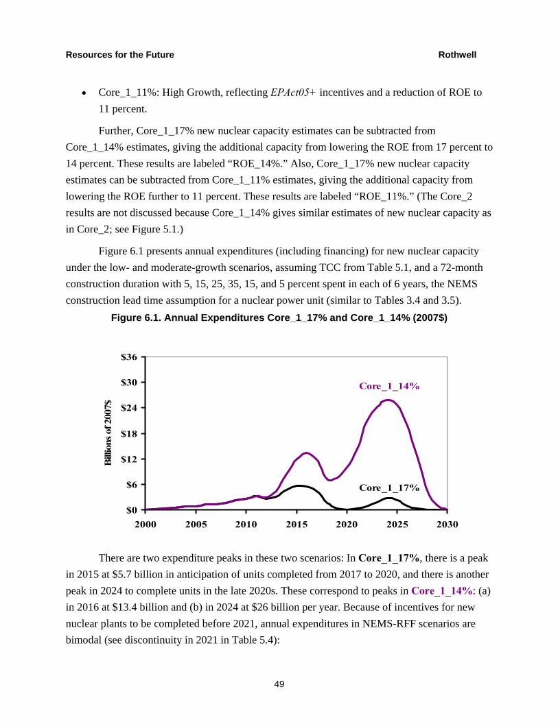
Resources for the Future Rothwell
49
• Core_1_11%: High Growth, reflecting EPAct05+ incentives and a reduction of ROE to 11 percent.
Further, Core_1_17% new nuclear capacity estimates can be subtracted from Core_1_14% estimates, giving the additional capacity from lowering the ROE from 17 percent to 14 percent. These results are labeled “ROE_14%.” Also, Core_1_17% new nuclear capacity estimates can be subtracted from Core_1_11% estimates, giving the additional capacity from lowering the ROE further to 11 percent. These results are labeled “ROE_11%.” (The Core_2 results are not discussed because Core_1_14% gives similar estimates of new nuclear capacity as in Core_2; see Figure 5.1.)
Figure 6.1 presents annual expenditures (including financing) for new nuclear capacity under the low- and moderate-growth scenarios, assuming TCC from Table 5.1, and a 72-month construction duration with 5, 15, 25, 35, 15, and 5 percent spent in each of 6 years, the NEMS construction lead time assumption for a nuclear power unit (similar to Tables 3.4 and 3.5).
Figure 6.1. Annual Expenditures Core_1_17% and Core_1_14% (2007$)
$0
$6
$12
$18
$24
$30
$36
2000 2005 2010 2015 2020 2025 2030
Bill
ions
of 2
007$
Core_1_14%
Core_1_17%
There are two expenditure peaks in these two scenarios: In Core_1_17%, there is a peak in 2015 at $5.7 billion in anticipation of units completed from 2017 to 2020, and there is another peak in 2024 to complete units in the late 2020s. These correspond to peaks in Core_1_14%: (a) in 2016 at $13.4 billion and (b) in 2024 at $26 billion per year. Because of incentives for new nuclear plants to be completed before 2021, annual expenditures in NEMS-RFF scenarios are bimodal (see discontinuity in 2021 in Table 5.4):

Resources for the Future Rothwell
50
1. stage-1 (or first wave) are those plants scheduled to be completed between 2017 and 2021 (i.e., the set of units started after 2012, so-called Generation III reactors, which does not include the TVA completion of Watts Bar 2, a PWR, which is Generation II technology) and
2. stage-2 plants (or second wave) to be completed from 2021 to 2030.
To understand the underlying financing of these deployment scenarios, Figure 6.2 presents the same information as Figure 6.1 but shows annual expenditures for only 2010 to 2020. These expenditures have been translated into 2010 to 2020 nominal dollars, assuming a 3 percent inflation rate. Figure 6.2 shows annual expenditures for
• Core_1: with 6.2 GW, Core_1_17% also includes 4 GW of Generation II plants and uprates before 2017;
• ROE_14%: with an added 6.5 GW above Core_1 for a 12.7-GW total; and
• ROE_11%: with an added 17.3 GW above Core_1 for a 23.5-GW total.
Figure 6.2. Stage 1 Annual Expenditures in Escalated 2010 to 2020 Dollars
$0
$6
$12
$18
$24
$30
$36
2010 2011 2012 2013 2014 2015 2016 2017 2018 2019 2020
Bill
ions
Core_1
ROE_14%
ROE_11%
Figure 6.2 shows that the influence of the EPAct05+ incentives is similar to lowering the ROE to 14 percent: they both induce a little more than 6 GW of new nuclear capacity. The spending profiles for Core_1 with 6.2 GW and ROE_14% with a marginal 6.5 GW are very similar. This could be because both sets of policies have a similar effect on the cost of capital, a very sensitive parameter in NEMS, as shown in Section 5. If DOE were to double the size of the

Resources for the Future Rothwell
51
Loan Guarantee Program, new nuclear capacity could be similar to Core_1_14% (= Core_1+ROE_14%).
Regarding the financing of Stage-2, if Core_2 results are correct, there should be no need for federal incentives to encourage nuclear generation in Stage-2 under an effective carbon control program. The focus of current DOE nuclear generation policy (following this policy analysis) should be on (a) stewarding Stage-1 plants into production to provide an alternative non-carbon generating technology, and (b) encouraging an effective carbon control regime.
Although Core_1 estimates only 6.2 GW of new nuclear capacity, to cover these units (at 80 percent of their TCC), total eligible debt would be above the $18.5 billion limit. The Obama administration has proposed increasing the limit to $54 billion. What are the costs and benefits of increasing the current level of loan guarantees to the new nuclear generators?
6.2 Measuring the Cost of Federal Incentives to Encourage New Nuclear Generation
To calculate the costs of a hypothetical federal financial incentive program, consider a policy experiment with three financial instruments:
• private equity, requiring a nominal rate of return of 17, 14, or 11 percent;
• private debt, with a nominal 8 percent rate of interest; and
• public debt, with a nominal 0 percent rate of interest (although this form of debt is not available, it is used as a simple construct for calculating the cost to the public of subsidizing new nuclear capacity).
Assuming a nominal ROE of 14 percent, if financing were done through a combination of 45 percent equity, 45 percent private debt, and 10 percent public debt, the nominal WACC would be 9.88 percent (or about 9.93 percent, as in Table 5.1).
With a nominal ROE of 11 percent, if financing were done through a combination of 37.5 percent equity, 37.5 percent private debt, and 25 percent public debt, the nominal WACC would be 8.21 percent (or about 8.28 percent, as in Table 5.1). What would be the cost of this public debt?
If the private capital market would have charged 8 percent nominal on debt, then the opportunity cost of providing federal funding at 0 percent nominal is 8 percent nominal (or about 5 percent real). And assuming that the (unpaid) interest begins accruing in 2020, Table 6.1 presents the opportunity cost to the U.S. government of encouraging more nuclear power plant
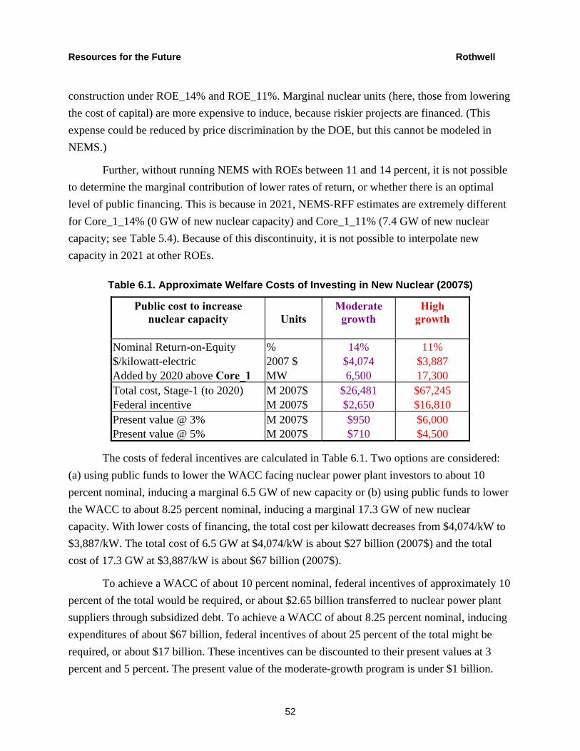
Resources for the Future Rothwell
52
construction under ROE_14% and ROE_11%. Marginal nuclear units (here, those from lowering the cost of capital) are more expensive to induce, because riskier projects are financed. (This expense could be reduced by price discrimination by the DOE, but this cannot be modeled in NEMS.)
Further, without running NEMS with ROEs between 11 and 14 percent, it is not possible to determine the marginal contribution of lower rates of return, or whether there is an optimal level of public financing. This is because in 2021, NEMS-RFF estimates are extremely different for Core_1_14% (0 GW of new nuclear capacity) and Core_1_11% (7.4 GW of new nuclear capacity; see Table 5.4). Because of this discontinuity, it is not possible to interpolate new capacity in 2021 at other ROEs.
Table 6.1. Approximate Welfare Costs of Investing in New Nuclear (2007$)
Public cost to increase nuclear capacity Units
Moderate growth
High growth
Nominal Return-on-Equity % 14% 11% $/kilowatt-electric 2007 $ $4,074 $3,887 Added by 2020 above Core_1 MW 6,500 17,300 Total cost, Stage-1 (to 2020) M 2007$ $26,481 $67,245 Federal incentive M 2007$ $2,650 $16,810 Present value @ 3% M 2007$ $950 $6,000 Present value @ 5% M 2007$ $710 $4,500
The costs of federal incentives are calculated in Table 6.1. Two options are considered: (a) using public funds to lower the WACC facing nuclear power plant investors to about 10 percent nominal, inducing a marginal 6.5 GW of new capacity or (b) using public funds to lower the WACC to about 8.25 percent nominal, inducing a marginal 17.3 GW of new nuclear capacity. With lower costs of financing, the total cost per kilowatt decreases from $4,074/kW to $3,887/kW. The total cost of 6.5 GW at $4,074/kW is about $27 billion (2007$) and the total cost of 17.3 GW at $3,887/kW is about $67 billion (2007$).
To achieve a WACC of about 10 percent nominal, federal incentives of approximately 10 percent of the total would be required, or about $2.65 billion transferred to nuclear power plant suppliers through subsidized debt. To achieve a WACC of about 8.25 percent nominal, inducing expenditures of about $67 billion, federal incentives of about 25 percent of the total might be required, or about $17 billion. These incentives can be discounted to their present values at 3 percent and 5 percent. The present value of the moderate-growth program is under $1 billion.
Resources for the Future Rothwell
53
The present value of the high-growth program is between $4.5 billion and $6 billion. These are higher than the CBO estimates discussed in Section 2.3, which could be from the inability to price discriminate among investors in this analysis. In other words, CBO assumes that the loan guarantee fees will match the risk status of the investor, but this cannot be modeled in NEMS because NEMS treats all investors as identically and independently risky. So the cost to the public calculated here could be upwardly biased.
But could reactor vendors produce another 6.5 to 17.3 GW by 2020? The ability of reactor vendors to complete their orders before 2020 is a function of their optimal level of orders: because of the high fixed costs of entering the market, a low level of orders (e.g., one per year) is not sustainable; simultaneously, a high level of orders (e.g., one per month) might not be sustainable either. So each reactor vendor has an optimal level (e.g., between one per month and one per year).
To date, new nuclear power plant investors have selected the AP1000a as the strongest competitor. Of the 16.5 GW expected to be completed by 2020, 74 percent is on order from Toshiba-Westinghouse-Shaw, 16 percent is on order from General Electric-Hitachi, and 10 percent is on order from France’s AREVA. Although the two ABWRs and the one U.S. EPR have been given preliminary positive reviews for loan guarantees, it is unlikely that orders for only one or two reactors will be profitable for a reactor vendor. Of course, the ABWRs are similar to those in Japan (see Figure 3.1), so some experience can be transferred. And the U.S. EPR is similar to EPRs in Finland and France, so some experience can be transferred (but the French experience to date points toward costs for the EPR that are higher than those now expected).
If a real competitor to the AP1000a is to be found before the loan guarantees are fully allocated, there should be a minimum number of units with EPC orders (e.g., at two sites) before a loan guarantee is granted. This is because single-plant projects are more likely to be over schedule and over budget than multiple-site projects because of the lack of economies of series in production. Not allocating all of the loan guarantees under a “minimum number of orders” policy would insure that funds will be available later for a stronger competitor to the AP1000a.
If no other competitor emerges, could Toshiba-Westinghouse-Shaw construct 16 GW by 2020 (two per year from 2012), then 32 GW by 2030 (three per year)? Westinghouse produced this much capacity from 1965 to 1985. So this appears feasible, but the COL for the AP1000a has not yet been granted, so the construction start dates are still uncertain.
Resources for the Future Rothwell
54
Under the high-growth scenario, with only one standardized design (following the French model of the 1970s and 1980s), could a single vendor construct 24 GW by 2020 (3 per year from 2012), another 40 GW (8 per year) in five years, and another 70 GW in another five years (14 per year)? This is unlikely for a single firm or group of firms. Nor is this scenario likely with more than one Nuclear Steam System Supplier.
If 32 GW can be built between 2020 and 2030, it is likely that new nuclear capacity could double again by 64 GW from 2030 to 2040 (at the rate of six units per year). This would allow 112 GW of Generation III nuclear capacity to replace retiring Generation II capacity, just as Generation IV designs (e.g., fast reactors) enter the market.
Marginal nuclear units require higher levels of public capital incentives, primarily because riskier projects are being subsidized. At some level of deployment, the probability that at least one nuclear project would default on a loan guarantee increases. When one borrower defaults, risk premiums could rise for other projects, which in turn could cause further defaults. To maximize the probability of orders after 2020, this should be avoided. Thus, in determining the optimal deployment level of new nuclear capacity in the United States, there is a trade-off between more projects and higher default risk on loan guarantees. Because of this, the optimal level of loan guarantees is not obvious.
6.3 Measuring the Benefits of Federal Incentives for New Nuclear Generation
To compare the public’s costs of encouraging nuclear generation with the public’s benefits, two benefits are considered: (a) the reduction in petroleum consumption in millions of barrels (mmb) and (b) the reduction in energy sector–related CO2 emissions in mmt. Table 6.2 presents these metrics.
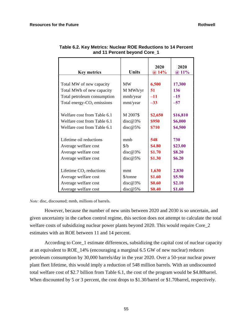
Resources for the Future Rothwell
55
Table 6.2. Key Metrics: Nuclear ROE Reductions to 14 Percent and 11 Percent beyond Core_1
Key metrics Units 2020
@ 14% 2020
@ 11% Total MW of new capacity MW 6,500 17,300 Total MWh of new capacity M MWh/yr 51 136 Total petroleum consumption mmb/year –11 –15 Total energy-CO2 emissions mmt/year –33 –57 Welfare cost from Table 6.1 M 2007$ $2,650 $16,810 Welfare cost from Table 6.1 disc@3% $950 $6,000 Welfare cost from Table 6.1 disc@5% $710 $4,500 Lifetime oil reductions mmb 548 730 Average welfare cost $/b $4.80 $23.00 Average welfare cost disc@3% $1.70 $8.20 Average welfare cost disc@5% $1.30 $6.20 Lifetime CO2 reductions mmt 1,630 2,830 Average welfare cost $/tonne $1.60 $5.90 Average welfare cost disc@3% $0.60 $2.10 Average welfare cost disc@5% $0.40 $1.60
Note: disc, discounted; mmb, millions of barrels.
However, because the number of new units between 2020 and 2030 is so uncertain, and given uncertainty in the carbon control regime, this section does not attempt to calculate the total welfare costs of subsidizing nuclear power plants beyond 2020. This would require Core_2 estimates with an ROE between 11 and 14 percent.
According to Core_1 estimate differences, subsidizing the capital cost of nuclear capacity at an equivalent to ROE_14% (encouraging a marginal 6.5 GW of new nuclear) reduces petroleum consumption by 30,000 barrels/day in the year 2020. Over a 50-year nuclear power plant fleet lifetime, this would imply a reduction of 548 million barrels. With an undiscounted total welfare cost of $2.7 billion from Table 6.1, the cost of the program would be $4.80barrel. When discounted by 5 or 3 percent, the cost drops to $1.30/barrel or $1.70barrel, respectively.
Resources for the Future Rothwell
56
Also, subsidizing the capital cost of nuclear capacity at equivalent to ROE_11% (encouraging a marginal 17.3 GW of new nuclear) reduces petroleum consumption by 40,000 barrels/day in the year 2020. Here, tripling nuclear capacity in NEMS-RFF decreases petroleum consumption by only one-third, which does not seem reasonable. Over the 50-year lifetime, this would imply a reduction of 730 million barrels. With an undiscounted total welfare cost of $17 billion from Table 6.1, the cost of the program would be $23/barrel. When discounted, the cost is between $6.16/barrel and $8.21/barrel.
Regarding CO2 reductions, according to Core_1 differences, subsidizing the capital construction cost of nuclear at an equivalent to ROE_14%—that is, encouraging 6.5 GW of new nuclear—reduces CO2 in the energy sector by 33 mmt of CO2 per year in the year 2020. Over a 50-year lifetime, this would be 1,630 mmt. Is this reasonable?
The results in Table 6.2 can be compared to the amounts of CO2 that equivalent capacities of natural gas (using Combined-Cycle Gas Turbine, CCGT) and coal would produce. With a carbon intensity factor of 0.52 t-CO2/MWh (tonnes of CO2 per MWh), 6.5 GW of CCGT would produce about 27 mmt per year. With a carbon intensity factor of 0.92 t-CO2/MWh, 6.5 GW of coal would produce about 47 mmt of CO2 per year. Given that new nuclear capacity in ROE_14% is reducing CO2 emissions by 33 mmt (which is between 27 mmt of CO2 emissions for replacing all natural gas and 47 mmt of CO2 emissions for replacing all coal), the NEMS-RFF results are reasonable.
With an undiscounted total welfare cost of $2,650 million, the cost of the program would be $1.63/t-CO2. Discounted costs are between $0.44/t-CO2 and $0.58/t-CO2, and could be as low as $0.30/t-CO2 if nuclear displaces all coal at a discount rate of 5 percent.
Subsidizing the capital construction cost of nuclear at equivalent to ROE_11%—that is, encouraging 17.3 GW of new nuclear by 2020—reduces CO2 in the energy sector by only 57 mmt in the year 2020. Over a 50-year nuclear power plant fleet lifetime, this would imply an equivalent of 2,830 mmt of CO2. This can be compared with the amounts of CO2 that equivalent capacities of CCGT and coal would produce: 17.3 GW of CCGT would produce about 72 mmt per year, and 17.3 GW of coal would produce about 125 mmt per year. For example, if 6.5 GW reduces CO2 by 33 mmt, then 17.3 GW should reduce CO2 by at least 88 mmt in 2020, or 50 percent more than projected by NEMS-RFF. With an undiscounted total welfare cost of $17 billion, the cost of the program would be $5.94/t-CO2, and discounted costs would be between $1.59/t-CO2 and $2.12/t-CO2.
Resources for the Future Rothwell
57
Reductions in CO2 emissions could justify increasing incentives to nuclear generation through 2020 as a function of the competing alternative average welfare costs per tonne of CO2. New nuclear capacity replacing coal is one of the most cost-effective carbon control strategies (given the lack of a more effective carbon control regime). After 2020, the electric utility industry will have a better understanding of the costs, risks, benefits, and revenues from new nuclear capacity and any new carbon control regime. Assessing the costs and benefits of subsidizing the nuclear generation industry beyond 2020 is hindered by too many uncertainties at this time.
Until an effective carbon control regime is established, it is easy to conclude that both the moderate-growth (about 16 GW by 2020) and high-growth (about 24 GW by 2020) scenarios yield tremendous reductions in CO2 emissions per dollar spent in federal incentives.
7. Whither Irradiated Fuel?
The sustainability of nuclear power depends on other issues beyond economic competitiveness and whether the LWR industry can grow. Rothwell and Van der Zwaan (2003, 70) propose criteria (compare to Rogner 2001) for the intermediate sustainability of an energy system (where intermediate sustainability allows some substitution between natural resources and other inputs, such as capital):
1. Nonrenewable resource depletion: Does the energy system rely on fuels or materials that could be depleted . . .?
2. Environmental externalities: Do emissions from the energy system accumulate faster than the absorption capacity of the environment?
3. Social externalities: Does the energy system impose externalities on populations (current or future) . . .?
Regarding the first criterion, Rothwell and Van der Zwann (2003) conclude that LWR energy systems are not sustainable because of their fuel inefficiency for more than a few centuries: Uranium-235 is a depletable resource and some of this depletable resource is discarded with the used fuel. However, to greatly increase fuel efficiency requires reprocessing used fuel, which can impose social externalities (e.g., proliferation risks), thus undermining LWR sustainability.
These issues are also tied to the second criterion: can the environment safely absorb, or sequester, the waste products from LWR energy systems? Section 7.1 compares the cost of
Resources for the Future Rothwell
58
sequestering irradiated fuel with the cost of sequestering CO2, and finds that the total cost of sequestering CO2 from a fossil-fired power plant could be many times greater than the cost of sequestering irradiated fuel from an equal-sized nuclear power plant. Section 7.2 explores the costs and uncertainties of the alternatives available to manage this irradiated fuel. Section 7.3 discusses how these issues might slow the licensing of new nuclear power plants, given the DOE decision to withdraw its license application for the Yucca Mountain repository.
This section will not address other perceived, or misperceived, social externalities associated with nuclear power. For example, the issue of nuclear power plant safety has been largely resolved with the implementation of a “safety culture” in the U.S. nuclear power industry. The industry has had an excellent industrial safety record (particularly when compared to safety records in the coal and oil industries). In countries without a strong safety culture, as in late-Soviet Ukraine, a non-negligible probability remains of an accidental off-site radioactive release. However, it is unlikely that the issue of potential catastrophic accidents at Generation III nuclear power plants or proliferation will influence new construction in the United States (although these issues could influence new nuclear construction in other countries). Although safety questions could arise, the issue of plant health and safety is much less significant than the issues of cost (addressed in Sections 2–6) and irradiated fuel (addressed in this section).
7.1 Sequestering New Nuclear Power’s Used Fuel or Fossil Fuel’s CO2?
To place the issue of irradiated fuel management in context, one must compare it to the problem of carbon capture and storage (CCS). Consider that 1,000 MWe of nuclear capacity generates about 20 MTHM per year (assuming 50 MW-thermal-days/kg of uranium), and that 1,000 MWe of coal generates about 7,230,000 tonnes of CO2 per year. During the year, the nuclear power plant owner is taxed $8 million for the future sequestration of the 20 tonnes of Spent Nuclear Fuel (SNF; the term SNF is used because it is the term used in the Nuclear Waste Policy Act of 1982, as amended, NWPA+). A coal plant of equal size pays nothing for the CO2 it emits.
The cost of sequestering CO2 could be at least $10/tonne, about $72 million per year, or almost 10 times greater than SNF sequestration. Because of the lack of large-scale CO2 sequestration sites, it is not known how high these costs could be. In particular, OIAF (2009, 6) notes “[t]here is great uncertainty about how fast these technologies, the industries that support them, and the regulatory infrastructure that licenses/permits them might be able to grow and, for fossil with CCS when the technology will be fully commercialized.” Of course, the cost for disposing of SNF could also be higher. However, much more experience has been gained with
Resources for the Future Rothwell
59
SNF sequestration costs; in fact, national SNF sequestration programs are under way in Europe. But even with uncertain nuclear sequestration costs, their impact on total generation cost is better understood than the unknown impact of CO2 sequestration on fossil-fired electricity costs.
7.2 What are the Costs and Uncertainties of U.S. SNF Alternatives?1
The three sets of alternatives for managing LWR SNF have been identified as: Alternative (A) once-through uranium oxide fuel cycle with temporary storage and geologic repository disposal; Alternative (B) twice-through reprocessing with fabrication of mixed oxide (MOX) fuel for LWRs; and Alternative (C) full recycling of actinides (plutonium and others) in Fast-Burner or Breeder Reactors (FBRs). After much debate, the U.S. Congress chose Alternative (A) as the best option in the passage of the NWPA+. Thus, proponents of Alternatives (B) and (C) must show that these options are better than Alternative (A).2
However, in all scenarios, a geologic repository is required, given legacy SNF and DOE high-level (radioactive) waste. So the first determination is not whether to store SNF and build a geologic repository, but how to employ geologic repository capacity most efficiently. In other words, the first step is to determine the level of SNF processing that is most efficient given U.S. resources and repository capacity constraints.
Given that Alternative (A) is U.S. policy, if it is determined that reprocessing should begin as soon as possible to more efficiently deploy future repository capacity, then Alternative (B) is the only immediate option, because Alternative (C) will not be available for decades. If it is determined that repository capacity must be minimized, then Alternative (C) is the only option, because Alternative (B) cannot burn actinides as efficiently as Alternative (C). A portfolio of all three alternatives could be the least risky strategy, but deploying all three might be too costly.
1 Section 7.2 is based on text in a forthcoming report by the Johns Hopkins University, Global Energy and Environment Initiative, Policy Review Panel on Reprocessing and Recycling Spent Nuclear Fuel. 2 Given that no repository site is under consideration, to facilitate interim storage, Congress should strike the
following language in the NWPA: “Sec. 148 (d) Licensing conditions. Any license issued by the NRC for a Monitored Retrievable Storage facility under this section shall provide that – (1) construction of such facility may not begin until the NRC has issued a license for the construction of a repository under section 115(d); (2) construction of such facility . . . shall be prohibited during such time as . . . construction of the repository ceases; (3) the quantity of SNF or high-level radioactive waste (HLW) at the site of such facility at any one time may not exceed 10,000 MTHM until a repository under this Act first accepts SNF or solidified HLW; and (4) the quantity of SNF or HLW at the site of such facility at any one time may not exceed 15,000 MTHM.” (emphasis added.)
Resources for the Future Rothwell
60
During the past decade, numerous economic and cost-engineering studies have attempted to estimate the lifecycle costs of these SNF alternatives. For a review of these studies, including the Boston Consulting Group (2006) report for AREVA, see De Roo and Parsons (2009). But few of these studies identify financial risks and uncertainties associated with each alternative. For example, under all alternatives, a repository is required for all (under once-through) or some (with reprocessing) of the SNF. But the cost of ultimate disposal is uncertain, particularly if the Yucca Mountain repository is not built. Fortunately, because of the extensive characterization of the repository, the cost of ultimate disposal can be parameterized as a cost per megawatt-hour ($/MWh) with an asymmetric probability distribution.
Regarding Alternative (C), the cost of FBRs and their fuel is unknown. Many studies assume a 20 percent cost difference between LWRs and FBRs; this ignores the FBR first-of-a-kind costs, which could be twice as much as Nth-of-a-kind LWR costs (implying high subsidies to equalize the LUEC between commercial LWR and FBR power plants). For example, see De Roo and Parsons (2009, 30): “[w]e assume that the fast reactor capital and operating costs are 20% higher than the comparable costs for the light water reactor.” This assumption is discussed by Idaho National Laboratory (2009, R2-9),
A commonly heard “rule-of-thumb” is that the fast reactor will be 20% higher than a LWR on a per kilowatt of capital basis. Russian experience has shown this factor to be more like 60% . . . These cost comparisons are currently speculative. . . .
The crucial (and as yet unknown) parameters in calculating the cost of full recycle are (a) the burnup rate in future FBRs (the planned Japanese fast reactor program assumes a breeding rate of 2 percent to produce plutonium for fast-reactor MOX) and (b) the cost of qualifying fuels of various actinide compositions as the actinides are burned completely, thus, theoretically, eliminating the need for more than one geologic repository. However, given that the cost of MOX fuel fabrication has been rising (primarily from tighter health, safety, and environmental standards), the cost of fabricating FBR fuels in hot cells with various levels of actinides is high and its probability distribution is unknown. Thus, the estimated costs of full recycling with the associated fast-reactor nuclear energy systems are speculative.
No existing deterministic cost study of full recycling is credible because there has been no engineering demonstration of full recycling. There is no debate that electricity from FBRs will be more expensive than electricity from LWRs. There is no debate that remote reprocessing and fabrication of recycled fuel, as required by all technologies in Alternative (C) will be more expensive than reprocessing LWR used fuel for MOX fabrication (Rothwell 2009b). One can
Resources for the Future Rothwell
61
reasonably conclude that full recycling in FBRs, Alternative (C), is the most expensive alternative (although it is not known how much more expensive it might be, or whether these costs could be completely offset by reduced uranium costs and waste disposal savings).
Also, regarding Alternatives (B) and (C), most proponents of reprocessing assume that a government will pay for everything. But if Alternative (B) is not competitive at market costs of capital, and must rely completely on government funding, then Alternative (B) is not ready for commercial deployment in the United States. Bunn et al. (2003) show that Alternative (B) might not be competitive for the United States until the price of uranium rises above its historic highs (Rothwell 1980) or the cost of final disposal is shown to be much greater than the estimated cost of completing the Yucca Mountain repository (Office of Civilian Radioactive Waste Management 2008).
On the other hand, the costs of storage at centralized facilities are low enough (Rothwell 2010a) that the U.S. government could rely on centralized storage to provide time to solve the SNF problem scientifically, technically, economically, and equitably in anticipation of Generation II nuclear power plant retirements (gradually to 2030, then more quickly after 2030), requiring the removal of all SNF with decommissioning.
Given this, the most effective action that the U.S. government can currently undertake is defining, identifying, and siting at least one geologic repository in the United States, which will be required under all plausible futures. The decision on whether to reprocess should be made after a geologic repository has been sited, so that its space can be most efficiently allocated. But the decision to site a geologic repository must be made now, given the withdrawal of the Yucca Mountain license application. Inaction could leave a permanent scar on the Obama energy policy legacy, and could permanently scare nuclear investors.
7.3 Is There Confidence in the “Waste Confidence Rule”?
Although the question of when to begin reprocessing and what technology to use can be made by future administrations, the Obama administration must propose an appropriate policy response to its decision to withdraw the license application for Yucca Mountain. If it does not, the NRC’s untested licensing process could unravel. Determining an appropriate response is wrapped in the mystery of how to license new nuclear power plants under ever-shifting U.S. government SNF management policy.
The mystery is how to license plants in a new three-part licensing process (ESP, Design Certification, and COL). No nuclear power plant has been licensed under this new system. The
Resources for the Future Rothwell
62
completion of Watts Bar 2 is under the old two-part licensing system (part one is a permit to build a specific design, and part two is a license to operate a specific plant). The hope was that this new process would ease the licensing of nuclear power plants.
However, no certified design has ever been ordered, and no design that has been ordered is certified. There was early optimism that electric utilities would apply early for ESPs (under which the environmental permitting for a generic nuclear power plant would have been approved). But most electric utilities did not apply for ESPs, and half of those that have been approved have been banked for future use. Of the proposed reactor sites in Table 2.2, ESP applications were submitted and approved only for North Anna in Virginia and Vogtle in Georgia. Given that the license application for Yucca Mountain has been withdrawn, the storage of used fuel on the reactor site, as is done now, could become a contentious environmental issue.
The implications of abandoning Yucca Mountain can be seen in “re Dominion Nuclear North Anna,” 60 N.R.C. 253, 2004, as discussed in Lewis (2006). In challenging the ESP for North Anna, the Blue Ridge Environmental Defense League, the Nuclear Information and Resource Service, and Public Citizen made nine contentions. A panel of NRC administrative law judges dismissed seven of these contentions. One of these dismissed contentions was that the ESP application did not address the issue of indefinitely storing SNF at the North Anna site. The administrative ruling dismissed this contention based on the NRC’s “Waste Confidence Rule,” 10 CFR 51.23:
(a) The Commission has made a generic determination that, if necessary, spent fuel generated in any reactor can be stored safely and without significant environmental impacts for at least 30 years beyond the licensed life for operation (which may include the term of a revised or renewed license) of that reactor at its spent fuel storage basin or at either onsite or offsite independent spent fuel storage installations. Further, the Commission believes there is reasonable assurance that at least one mined geologic repository will be available within the first quarter of the twenty-first century, and sufficient repository capacity will be available within 30 years beyond the licensed life for operation of any reactor to dispose of the commercial high-level waste and spent fuel originating in such reactor and generated up to that time.
(b) Accordingly, . . . no discussion of any environmental impact of spent fuel storage in reactor facility storage pools . . . is required in any environmental report, environmental impact statement, environmental assessment, or other analysis prepared in connection with the issuance or amendment of an operating license for a nuclear power reactor under parts 50 and 54 of this chapter, or
Resources for the Future Rothwell
63
issuance or amendment of a combined license for a nuclear power reactor under parts 52 and 54 of this chapter . . . . (emphasis added)
In November 2009, two of the three remaining NRC Commissioners refused to approve an update to the Waste Confidence Rule in response to withdrawing the license application for the Yucca Mountain repository. On March 9, 2010, one of these commissioners, Commissioner Dale Klein, commented on this rule:
Now that one can ask whether the nation is back to square one with regard to the back end of the fuel cycle, the NRC naturally faces the issue of waste confidence. . . . What many people—even many people in this room—fail to understand is that the waste confidence rule is a real challenge for us because it is not simply based on the technical judgment of the NRC. Part of the Commission’s “confidence” underlying the rule must be based on events that are beyond the NRC’s control, and when those events are in flux, the Commission has to be very careful in deciding whether it can credibly say that we have “confidence” that a repository will be open on a given date or period of time.
Although the NRC could focus on the lack of a repository in not renewing its Waste Confidence Rule, it is just as likely that three out of five Commissioners could find that independent spent fuel storage installations (or Monitored Retrievable Storage sites in NWPA+) could be available within a reasonable time after any reactor is built at an ESP site, given that such a storage site was licensed by the NRC in 2006 (Rothwell 2010b). (This could simply require striking the last sentence of 10 CFR 51.23a and voting to update the rule.)
But updating the Waste Confidence Rule might politically require waiting for the findings of the Blue Ribbon Commission (BRC), as DOE is doing. The members of the BRC have 18 months from March 2010 to draft a report for Energy Secretary Chu, and another 6 months to finalize it (by early 2012, although their charter could be extended); the report must address all of the following issues (DOE 2010, 1-2):
(a) Evaluation of existing fuel cycle technologies and R&D programs. Criteria for evaluation should include cost, safety, resource utilization and sustainability, and the promotion of nuclear nonproliferation and counter-terrorism goals;
(b) Options for safe storage of used nuclear fuel while final disposition pathways are selected and deployed;
(c) Options for permanent disposal of used fuel and/or high-level nuclear waste, including deep geological disposal;
(d) Options to make legal and commercial arrangements for the management of used nuclear fuel and nuclear waste in a manner that takes the current and potential full fuel cycles into account;
Resources for the Future Rothwell
64
(e) Options for decision-making processes for management and disposal that are flexible, adaptive, and responsive;
(f) Options to ensure that decisions on management of used nuclear fuel and nuclear waste are open and transparent, with broad participation;
(g) The possible need for additional legislation or amendments to existing laws, including the Nuclear Waste Policy Act of 1982, as amended; and
(h) Any such additional matters as the Secretary determines to be appropriate for consideration.
The political puzzle becomes whether the NRC should (a) vote soon to update the Waste Confidence Rule, (b) wait for the BRC to make recommendations to the Secretary of Energy, or (c) wait until Congress enacts legislation to rectify the current violations of the NWPA+. (If the BRC report is released late in the 112th Congress, it is unlikely that it will have an impact on legislation until the 113th Congress.) Until the NRC updates the Waste Confidence Rule, it is unlikely that any site except Vogtle in Georgia will have the necessary permits to break ground before the November 2012 election. COL approval hearings could be protracted by responding to anticipated and unanticipated issues (i.e., issues that should have been resolved during the ESP process) from petitioners holding stakes in the proceedings.
The BRC should focus on addressing (a) those issues on which the NRC must base the update of its Waste Confidence Rule and (b) those issues on which the U.S. Congress could base legislation after the next congressional election. Without immediate attention (in the 112th Congress), new U.S. nuclear generation could get off to a slow start. As observed in The Financial Times,
The Obama administration’s efforts to foster a renaissance in nuclear power in the U.S. are coming up against an old dilemma—what to do with the waste . . . In March 2009, Mr. Obama announced that Yucca Mountain, the country’s only prospective nuclear waste repository, would be shut before ever opening . . . The closure has shaken the nuclear power industry during what some are calling its long-awaited revival. The largest nuclear power company, Exelon, has said it will not construct new plants until progress is made on storage. “This is a major impediment to the development of new nuclear sites,” said John Rowe, Exelon’s chief executive.
The Senate climate bill, sponsored by John Kerry, a Democratic senator from Massachusetts, and Joe Lieberman, an independent senator from Connecticut, increases the existing nuclear loan guarantee programme from $18.5 [billion] to over $50 [billion]. Such a programme could spur the construction of a dozen nuclear plants. But the bill leaves the question of waste storage unanswered . . . In the wake of Yucca’s closure, the Energy Department appointed a [blue
Resources for the Future Rothwell
65
ribbon] commission to address the issue of long-term nuclear storage.” (Sieff 2010, emphasis added)
(Note that John Rowe is a member of the Blue Ribbon Commission.)
Whether the nuclear power industry can expand as quickly as some expect during the next decade could depend on (a) a prompt congressional response to the Obama administration’s request for $54 billion in loan guarantees for new nuclear generation and (b) a prompt Obama administration response to a prompt BRC answer to the “question of waste storage.”
Resources for the Future Rothwell
66
Abbreviations and Acronyms
AACEI Association for the Advancement of Cost Engineering International ABWR Advanced Boiling Water Reactor, first constructed in Japan AC Average Cost, set equal to Levelized Unit Electricity Cost AFUDC Allowance for Funds Used During Construction, similar to IDC AP1000a Advanced Passive Pressurized Water Reactor (amended), 1,117 MW APWR (U.S.) Advanced Power Reactor, 1,700 MW B Billions BASE Base Overnight Construction cost BRC “Blue Ribbon Committee” to advise the U.S. Secretary of Energy BWR Boiling Water Reactor (manufactured in the U. S. by General Electric) CF Capacity Factor is the percentage of maximum output generated in year CO2 Carbon Dioxide COL Combined Construction and Operating License CON Contingency on BASE CRF Capital Recovery Factor CWIP Construction Work in Progress, a regulatory implementation of IDC CXt Construction expenditures in period t DOE U.S. Department of Energy E Energy produced, measured in millions of MWh ECP Electricity Capacity Planning, a submodule of NEMS EIA Energy Information Administration EMWG Economic Modeling Working Group EPAct05+ Energy Policy Act of 2005 (plus appropriations) EPC Engineering, Procurement, and Construction (contract) EPR (U.S.) Evolutionary Power Reactor, 1,600 MW ESBWR Economic Simplified Boiling Water Reactor, 1,560 MW FBR Fast Breeder Reactor or Fast Burner Reactor FUEL Fuel costs per year GW Gigawatt of electric capacity, equal to 1,000 MW, or 1,000,000 kW GWh Gigawatt-hour, 1,000 times MWh H Total generating Hours per year h Total hours in an average year, equal to 365.25 times 24 hours = 8766 IDC Interest During Construction (in $M or $/kWh) IDC% Interest During Construction factor, IDC as a percentage of TOC IEA International Energy Agency ISFSI Independent Spent Fuel Storage Installation

Resources for the Future Rothwell
67
K@RISK Capital at Risk, investment required before revenues are generated kWh Kilowatt-hour LT Lead time, length of the construction duration LUEC Levelized Unit Electricity Cost, also known as “levelized cost” LWR Light Water Reactor (e.g., BWR and PWR) M Millions MAX A plant’s annual net maximum dependable output MOX Mixed-Oxide (uranium oxide plus plutonium oxide) fuel MRS Monitored Retrievable Storage, also known as ISFSI MTHM Metric tons of Heavy Metal (uranium plus heavier elements) MW Megawatt-electric (also represented elsewhere as MWe) MWh Megawatt-hour, 1,000 times kWh NEA Nuclear Energy Agency NEMS National Energy Modeling System NPV Net Present Value NRC U.S. Nuclear Regulatory Commission NRG Developer of South Texas Project Units 3 & 4 NWPA+ Nuclear Waste Policy Act of 1982, with amendments O&M Operation and Maintenance expenses OCRWM Office of Civilian Radioactive Waste Management OECD Organisation for Economic Co-operation and Development OIAF Office of Integrated Analysis and Forecasting of EIA; manages NEMS PU Plutonium (PU+ = Plutonium plus actinides) PWR Pressurized Water Reactor R Discount rate, annual r Discount rate, monthly ROE Return-on-Equity SNF Spent Nuclear Fuel, also known as “used fuel” and “irradiated fuel” SWU Separative Work Unit, a measure of effort to enrich uranium T Economic life of the project t Metric tons or time subscript TCC Total Capital Construction costs, defined as TCIC in EMWG (2007) TOC Total Overnight Construction costs, equal to BASE + CON WACC Weighted Average Cost of Capital (an average of rates on debt and equity) WNO World Nuclear Organization
Resources for the Future Rothwell
68
References
AACEI (Association for the Advancement of Cost Engineering International). 1997. Cost Estimate Classification System—As Applied in Engineering, Procurement, and Construction for the Process Industries. Morgantown, WV: AACEI.
BCG (Boston Consulting Group). 2006. Economic Assessment of Used Nuclear Fuel Management in the United States. Prepared by BCG for AREVA (July). Boston, MA: BCG.
Bunn, M., S. Fetter, J.P. Holdren, and Bob van der Zwaan. 2003. The Economics of Reprocessing vs. Direct Disposal of Spent Nuclear Fuel. Project on Managing the Atom, Belfer Center for Science and International Affairs, John F. Kennedy School of Government. Cambridge, MA: Harvard University.
Congressional Budget Office (CBO). 2009. “Congressional Budget Office Cost Estimate: S. 1462, American Clean Energy Leadership Act of 2009. As reported by the Senate Committee on Energy and Natural Resources on July 16, 2009. Washington, DC: CBO.
Crosbie, L.M., and K. Kidwell. 2004. DOE NP2010 Construction Schedule Evaluation. MPR-2627, revision 2. Prepared for U.S. DOE under contract DE-AT01-020NE23476 (September 24). Washington, DC: DOE.
Delene, J.G., and C.R. Hudson. 1990. Cost Estimate Guidelines for Advanced Nuclear Power Technologies. ORNL/TM-10071/R2. Oak Ridge, TN: Oak Ridge National Laboratory.
De Roo, G., and J. Parsons. 2009. Nuclear Fuel Recycling, the Value of the Separated Transuranics and the Levelized Cost of Electricity. Center for Energy and Environmental Policy Research working paper. Cambridge, MA: MIT.
DOE (U.S. Department of Energy). 2007. 10 CFR 609, Loan Guarantees for Projects That Employ Innovative Technologies; Final Rule. Federal Register 72: 60116, October 23.
———. 2010. Blue Ribbon Commission on America’s Nuclear Future, U.S. Department of Energy, Advisory Committee Charter, March 1. Washington, DC: U.S. DOE.
Du, Y., and J.E. Parsons. 2009. Update on the Cost of Nuclear Power. Center for Energy and Environmental Policy Research, working paper 09-004 (May). Cambridge, MA: MIT.
EIA (Energy Information Administration). 2009a. Assumptions to the Annual Energy Outlook 2009. DOE/EIA-0554(2009) (March). Washington, DC: EIA.
———. 2009b. The Electricity Market Module of the National Energy Modeling System: Model Documentation Report. DOE-EIA-M068(2009) (May). Washington, DC: EIA.
———. 2010. Assumptions to the Annual Energy Outlook 2010. DOE/EIA-0554(2010). Washington, DC: EIA.

Resources for the Future Rothwell
69
EMWG (Economic Modeling Working Group). 2007. Cost Estimating Guidelines for Generation IV Nuclear Energy Systems. EMWG of the Generation IV International Forum (GIF).
IEA (International Energy Agency) and NEA (Nuclear Energy Agency). 1998. Projected Costs of Generating Electricity: Update 1998. Paris, France: Organisation for Economic Co-operation and Development.
INL (Idaho National Laboratory). 2009. Advanced Fuel Cycle Cost Basis. INL/EXT-07-12107 (December). Idaho Falls, ID: INL.
International Atomic Energy Agency. 2008. Nuclear Power Reactors in the World. Vienna, Austria: IAEA.
Lewis, N.H. 2006. Interpreting the Oracle: Licensing Modifications, Economic, Safety, Politics, and the Future of Nuclear Power in the United States. Albany Law Journal of Science & Technology 16: 27–58.
Ling, K. 2009. Nuclear Power: Can Potential Incentives in Climate Bill Spur U.S. Industry? Energy and Environment Daily, October 27.
MIT (Massachusetts Institute of Technology). 2003. The Future of Nuclear Power: An Interdisciplinary Study. Cambridge, MA: MIT.
———. 2009. The Future of Nuclear Power: An Interdisciplinary Study: Update. Cambridge, MA: MIT.
Moody’s. 2007. New Nuclear Generation in the United States: Keeping Options Open vs. Addressing An Inevitable Necessity (October). New York, NY: Moody’s Investor Services.
———. 2008. New Nuclear Generating Capacity: Potential Credit Implications for U.S. Investor Owned Utilities (May). New York, NY: Moody’s Investor Services.
———. 2009. Special Comment: New Nuclear Generation Ratings Pressure Increasing. (June). New York, NY: Moody’s Investor Services.
OCRWM (Office of Civilian Radioactive Waste Management). 2008. Analysis of the Total System Life Cycle Cost of Civilian Radioactive Waste Management Program. DOE/RW-0533. Washington, DC: OCRWM.
OIAF (Office of Integrated Analysis and Forecasting). 2009. Energy Market and Economic Impacts of H.R. 2454, the American Clean Energy and Security Act of 2009. SR/OIAF/ 2009-05 (August). Washington, DC: U.S. Department of Energy–Energy Information Administration.
Rogner, H.H. 2001. Nuclear Power and Sustainable Energy Development. Journal of Energy and Development Spring: 235–258.
Resources for the Future Rothwell
70
Rothwell, G.S. 1980. Market Coordination in the Uranium Oxide Industry. Antitrust Bulletin Spring: 233–268.
Rothwell, G.S. 1990. Utilization and Service: Decomposing Nuclear Reactor Capacity Factors. Resources and Energy 12(3): 215–229.
Rothwell, G.S. 2000. A Review of the Assumptions in the Electricity Market Module of the National Energy Modeling System. Prepared for the U.S. Energy Information Administration (May). Washington, DC: Energy Information Administration.
Rothwell, G.S. 2006. A Real Options Approach to Evaluating New Nuclear Power Plants. The Energy Journal 27: 1.
Rothwell, G.S. 2009a. Forecasting Light Water Reactor Fuel Reprocessing Costs. Presented at Global 2009—The Nuclear Fuel Cycle. September, 2009, Paris, France.
Rothwell, G.S. 2009b. Market Power in Uranium Enrichment. Science and Global Security 17(2–3): 132–154.
Rothwell, G.S. 2010a. International Nuclear Fuel Fabrication Supply: Are Fabrication Services Assured? Energy Economics 32: 538–544.
Rothwell, G.S. 2010b. Scale Economies in Monitored Retrievable Storage. Working paper (April). Richland, WA: Pacific Northwest National Laboratory.
Rothwell, G.S., and T. Gomez. 2003. Electricity Economics: Regulation and Deregulation. Piscataway, NJ: IEEE Press-John Wiley.
Rothwell, G.S., and R. Graber. 2008. Will There Be a Nuclear Renaissance in the U.S. by 2020? In Generating Electricity in a Carbon-Constrained World, edited by F.P. Sioshansi. Burlington, MA: Elsevier.
Rothwell, G.S., and B. Van der Zwaan. 2003. Are Light Water Reactor Energy Systems Sustainable? Journal of Energy and Development 29(1): 65–79.
Sieff, K. 2010. U.S. Nuclear Power Plans Hit by Waste Dispute. The Financial Times, May 13.
TVA (Tennessee Valley Authority). 2005. ABWR Cost/Schedule/COL Project at TVA’s Bellefonte Site. U.S. Department of Energy Contract DE-AI07-04ID14620. Knoxville, TN: TVA.
Wald, M.L. 2010. Obama Acts To Ease Way To Construct Reactors. The New York Times, January 30.
White House Office of the Press Secretary. 2010. Obama Administration Announces Loan Guarantee to Construct New Nuclear Power Reactors in Georgia. Washington. (February 16, 2010). Washington, DC.
WNO (World Nuclear Organization). 2008. The Economics of Nuclear Power. Information paper. London, UK: WNO.