New Zealand Review of Economics and Finance

Volume 3, 2013

In this issue:

Sodany Tong: The Changes to the New Zealand Top Personal Income Tax Policy between 2000-2010

Long Vo: An Overview of Development State in Thailand

Sodany Tong: The Evaluation of the New Zealand’s Electricity Market

Tahir Suleman: The Empirical Investigation of Long Run Purchasing Power Parity

 

The Editorial Board of the New Zealand Review of Economics and Finance would like to extend our warm thanks to the Victoria Business School for financial and administrative support in publishing this edition of the journal. We also thank the Reserve Bank of New Zealand for providing prize money for the best article.

New Zealand Review of Economics and Finance Editorial Board

Managing Editors

Tahir Suleman

Editorial Board

Kay Winkler, Porntida Poontirakul

Faculty Advisors

Morris Altman, Chai-Ying Chang

 

i  

Contents

 

‘The  Changes  to  the    New  Zealand  Top  Personal  Income  Tax  

Policy  between  2000-­‐2010            Sodany  Tong    

4  

An  Overview  of  Development  State  in  Thailand    Long  Vo  

20  

 The  Evaluation  of  the  New  Zealand’s  

Electricity  Market                                          Sodany  Tong    

40  

The  Empirical  Investigation  of  Long  Run  Purchasing  Power  Parity      

Tahir  Suleman  

53  

 NZREF  Vol.3,  2013    

2  

   

Welcome to the third volume of New Zealand Review of Economics

and Finance 2013. The New Zealand Review of Economics and

Finance is a publication run by undergraduate and postgraduate

students at Victoria University of Wellington. We aim to produce high

quality research work by the students, with the goal of encouraging

scholarship and interest in economics and finance. In this issue we

feature a wide range of work. Tong investigated misalignment of the

higher top PIT rate and the tax rate on trusts and companies, which

incentivize top earners to engage in lawful tax avoidance, is the main

driver behind such distortion.

Vo examines one of the successful state-led developments, namely

Thailand by critically reviewing the historical records of the Thai

state’s development up to the late 1990s. Tong investigates the New

Zealand electricity market, and the transition between a centralized

government regime and deregulations since the twentieth century.

Suleman investigates whether Purchasing Power Parity (PPP)

withholds empirically between Sweden and the United States.

 NZREF  Vol.3,  2013    

 

3  

Reserve Bank of New Zealand Best Essay Prize

The Reserve Bank of New Zealand provides a prize for the best essay in the Journal. The prize for this year is awarded to Sodany Tong for her paper “The changes in the New Zealand Top Personal Income Tax Policy

precious time in selecting the best paper.

 

   

 

Contribution  

We are interested in publishing high quality economics or finance papers written by students. Submissions should be sent to nzref@myvuw.ac.nz, with ‘NZREF Submission’ in the title line. Documents should be in word format, and preferably between 2500 and 4000 words.

The journal has ISSN: 2324-478X and is distributed widely in print to universities, private corporations and government agencies. An online version and more information about the journal are available at:

http://ojs.victoria.ac.nz/nzref

http://www.victoria.ac.nz/sef/research/student-journal.

between 2000-2010 . We are thankful to Dr John McDermott for his

“

 NZREF  Vol.3,  2013    

4  

The Changes to New Zealand Top Personal

Income Tax Policy between 2000-2010

Sodany TONG1

Abstract

The New Zealand (“NZ”) government decision to increase the top ‘Personal Income Tax’ (“PIT”) rate on April 2000 has moved NZ away from its established title of having one of the least distorting tax systems among the OECD countries. This paper shows that the misalignment of the higher top PIT rate and the tax rate on trusts and companies, which incentivize top earners to engage in lawful tax avoidance, is the main driver behind such distortion. Tax avoidance has led to the deterioration of economic efficiency, equity, and integrity of the NZ tax system in the period of 2000-2010.

                                                                                                                         1  Email  address:  p_sodany@yahoo.co.uk  

 NZREF  Vol.3,  2013    

 

5  

1 Introduction

In general, the consideration to apply tax rules to a given tax base can be determined under two broad models. One is to levy tax on a narrow base that necessitate high rates with numerous exemptions and concessions and another is a broad tax approach that allows for low rates. After the 1980s tax reform, the New Zealand (“NZ”) tax system has been one which was governed by a broad base and low rate (“BBLR”) tax model. NZ’s BBLR tax system has been judged by the OECD as one of the least distorting tax systems among the OECD countries (Musgrave, Head & Krever, 2007). However, the government decision to increase the top ‘Personal Income Tax’ (“PIT”) rate on April 2000 has moved NZ away from this result. This paper will examine the changes to the NZ’s top PIT policy between 2000 and 2010 and explore how these changes affect economic efficiency, equity and the integrity of the NZ tax system. The paper will also explore how these changes affect labour supply incentives, compliance and administrative costs, and certainty of tax revenue.

2 New Zealand Top Personal Income Tax

2.1 PIT: 1980s- 2000 The New Zealand 1980s tax reforms have led to the introduction of GST, the removal of personal income tax concessions, broadening of the company tax base, and the reduction in the top marginal tax rate from 66% to 33% (move2nz, 2012). All of these changes entail the move toward achieving a BBLR tax system. The NZ’s personal income tax (“PIT”) system following the 1980s tax reforms has remained virtually unchanged until the year 2000.

 NZREF  Vol.3,  2013    

6  

2.2 PIT: 2000-2010 On April 2000, the Labour-coalition government has increased the top PIT rate from 33% to 39% for income above $60,000, whilst keeping tax rate on companies and trusts unchanged at 33% (Claus, Creedy & Teng, 2012). Ostensibly, this one rate change to the top PIT rate has been established for the purpose of increasing revenue for fiscal spending to improve economic equity (New Zealand Business Roundtable, 2012).

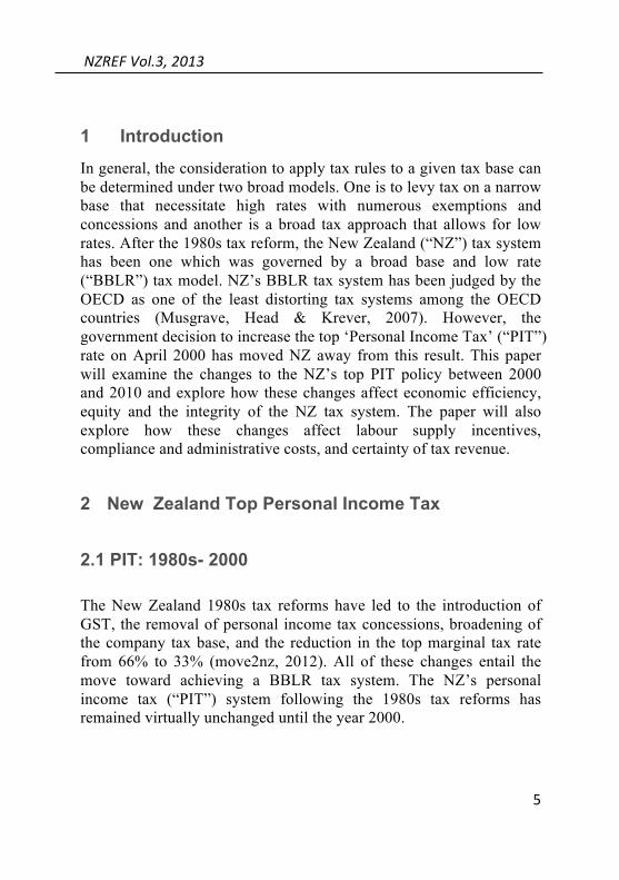
Improvement in equity, in effect, comes at the cost of efficiency when additional government spending is financed through higher top marginal tax rates. This is because the subsequent resources transferred from the private economy to the public sector under such policy not only reduce top-earners’ income through the direct burden of taxation, but also may distort welfare as these individuals base their behaviour (e.g. investment decisions) on tax considerations (Carroll & Prante, 2013; New Zealand Treasury, 2009). This distortionary cost to welfare in addition to the direct cost of taxation is called the excess burden of taxation (New Zealand Treasury, 2009). Excess burden of taxation reflects the fact that taxpayers rearrange their affairs in ways that are different and less desirable following the rate changes (New Zealand Treasury, 2009). The increase of top PIT rate from 33% (m) to 39% (m’) would cause excess burden to increase from the area BAC to BA’C’ as illustrated in Figure.

The change in the size of excess burden arising from the change in tax policy is referred to as the marginal excess burden of tax (“MEB”) (Hines, 2007). The MEB per dollar of extra revenue, in turn, provides a measure of the ‘Marginal Welfare Cost’ (“MWC”) of the tax change (New Zealand Treasury, 2009). Under the assumption that the marginal tax rate is below the revenue-maximizing rate, one can use the following equation to quantitatively estimate the MWC.

 NZREF  Vol.3,  2013    

 

7  

!"#$%&"'  !"#$%&"  !"#$ =!. !"# . !"#  !"#$

1 − !"#  !"#$ − !. !"# . !"#  !"#$  

(New Zealand Treasury, 2009)

This equation suggests that MWC per dollar of additional tax revenue not only increases as tax rate increased; it also increases when elasticity of taxable income (“ETI”) and the ratio of the average income above the tax threshold to the threshold income level (“!”) increased. Numerous studies have shown that the ETI for top income-earners are in excess of 0.5 and can be as high as 1.1 (Claus, Creedy & Teng, 2012). A study by Alastair Thomas (2007) on ETI and the deadweight cost of taxation in New Zealand has provided a preferred estimate for ETI of 0.52 (cited in Claus, Creedy & Teng, 2012). Given

Figure 1: Effect of Marginal Tax Rate increase on Welfare

S*  (compensated  

Labour  supply)  

W  

Wage  Rate  

(1-­‐m)W  

(1-­‐m’)W  

B  C’  

A  

A’  

L1  L2  L3   Labour  

C  

(Browning, 1987, p. 12)

 NZREF  Vol.3,  2013    

8  

an ETI of 0.52 and the ! values estimated by the New Zealand Treasury, one can compute the MWC corresponding to changes in top PIT policy between 2000 and 2010 as follow.

Table 1: MWC (Per $ of additional tax revenue) for New Zealand

Year

Tax rate = 33%

Alternative tax rate

α= average top PI/threshold

Thomas (2007) preferred ETI = 0.52 then MWC:

1999 33% 2.27 1.39

2001(Top PIT increase) 39% 2.54 5.43

2008 (Thresholds increase) 39% 2.52 5.17

2010 (Top PIT decrease, GST increase) 33% 2.54 1.86

(Claus, Creedy & Teng, 2012; Creedy & Gemmell, 2012)

From Figure 2, one can infer that the MWC per extra dollar of revenue raised with ETI of 0.52 is well in excess of a dollar (Claus, Creedy & Teng, 2012) and that the introduction of the 39% top PIT rate has caused MWC to increase substantially, from $1.39 to $5.42. This substantial increase in MWC indicates that increasing tax revenue by raising top PIT rate is very costly in terms of efficiency. In fact, Thomas (2007) has also shown in his study that if ETI is higher, then a 39% top PIT rate can result in a MWC to being as high as $8 per extra dollar of revenue raised (New Zealand Treasury, 2009). The New Zealand Treasury’s study on ETI in New Zealand has further shown that the MWC increases more than proportionately as ETI

 NZREF  Vol.3,  2013    

 

9  

increases and that marginal tax rates tend to exceed the revenue-maximizing tax rate when ETI is greater than 0.7 (Claus, Creedy & Teng, 2012). Therefore, due to the high ETI of the high-income earners, imposing a higher top PIT rate would likely to cause a substantial increase in MWC.

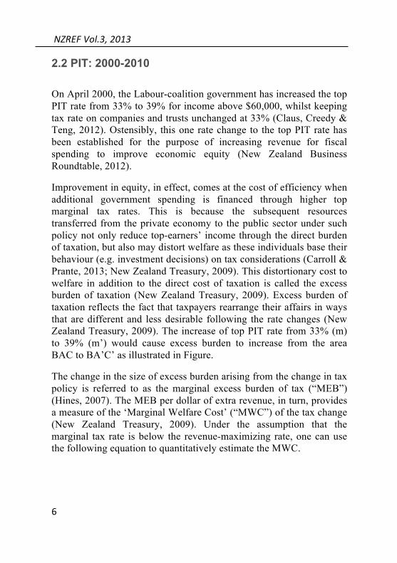
International evidences have shown that for top-earners, taxes have no effect on their labour supply decision at the extensive margin and have very little impact at the intensive margin given the low labour supply elasticity of this income group, particularly that of ‘prime age males’, those between 20-44, (Claus, Creedy & Teng, 2012; Saez, Slemrod & Giertz, 2012). This suggests that the labour supply incentive effect with respect to the reduction in disposable income would be small (Creedy, 2009). Figure 3 provides a graphical illustration of this.

0  

2  

4  

6  

1999   2000-­‐2001   2008   2010  

Figure  2:  MWC  es.mates  with  EIT  =  0.52  

EIT  =  0.52  

 NZREF  Vol.3,  2013    

10  

However, the top PIT hike of 39% do affect top-earners’ taxable incomes, such that they would respond by reorganizing their affairs to take advantage of the way different sources of income are taxed to reduce their tax liability (Meghir & Phillips, 2009). The misalignment between top PIT rate (39%) and the tax rate on companies and trusts (33%) have provided a means for such reorganization (Zhang, 2007). Consequently, trusts and companies have been used to shelter income that would otherwise be taxable at 39%. Hence, the misalignment of these rates has incentivized the use of companies and trusts as tax sheltering devices for lawful tax avoidance (Law Commission, 2010; IRD, 2011). This form of tax avoidance is defined as “tax arbitrage across income streams facing different tax treatment” by Joseph Stiglitz in his general theory of tax avoidance (Stiglitz, 1986; Slemrod & Yitzhaki, 2002).

According to Stiglitz (1986), in an imperfect market economy, tax avoidance would reduce tax liability and thereby the excess burden of tax. However, tax avoidances generally achieved using resources, such as accountants and lawyers, who have alternative productive use. Additionally, tax avoidance does undermine the integrity of the tax

S  

Income  

 Leisure    

Hours    

 

 (Brown & Jackson, 1990)

Figure 3: Income-Leisure Model

 NZREF  Vol.3,  2013    

 

11  

system, whereby forcing the government to devote resources toward counteracting it in order to secure necessary revenue and to ensure all source of taxpayers’ taxable incomes are correctly deducted (IRD, 2011). Consequently, this has led to the establishment of complex anti-avoidance rules in New Zealand to prevent tax avoidance for certain types of personal income earned through companies (Saez, Slemrod & Giertz, 2009). Clearly, from societal perspective, these inefficient uses of resources serve as an argument that tax avoidance would lead to greater economic distortion rather than lessening it.

Furthermore, the introduction of the complex anti-avoidance rules has added legal and economic complexity to the tax system, and thus fueling the growth in compliance and administrative costs. The reallocation of income from one source to another to reduce tax liability has also created uncertainty in government revenue, whereby the top PIT hike of 39% instead of increasing revenue as expected, has actually led to lower tax revenue. Between 2001 and 2008, the top percentile of income earners has only contributed on average 9.3% of personal income tax revenue, which is lower than the 10.2% average figure between 1994 and 2000 (Claus, Creedy & Teng, 2012).

Moreover, the arbitrage opportunities for tax avoidance has caused the objectives of increasing top PIT as a means of improving equity to become the mechanism that worsens it instead. Vertical inequity results because the benefit of the availability of tax arbitrage opportunities and thus the access to companies and trusts as a means of reducing tax bills only goes to those at the top of the income distribution. Hence, those earning more can rearrange their affairs to pay less tax. This option is not available to everyone. It is also horizontally inequitable when income growth between 2001 and 2008, under fixed thresholds in nominal terms, has pushed a large number of taxpayers into the high tax bracket, resulting in Fiscal Drag (IRD, 2011). Hence, those at the same situation could not be treated equally because not everyone in the top PIT bracket are high income earners that own a company or have access to trusts for such advantage.

 NZREF  Vol.3,  2013    

12  

Increasingly, ‘Fiscal Drag’ has become the center of political debate as incomes’ growth push more and more people into the next tax bracket. Political pressure from headline such as “Bracket racket has cost taxpayers $10b –ACT” (NZPA, 2008), and accusation that the “government has pocketed close to an extra $2 billion in fiscal drag since their eight years in office” (O’Sullivan, 2008), have forced the government to increase all PIT thresholds. On October 2008, the top PIT threshold has increased to $70,000 (New Zealand Treasury, 2008). This has led to a slight decrease in the MWC, and thus the excess burden of tax in 2008 through its effect on reducing the α value for top income earners from 2.54 to 2.52, as illustrated in Table 1 and Figure 2 above.

Increasing tax thresholds with no change to marginal tax rate will have a pure income effect for individuals earning above that threshold (Meghir & Phillips, 2009). This is because the potential tax savings estimated using “tax calculator” remain constant at $2070 for those earning $70,000 and above (NZIER, 2007), and thus there is no incremental benefit to induce a substitution toward more hours of work. However, for those earning between $60,000 and $70,000 dropping out from the top tax bracket, the proportion of tax savings increases as their taxable income increases (NZIER, 2007), thereby providing an incentive to increase hours of work.

The increase of the PIT thresholds to counter the effect of Fiscal Drag has made an improvement to both horizontal and vertical equity by alleviating the inflationary effect on individuals’ income that push them into the next tax bracket. However, with no changes to the top PIT rates, the misalignment between top PIT rate and that of trusts and companies still persisted, and thus the problems caused by arbitrage activities of lawful tax avoidance remained. The inefficiency, unfairness, cost ineffectiveness, and inferior revenue resulting from tax avoidance activities incentivized by the misalignment of tax rates as outlined above would still prevail.

2.3 PIT: 2010-2012

 NZREF  Vol.3,  2013    

 

13  

The growing concerns over tax avoidance, particularly through trusts as income shelters. After an IRD’s report found that “half of NZ’s super-rich dodge tax” (Levy, 2012), the new National-led government took measure to realign the top PIT rate with the tax rate for trusts at 33% in 2010 (Law Commission, 2010). Additionally, international competitive pressure and the need to boost the NZ’s economy via increase investments, following the 2008 financial crisis, have led the government to reduce the company tax rate to 30%. The realignment of tax rates between top PIT and trusts combined with the already established anti-tax avoidance rules, in turn, reduced the benefits of tax savings from income shifting activities. According to Stiglitz’s principles of tax avoidance, it follows that the removal of tax savings from arbitrage opportunities between different income streams would remove the incentive for tax avoidance (Stiglitz, 1986). Hence, the costs to efficiency, equity, and integrity of the tax system deriving from tax avoidance would be eliminated.

Under the 2010 tax policy, MWC estimates to decrease to $1.86 per extra dollar of revenue raise, whilst holding ETI at 0.52, as illustrated in Figure 2. Hence, the reduction of the marginal top PIT rate would lead to a further reduction in inefficiency. Such policy, however, does come at a cost. The back of envelope fiscal costs of the 2010 PIT policy estimates to be $5.5 billion (NZIER, 2007). In order to offset such cost to the government budget, the government has also increased the rate of GST from 12.5% to 15% (IRD, 2010). The combination of lowering PIT rate and increasing broad base consumption tax, such as GST, is a shift back to the 1980s BBLR tax system.

The BBLR approach would reduce the economic harm of raising revenue by lowering the cost of tax on any particular source and minimizing the behavioral changes caused by taxation (VUW Tax Working Group, 2010). This occurs because low rate would reduce the incentives and opportunities for tax avoidance (VUW Tax Working Group, 2010). The reduction in tax avoidance combined with

 NZREF  Vol.3,  2013    

14  

the administrative simplicity of GST with very few exemptions would lead to the reduction in compliance and administrative costs of taxation.

There is also a noticeable improvement to the government collection of tax revenue, despite the modest tax rates under the BBLR approach. NZ has collected greater tax revenue from its major tax bases, valued at $51.6 billion, for the 2010/11 compared to the $29.92 billion in 2001 (IRD, 2011a; IRD, 2011b; New Zealand Treasury 2012). This is because when GST is ran in parallel with PIT, the risk of revenue losses would be reduced as revenue base is spread across a number of independently enforced sources (VUW Tax Working Group, 2010). Consequently, this has induced greater certainty to tax revenue collection. Hence, the move toward a BBLR under the 2010 tax policy has led to the improvement in efficiency and integrity of the tax system. However, these improvements to efficiency do entail a cost to vertical equity given that low-income earners do spend a higher proportion of their total income on consumption than high-income earners. Hence, those who earned more are not necessarily taxed more. This cost, somewhat, has been offset by the improvement to horizontal equity with the introduction of the inflation-adjusted tax rate thresholds to fully account for inflationary pressure at the same time.

3 Conclusion Overall, the government decision to increase the top ‘Personal Income Tax’ (“PIT”) rate on April 2000 has had very little effect on labour supply incentives at the intensive margin due to the low labour supply elasticity of this income group. However, higher top PIT rate and its misalignment with the tax rate on trusts and companies have incentivized top earners to engage in lawful tax avoidance in order to reduce their tax liabilities. Consequently, tax avoidance has led to the deterioration of economic efficiency and equity. Importantly, it has undermined the integrity of the NZ tax system, whereby inducing greater compliance and administrative costs and creating uncertainty in government revenue. Although the introduction of higher PIT tax thresholds in 2008 has made an improvement to equity by eliminating

 NZREF  Vol.3,  2013    

 

15  

the inflationary effect on income, it does not solve the problem of tax avoidance when the misalignment of rates remains. It is only when potential tax savings from arbitrage opportunities between different income streams are removed that the inefficiency, unfairness, cost ineffectiveness, and inferior revenue resulting from tax avoidance can be eliminated. The shift towards the BBLR approach in the 2010 tax policy is a step toward achieving these objectives.

References Brown, C.V. & Jackson, P.M. (1990). Public Sector Economics. Oxford: Blackwell Publishers Ltd. Browning, E.K. (1987). On the Marginal Welfare Cost of Taxation. The American Economic Review, 77 (1). Retrieved from http://lsfiwi.wiso.uni-potsdam.de/posa/2006/dozenten/Truong/browning.pdf. Carroll, R., & Prante, G. (2013). Long-run macroeconomic impact of increasing tax rates on high-income taxpayers in 2013. Retrieved from http://majorityleader.gov/uploadedfiles/Ernst_And_Young_Study_July_2012.pdf Claus, I., Creedy, J., & Teng, J. (2012). The Elasticity of Taxable Income in New Zealand: New Zealand Treasury Working Paper 12/03. Retrieved from http://www.treasury.govt.nz/publications/research-policy/wp/2012/12-03/twp12-03.pdf.

 NZREF  Vol.3,  2013    

16  

Creedy, J. (2009). The Personal Income Tax Structure: Theory and Policy. Retrieved from http://www.victoria.ac.nz/sacl/cagtr/pdf/creedy.pdf. Creedy, J. & Gemmell, R. (2012). The Elasticity of Taxable Income and the ‘Laffer Effect’. Retrieved from http://www.business.otago.ac.nz/econ/seminars/Abstracts/2012/Gemmell30Mar.pdf. Hines, J.R. (2007). Excess Burden of Taxation. Retrieved from http://www.bus.umich.edu/otpr/WP2007-1.pdf. IRD. (2010). GST rate increase. Retrieved from http://taxpolicy.ird.govt.nz/publications/2010-sr-budget2010-special-report/gst-rate-increase. IRD. (2011). Policy Challenges. Retrieved from http://taxpolicy.ird.govt.nz/publications/2011-other-bim/3-policy-challenges. IRD. (2011a). The New Zealand tax system and how it compares internationally. Retrieved from http://taxpolicy.ird.govt.nz/publications/2011-other-bim/2-new-zealand-tax-system-and-how-it-compares-internationally. IRD. (2011b). Revenue collected, 2001 to 2010. Retrieved from http://www.ird.govt.nz/aboutir/external-stats/revenue-refunds/tax-revenue/revenue-refunds-tax-revenue.html. Law Commission. (2010). Some Issues with the use of Trusts in New Zealand: Review of the Law of Trusts Second Issues Paper. Retrieved

 NZREF  Vol.3,  2013    

 

17  

from http://www.lawcom.govt.nz/sites/default/files/publications/2010/12/trusts_second_issues_paper_72.pdf. Levy, D. (2012). Half NZ’s super-rich dodge tax. Retrieved from http://www.stuff.co.nz/business/money/7549236/Half-NZs-super-rich-dodge-tax. Meghir, C. & Phillips, D. (2009). Labour Supply and Taxes. Retrieved from http://elsa.berkeley.edu/~saez/course/Hausman_Handbook.pdf. Musgrave, R.A., Head, J.G., & Krever, R.E. (2007). Tax Reform in the 21st Century: A Volume in Memory of Richard Musgrave. Netherland, Kluwer Law International. move2nz. (2012). Taxation in New Zealand. Retrieved from http://www.move2nz.com/nz/nz_taxes.aspx. New Zealand Business Roundtable. (2012). Is ‘Tax the Rich’ Good Policy? Retrieved from http://www.nzbr.org.nz/site/nzbr/files/Is'Tax%20the%20Rich'%20Good%20Policy.pdf. New Zealand Treasury. (2008). What is the new personal income tax scale? Retrieved from http://www.treasury.govt.nz/budget/2008/taxpayers/01.htm. New Zealand Treasury. (2009). Estimating the Distortionary

 NZREF  Vol.3,  2013    

18  

Costs of Income Taxation in New Zealand. Retrieved from http://www.victoria.ac.nz/sacl/cagtr/twg/publications/5-estimating-the-distortionary-costs-of-income-taxation-in-newzealand-treasury.pdf. New Zealand Treasury. (2012). Revenue. Retrieved from http://www.treasury.govt.nz/government/revenue. NZIER. (2007). Final Tax Cut Calculator –B.xls. Retrieved from https://blackboard.vuw.ac.nz/webapps/portal/frameset.jsp?tab_tab_group_id=_2_1&url=%2Fwebapps%2Fblackboard%2Fexecute%2Flauncher%3Ftype%3DCourse%26id%3D_58376_1%26url%3D. NZPA. (2008). ‘Bracket racket’ has cost taxpayers $10b – ACT. Retrieved from http://www.stuff.co.nz/national/politics/420046/Bracket-racket-has-cost-taxpayers-10b-ACT. O’Sullivan, F. (2008). Fran O’Sullivan: Fiscal drag a real downer. Retrieved from http://www.nzherald.co.nz/business/news/article.cfm?c_id=3&objectid=10512313 Saez, E., Slemrod, J., & Giertz, S.H. (2009). The Elasticity of Taxable Income with Respect to Marginal Tax Rates: A critical Review. Retrieved from http://elsa.berkeley.edu/~saez/saez-slemrod-giertzJEL09elasticity.pdf. Saez, E., Slemrod, J., & Giertz, S.H. (2012). The Elasticity of Taxable Income with Respect to Marginal Tax Rates: A critical Review.

 NZREF  Vol.3,  2013    

 

19  

Journal of Economic Literature, 50 (1). Retrieved from http://elsa.berkeley.edu/~saez/saez-slemrod-giertzJEL12.pdf. Slemrod, J. & Yitzhaki, S. (2002). Tax Avoidance, Evasion, and Administration. Retrieved from http://elsa.berkeley.edu/~saez/course/Slemrod,Yitzhaki%20PE%20Handbook%20chapter.pdf. Stiglitz, J.E. (1986). The General Theory of Tax Avoidance. Retrieved from www.nber.org/papers/w1868. VUW Tax Working Group. (2010). A Tax System for New Zealand’s Future. Retrieved from http://www.victoria.ac.nz/sacl/cagtr/pdf/tax-report-website.pdf. Zhang, L. (2007). Tax Avoidance: Causes and Solutions. Retrieved from http://aut.researchgateway.ac.nz/bitstream/handle/10292/13/ZhangLBecky.pdf?sequence=1.

 NZREF  Vol.3,  2013    

20  

An Overview of

Development State in Thailand: Formation and Implementation of State

Capacity Long VO2

Abstract

State development capitalism, also referred to as developmental state, is an economic model characterized by a government taking responsibility to deliver steady growth via intervention and extensive regulation. Originated from East Asia, this model necessitates the role of the states in mobilizing social resources in order to support cohesive industrialization policies. This article examines one of the successful state-led developments, namely Thailand. By critically reviewing the historical records of the Thai state’s development up to the late 1990s, it can be observed that this state is distinctive in the sense that whilst it secures sufficient politico-cultural leadership, it lacks the capacity to implement coherence to its coercive policies.

                                                                                                                         2  I  thank  Louise  Lamontagne  for  her  inspiring  encouragement  during  the  course  of  ECON421.    I  am  also  grateful  to  two  reviewers  from  the  NZREF  Editorial  Board  for  helpful  comments.      All  remaining  errors  are  my  own.  E-­‐mail:  long.vo@vuw.ac.nz.    

 NZREF  Vol.3,  2013    

 

21  

1 Introduction

Developmental state, or hard state, is a term originally used by political economists to refer to the phenomenon of state-led macroeconomic planning in East Asia in the late twentieth century. In this model of capitalism (sometimes referred to as state develop- ment capitalism), the government has more independent, or autonomous, political power, as well as more control over the economy. A development state is characterized by having strong intervention, as well as extensive regulation and planning.

The first person to conceptualize the developmental state was Johnson (1982). He wrote in his book “MITI and the Japanese Miracle”: “In states that were late to industrialize, the state itself led the industrialization drive, that is, it took on developmental functions. These two differing orientations toward private economic activities, the regulatory orientation and the developmental orientation, produced two different kinds of business-government relationships” (p.19).

A notable feature of a typical regulatory state is the use of regulatory agencies empowered to enforce a variety of standards to protect the public against market failures and abuses of market power. A regulatory state also complements the market in providing public goods. In contrast, a developmental state intervenes more directly to the economy through a variety of means to promote the growth of new industries and to reduce the dislocations caused by shifts in investment and profits from old to new industries. In other words, developmental states can pursue industrial policies, while regulatory states generally cannot.

Ever since Johnson (1982) proposed the concept, academics worldwide had come to a general agreement regarding the fundamentals of the developmental state. The idea of “a centralised state interacting with the private sector from a position of pre-

 NZREF  Vol.3,  2013    

22  

eminence so as to secure development objectives” (Wade, 1990) is now generally known as the developmental state theory (See also (Johnson, 1982; White & Gray, 1988)). These states are driven by an urgent need to promote economic growth and to industrialize (Leftwich, 1995) to catch up with the West and the industrialized neighbours. Specifically, what is meant by a developmental state, is a government with sufficient organization and power to achieve its development goals (Woo, 1999). Similarly, (Doner, Ritchie, & Slater, 2005) argued that in order to facilitate national economic transformation a developmental state must have “expert and coherent bureaucratic agencies collaborate with organized private sectors”.

Thailand is considered to fall between the U.S. model where government has relatively little involvement in economic policy, and Japan which has governed with a very heavy hand (Kulick & Wilson, 1996; Muscat, 1994). One example of Thai development policies was its import substitution. Only a hard state is influential enough to enforce high import tariffs to protect infant domestic industries, especially when such trade-barrier policy undermines the benefits of not only large multinational firms but also of their own rich citizens.

In this essay I will focus on discussing most notable features of Thailand’s develop- mental state. In particular, I intend to examine Thai government’s ability to demonstrate rational economic guidance and efficient organization, and most importantly its power to back up economic policies. In addition, it is interesting to review academic opinions regarding the degree to which Thai state was able to resist external pressure from international forces for their short-term gain and overcome internal resistance from strong interest groups. Given the limited scope of this essay, the main focus is to provide a lit- erature review of Thai government’s characteristics up to the late 1990s when the world witnessed the Asian financial crisis. Specifically, following the definition of a “hard state”, I seek answers for two basic questions: Where did the Thai state’s power comes from? And how did it utilize this power to achieve success on par with other “Asian miracles”? These examinations are to provide useful

 NZREF  Vol.3,  2013    

 

23  

implications for Thailand during the post-crisis period and future development.

The rest of the paper will have the following structure: section 1 discusses the formation of Thai developmental state, section 2 presents the process of state power consolidation, section 3 looks at the influence of state economic policies and section 4 concludes.

2 Formation of Thai Development State

2.1 PIT: Early Foundations In order to understand the role of Thailand’s developmental state, I believe it is essential to examine its origin, which could be traced back to the birth of the People’s Party in the Constitutional Revolution in 1932. Going further back, in a recent report, Ishikawa (2008) provided a relative comprehensive review of Thai democratic reform since the Sakdine system (which began in the 14th Century). Mainly based on his report, this section discusses Thailand’s political instability, characterized first by a forced change from absolute monarchy to constitutional democracy in 1932.

In essence, Thai political philosophy is rooted from the concept of “patrimonial- ism” (first proposed by (Weber, Roth, & Wittich, 1978)) which describes the relation- ship among three key actors: ruler, administrative officers and subjects. According to (Ishikawa, 2008:5), legitimacy is one crucial condition to patrimonial system existence, “ by tradition, legitimacy is derived from trust in the sanctity of an order that has existed since time immemorial. Once this trust was weakened or lost, patrimonialism faces a crisis of legitimacy”. This author also raised the intriguing point that the monarchic patrimonialism in Thailand was established based on the “good deeds performed in former Buddhism incarnations”, instead of

 NZREF  Vol.3,  2013    

24  

being influenced by the Confucian idealism as seen in China (p.31). Indeed, until the early 20th century, Thai kingdoms were under ab- solute rule of kings. However, this system was replaced by administrative reforms during the Chakri (Bangkok) Dynasty. The reform was completed by a democratic revolution in 1932 led by conservative military and western-influenced civil officers, which aimed at the monarchy and Chinese-origin groups in private sector.

It resulted in the formation of the People’s Party and marking the beginning of a constitutional monarchy. However, we should be clear in our understand of the nature of this Thai-style democracy, as it is at the core of the development state evolution. In a very intuitive article, Schmidt (1993) saw the 1932 Revolution, and many similar subsequent coups, not as being a democratic movement, but as a “reflection of the shift from absolutism to Thai-style democracy”. On the surface, a Western-ideological parliamentary system was adopted. In truth, what happened is only a structural shift within the ruling elite. Furthermore, by maintaining the authority of the monarchy though limited, the new government preserved a symbol that could reduce the effort in “establishing their legitimacy in the minds of that portion of the population that is politically conscious”(Thinapan, 1972:55). Handley (2006) even went so far as portraying the current Thai King Rama IX as “an anti-democratic monarch who, together with allies in big business and the murderous, corrupt Thai military, has protected a centuries-old, barely modified feudal dynasty”.

Suehiro (1985) argued that the most important outcome of the 1932 coup was the expansion of profit making activities, characterized by the promotion of an industrial sector “with the goal of establishing a seft-sufficient economic system”. The People’s Party, however powerful, did not have a fiscal foundation. According to Fujiwara (1994), early established state-owned enterprises were based on powerful party members who only fight for their factions’ interests. Schmidt (1993) supplemented this point by stating that Thai industrial sector was first created only after the 1958 coup, which will be described below.

 NZREF  Vol.3,  2013    

 

25  

2.2 Thai – style Democracy Ten years since the Revolution, in the late 1950s and early 1960s, Thai-style democracy was completely implanted into political system by Prime Minister Sarit. He banished his predecessor, Phibun Songkhram, who tried to adopted Western-style, parliamentary democracy in Thailand. The Sarit system formation is described as a “decisive political factor in the formation of post-World War II Thai society” by Suehiro (1993). In addition, several researchers documented that expulsion of army leaders controlling bureaucrat enterprises was essential to the solidification of the political foundation of the Sarit system. Ishikawa (2008) listed three core concepts as the ideology supporting this regime: (1) the central philosophy was the ancient principles of Nation, Religion and King and this resulted in a reinstatement of the authority of the King; (2) the goal of establishing a developmentalist regime similar to Indonesia and the Philippines (I believe this concept is analogous to our modern note of Developmental state); and (3) “Politics by father and King” or “Thai-style democracy” as oppose to its Western-style counterpart. These concepts were propagated and legitimized to help settled the party infighting and setting the patterns of politics and economics prevalent in post-war Thailand. Throughout the relevant literature, I found a relatively strong agreement upon the point that there was a dramatic change in Thailand’s political philosophy during the Sarit reform. Analogous to the concept of Thai-style democracy, Thak (2007) also described a “Thaification” process as the replacement of the traditional political system inherited from 1932 by modernization on the basis of Thai values and culture. By and large, it could be concluded that the early seeds of Thailand developmental state were sowed in this period.

The foregoing generally described the context of the early foundations of Thailand’s developmental state. From this time point onward Thai politics became an arena for competing factions among both old and new agencies. Then the centre question arises: Within such highly volatile political background, what measures could the

 NZREF  Vol.3,  2013    

26  

state take to fulfil its promise to deliver steady economic growth? To my knowledge, there is no simple answer, but one possible explanation is the existence of negotiation among these factions that helped restore temporary stable periods of semi-democracy.

3 The Rise of Thai Developmentalism

3.1 Distinctive Features of the State

Given the above insights, our concern now is what constitutes Thai-style democracy? And how does it help consolidate the developmental state? To answer these questions, again, we turn to history. In the wake of post-Sarit era, the Thai political situation did have two important and distinctive features: firstly, successive political parties had taken power alternately for short periods of time. This is very different from contemporary long-term running parties in contemporary adjacent South East Asian nations such as Indonesia, Malaysia or Singapore, a phenomenon described as “government party” by Fujiwara (1994). This author also pointed out that from the perspective of the prevailing politics by father and King, the adoption of the government party system and its characteristically long-term administrations are likely to “pose unacceptable threats”. Interestingly, Schmidt (1993) and Dixon (1991) agreed upon the view that only in Thailand governments have been short-lived and investors “seem to be accepting that even with changes of government brought about by coup d’etat, there is little threat to investment” (Dixon, 1991:14). Secondly, the post-Sarit period witnessed the rise of urban middle class and pro-democracy movements. The enhancement of primary and higher educations as a part of economic development in this era had led to a rapid increase in the number of students and a remarkable expansion of the middle

 NZREF  Vol.3,  2013    

 

27  

class. As a result, in the early 1990s, these groups repeatedly clashed with authorities in demanding a democratic system and criticized the military corruption.

The afore mentioned events, together with the notion that the world-wide shift to democratic regimes from authoritarian ones became a common scenario of politics during the last decades, had attracted the attention of Schmidt (1993). One major argument of his paper is that the transition to democracy in Thailand is determined by state control rather than by forces of civil society or the business sector. Rather, it were Thai “specific political culture” and “loosely structured social system” that contributed to the independence with which Thailand was able to resist the imposition and transfer of institutions from the West happened in many developing countries (Diamond, Linz, & Lipset, 1900). In his study in 1971, Jacobs (1971) made a comparison between Japan and Thailand by stating that these two countries were able to prevent direct colonization thanks to their “hard state”.

Different from the United States, in these countries the system of ministries were created not as civil servants, nor to provide regulation of private concerns, or to create jobs for party supporters, but rather “to guide forced development”. As Schmidt (1993) stated it, “the hegemonic role of the military within the state contributed to the creation and expansion of some successfully coherent developmental policies”. Arguably, developmental strategies were adopted not for the sake of development itself, but served as a mean to promote administrative of society, thus explaining why Western con- stitutional democracy was considered inappropriate in Thai system. This fundamental point is similar to that made in one of Doner et al. (2005)’s most intuitive paper, that rather than arising from their

 NZREF  Vol.3,  2013    

28  

love for nation, developmental states were facilitated by of political leaders’ recognition that - under pressure of systemic vulnerability (such as democratic demands in Thailand’s case) - only a coherent bureaucracy could produce necessary resource to maintain the fragile coalitions and thus secure state sustainability.

3.2 Internal Paradox and Democratization

Since becoming a semi constitutional democratic monarchy in 1932, for most of the time Thailand has been ruled by military governments. Given the goal of the new development policy and the role of the state in Thailand, we could expect dissatisfaction from the population. Indeed, civilian protests and insurgencies against the rule of military leaders happened from time to time since 1932 ended up brutally suppressed, most no- table are the 1976 massacre and the 1992 Black May uprising. During these periods, the ruling power fluctuated between unstable civilian governments and interludes of military takeover. To maintain the power of the military wing and political stability, intensive repression of population was necessitated (Somsak, 1987). However, there is one civil interest group that benefited from this settlement - the Sino-Thai business class which had become the dominant force in economic field.

Douglas (1984) documented a strong but unstable alliance between the Chinese merchants and Thai military, which resulted in a “paradoxical” situation where government officials sat on the boards of private enterprises while Sino businessmen served as managers of state enterprises “originally established to keep some economic activities out of their hands” (Brewster, 1974). According to Schmidt (1993), the military acted as a proxy to a Thai-origin business sector, and a counter factor to the Chinese. Despite the complex and unorthodox pattern of the Thai state, I believe it is adequate to claim that the alliance of these two primary rival forces was the under- lying driving factor of Thai developmentalist economic course post-1932. Doner et al. (2005) elaborated this point by examining

 NZREF  Vol.3,  2013    

 

29  

and comparing several institutional features of the developmental states in the ASEAN-4 (Malaysia, the Philippines, Indonesia and Thailand). He found an asymmetry in the bureaucratic structure in which clientelism and sector factionalism signifies the public-private linkages.

It is worth examining in more detail the most notable democratic period in Thai- land - from October 1973 to October 1976 (a period aptly named Thai Spring) - when the legitimized institutions of the state were temporarily overthrown by a new civilian government. As mentioned above, Thai’s state capacity is a result of a combination of coercive and in-corporative measures which allowed for manipulation of population. However, this settlement was not enough to repress public opposition when the state planned to extract resources from agriculture for industrial development. Evenson (1983) exemplified the infamous rice premium enforced toward facilitating import-substitution and subsequent export-oriented strategies, which resulted in rice shortage and rice export prohibition in 1973.

State capacity to implement this policy was effective when simultaneously promoting stability in urban areas and poverty in rural sector. Another factor contributed to the growing democratic demand is social unrest built up after two decades of martial law and dictatorial rule. Robust student movements, fuelled by the unjust seen in this period of “state squeezing of farmers”, sought to replace the Thai-style democracy ideologies and seek new values in changes. The media received more freedom to criticize politicians and governments, while revolutionary and socialist positions became more apparent. However, similar to past recurring uprisings, this movement’s influence was very short-lived, and it did little in changing the state apparatus. The reforms were reversed after a staged coup and subsequent massacre in 1976 by the armed forces. The military dominated bureaucracy remained intact and continually involved

 NZREF  Vol.3,  2013    

30  

in new strategies of state interventionism, both socially and economically.

3.3 Foreign Relations

Throughout its history, Thai state heavily relied on external power to maintain the country’s independence. Examples range from patron-client relationships between Thailand and British to military agreements with Japan and the U.S (Lau & Suryadinata, 1988). In this section, I provide a brief discussion of the ability of Thai state to adjust and maintain their role while interacting with these powers. From the 1960s Thailand had been fitting its role in American long-term design as a buffer preventing the spread of Asian communism. It can be observed that the leading role of the military in Thailand was by no mean autonomous, rather, it was facilitated mostly via American aid.

Extending this point, Muscat (1990) pointed out that the capacities of Thai state agencies were designed as a part of American Cold War foreign policies. In addition to the U.S. government, large international organizations also exerted significant influence on the regime-form, the state and the development policies of Thailand through aid, loans and policy recommendations (Ingram, 1971). As a result of this, the bulk of FDI to Thailand was directed toward an important strategy shift in the late 1970s: from predominantly import substitution to export oriented industrialization. Moreover, in the early 1980s, by the Structural Adjustment Loans, the IMF and the World Bank urged Thai state to restructure its economy and stop subsidizing public utilities and old prices. As Hewison (1985) concluded in his article: “the supply of large loans and credits by international agencies and private transnational banks gives them a considerable stake in the direction of (Thailand) national development and provides international finance capital with a strong stimulus to influence development policies”(p.60).

 NZREF  Vol.3,  2013    

 

31  

Since the late 1980s and the beginning of 1990s, Japanese economic impact and subsequent political and cultural influence have grown tremendously not only in Thailand but in East Asia (Nester, 1990a, 1990b). After American’s defeat in Vietnam, the withdrawal of the U.S. troop from Thai territory left an exhausted Thai domestic market. This is when the Japanese moved in and solved the problem of outlets for Thai products. During this period, Thailand called for significant economic aid and investment from Tokyo as Japan became the leading economy in the region.

One important evidence of Thailand’s technical dependency is the lack of a radical land reform. As a matter of fact, international aid depends on orthodox prerequisite of privatization, while neglecting intervention in rural economy. Different from Japanese development process, in Thailand there was virtually no major changes in land owner- ship structure, and farmers without lands were not qualified for bank loans necessary for rural development (Wonghanchao, 1988).

As a result of international influence, a triangular economic relationship was created between Thailand, Japan and the U.S in which Thailand provided raw material in ex- change for technology and capital. By mid 1970s, Japan replaced the U.S. as the region’s most important trader and investor. The vast inflows of foreign direct investment to Thailand not only reshaped its development strategies but also created heavy dependency on external technological and financial resources. Evidence of this trend are the dominance of foreign financed firms where Japanese shareholders maintain major control (Soon, 1990). Overall, although Thailand’s integration into the capitalist world has resulted in a limited and externally determined capacity, it created crucial conditions to legitimize the authoritarian state.

4 Role of the State in the Economic Growth

 NZREF  Vol.3,  2013    

32  

Although playing a major role in domestic development, when compared to the success of implemented coherent and rational industrial policies in Japan, Taiwan or Korea, Thai state has not had the same capacity to rationalize its economic policies and secure the expected objectives of its development plans (Ikemoto, Wonghanchao, & Ajia, 1988). In other words, it did not fit very well to Doner et al. (2005)’s definition of the developmental “hard state” in terms of effective and coherent bureaucracy. Thai state’s independence from society may have given it the power to implement development policies, but it also lost the ability to mobilize public support.

At the end of the Second World War, Thailand was one of the world’s poorest countries. In sharp contrast, between 1955 and 1988, per capita economic growth in Thailand averaged 3.9 per cent per annum (Richter, 2006:8). High economic growth was accompa- nied by a rapid decline in the incidence of poverty, mild but rising income inequality, and substantial exports of both manufactures and primary commodities, including processed agricultural commodities. Though the changes in the Thai economy in this period was remarkable, positive results could only be observed after the decisive shift to an export- oriented strategy since 1985. However, it is questionable in which way these changes can be attributed to the development strategies. With respect to this, (Dixon, 1991:206) offered a timing point of view, that the policies “facilitated changes made possible by the development of the international economy”. Schmidt (1993) alleviated this point by describing the military dominated state bureaucracy as an intermediary between interna- tional and Sino-Thai economic interests. In general, promotion of industries to transform the Thai traditional society into a modern industrial economy was - and still is - the fundamentals underlying the state’s reform policy over the past three decades. To reach this ultimate end, the opening of economy and society to foreign capital integration is crucial. Therefore state planning in Thailand’s context, unlike in Japan and other “Asian tigers”, necessitates a dependent capitalism.

 NZREF  Vol.3,  2013    

 

33  

As a result of Thailand’s developmental strategies, the economy had been able to maintain positive macroeconomic indicators such as high GDP growth rates and high interest rates during the late 1980s (Richter, 2006). Consequently, Thailand was very at- tractive to foreign investors, and received large inflows of capital as well as experienced a dramatic increase in asset prices. These achievements were widely acclaimed by financial institutions including the IMF and World Bank, and was known as part of the “Asian economic miracle” (World Bank, 1993). However, it also set up the stage for the well-Known catastrophic crisis afterwards. To my best knowledge, a wide range of academics agreed upon the point that the 1997 crisis stemmed from weaknesses of financial systems reflected in over-borrowing and excessive risk-taking, together with inadequate regulatory controls. This made the system vulnerable to adverse macroeconomic shocks. Details of this remarkable event are beyond the scope of this essay, nevertheless, with regard to the topic, we should be concerned about the role of the Thai state in this crisis. On a similar vein of thought, (Haggard, 2000) raised the question of to what extent financial system vulnerability can be contributed to political factors.

Haggard (2000) argued that for a “good policy” to occur, we need strict political requirements such as “counterweights to private economic power” or independent regulatory agencies and in particular, transparency in business-government relationships. Unfortunately, these conditions were frequently missing in regions carrying highest risks and were subsequently the hardest hit by the crisis. In the case of Thailand, a potential risk associated with the moral hazard was arising from various forms of government intervention, including involvement in the financial sector and the conduct of industrial policy. This should be considered with the notation that there are complicated link- ages between Sino-Thai dominated banking sector, and the Thai state bureaucracy, as discussed earlier. In particular, political involvement in the financial sector has unquestionably been a source of risk-taking

 NZREF  Vol.3,  2013    

34  

activities, especially in the absence of independence and capable regulatory institutions, a context commonly referred to as “premature financial liberalization” among academics.

In the wake of the crisis, a number of major banks received extensive liquidity support through a newly created Financial Institutions Devel- opment Fund (FIDF), most notably is the infamous Bangkok Bank of Commerce (BBC) (Haggard, 2000). Historically, the government had been purchasing a substantial stake in the troubled banks through FIDF, but without any write-down of shareholder capital or replacement of management. This act facilitated the belief of government guarantees provided to the banking sector, a very similar scenario to what transpired in the U.S. in the recent global crisis. Eventually, as the extent of mismanagement at these banks was publicized in mid-1996 following disclosure by the opposition factions, bank runs became imminent. The scale of subsequent bailouts to keep these banks afloat was unprecedented. To propose a potential cause of the bailouts, the Nukul Commission, established in 1998, documented several politicians benefiting from large bank loans (Phongpaichit & Baker, 1996). In sum, the role of capital movements in triggering the crisis must be put in the context of the ex-ante multitude of domestic weaknesses in Thailand’s financial system, which were worsened by its business-government relationship.

5 Conclusion

The importance of the state in promoting economic development is an issue that has attracted the attention of an increasingly broad range of individuals and institutions with a professional interest in economics. There is a continuous theoretical debate between the neoclassical discipline in favour of the non-interventionist state and new trade theories advocating for active roles of states in economic development. In particular, the discussion has been centred around the East Asian’s newly industrialized economies such as Thailand.

 NZREF  Vol.3,  2013    

 

35  

If a strong state is defined as the one which takes on responsibilities and generally carries them out effectively, then the Thai state is effectively a “weak” one. Traditionally dominated by the military, bureaucracy and politicians, the role of autonomous groups outside the bureaucracy was very limited, at least until the democratic uprising in the early 1990s. Furthermore, the fragmented nature of the Thai political party system, together with government corruption and inefficiency have played a significant role in exacerbating the 1997 financial crisis. Regardless, the focal point of Thailand’s state power is that the military has institutionalized various mechanisms of mobilizing the population in support for the government whenever appropriate. With the help from the military, the Thai state had incorporated the population much more efficiently in order to strengthen its politico-cultural leadership and social order. Following the arguments of (Doner et al., 2005), it could be seen that whenever “system vulnerability” of Thai ruling elites was induced by intense democratic competition, institutional performance and public provision were improved.

As Schmidt (1993) stated it, the fundamentals of the Thai evolution of democracy were on the one hand connected to “the process of democratization from below” and on the other hand to the missing capacity of the state to implement coherence to its coercive and in-corporative policies. However, despite possessing limited capacity, the Thai state still has sufficient power to preserve the social and cultural persistence of the regime’s legitimacy. In my opinion, there is no evidence of the total replacement of this type of political structure in the near future, considering the strong fundamentals of the state. Nevertheless, the Thai state’s internal evolution can be influenced, and to some extent distorted by fluctuations in global

 NZREF  Vol.3,  2013    

36  

economic and political structures. In the context of the recently growing tendency towards trade protectionism of the big powers, the state will likely solidify its capacity and degree of authoritarianism.

References  

Brewster, G. (1974). A note on Thailand. American University Field.

Staff Report . Diamond, L. J., Linz, J. J., & Lipset, S. M. (1900). Democracy in developing countries. Boulder, Colo: L. Rienner.

Dixon, C. J. (1991). South East Asia in the world-economy. New York: CambridgeUniversity Press.

Doner, R. F., Ritchie, B. K., & Slater, D. (2005). Systemic Vulnerability and the Origins of Developmental States: Northeast and Southeast Asia in Comparative Perspective. International Organization, 59 (2), 327-361.

Douglas, M. (1984). Regional integration on the capitalist periphery: The central plains of Thailand. Institute of Social Studies.

Evenson, R. E. (1983, December). The political economy of productivity, Thai agricul- tural development : David Feeny, 1880-1975 (University of British Columbia Press, Vancouver, BC, 1982). Journal of Development Economics, 13 (3), 390-393.

Fujiwara, K. (1994). Governmental-parties: Political Parties and the State in North- and Southeast Asia. Institute of Social Science, University of Tokyo.

Haggard, S. (2000). The political economy of the Asian financial crisis. Washington, DC: Institute for International Economics.

 NZREF  Vol.3,  2013    

 

37  

Handley, P. M. (2006). The King Never Smiles: A Biography of Thailand’s Bhumibol Adulyadej. Yale University Press.

Hewison, K. (1985). The State and Capitalist Development in Thailand (Tech. Rep.).

Ikemoto, Y., Wonghanchao, W., & Ajia, K. K. (1988). Economic development policy in thailand : a historical review. Institute of Developing Economies Tokyo.

Ingram, J. C. (1971). Economic change in Thailand, 1850-1970. Stanford, Calif: Stanford University Press.

Ishikawa, S. (2008 Mar). Comparison of African and Asian Development Models: For Mutual Understanding of International Development Policies Between Japan and the United Kingdom [Discussion Paper on Development Assistance]. , 14 .

Jacobs, N. (1971). Modernization without development: Thailand as an Asian case study. New York: Praeger Publishers.

Johnson, C. (1982). MITI and the Japanese miracle: the growth of industrial policy: 1925-1975. Stanford: Stanford University Press.

Kulick, E., & Wilson, D. (1996). Time for Thailand : profile of a new success . White Lotus.

Lau, T. S., & Suryadinata, L. (1988). Moving into the Pacific Century: the changing regional order in the Asia-Pacific. In S. I. of International Affairs (Ed.), . Singapore: Heinemann Asia.

Leftwich, A. (1995). Bringing politics back in: Towards a model of the developmental state. The Journal of Development Studies, 31 (3), 400-427.

 NZREF  Vol.3,  2013    

38  

Muscat, R. J. (1990). Thailand and the United States: development, security, and foreign aid. New York: Columbia University Press.

Muscat, R. J. (1994). The fifth tiger: a study of Thai development policy. Armonk, New York: M.E. Sharpe.

Nester, W. R. (1990a). The foundation of Japanese power: continuities, changes, challenges. Basingstoke, Hampshire: Macmillan.

Nester, W. R. (1990b). Japan’s growing power over East Asia and the world economy: ends and means. Basingstoke, Hampshire: Macmillan.

Phongpaichit, P., & Baker, C. (1996). Thailand’s boom! St Leonards, N.S.W: Allen & Unwin.

Richter, K. (2006, May). Thailand’s growth path : from recovery to prosperity [Policy Research Working Paper Series]. (3912).

Schmidt, J. (1993). State versus democracy in Thailand: winners and losers in a developmental context (Vol. 8; Tech. Rep.).

Somsak, C. (1987). Government and politics of Thailand. Oxford University Press.

Soon, L. Y. (1990). Foreign direct investment in ASEAN. Kualalumpur, Malaysia:University of Malaya Co-operative Bookshop.

Suehiro, A. (1985). Capital Accumulation and Industrial Development in Thailand. Chulalongkorn University Social Research Institute.

Suehiro, A. (1993). Thai Kaihatsu to Minshushugi (Thailand - Development and Democracy). Japan: Iwanami Shoten.

 NZREF  Vol.3,  2013    

 

39  

Thak, C. (2007). Thailand, the politics of despotic paternalism (Vol. no. 42). Ithaca, N.Y: Southeast Asia Program Publications, Southeast Asia Program, Cornell University.

Thinapan, N. (1972). The problems of democracy in Thailand: a study of political culture and socialization of college students. Bangkok: Praepittaya.

Wade, R. (1990). Governing the market: economic theory and the role of government in East Asian industrialization. Princeton, N.J: Princeton University Press.

Weber, M., Roth, G., & Wittich, C. (1978). Economy and society: an outline of interpretive sociology. Berkeley: University of California Press.

White, G., & Gray, J. (1988). Developmental states in East Asia. Houndmills, Bas- ingstoke, Hampshire: Macmillan Press in association with the Institute of Devel- opment Studies, University of Sussex.

Wonghanchao, W. (1988). Thailand in the 21st century: economic prospects. Bangkok: SEPFU, Chulalongkorn University.

Woo, C. (1999). The developmental state. Ithaca, New York: Cornell University Press.

World Bank. (1993). The East Asian miracle: economic growth and public policy. New York: Oxford University Press.

 NZREF  Vol.3,  2013    

40  

The Evaluation of the New Zealand’s Electricity

Market Sodany TONG3

Abstract

The evolution of the New Zealand’s electricity market, since the twentieth century, is a good example of how relative economical, political, and societal change dimension shapes the way economic and legal institutions come to be and evolve over time to facilitate the efficient coordinated activity of market participants despite the self-interested preference of individuals. This paper argues that in the presence of transaction costs, institutions and its associated arrangements are important because without the rules and constraints defined by them, the electricity market would be uncoordinated, there would be no efficient spot market and its consistent incentives and transparency.

                                                                                                                         3  Email  address:  p_sodany@yahoo.co.uk  

 NZREF  Vol.3,  2013    

 

41  

1 Introduction

The evolution of the economies through time has shown to be associated with the relative economical, political and societal change dimension in which the learning process of human beings shapes the way institutions come to be and evolve over time (North, 1993). The evolution of the New Zealand’s electricity market is a good example of this. New Zealand’s transition from centralized government regime to deregulation and back to centralization, since the twentieth century, have influenced the ways in which different sets of institutions’ costs and benefits are evaluated. These on-going evaluations have led to radical reforms of the New Zealand’s electricity market (ISCR, n.d.). Throughout the period of such reforms, various institutions were formed, evolved, disseminated, disestablished, and replaced in order to improve market performance as justified by the government of the day (Meade, 2004). This paper will show how the economic and legal institutions in the New Zealand’s electricity market have evolved to facilitate the efficient coordinated activity of market participants despite the self-interested preference of individuals.

2 Institutions Matters If we consider an ideal world where bargaining is costless with zero transaction costs in which one reaches the solution that maximizes the aggregate payoffs, then institution does not matter. However, in reality transaction costs do exist (Hodgson, 2009). They exist because the economy is not made up of one giant firm, and thus there are costs to every exchange (Allen, 1999). In the electricity market, transaction costs include the search costs of acquiring information, i.e. on price, costs associated with the design of the arrangements and with the negotiation to establish a deal, and the policing and enforcing costs to monitor compliance (Evans, 2011). In the presence of these transaction costs institutions matter. Institutions matter because

 NZREF  Vol.3,  2013    

42  

without the rules and constraints defined by the various institutions that come to be and have evolved in the past 30 years then the electricity market would be uncoordinated. There would be no efficient spot market and its consistent incentives and transparency.

3 The New Zealand’s Electricity Market

3.1 Centralized Government Control Throughout the twentieth century to 1984, a centralized government control regime in New Zealand meant that our industries (including electricity) were heavily regulated. Under this regime, the electricity transmission, wholesale price setting, and generations were centralized under the Ministry of Energy control. While, the Electricity Supply Authorities (ESAs) were responsible for retail and distribution. Centrally determined wholesale electricity pricing announced at the annual ESA industry conference conveyed pricing transparency (Meade, 2004).

However, being under the control of government means that the electricity wholesale price setting was influenced by political imperatives that serve the interest of that government. A Treasury review on the electricity planning and generation costs, released in 1985, found that political imperatives have caused production costs to be inflated by overcapacity and excess employment (Beder, 2003). These distortions led to systematic and gross over-estimates of demand growth and investment projects, and thus caused the failure of the Ministry of Energy to deliver electricity at the most efficient cost (Meade, 2004).

NZREF  Vol.3,  2013  

43  

3.2 Deregulations From 1990 to 2000, with a change to market-minded Labour government, the economy tends toward deregulation. In the electricity industry, deregulation results in progressive corporatization of electricity generation and transmission. Namely, the establishment of the Electricity Corporation of New Zealand (ECNZ), an economic institution, operates as a profit driven State Owned Enterprise (SOE), under the SOE Act 1986, with Transpower first as its subsidiary to later as another SOE. The SOE Act 1986 is a legal institutional arrangement passed by Parliament that governed ECNZ’s operations (Meade, 2004).

Though the SOE Act created a degree of operational autonomy for SOE commercial activities, but the Act does not remove the political incentives of ministers to involve themselves in sensitive’ decision. This is evident in the 1991 showdown of electricity pricing, where political pressure forces ECNZ to forego its plans to raise electricity price to cover new generation investment. In response to the threat of such political reach in eroding ECNZ primary commercial focus, ECNZ moved to foster greater competition in electricity generation. This focus led to the progressive unbundling of the ECNZ into subsectors that evolved into various newly created self-regulating institutions to govern the operation of the electricity market (Meade, 2004; Electricity Authority, 2010). They are the Metering and Reconciliation Information Agreement (MARIA), the Multilateral Agreement on Common Quality Standards (MACQS), and the New Zealand Electricity Market (NZEM) (Electricity Authority, 2010).

MARIA is a multilateral arrangement that sets out rules in regard to metering and reconciliation standards that enabled electricity flows to be matched against contracts. Whilst, MACQS is set up to provide a mechanism that facilitate market participants’ coordinated activities of setting, implementing, monitoring, and dispute resolution process of a

 NZREF  Vol.3,  2013    

44  

common quality standard of electricity supply across the national grid (Ministry of Economic Development, 2005; Electricity Authority, 2010). NZEM, on the other hand, “is an unincorporated joint venture operating through a network of contract” (Arnold & Evans, 2001, p. 614), which established the wholesale electricity spot market in 1996 (Electricity Authority, 2010). NZEM is a voluntary and self-regulating wholesale electricity market set up to replace the centralized annual haggling between ECNZ and the ESAs, and to distance electricity prices from political influence. A firm becomes a spot market participant (SMP) by signing a contract, which obligate them to abide by the rules of the NZEM. NZEM rules consist of a methodology for spot price discovery, scheduling and dispatch arrangements, arrangement for clearing, settlement and prudential security, and market surveillance and compliance. All of these set the basis that governs the actions and responsibilities of SMPs (NZEM, 2000). Additionally, upon entry to NZEM, all electricity market participants are contractually obliged to submit, under the NZEM rules, to the jurisdiction of the Market Surveillance Committee (MSC). MSC was an independent legal institution with the overall responsibility of compliance monitoring and enforcement of NZEM rules, as well as interpreting and applying NZEM rules in the context of any dispute (Arnold & Evans, 2001).

Governed by industry signatories to these agreements, the rules set out in these multilateral contracts have provided a means to minimize transaction costs. These contractual arrangements minimized transaction costs through the establishment “of constraints within which rational individuals maximized the pursuit of their goals consistent with the interests of other parties to the contract” (Arnold & Evans, 2001, p. 622). The underlying factor that has provided the incentives for such behaviour is transparency. The rules and structures under these arrangements are transparent because the network of contracts employed under the multilateral contracts is extensive.

NZREF  Vol.3,  2013  

45  

Additionally, the incentive of individual SMPs to pursue and guard their own interest would induced them to monitor each other and report on any potential rule breach to the MSC. If rule breach is detected and is investigated to be true, the MSC has the power to impose fines and penalties, and published the decision to the market (Arnold & Evans, 2001).

Consequently, the self-interested preference of individuals to maximize their position under these contractual arrangements in turn becomes the mechanism that facilitates the detection of cheating. The punishments that followed the verification of such breach provide the incentive for cooperation. Therefore, extensive contracts, incentives to report on each other, and publication of rule breach entailed market transparency. Transparency of the governance structure in the electricity spot market facilitates its credibility by eliminating opportunistic behaviour and therefore creating certainty in its operational process. Hence, these institutional arrangements have made it in the individual market participants’ interest to coordinate their activities and to behave altruistically because their presence has made deviation very costly.

Furthermore, because these are multilateral contracts governing a voluntary market, each market participant is given a full opportunity to have input into any proposed change. Therefore any rule change process is a reflection of a broad consensus and cooperative decision of all market participants. Additionally, even after a majority rule for the proposed change, individual market participants still have the protection from rule carryout in conflict with their wishes in their rights to appeal against it to the MSC (Arnold & Evans, 2001). Hence, SMPs engagement in the process of contesting and appealing to define and redefine the rules, therefore, lead to the development of efficient rules that reflect the coordinated activities of self-interested individuals working toward a compromise.

 NZREF  Vol.3,  2013    

46  

3.2 Re-centralization The change in government in 1999 resulted in the gradual move back to re-centralization of industry governance and regulation. For the electricity industry, the self-regulating institutions NZEM, MARIA, and MACQS have been consolidated under a single governance structure, as the Electricity Governance Board (EGB). The consolidation of these institutions is rationalized as cost saving, necessary to eliminate duplication of works, and to avoid conflicts and potential ability to exploit differences in the rules (NZEM, 2000).

In May 2003, the EGB become the Electricity Commission (EC), established under the Electricity Act 1992, to oversee and regulate the operations of the New Zealand’s electricity industry (Controller and Auditor-General, 2003-2004). The transition to a centralized spot market guided by a set of guiding principles, that is consistent with government policy statement, is seen as “the key factor in stalling solutions to” (Meade, 2004) the prominent forms of industry failure and a way to improve security of supply (Genesis Power Limited, 2005). This rationale is justifiable by the winter power supply crisis in 2001 and power shortage in 2003 (Meade, 2004). However, beyond that, such centralized spot market would also overcome any coordination issues arising from faulty market rules (Hogan, 2001; Meade, 2004), a lesson learnt from the summer 2000 California power crisis (Joskow, 2001).

However, good principles cannot overcome bad implementation (Hogan, 2001), and the New Zealand’s power crisis amid drought in 2008 clearly illustrates this. The well-planned guiding principles of the EC that aimed at preventing the 2003 power shortage from reoccurring instead created something worse. It has created a near repeat of the 1992 power crisis in June 2008 because the EC had spent more time “chasing policies on renewable energy” than on “improving

NZREF  Vol.3,  2013  

47  

competition and securing power supply” (Stuff.co.nz, 2008). Consequently, after the Ministerial Review of Electricity Market Performance in 2009, the passing of the Electricity Industry Bill 2009 took place and initiated into Electricity Industry Act 2010. This Act disestablished the EC and replaced it with a new slimmed down institution, called the Electricity Authority (EA), with fewer objectives (Electricity Authority, 2011).

EA, as a slimmed down version of the EC, focuses only on administrating the electricity market, in accordance to the Electricity Industry Code, and has the rest of its functions contracted out to other bodies. For instance, management of security supply subject to the rules set by the EA is undertaken by Transpower, approval of grid upgrade plans by Transpower is performed by the Commerce Commission, and the Efficiency and Conservation Authority is responsible for the energy efficiency programmes (NZ House of Representatives, 2009-2010; Electricity Authority, 2011).

This removal of some objectives and transfer of some functions to other entities that are more efficient in undertaking them has enabled EA to better focus on rule making and on administrating the market. These in turn facilitated greater stakeholder involvement in rule making and thus lead to greater coordination among market participants (Ministry of Economic Development, 2010). Furthermore, better market administration and enforcement of rules has contributed to improving market transparency and enhancing the sufficiency of timely information. All of these, in turn, facilitated the detection of faulty market rules, market power, and market manipulation, hence, inducing greater market coordination by eliminating the incentives of market participants to deviate.

Moreover, within the Electricity market, further coordination has been created at the organizational level between electricity generators and

 NZREF  Vol.3,  2013    

48  

retailers. The separation of SOE into four generators, Meridian (SOE), Genesis (SOE), Mighty River Power (SOE), and Contact (privatized), combined with the provision for all consumers to switch electricity suppliers, provided for by MARIA with the implementation of profiling introduced in April 1999, have induced competition among these generators (Electricity Authority, 2010). Each of these generators then becomes vertical integrated with retailers to formed four generator-retailer organizations. Each of these vertically integrated organizations is an economic institution that is completing the nexus of contracts that facilitated their efficient coordinated activities through it governance of individual interaction within it (Genesis Power Limited, 2005). Additionally, by bringing within a retail firm the generation plant, organization can better manage and allocate risk in a way that facilitate investment in their specific assets (Evans, 2011).

4 Conclusion Overall, for the electricity market, the transition between centralized government regime and deregulation since the twentieth century has resulted in radical market reforms. Throughout these processes various economic and legal institutions have become established, evolved, disseminated, disestablished, and replaced in order to create a governance structure that facilitated the coordinated activities of the electricity SMPs. The structure of the electricity market is coordinating on the dimension of contractual arrangements in which their signatories established the constraints that govern the actions and responsibilities of SMPs. The extensiveness and voluntary nature of these contracts, the incentives to report on each other due to individual incentives to guard their self-interest, and publication of rule breach as punishment have entailed market transparency and engagement. Transparency created by such institutions has made it in the individual

NZREF  Vol.3,  2013  

49  

market participants’ best interest to coordinate their activities and to behave altruistically because the presence of such institutions have made deviation very costly. At the same time, SMPs’ rights to engage in contesting and appealing in the rule making process and evaluation to the MSC reflect the coordinated activities of self-interested individuals working toward a compromise. Hence, in the presence of transaction costs, institutions and its associated arrangements are important because without the rules and constraints defined by them, the electricity market would be uncoordinated, there would be no efficient spot market and its consistent incentives and transparency.

References  

Allen, D.W. (1999). Transaction Costs. Retrieved from http://www.sfu.ca/~allen/allentransactioncost.pdf.

Arnold, T. & Evans, L. (2001). Governance in the New Zealand Electricity Market: A Law and Economics Perspective on Enforcing Obligations in Market Based on a Multilateral Contract. The Antitrust Bulletin, Fall, 611-643. Retrieved from http://heinonline.org/HOL/LandingPage?collection=journals&handle=hein.journals/antibull46&div=33&id=&page=.

Beder, S. (2003). Power Failure. Retrieved from http://www.herinst.org/sbeder/privatisation/NZelectricity.html.

Controller and Auditor-General. (2003-2004). Part 10: Electricity Commission – Audit of Performance Information. Retrieved from http://www.oag.govt.nz/central-govt/2003-04/part10.htm.

 NZREF  Vol.3,  2013    

50  

Electricity Authority. (2010). Background to governance and regulation. Retrieved from http://www.ea.govt.nz/about-us/functions/background-to-governance-and-regulation/.

Electricity Authority. (2011). Authority Functions. Retrieved from http://www.ea.govt.nz/about-us/functions/.

Evans, L. (2011). Law and Economics: Economics Principles 1 [PowerPoint slides]. VUW: Faculty of Economics. Retrieved from http://blackboard.vuw.ac.nz/webapps/portal/frameset.jsp?tab_tab_group_id=_2_1&url=%2Fwebapps%2Fblackboard%2Fexecute%2Flauncher%3Ftype%3DCourse%26id%3D_53118_1%26url%3D.

Evans, L. (2011). Law and Economics: Organisation 1 & 2 [PowerPoint slides]. VUW: Faulty of Economics. Retrieved from http://blackboard.vuw.ac.nz/webapps/portal/frameset.jsp?tab_tab_group_id=_2_1&url=%2Fwebapps%2Fblackboard%2Fexecute%2Flauncher%3Ftype%3DCourse%26id%3D_53118_1%26url%3D.

Genesis Power Limited. (2005). Submission by Genesis Power Limited on Competition and Barriers to Entry in the New Zealand Electricity Market. Retrieved from http://www.castalia-advisors.com/files/15159.pdf.

Guardian.co.uk. (2008). New Zealand faces power crisis amid drought. Retrieved from http://www.guardian.co.uk/environment/2008/jun/09/alternativeenergy.energy.

Hodgson, G.M. (2009). Limits of transaction cost analysis. Retrieved from http://organizationsandmarkets.files.wordpress.com/2009/09/hodgson-g-limits-of-transaction-cost-analysis.pdf.

NZREF  Vol.3,  2013  

51  

Hogan, W.W. (2001). Designing Market Institution for Electric Network systems: Reforming the Reforms in New Zealand and the U.S. Retrieved from http://www.hks.harvard.edu/fs/whogan/nzpres031301_hogan_r.pdf.

ISCR. (n.d.). New Zealand’s Electricity Reform History. Retrieved from http://www.iscr.org.nz/f310,14092/14092_Chapter_5_New_Zealand_s_Electricity_Reform_History.pdf.

Joskow, P.L. (2001). California’s Electricity Crisis. Retrieved from http://www.hks.harvard.edu/hepg/Papers/CALIF.%20-%20Joskow%209-01-UPDATE.pdf.

Meade, R. (2004). Decentralization and Re-centralization of Electricity Industry Governance in New Zealand. Retrieved from http://www.iscr.org.nz/f190,3993/3993_nzelectricitygovernance_2_070205.pdf.

Ministry of Economic Development. (2005). Chronology of New Zealand Electricity Reform. Retrieved from http://www.med.govt.nz/templates/MultipageDocumentPage____6478.aspx.

Ministry of Economic Development. (2005). Security of Electricity Supply. Retrieved from http://www.med.govt.nz/templates/MultipageDocumentPage____32231.aspx.

Ministry of Economic Development. (2010). Electricity Authority Establishment Board: Statement of Expectations. Retrieved from http://www.med.govt.nz/upload/72604/Electricity%20Authority%20Establishment%20Board.pdf.

 NZREF  Vol.3,  2013    

52  

North, D.C. (1993). Economic Performance through Time. Retrieved from http://nobelprize.org/nobel_prizes/economics/laureates/1993/north-lecture.html.

NZ House of Representatives. (2009-2010). 2009/10 Financial Review of the Electricity Commission: Report of the Commerce Committee. Retrieved from http://www.parliament.nz/NR/rdonlyres/ADAB919A-79B3-411B-B424-813E826D7821/190332/DBSCH_SCR_5101_200910financialreviewoftheElectrici.pdf.

NZEM. (2000). New Zealand Electricity Market (“NZEM”) Submission to the Ministerial Inquiry into the Electricity Industry. Retrieved from http://www.med.govt.nz/upload/29805/371.pdf.

Stuff.co.nz. (2008). Electricity Commission called to account. Retrieved from http://www.stuff.co.nz/business/499430.

 NZREF  Vol.3,  2013    

 

53  

The Empirical Investigation of Long Run Purchasing

Power Parity Tahir Suleman4

Abstract The debate of this paper was to test whether Purchasing Power parity (PPP) withhold empirically between Sweden and the United States. Using the monthly data for the period of 1980 to 2009 for CPI and nominal exchange rate as a value of one Krona in United State dollar. I incorporated Dickey-Fuller, Augmented Dickey Filler and Phillips-Perron tests to check the trend sationarity of real exchange rate for Sweden in my study. An alternative check, that is, if PPP is a theory of determination of nominal exchange rate in long run is checked through cointegration methodology of Engle and Granger (1987) and Johansen(1991,1995a). Both of these test has failed to find evidence in favour of purchasing power parity. Unit root tests established a trend Non-sationarity in real exchange rate of Sweden. Moreover, it is found that nominal exchange rates and price levels between Sweden and the United States are not cointegrated of the same order, hence there is no tendency of mean reversion. So its conclude consequently an absence of error correction term.

                                                                                                                         4  Email  address:  p_sodany@yahoo.co.uk  

 NZREF  Vol.3,  2013    

54  

1 Introduction

Purchasing power parity (PPP) is built on the law of one price, which implies equalization of price of a commodity across countries when it is expressed in a common currency. The Purchasing Power Parity (PPP) theory states that the exchange rate between two countries is equal to the ratio of the general price levels of the corresponding two countries. Alternatively once converted to common currency, national price levels should be equal, this is famously known as a Law of One Price (LOP).The purchasing power parity (PPP) theory concerns the equilibrium relationship between the nominal exchange rate and prices of two countries. Empirical evidences now available are outcome of long journey of PPP of two decades. However, journey is still in process during its voyage, much of early embracement for not being able to reject random walk model for real exchange rate (nominal exchange rate adjusted for differences in national price levels) is relieved. Much is owed to modern unit root testing techniques and usage of longer data series. In a survey Rogoff (1996) take into account all past studies on PPP which rejected unit root in real exchange rates and elucidated that half-life of deviation of PPP is within a bracket of 3 to 5 years. He called it a remarkable consensus.

The issue of whether PPP holds has been subject to substantial controversy. It is well known that PPP holds better, among other things, for long span data. One way to test for the validity of PPP is to test whether real exchange rate is mean reverting or not. Perhaps, the strongest evidence for PPP in this sense is provided by Taylor (2002), who employed a century of real exchange rate data for 20 countries against the US dollar and a “world” basket of currencies, and concluded that “PPP has held in the long run over the twentieth century for my sample of 20 countries” (p. 144). Taylor reached this

NZREF  Vol.3,  2013  

55  

conclusion by using a more powerful test, namely, Dickey-Fuller (DF)-Generalized-Least-Squares (GLS) test of Elliott, Rothenberg and Stock (1996), rather than the standard augmented DF (ADF) tests. His results were not sensitive to using a different base currency (the U.S. dollar or the “world” basket) either. Taylor’s findings were also robust to employing either industrial countries or developing countries5. As a result, Taylor stated that “If PPP holds in the long run, it is no longer productive to devote further the attention to the stationarity question” (p. 144).

One factor contributing to this situation is the wide variety of procedures employed in testing for PPP. Under the currently popular cointegration theory, when the nominal exchange rate and the ratio of domestic to foreign prices are non-stationary as individual variables but stationary in specific linear combinations, then the predictive validity of PPP is found to be acceptable. Moreover, the Dickey and Fuller (1979) test, a classical test for non-stationarity, is criticised for lacking the power to distinguish between unit-root and near unit-root stationary processes, and therefore for tending to support the null hypothesis of non-stationarity. [Hakkio (1986) and De Jong et al (1989)]. These uncertain results have prompted the use of tests that employ stationarity as the null hypothesis. [Fisher and Park (1991), and Kwiatkowski (1992)]. Meanwhile, international experience has demonstrated that the results of tests for PPP are sensitive to the type of null hypothesis specified. As one example, the theoretical validity of PPP could be rejected by a test adopting a null hypothesis embodying the presence of a unit root, but accepted by one adopting a null hypothesis of stationarity.                                                                                                                          5  The  industrial  countries  include  Australia,  Belgium,  Canada,  Denmark,  Finland,  France,  Germany,  Italy,  Japan,  the  Netherlands,  Norway,  Portugal,  Spain,  Sweden,  Switzerland,  the  U.K.,  and  the  U.S.  while  Argentina,  Brazil  and  Mexico  are  the  developing  countries.  

 NZREF  Vol.3,  2013    

56  

Johansen and Juselius (1992) attributed the rejection of the PPP to the lack of precise specification of the sampling distribution of the data: the general neglect of (i) time series properties of the data, (ii) possible interactions in the determination of prices, interest rates, and exchange rates, and (iii) differences between short-run and long-run effects. They provided a method of jointly analyzing the PPP and UIP in a full system of the VAR model. The above three factors can be simultaneously incorporated into the error correction model (ECM) of the VAR model. Similar analyses have been made on Australian data by Johansen (1992), Swedish data by Sjoo (1995), and Danish data by Juselius (1995).

Few researchers worked on an idea of existence nonlinearities in real exchange rates which if present then cannot be modelled through linear models who assume such deviations from mean of equilibrium level are constant, in that sense it looks suggestive to employ nonlinear mean reversion of real exchange rates. For example, Taylor and Peel (1998) investigated non-linear mean reversion. Once allowance is made in their studies for nonlinearities, the speed of adjustment of exchange rate to PPP level was found much greater than what so, far been witnessed with linear models. Such results are, however, interesting and may give inside into medium term volatility of real exchange rates. Research on this issue is growing and the consensus which has been developed in the case of long run PPP, that is, of 3-5 years is yet awaited in medium run with possibly small brackets of years.

Different countries use different currencies, and ideally the exchange rate between any two currencies should be tailored in such that it equalises the price of identical goods in the two countries. If this happens, then PPP holds. The purpose of this Paper is to check for the presence or absence of PPP for Sweden and USA. To check the

NZREF  Vol.3,  2013  

57  

absence and presence of PPP, I study the stationarity and non-stationarity of the real exchange rate. If the real exchange Rate is stationary, it means that PPP holds, otherwise it does not. For this purpose I use the Augment Dickey Fuller Test for the Unit Root. If the PPP does not hold then the second issue arises, that is the equilibrium relationship of the variables, which is the presence of PPP in the long-run. An alternative check, that is, if PPP is a theory of determination of nominal exchange rate in long run is checked through cointegration methodology of Engle and Granger (1987) and Johansen (1991,1995a).

To check the absence or presence of PPP I check the statioarity and Non-stationarty of the real exchange rate. If the real exchange rate is stationary, it mean PPP hold otherwise do not hold. For this purpose I have used two different types of unit root tests that ADF test and Phillips Perron’s test. Both of these test has failed to find evidence in favour of purchasing power parity. Moreover, it is found that nominal exchange rates and price levels between Sweden and the United States are not cointegrated of the same order; hence there is no tendency of mean reversion. So we conclude consequently an absence of error correction term. This result is not surprising because non-stationarity of real exchange rate is already ready established unanimously by all unit root tests.

Organization of the study will be as follow, chapter 2 outlines the brief reviews relevant literature. Chapter 3 is about methodology and formulation of hypothesis, Chapter 4 presents description of the data, Chapter 5 mentions empirical findings. Chapter 6 ends with conclusions and remarks.

 NZREF  Vol.3,  2013    

58  

2 Literature Review  

The literature on Purchasing Power Parity (PPP) is vast and to keep debate in focus we have to divide it into some sections. This division is such as that in first three sub-sections an incessant theme is to drive theory of PPP along the passages where it finds hurdles; in fourth sub-section its empirical validity is discussed. The modern origin of PPP came to lights after cessation of gold standard, in which currencies were convertible to gold at fixed parities. In that sense the exchange rates between two currencies were a simple reflection of their relevant gold values. Such gold parities were impossible to keep intact after World War I as much of the world suffered with differing inflation experiences. A pursuance for alternative way for determining exchange rates was lead, so that, prices and government policies remain the least volatile. In such times, Gustav Cassel, a Swedish Economist and Professor at Stockholm University (1921, 1922) proposed the use of PPP as a means for relative gold parities for determination of exchange rates. He calculated cumulative CPI inflation rates from beginning of 1914 and using these inflation differentials to calculate the exchange rates needed to maintain PPP.

The basic building block for PPP is so-called law of one price (LOP). The law of one price states that for any good i:

*ii SPP = (1)

Where, iP is the domestic-currency price of good i , *iP is the foreign

currency price, S is the exchange rate, defined as the home-currency price of the foreign currency. Equality in equation (1) depicts that once prices are converted in common currency, the same good sell for the same price in different countries. This simple manifestation of

NZREF  Vol.3,  2013  

59  

equality usually does not hold once tariffs, non-tariffs barriers and transportation costs are included and it further deviates if tradability of a good is lesser. Beyond the confines of one good, an economy comprises of many goods and an overall differential in international prices of such goods is an ambit of PPP. Generally, consumer prices indexes give board measure of price differentials in an economy over sufficient rage of basket of goods. Thus an absolute (CPI) purchasing power parity requires:

*ii PSP Σ=Σ (2)

Where sums are taken over consumer price index, which varies in its composition from one country to another. As such, there is no standardization in building CPI as these are based on internal economy dynamics with different weights for goods and more in line with domestic taste about goods. Further, these indices are relative to some base year, for instant, in our case we set our indices with base year 2000. So, what we get is actually the average change in CPI’s with respect to chosen base year. To, avoid base year related problems a relative (CPI) PPP is defined, as.

)/()/(/ *1

*11∑ ∑ ∑∑ −−− = ititttitit PPEEPP (3)

Where t subscript denote time. Relative PPP requires that rate of growth in the exchange rate offset the differential between the rate of growth in home and foreign price indices.

The equalities such as in equation (1), (2) & (3) depend on an effective international arbitrage at work on a good or on sufficient range of goods in CPI. For example, consider a case where *

ii SPP 〈 , it clearly exhibits a higher price in common currency in foreign country. To, keep LOP intact an arbitrage will be invoked to exploit misalignment in prices to secure risk less profit of 0*〉− ii SPP by transporting goods in foreign market. This arbitrage will keep working till the time the

 NZREF  Vol.3,  2013    

60  

supply and demand forces evaporate risk less profit, that is,0* =− ii SPP . Such is an intuition behind LOP, but differentials in

prices of similar things across borders are usually present. In a survey on empirical validity of PPP, Rogoff (1996) take comprehensive account of previous studies indicating price differentials among countries. For example, Peter Israd (1977) examined disaggregated data (including transaction price data) on U.S., German, Canadian and Japanese exports for a range of highly traded goods, such as apparel, industrial chemical, paper, and glass products. He found that deviations from LOP are large, persistent, and to a significant extent simply reflect nominal exchange rate movements.

Alberto Giovannini (1988) finds sharp price differentials not only in relatively sophisticated manufacturing goods, but even in commodity manufactures such as screws, nuts, and bolts, vindicating Israd’s results, he finds that LOP deviations are highly correlated with nominal exchange rate movements. These differentials in prices across border are not similar to price differentials found within border of a same country. For instant, Charles Engel and John H.Rongers (1996) research pointed to said scenario. They examine data on 14 categories of disaggregated consumer prices indices in the United States and Canada. Within a country, the relative price of the same good across two cities does appear to be a function of the distance between them. But even after controlling for distance, there remains a difference in relative prices volatility when a comparison of two cities on opposite sides of the border is made versus two cities on the same side of border. Simply a consumer not only pays for imported good price but also pay for transportation and insurance costs. Besides, even in highly traded goods there is significant inclusion of non-traded price, for example, retail and wholesale distribution related cost, cost of local labour, their wages, rental cost and taxation system.

All factors tend to create divide between prices of same good when sold in domestic country versus foreign country. Further differences in prices come through presence of tariffs and nontariff barriers. For example, some countries impose strict inspection requirement on food

NZREF  Vol.3,  2013  

61  

imports. These requirements can add large spoilage costs to fruit and vegetable shippers when they are forced to spend days waiting their goods to be inspected. Michael M.Knetter (1994) has argued that nontariff barriers are quite important empirically in explaining deviation form PPP. He presents evidence that German exports charge higher prices to Japan across a broad range of goods, and argues that this is an evidence of high nontariff barriers rather than an inefficient distribution system. Similarly same can be extended in other cases, that is, exporter tends to charge higher to surmount nontariff barriers in fear of losses associated with them. Hence, previous studies with some degree establishes that in presence of multifarious factor a LOP is rendered ineffective at least in short run to bring parity in prices across countries engaged in trade once prices are converted into a common currency.

3 Methodology In the empirical framework the differences between stationery and non-stationery series (random-walk) with unit root will be discussed to explicate its meanings for real exchange rate time series. In addition the formal hypothesis of testing PPP theory will be mentioned while describing the relevant methodologies. We will use unit root testing, Engle and Granger (1987) cointegration tests and vector autoregression (VAR) based cointegration tests developed by Johansen. A fine line of difference between financial time series is how they behave over time. Such behavior of a time series inherently hinge upon the assumptions of sationarity, that is, I(0) and degree of integration I(d) .

3.1 Augmented Dickey-Fuller (ADF) Test In Dickey-Fuller unit root test a time series of real exchange rate, is regressed on a constant (constant also includes the trend) and on its lagged value. If the coefficient on the previous lag of is significantly less than one, the unit root is rejected in favor of the alternatives of

 NZREF  Vol.3,  2013    

62  

level or trend sationarity, depending upon the significance of intercept and deterministic trend in the series.

The DF-test is given as under which is a usual AR (1) representation.

ttt qcq µρ ++= −1 (4) ρ

Where c (includes a constant and trend) and are the parameters which

are estimated through ordinary least square (OLS) and tµ is assumed

to be white noise. The Null hypothesis is :oH ,1=ρ of unit root

which is tested against alternative of 1H : 1〈ρ , that is, tq is a level or

trend stationery series. Through the least square estimates of ρ the

half-life, defined as the number of periods required for a unit shock to

dissipate by one half and is calculated as )ln(/)5.0ln( ρ . A credibility

of half-life assessed on ρ depends on serial correlation properties of

tµ which are assumed as a white noise process. In that sense the use

of the Dickey-Fuller test in only appropriate if the time series tq can be

well represented as a first order autoregressive process. If not then

ADF tests, which add lagged first differences of the tq in order to

account for serial correlation may be used. In essence ADF tests

construct a parametric correction for higher-order correlation by

assuming that the tq series follows an AR (P) process.

NZREF  Vol.3,  2013  

63  

If tq is a real exchange rate with significant intercept and trend then the following regression is tested for a drift less random-walk against alternative of trend stationarity6.

ttt qtcq µρβ +++= −1 (5)

1:0 =ρH and 0=β

1:1 ≠ρH and 0≠β

The extension of the equation (6) to ADF-test is straight forward,

assuming real exchange rate tq is a AR(P) process, then subtracting

1−tq from both sides and adding p lagged differences terms of tq on

right side of equation (6),

t

k

iititt qqtcq µαβ +ΔΨ+++=Δ ∑

=−−

11 (6)

Where )1( −= ρα , null and alternative hypothesis will depict same

sort of series as under equation(6) the hypotheses are shown as under.

0:0 =αH and 0=β

                                                                                                                         6  The  trend  stationery  is  a  series  generated  by  a  linear  trend  buried  in  stationer  noise.    

 NZREF  Vol.3,  2013    

64  

0:1 ≠αH and 0≠β

And these are evaluated by using the conventional test statistics forα ,

that is, ))(/(^^ααα set = .Where,

^α is the estimate of α through

ordinary least square (OLS), and )(^αse is the coefficient standard

error. Under the null hypothesis of unit root, this test statistics does not

follow the conventional student’s t-distribution and the same critical

values cannot be used against it for its acceptance or rejection. The

critical values are based on the distribution derived by Dickey-Fuller

distribution through simulation of different sample sizes under

different tests and results are treated as asymptotically normal. Further

Mackinnon (1991, 1996) implements much larger set of simulations

than those tabulated by Dickey and Fuller. In addition, Mackinnon

estimates response surfaces for the simulation for simulation results,

permitting the calculation of the Dickey-Fuller crucial values and p-

values for arbitrary sample sizes. If the computed value of test-

statistics exceeds the critical region we reject our null hypothesis of

unit root. The lag selection procedure in ADF is Akaike Information

Criterion (AIC) and should be large enough lags may be included to

achieve a white noise structure in tµ .

3.2 Phillips-Perron (PP) Test

NZREF  Vol.3,  2013  

65  

Phillips and Perron (1988), (PP) incorporates an alternative nonparametric method of controlling for serial correlation when testing for a unit root by estimating the non-augmented Dickey-Fuller test equation and modifying the test statistic so that its asymptotic distribution is unaffected by serial correlation. The PP regression is same as non-augmented DF test equation.

                                                                  tqΔ = c + ttq µα +−1 , (7)

 

Where )1( −= ρα .The null and alternative hypothesis is the same as in DF and ADF tests so, as the acceptance criteria for test statistics against critical region at some appropriate level of significance. The test statistics is however modified as under.

 

                                  sfsefT

ftt

o

oo

o

o21

^2/1

2))()(( αγγ

αα

−−⎟⎟

⎠

⎞⎜⎜⎝

⎛=≈             (8)

Where ^α is an estimate, and αt the test statistics ofα , )( ^αse is

coefficient standard error, and s is the standard error of the test regression. In addition, oγ is a consistent estimate of the error variance

in equation (8). The remaining term, of , is an estimator of the residual

spectrum at frequency zero, which under sationarity must have met the property of 〈∞〈 )0(0 f .

3.3 Conceptual Frame Work of Cointegration

 NZREF  Vol.3,  2013    

66  

Economic theory often suggests that certain pairs of economic

variables should be linked by a long run equilibrium relationship.

Although the variables may drift away from equilibrium for a while,

economic forces may be expected to act so as to restore equilibrium.

One of examples is that nominal exchange rates will converge to real

exchange rate in long run (if purchasing power parity holds in the long

run). Cointegration is not just a bivariate model it is also multivariate,

under any question of economic interest many variables may be

cointegrated to achieve economic equilibrium. For simplicity however

cointegration between two variables will be discussed.

We will take the example of relative prices between two countries and

nominal exchange rate that which are I (1) process. We know that

variables which are I (1) tend to diverge as ∞→t , because their

unconditional variances are proportional to t. Thus it might seem that

such variables could never be expected to obey any sort of long run

equilibrium relationship. But in fact it is possible that some

combination of these variables is I (0). If that is a case, the variables

are said to be cointegrated. If two or more variables are cointegrated,

they must obey an equilibrium relationship in the long run, although

they may diverge substantially from equilibrium in the short run.

Suppose, for simplification purposes, that we are concerned with just

two variables, 1tx and 2tx , each of which is known to be known to be I

(1). Then, in the simplest case, 1tx and 2tx would be cointegrated if

NZREF  Vol.3,  2013  

67  

there exists a vector [ ]T21 ηη −≡ such that, when the two variables

are in equilibrium:

[ ] 02121 =−≡ ηη xxx (9)

Here 1x and 2x denote n-vectors with typical elements 1x and 2x ,

respectively. The 2-vector η is called cointegrating vector. It is clearly

not unique, since it could be multiplied by any nonzero scalar without

affecting the equality in equation (9).

The cointegrating vectors 1tx and 2tx to be changing systematically

as well as stochastically over time. Thus one may expect equation (10)

to contain a constant term and perhaps one or more trend terms as well.

If we write [ ]21xxX = , equation (9) can be rewritten to allow for this

possibility as

βη YX = (10)

Since Y could be a constant, trend or may even a quadratic trend,

equation (10) is actually general way of writing a cointegrating

relationship among any number of variables.

 NZREF  Vol.3,  2013    

68  

At any particular time t, the equalities given in equation (9) or

equation (10) cannot be expected to hold exactly. We may therefore

define the equilibrium error tυ as

βηυ ttt YX −= (11)

Where tX and tY denote the tth rows of X and Y, respectively. In the

special case of equation (10), this equilibrium error would simply be

21 tt xx η− .The m variables 1tx through tmx are said to be cointegrated

if there exists a vector η such that tυ in equation (11) is I (0).

In order to test such cointegration between economic variables

some methodology and procedures are to be followed and to illustrate

them, an example below is cited from Engle and Granger (1987), page

263. Suppose there are two series, 1tx and 2tx which are jointly

generated as a function of possibly correlated white noise disturbances

t1ε and t2ε according to the following model:

ttt xx 121 µβ =+ ,111 ttt εµµ += − (12)

ttt xx 221 µα =+ ,2122 ttt ερµµ += − 1〈ρ (13)

The parameters α and β are unidentified, there are no exogenous

variables and the errors are contemporaneously correlated. The

NZREF  Vol.3,  2013  

69  

reduced form for this system will make 1tx and 2tx , linear combination

of t1µ and t2µ , and therefore both will be I(1) . The equation (13)

describes a particular linear combination of the random variables

which are stationery. If such is the case then series 1tx and 2tx are CI

(1, 1) and parameters can be estimated simply by running a linear least

square regression of 1tx and 2tx which produces an estimate ofα .

This is termed as “co-integrating regression”. All other linear

combination of 1tx and 2tx except given in equation (13) will have

infinite variance. The reverse regression of 2tx on 1tx also gives the

consistent estimate of α/1 . These estimators converse even faster to

the true value than standard economic estimate. Once the cointegration

between two variables is established and a cointegrating vector is

found our next matter of interest will be to estimate the significance of

error correction term which in long run makes the system in

equilibrium. A significance of error correction term is gauged in two

step estimation. Let the equation (12) & equation (13) be expressed in

autoregressive representation (after subtracting the lagged values from

both of the sides and letting )/()1( βαρδ −−= as

tttt xxx 112111 ηαβδβδ ++=Δ −− (12a)

tttt xxx 212112 ηαδδ ++=Δ −− (13a)

 NZREF  Vol.3,  2013    

70  

Where the s'η are linear combination of st'ε . The error correction

representation becomes:

ttt zx 111 ηβδ +=Δ − (12b)

ttt zx 212 ηδ +−=Δ − (13b)

Where 1211 −− += ttt xxz α . The error correction form has two unknown

parameters and are estimated by running the regression tx1Δ and tx2Δ

on their first levels and if parameters are found significant, the error

correction term will also be significant.

3.4 Testing of Hypothesis Before delving into hypothesis for cointegration we develop a testable

version of PPP. If tS is nominal exchange rate measured as domestic

price of one unit of foreign currency , tP is domestic price level and

*P is foreign country’s price level. In the absence of quota,

transportation cost, tariffs and non-tariff barriers or any other

impediments to trade. The effective arbitrage in goods markets may

ensure identical prices across countries. Under such condition the Law

of one price suggests that nominal exchange rate should be the ratio of

price level in domestic country to the price level in foreign country and

is stated as.

NZREF  Vol.3,  2013  

71  

*t

tt P

PS = (14)

Equation (14) is known as absolute PPP. The transportation costs,

tariffs and non-tariff barriers entail market segmentation and create

wedge among price across countries. However, if these factors remain

constant over time, PPP can be restated as

)( *ttt PSBP = (15)

Taking the logarithm on both sides we get absolute form of PPP as,

ttot pps 11 *)( µββ +−+= (16)

The equation (16) is a testable version of PPP where ts is nominal

exchange rate series and tpp *)( − is relative prices series, both series

are represented in their logarithm values. There are seven hypothesis

testing procedures in Engle & Granger (1987) methodology of

cointegration. Three of them will be discussed for the purpose of

brevity and they as such suffice to determine cointegration for linear

bivariate autoregressive system with Gaussian errors. First hypothesis

is similar to that of unit-root tests, where estimated residuals from the

regressions of ts on tpp *)( − and on a constant and estimated

residual from reverse regression tpp *)( − on ts and on a constant

 NZREF  Vol.3,  2013    

72  

are tested for the sationarity provided that both of the series are I (1)

series.

As the residuals are estimated one and not an observed series, so they

correspond to some different distributions then simulated under DF-

ADF tests. In that sense the same critical values for accepting of

sationarity of the residuals are misleading. The correct critical values

are given by David & Mackinnon (Table 20.2, pp 722.). In our case we

have two endogenous variables that is ts and tpp *)( − and if

cointegrating vector is level stationery as usually the case is then our

critical values for 1%, 5% and 10% are -3.90, -3.34 and -3.04

respectively. The test regressions for hypothesis 1 are given as under.

t1µΔ = c + ∑=

−− +Δ+k

ttt11

111111 εµµα (17)

t2µΔ = c + ∑=

−− +Δ+k

ttt11

212122 εµµα (18)

Which are usual ADF test regressions for estimated residuals and the

same test statistics will be used. Our composite null hypothesis is of no

cointegration that is residuals are difference stationerytt

tt

22

11

εµ

εµ

=Δ

=Δ,

⎥⎦

⎤⎢⎣

⎡

t

t

2

1

ε

ε),0( Ω≈ N and alternative hypothesis correspond to

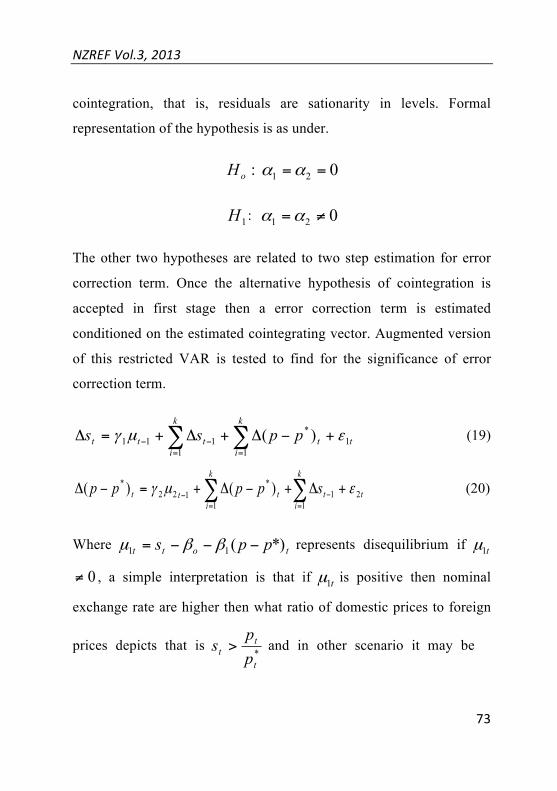
NZREF  Vol.3,  2013  

73  

cointegration, that is, residuals are sationarity in levels. Formal

representation of the hypothesis is as under.

:oH 021 ==αα

1H : 021 ≠=αα

The other two hypotheses are related to two step estimation for error

correction term. Once the alternative hypothesis of cointegration is

accepted in first stage then a error correction term is estimated

conditioned on the estimated cointegrating vector. Augmented version

of this restricted VAR is tested to find for the significance of error

correction term.

∑∑==

−− +−Δ+Δ+=Δk

itt

k

ittt ppss

11

*

1111 )( εµγ (19)

∑∑=

−=

− +Δ+−Δ+=−Δk

itt

k

ittt spppp

121

1

*122

* )()( εµγ (20)

Where tott pps *)(11 −−−= ββµ represents disequilibrium if t1µ

0≠ , a simple interpretation is that if t1µ is positive then nominal

exchange rate are higher then what ratio of domestic prices to foreign

prices depicts that is *t

tt p

ps > and in other scenario it may be

 NZREF  Vol.3,  2013    

74  

*t

tt p

ps < , the coefficient 1γ on lagged value of 1−tµ and 2γ on lagged

value of 12 −tµ essentially work to make *t

tt p

ps = and their seize and

significance matters for upholding the version of PPP theory

maintained is this paper. Further lagged values in the differences, that

is, 1−Δ ts and 1* )( −−Δ tpp describes at which lag along with error

correction term model given above may moves towards equilibrium.

Our null hypothesis is in this case correspond to a situation in which

1γ and 2γ both are equal to zero where as in alterative hypothesis is of

that at least one of them is not zero.

Such error correction terms defined above will certainly exist if

unrestricted augmented VAR of some order k , of change in ts that is

tsΔ and change in tpp )( *− which is tpp )( *−Δ on its level 1−ts

and 1* )( −− tpp and on its lagged changes is not a just a stationery

linear system in changes. This unrestricted VAR is not run under the

constraint to satisfy cointegration. The important distinction from a

usual first difference VAR is that levels of ts and tpp *)( − which

may be non-stationery series are included. Prima facie this makes little

sense but if both series are cointegrating then their levels in given

below unrestricted augmented VAR happens to be significant. This

NZREF  Vol.3,  2013  

75  

important property is taken as first step in Johanson Cointegration

approach. Augmented unrestricted VAR is represented as under.

∑∑==

−−− +−Δ+Δ+−+=Δk

itt

k

itttt ppsppss

11

*

111

*211 )()( εφφ (21)

∑∑=

−=

−− +Δ+−Δ+−+=−Δk

itt

k

itttt sppppspp

121

1

*1

*413

* )()()( εφφ (22)

Our null hypothesis may tell that unrestricted model is VAR of kth lags in changes such that levels don’t exist. It will be tested against alternative of significance of levels, if our alternatives hypothesis is found true then we are certain to find significant error correction term in restricted augmented VAR model given in equation (20) & (21). Usually an unrestricted augmented VAR is run first to estimate error correction model in the levels and in its changes and then these results are confirmed through restricted augmented VAR through equation (20) & (21).

4 Data

The data consists of monthly values from January 1980 to September 2009 for nominal exchange rate (Value of one unit of currency of the Sweden Krona in terms of the United States that is US$) and CPI indexes of both the countries. I have used the Exchange Rates between Sweden and USA and the Consumer Price Indices (CPI) of both the countries. The Exchange Rate data is downloaded from oanda.com. I took reciprocal of the exchange rate of ‘USA to Sweden’ to obtain the nominal exchange rate of ‘Sweden to USA’. The data for CPI of Sweden is obtained from the website of Statistiska Centralbyrån and that of USA is taken from the US Department of Labor, Bureau of Labor Statistics. Before, delving into some detailed computational

 NZREF  Vol.3,  2013    

76  

testing procedures, some of the simple characteristics of given data is analyzed through their descriptive statistics and correlation patterns. Further I investigated relationship between nominal and real exchange rates, and of real exchange rate, with relative prices, between two countries by plotting graphs between them. Doing so, may have further insight about the results. Firstly, a simple descriptive statistics are summarized as under.

Table 1 Descriptive Statistics

CPI

(SWE)

CPI

(US) */ tt PP

tS tQ

Mean 5.36 4.97 0.39 -1.96 -1.82

Median 5.52 5.01 0.41 -1.98 -1.83

Std. Deviation 0.32 0.27 0.08 0.19 0.17

Skewness -0.94 -0.32 -0.52 0.49 0.29

Kurtosis 2.62 2.03 2.71 3.63 3.15

Jarque-Bera 54.7 20.26 17.6 20.32 5.71

Simply speaking a mean of real exchange rate should remain near to 1 throughout the period under investigation so, that equality of aggregate price indexes of two countries in common currency is at first sight not established. Skewness is positive of the real, nominal exchange rates and relative prices, which means the distribution has a long right tail. Whereas CPI of both countries has a negative Skewness which implies

NZREF  Vol.3,  2013  

77  

the distribution has a long left tail. A graphical representation of same is attached figure-2 in appendix-I. In second step a pattern of correlations among variables of interest are presented as a table 3.

Table 2 Correlation Patterns CPI(SWE) CPI(USA) E Q

CPI(SWE) 1.00

CPI(USA) 0.966

E -0.508 -0.489

Q -0.451 -0.470 0.988 1.00

In above table a dissimilar pattern of correlation is easily observed, these are, however, static description of data but still vindicate that over span of data used in our study all variables are not tend to come closer to each and other. But on the other hand nominal exchange rate (E) and real exchange rate (Q) have negative correlation with CPI(SWE) and CPI(USA).To, Further understand our data, a graph between nominal and real exchange rates is presented in figure 2 in appendix-I.

 NZREF  Vol.3,  2013    

78  

5 Empirical Results This section presents empirical results for formulated problem statement of the paper.

5.1 Results from Unit Root Test In our data I have applied both ADF Test and Phillips Perron’s Test. Long run PPP is said to hold if the Real Exchange Rate sequence is stationary. Here I have constructed the Real Exchange Rate for Sweden trading Partner that is USA. To get the sequence of Real Exchange Rate (Q) .I have multiplied the Consumer Price Indices of USA to the Nominal Exchange Rate of Sweden to USA and then divided by the Consumer Price Indices of Sweden. The Log of the constructed series is the Real Exchange Rate sequence (Q).Using the ADF test and the Monthly Data of the synthetic real Krona/Dollar Exchange Rate for the selected period suggest that the real exchange rate is Non-Stationary. The results of ADF test reject the null hypothesis at all the three significant levels. This suggests that PPP not hold for the give period. A graphical representation of merits a brief discussion (Figure-4 in appendix-A). Graph of the real exchange rate is not stationary. The graph shows some upward and downward movement during this period. Also there is some Structural breaks during this period. If we look at the Correlogram we see that the ACFs are suffered from linear decline and there is only one significant spike of PACFs. To, further assure the non- sationarity of the series PP-test regression given in equation (8) was run. This time Rejection was even louder and our null hypothesis was rejected at 1%, 5% and 10% level of significance. The summary of results of ADF-test and PP-test are given in the below table.

NZREF  Vol.3,  2013  

79  

Table 3 ADF-Test and PP-Test for Real Exchange Rates

T-Statistics. 1% 5% 10%

ADF-Test. -2.35 -3.98 -3.42 -3.13

PP-Test. -2.39 -3.98 -3.427 -3.13

Note.   The   critical   values  MacKinnon   critical   values,   *  means   significance   at  1%  level  and  **  means  significance  at  5%  level  of  significance  

5.2 Cointegration Results The nominal exchange rate series ts and relative price series

tpp *)( − were checked for integration of same order, that is, if they

are I(1) processes. A regression in the change in nominal exchange rate

on its past level (ADF-test) gives a t-statistics of -2.426572 which

clearly show that it is not integrated of order one. Running the same

model with second difference on lagged first differences and 2nd

differences (ADF-test in first difference) gives the t-statistics of -

8.668604, indicating that first difference is stationery. The same

procedure is used for series of relative prices tpp *)( − the two test-

statistics are -2.307097  and -11.14824 respectively, again establishing

that relative prices are not cointegrated of the same order, hence there

is no tendency of mean reversion. So we conclude consequently an

absence of error correction term. This result is not surprising because

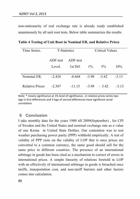
 NZREF  Vol.3,  2013    

80  

non-stationarity of real exchange rate is already ready established

unanimously by all unit root tests. Below table summarizes the results.

Table 4 Testing of Unit Root in Nominal ER, and Relative Prices

Time Series. T-Statistics Critical Values

ADF-test

Level.

ADF-test

1st Dif. 1% 5% 10%

Nominal ER. -2.426 -8.668 -3.98 -3.42 -3.13

Relative Prices -2.307 -11.15 -3.98 - 3.42 -3.13

Note:  *  means  significance  at  1%  level  of  significance  ,  in  relative  prices  series  two  lags  in  first  differences  and  3  lags  of  second  differences  have  significant  serial  correlation.  

6 Conclusion I take monthly data for the years 1980 till 2009(September) , for CPI of Sweden and the United States and nominal exchange rate as a value of one Krona in United State Dollars. Our contention was to test weather purchasing power parity (PPP) withhold empirically. A test of validity of PPP rests on the validity of LOP that is once prices are converted to a common currency, the same good should sell for the same price in different countries. The presence of an international arbitrage in goods has been cited as a mechanism to correct of errors in international prices. A simple linearity of relations foretold in LOP with an effectively of international arbitrage in goods is breached once tariffs, transportation cost, and non-tariff barriers and other factors comes into calculation.

NZREF  Vol.3,  2013  

81  

This paper is concern with the absence or presence of purchasing power parity for Sweden. The Sweden is taken as domestic country and United States of America is taken as foreign country. To check the absence or presence of PPP I check the statioarity and Non-stationarty of the real exchange rate. If the real exchange rate is stationary, it mean PPP hold otherwise do not hold. For this purpose I have used two different types of unit root tests that ADF test and Phillips Perron’s test. Both of these test has failed to find evidence in favour of purchasing power parity. Moreover, it is found that nominal exchange rates and price levels between Sweden and the United States are not cointegrated of the same order; hence there is no tendency of mean reversion. So I conclude consequently an absence of error correction term. This result is not surprising because non-stationarity of real exchange rate is already ready established unanimously by all unit root tests.

References

Abauf, Niso and P.Jorion.1990.” Purchasing Power Parity in the Long Run”, Journal of Finance, 45(1), pp.157-74.

Alder, Michael and Bruce Lehmann.1983.”Deviation from Purchasing Power Parity in Long Run”, Journal of Finance, 38(5), pp.1471-87.

Alba, Joseph D and Park Donghyun Park.2003.”Purchasing Power Parity in Developing Countries: Multi-Period Evidence under the Current Float”, World Development, 31(2), pp.2049-60.

Ardeni, Giorgio Pier and Lubian, Diego.1990. “Is there Trend Reversion in Purchasing Power Parity?” European Economic Review, 35,pp.1035-55.

Balassa, Bela.1964.”The Purchasing Power Parity Doctrine: A Reappraisal”, Journal of Political Economy, 72(6), pp.584-96.

 NZREF  Vol.3,  2013    

82  

Cheung, Yin-Wong and Lai, Kon S.1994. “Mean Reversion in Real Exchange Rates”, Economic Letters, 46(3), pp.251-56.

Davidson Russell and MacKinnon James G.1993. Estimation and Inference in Economics. New York Oxford: Oxford University Press.

Dickey, David A. and Fuller, Wayne 1979 “Distribution of the Estimators for Autoregressive Time Series with a Unit Root”, Journal of American Statistics, 74, pp.427-31.

Dornbusch, Rudiger.1976. “Expectations and Exchange Rate Dynamics”, Journal of Political Economics, 84(6), pp-1161-76.

Edison, Hali J. 1987.”Purchasing Power Parity in the Long Run: A Test of the Dollar/Pound Exchange rate (1890-1978)”, Journal of Money, Credit and Banking.19 (3), pp.376-87.

Edison, Hali J. and Klovland Jan Tore. “A Quantitative Reassessment of the Purchasing Power Hypothesis: Evidence from Norway and the United Kingdom”, Journal of Applied Econometrics, 2(4), pp.309-33.

Engle, Robert and Clive W.J.Granger.1987.” Co-integration and Error Correction: Representation, Estimation and Testing”, Econometrica, 55(2), pp.251-76.

Fisher, E. O. N. and Park, J. Y. (1991), “Testing Purchasing Power Parity under the Null Hypothesis of Cointegration,” The Economic Journal, 101, pp.1476-84.

Frankel, Jeffery A.1990.”Zen and the Art of Modern Macroeconomies: A Commentary,” in Monetary Policy for a Volatile Global Economy .W.S.Haraf and T.D.Willet, eds. Washington, D.C.: AEI Press, pp.117-23.

Friedman, Milton.1980. “Prices of Money and Goods Across Frontier: The £ and $ over a century” The World Economy, 2(1), pp.497-511.

NZREF  Vol.3,  2013  

83  

Gailliot, Henry J.1970. “Purchasing Power Parity as an Explanation of

Long-Term Changes in Exchange Rates.” Journal of Money, Credit

and Banking, 2(3), pp.348-57.

Giovannini, Alberto. 1988. “Exchange Rates and Traded Goods Prices”, Journal of International Economics, 24, pp.45-68.

Granger, Clive W.J. and P.Newbold. “Spurious Regression in Econometrics”, Journal of Econometrics, 2, pp.111-120.

Granger, Clive W.J. and Timo Teräsvirta.1993. Modelling Nonlinear Economic Relationships.Oxford: Oxford University Press.

Hakkio, C. (1984), “A Re-Examination of Purchasing Power Parity,” Journal of International Economics, 17, pp.265-77. Isard, Peter.1977. “How Far Can We Push the Law of One Price?” American Economic Review,67(5).pp.942-48.

Juselius, Katarina and Johansen, Soren.1990. ” Maximum Likelihood Estimation and Inference on Cointegration-With Application to the Demand for Money”, Oxford Bulletin of Economics and Statistics,52(2),pp-169-210.

Kwiatkowski, D., Phillips, P.C.B., Schmidt, P., and Shin, Y. (1992), “Testing the Null Hypothesis of Stationarity against the Alternative of a Unit Root,” Journal of Econometrics, 54, pp.159-78. Lee, Moon H.1976. Purchasing Power Parity. New York: Marcel Dekker, 1976.

Lothian, James R. and Mark P.Taylor.1996. “Real Exchange Rate Behaviour: The Recent Float From the Perspective of the Past Two Centuries”, Journal of Political Economy, 104(3), pp.488-509.

 NZREF  Vol.3,  2013    

84  

Murray, Christian J. and David H.Papell.2001.” The Purchasing Power Parity Persistence Paradigm” Journal of International Economics, 56(1), pp.1-19.

Oskooee,Bahmani M. and Nasir, ABM.2005.” Productivity Bias Hypothesis and the Purchasing Power Parity: A Review Article”, Journal of Economic Surveys, 19(4), pp.671-695.

Pakkio R.Michael and Pollard S.Patircia.2004. The Regional Economist.Retreived on March 16, 2006.www.stlouisfed.org.

Rogoff, Kenneth.1996. “The Purchasing Power Parity Puzzle”. Journal of Economic Literature. 34(2), pp.647-68.

Samuelson, Paul A.1964. “Theoretical Notes on Trade Problems”, Review of Economics and Statistics.46 (2), pp.145-54.

Taylor, Alan M.2002.” A Century of Purchasing Power Parity”, Review of economics and Statistics, 84(1), pp.139-50.

Taylor, Alan M. and Taylor, Mark P.2004. “The Purchasing Power Parity Debate”, Journal of Economic Perspective, 18(4), pp.135-158.

Taylor, Mark P., David A. Peel and Lucio Sarno .2001. “Nonlinear Mean-Reversion in Real Exchange Rates: Towards a Solution to Purchasing Power Parity Puzzles”, International Economic Review, 42(4), pp.1015-42.

Taylor, Mark P. and Lucio Sarno.1998. “The Behaviour of Real Exchange rates During the Post-Bretton Woods period”, Journal of International Economics, 42(2), pp.281-312.

 

 

NZREF  Vol.3,  2013  

85  

Appendix-I

Figure 1 Graph of real exchange rate

Figure 2 Change  in  Nominal  ER  with  Relative  Prices  

-2.4

-2.2

-2.0

-1.8

-1.6

-1.4

-1.2

1980 1985 1990 1995 2000 2005

ln Q

0.0

0.4

0.8

1.2

1.6

2.0

1980 1985 1990 1995 2000 2005

RP E

 NZREF  Vol.3,  2013    

86  

Figure 3 Movement of Nominal and real exchange rates

Figure 4 Patterns

.05

.10

.15

.20

.25

1980 1985 1990 1995 2000 2005

Q E

-3

-2

-1

0

1

2

3

4

5

6

1980 1985 1990 1995 2000 2005

Log of Price Level in SwedenLog of Price level in United StatesReal Exchange RatesLog of Nominal Exchange Rates

 NZREF  Vol.3,  2013    

 

87  

 

 

 

The Editorial Board of the New Zealand Review of Economics and Finance would like to extend our warm thanks to the Victoria Business School for financial and administrative support in publishing this edition of the journal. We also thank the Reserve Bank of New Zealand for providing prize money for the best article.

New Zealand Review of Economics and Finance Editorial Board

Managing Editors

Tahir Suleman

Editorial Board

Kay Winkler, Porntida Poontirakul

Faculty Advisors

Morris Altman, Chai-Ying Chang

New Zealand Review of Economics and Finance

Volume 3, 2013

In this issue:

Sodany Tong: The Changes to the New Zealand Top Personal Income Tax Policy between 2000-2010

Long Vo: An Overview of Development State in Thailand

Sodany Tong: The Evaluation of the New Zealand’s Electricity Market

Tahir Suleman: The Empirical Investigation of Long Run Purchasing Power Parity