Newton’s Method for Solving Non-Linear System of …article.sciencepublishinggroup.com/pdf/10.11648.j.ajmcm.20170204...Vol. 2, No. 4, 2017, ... This can be achieved by the aid of

American Journal of Mathematical and Computer Modelling 2017; 2(4): 117-131

http://www.sciencepublishinggroup.com/j/ajmcm

doi: 10.11648/j.ajmcm.20170204.14

Newton’s Method for Solving Non-Linear System of Algebraic Equations (NLSAEs) with MATLAB/Simulink

® and

MAPLE®

Aliyu Bhar Kisabo1, *

, Nwojiji Cornelius Uchenna2, Funmilayo Aliyu Adebimpe

3

1Department of Dynamics & Control System, Centre for Space Transport & Propulsion (CSTP), Lagos, Nigeria 2Department of Marine Engineering, Fleet Support Unit BEECROFT, Lagos, Nigeria 3Department of Chemical Propulsion System, Centre for Space Transport & Propulsion (CSTP), Lagos, Nigeria

Email address:

[email protected] (A. B. Kisabo) *Corresponding author

To cite this article: Aliyu Bhar Kisabo, Nwojiji Cornelius Uchenna, Funmilayo Aliyu Adebimpe. Newton’s Method for Solving Non-Linear System of Algebraic

Equations (NLSAEs) with MATLAB/Simulink® and MAPLE®. American Journal of Mathematical and Computer Modelling.

Vol. 2, No. 4, 2017, pp. 117-131. doi: 10.11648/j.ajmcm.20170204.14

Received: November 25, 2017; Accepted: December 7, 2017; Published: January 3, 2018

Abstract: Interest in Science, Technology, Engineering and Mathematics (STEM)-based courses at tertiary institution is on a

steady decline. To curd this trend, among others, teaching and learning of STEM subjects must be made less mental tasking.

This can be achieved by the aid of technical computing software. In this study, a novel approach to explaining and

implementing Newton’s method as a numerical approach for solving Nonlinear System of Algebraic Equations (NLSAEs) was

presented using MATLAB® and MAPLE

® in a complementary manner. Firstly, the analytical based computational software

MAPLE® was used to substitute the initial condition values into the NLSAEs and then evaluate them to get a constant value

column vector. Secondly, MAPLE® was used to obtain partial derivative of the NLSAEs hence, a Jacobean matrix.

Substituting initial condition into the Jacobean matrix and evaluating resulted in a constant value square matrix. Both vector

and matrix represent a Linear System of Algebraic Equations (LSAEs) for the related initial condition. This LSAEs was then

solved using Gaussian Elimination method in the numerical-based computational software of MATLAB/Simulink®

. This

process was repeated until the solution to the NLSAEs converged. To explain the concept of quadratic convergence of the

Newton’s method, power function of degree 2 (quad) relates the errors and successive errors in each iteration. This was

achieved with the aid of Curve Fitting Toolbox of MATLAB®. Finally, a script file and a function file in MATLAB

® were

written that implements the complete solution process to the NLSAEs.

Keywords: Newton’s Method, MAPLE®, MATLAB

®, Non-Linear System of Algebraic Equations

1. Introduction

The current decline in post-16 uptake of science,

technology, engineering and mathematics (STEM) subjects is

of great concern. The global consensus is that enrolment for

STEM studies and / or carriers has been in decline for more

than a decade.

One of the most frequently cited reasons for inspiring

young people to enjoy STEM are good teaching. The need

for quality teaching for students to become and remain

engaged in STEM cannot be over emphasized. As such,

innovative and inspirational teaching is needed now more

than ever to salvage the situation.

Perceived degree of difficulty-another commonly cited

reason in the extensive body of literature associated with the

switching young people off science is that STEM subjects are

perceived to be more difficult to achieve good grades than in

other subjects.

Another factor aiding the decline in STEM subjects is

unaccepted stereotypes about STEM. STEM, are associated

with being ‘boring’ and the perceptions that those who enjoy or

succeed in STEM subjects are, or might be, geeks or nerds.

Also, STEM based subjects are not seen to be ‘funky’ [1].

With affordable personal computers comes intuitive

STEM-based software like MATLAB® and MAPLE

®. Such

118 Aliyu Bhar Kisabo et al.: Newton’s Method for Solving Non-Linear System of Algebraic Equations (NLSAEs) with

MATLAB/Simulink® and MAPLE®

software goes a long way to address the factors cited above

responsible for the decline in STEM-based studies. Both

MATLAB® and MAPLE

® come with toolboxes and packages

respectively that ease a lot of the computation associated

with STEM subjects. An added edge which they both have is

powerful graphical visualization of results. This single

ingredient has greatly increased the understanding of STEM-

base subjects. The fact that certain scientific constants need

not to be memorized anymore but can be easily called for as

a built-in variable from such software is also a good omen for

STEM studies. These, with a lot more have reduced the

computational burden on the scientists.

Many STEM-based literatures have emerged that support

this understanding. We are not advocating a complete

substitution of the current methods of studying and teaching

STEM-based subject. The crux here is to complement the

existing methods. Taking a critical look into the future we

can boldly say, ‘Software will not replace STEM-based

teachers but teachers who do not use such software will soon

be replaced by those who do.’

For example, MAPLE® is used for purely analytical

solution processes in [2, 3, 4]. While areas where numerical

results are needed, MATLAB® is employed [4, 5, 6, 7]. The

combination of MATLAB®

and MAPLE® was used to

enforce understanding of both analytical and numerical

computations respectively in [8]. Though, both MATLAB®

and MAPLE® are capable of analytical and numerical

computation independently, their specific potential is greatly

harnessed when MATLAB® is used for numerical

computations and MAPLE® for analytical computation only.

In this study we intend to explore the numerical strength of

MATLAB®, and the analytical power of MAPLE

® to aid in

the understanding of the solution process of a NLSAEs using

Newton’s method.

This paper is divided in to the following sections; section

two defines terms associated with a system of nonlinear

algebraic equations, discusses the solution nature so desired

and the concept of convergence. In section 3, Newton’s

method was introduced and all the steps involve in using this

method to obtain solution to a NLSAEs were highlighted.

Section four presents an example and shows how Newton’s

method was applied using MATLAB® and MAPLE

® to

finally arrive at the required solution. Section five, presents

error analysis using curve fitting toolbox of MATLAB to

curve fit the errors from the numerical method used so far.

Finally, in section 6, MATLAB® script and function files

were written that implemented the Newton’s method for the

NLSAEs. Section seven concludes the study. A Laptop with

RAM 6.00GB, Intel(R) Core(TM) i5-2430M CPU @

2.40GHz, with windows 7, running MATLAB R2016a and

MAPLE 2015 versions was used throughout this study.

2. Nonlinear Algebraic Equations

Restricting our attention to algebraic equations in one

unknown variable, with pen and paper, one can solve many

types of equations. Examples of such equations are, ax+b =

0, and ax2+bx+c=0. One may also know that there are

formulas for the roots of cubic and quartic equations too.

Maybe one can do the special trigonometric equation sinx +

cosx = 1 as well, but there it (probably) stops. Equations that

are not reducible to one of those mentioned cannot be solved

by general analytical techniques. This means that most

algebraic equations arising in applications cannot be treated

with pen and paper!

If we exchange the traditional idea of finding exact

solutions to equations with the idea of rather finding

approximate solutions (numerical), a whole new world of

possibilities opens up. With such an approach, we can in

principle solve any algebraic equation [9].

An equation expressed by a function f as given in (1) is

defined as being nonlinear when it does not satisfy the

superposition principle as given in (2),

: nf →ℝ ℝ (1)

( ) ( ) ( )1 2 1 2f x x f x f x+ + ≠ + +⋯ ⋯ (2)

where ( )1 2, ,⋯ ℝn

nx x x ∈ and each fi is a nonlinear real

function, i = 1,2,…, n.

A system of nonlinear equations is a set of equations

expressed as the following:

( )( )

( )

1 1 2

2 1 2

1 2

, , 0,

, , 0,

, , 0,

⋯

⋯

⋮

⋯

n

n

n n

f x x x

f x x x

f x x x

=

=

=

(3)

A solution of a system of equations f1, f2, …, fn in n

variables is a point (a1, …, an) ℝn∈ such that f1(a1,…an) =

…

= fn (a1,…an) = 0.

Systems of Nonlinear Algebraic Equations cannot be

solved as nicely as linear systems. Procedures called iterative

methods are frequently used. An iterative method is a

procedure that is repeated over and over again, to find the

root of an equation or find the solution of a system of

equations. When such solution converges, the iterative

procedure is stopped hence, the numerical solution to the

system of equations.

Let F be a real function from D Є ℝn to ℝn . If F(p) = p,

for some p Є D, then p is said to be a fixed point of F.

Let pn be a sequence that converges to p, where pn ≠ p. If

constants λ, α > 0 exist that

1lim

n

nn

p p

p pα λ+

→∞

−=

− (4)

Then it is said that pn converges to p of order α with a

constant λ.

The value of α measures how fast a sequence converges.

Thus, the higher the value of α is, the more rapid the

convergence of the sequence is. In the case of numerical

methods, the sequence of approximate solutions is

American Journal of Mathematical and Computer Modelling 2017; 2(4): 117-131 119

converging to the root. If the convergence of an iterative

method is more rapid, then a solution may be reached in

fewer interactions in comparison to another method with a

slower convergence

3. Newton’s Method

The Newton-Raphson method, or Newton method, is a

powerful technique for solving equations numerically. It is

even referred to as the most powerful method that is used to

solve a nonlinear equation or system of nonlinear equations

of the form f(x) = 0. It is based on the simple idea of linear

approximation. The Newton’s method, properly used, usually

homes in on a root with devastating efficiency.

If the initial estimate is not close enough to the root,

Newton’s method may not converge, or may converge to the

wrong root. With proper care, most of the time, Newton’s

method works well. When it does work well, the number of

correct decimal places roughly doubles with each iteration.

In his Honors Seminar, Courtney Remani explained the

notion of numerical approximation very clearly, pointing to

the popular fact that Newton’s method has its origin in

Tailor’s series expansion of f(x) about the point x1:

21 1 1 1

1( ) ( ) ( ) ( ) ( ) ( )

2!⋯f x f x x x f x x x f x′ ′′= + − + − + (5)

where f, and its first and second order derivatives, f ′ and f ′′

are calculated at x1. If we take the first two terms of the

Taylor's series expansion, we have:

1 1 1( ) ( ) ( ) ( )f x f x x x f x′≈ + − (6)

Let (6) be set to zero (i.e. f(x) = 0) to find the root of the

equation which gives us:

1 1 1( ) ( ) ( ) 0.f x x x f x′+ − = (7)

Rearranging (7) we obtain the next approximation to the

root, as:

( )( )

11

1

,f x

x xf x

= −′

(8)

Thus, generalizing (8) gives the Newton’s iterative

method:

11

1

( ),

( )ℕ

ii i

i

f xx x i

f x

−−

−= − ∈

′ (9)

where xi → � ( as i → ∞), � is the approximation to a root of

the function f(x)

Note, as the iteration begins to have the same repeated

values i.e., as 1i ix x x+= = this is an indication that f(x)

converges to �. This xi is the root of the function f(x).

Another indicator that xi is the root of the function is if it

satisfies |�(��)| < ԑ, where ԑ > 0 is a given tolerance.

Newton’s method as given in (9) can only be used to solve

nonlinear equations with only a single variable. For a multi-

variable nonlinear equation, (9) has to be modified.

From Linear Algebra, we know that a system of equations

can be expressed in matrices and vectors. Considering a

multivariable system as expressed in (3), a modification of

(9) is written as:

( ) ( ) ( )( ) ( )( )11 1 1

x x x F xk k k k

J−− − −= − (10)

Where k = 1, 2, …, n represents the iteration, x Є ℝ , F is a

vector function, and J(x)-1

is the inverse of the Jacobian

matrix. However, to solve a system of nonlinear algebraic

equations instead of solving the equation f(x) = 0, we are now

solving the system F(x) = 0. Component of (10) are defined

as;

I. Let F be a function which maps nℝ to n

ℝ .

( )

( )( )

( )

1 1 2

2 1 21 2

1 2

, ,

, ,F , ,...,

, ,

⋯

⋯

⋮

⋯

n

nn

n n

f x x x

f x x xx x x

f x x x

=

(11)

where fi: n →ℝ ℝ .

II. Let x .ℝn∈ Then x represents the vector

1

2x=⋮

n

x

x

x

(12)

Where ix ∈ℝ and i = 1,2,…, n.

III. J(x) is the Jacobian matrix. Thus J(x)-1

is

( )

( ) ( ) ( )

( ) ( ) ( )

( ) ( ) ( )

1

1 1 1

1 2

2 2 21

1 2

1 1

x x x

x x x

x x x

⋯

⋯

⋮ ⋮ ⋯ ⋮

⋯

n

n

n n n

n

f f f

x x x

f f f

x x xJ x

f f f

x x x

−

−

∂ ∂ ∂ ∂ ∂ ∂ ∂ ∂ ∂ ∂ ∂ ∂=

∂ ∂ ∂ ∂ ∂ ∂

(13)

4. Solving an Example

Considering a system of three-nonlinear algebraic

equations [10] given in (14), solution to such system is

desired and we intend to use Newton’s method of

approximation.

( )

( )1 2

1 2 3

221 2 3

3

13 cos 0,

2

81 0.1 sin 1.06 0,

10 320 0,

3

x x

x x x

x x x

e xπ−

− − =

− + + + =−+ + =

(14)

The graphing facilities of MAPLE® can assist in finding



initial approximations to the solutions of 2 × 2 and often 3 ×

3 nonlinear systems. To do this, we need to input (14) in a

MAPLE® worksheet. MAPLE

® has in-built Palettes that can

assist. These are highlighted in Figure 1.

Figure 1. MAPLE window with Palettes highlighted.

The following were used to insert the first nonlinear equation in (14), and its plot is as depicted in Figure 2.

( )( )

( ) ( )

( )( )

:

g :

:

1: , , 3 cos , ;

2

: 3 , , 0, 0..2, 0..2, 2..2, , [2,2,2] ;

restart

with linal

with plots

f x y z x x y

plotf implicitplot d f x y z x y z color red grid

= → ⋅ − −

= = = = = − = =

Figure 2. Plot for ( )1 2 31

3 cos 02

x x x− − = .

Notice that the unknown variables x1, x2, and x3 in (14)

have been substituted with x, y, z respectively in the code that

was fed into MAPLE®. This was done to accommodate the

function assignment. To continue with the plot of the second

equation, the following were added to the worksheet:

( ) ( ) ( )( )( )

22: , , 81 y 0.1 sin 1.06;

: 3 , , 0, 0..2, 0..2, 2..2, , [2,2,2] ;

g x y z x z

plotg implicitplot d g x y z x y z color blue grid

= → − + + +

= = = = = − = =

Figure 3. Plot for ( )221 2 381 0.1 sin 1.06 0,x x x− + + + = .


To also visualize the third equation, the following MAPLE® code gave Figure 4:

( ) ( )

( )( )

10 3: , , 20 ;

3

: 3 , , 0, 0..2, 0..2, 2..2, , [2,2,2] ;

x yh x y z e z

ploth implicitplot d h x y z x y z color yellow grid

π− ⋅ ⋅ −= → + ⋅ +

= = = = = − = =

Figure 4. Plot for 1 23

10 320 0,

3

x xe xπ− −+ + = .

Finally, to combine the three plots (Figure 2, Figure 3, and

Figure 4) on the same axis, we typed:

{ }( ), , , , ;display plotf plotg ploth axes boxed scaling constrained= =

Figure 5. Plot for NLSAEs as given in (13).

From Figure 2 to Figure 5, particularly after zooming and

rotating Figure 5, we agree that an initial guess of the

solution to (14) as given in (15) is a good one.

( )0

0.1

0.1 .

0.1

x

= −

(15)

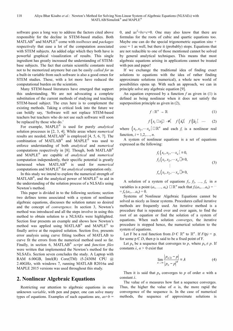
Note, (15) is the first step for solving (14) using Newton’s

method. The second step is to define F(x) as,

( )

( )

( )1 2

1 2 3

221 2 3

3

13 cos

2

F x 81 0.1 sin 1.06 ,

10 320

3

x x

x x x

x x x

e xπ−

− − = − + + +

− + +

(16)

To evaluate F(x(0)

) is the third step. This involves

substituting and evaluating (16) with (15), here we used

MAPLE® [11, 12] to achieve our goal. Palettes in MAPLE

®

as highlighted in red in Figure 1, were used. These Palettes

make entering expressions in familiar notation easier and

reduces the possibility of introducing typing errors.

( ) ( ) ( ) ( )( )( ): , , , , , , , , , , :

0.1,0.1, 0.1 ;

F x y z vector f x y z g x y z h x y z

F

= →

−

Note that after executing the above expressions in

MAPLE®, we got a row vector, since we know that what we

need is a column vector (transpose of the row vector) we

simply present it as;

( )( )0

1.19995

2.26983

8.46203

F x

− = −

(17)

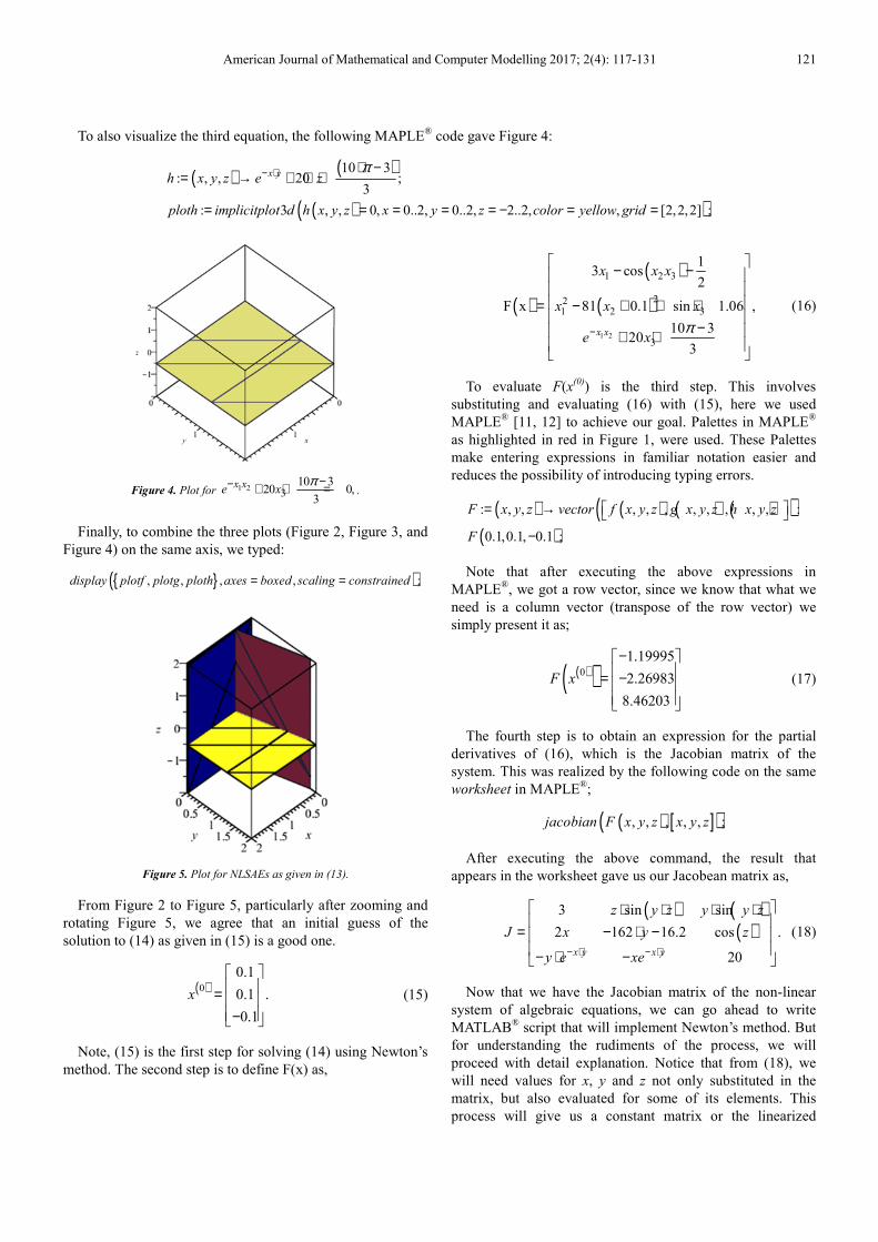
The fourth step is to obtain an expression for the partial

derivatives of (16), which is the Jacobian matrix of the

system. This was realized by the following code on the same

worksheet in MAPLE®;

( ) [ ]( ), , , , , ;jacobian F x y z x y z

After executing the above command, the result that

appears in the worksheet gave us our Jacobean matrix as,

( ) ( )( )

3 sin sin

2 162 16.2 cos .

20x y x y

z y z y y z

J x y z

y e xe− ⋅ − ⋅

⋅ ⋅ ⋅ ⋅

= − ⋅ − − ⋅ −

(18)

Now that we have the Jacobian matrix of the non-linear

system of algebraic equations, we can go ahead to write

MATLAB® script that will implement Newton’s method. But

for understanding the rudiments of the process, we will

proceed with detail explanation. Notice that from (18), we

will need values for x, y and z not only substituted in the

matrix, but also evaluated for some of its elements. This

process will give us a constant matrix or the linearized



version of the NLSAEs at the given initial condition. This

would be the fifth step. Two ways of doing such will be

presented here. First, in MAPLE® each element of (18) will

be defined as a function followed by substitution and

evaluation of the function will be done by the given initial

value. Hence:

1,1 : 3;j =

Note that j1,1 is already a constant value of the Jacobean

matrices in (18). To obtain the second element on the first

row it will require the substitution of variable and evaluation

of the expression. This was achieved by the following codes

in the same MAPLE® worksheet;

( )( )( )

1,2

1,2 12

: sin ;

: 0.1, 0.1,

f z y z

j eval sub y z f

= ⋅ ⋅

= = = −

Hence j1,2 is the second element on the first row. To proceed,

we simply copy and paste expression in MAPLE® and modify

variables where necessary. The remaining codes are;

Figure 6. MAPLE window showing the matrix Pallet.

( )( )( )

( )( )

( )( )( )

1,3

1,3 13

2,1

2,1 2,1

2,2

2,2 2,2

2,3

: sin ;

: 0.1, 0.1,

: 2 ;

: 0.1,

: 162 16.2;

: 0.1,

: cos ;

f y y z

j eval sub y z f

f y

j eval sub y f

f y

j eval sub y f

f z

= ⋅ ⋅

= = = −

= ⋅

= =

= − ⋅ −

= =

=

( )( )

( )( )

( )( )

2,3 23

3,1

3,1 3,1

3,2

3,2 3,2

3,3

: 0.1,

: ;

: 0.1, 0.1,

: ;

: 0.1, 0.1,

: 20;

xy

xy

j eval sub z f

f y e

j eval sub x y f

f x e

j eval sub x y f

j

−

−

= = −

= − ⋅

= = =

= − ⋅

= = =

=

Hence, J(x(0)

) is given by inserting a 3x3 matrix from the

matrix pane of MAPLE® (Figure 6) with description as;

1,1 1,2 1,3

2,1 2,2 2,3

3,1 3,2 3,3

:not

j j j

J j j j

j j j

=

After execution, the above MAPLE® syntax, the realized

J(x(0)

) is,

( )( )0

3 0.00099 0.00099

0.2 32.4 0.99500 .

0.09900 0.09900 20

J x

− = − − −

(19)

The second approach of getting (19) in MAPLE®

is by

reverting back to the form in which (14) is presented, i.e.,

designating the unknown variable as x1, x2 and x3:

( )

( ) ( ) ( ) ( ) [ ] [ ]1 222

1 2 3 1 2 3 3 1 2 3

:

10 313 cos , 81 0.1 sin 1.06, 20 , , , 0.1,0.1, 0.1 ;

2 3

x x

with VectorCalculus

Jacobian x x x x x x e x x x xπ− ⋅ ⋅ −

⋅ − ⋅ − − + + + + ⋅ + = −


At this stage, the linearization of the (14) with initial

values as given in (15) is completed and in concise matrix

form we can write the linearized system as;

( )( ) ( ) ( )( )0 0 0,J x y F x= − (20)

where (0) (0)(0) (0)1 2 ⋯

T

ny y y y = is the solution to the

linear system of algebraic equations.

At this stage a comprehensive MAPLE®

worksheet has

been successfully developed for the first iteration. This

worksheet will be used for subsequent iterations.

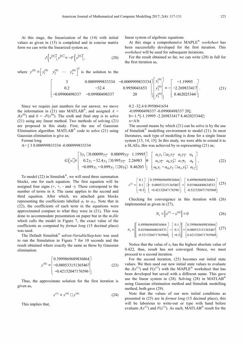
For the result obtained so far, we can write (20) in full for

the first iteration as,

(0)1

(0)2

(0)3

3 0.0009999833334 0.0009999833334 1.19995

0.2 32.4 0.9950041653 2.269833417 .

0.09900498337 0.09900498337 20 8.462025344

y

y

y

− − − = − − − −

(21)

Since we require just numbers for our answer, we move

the information in (21) into MATLAB®, and assigned A =

J(x(0)

) and b = -F(x(0)

). The sixth and final step is to solve

(21) using any linear method. Two methods of solving (21)

are proposed in this study. First, the use of Gaussian

Elimination algorithm. MATLAB® code to solve (21) using

Gaussian elimination is give as;

Format long

A= [ 3 0.000999833334 -0.000999833334

0.2 -32.4 0.9950041654

-0.09900498337 -0.09900498337 20];

b=-1.*[-1.19995 -2.269833417 8.462025344]';

x=A\b

The second means by which (21) can be solve is by the use

of Simulink® modelling environment to model (21). In most

literatures, such type of modelling is done for a single linear

system [13, 14, 15]. In this study, we were able to extend it to

a SLAEs, this was achieved by re-representing (21) as;

( )1 2 3 1 1 2 2 3 3 4

1 2 3 5 1 6 2 7 3 8

1 2 3 9 1 10 2 11 3 12

3 0.00099 0.00099 1.19995

0.2 32.4 0.995 2.26983 ,

0.099 0.099 20 8.46203

y y y a y a y a y a

G x y y y a y a y a y a

y y y a y a y a y a

+ − − + − − = − + − ≡ − + − − − + + − + +

(22)

To model (22) in Simulink®, we will need three summation

blocks, one for each equation. The first equation will be

assigned four signs (+, +, - and -). These correspond to the

number of terms in it. The same applies to the second and

third equation. After which, we attached gain blocks

representing the coefficients labelled a1 to a12. Note that in

(22), the coefficients of each term in the equations were

approximated compare to what they were in (21), This was

done to accommodate presentation on paper but in the m-file

which calls the model in Figure 7, the exact value of the

coefficients as computed by format long (15 decimal place)

was used.

The Default Simulink® solver-VariableStepAuto was used

to run the Simulation in Figure 7 for 10 seconds and the

result obtained where exactly the same as those by Gaussian

elimination:

(0)

0.3999869689836864

0.080533151365467

0.42152047176596

y

= − −

(23)

Thus, the approximate solution for the first iteration is

given as,

(1) (0) (0)x x y= + (24)

This implies that,

(1)

0.1 0.3999869689836864 0.499869689836864

0.1 0.080533151365467 0.019466848634533

0.1 0.42152047176596 -0.521520471765960

x

= + − = − −

(25)

Checking for convergence in this iteration with (26)

implemented as given in (27),

(1) (0)1 0N x x= − = (26)

1

0.499869689836864 0.1 0.399869689836864

0.019466848634533 0.1 0.080533151365467

-0.521520471765960 0.1 0.421520471765960

N

= − = −

(27)

Notice that the value of x3 has the highest absolute value of

0.422, thus, result has not converged. Hence, we must

proceed to a second iteration.

For the second iteration, (25) becomes our initial state

values. We then used our new initial state values to evaluate

the J(x(1)

) and F(x(1)

) with the MAPLE® worksheet that has

been developed but saved with a different name. This gave

use the linear system in (28). Solving (28) in MATLAB®

using Gaussian elimination method and Simulink modelling

method, both gave (29).

Note that the values of our new initial conditions as

presented in (25) are in format long (15 decimal place), this

will be laborious to write-out or type with hand before

evaluate J(x(1)

) and F(x(1)

). As such, MATLAB® result for the



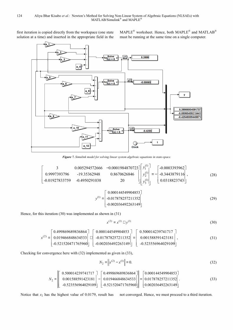
first iteration is copied directly from the workspace (one state

solution at a time) and inserted in the appropriate field in the

MAPLE® worksheet. Hence, both MAPLE

® and MATLAB

®

must be running at the same time on a single computer.

Figure 7. Simulink model for solving linear system algebraic equations in state-space.

(1)1

(1)2

(1)3

3 0.005294572666 0.0001984870723 -0.0003393962

0.9997393796 -19.35362948 0.8670626846 -0.3443879116 ,

-0.01927833759 -0.4950291038 20 0.0318823743

y

y

y

− = −

(28)

(1)

0.000144549904853

-0.017878257211352

-0.002036492263149

y

=

(29)

Hence, for this iteration (30) was implemented as shown in (31)

(2) (1) (1)x x y= + (30)

(2)

0.499869689836864 0.000144549904853 0.500014239741717

0.019466848634533 -0.017878257211352 0.001588591423181 ,

-0.521520471765960 -0.002036492263149 -0.523556964029109

x

= + =

(31)

Checking for convergence here with (32) implemented as given in (33),

(2) (1)2 0.N x x= − = (32)

2

0.500014239741717 0.499869689836864 0.000144549904853

0.001588591423181 0.019466848634533 0.017878257211352 .

-0.523556964029109 -0.521520471765960 0.002036492263149

N

= − =

(33)

Notice that x2 has the highest value of 0.0179, result has not converged. Hence, we must proceed to a third iteration.


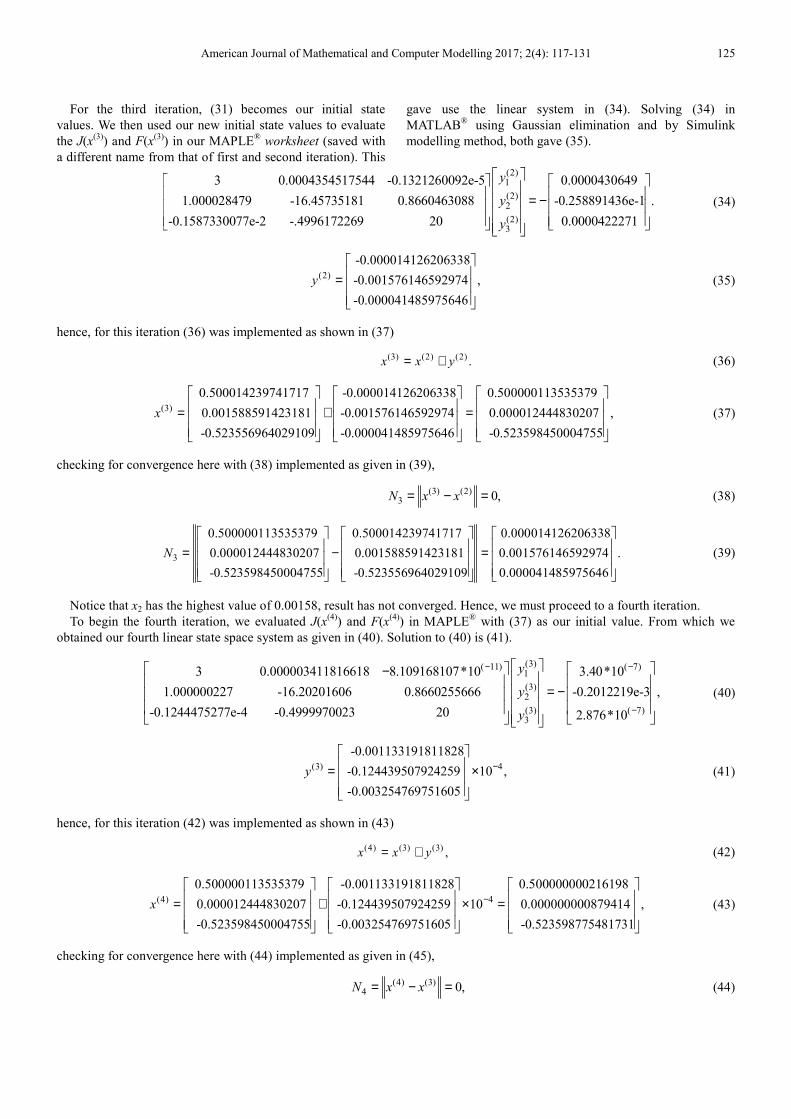
For the third iteration, (31) becomes our initial state

values. We then used our new initial state values to evaluate

the J(x(3)

) and F(x(3)

) in our MAPLE® worksheet (saved with

a different name from that of first and second iteration). This

gave use the linear system in (34). Solving (34) in

MATLAB® using Gaussian elimination and by Simulink

modelling method, both gave (35).

(2)1

(2)2

(2)3

3 0.0004354517544 -0.1321260092e-5 0.0000430649

1.000028479 -16.45735181 0.8660463088 -0.258891436e-1 .

-0.1587330077e-2 -.4996172269 20 0.0000422271

y

y

y

= −

(34)

(2)

-0.000014126206338

-0.001576146592974 ,

-0.000041485975646

y

=

(35)

hence, for this iteration (36) was implemented as shown in (37)

(3) (2) (2) .x x y= + (36)

(3)

0.500014239741717 -0.000014126206338 0.500000113535379

0.001588591423181 -0.001576146592974 0.000012444830207

-0.523556964029109 -0.000041485975646 -0.523598450004755

x

= + =

,

(37)

checking for convergence here with (38) implemented as given in (39),

(3) (2)3 0,N x x= − = (38)

3

0.500000113535379 0.500014239741717 0.000014126206338

0.000012444830207 0.001588591423181 0.001576146592974 .

-0.523598450004755 -0.523556964029109 0.000041485975646

N

= − =

(39)

Notice that x2 has the highest value of 0.00158, result has not converged. Hence, we must proceed to a fourth iteration.

To begin the fourth iteration, we evaluated J(x(4)

) and F(x(4)

) in MAPLE® with (37) as our initial value. From which we

obtained our fourth linear state space system as given in (40). Solution to (40) is (41).

(3)1

(3)2

(3)3

( 11) ( 7)

( 7)

3 0.000003411816618

1.000000227 -16.20201606 0.8660255666 -0.2012219e-3 ,

-0.1244475277e-4 -0.4999

8.109168107*10 3.40*10

2.876970023 20 *10

y

y

y

− −

−

= −

− (40)

(3) 4

-0.001133191811828

-0.124439507924259 10 ,

-0.003254769751605

y − = ×

(41)


(4) (3) (3) ,x x y= + (42)

(4) 4

0.500000113535379 -0.001133191811828 0.500000000216198

0.000012444830207 -0.124439507924259 10 0.000000000879414

-0.523598450004755 -0.003254769751605 -0.523598775481731

x − = + × =

,

(43)


(4) (3)4 0,N x x= − = (44)



4

0.500000000216198 0.500000113535379 0.001133191811498

0.000000000879414 0.000012444830207 0.124439507924259 10

-0.523598775481731 -0.523598450004755 0.003254769751493

N

= − = ×

4.− (45)

Notice that x2 has the highest value of 0.124 x 10-4

, result has not converged. Hence, we must proceed to a fifth iteration.

To begin the fifth iteration, we evaluated J(x(5)

) and F(x(5)

) in MAPLE® with (43) as our initial value. From which we

obtained our fifth linear state space system as given in (46). Solution to (46) by Gaussian Elimination method in MATLAB®

and Simulink® modelling method gave (47).

( 9)( 10) ( 19)

( 8)

(

(

10) ( 10

4)1

(4)2

( )4)3

3

1.000000000 -16.20000014 0.8660254038 ,

-.5

1.0 102.410963412 10 4.049350528 10

1.45 10

8.7941399 000000000 296 10 4. 10 0

y

y

y

−− −

−

− −

= −

×× − ×− ×

− ×

−

×

(46)

(4) 9

-0.333333333259735

-0.915792604227302 10 ,

-0.002894815120339

y − = ×

(47)


(5) (4) (4) ,x x y= + (48)

(5) 9

0.500000000216198 -0.333333333259735 0.499999999882865

0.000000000879414 -0.915792604227302 10 -0.000000000036379

-0.523598775481731 -0.002894815120339 -0.523598775484625

x − = + × =

,

(49)


(5) (4)5 0,N x x= − = (50)

5

0.499999999882865 0.500000000216198 0.333333360913457

-0.000000000036379 0.000000000879414 0.915792604227302

-0.523598775484625 -0.523598775481731 0.002894795514408

N

= − = ×

910 .− (51)

From (51), all values of x gave values after a decimal point

with at least nine zeros. This also means that there is no

difference between x(5)

and x(4)

. Hence, our result has

converged. Also, from the result of F(x(5)

) in (46), it could be

clearly seen that the x(5)

is the root of the system because

F(x(5)

) = 0.

Thus, the result obtained so far, i.e., values of x (equation

(25), (31), (37), (43), (49)) and N (equations (27), (33), (39),

(45), (51)) for iterations 1-5 can be summarized as given in

Table 1.

Table 1. Result of Newton’s method.

n ( )1

nx ( )

2n

x ( )3n

x nN (Error)

0 0.100000000000000 0.100000000000000 -0.100000000000000 -

1 0.499869689836864 0.019466848634533 -0.521520471765960 0.421520471765960

2 0.500014239741717 0.001588591423181 0.523556964029109 0.017878257211352

3 0.500000113535379 0.000012444830207 -0.523598450004755 0.001576146592974

4 0.500000000216198 0.000000000879414 -0.523598775481731 0.0000124439507924259

5 0.499999999882865 0.000000000036379 -0.523598775484625 0.0000000000028947955

5. Analysing Quadratic Convergence

The rate of convergence of the Newton’s method is often

“explained” by saying that, once you have determined the digit

in the first decimal place, successive iteration in a quadratic

convergent process roughly doubles the number of correct

decimal places. To a large extent, this explanation is vague.

Most mathematicians often come away with only the shortcut

explanation of how quadratic convergence compare in terms of

the number of correct decimal places obtained with each

successive iteration. Because numerical methods are assuming a

growing role in STEM courses and are being taught by people


having little, if any, training in numerical analysis, it is useful to

see this underlying idea expanded in greater detail.

Literatures on numerical analysis, such as [16, 17] provide

only technical explanation as part of formal derivations and

display only the successive approximations based on a

method, but tend not to look at the values of the associated

errors.

However, an analysis of the behavior of the errors in the

sense of data analysis and curve fitting provides a very

effective way to come to an understanding of the patterns of

convergence. Data analysis in the sense of fitting functions to

data has become a powerful mathematical idea introduced to

enhance the understanding of the concepts of convergence.

There are two ways to curve fit data in MATLAB [18].

First, method is by the use of the interactive curve fitting

Tool (an app).

Table 2. Iteration and Error Values.

S/N Iteration(n) Error

1 0 -

2 1 0.422

3 2 0.0179

4 3 0.00158

5 4 0.0000124

6 5 0

With this method your start the curve-fitting tool from the

app window by double clicking on the MATLAB® app for

curve fitting. The data in Table 2 (extracted from Table 1),

can then be entered as variables in vector form using the

command window.

In our case, the power function best fit our data and

directly below it is the number of terms option for this

function. This was left at the value of 1 because from the

results window (Figure 8, lower left corner) the Goodness of

fit has acceptable values.

After using graphical methods to evaluate how well the

fitted curve matches our data, we further examined the

numerical values attached to the goodness-of-fit statistics,

these are;

I. Sum of Squares Due to Error (SSE). This statistic

measures the total deviation of the response values from the

fit. In simple words, SSE indicates how far data is from the

regression line. It is also called the summed square of

residuals, mathematically, it is represented as,

( )2

1

ˆn

i i i

i

SSE w y y

=

= −∑ (52)

where wi is the weighted of the function, y is the measured

value (data) and y is the predicted value (fitted curve).

II. R-Square. This statistic measures how successful the fit

is in explaining the variation of the data. Put another way, R-

square is the square of the correlation between the response

values and the predicted response values. It is also called the

square of the multiple correlation coefficient and the

coefficient of multiple determination.

R-square is defined as the ratio of the sum of squares of

the regression (SSR) and the total sum of squares (SST).

Mathematically, SSR is expressed as,

( )2

1

ˆn

i i

i

SSR w y y

=

= −∑ (53)

where y is the mean of values or measured data.

SST is also called the sum of squares about the mean, and

is defined as,

( )2

1

n

i i

i

SST w y y

=

= −∑ (54)

where SST = SSR + SSE. Given these definitions, R-square is

expressed as,

R-square = 1SSR SSE

SST SST= − (55)

III. Degrees of Freedom Adjusted R-Square. This statistic

uses the R-square statistic defined above, and adjusts it based

on the residual degrees of freedom. The residual degrees of

freedom are defined as the number of response values n

minus the number of fitted coefficients m estimated from the

response values.

v n m= − (56)

v indicates the number of independent pieces of

information involving the n data points that are required to

calculate the sum of squares. Mathematically, this is

expressed as,

( )( )

1adjusted R-square = 1

SSE n

SST v

−− (57)

IV. Root Mean Squared Error. This statistic is also known

as the fit standard error and the standard error of the

regression. It is an estimate of the standard deviation of the

random component in the data, and is defined as,

RMSE s MSE= = (58)

where MSE is the mean square error or the residual mean

square.

SSEMSE

v= (59)

From Figure 8, the power function for the fitted curve is as

given in (60) and the plot from Figure 8 can be extracted and

presented as given in Figure 9. Observe that the errors as

shown in Figure 9 clearly depict a pattern that suggests a

decaying function.



Figure 8. Interactive Curve Fitting GUI of MATLAB, error data and the fitted curve.

Figure 9. Interactive curve fitting app plot of data and fitted curve.

,bError a n= ⋅ (60)

where, a = 0.4215, n = number of iterations and b = -4.588.

The Goodness of fit attributes for (60) are; SSE = 2.032e-06,

this means that (60) has a small random error. R- square =1,

meaning 100% of the variance of the data in Table 2 is

accounted for by (60). RMSE = 0.0008231, this tells us that

(60) is good for predicting the data. Adjusted R-square = 1,

means that the fit explains 100% of the total variation in the

data about the average hence, (60) is perfect for prediction.

The second method of curve fitting a data in MATLAB® is

by writing out commands or MATLAB® codes. To reproduce

the fitted curve in Figure 9, in our case, we simply ran the

following MATLAB® code;

n=[1 2 3 4 5 ]'; Err=[0.422 0.0179 0.00158 0.0000124 0]'; f_o=fit(n, Err,'power1') plot(f_o,'predobs,95')

Note that in the above code, the variables have to be

entered as column vectors. With the interactive curve fitting

tool, variables were accepted as row vectors.

Figure 10. Plot of fitted curve with prediction bonds using MATLAB code.

Next, we will consider how each succeeding error value

En+1 compares to the current one En, as shown in Figure 11.

Table 3. Error and successive error values.

S/N En En+1

1 0.422 0.0179

2 0.0179 0.00158

3 0.00158 0.0000124

4 0.0000124 0

In Figure 11, we see that the data appear to be linear

(polynomial of first order). However, a closer examination of

how the points match the regression line we found that the

successor error En+1 is roughly proportional to the current

error En. This suggests the possibility that, when the

Err

or


convergence is quadratic, En+1, may be roughly proportional

to En. To investigate into this possibility, we perform a power

function regression on the values of En+1 versus those of En

(as given in Table 3) and found that the resulting power

function is,

1 ,bn nE a E c+ = ⋅ + (61)

where a = 0.07224, b = 1.649 and c = 0.0004968.

The Goodness of fit attributes for (61) are; SSE = 1.46e-

06, meaning that the random error component of (61) is very

small. R- square =0.9936. This informs us that 99.36% of the

variance of the data in Table 3 is accounted for by (61).

RMSE = 0.001208, this value is very close to zero hence,

(61) will be useful in predicting the data in Table 3. Adjusted

R-square = 0.9808. This R-square value indicates that the fit

explains 98.08% of the total variation in the data about the

average.

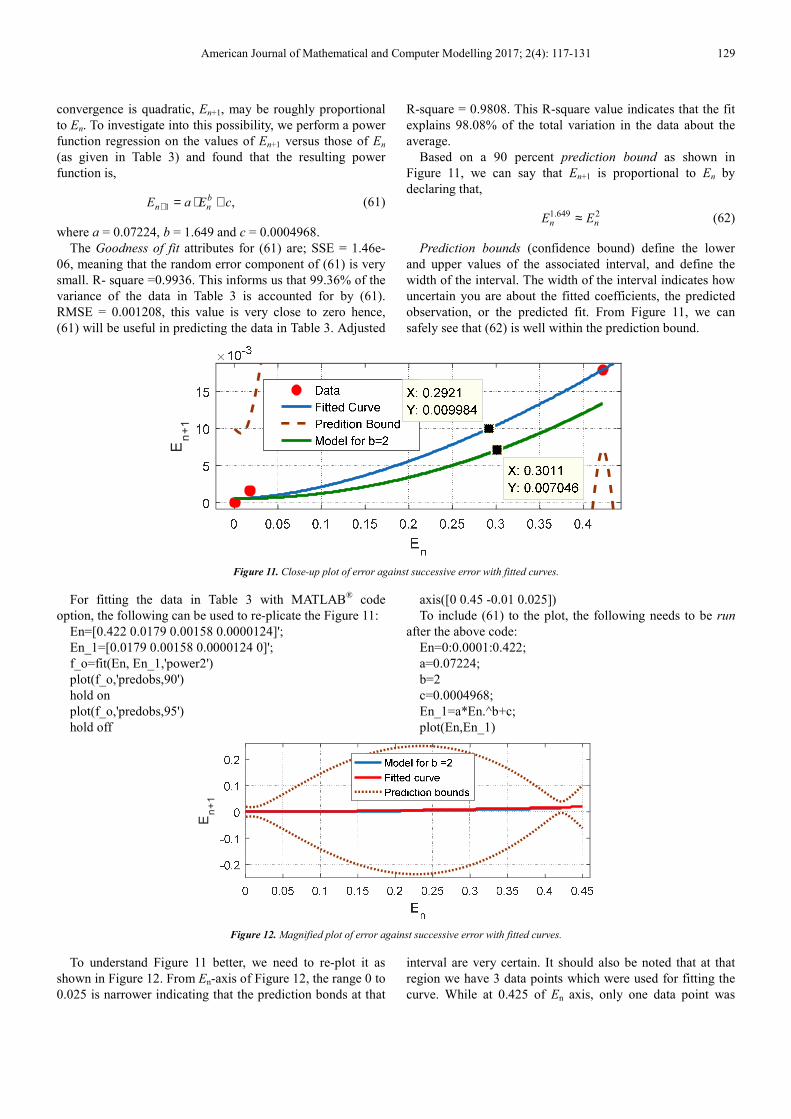
Based on a 90 percent prediction bound as shown in

Figure 11, we can say that En+1 is proportional to En by

declaring that,

1.649 2n nE E≈ (62)

Prediction bounds (confidence bound) define the lower

and upper values of the associated interval, and define the

width of the interval. The width of the interval indicates how

uncertain you are about the fitted coefficients, the predicted

observation, or the predicted fit. From Figure 11, we can

safely see that (62) is well within the prediction bound.

Figure 11. Close-up plot of error against successive error with fitted curves.

For fitting the data in Table 3 with MATLAB® code

option, the following can be used to re-plicate the Figure 11:

En=[0.422 0.0179 0.00158 0.0000124]'; En_1=[0.0179 0.00158 0.0000124 0]'; f_o=fit(En, En_1,'power2')

plot(f_o,'predobs,90')

hold on

plot(f_o,'predobs,95')

hold off

axis([0 0.45 -0.01 0.025])

To include (61) to the plot, the following needs to be run

after the above code:

En=0:0.0001:0.422; a=0.07224; b=2 c=0.0004968; En_1=a*En.^b+c; plot(En,En_1)

Figure 12. Magnified plot of error against successive error with fitted curves.

To understand Figure 11 better, we need to re-plot it as

shown in Figure 12. From En-axis of Figure 12, the range 0 to

0.025 is narrower indicating that the prediction bonds at that

interval are very certain. It should also be noted that at that

region we have 3 data points which were used for fitting the

curve. While at 0.425 of En axis, only one data point was

En

+1

En

+1



used for fitting the curve, and this point has the perdition

bonds closer to it too. This is indicating certainty of the

prediction at just that point. Unfortunately, the largest region

(from 0.025 to 0.4 on En-axis) of the fitted curve is very

uncertain for any form of prediction because no data exist at

this region. Hence, prediction within this region is not

certain. Luckily for us, we can barely notice the difference

between the two curves of (61) and (62) in Figure 12. This is

because the approximation is close enough. It is only in a

magnified plot as shown in Figure 11 that one could

differentiate visually between the two curves.

6. Matlab® Codes for Newton’s Method

After an intuitive understanding of a mathematical process

like the Newton’s method as presented in this study, a

contemporary researcher will quickly want to write a computer

program for it. The primary aim for doing such is for subsequent

use to solve similar problems with relative easy.

This program must be concise, easy to understand and of

few lines as possible. As such, in this study, two MATLAB®

programs were used to implement the entire Newton’s

method. The first program is written in an m-file. After

executing the program, convergence of the solution can be

judged by human examination of the result displayed at the

command window. This solution method uses the idea of

convergence as it relates to evaluating the norm for every

iteration, as explained earlier in this study.

% Newton's Method format long; n=5; % set some number of iterations, may need adjusting f = @(x) [ 3*x(1)-cos(x(2)*x(3))-0.5 x(1).^2-81*(x(2)+0.1)^2 + sin(x(3))+1.06 exp(-x(1)*x(2))+20*x(3)+((10*pi-3)/3)]; % the vector

function,3x1 % the matrix of partial derivatives df = @(x) [3 x(3)*sin(x(2)*x(3)) x(2)*sin(x(2)*x(3)) 2*x(1) -162*x(2)-16.2 cos(x(3)) -x(2)*exp(x(1)*x(2)) -x(1)*exp(x(1)*x(2)) 20];% 3x3 x = [0.1;0.1;-0.1]; % starting guess for i = 1:n y = -df(x)\f(x) % solve for increment, similar A\b x = x + y % add on to get new guess f(x) % see if f(x) is really zero end

The second MATLAB® program that implements the

Newton’s method for this study uses four function files of

MATLAB®. The first file carries the description for (16), a

vector of the functions:

function y = F(x) x1 = x(1); x2 = x(2); x3 = x(3); y = zeros(3,1); y(1) = 3*x(1)-cos(x(2)*x(3))-0.5; % f1(x1,x2) y(2) = x(1).^2-81*(x(2)+0.1)^2 + sin(x(3))+1.06; y(3) = exp(-x(1)*x(2))+20*x(3)+((10*pi-3)/3);

end

To solve the 5 LSAE in each iteration, a second function-

file that implement (18)-the Jacobian matrix is needed. The

Jacobian was computed in MAPLE® and the result serves as

the main input of the file.

function y = F(x) x1 = x(1); x2 = x(2); x3 = x(3); y = zeros(3,1); y(1) = 3*x(1)-cos(x(2)*x(3))-0.5; % f1(x1,x2); y(2) = x(1).^2-81*(x(2)+0.1)^2 + sin(x(3))+1.06; y(3) = exp(-x(1)*x(2))+20*x(3)+((10*pi-3)/3); end

A third file was written to implements the algorithm of the

Newton’s method with a given tolerance (1e-5) to indicate

that the solution has converged and immediately halts the

process.

function x = NewtonMethod(funcF, JacobianF, n) F = funcF; J = JacobianF; x = [0.1 0.1 -0.1]'; Iter = 1; MaxIter = 100; TOL = 1e-5; while Iter < MaxIter disp(['Iter = ' num2str(Iter)]); y = J(x)\(-F(x)); x = x+y; if norm(y,2)<TOL break; end disp(['x = ' num2str(x')]); end if Iter >= MaxIter disp('Maximum number of iteration exceeded!'); end end

Finally, a fourth file contains the command that will

display the solution of the entire process at the command

window.

function newtonSol x = NewtonMethod(@F,@J,2); end

All four function files must be placed in the same folder

and made the working directory for MATLAB® before

execution.

7. Conclusion

In a novel approach, MATLAB® and MAPLE

® were used

in a complementarily manner to explain and implement

Newton’s method at it relates to the solution of a NLSAEs.

Specifically, the approach used in this study relieves the

researcher of mundane tasks like computing partial

derivatives. This was achieved by using MAPLE® to evaluate

the Jacobian matrix needed for the linearization of the


NLSAEs. MATLAB/Simulink® was then used to solve the

LSAEs. With such approach, mental demand on the

researcher is reduce and more focus would be channeled in

understanding the method and its application. Such synergy

between an analytical and numerical computing software can

go a long way in curbing the declining interest in STEM-

based courses. Notice that the final script written in

MATLAB® that implements the Newton’s method, requires a

Jacobian matrix of the NLSAEs as an input. For such type of

numerical solution, Jacobian matrixes can be easily and

intuitively obtained from MAPLE®

before the final

implantation of the algorithm in a numerical script like

MATLAB®.

Future Work

This study can be improved in many ways, one of such is

to compare the Newton’s method with other numerical

algorithms such as the Quasi-Newton methods. Such

methods, avoid the major disadvantage of the Newton’s

method, i.e., computing a Jacobian and its inverse at each

iteration. The bases for such comparison and analysis will be

the number of iterations an algorithm will take before a

solution converges and cost of computation. Another area of

improvement being considered is the ease at which other

STEM based software like Mathematica®, Mathcad

®, etc.,

will handle such problem. Using several software to solve the

same problem will go a long way in increasing interest in

STEM based subjects.

References

[1] Lyn Haynes (2008). Studying Stem? What are the Barriers. A Literature Review of the Choices Students Make. A Fact-file Provided By The Institution of Engineering and Technology http://www.theiet.org/factfiles

[2] Frank Y. Wang (2015). Physics with MAPLE: The Computer Algebra Resource for Mathematical Methods in Physics. ISBN: 3-527-40640-9

[3] Ralph E. White and Venkat R. Subramanian (2010). Computational Methods in Chemical Engineering with MAPLE. ISBN 978-3-642-04310-9

[4] Robin C. and Murat T. (1994). Engineering Explorations with MAPLE. ISBN: 0-15-502338-7

[5] George Z. V and Peter I. K (2005). Mechanics of Composite Materials with MATLAB, ISBN-10 3-540-24353-4

[6] Wndy L. M and Angel R. M (2002). Computational Statistics Handbook with MATLAB. ISBN 1-58488-229-8

[7] Bassem R. M (2000). Radar Systems Analysis and Design Using MATLAB. ISBN 1-58488-182-8

[8] Glyn James et al (2015). Modern Engineering Mathematics, ISBN: 978-1-292-08073-4

[9] Linge S., Langtangen H. P. (2016) Solving Nonlinear Algebraic Equations. In: Programming for Computations - MATLAB/Octave. Texts in Computational Science and Engineering, vol 14. Springer, Cham. ISBN 978-3-319-32452-4.

[10] Burden, Richard L. and J. Douglas Faires, (2010). Numerical Analysis, 9th Ed., Brooks Cole, ISBN 0538733519

[11] Robin Carr and Murat Tanyel (1994). Engineering Exploration with MAPLE. ISBN: 0-15-502338-7

[12] MAPLE User Manual Copyright © Maplesoft, a division of Waterloo Maple Inc.1996-2009. ISBN 978-1-897310-69-4

[13] Harold Klee and Randal Allen (2011). Simulation of Dynamic Systems with MATLAB and Simulink, ISBN -13: 978-1-4398-3674-3

[14] O. B euchre and M. Week (2006). Introduction to MATLAB & Simulink: A project Approach, Third Edition. ISBN: 978-1-934015-04-9

[15] Steven T. Karris (2006). Introduction to Simulink with Engineering Applications, ISBN 978-0-9744239-8-2

[16] Cheney, Ward and David Kincaid, (2007) Numerical Mathematics and Computing, 6th Ed., Brooks Cole, 2007, ISBN 0495114758

[17] Kincaid, David and Ward Cheney, (2002). Numerical Analysis: Mathematics of Scientific Computing, Vol. 2, 2002, ISBN 0821847880

[18] Curve Fitting Toolbox™ User’s Guide (2014). The Math Works, Inc. www.mathworks.com

Documents

Newton’s Method for Solving Non-Linear System of …article.sciencepublishinggroup.com/pdf/10.11648.j.ajmcm.20170204...Vol. 2, No. 4, 2017, ... This can be achieved by the aid of