Embed Size (px)
Citation preview
Next Generation Balance Sheet Stress Testing
Christian Schmieder, Claus Puhr, and Maher Hasan
WP/11/83
© 2011 International Monetary Fund WP/ 11/83 IMF Working Paper Monetary and Capital Markets Departments
Next Generation Balance Sheet Stress Testing1
Prepared by Christian Schmieder, Claus Puhr, and Maher Hasan
Authorized for distribution by Daniel Hardy
April 2011
Abstract
This paper presents a “second-generation” solvency stress testing framework extending applied stress testing work centered on Čihák (2007). The framework seeks enriching stress tests in terms of risk-sensitivity, while keeping them flexible, transparent, and user-friendly. The main contributions include (a) increasing the risk-sensitivity of stress testing by capturing changes in risk-weighted assets (RWAs) under stress, including for non-internal ratings based (IRB) banks (through a quasi-IRB approach); (b) providing stress testers with a comprehensive platform to use satellite models, and to define various assumptions and scenarios; (c) allowing stress testers to run multi-year scenarios (up to five years) for hundreds of banks, depending on the availability of data. The framework uses balance sheet data and is Excel-based with detailed guidance and documentation. (please click on the link “Link to data for this title”).
1 This framework benefited from comments by Martin Čihák, Andreas Jobst, Liliana Schumacher, Hiroko Oura, Elena Loukoianova, Joseph Crowley, Aidyn Bibolov, Jay Surti, Heiko Hesse, and Torsten Wezel; as well as the participants of the MCM-EUR seminar. All errors are of the authors.
This Working Paper should not be reported as representing the views of the IMF or the Austrian National Bank (OeNB). The views expressed in this Working Paper are those of the author(s) and do not necessarily represent those of the IMF/OeNB or IMF/OeNB policy. Working Papers describe research in progress by the author(s) and are published to elicit comments and to further debate.
JEL Classification Numbers: G10, G20, G21 Keywords: Stress Testing, Solvency Risk, Credit Risk, Basel II, Basel III Authors’ E-Mail Addresses: [email protected], [email protected], [email protected]
2
Contents Page
I. Introduction ............................................................................................................................3
II. Related Literature ..................................................................................................................5
III. Methodology ........................................................................................................................7 A. Stress Test Metric: Capitalization Under Stress .......................................................7 B. Income .......................................................................................................................8 C. Credit Losses ...........................................................................................................11 D. Risk-Weighted Assets .............................................................................................13 E. Basel III ...................................................................................................................19
IV. Stress Testing Framework .................................................................................................20 A. Overview .................................................................................................................20 B. How Does the Framework Actually Work? ............................................................21
V. Stylized Numerical Example ..............................................................................................32
VI. Conclusion .........................................................................................................................34 References ................................................................................................................................40 Tables 1. Financial Risk Drivers ...........................................................................................................7 2. Income Under Stress ............................................................................................................10 3. Incremental Impact of an Increase of Asset Correlations on RWAs ...................................16 4. Assumptions for Risk Parameters ........................................................................................29 5. Other Assumptions...............................................................................................................30 6. Numerical example—Stress Test Assumptions ...................................................................33 7. Stylized Numerical example—Outcome .............................................................................34 Figures 1. Link Between LGD and PD, Illustrative Example for Hungary ..........................................13 2. Incremental Impact of an Increase of PDs on RWAs ..........................................................15 3. Illustrative Example for the Scaling Factor (Advanced Economy) .....................................17 5. Overview of the Basel III Phase-in Agreements ..................................................................20 6. The Modular Design of the Stress Testing Framework .......................................................21 7. Stress Testing Framework—Conceptual overview .............................................................23 8. Screenshot of Bank Specific Results ...................................................................................32 Box 1. How to do a Meaningful Stress Test as a non-IRB Bank? ..................................................27 Appendixes I.1 Adoption of Foundation and Advanced IRB ......................................................................36 I.2 Supervisory stage of Basel II implementation ....................................................................37 II. Derivation of Macro Scenarios ...........................................................................................38 III. Corporate Recovery vs. Default Rates ...............................................................................39
3
I. INTRODUCTION
Financial stress tests have not only been used as a risk management tool and key component of financial stability analysis but also as a crisis management tool especially during the financial crisis. This latter role was evident both in the United States (US) Supervisory Capital Assessment Program (SCAP)2 where stress tests played an important role in deciding the level of capital support and boosting market confidence and in the European banking sector stress test.3 In addition, several Basel II/III requirements, such as (additional) countercyclical capital conservation buffers and Pillar 2 capital needs, are likely to be determined based on stress tests. Moreover, stress tests are also part of banks’ internal analysis (Pillar 2; Internal Capital Adequacy Assessment Process (ICAAP)). Lessons learnt from past exercises have shown that for stress tests to effectively fulfill their role as a broader management tool, three key conditions have to be met. First, the assumptions about the level of adverse shocks (scenarios) and their duration should be plausible but severe enough to appropriately assess the resilience of individual institutions and the system.4 Second, the framework used to assess the impact of adverse shocks on solvency (resilience) has to be sufficiently risk sensitive. This requires changes of risk parameters to be based on economic measures of solvency, in addition to statutory regulatory ones (which are usually not sufficiently risk-sensitive). Third, the results of the tests should be easy to communicate to decision makers (for example, policy makers and senior bank managers) and market participants. While the latter seems a straightforward condition, in practice it is often challenging as higher risk sensitivity is usually meant to be (only) generated by highly complex, “sophisticated” frameworks. This paper presents a new generation5 of balance sheet frameworks based on four main elements, namely (a) integrating the assumptions about adverse shocks, thereby allowing stress testers to conveniently run a series of “severe yet plausible” scenarios;6
2The SCAP stress test covered the 19 largest U.S. banks holding companies (BHCs), accounting for two thirds of aggregate assets of US bank holding companies. The SCAP assessed the capital positions of these firms against a baseline macroeconomic scenario, based upon market and consensus forecasts, and an adverse scenario defined by the authorities. The results were released on a bank-by-bank basisin May 2009.
3 In 2009 and 2010, the Committee of European Banking Supervisors (CEBS) predecessor to the European Banking Authority (EBA) has conducted stress tests in close cooperation with national regulators and the European Central Bank (ECB). In 2010, CEBS stated that “the overall objective of the stress testing exercise is to provide policy information for assessing the resilience of the European Union (EU) banking system to possible adverse economic developments and to assess the ability of banks in the exercise to absorb possible shocks on credit and market risks, including sovereign risks.” The next set of results will be published in June 2011 by EBA.
4 See Hardy and Schmieder (2011), for example.
5 The framework presented in this paper extends on “first generation” applied (macro) stress testing centered on Čihák (2007).
6 The framework provides stress testers with some conceptual guidance on how to define scenarios to assess credit risk.
4
(b) translating key risk parameters’ response to adverse shocks into an economic assessment of solvency; (c) being easy to use (Excel-based); and (d) flexible7 to handle hundreds of banks, and simulations for up to five years based on different levels of input data. Hence, the framework can be used by banks, regulators and rating agencies in advanced, emerging, and developing countries.
Conceptually speaking, the framework seeks to enrich balance sheet based tests with portfolio model elements and is geared toward Basel II/III. Its main contribution consists of an economic assessment of solvency under stress by a more refined approach to the impact on RWAs. Although RWAs are the denominator of key capitalization ratios (Total Capital, Tier 1, Common/Core Tier 1), their impact under stressed conditions has often been underappreciated. Moreover, the framework addresses this point not only for banks under the Basel II IRB approach, but also for banks that currently use the Basel II Standardized Approach (StA) (or Basel I8) for credit risk through a quasi-Internal Rating Based (QIRB) approach. By allowing for a stress of RWAs, the framework not only benefits from higher risk sensitivity, but also addresses issues brought to light by the crisis such as the increase in the thickness of the tails of loss distributions under adverse scenarios. With many countries moving to the Foundation IRB (FIRB) and Advanced IRB (AIRB) during the coming years, the tool thereby caters to the needs of banks and/or regulators in various countries (see FSI 2010, Appendix 1).
With these overarching objectives, the framework is different from other comprehensive stress testing frameworks that have been developed during the last decade (for more detail see Section II). While other recent frameworks are geared towards sophisticated modeling (of the overall risk faced by banks), they do not qualify in terms of ease of use. Other frameworks, particularly the sophisticated sub-modules used for credit and market risk tests, do not all allow running tests that are as comprehensive as with the framework at hand.
The framework has been applied recently in different countries (including Germany, Chile and Oman) as part of IMF surveillance work. Pertinent analyses have shown that the use of (risk-insensitive) frameworks can lull authorities into a false sense of security.9 In its application the framework also facilitated comprehensive and consistent views of banking systems’ resilience for both large international banks (using advanced approaches) and small banks (using simplified statutory approaches) to assess vulnerabilities of banking systems. Moreover, the ECB has used an modified version of the tool in its ongoing financial stability work and particularly as a means to benchmark the results of the EU-wide stress testing exercises conducted by CEBS/EBA. Finally, the
7 The tool can be used to stress single banks, including small local and first tier international banks.
8 In the following, Basel I and the Basel II Standardized Approach for will be treated as one type of approach—namely a statutory one—in contrast to economic approaches (Internal Rating based Approach, economic capital models).
9 See Alfaro and Drehmann (2009), for example.
5
results have also been used to indicate how banks and authorities could determine countercyclical capital buffers.10
In further releases, additional modules aimed at liquidity11 and contagion risk will be published.12 Moreover, the tool will be updated to account for further developments of regulation and best practices of other macro- and micro-prudential tools.
The remainder of the paper is organized as follows: Section II presents related frameworks used in the past. Section III presents the methodological framework. Section IV provides an overview on the technical features of the framework. Section V presents a simplified case study. Section VI draws conclusions and discusses policy implications.
II. RELATED LITERATURE
During the latter half of the last decade, various macro stress testing frameworks have been developed by central banks and supervisory agencies. Most of them thereby follow a structural (i.e., balance sheet based) as opposed to a general equilibrium13 or asset price-based14 approach.
Two noteworthy frameworks in this realm are the Risk Assessment Model for Systemic Institutions (RAMSI) by the Bank of England (Alessandri et al., 2009) and the Systemic Risk Monitor (SRM) by the Austrian Central Bank (Boss et al., 2006).
In the most recent published version RAMSI focuses on the UK banking system with an “emphasis on risks over and above those priced and managed by financial institutions themselves, the externalities that generate such 'systemic risk' stem from the connectivity of bank balance sheets via interbank exposures and the interaction between balance sheets and asset prices.” It thereby starts with a structural macroeconomic model, the output of which drives both the yield curve and probabilities of default (PD) of U.K. banks. Banks' income is accounted for on the basis of a risk-neutral asset pricing model.15 Once the "fundamental" losses are calculated, banks' balance sheets are updated by rules of thumb guiding reinvestment. Moreover, in the most recent version of RAMSI, funding liquidity risk is introduced through a threshold model that assigns a score depending on concerns over solvency, funding profiles and confidence.16 In case no bank fails, the
10 See Hardy and Schmieder (2011).
11 Schmieder et. al. (2011).
12 This will also include a module for Islamic banking.
13 A general equilibrium approach is for instance presented in Goodhart et al. (2003).
14 An asset price based approach is for instance presented in Gray et al. (2007).
15 See Drehmann et al. (2008).
16 See Aikman et al. (2009).
6
simulation for the period ends. In case a bank fails, its losses beyond the availability of capital are proportionally shared by its interbank lenders. Contagion is thereby assessed through Eisenberg and Noe's network model.17
The closest model in spirit—or better, the antecessor—is the SRM, based on theoretical work by Elsinger et al. (2006). It also takes a bank-by-bank balance sheet approach and integrates a network model with models of credit and market risk to evaluate banks’ PDs. Macro- and micro risk factors are jointly modeled—first each risk factors’ marginal distributions individually, then their interdependence by fitting a grouped t-copula to the data. The work has been extensively published by the OeNB, but certain limitations (e.g., a limited time horizon, partial coverage of the consolidated Austrian banking system) led the OeNB to develop further models.18 Currently, their main approach to (macro) stress testing is more in line with general practice by other central banks and supervisory authorities and follows roughly the methodology outlined in Section III.
Other institutions have also recently developed or upgraded their (already sophisticated) stress testing frameworks, such as in Brazil, Canada, Chile, the Czech Republic, France, Germany, Italy, Japan, Netherlands, Norway, Spain, Sweden, Switzerland, and the United States as well as the ECB.19 Most of these approaches have been outlined by Foglia (2008) and details are presented in recent Financial Stability Reports of the respective countries and/or institutions.
The most important difference between the framework at hand and the aforementioned stress testing tools is the scope. While our framework allows using satellite models (i.e., econometric models) to establish macro-financial linkages over the stress horizon, these models have to be estimated outside the framework (e.g., by means of an econometric software). Once satellite models are entered on a separate sheet, scenarios can then be conveniently defined and simulated via drop down menus. In that sense the tools mentioned above are (in parts) more sophisticated than the framework presented in the paper (as most of them include the linking equations within the respective framework). In order to (at least partially) close this gap, work by Hardy and Schmieder (2011) establishing rules of thumb for credit risk has been used. These rules of thumb allow linking credit losses (default and recovery rates), correlations and income to macroeconomic conditions. Hence, macro stress testing is enabled for without calibrating satellite models—a key feature of the tool.20
Given the objectives of many stress tests, however, most of the above mentioned frameworks do not qualify in terms of ease of use. Likewise, many of the sophisticated 17 See Eisenberg and Noe (2001).
18 See Boss et al (2008).
19 Please note that this list is not comprehensive.
20 As a caveat, this simplified approach has to be carefully applied to avoid misleading results in specific circumstances and/or for specific banks.
7
sub-modules used for the estimation of credit risk losses (where available based on loan-by-loan data from central credit registries), do not all allow running tests that are as comprehensive.
Finally, the paper (and the tool) provides one key contribution to the stress testing literature: the multifaceted calculation of changing risk-weighted assets under stress, thereby providing an economic assessment of solvency under stress. This is done by allowing for a stress of the denominator (RWAs) of key capitalization ratios (Total Capital, Tier 1, Common/Core Tier 1). To the authors’ best knowledge no other framework provides a similar array of options and/or means of calculating RWAs, at least not without running fully-fledged portfolio models.
III. METHODOLOGY
The following section describes in detail the overall methodology underlying the (macro) stress tests, including in-depth descriptions of the underlying reduced form models. Table 1 should serve as a guide through this section, as the different elements of the framework are covered in further detail in the same sequence. The key elements of the methodological framework include the treatment of income assumptions and the computation of credit risk under stress through (a) the P&L; and (b) RWAs, respectively.
Table 1. Financial Risk Drivers
Risk factor Description Income
see subsection B, includes: Operating income Provisions for credit losses (according to stress scenario)
Credit losses see subsection C, includes: The fundamentals: EAD, PDs, and LGDs The relationship between PDs and LGDs RWAs see subsection D, includes: The relationship between PDs and RWAs
The relationship between Asset Correlations and RWAs The factors to rescale credit-risk related RWAs based on the
StA into QIRB RWAs The relationship between name concentration and RWAs Source: Authors.
A. Stress Test Metric: Capitalization Under Stress
The objective of a solvency stress test is to determine whether banks’ capitalization levels after stress are sufficient to (a) stay above regulatory minima: (b) meet market expectations (i.e., certain hurdle rates that are considered best practice by market participants21); or (c) are sufficient to safeguard any particular bank of an additional
21 In recent months, (core) tier 1 ratios of up to 8-12 percent became more common, while 4-8 percent was a more common benchmark prior to the financial crisis.
8
idiosyncratic shock (in case of a common macro-scenario). This allows determining potential capital needs in case either of these thresholds is not met. Moreover, stress tests not only serve a micro-prudential (i.e., the assessment of the risk-bearing capacity of an individual bank), but also a macro-prudential function. The latter allows an assessment of the resilience of the aggregate tested financial/banking system under stress, taking into account one of the main constituents of systemic risk, common exposures.
Therefore, capitalization under stress is measured as follows:22
Capitalization (t+1) = [Capital (t) + Net income (t+1)]/RWAs (t+1) (1)
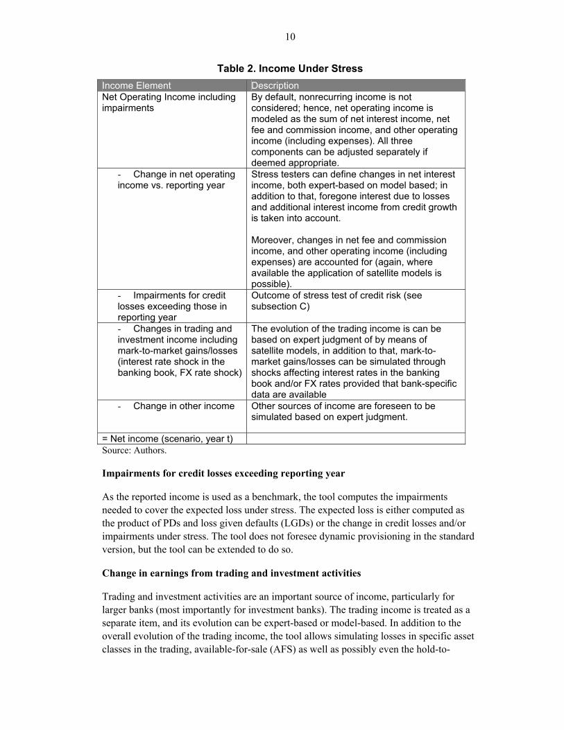
If net income becomes negative under a stress scenario, capital will take a hit, otherwise capital increases subject to taxation and the earnings retention rate. The latter is common under baseline scenarios, for example, but also in case of less severe stress scenarios. Besides the pre-shock capitalization (which is given as an input) the main drivers of solvency risk for banks are the pre-impairment operating income and the impairments themselves (provisions for credit and valuation losses of trading and investment assets, unless captured through the operating income). An overview of how the net income is handled is displayed in Table 2.
In case of using a Basel I/Basel II StA type framework, RWAs for credit risk under stress are determined by reducing the RWAs prior to stress by the exposure lost due to stress while accounting for credit growth. For IRB banks (and when using QIRB, see below), the RWAs are adjusted to reflect the change in unexpected losses, i.e., portfolio quality under stress, in addition to accounting for credit losses23 and credit growth. The framework also allows for an adjustment of RWAs for market and operational risks, and other Pillar 1 and Pillar 2 risks under stress.
B. Income
Besides an adequate level of capitalization, income is banks’ first line of defense against (unforeseen) losses. Therefore, it is a key element of any (multi-period) solvency stress testing exercise. If possible, the simulation of total income overall and/or specific components of income, respectively, should be guided by satellite models. Stress testers could use satellite models to determine (a) net interest income (or determine gross interest income and interest expenses separately); (b) net fee and commission income; (c) trading
22 In the more general, multi-period case, net profit (in each year) is added and/or subtracted from capital, subject to dividend pay-out (and the earnings retention rate, respectively) and taxation.
23 It is assumed that the RWAs for the exposure subject to credit losses is 2.5 times as high as for the total portfolio (e.g., for a bank with a risk weight of 80 percent on average, exposure subject to default is assumed to be risk-weighted at 200 percent prior to default) which has been determined based on expert judgment. Stress testers should cross-check whether this assumption applies in the situation at hand and modify the figure, if applicable.
9
income;24 and (d) other income sources (e.g., non-operating income). Interest income is usually the most important source of income, and is thus the most important one to be modeled separately.
In the standard version of the tool, post-shock income is determined as shown in Table 2. The reported operating income net of impairments serves as a benchmark for the income of the following years.25 The guiding idea is that non-recurring income as well as other sources of income are not taken into account, as these elements are not an integral part of the (medium-term) earning capacity of banks.26 The calculation of income strikes a balance between setting straightforward assumptions and more sophisticated modeling.
If the resulting net income after stress is positive, then the portion foreseen to be retained (after tax) based on the stress test assumptions will be added to the capital, otherwise losses will be deducted from capital. Rather than sticking to a general assumption about retained income, rules depending on the post-shock capitalization of each specific bank could be referred to (in line with Basel III maximum pay-out rules), but such rules are not part of the standard version of the tool.
Changes in net operating income
The net interest income is usually the most important source of income for banks and is therefore treated separately in the tool. Assumptions can either be expert-based or satellite model-based, taking into account the situation at hand. Other income elements affecting net interest income (particularly interest expenses, such as funding costs) can be added to this key position, including through satellite models. It is important to avoid double-counting in this context, which remains subject to the discretion of the stress tester.
The net fee and commission is less important that the net interest income for most banks, but is nevertheless one of the core sources of income of banks in general (particularly investment banks). Moreover, given the low interest environment during recent years, banks have shifted their reliance on interest income to other sources of income, particularly fee and commission income. Hence, it is also treated separately in the tool. Assumptions can either be expert-based or satellite model-based, taking into account the situation at hand. Other operating income is not foreseen to be modelled separately, and assumptions are foreseen to be made jointly with other income.
24 In specific cases, other components of income could also be modeled. Moreover, the link between the trading income and macroeconomic conditions is often weak, pragmatic assumptions (based on expert judgment) could be used instead.
25 If a stress test should be based on a different initial value (e.g., net interest income as the average ratio of net interest income over total loans to customers over the last x years), minor adaptations in the Excel links of the framework are necessary.
26 Stress testers should alter this assumptions is deemed appropriate under specific conditions.
10
Table 2. Income Under Stress
Income Element Description Net Operating Income including impairments
By default, nonrecurring income is not considered; hence, net operating income is modeled as the sum of net interest income, net fee and commission income, and other operating income (including expenses). All three components can be adjusted separately if deemed appropriate.
- Change in net operating income vs. reporting year
Stress testers can define changes in net interest income, both expert-based on model based; in addition to that, foregone interest due to losses and additional interest income from credit growth is taken into account. Moreover, changes in net fee and commission income, and other operating income (including expenses) are accounted for (again, where available the application of satellite models is possible).
- Impairments for credit losses exceeding those in reporting year
Outcome of stress test of credit risk (see subsection C)
- Changes in trading and investment income including mark-to-market gains/losses (interest rate shock in the banking book, FX rate shock)
The evolution of the trading income is can be based on expert judgment of by means of satellite models, in addition to that, mark-to-market gains/losses can be simulated through shocks affecting interest rates in the banking book and/or FX rates provided that bank-specific data are available
- Change in other income Other sources of income are foreseen to be simulated based on expert judgment.
= Net income (scenario, year t) Source: Authors.
Impairments for credit losses exceeding reporting year
As the reported income is used as a benchmark, the tool computes the impairments needed to cover the expected loss under stress. The expected loss is either computed as the product of PDs and loss given defaults (LGDs) or the change in credit losses and/or impairments under stress. The tool does not foresee dynamic provisioning in the standard version, but the tool can be extended to do so.
Change in earnings from trading and investment activities
Trading and investment activities are an important source of income, particularly for larger banks (most importantly for investment banks). The trading income is treated as a separate item, and its evolution can be expert-based or model-based. In addition to the overall evolution of the trading income, the tool allows simulating losses in specific asset classes in the trading, available-for-sale (AFS) as well as possibly even the hold-to-
11
maturity portfolios (HTM). The tools simulate mark-to-market gains and/or losses of specific asset classes (such as sovereign debt holdings, for example) and/or from market conditions (changes of interest rates, foreign exchange rates27), which are then accounted for through the P&L.28 It is important to avoid double-counting.
Change in other income
Other sources of income, such as other non-operating income are foreseen to be simulated based on expert judgment. The tool foresees that other operating income is also part of the same assumption. Nonrecurring income is omitted (by default), so stress testers can change the setting if deemed necessary under specific circumstances.
C. Credit Losses
The simulation of credit risk under stress is the key innovation of the tool. The treatment of credit risk is based on a Basel II/III type notion. Accordingly, the simulation of credit risk is based on the credit risk parameters used for the computation of IRB capital charges, namely PDs, LGD ratios, Exposures at Default (EADs), and maturities and asset correlations. The tool offers a conceptual framework to determine credit losses under stress on the hand one (which inform the numerator of capital adequacy) and RWAs for credit risk under stress on the other (the denominator of key capitalization ratios), which is further outlined below. It is worth highlighting that credit risk analyses are assumed to be carried out for all assets subject to default risk, i.e., including counterparty credit risk. The market risk of the liquid assets is simulated separately through income. The relationship between PDs and LGDs
During the last decade, there has been an intense debate on the empirical relationship between PDs and LGDs. It has been proposed that there should be a positive relationship between PDs and LGDs because the stresses that cause PDs to increase would also make defaults more severe or would reduce the value of collateral. For bonds, a positive correlation has been found early on (Altman et al. 2003, for example), which implies that in times of stress (i.e., higher PDs), LGDs are also higher than in ‘normal’ times. With more data becoming available during the last years for loans, it has been confirmed that this relationship does also hold true for loans (see Moody’s 2009 and S&P 2010, for example; Appendix III).
In order to provide stress testers with the possibility to link stressed LGDs to stressed PDs (and thus avoiding the need to make a separate assumption about the development of
27 The impact of interest rate shocks on banks’ P&L is assumed to be done outside the tool. The tool allows simulating (linear) variations of the shocks. Foreign exchange rate shocks are simulated based on net open positions.
28 The authors are aware that some portfolio gains/losses are not accounted in the P&L but directly against capital, however, there is no economic, only an accounting difference, which for tractability reasons has not been included in the framework.
12
LGDs under stress) we combine evidence determined by Moody’s (2009) with an approximation formula proposed by the U.S. Federal Reserve (2006) to determine downturn LGDs, i.e., LGDs under stress conditions.29 Using the formula by the Fed:
Downturn-LGD = 0.08 + 0.92*Long-term average30 LGD (2)
an adjusted linear formula (2) is derived, accounting for the finding that the relationship between PDs and LGDs is non-linear (S&P 2010,31 for example).32
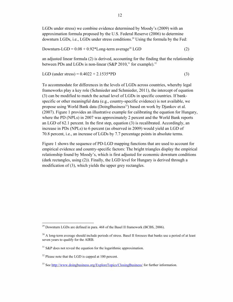
LGD (under stress) = 0.4022 + 2.1535*PD (3) To accommodate for differences in the levels of LGDs across countries, whereby legal frameworks play a key role (Schmieder and Schmieder, 2011), the intercept of equation (3) can be modified to match the actual level of LGDs in specific countries. If bank-specific or other meaningful data (e.g., country-specific evidence) is not available, we propose using World Bank data (DoingBusiness33) based on work by Djankov et al. (2007). Figure 1 provides an illustrative example for calibrating the equation for Hungary, where the PD (NPLs) in 2007 was approximately 2 percent and the World Bank reports an LGD of 62.1 percent. In the first step, equation (3) is recalibrated. Accordingly, an increase in PDs (NPLs) to 6 percent (as observed in 2009) would yield an LGD of 70.8 percent, i.e., an increase of LGDs by 7.7 percentage points in absolute terms.
Figure 1 shows the sequence of PD-LGD mapping functions that are used to account for empirical evidence and country-specific factors: The bright triangles display the empirical relationship found by Moody’s, which is first adjusted for economic downturn conditions (dark rectangles, using (2)). Finally, the LGD level for Hungary is derived through a modification of (3), which yields the upper grey rectangles.
29 Downturn LGDs are defined in para. 468 of the Basel II framework (BCBS, 2006).
30 A long-term average should include periods of stress. Basel II foresees that banks use a period of at least seven years to qualify for the AIRB.
31 S&P does not reveal the equation for the logarithmic approximation.
32 Please note that the LGD is capped at 100 percent.
33 See http://www.doingbusiness.org/ExploreTopics/ClosingBusiness/ for further information.
13
Figure 1. Link Between LGD and PD, Illustrative Example for Hungary
Source: Authors.
D. Risk-Weighted Assets
To compute RWAs for credit risk in economic terms (both to determine the level and to compute changes under stress), one needs a portfolio credit risk model. The tool uses the one-factor-model underlying the IRB approach to determine changes of RWAs conditional on changes in credit risk parameters (PDs, correlations, and name concentration). The level of RWAs used for the computation can be chosen as follows: (a) using economic RWAs (IRB, economic capital requirements); (b) using QIRB-adjusted Basel I/StA RWAs (scaling factor, see below); (c) using RWAs based on Basel I/StA. LGDs exhibit a linear relationship with RWAs, so there is no need to establish a model. PDs and RWAs Stress conditions in credit risk affect banks’ solvency (i.e., capital ratios) in two different ways (a) an increase in expected losses (ELs), not covered by pricing or provisions, can hit capital should net income become negative; (b) an increase in the riskiness of the performing loans portfolio (unexpected losses) leads to a raise of RWAs. While the calculation of ELs is straightforward (as the effect is linear), the calculation of RWAs is not (as the effect is non-linear due to correlations).
14
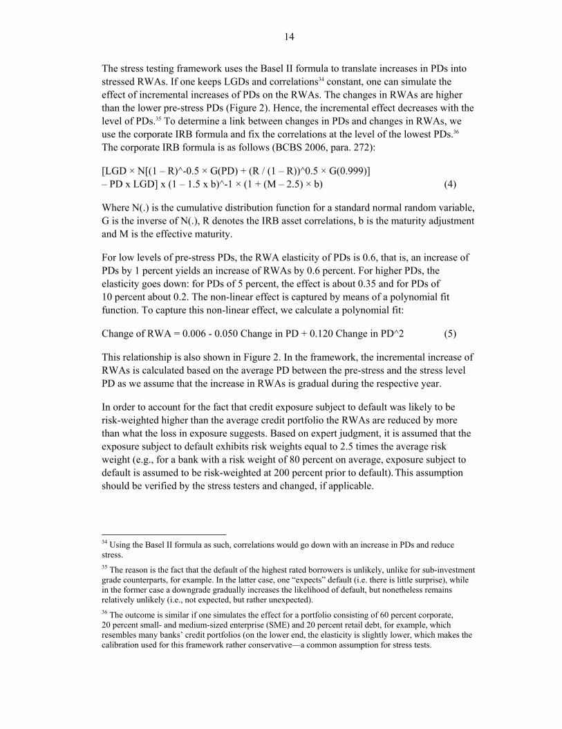
The stress testing framework uses the Basel II formula to translate increases in PDs into stressed RWAs. If one keeps LGDs and correlations34 constant, one can simulate the effect of incremental increases of PDs on the RWAs. The changes in RWAs are higher than the lower pre-stress PDs (Figure 2). Hence, the incremental effect decreases with the level of PDs.35 To determine a link between changes in PDs and changes in RWAs, we use the corporate IRB formula and fix the correlations at the level of the lowest PDs.36 The corporate IRB formula is as follows (BCBS 2006, para. 272):
[LGD × N[(1 – R)^-0.5 × G(PD) + (R / (1 – R))^0.5 × G(0.999)] – PD x LGD] x (1 – 1.5 x b)^-1 × (1 + (M – 2.5) × b) (4)
Where N(.) is the cumulative distribution function for a standard normal random variable, G is the inverse of N(.), R denotes the IRB asset correlations, b is the maturity adjustment and M is the effective maturity.
For low levels of pre-stress PDs, the RWA elasticity of PDs is 0.6, that is, an increase of PDs by 1 percent yields an increase of RWAs by 0.6 percent. For higher PDs, the elasticity goes down: for PDs of 5 percent, the effect is about 0.35 and for PDs of 10 percent about 0.2. The non-linear effect is captured by means of a polynomial fit function. To capture this non-linear effect, we calculate a polynomial fit:
Change of RWA = 0.006 - 0.050 Change in PD + 0.120 Change in PD^2 (5)
This relationship is also shown in Figure 2. In the framework, the incremental increase of RWAs is calculated based on the average PD between the pre-stress and the stress level PD as we assume that the increase in RWAs is gradual during the respective year.
In order to account for the fact that credit exposure subject to default was likely to be risk-weighted higher than the average credit portfolio the RWAs are reduced by more than what the loss in exposure suggests. Based on expert judgment, it is assumed that the exposure subject to default exhibits risk weights equal to 2.5 times the average risk weight (e.g., for a bank with a risk weight of 80 percent on average, exposure subject to default is assumed to be risk-weighted at 200 percent prior to default). This assumption should be verified by the stress testers and changed, if applicable.
34 Using the Basel II formula as such, correlations would go down with an increase in PDs and reduce stress. 35 The reason is the fact that the default of the highest rated borrowers is unlikely, unlike for sub-investment grade counterparts, for example. In the latter case, one “expects” default (i.e. there is little surprise), while in the former case a downgrade gradually increases the likelihood of default, but nonetheless remains relatively unlikely (i.e., not expected, but rather unexpected). 36 The outcome is similar if one simulates the effect for a portfolio consisting of 60 percent corporate, 20 percent small- and medium-sized enterprise (SME) and 20 percent retail debt, for example, which resembles many banks’ credit portfolios (on the lower end, the elasticity is slightly lower, which makes the calibration used for this framework rather conservative—a common assumption for stress tests.
15
Figure 2. Incremental Impact of an Increase of PDs on RWAs
0.0%
0.1%
0.2%
0.3%
0.4%
0.5%
0.6%
0.7%
0% 5% 10% 15% 20%
Incremental Impact on RWAs per 1% change of PD(PD on the x-axis, Impact on the y-axis)
Incremental Impact Poly. (Incremental Impact) Source: Authors’ Calculations based on Basel II IRB formula.
Asset correlations and RWAs In a similar vein, we assess the RWA elasticity of asset correlations, i.e., the impact of an increase of asset correlations on RWAs while holding PDs and LGDs constant. As shown in Table 3, the impact based on the IRB formula (4) depends on the asset class and the pre-stress level of PDs. For the corporate IRB formula, for example, the effect is more than linear (i.e., the PD elasticity is above 1) for PDs lower than 2 percent. As a robustness check,37 we compare the previous results with empirical evidence provided by Mager and Schmieder (2009). Based on stress tests of synthetic, but realistic German credit portfolios, the authors find that the RWA elasticity for small banks is 0.45, for medium-sized banks 0.7 and for large German banks 1.25, which confirms the previous parameters. As a default setting, the framework is based on a linear relationship between asset correlations and RWAs, but stress testers can modify this assumption. In sum, the framework allows to provide similar functionalities of an economic capital model (such as CreditMetrics, CreditRisk+) by reduced form models. Together with the possibility to include capital charges for name concentration (Section III.D.d) the framework approximates a fully-fledged credit portfolio model.
37 This is also to account for the fact that the correlations in the IRB framework have been modeled conditional on the PD.
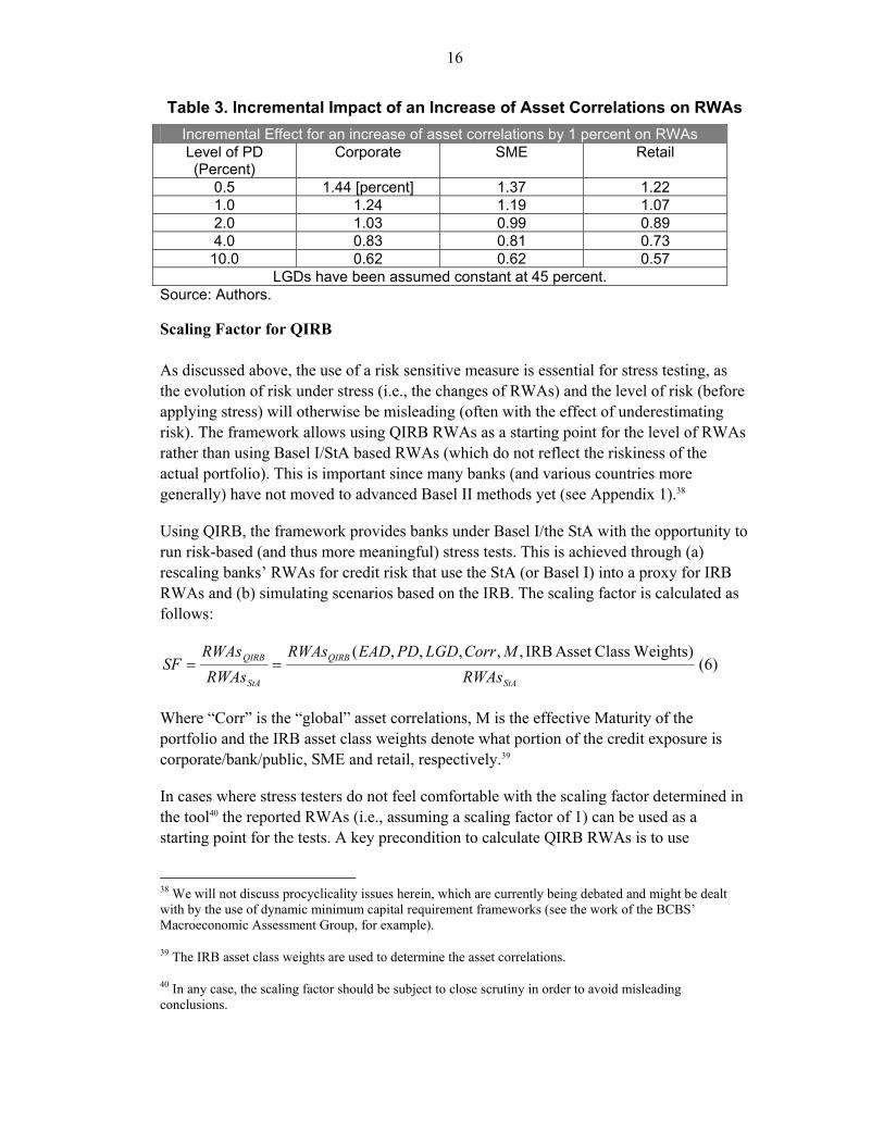
16
Table 3. Incremental Impact of an Increase of Asset Correlations on RWAs
Incremental Effect for an increase of asset correlations by 1 percent on RWAs Level of PD (Percent)
Corporate SME Retail
0.5 1.44 [percent] 1.37 1.22 1.0 1.24 1.19 1.07 2.0 1.03 0.99 0.89 4.0 0.83 0.81 0.73
10.0 0.62 0.62 0.57 LGDs have been assumed constant at 45 percent.
Source: Authors.
Scaling Factor for QIRB As discussed above, the use of a risk sensitive measure is essential for stress testing, as the evolution of risk under stress (i.e., the changes of RWAs) and the level of risk (before applying stress) will otherwise be misleading (often with the effect of underestimating risk). The framework allows using QIRB RWAs as a starting point for the level of RWAs rather than using Basel I/StA based RWAs (which do not reflect the riskiness of the actual portfolio). This is important since many banks (and various countries more generally) have not moved to advanced Basel II methods yet (see Appendix 1).38
Using QIRB, the framework provides banks under Basel I/the StA with the opportunity to run risk-based (and thus more meaningful) stress tests. This is achieved through (a) rescaling banks’ RWAs for credit risk that use the StA (or Basel I) into a proxy for IRB RWAs and (b) simulating scenarios based on the IRB. The scaling factor is calculated as follows:
StA
QIRB
StA
QIRB
RWAs
MCorrLGDPDEADRWAs
RWAs
RWAsSF
) WeightsClassAsset IRB,,,,,( (6)
Where “Corr” is the “global” asset correlations, M is the effective Maturity of the portfolio and the IRB asset class weights denote what portion of the credit exposure is corporate/bank/public, SME and retail, respectively.39
In cases where stress testers do not feel comfortable with the scaling factor determined in the tool40 the reported RWAs (i.e., assuming a scaling factor of 1) can be used as a starting point for the tests. A key precondition to calculate QIRB RWAs is to use
38 We will not discuss procyclicality issues herein, which are currently being debated and might be dealt with by the use of dynamic minimum capital requirement frameworks (see the work of the BCBS’ Macroeconomic Assessment Group, for example).
39 The IRB asset class weights are used to determine the asset correlations.
40 In any case, the scaling factor should be subject to close scrutiny in order to avoid misleading conclusions.
17
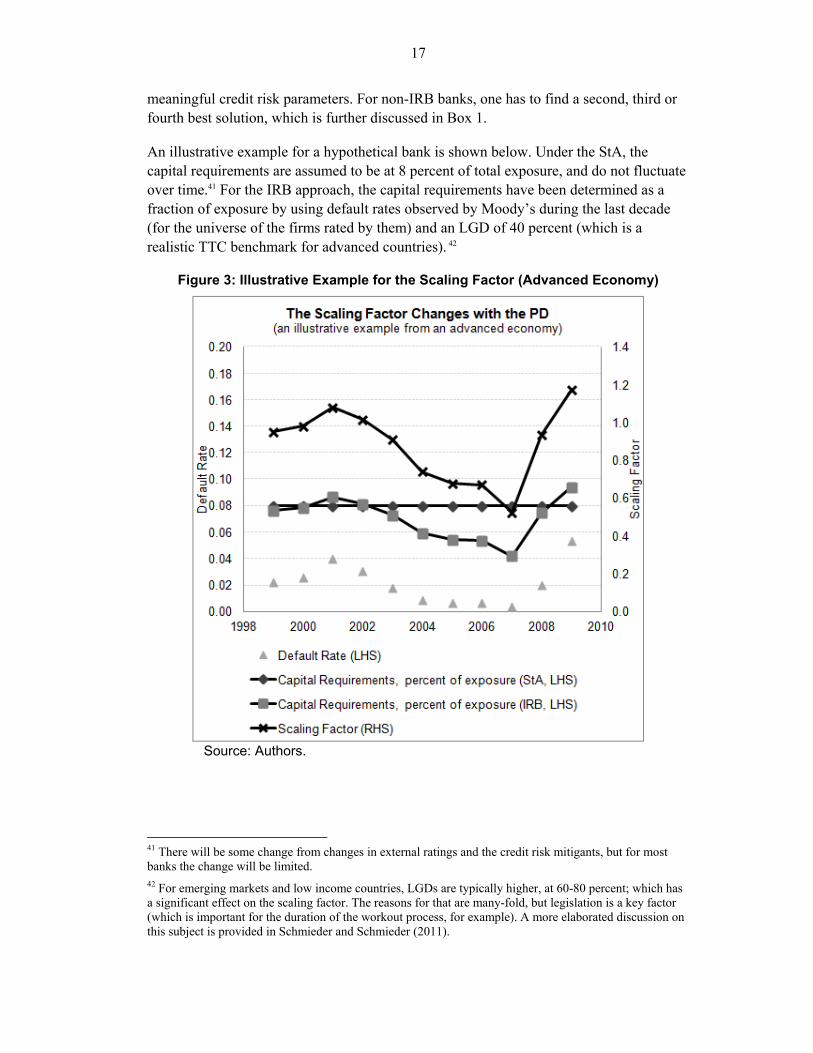
meaningful credit risk parameters. For non-IRB banks, one has to find a second, third or fourth best solution, which is further discussed in Box 1.
An illustrative example for a hypothetical bank is shown below. Under the StA, the capital requirements are assumed to be at 8 percent of total exposure, and do not fluctuate over time.41 For the IRB approach, the capital requirements have been determined as a fraction of exposure by using default rates observed by Moody’s during the last decade (for the universe of the firms rated by them) and an LGD of 40 percent (which is a realistic TTC benchmark for advanced countries). 42
Figure 3: Illustrative Example for the Scaling Factor (Advanced Economy)
Source: Authors.
41 There will be some change from changes in external ratings and the credit risk mitigants, but for most banks the change will be limited. 42 For emerging markets and low income countries, LGDs are typically higher, at 60-80 percent; which has a significant effect on the scaling factor. The reasons for that are many-fold, but legislation is a key factor (which is important for the duration of the workout process, for example). A more elaborated discussion on this subject is provided in Schmieder and Schmieder (2011).
18
In the example, the capital requirements under the IRB fluctuate significantly over time and are lower during most years (e.g., during 2003 to 2008).43 The scaling factor (crosses, Right-hand scale), compares the relative level of capital requirements between the StA and the IRB approach over time. The scaling factor thus adjusts the level of the StA RWA to the level of the IRB capital requirements.
Due to the high level of LGDs for most emerging markets and low income countries, the scaling factor would be above 1 except for very benign years with very low PDs, indicating that economic risk is often underestimated by the StA capital ratio, which thereby might give a false sense of security (see also Hardy and Schmieder, 2011).
Name Concentration and RWAs Basel II IRB minimum capital requirements do not account for name concentration, as they are based on the assumption that portfolios are perfectly granular. While this assumption helps keeping the underlying model (the one-factor-model) relatively simple, capital requirements may therefore be underestimated. In order to avoid such underestimation—which is likely to be the case for small banks—concentration risk is subject to Pillar 2, i.e., supervisory scrutiny. We refer to a study by Gordy and Luetkebomert (2007), who came out with a framework to estimate name concentration.
The outcome of a numerical example provided by Gordy and Luetkebohmert was used by the authors to determine an approximation formula that translates name concentration into additional RWAs (in percent). This approximation depends on the actual level of name concentration as measured in terms of the Herfindahl-Hirschman-Index (HHI44) and the aggregate bank-level PD.
0.1))*1)-PD/0.4%((1*HHI)*599.120.02(*100RWA (7)
Gordy and Luetkebomert (2007) found if the HHI of a portfolio is 0.01, for example, the Pillar 2 capital requirements’ add-on for name concentration risk (the so-called granularity adjustment) is about 15 percent of RWAs for credit risk, all else being equal. If one also accounts for changes of PDs from the level that has been used for calibration, i.e., 0.4 percent, to for example 0.8 percent, then the Pillar II add-on would be 16.5 percent. The granularity adjustment increases by 10 percent in relative terms for an increase of PDs by 0.4 percentage points, in line with the findings by the authors. To illustrate the impact of name concentration on RWAs we use data for synthetic but realistic credit portfolios of German banks as reported by Mager and Schmieder (2009). 43 The reason for this observation is the fact that the Basel II framework has been calibrated with a view that IRB capital charges are, on average, lower than the ones under StA (in the primary recipient countries, i.e. not the ones that voluntarily adopt Basel II), reflecting economic reasons on the one hand and proving banks with incentives to move to the IRB on the other.
44 The HHI is the sum of the squared exposure portions. Gordy and Luetkebomert refer to an HHI calculated based on exposures for groups/borrower units.
19
Accordingly, for a portfolio of a small bank (assuming that the HHI45 is about 0.02 and an average PD of 2 percent), the granularity adjustment is 40 percent, for a medium-sized bank (HHI: 0.005; PD: 1.2 percent) 10 percent and for a large bank (HHI: 0.0006; PD: 0.8 ercent) about 3 percent.
To ensure that the applied method is consistent with the sample used for calibration, the definition of borrower units has to be compared with the one underlying the calibration sample46. If the definition for the stress test sample is less conservative, then name concentration is likely to be underestimated, otherwise the opposite is true.
E. Basel III
In order to simulate the phase-in of Basel III rules (see Figure 5 for an overview), the tool allows making a broad assessment of the potential impact over time, informed by the outcome of the QIS 6 (BCBS 2010b). More specific assumptions can be added provided that bank-specific data is available. The simulation includes three key elements (see BCBS 2010a): (i) An increase of RWAs. (ii) The phase-out of eligible capital from 2013 (Total Capital, Tier 1) and 2014
(Common/Core Tier 1), respectively. (iii) Changes in the minimum capital ratios over time.
Changes in the first two elements are simulated based on the outcome of the QIS 6, and applied to banks according to their size (banks with equity less than USD 3 billion are classified as Group 2 banks).
For the increase in RWAs, stress testers can define a portion of behavioral adjustment. If one assumes that there is a behavioral adjustment by 50 percent, for example, then banks are assumed to mitigate 50 percent of the expected increase of RWAs—through a change of their asset structure, for example. Together with the finding that RWAs for Group 1 banks increase by 23 percent, on average, the increase in RWAs become 11.5 percent. For Group 2 banks, the increase is 50 percent of 4 percent, i.e., 2 percent.
According to the QIS 6, the phase-out of capital eligibility (for core tier 1 capital called “phase-in of capital deductions) for Tier 1 capital amounts to 30.2 percent (Group 2 banks: 14.1 percent) and for total capital to 26.8 percent (16.6 percent). As foreseen by the Basel III schedule, the tool simulated a gradual phase-out by 10 percent of the current
45 The HHI is a commonly used measure to determine concentration. It denotes the sum of the squared portfolio contribution of each element (here: each credit to the total credit exposure of a bank).
46 The definition of connected borrowers is based on the German banking act (“KWG”), para. 19 (2) (see http://www.iuscomp.org/gla/statutes/KWG.htm#19). A more comprehensive definition of borrower units (or “group of connected clients”, respectively), which could serve as a benchmark, has been proposed by the predecessor to the European Banking Authority, CEBS.
20
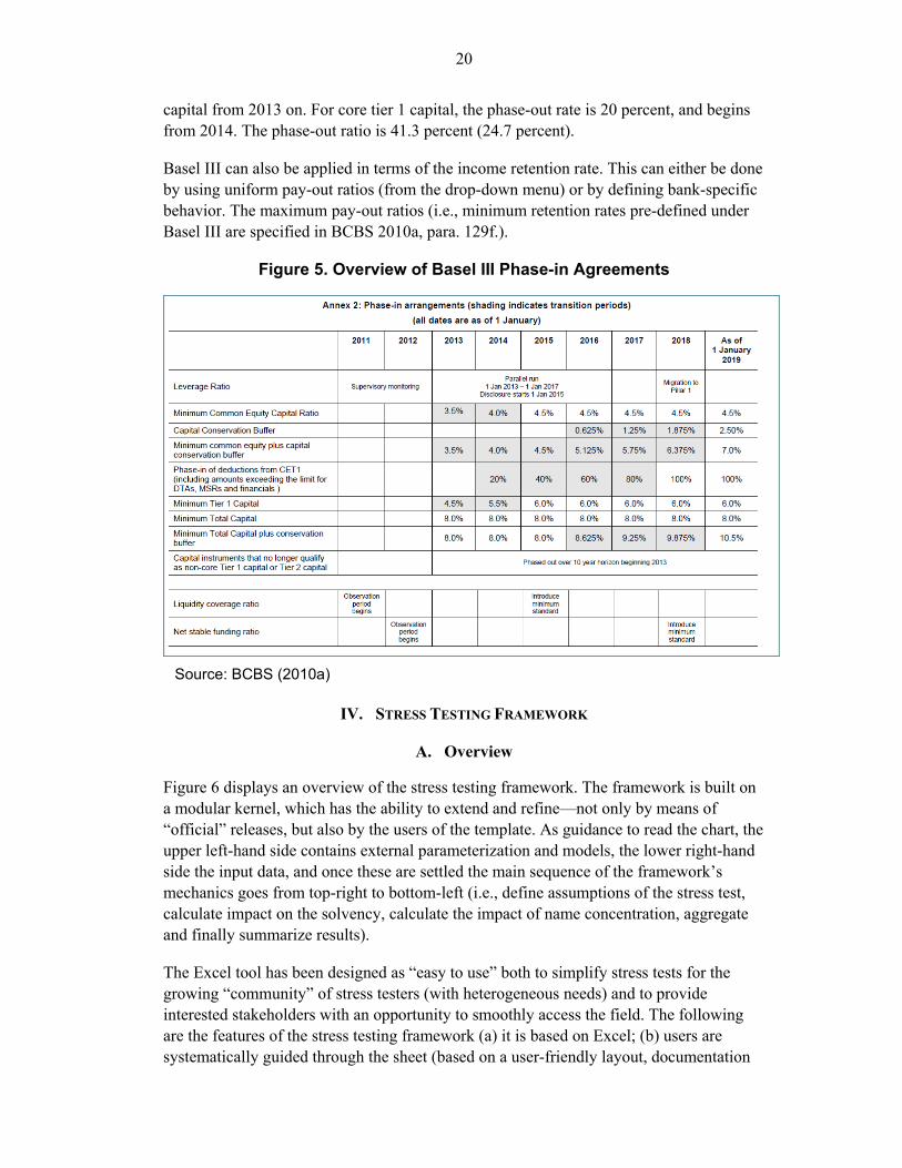
capital from 2013 on. For core tier 1 capital, the phase-out rate is 20 percent, and begins from 2014. The phase-out ratio is 41.3 percent (24.7 percent).
Basel III can also be applied in terms of the income retention rate. This can either be done by using uniform pay-out ratios (from the drop-down menu) or by defining bank-specific behavior. The maximum pay-out ratios (i.e., minimum retention rates pre-defined under Basel III are specified in BCBS 2010a, para. 129f.).
Figure 5. Overview of Basel III Phase-in Agreements
Source: BCBS (2010a)
IV. STRESS TESTING FRAMEWORK
A. Overview
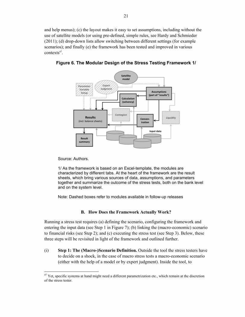
Figure 6 displays an overview of the stress testing framework. The framework is built on a modular kernel, which has the ability to extend and refine—not only by means of “official” releases, but also by the users of the template. As guidance to read the chart, the upper left-hand side contains external parameterization and models, the lower right-hand side the input data, and once these are settled the main sequence of the framework’s mechanics goes from top-right to bottom-left (i.e., define assumptions of the stress test, calculate impact on the solvency, calculate the impact of name concentration, aggregate and finally summarize results).
The Excel tool has been designed as “easy to use” both to simplify stress tests for the growing “community” of stress testers (with heterogeneous needs) and to provide interested stakeholders with an opportunity to smoothly access the field. The following are the features of the stress testing framework (a) it is based on Excel; (b) users are systematically guided through the sheet (based on a user-friendly layout, documentation
21
and help menus); (c) the layout makes it easy to set assumptions, including without the use of satellite models (or using pre-defined, simple rules, see Hardy and Schmieder (2011); (d) drop-down lists allow switching between different settings (for example scenarios); and finally (e) the framework has been tested and improved in various contexts47.
Figure 6. The Modular Design of the Stress Testing Framework 1/
Concen-tration
ParameterVariable
Setup
Liquidity
ExpertJudgment
Input data
Satellite model
Assumptions(part of “results”)
Resultsummary
Results(incl. balance sheets)
Calculation(solvency)
Contagion
Concen-tration
ParameterVariable
Setup
Liquidity
ExpertJudgment
Input data
Satellite model
Assumptions(part of “results”)
Resultsummary
Results(incl. balance sheets)
Calculation(solvency)
Contagion
Source: Authors.
1/ As the framework is based on an Excel-template, the modules are characterized by different tabs. At the heart of the framework are the result sheets, which bring various sources of data, assumptions, and parameters together and summarize the outcome of the stress tests, both on the bank level and on the system level.
Note: Dashed boxes refer to modules available in follow-up releases
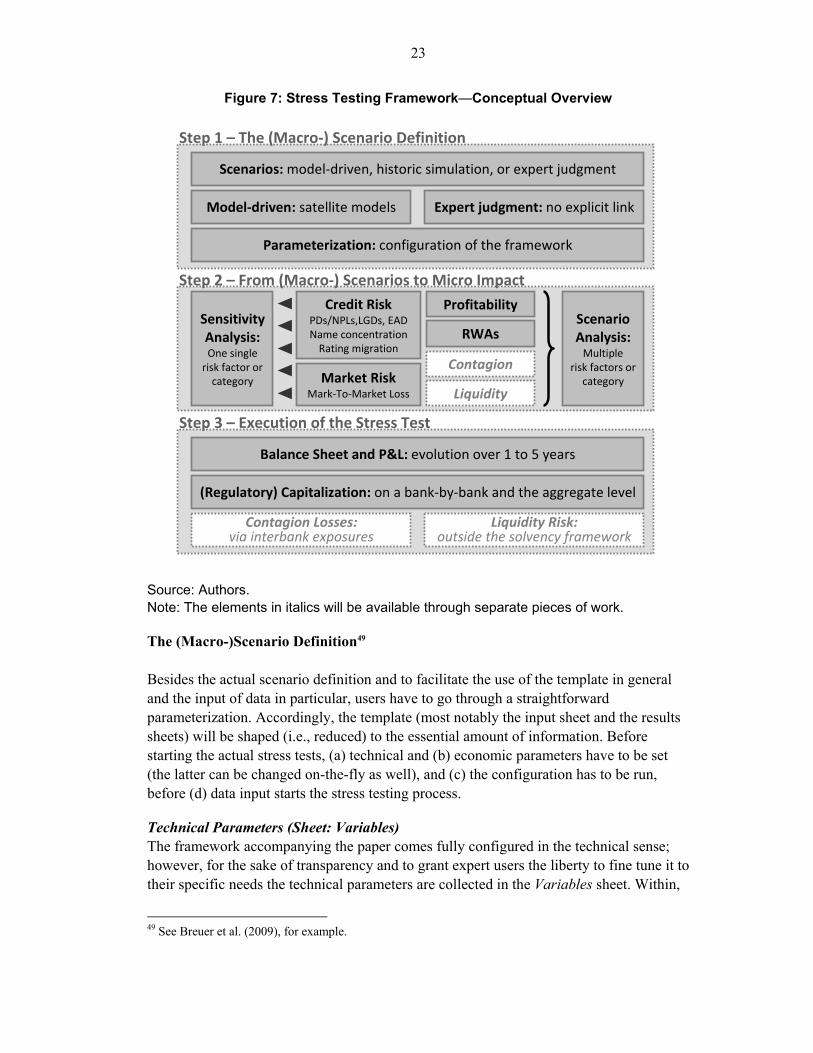
B. How Does the Framework Actually Work?
Running a stress test requires (a) defining the scenario, configuring the framework and entering the input data (see Step 1 in Figure 7); (b) linking the (macro-economic) scenario to financial risks (see Step 2); and (c) executing the stress test (see Step 3). Below, these three steps will be revisited in light of the framework and outlined further. (i) Step 1: The (Macro-)Scenario Definition. Outside the tool the stress testers have
to decide on a shock, in the case of macro stress tests a macro-economic scenario (either with the help of a model or by expert judgment). Inside the tool, to
47 Yet, specific systems at hand might need a different parametrization etc., which remain at the discretion of the stress tester.
22
facilitate the use of the template in general and the input of data in particular, users first have to go through a straightforward parameterization that alters the template according to the number of banks, and the (credit) portfolio granularity, for example.48
It is highly advisable to run reverse stress tests (i.e., to test banks’ thresholds to cope with stress) in addition to scenario tests. Reverse tests should include simulations of uniform scenarios (e.g., simulating how banks can cope with a stress level of, say 3 percent) as scenarios that simulate stress based on current figures (i.e., losses during the last period) tend to “punish” banks that experienced high losses while other banks might be treated too favorably (this is not the case if stress testers work with forward-looking PDs).
(ii) Step 2: From (Macro-)Scenarios to Micro Impact. In the simplest case, stress testers run sensitivity tests for specific risk types, such as credit, market, operational, or concentration risks. In the more demanding case, including when an assessment is linked-to a macroeconomic scenario (referred to as macro stress test) multiple risk factors are accounted for at the same time. In the latter case, the impact of the stress test is performed by linking (macro-economic) risk factors to financial risks (i.e., banks’ asset quality) by means of so-called satellite models (i.e., econometric models).
(iii) Step 3: The execution of the stress tests. The actual run of the tests happens “on the fly” i.e., once the specific setting has been chosen, and the satellite models calibrated, the final outcome in terms of banks’ balance sheets and capitalization is immediately shown. For the solvency tests, the tests reveal bank-by-bank solvency under stress and aggregate figures for the system (for example, capital adequacy and recapitalization needs) as well as various financial soundness indicators (FSIs), including the risk contributions of different elements (operating income serving as a first buffer against losses, credit losses, and trading and investment losses) to stress.
48 This step can be omitted, which means that some redundant information is displayed, but otherwise (and more generally) all functionality will be available. More generally, a general purpose was to ensure that technical constraints (e.g., with the included macros; using a previous Excel version) do not result in limitations to apply the framework as such.
23
Figure 7: Stress Testing Framework—Conceptual Overview
Credit RiskPDs/NPLs,LGDs, EADName concentration
Rating migration
Scenarios: model-driven, historic simulation, or expert judgment
Step 1 – The (Macro-) Scenario Definition
Step 2 – From (Macro-) Scenarios to Micro Impact
Step 3 – Execution of the Stress Test
Parameterization: configuration of the framework
Model-driven: satellite models Expert judgment: no explicit link
SensitivityAnalysis:One single
risk factor orcategory Market Risk
Mark-To-Market Loss
Profitability
RWAs
Contagion
Liquidity
ScenarioAnalysis:
Multiplerisk factors or
category
Balance Sheet and P&L: evolution over 1 to 5 years
(Regulatory) Capitalization: on a bank-by-bank and the aggregate level
Contagion Losses: via interbank exposures
Liquidity Risk:outside the solvency framework
Source: Authors. Note: The elements in italics will be available through separate pieces of work.
The (Macro-)Scenario Definition49 Besides the actual scenario definition and to facilitate the use of the template in general and the input of data in particular, users have to go through a straightforward parameterization. Accordingly, the template (most notably the input sheet and the results sheets) will be shaped (i.e., reduced) to the essential amount of information. Before starting the actual stress tests, (a) technical and (b) economic parameters have to be set (the latter can be changed on-the-fly as well), and (c) the configuration has to be run, before (d) data input starts the stress testing process.
Technical Parameters (Sheet: Variables) The framework accompanying the paper comes fully configured in the technical sense; however, for the sake of transparency and to grant expert users the liberty to fine tune it to their specific needs the technical parameters are collected in the Variables sheet. Within,
49 See Breuer et al. (2009), for example.
24
a wide variety of fundamental parameters can be changed: from banking aggregates and available Basel II approaches, via scenario and Visual Basic (VB) variable names to the configuration of VB look-up tables. Although the technical parameters should come as a great advantage to tailor the tool to the needs of expert users, novices (a) do not have to care about them; and (b) should familiarize themselves with the tool prior to changing entries, as the knock-on effects are potentially vast. Economic Parameters (Sheet: Parameter) Also in terms of economic parameterization, the accompanying framework is fully configured. At the same time the sheet Parameter allows the stress tester to reconfigure according to individual needs. 50 This includes amongst others the under-year adjustment (in case of non-year-end flow data), scenario labels, and interest rate shocks, but also all reduced form approximations that define the relationship among different risk factors, including the change of RWAs ((i)–(iii) and their level pre stress (iv)):
i. The relationship between PDs and LGDs. ii. The relationship between PDs and RWAs.
iii. The relationship between Asset Correlations and RWAs. iv. The rescaling of credit-risk related RWAs based on StA into QIRB RWAs.
For a detailed explanation of each of these relationships, please refer to either the Parameter tab in the tool or Section III. Configuration (Sheet: Setup)
Finally, the last configuration is the only parameterization step every user of the framework has to go through. In comparison to the other two, it is a straight forward configuration of a number of basic parameters in the Setup sheet of the tool, where the scope of a stress test is defined. The framework accounts for (a) the number of banks included in the test; (b) the choice of credit portfolio granularity—at the moment either by economic sector, Basel II asset class or by geography (regions within a country and/or other countries/world regions banks lent to)51; and (c) the general granularity of data available for the tests (there is a choice between a minimum set of data, an extended set and a maximum set). Accordingly, the templates will be tailored displaying only relevant information, which is done by means of VB macros. The procedure to do so is explained in detail within the tool.
50 The vast majority of this economic parameterization is pre-defined, but stress testers are expected to verify the information and change, if applicable.
51 Either of the breakdowns (sector and/or geography) can be adjusted as part of the parameterization as well.
25
Input Data (Sheet: Input_X52)
Running stress tests requires various inputs, comprising a set of system-level data (such as the GDP for the system, as well as country-level PDs53 and LGDs), bank-specific information (balance sheet data, other financial statements and regulatory data) as well as econometric models, if applicable.
The amount of inputs needed to run stress tests determines the methods that can be used. For the most relevant set of data and bank-specific information, the framework offers three different sets of input data. At a minimum, about 30 inputs are needed to run a solvency test, which includes the bank names, the reporting year and month and the country of origin, for example. Using the minimum set of data comes at the costs of the lowest precision of the results,54 but most functionalities of the tool are available also in the case of using minimum input data.55
The extended set of bank-level data includes bank-specific credit risk parameters (EADs, PDs, and LGDs) for (key) economic sectors, which allows for more accurate results and additional tests. In order to keep the inputs limited, one can refer to broad sectors, for example corporate, retail, public and financials.56 The maximum set of information comprises about 600 inputs and is meant to provide a meaningful stress test for a first tier international bank, good enough to serve for instance as a top-down (TD) benchmark for the SCAP or EBA exercises. It is also key highlighting that one can run tests for a sample of banks where a different set of information is available; for example, the extended or maximum set of information could be available for some banks (the larger ones), and the minimum for other (smaller) banks and the tool will use the most useful (i.e., granular information) for each of the banks. It is important to verify whether the “intelligence” built into the tool in that respect is adequate for the situation at hand.
Publicly available data (for example annual reports, risk reports and, ideally, Basel Pillar 3 reports) allows running tests based on the minimum and extended set, in some cases also for the maximum set. Hence, the tool can also be used by stakeholders outside the supervisory community. A natural question is how to run economically meaningful tests
52 Where “_X” stands for either: Banks, Country or Satellite.
53 In the simplest case, non-performing loans (NPLs) (i.e., the stock) can be used as a proxy for PDs.
54 It is foreseen that credit risk parameters (NPLs or provisions) are available at the bank level. If this is not the case, country-level parameters can be used as a proxy.
55 In order to verify this statement, the outcome of a solvency stress test for the same bank using minimum, extended and maximum information has been compared.
56 Again, parameters such as the LGDs can be based on country-level data or expert judgment.
26
for banks that have not (yet) implemented advanced Basel II approaches. The solution is to use proxies, as further outlined in Box 1.
From (Macro-)Scenarios to Micro Impact
The framework has been developed with a view to providing the users with some guidance for the definition of the stress tests. Besides the (technical) parameterization and the scope in terms of data, this feature is mostly related to the assumptions that define the stress tests. It is, however, important to note that this guidance is meant as a general benchmark, but does not substitute the final judgment of the person running the tests, which is essential to account for the idiosyncrasies of specific countries and/or banks. In the simplest case, stress testers run sensitivity stress tests for specific risk types, such as credit, market, operational, or concentration risks. Although not exclusively the case, most sensitivity stress tests are based on expert judgment. The stress tester specifies the increase of the risk parameters based on judgment, for example by referring to stress levels observed in the past. This is a rather straightforward procedure, guided (a) by the available risk factors (for example using regulatory or economic capital requirements, see below); and (b) defining the scope of the stress tests, i.e., which assets the stress is referred to.
In the more complex case, scenario stress tests are run. These are multivariate stress tests mostly based on a simulation of stressed macro conditions (hence labeled macro stress tests), but can be based on expert judgment as well. In the former case, a stress test is performed by linking (or “translating”) macro-economic forecasts to financial risks (i.e., banks’ asset quality), by means of satellite models. The pertinent satellite models are not part of the framework accompanying the paper and will therefore not be discussed in detail.
However, the framework provides a “user exit” on a predefined tab Input_Satellite that allows the specification of linking models for PDs, credit growth and changes in profitability. Although these linking equations have to be estimated outside the framework, the framework itself allows including up to five different explanatory variables per equation (which can be extended easily). Moreover, Input_Satellite allows for up to four different scenarios (baseline and three stress scenarios) that can be conveniently chosen and changed on the results sheet to allow for sensitivity analysis around the central macro-economic scenario. Information on the handling of satellite models in the tool is provided in Appendix II as well as in the roadmap in the tool, including how to specify additional models, including on a bank level.
27
Box 1. How to do a Meaningful Stress Test as a non-IRB Bank? A key precondition to run economic stress tests is how to use meaningful credit risk parameters. The natural (first best) solution is to use credit parameters (PDs, LGDs) estimated by banks as part of their IRB analysis. The key advantage of PDs is that they are forward-looking, whereby banks which recently faced (or recognized) high losses are not necessarily the ones that are likely to “expect” comparably high losses in the future. However, such data is often not available, so one has to find a second or third best solution. In most countries, non-performing loans (NPLs) are available, usually including time series. However, NPLs are often stock figures and definitions vary widely across countries; hence, a feasible solution has to be found to determine PD-like figures. A second best solution is (a) using available NPL inflows or (b) translating NPL stocks into flows based on expert judgment (while ensuring that the resulting proxies are consistent with default rates); another second best option (c), benefitting from the fact that such data is often readily available is using flow data of credit impairments from the P&L (or specific provisions and/or write-offs). Inflows of losses directly measure credit losses, whereby PDs and LGDs do not have to be determined separately. Otherwise, losses can be decomposed into default rates and LGDs, respectively. A third best solution is using NPL stocks. Ultimately, country-specific data or data from peer countries can be used as a proxy (fourth best solution). LGDs are often available on a country-level only. If bank-specific data is not available, ideally on a sectoral level (first best solution) country-specific data is a meaningful proxy, particularly for corporate exposure (the Doing Business database by World Bank contains data for most countries). For other sectors, for example retail exposure, an alternative proxy could be defined, reflecting higher or lower recovery rates. It is important to notice that Basel II parameters (notably the ones for the FIRB) have been calibrated for advanced countries, where LGD levels are usually substantially lower than in emerging economies and low income countries. To run economic stress tests, the StA based capital ratios of banks have to be translated into economic capital ratios. This is done by calculating quasi-IRB RWAs (for credit risk) based on implied credit risk parameters (PDs and LGDs or credit losses). Economically meaningful RWAs for market risk can be derived from internal experience (or other benchmark data), while RWAs for operational risk could be based on statutory data. The translation for credit risk could be done based on the sector composition of the credit portfolio of each bank. The total RWA is then calculated as the sum of the RWAs for the different asset classes, using the respective Basel II IRB formula (SMEs, retail credit, and other types of counterparts). Depending on the level of the implied credit risk parameters, i.e. the TTC level in a specific country as well as the state of the cycle, the economic capital ratio is lower or higher than under statutory rules (i.e., StA capital rules). The relative difference is captured by a scaling factor. In addition to that, a surcharge for name concentration can be calculated, and added to the RWAs computed beforehand. The rationale for this so-called granularity adjustment is that the Basel IRB framework assumes that there is no name concentration, whereby the capital ratio particularly for medium-sized and smaller banks (which exhibit smaller and thus more concentration portfolios) is too low. It is important to compare the definition of borrower units against the definition used to calibrate the formula (see main text). A conservative benchmark is the EU definition of related counterparties.
28
Assumptions (Sheet: Assumptions)
The scenarios are selected on the results sheets, which allow direct access to the results, i.e., the stress tester does not have to change tabs. Accordingly, a series of stress tests can conveniently be run, i.e., the sensitivity of the results to various parameters and settings assessed. The stress tester may want to simulate capitalization under stress in case of an ad-hoc increase of NPLs or of PDs by 50 percent or 100 percent in relative terms, for example an increase from 1 percent to 2 percent (increase by 100 percent).57If the stress tester seeks to run more fine-tuned scenarios, including bank-specific scenarios, they have to be entered on the assumptions sheet.
In order to run a comprehensive scenario test, assumptions have to be made for nine stress test parameters as displayed in Table 4. While the stress level for the RWAs for market risk and operational risk has to be defined based on expert judgment (e.g., referring to the experience of specific banks or specific countries), the framework allows determining RWAs based on the credit risk parameters, depending on the setting (StA or IRB) and based on the parameterization (as pre-defined on the Parameter tab, see also previous section). Moreover, to ease the use of macro stress tests, simplified models to link changes in macroeconomic conditions (reflected in changes of GDP) to credit risk parameters and income have been predefined for advanced countries and emerging economies on the tab Parameter.58 If the stress tester chooses the option to empirically link the LGDs to the PDs, only stressed PDs have to defined, while the level of the LGDs will be derived based on an empirical model (also found on the tab Parameter).
57 Stress levels can be defined either in absolute (“to x percent”) or in relative terms (“by x percent”) without entering scenarios manually.
58 These simplified rules (“rules of thumb”) are based on forthcoming research by Hardy and Schmieder (2011). However, stress testers should be careful not to overly rely on the rules as they are meant to depict “average” situations only rather than to capture country-specific circumstances.

29
Table 4. Assumptions for Risk Parameters Parameter Description Credit Risk (CR) PDs Change in Ratings
Set bank-level and/or sector-specific PDs. PDs can, in principle, be proxied by NPLs, taking into account the country- and/or bank-specific circumstances. Used to simulate a change of ratings by up t 9 notches.59
LGD Credit Losses
(PD*LGD)
Set bank-level and/or sector-specific LGDs. Using credit losses (e.g., provisions) as a proxy for PDs and LGDs. Credit losses could again be based on bank-level data or determined by sector.
Asset Correlations (ACs)
Largest Exposures
Set the stress level of asset correlations. Used to simulate default of largest counterparts.
Credit Growth Define growth of total credit exposure. Market Risk (MR) FX Rate, Interest
Rate, Asset Prices Set stress levels for foreign exchange (FX) rates, interest rates and asset prices.
Change in RWAs Set stress levels for RWAs. Operational Risk (OR) Set the increase in RWAs for operational risk. Pillar 2 RWAs Set the increase in RWAs for Pillar 2 exposure (and
other Pillar 1 risks). Change in Income Set changes operating income (net interest income,
fee and commission income, other operating income) and other income (other non-operating income).60
Basel III Simulation of the potential impact of Basel III, namely (a) the increase in RWAs (according to QIS 6 results); (b) the phase-out of capital (according to QIS 6 results); and (c) the minimum capitalization rates as scheduled (for Total Capital, Tier 1 capital and Common/Core Tier 1)
Source: Authors.
Other assumptions allowing for tailor-made stress tests are summarized in Table 5. These assumptions include (a) choosing a scenario as such; (b) running tests based on different sector classifications, for example industry sectors and regions; (c) choosing a method how to stress RWAs for credit risk; (d) choosing whether to include name concentration
59 This test is only available if one enters the maximum set of data.
60 Double-counting with shocks to market risk factors has to be avoided.
30
risk; and (v) defining bank behavior under stress and (6) setting the hurdle rates for difference capital ratios.
Table 5. Other Assumptions
Scenario Description Type of scenario The user can simulate a macro scenario,61 an
expert based scenario, and a scenario based on manual input.
Sector classification If data for different sectors have been entered, then one has to choose the sector classification to be used for the tests.
Method to stress RWAs for credit risk
RWAs for credit risk can be stressed based on a StA type method (essentially by keeping RWAs constant) or by means of the Basel II IRB approach. In the latter case, banks are more sensitive to changes in credit risk parameters, particularly if pre-stress levels of losses are low (due to the non-linearity of the Basel II IRB model). In case banks are using the StA, a stress tester can use a scaling factor to translate the pre-stress RWAs into QIRB (i.e., economic) RWAs. However, if doing so, the stress tester has to verify whether the scaling factor is appropriate.
Name concentration The stress tester can add RWAs for name concentration to the RWAs reported by a bank, which can then be further stressed.
Bank behavior Income retention rate Change of balance sheet
The stress tester has to define the level of income to be retained, which can have a significant effect of the results. An assumption is needed how the balance sheet changes, notably the total amount of credit exposure.
Selection of capital definition and Hurdle Rate for the tests
Depending on the availability of information, the framework allows simulating solvency tests for three different capital definitions (e.g., Total capital, Tier 1, Common Tier 1) and defining the respective hurdle rates (e.g., 8 percent) for each year.
Source: Authors.
61 Macro scenarios can be defined for various parameters. Stress testers can also choose a simplified macro model for specific parameters, which is based on changes of GDP growth only, and distinguishes between advanced countries and emerging countries. The simplified model should be used with great care and the parameters should be modified as needed.
31
The Execution of the Stress Tests A key advantage of the framework is that the actual run of the tests happens “on the fly” i.e., once the specific setting has been chosen the final outcome of the tests is shown in the respective results tabs. The tests reveal bank-by-bank solvency under stress (capital ratio and recapitalization needs, if applicable) and aggregate metrics for the system (capital adequacy, recapitalization needs) as well as various FSIs, including the risk contributions of different risk elements (credit losses, trading losses, income serving as a first buffer against losses) to stress.
Balance Sheet Mechanics
The mechanics of the spreadsheet are summarized on the road-map tab step-by-step.
Results of the Tests
The results sheets not only allow defining the methods, but also display the results of the tests, both on the level of the financial system (or the overall sample of banks) and on an institution-specific level.
In Figure 8, the dispersion of the bank-specific outcomes of a macro stress test for 12 international banks through 2014 is shown. The output shows the evolution of different quantiles of the capital ratios over time and the number of banks in different capital buffer ranges. The outcome for the system (which is not shown herein) includes the number of banks failing the tests, capitalization needs in absolute and relative terms, as well as the contribution of different risk drivers to stress.
32
Figure 8. Screenshot of Bank-Specific Results
Label Percentile 2009 2010 2011 2012 2013 2014Min 0 11.0% 6.7% 5.2% 4.3% 1.7% 0.0%Quart 25 25 13.3% 9.7% 9.8% 11.7% 10.9% 11.1%Median 50 13.9% 10.9% 11.4% 15.0% 14.1% 14.4%Quart 75 75 17.6% 12.8% 13.3% 17.5% 17.1% 18.2%Max 100 47.9% 36.6% 33.4% 39.2% 34.7% 33.2%
-99999999 <8% 0 2 2 1 2 28% <11% 0 4 4 2 1 1
11% <14% 6 3 4 3 3 314% <17% 3 2 1 2 3 217% <20% 0 0 0 3 2 220% <23% 2 0 0 0 0 123% >=23% 1 1 1 1 1 1
Total Capital Ratio Distribution of Scenario Analysis
0%
20%
40%
60%
80%
100%Distribution of Capital Ratios
-10%
0%
10%
20%
30%
40%Interquartile Capital Ratio Ranges
Source: Authors.
V. Stylized Numerical Example
The basic functioning of the tool will be illustrated based on a simplified example, namely the simulation of stress for one bank and one period with a focus on credit risk only. We take the example of a bank currently using the Basel II standardized approach with total assets of $10 billion, thereof a credit portfolio of $5.7 billion, and total regulatory capital of $1.3 billion. The bank’s expected loss amounts to $0.1 billion (EAD: 5.7 billion; PD: 2.4 percent; LGD: 71.8 percent). The total RWAs (which included market and operational risk) based on the StA are assumed to be $10 billion and the RWAs based on the QIRB are $13.4 billion (the scaling factor would hence be 1.34 for all RWAs). It is assumed that a stress tester seeks to simulate two scenarios, namely an increase of PDs by 100 percent in both cases, and an increase of LGDs (and asset correlations) by 7.2 percent (and 20 percent) for scenario 2 as shown in Table 6. In case of scenario 2, concentration risk is added to the RWAs, accounting for 4 percent of the total RWAs for credit risk.62
62 It is important to highlight that the scenarios are meant for illustration and should not be used as whatsoever k kind of benchmark scenarios (unless this is justified in the situation at hand).
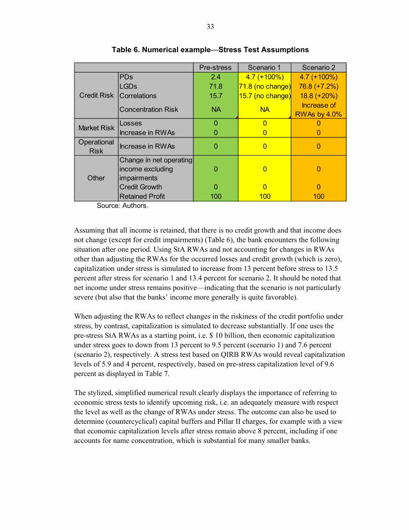
33
Table 6. Numerical example—Stress Test Assumptions
Pre-stress Scenario 1 Scenario 2PDs 2.4 4.7 (+100%) 4.7 (+100%)LGDs 71.8 71.8 (no change) 76.8 (+7.2%)Correlations 15.7 15.7 (no change) 18.8 (+20%)
Concentration Risk NA NAIncrease of
RWAs by 4.0%Losses 0 0 0Increase in RWAs 0 0 0
Operational Risk
Increase in RWAs 0 0 0
Change in net operating income excluding impairments
0 0 0
Credit Growth 0 0 0Retained Profit 100 100 100
Credit Risk
Market Risk
Other
Source: Authors.
Assuming that all income is retained, that there is no credit growth and that income does not change (except for credit impairments) (Table 6), the bank encounters the following situation after one period. Using StA RWAs and not accounting for changes in RWAs other than adjusting the RWAs for the occurred losses and credit growth (which is zero), capitalization under stress is simulated to increase from 13 percent before stress to 13.5 percent after stress for scenario 1 and 13.4 percent for scenario 2. It should be noted that net income under stress remains positive—indicating that the scenario is not particularly severe (but also that the banks’ income more generally is quite favorable). When adjusting the RWAs to reflect changes in the riskiness of the credit portfolio under stress, by contrast, capitalization is simulated to decrease substantially. If one uses the pre-stress StA RWAs as a starting point, i.e. $ 10 billion, then economic capitalization under stress goes to down from 13 percent to 9.5 percent (scenario 1) and 7.6 percent (scenario 2), respectively. A stress test based on QIRB RWAs would reveal capitalization levels of 5.9 and 4 percent, respectively, based on pre-stress capitalization level of 9.6 percent as displayed in Table 7. The stylized, simplified numerical result clearly displays the importance of referring to economic stress tests to identify upcoming risk, i.e. an adequately measure with respect the level as well as the change of RWAs under stress. The outcome can also be used to determine (countercyclical) capital buffers and Pillar II charges, for example with a view that economic capitalization levels after stress remain above 8 percent, including if one accounts for name concentration, which is substantial for many smaller banks.
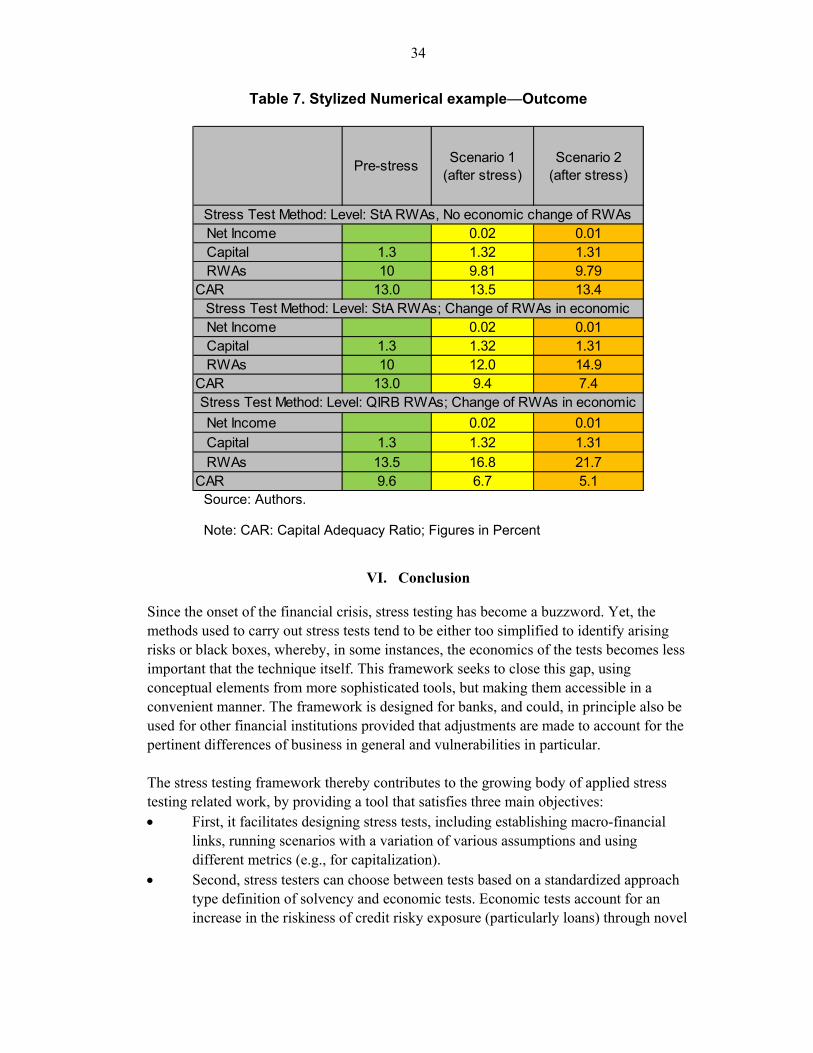
34
Table 7. Stylized Numerical example—Outcome
Pre-stressScenario 1
(after stress)Scenario 2
(after stress)
Net Income 0.02 0.01 Capital 1.3 1.32 1.31 RWAs 10 9.81 9.79CAR 13.0 13.5 13.4
Net Income 0.02 0.01 Capital 1.3 1.32 1.31 RWAs 10 12.0 14.9CAR 13.0 9.4 7.4
Net Income 0.02 0.01
Capital 1.3 1.32 1.31
RWAs 13.5 16.8 21.7CAR 9.6 6.7 5.1
Stress Test Method: Level: StA RWAs; Change of RWAs in economic
Stress Test Method: Level: QIRB RWAs; Change of RWAs in economic
Stress Test Method: Level: StA RWAs, No economic change of RWAs
Source: Authors.
Note: CAR: Capital Adequacy Ratio; Figures in Percent
VI. Conclusion
Since the onset of the financial crisis, stress testing has become a buzzword. Yet, the methods used to carry out stress tests tend to be either too simplified to identify arising risks or black boxes, whereby, in some instances, the economics of the tests becomes less important that the technique itself. This framework seeks to close this gap, using conceptual elements from more sophisticated tools, but making them accessible in a convenient manner. The framework is designed for banks, and could, in principle also be used for other financial institutions provided that adjustments are made to account for the pertinent differences of business in general and vulnerabilities in particular. The stress testing framework thereby contributes to the growing body of applied stress testing related work, by providing a tool that satisfies three main objectives: First, it facilitates designing stress tests, including establishing macro-financial
links, running scenarios with a variation of various assumptions and using different metrics (e.g., for capitalization).
Second, stress testers can choose between tests based on a standardized approach type definition of solvency and economic tests. Economic tests account for an increase in the riskiness of credit risky exposure (particularly loans) through novel
35
approaches to approximate risk-weighted assets under stress, including for banks who have not adopted advanced Basel II approaches.
Third and finally, the ease of use (and communication) of stress testing tools (results) by providing a tractable Excel-based framework that yields accessible results for decision makers (for example, policy makers and senior bank managers) and/or market participants.
To that end, the framework provides a generic balance sheet tool around which various building blocks are centered that increase the risk-sensitivity of stress tests. Likewise, the framework allows stress testers running a series of tests for a number of different risk factors within a short period of time in order to get a comprehensive view of potential vulnerabilities of a bank and/or banking system. Moreover, the framework is flexible for various amendments—as it is Excel based—catering to the need of stress testers. Such amendments have been added to the tool for instance during stress testing exercises in the course of recent (European) FSAPs and at the ECB. At the same time, it is important to highlight that the ultimate economics to run meaningful stress tests remain the primary responsibility of the stress tester. It is up to the stress tester to decide how financial risks of specific banks link to macroeconomic stress, for example, but also how plausible (i.e., likely) specific scenarios are given the situation at hand. An important pre-condition to run more meaningful stress tests (particularly in emerging economies and low income countries) is to improve data, which is particularly the case for the area of credit risk. The latter will gradually allow using forward-looking credit parameters (PDs), which will make the calculations more reliable. It will avoid “punishing” banks that exhibited high losses in the reporting (for example those that “cleaned” their portfolios), as such a loss level could be carried forward if tests are backward-looking. Meaningful data will also reveal economic risks that remain otherwise hidden, which is true for the LGDs in emerging economies and low income countries as well as name concentration risk (in smaller banks). In emerging markets, running economic tests is highly crucial to reveal true risk levels—not least to avoid a false sense of security. As such the stress testing framework accompanying the paper is a work in progress. In further releases, modules aimed at liquidity and contagion risk will be made available. Moreover, the tool will be expanded to account for ongoing regulatory changes, evolution of best practice, for example the definition of scenarios.
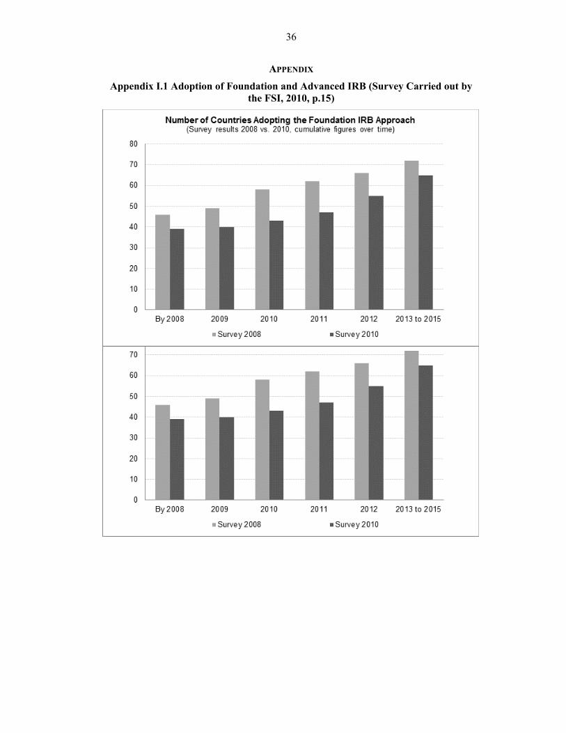
36
APPENDIX
Appendix I.1 Adoption of Foundation and Advanced IRB (Survey Carried out by the FSI, 2010, p.15)
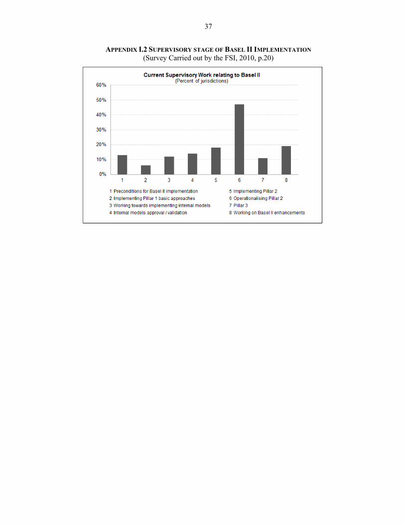
37
APPENDIX I.2 SUPERVISORY STAGE OF BASEL II IMPLEMENTATION (Survey Carried out by the FSI, 2010, p.20)
�

38
APPENDIX II. DERIVATION OF MACRO SCENARIOS
The macro scenarios are derived based on satellite models, i.e., econometric models linking macroeconomic variables to financial risk parameters. The framework foresees that such models are calibrated before running the tests, and that the outcome of the regressions is entered into a specifically foreseen tab. The advantage is that assumptions entered in the template can be changed readily and one can assess the sensitivity of the stress test outcome to changes in the macroeconomic assumptions. The framework foresees the definition of three macro scenarios, namely mild stress (yellow, macro 1), stress of medium severity (orange, macro 2) and severe stress (red, macro 3). Once the model specification has been entered into the “Satellite Model” tab, the credit parameter scenarios are directly linked to the respective column in the assumptions tab. The framework contains illustrative models that link macroeconomic conditions to PDs/Default Rates/NPLs, credit growth and income. Stress testers are cautioned not the use these models unless there is a reason to believe that they are suitable for the circumstances of their test.
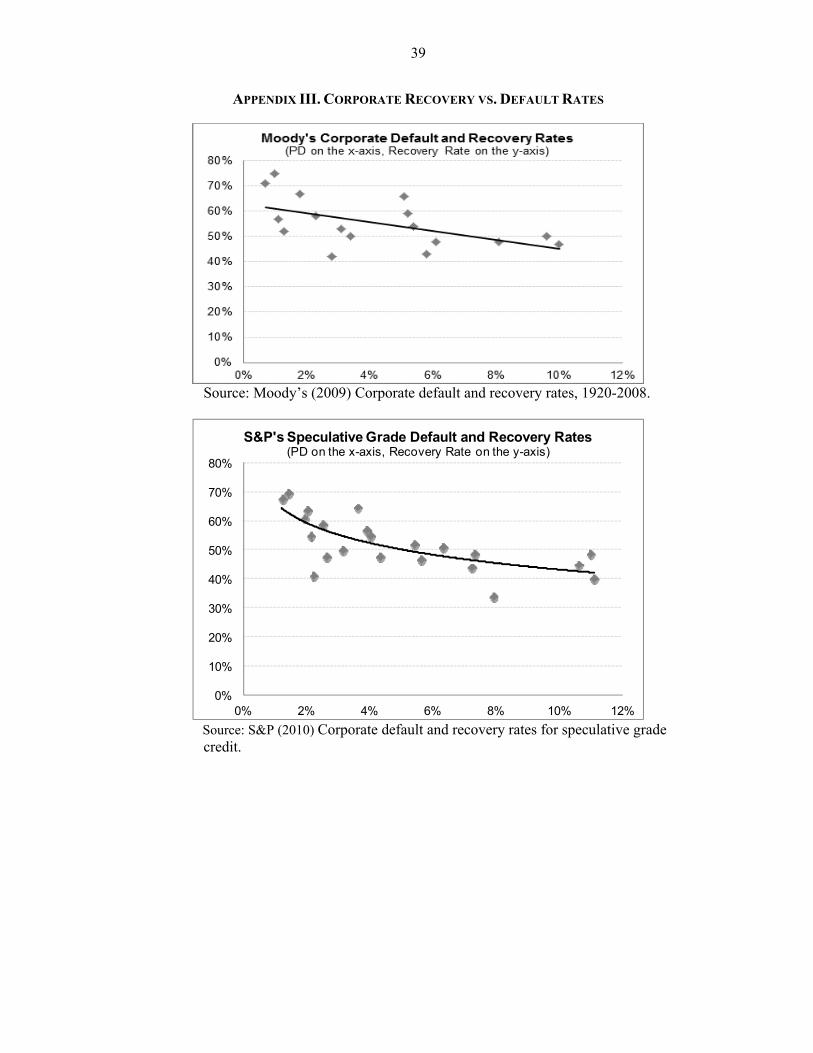
39
APPENDIX III. CORPORATE RECOVERY VS. DEFAULT RATES
Source: Moody’s (2009) Corporate default and recovery rates, 1920-2008.
0%
10%
20%
30%
40%
50%
60%
70%
80%
0% 2% 4% 6% 8% 10% 12%
S&P's Speculative Grade Default and Recovery Rates(PD on the x-axis, Recovery Rate on the y-axis)
Source: S&P (2010) Corporate default and recovery rates for speculative grade credit.
40
REFERENCES Aikman, David, and others, 2009, “Funding liquidity risk in a quantitative model of systemic stability,” Bank of England, Working Paper No. 372. Altman, Edward I., Brooks Brady, Andrea Resti, and Andrea Sironi, “The Link Between Default and Recovery Rates: Theory, Empirical Evidence and Implications,” NYU Working Paper No. S-DRP-03-08, March. Alessandri, Piergiorgio, and others, 2009, “Towards a Framework for Quantifying Systemic Stability,” International Journal of Central Banking 5, pp. 47-82. Alfaro, Rodrigo A., and Mathias Drehmann, 2009, “Macro Stress Tests and Crises: What Can We Learn,” BIS Quarterly Review December. Basel Committee on Banking Supervision (BCBS), 2006, “Basel II: International
Convergence of Capital Measurement and Capital Standards: A Revised Framework–Comprehensive Version”, June. http://www.bis.org/publ/bcbs128.htm.
Basel Committee on Banking Supervision (BCBS), 2010a, “Basel III: A Global Regulatory Framework for More Resilient Banks and Banking System,” December. Basel Committee on Banking Supervision (BCBS), 2010b, “Results of the Comprehensive Quantitative Impact Study,” December. Breuer,Thomas, Martin Jandacka, Klaus Rheinberger, and Martin Summer, 2009, “How to Find Plausible, Severe, and Useful. Stress Scenarios,” International Journal of Central Banking 5, 205-224. Borio, Claudio, and Mathias Drehmann, 2009, “Towards an Operational Framework for Financial Stability: ‘Fuzzy’ Measurement and its Consequences,” in Banco Central de Chile (ed), Financial Stability, Monetary Policy and Central Banking: also available as BIS Working Paper no. 284. Boss, Michael, Gerald Krenn, Claus Puhr, and Martin Summer, 2006, “Systematic Risk Monitor: A Model for Systematic Risk Analysis and Stress Testing of Banking Systems,” Austrian National Bank, Financial Stability Report 11. Boss, Michael, and others, 2008, “Stress Tests for the Austrian FSAP Update 2007: Methodology, Scenarios and Results,” Austrian National Bank, Financial Stability Report 15. Čihák, Martin, 2007, “Introduction to Applied Stress Testing,” IMF Working Paper 07/59 (Washington: International Monetary Fund). Djankov, Simeon, Caralee McLiesh, and Andrei Shleifer, 2007, “Private Credit in 129 Countries,” Journal of Financial Economics 84, pp. 299–329.
41
Drehmann, Mathias, Steffen Sorensen, and Marco Stringa, 2008, “The Integrated Impact of Credit and Interest Rate Risk on Banks: An Economic Value and Capital Adequacy Perspective,” Bank of England Working Paper No. 339. Eisenberg, Larry K. and Thomas H. Noe, 2001, “Systemic Risk in Financial Systems,”
Management Science, Vol. 47(2): pp. 236–249. Elsinger, Helmut, Alfred Lehar, and Martin Summer, 2006, “Risk Assessment for Banking Systems,” Management Science, Vol. 52(9), pp. 1,301–1,314. Federal Reserve Board of Governors, 2007, “Draft Federal Register Notice,” p. 119. Financial Stability Institute, 2010, “2010 FSI Survey on the Implementation of the New Capital Adequacy Framework—Summary of Responses to the Basel II Implementation Survey,” Occasional Paper No 9, August. Foglia, Antonella, 2008, “Stress Testing Credit Risk: A Survey of Authorities' Approaches,” Banca d’Italia, Occasional Papers no. 37, December. Goodhart, Charles A.E., Pojanart Sunirand, and Dimitrios P. Tsomocos, 2003, “A Model to Analyze Financial Fragility,” London School of Economics, Discussion Paper 417. Gordy, Michael and Eva Lütkebohmert, 2007, “Granularity Adjustment for Basel II.” Deutsche Bundesbank Discussion Paper (Series 2), No 1, 2007. Gray, Dale F., Zvi Bodie, and Robert C. Merton, 2007, “New Framework for Measuring and Managing Macrofinancial Risk and Financial Stability,” NBER Working Paper No. 13607 Hardy, Daniel, and Christian Schmieder, “Rules of Thumb to Stress Test Credit Risk,” Forthcoming IMF Working Paper. Mager, Ferdinand, and Christian Schmieder, 2009, “Stress Testing German Credit Portfolios,” Journal of Risk Model Validation 3(3), pp. 61-77. Moody’s, 2009, “Corporate Default and Recovery Rates”, 1920-2008, Special Comment, February. Schmieder, Christian, and others, 2011, “Second Generation Applied Stress Testing— Liquidity Module,” Forthcoming IMF Working Paper. Schmieder, Christian and Philipp Schmieder, 2011, Impact of Legislation on Credit Risk—Comparative Evidence From the United States, the United Kingdom, and Germany, “IMF Working Paper 11/55 (Washington: International Monetary Fund). Schuermann, Til, 2004, “What Do We Know About Loss Given Default?” Working Paper 04-01, Wharton Financial Institutions Center Working Paper Series, www.defaultrisk.com/pp_recov_40.htm.
42
Standard & Poor’s, 2010, “Default, Transition, and Recovery: 2009 Annual Global Corporate Default Study and Rating Transitions”.