Bachelor Thesis

in Computer Science

Next-Generation Feature Modelswith Pseudo-Boolean SAT Solvers

Sebastian Henneberg

Advisor:

Dr.-Ing. Sven Apel

October 28, 2011

Abstract

Feature models are an important artifact in software product lineengineering. They describe commonality and variability of allproduct line members. This thesis proposes the use of attributesand additional constraints in feature modeling to extend expres-siveness and usability. Therefore, new grammars were built toextend traditional feature models by optional integer attributesand additional constraints. We found a mapping that converts ex-tended feature models into pseudo-boolean satisfiability (PBSAT)instances. This allows reasoning of feature models using a PBSATsolver. We took different feature model analysis operations fromseveral authors to show applicability of the PBSAT representation.This required adaptations and led to extensions of known algo-rithms. We analyzed the scalability of our proposed adaptationsby an evaluation of different real-world feature models.

Contents

1 Introduction 7

2 Background 102.1 Feature models . . . . . . . . . . . . . . . . . . . . . . . . . . . . . . . 102.2 SAT and PBSAT . . . . . . . . . . . . . . . . . . . . . . . . . . . . . . . 112.3 Automated analysis . . . . . . . . . . . . . . . . . . . . . . . . . . . . . 142.4 FeatureIDE . . . . . . . . . . . . . . . . . . . . . . . . . . . . . . . . . . 15

3 Extended feature models 173.1 Attribute grammar . . . . . . . . . . . . . . . . . . . . . . . . . . . . . 173.2 Constraint grammar . . . . . . . . . . . . . . . . . . . . . . . . . . . . 183.3 Generated parser . . . . . . . . . . . . . . . . . . . . . . . . . . . . . . 19

4 Mapping feature models to logic 214.1 Feature diagram . . . . . . . . . . . . . . . . . . . . . . . . . . . . . . . 214.2 Cross-tree constraints . . . . . . . . . . . . . . . . . . . . . . . . . . . . 224.3 Additional pseudo-boolean equations and inequalities . . . . . . . . 23

5 Analysis operations 265.1 Domain engineering . . . . . . . . . . . . . . . . . . . . . . . . . . . . 26

5.1.1 Validation . . . . . . . . . . . . . . . . . . . . . . . . . . . . . . 275.1.2 Feature properties . . . . . . . . . . . . . . . . . . . . . . . . . 285.1.3 Simplification . . . . . . . . . . . . . . . . . . . . . . . . . . . . 335.1.4 Edits . . . . . . . . . . . . . . . . . . . . . . . . . . . . . . . . . 36

5.2 Application engineering . . . . . . . . . . . . . . . . . . . . . . . . . . 405.2.1 Propagation of selections . . . . . . . . . . . . . . . . . . . . . 40

6 Evaluation 446.1 Runtime behaviour . . . . . . . . . . . . . . . . . . . . . . . . . . . . . 456.2 Simplification potential . . . . . . . . . . . . . . . . . . . . . . . . . . . 45

3

6.3 Pre-processing impact . . . . . . . . . . . . . . . . . . . . . . . . . . . 46

7 Conclusion 487.1 Contributions . . . . . . . . . . . . . . . . . . . . . . . . . . . . . . . . 497.2 Further work . . . . . . . . . . . . . . . . . . . . . . . . . . . . . . . . . 49

Bibliography 51

4

List of Figures

2.1 Feature model of a mobile phone product line . . . . . . . . . . . . . 102.2 Steps of automated resasoning . . . . . . . . . . . . . . . . . . . . . . 142.3 Screenshot of the feature modeling view in FeatureIDE . . . . . . . . 15

3.1 Grammar of the attribute file . . . . . . . . . . . . . . . . . . . . . . . 183.2 Sample attribute file . . . . . . . . . . . . . . . . . . . . . . . . . . . . 183.3 Grammar of the constraint file . . . . . . . . . . . . . . . . . . . . . . . 193.4 Sample constraint file . . . . . . . . . . . . . . . . . . . . . . . . . . . . 193.5 Alternative representation of sample constraint file . . . . . . . . . . 19

4.1 Subtree of a feature diagram . . . . . . . . . . . . . . . . . . . . . . . . 234.2 Sample attribute file according to 4.1 . . . . . . . . . . . . . . . . . . . 23

5.1 A valid and a void feature model . . . . . . . . . . . . . . . . . . . . . . . 275.2 A feature model that contains features with different properties . . . 285.3 A feature model with emphasised core features . . . . . . . . . . . . . 295.4 A feature model with emphasised dead features . . . . . . . . . . . . . 305.5 A feature model with emphasised variant features . . . . . . . . . . . . 315.6 A feature model with emphasised false optional features . . . . . . . . . 325.7 Simplification of a feature model with atomic sets . . . . . . . . . . . . . 335.8 A feature model edit that is classified as generalization . . . . . . . . . . 365.9 Types of edits based on set inclusions or rather logical implications . 375.10 A user selection leads to a propagation . . . . . . . . . . . . . . . . . . . 435.11 The propagation of 5.10 represented as graph . . . . . . . . . . . . . . 43

5

List of Tables

2.2 Feature diagram mappings to propositional logic . . . . . . . . . . . . 12

4.2 Feature diagram mappings to PBSAT . . . . . . . . . . . . . . . . . . . 244.3 Additional constraint mapping according to 4.1 and 4.2 . . . . . . . . 25

5.2 The four different types of BCP clauses . . . . . . . . . . . . . . . . . . 415.4 The four different types of BCP inequalities . . . . . . . . . . . . . . . 42

6.1 Mean runtime of validation, property computation and propagation 456.2 Results of the simplification (atomic set) computation . . . . . . . . . 466.3 Mean runtime of the simplification (atomic set) algorithm . . . . . . . 47

List of Algorithms

1 Check validity of feature model . . . . . . . . . . . . . . . . . . . . . . 282 Compute set of core features . . . . . . . . . . . . . . . . . . . . . . . . 293 Compute set of dead features . . . . . . . . . . . . . . . . . . . . . . . 304 Compute set of variant features . . . . . . . . . . . . . . . . . . . . . . 315 Compute set of false-optional features . . . . . . . . . . . . . . . . . . 336 Compute the atomic sets . . . . . . . . . . . . . . . . . . . . . . . . . . 35

6

1 Introduction

Software product lines are a recent research topic in software engineering. It is aboutproducing a set of related software with similar core functionality but different pe-culiarity. Product lines are widely known from big manufacturer’s of cars and com-puters or even fast-food restaurants. They all have in common that they offer acollection of related products which satisfy different customer needs. Product linesoften enable customers to individualize products.

Apart from the advantage of smaller portfolios, product lines reduce costs and helpto unify the development process. Especially larger software systems benefit fromthis technology. Software product lines accelerate development because of intensereuse of all software artifacts like components, frameworks, tests and documen-tation. Fewer developers and lower investments are major benefits concerning toresources. Furthermore, clients receive their products earlier and have more op-tions to customize the resulting software.

Variability models are an important design artifact in software product-line engi-neering. They capture commonalities and variabilities of product lines to describevalid combinations of the available components. Several variability models havebeen proposed in the past. A well-known kind are feature models which organizedifferent functionality or requirements in features.

Feature models are usually divided in two separate parts. The first part is the featurediagram that organises features in a tree-structure and provides basic relations. Thesecond part are additional constraints that enable to define further relations betweenfeatures. Additional constraints are often called cross-tree constraints since they donot rely on the tree-structure of the feature diagram. However, semantics of featuremodels are fix and precise. This allows to map feature models to different logicalrepresentations. A widely used representation is propositional logic since it allowsto use satisfiability (SAT)[Bat05] solvers for reasoning. Other authors propose the

7

use of description logic (DL)[WLS+07] or constraint programming (CP)[BTRC05b]. Inthis thesis, we want to examine the feasibility of pseudo-boolean satisfiability (PB-SAT) problems. PBSAT instances are systems of linear inequalities with two-valuevariables. Surprisingly, PBSAT instances can be handled similar to SAT instances insome cases. This thesis checks feasibility, discovers limitations and applies analysisbased on feature models in PBSAT representations.

Chapter 2 provides explanations for the different topic-related terms in this thesis.Feature models will be introduced in detail using graphical examples. The simi-larities and differences between SAT and PBSAT will be examined. Furthermore,concepts of automated analysis and tool support in FeatureIDE will be presented.

Apart from mapping to logic representations, feature models have been extendedby more sophisticated constructs like additional rules or attributes. Moreover, fea-ture models can be specified using context-free languages. We combined both ap-proaches and introduced attributes and additional constraints to extend featuresmodels. The limitations of the feasibility study and the resulting grammars areoutlined in chapter 3.

The mapping of feature models to specific logic representations allows to reasonwith off-the-shelf solvers. Reasoning allows to check the integrity of the modelusing satisfiability algorithms. But feature model analysis also includes variousmore complicated operations. Benavides et al. [BSRC10] collected all known oper-ations and compared the use of different reasoning engines. We recognized thatpseudo-boolean satisfiability were not used yet. This motivated us to look for amapping from extended feature models to pseudo-boolean satisfiability instances.Chapter 4 describes in detail the mapping procedure and emphasises advantagesof the pseudo-boolean representation.

Understanding semantics or imagining all represented variants of product linesbecomes difficult even for very small feature models. This is where tool supportcomes in to help developers comprehending. Additionally, automated analysiskeeps track of changes and gives meaningful advices during refactoring. In chapter5, we explain important analysis operations by definitions and graphical examples.Then we show the feasibility of these operations using a PBSAT solver. Therefore,we had to adapt most of them into the pseudo-boolean context. The algorithms are

8

divided in two separate sections because the analysis takes place in different stagesof the development.

We created many test cases to verify the correctness of the adapted algorithms.We also collected feature models from the FeatureIDE repository1 to apply the pro-posed analysis. Chapter 6 explains our evaluation which we used to measure timeconsumption in dependency to feature model size. The results of this evaluationare elaborated and commented.

We finally conclude this thesis in chapter 7 by summarising the different researchsteps and emphasising our contributions to the software product-line community.Additionally, we mention several related topics to investigate that build on top ofthe results from this thesis.

1 https://faracvs.cs.uni-magdeburg.de/projects/tthuem-FeatureIDE/browser/trunk/featuremodels

9

2 Background

The background chapter helps to understand important terms and concepts of thisthesis. Feature models as well as automated reasoning will be explained. SATand PBSAT instances will be introduced and compared. In addition, we presentimportant conversions that will be used in later chapters.

2.1 Feature models

As already mentioned in the introduction, feature models are a specialization ofvariability models. Feature models describe a set of similar products using featuresto encapsulate special customer needs like additional functionality or individualrequirements. The feature model captures relations between features and hence de-fines legal combinations of them. The hierarchy and basic relations are provided bythe feature diagram. Besides, feature diagrams also visualize components and giveimpressions of the complexity and size. Additional constraints are used to com-plement missing relations. Figure 2.1 shows a feature model using both, a featurediagram and additional constraints. The latter denoted below the feature diagramusing propositional logic.

Figure 2.1: Feature model of a mobile phone product line

10

The complete feature model can be represented using propositional formulas. Thetree-structure of the feature diagram can be mapped to propositional logic as shownin table 2.2. The four presented relations and the obligatory selected root featureare known from basic feature models. Cardinality-based feature models are notsupported by the GUIDSL1 format we use. But our proposed mapping is able toexpress cardinality-based feature models. We will introduce custom cardinalitygroups later. We shortened the propositional logic representation by using implica-tions and high-level functions like atLeast(n, X) and atMost(n, X). Both functionslimit the number of true-assigned variables in the set X by a lower or an upperbound n. An equivalent but very verbose representation in conjunctive normalform (CNF)[KK06] is shown by the equations 2.1 and 2.2.

atLeast(n, {x1, · · · , xi}︸ ︷︷ ︸=X

) ≡ ∧C=P=n+1(X)

∨l∈C¬l (2.1)

atMost(n, {x1, · · · , xi}︸ ︷︷ ︸=X

) ≡ ∧C=P=i−n+1(X)

∨l∈C

l (2.2)

2.2 SAT and PBSAT

Feature models can be expressed in very different ways. The usual representationsare logic-based. Propositional logic[Bat05] is the most common type since it enablesstraightforward transformation[BSRC10] as visualized in table 2.2. The proposi-tional formula describing the feature model can easily be converted using knownrules of boolean algebra. Therefore, conversion into different forms like the CNFare possible. Particularly the CNF is very important for analysis of feature models.It is used as input for SAT solvers and hence allows to determine legal feature com-binations. We just have to create a mapping from features to boolean variables andthen verify satisfiability using the SAT solver. Notice that the number of satisfyingassignments in the CNF is equal to the number of variants because features are di-rectly represented by the boolean variables.

The idea of PBSAT solvers is similar to SAT solvers. Both try to find satisfyingassignments for boolean variables in a given problem instance. The major differ-

1 http://www.cs.utexas.edu/~schwartz/ATS/fopdocs/guidsl.html

11

RELATION GRAPHIC PROPOSITIONAL LOGIC

root r

mandatory(and-group)

(x ↔ y1) ∧ · · · ∧ (x ↔ yi)

optional(and-group)

x ← y1 ∧ · · · ∧ yi

or(group [1,i])

x ↔ y1 ∨ · · · ∨ yi

alternative(group [1,1])

x → atLeast(1, {y1, · · · , yi}) ∧ atMost(1, {y1, · · · , yi})

Table 2.2: Feature diagram mappings to propositional logic

ence is the input format. PBSAT uses a system of linear inequalities with integercoefficients. The variables are pseudo-boolean because they are either 0 (false) or1 (true). A sample instance is shown in equation 2.3. It represents the phrase: “Ifand only if a is true, exactly two of b, c and d have to be true too”. Otherwise, theequation can not hold.

2a− 1b− 1c− 1d = 0 (2.3)

The PBSAT representation allows to negate boolean variables as in propositionallogic. We denote negated variables by an overline. Combining this possibility withthe property of pseudo-boolean variables allows to replace variables as shown inequation 2.4[BHP08].

x = 1− x (2.4)

12

The replacement of equation 2.4 enables to transform all variables positive/negativeor all coefficients positive/negative. We exemplary show how to flip all coefficientspositive. Therefore, we apply the replacement three times in 2.3 and get equation2.5.

2a + 1b + 1c + 1d = 3 (2.5)

We introduced PBSAT as system of linear inequalities but obviously presented justlinear equations yet. But it is trivial to express an equation in a conjunction ofinequalities. The conjunction 2.6 shows an equivalent statement as equations 2.3using inequalities instead of equations. We will use equations as much as possiblethroughout this thesis to simplify and shorten representations by keeping in mindthat the PBSAT solver just accepts linear inequalities.

2a− 1b− 1c− 1d ≤ 0 ∧ 2a− 1b− 1c− 1d ≥ 0 (2.6)

Notice that we place variables always on the left-hand side of equations or ratherinequalities. The integer number on the right-hand side of the equations or inequal-ity is called the degree.

PBSAT allows to express a lot problems more compact than propositional logic. Inthe worst case, the PBSAT representation is as verbose as the propositional logicinstance in CNF because we are able to map each CNF clause by a cardinalityrestriction[CK03]. The equivalence 2.7 shows the mapping.

(a ∨ ¬b ∨ c) ⇔ 1a + 1b + 1c ≥ 0 (2.7)

The referenced literature calls pseudo-boolean equations and inequalities constraints.Unfortunately, the word constraint is already used to describe additional rules infeature models. That is why we call pseudo-boolean equations or inequalities re-strictions throughout this thesis to avoid misunderstandings. The general math-ematical notation of arbitrary pseudo-boolean restriction can be seen in equation2.8. We will use this notation later to explain necessary conversions.

n

∑i=1

aixi = d (2.8)

13

2.3 Automated analysis

Automated analysis plays an important role during feature modeling and productderivation. It supports developers with useful information about the product lineand the represented variants. The collected information and the applied analysisdepends on the concrete tool. Some of them just generate statistical information likehomogeneity or the number of potential variants. Other tools focus on validationand simplification of feature models as well as classification of feature model edits.However, automated analysis provides different information to improve featuremodels. This can be done by providing meaningful advices and reporting warn-ings and errors. Integrated in feature model editors or development environments,automated analysis supports faster development and causes fewer problems. Fig-ure 2.2 illustrates the usual work flow of automated analysis.

Feature Model

represented byDSL / Grammar

Feature Model

logical representation

propositional logic;system of equations

and inequalities

Feature Model

reduced logical representation

CNF; system of inequalities

Analysis Operation

algorithm

validation; feature properties; simplification;

edits, propagation

Reasoning Engine

solver

SAT; PBSAT

Result

advice; suggestion; warning; error

mapping conversion

uses uses

calls (using assumptions)

returns

Figure 2.2: Steps of automated resasoning

14

2.4 FeatureIDE

FeatureIDE2 is an open-source, integrated development environment (IDE) forfeature-oriented software development. It provides feature modeling support andseveral established extensions for program composition. It is the only tool thatdelivers concrete support for program composition. Other tools like pure::variantsfrom pure-systems3 focus on variant management which also supports product linedevelopment for non-software projects. Certainly, no extensions for intelligent pro-gram composition are delivered with pure::variants. Both tools have in commonthat they are build on top of the Eclipse RCP4.

Figure 2.3: Screenshot of the feature modeling view in FeatureIDE

There are more projects that support feature modeling and/or automated analysis.But most projects concentrate either on feature modeling or automated analysis.We looked for a tool that combines both to improve development and enhance user

2 http://wwwiti.cs.uni-magdeburg.de/iti_db/research/featureide/3 http://www.pure-systems.com/4 http://www.eclipse.org/home/categories/rcp.php

15

experience. FeatureIDE fulfils this requirements. Therefore, our proposed formatsand algorithms are fully compatible with FeatureIDE. Furthermore, we plan to ex-tend the FeatureIDE platform by the results of this thesis. Figure 2.3 shows thefeature model editor of FeatureIDE. It provides a comfortable editing interface thatgives immediately feedback if the user modifies components such that inconsisten-cies arise.

16

3 Extended feature models

Traditional feature models are usually represented by propositional formulas [Bat05,BSRC10]. Feature diagrams are used to create a hierarchy and visualize the connec-tion of features. Cross-tree constraints complement the missing expressiveness anddefine relations between features in different subtrees of the feature diagram. Ex-tended feature models provide different ways to encode even more information intofeature models [BTRC05a]. We focussed on optional attributes which have to beattached to features. The attached attributes are able to describe non-functionalproperties as well as behaviour or compatibility of features. Our feasibility analysisproved that we are able to express attributes in the integer domain using a PBSATsolver. Since attributes do not have pre-defined semantics, we added additionalconstraints that are able to refer features and feature attributes. These additionalconstraints are represented as pseudo-boolean restrictions which allow reasoningusing a PBSAT solver.

Batory discovered the relation between feature models, grammars and proposi-tional formulas [Bat05]. Based on his results, we built new grammars which expressfeature attributes and additional constraints. The feature models are represented bythe GUIDSL language. However, the proposed extension of feature attributes andadditional constraints is independent of the concrete feature model representation.Other representations can be plugged in to extend expressiveness and apply sev-eral analysis operations.

3.1 Attribute grammar

Feature attributes have to be defined in a special file. This file contains all attributeassignments in a JAVA-like syntax. Features are able to have several attributeswhich are identified by a unique name. The value of the attributes is limited to

17

integer values because of the PBSAT reasoning engine. The grammar of the at-tribute file is described using the extended Backus-Naur Form (EBNF) in figure 3.1.

assignments = {assignment};assignment = f eature, ’.’, attribute, ’=’, integer, ’;’;

f eature = identi f ier;attribute = identi f ier;

identi f ier = (’a-z’|’A-Z’|’_’), { (’a-z’|’A-Z’|’_’|’0-9’) };integer = [ (’-’|’+’) ], (’1-9’), { (’0-9’) };

Figure 3.1: Grammar of the attribute file

The listing in figure 3.2 shows an example attribute file. It extends the mobile phonefeature model from 2.1 by feature attributes that describe the cost of the differentcomponents.

Phone.cost = 25;GPS.cost = 30;Standard.cost = 20;HD.cost = 55;Camera.cost = 35;

Figure 3.2: Sample attribute file

3.2 Constraint grammar

Additional constraints are also defined in a separate file. The file contains pseudo-boolean restrictions which refer features and/or attributes. Additionally, integercoefficients can be used. The constraint grammar is consistent to the attributegrammar because attributes are referred the same way. Figure 3.3 describes theconstraint file grammar using EBNF.

Listing 3.4 shows how the attributes of listing 3.2 can be combined in an additionalconstraint that limits the total cost. In other words, the constraint forces the selec-tion of cheap mobile phone variants.

18

constraints = {constraint};constraint = terms, relation, degree, ’;’;

terms = f irstTerm, termsTail;termsTail = {term};f irstTerm = [ sign ], uinteger, [ negative ], re f erence;

term = sign, uinteger, [ negative ], re f erence;re f erence = f eature, [ [ (’.’|’#’) ], attribute ];

degree = [ sign ], uinteger;negative = ’~’;relation = (’>=’|’=’|’<=’);

sign = (’-’|’+’);identi f ier = (’a-z’|’A-Z’|’_’), { (’a-z’|’A-Z’|’_’|’0-9’) };

uinteger = (’1-9’), { (’0-9’) };

Figure 3.3: Grammar of the constraint file

Phone + GPS.cost + Standard.cost + HD.cost + Camera.cost <= 99;

Figure 3.4: Sample constraint file

We included a special operator to the constraint file grammar. It allows to buildsums of feature attributes like in listing 3.4. Listing 3.5 shows the usage of thatshortcut. Notice that the constraint in listings 3.4 and 3.5 is indentical. The operatorwill be replaced by the sum of all subfeatures with the same attribute.

Phone#cost <= 99;

Figure 3.5: Alternative representation of sample constraint file

3.3 Generated parser

We used the ANTLR1 parser generator to build the required attribute and constraintfile parsers. Therefore, we created attributed grammars to generate the parser for

1 http://www.antlr.org/

19

both file formats. We decided to skip the concrete grammar files here to focus onthe general approach.

20

4 Mapping feature models to logic

Automated analysis of feature models needs a platform which enables reasoning.We decided to use a PBSAT solver as reasoning engine. It takes PBSAT instancesand checks satisfiability which builds the base for most analysis operations.

We examined the form of PBSAT problems in chapter 2. It is basically a conjunctionof linear equations and inequalities where each variable is either 0 or 1. An equiva-lent description would be a system of linear inequalities with limited solution sets,namely {0, 1} for each variable xi.

The mapping is responsible to somehow translate a feature model into a probleminstance. The instance type depends on the required input of the reasoning engine.Since we use PBSAT solvers, we have to find a method that is able to convert afeature model into a PBSAT instance. Our proposed mapping method is very mod-ular. We found a way to translate different components of the feature model intoindividual PBSAT instances. Therefore, we divided the feature model in the fea-ture diagram component, the cross-tree constraints and additional pseudo-booleanequations and inequalities. Then we mapped each of them into sub-instances ofPBSAT and joined them together to obtain the PBSAT instance that represents thewhole feature model.

4.1 Feature diagram

The mapping of feature relations in the feature diagram has been shown by manyauthors [Bat05, CW07, BSRC10]. We applied a similar technique treating groupsof features independent from each other. Furthermore, we focussed on having themost compact PBSAT representation for each group. Table 4.2 shows the mappingof all known feature diagram relations to propositional logic and PBSAT. Note thatmandatory or optional features in and-groups allow separate translation. Notice also

21

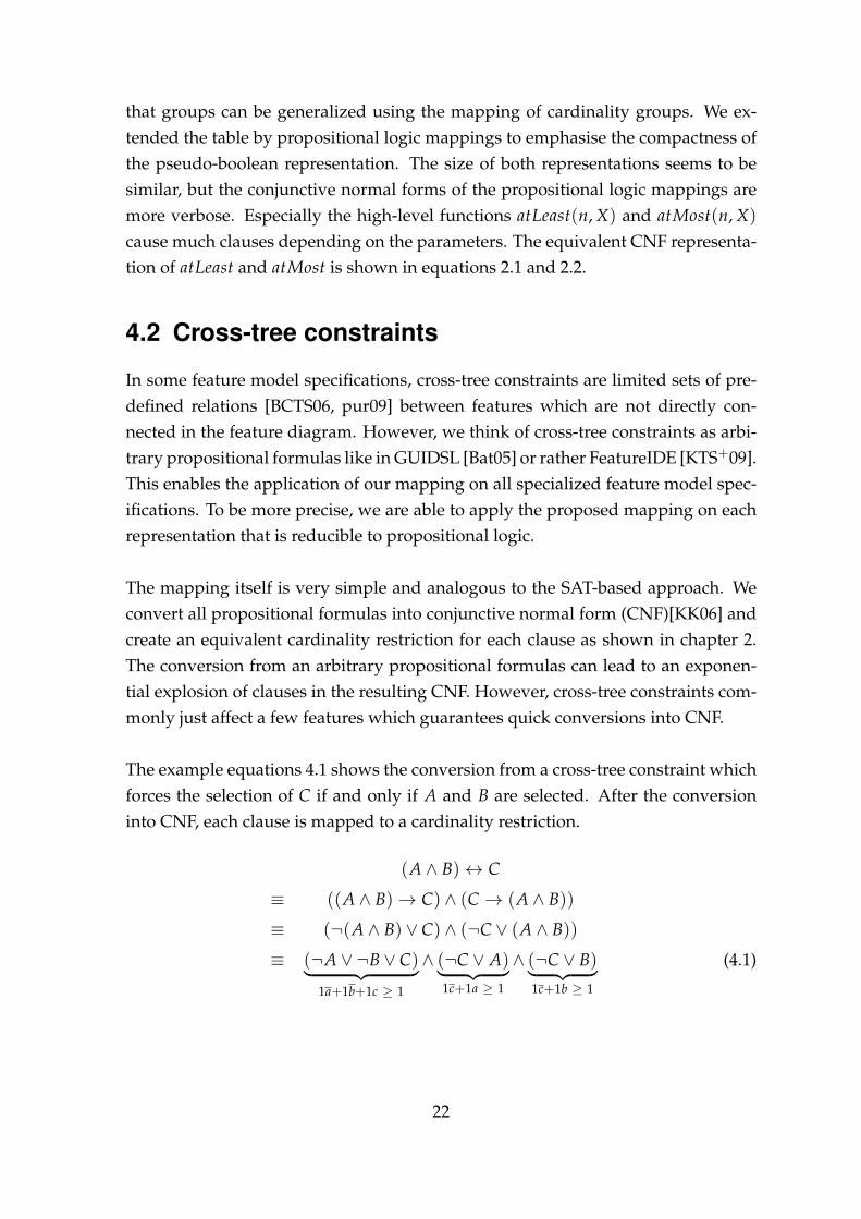
that groups can be generalized using the mapping of cardinality groups. We ex-tended the table by propositional logic mappings to emphasise the compactness ofthe pseudo-boolean representation. The size of both representations seems to besimilar, but the conjunctive normal forms of the propositional logic mappings aremore verbose. Especially the high-level functions atLeast(n, X) and atMost(n, X)

cause much clauses depending on the parameters. The equivalent CNF representa-tion of atLeast and atMost is shown in equations 2.1 and 2.2.

4.2 Cross-tree constraints

In some feature model specifications, cross-tree constraints are limited sets of pre-defined relations [BCTS06, pur09] between features which are not directly con-nected in the feature diagram. However, we think of cross-tree constraints as arbi-trary propositional formulas like in GUIDSL [Bat05] or rather FeatureIDE [KTS+09].This enables the application of our mapping on all specialized feature model spec-ifications. To be more precise, we are able to apply the proposed mapping on eachrepresentation that is reducible to propositional logic.

The mapping itself is very simple and analogous to the SAT-based approach. Weconvert all propositional formulas into conjunctive normal form (CNF)[KK06] andcreate an equivalent cardinality restriction for each clause as shown in chapter 2.The conversion from an arbitrary propositional formulas can lead to an exponen-tial explosion of clauses in the resulting CNF. However, cross-tree constraints com-monly just affect a few features which guarantees quick conversions into CNF.

The example equations 4.1 shows the conversion from a cross-tree constraint whichforces the selection of C if and only if A and B are selected. After the conversioninto CNF, each clause is mapped to a cardinality restriction.

(A ∧ B)↔ C

≡ ((A ∧ B)→ C) ∧ (C → (A ∧ B))

≡ (¬(A ∧ B) ∨ C) ∧ (¬C ∨ (A ∧ B))

≡ (¬A ∨ ¬B ∨ C)︸ ︷︷ ︸1a+1b+1c ≥ 1

∧ (¬C ∨ A)︸ ︷︷ ︸1c+1a ≥ 1

∧ (¬C ∨ B)︸ ︷︷ ︸1c+1b ≥ 1

(4.1)

22

4.3 Additional pseudo-boolean equations and

inequalities

In chapter 3, we introduced additional constraints based on pseudo-boolean re-strictions. These restrictions provide the declaration of equations and inequalitiesthat allow to refer features, attributes or even attribute sums. The mapping to thePBSAT representation is simple because of the identical form. We just have to re-place feature names by boolean variables and attribute references by their assignedvalues. The sum operator requires a replacement by all feature attributes of thereferred feature subtree according to the feature diagram. Table 4.3 shows the map-ping of features, feature attributes and sums of feature attributes from the syntaxdescribed in chapter 3. The referred features and attributes are shown in figure 4.1and 4.2. The row INTERPRETATION describes the logical consequence of the exem-plary restrictions to ease comprehension.

Figure 4.1: Subtree of a feature diagram

A.foo = 15;B.foo = 6;C.foo = 7;

Figure 4.2: Sample attribute file according to 4.1

23

RELATION GRAPHIC PROPOSITIONAL LOGIC PBSAT

root r r ≥ 1

mandatory(single)

x ↔ y x− y = 0

mandatory(in and-group)

x ↔ y1 ∧ · · · ∧ yi i · x− y1 · · · − yi = 0

optional(single)

y→ x x− y ≥ 0

optional(in and-group)

y1 ∨ · · · ∨ yi → x i · x− y1 · · · − yi ≥ 0

or(group [1,i])

x ↔ y1 ∨ · · · ∨ yi 0 ≤ i · x− y1 · · · − yi ≤ i− 1

alternative(group [1,1])

x →atLeast(1, {y1, · · · , yi}) ∧atMost(1, {y1, · · · , yi})

x− y1 · · · − yi = 0

customcardinality(group [n,m])

x →atLeast(n, {y1, · · · , yi}) ∧atMost(m, {y1, · · · , yi})

x → (n ≤ y1 + · · ·+ yi ≤ m)

⇔ i−m ≤ i · x− y1 · · · yi ≤ i− n

Table 4.2: Feature diagram mappings to PBSAT

24

TYPE SYNTAX PBSAT INTERPRETATION

feature A >= 1 a ≥ 1 A is enabledfeature attribute A.foo <= 10 a ≤ 10 A is disabled, B and C toofeature attribute sum A#foo >= 20 10a + 6b + 7c ≥ 20 A is enabled, B and/or C too

Table 4.3: Additional constraint mapping according to 4.1 and 4.2

25

5 Analysis operations

Automated reasoning is a recent topic in software product line research. In the past,various tools were used to reason on feature models. Satisfiability solver (SAT),constraint satisfaction problem (CSP) and description logic (DL) were popular tech-niques [BSRC10]. But higher level tools like Prolog [BPSP04] or data structures likebinary decision diagrams (BDD) [BSTC07] were also used. This chapter shows howPBSAT solvers can be used to reason on feature models. Therefore, several im-portant analysis operations from different authors have been adapted to reason onextended feature models in pseudo-boolean representation. The different analysisoperations will be introduced with raising complexity. The operations are sepa-rated by the stage of the engineering process they occur.

We added pseudo-code listings to describe the way the algorithms work. Therefore,some variables and functions have to be introduced. The parameter M representsa feature models which is already translated into a conjunction of pseudo-booleanrestrictions. The parameter F denotes the set of all features present in the model M.The function addAssumption() takes a model and an assumption (simple restric-tion) and returns a new model extended by the specified assumption. The functionremoveAssumptions() removes all previously added assumptions. Finally, the func-tion satis f iable() symbolizes the call to the pseudo-boolean satisfiability solver. Thecall to satis f iable() returns true if and only if there is a satisfying assignment forthe passed PBSAT instance representing the feature model.

5.1 Domain engineering

We divided this chapter in the section domain engineering and application engineering.Both terms describe a specific process in software product-line engineering. We cat-egorized the algorithms in these stages to emphasize the environment they usuallyoccur.

26

Domain engineering describes the process of collecting individual customer needsand assembling them into a feature model. In this stage, the domain engineer cre-ates and refactors the feature model. The various suggested algorithms supportdomain engineering by verifying feature models and reporting potential damages.Furthermore, changes on the model can be observed to preserve semantics. Allthese operations can run in background to inform the domain engineer if neces-sary. Automated reasoning in the domain engineering process eases developmentin software product line engineering and increases productivity.

5.1.1 Validation

Definition: A valid feature model requires that concrete products can be derivedfrom the specification. If there is no derivable product, the model is called void. Thevalidation is a basic reasoning operation since it guarantees that the model is con-sistent. Furthermore, a valid feature model is a pre-condition for deeper analysiswhich is explained later in this chapter.

Figure 5.1 illustrates the difference between valid and void feature models. Addingthe cross-tree constraint ¬A ∧ B makes the model invalid because both features areforced to be enabled cause of mandatory feature diagram relations.

Figure 5.1: A valid and a void feature model

The validation algorithm [1] is simple and straightforward. We take the featuremodel M which is represented as conjunction of pseudo-boolean restrictions callthe PBSAT solver on this representation. If the solver returns false which means“unsatisfiable”, no solution exists and hence no product. Otherwise, the model isvalid and describes real products.

27

Algorithm 1 Check validity of feature model

function ISVALID(M)return satis f iable(M)

end function

5.1.2 Feature properties

Many authors covered the properties that arise from the composition of features intheir corresponding model [BSRC10]. They found out that some features are partof every product. At least the root feature fulfils this condition all the time. Some-times, features can not be enabled during application engineering and consequentlyare never part of any derived product. In the following section, we introduce fourdifferent feature properties, give a proposal how to compute them, and examinethe strong relation between them. In figure 5.2, we introduce a feature model withdifferent feature properties. In the following section, this feature model will help tounderstand the described properties and to comprehend the proposed algorithms.

Figure 5.2: A feature model that contains features with different properties

Core features

Definition: A core feature is a component which is part in all products described bythe product line. Core features can not be disabled cause of relations and/or con-straints in the feature model. The root feature is obviously a core feature in everyfeature model.

Figure 5.3 emphasises the core feature in our example feature model. It is obvi-ous that Root and the mandatory connected A are core features. Feature B is also a

28

core feature because of the cross-tree constraint A⇒ B. The remaining features arenot contained in the set of core features.

Figure 5.3: A feature model with emphasised core features

The core feature algorithm [2] takes a feature model M and a set F of all featurespresent in the model. For each feature, we assume that it is disabled by adding anassumption to the model. If the PBSAT solver tells us that the feature is “unsatis-fiable”, we know the feature has to be part in any valid product. In other words,there is no product without the contemplated feature.

Algorithm 2 Compute set of core features

function COMPUTECOREFEATURES(M, F)Fcore ← ∅for all f ∈ F do

M← addAssumption(M, f = 0) . forces feature f to be disabledif ¬satis f iable(M) then

Fcore ← Fcore ∪ { f }end ifM← removeAssumptions(M) . remove the assumption

end forreturn Fcore

end function

Dead features

Definition: A dead feature is a component which can not be part in any product al-though it is part of the feature model. Dead features occur because of additionalconstraints which force them to be disabled.

29

Benavides et al. [BSRC10] stated dead features as anomaly. In our opinion, deadfeatures are not always problematic. They could be used to temporarily deactivatespecific functionality. Another use case could be in staged configuration[CHE05],where previous (de-)selections by another party can not be undone. This leads todisabled or rather deselected features which can be interpreted as dead features.

Figure 5.4 shows a dead feature in the example feature model. Feature D is deadbecause of the cross-tree constraint ¬(A ∧ D) and the fact that A is a core feature.

Figure 5.4: A feature model with emphasised dead features

If one selects a dead feature, the feature model becomes invalid. This characteristicexplains the correctness of our iteratively assumption-based algorithm [3]. Notice,the computation of dead features is analogical to the core feature algorithm. Theonly difference are the temporarily added assumptions.

Algorithm 3 Compute set of dead features

function COMPUTEDEADFEATURES(M, F)Fdead ← ∅for all f ∈ F do

M← addAssumption(M, f = 1) . forces feature f to be enabledif ¬satis f iable(M) then

Fdead ← Fdead ∪ { f }end ifM← removeAssumptions(M) . removes the assumption

end forreturn Fdead

end function

30

Variant features

In our opinion, there is no satisfying definition in the literature. Benavides et al.[BSRC10] defines variant features as features that do not appear in all products of asoftware product line. We propose a stronger definition of variant features. In ourmind, features can either be core, dead or variant. This definition separates dead andvariant features into two disjoint sets.

Definition: A variant feature describes a feature model component that can be en-abled or disabled. Variant features extend the variability of the feature model, be-cause their occurrence increases the number of potential products.

Figure 5.5 highlights all variant feature in the example feature diagram. The fea-tures C and E are variant because they are neither core nor dead features.

Figure 5.5: A feature model with emphasised variant features

The variant feature algorithm [4] takes the feature model M and a set of all featuresF. After computing core and dead features, the variant features can easily be deter-mined. Variant features are those features that are neither core nor dead.

Algorithm 4 Compute set of variant features

function COMPUTEVARIANTFEATURES(M, F)Fcore ← computeCoreFeatures(M, F)Fdead ← computeDeadFeatures(M, F)Fvariant ← F \ (Fcore ∪ Fdead)return Fvariant

end function

31

Notice that the previously introduced properties are strongly related to each other.The computation can be combined in just one loop calling the satisfiability solverat all for O(2n) times where n denotes the number of features. Additionally, thefollowing equations hold:

F = Fcore ∪ Fdead ∪ Fvariant (5.1)

|F| = |Fcore|+ |Fdead|+ |Fvariant| (5.2)

False-optional features

Definition: A false-optional feature is a component that seems to be optional althoughit is part of all valid products. False-optional features are obviously a subset of corefeatures. Making false-optional features visible helps to restructure feature modelswhile semantics are preserved.

Figure 5.6 emphasises the only false-optional feature in the example model. Fea-ture B is core but at the same time not mandatory connected to the parent featureRoot which makes it false-optional.

Figure 5.6: A feature model with emphasised false optional features

At first, the false-optional algorithm [5] determines all core features. After that, thecore features will be checked whether they are optional or not. This is done by theisOptional() function. The result are all core features in a optional relation whichfits exactly the above definition.

32

Algorithm 5 Compute set of false-optional features

function COMPUTEFALSEOPTIONALFEATURES(M, F)Fcore ← computeCoreFeatures(M, F)Ff alseOpt = ∅for all f ∈ Fcore do

if isOptional( f ) thenFf alseOpt ← Ff alseOpt ∪ { f }

end ifend forreturn Ff alseOpt

end function

5.1.3 Simplification

In almost all feature models, there are groups of features which can be handled asa single feature. In other words, if you select one feature of such a group, the se-lection will be propagated to all remaining features of the group. These groups arebetter known as atomic sets[ZZM04]. Each atomic set can be handled like a singlefeature in the mapping procedure. This enables simplification through replacementof features or rather variables. The consequence are fewer features and a more com-pact representation. Furthermore, atomic sets make the real variability of a featuremodel visible.

Figure 5.7 illustrates how a feature model can be simplified by replacement ofstrongly connected features. Notice that the cross-tree constraint B ⇔ C is con-sidered in the simplification.

Figure 5.7: Simplification of a feature model with atomic sets

33

In the past, atomic sets were generated by traversal through the feature diagram[Seg08].The algorithm grouped features which have a mandatory relation to each other. Allthose groups were merged which caused a simplification that decreased the num-ber of variables and clauses[ZZM04]. Cross-tree constraints and other informationattached to the feature model were skipped. To respect all the given informationencoded in the feature model, we extended the traversal-based algorithm. We builta divide and conquer algorithm that is based on assumptions like the previously pre-sented algorithms. This extension allows us to find all atomic sets in the featuremodel.

The simplification algorithm [6] takes a feature model M and a set of features F.At the initial call, F contains all features. In subsequent (recursive) calls, the setF contains just subsets of features which are potential atomic sets. The basic ideaof the proposed algorithm is, to split F into two disjoint sets of features until wefind an atomic set. As soon as we find an atomic set, we can merge features orrather simplify the feature model. An atomic set is found if |F| = 1 (trivial case) oreach selection of a feature in F forces all remaining features to be enabled (by proof).

Proof: Let M be the PBSAT representation of the feature model. Let F be a setof features with |F| > 1. Let f ∈ F and G = F \ { f }. The set F is atomic if andonly if the selection of each feature f ∈ F forces all remaining features g ∈ G tobe enabled. Assume f is enabled ( f = 1) and g is disabled (g = 0). If the PBSATsolver determines that this expression is "unsatisfiable", we know that the followingcondition holds for feature model M.

¬satis f iable(M ∧ f = 1∧ g = 0) ⇒ M ∧ f = 1→ g = 1 (5.3)

If we do this assummption-based check for each f ∈ F and each g ∈ G and showunsatisfiability of each combination, we know that F is an atomic set.

∀ f ∈ F : ∀g ∈ G : ¬satis f iable(M ∧ f = 1∧ g = 0)

⇒ ∀ f ∈ F : ∀g ∈ G : M ∧ f = 1→ g = 1

⇒ F is atomic set

(5.4)

For most calls to this procedure, F will not be an atomic set. In this case, we splitthe set of features as soon as possible. If the inner loop detects that the selection

34

propagates not to all g ∈ G, we split F into those features that were affected by thepropagation including f and those which were not affected.

It is not required to run the traversal-based algorithm before applying our pro-posed one. The result will be the same in both cases. But we assume that thepre-processing by the traversal-based algorithm will accelerate the total runtime.

Algorithm 6 Compute the atomic sets

procedure COMPUTEATOMICSETS(M, F)if |F| = 1 then

simpli f y(M, F)return

end iffor all f ∈ F do

G ← F \ { f }H ← ∅for all g ∈ G do

M← addAssumptions(M, f = 1∧ g = 0) . enables f ; disables gif ¬satis f iable(M) then

H ← H ∪ {g}end ifM← removeAssumptions(M) . remove assumptions

end forif G 6= H then

computeAtomicSets(M, H ∪ { f })computeAtomicSets(M, F \ (H ∪ { f }))return

end ifend forsimpli f y(M, F)return

end procedure

Performance adaptations

We already mentioned that the proposed algorithm is based on the divide and con-quer design paradigm which provides parallel execution. Each (sub-)call of thecomputeAtomicSets() procedure can be processed independently. To accomplishconcurrency, the simpli f y() function has to prevent race conditions. It can either

35

apply the simplifications after the computation of the atomic sets or it needs syn-chronization to simplify the feature model during parallel execution. Both variantswill differ in implementation effort as well as performance. Given this extension,we are able to accelerate the runtime especially on large-scale feature models.

5.1.4 Edits

Definition: A feature model edit describes any modification on a feature model. Mod-ifications occur during the development process of feature models. Adding, delet-ing or changing features and/or constraints are edits. Each edit affects the under-lying representation of the feature model that causes semantic changes. Analysingthese semantic changes allows to specify feature model edits.

Classifications of edits help to observe changes on the feature model. This allowsto assist the domain engineer during feature modeling. Changes in the representedproducts will be reported and help to preserve semantics. Especially refactoringsbenefit from the categorization of feature model edits.

Figure 5.8 illustrates a modification on the feature model that is caused by adding anew feature C. The analysis will infer that new products were generated but nonewere eliminated. This observation is required to state the modification as general-ization.

Figure 5.8: A feature model edit that is classified as generalization

Feature model edits are specified by analysis of the represented products. The anal-ysis basically compares the feature model before and after the edit. It determineswhether new variants have been generated and if variants have been eliminated.The edit types are either refactoring, generalization, specialization or arbitrary edit. Weintroduce L( f ) as the set of all products represented by feature model f . Figure 5.9

36

shows the four different edit types and their respective requirement which is ex-pressed as subset relation of L( f ). Notice that g represents the feature model afterthe edit.

L(g) ⊆ L( f ) L(g) * L( f )(no products added) (products added)

L( f ) ⊆ L(g)(no products deleted)

L( f ) = L(g) L( f ) ⊂ L(g)(Refactoring) (Generalization)

L( f ) * L(g)(products deleted)

L(g) ⊂ L( f )(Specialization) (Arbitrary Edit)

Figure 5.9: Types of edits based on set inclusions or rather logical implications

Thüm et al. [TBK09] discovered a way to reason on feature model edits using atraditional SAT solver. This approach is based on the relation between L( f ) andthe propositional logic representation. We already mentioned in chapter 2 that thenumber of products and the number of satisfying assignments of the propositionallogic representation is equal. Therefore, let P( f ) be the propositional logic repre-sentation of f , which is primarily in CNF. Let v be a combination of features. If andonly if v ∈ L( f ), then v is a valid product and consequently satisfies P( f ) by as-signing all contained features of v to true. The connection between L and P allowsto verify subset relation by logical implications as shown in 5.5.

L( f ) ⊆ L(g) ≡ P( f )⇒ P(g) (5.5)

Thüm noticed that the conversion of P( f ) → P(g) to CNF took much more timethan the call to the SAT solver. The reason was the exponential explosion of clausescaused by ¬P( f ). An improved technique called simplified reasoning was intro-

37

duced. It provides a sophisticated way using multiple SAT solver calls and avoid-ing the time-consuming CNF conversion. It is based on the fact that P( f ) and P(g)are very similar CNFs. Equation 5.6 declares c as the identical clauses whereas p f

and pg are the distinct clauses.

P( f ) = p f ∧ c

P(g) = pg ∧ c(5.6)

The simplified reasoning [TBK09] is based on the equivalence illustrated in 5.7. Theresulting propositional formula consists of a disjunction of Ii for i ∈ {1, · · · , n}.The Ii represents the expression P( f ) ∧ ¬Ri whereas each Ri for i ∈ {1, · · · , n} is aclause that arises by splitting the CNF pg. The simplified reasoning checks satisfia-bility of each Ii independently. Therefore, we have up to n calls to the SAT solver.If one of the calls determines satisfiability, we know that P( f ) ; P(g) holds. Oth-erwise, P( f )⇒ P(g) is valid.

P( f ) ; P(g)

≡ P( f ) ∧ ¬pg

≡ (P( f ) ∧ ¬R1)︸ ︷︷ ︸=I1

∨ · · · ∨ (P( f ) ∧ ¬Rn)︸ ︷︷ ︸=In

(5.7)

Determining edit types using the PBSAT representation is similar to the presentedapproach. We just have to deal with linear equations and inequalities instead ofCNF clauses. Therefore, we have to customize the presented approach slightly. Thecomplete equivalence proof from 5.7 can be applied by thinking of equations andinequalities instead of clauses. The only adaption is the negation of the Ri’s, whichneeds a little bit more work when treating equations and inequalities instead ofclauses. Negating inequalities is trivial because of the discrete space. The equationsin 5.8 visualize the procedure. Notice that we adjust the degree by +1 or rather −1to preserve the pseudo-boolean representation.

¬(n

∑i=1

aixi ≥ d) ⇔n

∑i=1

aixi ≤ d− 1

¬(n

∑i=1

aixi ≤ d) ⇔n

∑i=1

aixi ≥ d + 1(5.8)

38

The negation of equations does not necessarily need more effort. The easiest way isthe separation in two inequalities I′i and I′′i which also requires two PBSAT solvercalls instead of one. A smarter approach is the transformation from a disjunction ofinequalities to a conjunction of inequalities. This allows the analysis in just one callof the PBSAT solver.

¬(n

∑i=1

aixi = d)

⇔n

∑i=1

aixi 6= d

⇔n

∑i=1

aixi > d ∨n

∑i=1

aixi < d

⇔n

∑i=1

aixi ≥ d + 1 ∨n

∑i=1

aixi ≤ d− 1

⇔n

∑i=1

aixi ≥ d + 1 ∨ −n

∑i=1

aixi ≥ −d + 1

⇔n

∑i=1

aixi ≥ d + 1︸ ︷︷ ︸=d′

∨n

∑i=1

aixi ≥ −d + 1 +n

∑i=1

ai︸ ︷︷ ︸=d′′

(5.9)

The arithmetic conversion in 5.9 is required to transform the logical operator. Theconversion is based on the discrete space and equation 2.4. Equivalence 5.10 showsthe transformation of the disjunction into a conjunction. The applied technique issimilar to the reduction from the NP-complete problems “SAT” to “3SAT” [GJ79].We have to introduce an auxiliary variable y to ensures satisfiability of both inequal-ities. If one of the inequalities is satisfied, the other becomes automatically satisfiedby the right choice of y.

satis f iable

(n

∑i=1

aixi ≥ d′ ∨n

∑i=1

aixi ≥ d′′)

⇔ satis f iable

(d′y +

n

∑i=1

aixi ≥ d′ ∧ d′′y +n

∑i=1

aixi ≥ d′′) (5.10)

The adaption to PBSAT has several advantages according to the reasoning perfor-mance. We already mentioned the compactness of the PBSAT representation. PB-SAT instances are usually shorter than equivalent CNF instances. Therefore, fewerRi’s occur during simplified reasoning which decreases the number of calls to the

39

solver. We additionally benefit from the existence of equations in the Ri’s becausewe do not need to split them in two separate inequalities. The presented negationuses an auxiliary variable to avoid unnecessary computation.

Thüm proposed two required extensions to handle addition and deletion of fea-tures as well as abstract features[TKES11]. Without those extensions, the results ofthe edit type reasoning would be wrong in some cases. The extension for addedand removed features determines if new features have been added or existing fea-tures have been deleted. In this is the case, those features have to be disabled in themodel they do not occur. This can be done by adding an assumption. We alreadyhandled assumptions in the previous algorithms. Disabling an arbitrary feature Acan obviously be achieved by adding the inequality a ≤ 0 to the PBSAT instance.The second extension for abstract features eliminates variables which represent ab-stract features. This is necessary because abstract features are code-less and thereforedid not extend variability of the product line. We eliminate these variables by re-placements known from linear equation systems. For each variable representing anabstract feature, we look for an equation to replace all occurrences of this variablein the remaining pseudo-boolean restrictions.

5.2 Application engineering

Application engineering describes the process of selecting and deselecting features toderive products. The configuration of products needs a feature model that definesthe product line. This enables tool support to handle propagations of feature se-lections and provides explanations. Additionally, automated tool support preventsfrom building invalid products. The presented algorithm minimizes configurationeffort and speeds up application engineering. Notice that we will use the term fea-ture selection or rather selection to describe selections as well as feature deselections.The former describes addition of features where the latter means the exclusion offeatures.

5.2.1 Propagation of selections

Definition: Propagations are implicit feature selections that arise by manually select-ing features during product derivation. The use of propagations can help to save

40

time because most of the selections can be done automatically according to the fea-ture diagram and the cross-tree constraints. Furthermore, automatic selections pro-hibit to select contradictory or rather invalid products.

Propagations can be determined in different ways. One possible way is to encodeselections in the feature model. This can be achieved by adding assumptions toforcedly enable or disable features. Afterwards, we run the core and dead featurealgorithms to determine selections and deselections, respectively. The disadvan-tage of this approach are numerous calls to the SAT solver.

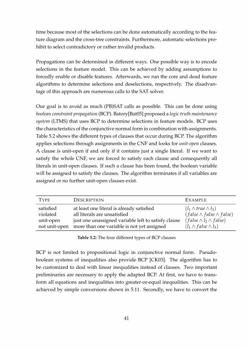
Our goal is to avoid as much (PB)SAT calls as possible. This can be done usingboolean constraint propagation (BCP). Batory[Bat05] proposed a logic truth maintenancesystem (LTMS) that uses BCP to determine selections in feature models. BCP usesthe characteristics of the conjunctive normal form in combination with assignments.Table 5.2 shows the different types of clauses that occur during BCP. The algorithmapplies selections through assignments in the CNF and looks for unit-open clauses.A clause is unit-open if and only if it contains just a single literal. If we want tosatisfy the whole CNF, we are forced to satisfy each clause and consequently allliterals in unit-open clauses. If such a clause has been found, the boolean variablewill be assigned to satisfy the clauses. The algorithm terminates if all variables areassigned or no further unit-open clauses exist.

TYPE DESCRIPTION EXAMPLE

satisfied at least one literal is already satisfied (l1 ∧ true ∧ l3)violated all literals are unsatisfied ( f alse ∧ f alse ∧ f alse)unit-open just one unassigned variable left to satisfy clause ( f alse ∧ l2 ∧ f alse)not unit-open more than one variable is not yet assigned (l1 ∧ f alse ∧ l3)

Table 5.2: The four different types of BCP clauses

BCP is not limited to propositional logic in conjunctive normal form. Pseudo-boolean systems of inequalities also provide BCP [CK03]. The algorithm has tobe customized to deal with linear inequalities instead of clauses. Two importantpreliminaries are necessary to apply the adapted BCP. At first, we have to trans-form all equations and inequalities into greater-or-equal inequalities. This can beachieved by simple conversions shown in 5.11. Secondly, we have to convert the

41

left-hand side of the inequality to get only positive coefficients. The procedure totransform all coefficients positive is explained in chapter 2.

n

∑i=1

aixi ≤ d ⇔ −n

∑i=1

aixi ≥ −d

n

∑i=1

aixi = d ⇔n

∑i=1

aixi ≤ d ∧n

∑i=1

aixi ≥ d(5.11)

The basic functioning of the pseudo-boolean BCP is identical to the propositionallogic version. Just the definitions of satisfied, violated, unit-open and not unit-openare different. Table 5.4 shows the definitions. An inequality is unit-open if and onlyif the variable with the biggest coefficient has to be satisfied to avoid violation. Aviolation occurs if the sum of all coefficients ∑n

i=1 ai is smaller than the degree d. Inother words, even if all variables are satisfied, the inequality can not be valid. Eachunit-open inequality produces new assignments which allow further propagations.The adapted BCP also stops if all variables were assigned or no unit-open inequal-ities exist anymore.

TYPE DEFINITION

satisfied d ≥ 0

violatedn∑

i=1< d

unit-openn∑

i=1ai ≥ d >

n∑

i=1ai − ak

not unit-open inequality is neither satisfied, violated or unit-open

Table 5.4: The four different types of BCP inequalities

Figure 5.10 shows a sample feature model where feature B was selected. This startspropagation which leads to the selection of feature D because of the constraintB ⇒ D. Moreover, feature E will be deselected because of the alternative grouprelation. Figure 5.11 illustrates the propagations of the pseudo-boolean BCP in a di-rected graph. The nodes represent assignments. The directed edges are annotatedwith the unit-open inequality that leads to new assignments. Notice that featureRoot and C are core features and hence already assigned. Otherwise, the presentedinequality −c + d + e = 0 would not be unit-open.

42

Figure 5.10: A user selection leads to a propagation

b=1

d=1

-b +d >= 0

e=0

-c +d +e = 0

Figure 5.11: The propagation of 5.10 represented as graph

Both BCP algorithms are not complete which means that further propagations mayexist. Therefore, all remaining features, which assignments have not been inferred,have to be checked by the (PB)SAT solver. We can use the core and dead featurealgorithms as previously described.

43

6 Evaluation

The evaluation shall underline the applicability of the proposed analysis operationsfor the development of software product lines. We are interested in fast algorithmsthat allow quick responses. Minimizing the required runtime enables better userinteraction in graphical tools like FeatureIDE and pure::variants. Therefore, wemainly focussed on the required computation time for selected algorithms. But wealso examined the simplification potential of the contemplated feature models. Atlast, we tried to verify our assumption regarding the pre-processing to speed-upsimplification. The evaluations revealed some unexpected results which may havean influence on further implementations.

We run the evaluation on an Intel Core 2 Duo CPU with a clock rate of 2 giga-hertz. The installed operating system was a Linux system with kernel 2.6.35-30 (64bit). The algorithms were executed on an OpenJDK1 virtual machine for Java 6. Weused the PBSAT solver of the SAT4J project2 as reasoning engine. We measured therequired time of the different analysis operations to check scalability. All contem-plated algorithms were executed 100 times before we determined the arithmeticmean. We used the JAVA-method System.nanotime() to determine the current timein nanoseconds. The stated times are all converted to milliseconds to ease compar-ison.

We used 11 real-world feature models of different software product lines from theFeatureIDE repository. Most of the feature models contain between 20 and 30 fea-tures. But we still have three larger models with more than 70 features whereaseach of them has at least 20 additional constraints.

1 http://openjdk.java.net/2 http://sat4j.org/

44

6.1 Runtime behaviour

Table 6.1 shows the analysed feature models with feature and constraint count aswell as required time for different analysis operations. The column VALIDATION

specifies the required time to determine whether the feature model is valid or void.It seems that the required processing time of the validation scales very well forfeature models with less than a few hundred features. The PROPERTIES-columndefines the required time to obtain the four different feature properties. We al-ready mentioned in chapter 5 that the computation of dead, core, variant and false-optional features can be done in a compound algorithm. Therefore, we needO(2n)calls to the PBSAT solver where n denotes the number of features. We see that therequired time increases very fast depending on the number of features. The last col-umn PROPAGATION shows the required time to propagate a selection in the featuremodel. We evaluated the time by iteration over all features. We selected and des-elected each features 100 times and determined the mean time until BCP stopped.We observe increasing time for larger models. But the algorithm scales very welleven for the largest feature model.

MODEL #FEAT. #CONSTR. VALIDATION PROPERTIES PROPAGATION(in ms) (in ms) (in ms)

FameDB2 21 1 0.543 6.089 0.825FameDB 22 0 0.305 6.910 0.620APL 23 2 0.194 3.530 0.838SafeBali 24 0 0.204 3.818 0.688Chat 25 1 0.230 4.561 0.663APL-Model 28 8 0.224 4.635 0.767TightVNC 28 3 0.207 4.623 0.636GPL 38 15 0.605 8.359 2.217BerkeleyDB 76 20 0.482 17.556 2.263Violet 101 27 0.503 24.557 4.244E-Shop 326 21 0.972 140.199 7.304

Table 6.1: Mean runtime of validation, property computation and propagation

6.2 Simplification potential

We extended the algorithm of atomic sets to guarantee maximum possible simpli-fication of the feature model. Atomic sets allow to consider groups of features as

45

a single feature. Hence, atomic sets reduce the number of required variables andallow simplification of the underlying representation. The simplification eliminatesredundant or rather satisfied entities of the representation. In our context, these en-tities are pseudo-boolean restrictions. Table 6.2 shows the number of features andrestrictions for each feature model. Additionally, the number of atomic sets and re-strictions after the computation are listed. We observed that all feature models hadsimplification potential. The potential varies between 2% in the Violet model and58% in the SafeBali model. Even the largest feature model had a high simplificationrate of 35%.

BEFORE COMPUTATION AFTER COMPUTATIONMODEL #FEAT. #RESTR. #AS’S #RESTR.

FameDB2 21 18 15 -29% 12 -33%FameDB 22 16 15 -32% 9 -44%APL 23 24 15 -35% 16 -33%SafeBali 24 21 10 -58% 7 -67%Chat 25 22 20 -20% 17 -23%APL-Model 28 36 24 -14% 32 -11%TightVNC 28 16 23 -18% 11 -31%GPL 38 46 26 -32% 34 -26%BerkeleyDB 76 109 54 -29% 80 -27%Violet 101 143 99 -2% 141 -1%E-Shop 326 294 212 -35% 179 -39%

Table 6.2: Results of the simplification (atomic set) computation

6.3 Pre-processing impact

In chapter 5, we assumed that the traditional tree-traversal algorithm for atomicsets is an efficient pre-processing for our extended algorithm. It turned out that thisassumption seems to be wrong. The evaluation revealed that the pre-processingdoes not accelerate the required runtime. Furthermore, we noticed that the numberof calls to the PBSAT solver does not correlate with the runtime. In some models,the computation of atomic sets was faster with pre-processing. In other models, theruntime without pre-processing had a better performance. Table 6.3 contains theresults of our evaluation. We measured the time as well as the number of necesarry

46

call to the satisfiability solver. In most of the cases, the performance without pre-processing was better although more PBSAT calls were needed. The best exampleis the SafeBali model that needed more than 3 times PBSAT calls with disabled pre-processing. But the required time for the whole computation was still faster thanthe version with enabled pre-processing.

+PRE-PROCESSING -PRE-PROCESSINGMODEL RUNTIME SAT CALLS RUNTIME SAT CALLS

FameDB2 32.250 105 22.250 -31% 138 +24%FameDB 22.218 105 20.514 -8% 151 +30%APL 21.050 102 19.708 -6% 139 +36%SafeBali 12.950 45 11.966 -7% 164 +264%Chat 33.667 180 37.925 +13% 190 +6%APL-Model 50.659 254 31.607 -38% 203 -20%TightVNC 48.384 252 33.137 -32% 208 -21%GPL 45.906 237 56.756 +24% 385 +62%BerkeleyDB 200.078 1169 201.313 +1% 1648 +41%Violet 773.947 3186 639.629 -17% 2592 -23%E-Shop 3817.053 18672 3605.623 -6% 20238 +8%

Table 6.3: Mean runtime of the simplification (atomic set) algorithm

47

7 Conclusion

In this thesis, we proved that linear pseudo-boolean instances are able to repre-sent feature models. We developed a mapping that allows independent transla-tion of feature model components to PBSAT instances. Furthermore, we discoveredthat PBSAT instances allow handling and reasoning of integer attributes in featuresmodels. We proposed a special attribute file to assign values to feature attributes.Moreover, we also introduced another file to define additional constraints whichcan refer attributes.

Satisfiability solvers that work on the PBSAT representation allow similar reason-ing as traditional SAT solvers. Therefore, we took different known feature modelanalysis operations and adapted them to work with a PBSAT solver. Simple algo-rithms needed almost no adaption. More sophisticated algorithms required deeperknowledge of the PBSAT representation and possible conversions. Some adaptedalgorithms enabled reasoning with fewer calls to the PBSAT solver. But fewer callsnot necessarily indicated faster execution. We could not find analysis operationsthat are not feasible with the PBSAT representation.

In our evaluation, we saw that some algorithms scale very well. Especially thevalidation and the propagation algorithm. Other algorithms, which needed manyPBSAT solver calls, slowed down if the number of features and additional con-straints increased too much. The evaluation revealed that all feature models havesimplification potential. This is very useful for refactoring and improving perfor-mance of other analysis operations. The evaluation also showed that the numberof SAT calls does not correlate with the required time to look for satisfying assign-ments. We also verified that the pre-processing by the tree-traversal algorithm didnot accelerate our proposed algorithm.

48

7.1 Contributions

The main contribution of the thesis is the usability of PBSAT problems to reason onfeature models. In chapter 4, we examined how (extended) feature models can bemapped to PBSAT instances in the most compact representation.

During the adaption of the algorithms, we observed potential for further improve-ment and therefore extended existing analysis operations. We extended the simpli-fication algorithm to find all existing atomic sets which ensures maximum simplifi-cation. The proposed algorithm supports the divide and conquer design paradigmthat enables parallel execution. We also found out that reasoning of feature modeledits using the PBSAT representation needs fewer calls to the solver. Further callscan be saved if our proposed conversion for equations will be used. In addition, weproposed the distinction between tree-based atomic sets and real atomic sets since thewidely known tree-traversal algorithm does not detect all atomic sets.

We also proposed a new definition of the term variant feature to have a clear dis-tinction between feature properties. In our point of view, features are either core,dead and variant.

We found out the PBSAT instances are well suited to represent feature models.The compactness and the expressiveness are the major benefits of this represen-tation. Additionally, it allows us to define cardinality-based feature models easilyand supports feature attributes.

7.2 Further work

During this thesis, we found several interesting issues we want to address in nearfuture. This section gives a brief overview about the related topics we want to dealwith.

Inspired by the logic truth maintenance system (LTMS) proposed by Batory[Bat05],we want to check feasibility of explanations using a PBSAT solver. Explanationsdescribe automatic propagation in a human-readable way. This helps users to com-prehend automatic selection during product derivation.

49

PBSAT solvers usually provide an objective function that allow to find optimal so-lutions. An optimal solution is a satisfying assignment which maximizes (or min-imizes) the value of the objective function. We want to use this target function toderive optimal products based on different objectives.

The evaluation in this thesis used 11 different real-world feature models from soft-ware projects. In future, we want to enlarge our repository of feature models to getmore representative evaluation results. Therefore, we will gather variability mod-els from different business sectors.

We are also interested in a comprehensive performance comparison of SAT andPBSAT. Therefore, we have to implement missing analysis operation based on aSAT reasoning engine.

50

Bibliography

[Bat05] Don S. Batory. Feature models, grammars, and propositional formu-las. In Proc. Int. Software Product Line Conference (SPLC), pages 7–20.Springer, 2005.

[BCTS06] David Benavides, Antonio Ruiz Cortés, Pablo Trinidad, and Sergio Se-gura. A survey on the automated analyses of feature models. In Proc.Jornadas de Ingeniería del Software y Bases de Datos (JISBD), pages 129–134, 2006.

[BHP08] Timo Berthold, Stefan Heinz, and Marc E. Pfetsch. Solving pseudo-boolean problems with scip. Technical Report 08-12, ZIB, Takustr.7,14195 Berlin, 2008.

[BPSP04] Danilo Beuche, Holger Papajewski, and Wolfgang Schröder-Preikschat.Variability management with feature models. Jour. Science of ComputerProgramming (SCP), 53(3):333–352, 2004.

[BSRC10] David Benavides, Sergio Segura, and Antonio Ruiz-Cortés. Automatedanalysis of feature models 20 years later: A literature review. Informa-tion Systems, 35(6):615–636, 2010.

[BSTC07] David Benavides, Sergio Segura, Pablo Trinidad, and Antonio RuizCortés. Fama: Tooling a framework for the automated analysis offeature models. In Proc. Int. Workshop Variability Modelling of Software-intensive Systems (VaMoS), pages 129–134. The Irish Software Engineer-ing Research Centre, 2007.

[BTRC05a] David Benavides, Pablo Trinidad, and Antonio Ruiz-Cortés. Auto-mated Reasoning on Feature Models. In Proc. Int. Conf. Advanced In-formation Systems Engineering (CAiSE), pages 381–390. Springer, 2005.

51

[BTRC05b] David Benavides, Pablo Trinidad, and Antonio Ruiz-Cortés. UsingConstraint Programming to Reason on Feature Models. In Proc. Int.Conf. Software Engineering & Knowledge Engineering (SEKE), pages 677–682. Knowledge Systems Institute, 2005.

[CHE05] Krzysztof Czarnecki, Simon Helsen, and Ulrich Eisenecker. Staged con-figuration through specialization and multilevel configuration of fea-ture models. Software Process: Improvement and Practice, 10(2):143–169,2005.

[CK03] Donald Chai and Andreas Kuehlmann. A fast pseudo-boolean con-straint solver. In Proc. Design Automation Conference (DAC), pages 830–835. ACM Press, 2003.

[CW07] Krzysztof Czarnecki and Andrzej Wasowski. Feature diagrams andlogics: There and back again. In Proc. Int. Software Product Line Confer-ence (SPLC), pages 23–34. IEEE Computer Society, 2007.

[GJ79] Michael R. Garey and David S. Johnson. Computers and Intractability: AGuide to the Theory of NP-Completeness. W. H. Freeman, 1979.

[KK06] Martin Kreuzer and Stefan Kühling. Logik für Informatiker (in German).Pearson, 2006.

[KTS+09] Christian Kästner, Thomas Thüm, Gunter Saake, Janet Feigenspan,Thomas Leich, Fabian Wielgorz, and Sven Apel. Featureide: A toolframework for feature-oriented software development. In Proc. Int.Conf. Software Engineering (ICSE). IEEE Computer Society, 2009.

[pur09] pure-systems GmbH. pure::variants User’s Guide: Version3.0 for pure::variants 3.0, 2009. Source: http://www.

pure-systems.com/fileadmin/downloads/pure-variants/

doc/pv-user-manual.pdf.

[Seg08] Sergio Segura. Automated Analysis of Feature Models Using AtomicSets. In Proc. Int. Software Product Line Conference (SPLC), pages 201–207.Lero Int. Science Centre, 2008.

52

[TBK09] Thomas Thüm, Don S. Batory, and Christian Kästner. Reasoning aboutedits to feature models. In Proc. Int. Conf. Software Engineering (ICSE).IEEE Computer Society, 2009.

[TKES11] Thomas Thüm, Christian Kästner, Sebastian Erdweg, and Norbert Sieg-mund. Abstract Features in Feature Modeling. In Proc. Int. SoftwareProduct Line Conference (SPLC), pages 191 –200, 2011.

[WLS+07] Hai H. Wang, Yuan Fang Li, Jing Sun, Hongyu Zhang, and Jeff Pan.Verifying feature models using owl. Jour. Web Semantics, 5(2):117–129,2007.

[ZZM04] Wei Zhang, Haiyan Zhao, and Hong Mei. A propositional logic-basedmethod for verification of feature models. In Formal Methods and Soft-ware Engineering, pages 115–130. Springer, 2004.

53

Statutory declaration

Hereby I declare that I have written this bachelor thesis by my own. Furthermore,I confirm that no other sources have been used than those specified in the bachelorthesis itself. This thesis, in same or similar form, has not been available to any auditauthority yet.

Passau, October 28, 2011

Sebastian Henneberg